1

Technical paper submitted for presentation at International Conference on CAD and CG, Hong Kong, 7-10 December 2005

Voxel-based Representation, Display and Thickness Analysis of Intricate Shapes

Sandeep Patil, M.Tech. Student

B. Ravi, Associate Professor Indian Institute of Technology Powai, Mumbai 400076, India

E-mail: bravi@me.iitb.ac.in Abstract This paper presents a novel voxel-based representation scheme coupled with voxelisation, display and geometric algorithms for the purpose of thickness analysis of very complex free form shapes. The binary voxel model is stored as a stack of voxel layers represented as bit-arrays. Polygonal solid models obtained from a CAD system or 3D scanning are converted into voxel format with a maximum resolution of 1000 (overall volume of 1 billion voxels) in less than 2 minutes. Near real-time visualization of the voxel model is achieved by direct point rendering using a look-up table based on a finite set of neighbour voxel configurations. This gives better images than simple cube face display that has blocky appearance. Geometric computation functions have been developed to perform thickness analysis in terms of cross-sectional visualisation, progressive skin removal and radiography with minimum, maximum and total thickness along an orthographic direction. Testing of the algorithms for intricate shapes like a Ganesha idol, pelvic bone and cylinder block gave satisfactory results. The voxel based framework can be coupled to a standard CAD system, providing additional capabilities to product designers. Keywords: Voxel, Solid modeling, Geometric reasoning, Computer-Aided Design. 1. Introduction Volumetric or voxel-based modeling is based on an approximate representation of a 3D object in terms of a set of tiny volume elements. Its growing importance is driven by its ability to capture extremely complex free form shapes and those with anisotropic or heterogeneous internal properties, thus better mimicking real world objects. They are suited to natural acquisition, such as CT/MRI scanning, and easily allow Boolean modeling operations. The major limitation is the requirement of large memory (to minimize discretisation error) and processing time (for display and analysis). The most general representation of a voxel model is the exhaustive enumeration of the occupancy of voxels lying on a uniform 3D grid. For each cell, either a binary value is stored indicating the presence or absence of material, or a numeric value is stored representing a physical quantity such as density. A 3D array (also called volume buffer, cubic frame buffer, or 3D raster) is typically used to store these values in a uniform grid aligned with the coordinate axes [Kaufman, 1993]. A binary voxel model is usually obtained by ‘voxelisation’, which involves conversion from a CAD model available in B-Rep format. Our work was motivated by the need to explore voxel-based modeling to perform geometric reasoning (such as thickness analysis) on complex freeform shapes (such as sculptures and medical models). The goal was to obtain less than 1% error on typical sized parts (up to 1000 mm), which required 1000 voxels per axis, or a maximum of 1 billion voxels. The major routines: voxellisation, display and analysis, were aimed to be completed within 1-2 minutes each on a standard Pentium computer running Windows operating system.

2

The next section reviews previous work in voxel model representation, voxellisation, display, and applications. This is followed by our scheme for the above tasks, implementation, and results on three real-life complex shapes. 2. Previous work 2.1 Voxel model representation Ideally, the voxel model representation scheme must allow efficient storage, interactive display, desired manipulations, data availability and representation conversions [Jense, 1989]. There are many methods proposed for voxelization of polygon models [Nooruddin, 2003] and CSG models [Fang, 2000], based on different representation schemes for voxel models. The two most important schemes are array and octree implementation. Octree methods, in which each node has eight children, achieve data compression by storing voxel information in a hierarchical tree structure, which is built in a top-down fashion by recursively subdividing inhomogeneous regions of the volume into eight sub-regions until each terminal node of the tree corresponds to a region of the volume in which all voxels share the same value [Prakash, 1990]. Actual implementation of octree uses pointers for representing connections between parent and sibling nodes at every stage of partitioning. In contrast, array implementation is much more simple and straight forward. Also, for realistic representation of highly complex shapes, the octree grows closer to its full size, and the array implementation may even be more efficient than octree in terms of storage. This is because for every node in the octree, we must store pointers to its parent and eight siblings. This is unnecessary if their location is implicit, as in an array index of the nodes. There are many possible variations in array representation of voxel models. Many commercial software packages have their own custom formats. The simplest array implementation would be for a binary voxel model wherein a single bit can be used to represent the state of each voxel. For gray scale voxel model, depending upon the range of the variable for each voxel, an array of appropriate data type is used. 2.2 Voxelisation Voxelisation (also referred to as 3D scan conversion) is the process of converting geometric objects from their continuous geometric representation into a set of voxels that best approximates the continuous object [Kaufman, 1993]. Major methods are briefly presented here. Scan conversion is also called as volume sampling, and is based on spatial occupancy. A regular grid of voxels is placed over the domain of the object, and for each voxel a binary decision is made as to whether each voxel is inside, on, or outside the object [Kaufman, 1987; Huang, 1998]. It produces a discrete surface, and solutions to increase the resolution lead to increased memory requirement and rendering time. Algorithms have been proposed for voxelising polygons [Wang, 1993], and computational complexity is linear in the number of voxels written to the cubic frame buffer. Parity count method is useful for polygon mesh models of manifold objects, and relies on classifying a voxel V by counting the number of times that a ray with its origin at the center of V intersects the polygons of the model [Nooruddin, 2003]. An odd number of intersections mean that V is interior to the model and an even number means it is outside. Many parallel rays can be cast through the polygonal model and each one of these rays classifies all of the voxels along the ray. For an N x N x N volume, we need to cast only N x N rays, with each ray passing through N voxel centers. In practice, defects in models (such as cracks) force voxelisation from three orthographic directions and a majority vote is used to decide voxel classification.

3

Ray stabbing is similar to the parity count method, but retains only the first and the last points of intersection along each ray [Nooruddin, 2003]. A voxel is classified by a ray to be interior if it lies between these two extreme depth samples. This can cause some voxels to be misclassified as being interior, which is rectified in subsequent ray stabbing along other directions. Distance shells capture only the surface representation, yielding a more efficient representation as well as computation time. The distance shell is a valid method for voxelizing objects where only the surface needs to be encoded. Space filled distance fields [Jones, 2001] can be calculated from distance shells and give more realistic modeling with many application areas. 2.3 Volumetric display and applications Traditional surface graphics is not suitable for rendering volumetric objects, and for operations such as peeling, cutting, and sculpting that expose the interiors of object [Acker, 1993]. Also, methods that convert a voxel model into surface (for using traditional rendering algorithms) suffer from the ambiguity involved in determining the exact position of the surface [Elvins, 1992]. Direct methods to render volumes can be classified as object order or image order. Object-order methods require the enumeration of all voxels of a volume and the determination of the affected pixels on a screen. Image-order techniques on the other hand determine all the voxels of a volume which affect a given pixel on the screen. Hybrid methods exist in which the volume is traversed in both object and image order. In CAD/CAM applications like mass property evaluation, interference, collision detection (tool path planning), and manufacturability analysis [Yagel, 1995; Chandru, 1995; Lu 1996] voxel models are easy to use, though not precise. They are very useful for visualizing volumetric data with discrete and random values such as smoke, clouds, steam and fire required for artistic models and computer games. Voxel models are very effective in representing interior details of human body and are used in surgery simulation and implant design. Voxel based haptic solid modeling systems are now commercially available which enable virtual clay sculpting with real time force feed-back, suitable for designing free form products such as toys and jewelry. 2.4 Summary Although volumetric representations and visualization techniques seem more natural for sampled or computed data sets with random or free form ordering, they are advantageous in traditional geometry based applications as well. This trend implies an expanding role for volumetric models and visualization, initially as an extension and perhaps eventually as a better substitute for surface based models. Voxel based models are insensitive to scene and object complexity, and lend themselves to ease of display and model manipulations (Boolean operations). The major problems associated with the volume data representation are the large memory requirement, computation time, and inaccurate geometric representation. For storing a reasonable resolution voxel model, say 400x400x400 as a 3D array of binary voxels, 64 MB of space will be required. This can be stored in a compressed form, and algorithms can be designed to operate directly on the compressed data. The other approach is to maintain the original representation (surface-based model) and carry out voxelisation only before any computation. The rendering of voxel models is much slower compared to polygonal models. Till volume rendering becomes interactive with hardware support and parallel algorithms, we will need to explore better algorithms for faster display. There appears to be little published literature on application of voxel-based models for geometric reasoning related to engineering design, especially thickness analysis of intricate objects that is the focus of the present work. As mentioned earlier, our goal was to explore different ways to analyse

4

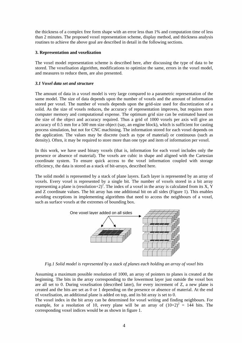
the thickness of a complex free form shape with an error less than 1% and computation time of less than 2 minutes. The proposed voxel representation scheme, display method, and thickness analysis routines to achieve the above goal are described in detail in the following sections. 3. Representation and voxelization The voxel model representation scheme is described here, after discussing the type of data to be stored. The voxelisation algorithm, modifications to optimize the same, errors in the voxel model, and measures to reduce them, are also presented. 3.1 Voxel data set and structure The amount of data in a voxel model is very large compared to a parametric representation of the same model. The size of data depends upon the number of voxels and the amount of information stored per voxel. The number of voxels depends upon the grid-size used for discretization of a solid. As the size of voxels reduces, the accuracy of representation improves, but requires more computer memory and computational expense. The optimum grid size can be estimated based on the size of the object and accuracy required. Thus a grid of 1000 voxels per axis will give an accuracy of 0.5 mm for a 500 mm size object (say, an engine block), which is sufficient for casting process simulation, but not for CNC machining. The information stored for each voxel depends on the application. The values may be discrete (such as type of material) or continuous (such as density). Often, it may be required to store more than one type and item of information per voxel. In this work, we have used binary voxels (that is, information for each voxel includes only the presence or absence of material). The voxels are cubic in shape and aligned with the Cartesian coordinate system. To ensure quick access to the voxel information coupled with storage efficiency, the data is stored as a stack of bit-arrays, described here. The solid model is represented by a stack of plane layers. Each layer is represented by an array of voxels. Every voxel is represented by a single bit. The number of voxels stored in a bit array representing a plane is (resolution+2)2. The index of a voxel in the array is calculated from its X, Y and Z coordinate values. The bit array has one additional bit on all sides (Figure 1). This enables avoiding exceptions in implementing algorithms that need to access the neighbours of a voxel, such as surface voxels at the extremes of bounding box.

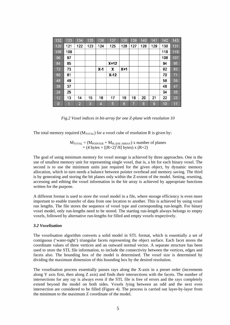
Fig.1 Solid model is represented by a stack of planes each holding an array of voxel bits Assuming a maximum possible resolution of 1000, an array of pointers to planes is created at the beginning. The bits in the array corresponding to the lowermost layer just outside the voxel box are all set to 0. During voxelisation (described later), for every increment of Z, a new plane is created and the bits are set as 0 or 1 depending on the presence or absence of material. At the end of voxelisation, an additional plane is added on top, and its bit array is set to 0. The voxel index in the bit array can be determined for voxel writing and finding neighbours. For example, for a resolution of 10, every plane will be an array of (10+2)2 = 144 bits. The corresponding voxel indices would be as shown in figure 1.

One voxel layer added on all sides

5

Fig.2 Voxel indices in bit-array for one Z-plane with resolution 10

The total memory required (MTOTAL) for a voxel cube of resolution R is given by:

MTOTAL = (MPOINTER + MPLANE ARRAY) x number of planes = (4 bytes + [(R+2)2/8] bytes) x (R+2)

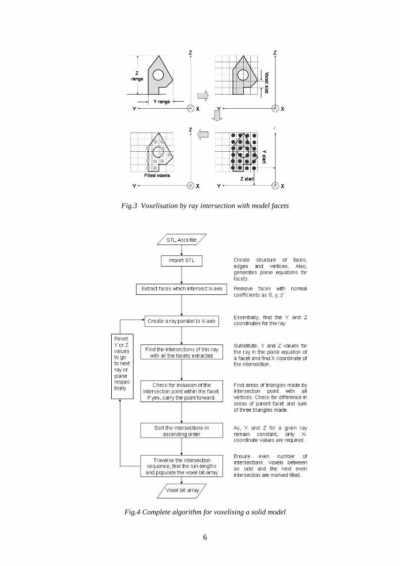
The goal of using minimum memory for voxel storage is achieved by three approaches. One is the use of smallest memory unit for representing single voxel, that is, a bit for each binary voxel. The second is to use the minimum units just required for the given object, by dynamic memory allocation, which in turn needs a balance between pointer overhead and memory saving. The third is by generating and storing the bit planes only within the Z-extent of the model. Setting, resetting, accessing and editing the voxel information in the bit array is achieved by appropriate functions written for the purpose. A different format is used to store the voxel model in a file, where storage efficiency is even more important to enable transfer of data from one location to another. This is achieved by using voxel run lengths. The file stores the sequence of voxel type and corresponding run-length. For binary voxel model, only run-lengths need to be stored. The starting run-length always belongs to empty voxels, followed by alternative run-lengths for filled and empty voxels respectively. 3.2 Voxelisation The voxelisation algorithm converts a solid model in STL format, which is essentially a set of contiguous (‘water-tight’) triangular facets representing the object surface. Each facet stores the coordinate values of three vertices and an outward normal vector. A separate structure has been used to store the STL file information, to include the connectivity between the vertices, edges and facets also. The bounding box of the model is determined. The voxel size is determined by dividing the maximum dimension of this bounding box by the desired resolution. The voxelisation process essentially passes rays along the X-axis in a preset order (increments along Y axis first, then along Z axis) and finds their intersections with the facets. The number of intersections for any ray is always even if the STL file is free of errors and the rays completely extend beyond the model on both sides. Voxels lying between an odd and the next even intersection are considered to be filled (Figure 4). The process is carried out layer-by-layer from the minimum to the maximum Z coordinate of the model.

6

Fig.3 Voxelisation by ray intersection with model facets

Fig.4 Complete algorithm for voxelising a solid model

7

The first ray originates from:

Y start = Yminimum of the model + (Voxel size / 2) Z start = Zminimum of the model + (Voxel size / 2)

Subsequent rays are passed at a distance equal to the voxel size along Y and Z axes. For each ray, the intersections are sorted in ascending order, and the run-lengths are determined as follows.

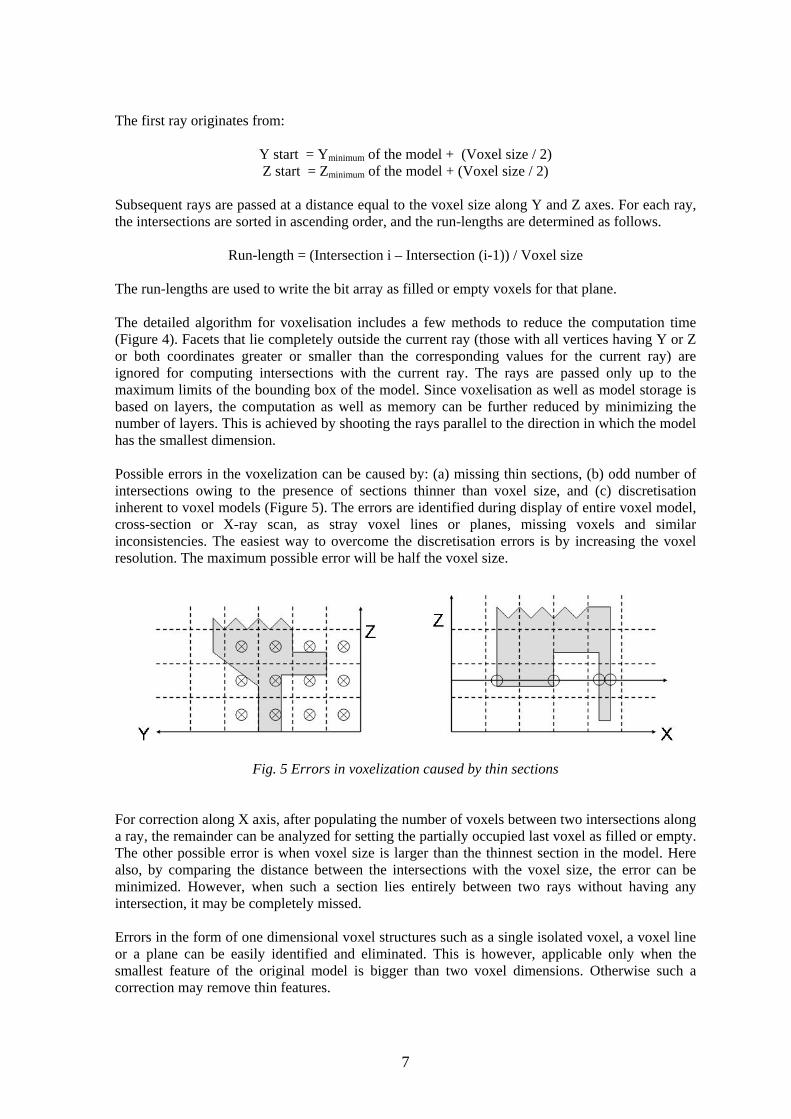
Run-length = (Intersection i – Intersection (i-1)) / Voxel size The run-lengths are used to write the bit array as filled or empty voxels for that plane. The detailed algorithm for voxelisation includes a few methods to reduce the computation time (Figure 4). Facets that lie completely outside the current ray (those with all vertices having Y or Z or both coordinates greater or smaller than the corresponding values for the current ray) are ignored for computing intersections with the current ray. The rays are passed only up to the maximum limits of the bounding box of the model. Since voxelisation as well as model storage is based on layers, the computation as well as memory can be further reduced by minimizing the number of layers. This is achieved by shooting the rays parallel to the direction in which the model has the smallest dimension. Possible errors in the voxelization can be caused by: (a) missing thin sections, (b) odd number of intersections owing to the presence of sections thinner than voxel size, and (c) discretisation inherent to voxel models (Figure 5). The errors are identified during display of entire voxel model, cross-section or X-ray scan, as stray voxel lines or planes, missing voxels and similar inconsistencies. The easiest way to overcome the discretisation errors is by increasing the voxel resolution. The maximum possible error will be half the voxel size.

Fig. 5 Errors in voxelization caused by thin sections

For correction along X axis, after populating the number of voxels between two intersections along a ray, the remainder can be analyzed for setting the partially occupied last voxel as filled or empty. The other possible error is when voxel size is larger than the thinnest section in the model. Here also, by comparing the distance between the intersections with the voxel size, the error can be minimized. However, when such a section lies entirely between two rays without having any intersection, it may be completely missed. Errors in the form of one dimensional voxel structures such as a single isolated voxel, a voxel line or a plane can be easily identified and eliminated. This is however, applicable only when the smallest feature of the original model is bigger than two voxel dimensions. Otherwise such a correction may remove thin features.

8

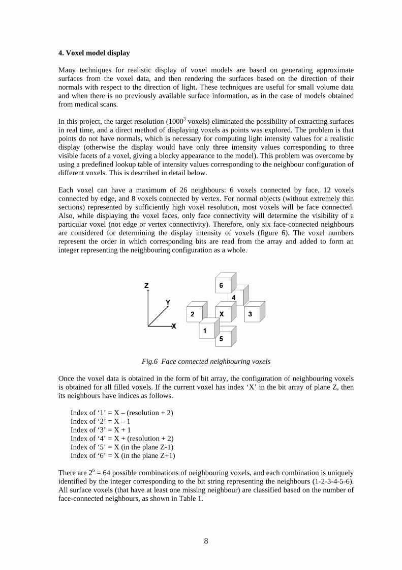
4. Voxel model display Many techniques for realistic display of voxel models are based on generating approximate surfaces from the voxel data, and then rendering the surfaces based on the direction of their normals with respect to the direction of light. These techniques are useful for small volume data and when there is no previously available surface information, as in the case of models obtained from medical scans. In this project, the target resolution (10003 voxels) eliminated the possibility of extracting surfaces in real time, and a direct method of displaying voxels as points was explored. The problem is that points do not have normals, which is necessary for computing light intensity values for a realistic display (otherwise the display would have only three intensity values corresponding to three visible facets of a voxel, giving a blocky appearance to the model). This problem was overcome by using a predefined lookup table of intensity values corresponding to the neighbour configuration of different voxels. This is described in detail below. Each voxel can have a maximum of 26 neighbours: 6 voxels connected by face, 12 voxels connected by edge, and 8 voxels connected by vertex. For normal objects (without extremely thin sections) represented by sufficiently high voxel resolution, most voxels will be face connected. Also, while displaying the voxel faces, only face connectivity will determine the visibility of a particular voxel (not edge or vertex connectivity). Therefore, only six face-connected neighbours are considered for determining the display intensity of voxels (figure 6). The voxel numbers represent the order in which corresponding bits are read from the array and added to form an integer representing the neighbouring configuration as a whole.

Fig.6 Face connected neighbouring voxels Once the voxel data is obtained in the form of bit array, the configuration of neighbouring voxels is obtained for all filled voxels. If the current voxel has index ‘X’ in the bit array of plane Z, then its neighbours have indices as follows.

Index of ‘1’ = X – (resolution + 2) Index of ‘2’ = X – 1 Index of ‘3’ = X + 1 Index of ‘4’ = X + (resolution + 2) Index of ‘5’ = X (in the plane Z-1) Index of ‘6’ = X (in the plane Z+1)

There are 26 = 64 possible combinations of neighbouring voxels, and each combination is uniquely identified by the integer corresponding to the bit string representing the neighbours (1-2-3-4-5-6). All surface voxels (that have at least one missing neighbour) are classified based on the number of face-connected neighbours, as shown in Table 1.

9

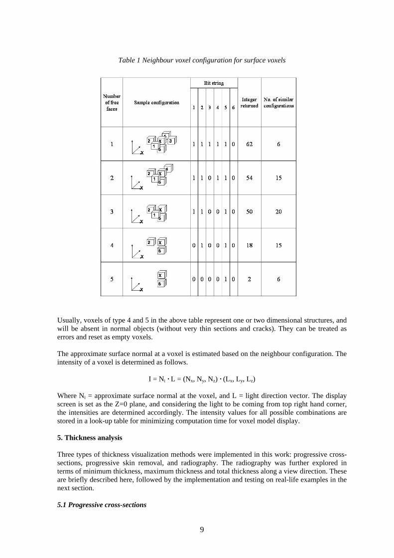
Table 1 Neighbour voxel configuration for surface voxels

Usually, voxels of type 4 and 5 in the above table represent one or two dimensional structures, and will be absent in normal objects (without very thin sections and cracks). They can be treated as errors and reset as empty voxels. The approximate surface normal at a voxel is estimated based on the neighbour configuration. The intensity of a voxel is determined as follows.

I = Ni · L = (Nx, Ny, Nz) · (Lx, Ly, Lz)

Where Ni = approximate surface normal at the voxel, and L = light direction vector. The display screen is set as the Z=0 plane, and considering the light to be coming from top right hand corner, the intensities are determined accordingly. The intensity values for all possible combinations are stored in a look-up table for minimizing computation time for voxel model display. 5. Thickness analysis Three types of thickness visualization methods were implemented in this work: progressive cross-sections, progressive skin removal, and radiography. The radiography was further explored in terms of minimum thickness, maximum thickness and total thickness along a view direction. These are briefly described here, followed by the implementation and testing on real-life examples in the next section. 5.1 Progressive cross-sections

10

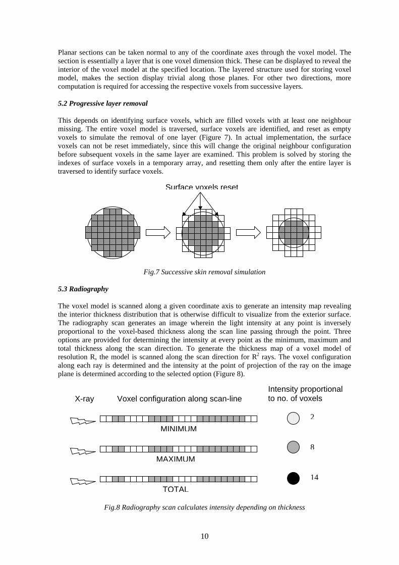
Planar sections can be taken normal to any of the coordinate axes through the voxel model. The section is essentially a layer that is one voxel dimension thick. These can be displayed to reveal the interior of the voxel model at the specified location. The layered structure used for storing voxel model, makes the section display trivial along those planes. For other two directions, more computation is required for accessing the respective voxels from successive layers. 5.2 Progressive layer removal This depends on identifying surface voxels, which are filled voxels with at least one neighbour missing. The entire voxel model is traversed, surface voxels are identified, and reset as empty voxels to simulate the removal of one layer (Figure 7). In actual implementation, the surface voxels can not be reset immediately, since this will change the original neighbour configuration before subsequent voxels in the same layer are examined. This problem is solved by storing the indexes of surface voxels in a temporary array, and resetting them only after the entire layer is traversed to identify surface voxels.

Fig.7 Successive skin removal simulation

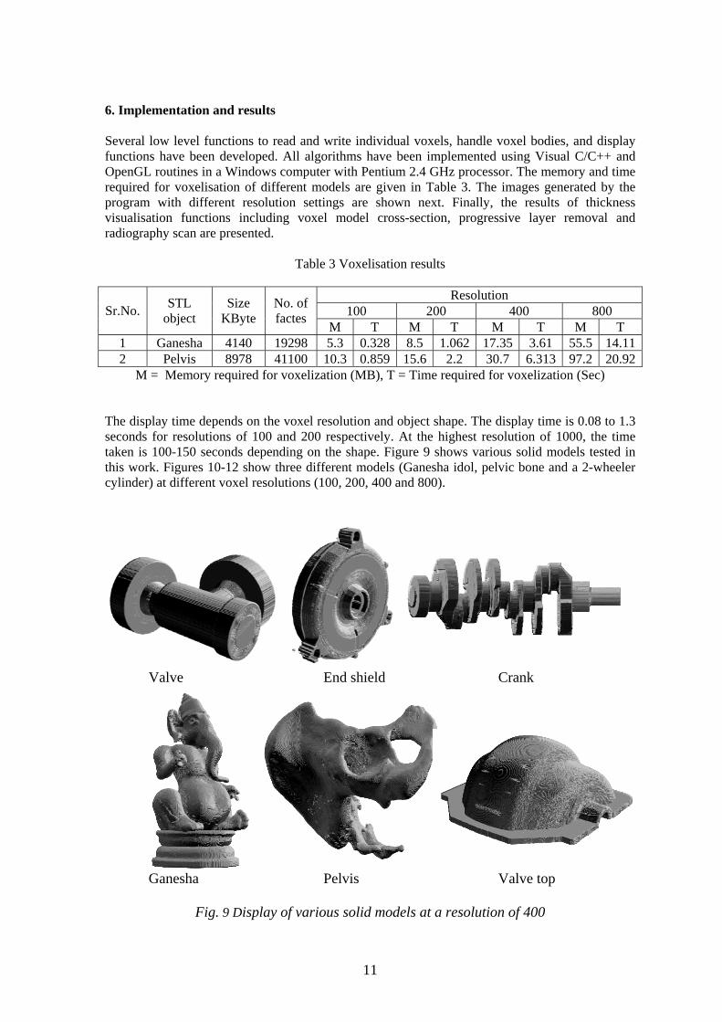
5.3 Radiography The voxel model is scanned along a given coordinate axis to generate an intensity map revealing the interior thickness distribution that is otherwise difficult to visualize from the exterior surface. The radiography scan generates an image wherein the light intensity at any point is inversely proportional to the voxel-based thickness along the scan line passing through the point. Three options are provided for determining the intensity at every point as the minimum, maximum and total thickness along the scan direction. To generate the thickness map of a voxel model of resolution R, the model is scanned along the scan direction for R2 rays. The voxel configuration along each ray is determined and the intensity at the point of projection of the ray on the image plane is determined according to the selected option (Figure 8).

Fig.8 Radiography scan calculates intensity depending on thickness

Surface voxels reset

Intensity proportional to no. of voxels X-ray Voxel configuration along scan-line

2

8

14

MINIMUM

MAXIMUM

TOTAL

11

6. Implementation and results Several low level functions to read and write individual voxels, handle voxel bodies, and display functions have been developed. All algorithms have been implemented using Visual C/C++ and OpenGL routines in a Windows computer with Pentium 2.4 GHz processor. The memory and time required for voxelisation of different models are given in Table 3. The images generated by the program with different resolution settings are shown next. Finally, the results of thickness visualisation functions including voxel model cross-section, progressive layer removal and radiography scan are presented.

Table 3 Voxelisation results

Resolution 100 200 400 800 Sr.No. STL

object Size

KByte No. of factes M T M T M T M T

1 Ganesha 4140 19298 5.3 0.328 8.5 1.062 17.35 3.61 55.5 14.112 Pelvis 8978 41100 10.3 0.859 15.6 2.2 30.7 6.313 97.2 20.92

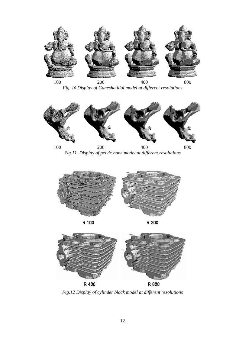
M = Memory required for voxelization (MB), T = Time required for voxelization (Sec) The display time depends on the voxel resolution and object shape. The display time is 0.08 to 1.3 seconds for resolutions of 100 and 200 respectively. At the highest resolution of 1000, the time taken is 100-150 seconds depending on the shape. Figure 9 shows various solid models tested in this work. Figures 10-12 show three different models (Ganesha idol, pelvic bone and a 2-wheeler cylinder) at different voxel resolutions (100, 200, 400 and 800).

Valve End shield Crank

Ganesha Pelvis Valve top

Fig. 9 Display of various solid models at a resolution of 400

12

100 200 400 800 Fig. 10 Display of Ganesha idol model at different resolutions

100 200 400 800 Fig.11 Display of pelvic bone model at different resolutions

Fig.12 Display of cylinder block model at different resolutions

13

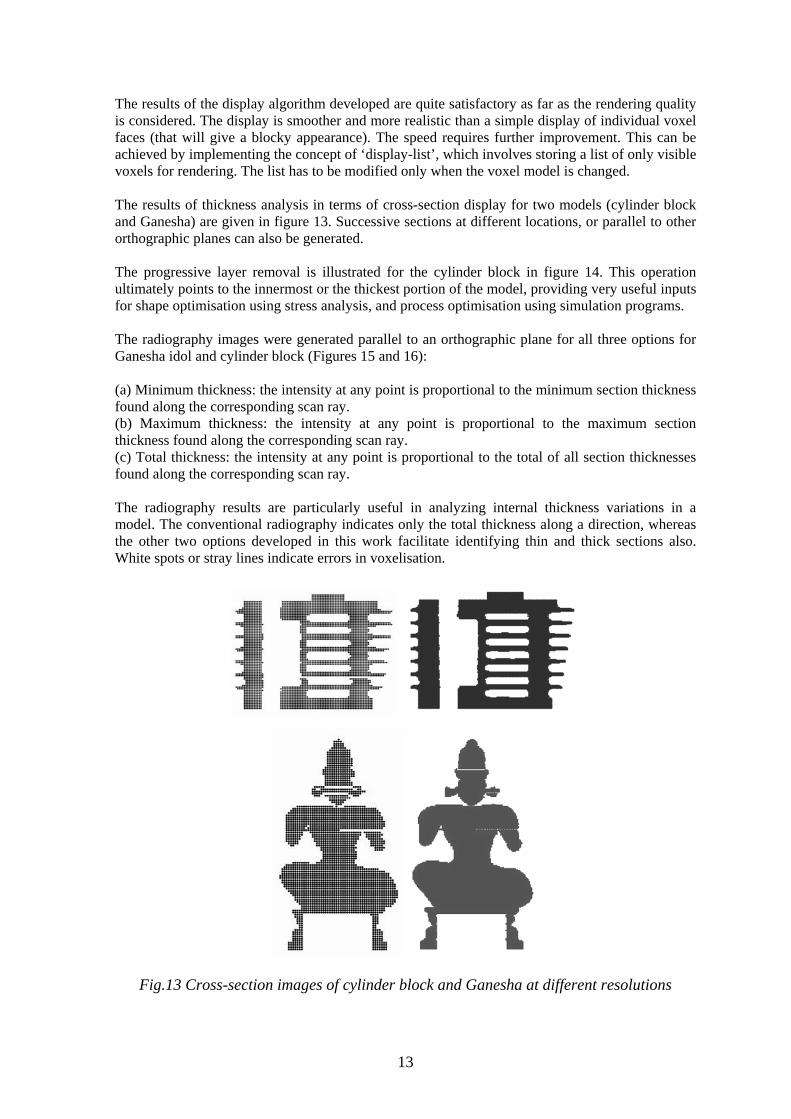
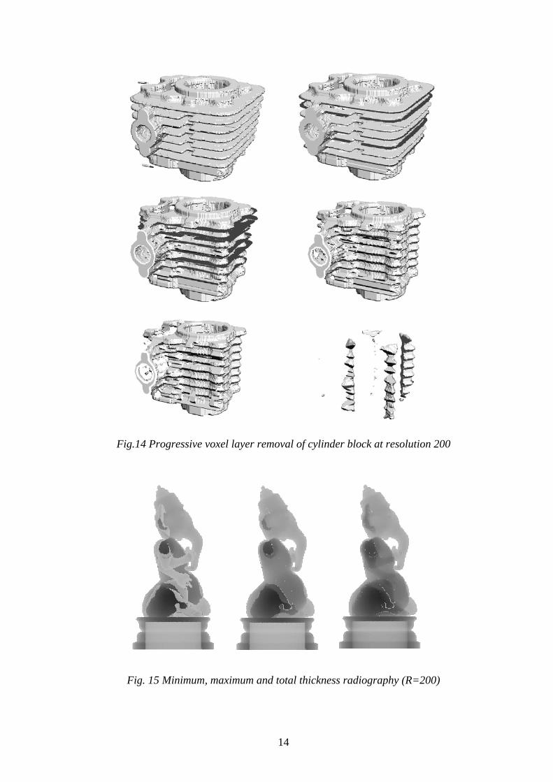
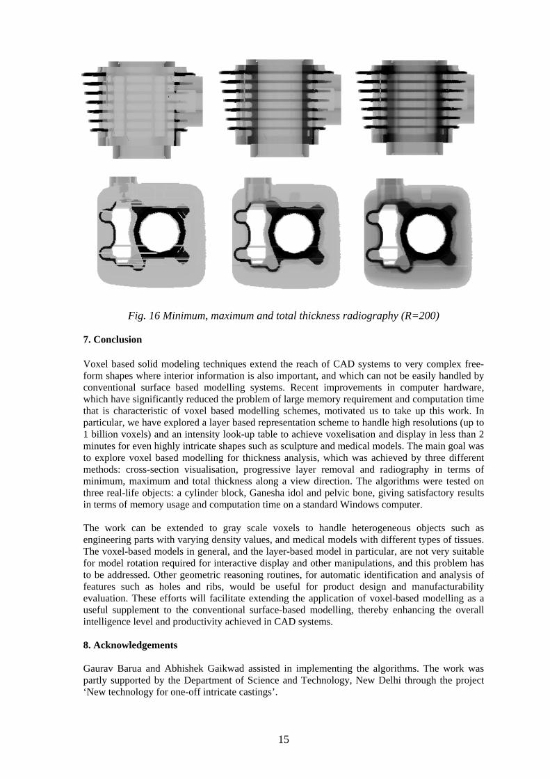
The results of the display algorithm developed are quite satisfactory as far as the rendering quality is considered. The display is smoother and more realistic than a simple display of individual voxel faces (that will give a blocky appearance). The speed requires further improvement. This can be achieved by implementing the concept of ‘display-list’, which involves storing a list of only visible voxels for rendering. The list has to be modified only when the voxel model is changed. The results of thickness analysis in terms of cross-section display for two models (cylinder block and Ganesha) are given in figure 13. Successive sections at different locations, or parallel to other orthographic planes can also be generated. The progressive layer removal is illustrated for the cylinder block in figure 14. This operation ultimately points to the innermost or the thickest portion of the model, providing very useful inputs for shape optimisation using stress analysis, and process optimisation using simulation programs. The radiography images were generated parallel to an orthographic plane for all three options for Ganesha idol and cylinder block (Figures 15 and 16): (a) Minimum thickness: the intensity at any point is proportional to the minimum section thickness found along the corresponding scan ray. (b) Maximum thickness: the intensity at any point is proportional to the maximum section thickness found along the corresponding scan ray. (c) Total thickness: the intensity at any point is proportional to the total of all section thicknesses found along the corresponding scan ray. The radiography results are particularly useful in analyzing internal thickness variations in a model. The conventional radiography indicates only the total thickness along a direction, whereas the other two options developed in this work facilitate identifying thin and thick sections also. White spots or stray lines indicate errors in voxelisation.

Fig.13 Cross-section images of cylinder block and Ganesha at different resolutions

14

Fig.14 Progressive voxel layer removal of cylinder block at resolution 200

Fig. 15 Minimum, maximum and total thickness radiography (R=200)

15

Fig. 16 Minimum, maximum and total thickness radiography (R=200) 7. Conclusion Voxel based solid modeling techniques extend the reach of CAD systems to very complex free-form shapes where interior information is also important, and which can not be easily handled by conventional surface based modelling systems. Recent improvements in computer hardware, which have significantly reduced the problem of large memory requirement and computation time that is characteristic of voxel based modelling schemes, motivated us to take up this work. In particular, we have explored a layer based representation scheme to handle high resolutions (up to 1 billion voxels) and an intensity look-up table to achieve voxelisation and display in less than 2 minutes for even highly intricate shapes such as sculpture and medical models. The main goal was to explore voxel based modelling for thickness analysis, which was achieved by three different methods: cross-section visualisation, progressive layer removal and radiography in terms of minimum, maximum and total thickness along a view direction. The algorithms were tested on three real-life objects: a cylinder block, Ganesha idol and pelvic bone, giving satisfactory results in terms of memory usage and computation time on a standard Windows computer. The work can be extended to gray scale voxels to handle heterogeneous objects such as engineering parts with varying density values, and medical models with different types of tissues. The voxel-based models in general, and the layer-based model in particular, are not very suitable for model rotation required for interactive display and other manipulations, and this problem has to be addressed. Other geometric reasoning routines, for automatic identification and analysis of features such as holes and ribs, would be useful for product design and manufacturability evaluation. These efforts will facilitate extending the application of voxel-based modelling as a useful supplement to the conventional surface-based modelling, thereby enhancing the overall intelligence level and productivity achieved in CAD systems. 8. Acknowledgements Gaurav Barua and Abhishek Gaikwad assisted in implementing the algorithms. The work was partly supported by the Department of Science and Technology, New Delhi through the project ‘New technology for one-off intricate castings’.

16

References [1] Acker, D.E., Sobierajski, L., Cohen, D., Kaufman, A., Yagel, R., “A fast display method for Volumetric data”, The Visual Computer: International Journal of Computer Graphics, Vol. 10, No. 2, pp.116-124, 1993. [2] Chandru, V., Manohar, S., and Prakash, C.E., “Voxel based Modeling for Layered Manufacturing”, IEEE Computer Graphics and Applications, Vol. 15, No. 6, pp. 42-47, Nov 1995. [3] Elvins, T.T., "A Survey of Algorithms for Volume Visualization", Computer Graphics, Vol. 26, No.3, pp. 194-201, 1992. [4] Fang, S., Liao, D., “Fast CSG Voxelization by Frame Buffer Pixel Mapping”, IEEE/ACM Proceedings of Volume Visualization and Graphics Symposium, Salt Lake City, UT, U.S.A., pp. 43-48, 2000. [5] Huang, J., Yagel, R., Filippov, V., Kurzion, Y., “An accurate method for voxelizing polygon meshes”, Proceedings of the 1998 IEEE symposium on Volume visualization, pp. 119-126, 1998. [6] Jense, G.J., “Voxel-based methods for CAD”, Computer-aided design, Vol. 21, No. 8, pp. 528-533, Oct 1989. [7] Jones, M.W., Satherley, R.A., “Shape representation using space filled sub-voxel distance fields”, International Conference on Shape Modeling and Applications, pp. 316-325, May 2001. [8] Kaufman, A., Shimony, E., “3D scan-conversion algorithms for voxel based graphics”, Proceedings of the 1986 workshop on Interactive 3D graphics, pp. 45-75, 1987. [9] Kaufman, A., Cohen, D. and Yagel, R., ‘‘Volume Graphics’’, IEEE Computer, Vol. 26, No. 7, pp. 51-64, July 1993. [10] Lu, S.C., Rebello, A.B., Cui, D.H., Yagel, R., Miller, R.A., Kinzel, G.L., “A Visualization Tool For Mechanical Design”, Proceedings of the 7th conference on Visualization, pp. 401-404, 1996. [11] Nooruddin, F. S., Turk, G., “Simplification and Repair of Polygonal Models Using Volumetric Techniques”, IEEE Transactions on Visualization and Computer Graphics, Vol. 9, No. 2, pp. 191-205, April-June 2003. [12] Prakash, C.E., Nandy, S.K., “Voxel based modeling and rendering irregular solids”, Microprocessing and Microprogramming, Vol. 30, No. 1-5, pp. 341-346 , Aug 1990. [13] Wang, S.W., Kaufman, A.E., “Volume sampled voxelization of geometric primitives”, Proceedings of the 4th conference on Visualization, pp. 78-84, 1993. [14] Yagel, R., Lu, S.C., Rebello, A.B., Miller, R.A., “Volume based reasoning and visualization of Diecastability”, Proceedings of the 6th conference on Visualization, pp. 359-362, 1995.