Voronoi diagram generation on the ellipsoidal earth

Hai Hu a, XiaoHang Liu b,n, Peng Hu a,c

a College of Resources and Environmental Science, Wuhan University, 129 LuoYu Road, Wuhan 430079, PR Chinab Department of Geography and Environment, San Francisco State University, 1600 Holloway Avenue, San Francisco, CA 94132, USAc College of Resources and Environmental Engineering, Anhui University, 111 Jiulong Road, Hefei 230601, PR China

a r t i c l e i n f o

Article history:Received 21 January 2014Received in revised form21 August 2014Accepted 26 August 2014Available online 16 September 2014

Keywords:Voronoi diagramDistance transformGeographical distanceEarth ellipsoid

a b s t r a c t

Voronoi diagram on the earth surface is a powerful tool to study spatial proximity at continental orglobal scale. However, its computation remains challenging because geospatial features have complexshapes. This paper presents a raster-based algorithm to generate Voronoi diagrams on earth's surface.The algorithm approximates the exact point-to-point geographical distances using the cell-to-cellgeographical distances calculated by a geographical distance transform. The result is a distance imageon which Voronoi diagram is delineated. Compared to existing methods, the proposed algorithmcalculates geographical distances based on an earth ellipsoid and allows Voronoi generators to takecomplex shapes. Most importantly, its approximation error is bounded thus enabling users to control theaccuracy of the Voronoi diagram through grid resolution.

& 2014 Elsevier Ltd. All rights reserved.

1. Introduction

Voronoi diagram, which is also called Thiessen polygon orDirichlet tessellation, is a powerful tool to study spatial proximityor regions of influence of a set of features (called Voronoigenerators). It partitions the space into regions such that all pointsin the region centered around a feature are closer to it than to anyother feature (Aurenhammer, 1991). Voronoi diagram is used invarious disciplines such as meteorology, forestry, chemistry,archeology, and biology (Okabe et al., 2000). In the context ofgeography and geosciences, Voronoi diagram has been applied tolocation allocation of facilities (Iri et al., 1984), earthquake dis-tribution analysis (Nicholson et al., 2000), rainfall-runoff modeling(Tucker and Lancaster, 2001), 3D volumetric reconstruction ofgeological objects (Courrioux et al., 2001), uncertainties in reser-voir modeling (Subbeya et al., 2004), errors in remotely sensedimagery interpretation (Nelson et al., 2005), seismic tomography(Zhang and Thurber, 2005), population landscape (Mu and Wang,2006), and multi-resolution climate system modeling (Ringleret al., 2008). In addition to proximity analysis, Voronoi diagramand its dual are a promising data structure to build a dynamicgeographical information systems (GIS) to handle global georefer-enced data (Gold, 1991; Gahegan and Lee, 2000; Beni et al., 2011),it is thus studied intensively in the context of discrete global gridsystem (Sahr et al., 2003).

Compared to other disciplines, Voronoi diagram generation inearth science has two main challenges. The first is how to measurethe distance between geospatial features. Technically, geospatialfeatures are located on the earth, thus their proximity should bemeasured along earth's surface. In reality, the study area is usuallyprojected from earth to a map using an appropriate map projec-tion, Voronoi diagram generation is conducted on the map usingplanar distances such as Euclidean distance, city-block distance, orchessboard distance. Challenges emerge when a research is atcontinental or global scale which is often the case in this age ofglobalization. No map projection can preserve distances at theglobal scale, thus distance must be measured directly along thesurface of earth. To date, substantial research has been conductedon how to generate Voronoi diagrams on a plane. In contrast, howto generate Voronoi diagrams on the ellipsoidal earth is much lessstudied.

In addition to distance calculation, the shape of geospatialfeatures is another challenge to Voronoi diagram generation.Geospatial features often have complex shapes. Taking a coastlineas an example, it may be in the form of an extended polyline orcurve (e.g. US coastline in the Gulf of Maine), a set of disjointpolygons (e.g. the Philippine Archipelago), or a compound madeup by disjoint points, lines, and polygons (e.g. a main coastline andseveral offshore islands and rocks). In fact, the shape of a coastlineis almost impossible to anticipate because it changes with geo-graphical scale. A small island may be simplified to a single pointat a small geographical scale, but becomes a polygon or even a setof polygons at a larger scale. This suggests that, in order togenerate a Voronoi diagram based on geospatial features, themethod used must allow Voronoi generators in complex shapes.

Contents lists available at ScienceDirect

journal homepage: www.elsevier.com/locate/cageo

Computers & Geosciences

http://dx.doi.org/10.1016/j.cageo.2014.08.0110098-3004/& 2014 Elsevier Ltd. All rights reserved.

n Corresponding author.E-mail addresses: huhai@whu.edu.cn (H. Hu), xhliu@sfsu.edu (X. Liu),

penghu@whu.edu.cn (P. Hu).

Computers & Geosciences 73 (2014) 81–87

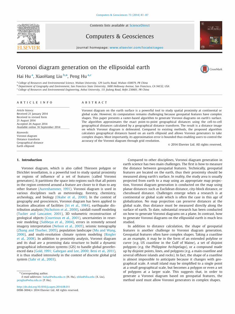
This paper examines how to address aforementioned two chal-lenges simultaneously, i.e. Voronoi diagram generation on the ellip-soidal earth based on Voronoi generators in any arbitrary shape. Inthe literature, both raster and vector approaches have been explored.Vector approaches are often found in computational geometry underthe theme of Voronoi diagram on a polyhedral surface (Okabe et al.,2000) or spherical Voronoi diagram (Miles, 1971; Brown, 1980). Whenthe Voronoi generators are points, the insertion method byAugenbaum and Peskin (1985), the incremental method by Renka(1997), and the method to generate spherical centroidal Voronoidiagrams by Du et al. (2003) can be used. If the Voronoi generatorsare circles or circular arcs, the algorithms by Sugihara (2002) and Naet al. (2002) are applicable. It has to be noted that most of the vector-based methods developed are for spherical Voronoi diagrams onlywhile the earth is typically referred to as a reference ellipsoid in earthscience. Fig. 1 is an illustration of the Voronoi diagram based on 228world capital cities. World Geodetic System 1984 datum is used tomodel the earth ellipsoid (Preschern, 2012).

In geoscience, raster-based Voronoi diagram generation is impor-tant because many geospatial data are routinely acquired by photo-grammetry and remote sensing. This is especially true when aresearch is at continental or global scale, a circumstance wheregeographical distance must be used. Data extracted from photogram-metry and remote sensing are often distributed as a grid. Raster-based Voronoi diagram generation works with grid data directly,avoiding raster-to-vector conversions which can be error prone andtime consuming if the dataset is large and complex. Another benefitof raster-based approach is that a complex shape can be easilyapproximated by a set of cells. This is especially advantageous if ageospatial feature is made up by a set of disjoint features. Ingeoscience and GIS, raster-based approach has been explored mostly

for planar Voronoi diagrams (e.g. Li et al., 1999; Dong, 2008). TheO-QTM (Octahedral Quaternary Triangular Mesh) by Chen et al.(2003) seems the only raster-based exploration to generate Voronoidiagrams on earth. This method tessellates earth's surface hierarchi-cally using spherical facets based on Octahedrons so that sphericalcoordinates can be linked to triangle address codes. Distance on thequaternary triangular mesh (QTM), i.e. QTM distance, is then calcu-lated using mathematical morphology. Spherical (not ellipsoidal)Voronoi diagram based on QTM distance is computed as an approx-imate of the exact Voronoi diagram on earth. The main challenge tothis algorithm is its accuracy, as the approximation error is notconstant but depends on the location. There does not exist a boundfor this approximation error, nor there exists a mechanism to allowusers to control this error.

This paper presents a new raster-based exploration to generateVoronoi diagrams on the earth. Unlike previous research, thealgorithm models the earth as an ellipsoid and allows thegenerators to have any shape. In the following sections, we firstprovide a definition of raster-based Voronoi diagram based ongeographical distance, then presents geographical distance trans-form which is key to generating Voronoi diagrams on the earthellipsoid. This is followed by an analysis of the accuracy, efficiency,and limitation of the algorithm.

2. Voronoi diagram based on geographical distance

In geoscience, earth is described by a geodetic datum such asWorld Geodetic System (WGS) 1984 or North American Datum(NAD) 1983. A geodetic datum models earth using a referenceellipsoid, e.g. the Geodetic Reference System (GRS) 1980 which has

Fig. 1. Voronoi diagram based on the capitals of 228 countries and territories on a WGS84 ellipsoid (Preschern, 2012).

H. Hu et al. / Computers & Geosciences 73 (2014) 81–8782

a semi-major axis of 6378137.0 m and an inverse flattening of298.257. Geographical distance is calculated based on the refer-ence ellipsoid. If a geospatial feature is a point, its distance toanother point is the point-to-point geographical distance, i.e. theshortest path along the surface of the reference ellipsoid at sealevel. If a geospatial featuregi is not a point, but a line, a polygon, ora complex shape, its geographical distance to a point q is definedas the minimum distance between q and a point q0in gi, i.e.

dGðq; giÞ ¼ min fdGðq; q0Þjq0Agig ð1ÞIf q is part ofgi, i.e.qAgi, then dGðq; giÞ equals 0. Superscript G is

used to denote geographical distance, as d alone typically refers toplanar distance in the literature.

Based on Eq. (1), a Voronoi diagram using geographical dis-tance can be defined as follows. Supposing G¼ fg1; g2;…gng is a setof geospatial features on the ellipsoidal earth, each feature is calleda Voronoi generator and has an arbitrary shape. Let q be a point.The dominance of generator gi over generator gj, called RðgijgjÞ, isdefined as

RðgijgjÞ ¼ fpjdGðp; giÞrdGðp; gjÞ; giAG; gjAG; ia jg ð2Þ

The Voronoi region of gi, denoted by VðgiÞ, is made up by pointswhose distance to giis shorter than to any other Voronoi generator,i.e.

VðgiÞ ¼ \gi AG;gj A fG�gig

RðgijgjÞ

The Voronnoi diagram of Gis defined as

VðGÞ ¼ [gi AG

VðgiÞ

It can be seen that the key to generating Voronoi diagrams onan earth ellipsoid is the computation of point-to-point geographi-cal distances. Exact point-to-point distance on an ellipsoid canonly be obtained using mathematical equations. In practicalapplications, Vincente's (1975) inverse distance formula is oftenused because it is very efficient and extremely accurate (Thomasand Featherstone, 2005). Details of this formula are provided inAppendix A. In this paper, we use the point-to-point distanceobtained by Vincente's inverse distance formula as the referenceto evaluate the accuracy of our raster-based algorithm.

3. Rationale of raster-based Voronoi diagram generation

Rigorously speaking, exact Voronoi diagrams as defined by Eq. (2)can only be obtained by vector methods where space is infinitelydiscernible and each point is referenced by its coordinates. In raster-based Voronoi generation, space is modeled by a grid and cell is theelementary unit. A point has to be approximated by a cell and aVoronoi generator has to be approximated by a set of cells. As aresult, the point-to-generator distance in Eq. (1) must be calculatedas the cell-to-generator distance which is the minimum geographicaldistance from the cell to any cell in the generator. In this paper, wedefine cell-to-cell distance as the geographical distance betweentheir centroids. Apparently, a cell-to-cell distance in raster space isnot exactly the same as a point-to-point distance in vector space.A raster Voronoi diagram is therefore only an approximation of theexact Voronoi diagram. Nevertheless, an approximation is stillvaluable because geoscience applications can usually tolerate a smallamount of errors. The key is to assure that the error is under controland within the tolerance threshold.

Let p and q be two points on the earth ellipsoid; dGðp; qÞdenotes their geographical distance computed using Vincente'sinverse formula. When a raster-based method is used, p and qaremapped to grid cells and they are referred to by the centroid of thecorresponding cells. Assuming the centroids are p0 and q0

respectively, dGðp; qÞ is approximated by the geographical distancebetween p0 and q0, i.e. dGðp0; q0Þ. This approximation introduces anerror as illustrated in Fig. 2. However, if each cell is small enoughthat the curvature of the earth within a cell can be ignored, theerror is bounded by

ffiffiffi

2p

r where r is the spatial resolution of thegrid, i.e.

jdGðp; qÞ�dGðp0; q0Þjrffiffiffi

2p

r ð3ÞIn practical applications, an area less than 20 km in extent is

generally considered flat. Thus, as long as each cell is less than20 km in extent which is very easy to satisfy in geoscienceapplications, point-to-point vector distance can be approximatedby cell-to-cell raster distance with a bounded error of

ffiffiffi

2p

r. Eq. (3)establishes the rationale on using raster-based methods to approx-imate exact vector-based Voronoi diagrams. It can be seen that theapproximation accuracy depends on the grid resolution (r). Thesmaller is r, the smaller is the approximation error. Note the errorbound of

ffiffiffi

2p

r is based on the condition that the exact value ofdGðp0; q0Þ is available. How to obtain exact dGðp0; q0Þ, i.e. cell-to-celldistance, is thus the key challenge to raster-based Voronoi diagramgeneration. Previous research such as Chen et al. (2003) was notable to solve this challenge. In this paper, we present geographicaldistance transform as a solution.

4. Voronoi diagram generation

4.1. Geographical distance transform

Section 3 demonstrates that raster-based methods can approx-imate the exact vector-based Voronoi diagram with controlledaccuracy, provided that the raster-based method is able to produceexact cell-to-cell geographical distances. One way to obtain theexact cell-to-cell geographical distance is to use Vincente's inversedistance formula directly, but this crude calculation is extremelytime-consuming. Instead, this research develops a geographicaldistance transform which calculates geographical distances fastand effectively. Distance transform is intensively studied in imageprocessing and pattern recognition (Borgefors, 1986). Given abinary image where the foreground is Voronoi generators andthe background is the rest of the image, distance transformcomputes two new images. One is called distance image wherethe value of each pixel is its distance to the nearest foregroundpixel (or equivalently Voronoi generator); the other, which storesthe identifier of the nearest foreground pixel of each pixel, is calledgenerator image in this paper. Conceptually, distance transform isbased on distance propagation which is similar to the buffering orwaterlining process – buffers are generated from each foregroundpixel and the buffer fronts keep proceeding until they meet eachother or the boundary of the study area is reached. The pixelswhere buffer fronts meet form Voronoi boundaries.

Fig. 2. Relationship between vector- and raster-based distances.

H. Hu et al. / Computers & Geosciences 73 (2014) 81–87 83

Existing research on distance transform is mainly based on planardistances especially Euclidean distance (Fabbri et al., 2008). Oneestablished methodology is to use a two-scan propagation scheme toupdate distance values iteratively (Cuisenaire and Macq, 1999; Shihand Wu, 2004). This methodology is modified to implement geo-graphical distance transform. Assuming a study area is bounded byλminrλrλmaxin latitude and φminrφrφmax in longitude, the firststep is to project the study area to a map. Any projection can be usedas long as it guarantees a one-to-one correspondence between alatitude–longitude coordinate ðλ;φÞ and a Cartesian coordinate (x,y).For illustration purposes, this paper uses cylindrical equidistantprojection. If the reference ellipsoid has a radius of R, the followingrelationship exists:

x¼ Rðφ�φ0Þ y¼ Rλ ð4Þ

where φ0 is the longitude of the central meridian. Equivalently,there is

λ¼ y=R φ¼ φ0þx=R ð5Þ

Using Eq. (4), a study area bounded by λminrλrλmax andφminrφrφmax on earth surface can be projected to a rectangularregion bounded by xminrxrxmax and yminryrymax on a cylind-rical equidistant map. Similarly, a rectangular region on a cylindricalequidistant map can be mapped to the earth surface using Eq. (5).

Once the study area is projected from the earth ellipsoid to acylindrical equidistant map, the next step is to overlay a grid of Mcolumns and N rows on the map. The values of M andN depend onthe spatial resolution ðrÞ of the grid. Each point ðx; yÞ on thecylindrical equidistance map falls in a grid cell ði; jÞ where i and jare row and column index respectively. Assuming the centroid ofthe lower left cell is (xmin ;ymin), the centroid of cell ði; jÞ, denotedby ðxc; ycÞ, can be obtained by

xc ¼ xminþ ir yc ¼ yminþ jr; ð6Þ

ðxc; ycÞ is a coordinate on the cylindrical equidistant map. It canbe mapped to the earth ellipsoid using Eq. (5). In this way, thecorrespondence between a latitude–longitude coordinate ðλ;φÞ, aCartesian coordinateðx; yÞ, and a cell ði; jÞ is established. Geogra-phical distance transform proceeds as follows:

Step 1: Create an image where the foreground is the Voronoigenerators and the background is the other pixels. Initialize thedistance map by assigning the value of pixel ði; jÞ, denoted as Dij,as follows: if ði; jÞ is a foreground pixel, Dij is 0; Otherwise, Dij isa sufficiently large value K .Step 2: Sweep the image forwardly and update the value ofeach pixel using its neighbors in Fig. 3, i.e.

for ði¼ 0; ioM; iþþÞfor ðj¼ 0; joN; jþþÞ

Dij ¼ min fDij;Rijðq1Þ;Rijðq2Þ;Rijðq3Þ;Rijðq4Þg

Step 3: Sweep the image in reverse order and update the valueof each pixel using its neighbors in Fig. 3

for ði¼M�1; iZ0; i��Þfor ðj¼N�1; jZ0; j��Þ

DGij ¼ min fDij;Rijðq5Þ;Rijðq6Þ;Rijðq7Þ;Rijðq8Þg

In Step 2 and Step 3, RijðqÞ; q¼ q1…q8 is the geographicaldistance between pixel ði; jÞ and the nearest foreground pixel ofits neighbor q during that iteration. To calculate RijðqÞ, the

Cartesian coordinates ðxi; yjÞ of each pixel's centroid is found firstusing Eq. (6); ðxi; yjÞ is then mapped to a point ðλ1;φ1Þ on the earthsurface using Eq. (5). By the same token, the nearest foregroundpixel of q is mapped to a point ðλ2;φ2Þ. The geographical distancebetween ðλ1;φ1Þ and ðλ2;φ2Þ is then calculated using Vincente'sinverse distance formula to result in RijðqÞ.

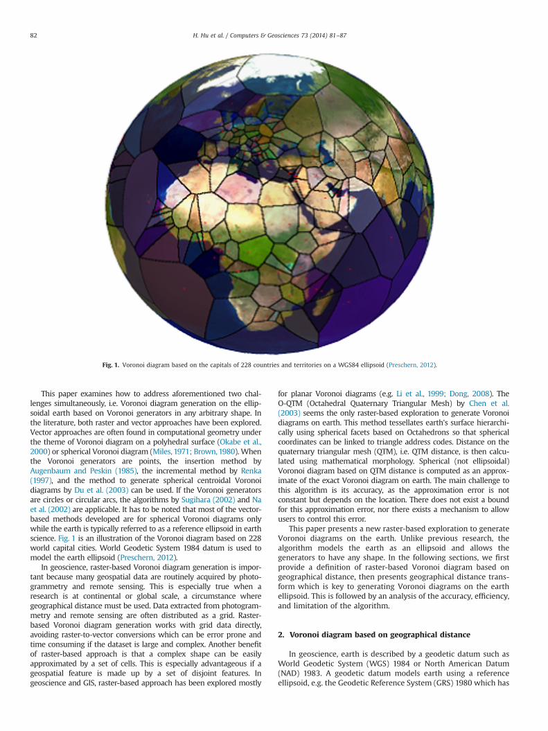
Step 2 and Step 3 usually involve four neighbors except for pixelslocated at image border. For these boundary pixels, only the applic-able neighbors are used. Fig. 4 illustrates how the algorithm proceedsduring forward and backward scan. Fig. 4a is the result after forwardscan, Fig. 4b is the result after backward scan. The values in Fig. 4 aresquared geographical distance which is identical to squared Euclideandistance because the area in Fig. 4 is so small that the curvature of theearth does not have any impact. In practical applications, geographicaldistance transform always returns geographical distance which istypically a floating-point number. One may consider rounding thefloating point values to integers to obtain an integer distance image.This will introduce a rounding error of no more than 0.5, but theinteger image obtained is much easier to handle than the originalfloating-point distance image in terms of storage, symbolization, andvisualization.

4.2. Voronoi boundary delineation

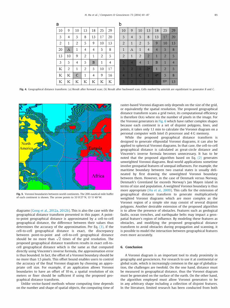
Once the distance image and the generator image are obtained,Voronoi boundaries can be delineated based on the distance imageby tracing pixels whose distance is higher than or equal to all of itsneighbors. Alternatively, if a pixel does not have the same nearestgenerator as its neighbors, this pixel must be on a Voronoiboundary. Fig. 5 is an example where world continents are usedas Voronoi generators. Each continent is made up by a set ofdisjoint polygons, lines, and/or points. A 200-nautical mile bufferis drawn for each continent based on the distance image. Thelocation pointed to by the arrow is 33 30027″N, 13 311049″W .

Fig. 6 is created by overlaying the Voronoi boundaries with themid-ocean ridges depicted in Grotelüschen (1970). All continentsare assigned equal weights. It is interesting to notice the coin-cidence between Voronoi boundaries and mid-ocean ridges insome parts of the earth. Plate tectonics theory suggests that mid-ocean ridges were created by convection currents cracking acontinent plate and pushing the broken halves apart. The distanceof a mid-ocean ridge to the continents may thus help infer theforces involved. How findings like Fig. 6 can be used to assistresearch in earth science is beyond the scope of this paper.However, this example illustrates the necessity to computeVoronoi diagrams on the surface of the earth.

5. Discussion

As discussed in Section 2, exact Voronoi diagram can only beobtained through exact computational geometry. Most methodsincluding vector methods only produce approximate Voronoi

Fig. 3. The neighborhood of a pixel.

H. Hu et al. / Computers & Geosciences 73 (2014) 81–8784

diagrams (Gong et al., 2012a, 2012b). This is also the case with thegeographical distance transform presented in this paper. A point-to-point geographical distance is approximated by a cell-to-cellgeographical distance, the difference between their values thusdetermines the accuracy of the approximation. Per Eq. (3), if thecell-to-cell geographical distance is exact, the discrepancybetween point-to-point and cell-to-cell geographical distanceshould be no more than

ffiffiffi

2p

times of the grid resolution. Theproposed geographical distance transform results in exact cell-to-cell geographical distance which is the same as that computeddirectly using Vincente's inverse formula, the approximation erroris thus bounded. In fact, the offset of a Voronoi boundary should beno more than 1.5 pixels. This offset bound enables users to controlthe accuracy of the final Voronoi diagram by choosing an appro-priate cell size. For example, if an application allows Voronoiboundaries to have an offset of 10 m, a spatial resolution of sixmeters or finer should be sufficient if using the proposed geo-graphical distance transform.

Unlike vector-based methods whose computing time dependson the number and shape of spatial objects, the computing time of

raster-based Voronoi diagram only depends on the size of the grid,or equivalently the spatial resolution. The proposed geographicaldistance transform scans a grid twice, its computational efficiencyis therefore OðnÞ where nis the number of pixels in the image. Forthe Voronoi generators in Fig. 6 which have rather complex shapesbecause each continent is a set of disjoint polygons, lines, andpoints, it takes only 1.1 min to calculate the Voronoi diagram on apersonal computer with Intel i5 processor and 4 G memory.

While the proposed geographical distance transform isdesigned to generate ellipsoidal Voronoi diagrams, it can also beapplied to spherical Voronoi diagrams. In that case, the cell-to-cellgeographical distance is calculated as great-circle distance andVincente's inverse formula becomes unnecessary. It has to benoted that the proposed algorithm based on Eq. (2) generatesunweighted Voronoi diagrams. Real-world applications sometimeinvolve geospatial features of unequal influences. For example, themaritime boundary between two coastal states is usually deli-neated by first drawing the unweighted Voronoi boundarybetween them. However, in the case of Denmark versus Norway,Denmark's Greenland far exceeds Norway's Jan Mayen island interms of size and population. A weighted Voronoi boundary is thusmore appropriate (Hu et al., 2009). This calls for the extension ofgeographical distance transform to generate multiplicativelyweighted Voronoi diagrams which are more complex as theVoronoi region of a simple site may consist of several disjointpolygons. Another desirable extension of the proposed algorithmis to allow the presence of obstacles. Features such as geologicalfaults, ocean trenches, and earthquake belts may impact a geos-patial feature's region of influence. By modeling these features asobstacles, and modifying the proposed geographical distancetransform to avoid obstacles during propagation and scanning, itis possible to model the interaction between geographical featureseven more accurately.

6. Conclusion

A Voronoi diagram is an important tool to study proximity ingeography and geosciences. For research to use it at continental orglobal scale, which is increasingly common in the age of globaliza-tion, the challenges are twofold. On the one hand, distance mustbe measured in geographical distance, thus the Voronoi diagrammust be generated on the surface of the earth. On the other hand,the algorithm employed must allow Voronoi generators to bein any arbitrary shape including a collection of disjoint features.In the literature, limited research has been conducted from both

Fig. 4. Geographical distance transform: (a) Result after forward scan; (b) Result after backward scan. Cells marked by asterisk are equidistant to generator B and C.

Fig. 5. Voronoi boundaries between world continents. The 200-nautical mile bufferof each continent is shown. The arrow points to 3310027″N, 13111049″W.

H. Hu et al. / Computers & Geosciences 73 (2014) 81–87 85

the vector and the raster perspective. While vector-based methodsare able to create exact Voronoi diagrams, its complexity increasesrapidly as Voronoi generators become more complex. In contrast,raster-based methods can model a complex shape easily but theVoronoi diagram generated is only an approximation of the exactVoronoi diagram. The ability of a raster-based method to controlthe approximation accuracy is thus critical. In this paper, we havepresented a raster-based method based on geographical distancetransform to compute Voronoi diagrams on the ellipsoidal earth.Unlike existing raster-based methods, the approximation error inthe proposed method is bounded thus enabling users to achievetheir desired accuracy by choosing an appropriate grid resolution.In the future, the proposed algorithm may be extended to allowgenerators of varying weights as well as the presence of obstacleson the earth.

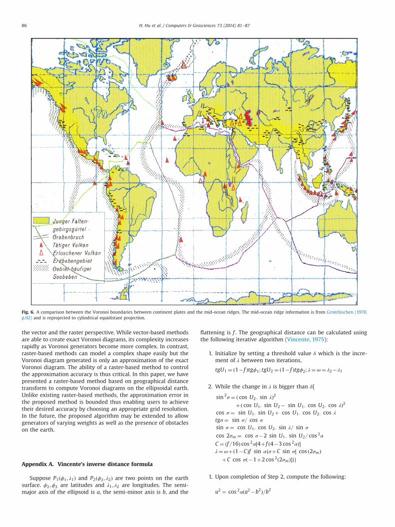
Appendix A. Vincente's inverse distance formula

Suppose P1ðϕ1; λ1Þ and P2ðϕ2; λ2Þ are two points on the earthsurface. ϕ2;ϕ2 are latitudes and λ1; λ2 are longitudes. The semi-major axis of the ellipsoid is a, the semi-minor axis is b, and the

flattening is f . The geographical distance can be calculated usingthe following iterative algorithm (Vincente, 1975):

1. Initialize by setting a threshold value δ which is the incre-ment of λ between two iterations,

tgU1 ¼ ð1� f Þtgϕ1; tgU2 ¼ ð1� f Þtgϕ2; λ¼ ω¼ λ2�λ1

2. While the change in λ is bigger than δ{

sin 2σ ¼ ð cos U2: sin λÞ2þð cos U1: sin U2� sin U1: cos U2: cos λÞ2

cos σ ¼ sin U1: sin U2þ cos U1: cos U2: cos λ

tgσ ¼ sin σ= cos σ

sin σ ¼ cos U1: cos U2: sin λ= sin σ

cos 2σm ¼ cos σ�2 sin U1: sin U2= cos 2α

C ¼ ðf =16Þ cos 2α½4þ f ð4�3 cos 2αÞ�λ¼ ωþð1�CÞf sin αfσþC sin σ½ cos ð2σmÞ

þC cos σð�1þ2 cos 2ð2σmÞ�gg

1. Upon completion of Step 2, compute the following:

u2 ¼ cos 2αða2�b2Þ=b2

Fig. 6. A comparison between the Voronoi boundaries between continent plates and the mid-ocean ridges. The mid-ocean ridge information is from Grotelüschen (1970,p.92) and is reprojected to cylindrical equidistant projection.

H. Hu et al. / Computers & Geosciences 73 (2014) 81–8786

A¼ 1þðu2=16384Þf4096þu2½�768þu2ð320�175u2Þ�gB¼ ðu2=1024Þf256þu2½�128þu2ð74�47u2Þ�gΔσ ¼ B sin σf cos 2σmþðB=4Þ½ cos αð�1þ2 cos 22σmÞ

�ðB=6Þ cos 2σmð�3þ4 sin 2σÞð�3þ4 cos 22σmÞ�g

The geographical distance between P1 and P2 is

dGðP1; P2Þ ¼ Abðσ�ΔσÞ

References

Augenbaum, J., Peskin, C., 1985. On the construction of the Voronoi meshes on asphere. J. Computational Phys. 59, 177–192.

Aurenhammer, F., 1991. Voronoi diagrams: a survey of a fundamental geometricdata structure. ACM Comput. Surv. 23, 345–405.

Beni, L.H., Mostafavi, M.A., Pouliot, J., Gavrilova, M., 2011. Toward 3D spatialdynamic field simulation within GIS using kinetic Voronoi diagram andDelauney tetrahedralization. Int. J. Geograp. Inform. Sci. 25 (1), 25–50.

Borgefors, G., 1986. Distance transformations in digital images. Comput. Vis. Graph.Image Process. 34, 344–371.

Brown, K., 1980. Geometric transforms for fast geometric algorithms (Ph. D. Thesis,Report CMU-CS-80-101). Carnegie-Mellon University, Pittsburgh, PA.

Chen, J., Zhao, X., Li, Z., 2003. An algorithm for the generation of Voronoi diagramson the sphere based on QTM. Photogramm. Eng. Remote Sens. 69 (1), 79–89.

Courrioux, G., Nullans, S., Guillen, A., Boissonnat, J.D., Repusseau, P., Renaud, X.,Thibaut, M., 2001. 3D volumetric modeling of Cadomian terranes (NorthernBrittany, France): an automatic method using Voronoı diagrams. Tectonophy-sics 331 (1), 181–196.

Cuisenaire, O., Macq, B., 1999. Fast Euclidean distance transformation by propaga-tion using multiple neighborhoods. Comput. Vis. Image Underst. 76 (2),163–172.

Dong, P., 2008. Generating and updating multiplicatively weighted Voronnoidiagrams for point, line and polygon features in GIS. Comput. Geosci. 34 (4),411–421.

Du, Q., Gunzburger, M., Ju, L., 2003. Constrained centroidal Voronoi tessellations forsurfaces. SIAM J. Sci. Comput. 24, 1488–1506.

Fabbri, R., Costa Luciano Da, F., Torelli, J.C., Bruno, O., 2008. 2D Euclidean distancetransform algorithms: a comparative survey. ACM Comput. Surv. 40 (1), 2.

Gahegan, M., Lee, I., 2000. Data structures and algorithms to support interactivespatial analysis using dynamic Voronoi diagrams. Comput. Environ. Urban Syst.24 (6), 509–537.

Gold, C., 1991. Problems with handling spatial data – the Voronoi approach. Can.Instit. Surv. Mapp. J. 45, 65–80.

Gong, Y., Li, G., Tian, Y., Lin, Y., Liu, Y., 2012a. A vector-based algorithm to generateand update multiplicatively weighted Voronoi diagrams for points, polylines,and polygons. Comput. Geosci. 42, 118–125.

Gong, Y., Wu, L., Lin, Y., Liu, Y., 2012b. Probability issues in locality descriptionsbased on Voronoi neighbor relationship. J. Visual Lang. Comput. 23, 213–222.

Grotelüschen, W., 1970. Unsere Welt, Atlas. Geographische VerlagsgesellschaftVelhagen & Klasing und Hermann Schroedel, Berlin: Germany p. 179 (p. p.92).

Hu, H., Yang, C., Hu, P., 2009. Methods to delimit median line and proportional lineamong features in complex shapes. Mar. Surv. 5, 15–20 (In Chinese).

Iri, M., Murota, K., Ohya, T., 1984. A fast Voronoi-diagram algorithm with applica-tions to geographical optimization problems. Syst. Model. Optim. Lect. NotesControll. Inform. Sci. 59, 273–288.

Li, C., Chen, J., Li, Z., 1999. A raster-based method for computing Voronoi diagramsof spatial objects using dynamic distance transformation. Int. J. Geogr. Inform.Sci. 13 (3), 209–225.

Miles, R.E., 1971. Random points, sets and tessellations on the surface of a sphere.Sankhya (Indian J. Stat.), Series A 33, 145–174.

Mu, L., Wang, X., 2006. Population landscape: a geometric approach to studyingspatial patterns of the US urban hierarchy. Int. J. Geogr. Inform. Sci. 20 (6),649–667.

Na, H., Lee, C., Cheong, O., 2002. Voronoi diagram on the sphere. ComputationalGeom. 23, 183–194.

Nelson, T., Boots, B., Wulder, M., 2005. Techniques for accuracy assessment of treelocations extracted from remotely sensed imagery. J. Environ. Manage. 74 (3),265–271.

Nicholson, T., Sambridge, M., Gudmundsson, Ó., 2000. On entropy and clustering ofearthquake hypocentre distributions. Geophys. J. Int. 142 (1), 37–51.

Okabe, A, Boots, B., Sugihara, K., Chiu, S.N., 2000. Spatial Tessellations: Concepts andapplications of Voronoi diagrams, 2nd edition John Wiley & Sons, Chichester, UK.

Preschern, K. 2012. Voronoi diagram on the sphere. Available online ⟨http://www.preschern.org/detri/DeTri_en.html⟩, (accessed on 24.6.2014).

Renka, R.J. 1997. Algorithm 772: STRIPACK: Delaunay triangulation and Voronoidiagram on the surface of a sphere. ACM Transactions on MathematicalSoftware.

Ringler, T., Ju, L., Gunzburger, M., 2008. A multiresolution method for climatesystem modeling: application of spherical centroidal voronoi tessellations.Ocean Dynam. 58, 475–498.

Sahr, K., White, D., Kimerling, A.J., 2003. Geodesic discrete global grid systems.Cartogr. Geograph. Inform. Sci. 30 (2), 121–134.

Shih, F.Y., Wu, Y., 2004. Fast Euclidean distance transformation in two scans using a3�3 neighborhood. Comput. Vis. Image Underst. 93, 195–205.

Subbeya, S., Christiea, M., Sambridge, M., 2004. Prediction under uncertainty inreservoir modeling. J. Pet. Sci. Eng. 44, 143–153.

Sugihara, K., 2002. Laguerre Voronoi diagram on the sphere. J. Geom. Graph. 6 (1),69–81.

Thomas, C, Featherstone, W, 2005. Validation of Vincenty's formulas for thegeodesic using a new fourth-order extension of Kivioja's formula. J. Surv. Eng.131, 20–26.

Tucker, G.E., Lancaster, S.T., 2001. An object-oriented framework for distributedhydrologic and geomorphic modeling using triangulated irregular networks.Comput. Geosci. 27 (8), 959–973.

Vincente, T., 1975. Direct and inverse solutions of geodesics on the Ellipsoid withapplications of nested equations. Surv. Rev. 23 (176), 88–93.

Zhang, H., Thurber, C., 2005. Adapative mesh seismic tomography basedon tetrahedral and Voronoi Diagrams: application to parkfield, California.J. Geophys. Res. B: Solid Earth 110 (4), 1–13.

H. Hu et al. / Computers & Geosciences 73 (2014) 81–87 87