Volume 3 An Efficient Thermal Infrared Radiation ...f NASA Technical Memorandum 104606, Vol. 3...
98
f NASA Technical Memorandum 104606, Vol. 3 Technical Report Series on Global Modeling and Data Assimilation Max J. Suarez, Editor Goddard Space Flight Center Greenbelt, Maryland Volume 3 An Efficient Thermal Infrared Radiation Parameterization for Use in General Circulation Models Ming-Dah Chou Max J. Suarez Goddard Space Flight Center Greenbelt, Maryland National Aeronautics and Space Administration Goddard Space Flight Center Greenbelt, Maryland 1994 https://ntrs.nasa.gov/search.jsp?R=19950009331 2020-04-04T19:45:54+00:00Z
Transcript of Volume 3 An Efficient Thermal Infrared Radiation ...f NASA Technical Memorandum 104606, Vol. 3...
f
NASA Technical Memorandum 104606, Vol. 3
Technical Report Series on
Global Modeling and Data Assimilation
Max J. Suarez, Editor
Goddard Space Flight Center
Greenbelt, Maryland
Volume 3
An Efficient Thermal Infrared Radiation
Parameterization for Use in General
Circulation Models
Ming-Dah Chou
Max J. Suarez
Goddard Space Flight Center
Greenbelt, Maryland
National Aeronautics andSpace Administration
Goddard Space Flight CenterGreenbelt, Maryland1994
https://ntrs.nasa.gov/search.jsp?R=19950009331 2020-04-04T19:45:54+00:00Z

71 ;I i ;

Abstract
A detailed description of a parameterization for thermal infrared radiative transfer
designed specifically for use in global climate models is presented. The parameteri-cation includes the effects of the main absorbers of terrestrial radiation: water vapor,
carbon dioxide, and ozone. While being computationally efficient, the schemes compute
very accurately the clear-sky fluxes and cooling rates from the earth's surface to 0.01
mb. Errors are < 0.4 K day -1 in the cooling rate and < 1% in the fluxes. Since no
transmittances are pre-computed, the atmospheric layers and the vertical distribution
of the absorbers may be freely specified. The scheme can also account for any verticaldistribution of fractional cloudiness with arbitrary optical thickness. In addition, the
numerics and the FORTRAN implementation have been carefully designed to conserve
both memory and computer time. This code should thus be particularly attractive
to those contemplating long-term climate simulations, wishing to model the middle
atmosphere, or planning to use a large number of levels in the vertical.
oo,
111 PAGli BLa.NK NOT FILMED1
PA'C,E.____I INTENTIOt_LLY _L_,I_

Contents
List of Figures
List of Tables
1 Introduction
2 Infrared Transfer Equations
2.1 Kadiative Transfer Through a Clear Atmosphere ...............
2.2 The Effects of Clouds ..............................
2.3 The Flux Calculation ...............................
3 Broad-Band Calculations
3.1 The 8 Bands ...................................
3.2 Planck-Weighted Band Integrals ........................
3.3 Band-Integrated Planck Functions .......................
4 Transmission Functions
vii
ix
6
6
8
10
10
4.1 The k-Distribution Method ........................... 11
4.2 Pre-Computed Transmittance Tables ...................... 15
4.3 One-Parameter Scaling For Water Vapor Continuum Absorption ...... 16
4.4 Overlapping of Absorptions ........................... 18
4.5 Special Treatment of the 15 #m Band ..................... 19
5 Vertical Discretization 22
6 Comparisons With Line-by-Line Calculations 25
PAGE B_).r_ I_T FIlJ_E)
PA'_]...... INi EN! iO,,',tA[L7 5JJ _'_,

7 Summary 30
Appendix A: Band-by-Band Reults 32
Appendix B: The Code 42
7.1 Subroutine IRRAD ................................ 43
7.2 Subroutine COLUMN .............................. 56
7.3 Subroutine TABLUP ............................... 58
7.4 Subroutine WVKDIS ............................... 61
7.5 Subroutine CO2KDIS .............................. 65
7.6 Subroutine H2OEXPS .............................. 67
7.7 Subroutine CONEXPS .............................. 70
7.8 Subroutine C02EXPS .............................. 72
7.9 Sample Program ................................. 75
7.10 Verification Output of Sample Program .................... 79
References 82
vi
List of Figures
4
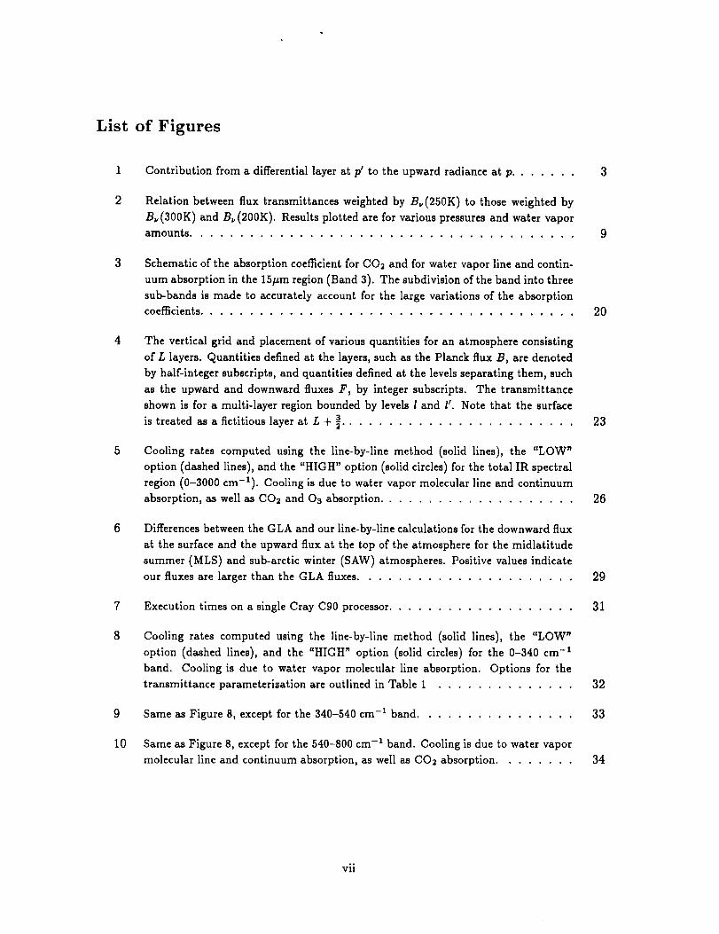
Contribution from a differential layer at p_ to the upward radiance at p .......
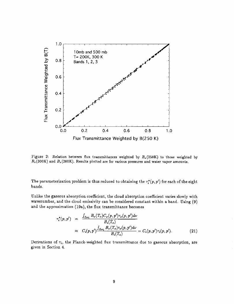
Relation between flux transmittances weighted by B_(250K) to those weighted by
B_(300K) and B_(200K). Results plotted are for various pressures and water vapor
amounts .......................................
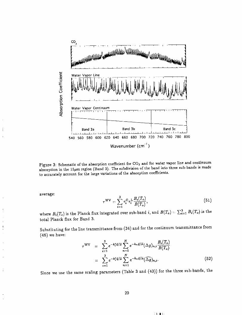
Schematic of the absorption coefficient for CO2 and for water vapor line and contin-
uum absorption in the 15/_m region (Band 3). The subdivision of the band into three
sub-bands is made to accurately account for the large variations of the absorption
coefficients ......................................
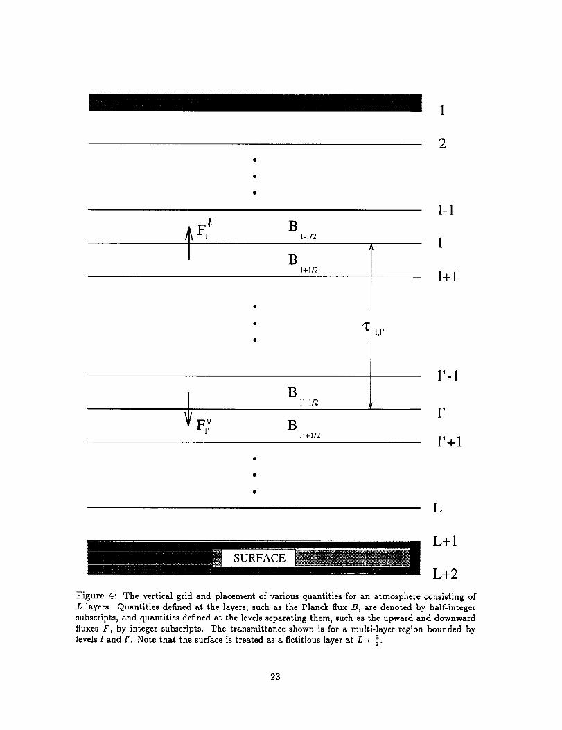
The vertical grid and placement of various quantities for an atmosphere consisting
of L layers. Quantities defined at the layers, such as the Planck flux B, are denoted
by half-integer subscripts, and quantities defined at the levels separating them, such
as the upward and downward fluxes F, by integer subscripts. The transmittance
shown is for a multi-layer region bounded by levels I and 1_. Note that the surface
is treated as a fictitious layer at L + _ ........................
Cooling rates computed using the line-by-line method (solid lines), the "LOW"
option (dashed lines), and the "HIGH" option (solid circles) for the total IR spectral
region (0-3000 cm-1). Cooling is due to water vapor molecular line and continuum
absorption, as well as CO2 and Os absorption ....................
Differences between the GLA and our line-by-line calculations for the downward flux
at the surface and the upward flux at the top of the atmosphere for the midlatitude
summer (MLS) and sub-arctic winter (SAW) atmospheres. Positive values indicate
our fluxes are larger than the GLA fluxes ......................
Execution times on a single Cray C90 processor ...................
Cooling rates computed using the line-by-line method (solid lines), the "LOW"
option (dashed lines), and the "HIGH" option (solid circles) for the 0-340 cm -1
band. Cooling is due to water vapor molecular line absorption. Options for the
transmittance parameterization are outlined in Table 1 ..............
9 Same as Figure 8, except for the 340-540 cm -I band ................
10 Same as Figure 8, except for the 540-800 cm -I band. Cooling is due to water vapor
molecular line and continuum absorption, as well as CO2 absorption ........
3
9
2O
23
26
29
31
32
33
34
vii

11
12
13
14
15
Same as Figure 8, except for the 800-980 cm-1 band. Cooling is due to water vapormolecular line and continuum absorption. Note that the HIGH and LOW options
are identical in this band ..............................
Same as Figure 8, except for the 980-1100 cm -t band. Cooling is due to water
vapor molecular line and continuum absorption, as well as 03 absorption ......
Same as Figure 8, except for the 1100-1380 cm -1 band. Cooling is due to water
vapor molecular line and continuum absorption ...................
Same as Figure 8, except for the 1380-1900 cm -1 band ...............
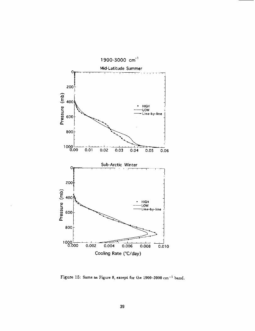
Same as Figure 8, except for the 1900-3000 cm -1 band ...............
35
36
37
38
39
.°.
Vlll
:i |f_
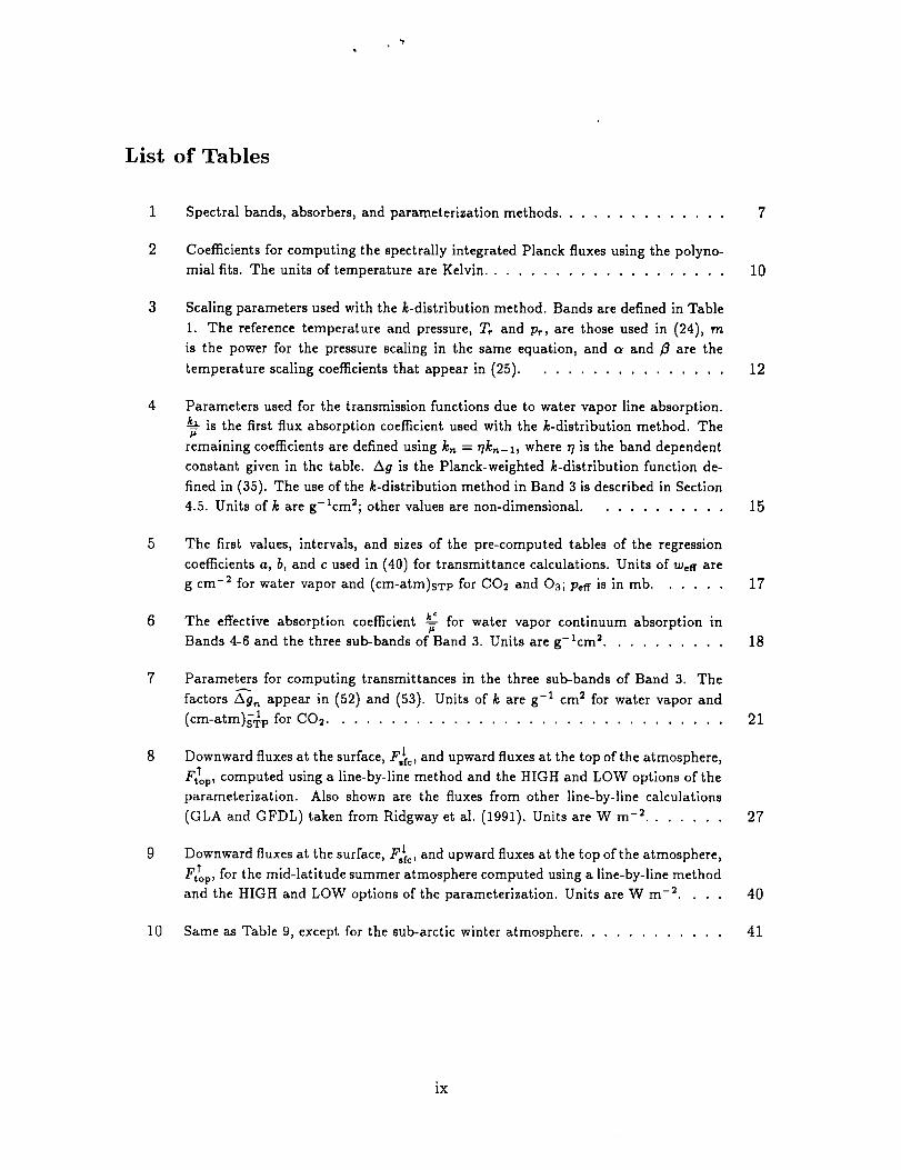
List of Tables
Spectral bands, absorbers, and parameterization methods ..............
Coefficients for computing the spectrally integrated Planck fluxes using the polyno-
mial fits. The units of temperature are Kelvin ....................
Scaling parameters used with the k-distribution method. Bands are defined in Table
1. The reference temperature and pressure, T, and p_, are those used in (24), m
is the power for the pressure scaling in the same equation, and a and _ are the
temperature scaling coefficients that appear in (25) ................
Parameters used for the transmission functions due to water vapor line absorption.
is the first flux absorption coeffÉcient used with the k-distribution method. The
remaining coefficients are defined using k,_ = T/k,_-l, where 77is the band dependent
constant given in the table. A 9 is the Planck-weighted k-distribution function de-
fined in (35). The use of the k-distribution method in Band 3 is described in Section
4.5. Units of k are g-lcm_; other values are non-dimenslonal ...........
The first values, intervals, and sizes of the pre-computed tables of the regression
coefficients a, b, and c used in (40) for transmittance calculations. Units of weft are
gcm -2 for water vapor and (cm-atm)sTP for CO2 and O3; P, fr is in mb ......
_c
The effective absorption coefficient _- for water vapor continuum absorption in
Bands 4-6 and the three sub-bands of Band 3. Units are g-lcm2 ..........
Parameters for computing transmittances in the three sub-bands of Band 3. The
factors A9, _ appear in (52) and (53). Units of k are g-1 cm 2 for water vapor and
(cm-atm)s_p for COs ................................
Downward fluxes at the surface, F_c , and upward fluxes at the top of the atmosphere,
Ft_op, computed using a line-by-line method and the HIGH and LOW options of the
parameterization. Also shown are the fluxes from other line-by-line calculations
(GLA and GFDL) taken from Ridgway et al. (1991). Units are W m -_ .......
Downward fluxes at the surface, F l and upward fluxes at the top of the atmosphere,sfc '
FtTop, for the mid-latitude summer atmosphere computed using a line-by-line method
and the HIGH and LOW options of the parameterization. Units are W m -2 ....
10 Same as Table 9, except for the sub-arctic winter atmosphere ............
10
12
15
17
18
21
27
40
41
ix

"VIV

1 Introduction
Thermal infrared radiation (IR) plays a crucial role in determining the earth's climate and
its sensitivity. It is, therefore, important to have an accurate IR radiation parameterization
in atmospheric general circulation models (GCMs) used for studying climate change. In
GCMs, calculations of thermal infrared fluxes can easily take a third or more of the com-
puting time. As the spatial resolution and vertical extent of the models increase and the
treatment of physical processes improves, it becomes imperative to have a fast and accurate
IP_ radiation parameterization.
Detailed calculation of the Il_ fluxes involves three integrations: a spectral integration, a
vertical integration, and a directional integration. The spectral integration is the most
time consuming. This is due to the narrowness of molecular absorption lines, which makes
the absorption coefficient vary rapidly with wavenumber and thus requires very high spec-
tral resolution (_ l0 s intervals for the entire II_ spectrum) to obtain accurate integrated
fluxes. But even this obstacle could be easily surmounted if it were not for the vertical
integration. If the atmosphere were vertically homogeneous in pressure and temperature,
the absorption coefficient over any vertical extent would be a function only of wavenumber,
and wavenumbers with the same absorption coefficient would be radiatively identical. The
spectral integration could then be greatly simplified by grouping all those spectral region
with the same absorption coefficient--the k-distribution approach (see, for example, Arkingand Grossman 1972). In the real atmosphere, however, the dependence of the absorption co-
efficient on pressure and temperature varies with wavenumber, and no two spectral intervals
can be treated identically. It is this difficulty that makes the broad-band parameterization
of IR fluxes such a difficult problem.
The effect of vertical variations of pressure and temperature on absorption is commonly
taken into account by using one of the following approximations:
One-parameter scaling, in which the effect of the variations of temperature and pres-
sure along a path are taken into account by reducing a nonhomogeneous layer to
an equivalent homogeneous layer with a "scaled" absorber amount at fixed reference
temperature and pressure (e.g., Chou and Arking 1980).
Two-parameter scaling, in which the effects of variations of temperature and pressure
along a path are taken into account by approximating a nonhomogeneous layer as a
homogeneous layer with the actual absorber amount, but at an effective temperature
and an effective pressure that depend on vertical variations within the layer (e.g.,
Kratz and Cess,1988; Chou and Kouvaris 1991; Schwarzkopf and Fels 1991; Morcrette
et al 1986; Kratz et al. 1993; Rosenfield 1991). In some cases (e.g., Schwarzkopf and
Fels 1991; Rogers and Walshaw 1966), effective optical properties, such as line width
and strength, are used as parameters instead of effective temperature and pressure; but
the objective is the same--to account for vertical inhomogeneities in the atmosphere.
• Modified k-distribution methods, in which, as in the traditional k-distribution ap-
proach, wavenumbers with similar absorption coefficient are grouped, but in such a
way as to account for the effects of vertical variations of temperature and pressure
(Chou et al. 1993; Fu and Liou 1992; Goody et al. 1989; Lacis and Oinas 1991; Wang
and Shi 1988; Zhu 1992).
At the Goddard Climate and Radiation Branch, we have developed various broad-band IR
radiation parameterizations for the major water vapor, carbon dioxide, and ozone absorption
bands based on all three approximations (Chou and Kouvaris 1991; Chou et al. 1993; Chou
et al. 1994). These IR radiation parameterizations have been shown to be accurate and
efficient in computing cooling rates in the troposphere and lower stratosphere, as well as in
the middle atmosphere (up to the 0.01-mb level).
This report describes in detail how these parameterizations have been integrated into a
single IR radiation package for use in GCMs. This package has been implemented andtested in the Goddard GCMs and is currently being used for both climate modeling and
data assimilation applications. In Section 2 we briefly review the transfer equations for fluxes
and cooling rates in clear and cloudy atmospheres. Section 3 addresses the partitioning of
the spectrum into broad bands and the representations of the spectrally integrated fluxes in
these bands. The forms of the transmittances used and the scheme for overlapping gaseous
absorptions are given in Section 4. The vertical discretization of the transfer equations is
given in Section 5. Section 6 presents some results of flux and cooling rate calculations and
compares the parameterization against line-by-line calculations. The results are summarized
in Section 7.
2 Infrared Transfer Equations
2.1 Radiative Transfer Through a Clear Atmosphere
Let us consider a thin atmospheric layer at pressure p' with a temperature T _, which has a
differential pressure thickness dp _ and an optical thickness du_, at wavenumber u (Figure 1).
The radiance emitted by this layer is n fT'_d_ where # is the cosine of the angle between
the beam and the vertical, and B,,(T _) is the Planck function. Let us further consider a
higher level at pressure p where we wish to compute the upweUing radiance, and let us
assume that between p and p_ there is a mixture of gaseous absorbers with monochromatic
optical thicknessg, I= p ), (1)
i
2
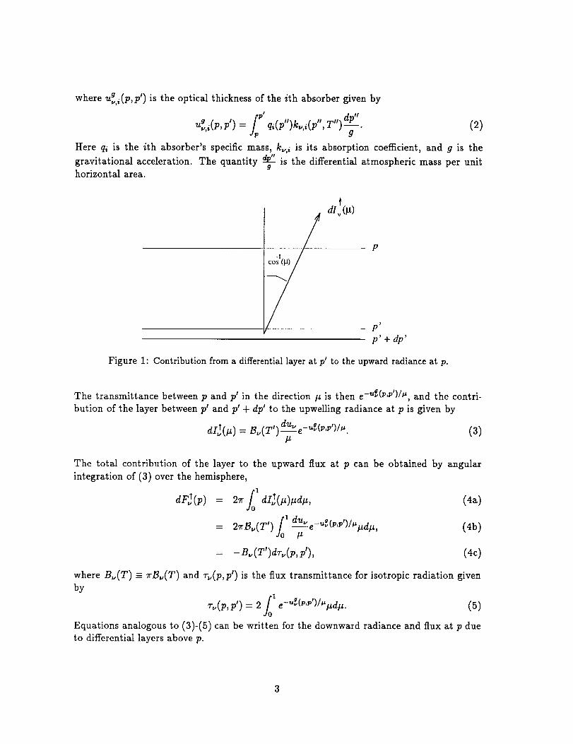
where guv,,(p, p ) is the optical thickness of the ith absorber given by
u_,,(p, p') = j!" q,(p")k_,,i(p", T H) dp".g (2)
Here qi is the ith absorber's specific mass, k_,, is its absorption coefficient, and g is the
gravitational acceleration. The quantity _ is the differential atmospheric mass per unitghorizontal area.
P
_
p'+dp'
Figure 1: Contribution from a differential layer at pl to the upward radiance at p.
The transmittance between p and p' in the direction it is then e -=_(p'p')/t', and the contri-
bution of the layer between p' and pr + dpr to the upwelling radiance at p is given by
dI_(#) = B,,(T') du-------_e-"_(P')")/_. (3)it
The total contribution of the layer to the upward flux at p can be obtained by angular
integration of (3) over the hemisphere,
= 2. f l I )(it)it it, (4a)dF_(p)
_o1 du,, _ ,= 2rB_(T') --e -'*'(p'p )/_'itd#, (45)it
= -B,_(T')dr),(p,p'), (4c)
where Bv(T) =_ _B,,(T) and _-_(p,p') is the flux transmittance for isotropic radiation given
by
= 2 (s)
Equations analogous to (3)-(5) can be written for the downward radiance and flux at p due
to differential layers above p.
2.2 The Effects of Clouds
To model the effects of clouds we follow the general treatment described in Harshvardhan et
al. (1987). Clouds are allowed to occupy any combination of model layers, and the fractional
coverage and cloud optical thickness are assumed to be specified for each layer.
Eq (5) applies to the case of a clear atmosphere, but it can be easily extended to the case of
a cloudy and horizontally homogeneous (i.e., overcast) atmosphere by replacing the gaseous
optical thickness with the total optical thickness:
(6)
where
J
is the total cloud optical thickness between p and pl, and the u_,j(p,p _) is the optical
thicknesses of the jth cloud layer.
If, in addition to clear and overcast layers, a single cloud layer with fractional cover A c and
optical thickness _ is introduced between p and p', the mean radiance transmittance in
the direction/z becomes
(1 - A c) e -'_'(vm')lt' + ACe -[uvCp'p')+_'t]/_',
and the mean flux transmittance analogous to (5) is
L1= A°)e-°-<',")i"+A°<-E°v('"')+°:'I/"].d.,= I1- A°(1- (7)
where _ is the effective mean value of # that converts the radiance transmittance to flux-c but it is com-1 depends on both u_ and u_,,transmittance. Clearly, the diffusivity factor
monly taken to be constant and assigned the value 1.66.
Letting N_ _=AC(1- e-e_l-g),(7) becomes
_; (V,P') = (1- N_)_.(V,V'). (s)
It is important to note that in this case the cloud fraction, A _, and the cloud optical
thickness, _2_,,enter the equations only through the quantity N_,. Since the factor (1-e -a_/_)
is the flux emissivity of the cloud layer, N_ can be regarded as the cloud fraction of an
equivalent black cloud; alternatively, (1- N_) can be regarded as the effective transmissivity
of an equivalent overcast cloud.

Whenthereismorethanonecloudlayerwith fractionalcoverbetweenp and pl, the situation
is considerably more complicated, since we need to describe how the clouds are overlapped.
In general, we can write
_;(p,p') = C_(p,p')_(p,p'), (9)
where C_(p, pl) depends on the values of A c and u_ for the various cloud layers.
For the special case of any combination of overcast and randomly overlapped fractional cloud
layers, we have
= II(1- N ,A, (10)J
where the subscript j denotes the cloud layers.
Since l-Ij(1 - N_,j) is the fraction of the horizontal area that would be cloud-free if all cloudlayers (including overcast layers) were assigned their equivalent black-cloud fraction and
then randomly overlapped, Harshvardhan et al. (1987) referred to C_(p, p') as the probability
of a clear line of sight between p and p_. The clear-line-of-sight interpretation of C_(p, pl) is
also valid for any overlapping of black clouds, making C,,(p, p_) easy to obtained. Obtaining
C_(p,p _) for non-random arrangements of gray clouds, however, is not as straightforward.
In general, C_(p, p_) does not depends on N_, alone, but on more complicated combinations
of the A_ and the u_,j.
As an example, consider another arrangement discussed by Harshvardhan et al. (1987),
that of maximally overlapped clouds. If the largest cloud between p and p_ is black, then
C_(p,p _) is simply equal to one minus its fraction. If all clouds are allowed to be gray,
however, C_(p,p I) will depend on all cloud fractions and optical thicknesses. For a case
with J maximally overlapped clouds between p and pl, C_.(p,p_) may be easily computed
by putting the clouds in order of increasing cloud cover and then evaluating the followingrecursion:
Af (°) -- 0, (lla)
A: 0) = N,,,j +Af(J-1)e-"_._ /_, j = 1,...,J. (11b)
One can easily verify that
= 1-X(J). (12)
'U cNote that whenever a black cloud ( v,_ oo) occurs in (11) all smaller clouds are eliminatedfrom the recursion.
In the current code we have only implemented the random overlap strategy; but the com-
putation of C(p, p_) is well isolated so that it can be easily replaced if maximal overlapping
or some other arrangement is desired.

2.3 The Flux Calculation
Using the cloudy transmittance r_ from (9) in (4c), the contribution of the layer between
p' and p' + dp' to the upward flux at p becomes:
dF_ (p ) = - B_,( T')dT_ (p, p'). (13)
Similarly, it can be easily shown that the contribution of the earth's surface to the upward
flux at level p is given by
6FTv(p) = B_,(To)r*_(p,p,), (14)
where the subscript s denotes surface quantities. The total upward flux at p is then obtained
by integrating over all wavenumbers and all differential layers below p:
FT(p) = / dv [B_,(T,).r:(p,p,) _ _v" ... ,m,, Or*(p,p') . ,]
Similarly, assuming no downward flux at p = 0, the total downward flux at p is
P t
3"
The cooling rate is simply proportional to the flux divergence:
cgT(p) g c9 [r*(p)-FT(p)], (16)Ot cp c_p
where cp is the heat capacity of air at constant pressure.
3 Broad-Band Calculations
3.1 The 8 Bands
For computing II_ fluxes due to water vapor, carbon dioxide, and ozone, we divide the
spectrum into eight bands. Table 1 shows the spectral ranges of these bands, together with
the absorbers involved in each band and the parameterization methods used to compute the
transmittance in each band. The transmittance parameterizations are discussed in Section
4.
Water vapor line absorption covers the entire IR spectrum, while water vapor continuum
absorption is included in the 540-1380 cm -1 spectral region (Bands 3 through 6). The
absorption due to CO2 is included in the 540-800 cm -1 region (Band 3), and the absorption
due to 03 is included in the 980-1100 cm -1 region (Band 5). The division of Band 3 intothree sub-bands is discussed in Section 4.5.

Table1: Spectralbands,absorbers,andparameterizationmethods.
BandSpectra/ Option forRange Absorber Transmittance(cm-1) Parameterization
"LOW" "HIGH"
0-340 H20 line K T
340-540 H20 line K T
3a
3b
3c
540-620 ] H20 line K K
620-720 / H20 continuum S S720-800 CO2 K T
4 800-980 H20 line K KH20 continuum S S
5 980-1100H20 line K K
H20 continuum S S
03 T T
6 1100-1380 H20 line K KH20 continuum S S
7 1380-1900 H20 line K T
8 1900-3000 H20 line K K
K: k-distribution method with linear pressure scaling.
T: Table look-up with temperature and pressure scaling.
S: One-parameter temperature scaling.

3.2 Planck-Weighted Band Integrals
From (15a,b), the integrated fluxes for each of the bands can be written as:
= Bi(T,)r_(p,p,)- fff'Bi(T') dp',\ Op' /i
= Jol'B,(T ,) (dT*(p,p') dp',\ cgp' /i
s/(p)
F:(p)
where T' is the temperature at p',
fs(p)
Bi(T)
r_(p,p') = fa_'_ B_,(T')<(p,p')duBi(T')
(o_-'(p,p')_]i = Bi(Tr)
are the Planck-weighted band integrals, and Avi is the width of the ith band.
07a)
(17b)
(18a)
(_8b)
(1so)
(lSd)
Within each spectral band, either the range of By is sufficiently small or the shape of By is
sufficiently independent of temperature that we can make the following approximations:
_;(v,p') _ A,,,B_(To)_;(p,v')a_,B_(To)
(0T'(p,¢)_/ _ _ B_(To)
O_-;(p,p')Opt '
(19a)
(19b)
where To is a typical value of the atmospheric temperatures. (In parameterizing 7-i below,
we use To = 250 K.) Figure 2 illustrates the accuracy of this approximation for water
vapor line absorption. It compares the band-integrated flux transmittance of Bands 1, 2,
and 3 weighted by Bv(250K) with the same transmittances but weighted by B_(200K) and
B_(300K). The calculations were done at pressures of 10 mb and 500 mb and with the
water vapor amount varying from 10 .8 gcm -_ to 10 gcm -2. Clearly, (19a) is an excellent
approximation for a wide range of temperatures, pressures, and humidities.
With the approximations (19a,b), the band-integrated fluxes reduce to:
_P, , O'r; (p, p'El(p) = Bi(T,)C(p,p,)- Bi(T) Op-----S )dp',
--- /PBI(T') O'r:(p'p') dp'.#(p)ap'Jo
8
i i
lOmb and 500 mb
T= 20OK, 300 KBands 1, 2, 3
0.2 0.4 0.6 0.8
Flux Transmittance Weighted by B(250 K)
Figure 2: Relation between flux transmittances weighted by B_(250K) to those weighted byB_ (300K) and B_ (200K). Results plotted are for various pressures and water vapor amounts.
The parameterization problem is thus reduced to obtaining the T*(p, p_) for each of the eightbands.
Unlike the gaseous absorption coefficient, the cloud absorption coefficient varies slowly with
wavenumber, and the cloud emissivity can be considered constant within a band. Using (9)
and the approximation (19a), the flux transmittance becomes
f av_ Bv( To )C_,(p, p')Tv(p, p')du
B,(To)
C,(p, p,) f a_,, B,,( To )T_,(p, p')dvB,(To) = C,(p,p')T,(p,p').
<(p,W)
(21)
Derivations of T,, the Planck-weighted flux transmittance due to gaseous absorption, are
given in Section 4.

3.3 Band-Integrated Planck Functions
The spectrally integrated Planck fluxes were pre-computed for each band and then fitted
by a 4th-degree polynomial in temperature:
4
B,(T) = %0 + _ c,,,_T". (22)n----1
When integrated over the eight bands, errors in this regression are negligible (< 0.1%) for
160 K < T < 345 K. The coefficients c_,n are listed in Table 2.
Table 2: Coefficients for computing the spectrally integrated Planck fluxes using the polynomialfits. The units of temperature are Kelvin.
Band ci,o Ci,1 Ci,2 Ci,3 Ci,4
1 -2.6844E-1 -8.8994E-2 1.5676E-3 -2.9349E-6 -2.2233E-9
2 3.7315E+1 -7.4758E-1 4.6151E-3 -6.3260E-6 3.5647E-9
3 3.7187E+1 -3.9085E-1 -6.1072E-4 1.4534E-5 -1.6863E-8
4 -4.1928E+1 1.0027E+0 -8.5789E-3 2.9199E-5 -2.5654E-8
5 -4.9163E+1 9.8457E-1 -7.0968E-3 2.0478E-5 -1.5514E-8
6 -1.0345E+2 1.8636E+0 -1.1753E-2 2.7864E-5 -1.1998E-8
7 -6.9233E+0 -1.5878E-1 3.9160E-3 -2.4496E-5 4.9301E-8
8 1.1483E+2 -2.2376E+0 1.6394E-2 -5.3672E-5 6.6456E-8
4 Transmission Functions
For accuracy and speed, the Planck-weighted flux transmittance for gaseous absorption:
ri(p,p') = fa,, B_(To)r_(p,p')duBi(To) (23)
are computed using three different approaches, depending on the absorber and the spectralband:
10

The k-distribution method with linear pressure scaling is applied to the water vapor
bands. This method is also applied to the 15 #m C02 band if accurate cooling rate
calculations in the middle atmosphere are not required.
The transmittances due to C02 and 03 absorption in Bands 3 and 5 are obtained
from pre-computed transmittance tables based on two-parameter scaling. Because
the k-distribution method with linear pressure scaling underestimates the water vapor
cooling rate in the middle atmosphere, the transmittances of the three strongest water
vapor absorption bands (Bands 1, 2, and 7) are also obtained from pre-computed
transmittance tables if accurate computations of the water vapor cooling in the middleatmosphere are required.
The transmittances due to water vapor continuum absorption in Bands 3 through 6are computed using a one-parameter scaling approach.
The applications of these parameterizations to the different spectral bands and absorbers
are summarized in Table 1. The code allows "HIGH" and "LOW" options to be specified
depending on the desired accuracy in the middle atmosphere. With the "HIGH" option
the more accurate, but more expensive, table look-up method is applied to C02 absorption
and to water vapor line absorption in Bands 1, 2, and 7. With the "LOW" option these
are all done with the k-distribution method. The intermediate option of doing only CO2
by table look-up, which may be adequate for some stratospheric modeling when economy
is important, is not explicitly provided but could be easily implemented.
4.1 The k-Distribution Method
As shown in Chou et al. (1993), the cooling due to water vapor in the lower atmosphere
(p > 20 mb) is primarily attributable to the spectral regions away from the center of
absorption lines--where the absorption coefficient is approximately linear in pressure and
its dependence on temperature varies smoothly with wavenumber. Under these conditions,
the absorption coefficient at any temperature and pressure is simply proportional to its
value at a reference pressure and temperature. This scaling of the absorption coefficient is
also appropriate for C02 absorption in the troposphere and lower stratosphere.
When this scaling is applicable, we adopt the following form for the absorption coefficient:
k,,(p, T) = k_(p_, T_) p h(T, T_), (24)
where Pr and Tr are the reference pressure and temperature, m is an empirical constant,
and h(T, Tr) is the temperature scaling factor, which satisfies h(Tr,Tr) = 1. We use the
following empirical relation for h(T, Tr):
h(T, Tr) = 1 + a(T - Tr) + fl(T - Tr) 2, (25)
11

wherethe coefficients a and/5--constants for each absorber and spectral band--are obtained
by minimizing errors in the flux transmittances. Details of their derivation are given in Chou
et al. (1993). Values of pr, Tr, m, c_, and/5 used to scale the absorption coefcients for
water vapor and C02 in each of the bands are given in Table 3. Note that Band 3 is divided
into three sub-bands; the reasons for this are explained in Section 4.5. With the scaling of
Table 3: Scaling parameters used with the k-distribution method. Bands are defined in Table 1.
The reference temperature and pressure, T_ and p_, are those used in (24), rn is the power for thepressure scaling in the same equation, and c_ and f_ are the temperature scaling coefficients thatappear in (25).
Band
1
2
3a
3b
3c4
5
6
7
8
Pr --- 500 mb
tt20 T_ = 250 K CO2 T_ = 250 K
m=l
a (K -1 ) fl (K-2) pr (mb) m a (K -1) Z (K -2)
}.0021 -1.01e-5
.0140 5.57e-5
.0167 8.54e-5
.0302 2.96e-4
.0307 2.86e-4
.0154 7.53e-5
.0008 -3.52e-6
.0096 1.64e-5
300 .50 .0182 1.07e-4
30 .85 .0042 2.00e-5
300 .50 .0182 1.07e-4
(24), the monochromatic flux transmittance given by (5) reduces to
fT_,(p, p') = 2 e-k'O(v'P')/_'_d#, (26)
where q(p, p') is the scaled absorber amount between p and p' given by
/p" h( T(p"), T_ )--, (27)q(p, p') = q(p") \-p_ / g
and k_ =_-k_(pr, Tr). In (27), we have assumed a single absorber. The overlapping of gaseousabsorbers is discussed in Section 4.4.
12

It can be seen from (28) and (27) that by scaling the absorption coefficient the dependence
of _'_, on wavenumber (through k/,) is separated from its dependence on pressure and tem-
perature (through _). Wavenumbers which have the same absorption coefficient at pr and
T_ will thus have the same transmittance at all other pressures and temperatures. Within
spectral intervals narrow enough to consider the Planck function constant, these wavenum-
bers are radiatively identical, and the integration over wavenumber can be replaced by an
integration over the absorption coefficient k at the reference temperature and pressure:
= (28)
Here .fr(k)dk is the the fraction of the spectrum in band Av with absorption coefficients
between k and k + dk, so that
ccfr(k)dk = (29)1.
The function fr(k) is called the k-distribution function. We have used the superscript r as
a reminder that we are using the k-distribution at the reference temperature and pressure.This is the basic formalism of the k-distribution method.
Unfortunately, our 8 bands are too broad to assume a constant Planck function, and so
(28) cannot be applied directly. Instead, we divide each band into a number of narrow
sub-bands, for which the Planck function can be considered constant, and apply the k-
distribution method to each sub-band. Letting 6vj be the width of each sub-band, the
Planck-weighted transmission function given in (23) becomes
_.j Bj(To) f6_,j _'_,((7)du
V((?) = B(To) ' (30)
where we have dropped the band index and (30) is understood to apply to each of the
eight main bands. In (30), Bj(To) is the constant reference Planck flux in sub-band j, and
B(To) = _j Bj(To)&,j is the band-integrated reference Planck flux.
Using (28), the spectral integral is replaced with an integration over all values of k:
where
3
(31)
1rk(O) = 2
We use a different k-distribution function, f_(k), in each sub-band, but the same scaling ofthe absorber for all sub-bands within each band.
As shown in Chou and Arking (1980), the flux transmittance can be approximated by
rk(O) = e -k'_/g, (32)
13

where_ is the diffusivity factor takento be 1.66.Usingthis approximation,(31) reducesto
[Bi(To) o0
3
The integral over k can then be replaced by a simple quadrature over N k-intervals of width
(6k),_ located at kn, where n = 1,..., N. In doing this we use the same k-intervals for all
sub-bands within a band, but allow the intervals to vary from band to band. The band
transmittance can then be expressed as an exponential sum:
N
r(4 ) = _ e-k'_q/'_(Ag)n, (34)n----1
where (Ag)n is the Planck-weighted k-distribution function for the nth k-interval given by
(ag),, = F_, S; (k,,)( 6k ),,BJ! T°) 6_,j (35)j B(To) "
Note that for each k-interval the (Ag)n are summations over all sub-bands and are indepen-
dent of temperature, pressure, and absorber amount; they can therefore be pre-computedfor each band.
Values of (Ag)n were first obtained from fine-by-line calculations and then slightly adjusted
using regression so that the rms difference between the transmittances computed from the
line-by-line method and from (34) is minimized. The adjustment was necessary because
of the diffusivity approximation (_ = 1.66) and the sman number of terms (N < 6) used.Details are given in Chou et al. (1993).
Calculations of the Planck-weighted flux transmission function using (34) can be done very
efficiently, particularly if the kn are appropriately chosen. If the transmittances need to be
computed between L + 1 levels separating L contiguous layers, (34) involves ½L(L - 1)N
exponentials. Note, however, that for multi-layer regions the exponentials in each term
in (34) can be obtained by multiplying together the exponential factors for the individual
layers; thus, only LN exponential calculations are required. To reduce this still further, we
choose the kn so that they satisfy
kn = _?kn-1, n = 2, N, (36)
where r; is a positive integer. With this choice, only a single set of L exponential operations
for kl is needed. The other exponential terms can be obtained by raising the first to an
integer power. For the values of 77used, this can be done with only 3 or 4 multiplication for
each succeeding exponential. This greatly accelerates the transmittance calculation.
In the parameterization, we apply the k-distribution method as just described to compute
the water vapor line absorption in all bands but Band 3. The first absorption coefficient,
14

kl, the constant 77, and the (/\g)n are given in Table 4. As shown in Table 1, in Bands
1, 2, and 7 water vapor line absorption can be computed using either this method or the
transmittance tables described in the next subsection; in all other bands we use only the
k-distribution method. In Band 3, the 15 _m band, we use a somewhat more complicatedprocedure described in Section 4.5.
Table 4: Parameters used for the transmission functions due to water vapor line absorption. _ is• . • • .
the first flux absorption coefficient used with the k-distribution method. The remaining coefficientsare defined using k,_ = _k,_-l, where 17is the band dependent constant given in the table. Ag isthe Planck-weighted k-distribution function defined in (35). The use of the k-distribution methodin Band 3 is described in Section 4.5. Units of k are g-lcm2; other values are non-dimensional.
Band 1 Band 2 Band 4 Band 5 Band 6 Band 7 Band 8
2.96e+1 4.17e-1 5.25e-4 5.25e-4 2.34e-3 1.32 5.25e-4
6 6 6 6 8 6 16
Agl .2747 .1521 .4654 .5543 .1846 .0740 .1437
Ag2 .2717 .3974 .2991 .2723 .2732 .1636 .2197
Ag3 .2752 .1778 .1343 .1131 .2353 .4174 .3185
Ag4 .1177 .1826 .0646 .0443 .1613 .1783 .2351
Ags .0352 .0374 .0226 .0160 .1146 .1101 .0647
Ag6 .0255 .0527 .0140 .0310 .0566 .0183
4.2 Pre-Computed Transmittance Tables
Although the k-distribution method with linear pressure scaling is computationally very
fast, it is not accurate in the middle atmosphere (0.01-20 mb), where the pressure ranges
by three orders of magnitude and where the Doppler broadening of absorption lines is
important. Radiative cooling in the middle atmosphere is primarily due to CO2 in the 15
#m band (Band 3), to 03 in the 9.6 #m band (Band 5), and to a lesser extent, to water
vapor near the centers of absorption bands (Bands 1, 2, and 7).
As shown in Chou and Kouvaris (1991) and Chou et al. (1994), the transmittances in these
bands can be simply derived from pre-computed transmittance tables. In this approach the
tables are based on two-parameter scaling in which a non-homogeneous layer with pressure
and temperature varying with height can be treated as if it were homogeneous with an
15
effectivepressureandtemperaturegivenby
Pe_ =
T_ -
f pd_
f dw ' (37)
fTdw (38)fdw '
where w is the absorber amount, and the integration is over the depth of a layer. It has
been well recognized (e.g., Wu 1980; Chou and Kouvaris 1991) that the cooling rates depend
primarily on contributions to the fluxes from nearby layers. Since pressure and temperature
variations over nearby layers are generally small, the simple scaling approximations (37) and
(38) produce accurate cooling rates.
With two-parameter scaling, the flux transmittance becomes a function of the absorber
amount and the effective temperature and pressure. These dependencies can be accurately
pre-computed from the following equation using a line-by-line method,
7"(w, pee_, T_) = f_v "r_,(w, pe_, Te_)Bv( To)dvfA,.B,,(To)dv ' (39)
where Av is the width of the entire spectral band. The band transmittance varies rapidly
with pressure, but rather smoothly with temperature; thus, the size of the three-dimensional
transmittance tables can be reduced to three two-dimensional tables using a quadratic fit
in temperature,
T(w,p¢_, T¢,) : a(w, Pc,) + b(w, pe,)(Te, - 250K) + c(w, p_f)(T¢, - 250K) 2, (40)
where a, b, and c are regression coefficients. This regression is valid for temperatures ranging
from 170 K to 330 K; for this range it introduces only _ 1% error in the absorptance.
Because of the wide range of variation of w and p_, values of the coefficients are tabled at
equal intervals in Iogl0(w ) and logl0(peff ). Table 5 specifies the ranges used for the tables
for C02 absorption in the 15 #m region, Oa absorption in the 9.6 #m region, and water
vapor absorption in the three strong absorption bands. The actual tables can be obtainedfrom the authors.
This method is simple and accurate. As shown in Chou and Kouvaris (1991) and Chou et
al. (1994), it can be used to calculate fluxes and cooling rate in both the middle and lower
atmosphere, from 0.01 mb to the earth's surface. However, this method can be significantly
slower than the k-distribution method on computers that cannot efficiently perform table
look-ups; we have therefore provided the option of using the k-distribution method for all
bands, except for the computation of ozone transmittance in Band 5.
4.3 One-Parameter Scaling For Water Vapor Continuum Absorption
As shown in Table 1, water vapor continuum absorption is included in Bands 3 through 6.
The water vapor continuum absorption coefficient, k_, depends on the water vapor partial
16

Table5: Thefirstvalues,intervals,andsizesofthepre-computedtablesoftheregression coefficientsa, b, and c used in (40) for transmittance calculations. Units of wca are g cm -2 for water vapor and
(cm-atm)swP for CO2 and Os; pea is in mb.
Band 1 Band2 Band3 Band5 Band 7
ABSORBER H20 H20 CO2 03 H20
logl0(wei_)l -8 -8 -4 -6 -8
logl0(pe_)l -2 -2 -2 -2 -2
A lOgl0(W¢_ ) 0.3 0.3 0.3 0.3 0.3
A logl0(p_ ) 0.2 0.2 0.2 0.2 0.2w-dimension 31 31 24 21 31
p-dimension 26 26 26 26 26
pressure, p_, and on temperature. It increases with increasing partial pressure and with
decreasing temperature. As shown by Roberts et al. (1976), it can be approximated by
k_(p_,T)=k c P-t exp [1800 ( 1v,o Po 206 '
where k c is the absorption coefficient when p, is po (=1013 mb), and the temperature islp,0
296 K. Values of k __,0 are computed from the analytical representation given by Roberts et
al. (1976), which is a fit to the laboratory data of D. E. Butch.
With the scaling of (41) for the absorption coefficient, the flux transmittance reduces to
_01T_(p, p') = 2 e-k_,0q(P'P')/"_d#,
where q is the scaled water vapor amount for continuum absorption given by
fpP' Pq2 (p")e dp".o(p,p')-1.6 "
g
Here we have used the approximation
where q is the specific humidity.
Pe _ ----
q(P)P
0.622'
(42)
(43)
(44)
17
Takingthe Planck-weightedaverage of (42) over a band we have
__(_) = f,_, 7,,( (t)B_,( To)du (45)To '
where we note that the transmittance is a function of _ only. The absorption coefficient kcv,O
varies slowly with wavenumber, except in Band 3 where it varies by a factor of 3.5; we there-
fore divide Band 3 into three sub-bands, as described in Section 4.5. The Planck-weighted
flux transmittances for the three sub-bands and for Bands 4, 5, and 6 were computed from
(45). These transmittances were then fit by
r(4) = e (46)
The effective absorption coefficients, _, that provide the best fit for each band are givenin Table 6.
_c
Table 6: The effective absorption coefficient _ for water vapor continuum absorption in Bands 4-6and the three sub-bands of Band 3. Units are g-lcm 2.
Band3a Band3b Band3c Band4 Band5 Band6
k¢ 109.6 54.8 27.4 15.8 9.4 7.8/.L
4.4 Overlapping of Absorptions
When there is more than one absorber involved in a spectral band, overlaps must be con-
sidered. The total Planck-weighted transmittance for two absorbers, can be written as
f B_,'rl(u)r2(u)du (47)_'T = f B_,du
where the subscripts 1 and 2 denote the two absorbers. If the transmittances due to the
individual absorbers are expressed as the sum of the band-mean transmittance,
f Bvdu ' (48)
18

and the deviation from the band-mean, r I = r - _, then (47) reduces to
TT = T17"2 + f B_T_(V)T_(v)dvf B_dv (49)
If the overall shapes of the absorption curves due to both absorbers are uncorrelated with,
each other and with B_,, the second term on the right-hand side of (49) can be neglectedand the total transmittance becomes
TT : T1T2" (50)
Overlapping of absorption in individual bands are shown in Table 1. As shown in Chou et
al. (1993), the multiplication approximation (50) can be applied to Bands 4, 5, and 6 for
the overlapping of water vapor line and continuum absorption, as well as for overlapping
the water vapor and ozone absorption in Band 5 (9.6 #m). Overlapping in Band 3 (15 #m)is discussed in the next subsection.
4.5 Special Treatment of the 15 #m Band
The 15/_m band poses additional difficulties for two reasons. First, the water vapor line
absorption and the continuum absorption are highly correlated in Band 3. As can be seen
in the bottom two panels of Figure 3, the absorption coefficient increases with decreasing
wavenumber by a factor of about 100 for water vapor line absorption and of about 10 for
continuum absorption. Thus, the approximation (50) cannot be applied directly to the
entire band. Second, the C02 absorption coefficients differ by several orders of magnitude
between the band center and the wings (see the top panel of Figure 3). Rather than trying to
parameterize the correlation effect or the variations in C02 absorption, we simply divide the
band into three sub-bands (see Figure 3 and Table 1) and then combine the parameterized
transmittances of the sub-bands into a single band transmittance. This transmittance is
then used in the usual way to solve the transfer equations for the entire band.
The H2 0 Transmittance
Water vapor line absorption in Band 3 is always done with the k-distribution method (Ta-ble 1). After dividing the band into three sub-bands, we apply the k-distribution methodto each sub-band as just described for the full bands. Within each of the three sub-bands
the transmittances due to line and continuum water vapor absorption are sufficiently un-
correlated that we can overlap them using the multiplication approximation (50). LettingTL and _.c be the line and continuum transmittances for sub-band i, we obtain the total
water vapor transmittance in Band 3 by overlapping them and taking the Planck-weighted
19
v-
,m
O(.D
._o
O
.D<
coZ
, , , , ] r , a , I _ L i , I i ,
Water Vapor Line
Water Vapor Continuum
_'_=1, ] '1 ,l'l' I T t,i ,i,l,t ,1,1,t,i ,[11, t,i ,t,i' t' i '
_Sand 3b l
I_J ,]_1 , I ,i ,IA Ja I J I, l , ILI__I,_ ,I , I ,t , I ,_ _1 ,I
540 560 580 600 620 640 660 680 700 720 740 760 780 800
Wavenumber (cm -1)
Figure 3: Schematic of the absorption coefficient for CO2 and for water vapor line and continuumabsorption in the 15/_m region (Band 3). The subdivision of the band into three sub-bands is madeto accurately account for the large variations of the absorption coefficients.
average:
3 B,(To) (51)= B(To)'
i--1
= _,i=1 Bi(To) is thewhere Bi(To) is the Planck flux integrated over sub-band i, and B(To) 3
total Planck flux for Band 3.
Substituting for the line transmittance from (34) and for the continuum transmittance from
(46) we have:
3 N
r wv = _ e-k_`il_ _ e-k'<<i/_i',A,','_.,,n,,Bi(To)_=1 .=l B(To)
3 N
= e-'<: (521i=1 n=l
Since we use the same scaling parameters (Table 3 and (43)) for the three sub-bands, the
2O
:1 |r

scaled water vapor amounts, _ and _ are independent of sub-band. In addition, since we
use a single set of kn, the exponentials e-k"4/-_ in the inner sum of (52) only need to beevaluated once.
A
Values for (Ag)n.i are given in Table 7. The effective continuum absorption coefficients, k_,
are given in Table 6. Note that the coefficients for Sub-bands 3a and 3b are integer multiples
of the coefficient for Sub-band 3a; thus only one exponentiation needs to be performed to
evaluate (46) for the three sub-bands.
The C02 Transmittance
Unlike the water vapor line transmittance, the C02 transmittance may be computed either
using the k-distribution method or by table look-up. When the table look-up is used, a
single transmittance is computed directly for the entire band. When the k-distribution
method is used, we separate Sub-band 3b (the center region) from sub-bands 3a and 3c
(the wings). The optical properties of Sub-bands 3a and 3c are very similar, and so we have
combined them by using the same scaling parameters (a, f_, pr and m in Table 3) and the
same set of absorption coefficients (given by kl and _ in Table 7). The band-averaged CO2
Table 7: Parameters for computing transmittances in the three sub-bands of Band 3. The factors
Ag,_ appear in (52) and (53). Units of k are g-1 cm _ for water vapor and (cm-atm)s_. P for CO2.
Water Vapor CO2
Band 3a Band 3b Band 3c Wings Center
1.33e-2 1.33e-2 1.33e-2 2.66E-5 2.66E-3
8 8 8 8 8
Ag 1 .0000 .0923 .1782 .1395 .0766
Ag 2 .1083 .1675 .0593 .1407 .1372
Ag s .1581 .0923 .0215 .1549 .1189
Ag 4 .0455 .0187 .0068 .1357 .0335
Ag 5 .0274 .0178 .0022 .1820 .0169
Ag 6 .0041 .0000 .0000 .0220 .0059
21

transmittance for Band 3 is thus computed from
N N
_o_= _ e-(ko),,_<t_(_<),,+ ]C_-c'<=),,_=/_(A7g,,,),,, (53)n=l n=l
where subscript c denotes the band "center" (Band 3b) and subscript w the "wings" (Bands
3a and 3c). Values of (_gg),_ are given in Table 7.
Finally, the total flux transmittance in the 15 #m band is computed from
r = rwvr c°_. (54)
5 Vertical Discretization
To approximate the vertical integrals in (20a,b), the atmosphere is divided into L layers
numbered as shown in Figure 4. The upward and downward fluxes at level I for the ith
band can be computed from
L+I
F,',, = _ B,,,,+½[_t(V,0-_:(l'+ 1,0], l= 1,...,L + 1, (55a)l'=l
l-I
F_, = ,,_B,,,,+_b-'(_'+l,0-_-:(l',O],: l=_,...,L+l, (55b)
where the integer subscripts denote atmospheric levels and half-integer subscripts the layers
between them, at which the atmospheric state variables, such as temperature and specific
masses are defined. The quantity B{,t, + _ is the spectrally integrated Planck flux of the layer
between l_ and l _+ 1, and r_*(l _,l) is the Planck-weighted flux transmittance between I and
I'. The earth's surface (level L + 1) is treated as if it were an atmospheric layer filled with
black clouds, i.e., Bi,L+ ] = B{(Ts) and _-_*(L+ 2,/) = 0 for l = 1,..., L + 1.
Because 7-{*(/', t) is a symmetric matrix, calculations of the transmittance can be reducedin half by evaluating this matrix before performing the vertical integrations. If we did
this, then in a vectorized computer code, where fluxes are computed simultaneously for m
atmospheric columns, the _'_*(l', l) matrix would require storage for _(L + 1)L floating point
numbers. This could reach 106 storage locations. To avoid this large storage requirement,
(55a,b) are rearranged so that the calculation can be done with only m storage locations.
By expanding (55a,b) and rearranging terms, the upward and downward fluxes can bewritten as
F:, = B,,,+½+ Z _-t(V,OB,,t,+½-B,,,,_ , l= 1,...,L, (56a)I'=1+1
22
2
1-1B
1-1/2
B1+1/2
l,r
1+1
F 1,
B
B
1'-1/2
|'-]
,)
1'+1/21'+1
L
L+I
L+2
Figure 4: The vertical grid and placement of various quantities for an atmosphere consisting of
L layers. Quantities defined at the layers, such as the Planck flux B, are denoted by half-integersubscripts, and quantities defined at the levels separating them, such as the upward and downward
fluxes F, by integer subscripts. The transmittance shown is for a multi-layer region bounded bylevels l and 1'. Note that the surface is treated as a fictitious layer at L + a
23

F/_,l'
with the boundary conditions:
=- B,,l,_½-1'-lri(l,l)[B,,t+½-B,,t:½] ,_* _ l _=2,...,L+ l, (56b)l=l
F:L+I : Bi(T$) , (57a)
F_ = 0. (57b)/,I
As opposed to (55a,b), only one transmittance appears in each term under the summation
in (56a,b). The sums can thus be built-up term by term. When the transmittance of a layer
bounded by l and 1_ is computed, the upward flux at the top of the layer and the downward
flux at the bottom of the layer are immediately updated; in this way there is no need to
store the transmittance matrix, The storage for the entire routine scales then like L, rather
than L2--a very significant advantage for models with high vertical resolution.
In practice, we do not store both the upward and downward fluxes, but keep only the total
net downward flux summed over the bands:
i=I
(58)
This is computed for both "all-sky" and "clear-sky" conditions. The clear-sky flux is ob-
tained from (56a,b) by replacing T*(l', l) with the gaseous transmittance, 7-(I', l).
The parameterization also computes the rate of change of the L + 1 all-sky fluxes with
respect to the surface temperature, T,. This is clone because in the general circulation
model the IR parameterization is called relatively infrequently (currently every 3 hours),
while the boundary layer and land surface parameterizations use time steps of a few minutes.
To maintain consistency between the upward radiative fluxes aloft and that at the surface
when the surface temperature changes significantly between ca]] to the IR parameterization,
all fluxes are linearized about the surface temperature at the beginning of the radiation
interval, and radiative heating rates are recomputed based on this linearization every few
minutes, at each time step. The partial derivative of the net downward flux with respect to
the surface temperature is:
a_ _ aF/ 8o---_,= aT, - ,=1__7(L+ I'0OB_'L+i__.ZT_, l= 1,. .., L + 1, (59)
where T_(L Jr 1,L + 1) = 1, Bi,L+ _ = Bi(Ts), and _OT, is obtained by differentiating
(_,2).
24
_1 "11Ii

6 Comparisons With Line-by-Line Calculations
In this section, we compare fluxes and cooling rates computed from the transmittance
parameterizations with detailed line-by-line calculations. Our line-by-line calculations of
the absorption coefficient use the Air Force Geophysical Laboratory (AFGL) 1992 edition
of the molecular line parameters (Rothman et al. 1987). The line profile is assumed to follow
the Voigt function. The absorption coefficient is taken to be zero at wavenumbers > 10
cm -1 from the line center; this is equivalent to a line-cutoff of 10 cm -1. Since the Doppler
line-width increases linearly with wavenumber, the spectral resolution can be increased at
the higher wavenumbers. We use spectral intervals of 0.0005 cm -1 for Bands 1 and 2,
0.001 cm -1 for Band 3, and 0.002 cm -1 for Bands 4-8. This resolution adequately resolves
individual absorption lines. As in Ridgway et al. (1991), the flux transmittance given by
(5) is evaluated using table look-up.
Fluxes and cooling rates are computed for a midlatitude summer (MLS) atmosphere and a
sub-arctic winter (SAW) atmosphere taken from McClatchey et al. (1972). Following the
specifications of the Intercomparison of Radiation Codes in Climate Models (ICRCCM)
(Ellingson et al. 1991), CO2 concentration is fixed at 300 ppmv, and the specific humidity
above the tropopause is set to 4x10 -s. The atmosphere is divided into 75 layers with _p
25 mb at pressures greater than 100 mb and 6log10 p = 0.15 at pressures less than 100 mb.
In interpolating from the levels provided in McClatchey et al. (1972) to the levels used for
the calculations, we assume the temperature, ozone concentration, and the logarithm of
specific humidity vary linearly in the logarithm of pressure.
The total cooling rates computed using the line-by-line method (solid lines), the HIGH
option of the parameterization (solid circles), and the LOW option of the parameterization
(dashed lines), are shown in Figure 5. The top panels are for the midlatitude summer
atmosphere and the bottom panels are for the sub-arctic winter atmosphere. Similar results
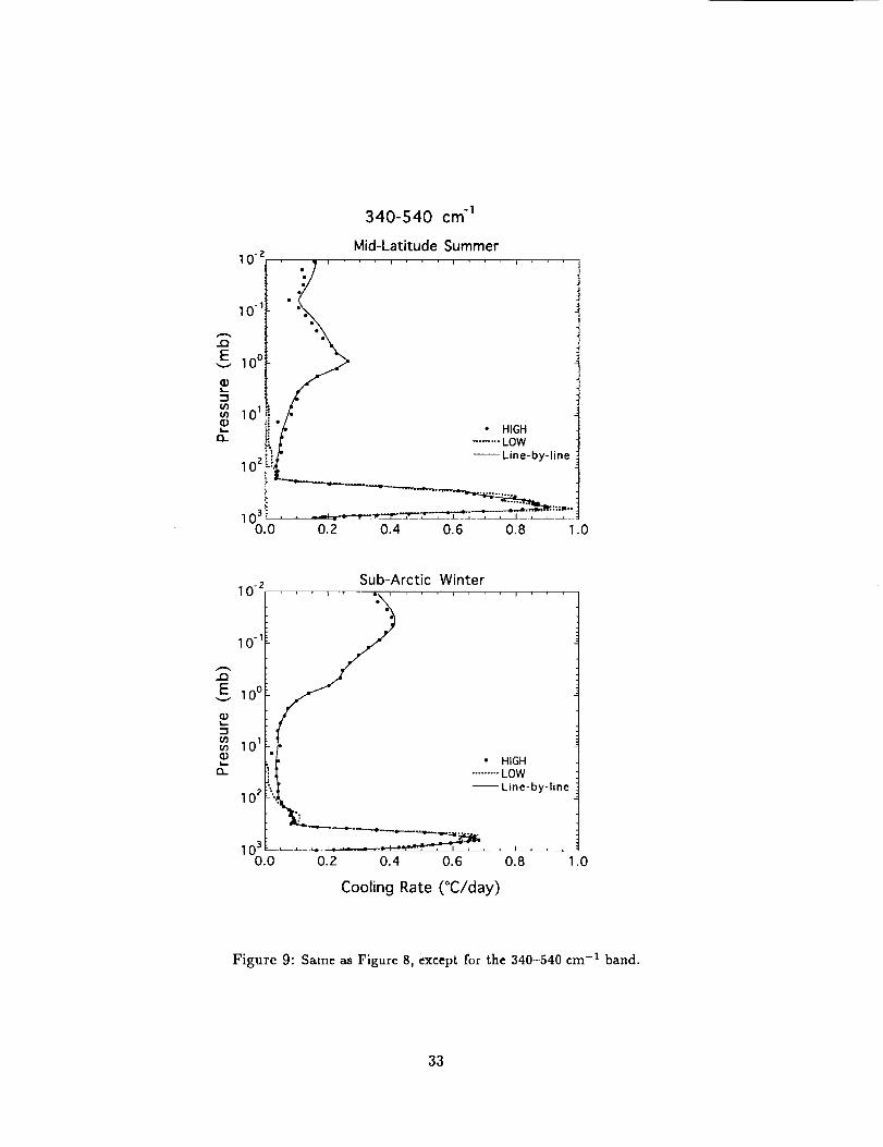
for the individual bands are shown in Figures 8 - 15 in Appendix A.
The cooling rate error for the total IR spectrum (Figure 5) is .._ 0.4 C day -1 in the mid-
dle atmosphere and .._ 0.2 C day -1 in the troposphere and lower stratosphere. For the
LOW option, the cooling rate is computed accurately in the lower atmosphere, at pressures
greater than _ 20 mb; above the 20 mb pressure level, the cooling rate computed using the
parameterization decreases rapidly to nearly zero. This is due to the pressure scaling of
the absorption, which greatly underestimates the cooling in low pressure regions. It can be
seen in the figures in the appendix that for the HIGH option, the cooling rate is computed
accurately not only for the total cooling but also for individual bands. The maximum error
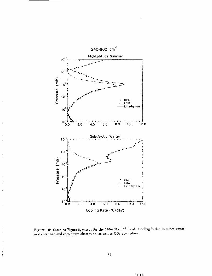
of .._ 0.4 C day -1 occurs in Band 3 (Figure 10) at pressures less than 1 mb. This error is
small when compared with the maximum cooling of 10-12 C day -1 due to CO2 at these
levels. Cooling rates in bands dominated by water vapor and ozone absorption are very
accurately computed, with errors of less than 0.2 C day -1.
25

-10-3000 cm
10 -z
lO'
E 10 0
*L
I/II/I
(D
e_
10 30.0
Mid-Latitude Summer
%°.°...,. • •
J ......... LOW
-- Line-by lone
2.0 4.0 6.0 8.0 10.0 12.0 14.0
Sub-Arctic Winter
lO'Z_,,.,..,,, _.,.,. , , . . , . , .
10.1 'i '\'",.....""-, "'--. i
E I 01
10 o- "'" . ....... •
._ "HIGH
Q- _ ........ LOW
--Line-by-line10 2
Io(;Lo2.-L .... , , , , , , , ___J , , , , , , ,• 2.0 4.0 6.0 8.0 10.0 12.0 14.0
Cooling Rate (°C/day)
Figure 5: Cooling rates computed using the line-by-line method (solid lines), the "LOW" option
(dashed lines), and the "HIGH" option (solid circles) for the total IR spectral region (0-3000 cm-1).
Cooling is due to water vapor molecular line and continuum absorption, as well as CO2 and O3absorption.
26
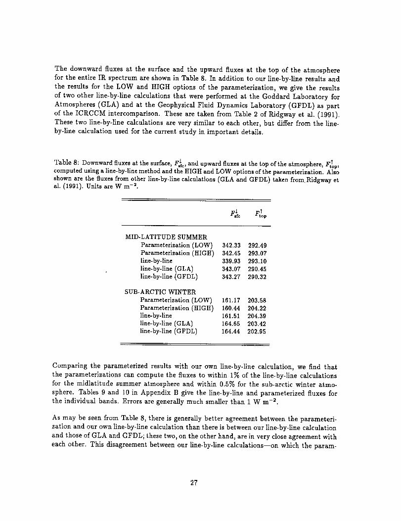
The downwardfluxesat the surface and the upward fluxes at the top of the atmosphere
for the entire IR spectrum are shown in Table 8. In addition to our line-by-line results and
the results for the LOW and HIGH options of the parameterization, we give the results
of two other line-by-line calculations that were performed at the Goddard Laboratory for
Atmospheres (GLA) and at the Geophysical Fluid Dynamics Laboratory (GFDL) as part
of the ICI_CCM intercomparison. These are taken from Table 2 of Pddgway et al. (1991).
These two line-by-line calculations are very similar to each other, but differ from the line-
by-line calculation used for the current study in important details.
Table 8: Downward fluxes at the surface, F_c , and upward fluxes at the top of the atmosphere, F_op,computed using a line-by-line method and the HIGH and LOW options of the parameterization. Also
shown are the fluxes from other line-by-line calculations (GLA and GFDL) taken from Ridgway etal. (1991). Units are W m -2.
MID-LATITUDE SUMMER
Parameterization (LOW) 342.33 292.49
Parameterization (HIGH) 342.45 293.07line-by-line 339.93 293.10
line-by-line (GLA) 343.07 290.45line-by-line (GFDL) 343.27 290.32
SUB-ARCTIC WINTER
Parameterization (LOW) 161.17 203.58
Parameterization (HIGH) 160.44 204.22line-by-line 161.51 204.39
line-by-line (GLA) 164.65 203.42line-by-line (GFDL) 164.44 202.95
Comparing the parameterized results with our own line-by-line calculation, we find that
the parameterizations can compute the fluxes to within 1% of the line-by-line calculations
for the midlatitude summer atmosphere and within 0.5% for the sub-arctic winter atmo-
sphere. Tables 9 and 10 in Appendix B give the line-by-line and parameterized fluxes for
the individual bands. Errors are generally much smaller than 1 W m -2.
As may be seen from Table 8, there is generally better agreement between the parameteri-
zation and our own line-by-line calculation than there is between our line-by-line calculation
and those of GLA and GFDL; these two, on the other hand, are in very close agreement with
each other. This disagreement between our line-by-line calculations--on which the param-
27

eterizations are based--and those used for ICR.CCM were somewhat disturbing. Since the
GLA calculation was done with essentially the same code as ours, but using the conditions
prescribed by the intercomparison, we could easily isolate the differences. Figure 6 shows
the differences for the upward and downward fluxes for the MLS and SAW atmospheres
between the GLA and our fine-by-line calculations. Differences in Bands 1, 5, and 7 are
small. Differences in bands 2, 3, 4, and 8 are of opposite sign at the top and bottom of the
atmosphere, with the upward flux at the top being larger in our calculations than in the
GLA calculations; this indicated some missing absorption in our calculations in these bands.
This effect is particularly large in Band 2. The difference in Band 6 is more perplexing.
These differences can be explained as follows:
The water vapor continuum absorption in the spectral region with strong molecular
line absorption is not adequately understood. We therefore do not include the water
vapor continuum absorption in the spectral region with wavenumber less than 540
cm -I, but the water vapor continuum absorption in the spectral region 400-540 cm -I
was included in the previous GLA and GFDL calculations. This discrepancy accounts
for most of the discrepancies in Band 2.
The absorption due to 03 in the 14/_m region, which was included in the previous GLAand GFDL calculations but not in the present study, contributes to the discrepancyin Band 3.
The minor CO2 bands located at 10.4/_m (in Band 4) and 9.4 #m (in Band 5) regions
were included in the previous GLA and GFDL calculations but not in the present
study. According to the line-by-line calculations of Kratz et al. (1993), each of the
two minor bands causes a reduction of 0.2-0.3 W m -2 in the top-of-the-atmosphereflux and an increase of 0.4-0.5 W m -2 in the surface flux.
The absorption due to C02 in the 4.3 #m band (in Band 8) was included in the
previous GLA and GFDL calculations but not in the present study. Most of the
discrepancies in Band 8 as shown in Figure 6 are due to the C02 absorption.
The current study uses the 1992 edition of the AFGL line parameters, while the
previous GLA and GFDL calculations used the 1986 edition. Integrated over 10
cm -1 spectral regions, the molecular line intensity of the 1992 edition is significantly
higher (with a maximun of 33%) than the 1986 edition in the 950-1500 cm -1 spectral
region (Bands 5 and 6). The large difference in the downward surface fluxes for the
midlatitude summer atmosphere is due to the use of different editions of the line
parameters.
These comparisons between the parameterized and line-by-line results and between the
various line-by-line calculations give some idea of the sources and magnitudes of the errors
that remain in the parameterization of the clear-sky IR radiation. As we can see from Table
28
_I II I

2
0
-2
-3
DOWNWARD FLUX AT SURFACE
2
I I I 1 I i 1 f
]
I 1 t I 1 I I I
1 2 3 4 5 6 7 8UPWARD FLUX AT TOP
I I l I I I [ I
-1
I I I I I __ __L__L_ . t
] 2 3 4 5 6 7 8BAND
Figure 6: Differences between the GLA and our line-by-line calculations for the downward flux at
the surface and the upward flux at the top of the atmosphere for the midlatitude summer (MLS)and sub-arctic winter (SAW) atmospheres. Positive values indicate our fluxes are larger than theGLA fluxes.
29
8, errorsdueto the broad-bandparameterizationof the line-by-line results are comparable
to the differences between the line-by-line results. The effects of neglecting the minor bands
of CO2 and O_ and of the uncertanty in modeling the water vapor continuum are significant.
We have also neglected the effects of minor infrared absorbers, most notably nitrous oxide
(NsO), methane (CH4), and the chlorofluorocarbons (CFCs). The total effect of neglecting
all the minor absorption bands is an underestimate of _ 5 W m -s in the downward flux
at the surface and an overestimate of _ 3 W m -2 in the upward flux at the top of the
atmosphere. We plan to include both the minor gases and the minor bands of the main
gases in future versions of the parameterization.
7 Summary
To achieve both requirements in accuracy and speed, various approaches are applied to
computing the transmission functions in various sections of the spectrum due to different
absorbers. There are two options for flux calculations, HIGH and LOW. For the HIGH
option, the k-distribution method with linear pressure-scaling is applied to those water vapor
spectral regions where absorption is not strong and where the contribution to the middle
atmospheric cooling is negligible. For the COs and 03 bands, as well as the water vapor
spectral regions with strong absorption, cooling in the middle atmosphere is significant,
and the transmittances are derived from pre-computed tables. For the LOW option, the
k-distribution method is used in all situations, except for the absorption due to ozone which
uses the table look-up method.
The HIGH option of the parameterization can compute accurately the cooling rate for the
middle and lower atmospheres from 0.01 mb to the surface. Errors are < 0.4 C day -1 in
cooling rates and < 1% in fluxes. The LOW option is computationally faster than the HIGH
option. It can achieve the same accuracy as the HIGH option except in the regions with
pressure < 20 mb. For the HIGH option of the parameterization, it takes 9.1 seconds to
compute the fluxes at 75 levels for 1000 soundings on a single processor of the CI_AY/C90
computer. For comparison, it takes 4.6 seconds to do the same computation with the LOW
option. Figure 7 shows each band's contribution to the total time. Bands 4, 5, 6, and 8
are the same for the two options. Bands 4 and 6 differ from Band 8 only in the presence of
continuum absorption, which evidently does not contribute significantly to the total cost.
In Bands 1, 2, and 7, the two options differ only in the treatment of water vapor line
absorption, which costs nearly four times as much when done with table look-up as when
done by the k-distribution method. With the HIGH option, Band 3 is the most costly due
to the use of a table look-up to compute the COs transmittances and to the separation into
three sub-bands used to compute the water vapor transmittances. For the LOW option,
Band 5 is the most costly due to the table look-up used to compute the 03 transmittances.
A LOW option without 03, which should be acceptable for tropospheric models, would be
considerably faster.
3O

2.5
r_ 2.0-
1.5-
_ 1.0
U
I
0.0i
C90TIMINGSWITH 75 LEVELSI ) I I i I I T
HIGH
LOW
1 2 3 4 5 6 7 8BAND
Figure 7: Execution times on a single Cray C90 processor.
In addition to the off-line testing described here, the parameterizations developed at God-
dard have been implemented and tested in long-term simulations in the climate and data
assimilation general circulation models at Goddard.
Acknowledgment: The authors are grateful to Dr. William Ridgway for providing them the
line-by-line calculated fluxes for comparisons with the parameterization and to Mr. Michael
Yan for assistance in testing the computer code. This work was supported by the Global
Atmospheric Modeling and Analysis Program, Office of Mission to Planet Earth, NASAHeadquarters.
31
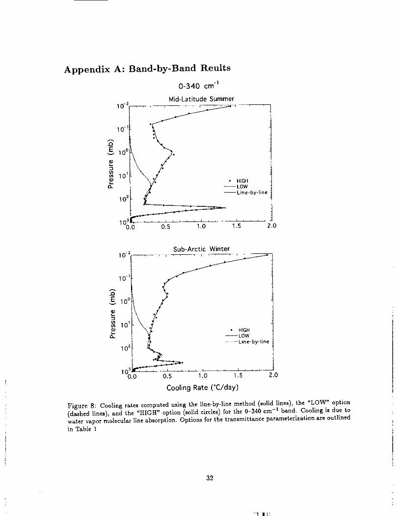
Appendix A: Band-by-Band Reults
-10-340 cm
lO
lO-
E i0c
q}o3
t_
101
102
1030.0
Mid-Latitude Summer
\. .
"" " HIGH
.] ........ LOW
,_ _ - Line-by-line
I _ _ , , .I0 J , , , ,_0.5 1 1.5 2.0
10 -z
10 -I
E 100
L
:3(D
101
¢L
I0 z
10 30.0
f
i..
"%*i •
• •
0.5 1.0
Sub-Arctic Winter
• HIGH......... LOW--Line-by-line
1.5 2.0
Cooling Rate (°C/day)
Figure 8: Cooling rates computed using the line-by-line method (solid lines), the "LOW" option(dashed lines), and the "HIGH" option (solid circles) for the 0-340 cm -1 band. Cooling is due towater vapor molecular line absorption. Options for the transmittance parameterization are outlinedin Table 1
32
-I340-540 cm
l('_,v "2 , , , ,
t"• °e
_ 10"11
..Q
10 0
_) 101
10 2
1030.0
Mid-Latitude Summer
• HIGH......... LOW
--Line-by-line
0.2 0.4 0.6 0.8 1.0
10 -z
10 -1
E 10 0
,0O'3
101
10 z
10 30.0
Sub-Arctic Winter
' • HIGH
i_ ......... LOW
,____ -- - Line-by-line
0.2 0.4 0.6 0.8 1.0
Cooling Rate (°C/day)
Figure 9: Same as Figure 8, except for the 340-540 cm -1 band.
33
-1540-800 cm
10 -z
10 1
IF 10o
(/1if)
0.
10 3 , , . I . , , I , , , I . , •
0.0 4.0 6.0 8.0 10.0 1Z.0
Mid-Latitude Summer• ' ' l ' ' ' I ' ' i , , , i , ' ' i , ,
%. •
IGH
....... LOW .- --Line-by-line
Z.O
Sub-Arctic Winter
10-I "',..
"%.. •
l_L-bv-linel0z
103 ...... l.......0.0 2.0 4.0 6.0 8.0 10.0 12.0
Cooling Rate (°C/day)
Figure 10: Same as Figure 8, except for the 540-800 cm -1 band. Cooling is due to water vapormolecular line and continuum absorption, as well as CO2 absorption.
34
:1 ! I

800-980 cm -1
Mid-Latitude Summer' I ' , , I
' ' I , , , I 1 , r_
200
.Q
E_-_ 400
• HIGH
L_ _. ......... LOW
_ 600 _ --Line-by-linex-
800 "_,_,__.""'.-i...
10001,, , I _ , I, ,_ I i , , 1 , __
O.0 0.2 0.4 0.6 0.8 1.0 .2
0Sub-Arctic Winter
' ' ' ' I .... I ' ' , . I ' ' ' ' I '
200
E 4oo. • HIGH
o "x.._ -........LOW_... --Line-by-line
600 _...
" "".L°"'-e.
.M"
0.00 0.01 0.02 0.03 0.04 0.05
Cooling Rate (°C/day)
Figure 11: Same as Figure 8, except for the 800-980 cm -1 bandl Cooling is due to water vapormolecular line and continuum absorption. Note that the HIGH and LOW options are identical inthis band.
35

-1980-1100 cm
Mid-Latitude Summer10 .2 .... ,... , .... , .... ,., , , ,
.-. 10-1 _''' '
lo'L- / • HIGH
t_ ._/ ........ LOW
10 z _ . ----Line-by-line
10 3 , _ ,., .... _ .... _ __h._-1.0 -0.5 O.0 0.5 1.0 1.5 2.0 2.5 3.0
Sub-Arctic Winter10 z .... , .... ,, ,., .... , ......... , .... , ....
i0_
JO
_E I0Oi
I01LIGH
_- _ ........ LOW
10z _ t . --.Line-by-line
u_' -O.5 0.0 0.5 1.O 1.5 2.0 Z.5 3.01 0
Cooling Rate (°C/day)
Figure 12: Same as Figure 8, except for the 980-1100 cm -I band. Cooling is due to water vapor
molecular line and continuum absorption, as well as 03 absorption.
36
_11 F
-I1 I00-I 380 cm
Mid-Latitude Summer
200 -
• HIGH\',, ........ LOW
"_ --Line-by-line600
800
_°°8/'"0:_'" 0.2 0.3 0._ 0.5 0.6
200
Sub-Arctic WinterI I I I
_O
E 400-"_-_.... • HIGH
_ ...... "........ LOW
_ ...... . --Line-by-line600 _ ..........
800_..._
1000 _ ........ _ , , ,0.00 0.02 0.04 0.06 0.08 0.10
Cooling Rate (°C/day)
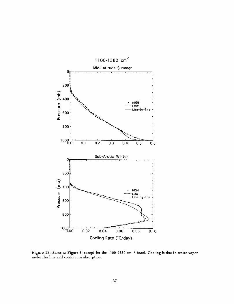
Figure 13: Same as Figure 8, except for the 1100-1380 cm -1 band. Cooling is due to water vapor
molecular line and continuum absorption.
37
1380-1900 cm -1
lO -z
10 "I
IE 100
{/1(/1I..
t_
101
10z
Mid-Latitude Summer
!
..iG.t .........LOW
"L:,._ - - - Line-by-line
-0.1 0.0 0.1 0.2 0.3 0.4
Sub-Arctic Winter10 "z .... f ....... ,,,,
O iE 100
o
(/1o
10_
10 z
10 3 .... , .... _',
-0.2 -0.1 0.0 0.1
° HIGH......... LOW--Line-by-line
.... I , , , , l i _ L i
0.2 0.3 ).4
Cooling Rate (°C/day)
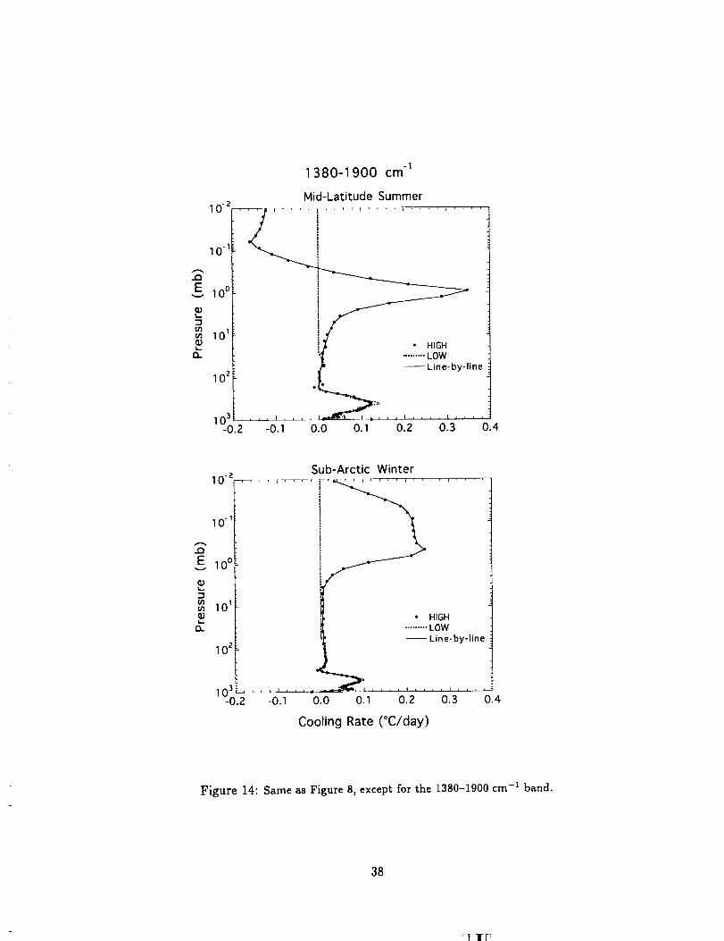
Figure 14: Same as Figure 8, except for the 1380-1900 cm -1 band.
38
-I1900-3000 cm
Mid-Latitude Summer
200
E_._ 400
_, • HIGH,o _ .........LOW:3 "..'_.. _ Line-by-line
g- ""i,.
800 _'__
,ooo" "_().00 0.01 0.02 0.03 0.04 0.05 0.06
Sub-Arctic Winter
200
..Q
E 400 ,
_ • HIGH"_.."_ ......... LOW
800 ..... ".........
"'_6"'°.-i
.... 4"""
• ..........e'" "" ...... e' ......
00 0.002 0.004 0.006 0.008 0.010
Cooling Rate (°e/day)
Figure 15: Same as Figure 8, except for the 1900-3000 cm -1 band.
3g
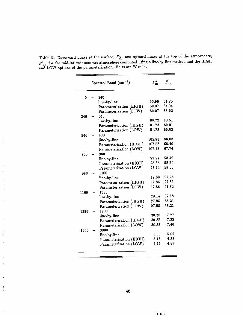
Table 9: Downward fluxes at the surface, F_¢, and upward fluxes at the top of the atmosphere,
F_op, for the mid-latitude summer atmosphere computed using a line-by-line method and the HIGHand LOW options of the parameterlzation. Units are W m -_.
Spectral Band (cm -1) F,_c F,Top
340
540
800
980
1100
1380
1900
340
line-by-line 50.96 34.25Parameterization (HIGH) 50.97 34.04
Parameterization (LOW) 50.97 33.92
540line-by-line 80.72 60.51Parameterization (HIGH) 81.23 60.01
parameterization (LOW) 81.28 60.03
800
line-by-line 105.98 68.03Parameterization (HIGH) 107.58 68.40
Parameterization (LOW) 107.43 67.74
980
line-by-line 27.97 58.49Parameterization (HIGH) 28.35 58.50parameterization (LOW) 28.34 58.50
1100
line-by-line 12.80 22.28
Parameterization (HIGH) 12.86 21.81
Parameterization (LOW) 12.86 21.82
1380
line-by-line 28.14 37.18Parameterization (HIGH) 27.95 38.21
Parameterization (LOW) 27.95 38.21
1900
line-by-line 30.30 7.27parameterization (HIGH) 30.35 7.22
parameterization (LOW) 30.33 7.40
3000line-by-line 3.06 5.09
Parameterization (HIGH) 3.16 4.88Parameterization (LOW) 3.16 4.88
40
_1 1]_

Table 10: Same as Table 9, except for the sub-arctic winter atmosphere.
Spectral Band (cm -1) F_¢ F]op
0 - 340
line-by-line 40.39 32.10
Parameterization (HIGH) 40.40 31.93
Parameterization (LOW) 40.40 31.82340 - 540
line-by-line 47.35 52.01
Parameterization (HIGH) 47.30 51.74
Parameterization (LOW) 48.09 51.78540 - 800
line-by-line 53.17 51.38
Parameterization (HIGH) 51.84 51.65
Parameterization (LOW) 51.90 51.06800 - 980
line-by-llne 1.45 32.85
Parameterization (HIGH) 1.63 32.86
Parameterization (LOW) 1.63 32.86980 - 1100
line-by-line 3.14 10.99
Parameterization (HIGH) 3.23 10.87
Parameterization (LOW) 3.22 10.871100 - 1380
line-by-line 5.49 18.80
Parameterization (HIGH) 5.49 18.98
Parameterization (LOW) 5.50 18.981380 - 1900
line-by-line 10.11 4.90
Parameterization (HIGH) 10.13 4.87
Parameterization (LOW) 10.02 4.901900 - 3000
line-by-line 0.41 1.36
Parameterization (HIGH) 0.42 1.32
Parameterization (LOW) 0.43 1.32
41

Appendix B: The Code
The following is a listing of the FORTRAN implementation of the parameterization. This
code follows the "plug-compatible" rules of Kalnay et al. (1988), which should make it easy
to use in climate models. The parameterization is accessed by calling subroutine IRKAD.
All information needed by this subroutine is passed through the argument list and all
results are returned through the argument list. Its arguments are described in detail in the
comments at the top of the code.
The inputs to the routine are a two-dimensional (M by N) array of soundings, with each
sounding consisting of NP layers. The temperature, the specific humidity, the ozone mixing
ratio, and the cloud fraction and optical thickness are specified at the NP layers, while
the pressure is specified at the NP-1 interfaces and at the lower and upper boundaries.
The surface temperature is also required. The CO2 concentration is assumed constant
throughout the atmosphere.
Although the routine processes M by N soundings, all input and output arrays are dimen-
sioned M by NDIM, where NDIM > N. This is done so that a large array can be stripmined
over the outer dimension without the need to make copies. Such stripmining is useful in
parallel applications and when trying to minimize storage, since the scratch space required
by the routine is proportional to M*N.
The outputs of the routine are the net downward all-sky and clear-sky fluxes and the rate of
change of the all-sky flux with respect to surface temperature. The routine also returns the
upward flux at the surface, i.e., the approximate form of aT_ used in the parameterization.
This allows the calling program to maintain energetic consistency by using this value in the
surface energy budget.
42
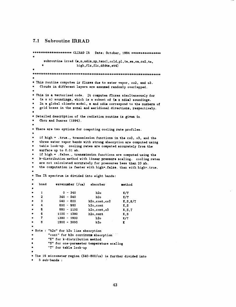
7.1 Subroutine IRRAD
* The IR spectrum is divided into eight bands:
********************* CLIRAD IR Date: October, 1994 ****************
,
subroutine irrad (m,n,ndim,np,taucl,ccld,pl,ta,wa,oa,co2,ts,
* high,flx,flc,dfdts_st4)
* This routine computes ir fluxes due to water vapor, co2, and 03.
* Clouds in different layers are assumed randomly overlapped.
* This is a vectorized code. It computes fluxes simultaneously for
* (m x n) soundings, which is a subset of (m x ndim) soundings.
* In a global climate model, m and ndim correspond to the numbers of
* grid boxes in the zonal and meridional directions, respectively.
* Detailed description of the radiation routine is given in
* Chou and Suarsz (1994).
* There are tgo options for computing cooling rate profiles.
if high = .true., transmission functions in the co2, o3, and the
three water vapor bands with strong absorption are computed using
table look-up, cooling rates are computed accurately from the
surface up to 0.01 mb.
if high = .false., transmission functions are computed using the
k-distribution method gith linear pressure scaling, cooling rates
are not calculated accurately for pressures less than 20 mb.
the computation is faster with high=.false, than with high=.true.
wavenumber (/cm) absorber method
0 - 340 h2o K/T
340 - 840 h2o K/T
840 - 800 h2o,cont,co2 K,S,K/T
800 - 980 h2o,cont K,S
980 - 1100 h2o,cont,o3 K,S,T
1100 - 1380 h2o,cont K,S
1380 - 1900 h2o K/T
1900 - 3000 h2o g
: "h2o" for h2o line absorption
"cont" for h2o continuum absorption
"K" for k-distribution method
"S" for one-parameter temperature scaling
"T" for table look-up
* bnad
* I
* 2
* 3
* 4
* 5
* 6
* 7
* 8
* Note
* The 15 micrometer region (540-800/cm) is further divided into
* 3 sub-bands :
43

* subbnad _avenu.mbar (/oR)
* I 540 - 620
* 2 620 - 720
* 3 720 - 800
* .... Input parameters
* cJ , c2, c3: for co2 (band 3)
* ol , 02, 03: for 03 (band 5)
* h11,h12,h13: for h2o (band 1)
* h21,h22,h23: for h2o (band 2)
* h71,h72,h73: for h2o (band 7)
* .... output parameters
* net downward flux, all-sky
* Notes:
number of soundings in zonal direction (m)
number of soundings in meridional direction (n)
maximum nu_ber o3 soundings in
meridional direction (ndim)
number of atmospheric layers (up)
cloud optical thickness (taucl)
cloud cover (ccld)
level pressure (pl)
layer temperature (ta)
layer specific humidity (.a)
layer ozone mixing ratio by mass (oa)
surface temperature (ts)
co2 mixing ratio by voltmn (co2)
high
units size
n/d 1
n/d 1
n/d I
n/d I
n/d m*ndim*np
fraction m*ndim*np
mb m*ndim*(np+l)
k m*ndim*np
g/g m*ndim*np
g/g m*ndim*np
k m*ndim
ppmv 1
i
pre-computed tables used in table look-up for transmittance calculations:
w/m**2 m*ndim*(np+l)
w/m**2 m*ndim*(np+1)
w/m**2/k m*ndim*(np+1)
"/m**2 m*ndim
(fix)
net downward flux, clear-sky (flc)
sensitivity of net downward flux
to surface temperature (dfdts)
emission by the surface (st4)
* (1) Water vapor continuum absorption is included in 840-1380 /cm.
* (2) Scattering by clouds is not included.
* (3) Clouds are assumed "gray" bodies.
* (4) The diffuse cloud transmission is computed to be exp(-1.66*tauci).
* (5) I_ there are no clouds, flx=_Ic.
* (6) plevel(1) is the pressure at the top of the mOdei_atmosphere, and
* plevel(np+1) is the surface pressure. ".....
, (7) Downward flux is positive, and upward flux is negative.
* (8) dfdts is always negative because upwar. _ flux =is defined as negative.
* (9) For questions and coding errors, please contact with Ming-DahChou,
* Code 913, NASA/Goddard Space Flight Center, Greenbelt, MD 20771.
44
rl !!i
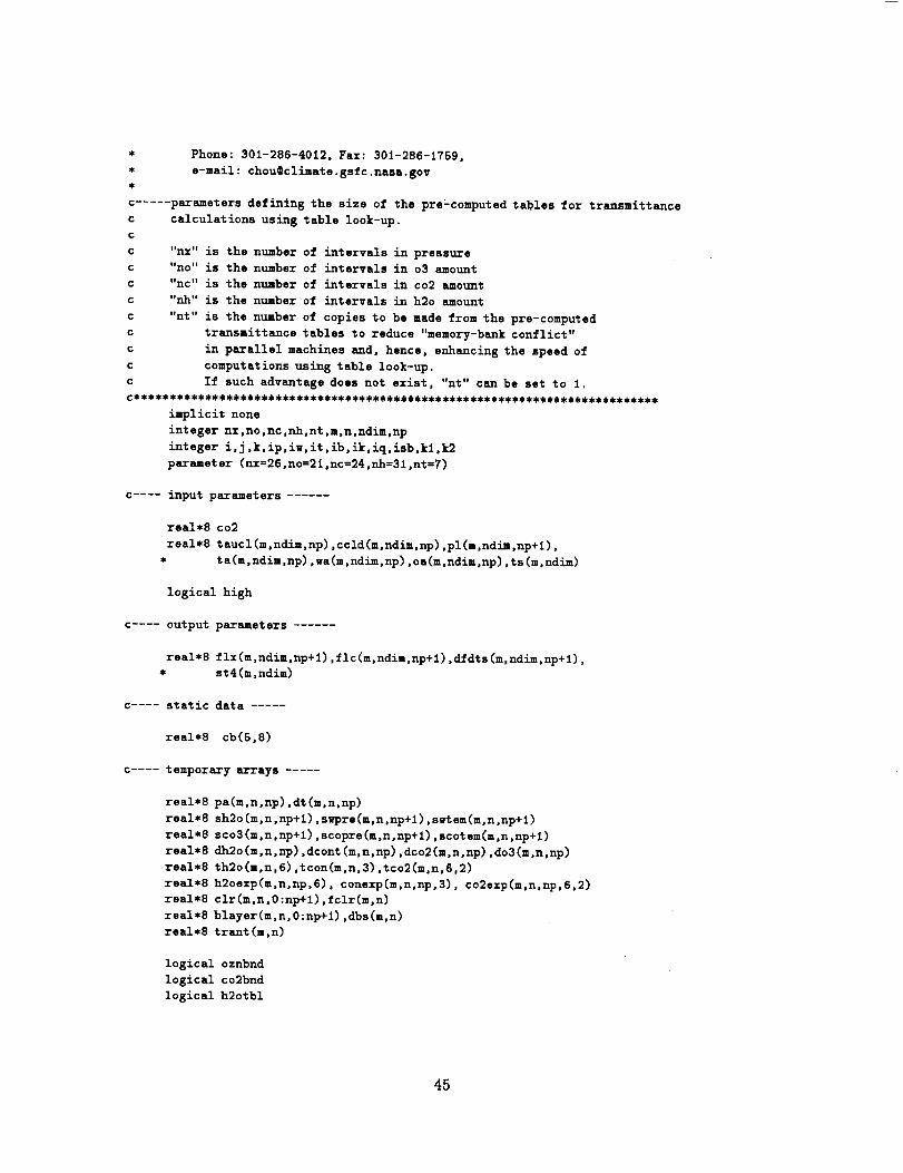
* Phone: 301-286-4012, Fax: 301-286-1759,
* e-mail: [email protected]
c ..... parameters defining the size of the preLcomputed tables for transmittance
calculations using table look-up.C
C
c "nx" is the number of intervals in pressure
c "no" is the number of intervals in 03 amount
c "nc" is the number of intervals in co2 amount
c "nh" is the number of intervals in h2o amount
c "nt" is the number of copies to be made from the pre-computed
c transmittance tables to reduce "memory-bank conflict"
c in parallel machines and, hence, enhancin 8 the speed of
c computations using table look-up.
c If such advantage does not exist, "nt" can be set to I.
implicit none
integer nx,no,nc,nh,nt,m,n,ndim,np
integer i,j,k,ip,iw,it,ib,ik,iq,ieb,kl,k2
parameter (nx=26,no=21,nc=24,nh=S1,nt=7)
c .... input parameters ......
real*8
real*8
co2
taucl(m,ndim,np),ccld(m,ndim,np),pl(m,ndim,np+l),
ta(m,ndim,np),ea(m,ndim,np),oa(m,ndim,np),ts(m,ndim)
logical high
c .... output
real*8
parameters ......
_ix(m,ndim,np+1),flc(m,ndim,np+l),dfdts(a,ndim,np+1),
st4(m,ndim)
c .... static data .....
real*8 cb(5,8)
C .... temporary arrays .....
real*8
real*8
real*8
real*8
real*8
real*8
real*8
real*8
real*8
pa(m,n,np),dt(m,n,np)
sh2o(m,n,np+1),swpre(m,n.np+1),swtem(m,n,np+1)
sco3(m,n,np+l),scopre(m,n,np+1),scotem(m,n,np+l)
dh2o(m,n,np),dcont(m,n,np),dco2(m,n,np),do3(m,n,np)
th2o(m,n,6),tcon(m,n,3),tco2(m,n,6,2)
h2oexp(m,n,np,6), conexp(m,n,np,3), co2exp(m,n,np,6,2)
clr(m,n,O:np+l),fclr(m,n)
blayer(m,n,O:np+l),dbs(m,n)
trant(m,n)
logical oznbnd
logical co2bnd
logical h2otbl
45

logical conbnd
real*8 cl (nx,nc,nt),c2 (nx,nc,nt),c3 (nx,nc,nt)
real*8 ol (nx,no,nt),o2 (nx,no,nt),o3 (nx,no,nt)
real*8 hll(nx,nh,nt),h12(nx,nh,nt),h13(r_,nh,nt)
real*8 h21(nx,nh,nt),h22(nx,nh,nt),h23(nx,nh,nt)
real*8 h71(nx,nh,nt) 0h72(nx,nh,nt),h73(nx,nh,nt)
real*8 dp,xx,trantc
c ..... the following coefficients (table 2 of chou and susrez, 1995) are for
c computing spectrally integtrated planck fluxes of the 8 bands using
eq, (22)
data cb/
I -2.6844e-1,-8.8994e-2
2 3.7315s+l,-7.4758e-I
3 3.7187e+1,-3.9085e-1
4 -4.1928e+1, 1.0027e+0
5 -4.9163e+1, 9.8457e-1
6 -1.0345e+20 1.8636s+0
7 -6.9233e+O,-1.5878e-1
8 1.1483e+2,-2.2376e+O
1.5676e-3
4.6151e-3
-6.1072e-4
-8.5789e-3
-7.0968e-3
-1.1753e-2
3.9160e-3
1.6394e-2
-2.9349e-6, 2.2233e-9,
-6.3260e-6, 3.5647e-9,
1.4534e-5,-1.6863e-8,
2.9199e-5,-2.5654e-8,
2.0478e-5,-1.SS14e-8,
2.7864e-5,-1.1998e-8,
-2.4496e-5, 4.9301e-8,
-5.3672e-5, 6.6456e-8/
c ..... copy tables to enhance the speed of co2 (band 3), 03 (bandS),
c and h2o (bands 1, 2, and 7 only) transmission calculations
c using table look-up.
logical first
data first /.true./
include "h2o.tran3"
include "co2.tran3"
include "o3.tran3"
save cl,c2,c3,ol,o2,o3
save h11,h12,h13,h21,h22,h23,h71,h72,h73
if (first) then
c ..... tables co2 and h2o are only used with 'high' option
if (high) then
do i.=l,nh
do ip=l,nx
hll(ip,iw,l)=l.O-hll(ip,iw01)
h21(ip,iw,1)=l.0-h21(ip,iw,1)
h71(ip,iw,1)=l.0-h71(ip,iw,l)
enddo
enddo
46
_I 1i:
do iw=Itnc
do ip=l,nx
c1(ip,iw.1)=l.0-cl(ip,iw,l)
enddo
enddo
c ..... tables are replicated to avoid memory bank conflicts
do it=2,nt
do iw=l,nc
do ip=l,nx
cl (ip,iw,it)= c1(ip,iw,1)
c2 (ip,iw,it)= c2(ip,iw,1)
c3 (ip,iw_it)= c3(ip,iw,1)
enddo
enddo
do iw=l.nh
do ip=l,nx
bll(ip,iw,it)=hli(ip.i,,l)
h12(ip.iw,it)=h12(ip.iw,1)
hl3(ip,iw,it)=hl3(ip,iw,1)
b21(ip,iw_it)=b21(ip,iw_l)
h22(ipoiw,it)=h22(ip,iw,1)
h23(ip,iw,it)=h23(ip.iw.1)
h71(ip,iw,it)=hTl(ip,iw,1)
h72(ip,iw,it)=h72(ip.iw,l)
hT3(ip,iw,it)=h73(ip,iw,l)
enddo
enddo
enddo
endif
c ..... always use table look-up for ozone transmittance
do iw=1.no
do ip=l,nx
ol(ip,iw.l)=l.O-ol(ip.iw.1)
enddo
enddo
do it=Rsnt
do iw=l,no
do ip=l.nx
ol (ip.iw,it)= ol(ip.iw,1)
02 (ip,iw,it)= o2(ip.iw,1)
03 (ip.iw.it)= o3(ip.iw.1)
enddo
enddo
enddo
first=.false.
47
endif
c ..... compute layer pressure (pa) and layer temperature minus 260K (dr)
do k=1,np
do j=1,n
do i=l,m
pa(i,j,k)=O.5*(pl(i,j,k)+pl(i,j,k+1))
dt(i,j,k)=ta(i,j,k)-250.O
enddo
enddo
enddo
c ..... compute layer absorber amount
dh2o : water vapor amount (g/cm**2)
dcont: scaled water vapor amount for continuum absorption (8/cm*.2)
dco2 : co2 amount (cm-atm)stp
dos : o3 amount (cm-atm)stp
the factor 1.02 is equal to 1000/980
factors 789 and 476 are for unit conversion
the factor 0.001618 is equal to 1.02/(.622.1013.25)
the factor 6.081 is equal to 1800/296
do k=_ ,np
do j=1,n
do i=l,m
dp = pl(i,j,k+l)-pl(i,j,k)
dh2o (i,j,k) = 1.02*wa(i,j,k)*dp+1.e-lO
dco2 (i,j,k) = 789.*co2*dp+1.e-10
dos (i,j,k) = 476.0*oa(i,j,k)edp+l.e-lO
c ..... compute scaled water vapor amount for h2o continuum absorption
c following eq. (43).
xx=pa(i,j,k)*O.OO1618*wa(i,j,k)*wa(i,j,k)*dp
dcont(i,j0k) = xx*exp(18OO./ta(i,j,k)-6.081)+J.e-JO
c ..... compute effective cloud-free fraction, clr, for each layer.
c the cloud diffuse transmittance is approximated by using a
c diffusivity factor of 1.66.
clr(i,j,k)=1.0-(ccld(i,j,k)*(1.-sxp(-1.66*taucl(i,j,k))))
enddo
enddo
enddo
c ..... compute column-integrated h2o amoumt, h2o-weighted pressure
c and temperature, it follows eqs. (37) and (38).
if (high) then
48

call oolumn(m,n,np,pa,dt,dh2o,sh2o,swpre,swtem)
endif
c ..... the surface (with an index np+l) is treated as a layer filled with
c black clouds.
do j=i,n
do i=i,m
clr(i,j,O) = i.O
clr(i,j,np+l) = 0.0
st4(i,j) = 0.0
enddo
enddo
c ..... initialize fluxes
do k=l,np+1
do j=i,n
do i=i,m
flx(i,j,k) = 0.0
flc(i,j.k) = 0.0
dfdts(i,j,k)= 0.0
enddo
enddo
enddo
c..... integration over spectral bands
do I000 ib=i,8
c ..... if h2otbl, compute h2o (line) transmittance using table look-up.
c if conbnd, compute h2o (continuum) transmittance in bands 3, 4, 5 and 6.
c if co2bnd, compute co2 transmittance in band 3.
c if oznbnd, compute 03 transmittance in band 5.
h2otbl=high.and.(ib.eq.l.or.ib.eq.2.or.ib.eq.7)
conbnd=ib.ge.3.and.ib.le.6
co2bnd=ib.eq.3
oznbnd=ib.eq.5
c ..... blayer is the spectrally integrated planck flux of the mean layer
c temperature derived from eq. (22)
do k=l,np
do j=l,n
do i=l,m
blayer(i,j,k)=ta(i.j,k)*(ta(i,j,k)*(ta(i,j,k)
$(ta(i,j,k)*cb(5,ib)+ob(4,ib))+cb(3,ib))
+cb(2,ib))+cb(10ib)
enddo
enddo
49
enddo
c ..... the earth's surface, with an index "np+1", is treated as a layer
do j=l.n
do i=l,m
blayer(i,j,O) = 0.0
blayer(i,j,np+l)=ts(i,j)*(ts(i,j)*(ts(i,j)
, *(ts(i,j)*cb(5,ib)+cb(4,ib))+cb(3,ib))
. +cb(2,ib))+cb(1,ib)
c ..... dbs is the derivative of the surface planck flux with respect to
c surface temperature (eq. 59).
dbs(i,j)=ts(i,j)*(ts(i,j)*(ts(i,j)
, .4..cb(5,ib)+3.*cb(4,ib))+2.*cb(3,ib))+cb(2,ib)
enddo
enddo
c ..... compute column-integrated absorber amoumt, absorber-weighted
c pressure and temperature for co2 (band 3) and 03 (band 5).
c it folloss eqs. (37) and (38).
c ..... this is in the band loop to save storage
if( high .and. co2bnd) then
call column(m,n,np,pa,dt,dco2,sco3,scopre,scotem)
endif
if(oznbnd) then
call column(m,n,np,paodt,do3,sco3,scoprs,scotem)
endif
c ..... compute the exponential terms (eq. 32) at each layer for
c water vapor line absorption when k-distribution is used
if( .not. h2otbl) then
call h2oexps(ib,m,n,np,dh2o,pa,dt,h2oexP)
endif
c..... compute the exponential terms (eq. 46) at each layer for
c water vapor continuum absorption
if(conbnd) then
call conexps(ib,m,n,np.dcont,conexP)
5O
"'! 11_
endif
c ..... compute the exponential terms (eq. 32) at each layer for
c c02 absorption
if( .not.high .and. co2bnd) then
call co2exps(m,n,np0dco2,pa,dt,co2exp)
endif
c ..... compute transmittances for regions between levels kl and k2
c and update the fluxes at the two levels.
do 2000 kl=l,np
c ..... initialize fclr, th2o, tcon, and tco2
do j=l,n
do i=l,m
fclr(i,j)=l.0
enddo
enddo
c ..... for h2o line absorption
if(.not, h2otbl) then
do ik=l,6
do j=1,n
do i=l,m
th2o(i,j,ik)=l.O
enddo
enddo
enddo
endif
c ..... for h2o continuum absorption
if (conbnd) then
do iq=1,3
do j=l,n
do i=i,a
tcon(i,j,iq)=1.0
enddo
enddo
enddo
endif
c ..... for co2 absorption when using k-distribution method.
c band 3 is divided into 3 sub-bands, but sub-bands 3a and 3c
¢ are combined in computing the co2 transmittance.
51
if (.not. high .and. co2bnd) then
do isb=l,2
do ik=l,6
do j=1 ,n
do i=1,m
tco2 (i, j, ik, isb) =I. 0
enddo
enddo
enddo
enddo
endif
c ..... loop over the bottom level of the region (k2)
do 3000 k2=kl+1,np+1
do j=1,ndo i=l,m
trant (i, j)=l.0
enddo
enddo
if(h2otbl) then
c..... compute water vapor transmittance using table look-up
if (ib.eq.l) then
call tablup(kl.k2.m.n.np.nx.nh.nt.sh2o.swpre.swtem.
* -8.0,-2.0,O.3,O.2,h_1,h12,h13,trant)
endif
if (ib.sq.2) then
call tablup(kl,k2,m,n,np,nx,nh,nt,sh2o,s,pre,swtem,
, -8.0_-2.0,O.3,0.2,h21,h22,h23,trant)
endif
if (ib.eq.7) then
call tablup(kl.k2.m.n.np.nx.nh.nt.sh2o.swpre.s,tsm.
-8.0,-2.0,O.3,0.2,hTl,h72,h73,trant)
endif
else
c ..... compute water vapor transmittance using k-distribution.
call wvkdis(ib,m,n,np,k2-l,h2oexp,conexp,th2o,tcon,trant)
endif
52
if(co2bnd) then
if( high ) then
c ..... compute co2 transmittance using table look-up method
call tablup(kl,k2,m,n,np,nx,nc,nt,sco3,scopre,scotem,
-4.0,-2.0,O.3,0.2,cl,c2,c3,trant)
else
c ..... compute co2 transmittance using k-distribution method
call co2kdis(m,n,np,k2-1,co2exp,tco2,trant)
endif
endif
c ..... compute 03 transmittance using table look-up
if (oznbnd) then
call tablup(kl,k2,m,n,np,nx,no,nt,sco3,scopre,scotem,
* -6.0,-2.0,O.3,0.2,ol,o2,o3,trant)
endif
c ..... fclr is the clear line-of-sight between levels kl and k2.
c in computing fclr, clouds are assumed randomly overlapped
c using eq. (10).
do j=i,n
do i=i,m
fclr(i,j) = fclr(i,j)*clr(i,j,k2-1)
enddo
enddo
c..... compute upward and downward fluxes
c ..... add "boundary" terms to the net downward flux.
c these are the first terms on the right-hand-side of
c eqs. (56a) and (56b).
c downward fluxes are positive.
if (k2 .eq. kl+l) then
do j=l,n
do i=l,m
flc(i,j,kl)=flc(i,j,kl)-blayer(i,j,kl)
flc(i,j,k2)=flc(i,j,k2)+blayer(i,j,kl)
53

flx(i,j,kl)=flx(i,j.kl)-blayer(i,j,kl)
flx(i.j,k2)=flx(i,j,k2)+blayer(i,j,kl)
enddo
enddo
endif
c ..... add flux components involving the four layers above and below
c the levels kl and k2. it follows eqs. (56a) and (56b).
do j=l,n
do i=l,m
xx=trant(i,j)*(blayer(i,j,k2-1)-blayer(i,j,k2))
flc(i,j,kl) =flc(i,j,kl)+xx
flx(i,j,kl) =flx(i,j,kl)+xx*fclr(i,j)
xx=trant(i,j)*(blayer(i,j,k1-1)-blayer(i,j,kl))
flc(i,j,k2) =flc(i,j,k2)+xx
flx(i,j,k2) =flx(i,j,k2)+xx_fclr(i,j)
snddo
enddo
3000 continue
c ..... compute the partial derivative of fluxes with respect to
c surface temperature (eq. 59).
do j=l,n
do i=l,m
dfdts(i,j,kl) =dfdts(i,j,kl)-dbs(i,j)*trant(i.j)*fclr(i,j)
enddo
enddo
2000 continue
c..... add contribution from the surface to the flux terms at the surface.
do j=l,n
do i=1.m
dfdts(i,j,np+1) =dfdts(i,j,np+l)-dbs(i,j)
enddo
enddo
do j=l,n
do i=l,m
flx(i,j.np+l)=flx(i,j,np+l)-blayer(i,j.np+l)
flc(i,j,np+l)=flc(i,j,np+1)-blaysr(i,j,np+l)
st4(i,j)=st4(i,j)-blayer(i,j,np+1)
enddo
enddo
54

1000 continue
_etu._n
end
r55
7.2 Subroutine COLUMN
***************************************************************************
subroutine column (m,n,np,pa,dt,sabs0,sabs,sl::_e,stem)
O
c ..... compute coltmn-integrated (from top of _he model atmosphere)
c absorber amount (sabs), absorber-weighted pressure (spre) and
c temperature (stem).
c computations of spre and stem follows
c eqs. (37) and (38) of Chou and Suarez (1994).
C
c--- input parameters
c number of so_mdings in zonal direction (m)
c number of soundings in meridional direction (n)
c number of atmospheric layers (np)
c layer pressure (pa)
c layer temperature minus 250K (dr)
c layer absorber amount (sabsO)
¢
c--- output parameters
c coluEn-integrated absorber amount (sabs)
c column absorber-weiahted pressure (apre)
c column absorber-weighted temperature (stem)
C
c--- units of pa and dt are mb and k, respectively.
c units of sabs are g/cm*e2 for water vapor and (cm-atm)stp for co2 and o3
implicit none
integer m,n,np,i,j ,k
c .... input parameters .....
real*8 pa(m.n.np).dt(m.n.np).sabsO(m,n.np)
c .... output parameters .....
real*8 sabs(m,n,np+l),spre(m,n,np+l),stem(m,n,np+l)
**********************************************************************
do j=l,n
do i=1,m
sabs(i,j,1)ffiO.O
spre(i,j,l)=O.O
stem(i,j,1)=O.O
enddo
enddo
do k=l,np
do jfl,n
do i=l,m
sabs(i,j,k+l)fsabs(i,j,k)+sabsO(i,j,k)
56
7 | F]

spre(i,j,k+l)=spre(i,j,k)+pa(i,j,k)*sabsO(i,j,k)
stem(i,j,k+l)=stem(i,j,k)+dt(i,j,k)*sabsO(i,j,k)
enddo
enddo
enddo
return
end
57

7.3 Subroutine TABLUP
***********************************************************************
subroutine t ahlup (kl ,k2 ,m, n,np ,nx, nh,nt ,sabs ,spre, stem,wl ,pl,
* dwe, dpe, coef I, coal2, coef 3, tran)
***********************************************************************
c compute water vapor, co2, and 03 transmittances between levels kl and k2
c using table look-up for m x n soundings.
C
c Calculations follow Eq. (40) of Chou and $uarez (1994)
C
c .... input .....................
c indices for pressure levels (kl and k2)
c number of grid intervals in zonal direction (m)
c number of grid intervals in meridional direction (n)
c number of atmospheric layers (np)
c number of pressure intervals in the table (nx)
c number of absorber amount intervals in the table (nh)
c number of tables copied (nt)
c column-intesrated absorber amount (sabs)
c column absorber amount-weishted pressure (spre)
c column absorber amount-weighted temperature (stem)
c first value of absorber amount (Io810) in the table (wl)
c first value of pressure (loglO) in the table (pl)
c size of the interval of absorber amount (loglO) in the table (dwe)
c size of the interval of pressure (loglO) in the table (dpe)
C pre-computed coefficients (coefl, coal2, and coal3)
C
c .... updated .....................
c transmittance (tran)
C
c Note:
c (I) units of sabs are g/cm**2 for water vapor and (cm-atm)stp for co2
and 03.
c (2) units of spre and stem are, respectively, mb and K.
c (3) there are nt identical copies of the tables (coefl, coal2, and
c coal3), the prupose of using the multiple copies of tables is
c to increase the speed in parallel (vectorized) computations.
C if such advantage does not exist, nt can be set to I.
C
c .... input parameters .....
real*8 wl,pl,dwe,dpe
real*8 sabs(m,n,np+l),spre(m,n,np+l),stea(m,n,np+l)
real*8 coefl(nx,nh,nt),coef2(nx,n_h,nt),coef3(nx,r_,nt)
c .... update parameter .....
58

real*8 tran(m,n)
c .... temporary variables .....
real*8 xl,x2,x3,we,pe,fw,fp,fm,pa,pb,pc,axoba,bb,tl,ca,cb,t2
integer iw,ip,nn
do j=l.n
do i=l,m
nn=mod(i,nt)+l
xl=sabs(i,j,k2)-saba(i,j,kl)
x2=(spre(i,j,k2)-spre(i,j,kl))/xl
x3=(stem(i,j,k2)-stem(i,j,kl))Ixl
we=(loglO(xl)-wl)Idwe
pe=(loglO(x2)-pl)Idpe
we--max(we,wl-2.*dwe)
pe=max(pe,pl)
iw=int(we+l.5)
ip=int(pe+1.5)
iw--min(iw,nh-1)
iw--max(iw, 2)
ip=min(ip.nx-l)
ip=max(ip, I)
fw=we-float(iw-1)
fp=pe-float(ip-l)
c..... linear interpolation in pressure
pa = coef1(ip,iu-l,nn)*(1.-fp)+coef1(ip+1,iw-l,nn)*fp
pb = coefl(ip,iw, nn)*(l.-fp)+coefl(ip+l,iw, nn)*fp
pc = coefl(ip,ie+l,nn)e(1.-fp)+coefl(ip+l.iw+1,nn)*fp
c..... quadratic interpolation in absorber amount
ax = (-pa*(1.-fw)+pc*(1.+fw)) *fw*0,5 + pb*(1.-fw*fw)
c ..... linear interpolation in temperature
ba = coef2(ip,iw, nn)*(1.-fp)+coef2(ip+1,iw, nn)*fp
bb = coef2(ip,iw+i,nn)*(1.-fp)+coef2(ip+l,iw+l,nn)*fp
tl = bae(l.-fw) + bb*fw
ca = coef3(ip,iw, nn)*(1.-fp)+coef3(ip+l,iw, nn)*fp
59

cb = coef3(ip,iw+l,nn),(1.-fp)+coef3(ip+l,iw+l,nn)*fP
t2 = ca*C1.-_e) + cb*fw
c ..... update the total transmittance between levels kl and k2
tran(i,j)= (ax + (tl+t2*x3) * x3)*tran(i,j)
enddo
enddo
return
end
6O
7.4 Subroutine WVKDIS
***********************************************************************
subroutine wvkdis(ib,m,n,np,k,h2oexp,conexp,th2o,tcon,tran)
***********************************************************************
compute water vapor transmittance between levels kl and k2 for
m x n soundings using the k-distribution method.
computations follow eqs. (34), (46), (50)
and (52) of Chou and Suarez (1994).
c .... input parameters
c spectral band (ib)
c number of grid intervals in zonal direction (m)
c number of grid intervals in meridional direction (n)
c number of levels (np)
c current level (k)
c exponentials for line absorption (h2oexp)
c exponentials for continuum absorption (conexp)
C
c.... updated parameters
c transmittance between levels kl and k2 due to
c water vapor line absorption (th2o)
c transmittance between levels kl and k2 due to
c water vapor continuum absorption (tcon)
c total transmittance (tran)
C
c .... input parameters ......
real*8 conexp(m,n,np,3),h2oexp(m,n,np.6)
c .... updated parameters .....
real*8 th2o(m,n,6),tcon(m,n,3),tran(m,n)
c .... static data .....
integer ne(8)
real*8 fkw(6,8),gke(6,3)
c.... temporary arrays .....
real*8 trnth2o
c..... fkw is the planck-weighted k-distribution function due to h2o
c line absorption given in table 4 of Chou and Suarez (1995).
c the k-distribution function for the third band, fkw(*,3), is not used
61
data fks / 0.2747,0.2717,0.2752,0.1177,0.0382,0.0255,
0.1521,0.3974,0.1778,0.1826,0.0374,0.0527,
6,1.00,
0.4654,0.2991,0.1343,0.0646,0.0226,0.0140,
0.5543,0.2723,0.1131,0.0443,0.0160,0.0000,
0.1846,0.2732,0.2353,0.1613,0.1146,0.0310,
0.0740,0.1636,0.4174,0.1783,0.1101,0.0566,
0.1437,0.2197,0.3185,0.2351,0.0647,0.0183/
c ..... gkw is the planck-weishted k-distribution function due to h2o
c line absorption in the 3 subbands (800-720,620-720,540-620 /cm)
c of band 3 given in table 7. Note that the order of the sub-bands
c is reversed.
data gkw/
2
3
0.1782,0.0593,0.021S,0.0068,0.0022,0.0000,
0.0923,0.1675,0.0923,0.0187,0.0178,0.0000,
0.0000,0.1083,0.1581,0.0455,0.0274,0.0041/
c ..... ne is the number of terns used in each band to compute water vapor
c continu_transnittance (table 6).
data ne /0,0,3,1,1,1,0,0/
c ..... tco2 are the six exp factors between levels kl and k2
c tran is the updated total transmittance between levels kl and k2
c ..... th2o is the 6 exp factors between levels kl and k2 due to
c h2o line absorption.
c ..... tcon is the 3 exp factors between levels kl and k2 due to
c h2o continuum absorption.
c ..... trnth2o is the total transmittance between levels kl and k2 due
c to both line and continuum absorption computed fron eq. (52).
do j=l,n
do i=l,n
th2o(i,j,1) = th2o(i,j,1)th2oerp(i,j,k,1)
tb2o(i,j,2) = tb2o(i,j,2)_h2oexp(i,j,k,2)
th2o(i,j,3) = th2o(i,j,3)_h2oexp(i,j,k,3)
th2o(i,j,4) = tb2o(i,j,4)th2oexp(i,j,k,4)
th2o(i,j,5) = th2o(i,j,S)*h2oerp(i,j,k,5)
th2o(i,j,6) = th2o(i,j,6)tb2oerp(i,j,k,6)
enddo
enddo
if (ne(ib).eq.O) then
62
trnth2o =(fkw(1,ib)*th2o(i,j,1)
+ fkw(2,ib)*th2o(i,j,2)
+ fkgC3,ib)*th2o(i,j,3)
+ fkw(4,ib)*th2o(i,j,4)
+ fkw(5,ib)*th2o(i,j,5)
+ fkw(6,ib)*th2o(i,j,6))
tran(i,j)=tran(i,j)*trnth2o
enddo
enddo
elseif (ne(ib).eq.1) then
do j=l,ndo i=l,m
tcon(i,j,l)= tcon(i,j,l)*oonexp(i,j.k.i)
trnth2o =(fkw(l,ib)*th2o(i,j,l)
+ fkw(2,ib)*th2o(i,j,2)
+ fkw(3,ib)*th2o(i,j,3)
+ fkw(4,ib)*th2o(i,j,4)
+ fk,(5,ib)eth2o(i,j,S)
+ fkg(6,ib)*th2o(i,j,6))*tcon(i,j,1)
tran(i,j)=tran(i,j),trnth2o
enddo
enddo
else
do j=l,n
do i=l,m
tcon(i,j,1)= tcon(i,j,l)*conexp(i,j,k,l)
tcon(i,j.2)= tcon(i,j.2)*conexp(i.j,k,2)
tcon(i,j,3)= tcon(i,j,3)*conerp(i,j,k,3)
trnth2o = ( 8kwCl,1)*th2oCi,j,1)
+ skw(2,1)*th2o (i, j,2)
+ gkw(3,1)*th2o(i,j,3)
+ 8kg(4,1) _th2o (i, j ,4)
+ _kw(5,1) _th2o(i, j,5)
+ gkg(6,1)*th2o(i.j,6) ) • tcon(i,j,l)
+ ( gkw(1,2)_th2o(i,j,1)
+ skw(2,2)*th2o(i, j,2)
63

+ gkwC3.2)*th2oCi,j,3)+ gkwC4.2)*th2oCi,j.4)
+ gkwCS,2)*th2oCi, j,5)
+ gkw(6,2) _th2o (i, j,6)
+ ( gkw(l,3)*th2o(i,j,l)
+ gkwC2.3)*th2oCi,j,2)
+ gkw(3,3)_h2oCi,j,3)
+ gk,(4.3)*th2o Ci. j.4)
+ gkw(5,3)*th2o(i, j,5)
+ gkwC6,3) _th2oCi, j. 6)
tran( i, j) =tran (i, j) *trnth2o
enddo
enddo
endif
) _, tcon(i,j.2)
) * tcon(i,j,3)
return
end
64
TT|r
7.5 Subroutine CO2KDIS
***********************************************************************
subroutine co2kdis(m,n,np,k,co2exp,tco2,tran)
c compute co2 transmittances between levels kl and k2 for m x n soundings
c using the k-distribution method with linear pressure scaling.
C
c computations follow eq. (34) of Chou and Suarez(1994).
C
c .... input parameters
c number of grid intervals in zonal direction (m)
c number of grid intervals in meridional direction (n)
C
c .... updated parameters
c transmittance between levels kl and k2 due to co2 absorption
c for the various values of the absorption coefficient (tco2)
c total transmittance (tran)
C
***********************************************************************
implicit none
integer m,n,np,k,i,j
c .... input parameters .....
real*8 co2exp(m,n,np,6,2)
c .... updated parameters .....
real*8 tco2(m,n,6,2),tran(m,n)
c .... static data .....
real*8 gkc(6,2)
c .... temporary arrays .....
real*8 zc
c ..... gkc is the planck-weighted co2 k-distribution function
c in the band-wing and band-center regions given in table 7.
c for computing efficiency, sub-bands 3a and 3c are combined.
data gkc/ 0.1395,0.1407,0.1549,0.1357,0.0182,0.0220,
2 0.0766,0.1372,0.1189,0.0335,0.0169,0.0059/
c ..... tco2 is the 6 exp factors between levels kl and k2.
c xc is the total co2 transmittance given by eq. (53).
do jfl.n
do i=l,m
65

c ..... band-wings
tco2(i,j,l,1)=tco2(i,j,l,1)*co2exp(i,j,k,l,1)
xc= gkc(1,1)*tco2(i,j,l,1)
tco2(i,j,2,1)=tco2(i,j,2,1)*co2exp(i,j,k,2,1)
xc=xc+gkc(2,1)*tco2(i,j,2,1)
tco2(i,j,3,1)=tco2(i,j,3,1)*co2exP(i,J,k,3,1)
xc=xc+gkc(3,1)*tco2(i,j,3,1)
tco2(i,j,4,1)=tco2(i,j,4,1)*co2exp(i,j,k,4,1)
zc=zc+gkc(4,1)*tco2(i,j,4°l)
tco2(i,j,5,1)=_co2(i,j,S,1)*co2exp(i,j,k,S,1)
XC=Xc+gkc(5,1)*tco2(i,j,5,1)
tco2(i,j,6,1)=tco2(i,j,6,1)*co2exp(i,j,k,6,1)
zc=zc+gkc(6,1)*tco2(i,j,6,1)
c..... band-center region"
tco2(i,j,l,2)=tco2(i,j,l,2)*co2exp(i,j,k,l,2)
xc=zc+gkc(1,2)*tco2(i,j,l,2)
tco2(i,j,2,2)=tco2(i,j,2,2)*co2exp(i,j,k,2,2)
zc=zc+gkc(2,2)*tco2(i,j,2,2)
tco2(i,j,3,2)=tco2(i,j,3,2)*co2ezp(i,j,k,3,2)
xc=xc+gkc(3,2)*tco2(i,j,3,2)
tco2(i,j,4,2)=tco2(i,j,4,2)*co2exp(i,j,k,4,2)
xc=xc+gkc(4,2)*tco2(i,j,4,2)
tco2(i,j,S,2)=tco2(i,j,S,2)*co2exp(i,j,k,5,2)
zc=xc+gkc(5,2)*tco2(i,j,5,2)
tco2(i,j,6,2)=tco2(i,j,6,2)*co2ezp(i,j,k,6,2)
xc=zc+gkc(6,2)*tco2(i,j,6,2)
tran(i,j)=_ran(i,J)*xc
enddoenddo
return
end
66
7.6 Subroutine H2OEXPS
subroutine h2oexps (ib.m.n.np.dh2o .pa.dt .h2oexp)
***********************************************************************
c compute exponentials for gater vapor line absorption'
c in individual layers.
C
c .... input parameters
c spectral band (ib)
c number of grid intervals in zonal direction (m)
c number of grid intervals in meridional direction (n)
c number of layers (np)
c layer ,ater vapor amount for line absorption (dh2o)
c layer pressure (pa)
c layer temperature minus 250K (dt)
C
c .... output parameters
c 6 exponentials for each layer (h2oexp)
C
implicit none
integer ib.m.n.np.i.j.k.ik
c .... input parameters ......
real*8 dh2o(m,n,np),pa(m,n,np),dt(m,n,np)
c .... output parameters .....
real*8 h2oexp(m.n.np.6)
c .... static data .....
integer mg(8)
real*8 xkw(8),aw(8).bw(8)
c .... temporary arrays .....
real*8 xh
c ..... xkw are the absorption coefficients for the first
c k-distribution function due to gater vapor line absorption
c (tables 4 and 7). units are cm**2/g
data xkw / 29.55 , 4.167e-1, 1.328e-2, 5.2_0e-4,
* 5.25e-4, 2.340e-3, 1.320e-0, 5.250e-4/
c ..... mg are the ratios between neighborin 8 absorption coefficients
c for ,ater vapor line absorption (tables 4 and 7).
67

data mw /6,6,8,6,6,8,6,16/
c ..... aw and bw (table 3) are the coefficients for temperature scaling
C _ eq. (25).
data aw/ 0.0021, 0.0140, 0.0167, 0.0302,
* 0.0307, 0.0154, 0.0008, 0.0096/
data bw/ -I.01e-5, 5.57e-8, 8.54e-5, 2.96e-4,
* 2.86e-4, 7.53e-_,-3.52e-6, 1.64e-5/
c note that the 3 sub-bands in band 3 use the same set of xkw, aw,
c and bw. therefore, h2oexp for these sub-bands are identical.
***********************************************************************
do k=1,np
do j=1,n
do i=l,m
c ..... xh is the scaled water vapor amount for line absorption
c computed from (27).
xh = dh2oCi0j,k)*(paCi,j,k)*O.O02)
* ( 1.+(awCib)+bwCib)* dtCi,j,k))*dt(i,j,k) )
c ..... h2oexp is the water vapor transmittance of the layer (k2-I)
c due to line absorption
h2oexp(i,j,k,1) = exp(-xh*xkw(ib))
enddo
enddo
enddo
do ik=2,6
if(mw(ib).eq.6) then
do k=l ,np
do .j=l,ndo i=l,m
xh = h2oexp(i, j ,k, ik-l)*h2oaxp(i ,j ,k, ik-l)
h2oexp(i,j,k,ik) = xh*xh*xh
enddo
enddo
enddo
elseif(mw(ib).eq.8) then
do k=l,np
do j=l,n
do i=l,m
68
xh = h2osxp(i,j,k,ik-l)*h2oexp(i,j,k,ik-1)
xh = xh*xh
h2oexp(i,j,k.ik) = xh*xh
enddo
enddo
enddo
else
do k=l,np
do j=l,n
do i=1,m
xh = h2oexp(i,j,k,ik-1)_h2oexp(i,j,k,ik-l)
xh = xh*xh
xh = xh*xh
h2osxp(i,j,k,ik) = xh*xh
enddo
enddo
enddo
endif
enddo
return
end
69

7.7 Subroutine CONEXPS
subroutine conexps(ib,m,n,np,dcont,conexp)
c compute exponentials for continuum absorption in individual layers.
c
c .... input parameters
c spectral band (ib)
c number of grid intervals in zonal direction (m)
c number o_ grid intervals in meridional direction (n)
c number of layers (np)
c layer scaled water vapor amount for continuum absorption (dcont)
¢
c .... output parameters
c I or 3 exponentials for each layer (conexp)
c
implicit none
integer ib,m,n.np,i,j.k,iq
c .... input paraffieters ......
real*8 dcont (m, n,np)
c .... updated parameters .....
real*8 conexp(m,n,np,3)
c .... static data .....
integer he(8)
real*8 xke(8)
c ..... xks axe the absorption coefficients for the first
c k-distribution function due to water vapor continuum absorption
c (table 6). units axe cm**2/g
data xke / 0.00, 0.00, 27.40, 15.8,
* 9.40, 7.75, 0.0, 0.0/
c ..... ne is the number of terms in computing water vapor
c continuuztranamittance (Table 6).
c band 3 is divided into 3 sub-bands.
data ne /O,O,3,J,l,J,O,O/
7O
_I TII
do k=l,np
do j=l,n
do i=l,m
conexp(i,j,k,1) = exp(-dcont(i,j,k)*xke(ib))enddo
enddo
enddo
if (ib .eq. 3) then
c ..... the absorption coefficients for sub-bands 3b (iq=2) and 3a (iq=3)
¢ are, respectively, double and quadruple that for sub-band 3c (iq=l)c (table 6).
do iq=2,3
do k=l,np
do j=l.n
do i=1,m
conexp(i,j,k,iq) = conexp(i,j,k,iq-l) *conexp(i,j,k,iq-1)enddo
enddo
enddo
enddo
endif
return
end
71

7.8 Subroutine CO2EXPS
***********************************************************************
subroutine co2exps (m, n, np, dco2, pa, dt, co2exp)
¢
***********************************************************************
c compute co2 exponentials for individual layers.
c
c .... input parameters
c number of grid intervals in zonal direction (m)
c number of grid intervals in meridional direction (n)
c number of layers (np)
c layer co2 amount (dco2)
c layer pressure (pa)
c layer temperature minus 250K (dr)
C
c .... output parameters
c 6 exponentials for each layer (co2exp)
***********************************************************************
implicit none
integer m,n,np,i,j,k
c .... input parameters .....
real*8 dco2(m,n,np),pa(ffi,n,np),dt(m0n0np)
c .... output parameters .....
real*8 co2exp(m,n,np,6,2)
c .... static data .....
real*8 xkc(2),ac(2),bc(2),pn(2),prc(2)
c .... temporary arrays .....
real*8 xc
c ..... xkc is the absorption coefficients for the
c first k-distribution function due to co2 (table 7).
c units are 1/(cm-atn)stp.
data xkc/2.656e-S,2.666e-3/
c..... parameters (table 3) for computing the scaled co2 amount
c using (27).
data prc/ 300.0, 30.01
data pm / 0.5, 0.85/
data ac / 0.0182, 0.0042/
data bc /1.07e-4,2.00e-5/
72

do k=1,np
do j=1 ,n
do i=1,m
c ..... compute the scaled co2 amount from eq. (27) for band-wings
c (sub-bands 3a and 3c).
xc = dco2(i,j,k)*(pa(i,j,k)/prc(1))**pm(1)
I *(l.+(ac(1)+bc(1)*dt(i.j.k))*dt(i.j.k))
c ..... six exponential by po,ers of 8 (table 7).
co2exp(io j .k. I, 1)=exp (-xc*xkc (1))
xc=co2exp(i.j.k.l.1)*co2exp(i.j.k.l.1)
IC=XC_XC
co2exp(i,j,k,2,1)=xc*xc
zc=co2exp(i, j ,k,2,1)*co2exp(i, j ,k,2,1)
XC=XC_XC
co2exp(i.j.k.3.1)=xc*xc
xc=co2exp(i.j.k.3.l)*co2ezp(i.j.k.3.1)
XC=XC_XC
co2exp(i.j.k.4.1)=xc*xc
xc=co2exp(i.j.k.4.1)aco2exp(i.j.k.4.1)
IC=IC_XC
co2exp(i.j.k.S.1)=xc*xc
xc=co2exp(i.j.k.5.1)*co2exp(i.j.k.5.1)
XC=XC_XC
co2exp(i.j.k.6.1)=xc*xc
c ..... compute the scaled co2 amount from eq. (27) for band-center
c region (sub-band 3b).
xc = dco2(i.j.k)*(pa(i.j.k)/prc(2))**pm(2)
1 *(l.+(ac(2)+bc(2)*dt(i.j.k))*dt(i.j.k))
co2exp(i.j.k.l.2)=exp(-xc*xkc(2))
xc=co2exp(i.j.k.l.2)*co2exp(i.j.k.l.2)
XC=XC_XC
co2exp(i.j.k.2.2)=xc_xc
xc=co2exp(i.j.k.2.2)*co2exp(i.j.k.2.2)
XC=XCSXC
co2exp(i.j.k.3.2)=xc*xc
xc=co2exp(i.j.k.3.2)*co2exp(i.j.k.3.2)
73
XC XC*XC
co2exp(i0 j ,k,4,2)='xc*x¢
xc=co2exp(i,j,k,4,2)*co2exp(i,j,k,4,2)
XC=XC@XC
co2exp(i,j,k,E,2)=xc*xc
xc=co2exp(i,j,k,5,2)*co2ezp(i,j,k,8,2)
XC_XC_XC
co2ezp(i,j,k,6_2)=xc*xc
enddo
enddo
enddo
74
:] I1

7.9 Sample Program
c*************** source prograafor CLIRAD IR: October 1994 ************
implicit none
integer mon,ndim,np,i,j,k
parameter (m=2,nffi2,ndimffi250,np=75)
c ..... input parameters
real*8 pl(m,ndim,np÷l),ta(m,ndim,np),wa(m,ndim,np),
* oa(m,ndim,np),ts(m,ndin),taucl(m,ndim,np),ccld(m,ndim,np)
real*8 co2
c ..... output parameters
real*8 flx(m,ndim,np+l),flc(m,ndim,np+l),dfdts(m,ndim,np+l)
real*8 coolr(m,ndim,np),st4(m,ndim)
real*8 xx
logical high
data high/.true./
data high/.false./
c ..... mid-latitude summer profiles
data (pl(1,1,i),iffil,np+l)/.O0,
1 .001723, .002417, .003391,
2 .01313, .01842, .02583,
3 0.10, 0.14, 0.20,
4 0.76, 1.07, 1.50,
5 5.80, 8.14, 11.42,
6 44.20, 62.00, 85.78,
7 180.88, 204.65, 228.43,
8 323.52, 347.30, 371.08,
9 466.17, 489.95, 513.72,
a 608.83, 632.60, 656.38,
b 751.47, 775.25, 799.03,
c 894.13, 917.90, 941.67,
data (ta(l
1 211.27,
2 214.53,
3 223.20,
4 267.70,
5 250.12,
6 221.75,
7 216.22,
8 239.92,
9 257.69,
a 270.60,
,1,i),i=1,np)/209.86,
211.81 212.35,
215.08 215.62,
230.04 237.14,
274.93 274.60,
244.31 238.96,
219.10 216.64,
219.15 223.79,
243.32 246.83,
260.11 262.39,
272.48 274.29,
.0006244,.0008759,
.004757, .006672,
.03623 .05082,
0.28 0.39,
2.10 2.95,
16.01 22.46,
109.55 133.32,
252.20 275.98,
394.85 418.63,
537.50 561.28,
680.15 703.92,
822.80 846.58,
965.45, 989.22,
210.20, 210.73,
212.89, 213,44,
216.17, 216.74,
244.46, 252.00,
269.38 262.94,
233.74 228.69,
215.76 215.76,
228.29 232.45,
249.86 252.43,
264.57 266.66,
276.05 277.75,
.001229
.009359
.07129
0.54
4.14
31.51
157.10
299.75
442.40
585.05
727.70
870.35
t013.00
213.98,
218.11
259.76
256.45
224.59
215.78
236.33
255.14
268.67
279.41
75
b 281.02, 282.59, 284.09, 285.S3, 286.86, 288.06,
c 289.13, 290.11, 291.03, 291.91, 292.76, 293.59/
data (wa(1,t,i),i=l,np)/
I 0.400E-OS,0.400E-OS,0.400E-OS,0.400E-05
2 0.400E-O6,0.400E-O6,0.400E-OS,0.400E-O5
3 0.400E-05,0.400E-05,0.400E-06,0.400E-05
4 0.400E-08,0.400E-05,0.400E-08,0.400E-05
5 0.520E-05,0.115E-04,0.275E-O4,0.S72E-04
6 0.223E-03,0.285E-03,0.360E-03,0.446E-03
7 0.767E-O3,0.890E-03,0.103E-O2,0.118E-02
8 0.I90E-02,0.225E-02,0.264E-02,0.306E-02
9 0.450E-02,0.S04E-02,0.SSOE-02,0.619E-02
a 0.805E-02,0.869E-02,0.935E-02,0.100E-01
15.0.400E-05
0.400E-OS,0.400E-05
0.400E-08,0.400E-05
0.400E-OS,0.400E-05
0.400E-05,0.406E-05
0.107E-03,0.166E-03
0.547E-03,0.685E-03
0.136E-02,0.159E-02
0.351E-02,0.399E-02
0.680E-02,0.742E-02
0.107E-01,0.113E-O1/
data (oa(1,I
1 0.6427E-07
2 0.3779E-06
3 0.6026E-06
4 0.1009E-0S
5 0.2716E-08
6 0.7649E-05
7 0.9900E-05
8 0.2604E-05
9 0.4483E-06
a 0.1932E-06
b 0.1270E-06
c 0.9238E-07
d 0.7490E-07
• 0.6258E-07
f 0.5517E-07
i),i=l,np)/
0.2022E-06
0.4224E-06
0.6482E-06
0.1313E-06
0.3117E-05
0.9102E-05
0.8526E-05,
0.1523E-05
0.3818E-06
0.1761E-06
0.1180E-06
0.8828E-07
0.7205E-07
0.6069E-07
0.5398E-07
0.2458E-06
0.4671E-06
0.6940E-06
0.1635E-05
0.3590E-05
0.9598E-05
0.7098E-05
0.1028E-05
0.3021E-06
0.1599E-06
0.1094E-06
0.8458E-07
0.6939E-07
0.5928E-07
0.5281E-07
0.2896E-06,
0.6120E-06
0.7401E-06
0.1976E-05
0.4645E-05
0.9944E-05
0.5761E-05
0.7859E-06
0.2516E-06
0.1466E-06
0.1028E-06
0.8098E-07
0.6706E-07.
O.S789E-07,
0.5167E-07,
0.3337E-06,
0.6572E-06,
0.7934E-06,
0.2336E-05,
0.5897E-05,
0.I008E-04
0.4231E-05
0.5983E-06
0.2117E-06
0.1366E-06
0.9748E-07
0.7782E-07
0.6480E-07
0.5651E-07
0.5054E-07/
ts(1,1)=294.0
c ..... m x n is the number of atmospheres
do _=l,n
do i=l,m
ts(i,j)=ts(1,1)
enddo
enddo
c ..... np is the number of atmospheric layers
do k=l,np
do j=1,n
do i=/,m
pl(i,j,kJ=pl(1,1,k)
ta(i,j,k)=ta(1,l,k)
wa(i,j,k)=,a(1,l,k)
oa(i,j,k)=oa(1,1,k)
enddo
76
enddo
enddo
c ..... np+l is the index for the surface level
do j=l,n
do i=l,m
pi(i.j.np+l)=pi(1.1.np+l)
enddo
enddo
c ..... assign co2 amount, units are p_ts/part by voiu_
co2=300.e-6
c ..... specify cloud cover and optical thickness
do k=l,np
do j=l,n
do i=1,m
ccld(i,j,k)=O.O
taucl(i,j,k)=O.O
enddo
enddo
enddo
do k=46,49
do j=l,n
do i=l ,m
ccld(i,j,k)=0.5
taucl (i, j ,k)=2.5
enddo
enddo
enddo
c ..... compute ir fluxes due to water vapor, co2, and o3
call irrad (m,n,ndim,np,taucl,ccld,pl,ta,wa,
* oa,co2,ts,high,flx,_lc,dfdts,st4)
c ..... compute cooling rate profile
do k=l,np
do j=l,n
do i=l,m
coolr(i,j,k)=(flx(i0j,k+l)-_1x(i,j,k))*8.441874/
(pl(i,j,k+1)-pl(i,j,k))
enddo
enddo
enddo
c ..... print out input data
77
write (7.100)
write (7,102) ts(1,1),co2
write (7.105)
write (7.108)
write (7.110)
do j=1.1
do i-1,1
do k=l.np
write (7.115) k,pl(i.j,k). _ix(i,j,k),11c(i,j,k).d_dts(i,j,k)
write (7.116) ta(i,j,k).wa(i,j,k),oa(i.j.k).ccld(i,j,k).
taucl(i.j,k), coolr(i.j,k)
enddo
enddo
enddo
i-1
j=l
k=np+ I
write (7,115) k.pl(i,j,k),
write (7,117) et4(i,j)
flx(i,j.k).flc(i.j.k),dfdts(i.j,k)
I00 format
102 format
105 format
108 format
110 format
$
115 format
116 format
117 format
atop
end
(/,' **** Sample mid-latitude summer atmosphere ****',/)
(/,' ts=', f8.2,' K',/,' co2=',e9.3,' ppmv',/)
(/,' ****** I_PUT DATA ******',28x,
'****** RESULTS ******',/)
(lOx.'p',6x,'T',Tx,'q',8x, Jo3',6x,'ccld',2x, 'tauc11,
3x,,flx,,6x,'flc',4x,'dfdte',2x,'cooling rate')
(8x,'(mb)',4x,'(k)',4x,'(g/g)',Sx,'(S/S)',16x.'(W/m'2)',
lx,,(W/m*2)'lx,'(W/m'2/K)',lx,'(C/day)',/)
(i4,f10.4, 40x,fT.2,2z,f7.2,1x,f6.2)
(14x,fT.2,2e10.3,fS.2,f6.2, 25xf8.2)
(/,2x,,st4=',f8.2, ' W/m**2')
78
_3 l !

7.10 Verification Output of Sample Program
e*** Sample mid-latitude s_mmer atmosphere ****
ts= 294.00 K
co2=0.300E-03 ppmv
****** INPUT DATA ******
p T q 03 ccld taucl
Cmb) (k) (g/g) (g/g)
****** RESULTS ******
fix flc dfdts cooling rate
(M/m'2) (M/m'2) (M/m'2/K) (C/day)
1 0.0000 -191.22
209.86 0.400E-05 0.643E-07 0.00 0.00
2 0.0006 -191,21
210,20 0.400E-05 0.202E-06 0.00 0.00
3 0.0009 -191.21
210.73 0.400E-05 0.246E-06 0.00 0.00
4 0.0012 -191.21
211.27 0.400E-05 0.290E-06 O.OO 0.00
5 0.0017 -191.21
211.81 0.400E-05 0.334E-06 0.00 0.00
6 0.0024 "191.20
212.35 0.400E-05 0.378E-06 0.00 0.00
7 0.0034 -191.20
212.89 0.400E-05 0.422E-06 0.00 0.00
8 0.0048 -191.20
213.44 0.400E-05 0.467E-06 0.00 0.00
9 0.0067 -191.20
213.98 0.400E-05 0.512E-06 0.00 0.00
10 0.0094 -191.19
214.53 0.400E-05 0.557E-06 0.00 0.00
11 0.0131 -191.19
215.08 0.400E-05 0.603E-06 0.00 0.00
12 0.0184 -191.19
215.62 0.400E-05 0.648E-06 0.00 0.00
13 0.0258 -191.18
216.17 0.400E-05 0.694E-06 0.00 0.00
14 0.0362 -191.18
216.74 0.400E-05 0.740E-06 0.00 0.00
15 0.0508 -191.18
218.11 0.400E-05 0.793E-06 0.00 0,00
16 0.0713 -191.18
223.20 0.400E-05 0.101E-OS 0.00 0.00
17 0.1000 -191.17
230.04 0.400E-05 0.131E-05 0.00 0.00
18 0.1400 -191.16
237.14 0.400E-05 0.164E-05 0.00 0.00
19 0.2000 -191.14
244.46 0.400E-05 0.198E-05 0.00 0.00
20 0.2800 -191.10
252.00 0.400E-05 0,234E-05 0.00 0.00
21 0.3900 -191.03
259.76 0.400E-05 0.272E-05 0.00 0.00
22 0.5400 -190.91
267.70 0.400E-05 0.312E-05 0.00 0.00
-293.07 -0.08
91.63
-293.07 -0.08
24.69
-293.07 -0.08
32.02
"293.06 -0°08
22.13
-293.06 -0.08
22.57
-293.06 -0.08
15.31
-293.06 -0.08
14.91
-293.06 -0.08
9.93
-293.05 -0.08
7.08
-293.05 -0.08
7.29
-293.05 -0.08
5.53
-293.05 -0.08
4.28
-293.04 -0.08
3.13
-293.04 -0.08
1.93
-293,03 -0.08
0.28
-293.03 -0.08
1.50
-293.03 -0.08
2.19
-293.02 -0.08
3.12
-293.00 -0.08
3.88
-292.96 -0.08
5.24
-292.89 -0.08
7.18
-292.77 -0.08
8.92
79

23
24
25
26
27
28
29
30
31
32
33
34
35
36
37
36
39
40
41
42
43
44
45
46
47
48
49
50
51
52
53
0.7600
1.0700
1. 5000
2.1000
2. 9500
4.1400
5.8000
8.1400
11.4200
16,0100
22.4600
31.5100
44.2000
62.0000
85.7800
109.5500
133.3200
157.1000
180.8800
204.6500
228.4300
252.2000
275,9800
299.7500
323.5200
347.3000
371.0800
394.8500
418.8300
442.4000
466.1700
274.93 0.400E-05 0,359E-05 0.00 0.00
274.60 0.400E-05 0.465E-05 0.00 0.00
269.38 0.400E-05 0.590E-05 0.00 0.00
262.94 0.400E-05 0.785E-05 0.00 0.00
256.45 0.400E-05 0.910E-05 0.00 0.00
250.12 0.400E-05 0.960E-05 0.00 0.00
244.31 0.400E-05 0.994E-05 0.00 0.00
238.96 0.400E-05 0.I01E-04 0.00 0.00
233.74 0.400E-05 0.990E-05 0.00 0.00
228.69 0.400E-05 0.853E-05 0.00 0.00
224.59 0.400E-05 0.710E-05 0.00 0.00
221.75 0.400E-05 0.576E-05 0.00 0,00
219.10 0.400E-05 0.423E-05 0.00 0.00
216.64 0.400E-05 0.260E-05 0.00 0.00
215.76 0.400E-05 0.152E-05 0.00 0.00
215.75 0.400E-05 0.102E-05 0.00 0.00
215.78 0.406E-05 0.786E-06 0.00 0.00
216.22 0.520E-05 0.$98E-06 0.00 0.00
219.15 0.115E-04 0.448E-06 0.00 0.00
223.79 0.275E-04 0.352E-06 0.00 0.00
228.29 0.572E-04 0.302E-06 0.00 0.00
232.45 0.I07E-03 0.252E-06 0.00 0.00
236.33 0.166E-03 0.212E-06 0.00 0.00
239.92 0.223E-03 0.193E-06 0.50 2,50
243.32 0.285E-03 0.176E-06 0.50 2.50
246.53 0.360E-03 0.160E-08 0.50 2.50
249.56 0.446E-03 0.147E-06 0.50 2.50
252.43 0.547E-03 0.137E-06 0.00 0.00
255.14 0.655E-03 0.127E-06 0.00 0.00
257.69 0.767E-03 0.118E-06 0.00 0.00
-190.67
-190.23
-189.63
-188,97
-188.24
-187.44
-186,48
-185.37
-184.13
-182,73
-181,02
-179.40
-177.50
-175.40
-173.75
-172,54
-171.45
-170.66
-170.38
-169,02
-165.76
-160.69
-154.55
-148.02
-93.83
-75.74
-83.10
-!19.28
-119,71
-119.66
-119.31
-292.54
-292.10
-291.51
-290.87
-290.16
-289.39
-288.48
-287.44
-286.30
-285.04
-283.52
-282.17
-280,86
-279.08
-278.09
-277.40
-276.75
-276.39
-276.51
-275.53
-272.66
-288.06
-262.55
-258.92
-251.64
-246.54
-241.45
-236.35
-231.24
-226.19
-221.29
-0.08
-0.08
-0.08
-0.08
-0.08
-0.08
-0.08
-0.08
-0.08
-0.08
-0.08
-0.08
-0.08
-0.08
-0.08
-0.08
-0.08
-0.08
-0.09
-0.09
-0.09
-0.09
-0.09
-0.09
-0.17
-0.34
-0.67
-1.31
-1.32
-1.32
-1.32
12.15
11.64
9.29
7.26
5.72
4.85
4.03
3.19
2.56
2.24
1.51
1.27
1.00
0.58
0.43
0.39
0.28
0.10
0.48
1.16
1.80
2.18
2.32
19.25
6.42
-2.61
-12.85
-0.15
0.02
0.12
8O

260.11 0.890E-03 0.109E-060.00 0.00 0.22
54 489.9500 -118.68 -216.44 -1.33
262.39 0.103E-02 0.103E-06 0.00 0.00 0.29
55 513.7200 -117.88 -211.61 -1.33
264,57 0,118E-02 0.975E-07 0,00 0,00 0,36
56 537.5000 -116,87 -206.82 -1.33
266.66 0.136E-02 0.924E-07 0.00 0.00 0.42
57 561.2800 -115.67 -201.99 -1.34
268.67 0.159E-02 0.883E-07 0.00 0.00 0.50
58 585.0500 -114.26 -196.97 -1.34
270.60 0.190E-02 0.846E-07 0.00 0.00 0.56
59 608.8300 -112.70 -191.82 -1.35
272.48 0.225E-02 0.810E-07 0.00 0.00 0.63
60 632.6000 -110_93 -186.36 -1.36
274.29 0.264E-02 0.778E-07 0.00 0.00 0.67
61 656.3800 -109.03 -180.95 -1.37
276.05 0.306E-02 0.749E-07 0.00 0.00 0.74
82 680,1500 -106.95 -175,29 -1.38
277.75 0.351E-02 0.721E-07 0.00 0.00 0.79
63 703.9200 -104.72 -169.63 -1.39
279.41 0.399E-02 0.694E-070.00 0.00 0.86
64 727.7000 -102.29 -163.82 -1.41
281.02 0.450E-02 0.671E-07 0.00 0.00 0.92
65 751.4700 -99.69 -t57.89 -1.44
282.59 0.504E-02 0.848E-07 0.00 0.00 1.02
66 775.2500 -96.81 -151.75 -1.46
284.09 0.560E-02 0.626E-07 0.00 0.00 1.09
67 799.0300 -93.74 -145.49 -1.50
285.53 0.619E-02 0.607E-07 0.00 0.00 1.21
68 822.8000 -90.34 -139.01 -1.54
286.86 0,680E-02 0.593E-07 0,00 0.00 1,31
69 846.5800 -86.64 -132.32 -1.59
288.06 0.742E-02 0.579E-07 0.00 0.00 1.38
70 870,3500 -82.75 -125.49 -1.66
289.13 0.805E-02 0.565E-07 0.00 0.00 1.41
71 894.1300 -78.77 -118.64 -1.75
290.11 0.869E-02 0.552E-07 0.00 0.00 1.44
72 917.9000 -74.72 -111.85 -1.86
291.03 0.935E-02 0.540E-07 0.00 0.00 1.50
73 941.6700 -70.49 -104,80 -2,01
291.91 0.100E-01 0.528E-07 0.00 0.00 1.58
74 965.4500 -66.03 -97.57 -2.24
292.76 0.107E-01 0.517E-07 0,00 0.00 1.70
75 989.2200 -61.23 -90.04 -2.64
293.59 0.113E-01 0.505E-07 0.00 0.00 2.22
76 1013.0000 -54.99 -81.15 -5.76
st4= -423.62 W/m**2
81

-1 11i
References
Arking, A., and K. Grossman, 1972: The influence of line shape and band structure on
temperatures in planetary atmospheres. J. Atmos. Sci., 29, 937-949.
Chou, M.-D., and A. Arking, 1980: Computation of infrared cooling rates in the water
vapor bands. J. Atmos. Sci., 37, 856-867.
Chou, M.-D., and L. Kouvaris, 1991: Calculations of transmission functions in the IIt C02
and 03 bands. J. Geophy. Res., 96, 9003-9012.
Chou, M.-D., W. Itidgway, and M.-H. Yan, 1993: One-parameter scaling and exponential-
sum fitting for water vapor and CO2 infrared transmission functions. J. Atmos. Sci.,50, 2294-2303.
Chou, M.-D., W. PAdgway, and M.-H. Yan, 1994: Parameterizations for water vapor IK
radiative transfer in the middle atmosphere. J. Atmos. Sci., in press.
Ellingson, K. G., J. Ellis and S. Fels, 1991: The Intercomparison of Radiation Codes in
Climate Models: Long wave results. J. Geophy. Res., 96, 8929-8953.
Fu, Q, and K.-N. Liou, 1992: On the correlated k-distribution method for radiative transfer
in nonhomogeneous atmospheres. J. Atmos. Sci., 49, 2153-2170.
Goody, It. M., It. West, L. Chen, and D. Crisp, 1989: The correlated-k method for ra-
diation calculation in nonhomogeneous atmospheres. J. Quant. Spectrosc. Radiat.
Transfer., 42,539-550.
Harshvardhan, D. A. Randall and T. G. Corsetti, 1987: A fast radiation parameterization
for atmospheric circulation models. J. Geophy. Res., 92, 1009-1016.
Kalnay, E., M. Kanamitsu, J. Pfaendtner, J. Sela, M. Suarez, J. Stackpole, J. Tuccillo, L.
Umscheid, and D. Williamson, 1989: Rules for the interchange of physical parame-
terizations, Bull. Am Met. Soc., 70, 620-622.
Kratz, D. P., and It. D. Cess, 1988: Infrared radiation models for atmospheric ozone. J.Geophy. Res., 93, 7047-7054.
Kratz, D. P., M.-D. Chou, and M. M.-Y. Yah, 1993: Infrared radiation parameterizations for
the minor C02 bands and for several CFC bands in the window region. J. Climate,in press.
Lacis, A., and V. Oinas, 1991: A description of the correlated k-distribution method for
modeling non-gray gaseous absorption, thermal emission, and multiple scattering in
vertically inhomogeneous atmospheres. J. Geophy. Res., 96, 9027-9063.
83 Plm_II)ql_l PAGE BLAI',IK I"K)T FILMED
p/.v.i_._.__" INTENT;O_LLY _.LAr_K
McClatchey, It.A., It.W. Fenn, J.E. A. Selby,F. E. Volz and J. S. Garing, 1972: Optical
propertiesof the atmosphere,3rd ed. AFCItL-72-0497, 108 pp. [NTIS N7318412].
Morcrette,J.-J.,L. Smith and Y. Fouquart,1986: Pressureand temperature dependence of
the absorptionin longwave radiationparameterizations.Beitr.Phys. Atraos.,59,
455-469.
Ridgway, W. L.,Harshvardhan and A. Arking, 1991: Computation ofatmospheric cooling
ratesby exact and approximate methods. J. Geophy. Res.,96, 8969-8984.
Itoberts,R. E., J. E. A. Selby and L. M. Biberman, 1976: Infraredcontinuum absorption
by atmospheric water vapor in the 8-12 #m window. Appl. Opt.,15, 2085-2090.
Itogers,C. D., and C. D. Walshaw, 1966: The computation of infra-redcoolingrate in
planetary atmospheres. Q. d. R. Meteorol. Soc., 92, 67-92.
Itosenfield, J. E., 199!: A simple parameterization of ozone infrared absorption for atmo-
spheric heating rate calculations. J' Geophy. Res., 96, 9065-9074.
Itothman, L. S., It. It. Gamache, A. Barbe, A. Goldman, L. It. Brown, 1_. A. Toth, H. M.
Pickett, It. L. Poynter, J.-M. Flaud, C. Camy-Peyret, A. Barbe, N. Husson, C. P.
Rinsland, and M. A. Smith, 1987: The HITRAN data base: 1986 edition. Appl.
Opt., 26, 4058-4097.
Schwarzkopf, M. D., and S. B. Fels, 1991: The simplified exchange method revisited: An
accurate, rapid method for computation of infrared cooling rates and fluxes. J.
Geophy. Res., 96, 9075-9096.
Wang, W.-C., and G. Y. Shi, 1988: Total band absorptance and k-distribution function for
atmospheric gases. J. Quant. Spectrosc. Radiat. Trans]er, 39, 387-397.
Wu, M.-L. C., 1980: The exchange of infrared energy in the troposphere. J. Geophy. Res.,
85, 4084-4090.
Zhu, X., 1992: Calculation of C02 15-#m band atmospheric cooling rates by Curtis matrix
interpolation of correlated-k coefficients. J. Geophy. Res., 97, 12787-12797.
84
"l-I-1
Previous Volumes in This Series
Volume 1
September 1994
Documentation of the Goddard Earth Observing System
(GEOS) general circulation model - Version 1
L.L. Takacs, A. Molod, and T. Wang
Volume 2
October I9g_
Direct solution of the implicit formulation of fourth order
horizontal diffusion for gridpoint models on the sphere
Y. L|, S. Moorth|, and J.R. Bates
85

_i ;| i:


REPORT DOCUMENTATION PAGE Form Approved
OMB No. 0704-0188
Public reporting burden for this collection of inforrr/'ati0n is estimated to average 1 hour per response, including the time for reviewing instructions, searching existing data sources,
gathering and maintaining the data needed, and _omtSleting end reviewing the collection of information. Send comments regarding this burden estimate or any other aspect of this
1. AGENCY USE ONLY (Leave b/ank) 2. REPORT DATE 3. REPORT TYPE AND DATES COVEREDNovember 1994 Technical Memorandum
4. TITLE AND SUBTITLE 5. FUNDING NUMBERS
Technical Report Series on Global Modeling and Data AssimilationVolume 3 - An Efficient Thermal infrared Radiation Parameterizationfor Use in General Circulation ModeIs
6. AUTHOR(S)
Ming-Dah Chou and Max J. Suarez
Max J. Suarez, Editor
7. PERFORMING ORGANIZATION NAME(S) AND ADDRESS (ES)
Laboratory for AtmospheresClimate and Radiation Branch
Goddard Space Flight CenterGreenbelt, Maryland 20771
9. SPONSORING / MONITORING ADGENCY NAME(S) AND ADDRESS (ES)
National Aeronautics and Space Administration
Washington, DC 20546-0001
C - NAS5-32332
Code 910
8. PEFORMING ORGANIZATIONREPORT NUMBER
95B00011
10. SPONSORING/MONITORINGADGENCY REPORT NUMBER
TM- 104606, Vol. 3
11.SUPPLEMENTARY NOTES
M. Chou and M. Suarez: Goddard Space Flight Center, Greenbelt, Maryland
12a. DISTRIBUTION / AVAILABILITY STATMENT 12b. DISTRIBUTION CODEUnclassified - Unlimited
Subject Category 46This publication is available from the NASA Center for AeroSpaceInformation, 800 Elkridge Landing Road, Linthicum Heights, MD
21090-2934, (301)621-0390.13. ABSTRACT (Maximum 200 words)
A detailed description of a parameterization for thermal infrared radiative transfer designed specifically
for use in global climate models is presented. The parameterization includes the effects of the main
absorbers of terrestrial radiation: water vapor, carbon dioxide, and ozone. While being computationally
efficient, the schemes compute very accurately the clear-sky fluxes and cooling rates from the Earth's
surface to 0.01 mb. This combination of accuracy and speed makes the parameterization suitable for both
tropospheric and middle atmospheric modeling applications. Since no transmittances are precomputed,
the atmospheric layers and the vertical distribution of the absorbers may be freely specified. The scheme
can also account for any vertical distribution of fractional cloudiness with arbitrary optical thickness.
These features make the parameterization very flexible and extremely well suited for use in climate
modeling studies. In addition, the numerics and the FORTRAN implementation have been carefully
designed to conserve both memory and computer time. This code should thus be particularly attractive to
those contemplating long-term climate simulations, wishing to model the middle atmosphere, or planning
to use a large number of levels in the vertical.
ii
14. SUBJECT TERMS
Radiation Parameterization, Climate Modeling, Atmospheric Modeling,
General Circulation Models
17. SECURITY CLASSIFICATIONOF REPORT
Unclassified
NSN 7540-01-280-5500
18. SECURITY CLASSIFICATIONOF THIS PAGE
Unclassified
19. SECURITY CLASSIFICATIONOF ABSTRACT
Unclassified
15. NUMBER OF PAGES102
16. PRICE CODE
20. LIMITATION OF ABSTRACT
UL
Standard Form 298 (Rev. 2-89)Prescribed by ANSI Sld Z39,18