Volatility timing and portfolio selection: How best to ... · NCER Working Paper Series Volatility...
15
NCER Working Paper Series NCER Working Paper Series Volatility timing and portfolio selection: How best to forecast volatility Adam Clements Adam Clements Annastiina Silvennoinen Annastiina Silvennoinen Working Paper #76 Working Paper #76 October 2011 October 2011
Transcript of Volatility timing and portfolio selection: How best to ... · NCER Working Paper Series Volatility...
NCER Working Paper SeriesNCER Working Paper Series
Volatility timing and portfolio selection: How best to forecast volatility
Adam ClementsAdam Clements Annastiina SilvennoinenAnnastiina Silvennoinen Working Paper #76Working Paper #76 October 2011October 2011
Volatility timing and portfolio selection: How best to forecast
volatility
A Clements and A Silvennoinen
School of Economics and Finance, Queensland University of Technology, NCER.
Abstract
Within the context of volatility timing and portfolio selection this paper considers how best
to estimate a volatility model. Two issues are dealt with, namely the frequency of data used
to construct volatility estimates, and the loss function used to estimate the parameters of
a volatility model. We find support for the use of intraday data for estimating volatility
which is consistent with earlier research. We also find that the choice of loss function
is important and show that a simple mean squared error loss, overall provides the best
forecasts of volatility upon which to form optimal portfolios.
Keywords
Volatility, volatility timing, utility, portfolio allocation, realized volatility
JEL Classification Numbers
C22, G11, G17
Corresponding author
Adam Clements
Professor in Finance School of Economics and Finance
Queensland University of Technology
GPO Box 2434, Brisbane, 4001
Qld, Australia
email [email protected]
+61 7 3138 2525
Annastiina Silvennoinen
Post-Doctoral Research Fellow
School of Economics and Finance
Queensland University of Technology
GPO Box 2434, Brisbane, 4001
Qld, Australia
email [email protected]
+61 7 3138 2920
1 Introduction
Forecasts of volatility are important inputs into numerous financial applications, including
derivative pricing, risk estimation and portfolio allocation. The modern volatility forecast-
ing literature stems from the seminal work of Engle (1982) and Bollerslev Bollerslev (1986)
in a univariate setting, and from Bollerslev Bollerslev (1990) and Engle (2002) among others
in the multivariate setting. For a broad overview of the major developments in this field, see
Campbell, Lo, and Mackinlay (1997), Gourieroux and Jasiak (2001) and Andersen, Bollerslev,
Christoffersen, and Diebold (2006).
A voluminous literature exists dealing with modeling of, and forecasting volatility. Much of
this literature examines the relative performance of competing forecasts in a generic statistical
setting, that is without any consideration of an economic application of the forecasts. For a
wide ranging overview of such literature see (Poon and Granger, 2003, 2005), or for a more
comprehensive comparison of forecasts, see Hansen and Lunde (2005) or Becker and Clements
(2008). Relatively speaking, there is less literature that considers the economic value of forecast-
ing volatility (volatility timing) within the context of portfolio allocation. Graham and Harvey
(1996) and Copeland and Copeland (1999) study trading rules based on changes in volatility.
West, Edison, and Cho (1993) undertake a utility based comparison of the economic value of a
range of volatility forecasts. Fleming, Kirby, and Ostdiek. (2001) examine the value of volatility
timing in the context of a short horizon asset allocation strategy. To do so, they consider a
mean-variance investor allocating wealth across stocks, bonds and gold based on forecasts of
the variance-covariance matrix of returns.
In recent years there have been many developments in the measurement of volatility by utilizing
high frequency intraday data, a principle stemming from the earlier work of Schwert (1989).
Andersen, Bollerslev, Diebold, and Labys (2001), Andersen, Bollerslev, Diebold, and Labys
(2003) and Barndorff-Nielsen and Shephard (2002) among others advocate the use of realized
volatility as a more precise estimate of volatility relative to those based on lower frequency data1.
Fleming et al. (2003) build upon Fleming et al. (2001) and highlight the positive economic value
of realized volatility relative to estimates of volatility based on daily returns.
Traditionally, volatility models such as GARCH models, along with those based on realized
volatility are estimated by quasi-maximum likelihood (QML). Parameter estimates obtained
under a QML loss function are used to subsequently generate forecasts applied in the portfolio
allocation context, see (Fleming et al., 2001, 2003). Skouras (2007) proposes a different approach
1Following Fleming, Kirby, and Ostdiek. (2003) we use the general realized volatility term to refer to the full
realized covariance matrix of asset returns. In later sections, we refer specifically to variances, covariances and
correlation
2
in which a utility based metric is used to estimate the parameters of a univariate volatility model.
Such an approach has much to recommend it as the criteria under which the model is estimated
and then applied are consistent.
While there is no doubt that realized volatility offers a superior estimate of volatility, we do not
understand whether this superiority is influenced by the loss function under which a volatility
model is estimated. In other words, is realized volatility still preferred if alternatives to QML
are used. This paper considers how to best estimate a volatility model that will be used for
the purposes of portfolio allocation. The problem will be considered along two dimensions,
volatility estimates based on daily or intraday data, and the loss function under which the
model is estimated. Along with QML, both utility based and simple mean squared error loss
functions are examined. A three asset, portfolio allocation problem involving equities (S&P
500: SP), Treasury notes (10 year Treasury bonds: TY) and gold (GC) will be examined. To
take advantage of recent econometric advances, the model chosen is the MIDAS approach of
Ghysels, Santa-Clara, and Valkanov (2005).
We confirm the findings of Fleming et al. (2003) in that realized volatility is of positive eco-
nomic value. We also find that the choice of loss function is important. When using realized
volatility, simple mean squared error and QML are equivalent with utility being inferior. It is
also found mean squared error produces the most stable forecasts and hence portfolio exposures,
an important issue when considering transactions costs.
The paper proceeds as follows. Section 2 outlines the general portfolio allocation framework
along with how model performance will be compared. Section 3 outlines the volatility model
considered and the competing loss functions under which estimation occurs. Section 4 describes
the data employed, with Section 5 outlining the empirical results. Section 6 provides concluding
comments.
2 The portfolio allocation problem and forecast evaluation
We follow Skouras (2007) and consider an investor with negative exponential utility,
u(rp,t) = − exp(−λ rp,t) (1)
where rp is the portfolio return realized by the investor during the period to time t and λ is
their coefficient of risk aversion.
We assume the vector of excess returns rt obey
rt ∼ F (µ,Σt) , (2)
3
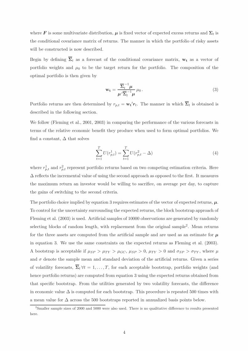
where F is some multivariate distribution, µ is fixed vector of expected excess returns and Σt is
the conditional covariance matrix of returns. The manner in which the portfolio of risky assets
will be constructed is now described.
Begin by defining Σt as a forecast of the conditional covariance matrix, wt as a vector of
portfolio weights and µ0 to be the target return for the portfolio. The composition of the
optimal portfolio is then given by
wt =Σ
−1
t µ
µ ′Σ−1
t µµ0 . (3)
Portfolio returns are then determined by rp,t = wt′rt. The manner in which Σt is obtained is
described in the following section.
We follow (Fleming et al., 2001, 2003) in comparing the performance of the various forecasts in
terms of the relative economic benefit they produce when used to form optimal portfolios. We
find a constant, ∆ that solves
T∑
t=1
U(r1p,t) =
T∑
t=1
U(r2p,t −∆) (4)
where r1p,t and r2p,t represent portfolio returns based on two competing estimation criteria. Here
∆ reflects the incremental value of using the second approach as opposed to the first. It measures
the maximum return an investor would be willing to sacrifice, on average per day, to capture
the gains of switching to the second criteria.
The portfolio choice implied by equation 3 requires estimates of the vector of expected returns, µ.
To control for the uncertainty surrounding the expected returns, the block bootstrap approach of
Fleming et al. (2003) is used. Artificial samples of 10000 observations are generated by randomly
selecting blocks of random length, with replacement from the original sample2. Mean returns
for the three assets are computed from the artificial sample and are used as an estimate for µ
in equation 3. We use the same constraints on the expected returns as Fleming et al. (2003).
A bootstrap is acceptable if µSP > µTY > µGC , µSP > 0, µTY > 0 and σSP > σTY , where µ
and σ denote the sample mean and standard deviation of the artificial returns. Given a series
of volatility forecasts, Σt ∀t = 1, . . . , T , for each acceptable bootstrap, portfolio weights (and
hence portfolio returns) are computed from equation 3 using the expected returns obtained from
that specific bootstrap. From the utilities generated by two volatility forecasts, the difference
in economic value ∆ is computed for each bootstrap. This procedure is repeated 500 times with
a mean value for ∆ across the 500 bootstraps reported in annualized basis points below.
2Smaller sample sizes of 2000 and 5000 were also used. There is no qualitative difference to results presented
here.
4

3 Forecasting the covariance matrix
The approach for generating a forecast of the covariance matrix, Σt is drawn from the recent
advances in MIDAS regressions. This methodology produces volatility forecasts directly from
a weighted average of past observations of volatility. Following from Ghysels et al. (2005) a
forecast of the conditional covariance matrix, Σt is generated by
Σt =
kmax∑
k=1
b (k,θ) Σ̂t−k (5)
where Σ̂t−k are historical estimates of the covariance matrix (the estimates used here will be
described below). In this instance, the same scalar MIDAS weights, b (k,θ) will be applied
to all elements of Σ̂t−k for each lag k. The maximum lag length kmax can be chosen rather
liberally as the weight parameters b (k,θ) are tightly parameterized. All subsequent analysis is
based on kmax = 100. Here the weights are determined by means of a beta density function
and normalized such that∑
b (k,θ) = 1. A beta distribution function is fully specified by the
2 × 1 parameter vector θ. Here θ1 = 1 meaning that only the θ2 must be estimated. The
constraint 0 < θ2 < 1 ensures that the weighting function is a decreasing function of the lag k.
The historical estimates of the covariance matrix will now be described
Σ̂t: Daily returns (D)
The estimate of the covariance matrix is simply the outer-product of the vector of daily returns,
rt
Σ̂t = rtr′
t. (6)
Σ̂t: Intraday returns (RV)
Here the estimate is the sum of the outer-product of intraday returns,
Σ̂t =N∑
i=1
ritri′
t (7)
where N represents the number of intraday intervals.
The loss functions under which values for θ2 in equation (5) is estimated will be described.
Quasi- Maximum Likelihood QML
The value for θ2 is chosen so as to
argmaxθ2
T∑
t=1
log(|Σt|) + rtΣ−1
t r′t. (8)
5

Minimum Mean Squared Error MSE
Under this estimation criteria, θ2 is chosen so as to
argminθ2
T∑
t=1
vec(Σt − Σ̂t)′ vec(Σt − Σ̂t). (9)
Utility Based Estimation UTL
Skouras (2007) proposes a method by which the parameters of a univariate volatility model
can be estimated directly within an economic criteria. As opposed to likelihood maximization,
Skouras (2007) suggests estimating parameters by maximizing the utility realized from the
portfolios formed from model forecasts.
Given the optimal portfolio rule in equation (3), and the expression for realized utility in equa-
tion (1), the objective function for a maximum utility estimator is
argmaxθ2
1
T
T∑
t=1
− exp(−λwt′rt). (10)
Parameter estimation is conducted on the basis of optimally weighting historical volatility so
as to construct portfolios that lead to the greatest expected utility as opposed to statistically
optimal forecasts of volatility.
4 Data
The portfolio allocation problem considered here relates to a mix of bond, equities and gold.
The study treats returns on S&P 500 Composite Index futures as equities exposure (SP), returns
on U.S. 10-year Treasury Note futures as bond market exposure (TY) along with returns on
Gold futures (GC) 3. Data was gathered for the period covering 1 July 1997 to 29 June 2009
giving a sample of 2985 observations. RV estimates of the covariance matrix were constructed
by summing the cross products of 15 minute futures contract returns.
Table 1 reports the means and standard deviations of each of the individual elements in the
covariance matrix. Panel A reports on the covariance estimates where Σ̂t: D and Panel B, Σ̂t:
RV. It is clear from comparing the means, that on average both the daily (D) and RV estimates
are virtually indistinguishable from each other. A comparison of the standard deviations in
the right hand columns reflect the well know pattern that more precise volatility estimates
are obtained by using high frequency intraday returns. In most cases the standard deviations
of the daily based volatility estimates are 50% larger than the corresponding RV estimates.
The greater precision of RV normally leads to improved forecasts and portfolio outcomes. This
3Intraday data for both futures contracts were purchased from Tick Data
6

Mean×10−3 Standard Deviation×10−3
Panel A: Σ̂t: D
SP TY GC SP TY GC
SP 0.1741 -0.0153 -0.0037 SP 0.6223 0.0944 0.2428
TY - 0.0171 0.0042 TY - 0.0389 0.0644
GC - - 0.1328 GC - - 0.3551
Panel B: Σ̂t: RV
SP TY GC SP TY GC
SP 0.1712 -0.0170 -0.0020 SP 0.4455 0.0666 0.1591
TY - 0.0159 0.0028 TY - - 0.0397
GC - - 0.1366 GC - - 0.3452
Table 1: Means and standard deviations of the individual elements in the historical estimates
of the covariance matrix. Panel A show results for Σ̂t given daily returns, and Panel B intraday
returns.
widely held belief will be reconsidered in light of altering the loss function under which volatility
forecasts are generated.
S&P 500 realized volatility
Treasury bond realized volatility
Gold realized volatility
1999 2001 2003 2005 20070
0.002
0
0.0003
0
0.005
Figure 1: S&P 500 RV estimates (top panel), Treasury bond RV estimates (middle panel) and
Gold RV estimates (bottom panel).
Figures 1 and 2 plot the realized volatilities and correlations of the three assets considered4.
Figure 1 shows the realized volatility of equity futures (top panel), bond futures returns (middle
4Correlations are shown as they are easier to interpret. Volatility estimates using daily returns are not shown
as they are simply a more noisy estimate relative to the RVs shown here.
7

S&P 500 - Treasury bond realized correlation
S&P 500 - Gold realized correlation
Treasury bond - Gold realized correlation
1999 2001 2003 2005 2007-1
1
-1
1
-1
1
Figure 2: S&P 500 and RV Treasury bond realized correlation estimates (top panel), S&P 500
and Gold realized correlation estimates (middle panel) and Treasury bond and Gold realized
correlation estimates (bottom panel).
panel) and gold futures returns (lower panel). Equity volatility shows a familiar pattern, low
volatility during much of the sample period with higher volatility due to collapse of technology
stocks. It is clear that the events surrounding the credit crisis of the second half of 2008
dominate in terms of the levels of volatility reached (the scale of the plot has been constrained
otherwise no variation is evident due to the level of recent volatility). The volatility of bond
returns is unsurprisingly much lower in magnitude than equity returns and generally more
stable. It is evident that the recent financial crisis has lead to a sustained period of somewhat
higher volatility. Volatility in gold returns rose in late 2005 and early 2006 due to central bank
activity, and rose to historically high levels due the height of the recent market turmoil.
Realized correlations between the respective pairs of assets are shown in Figure 2. The correla-
tion between equities and bonds (top panel) is quite persistent over time. It shows a downward
trend through to 2002-2003 with it subsequently being weak during 2004-2006, followed by a
period very strong negative correlation during much of the recent crisis. In contrast to the bond
and equity case, neither the correlation between either equities and gold (middle panel) nor
bonds and gold (lower panel) show any long-term persistence or structure.
8
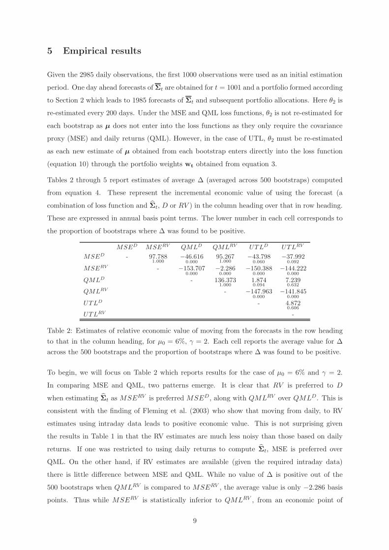
5 Empirical results
Given the 2985 daily observations, the first 1000 observations were used as an initial estimation
period. One day ahead forecasts ofΣt are obtained for t = 1001 and a portfolio formed according
to Section 2 which leads to 1985 forecasts of Σt and subsequent portfolio allocations. Here θ2 is
re-estimated every 200 days. Under the MSE and QML loss functions, θ2 is not re-estimated for
each bootstrap as µ does not enter into the loss functions as they only require the covariance
proxy (MSE) and daily returns (QML). However, in the case of UTL, θ2 must be re-estimated
as each new estimate of µ obtained from each bootstrap enters directly into the loss function
(equation 10) through the portfolio weights wt obtained from equation 3.
Tables 2 through 5 report estimates of average ∆ (averaged across 500 bootstraps) computed
from equation 4. These represent the incremental economic value of using the forecast (a
combination of loss function and Σ̂t, D or RV ) in the column heading over that in row heading.
These are expressed in annual basis point terms. The lower number in each cell corresponds to
the proportion of bootstraps where ∆ was found to be positive.
MSED MSERV QMLD QMLRV UTLD UTLRV
MSED - 97.7881.000
−46.6160.000
95.2671.000
−43.7980.060
−37.9920.092
MSERV - −153.7070.000
−2.2860.000
−150.3880.000
−144.2220.000
QMLD - 136.3731.000
1.8740.094
7.2390.632
QMLRV - −147.9630.000
−141.8450.000
UTLD - 4.8720.606
UTLRV -
Table 2: Estimates of relative economic value of moving from the forecasts in the row heading
to that in the column heading, for µ0 = 6%, γ = 2. Each cell reports the average value for ∆
across the 500 bootstraps and the proportion of bootstraps where ∆ was found to be positive.
To begin, we will focus on Table 2 which reports results for the case of µ0 = 6% and γ = 2.
In comparing MSE and QML, two patterns emerge. It is clear that RV is preferred to D
when estimating Σ̂t as MSERV is preferred MSED, along with QMLRV over QMLD. This is
consistent with the finding of Fleming et al. (2003) who show that moving from daily, to RV
estimates using intraday data leads to positive economic value. This is not surprising given
the results in Table 1 in that the RV estimates are much less noisy than those based on daily
returns. If one was restricted to using daily returns to compute Σ̂t, MSE is preferred over
QML. On the other hand, if RV estimates are available (given the required intraday data)
there is little difference between MSE and QML. While no value of ∆ is positive out of the
500 bootstraps when QMLRV is compared to MSERV , the average value is only −2.286 basis
points. Thus while MSERV is statistically inferior to QMLRV , from an economic point of
9

view, there is little difference between the value of the two loss functions when RV is used. This
finding has interesting implications for how a volatility model is estimated. From equation 8
is clear that the inverse of Σt must be taken. Computationally this becomes a difficult issue
when the dimension of the portfolio becomes large which in a practical setting is often the
case. The fact that (when using RV) MSE leads to virtually the same economic outcome is an
important finding in that larger dimensional problems can be handled using MSE avoiding the
computational issues associated with QML. UTLD and UTLRV are inferior to both MSED
and MSERV but approximately equivalent in performance to QMLD. Skouras (2007) finds
that UTL is superior to QML, but only in a univariate setting using daily returns and does not
consider the performance of MSE.
MSED MSERV QMLD QMLRV UTLD UTLRV
MSED - 107.2881.000
−64.1150.000
103.5141.000
−58.3770.064
−54.3700.104
MSERV - −194.2980.000
−3.0690.000
−186.3640.000
−180.7660.000
QMLD - 154.7431.000
1.5670.156
2.6350.624
QMLRV - −183.4130.000
−178.3820.000
UTLD - 0.7290.658
UTLRV -
Table 3: Estimates of relative economic value of moving from the forecasts in the row heading
to that in the column heading, for µ0 = 6%, γ = 5. Each cell reports the average value for ∆
across the 500 bootstraps and the proportion of bootstraps where ∆ was found to be positive.
MSED MSERV QMLD QMLRV UTLD UTLRV
MSED - 133.1011.000
−67.6180.000
129.3501.000
−62.5100.064
−55.2210.084
MSERV - −217.1890.000
−3.3160.000
−211.0230.000
−202.9880.000
QMLD - 187.3301.000
3.1150.110
9.4070.634
QMLRV - −207.5310.000
−199.6340.000
UTLD - 5.5650.596
UTLRV -
Table 4: Estimates of relative economic value of moving from the forecasts in the row heading
to that in the column heading, for µ0 = 8%, γ = 2. Each cell reports the average value for ∆
across the 500 bootstraps and the proportion of bootstraps where ∆ was found to be positive.
Tables 3 through 5 report average ∆ for increasing µ0 and, or γ. Overall, the results in terms
of rankings discussed earlier remain the same. The differences in economic value reflected in
the average value for ∆ become greater in absolute terms, a pattern also observed in Fleming
et al. (2003). There are three combinations where there is little difference between the economic
value of the forecasts, QMLRV and MSERV , UTLD and QMLD and UTLD and UTLRV . In
these cases only relatively minor changes in average ∆ occur as µ0 or γ increase and hence the
10

forecasts continue to perform in a very similar manner.
MSED MSERV QMLD QMLRV UTLD UTLRV
MSED - 150.6801.000
−97.2060.000
144.8101.000
−87.7240.056
−86.9350.112
MSERV - −288.3660.000
−4.4910.000
−274.1930.000
−269.5340.000
QMLD - 219.7881.000
0.0300.200
−8.9380.536
QMLRV - −270.4700.000
−267.9780.000
UTLD - −8.5650.660
UTLRV -
Table 5: Estimates of relative economic value of moving from the forecasts in the row heading
to that in the column heading, for µ0 = 8%, γ = 5. Each cell reports the average value for ∆
across the 500 bootstraps and the proportion of bootstraps where ∆ was found to be positive.
In practice, an investor faces transaction costs as they alter their portfolio holdings through
time. These costs are a function of both the frequency and magnitude of portfolio changes.
Here we do not take a stance on the form of the transaction costs but compare the mean
absolute changes in portfolio weights and their standard deviations, to reveal whether a link
exists between the competing forecasts and portfolio stability. These statistics are reported
in Table 6. There is little difference between whether D or RV estimates are used under the
MSE loss function. The magnitude and volatility of portfolio changes are quite similar for both
MSED and MSERV across the three asset classes. However, when one moves to QML or UTL,
the magnitude and volatility of changes in weights generally increase by 50% to nearly 100%.
Overall, MSE (irrespective of the data used to estimate Σ̂t) produces the most stable forecasts
and hence portfolio weights, which in practice minimizes transaction costs.
MSED MSERV QMLD QMLRV UTLD UTLRV
|∆wSP| 0.0303 0.0318 0.0570 0.0384 0.0524 0.0518
σ∆wSP0.0364 0.0381 0.0642 0.0454 0.0613 0.0602
|∆wTY| 0.0487 0.0514 0.0905 0.0619 0.0815 0.0827
σ∆wTY0.0568 0.0590 0.0988 0.0701 0.0931 0.0930
|∆wGC| 0.0344 0.0332 0.0633 0.0398 0.0570 0.0568
σ∆wGC0.0420 0.0384 0.0729 0.0452 0.0675 0.0669
Table 6: Mean absolute changes and standard deviation of changes in exposures to equities
(wSP ), bonds (wTY ) and gold (wGC).
6 Conclusion
Forecasts of volatility are important in many aspects of finance, and as such this literature has
grown substantially in recent years. In recent years it has been shown that by harnessing high
frequency returns, superior estimates of volatility can be produced. Such estimates, commonly
11

known as realized volatility, are often used for forecasting volatility and lead to superior portfolio
allocation outcomes. Traditionally, the parameters of volatility models are estimated within a
maximum likelihood framework, and the forecasts they generate are often used, or evaluated in
economic applications such as portfolio allocation.
While it is well known that realized volatility is the preferred approach for estimating volatility
itself, less is understood about whether the loss function under which model parameters are
estimated is important. In this paper we address this issue, and in doing so examine whether
realized volatility is still preferred under alternative estimation schemes. We find that while
realized volatility based on high frequency data is preferred over simply using daily returns, the
loss function under which model parameters are estimated is also important. Using realized
volatility, there is little difference in the economic benefit produced under either maximum
likelihood or simple mean squared error loss functions. Portfolios generated from forecasts
produced under mean squared error are also found to be more stable, an important finding
given the impact of transactions costs. From a practical point of view, a means squared error
approach also avoids the computation issues of evaluating a multivariate likelihood function
when the dimension of the portfolio becomes large.
References
T. G. Andersen, T. Bollerslev, F. X. Diebold, and P. Labys. The distribution of realized exchange
rate volatility. Journal of the American Statistical Association, 96(453):42–55, 2001.
T.G. Andersen, T. Bollerslev, F.X. Diebold, and P. Labys. Modeling and forecasting realized
volatility. Econometrica, 71:579–625, 2003.
T.G. Andersen, T. Bollerslev, P.F. Christoffersen, and F.X. Diebold. Volatility and correlation
forecasting. In G. Elliot, C.W.J. Granger, and A. Timmerman, editors, Handbook of Economic
Forecasting. Elsevier, Burlington, 2006.
O.E. Barndorff-Nielsen and N. Shephard. Econometric analysis of realized volatility and its use
in estimating stochastic volatility models. Journal of Royal Statisitcal Society, Series B, 64:
253–280, 2002.
R. Becker and A. Clements. Are combination forecasts of s&p 500 volatility statistically superior.
The International Journal of Forecasting, 24:122–133, 2008.
T. Bollerslev. Generalized autoregressive conditional heteroskedasticity. Journal of Economet-
rics, 31:307–327, 1986.
12
T. Bollerslev. Modelling the coherence in short-run nominal exchange rates: A multivariate
generalized arch model. Review of Economics and Statistics, 72:498–505, 1990.
J. Y. Campbell, A. W. Lo, and A. G. Mackinlay. The Econometrics of Financial Markets.
Princeton University Press, Princeton, 1997.
M.M. Copeland and T.E. Copeland. Market timing: Style and size rotation using vix. Financial
Analysts Journal, 55:73–81, 1999.
R.F. Engle. Autoregressive conditional heteroskedasticity with estimates of the variance of
united kingdom inflation. Econometrica, 50:987–1008, 1982.
R.F. Engle. Dynamic conditional correlation. a simple class of multivariate generalized autore-
gressive conditional heteroskedasticity models. Journal of Business and Economic Statistics,
20:339–350, 2002.
J. Fleming, C. Kirby, and B. Ostdiek. The economic value of volatility timing. The Journal of
Finance, 56:329–352, 2001.
J. Fleming, C. Kirby, and B. Ostdiek. The economic value of volatility timing using realized
volatility. Journal of Financial Economics, 67:473–509, 2003.
E. Ghysels, P. Santa-Clara, and R. Valkanov. There is a risk-return trade-off after all. Journal
of Financial Economics, 76:509–548, 2005.
C. Gourieroux and J. Jasiak. Financial Econometrics. Princeton University Press, Princeton,
New Jersey, 2001.
J.R. Graham and C.R. Harvey. Market timing ability and volatility implied in investment
newsletters’ asset allocation recommendations. Journal of Financial Economics, 42(3):397–
421, 1996.
P.R. Hansen and A. Lunde. A forecast comparison of volatility models: Does anything beat a
garch(1,1)? Journal of Applied Econometrics, 20:873–889, 2005.
S-H. Poon and C. W. J. Granger. Forecasting volatility in financial markets: a review. Journal
of Economic Literature, 41:478–539, 2003.
S-H. Poon and C. W. J. Granger. Practical issues in forecasting volatility. Financial Analysts
Journal, 61:45–56, 2005.
G.W. Schwert. Does stock market volatility change over time? Journal of Finance, 44:1115–
1153, 1989.
13

S. Skouras. Decisionmetrics: A decision-based approach to economic modelling. Journal of
Econometrics, 137:414–440, 2007.
K.D. West, H.J. Edison, and D. Cho. A utility-based comparison of some models of exchange
rate volatility. Journal of International Economics, 35:23–45, 1993.
14