1

Volatility Based Sentiment Indicators for Timing the Markets

School of Economics and Management

Lund University

Master Thesis of Finance

Fabio Cacia 670715 - 0352

Rossen Tzvetkov 830504 – T116

Abstract: VIX, published by the Chicago Board Options Exchange, is a well known

implied volatility estimator. In this paper we assess its capability to be used as a

sentiment indicator, and to give signals for a short term investment strategy. It will be

proved and discussed how VIX-based strategies – also known as “Contrarian” strategies

– can be effective as they lead to higher returns than the market. We also propose a purer

sentiment indicator derived from VIX that gives more accurate market timing signals. We

call this indicator “Net Emotional Volatility Index” (NEVI). It proves to have interesting

properties, a highly significant statistical relationship with the market return, and a

considerable power to time the market. The results of our back-testing for the period

2001-2002 and 2006-2007 using the two indicators are presented, compared and

discussed. Possible explanations of the information that NEVI brings and why its signals

work are provided.

Key words: VIX, GARCH, market timing signals, sentiment, volatility

Supervisors: Hossein Asgharian – Björn Hansson

2

Table of Contents

1 Introduction 3

2. Contrarian Sentiment Indicator – Implied Volatility Index 4

2.1. Contrarian Investing 4

2.2 Implied Volatility Index (VIX) 4

3. NEVI (Net Emotional Volatility Index) 8

4. Data Set and Regression Analysis 12

5. Comparing VIX and NEVI Investment Strategies 17

5.1 Contrarian Strategy Based on VIX 17

5.2 Momentum Strategy Based on NEVI 22

6. Interpretation of the Indicators 24

6.1 NEVI is a Pure Sentiment Indicator 24

6.2 Institutional Investors Lead the Market 25

7.0 Conclusion 26

Appendix 27

References 31

3

1. Introduction

Volatility is a major factor in the financial markets and volatility forecasts are

used every day in the process of portfolio choice, risk management, hedging and pricing.

The goal of this paper is to assess the capability of volatility based indicators to

measure investors’ sentiment, to time the markets and to give signals for a short term

investment strategy. First, we address this problem by studying the signaling quality of

the famous “Contrarian” indicator VIX (Implied Volatility Index). Second, we propose a

completely new volatility based indicator, NEVI (Net Emotional Volatility Index),

defined as the difference between VIX and a GARCH (1,1) forecast over the same time

horizon, which according to us has a higher signaling power in a certain market

environment.

The market timing power of the two indicators is examined both with the use of

regressions and with the help of out-of-sample investment strategies back-testing based

on their signals. In the case of VIX, we utilize a “Contrarian” strategy, where we take

positions contrary to the general market sentiment. We use NEVI, instead, in what we

called a “Sentiment Momentum Strategy”, where we follow the people’s expectations.

The usefulness of both indicators for predicting the market direction is tested in two

historical periods. The first one is 2001-2002, when the market was comparatively more

volatile, and the second one is 2006-2007, when the market was less volatile. This gives

us a better idea of the behavior of the two indicators.

The work is organized as follows. In the first part we briefly present the

“Contrarian” investment philosophy and introduce VIX, giving an overview of its

characteristics and properties. In the second part we introduce and define the NEVI

indicator, arguing why it might be a purer sentiment measure and a better market timing

indicator. In the third part we present the data series that we work with, and conduct a

regression analysis for both VIX and EVI, proving that one is a “Contrarian” indicator,

while the other is a “Momentum” indicator. In the next part of the work we explain the

investment strategies based on the two indicators and present the results. Finally we give

two explanations why the Net Emotional Volatility Indicator NEVI works.

4

2. Contrarian Market Sentiment Indicator - Implied Volatility Index

2.1. Contrarian Investing

“Contrarian” investing is an investment philosophy that is closely related to the

field of behavioral finance. It is followed by those investors who believe that the crowd

behavior is typical for the market participants and that it often leads to the mispricing of

the traded assets. Some “Contrarian” strategies have gained a considerable popularity

among agents as they are widely believed to be able to time when the markets are going

to change directions. The basis of any “Contrarian” strategy is to recognize when the

majority of the market participants have become too extreme in their optimism or fear. At

such occasion the “Contrarian” investors normally open positions against the general

market trend, as they believe that market reversal will follow.

Taking the right side at the top or the bottom of the market leads to high returns

but determining whether the market is excessively bullish or bearish is not an easy task.

There exist a large number of market characteristics that are thought to be signs of

overbought or oversold markets. For example the extremely low values of the Put-Call

Ratio (indicator derived by dividing the number of the traded put options to the number

of call options) can be interpreted as an overbought market, while the high values of the

indicator are usually perceived as an alarm that the market is oversold. The fully invested

portfolios of the mutual funds can also be used as an indication that the market might

have surpassed its potential and that a drop in prices is to follow. In such cases the good

news coming to the market do not have a big effect since all the money are already

invested, while the bad news can cause a sale. It can turn out very profitable for every

investor to be able to measure the market sentiment and use this as a weapon in his or her

trading arsenal.

2.2. Implied Volatility Index (VIX)

VIX is an index that measures the implied volatility conveyed by the option

prices. When the option prices and all other option pricing factors, but volatility, are

5

known, the implied volatility is derived with a reverse calculation using a mathematical

model. VIX was introduced in 1993 by the CBOE and originally it was based on the

Black-Scholes option pricing model, considering only at-the-money put and call options

on the S&P 100 index with a residual life of 30 days. Soon after its introduction in 1993,

the VIX was widely accepted as a benchmark for stock market volatility.

In September 2003, the CBOE changed the formula it uses to calculate the VIX,

in an attempt to come up with a more accurate gauge of the expected market volatility.

The new VIX is not any longer based on the Black-Scholes OPM, but uses a newly

developed formula1:

∑=

−−

∆

to

tRT

t

tT

K

F

TKQe

K

K2

2

21

1)(

2σ

Where,

σ is 100

VIX, meaning that VIX = σ x 100

T is Time to expiration. Precisely:

T = {M Current day + M Settlement day + M Other days}/ Minutes in a year

Where M Current day = # of minutes remaining until midnight of the current day

M Settlement day = # of minutes from midnight until 8:30 a.m. on settlement day

M Other days = Total # of minutes in the days between current day and

settlement day.

F is the Forward index level derived from at-the-money index option prices2

K i is the Strike price of i th out-of-the-money option; a call if K i >F and a put if

Ki<F

1 Details on the formula and relevant calculations are available at:

http://www.cboe.com/micro/vix/vixwhite.pdf

2 F=Strike Price + e )PrPr( icePuticeCallRT −∗ . The at-the-money Strike Price is the

strike price at which the difference between the call and put prices is smallest.

6

∆Ki is the Interval between strike prices – half the distance between the strike on

either side of K i : iК∆ = 2

K- K 1-i1i+ . ( К∆ for the lowest strike is simply the

difference between the lowest strike and the next higher strike, Likewise, К∆ for

the highest strike is the difference between the highest strike and the next lower

strike.)

K0- First strike below the forward index level, F

R – Risk-free interest rate of expiration

Q(K i ) – The midpoint of the bid-ask spread for each option with strike K i .

The new VIX incorporates data from prices of options with a wide variety of

strikes, capturing the whole volatility skewness. It is based on S&P 500 index, instead of

the S&P 100. The old VIX is now called VXO. It continues to be estimated only with the

help of at-the-money options on the S&P 100 index. The new VIX has been re-calculated

from 1993 in order to insure data homogeneity. The changes are not insignificant but the

basic idea of the volatility index remains the same. It is a measure of the expected market

volatility over a 30 day time horizon.

There are many papers focusing on volatility forecasting methods, where VIX is

considered to be the main expression of what is defined as implicit volatility, and its

capability to forecast realized volatility is compared to that of other methods such as

historical based volatility and Model Based Forecast (especially GARCH). Results are

different and often contradictory.

Blair, Poon, and Taylor (2001)3 compare historical methods with VIX and find

that not much incremental information is provided by the former in comparison with the

3 Blair, B.J., S. Poon, and S.J. Taylor, 2001, Forecasting S&P100 volatility: the

incremental information content of implied volatilities and high-frequency index returns,

Journal of Econometrics 105, 5–26.

7

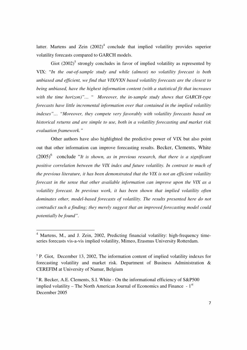
latter. Martens and Zein (2002)4 conclude that implied volatility provides superior

volatility forecasts compared to GARCH models.

Giot (2002)5 strongly concludes in favor of implied volatility as represented by

VIX: “In the out-of-sample study and while (almost) no volatility forecast is both

unbiased and efficient, we find that VIX/VXN based volatility forecasts are the closest to

being unbiased, have the highest information content (with a statistical fit that increases

with the time horizon)”… “ Moreover, the in-sample study shows that GARCH-type

forecasts have little incremental information over that contained in the implied volatility

indexes”… “Moreover, they compete very favorably with volatility forecasts based on

historical returns and are simple to use, both in a volatility forecasting and market risk

evaluation framework.”

Other authors have also highlighted the predictive power of VIX but also point

out that other information can improve forecasting results. Becker, Clements, White

(2005)6 conclude “It is shown, as in previous research, that there is a significant

positive correlation between the VIX index and future volatility. In contrast to much of

the previous literature, it has been demonstrated that the VIX is not an efficient volatility

forecast in the sense that other available information can improve upon the VIX as a

volatility forecast. In previous work, it has been shown that implied volatility often

dominates other, model-based forecasts of volatility. The results presented here do not

contradict such a finding; they merely suggest that an improved forecasting model could

potentially be found”.

4 Martens, M., and J. Zein, 2002, Predicting financial volatility: high-frequency time-

series forecasts vis-a-vis implied volatility, Mimeo, Erasmus University Rotterdam.

5 P. Giot, December 13, 2002, The information content of implied volatility indexes for

forecasting volatility and market risk. Department of Business Administration &

CEREFIM at University of Namur, Belgium

6 R. Becker, A.E. Clements, S.I. White - On the informational efficiency of S&P500

implied volatility – The North American Journal of Economics and Finance - 1st

December 2005

8

All these papers are focused on the predictive power of the indicator and are

concerned with the efficiency and unbiasedness of the volatility estimator. For our work

we will change the focus towards the research of a reliable indicator for timing the

market and for implementing a short term portfolio investment strategy.

Many investors tend to view VIX just as a tool for measuring the market fear.

During times of financial distress and general market insecurity, when stock prices

usually decline, VIX is normally expected to rise. The greater the market risks, the higher

the index would rise. Such behavior of VIX is clearly due to the riskier conditions in the

market, since volatility is the most common measure of risk. It is amplified by the

hedging actions of the market participants, which include the use of options. Such

demand for options leads to an increase of their premiums and so VIX rises.

Many “Contrarian” investors believe that the bottoms of the VIX value translate

into tops in the market, and the tops of the VIX index coincide with the bottoms in the

market. It is widely believed among them that when the implied volatility is extremely

high the market is shaking in fear and it is a good moment to buy, while when the implied

volatility is too low the agents are too optimistic and it is a good moment to sell.

When the investors’ reaction to a particular bad event is too strong due to excess

fear, the market will drop more than reasonable. However, with the time, market

participants will assess the market conditions more carefully and the mispricing will be

corrected. On the other hand, if the majority of investors are overoptimistic and do not

react to a really bad event, or overprice the effect of good news, later they will realize

their mistake and the market will go down as a result.

3.0. NEVI (Net Emotional Volatility Index)

The investors that blindly follow the VIX signals are likely to make mistakes

from time to time. By taking long positions when VIX has extremely high values for

example, they take it for granted that the majority of the investors overreact and that the

market will have a correction soon. However the only reason to believe that markets are

overreacting is that VIX climbs high above/falls low below the average values of the

9

indicator. In our opinion extreme values of the implied volatility can be a result of both

the behavior of the investors or the properties of the volatility itself, so that not all VIX

signals might be accurate sentiment alarms, while at the same time VIX might miss some

good market opportunities. We can neither be sure when the investors are overreacting

and if their fears are unreasonable or rational, nor be sure how long it will take them to

realize and correct their irrational behavior. However we can try to estimate how big their

fear or optimism actually is.

We argue that high VIX does not automatically translate into (unreasonably) high

fear and for that reason we propose a new and more reliable sentiment market timing

indicator based on volatility forecasts. We created an indicator that we called Net

Emotional Volatility Index (NEVI). This indicator is a proxy for the sentiment of the

investors. It is calculated as the difference between the market based implied volatility

VIX and the model-based forecast over the same period ((GARCH (1,1) forecast)). We

argue that this indicator is a purer sentiment gauge than VIX alone is.

GARCH (1,1) (Generalized Autoregressive Conditionally Heteroscedastic) model

is an econometric tool for modeling time-varying conditional variances. It is

acknowledged for being able to account for volatility clustering and excess kurtosis, and

is widely recognized for providing accurate forecast of return volatility. Usually, it is

found that a GARCH (1,1) model is sufficient to capture the volatility dynamics7, so that

only one lagged squared error and one lagged variance is needed:

2

1

2

1

2

−− ++= ttt βσαηωσ

Considering the widely recognized properties of GARCH (1,1), and after

obtaining a positive result with the test for ARCH/GARCH effect on the S&P 500

sample, we decided to use this model in our research.

As good as GARCH (1,1) is, it suffers from several limitations. Since the

GARCH models are conditional and autoregressive, the forecasts are dependent on the

observations of the immediate past, and past observations are incorporated into the

present. As any econometric model, the GARCH forecast follows a mathematical pattern.

7 See “Empirical Finance Lecture Notes Part 1”, Fall 2007, by Hossein Asgharian, Associate Professor at

Lund University, Sweden.

10

The parametric characteristic of the model leads to a better performance when the market

conditions are comparatively stable. To forecast volatility for the next 30 days, for

example, GARCH models reiterate the calculation and tomorrow’s forecast becomes the

last observation in the time series to forecast volatility for the day after tomorrow, and so

on. Since the forecasts are smoothed by the past observations, the model needs a certain

time to account for the unanticipated volatility jumps and when a shock is registered it

takes a certain number of observations for the model to capture the change.

Implied volatility on the other hand includes information known by the market

agents about the historical behavior of the volatility but it includes also the sentiment of

the option traders with regards to the development of the volatility in the near future.

Therefore the VIX value incorporates the volatility forecast based on the historical

volatility pattern, as well as the volatility expectations of the investors, resulting from

their emotional reaction to the current market environment. In our opinion the GARCH

(1,1) forecast can be considered as a proxy for the volatility that the option traders expect

based on the historical behavior of the market. The implied volatility is obtained by

adding the emotional reactions and the expectations of the investors, based on the current

market events and phenomena, to the model based forecast. Our theory finds support in

the recent work of Becker, Clements and McClelland (BCM) (2008)8, who argue that as a

market determined forecast, VIX can reflect information that cannot be captured by a

model based forecast. In addition they also show that VIX have incremental information

in comparison to a Model Based Forecast (MBF), when it comes to explaining future

jump activity. This is the part of volatility that we call emotional. Our intuition is that a

good proxy for the emotional volatility is the difference between the market determined

volatility forecast VIX and a model based volatility reiterated forecast as presented by a

GARCH (1,1) model.

Daily VIX fixing takes into account the historical volatility trend, the volatility

clustering effect, and the everyday news and events that can affect the emotions and

expectations of the option traders as well. Conversely a model based forecast, like

8 Ralf Becker, Adam Clements and Andrew McClelland; “The Jump Component of S&P 500 volatility and

the VIX index”, March 2008

11

GARCH (1,1), can capture the first two components but not the latter (at least not

immediately). Corporate news and economic indicators, political changes and

technological innovations, natural disasters and terrorist attacks instantly affect the

attitude of the investors (optimism, pessimism) and as a result the implied volatility

(VIX) moves accordingly. Market events that are expected to happen or are happening

suddenly at the moment can change the perception of the investors about the recent or

more distant price changes, as well as their expectations about the future. On the contrary

a model based forecast, is much more dependent and smoothed by the past, and as a

result the forecast reacts relatively slower to expected jumps in the market. The reason

for that is that the coefficients of the model are estimated on the basis of many years of

observations. To obtain a forecast for tomorrow these coefficients are applied to today’s

volatility and to today’s difference between the market actual return and the return

expressed by a mathematical model. Therefore, given a shock that is able to affect the

S&P 500, the change in the S&P volatility forecast for tomorrow will be transmitted

through today’s change in the return, as error with respect to a mathematical model, and

through today’s registered volatility. Both components will be weighted by β, α, and will

also stand the effect of the coefficient ώ. We could say that shock impacts are “filtered”

and such filtering becomes stronger when we use GARCH models with reiteration of

forecasts (when we use tomorrow’s forecast as a base for the forecast for the day after

tomorrow and so on, like what we do in the following section)). The final output of a 30

days GARCH (1,1) reiterated forecast is surely less affected by today’s shocks, news, and

events and by the relevant emotional reactions of the market agents, than what could be

the volatility implicitly assumed by the options traders. The latter, and so VIX , is

certainly more directly responding to the above mentioned factors since shocks’ effects

are not “filtered” to obtain the forecast. Given that the other variables involved in the

option pricing model are not changed we just plug the new market price in the formula

and through a reverse calculation we get the implicit volatility. This insures a much faster

reactions of the implied volatility to the market shocks.

For our purposes, this argument - that could be a drawback of GARCH models in

other researches - could actually become a useful advantage. The difference between the

12

two volatility values can be a good proxy of the reactions of the market agents to today’s

events, news, and shocks. This is what we call emotional volatility.

According to our arguments above, VIX can be decomposed into two parts –

rational market volatility and emotional volatility. The emotional volatility derived from

VIX is a purer sentiment indicator than VIX itself is, and it can probably be used more

successfully in an investment strategy. To our best knowledge, no one has ever discussed

in the literature before the indicator that we created and named Net Emotional Volatility

Index (NEVI).

4. Data Set and Regression Analysis

We have gathered daily closing values of the VIX for the period January 1997 –

December 2007. We set two estimation windows, 1997-2000 and 1997-2005, to measure

the statistic properties of the indicator, and two event windows, 2001-2002 and 2006-

2007 respectively, which are used in the following sections for a back-testing analysis of

the portfolio strategies based on VIX.

The resulting statistical properties for VIX in the two estimation windows are presented

below in Table 1.

Table 1. Statistical Properties of VIX for the period 1997-2000 and 1997-2005

Deciles Period 1997-2000 Deciles Period 1997-2005

0.1 19.23 Mean 23.91 0.1 13.57 Mean 22.099

0.2 20.1 Median 22.94 0.2 16.54 Median 21.5

0.3 21.04 Standard Deviation 4.692 0.3 19.02 Standard Deviation 6.463

0.4 21.9 Sample Variance 22.015 0.4 20.22 Sample Variance 41.779

0.5 22.91 Kurtosis 3.389 0.5 21.5 Kurtosis 0.500

0.6 24.03 Skewness 1.564 0.6 22.85 Skewness 0.629

0.7 25.08 Range 29.51 0.7 24.52 Range 35.51

0.8 27.01 Minimum 16.23 0.8 27.11 Minimum 10.23

0.9 29.48 Maximum 45.74 0.9 30.78 Maximum 45.74

13

Afterwards, we addressed the empirical estimation of the above described NEVI.

We proceeded subtracting the average of GARCH (1,1) forecasts for the next 30 days

from each value of the VIX times series. Precisely, we built a GARCH (1,1) model

starting from the observations of S&P 500 in two estimation windows, 1997-2007 and

1997-2002. Then we used these models to forecast volatility for the periods 2001-2002

and 2006-2007. It is worth noting that just for the GARCH coefficients we used enlarged

estimation windows and therefore we output an “in sample” forecast. We believe that this

is the best solution for our back-testing purposes, since an “out of sample” forecasting,

that normally sounds more rigorous, in this case would cause a bigger approximation,

making simulations more distant from reality. In reality, in fact, every agent can daily

recalculate and update his/her GARCH Model. An “out of sample” forecasting, instead,

would create a simulation in which the agents cannot update their GARCH models.

The coefficients are presented in Table 2 below.

Table 2: GARCH (1,1) Coefficients

Garch Coefficients ω α β

1997-2007 0,0000012 0,070164 0,922884

1997-2002 0,0000093 0,098557 0,851944

Once the GARCH coefficients are obtained, for each day we forecast the

volatility for the next 30 days, reiterating the forecast, which means that every forecast

becomes the last observation for the next forecast. Finally we take the average of these

values. We call this Average GARCH Forecast (AGF).

The difference between VIX and AGF is what we already called Net Emotional

Volatility Index (NEVI). It is normally positive, with a positive mean and median value.

Below in table 3 are presented the Histogram, the Deciles distribution and other statistical

properties for NEVI in two estimation windows 1997-2000 and 1997-2005 9:

9 Estimation windows now are 2 years shorter than the ones used to estimate GARCH coefficients,

therefore exactly equal to the ones used for VIX. Deciles and other NEVI statistical properties measured

in such estimation windows will be used in the following sections for back-testing analysis of NEVI based

portfolio strategies in the event windows, 2001-2002 and 2006-2007.

14

Table 3. Statistical Data for NEVI

Deciles Period 1997-2005 Deciles Period 1997-2000

0.1 -0,76% Mean 0.0361 0.1 -0,64% Mean 0.0297

0.2 0,55% Median 0.0333 0.2 0,08% Median 0.0216

0.3 1,71% Standard Deviation 0.0376 0.3 0,75% Standard Deviation 0.0362

0.4 2,48% Sample Variance 0.0014 0.4 1,43% Sample Variance 0.0013

0.5 3,33% Kurtosis 1.3161 0.5 2,16% Kurtosis 2.5768

0.6 4,21% Skewness 0.4047 0.6 3,06% Skewness 1.2633

0.7 5,29% Range 0.3221 0.7 4,20% Range 0.2695

0.8 6,51% Minimum -0.092 0.8 5,56% Minimum -0.056

0.9 8,37% Maximum 0.2302 0.9 7,87% Maximum 0.213

0%

20%

40%

60%

80%

100%

120%

0

20

40

60

80

100

120

140

160

Fre

qu

en

cy

Histogram 1997 - 2000

0%

20%

40%

60%

80%

100%

120%

0

50

100

150

200

250-0

,09

19

64

20

7

-0,0

71

40

20

53

-0,0

50

83

98

99

-0,0

30

27

77

45

-0,0

09

71

55

91

0,0

10

84

65

63

0,0

31

40

87

17

0,0

51

97

08

71

0,0

72

53

30

25

0,0

93

09

51

78

0,1

13

65

73

32

0,1

34

21

94

86

0,1

54

78

16

4

0,1

75

34

37

94

0,1

95

90

59

48

0,2

16

46

81

02

Fre

qu

en

cy

Histogram 1997-2005

The fact that NEVI is normally positive and that the mean and the median of its

distribution are also positive could be considered as a proof in favor of the literature that

considers VIX as a provider of incremental information in comparison to other

forecasting method.

In the Appendix (Pictures 5 and 6) we plotted NEVI time series together with S&P 500

returns. A brief look at those graphs supports the idea that a relationship between NEVI

and S&P 500 returns is likely to exist, and that this relationship should be generally

positive in the long run (High NEVI is followed by S&P in the long term).

Can we actually consider the NEVI index as a proxy for market fear/confidence?

We deepen our argument with an analysis of the correlation coefficients that we find in

Table 4.

15

Table 4. Correlation table (sample 1/1997-12/2007)

VIX

Log ret SP 1 day

Log Ret SP 5 days

Log Ret

SP 10 days

Log Ret SP

20 days

Log Ret SP

30 days NEVI

VIX 1

Log ret SP 1 day 0,04 1

Log Ret SP 5 days 0,08 -0,06 1

Log Ret SP 10 days 0,09 0,31 0,70 1

Log Ret SP 20 days 0,12 0,23 0,50 0,68 1

Log Ret SP 30 days 0,14 0,19 0,39 0,53 0,80 1

NEVI 0,47 -0,20 -0,10 -0,14 -0,05 0,03 1

From the analysis of the table we see that the sign of the correlation coefficients

between S&P 500 returns and VIX are different from the signs of the correlations

coefficients between S&P 500 returns and NEVI. It is interesting to note that in the latter

case, the sign of the coefficient changes if we move from the 1, 5,10, 20 days return to

the 30 days return. So it looks like for high value of NEVI the market should be expected

to decrease in the short run while in a little longer term it appears to recover. If these

relationships could be considered reliable, in a short term strategy – within a month time

horizon - high NEVI values should trigger the opening of a short position while low

NEVI values should trigger the opening of a long position. This shows that agents tend to

overreact, but it takes some time before a correction follows.

We can check the reliability of these hypothesized relationships by running some

regressions between the S&P 1, 5, 20 and 30 days returns using NEVI and VIX as

independent variables.

16

Table 5:Regression Coefficients Table (1/1997- 12/2007)

Regression coefficients table

Independent Variables

Dependent Variables NEVI cost. VIX cost

S&P 1 day Return -0,0587 0,002 7,27E-05 -0,0013

Prob 0,0000 0,0000 0,0234 0,0612

R squared 0,0388 0,0018

S&P 5 days Return -0,0636 0,0003 0,0002 -0,0047

Prob 0,0000 0,0000 0,0015 0,0000

R squared 0,0095 0,0058

S&P 10 days Return -0,1178 0,0055 0,0004 -0,0072

Prob 0,0000 0,0000 0,0000 0,0001

R squared 0,0202 0,0089

S&P 20 days Return -0,0646 0,0056 0,0007 -0,0126

Prob 0,0038 0,0000 0,0000 0,0000

R squared 0,0029 0,0142

S&P 30 days Return 0,0372 0,0044 0,0010 -0,0172

Prob 0,1701 0,0009 0,0000 0,0000

R squared 0,0006 0,0191

We can immediately note that all NEVI regressions are very significant (at 1%

level or more), with an exception only in the case of S&P 30 days return, where we have

a significance threshold at 17%. R squared levels are at a relatively low level, but in line

with those found by similar regression on S&P returns in the available literature. What is

very important to highlight is that the table above confirms the existence of a relationship

between the S&P 500 returns and NEVI that changes sign when we go from the very

short term (1, 5, 20 days) to the 30 days time horizon. Conversely such a change in the

sign of the relationship is not observable when we use VIX as a regressor. In that case in

fact, the sign is always positive and the size of the coefficient is very small. The

significance although remains very high. This is consistent with the wide market belief

that VIX is “Contrarian” indicator and that it is good to buy when VIX is high, and sell

17

when it is low. NEVI on the other hand is confirmed to be a “Momentum” indicator in

the short term (up to 30 days), so high NEVI values should trigger the opening of short

positions while low NEVI values should trigger the opening of long positions.

In general, the regressions confirm that NEVI conveys different information than

VIX does, and that this information could be exploited for setting a successful portfolio

strategy and for realizing effective short term market timing.

5.0. Comparing VIX and NEVI Investment Strategies

5.1. Contrarian Strategy Based on VIX

The back-testing of a “Contrarian” strategy that follows the signals of VIX turned

out to give returns above the returns of a simple Buy-and-Hold the S&P 500 index

strategy. The rules of our strategies are very simple. We only trade the S&P 500 index.

We take long positions when the indicator climbs high and we open short positions when

it reaches low values. To set the thresholds that trigger buying and selling we use the

deciles registered during the estimation windows, 1997-2000 and 1997-2005. The back-

testing is conducted for the periods 2001-2002 and 2006-2007. In the first strategy the

positions are always closed within a fixed time horizon of 30 days and there is a

restriction by which we can open only one short position and one long position at a time.

In the second strategy we change the constrain. Instead of “one position at a time”, the

signals to open a position become effective only if in the prior 5 days there was no other

signal. This way we can avoid multiple signals due to the same market shock. In the third

strategy, instead of a fixed holding period, we have an exit signal when the indicator

moves back and gets closer to its median value. Again in this strategy we follow the

constrain of “one position at a time”.

The first strategy respects the same rules that are set by Simon and Wiggis10

in

their study and the results obtained are similar. In establish the rules for the second and

the third strategy, instead, we do not follow any prior study and simply try to improve the

first one.

10

David Simon, Roy Wiggins, “S&P Futures Returns and Contrary Sentiment Indicators”, 2001

18

All signals (both for opening and closing) are registered at the market close and

buying and selling orders are placed to be executed when the market session opens on the

following day. Transaction costs are set to be equal to 0.1% both for buying and selling.

In addition to that, we do not use our own money to trade. We assume that we start with

no cash but just with a credit line. When we have long position we borrow and we pay

4% annual interest rate for the number of days we hold that position. When we open a

short position instead, we get 2% interest for the holding period. To be more accurate in

measuring the performance we assume that the above mentioned interest rates are always

paid or gained on the cash position balance (so, for example, if we do not have opened

positions, we carry the profit or the loss of the previous position and we pay or gain

interest on that). At the end of the two year back testing, we measure the strategy

performance considering the ratio between the final cash position, after deducting net

interests, and the used capital (borrowing from credit line), weighted by the relevant

number of days.

Following the above mentioned rules, we trade on the VIX signals and we open

long positions when the indicator goes above the 8th

deciles, and open short positions

when it falls below the 2nd

deciles. The results of the investment strategy are presented in

Table number 6 below.

Table 6. VIX Contrarian Strategies Results

Strategy Period Rules Number

win/total long

positions

Number

win/total short

positions

Annualized

Excess return

Quasi

Sharpe

Ratio

1 12/30/2005 –

12/31/2007

Positions opened on the

following day, 1 position at a

time, 30 days holding period

2/2; 100% 4/11; 36% -12,08% -2,48

1 01/02/2001 –

12/30/2002

Positions opened on the

following day, 1 position at a

time, 30 days holding period

6/10; 60% 3/3; 100% 17,04% 1,26

2 12/30/2005 –

12/31/2007

Positions opened on the

following day, not more than 1

position every 5 days, 30 days

holding period

3/4; 75% 2/5; 40% 13,97% 3,21

19

2 01/02/2001 –

12/30/2002

Positions opened on the

following day, not more than 1

position every 5 days, 30 days

holding period

3/6; 50% 3/3; 100% 5,16% 0,47

3 12/30/2005 –

12/31/2007

Positions opened on the

following day, signal to close

when VIX moves back to the

median

3/3; 100% 1/3; 33% 21,40% 3,79

3 01/02/2001 –

12/30/2002

Positions opened on the

following day, signal to close

when VIX moves back to the

median

3/3; 100% 3/3; 100% 23,42% 4,43

In the first and second columns are specified the strategy and period for which it

is tested. The third column contains the strategy rules, while the fourth and the fifth

column present the number of profitable long and short positions, compared to the total

number of long and short trades. The annualized excess return (the return above the

interest rate that we set at 4% level) is given in the sixth column, and the seventh column

displays a Quasi Sharpe ratio for the investment strategy.

To make a comparison, the simple strategy of holding the S&P 500 index in the

period 2001-2002 produced an average annualized return - in excess of the 4% interest

rate - negative and equal to – 21.26%. For the period 2006-2007, the same simple

strategy resulted in an average annualized excess return positive and equal to 3.30%

In the first strategy – where we do not use any signal to close the positions and

only hold them for 30 days, respecting the constrain of opening one position at the time –

for the period 12/30/2005 – 12/31/2007 we open 13 positions, getting a profit from 6 of

them. Only 4 of the 11 signals for short selling are correct. As a result, the annualized

return for the 2 years is negative -12.08%. For the period 01/02/2001 – 12/30/2002

however, the excess return is 17.04%, and 9 of 13 market timing signals are accurate.

In order to refine the strategy we introduce a constrain by which a signal to open a

position becomes effective only if in the prior 5 days there was no other signal. This way

we can avoid that the indicator passes the threshold multiple times due to the same

20

market news, triggering multiple signals. Open positions are still kept for 30 days. For the

period 12/30/2005 – 12/31/2007 the change brings an improvement to the result. Out of 9

signals 5 are correct. The annualized excess return is considerably higher, 13.97%.

Conversely, for the period 01/02/2001 – 12/30/2002 the strategy performs worse, and the

final result is an excess return of 5.16%.

Addressing the third strategy, the major change is that we define a signal for

closing the positions, instead of simply holding them for 30 days. The closing signal we

chose is quite consistent with the opening signal. It is triggered when VIX comes back

closer to its median value. To avoid duplication of signals we use also the “one position

at a time constrain”. For the period 12/30/2005 – 12/31/2007 this strategy leads to an

annual excess return of 21.40%. Out of the total 6 signals, 4 are correct. For the period

01/02/2001 – 12/30/2002, the annual excess return is 23.42%, and all 6 signals are

accurate.

According to the results of these 3 strategies, VIX is truly a “Contrarian”

indicator. Simon and Wiggis reached the same conclusion in their already mentioned

study. All the strategies lead to better results in terms of percentage return, than simply

the strategy buying and holding the S&P 500 index. In order to check if the greater

profitability is not simply due to the higher risk involved, we have estimated a Quasi-

Sharpe Ratio for each strategy. The Quasi-Sharpe Ratio is the excess return of each

strategy (as above defined) divided by the annualized standard deviation involved by the

strategy:

This ratio represents therefore a “risk reward” measurement. The Quasi Sharpe

ratio for the strategy of buying and holding the S&P 500 in the period 2006-2007 is equal

to 0.25, and for the period 2001-2002 it is -0.89. All VIX based strategies except one

express a Quasi Sharpe Ratio higher than the one registered by simply holding the S&P

500 index for the same period. Therefore, not only we get higher returns, but also a

higher compensation per unit of risk. This shows that the above described VIX strategies

21

are not simply based on “buying volatility”, or accepting higher risks, but are really

effective in managing portfolio.

The best strategy out of the three, both in terms of returns and risk (as measured

by the Quasi Sharpe Ratio) is the one in which we introduced a closing signal. Another

thing to notice is that overall the strategies performed better for the period 01/02/2001 –

12/30/2002, with the little exception for the second strategy. The ratio of the correct

signals to the total number of signals is higher for that period. The annualized standard

deviation of the S&P 500 returns for the 2001-2002 period is 23.96%, while for the 2006-

2007 period it is 13,38%. Obviously, in the times of higher market turbulence the VIX

signals better, which is intuitive and consistent with the belief of the Contrarians.

Following the VIX signals during the Dot.com breakdown and the NYC terrorist attack

resulted in a higher portfolio returns and less unprofitable trades, compared to the returns

in the 2006-2007 period, which was characterized with lower volatility. VIX works better

in a more dynamic environment, which is usually characterized with more emotions

involved. According to Bruce Schneier11

, people exaggerate spectacular but rare risk and

downplay common risks, and the results of our VIX strategy are consistent with that

theory.

It is worth noting that all such strategies are highly path dependent: It is not

trivial if the market takes an upward or downward direction at the beginning of the

strategy, despite that the final arrival point can be the same. The strategies will output

different results in different conditions.

Pictures 1, 2, 3 and 4 in the Appendix show graphically that VIX may have a

predictive power over the returns of the market. It is possible to see a pattern in which

when VIX hikes to high levels it is usually followed by an increase in the returns of S&P

500, while when it drops low, the market fells as well.

11

The Psychology of Security, January 21, 2008. Bruce Schneier is a world renown security technologist

and author. Among his books are “Applied Cryptography”, describing how secret codes work, “Secrets

and Lies” on computer and network security, and “Beyond Fear”, studying matters such as personal

safety, crime, corporate security, etc.

22

5.2. Momentum Strategy Based on NEVI

In order to test the quality of the newly created indicator NEVI, we replicate the

above described three strategies, this time using NEVI instead of VIX as an indicator that

triggers the buy and sell signals. We use NEVI as a “Momentum” indicator, opening long

positions when the indicator goes below the 2nd deciles and short positions when it goes

above the 8th

deciles. In other words, instead of going against the trend, like in the

“Contrarian” strategy, this time we follow it. We have a “Momentum” strategy based on

the emotional expectations of the investors. The Correlations and the regression

coefficients mentioned previously, in fact, show that the relationship between NEVI and

the S&P returns within the 1,5,10, and 20 days horizon has a negative sign, while VIX’s

relationship has a positive sign. The two indicators, therefore, have to be used in opposite

ways. The results of the NEVI based strategies are presented in Table 7 below.

Table 7. NEVI Strategies Results

Strategy Period Rules Number

win/total

long

positions

Number

win/total

short

positions

Annualized

Excess return

Quasi

Sharpe

ratio

1 12/30/2005 –

12/31/2007

Positions opened on the

following day, 1 position at a

time, 30 days holding period

9/15; 60% 4/4; 100% 12,65% 1,46

1 01/02/2001 –

12/30/2002

Positions opened on the

following day, 1 position at a

time, 30 days holding period

3/7; 43% 8/10; 80% 25,35% 1,93

2 12/30/2005 –

12/31/2007

Positions opened on the

following day, not more than

1 position every 5 days, 30

days holding period

9/15; 60% 7/8; 87.5% 17,51% 3,15

2 01/02/2001 –

12/30/2002

Positions opened on the

following day, not more than

1 position every 5 days, 30

days holding period

4/13; 31% 8/13; 62% -10,66% -0,84

23

3 12/30/2005 –

12/31/2007

Positions opened on the

following day, signal to close

when VIX moves back to the

median

10/11;

91%

7/8; 87.5% 47,52% 4,20

3 01/02/2001 –

12/30/2002

Positions opened on the

following day, signal to close

when VIX moves back to the

median

3/6; 50% 5/8; 62.5% 3,87% 0,43

The back-testing of the NEVI investment strategy shows excellent results in

comparison with simply holding the S&P 500 index (which yields an average annualized

excess return of –21.26% in 2001-2002 and of 3.30% in 2006-2007). It performs well

even in comparison with the VIX based strategies. For the period 2006-2007 NEVI has a

stronger signaling power than VIX in every version of the strategies (12.65% vs -12.08%,

17.51% vs 13.97% and 47.52% vs 21.40%). During 2001-2002 NEVI performs much

better than the S&P 500 index but outperforms VIX only in the first strategy where the

holding period is simply 30 days (25.35% vs 17.04%). As we already mentioned, the

earlier period was more dynamic, with the results of the Dot.com fall and the terrorist

attack shaking the confidence of the investors. VIX did better in this period probably

because the market volatility spiked higher and more often, allowing the followers of the

signals to profit from the mean reverting properties of volatility and the fear of the

investors. On the other hand NEVI does better during 2006-2007, when the market is

comparatively calm. With the more stable volatility in 2006-2007 the signals of VIX

were less accurate, while our sentiment indicator, who relies solely on sentiment and not

mean reversion, was able to give better signals. In 2001-2002 the performance is worse,

and one explanation for that could be that GARCH 1,1 is not the best model for highly

volatile markets. Finding a better mathematical based forecast during volatile periods to

fit in our indicator could be a subject to further research.

NEVI based strategies prove to be efficient also when we look at the Quasi

Sharpe ratios. They are all greater (also in the case when it is negative) than the

equivalent ratio calculated for the strategy of simply holding the S&P 500 index. The

higher profitability is not due to the higher risk.

24

6. Interpretation of NEVI Indicator

Correlation and regression coefficients highlight with a strong level of

significance that NEVI conveys information about the S&P 500 return in the very short

term. Our back testing confirmed the validity of such an indicator. Although the

strategies we implemented present drawbacks in terms of path dependency and lack of

stop loss barriers, they are a proof that in order to maximize the returns in the short run it

is useful to consider the information embedded in NEVI.

What remains open to be fully understood is the nature of the relationship from a

financial point of view. We propose two different explanations why NEVI works and

what information it conveys.

6.1. NEVI is a pure sentiment indicator

In our work we defend the argument that VIX is not a pure sentiment indicator

since it contains two major parts – the autoregressive volatility forecast, and the

expectations and the emotional reactions of the option traders. Thus it is not very

reasonable to consider VIX as an accurate sentiment indicator, since it does not tell us

how big the fear or the emotions are. Spikes in the indicator can be due to the volatility

properties itself, or due to the emotional reactions to the market, but we cannot determine

which one is the reason in any given case. The strategy to buy when implied volatility is

high and to sell when it is low actually exploits both the mean reversion properties of the

volatility and the investors’ sentiment. When the implied volatility is high and there is

fear in the market, Contrarians bet that volatility will revert back to its mean (meaning

that the market will calm down), and so they buy.

On the other hand NEVI is a purer sentiment indicator, since it removes the

autoregressive volatility forecast from VIX, together with the other volatility effects. Its

value represents only that part of the implied volatility that is not based on the volatility

pattern. We call this part “emotional volatility”. Thus NEVI is an attempt to remove the

effects of the volatility properties on VIX and to represent solely the sentiment of the

25

investors. With the help of the regressions we could find a relationship, according to

which it will take approximately a month for the investors to realize that their reaction

was extreme. In the proposed NEVI strategy we exploit that observations and follow the

sentiment, instead of going against it.

6.2. Institutional investors lead the market

NEVI could simply be seen as a proxy for the sentiment of professional investors

and for that reason it is more convenient to use it like a “Momentum” indicator rather

than a “Contrarian”. NEVI, in fact, measures the difference between the volatility

expectations of the option traders and the volatility forecast based on a GARCH (1,1)

Model. Let’s assume that the latter can be seen as a proxy for the reaction expected by

all of the market (all the agents trading on NYSE with the stocks composing the S&P

500), while VIX represents the expectations of the option traders only. In the latter group

usually professional and institutional investors, such as bulge brackets investment banks,

pension funds, other funds managers and hedge funds, play an important role. They

strongly affect the market due to their significant trading activity and reputation. Their

forecasts and fears often become reality as they are followed by the rest of the market.

A “Contrarian” strategy can be successful only if the majority of the market is

wrong. The more the indicator at the base of our strategy reflects the behavior of the mass

of the market, the higher is the probability to find such mistakes and exploit them in order

to get a higher portfolio return. Conversely, if NEVI reflects the behavior of agents

whose expertise and knowledge is above the average, it is likely more convenient to

implement a “Мomentum” strategy with the indicator, since such agents are better than

the rest of the market in predicting patterns.

26

7.0. Conclusion

Our research finds that volatility based indicators can be successfully used for the

purpose of measuring the investors’ sentiment, timing the market and implementing a

short term investment strategy.

The implied volatility index VIX, calculated by the CBOE, is truly a useful

indicator that is worth to have in one’s trading arsenal. The positive relationship between

S&P 500 return and VIX verifies the widespread belief that VIX is a “Contrarian”

indicator. Following a strategy to buy when VIX is high (fear in the market is high), and

to sell when it is low (investors feel secure) beats the market.

While acknowledging the value of VIX, we argue that it cannot be considered as a

pure sentiment indicator. Therefore we created and proposed a new volatility based

indicator, NEVI, which we believe is a purer sentiment indicator. It is defined as the

difference between VIX and a GARCH (1,1) forecast. The GARCH (1,1) forecast

measures the volatility forecast based on the market pattern, while the difference (NEVI)

is a measure of the sentiment of the option traders. Changes of NEVI are not influenced

by the volatility properties as their effect is removed when we subtract the GARCH (1,1)

from VIX. There is a significant short term negative relationship between NEVI and the

S&P 500 return (less than one month) which makes NEVI a suitable market timing

indicator for a short term “Momentum” strategy.

NEVI based strategies beat the VIX based strategies in 4 of the 6 studied cases.

The results show that the VIX has a better signaling power when the market is more

volatile (2001-2002), while NEVI performs much better when the market is relatively

calm (2006-2007). We believe this is likely due to the fact that the GARCH model does

not perform at its best in capturing volatility patterns when the markets are very unstable

and/or to the fact that the “qualified” expectations expressed by NEVI are likely to be

fulfilled in a less volatile market rather than in an unstable one. Finding other financial

meanings for NEVI indicator could be a subject of further research.

27

Appendix

Picture1: S&P 500 Absolute Value vs. VIX

0

5

10

15

20

25

30

35

40

45

50

600

700

800

900

1000

1100

1200

1300

1400

1500

1600

S&P 500 (Left Axis) VIX (Right Axis)

S&P 500 Absolute Value Vs VIX

Picture 2: S&P 500 Annualized Daily Returns vs. VIX

28

Picture 3: S&P 500 Annualized Quarterly Return vs. VIX

0

5

10

15

20

25

30

35

40

45

50

-100%

-80%

-60%

-40%

-20%

0%

20%

40%

60%

80%

100%

Annualized Quarterly Excess Ret S&P VIX (Right Axis)

S&P 500 Annualized Quarterly Ret Vs VIX

Picture 4: S&P 500 Annualized Monthly Return vs. VIX

0

5

10

15

20

25

30

35

40

45

50

-200%

-150%

-100%

-50%

0%

50%

100%

150%

200%

Annualized Monthly Excess Ret VIX (Right Axis)

S&P 500 Annualiz. Monthly Ret. Vs VIX

29

Picture 5: S&P 500 Annualized Quarterly Returns vs. NEVI

Picture 6: S&P 500 Annualized monthly Return vs. NEVI

30

Picture 7: S&P 500 absolute values vs. NEVI

31

References

• Asgharian H. - “Lecture Notes Part 1”, Fall 2007, Associate Professor at Lund

University, Sweden.

• Becker R.; A.E. Clements; S.I. White - On the informational efficiency of S&P500

implied volatility – The North American Journal of Economics and Finance - 1st

December 2005

• Becker R.; Clements A. E.; McClelland A. “The Jump Component of S&P 500

volatility and the VIX index”, National Center for Econometric Research, Working

paper #24 - March 2008

• Blair, B.J.; S. Poon; S.J. Taylor, Forecasting S&P100 volatility: the incremental

information content of implied volatilities and high-frequency index returns, Journal

of Econometrics 105, 5–26 2001.

• Campbell, J. Y.; A. W. Lo; A. C. Mackinlay, 1997, The Econometrics of Financial

Markets.

• Chris Brooks, 2002, Introductory Econometrics for Finance.

• Engle R.F.; Patton A.J. - What good is a volatility model?- Quantitative Finance,

Volume 1, Number 2, February 01, 2001

• Giot P. The information content of implied volatility indexes for forecasting

volatility and market risk. December 13th

,2002 – Social Science Research Network

• Hansen P.R.; Lunde A. – “A forecast comparison of volatility models: does anything

beat a GARCH (1,1)?” Journal of Applied Econometrics - 30 March 2005

• Martens, M.; and J. Zein, 2002, Predicting financial volatility: high-frequency time-

series forecasts vis-a-vis implied volatility, The Journal of Futures Markets, 11

2004.

• Schneier B., The Psychology of Security, January 21, 2008 -

http://www.schneier.com/essay-155.html.

• Schumaker R.P.; Chen H. - Evaluating a News-Aware Quantitative Trader: The

Effect of Momentum and Contrarian Stock Selection Strategies – Journal of the

American Society for Information Science and Technology . 59 - 247–255, 2008

• Simon P.D.; Wiggins III R.A. - “S&P Futures Returns and Contrary Sentiment

Indicators” - The Journal of Futures Markets, Vol.21 Nov. 2000

32

• VIX White paper from the “CBOE Document Library – Institutional White Papers”

developed with the contribution of S. Rattray and D. Shah of Goldman, Sachs & Co.