Volatility spillovers across stock returns and user-generated content

Myrthe van Dieijen

312926

Erasmus School of Economics

Erasmus University

April, 2014

Supervisor: Philip Hans Franses

Co-reader: Dick van Dijk

Abstract

This study examines the interdependence between a company’s stock returns and user-generated content (UGC)

concerning (the products of) that company. We investigate this interdependence by studying the presence of

mean, shock and volatility spillover effects between returns and UGC. The number of positive and negative

tweets, blog posts, forum posts and daily searches for ticker symbols in the Google search engine are used as

measures of UGC. The UGC data is collected via multiple sources over a six month period. Using a multivariate

generalised autoregressive conditional heteroscedasticity - Baba, Engle, Kraft and Kroner (GARCH-BEKK) model

we identify the source, magnitude and significance of mean, shock and volatility spillover effects between UGC

and returns. We estimate the BEKK model for 27 different combinations of variables and compute averages over

those results. The (average) results confirm the presence of spillover effects and show that there is a stronger

connection - both in magnitude and in significance - in terms of mean, shock and volatility spillovers from UGC to

returns than from returns to UGC. There are significant spillover effects between the various UGC metrics as well

and these are larger than the effects from returns to UGC. This indicates that online content is affected more by

other online content than by stock returns. Positive and negative content exhibit different spillover effects.

Moreover, new product launches explain part of the volatility dynamics in stock returns and UGC.

Keywords: user-generated content; volatility; multivariate GARCH BEKK model; shock spillover effects; volatility

spillover effects.

1

Table of Contents

1. Introduction 2

2. Literature Review 5

2.1 The influence of UGC on companies’ performance 5

2.2 Volatility as a proxy of risk 6

2.3 Heteroscedasticity and GARCH models 7

2.4 The relevance of studying shock and volatility spillover effects 9

3. Data and Preliminary Analysis 11

4. Methods 19

5. Results 25

5.1 Mean spillover effects 25

5.2 Shock and volatility spillover effects 26

5.3 Discussion of one model 28

5.4 Volatility Impulse Response Functions 30

6. Discussion 41

7. Conclusion 44

8. References 45

2

1. Introduction

Throughout the world online shopping has grown exponentially, characterized by strong consumer

demands and an ongoing increase in the number and types of goods available. Apart from buying a

product online, consumers use the internet as a way to search for and share information about

products. Consumers actively share their experiences and questions about a product or service via

product reviews, blogs, videos and social media. The range of possibilities to share your thoughts and

comments on a product online with other (potential) consumers is unlimited. This online posting of

information is also referred to as User Generated Content, hereafter “UGC”. UGC can be interpreted as a

reflection of consumers’ sentiment. Large-scale Twitter feeds are used in several studies as a metric of

consumer sentiment (Bollen et al., 2011; Pak and Paroubek, 2010). One individual tweet (which can

only contain a maximum of 140 characters) does not provide much information, but millions of tweets

combined can represent public sentiment (Bollen et al., 2011). Apart from Tweets, other sources of

UGC can be used to extract indicators of the public mood state, such as blogs (Gilbert and Karahalios,

2010; Mishne and Glance, 2006; Liu et al., 2007). The continuing growth of the internet has

contributed to the surge in available information on products. Online consumer reviews have altered

the ways consumers shop and choose their products (Li and Hitt, 2008). Social networks can promote

the consumer to share UGC (Goldenberg et al., 2012) and the growth in popularity of social networks

can trigger an increase in the amount of UGC available. Due to the ease of use, the constant availability,

the wide reach and low costs, online UGC sources – such as product reviews – can have a significant

impact on the stock market performance of the firm that produces the product (Tellis and Johnsen,

2007; Tirunillai and Tellis, 2012). According to web consumers, consumer reviews are considered to

be even more valuable than experts' reviews (Piller, 1999) and might form a substitute for other

media sources such as advertising (Li and Hitt, 2008). Reviews posted by consumers are considered to

be more trustworthy than descriptions (advertising, promotion, etcetera) that come from

manufacturers (eMarketer, 2010). Furthermore, 83 per cent of consumers state that it would be

important to read UGC before making a decision about banking or other financial services (Kelton

Research, 2011).

UGC is not just created by individuals, but more and more through the collaborative efforts of multiple

individuals or teams. The value of UGC is therefore not only determined by the sole creator of the

content, but also by its embeddedness in the network ('the content-contributor network') in which it

is enclosed (Ransbotham, Kane and Lurie, 2012). Hence, the relative influence of UGC depends on the

characteristics of the content, the creators of the content and their interactions (Berger and Milkman,

2012).

With UGC serving as an indicator of consumer sentiment it might influence a company’s performance,

as the opinion of consumers is important to most companies. This leads us to believe that the influence

of UGC might experience the same transition as the influence of marketing efforts. The initial goals of

3

marketing have been formulated from a customer’s perspective, but marketing has also proven to have

an impact on sales, profits and shareholder value, which in turn has influenced marketing decision

makers within companies (Joshi and Hanssens, 2010). The initial goals of creating UGC have mainly

been formulated from a consumer’s perspective as well; users inform other (potential) users by

writing tweets, blogs, or forum posts. As the aforementioned studies show that UGC also has an impact

on sales and the stock value of a firm, we suspect that the performance of a company (in terms of sales

or the stock price) in turn can influence the UGC regarding that company as well. The connection

between UGC and a company’s performance might trigger that company to actively focus on the UGC

regarding their products to influence their performance. There are studies which advocate that UGC

might have more influence than marketing activities (Trusov et al., 2009). Hence, we will focus on both

the influence of UGC on the stock market and vice versa.

Up until now the influence of UGC on stock market performance has been investigated through an

assessment of the direct relation between the online content and the stock price, but not just the level

of the stock price is of interest in the financial world, the risk associated with the stock is just as

important. Our study adds to the previous literature by focussing on the volatility of a company’s stock

returns instead of focussing on sales, profits, earnings or trading volume. Volatility is seen as an

indicator of risk and risk is of paramount importance in the financial world (Franses and Van Dijk,

2000). The current globalization trend of international financial markets, combined with the

importance of volatility as a measure of risk in these markets, has led to an increase in literature

regarding so-called shock and volatility spillover effects among financial markets. Given the

interpretation of shocks as news and the fact that at least certain news items affect various assets

simultaneously, it might be suggested that the volatility of different assets moves together over time

(Franses and Van Dijk, 2000). If markets are integrated, an unforeseen event in one market would not

only have consequences on that particular market, it would affect both the returns and the variance in

the other markets as well (Joshi, 2011). Hence, shocks and volatility can spill over from one market to

another. In this study we focus on possible spillover effects between stock returns and UGC, opposed

to spillovers between stock markets, prices or exchange rates. If there are shock or volatility spillover

effects from online content to stocks, investors might be able to react on that news by hedging their

position. They could either foreclose a hedge on a volatile or less volatile movement, depending on

how large the spillover effects are and how much the volatility in returns is affected. Apart from

hedging, if a certain type of stock is sensitive to volatility spillovers from UGC, it might lead to a

different risk profile of that stock. Investors who want to diversify their portfolio might decide to

invest in either volatile (risky) or less volatile stocks. If stocks of companies in certain industries are

more prone to volatility spillovers from online content than stocks of companies in other industries, it

could lead to a diversification in terms of industry.

4

In short, in this paper we study the presence of shock and volatility spillover effects between UGC and

stock returns. The metrics for UGC are a collection of daily tweets, blog posts and forum posts

regarding the product iPhone and a collection of the daily search volume for the ticker symbol of Apple

(AAPL) in Google Search Engine. The stock returns we investigate are from Apple, the company that

produces iPhones. Furthermore, we take important events concerning Apple into account, such as new

product launches, mergers, etc. Apart from detecting the presence of shock and volatility spillovers,

this paper seeks to answer the following questions:

Do the shock and volatility spillover effects between stock returns and UGC differ depending

on the choice of UGC measure?

Do the effects differ depending on whether the content of the UGC is negative or positive?

Are there shock and volatility spillover effects between the different measures of UGC?

What is the influence of new product launches and organizational events (mergers, law suits,

strategic alliances, etc.) on the variance and covariance of stock returns and UGC metrics?

With the use of a multivariate GARCH BEKK model1 we investigate the presence, magnitude,

significance and sign of shock and spillover effects. By adding dummies to the model and by estimating

a Volatility Impulse Response Function (VIRF) we study the influence of new product launches and

organizational events. Our results confirm the presence of spillover effects, both between UGC and

returns and among the various UGC sources. The spillover effects from UGC to returns is stronger – in

terms of magnitude and significance of the spillovers – than vice versa. The effects differ for positive

and negative content according to our results regarding positive and negative tweets. Furthermore,

the results show that new product launches and organizational events influence the volatility

dynamics of both stock returns and UGC. These events, especially the launch of new products, are

popular topics on forums, blogs or Twitter.

The paper is organized as follows. The second section presents a review of the literature. The third

section explains the data and presents a preliminary analysis of various statistics. The fourth section

explains the methodology and the fifth section describes the results. The sixth section contains the

discussion and the paper ends with some brief concluding remarks in section seven.

1 We discuss the choice for a multivariate GARCH BEKK model opposed to other models in the methodology section (chapter 4) and the discussion (chapter 5).

5

2. Literature Review

This chapter presents a review of the literature on UGC and volatility. In order to build the theory on

which our research question(s) are based, we discuss several topics: the influence of UGC on

companies’ performance, volatility as proxy of risk, heteroscedasticity and GARCH models, and the

relevance of studying volatility spillover effects.

2.1 The influence of UGC on companies’ performance

News events and public sentiment have a strong influence on stock market prices. This means that

both information and emotions play an important role in financial decision making, which is affirmed

by behavioural finance studies (Gilbert and Karahalios, 2010). Consumers’ sentiment is heavily

affected by unexpected economic news shocks (Starr, 2012). As UGC reflects consumer sentiment and

can serve as an early indicator of unpredictable news events we can use it for investment decisions or

to analyse companies’ performance. The studies of Godes and Mayzlin (2004) and Chevalier and

Mayzlin (2006) find a significant influence of online product reviews on sales. Product reviews

influence consumer product choice, enhance sales forecast quality, affect product sales, and drive

viewership. Gruhl et al. (2005) conclude that book sales can be predicted with online chat activity.

Dhar and Chang (2009) use UGC to predict sales in the music industry. Liu et al. (2007) and Mishne

and Glance (2006) study the predictive power of blogs on movie sales and emphasize that not the

volume of the blogs is predictive, but the sentiment expressed in them is. This sentiment about movies

is expressed on Twitter as well, which is why Asur and Huberman (2010) use tweets to predict box

office receipts. Apart from tweets and blogs, Google search queries are a useful source of UGC. Choi and

Varian (2011) for example show that these Google trends can serve as an early indicator of consumer

spending.

The aforementioned studies confirm that consumer goods companies are heavily dependent upon the

opinion of customers about their products. On the firm’s side, acquiring data about the opinion of

customers can be a source of inspiration to product innovation. Since the public’s opinion is so

important, shareholders of companies consider this information to be valuable to them as well.

Investors claim that UGC has become an important determinant in their investment decision, as it

uncovers feedback on products that may not be available in investigative reports or experts' reviews

(Tirunillai and Tellis, 2012).

According to Tirunillai and Tellis (2012) two important dynamics should be kept in mind in studies on

the influence of UGC. The first dynamic is the delay in response to UGC, which means that the

information in UGC about products or a company’s performance is not immediately reflected in the

stock market performance. This can be caused by a lack of proper means to extract useful information

at a high (daily) frequency. Our study takes this delay into account both in modelling (including lags)

6

and interpreting the spillover effects between UGC and returns. The second dynamic is the asymmetric

response across UGC metrics. As companies tend to send only positive messages about their products,

investors or customers have the tendency to believe negative news more than positive news. This

induces a negativity bias among consumers, which means that negative information might elicit a

stronger reaction than positive information. It is because of this bias that in this study we distinguish

between positive and negative tweets, in order to investigate whether negative content might have

stronger (spillover) effects on returns than positive content.

2.2 Volatility as a proxy of risk

The econometric analysis of risk is an integral part of various financial fields, such as asset pricing,

portfolio optimization, risk management and option pricing. Financial decisions within those fields are

generally based upon the trade-off between risk and return. The conditional mean and conditional

variance of financial time series represent the return and risk of financial assets, respectively.

Volatility is the square root of the conditional variance (the standard deviation) and is usually used as

the proxy of risk or uncertainty in financial applications.

In the field of asset pricing the Capital Asset Pricing Model of Sharpe (1964) and Lintner (1965) has

been of major influence in the classification of risk. The CAPM is used to calculate a reasonable

approximation of systematic risk. The beta coefficient represents this systematic risk and is a measure

of the sensitivity of the returns of the asset to market returns. The idiosyncratic risk (non-systematic)

risk of the firms is represented by the residuals of the CAPM. Idiosyncratic risk is company specific.

This type of risk is considered to be diversifiable whereas systematic risk is not (Fama and French,

2004). Even though, theoretically, investors should be able to diversify their portfolio in such a way

that they are only exposed to systematic risk, practice shows that many investors are still exposed to

idiosyncratic risk. Various valuation experts have acknowledged the existence of significant

idiosyncratic volatility in public stock prices, which explains the importance of company specific news

for traders on the stock market (Conn, 2011). The CAPM model is a one factor model which defines

only one source of systematic risk, whereas multifactor models such as the three-factor model of Fama

and French (1993) and the four-factor model of Carhart (1997) imply multiple sources of systematic

risk. The idiosyncratic risk is still represented by the error terms of these models.

In the field of portfolio optimization, the Markowitz approach of minimizing risk for a given level of

expected returns has become a standard approach. An estimate of the variance-covariance matrix is

required to measure the level of risk.

In risk management a large part of the work is measuring the potential future losses of (a portfolio of)

assets, and in order to measure or hedge these potential losses, estimates must be made of future

volatilities and correlations.

7

Perhaps the most challenging application of volatility forecasting, however, is to use it for developing a

volatility trading strategy. Option traders often develop their own forecast of volatility, and based on

this forecast they compare their estimated value of an option with its market price. Given the

importance of volatility as a measure of risk in the aforementioned fields, we are interested in

obtaining accurate forecasts of the volatility of financial assets. Unfortunately, the volatility of financial

assets is not directly observable, which makes forecasting volatility a more challenging task as

opposed to forecasting returns.

While stressing the importance of estimating and forecasting volatility, the main goal of volatility

analysis must ultimately be to explain the causes of volatility. Volatility is a response to news events,

which are considered to be unpredictable (Engle and Ng, 1993). In spite of the fact that these events

are unpredictable, the timing in which they occur might not be a surprise. Via economic

announcements for instance, we can somewhat predict the volatility, even though the news itself is

still unknown. The mere presence of an announcement might boost volatility, quite apart from the size

of the surprise associated with the announcement (Andersen et al., 2003). Depending on the type of

market (stock, bond or exchange rate) and the phase of the business cycle (contraction or expansion)

the impact of news can be positive or negative (Andersen et al., 2007). Schumaker and Chen (2009)

investigate the relations between breaking financial news and stock price changes. The amplitude of

return movements in a certain stock market might be caused by observed volatility in that same

market earlier, or a different stock market. Engle, Ito and Lin (1990) call these ‘heat wave’ and ‘meteor

shower’ effects.

2.3 Heteroscedasticity and GARCH models

Regression analysis investigates relationships (linear, nonlinear, simple or multiple) among variables.

Forecasting is one of the main motivations for constructing a regression model. An observed time

series can be written as the sum of a predictable and unpredictable part: [ | ] ,

where is the information set with all relevant information up to and including time t-1 (Franses

and Van Dijk, 2000). The variance of the error terms determines the accuracy of the predictions and –

as mentioned in the previous paragraph – can be interpreted as a proxy of risk. The expected value of

these error terms, when squared, is assumed to be the same at any given point. This assumption is

called homoscedasticity. However, in practice we see a different phenomenon: one of the most

characteristic features of financial time series is the existence of regimes within which returns and

volatility display different dynamic behaviour. When the variances of error terms are not equal, but

are larger for some points or ranges of the data, we state that the data suffers from heteroscedasticity.

Consequently, the standard errors and confidence intervals of the regression coefficients of the

ordinary least squares regression are too narrow and give a false sense of precision (Engle, 2001).

Although ‘variance stabilizing’ transformations, like log-conversion take care of problems with

8

differing variances, there still remain inexplicable differences among the segments of a data set. The

existence of regimes of high or low volatility tells us that there is a degree of autocorrelation in the

riskiness of financial returns. These periods of either high or low volatility are called ‘volatility

clusters’. The warnings about heteroscedasticity usually concern cross-section and time series models.

Using exogenous variables (like income, population, etc.) to explain the variance is the standard

solution for heteroscedasticity in cross-sectional models, but this is not the case with financial data. In

finance, the forecast variance is of importance itself; a model where the variance changes based upon

an exogenous regime will not be very helpful. The simplest approach to estimating volatility is to use

the historical standard deviation. However, the presence of volatility clusters complicates this

approach. Even if there appeared only a few variance clusters within the return series, there remains

the problem in forecasting of not knowing which ‘regime’ would hold into the future.

Instead of considering volatility clustering as a problem to be corrected, ARCH (autoregressive

conditional heteroscedasticity) and GARCH (generalized autoregressive conditional

heteroscedasticity) models treat heteroscedasticity as a variance to be modelled (Engle, 2001). ARCH

and GARCH models generate the type of variance clustering evident in financial data, but with the

variance a closed form of the data, so it can be forecasted out-of-sample, which is of great importance

to the aforementioned applications in finance (Engle, 2001). According to the GARCH specification, the

error term (the unpredictable part or shock) of a time series regression2, , has time-varying

conditional variance, that is, [ | ] , for some non-negative function ( ) , which

means that is conditionally heteroscedastic (Franses and Van Dijk, 2000). Hence, can be

represented as: √ , where the variable can be assumed to follow a standard normal

distribution (Engle, 2001; Franses and Van Dijk, 2000) and √ , the square root of the conditional

variance, is the volatility. To specify how the conditional variance of varies over time, various types

of GARCH models can be used (Franses and Van Dijk, 2000). The most widely used GARCH

specification asserts that the best predictor of the time-varying conditional variance in the next

period is a weighted average of the long-run average variance, the variance predicted for this period,

and the new information in this period that is captured by the most recent squared residual. Since

volatility is a proxy of risk, we could interpret the variable √ as risk and as idiosyncratic noise.

A wide range of GARCH models exists in order to estimate volatility as a proxy of risk (Christoffersen

and Jacobs, 2004), Bollerslev et al. (1992) provide a review of the theory and empirical evidence. In

the initial CAPM model the residuals are assumed to be identically independently distributed through

time (CAPM-NORMAL), but in order to better capture the unsystematic or idiosyncratic risk in asset

returns, a CAPM-GARCH model with GARCH effects is applied in several studies (Wang, Tzang, Wu,

Hung, 2012; Najand, Lin and Fitzgerald, 2006) and the resulting estimates of systematic risk can be

used in option pricing models (Wang, Tzang, Wu, Hung, 2012). Lin, Penm, Wu, and Chiu (2004)

2 The error term of the aforementioned regression [ | ]

9

studied the systematic risk and stock returns with GARCH effects in the banking industry of Taiwan,

Hong Kong and Mainland China. Other studies jointly modelled the Fama French three factor model

and a GARCH model to account for volatility clustering (Nath, 2012; Brooks, Li, and Miffre, 2009;

Glabadanidis, 2009; Caldeira, Moura and Santos, 2012). Some studies applied a multivariate GARCH

model to estimate systematic risk: the beta (Nieto, Orbe, Zarraga,2010; Bollerslev, Engle and

Wooldrigde, 1988; Choudhry and Wu, 2008; Setiawan, 2012).

2.4 The relevance of studying shock and volatility spillover effects

The volatility of an individual stock is clearly influenced by the volatility of the market as a whole,

which is implied by the structure of the CAPM (Engle, 2001). Another interesting phenomenon is the

possibility that the volatility of an asset might not only influence the amplitude of returns, the volatility

of other assets as well. We can compare this to volatility ‘spilling over’ from one asset to another and

refer to it as ‘volatility spillover effects’. This can be studied using multivariate modelling, to

investigate the (cross) influence of past shocks and past volatility on current volatility (Engle and

Kroner, 1995; Bauwens et al., 2006). The current globalization trend of international financial

markets, has sparked a surge in literature regarding shock and volatility spillovers among the financial

markets. With volatility as an indicator or risk, investors want to study shock and volatility spillover

effects in order to anticipate possible changes in the risk level of stocks, so they would be able to hedge

positions or diversify portfolios. Some studies on spillovers find evidence of integration of Asian stock

markets (Joshi, 2011), Eastern European markets (Li and Majerowska, 2008) or distinguish between

spillovers from developed to emerging markets and vice versa (Worthington and Higgs, 2004). Apart

from stock markets, the multivariate GARCH model has been applied to examine the cross country

mean and volatility spillover effects of food prices (Alom, Ward and Hu, 2011) and of exchange rates

(Hafner and Herwartz, 2006). A Multivariate Generalized Autoregressive Conditional Heteroscedastic

model (Multivariate GARCH model) is used in several of these studies, because it takes the time-

varying nature of conditional volatility and correlation of stock markets into account. Furthermore,

with this model future stock returns volatility can be predicted conditional on past volatilities and

shocks (Bollerslev, 1992; Worthington and Higgs, 2004).

There are numerous types of multivariate GARCH models, such as the (diagonal) VECH model, the

(diagonal) BEKK model, the CCC model, the DCC model and factor models. The choice for one of these

models is based on outweighing the pros and cons of various factors such as the number of parameters

(very large for the VECH model, smaller for the CCC and DCC model), the underlying assumptions

(constant correlations in the CCC model), possible restrictions that need to be added (e.g. to guarantee

positive definiteness of the covariance matrix), the estimation procedure (the number of steps and

with which software it can be programmed) and whether ‘interaction’ between (co-)variances is

allowed for (not the case with diagonal models). After outweighing these pros and cons we decided to

10

use a multivariate GARCH BEKK model. We explain our choice more thoroughly in the methodology

section and the discussion, as some advantages of the BEKK model are easier to explain when

discussing the specific characteristics of the model (opposed to other models).

In the following chapters we explore the presence of shock and volatility spillover effects between UGC

and stock returns, the next chapter will start with an outline of the data we use for our analysis.

11

3. Data and Preliminary Analysis

We use daily data on UGC and stock market performance from October 1, 2009 until March 30, 2010,

in total 181 observations.3 The UGC variables are Positive Tweets, Negative Tweets, Number of Blog

Posts, Number of Forum Posts and Number of Google Search Tickers. Furthermore, we use data on

new product launches and organizational events. Organizational events are all events which are not

new product launches or financial events (announcements of earnings, dividends, etc.), such as

mergers, client contracts, strategic alliances, lawsuits, reorganizations, corporate governance changes,

changes in key executives and labour relations. The positive and negative tweets on Twitter are

classified using a support vector machine algorithm. The number of daily blog posts are collected via

Newstex, which enabled us to select blogs from news organizations, corporations, independent experts

and thought leaders. The number of forum posts are collected via Google Groups. The Google search

tickers, the daily number of searches for Apple’s ticker symbol in the Google search engine, are

obtained via Google trends. Google normalizes and scales the actual search volume of the keyword – in

this case the ticker symbol AAPL – to remove regional effects (Luo et al. 2013) and to hide the actual

search volume of the keyword in the Google search engine. The new product launches and

organizational events are obtained from the Capital IQ’s key developments database. A list of all the

variables and their description is included in Table 1. Because the market is closed in weekends and

during holidays, we use the average of the prior day (e.g., Friday) when the market is open and of the

next day when the market is open (e.g., Monday) to impute the values for days when the market is

closed.4 The motivation to use daily data comes from the fact that at higher frequency levels (such as

hourly) there is not much UGC data available and for the use of (multivariate) GARCH models, a

sufficient amount of data is required. Furthermore, using lower frequency data (weekly or monthly)

might lead to biased estimates (Tellis and Franses, 2006) and can conceal temporary reactions to

unforeseen events or innovations which may only last for a few days (Elyasiani, Perera and Puri,

1998).

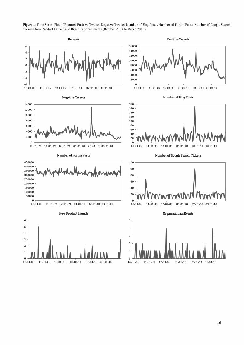
Figure 1 displays the graphs of the return and UGC data series and the series New Product Launch and

Organizational Events. The spikes in some of the graphs indicate two important dates for Apple. On

October 20th, 2009, the variable Returns reaches a maximum. On that same day there were 5 new

product launches: Apple unveiled the new iMac, the Magic Mouse and several updates on the MacBook.

The second important date is January 27th, 2010. On that day Steve Jobs introduced the iPad, during a

special product event. The number of positive tweets, negative tweets, blog posts and Google search

tickers reached a maximum on that day. The spikes in the series Organizational Events are related to

3 Gathering the data has been a time-consuming and intricate task, which is why we have a rather small sample. We hope to collect more data for future research, which will be discussed in chapter 6. 4 We understand that it is a rather unconventional approach to construct returns for Saturday and Sunday, but considering the fact that the dataset is small, omitting the UGC data in the weekends would make it too small to conduct our analysis. We recognize that other approaches would have been possible al well (such as aggregating the UGC data on weekends and Monday, although that would have made the sample smaller and would have caused an unnatural peak on Mondays), each coupled with pros and cons.

12

various mergers, client contracts, strategic alliances, lawsuits, reorganizations, corporate governance

changes, changes in key executives and labour relations. In the graphs of the Number of Blog Posts and

the Number of Google Search Tickers we can see a pattern; a seasonality. During weekends the

number of blog posts and Google search tickers is lower than during weekdays.5

Apart from the aberrant observations, another interesting feature to explore in the graphs of Returns

and the UGC variables of Figure 1 is heteroscedasticity. In the time series graphs of Returns, Positive

Tweets, Negative Tweets and Forum Posts the variance of the (deviations from the trend of the) time

series seems to change over time, which is a sign of heteroscedasticity. In the graphs of Blog Posts and

Google Search Tickers this somewhat difficult to see. In order to check whether some of the time series

exhibit time-varying volatility, we plotted time-varying estimates of the historical volatility, using a

rolling window of 10 days.6 Along with those estimates, we computed estimates of the exponentially-

weighted average of each of the squared variables, which gives more weight to more recent data.7 The

graphs are presented in Figure 1 in the Appendix. The time series Returns, Positive Tweets, Negative

Tweets and Forum Posts exhibit clear volatility clustering. The time series Blog Posts and Google

Search Tickers have volatility clustering as well, but the volatility in these time series does not appear

to be as time-varying as in the other four series.

Both squared returns and absolute returns are used as proxies for the volatility in returns. Similarly,

squaring the number of positive tweets, negative tweets, blog posts, forum posts or Google search

tickers can form proxies for the volatility of those series. We use those proxies to get some preliminary

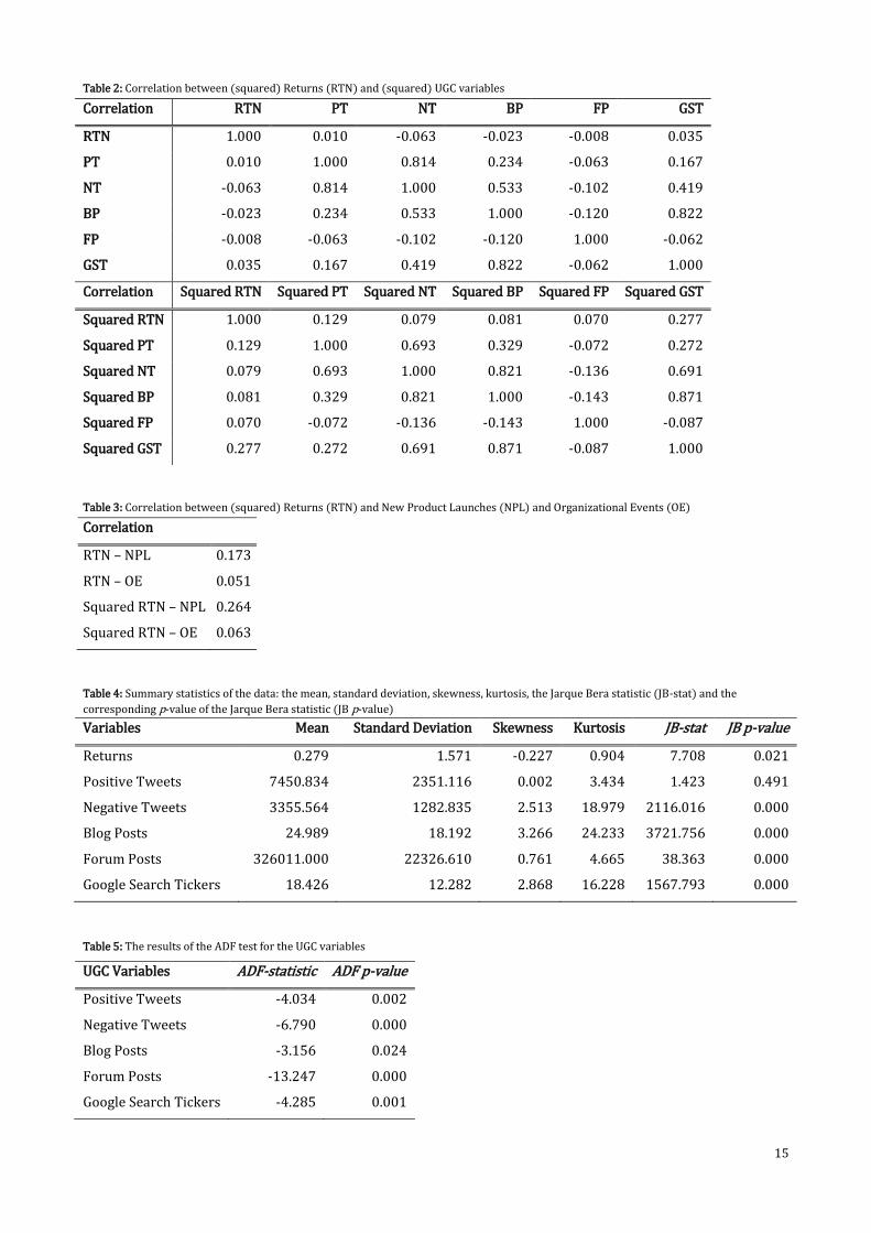
insights into the relationship between the variables. Table 2 shows the correlation between the

(squared) returns and (squared) UGC variables. The correlation between the UGC variables is bigger

than the correlation between the UGC variables and returns. The largest (negative) correlation

between returns and a UGC variable is between negative tweets and returns (-0.063), indicating a

negative relationship between these series: when returns increase, the volume of negative tweets

(slightly) decreases. The correlation between the squared variables (the volatility proxies) is in almost

all combinations larger than the correlation between the variables. The volatility of returns is

positively correlated with all volatilities of the UGC variables. The correlation between the volatility of

returns and the volatility of positive tweets (0.129) is quite large and so is the correlation between the

volatility of returns and the volatility of Google search tickers (0.277), indicating quite a strong

connection between the volatilities of returns and positive tweets and the volatilities of returns and

Google search tickers. Apart from studying the correlation between the (squared) variables estimated

over the entire sample, we plotted the correlation between (squared) returns and (squared) UGC

5 We will get back to that in the methodology in chapter 4. 6 With the chosen window width W of 10 days, this is ̂

∑ ( )

, where is the variable Returns, or one of the

UGC variables. 7 This volatility estimate is ̂

(1 ) ̂ ( ) , which is a weighted sum of last period’s volatility estimate and this

period’s squared variable ( ) and is the variable Returns, or one of the UGC variables. For we use 1/(1+(W/2)), with W being the window width of 10 days (Doan, 2013).

13

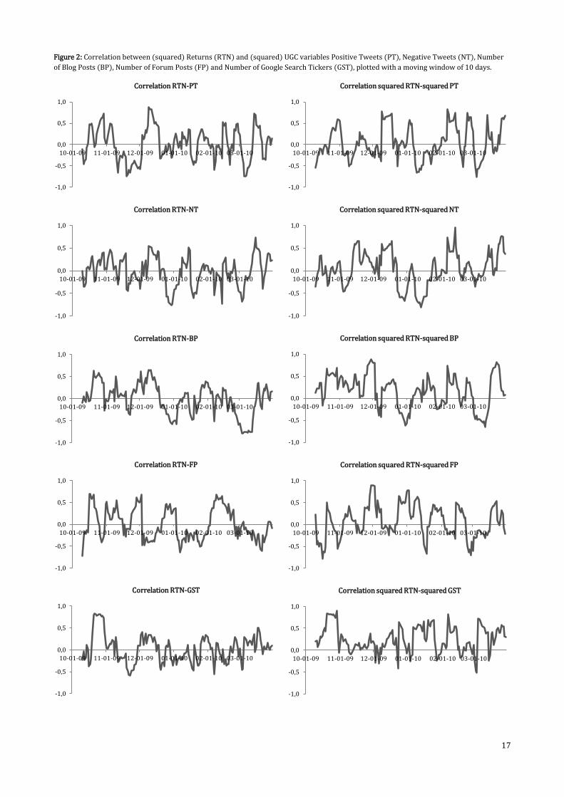
variables with a moving window of 10 days, displayed in Figure 2. These graphs show that the

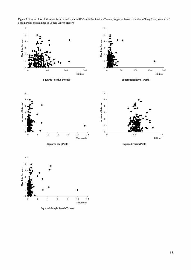
correlation between these variables and their volatility is time-varying. In order to give an impression

of the correlation using a different proxy, Figure 3 shows scatterplots of absolute returns with squared

UGC variables. The plots confirm the previous findings: the volatility of returns is correlated with the

volatility of positive tweets, blog posts, forum posts and Google search tickers. Finally, Table 3 shows

the correlation between (squared) returns and new product launches and organizational events.

Returns are more strongly correlated with new product launches than with organizational events and

the volatility in returns is even stronger correlated with new product launches.

Given the strong signs of volatility clustering and the time-varying nature of the correlation between

the (volatility) of the time series, we will investigate the relation between UGC variables and Returns

further using a multivariate GARCH BEKK model, as this takes these type of dynamics into account. A

multivariate GARCH model takes the time-varying nature of (co)variances into account and the BEKK

specification is especially suited for estimating possible spillover effects. We will explain this model in

more detail in the next chapter, but before proceeding to the methods, we present some summary

statistics of the variables in Table 4 and 5. The Jarque Bera statistics and corresponding p-values

indicate whether or not the series are normally distributed. For all series normality is rejected, except

for Positive Tweets. The skewness and kurtosis of Negative Tweets, Blog Posts and Google Search

Tickers are high, which is presumably caused by the spike in each of those series on January 27th, 2010

(the day the iPad was introduced). Hence, we will take the natural logarithm of those series before

estimating the multivariate GARCH BEKK model.8 In order to test the stationarity conditions the

Augmented Dickey-Fuller (ADF) test is applied to the UGC variables and the results are displayed in

Table 5. This unit root test is a statistical test to detect the presence of stationarity in time series used

in autoregressive models. If a time series is stationary, it means that the mean, variance and

covariance of this series remain unchanged by time shifts. If they are non-stationary, the mean and/or

the variance are time-varying. In that case we can study only a limited period and results are not

applicable to other periods. Moreover, the standard assumptions for asymptotic analysis are not valid

for non-stationary time series, indicating that hypothesis tests about regression parameters (t-tests

for instance) cannot be used in that case. The null hypothesis of the ADF-test states that there is a unit

root and the p-values in Table 5 show whether or not this null hypothesis can be rejected. All UGC

series are stationary.

We will now proceed with the methodology in the next chapter, taking the aforementioned findings

into account.

8 Since we have to match the scaling of the variables for our analysis (which will be explained in chapter 4), we will take the natural logarithm of Positive Tweets and Forum posts as well before estimating the BEKK model.

14

Table 1: Description of the variables

Variables Description Details about the variables

Returns Stock returns of

Apple

Stock return data of Apple

Positive Tweets Volume of positive

tweets about iPhone

e.g. I love the iPhone. Classified using a Support Vector Machine Algorithm.

Negative Tweets Volume of negative

tweets about iPhone

e.g. I hate the iPhone. Classified using a Support Vector Machine Algorithm.

Number of Blog

Posts

Number of posts by

influential bloggers

about iPhone

We collect the data for blogs about the brands from Newstex. Newstex’s

Authoritative Content feature enables us to select blogs from news organizations

and corporate blogs, as well as respected independent experts and thought

leader blogs, which include blogging sites such as Gawker.com, Mashable.com,

b5media.com, and consumerist.com.

Number of

Forum Posts

Number of posts by

users in internet

community forums

about iPhone

Discussion Forums are the number of posts on internet community forums that

mentioned the brand name in each day. An Internet community forum is an

online discussion site where people hold conversations in the form of posted

messages on topics that interest them. We collect the data for the discussion

forums from Google Groups.

Number of

Google Search

Tickers

Search volume for

AAPL in Google

Search Engine

Daily search volume for the ticker symbol “AAPL”. We obtain the daily search

volume from Google Trends (http://www.google.com/trends/) provided by

Google Search, which is the most popular search engine on the World Wide Web.

Google normalizes and scales the actual search volume of the keyword to remove

regional effects (Luo et al. 2013) and to hide the actual search volume of the

keyword in the Google search engine. The actual search volume is normalized by

Google using a common variable over a certain period, in this case it is the

maximum number of searches for the term “AAPL”. Since Google Trends does not

give daily number of searches for a period of more than 90 days we collected

daily searches from October to December 2009, November 2009 to January 2010,

December 2009 to February 2010, and January 2010 to March 2010. Hence, the

actual daily search volume is divided by the maximum search volume over a

period of 90 days. We mapped the common dates and synchronized the values

across these months to get the normalized values over our sample period. Since

the actual daily search volume is not available, we use this normalized daily

search volume as the variable Number of Google Search Tickers.

New Product

Launch

Number of new

product launches for

Apple

We measure new product announcements by the number of new product

launches made by the firm. We rely on the Capital IQ database for this particular

variable. We read each entry under the category of “Product-Related

Announcements” within the Key Developments feature of Capital IQ to ascertain

a new product launch.

Organizational

Events

Number of

organizational

related events for

Apple

We measure organizational events by counting and aggregating all key firm

events excluding new product announcements and financial events. We include

events such as mergers, client contracts, strategic alliances, lawsuits,

reorganizations, corporate governance changes, changes in key executives, and

labour relations. We obtain the data from Capital IQ’s key developments database

15

Table 2: Correlation between (squared) Returns (RTN) and (squared) UGC variables

Table 3: Correlation between (squared) Returns (RTN) and New Product Launches (NPL) and Organizational Events (OE)

Table 4: Summary statistics of the data: the mean, standard deviation, skewness, kurtosis, the Jarque Bera statistic (JB-stat) and the

corresponding p-value of the Jarque Bera statistic (JB p-value) Variables Mean Standard Deviation Skewness Kurtosis JB-stat JB p-value

Returns 0.279 1.571 -0.227 0.904 7.708 0.021

Positive Tweets 7450.834 2351.116 0.002 3.434 1.423 0.491

Negative Tweets 3355.564 1282.835 2.513 18.979 2116.016 0.000

Blog Posts 24.989 18.192 3.266 24.233 3721.756 0.000

Forum Posts 326011.000 22326.610 0.761 4.665 38.363 0.000

Google Search Tickers 18.426 12.282 2.868 16.228 1567.793 0.000

Table 5: The results of the ADF test for the UGC variables

Correlation RTN PT NT BP FP GST

RTN 1.000 0.010 -0.063 -0.023 -0.008 0.035

PT 0.010 1.000 0.814 0.234 -0.063 0.167

NT -0.063 0.814 1.000 0.533 -0.102 0.419

BP -0.023 0.234 0.533 1.000 -0.120 0.822

FP -0.008 -0.063 -0.102 -0.120 1.000 -0.062

GST 0.035 0.167 0.419 0.822 -0.062 1.000

Correlation Squared RTN Squared PT Squared NT Squared BP Squared FP Squared GST

Squared RTN 1.000 0.129 0.079 0.081 0.070 0.277

Squared PT 0.129 1.000 0.693 0.329 -0.072 0.272

Squared NT 0.079 0.693 1.000 0.821 -0.136 0.691

Squared BP 0.081 0.329 0.821 1.000 -0.143 0.871

Squared FP 0.070 -0.072 -0.136 -0.143 1.000 -0.087

Squared GST 0.277 0.272 0.691 0.871 -0.087 1.000

Correlation

RTN – NPL 0.173

RTN – OE 0.051

Squared RTN – NPL 0.264

Squared RTN – OE 0.063

UGC Variables ADF-statistic ADF p-value

Positive Tweets -4.034 0.002

Negative Tweets -6.790 0.000

Blog Posts -3.156 0.024

Forum Posts -13.247 0.000

Google Search Tickers -4.285 0.001

16

Figure 1: Time Series Plot of Returns, Positive Tweets, Negative Tweets, Number of Blog Posts, Number of Forum Posts, Number of Google Search

Tickers, New Product Launch and Organizational Events (October 2009 to March 2010)

0

2000

4000

6000

8000

10000

12000

14000

16000

10-01-09 11-01-09 12-01-09 01-01-10 02-01-10 03-01-10

Positive Tweets

-6

-4

-2

0

2

4

6

10-01-09 11-01-09 12-01-09 01-01-10 02-01-10 03-01-10

Returns

0

2000

4000

6000

8000

10000

12000

14000

10-01-09 11-01-09 12-01-09 01-01-10 02-01-10 03-01-10

Negative Tweets

0

20

40

60

80

100

120

140

160

180

10-01-09 11-01-09 12-01-09 01-01-10 02-01-10 03-01-10

Number of Blog Posts

0

50000

100000

150000

200000

250000

300000

350000

400000

450000

10-01-09 11-01-09 12-01-09 01-01-10 02-01-10 03-01-10

Number of Forum Posts

0

20

40

60

80

100

120

10-01-09 11-01-09 12-01-09 01-01-10 02-01-10 03-01-10

Number of Google Search Tickers

0

1

2

3

4

5

6

10-01-09 11-01-09 12-01-09 01-01-10 02-01-10 03-01-10

New Product Launch

0

1

2

3

4

5

10-01-09 11-01-09 12-01-09 01-01-10 02-01-10 03-01-10

Organizational Events

17

Figure 2: Correlation between (squared) Returns (RTN) and (squared) UGC variables Positive Tweets (PT), Negative Tweets (NT), Number

of Blog Posts (BP), Number of Forum Posts (FP) and Number of Google Search Tickers (GST), plotted with a moving window of 10 days.

-1,0

-0,5

0,0

0,5

1,0

10-01-09 11-01-09 12-01-09 01-01-10 02-01-10 03-01-10

Correlation RTN-PT

-1,0

-0,5

0,0

0,5

1,0

10-01-09 11-01-09 12-01-09 01-01-10 02-01-10 03-01-10

Correlation RTN-NT

-1,0

-0,5

0,0

0,5

1,0

10-01-09 11-01-09 12-01-09 01-01-10 02-01-10 03-01-10

Correlation RTN-BP

-1,0

-0,5

0,0

0,5

1,0

10-01-09 11-01-09 12-01-09 01-01-10 02-01-10 03-01-10

Correlation RTN-FP

-1,0

-0,5

0,0

0,5

1,0

10-01-09 11-01-09 12-01-09 01-01-10 02-01-10 03-01-10

Correlation RTN-GST

-1,0

-0,5

0,0

0,5

1,0

10-01-09 11-01-09 12-01-09 01-01-10 02-01-10 03-01-10

Correlation squared RTN-squared GST

-1,0

-0,5

0,0

0,5

1,0

10-01-09 11-01-09 12-01-09 01-01-10 02-01-10 03-01-10

Correlation squared RTN-squared FP

-1,0

-0,5

0,0

0,5

1,0

10-01-09 11-01-09 12-01-09 01-01-10 02-01-10 03-01-10

Correlation squared RTN-squared BP

-1,0

-0,5

0,0

0,5

1,0

10-01-09 11-01-09 12-01-09 01-01-10 02-01-10 03-01-10

Correlation squared RTN-squared NT

-1,0

-0,5

0,0

0,5

1,0

10-01-09 11-01-09 12-01-09 01-01-10 02-01-10 03-01-10

Correlation squared RTN-squared PT

18

Figure 3: Scatter plots of Absolute Returns and squared UGC variables Positive Tweets, Negative Tweets, Number of Blog Posts, Number of

Forum Posts and Number of Google Search Tickers.

0

1

2

3

4

5

6

0 100 200 300

Ab

solu

te R

etu

rns

Squared Positive Tweets

Millions

0

1

2

3

4

5

6

0 50 100 150 200

Ab

solu

te R

etu

rns

Squared Negative Tweets

Millions

0

1

2

3

4

5

6

0 5 10 15 20 25 30

Ab

solu

te R

etu

rns

Squared Blog Posts

Thousands

0

1

2

3

4

5

6

0 100 200

Ab

solu

te R

etu

rns

Squared Forum Posts

Billions

0

1

2

3

4

5

6

0 2 4 6 8 10 12

Ab

solu

te R

etu

rns

Squared Google Search Tickers

Thousands

19

4. Methods

To investigate the direct relation between stock returns and UGC we use a VAR(1) model. The

specification of the VAR(1) model9 is:

(1)

where and are n by 1 vectors at time t and t-1, respectively; n indicates the number of variables

included in the model. We will elaborate on the choice of variables in the next section. The vector

represents a n by 1 vector of constants and is a n by n matrix for parameters associated with the

lagged variables. The diagonal elements of the matrix , , measure the own lagged mean spillover

effects. The off-diagonal elements capture the cross mean spillover effects between the (lagged)

variables. The n by 1 vector of random error, , is the innovation for all n variables at time t and a

general multivariate GARCH model for this n-dimensional process ( , , ) is given by:

(2)

Where is a n-dimensional i.i.d. process with mean zero and covariance matrix equal to the identity

matrix . From these properties of and equation 2, it follows that [ | ] and

[ | ] , where represents the market information available at time t-1. To complete

the model, a parameterization for the n by n conditional variance-covariance matrix needs to be

specified ( ( , , , , , )) (Franses and Van Dijk, 2000). The parameterization

we choose is the multivariate GARCH BEKK model. With this type of multivariate GARCH model,

combined with the VAR(1) model, we investigate the relation between the variance of UGC metrics

and the variance of stock returns. The BEKK representation of the matrix is:

(3)

where and are n by n matrices and is a lower triangular matrix of constants. Engle and Kroner

(1995) refer to this formulation as the BEKK (Baba, Engle, Kraft and Kroner) representation. As the

second and third term on the right-hand-side of equation 3 are expressed as quadratic forms, is

guaranteed to be positive definite without the need for imposing constraints on the parameter

matrices and . The elements of the matrix measure the degree of lagged and cross innovation

(‘shocks’) from variable i to j. We refer to these effects as shock spillover effects. The diagonal

elements in matrix represent the ARCH effect (the effect of lagged shocks) and the off-diagonal

elements the cross-spillover effects. Negative coefficients in the off-diagonals of matrix mean that

the variance is affected more when the shocks move in opposite directions than when they move in the

same direction. The elements of the matrix measure the spillover of conditional volatility between

9 The lag length in the VAR model is determined using the Schwarz Information Criterion. We estimate the VAR model for 27 different combinations of variables (as listed in Table 6) and according to the SIC, all 27 combinations should have lag length 1 in the VAR model.

20

variable i and j. Hence, we refer to these effects as volatility spillover effects. The diagonal elements in

matrix measure the GARCH effect (the effect of lagged volatility) and the off-diagonal elements

measure the cross-volatility spillover effects. The guaranteed positive definiteness of and the fact

that all spillover effects are taken into account are the main advantages of the BEKK representation

opposed to other multivariate GARCH representations (Doan, 2013). This has contributed to our

decision to use the BEKK model, along with various drawbacks of other multivariate GARCH models.

Diagonal models such as the Diagonal BEKK and Diagonal VECH do not take spillovers into account

(matrices and are diagonal matrices), the full VECH model has more parameters than the BEKK

model and needs restrictions to guarantee positive definiteness, the common factors employed in

factor models (size, market-to-book, momentum) are not suitable for our dataset, the assumption of

constant correlation in the CCC model is too strict (considering the results of our preliminary analysis

in chapter 3) and the a drawback of the DCC model is the unrealistic assumption that all entries in the

conditional correlation matrix are influenced by the same coefficients. Although some of these

alternative models have some advantages over the BEKK model (some have fewer parameters), their

disadvantages led us to favour the BEKK representation over the other models.

The aforementioned n variables are a combination of the UGC variables Positive Tweets, Negative

Tweets, Number of Blog Posts, Number of Forum Posts and Number of Google Search Tickers and the

variable Returns. The values of the coefficients of matrices and in the BEKK representation are

sensitive to the scales of these variables, since there is no standardization to a common variance. This

causes (relatively) higher variance series to have higher off-diagonal coefficients than lower variance

series. Rescaling a variable keeps the diagonals of and the same, but forces a change in the scale of

the off-diagonals (Doan, 2013). Figure 1 shows that there is a wide variety in the scaling of the series.

In order to match the scaling we take the natural logarithm10 of the UGC series Positive Tweets,

Negative Tweets, Number of Blog Posts, Number of Forum Posts and Number of Google Search Tickers.

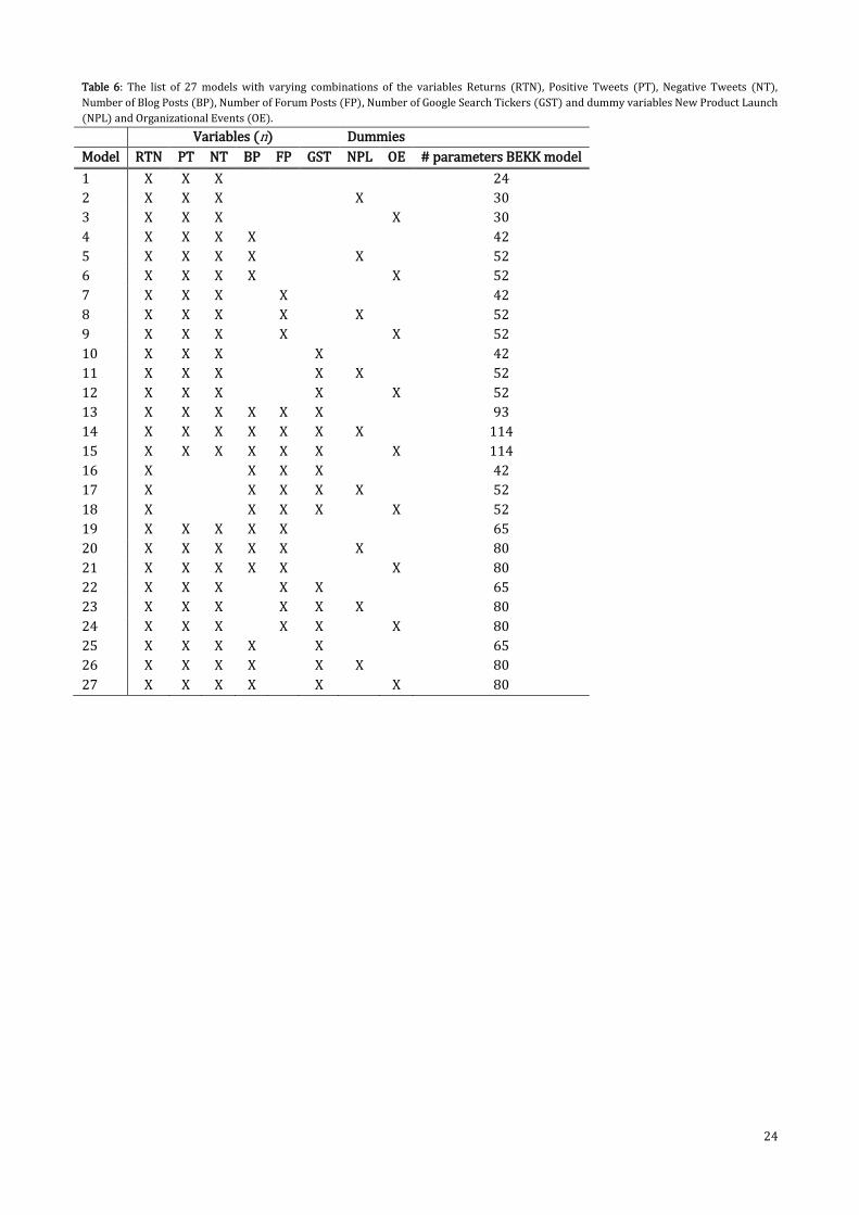
We perform a ‘meta-analysis’11 to study the shock and volatility spillover effects between UGC

variables and Returns by estimating 27 multivariate GARCH BEKK models using various combinations

of variables. Table 6 displays those 27 combinations. Since the total number of parameters in the

GARCH BEKK equation differs depending on the number of variables included in the model, we also

list the total number of parameters per model in Table 6. Certain shock and volatility spillover effects

are estimated in all or a part of the 27 models and we compute the average of those effects. The

purpose of estimating these different BEKK models is not just to average and generalize the results, it

is also to investigate interesting combinations of variables. Since the BEKK model might suffer from

10 Although in general taking the natural logarithm does not guarantee that the scaling of the variables is matched, it is sufficient for our dataset. We are aware of other options (e.g. subtracting the mean and then dividing by the unconditional sample standard deviation), but the advantage of the natural logarithm is that coefficients on the natural logarithm scale remain directly interpretable, which we prefer over advantages of other options. 11 The term meta-analysis is usually used to indicate combined results from different studies. In this case not different studies, but different models are combined. The term is therefore mainly used out of convenience opposed to alternatives as ‘an analysis of the summarized results of 27 models with various combinations of variables’.

21

the so-called ‘curse of dimensionality’ and our dataset is rather small, we decided to estimate the

model for different combinations of time series. The possible consequences of this curse of

dimensionality are not clear beforehand and could vary from overfitting to numerical instabilities.

Hence, including all variables might not guarantee a ‘better’ model opposed to a smaller version

(Verleysen et al., 2005), which is why we choose to model different combinations of variables.12 To be

able to discuss and compare all these results (reviewing whether effects are large/ small or

significant/insignificant in most models), we summarized them and refer to this as a ‘meta-analysis’.13

Table 6 also shows that we add a dummy variable to the BEKK equation in some of these models. The

dummy variables are Dummy New Product Launch and Dummy Organizational Events and they are

computed using the series New Product Launch and Organizational Events and they are used to study

the possible influence of these launches or events on the (co)variances of returns and UGC variables. If

one or more new product launches occur on a specific date in the series New Product Launch, the

variable Dummy New Product Launch lists a 1 on that date, and if there are no launches a 0 is listed.

The same procedure is used to compute the variable Dummy Organizational Events, where a 1

indicates one or more organizational events on a certain date and 0 indicates no events on that date.

Adding one of these dummies to the BEKK equation adjusts the term. Due to the fact that there are

sign restrictions in the BEKK recursion because of the desire to enforce positive-definiteness, adding a

dummy in the recursion comes down to replacing with:

( ) ( ) (4)

Where is, like , a lower triangular matrix. Adding the dummy, , this way enforces positive

definiteness and guarantees that the model is not sensitive to the choice of representation of the

dummy, due to the fact that adjustments to matrix are made before squaring. In chapter 2 we

described the seasonality present in the number of blog posts and the number of Google search tickers.

This could be taken into account by creating a dummy, but that would increase the number of

parameters in each model and considering the large number of parameters we have in the BEKK

recursions (see Table 6), we decided not to create a dummy for the weekends as well. As it might be a

possibility to explore in future research, we get back to that in the discussion in chapter 5.

The mean equation 1 and the BEKK equation 3 (or the BEKK equation 3 with replaced by equation

4) are estimated simultaneously by the BFGS maximum likelihood method. The BFGS (Broyden,

Fletcher, Goldfarb and Shanno) method is used to solve the nonlinear optimization problem and to

produce the maximum likelihood parameter estimates and their corresponding asymptotic standard

errors. BFGS estimates the curvature (and therefore the covariance matrix of the parameter estimates)

12 This approach is rather unconventional opposed to other studies using multivariate GARCH models, where usually one model is chosen and presented. Due to our small dataset we preferred estimating BEKK models using multiple combinations of variables over choosing one model with the risk of that one model suffering from overfitting or numerical instabilities. 13 We understand that merely providing these summarized results might not be the ideal approach to discussing results of a multivariate GARCH BEKK model, which is why we will discuss one model separately.

22

using an update method which will give a different answer for different initial guess values. A pre-

estimation ‘simplex’ procedure is used with approximately 20 iterations before proceeding to the

BFGS method. If we start the estimation with the BFGS method, the estimate of the curvature using the

guess values can lead to inaccurate moves in the early iterations. Starting the estimation with a pre-

estimation simplex procedure before proceeding to the BFGS method eliminates that problem. The

first iterations using the simplex procedure move the parameter set off the guess values into what is

likely to be the right direction. The BFGS method uses those values as initial values instead of the guess

values for doing the final estimates (Doan, 2013). In order to correct for possible misspecification we

compute Bollerslev-Wooldridge standard errors in this final estimation.

The fit of the BEKK model is exactly the same if you change the sign of the entire or matrix, as the

model is not globally identified. This means that the sign of the coefficients should be interpreted with

caution, although in most cases the sign will be steered in the right direction by the initial guess values

(Doan, 2013).

To test the adequacy of the models we perform a multivariate ARCH test on the residuals of the BEKK

recursion, to check the possible presence of remaining arch effects.

Impulse response functions describe the dynamics of a VAR model. To describe the dynamics of a

multivariate GARCH BEKK model, we use a similar model: a volatility impulse response function

(hereafter: VIRF) (Hafner and Herwartz, 2006). With IRFs, the impulses are responses to a

standardized set of shocks, which can be rescaled to get responses to any other set of shocks. These

type of shocks are not possible in VIRFs, as the enters as a square in the recursion. The standardized

shocks may therefore be out of scale, so we need to calculate the VIRFs as the responses to a complete

vector of shocks (Doan, 2013). The shocks we include in the recursion are characteristic for the data

(Hafner and Herwartz, 2006). We choose to use two important dates for Apple: the October 20th, 2009

and January 27th, 2010. As explained in chapter 3: on October 20th, 2009, the variable Returns reaches

a maximum and on that day 5 new products were launched. On January 27th, 2010 Steve Jobs launched

the iPad and the number of positive tweets, negative tweets, blog posts and Google search tickers

reached a maximum. To compute the VIRF, we need to convert the BEKK estimates into VECH

estimates (Doan, 2013). The BEKK model is a restriction of the VECH model. A VECH(1,1) model is

written as:

( ) ( ) ( ) (5)

The vech operator converts a n by n symmetric matrix into a n(n + 1)/2 vector by eliminating the

duplicated entries. and are full (n(n + 1)/2 x n(n + 1)/2) matrices and is a n(n + 1)/2 x 1

vector which is the vech of a positive semi-definite matrix. The VECH model is rarely used, because it

contains a very large number of free parameters. Even though it is not very useful for estimation, it is

23

useful for forecasting and similar calculations, such as computing a VIRF (Doan, 2013). Forecasts of

recursion 5 can be generated via:

( ̂ ) ( ) ( )

( ̂ ) ( ) ( ̂ ) (6)

To create shocks for the VIRF we pick either and transform to or pick

directly (Doan,

2013). Computing volatility forecasts with a shock (with 0) is different compared to equation 6:

( ) ( )

( ) ( ) ( )

(7)

Hafner and Herwartz (2006) refer to this function of the model coefficients and the shock (not the

data) as the conditional volatility profile. In the standard IRF, we compute the revision in the forecast

by observing the given shock. For the analogous idea in the volatility equation, we use a formula

similar to equation 7 for the VIRF, with a slightly different input (Doan, 2013):

( ) ( )

( ) ( ) ( )

(8)

Where is the variance-covariance matrix for time t. The VIRF depends upon the data now through

– the ‘shock’ to the variance is the amount by which the exceeds its expected value (Doan,

2013). As with other types of impulse responses, constants ( ) drop out, because it is the difference

in the behaviour with and without the added shocks that matters. In the VIRFs and conditional

volatility profiles we estimate we take k=10 days.

All of the above is programmed using the software of WinRATS, which is suitable for computing

multivariate GARCH models, especially the BEKK specification (Brooks, Burke and Persand, 2003).

24

Table 6: The list of 27 models with varying combinations of the variables Returns (RTN), Positive Tweets (PT), Negative Tweets (NT),

Number of Blog Posts (BP), Number of Forum Posts (FP), Number of Google Search Tickers (GST) and dummy variables New Product Launch

(NPL) and Organizational Events (OE).

Variables (n) Dummies

Model RTN PT NT BP FP GST NPL OE # parameters BEKK model

1 X X X 24

2 X X X X 30

3 X X X X 30

4 X X X X 42

5 X X X X X 52

6 X X X X X 52

7 X X X X 42

8 X X X X X 52

9 X X X X X 52

10 X X X X 42

11 X X X X X 52

12 X X X X X 52

13 X X X X X X 93

14 X X X X X X X 114

15 X X X X X X X 114

16 X X X X 42

17 X X X X X 52

18 X X X X X 52

19 X X X X X 65

20 X X X X X X 80

21 X X X X X X 80

22 X X X X X 65

23 X X X X X X 80

24 X X X X X X 80

25 X X X X X 65

26 X X X X X X 80

27 X X X X X X 80

25

5. Results

In this chapter we report the results of mean, shock and volatility spillover effects estimated over 27

different models. Table 1 in the appendix displays the estimated results per model and in this chapter

we report the meta-analysis of those 27 models. Certain mean, shock and volatility spillover effects are

estimated in a selection of the 27 models (see Table 6, where the variables included in each model are

listed) and we study the overall effect by computing averages. For instance, spillover effects between

Returns and Positive Tweets are estimated in 24 models, (1-15 and 19-27) so we compute the average

mean, shock and spillover effects over these 24 models. The coefficients that represent a spillover

effect can either be significant or insignificant, depending on whether their p-value is below 10

percent. For each (average) spillover effect we report the ‘percentage significant’, expressing the

significant estimated coefficients as a percentage of the total estimates of the spillover effect. We

discuss one model separately, to give an indication of how each model individually should be

discussed opposed to the summarized results. Furthermore, we discuss the volatility impulse response

functions.

5.1 Mean Spillover Effects

Table 7 shows the average mean spillover effects estimated over all 27 models. The matrix Γ in the

mean equation, with parameters γij captures the relationship between Returns (RTN), Positive Tweets

(PT), Negative Tweets (NT), Number of Blog Posts (BP), Number of Forum Posts (FP) and Number of

Google Search Tickers (GST). For example, γ13 represents the mean spillover effect from Negative

Tweets on Returns. The average of all coefficients, the average of all significant coefficients

(coefficients with a p-value below 10 percent) and the average of all coefficients in absolute numbers

are calculated, including the percentage of the coefficients that turn out to be significant. For example,

Table 7 shows that γ13 corresponds to a percentage of 41.67, indicating that the effect, which was

estimated in 24 models, was significant in 41.67 percent of the 24 estimates. We focus the discussion

of our results on effects that are significant in at least 50 percent of the estimates and on the

magnitude, sign and meaning of the effects.

Table 7 displays high percentages for the diagonal parameters γ11, γ22, γ33, γ44 and γ66, which means

that Returns, Positive Tweets, Negative Tweets, Blog Posts and Google Search Tickers (positively)

depend on their first lag in 100, 100, 100, 100 and 80 percent of the estimates.

The mean spillovers between the UGC variables and returns are represented by the off-diagonal

parameters γij. The off-diagonal parameters γ26 and γ62, γ34 and γ43, γ36 and γ63 are all statistically

significant (p-values below 10 percent) in at least 50 per cent of the estimates, indicating that there

are bidirectional spillovers from Google search tickers to Positive Tweets, from Blog Posts to Negative

Tweets and from Google Search Tickers to Negative Tweets, respectively. The bidirectional spillovers

26

between the number of Google search tickers and positive tweets (γ26 and γ62) are negative, implying

that the past number of Google search tickers decreases the future volume of negative tweets and that

the past volume of negative tweets decreases the future number of Google search tickers. The effect

from the number of blog posts on the volume of negative tweets is small and negative (γ34), whereas

the counterpart (γ43) is larger and positive. Hence, the past number of blog posts slightly decreases the

future volume of negative tweets whereas the past volume of negative tweets slightly increases the

future number of blog posts.

The off-diagonal parameters γ32, γ42, γ45 and γ46 are statistically significant (p-values below 10 percent)

in more than 50 percent of the estimates, whereas their counterparts are not, indicating that there are

unidirectional linkages from the volume of positive tweets to negative tweets (which is a positive

spillover) and from the volume of positive tweets, the number of forum posts and the number of

Google search tickers to the number of blog posts (all three are negative spillovers).

The results of the mean spillover effects indicate a strong connection between the various UGC

metrics, whereas the link between returns and the UGC metrics is much weaker. The next subsection

proceeds with studying the relationship between returns and UGC variables in terms of shock and

spillover effects.

5.2 Shock and volatility spillover effects

Table 8 displays the average shock spillover effects between Returns (RTN), Positive Tweets (PT),

Negative Tweets (NT), Number of Blog Posts (BP), Number of Forum Posts (FP) and Number of Google

Search Tickers (GST). For example, ‘PT(-1) -> RTN’ indicates the shock spillover effects from the

volume of positive tweets to returns. ‘Average coefficients’ refers to the average shock spillover effect

as measured over all the models in which this effect is estimated, ‘Average significant coefficients’ is

the average of the significant shock spillover effects and ‘Average absolute coefficients’ is the average

of all the spillover effects expressed in absolute values. The column ‘Percentage significant’ displays

the percentage of the estimated coefficients that are significant (have a p-value below 10 percent). For

example, the percentage 51.85 in the first row of Table 8 indicates that of the 27 models in which this

effect was estimated, 51.85 percent of the effects are statistically significant (p-value < 0.10). Table 9

displays the results on volatility spillover effects in a similar way as the shock spillover effects

presented in Table 8. The discussion of the results is focussed on spillover effects that are significant in

at least 50 percent of the estimates and on the sign and magnitude and meaning of the effects.

The ARCH effects (the effect of lagged shocks) are captured by the diagonal elements of the matrix

and the GARCH effects (the effect of past volatility) are captured by the diagonal elements of the

matrix of the multivariate GARCH BEKK model. Table 8 shows that the average ARCH effect is

significant in more than 50 percent of the estimates for Returns, Negative Tweets, Forum Posts and

27

Google Search Tickers, implying presence of ARCH effects in those three UGC variables and the stock

returns of Apple. The magnitude of the ARCH effect is highest for Negative Tweets (0.376), followed by

Forum Posts (-0.230). Table 9 shows that the average GARCH effect is significant in more than 50

percent of the estimates for Returns, Negative Tweets and Forum Posts, implying that own past

volatility largely affects the conditional variance of those series. The magnitude of the GARCH effect is

highest for Negative Tweets (0.697), followed by Forum Posts (0.628).

The off-diagonal elements of matrices and capture the cross-linkages, such as shock spillover and

volatility spillover, among UGC variables and returns. Table 8 shows evidence of bidirectional shock

spillovers (shock transmissions) between the number of Google search tickers and the volume of

positive tweets and the number of Google search tickers and the volume of negative tweets, which

indicates a strong connection between these UGC metrics. Past shocks in the volume of positive tweets

decrease the future volatility in the number of Google search tickers and past shocks in the number of

Google search tickers decrease the future volatility in the volume of positive tweets, although the

magnitude of both effects is small. Past shocks in the number of Google search tickers slightly decrease

the volatility in the volume of negative tweets and shocks in the volume of negative tweets increase

the volatility in the number of Google search tickers.

Table 8 also shows evidence of unidirectional shock spillovers from Blog Posts to Returns, from

Negative Tweets to Positive Tweets, from Returns to Negative Tweets, from Blog Posts to Negative

Tweets and from Google search tickers to Blog Posts. Past shocks in the number of blog posts decrease

volatility in returns. The number of blog posts is the only UGC metric with a significant (negative)

shock spillover effect on stock returns in at least 50 percent of the estimates. For investors this could

mean that by reviewing the presence of shocks in the number of blog posts an increase in the volatility

of stock returns could be anticipated, which in turn could be used for hedging or portfolio strategies.

The volume of negative tweets is the only UGC metric whose volatility is (positively) affected by past

shocks in stock returns in at least 50 percent of the estimates, but the effect is small. The remaining

unidirectional shock spillovers indicate that shocks in the volume of negative tweets increase the

future volatility in the volume of positive tweets, that shocks in the number of blog posts decrease the

future volatility of the volume of negative tweets and that shocks in the number of Google search

tickers increase the future volatility of the number of blog posts.

Table 9 shows no evidence of bidirectional volatility spillover effects, merely of unidirectional effects.

Past volatility in the number of Google search tickers decreases the future volatility of the volume of

positive tweets, the volume of negative tweets and the number of blog posts. Past volatility in the

number of blog posts decreases the future volatility in the volume of negative tweets. The future

volatility of the number of forum posts decreases due to past volatility in the volume of positive tweets

decreases and it increases due to past volatility in the volume of negative tweets. The only UGC metric

of which the future volatility is affected by past volatility in stock returns (among the effects that are

28

significant in at least 50 percent of the estimates) is the number of Google search tickers, but the

magnitude is small (0.044), indicating a weak integration between the time series.

Figures 4 and 6 display the plots of the (significant) shock spillover effects between the variables, of

which the average values are presented in Table 8. Figures 5 and 7 display plots of the (significant)

volatility spillover effects, corresponding to the averages in Table 9. The plots show that the effects can

vary widely between models, both in magnitude and in sign. As mentioned in the methodology section:

the fit of the BEKK model is exactly the same if you change the sign of the entire or matrix, as the

model is not globally identified. This means that the sign of the coefficients should be interpreted with

caution, although in most cases the sign will be steered in the right direction by the initial guess values

(Doan, 2013). The plots show that the sign of an effect is the same in most cases, but sometimes it

differs.

The multivariate ARCH test is used to test for any remaining arch effects and the results are displayed

in Table 10. If the p-value indicates no significance (value above 10 percent), there is no remaining

series dependence in the residuals of that model. In 13 of the 27 models the test statistics are

insignificant, indicating the appropriateness of the fitted variance-covariance equations by the

multivariate GARCH BEKK model.

Some of the models contain a dummy variable in the GARCH BEKK recursion, either the dummy New

Product Launch, or Organizational Events. As displayed in equation 4, adding a dummy adds

coefficients to the coefficients. Coefficient is the variance intercept, and all the other

coefficients are factors of that variance intercept (Doan, 2013). This means that the coefficients do not

have simple interpretations, opposed to the coefficients in the and matrices. The coefficients,

which are added to the coefficients, are therefore not easy to interpret either. However, what we can

see from the results of the multivariate ARCH tests is that adding a dummy can lead to a better fit of

the multivariate GARCH BEKK model. Some of the models had remaining series dependence when

there was no dummy in the BEKK model, but when a dummy was added, the ARCH test showed no

proof of remaining series dependence, indicating that adding that dummy had led to a better fit. This

was the case for model 5 (opposed to model 4 without a dummy), models 11 and 12 (opposed to

model 10 without a dummy) and models 23 and 24 (opposed to model 22 without a dummy).

In the next subsection we discuss the results of one of the 27 models separately.

5.3 Discussion of one model

To give an impression of how each of the 27 results of the BEKK models should be discussed

individually we describe the results of one model, number 5. This model contains the variables

Returns, Positive Tweets, Negative Tweets and Blog Posts. The results are listed in the appendix in

Table 1, model 5. As the diagonal elements γ11, γ22, γ33 and γ44 are statistically significant with p-values

29

below 5 percent, all four variables depend on their first lag. The values of past returns, volume of

positive tweets, volume of negative tweets and number of blog posts positively affect the values of the

returns, the volume of positive and negative tweets and the number of blog posts the following day.

The cross-linkages are represented by the off-diagonal elements, of which γ32, γ42 and γ43 are

statistically significant. The past volume of positive tweets increases the future volume of negative

tweets and decreases the future number of blog posts. The past volume of negative tweets on the other

hand increases the future number of blog posts. The difference in influence of the volume of positive

and negative tweets on the number of blog posts might be due to the negativity bias. As people are

more inclined to respond to (and believe) negative news, they might pay more attention to it, resulting

in more blog posts. The link between positive and negative tweets is probably due to the fact that

topics on Twitter are indicated with a hashtag (e.g. ‘#iPhone’), which makes it likely that the number

of positive and negative tweets regarding the same subject, in this case the iPhone, move closely

together.

The diagonal elements of the matrix show that there are statistically significant (at a 5 percent level)

ARCH effects in the volume of negative tweets and the number of blog posts, implying that own past

shocks largely affect the conditional variance of these two series. The conditional variance of negative

tweets decreases due to own past shocks and the conditional variance of the number of blog posts

increases due to own past shocks. The off-diagonal elements of the matrix show that there are

unidirectional shock spillover effects between some of the UGC variables. Past shocks in positive

tweets increase the future volatility of the number of blog posts, whereas past shocks in negative

tweets decrease the future volatility of the number of blog posts. The size of these two shock spillovers

is similar (around 1.5). Furthermore, past shocks in the volume of negative tweets decreases future

volatility in the volume of positive tweets.

The diagonal elements of the matrix show that the returns have a significant GARCH effect,

indicating that the volatility in returns is negatively affected by own past volatility. The off-diagonal

elements capture some statistically significant volatility spillovers. Past volatility in the volume

positive tweets increases the future volatility in the volume of negative tweets, whereas past volatility

in the number of blog posts decreases the future volatility in the volume of negative tweets. Past

volatility in the volume of negative tweets increases future volatility in the stock returns and this effect

is the largest volatility spillover effect in this model (3.009). This means that investors can anticipate a

possible future increase in the volatility of the Apple stock by studying the volatility in negative tweets.

The dummy New Product Launches is added to the model and some of the elements of the matrix

are statistically significant. As mentioned earlier, the constant and dummies are difficult to interpret.

However, what we can see if we compare the multivariate ARCH test results in Table 10 of model 5

with model 4, is that adding this dummy enhances the fit of the multivariate GARCH BEKK model. The

30

results of the multivariate ARCH test indicate the appropriateness of the fitted variance-covariance

equation by the multivariate GARCH BEKK model.

5.4 Volatility Impulse Response Functions

Figure 8 displays the volatility impulse response functions (VIRFs) and conditional volatility profiles

for model 1 containing the three variables Returns, Positive Tweets and Negative Tweets. This means

that the VIRFs and conditional volatility profiles are plotted for 6 (co)variances: the variance of

Returns, the covariance between Returns and Positive Tweets, the variance of Positive Tweets, the

covariance between Returns and Negative Tweets, the covariance between Positive Tweets and

Negative Tweets and the variance of Negative Tweets. The two historical shocks which we used to

compute the VIRFs and conditional volatility profiles are characteristic for our data: October 20th,

2009, when 5 new products were launched, and January 27th, 2010, when Steve Jobs first introduced

the iPad. Both of these dates concern new products of Apple, but on January 27th the product was

introduced via a big keynote speech and was not made available to the public yet, whereas on October

20th the introductions were done via smaller press releases and most of the products were instantly

available to the public.

The left column shows that the variance of Returns displays the biggest positive shock, the other

shocks in that column are closer to zero or negative. The impulse response in the covariance between

Returns and Positive Tweets is smaller and positive as well. The other four impulse responses in the

column are all negative, slowly moving to zero. The conditional volatility profiles of the variance of

Returns, the covariance of Returns and Positive Tweets and the covariance of Returns and Negative

Tweets are close to the corresponding impulse responses. The conditional volatility profiles are just

slightly above the impulse responses, which can be explained by the way these functions were

constructed (see equations 7 and 8 in chapter 3). The conditional volatility profile is a function of the

model coefficients and the shock (the baseline is set to zero), whereas the VIRF depends upon the data

as well through the variance-covariance matrix. A shock in the VIRF is the amount by which it exceeds

the expected value. Hence, the conditional volatility profile and the VIRF have a positive difference if

the expected value is close to the shock (in that case the VIRF is close to zero and the corresponding

conditional volatility profile is positive) (Hafner and Herwartz, 2006). This is visible in the three

remaining plots of the left column: the conditional volatility profiles indeed have positive values, are

located above the VIRFs and the VIRFs are negative. In these plots the conditional volatility profiles

could lead to the misbelief that the effect of the shock on the (co)variance of (between) Positive and

Negative Tweets is positive, while it is not given the data.

The right column in Figure 8 shows that the shocks are strongly positive in the variances of Positive

Tweets, Negative Tweets, and that effect appears in the 3 covariances as well. The conditional

volatility profiles are all just slightly above the impulse responses, indicating that the shocks differ

31

from the expected value. The difference in the effects in the two columns indicates that the

announcement of the iPad had a much bigger effect than the launch of the 5 new products. Even

though most of those 5 products were instantly available, those 5 product launches led to smaller

shocks than the introduction of the iPad. This could imply that those products were perhaps not as

innovative as the iPad, leading to smaller responses in stock returns and the volume of tweets. Hence,

new product launches can cause shocks in volatilities of UGC and stock returns, but the magnitude of

the impact depends on the product being launched.

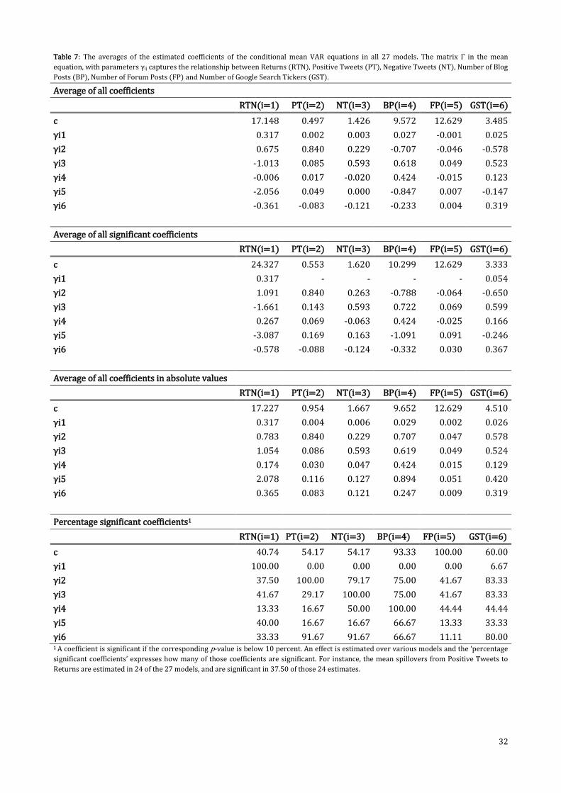
32

Table 7: The averages of the estimated coefficients of the conditional mean VAR equations in all 27 models. The matrix Γ in the mean

equation, with parameters γij captures the relationship between Returns (RTN), Positive Tweets (PT), Negative Tweets (NT), Number of Blog

Posts (BP), Number of Forum Posts (FP) and Number of Google Search Tickers (GST).

Average of all coefficients

RTN(i=1) PT(i=2) NT(i=3) BP(i=4) FP(i=5) GST(i=6)

c 17.148 0.497 1.426 9.572 12.629 3.485

γi1 0.317 0.002 0.003 0.027 -0.001 0.025

γi2 0.675 0.840 0.229 -0.707 -0.046 -0.578

γi3 -1.013 0.085 0.593 0.618 0.049 0.523

γi4 -0.006 0.017 -0.020 0.424 -0.015 0.123

γi5 -2.056 0.049 0.000 -0.847 0.007 -0.147

γi6 -0.361 -0.083 -0.121 -0.233 0.004 0.319

Average of all significant coefficients

RTN(i=1) PT(i=2) NT(i=3) BP(i=4) FP(i=5) GST(i=6)

c 24.327 0.553 1.620 10.299 12.629 3.333

γi1 0.317 - - - - 0.054

γi2 1.091 0.840 0.263 -0.788 -0.064 -0.650

γi3 -1.661 0.143 0.593 0.722 0.069 0.599

γi4 0.267 0.069 -0.063 0.424 -0.025 0.166

γi5 -3.087 0.169 0.163 -1.091 0.091 -0.246

γi6 -0.578 -0.088 -0.124 -0.332 0.030 0.367

Average of all coefficients in absolute values

RTN(i=1) PT(i=2) NT(i=3) BP(i=4) FP(i=5) GST(i=6)

c 17.227 0.954 1.667 9.652 12.629 4.510

γi1 0.317 0.004 0.006 0.029 0.002 0.026

γi2 0.783 0.840 0.229 0.707 0.047 0.578

γi3 1.054 0.086 0.593 0.619 0.049 0.524

γi4 0.174 0.030 0.047 0.424 0.015 0.129

γi5 2.078 0.116 0.127 0.894 0.051 0.420

γi6 0.365 0.083 0.121 0.247 0.009 0.319

Percentage significant coefficients1

RTN(i=1) PT(i=2) NT(i=3) BP(i=4) FP(i=5) GST(i=6)

c 40.74 54.17 54.17 93.33 100.00 60.00

γi1 100.00 0.00 0.00 0.00 0.00 6.67

γi2 37.50 100.00 79.17 75.00 41.67 83.33

γi3 41.67 29.17 100.00 75.00 41.67 83.33

γi4 13.33 16.67 50.00 100.00 44.44 44.44

γi5 40.00 16.67 16.67 66.67 13.33 33.33

γi6 33.33 91.67 91.67 66.67 11.11 80.00 1 A coefficient is significant if the corresponding p-value is below 10 percent. An effect is estimated over various models and the ‘percentage

significant coefficients’ expresses how many of those coefficients are significant. For instance, the mean spillovers from Positive Tweets to

Returns are estimated in 24 of the 27 models, and are significant in 37.50 of those 24 estimates.

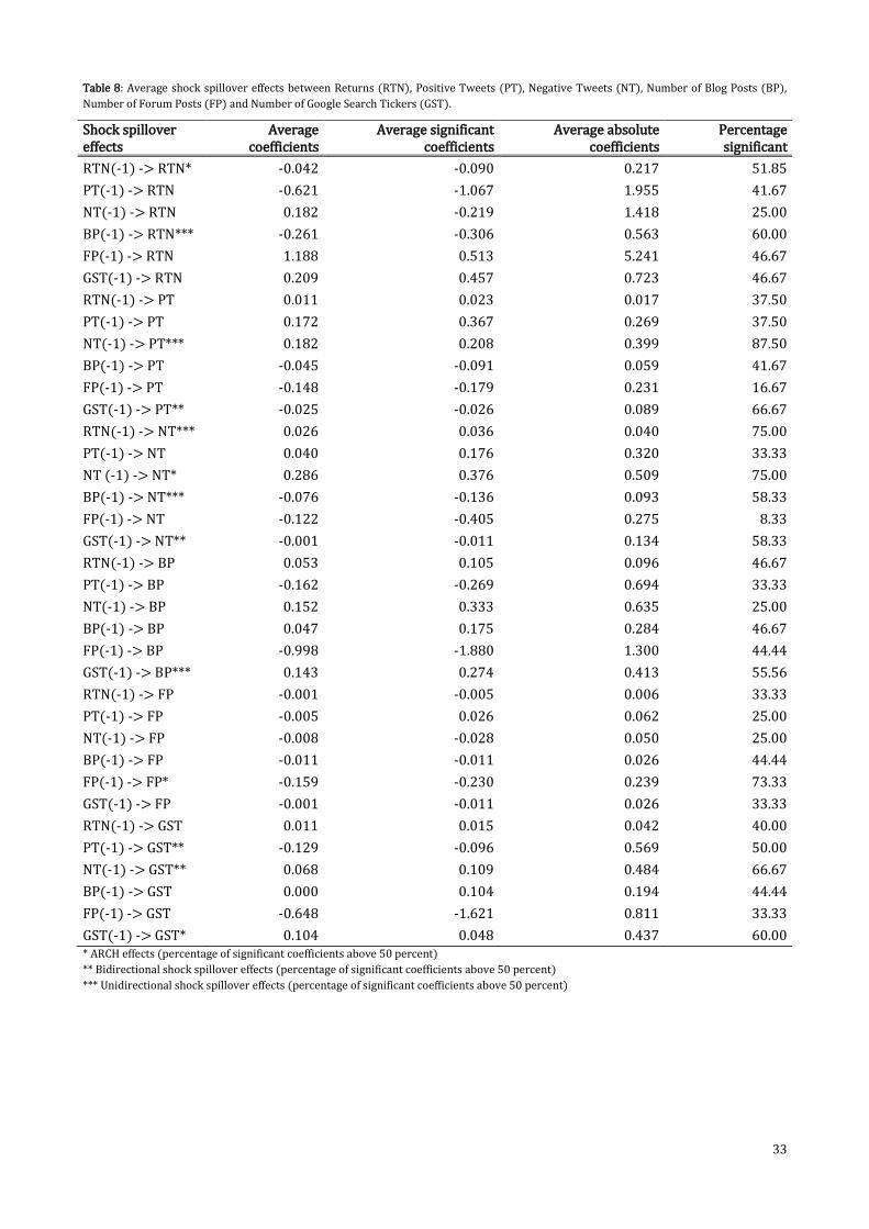
33

Table 8: Average shock spillover effects between Returns (RTN), Positive Tweets (PT), Negative Tweets (NT), Number of Blog Posts (BP),

Number of Forum Posts (FP) and Number of Google Search Tickers (GST).

* ARCH effects (percentage of significant coefficients above 50 percent)

** Bidirectional shock spillover effects (percentage of significant coefficients above 50 percent)

*** Unidirectional shock spillover effects (percentage of significant coefficients above 50 percent)

Shock spillover effects

Average coefficients

Average significant coefficients

Average absolute coefficients

Percentage significant

RTN(-1) -> RTN* -0.042 -0.090 0.217 51.85

PT(-1) -> RTN -0.621 -1.067 1.955 41.67

NT(-1) -> RTN 0.182 -0.219 1.418 25.00

BP(-1) -> RTN*** -0.261 -0.306 0.563 60.00

FP(-1) -> RTN 1.188 0.513 5.241 46.67

GST(-1) -> RTN 0.209 0.457 0.723 46.67

RTN(-1) -> PT 0.011 0.023 0.017 37.50

PT(-1) -> PT 0.172 0.367 0.269 37.50

NT(-1) -> PT*** 0.182 0.208 0.399 87.50

BP(-1) -> PT -0.045 -0.091 0.059 41.67

FP(-1) -> PT -0.148 -0.179 0.231 16.67

GST(-1) -> PT** -0.025 -0.026 0.089 66.67

RTN(-1) -> NT*** 0.026 0.036 0.040 75.00

PT(-1) -> NT 0.040 0.176 0.320 33.33

NT (-1) -> NT* 0.286 0.376 0.509 75.00

BP(-1) -> NT*** -0.076 -0.136 0.093 58.33

FP(-1) -> NT -0.122 -0.405 0.275 8.33

GST(-1) -> NT** -0.001 -0.011 0.134 58.33

RTN(-1) -> BP 0.053 0.105 0.096 46.67

PT(-1) -> BP -0.162 -0.269 0.694 33.33

NT(-1) -> BP 0.152 0.333 0.635 25.00

BP(-1) -> BP 0.047 0.175 0.284 46.67

FP(-1) -> BP -0.998 -1.880 1.300 44.44

GST(-1) -> BP*** 0.143 0.274 0.413 55.56

RTN(-1) -> FP -0.001 -0.005 0.006 33.33

PT(-1) -> FP -0.005 0.026 0.062 25.00

NT(-1) -> FP -0.008 -0.028 0.050 25.00

BP(-1) -> FP -0.011 -0.011 0.026 44.44

FP(-1) -> FP* -0.159 -0.230 0.239 73.33

GST(-1) -> FP -0.001 -0.011 0.026 33.33

RTN(-1) -> GST 0.011 0.015 0.042 40.00

PT(-1) -> GST** -0.129 -0.096 0.569 50.00

NT(-1) -> GST** 0.068 0.109 0.484 66.67

BP(-1) -> GST 0.000 0.104 0.194 44.44

FP(-1) -> GST -0.648 -1.621 0.811 33.33

GST(-1) -> GST* 0.104 0.048 0.437 60.00

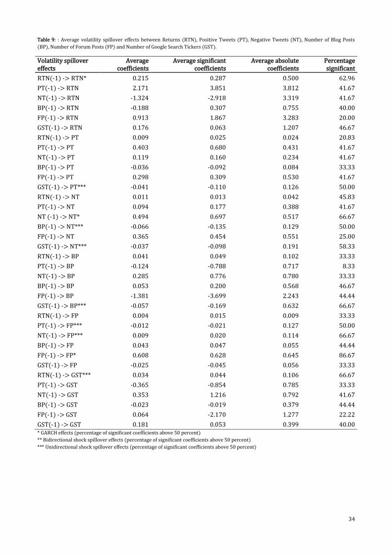
34

Table 9: : Average volatility spillover effects between Returns (RTN), Positive Tweets (PT), Negative Tweets (NT), Number of Blog Posts

(BP), Number of Forum Posts (FP) and Number of Google Search Tickers (GST).

* GARCH effects (percentage of significant coefficients above 50 percent)

** Bidirectional shock spillover effects (percentage of significant coefficients above 50 percent)

*** Unidirectional shock spillover effects (percentage of significant coefficients above 50 percent)

Volatility spillover effects

Average coefficients

Average significant coefficients

Average absolute coefficients

Percentage significant

RTN(-1) -> RTN* 0.215 0.287 0.500 62.96

PT(-1) -> RTN 2.171 3.851 3.812 41.67

NT(-1) -> RTN -1.324 -2.918 3.319 41.67

BP(-1) -> RTN -0.188 0.307 0.755 40.00

FP(-1) -> RTN 0.913 1.867 3.283 20.00

GST(-1) -> RTN 0.176 0.063 1.207 46.67

RTN(-1) -> PT 0.009 0.025 0.024 20.83

PT(-1) -> PT 0.403 0.680 0.431 41.67

NT(-1) -> PT 0.119 0.160 0.234 41.67

BP(-1) -> PT -0.036 -0.092 0.084 33.33

FP(-1) -> PT 0.298 0.309 0.530 41.67

GST(-1) -> PT*** -0.041 -0.110 0.126 50.00

RTN(-1) -> NT 0.011 0.013 0.042 45.83

PT(-1) -> NT 0.094 0.177 0.388 41.67

NT (-1) -> NT* 0.494 0.697 0.517 66.67

BP(-1) -> NT*** -0.066 -0.135 0.129 50.00

FP(-1) -> NT 0.365 0.454 0.551 25.00

GST(-1) -> NT*** -0.037 -0.098 0.191 58.33

RTN(-1) -> BP 0.041 0.049 0.102 33.33

PT(-1) -> BP -0.124 -0.788 0.717 8.33

NT(-1) -> BP 0.285 0.776 0.780 33.33

BP(-1) -> BP 0.053 0.200 0.568 46.67

FP(-1) -> BP -1.381 -3.699 2.243 44.44

GST(-1) -> BP*** -0.057 -0.169 0.632 66.67

RTN(-1) -> FP 0.004 0.015 0.009 33.33

PT(-1) -> FP*** -0.012 -0.021 0.127 50.00

NT(-1) -> FP*** 0.009 0.020 0.114 66.67

BP(-1) -> FP 0.043 0.047 0.055 44.44

FP(-1) -> FP* 0.608 0.628 0.645 86.67

GST(-1) -> FP -0.025 -0.045 0.056 33.33

RTN(-1) -> GST*** 0.034 0.044 0.106 66.67

PT(-1) -> GST -0.365 -0.854 0.785 33.33

NT(-1) -> GST 0.353 1.216 0.792 41.67

BP(-1) -> GST -0.023 -0.019 0.379 44.44

FP(-1) -> GST 0.064 -2.170 1.277 22.22

GST(-1) -> GST 0.181 0.053 0.399 40.00

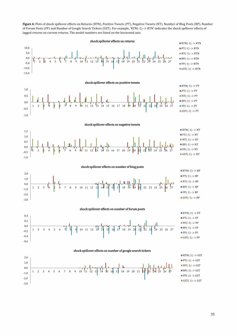
35

Figure 4: Plots of shock spillover effects on Returns (RTN), Positive Tweets (PT), Negative Tweets (NT), Number of Blog Posts (BP), Number

of Forum Posts (FP) and Number of Google Search Tickers (GST). For example, ‘RTN(-1) -> RTN’ indicates the shock spillover effects of

lagged returns on current returns. The model numbers are listed on the horizontal axis.

-15,0

-10,0

-5,0

0,0

5,0

10,0

1 2 3 4 5 6 7 8 9 10 11 12 13 14 15 16 17 18 19 20 21 22 23 24 25 26 27

shock spillover effects on returns RTN(-1) -> RTN

PT(-1) -> RTN

NT(-1) -> RTN

BP(-1) -> RTN

FP(-1) -> RTN

GST(-1) -> RTN

-1,0

-0,5

0,0

0,5

1,0

1 2 3 4 5 6 7 8 9 10 11 12 13 14 15 16 17 18 19 20 21 22 23 24 25 26 27

shock spillover effects on positive tweets RTN(-1) -> PT

PT(-1) -> PT

NT(-1) -> PT

BP(-1) -> PT

FP(-1) -> PT

GST(-1) -> PT

-1,0

-0,5

0,0

0,5

1,0

1,5

1 2 3 4 5 6 7 8 9 10 11 12 13 14 15 16 17 18 19 20 21 22 23 24 25 26 27

shock spillover effects on negative tweets

RTN(-1) -> NT

PT(-1) -> NT

NT(-1) -> NT

BP(-1) -> NT

FP(-1) -> NT

GST(-1) -> NT

-3,0

-2,0

-1,0

0,0

1,0

2,0

1 2 3 4 5 6 7 8 9 10 11 12 13 14 15 16 17 18 19 20 21 22 23 24 25 26 27

shock spillover effects on number of blog posts RTN(-1) -> BP

PT(-1) -> BP

NT(-1) -> BP

BP(-1) -> BP

FP(-1) -> BP

GST(-1) -> BP

-0,6

-0,4

-0,2

0,0

0,2

0,4

1 2 3 4 5 6 7 8 9 10 11 12 13 14 15 16 17 18 19 20 21 22 23 24 25 26 27

shock spillover effects on number of forum posts RTN(-1) -> FP

PT(-1) -> FP

NT(-1) -> FP

BP(-1) -> FP

FP(-1) -> FP

GST(-1) -> FP

-3,0

-2,0

-1,0

0,0

1,0

2,0

1 2 3 4 5 6 7 8 9 10 11 12 13 14 15 16 17 18 19 20 21 22 23 24 25 26 27

shock spillover effects on number of google search tickers

RTN(-1) -> GST

PT(-1) -> GST

NT(-1) -> GST

BP(-1) -> GST

FP(-1) -> GST

GST(-1) -> GST

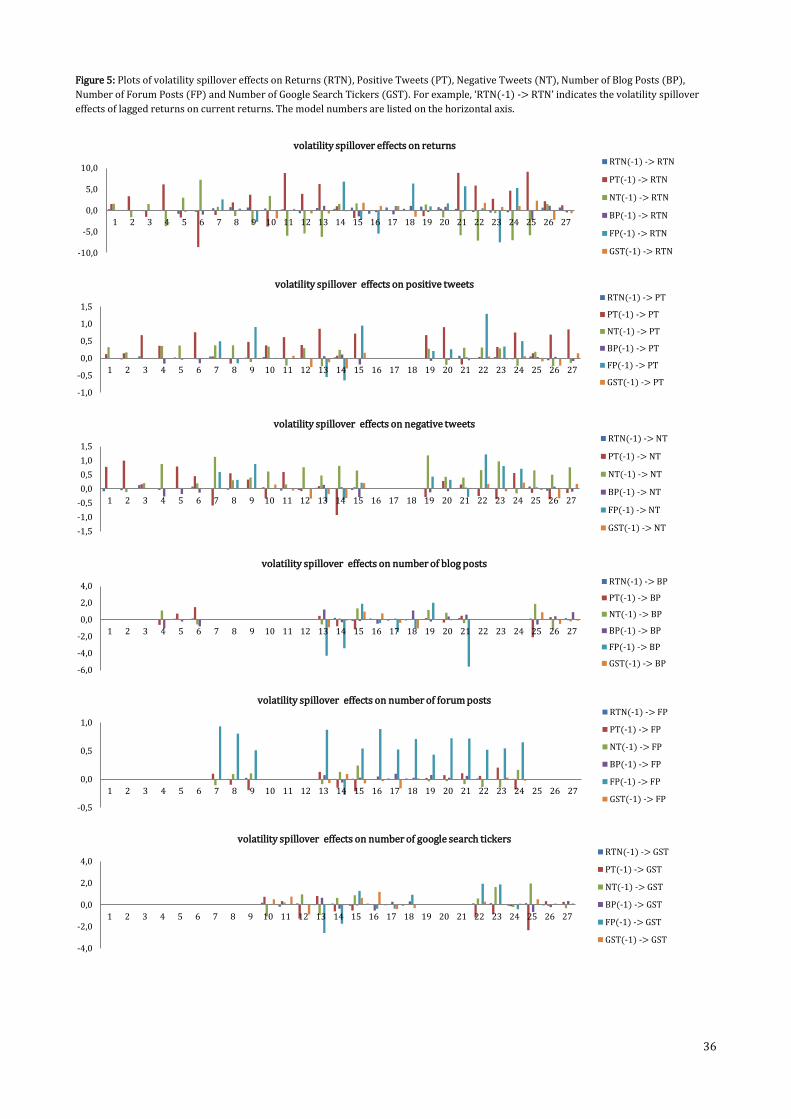
36

Figure 5: Plots of volatility spillover effects on Returns (RTN), Positive Tweets (PT), Negative Tweets (NT), Number of Blog Posts (BP),

Number of Forum Posts (FP) and Number of Google Search Tickers (GST). For example, ‘RTN(-1) -> RTN’ indicates the volatility spillover

effects of lagged returns on current returns. The model numbers are listed on the horizontal axis.

-10,0

-5,0

0,0

5,0

10,0

1 2 3 4 5 6 7 8 9 10 11 12 13 14 15 16 17 18 19 20 21 22 23 24 25 26 27

volatility spillover effects on returns

RTN(-1) -> RTN

PT(-1) -> RTN

NT(-1) -> RTN

BP(-1) -> RTN

FP(-1) -> RTN

GST(-1) -> RTN

-1,0

-0,5

0,0

0,5

1,0

1,5

1 2 3 4 5 6 7 8 9 10 11 12 13 14 15 16 17 18 19 20 21 22 23 24 25 26 27

volatility spillover effects on positive tweets RTN(-1) -> PT

PT(-1) -> PT

NT(-1) -> PT

BP(-1) -> PT

FP(-1) -> PT

GST(-1) -> PT

-1,5

-1,0

-0,5

0,0

0,5

1,0

1,5

1 2 3 4 5 6 7 8 9 10 11 12 13 14 15 16 17 18 19 20 21 22 23 24 25 26 27

volatility spillover effects on negative tweets

RTN(-1) -> NT

PT(-1) -> NT

NT(-1) -> NT

BP(-1) -> NT

FP(-1) -> NT

GST(-1) -> NT

-6,0

-4,0

-2,0

0,0

2,0

4,0

1 2 3 4 5 6 7 8 9 10 11 12 13 14 15 16 17 18 19 20 21 22 23 24 25 26 27

volatility spillover effects on number of blog posts

RTN(-1) -> BP

PT(-1) -> BP

NT(-1) -> BP

BP(-1) -> BP

FP(-1) -> BP

GST(-1) -> BP

-0,5

0,0

0,5

1,0

1 2 3 4 5 6 7 8 9 10 11 12 13 14 15 16 17 18 19 20 21 22 23 24 25 26 27

volatility spillover effects on number of forum posts RTN(-1) -> FP

PT(-1) -> FP

NT(-1) -> FP

BP(-1) -> FP

FP(-1) -> FP

GST(-1) -> FP

-4,0

-2,0

0,0

2,0

4,0

1 2 3 4 5 6 7 8 9 10 11 12 13 14 15 16 17 18 19 20 21 22 23 24 25 26 27

volatility spillover effects on number of google search tickers RTN(-1) -> GST

PT(-1) -> GST

NT(-1) -> GST

BP(-1) -> GST

FP(-1) -> GST

GST(-1) -> GST

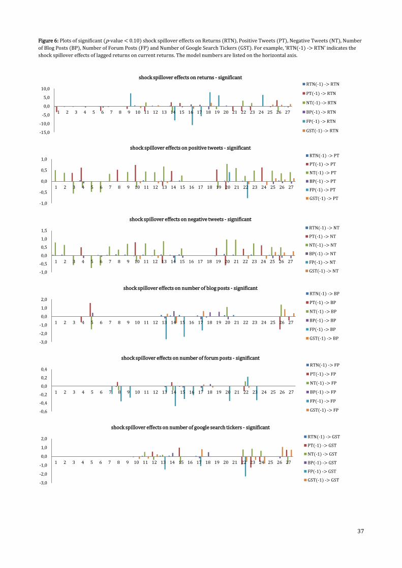
37

Figure 6: Plots of significant (p-value < 0.10) shock spillover effects on Returns (RTN), Positive Tweets (PT), Negative Tweets (NT), Number

of Blog Posts (BP), Number of Forum Posts (FP) and Number of Google Search Tickers (GST). For example, ‘RTN(-1) -> RTN’ indicates the

shock spillover effects of lagged returns on current returns. The model numbers are listed on the horizontal axis.

-15,0

-10,0

-5,0

0,0

5,0

10,0

1 2 3 4 5 6 7 8 9 10 11 12 13 14 15 16 17 18 19 20 21 22 23 24 25 26 27

shock spillover effects on returns - significant RTN(-1) -> RTN

PT(-1) -> RTN

NT(-1) -> RTN

BP(-1) -> RTN

FP(-1) -> RTN

GST(-1) -> RTN

-1,0

-0,5

0,0

0,5

1,0

1 2 3 4 5 6 7 8 9 10 11 12 13 14 15 16 17 18 19 20 21 22 23 24 25 26 27

shock spillover effects on positive tweets - significant

RTN(-1) -> PT

PT(-1) -> PT

NT(-1) -> PT

BP(-1) -> PT

FP(-1) -> PT

GST(-1) -> PT

-1,0

-0,5

0,0

0,5

1,0

1,5

1 2 3 4 5 6 7 8 9 10 11 12 13 14 15 16 17 18 19 20 21 22 23 24 25 26 27

shock spillover effects on negative tweets - significant

RTN(-1) -> NT

PT(-1) -> NT

NT(-1) -> NT

BP(-1) -> NT

FP(-1) -> NT

GST(-1) -> NT

-3,0

-2,0

-1,0

0,0

1,0

2,0

1 2 3 4 5 6 7 8 9 10 11 12 13 14 15 16 17 18 19 20 21 22 23 24 25 26 27

shock spillover effects on number of blog posts - significant RTN(-1) -> BP

PT(-1) -> BP

NT(-1) -> BP

BP(-1) -> BP

FP(-1) -> BP

GST(-1) -> BP

-0,6

-0,4

-0,2

0,0

0,2

0,4

1 2 3 4 5 6 7 8 9 10 11 12 13 14 15 16 17 18 19 20 21 22 23 24 25 26 27

shock spillover effects on number of forum posts - significant

RTN(-1) -> FP

PT(-1) -> FP

NT(-1) -> FP

BP(-1) -> FP

FP(-1) -> FP

GST(-1) -> FP

-3,0

-2,0

-1,0

0,0

1,0

2,0

1 2 3 4 5 6 7 8 9 10 11 12 13 14 15 16 17 18 19 20 21 22 23 24 25 26 27

shock spillover effects on number of google search tickers - significant

RTN(-1) -> GST

PT(-1) -> GST

NT(-1) -> GST

BP(-1) -> GST

FP(-1) -> GST

GST(-1) -> GST

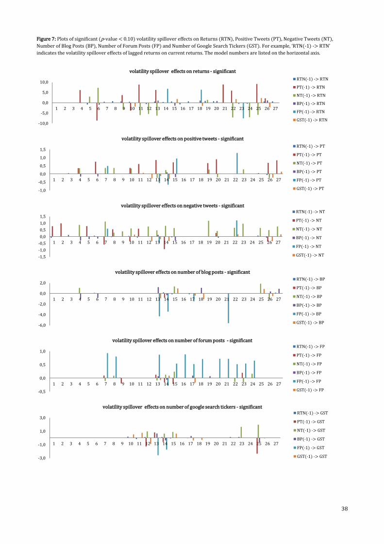
38

Figure 7: Plots of significant (p-value < 0.10) volatility spillover effects on Returns (RTN), Positive Tweets (PT), Negative Tweets (NT),

Number of Blog Posts (BP), Number of Forum Posts (FP) and Number of Google Search Tickers (GST). For example, ‘RTN(-1) -> RTN’

indicates the volatility spillover effects of lagged returns on current returns. The model numbers are listed on the horizontal axis.

-10,0

-5,0

0,0

5,0

10,0

1 2 3 4 5 6 7 8 9 10 11 12 13 14 15 16 17 18 19 20 21 22 23 24 25 26 27

volatility spillover effects on returns - significant

RTN(-1) -> RTN

PT(-1) -> RTN

NT(-1) -> RTN

BP(-1) -> RTN

FP(-1) -> RTN

GST(-1) -> RTN

-1,0

-0,5

0,0

0,5

1,0

1,5

1 2 3 4 5 6 7 8 9 10 11 12 13 14 15 16 17 18 19 20 21 22 23 24 25 26 27

volatility spillover effects on positive tweets - significant

RTN(-1) -> PT

PT(-1) -> PT

NT(-1) -> PT

BP(-1) -> PT

FP(-1) -> PT

GST(-1) -> PT

-1,5

-1,0

-0,5

0,0

0,5

1,0

1,5

1 2 3 4 5 6 7 8 9 10 11 12 13 14 15 16 17 18 19 20 21 22 23 24 25 26 27

volatility spillover effects on negative tweets - significant RTN(-1) -> NT

PT(-1) -> NT

NT(-1) -> NT

BP(-1) -> NT

FP(-1) -> NT

GST(-1) -> NT

-6,0

-4,0

-2,0

0,0

2,0

1 2 3 4 5 6 7 8 9 10 11 12 13 14 15 16 17 18 19 20 21 22 23 24 25 26 27

volatility spillover effects on number of blog posts - significant

RTN(-1) -> BP

PT(-1) -> BP

NT(-1) -> BP

BP(-1) -> BP

FP(-1) -> BP

GST(-1) -> BP

-0,5

0,0

0,5

1,0

1 2 3 4 5 6 7 8 9 10 11 12 13 14 15 16 17 18 19 20 21 22 23 24 25 26 27

volatility spillover effects on number of forum posts - significant RTN(-1) -> FP

PT(-1) -> FP

NT(-1) -> FP

BP(-1) -> FP

FP(-1) -> FP

GST(-1) -> FP

-3,0

-1,0

1,0

3,0

1 2 3 4 5 6 7 8 9 10 11 12 13 14 15 16 17 18 19 20 21 22 23 24 25 26 27

volatility spillover effects on number of google search tickers - significant RTN(-1) -> GST

PT(-1) -> GST

NT(-1) -> GST

BP(-1) -> GST

FP(-1) -> GST

GST(-1) -> GST

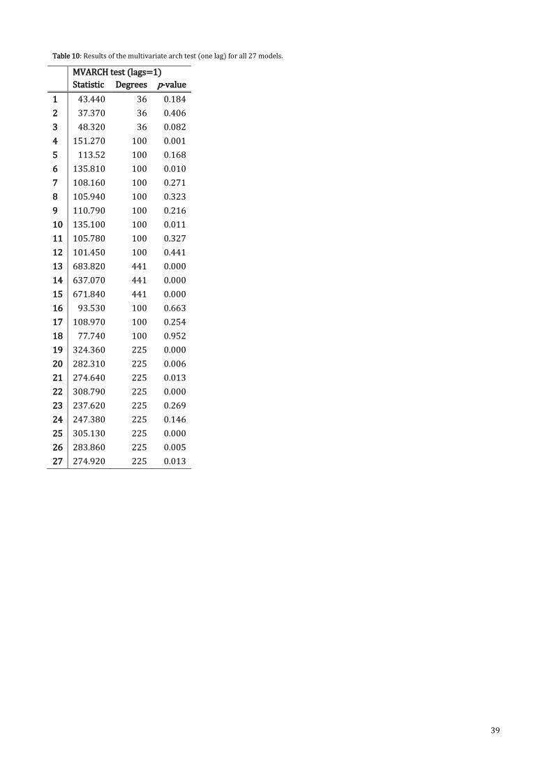
39

Table 10: Results of the multivariate arch test (one lag) for all 27 models.

MVARCH test (lags=1)

Statistic Degrees p-value

1 43.440 36 0.184

2 37.370 36 0.406

3 48.320 36 0.082

4 151.270 100 0.001

5 113.52 100 0.168

6 135.810 100 0.010

7 108.160 100 0.271

8 105.940 100 0.323

9 110.790 100 0.216

10 135.100 100 0.011

11 105.780 100 0.327

12 101.450 100 0.441

13 683.820 441 0.000

14 637.070 441 0.000

15 671.840 441 0.000

16 93.530 100 0.663

17 108.970 100 0.254

18 77.740 100 0.952

19 324.360 225 0.000

20 282.310 225 0.006

21 274.640 225 0.013

22 308.790 225 0.000

23 237.620 225 0.269

24 247.380 225 0.146

25 305.130 225 0.000

26 283.860 225 0.005

27 274.920 225 0.013

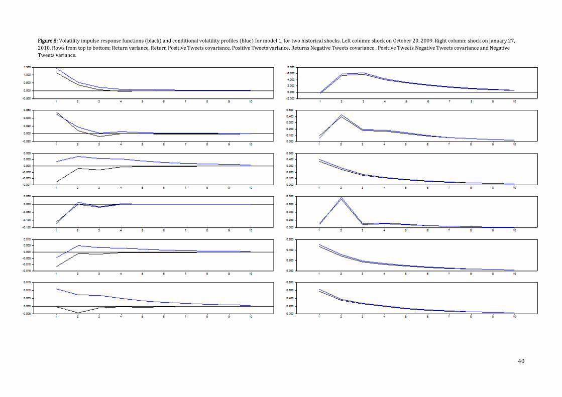
40

Figure 8: Volatility impulse response functions (black) and conditional volatility profiles (blue) for model 1, for two historical shocks. Left column: shock on October 20, 2009. Right column: shock on January 27,

2010. Rows from top to bottom: Return variance, Return Positive Tweets covariance, Positive Tweets variance, Returns Negative Tweets covariance , Positive Tweets Negative Tweets covariance and Negative

Tweets variance.

41

6. Discussion

This is the first study to investigate the presence of shock and volatility spillover effects between user

generated content and stock returns. With volatility being an important proxy of risk in the stock

market, influences on the volatility of stocks can present important insights in the fields of asset

pricing, portfolio optimization, risk management and option pricing. The direct relationship between

UGC and stock market performance has been investigated by Tirunillai and Tellis(2012) and Luo

(2007, 2009). Those studies were the first to examine the dynamics between UGC and stock market

performance; previous studies had merely focussed on examining the dynamics between UGC and

sales. Our study adds to the existing literature by not only investigating the direct connection between

UGC metrics and returns, but by investigating the connection between the volatilities of UGC metrics

and returns as well. Hence, our findings of spillovers between UGC and returns contribute to

unravelling the dynamics between UGC and stock market performance. According to these findings

there are more significant shock and volatility spillover effects from UGC sources to returns than vice

versa. The impact on the volatility of returns depends on the type of UGC source, some exhibit more

spillover effects than others. With these findings in mind, investors could be able to anticipate possible

changes in the volatility of a company’s stock by reviewing the volatility in UGC regarding that

company.

The multivariate GARCH BEKK model we used for our analysis is certainly the most suitable for

investigating shock and volatility spillover effects within our data, opposed to other multivariate

GARCH models such as the VECH model (too many parameters and the need to impose constraints to

ensure positive definiteness), the Diagonal BEKK and VECH model (can only measure ARCH and

GARCH effects, spillovers are not estimated in those models), the Constant Correlation model

(assumes that the covariances are generated with a constant, but unknown, correlation and therefore

might be too restrictive for our analysis), the Dynamic Correlation model (unrealistic assumption that

all entries in the conditional correlation matrix are influenced by the same coefficients) and the factor

model (the common factors size (SMB), market-to-book (HML) or momentum are not applicable to

our dataset).14

One aspect of the BEKK model we should be alert to is the fact that the model assumes that positive

and negative shocks have an equal impact. If that is not considered to be a realistic assumption, the

asymmetric BEKK model can be used, which takes into account whether shocks are positive or

negative. The asymmetric BEKK model has a larger number of parameters than the ‘regular’ BEKK

model we use in our study. Considering the small dataset we use we decided not to increase the

number of parameters to be estimated by employing an asymmetric version of the BEKK model. If in

14 We recognize that using ‘model-free’ realized volatility measures to study spillover effects would have been a possibility as well, but the advantages of the multivariate GARCH BEKK model to study spillover effects were crucial for our decision to use a multivariate GARCH model. Other options could be explored in further research.

42

time more data can be collected this would be worthwhile to explore. The same applies to

incorporating seasonality effects: with a larger sample it should not be a problem to add extra

dummies to the BEKK model. With our current relatively small sample this is not preferable. The curse

of dimensionality associated with estimating a BEKK model with a small sample might lead to

problems as overfitting or numerical instabilities (Verleysen and François, 2005). Correcting for this

curse of dimensionality can be quite cumbersome and would be a new study in itself, which is why for

our study we choose to estimate 27 models with both small and larger combinations of variables, of

which we presented the summarized results (the ‘meta-analysis’). A risk we take with our analysis is

the possibility that some of the smaller models may be misspecified, as other (important) variables are

omitted.

A drawback of our meta-analysis is that the averages of the effects are calculated of different totals.

For instance, the shock and volatility spillover effects between returns and the volume of positive

tweets are estimated in 24 models and the average of those spillovers are computed over the 24

estimates. The shock and volatility spillover effects between the number of blog posts and the number

of Google search tickers are estimated in only 9 models and the averages are therefore computed over

just 9 estimates. When the average is calculated over fewer models, one estimate can have relatively

more influence. Not only can one value have a bigger impact on the value of the coefficient, the

percentage of significant coefficients is affected as well. In the previous chapter we mainly focussed on

the results that are significant in at least 50 percent of the estimates, but 50 percent over 9 estimates is

of course different than 50 percent over 24 estimates. When an effect is estimated in 15, 24 or 27

models and the percentage of significant coefficients is high, we can state that with greater certainty

that this particular effect is significant (on average) than when it would have been estimated over just

9 models. Hence, average effects that are significant in at least 75 percent of the estimates and are

estimated in at least 15 models allow us to draw conclusions with bigger empirical certainty. There are

four effects present in our results that match these criteria: the shock spillover effect from negative

tweets to positive tweets; the shock spillover effect from returns to negative tweets, the ARCH effect in

the volume negative tweets and the GARCH effect in the number of forum posts. The strong connection

between negative tweets and positive tweets makes sense, as Twitter uses hashtags for topics, to

which tweets are linked (after each tweet follows ‘#topic’). Shocks in the volume of negative tweets

are therefore likely to be linked to shocks in positive tweets, as people tend to have various opinions

about a topic. The shock spillovers from returns to negative tweets might be explained by the fact that

shocks in stock returns are associated with higher risk, and therefore might trigger negative responses

rather than positive responses on Twitter. The effect is small, which is probably due to the fact that the

negative tweets in our dataset are about the product iPhone of Apple, not about the company Apple in

general.

43

With time, the analysis could be extended in various ways. One approach would be to collect similar

data and perform a similar analysis for companies other than Apple. This paper is a case-study of

Apple and performing our analysis on other companies could serve to verify whether the linkages

between stock returns and UGC extend to other companies as well. Furthermore, if the analysis could

be performed for companies in different industries, we could investigate whether the stocks of

companies in certain industries are more prone to shock and volatility spillovers from online content

than stocks of companies in different industries. Another approach would be to collect new UGC data

regarding Apple, but not just content about the iPhone, but about all products of Apple, among which

the computers and iPad. The iPad had been launched, but was not available to the public in the period

of our dataset. We assume that there will be much UGC about this product as well after it was made

available to the public, as it has now grown out to be one of the most iconic product of Apple. Since the

wide range of products of Apple all contribute to the performance of the company and all influence the

way consumers view the company, we might find stronger linkages between stock returns and UGC

when more of Apple’s product are taken into account in the dataset. All of the aforementioned

approaches would allow us to get greater empirical certainty on the nature and significance of the

mean, shock and volatility spillovers between stock returns and UGC.

44

7. Conclusion

This study examines the dynamics between user-generated content (UGC) and stock returns by

investigating the presence of mean, shock and volatility spillover effects between UGC and returns

related to the company Apple. The volume of positive and negative tweets, the number of blog posts

and forum posts and the number of searches for the Apple ticker symbol in the Google search engine

are used as metrics of UGC. We collected the UGC data over a six month period (from October 2009

until March 2010), using various online sources. The multivariate GARCH BEKK model is used to study

the source, significance and magnitude of the mean, shock and volatility spillover. We perform a meta-

analysis to study the spillover effects between UGC variables and Returns by estimating 27

multivariate GARCH BEKK models using various combinations of variables and computed averages

over the results of those 27 models. These results confirm the presence of the mean, shock and

volatility spillover effects and show that the spillovers from UGC to returns are bigger (and are

significant in more of the estimates) than from returns to UGC. There are spillovers between the

various UGC sources as well and these effects are bigger (and are significant in more of the estimates)

than the effect of returns on UGC. Hence, online content is influenced more by other online content

than by stock returns. Furthermore, the results show that both the magnitude and sign of the shock

and volatility spillover effects between stock returns and UGC and among UGC sources differ per UGC

measure. The effects of positive tweets versus the effects of negative tweets show us that the spillovers

differ in magnitude, significance and sign depending on whether online content is positive or negative.

Negative tweets have a slightly bigger impact (and are significant in more of the estimates) than

positive tweets in most cases, which might be due to the fact that people are more inclined to focus on

negative than on positive news (negativity bias). New product launches and organizational events

partly explain the variance and covariance between UGC and stock returns and the Volatility Impulse

Response Functions and conditional volatility profiles show that new product launches can cause a

shock in (co)variances of stock returns and UGC. The impact of the shock depends on the product

being launched, judging from the different responses in our results.

Considering that this is the first study to examine the dynamics between UGC and stock returns in

terms of mean, shock and volatility spillovers, we recommend to perform a similar study to a different

company, preferably in a different industry, in order to obtain greater empirical certainty about these

spillover effects.

45

8. References

Alom, F., Ward, B.D. and Hu, B. (2011) Cross country mean and volatility spillover effects of food

prices: multivariate GARCH analysis. Economics Bulletin, 31(2):1439-1450.

Andersen, T.G., Bollerslev, T., Diebold, F.X. and Vega, C. (2003) Micro effects of macro announcements:

real-time price discovery in foreign exchange. The American Economic Review, 93(1):38-62.

Andersen, T.G., Bollerslev, T., Diebold, F.X. and Vega, C. (2007) Real-time price discovery in global

stock, bond and foreign exchange markets. Journal of International Economics, 73:251-277.

Asur, S., Huberman, B.A. (2010) Predicting the Future with Social Media. Working paper:

arXiv:1003.5699v1

Bauwens, L., Laurent, S. and Rombouts, J.V.K. (2006) Multivariate GARCH Models: A Survey. Journal of

Applied Econometrics, 21:79-109.

Berger, J. and Milkman, K.L. (2012) What makes online content viral? Journal of Marketing Research,

49(1):192-206.

Bollen, J., Mao, H., Zeng, X.J. (2011) Twitter mood predicts the stock market. Journal of Computational

Science, 2:1-8.

Bollerslev, T., Chou, R. and Kroner, K. (1992) ARCH modelling in finance: A review of the theory and

empirical evidence. Journal of Econometrics, 52:5-59.

Bollerslev, T., Engle, R. and Woolridge, J. (1988) A Capital Asset Pricing Model with Time-varying

Covariances. Journal of Political Economy, 96:116-131.

Brooks, C., Burke, S. and Persand, G. (2003) Multivariate GARCH Models: Software Choice and

Estimation Issues. ISMA Centre Discussion Papers in Finance DP2003-07.

Brooks, C., Li, X. and Miffre, J. (2009) Time-Varying Volatility and the Cross-Section of Equity Returns.

ICMA Centre Discussion Papers in Finance DP2009-01.

Caldeira, J., Moura, G. and Santos, A.A.P. (2012) Portfolio optimization using a parsimonious

multivariate GARCH model: application to the Brazilian stock market. Economics Bulletin, 32(3):1848-

1857.

Carhart, M.M. (1997) On Persistence in Mutual Fund Performance. Journal of Finance, 52(1):57-82.

Chevalier, J.A. and Mayzlin, D. (2006) The Effect of Word-of-Mouth on Sales: Online Book Reviews.

Journal of Marketing Research, 43:345-354.

46

Choi, H. and Varian, H. (2011) Predicting the Present with Google Trends. Google Inc. Technical Report.

Choudhry, T. and Wu, H. (2008) Forecasting Ability of GARCH vs Kalman Filter Method: Evidence from

Daily UK Time-Varying Beta. Journal of Forecasting, 27:670-689.

Christoffersen, P. and Jacobs, K. (2004) Which GARCH Model for Option Valuation? Management

Science, 50(9):1204-1221.

Conn, R.R. (2011) A Primer on the Nature of Idiosyncratic Risk and Volatility. The value examiner

September/October 2011, 13-19.

Dhar, V., Chang, E.A. (2009) Does Chatter Matter? The Impact of User-Generated Content on Music

Sales. Journal of Interactive Marketing, 23:300-307.

Doan, T.A. (2013) RATS Handbook for ARCH/GARCH and Volatility Models. Estima WINRATS.

eMarketer (2010) http://www.bazaarvoice.com/research-and-insight/social-commerce-statistics

Elyasiani, E., Perera, P. and Puri, T.N. (1998) Interdependence and dynamic linkages between stock

markets of Sri Lanka and its trading partners. Journal of Multinational Financial Management, 8:89-

101.

Engle, R.F. (2001) GARCH 101: The Use of ARCH/GARCH Models in Applied Econometrics. Journal of

Economic Perspectives, 15(4):157-168.

Engle, R.F., Ito, T. and Lin, W. (1990) Meteor Showers or Heat Waves? Heteroskedastic Intra- Daily

Volatility in the Foreign Exchange Market, Econometrica, 58:525-542.

Engle, R.F. and Ng, V.K. (1993) Measuring and Testing the Impact of News on Volatility. The Journal of

Finance, 48(5):1749:1778.

Engle, R.F. and Kroner, K.F. (1995) Multivariate simultaneous generalized ARCH. Economic Theory,

11:122-150.

Fama, E.F. and French, K.R. (1993) Common risk factors in the returns on stocks and bonds. Journal of

Financial Economics, 33: 3-56.

Fama, E.F. and French, K.R. (2004) The Capital Asset Pricing Model: Theory and Evidence. Journal of

Economic Perspectives, 18(3):25-46.

Franses, P.H. and Van Dijk, D. (2000) Nonlinear Time Series Models in Empirical Finance. Cambridge

University Press

47

Gilbert, E., Karahalios, K. (2010) Widespread worry and the stock market. Proceedings of the 4th

International AAAI (Association for the Advancement of Artificial Intelligence) Conference on Weblogs

and Social Media, ICWSM.

Glabadanidis, P. (2009) A Dynamic Asset Pricing Model with Time-Varying Factor and Idiosyncratic

Risk. Journal of Financial Econometrics, 7(3):247-264.

Godes, D. and Mayzlin, D. (2004) Using Online Conversations to Study Word-of-Mouth Communication.

Marketing Science, 23(4):545-560.

Goldenberg, J., Oestreicher-Singer, G. and Reichman, S. (2012) The Quest for Content: How User-

Generated Links Can Facilitate Online Exploration. Journal of Marketing Research, 49:452-468.

Gruhl, D., Guha, R., Kumar, R., Novak, J., Tomkins, A. (2005) The predictive power of online chatter.

ACM, New York, NY, USA, 78-87.

Joshi, P. (2011) Return and Volatility Spillovers among Asian stock markets. SAGE Open, 1:1-8.

Joshi, A., Hanssens, D.M. (2010) The Direct and Indirect Effects of Advertising Spending on Firm Value.

Journal of Marketing, 74:20-33.

Kelton Research (2011) http://www.bazaarvoice.com/research-and-insight/social-commerce-

statistics

Li, X., Hitt, L. (2008) Self-Selection and Information Role of Online Product Reviews. Information

Systems Research, 19:456-474.

Li, H. and Majerowska, E. (2008) Testing stock market linkages for Poland and Hungary: A multivariate

GARCH approach. Research in International Business and Finance, 22(3):247-266.

Lin, S.L., Penm, J., Wu, S., Chiu, W.J. (2004) A Factor-GARCH approach to conditional risk and return in

banking stocks: comparison of industry effect in Taiwan, Hong Kong, and Mainland China. Working

paper, SSRN eLibrary.

Lintner, J. (1965) The valuation of risk assets and the selection of risky investments in stock portfolios

and capital budgets. Review of Economics and Statistics, 47:13-37.

Liu, Y., Huang, X., An, A., Yu, X. (2007) ARSA: a sentiment-aware model for predicting sales

performance using blogs. ACM, New York, NY, USA, 607-614.

Mishne, G., Glance, N. (2006) Predicting Movie Sales from Blogger Sentiment. AAAI (Association for the

Advancement of Artificial Intelligence) 2006 Spring Symposium on Computational Approaches to

Analysing Weblogs.

48

Najand, M., Lin, C.Y. and Fitzgerald, E. (2006) The Conditional CAPM and Time Varying Risk Premium

for Equity REITs. Journal of Real Estate Portfolio Management, 12(2):167-175.

Nath, H.B. (2012) An empirical investigation of idiosyncratic risk and stock returns relation in

heteroscedasticity corrected predictive models. In:

http://www.efmaefm.org/0EFMAMEETINGS/EFMA%20ANNUAL%20MEETINGS/2012-

Barcelona/papers/EFMA2012_0202_fullpaper.pdf

Nieto, B., Orbe, S. and Zarraga, A. (2010) Time-Varying Market Beta: Does the estimation methodology

matter? Working paper:

http://web.ua.es/es/researchgroupmffe/investigadores/documentos/nietodomenech/betas2.pdf

Pak, A., Paroubek, P. (2010) Twitter as a Corpus for Sentiment Analysis and Opinion Mining. In:

Calzolari, N., Choukri, K., Maegaard, B., Mar- iani, J., Odijk, J., Piperidis, S., Rosner, M., Tapias, D. (Eds.),

Proceedings of the Seventh conference on International Language Resources and Evaluation

(LREC’10). European Language Resources Association (ELRA), Valletta, Malta, May 19–21.

Piller, Charles (1999), “Everyone Is A Critic in Cyberspace,” Los Angeles Times, (December 3rd), A1.

Ransbotham, S., Kane, G.C., Lurie, N.H. (2012) Network Characteristics and the Value of Collaborative

User-Generated Content. Marketing Science, 31(3):387-405.

Setiawan, K. (2012) Reexamination of Dynamic Beta International CAPM: a SUR with GARCH

Approach. Review of Economic and Business Studies, 5(2):105-127.

Sharpe, W. (1964) Capital asset prices: a theory of market equilibrium under conditions of risk.

Journal of Finance, 19:425-442.

Starr, M.A. (2012) Consumption, sentiment and economic news. Economic Inquiry, 50(4):1097-1111.

Schumaker, R.P., Chen, H. (2009) Textual Analysis of Stock Market Prediction Using Breaking Financial

News: The AZFinText System. ACM Transactions on Information Systems, 27(2):Article 12.

Tellis, G.J. and Franses, P.H. (2006) Optimal data interval for estimating advertising response.

Marketing Science, 25(3):217-229.

Tellis, G.J. and Johnson, J. (2007) The value of quality. Marketing Science, 26(6):758-773.

Tirunillai, S. and Tellis, G.J. (2012) Does Chatter Really Matter? Dynamics of UGC and Stock

Performance. Marketing Science, 31(2):198-215.

Trusov, M., Bucklin, R. and Pauwels, K. (2009) Effects of word-of-mouth versus traditional marketing:

finding from an internet social networking site. Journal of Marketing, 73:90-102.

49

Verleysen, M. and François, D. (2005) The Curse of Dimensionality in Data Mining and Time Series

Prediction. Computational Intelligence and Bioinspired Systems, Lecture Notes in Computer Science,

3512:758-770.

Wang, C.W., Tzang, S.W., Wu, C.W. and Hung C.H. (2012) Systematic Risk in GARCH Option Pricing: A

Theoretical and Empirical Perspective. In:

http://www.researchgate.net/publication/228693018_Systematic_Risk_in_GARCH_Option_Pricing_A_

Theoretical_and_Empirical_Perspectives

Worthington, A. and Higgs, H. (2004). Transmission of Equity Returns And Volatility In Asian

Developed And Emerging Markets: A Multivariate Garch Analysis. International Journal of Finance and

Economics, 9(1):71

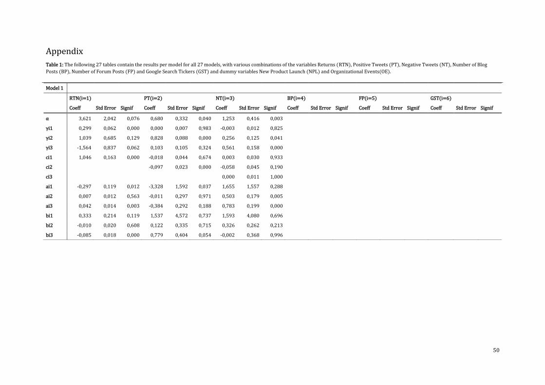
50

Appendix

Table 1: The following 27 tables contain the results per model for all 27 models, with various combinations of the variables Returns (RTN), Positive Tweets (PT), Negative Tweets (NT), Number of Blog

Posts (BP), Number of Forum Posts (FP) and Google Search Tickers (GST) and dummy variables New Product Launch (NPL) and Organizational Events(OE).

Model 1

RTN(i=1)

PT(i=2)

NT(i=3)

BP(i=4)

FP(i=5)

GST(i=6)

Coeff Std Error Signif Coeff Std Error Signif Coeff Std Error Signif Coeff Std Error Signif Coeff Std Error Signif Coeff Std Error Signif

α 3,621 2,042 0,076 0,680 0,332 0,040 1,253 0,416 0,003

γi1 0,299 0,062 0,000 0,000 0,007 0,983 -0,003 0,012 0,825

γi2 1,039 0,685 0,129 0,828 0,088 0,000 0,256 0,125 0,041

γi3 -1,564 0,837 0,062 0,103 0,105 0,324 0,561 0,158 0,000

ci1 1,046 0,163 0,000 -0,018 0,044 0,674 0,003 0,030 0,933

ci2 -0,097 0,023 0,000 -0,058 0,045 0,190

ci3 0,000 0,011 1,000

ai1 -0,297 0,119 0,012 -3,328 1,592 0,037 1,655 1,557 0,288

ai2 0,007 0,012 0,563 -0,011 0,297 0,971 0,503 0,179 0,005

ai3 0,042 0,014 0,003 -0,384 0,292 0,188 0,783 0,199 0,000

bi1 0,333 0,214 0,119 1,537 4,572 0,737 1,593 4,080 0,696

bi2 -0,010 0,020 0,608 0,122 0,335 0,715 0,326 0,262 0,213

bi3 -0,085 0,018 0,000 0,779 0,404 0,054 -0,002 0,368 0,996

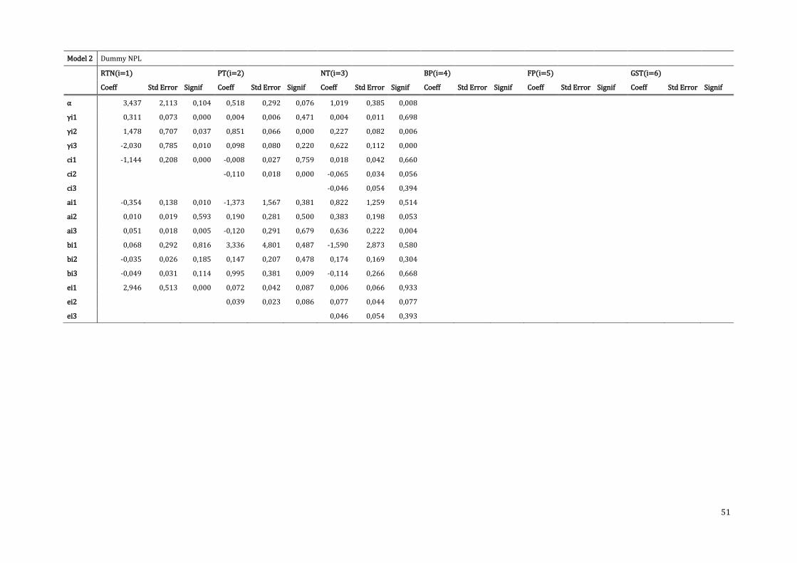
51

Model 2 Dummy NPL

RTN(i=1)

PT(i=2)

NT(i=3)

BP(i=4)

FP(i=5)

GST(i=6)

Coeff Std Error Signif Coeff Std Error Signif Coeff Std Error Signif Coeff Std Error Signif Coeff Std Error Signif Coeff Std Error Signif

α 3,437 2,113 0,104 0,518 0,292 0,076 1,019 0,385 0,008

γi1 0,311 0,073 0,000 0,004 0,006 0,471 0,004 0,011 0,698

γi2 1,478 0,707 0,037 0,851 0,066 0,000 0,227 0,082 0,006

γi3 -2,030 0,785 0,010 0,098 0,080 0,220 0,622 0,112 0,000

ci1 -1,144 0,208 0,000 -0,008 0,027 0,759 0,018 0,042 0,660

ci2

-0,110 0,018 0,000 -0,065 0,034 0,056

ci3

-0,046 0,054 0,394

ai1 -0,354 0,138 0,010 -1,373 1,567 0,381 0,822 1,259 0,514

ai2 0,010 0,019 0,593 0,190 0,281 0,500 0,383 0,198 0,053

ai3 0,051 0,018 0,005 -0,120 0,291 0,679 0,636 0,222 0,004

bi1 0,068 0,292 0,816 3,336 4,801 0,487 -1,590 2,873 0,580

bi2 -0,035 0,026 0,185 0,147 0,207 0,478 0,174 0,169 0,304

bi3 -0,049 0,031 0,114 0,995 0,381 0,009 -0,114 0,266 0,668

ei1 2,946 0,513 0,000 0,072 0,042 0,087 0,006 0,066 0,933

ei2

0,039 0,023 0,086 0,077 0,044 0,077

ei3

0,046 0,054 0,393

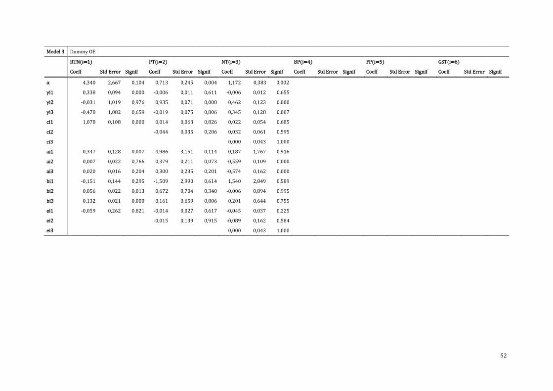
52

Model 3 Dummy OE

RTN(i=1)

PT(i=2)

NT(i=3)

BP(i=4)

FP(i=5)

GST(i=6)

Coeff Std Error Signif Coeff Std Error Signif Coeff Std Error Signif Coeff Std Error Signif Coeff Std Error Signif Coeff Std Error Signif

α 4,340 2,667 0,104 0,713 0,245 0,004 1,172 0,383 0,002

γi1 0,338 0,094 0,000 -0,006 0,011 0,611 -0,006 0,012 0,655

γi2 -0,031 1,019 0,976 0,935 0,071 0,000 0,462 0,123 0,000

γi3 -0,478 1,082 0,659 -0,019 0,075 0,806 0,345 0,128 0,007

ci1 1,078 0,108 0,000 0,014 0,063 0,826 0,022 0,054 0,685

ci2

-0,044 0,035 0,206 0,032 0,061 0,595

ci3

0,000 0,043 1,000

ai1 -0,347 0,128 0,007 -4,986 3,151 0,114 -0,187 1,767 0,916

ai2 0,007 0,022 0,766 0,379 0,211 0,073 -0,559 0,109 0,000

ai3 0,020 0,016 0,204 0,300 0,235 0,201 -0,574 0,162 0,000

bi1 -0,151 0,144 0,295 -1,509 2,990 0,614 1,540 2,849 0,589

bi2 0,056 0,022 0,013 0,672 0,704 0,340 -0,006 0,894 0,995

bi3 0,132 0,021 0,000 0,161 0,659 0,806 0,201 0,644 0,755

ei1 -0,059 0,262 0,821 -0,014 0,027 0,617 -0,045 0,037 0,225

ei2

-0,015 0,139 0,915 -0,089 0,162 0,584

ei3

0,000 0,043 1,000

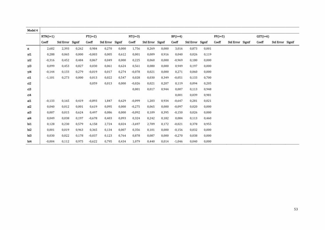
53

Model 4

RTN(i=1)

PT(i=2)

NT(i=3)

BP(i=4)

FP(i=5)

GST(i=6)

Coeff Std Error Signif Coeff Std Error Signif Coeff Std Error Signif Coeff Std Error Signif Coeff Std Error Signif Coeff Std Error Signif

α 2,682 2,393 0,262 0,984 0,270 0,000 1,756 0,269 0,000 3,016 0,873 0,001

γi1 0,288 0,065 0,000 -0,003 0,005 0,612 0,001 0,009 0,916 0,040 0,026 0,119

γi2 -0,316 0,452 0,484 0,867 0,049 0,000 0,225 0,060 0,000 -0,969 0,180 0,000

γi3 0,099 0,453 0,827 0,030 0,061 0,624 0,561 0,080 0,000 0,949 0,197 0,000

γi4 -0,144 0,133 0,279 -0,019 0,017 0,274 -0,078 0,021 0,000 0,271 0,060 0,000

ci1 -1,101 0,273 0,000 0,013 0,022 0,547 0,028 0,030 0,349 -0,051 0,133 0,700

ci2

0,059 0,013 0,000 -0,026 0,021 0,207 0,119 0,094 0,205

ci3

0,001 0,017 0,944 0,007 0,113 0,948

ci4

0,001 0,039 0,981

ai1 -0,133 0,165 0,419 -0,893 1,847 0,629 -0,099 1,203 0,934 -0,647 0,281 0,021

ai2 0,040 0,012 0,001 0,619 0,095 0,000 -0,275 0,065 0,000 -0,097 0,020 0,000

ai3 0,007 0,015 0,624 0,497 0,086 0,000 -0,092 0,109 0,395 -0,150 0,026 0,000

ai4 0,049 0,038 0,197 -0,678 0,403 0,093 0,324 0,242 0,182 0,084 0,113 0,460

bi1 0,128 0,230 0,579 6,158 2,724 0,024 -3,697 2,709 0,172 -0,021 0,378 0,955

bi2 0,001 0,019 0,963 0,365 0,134 0,007 0,356 0,101 0,000 -0,156 0,032 0,000

bi3 0,030 0,022 0,178 -0,037 0,123 0,764 0,878 0,087 0,000 -0,270 0,038 0,000

bi4 -0,004 0,112 0,975 -0,622 0,795 0,434 1,079 0,440 0,014 -1,046 0,040 0,000

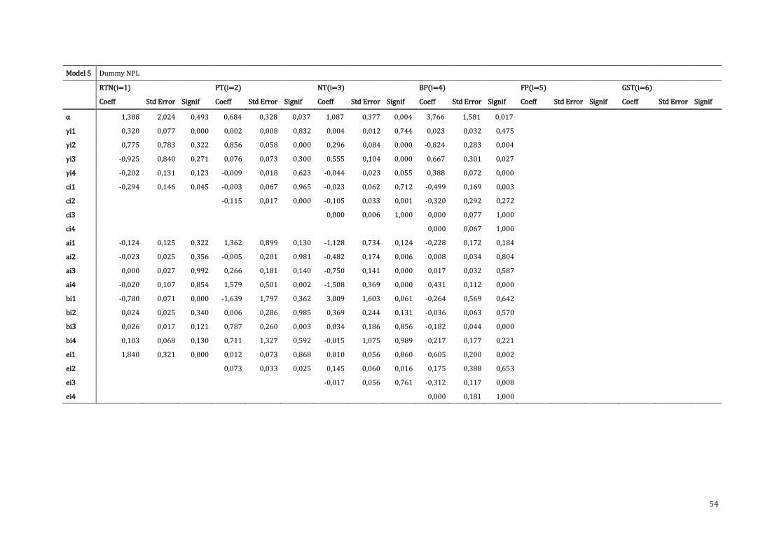
54

Model 5 Dummy NPL

RTN(i=1)

PT(i=2)

NT(i=3)

BP(i=4)

FP(i=5)

GST(i=6)

Coeff Std Error Signif Coeff Std Error Signif Coeff Std Error Signif Coeff Std Error Signif Coeff Std Error Signif Coeff Std Error Signif

α 1,388 2,024 0,493 0,684 0,328 0,037 1,087 0,377 0,004 3,766 1,581 0,017

γi1 0,320 0,077 0,000 0,002 0,008 0,832 0,004 0,012 0,744 0,023 0,032 0,475

γi2 0,775 0,783 0,322 0,856 0,058 0,000 0,296 0,084 0,000 -0,824 0,283 0,004

γi3 -0,925 0,840 0,271 0,076 0,073 0,300 0,555 0,104 0,000 0,667 0,301 0,027

γi4 -0,202 0,131 0,123 -0,009 0,018 0,623 -0,044 0,023 0,055 0,388 0,072 0,000

ci1 -0,294 0,146 0,045 -0,003 0,067 0,965 -0,023 0,062 0,712 -0,499 0,169 0,003

ci2

-0,115 0,017 0,000 -0,105 0,033 0,001 -0,320 0,292 0,272

ci3

0,000 0,006 1,000 0,000 0,077 1,000

ci4

0,000 0,067 1,000

ai1 -0,124 0,125 0,322 1,362 0,899 0,130 -1,128 0,734 0,124 -0,228 0,172 0,184

ai2 -0,023 0,025 0,356 -0,005 0,201 0,981 -0,482 0,174 0,006 0,008 0,034 0,804

ai3 0,000 0,027 0,992 0,266 0,181 0,140 -0,750 0,141 0,000 0,017 0,032 0,587

ai4 -0,020 0,107 0,854 1,579 0,501 0,002 -1,508 0,369 0,000 0,431 0,112 0,000

bi1 -0,780 0,071 0,000 -1,639 1,797 0,362 3,009 1,603 0,061 -0,264 0,569 0,642

bi2 0,024 0,025 0,340 0,006 0,286 0,985 0,369 0,244 0,131 -0,036 0,063 0,570

bi3 0,026 0,017 0,121 0,787 0,260 0,003 0,034 0,186 0,856 -0,182 0,044 0,000

bi4 0,103 0,068 0,130 0,711 1,327 0,592 -0,015 1,075 0,989 -0,217 0,177 0,221

ei1 1,840 0,321 0,000 0,012 0,073 0,868 0,010 0,056 0,860 0,605 0,200 0,002

ei2

0,073 0,033 0,025 0,145 0,060 0,016 0,175 0,388 0,653

ei3

-0,017 0,056 0,761 -0,312 0,117 0,008

ei4

0,000 0,181 1,000

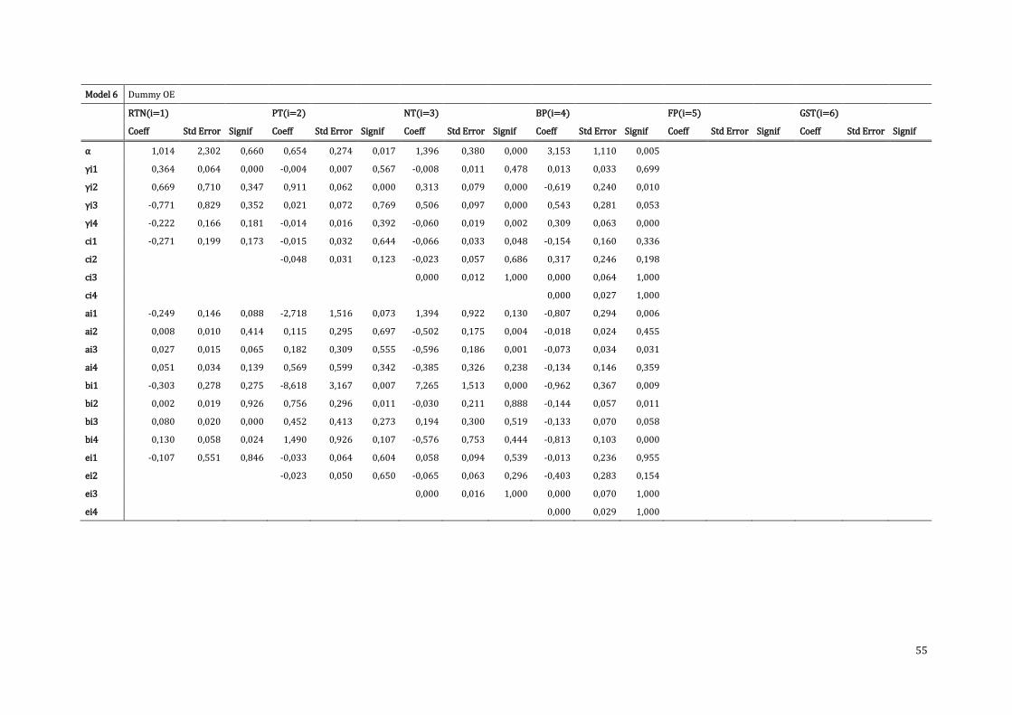
55

Model 6 Dummy OE

RTN(i=1)

PT(i=2)

NT(i=3)

BP(i=4)

FP(i=5)

GST(i=6)

Coeff Std Error Signif Coeff Std Error Signif Coeff Std Error Signif Coeff Std Error Signif Coeff Std Error Signif Coeff Std Error Signif

α 1,014 2,302 0,660 0,654 0,274 0,017 1,396 0,380 0,000 3,153 1,110 0,005

γi1 0,364 0,064 0,000 -0,004 0,007 0,567 -0,008 0,011 0,478 0,013 0,033 0,699

γi2 0,669 0,710 0,347 0,911 0,062 0,000 0,313 0,079 0,000 -0,619 0,240 0,010

γi3 -0,771 0,829 0,352 0,021 0,072 0,769 0,506 0,097 0,000 0,543 0,281 0,053

γi4 -0,222 0,166 0,181 -0,014 0,016 0,392 -0,060 0,019 0,002 0,309 0,063 0,000

ci1 -0,271 0,199 0,173 -0,015 0,032 0,644 -0,066 0,033 0,048 -0,154 0,160 0,336

ci2

-0,048 0,031 0,123 -0,023 0,057 0,686 0,317 0,246 0,198

ci3

0,000 0,012 1,000 0,000 0,064 1,000

ci4

0,000 0,027 1,000

ai1 -0,249 0,146 0,088 -2,718 1,516 0,073 1,394 0,922 0,130 -0,807 0,294 0,006

ai2 0,008 0,010 0,414 0,115 0,295 0,697 -0,502 0,175 0,004 -0,018 0,024 0,455

ai3 0,027 0,015 0,065 0,182 0,309 0,555 -0,596 0,186 0,001 -0,073 0,034 0,031

ai4 0,051 0,034 0,139 0,569 0,599 0,342 -0,385 0,326 0,238 -0,134 0,146 0,359

bi1 -0,303 0,278 0,275 -8,618 3,167 0,007 7,265 1,513 0,000 -0,962 0,367 0,009

bi2 0,002 0,019 0,926 0,756 0,296 0,011 -0,030 0,211 0,888 -0,144 0,057 0,011

bi3 0,080 0,020 0,000 0,452 0,413 0,273 0,194 0,300 0,519 -0,133 0,070 0,058

bi4 0,130 0,058 0,024 1,490 0,926 0,107 -0,576 0,753 0,444 -0,813 0,103 0,000

ei1 -0,107 0,551 0,846 -0,033 0,064 0,604 0,058 0,094 0,539 -0,013 0,236 0,955

ei2

-0,023 0,050 0,650 -0,065 0,063 0,296 -0,403 0,283 0,154

ei3

0,000 0,016 1,000 0,000 0,070 1,000

ei4

0,000 0,029 1,000

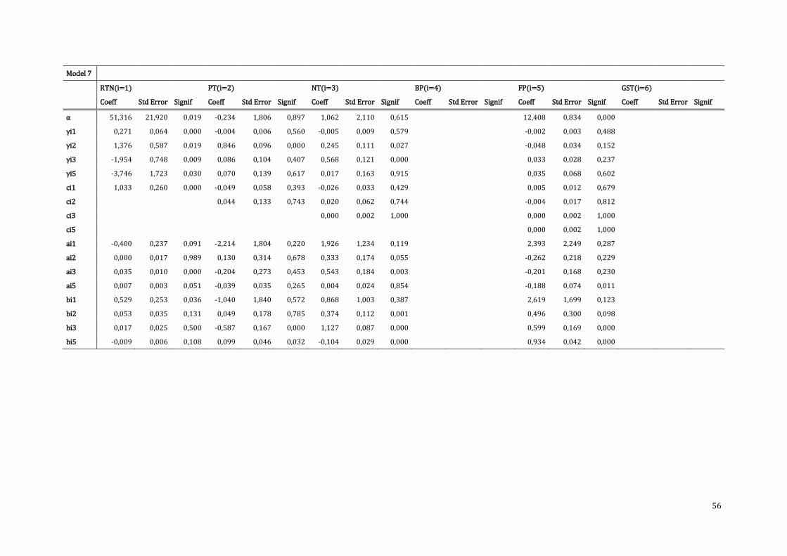
56

Model 7

RTN(i=1)

PT(i=2)

NT(i=3)

BP(i=4)

FP(i=5)

GST(i=6)

Coeff Std Error Signif Coeff Std Error Signif Coeff Std Error Signif Coeff Std Error Signif Coeff Std Error Signif Coeff Std Error Signif

α 51,316 21,920 0,019 -0,234 1,806 0,897 1,062 2,110 0,615

12,408 0,834 0,000

γi1 0,271 0,064 0,000 -0,004 0,006 0,560 -0,005 0,009 0,579

-0,002 0,003 0,488

γi2 1,376 0,587 0,019 0,846 0,096 0,000 0,245 0,111 0,027

-0,048 0,034 0,152

γi3 -1,954 0,748 0,009 0,086 0,104 0,407 0,568 0,121 0,000

0,033 0,028 0,237

γi5 -3,746 1,723 0,030 0,070 0,139 0,617 0,017 0,163 0,915

0,035 0,068 0,602

ci1 1,033 0,260 0,000 -0,049 0,058 0,393 -0,026 0,033 0,429

0,005 0,012 0,679

ci2

0,044 0,133 0,743 0,020 0,062 0,744

-0,004 0,017 0,812

ci3

0,000 0,002 1,000

0,000 0,002 1,000

ci5

0,000 0,002 1,000

ai1 -0,400 0,237 0,091 -2,214 1,804 0,220 1,926 1,234 0,119

2,393 2,249 0,287

ai2 0,000 0,017 0,989 0,130 0,314 0,678 0,333 0,174 0,055

-0,262 0,218 0,229

ai3 0,035 0,010 0,000 -0,204 0,273 0,453 0,543 0,184 0,003

-0,201 0,168 0,230

ai5 0,007 0,003 0,051 -0,039 0,035 0,265 0,004 0,024 0,854

-0,188 0,074 0,011

bi1 0,529 0,253 0,036 -1,040 1,840 0,572 0,868 1,003 0,387

2,619 1,699 0,123

bi2 0,053 0,035 0,131 0,049 0,178 0,785 0,374 0,112 0,001

0,496 0,300 0,098

bi3 0,017 0,025 0,500 -0,587 0,167 0,000 1,127 0,087 0,000

0,599 0,169 0,000

bi5 -0,009 0,006 0,108 0,099 0,046 0,032 -0,104 0,029 0,000

0,934 0,042 0,000

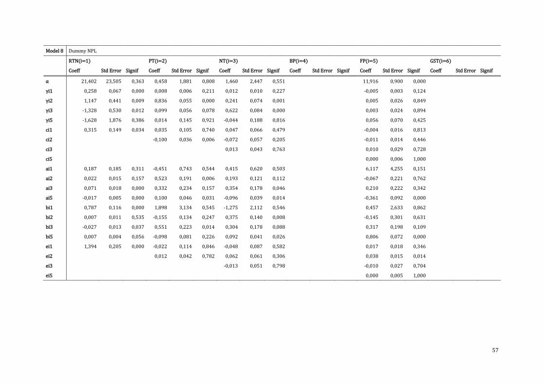
57

Model 8 Dummy NPL

RTN(i=1)

PT(i=2)

NT(i=3)

BP(i=4)

FP(i=5)

GST(i=6)

Coeff Std Error Signif Coeff Std Error Signif Coeff Std Error Signif Coeff Std Error Signif Coeff Std Error Signif Coeff Std Error Signif

α 21,402 23,505 0,363 0,458 1,881 0,808 1,460 2,447 0,551

11,916 0,900 0,000

γi1 0,258 0,067 0,000 0,008 0,006 0,211 0,012 0,010 0,227

-0,005 0,003 0,124

γi2 1,147 0,441 0,009 0,836 0,055 0,000 0,241 0,074 0,001

0,005 0,026 0,849

γi3 -1,328 0,530 0,012 0,099 0,056 0,078 0,622 0,084 0,000

0,003 0,024 0,894

γi5 -1,628 1,876 0,386 0,014 0,145 0,921 -0,044 0,188 0,816

0,056 0,070 0,425

ci1 0,315 0,149 0,034 0,035 0,105 0,740 0,047 0,066 0,479

-0,004 0,016 0,813

ci2

-0,100 0,036 0,006 -0,072 0,057 0,205

-0,011 0,014 0,446

ci3

0,013 0,043 0,763

0,010 0,029 0,728

ci5

0,000 0,006 1,000

ai1 0,187 0,185 0,311 -0,451 0,743 0,544 0,415 0,620 0,503

6,117 4,255 0,151

ai2 0,022 0,015 0,157 0,523 0,191 0,006 0,193 0,121 0,112

-0,067 0,221 0,762

ai3 0,071 0,018 0,000 0,332 0,234 0,157 0,354 0,178 0,046

0,210 0,222 0,342

ai5 -0,017 0,005 0,000 0,100 0,046 0,031 -0,096 0,039 0,014

-0,361 0,092 0,000

bi1 0,787 0,116 0,000 1,898 3,134 0,545 -1,275 2,112 0,546

0,457 2,633 0,862

bi2 0,007 0,011 0,535 -0,155 0,134 0,247 0,375 0,140 0,008

-0,145 0,301 0,631

bi3 -0,027 0,013 0,037 0,551 0,223 0,014 0,304 0,178 0,088

0,317 0,198 0,109

bi5 0,007 0,004 0,056 -0,098 0,081 0,226 0,092 0,041 0,026

0,806 0,072 0,000

ei1 1,394 0,205 0,000 -0,022 0,114 0,846 -0,048 0,087 0,582

0,017 0,018 0,346

ei2

0,012 0,042 0,782 0,062 0,061 0,306

0,038 0,015 0,014

ei3

-0,013 0,051 0,798

-0,010 0,027 0,704

ei5

0,000 0,005 1,000

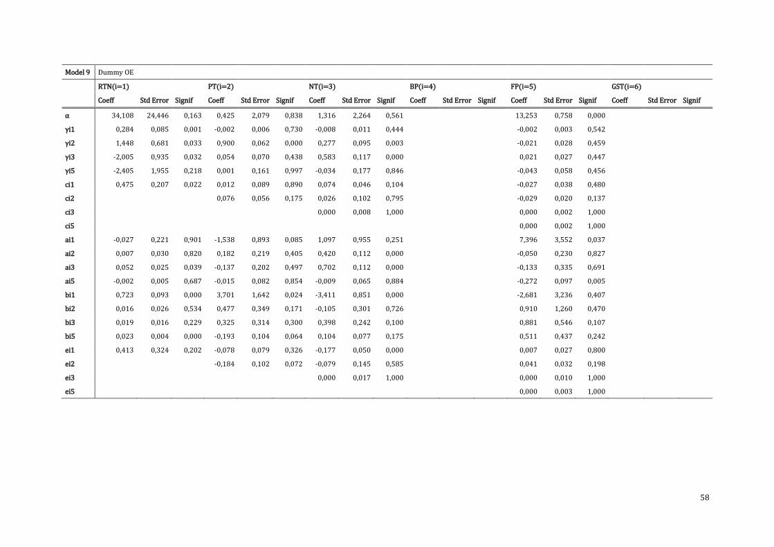
58

Model 9 Dummy OE

RTN(i=1)

PT(i=2)

NT(i=3)

BP(i=4)

FP(i=5)

GST(i=6)

Coeff Std Error Signif Coeff Std Error Signif Coeff Std Error Signif Coeff Std Error Signif Coeff Std Error Signif Coeff Std Error Signif

α 34,108 24,446 0,163 0,425 2,079 0,838 1,316 2,264 0,561

13,253 0,758 0,000

γi1 0,284 0,085 0,001 -0,002 0,006 0,730 -0,008 0,011 0,444

-0,002 0,003 0,542

γi2 1,448 0,681 0,033 0,900 0,062 0,000 0,277 0,095 0,003

-0,021 0,028 0,459

γi3 -2,005 0,935 0,032 0,054 0,070 0,438 0,583 0,117 0,000

0,021 0,027 0,447

γi5 -2,405 1,955 0,218 0,001 0,161 0,997 -0,034 0,177 0,846

-0,043 0,058 0,456

ci1 0,475 0,207 0,022 0,012 0,089 0,890 0,074 0,046 0,104

-0,027 0,038 0,480

ci2

0,076 0,056 0,175 0,026 0,102 0,795

-0,029 0,020 0,137

ci3

0,000 0,008 1,000

0,000 0,002 1,000

ci5

0,000 0,002 1,000

ai1 -0,027 0,221 0,901 -1,538 0,893 0,085 1,097 0,955 0,251

7,396 3,552 0,037

ai2 0,007 0,030 0,820 0,182 0,219 0,405 0,420 0,112 0,000

-0,050 0,230 0,827

ai3 0,052 0,025 0,039 -0,137 0,202 0,497 0,702 0,112 0,000

-0,133 0,335 0,691

ai5 -0,002 0,005 0,687 -0,015 0,082 0,854 -0,009 0,065 0,884

-0,272 0,097 0,005

bi1 0,723 0,093 0,000 3,701 1,642 0,024 -3,411 0,851 0,000

-2,681 3,236 0,407

bi2 0,016 0,026 0,534 0,477 0,349 0,171 -0,105 0,301 0,726

0,910 1,260 0,470

bi3 0,019 0,016 0,229 0,325 0,314 0,300 0,398 0,242 0,100

0,881 0,546 0,107

bi5 0,023 0,004 0,000 -0,193 0,104 0,064 0,104 0,077 0,175

0,511 0,437 0,242

ei1 0,413 0,324 0,202 -0,078 0,079 0,326 -0,177 0,050 0,000

0,007 0,027 0,800

ei2

-0,184 0,102 0,072 -0,079 0,145 0,585

0,041 0,032 0,198

ei3

0,000 0,017 1,000

0,000 0,010 1,000

ei5

0,000 0,003 1,000

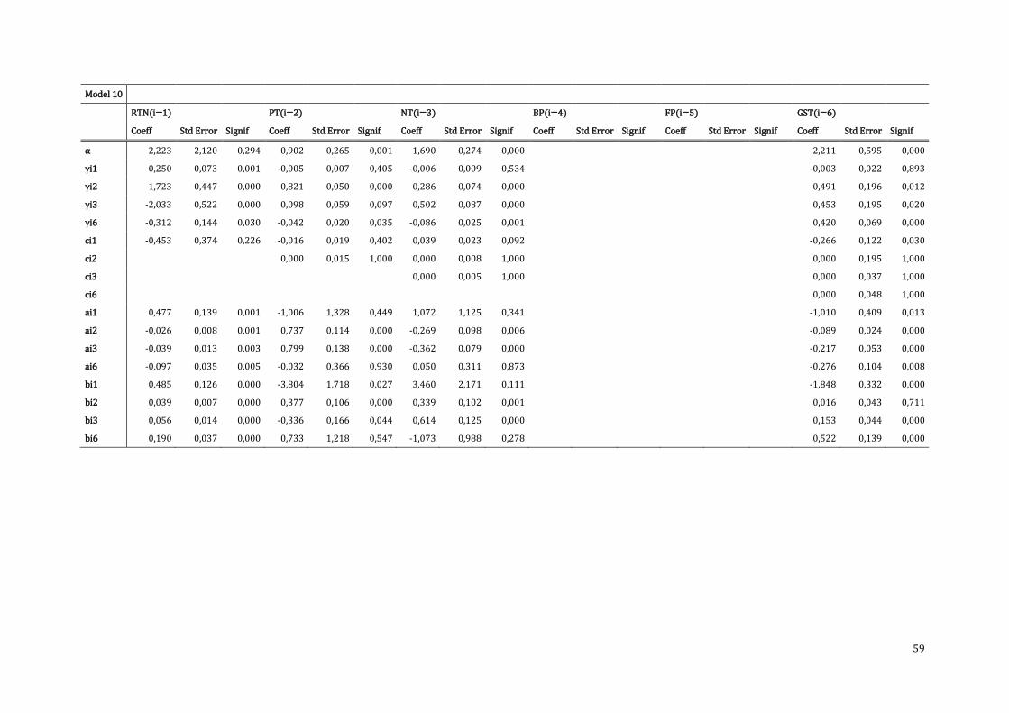
59

Model 10

RTN(i=1)

PT(i=2)

NT(i=3)

BP(i=4)

FP(i=5)

GST(i=6)

Coeff Std Error Signif Coeff Std Error Signif Coeff Std Error Signif Coeff Std Error Signif Coeff Std Error Signif Coeff Std Error Signif

α 2,223 2,120 0,294 0,902 0,265 0,001 1,690 0,274 0,000

2,211 0,595 0,000

γi1 0,250 0,073 0,001 -0,005 0,007 0,405 -0,006 0,009 0,534

-0,003 0,022 0,893

γi2 1,723 0,447 0,000 0,821 0,050 0,000 0,286 0,074 0,000

-0,491 0,196 0,012

γi3 -2,033 0,522 0,000 0,098 0,059 0,097 0,502 0,087 0,000

0,453 0,195 0,020

γi6 -0,312 0,144 0,030 -0,042 0,020 0,035 -0,086 0,025 0,001

0,420 0,069 0,000

ci1 -0,453 0,374 0,226 -0,016 0,019 0,402 0,039 0,023 0,092

-0,266 0,122 0,030

ci2

0,000 0,015 1,000 0,000 0,008 1,000

0,000 0,195 1,000

ci3

0,000 0,005 1,000

0,000 0,037 1,000

ci6

0,000 0,048 1,000

ai1 0,477 0,139 0,001 -1,006 1,328 0,449 1,072 1,125 0,341

-1,010 0,409 0,013

ai2 -0,026 0,008 0,001 0,737 0,114 0,000 -0,269 0,098 0,006

-0,089 0,024 0,000

ai3 -0,039 0,013 0,003 0,799 0,138 0,000 -0,362 0,079 0,000

-0,217 0,053 0,000

ai6 -0,097 0,035 0,005 -0,032 0,366 0,930 0,050 0,311 0,873

-0,276 0,104 0,008

bi1 0,485 0,126 0,000 -3,804 1,718 0,027 3,460 2,171 0,111

-1,848 0,332 0,000

bi2 0,039 0,007 0,000 0,377 0,106 0,000 0,339 0,102 0,001

0,016 0,043 0,711

bi3 0,056 0,014 0,000 -0,336 0,166 0,044 0,614 0,125 0,000

0,153 0,044 0,000

bi6 0,190 0,037 0,000 0,733 1,218 0,547 -1,073 0,988 0,278

0,522 0,139 0,000

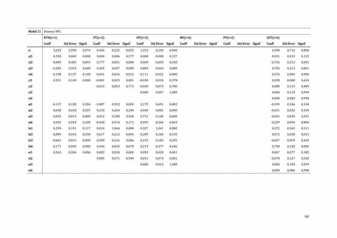
60

Model 11 Dummy NPL

RTN(i=1)

PT(i=2)

NT(i=3)

BP(i=4)

FP(i=5)

GST(i=6)

Coeff Std Error Signif Coeff Std Error Signif Coeff Std Error Signif Coeff Std Error Signif Coeff Std Error Signif Coeff Std Error Signif

α 3,625 2,030 0,074 0,426 0,222 0,055 1,253 0,240 0,000

2,498 0,716 0,000

γi1 0,358 0,069 0,000 0,004 0,006 0,577 0,008 0,008 0,327

0,031 0,019 0,115

γi2 -0,089 0,485 0,854 0,777 0,051 0,000 0,069 0,059 0,240

-0,726 0,213 0,001

γi3 -0,285 0,554 0,608 0,205 0,057 0,000 0,804 0,064 0,000

0,703 0,213 0,001

γi6 -0,198 0,137 0,148 -0,041 0,016 0,012 -0,111 0,022 0,000

0,376 0,084 0,000

ci1 0,591 0,169 0,000 -0,081 0,025 0,001 -0,030 0,034 0,378

0,038 0,080 0,634

ci2

-0,015 0,053 0,773 -0,020 0,073 0,780

0,080 0,115 0,489

ci3

0,000 0,007 1,000

0,000 0,110 0,999

ci6

0,000 0,083 0,998

ai1 -0,137 0,128 0,284 -2,887 0,952 0,002 2,175 0,691 0,002

-0,399 0,246 0,104

ai2 0,038 0,018 0,037 0,310 0,264 0,240 0,440 0,081 0,000

-0,051 0,032 0,109

ai3 0,055 0,013 0,000 0,012 0,298 0,968 0,731 0,100 0,000

-0,041 0,039 0,291

ai6 0,039 0,024 0,100 -0,430 0,314 0,171 0,495 0,266 0,063

-0,259 0,094 0,006

bi1 0,299 0,191 0,117 8,814 1,064 0,000 -5,927 1,041 0,000

0,372 0,565 0,511

bi2 -0,009 0,016 0,550 0,617 0,212 0,004 -0,209 0,160 0,193

0,072 0,030 0,015

bi3 -0,063 0,015 0,000 0,599 0,216 0,006 0,155 0,183 0,395

-0,057 0,070 0,418

bi6 -0,177 0,043 0,000 0,346 0,833 0,678 0,219 0,477 0,646

0,758 0,158 0,000

ei1 0,563 0,204 0,006 0,082 0,020 0,000 0,093 0,028 0,001

0,067 0,077 0,385

ei2

0,005 0,071 0,949 0,031 0,074 0,681

-0,078 0,127 0,536

ei3

0,000 0,014 1,000

0,000 0,109 0,999

ei6

0,000 0,086 0,998

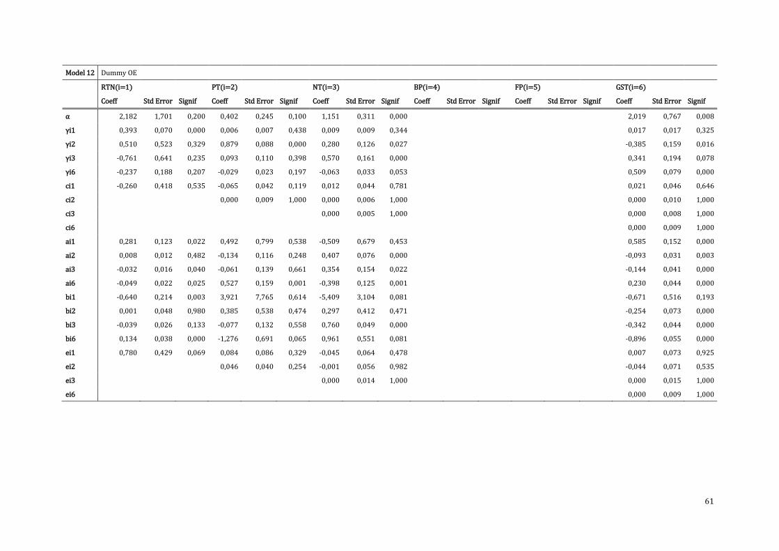
61

Model 12 Dummy OE

RTN(i=1)

PT(i=2)

NT(i=3)

BP(i=4)

FP(i=5)

GST(i=6)

Coeff Std Error Signif Coeff Std Error Signif Coeff Std Error Signif Coeff Std Error Signif Coeff Std Error Signif Coeff Std Error Signif

α 2,182 1,701 0,200 0,402 0,245 0,100 1,151 0,311 0,000

2,019 0,767 0,008

γi1 0,393 0,070 0,000 0,006 0,007 0,438 0,009 0,009 0,344

0,017 0,017 0,325

γi2 0,510 0,523 0,329 0,879 0,088 0,000 0,280 0,126 0,027

-0,385 0,159 0,016

γi3 -0,761 0,641 0,235 0,093 0,110 0,398 0,570 0,161 0,000

0,341 0,194 0,078

γi6 -0,237 0,188 0,207 -0,029 0,023 0,197 -0,063 0,033 0,053

0,509 0,079 0,000

ci1 -0,260 0,418 0,535 -0,065 0,042 0,119 0,012 0,044 0,781

0,021 0,046 0,646

ci2

0,000 0,009 1,000 0,000 0,006 1,000

0,000 0,010 1,000

ci3

0,000 0,005 1,000

0,000 0,008 1,000

ci6

0,000 0,009 1,000

ai1 0,281 0,123 0,022 0,492 0,799 0,538 -0,509 0,679 0,453

0,585 0,152 0,000

ai2 0,008 0,012 0,482 -0,134 0,116 0,248 0,407 0,076 0,000

-0,093 0,031 0,003

ai3 -0,032 0,016 0,040 -0,061 0,139 0,661 0,354 0,154 0,022

-0,144 0,041 0,000

ai6 -0,049 0,022 0,025 0,527 0,159 0,001 -0,398 0,125 0,001

0,230 0,044 0,000

bi1 -0,640 0,214 0,003 3,921 7,765 0,614 -5,409 3,104 0,081

-0,671 0,516 0,193

bi2 0,001 0,048 0,980 0,385 0,538 0,474 0,297 0,412 0,471

-0,254 0,073 0,000

bi3 -0,039 0,026 0,133 -0,077 0,132 0,558 0,760 0,049 0,000

-0,342 0,044 0,000

bi6 0,134 0,038 0,000 -1,276 0,691 0,065 0,961 0,551 0,081

-0,896 0,055 0,000

ei1 0,780 0,429 0,069 0,084 0,086 0,329 -0,045 0,064 0,478

0,007 0,073 0,925

ei2

0,046 0,040 0,254 -0,001 0,056 0,982

-0,044 0,071 0,535

ei3

0,000 0,014 1,000

0,000 0,015 1,000

ei6

0,000 0,009 1,000

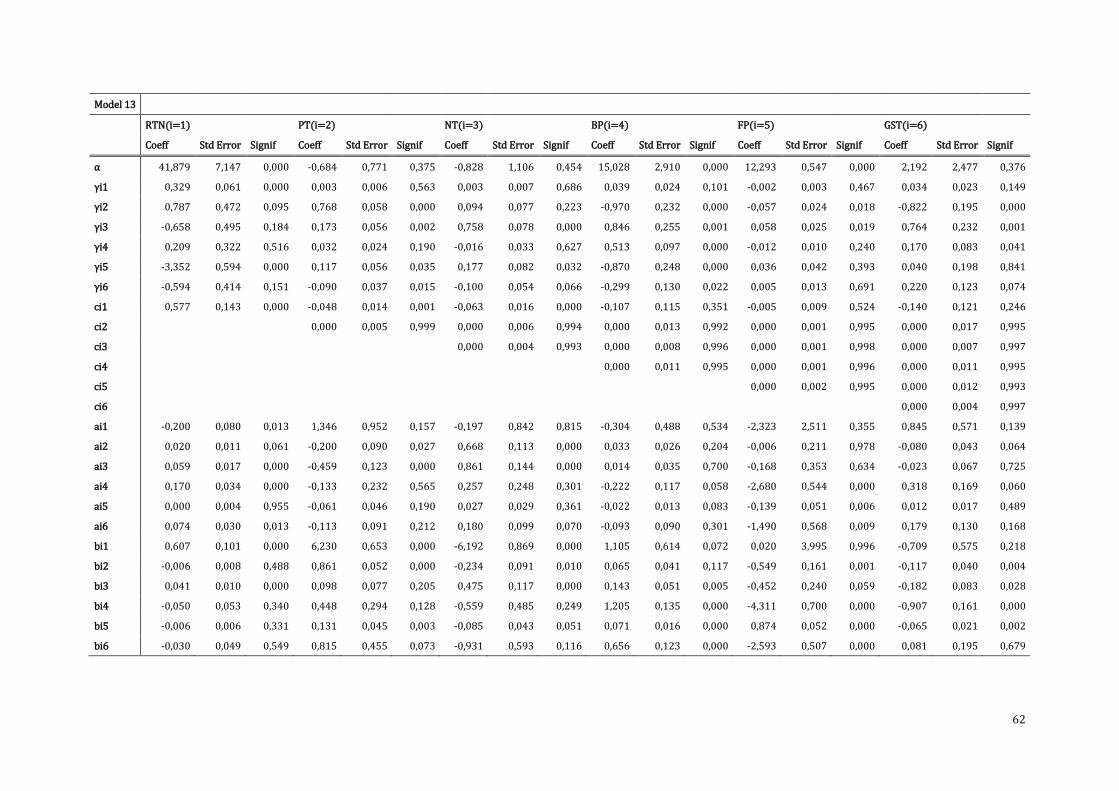
62

Model 13

RTN(i=1)

PT(i=2)

NT(i=3)

BP(i=4)

FP(i=5)

GST(i=6)

Coeff Std Error Signif Coeff Std Error Signif Coeff Std Error Signif Coeff Std Error Signif Coeff Std Error Signif Coeff Std Error Signif

α 41,879 7,147 0,000 -0,684 0,771 0,375 -0,828 1,106 0,454 15,028 2,910 0,000 12,293 0,547 0,000 2,192 2,477 0,376

γi1 0,329 0,061 0,000 0,003 0,006 0,563 0,003 0,007 0,686 0,039 0,024 0,101 -0,002 0,003 0,467 0,034 0,023 0,149

γi2 0,787 0,472 0,095 0,768 0,058 0,000 0,094 0,077 0,223 -0,970 0,232 0,000 -0,057 0,024 0,018 -0,822 0,195 0,000

γi3 -0,658 0,495 0,184 0,173 0,056 0,002 0,758 0,078 0,000 0,846 0,255 0,001 0,058 0,025 0,019 0,764 0,232 0,001

γi4 0,209 0,322 0,516 0,032 0,024 0,190 -0,016 0,033 0,627 0,513 0,097 0,000 -0,012 0,010 0,240 0,170 0,083 0,041

γi5 -3,352 0,594 0,000 0,117 0,056 0,035 0,177 0,082 0,032 -0,870 0,248 0,000 0,036 0,042 0,393 0,040 0,198 0,841

γi6 -0,594 0,414 0,151 -0,090 0,037 0,015 -0,100 0,054 0,066 -0,299 0,130 0,022 0,005 0,013 0,691 0,220 0,123 0,074

ci1 0,577 0,143 0,000 -0,048 0,014 0,001 -0,063 0,016 0,000 -0,107 0,115 0,351 -0,005 0,009 0,524 -0,140 0,121 0,246

ci2

0,000 0,005 0,999 0,000 0,006 0,994 0,000 0,013 0,992 0,000 0,001 0,995 0,000 0,017 0,995

ci3

0,000 0,004 0,993 0,000 0,008 0,996 0,000 0,001 0,998 0,000 0,007 0,997

ci4

0,000 0,011 0,995 0,000 0,001 0,996 0,000 0,011 0,995

ci5

0,000 0,002 0,995 0,000 0,012 0,993

ci6

0,000 0,004 0,997

ai1 -0,200 0,080 0,013 1,346 0,952 0,157 -0,197 0,842 0,815 -0,304 0,488 0,534 -2,323 2,511 0,355 0,845 0,571 0,139

ai2 0,020 0,011 0,061 -0,200 0,090 0,027 0,668 0,113 0,000 0,033 0,026 0,204 -0,006 0,211 0,978 -0,080 0,043 0,064

ai3 0,059 0,017 0,000 -0,459 0,123 0,000 0,861 0,144 0,000 0,014 0,035 0,700 -0,168 0,353 0,634 -0,023 0,067 0,725

ai4 0,170 0,034 0,000 -0,133 0,232 0,565 0,257 0,248 0,301 -0,222 0,117 0,058 -2,680 0,544 0,000 0,318 0,169 0,060

ai5 0,000 0,004 0,955 -0,061 0,046 0,190 0,027 0,029 0,361 -0,022 0,013 0,083 -0,139 0,051 0,006 0,012 0,017 0,489

ai6 0,074 0,030 0,013 -0,113 0,091 0,212 0,180 0,099 0,070 -0,093 0,090 0,301 -1,490 0,568 0,009 0,179 0,130 0,168

bi1 0,607 0,101 0,000 6,230 0,653 0,000 -6,192 0,869 0,000 1,105 0,614 0,072 0,020 3,995 0,996 -0,709 0,575 0,218

bi2 -0,006 0,008 0,488 0,861 0,052 0,000 -0,234 0,091 0,010 0,065 0,041 0,117 -0,549 0,161 0,001 -0,117 0,040 0,004

bi3 0,041 0,010 0,000 0,098 0,077 0,205 0,475 0,117 0,000 0,143 0,051 0,005 -0,452 0,240 0,059 -0,182 0,083 0,028

bi4 -0,050 0,053 0,340 0,448 0,294 0,128 -0,559 0,485 0,249 1,205 0,135 0,000 -4,311 0,700 0,000 -0,907 0,161 0,000

bi5 -0,006 0,006 0,331 0,131 0,045 0,003 -0,085 0,043 0,051 0,071 0,016 0,000 0,874 0,052 0,000 -0,065 0,021 0,002

bi6 -0,030 0,049 0,549 0,815 0,455 0,073 -0,931 0,593 0,116 0,656 0,123 0,000 -2,593 0,507 0,000 0,081 0,195 0,679

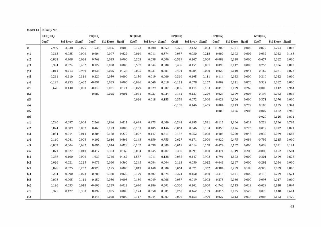
63

Model 14 Dummy NPL

RTN(i=1)

PT(i=2)

NT(i=3)

BP(i=4)

FP(i=5)

GST(i=6)

Coeff Std Error Signif Coeff Std Error Signif Coeff Std Error Signif Coeff Std Error Signif Coeff Std Error Signif Coeff Std Error Signif

α 7,939 3,538 0,025 -1,536 0,886 0,083 0,123 0,208 0,553 6,376 2,122 0,003 11,289 0,301 0,000 0,879 0,294 0,003

γi1 0,313 0,085 0,000 0,004 0,007 0,622 0,010 0,011 0,374 0,037 0,030 0,218 0,002 0,003 0,602 0,032 0,023 0,163

γi2 -0,863 0,408 0,034 0,762 0,045 0,000 0,203 0,038 0,000 -0,519 0,107 0,000 -0,082 0,018 0,000 -0,477 0,062 0,000

γi3 0,394 0,524 0,452 0,122 0,030 0,000 0,557 0,044 0,000 0,486 0,151 0,001 0,093 0,017 0,000 0,256 0,086 0,003

γi4 0,011 0,213 0,959 0,038 0,025 0,128 -0,005 0,031 0,881 0,494 0,084 0,000 -0,020 0,010 0,044 0,162 0,071 0,023

γi5 -0,211 0,210 0,314 0,220 0,059 0,000 0,150 0,019 0,000 -0,310 0,195 0,111 0,114 0,023 0,000 0,210 0,022 0,000

γi6 -0,199 0,253 0,432 -0,097 0,035 0,006 -0,096 0,040 0,018 -0,111 0,078 0,157 0,002 0,011 0,873 0,312 0,082 0,000

ci1 0,678 0,140 0,000 -0,043 0,031 0,171 -0,079 0,029 0,007 -0,085 0,114 0,454 -0,010 0,009 0,269 0,005 0,112 0,964

ci2

-0,087 0,025 0,001 -0,061 0,027 0,024 -0,132 0,127 0,299 -0,025 0,009 0,003 -0,196 0,083 0,018

ci3

0,026 0,018 0,155 0,376 0,072 0,000 -0,028 0,006 0,000 0,371 0,070 0,000

ci4

-0,109 0,146 0,455 0,004 0,013 0,772 0,100 0,105 0,341

ci5

0,000 0,006 0,983 0,007 0,162 0,965

ci6

-0,020 0,126 0,871

ai1 0,280 0,097 0,004 2,269 0,896 0,011 -3,649 0,873 0,000 -0,241 0,395 0,541 -8,115 3,306 0,014 0,229 0,766 0,765

ai2 0,024 0,009 0,007 0,463 0,123 0,000 -0,153 0,105 0,146 -0,061 0,046 0,184 0,050 0,176 0,776 0,012 0,072 0,871

ai3 0,034 0,014 0,014 0,204 0,188 0,279 0,097 0,147 0,511 -0,137 0,052 0,008 -0,405 0,200 0,043 0,032 0,079 0,687

ai4 0,110 0,041 0,008 0,102 0,616 0,868 -0,143 0,459 0,755 0,627 0,171 0,000 -0,820 0,475 0,084 -0,795 0,215 0,000

ai5 -0,007 0,004 0,087 0,096 0,044 0,028 -0,102 0,039 0,009 -0,019 0,014 0,168 -0,474 0,102 0,000 0,033 0,021 0,124

ai6 0,071 0,027 0,010 -0,417 0,303 0,169 0,004 0,245 0,987 0,385 0,091 0,000 -0,371 0,349 0,288 -0,083 0,152 0,584

bi1 0,386 0,100 0,000 1,030 0,746 0,167 1,537 1,011 0,128 0,055 0,447 0,902 6,791 1,802 0,000 -0,201 0,409 0,623

bi2 0,026 0,021 0,225 0,073 0,080 0,360 0,245 0,084 0,004 0,113 0,050 0,022 -0,643 0,167 0,000 -0,292 0,054 0,000

bi3 0,028 0,025 0,252 -0,923 0,125 0,000 0,813 0,140 0,000 0,064 0,071 0,362 -0,384 0,289 0,183 -0,328 0,069 0,000

bi4 0,204 0,090 0,023 -0,788 0,338 0,020 0,129 0,307 0,674 -0,324 0,150 0,030 -3,415 0,821 0,000 -0,118 0,209 0,574

bi5 0,008 0,005 0,114 -0,152 0,050 0,003 0,130 0,049 0,008 -0,057 0,019 0,002 -0,278 0,066 0,000 0,093 0,017 0,000

bi6 0,126 0,053 0,018 -0,603 0,239 0,012 0,640 0,186 0,001 -0,360 0,101 0,000 -1,748 0,745 0,019 -0,029 0,148 0,847

ei1 0,375 0,427 0,380 0,092 0,035 0,008 0,174 0,050 0,001 0,260 0,162 0,109 -0,016 0,025 0,529 0,073 0,140 0,604

ei2

0,146 0,028 0,000 0,117 0,044 0,007 0,000 0,153 0,999 -0,027 0,013 0,038 0,083 0,103 0,420

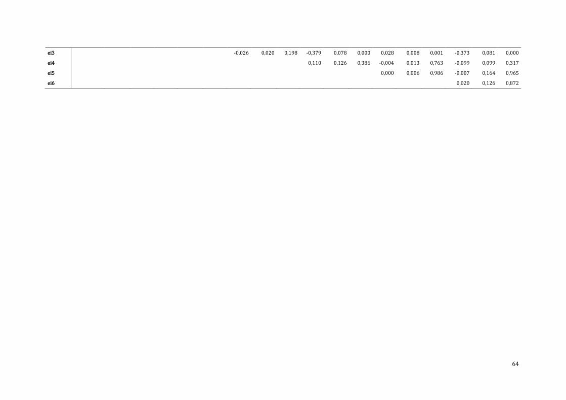
64

ei3

-0,026 0,020 0,198 -0,379 0,078 0,000 0,028 0,008 0,001 -0,373 0,081 0,000

ei4

0,110 0,126 0,386 -0,004 0,013 0,763 -0,099 0,099 0,317

ei5

0,000 0,006 0,986 -0,007 0,164 0,965

ei6

0,020 0,126 0,872

65

Model 15 Dummy OE

RTN(i=1)

PT(i=2)

NT(i=3)

BP(i=4)

FP(i=5)

GST(i=6)

Coeff Std Error Signif Coeff Std Error Signif Coeff Std Error Signif Coeff Std Error Signif Coeff Std Error Signif Coeff Std Error Signif

α 35,066 21,512 0,103 -1,358 3,070 0,658 -1,883 3,755 0,616 23,314 8,785 0,008 14,302 1,326 0,000 7,377 9,553 0,440

γi1 0,306 0,088 0,000 0,009 0,008 0,279 0,013 0,011 0,216 0,063 0,051 0,216 -0,001 0,003 0,660 0,054 0,034 0,108

γi2 0,421 0,543 0,438 0,889 0,083 0,000 0,258 0,092 0,005 -0,780 0,242 0,001 -0,056 0,031 0,070 -0,581 0,175 0,001

γi3 -0,986 0,578 0,088 0,030 0,108 0,783 0,579 0,124 0,000 0,764 0,238 0,001 0,065 0,030 0,028 0,571 0,216 0,008

γi4 0,112 0,244 0,644 0,043 0,028 0,128 0,048 0,040 0,229 0,478 0,145 0,001 -0,044 0,011 0,000 0,093 0,097 0,336

γi5 -2,255 1,669 0,177 0,180 0,259 0,486 0,264 0,321 0,410 -1,583 0,699 0,024 -0,125 0,097 0,197 -0,400 0,799 0,616

γi6 -0,910 0,346 0,009 -0,121 0,035 0,001 -0,195 0,052 0,000 -0,337 0,185 0,069 0,030 0,011 0,010 0,251 0,127 0,047

ci1 -0,328 0,195 0,091 0,000 0,055 0,999 -0,013 0,074 0,862 -0,035 0,138 0,803 0,029 0,019 0,124 0,020 0,169 0,904

ci2

0,031 0,022 0,162 0,038 0,025 0,126 0,180 0,161 0,263 0,000 0,015 0,976 0,319 0,134 0,017

ci3

0,000 0,004 1,000 0,000 0,025 1,000 0,000 0,003 1,000 0,000 0,052 1,000

ci4

0,000 0,021 1,000 0,000 0,003 1,000 0,000 0,043 1,000

ci5

0,000 0,003 1,000 0,000 0,020 1,000

ci6

0,000 0,016 1,000

ai1 -0,123 0,106 0,244 1,837 1,042 0,078 -2,008 1,293 0,120 -0,615 0,355 0,083 -0,211 2,681 0,937 0,338 0,399 0,398

ai2 0,034 0,016 0,031 0,148 0,144 0,302 0,261 0,127 0,040 -0,056 0,060 0,350 0,040 0,423 0,924 0,021 0,079 0,793

ai3 0,068 0,018 0,000 0,039 0,138 0,777 0,428 0,126 0,001 -0,132 0,063 0,036 0,285 0,364 0,434 0,109 0,087 0,211

ai4 0,165 0,069 0,017 0,351 0,503 0,485 -0,305 0,490 0,533 0,035 0,138 0,801 -2,385 1,331 0,073 -0,363 0,291 0,211

ai5 -0,015 0,005 0,005 0,035 0,033 0,291 -0,035 0,043 0,419 -0,032 0,017 0,068 -0,305 0,116 0,008 0,029 0,028 0,287

ai6 0,054 0,051 0,296 0,977 0,396 0,013 -0,836 0,309 0,007 -0,071 0,137 0,603 -0,048 1,323 0,971 0,290 0,238 0,223

bi1 0,677 0,100 0,000 -1,764 2,212 0,425 1,688 1,881 0,369 -1,390 0,591 0,019 -2,096 3,821 0,583 1,827 0,707 0,010

bi2 -0,008 0,015 0,608 0,719 0,123 0,000 -0,024 0,153 0,875 -0,183 0,105 0,080 0,950 0,503 0,059 0,161 0,153 0,294

bi3 -0,041 0,015 0,008 0,058 0,180 0,749 0,646 0,152 0,000 -0,285 0,095 0,003 0,215 0,914 0,814 0,203 0,141 0,149

bi4 -0,145 0,050 0,004 -1,117 0,977 0,253 1,333 0,610 0,029 -0,164 0,279 0,557 1,886 1,564 0,228 0,964 0,289 0,001

bi5 0,009 0,006 0,148 -0,212 0,062 0,001 0,243 0,056 0,000 0,031 0,043 0,464 0,544 0,165 0,001 -0,073 0,044 0,100

bi6 -0,086 0,041 0,035 -0,524 0,650 0,420 0,882 0,467 0,059 -0,055 0,224 0,805 1,275 1,010 0,207 0,628 0,247 0,011

ei1 1,555 0,393 0,000 0,000 0,074 0,998 0,010 0,075 0,893 0,063 0,175 0,717 -0,029 0,021 0,162 0,146 0,176 0,405

ei2

-0,079 0,040 0,048 -0,038 0,064 0,550 -0,371 0,222 0,095 0,009 0,024 0,721 -0,302 0,245 0,218

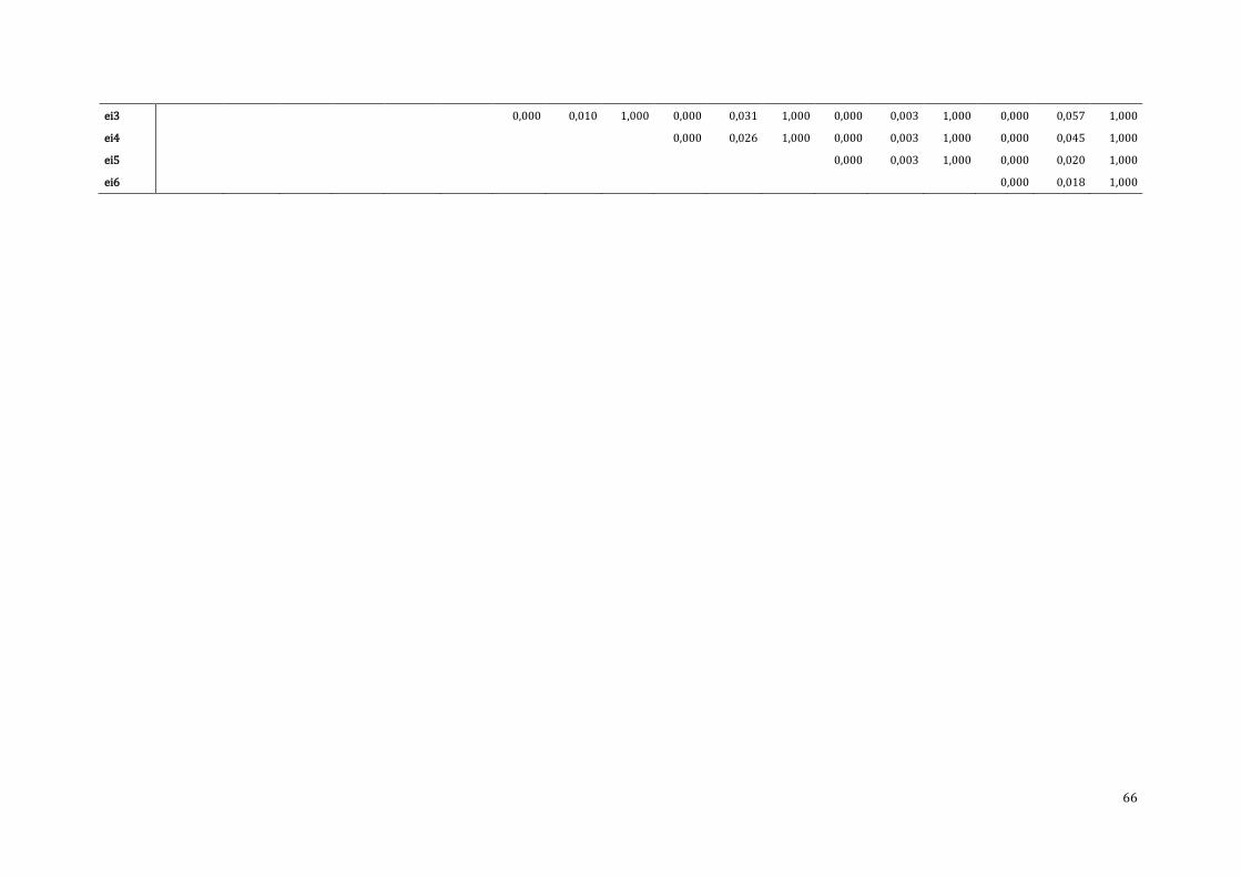
66

ei3

0,000 0,010 1,000 0,000 0,031 1,000 0,000 0,003 1,000 0,000 0,057 1,000

ei4

0,000 0,026 1,000 0,000 0,003 1,000 0,000 0,045 1,000

ei5

0,000 0,003 1,000 0,000 0,020 1,000

ei6

0,000 0,018 1,000

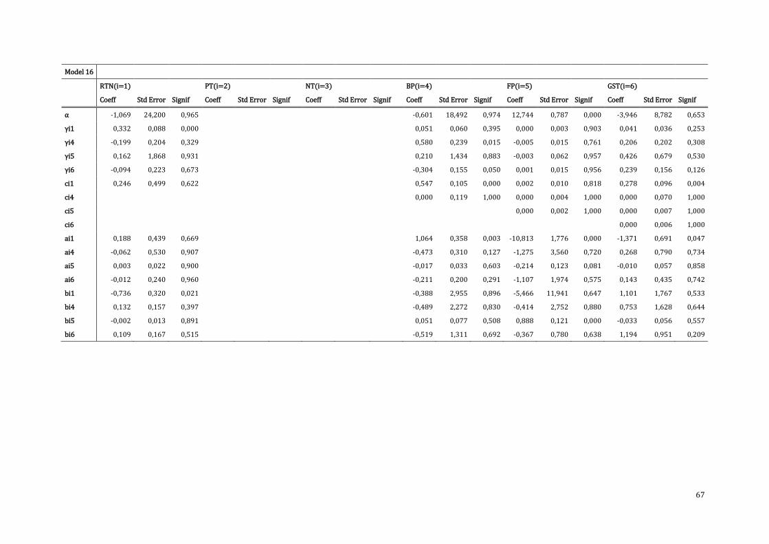
67

Model 16

RTN(i=1)

PT(i=2)

NT(i=3)

BP(i=4)

FP(i=5)

GST(i=6)

Coeff Std Error Signif Coeff Std Error Signif Coeff Std Error Signif Coeff Std Error Signif Coeff Std Error Signif Coeff Std Error Signif

α -1,069 24,200 0,965

-0,601 18,492 0,974 12,744 0,787 0,000 -3,946 8,782 0,653

γi1 0,332 0,088 0,000

0,051 0,060 0,395 0,000 0,003 0,903 0,041 0,036 0,253

γi4 -0,199 0,204 0,329

0,580 0,239 0,015 -0,005 0,015 0,761 0,206 0,202 0,308

γi5 0,162 1,868 0,931

0,210 1,434 0,883 -0,003 0,062 0,957 0,426 0,679 0,530

γi6 -0,094 0,223 0,673

-0,304 0,155 0,050 0,001 0,015 0,956 0,239 0,156 0,126

ci1 0,246 0,499 0,622

0,547 0,105 0,000 0,002 0,010 0,818 0,278 0,096 0,004

ci4

0,000 0,119 1,000 0,000 0,004 1,000 0,000 0,070 1,000

ci5

0,000 0,002 1,000 0,000 0,007 1,000

ci6

0,000 0,006 1,000

ai1 0,188 0,439 0,669

1,064 0,358 0,003 -10,813 1,776 0,000 -1,371 0,691 0,047

ai4 -0,062 0,530 0,907

-0,473 0,310 0,127 -1,275 3,560 0,720 0,268 0,790 0,734

ai5 0,003 0,022 0,900

-0,017 0,033 0,603 -0,214 0,123 0,081 -0,010 0,057 0,858

ai6 -0,012 0,240 0,960

-0,211 0,200 0,291 -1,107 1,974 0,575 0,143 0,435 0,742

bi1 -0,736 0,320 0,021

-0,388 2,955 0,896 -5,466 11,941 0,647 1,101 1,767 0,533

bi4 0,132 0,157 0,397

-0,489 2,272 0,830 -0,414 2,752 0,880 0,753 1,628 0,644

bi5 -0,002 0,013 0,891

0,051 0,077 0,508 0,888 0,121 0,000 -0,033 0,056 0,557

bi6 0,109 0,167 0,515

-0,519 1,311 0,692 -0,367 0,780 0,638 1,194 0,951 0,209

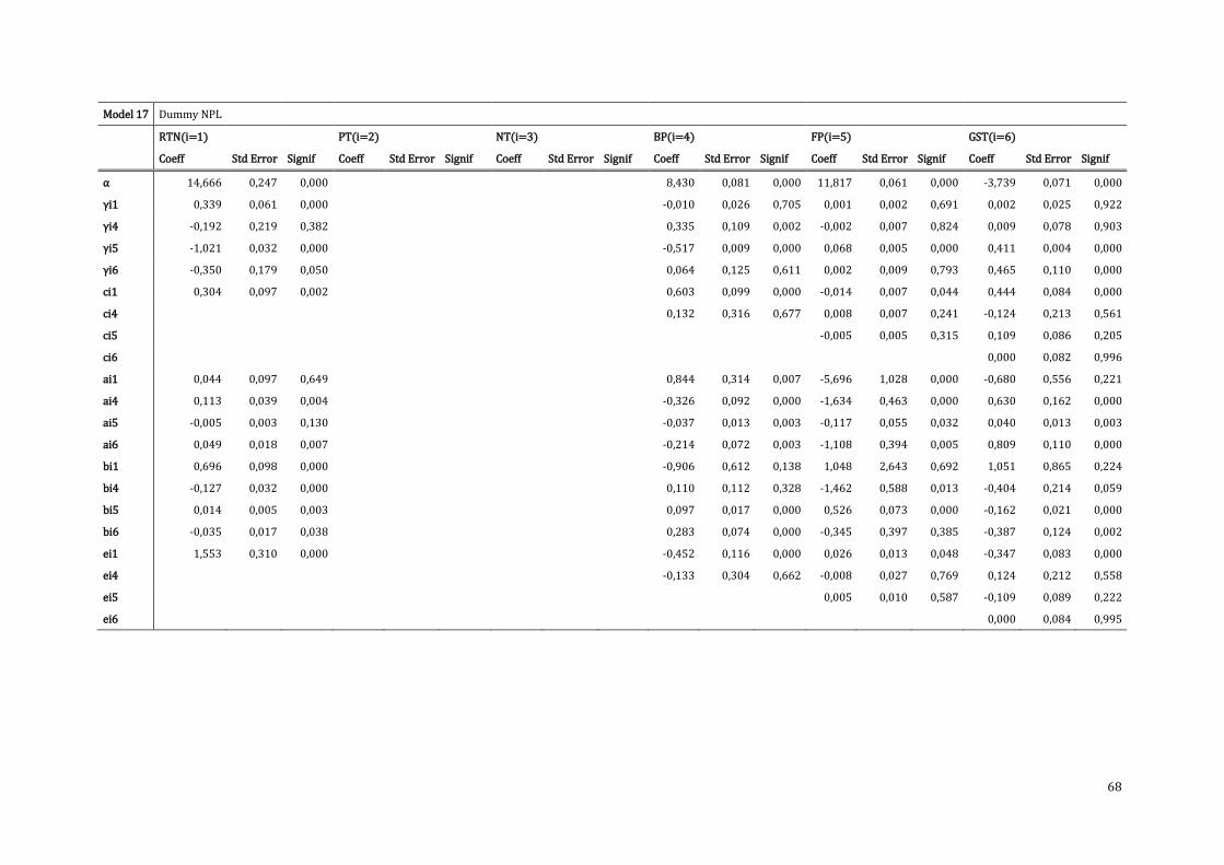
68

Model 17 Dummy NPL

RTN(i=1)

PT(i=2)

NT(i=3)

BP(i=4)

FP(i=5)

GST(i=6)

Coeff Std Error Signif Coeff Std Error Signif Coeff Std Error Signif Coeff Std Error Signif Coeff Std Error Signif Coeff Std Error Signif

α 14,666 0,247 0,000

8,430 0,081 0,000 11,817 0,061 0,000 -3,739 0,071 0,000

γi1 0,339 0,061 0,000

-0,010 0,026 0,705 0,001 0,002 0,691 0,002 0,025 0,922

γi4 -0,192 0,219 0,382

0,335 0,109 0,002 -0,002 0,007 0,824 0,009 0,078 0,903

γi5 -1,021 0,032 0,000

-0,517 0,009 0,000 0,068 0,005 0,000 0,411 0,004 0,000

γi6 -0,350 0,179 0,050

0,064 0,125 0,611 0,002 0,009 0,793 0,465 0,110 0,000

ci1 0,304 0,097 0,002

0,603 0,099 0,000 -0,014 0,007 0,044 0,444 0,084 0,000

ci4

0,132 0,316 0,677 0,008 0,007 0,241 -0,124 0,213 0,561

ci5

-0,005 0,005 0,315 0,109 0,086 0,205

ci6

0,000 0,082 0,996

ai1 0,044 0,097 0,649

0,844 0,314 0,007 -5,696 1,028 0,000 -0,680 0,556 0,221

ai4 0,113 0,039 0,004

-0,326 0,092 0,000 -1,634 0,463 0,000 0,630 0,162 0,000

ai5 -0,005 0,003 0,130

-0,037 0,013 0,003 -0,117 0,055 0,032 0,040 0,013 0,003

ai6 0,049 0,018 0,007

-0,214 0,072 0,003 -1,108 0,394 0,005 0,809 0,110 0,000

bi1 0,696 0,098 0,000

-0,906 0,612 0,138 1,048 2,643 0,692 1,051 0,865 0,224

bi4 -0,127 0,032 0,000

0,110 0,112 0,328 -1,462 0,588 0,013 -0,404 0,214 0,059

bi5 0,014 0,005 0,003

0,097 0,017 0,000 0,526 0,073 0,000 -0,162 0,021 0,000

bi6 -0,035 0,017 0,038

0,283 0,074 0,000 -0,345 0,397 0,385 -0,387 0,124 0,002

ei1 1,553 0,310 0,000

-0,452 0,116 0,000 0,026 0,013 0,048 -0,347 0,083 0,000

ei4

-0,133 0,304 0,662 -0,008 0,027 0,769 0,124 0,212 0,558

ei5

0,005 0,010 0,587 -0,109 0,089 0,222

ei6

0,000 0,084 0,995

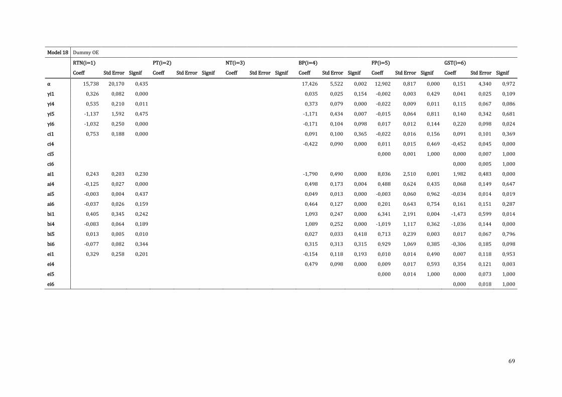
69

Model 18 Dummy OE

RTN(i=1)

PT(i=2)

NT(i=3)

BP(i=4)

FP(i=5)

GST(i=6)

Coeff Std Error Signif Coeff Std Error Signif Coeff Std Error Signif Coeff Std Error Signif Coeff Std Error Signif Coeff Std Error Signif

α 15,738 20,170 0,435

17,426 5,522 0,002 12,902 0,817 0,000 0,151 4,340 0,972

γi1 0,326 0,082 0,000

0,035 0,025 0,154 -0,002 0,003 0,429 0,041 0,025 0,109

γi4 0,535 0,210 0,011

0,373 0,079 0,000 -0,022 0,009 0,011 0,115 0,067 0,086

γi5 -1,137 1,592 0,475

-1,171 0,434 0,007 -0,015 0,064 0,811 0,140 0,342 0,681

γi6 -1,032 0,250 0,000

-0,171 0,104 0,098 0,017 0,012 0,144 0,220 0,098 0,024

ci1 0,753 0,188 0,000

0,091 0,100 0,365 -0,022 0,016 0,156 0,091 0,101 0,369

ci4

-0,422 0,090 0,000 0,011 0,015 0,469 -0,452 0,045 0,000

ci5

0,000 0,001 1,000 0,000 0,007 1,000

ci6

0,000 0,005 1,000

ai1 0,243 0,203 0,230

-1,790 0,490 0,000 8,036 2,510 0,001 1,982 0,483 0,000

ai4 -0,125 0,027 0,000

0,498 0,173 0,004 0,488 0,624 0,435 0,068 0,149 0,647

ai5 -0,003 0,004 0,437

0,049 0,013 0,000 -0,003 0,060 0,962 -0,034 0,014 0,019

ai6 -0,037 0,026 0,159

0,464 0,127 0,000 0,201 0,643 0,754 0,161 0,151 0,287

bi1 0,405 0,345 0,242

1,093 0,247 0,000 6,341 2,191 0,004 -1,473 0,599 0,014

bi4 -0,083 0,064 0,189

1,089 0,252 0,000 -1,019 1,117 0,362 -1,036 0,144 0,000

bi5 0,013 0,005 0,010

0,027 0,033 0,418 0,713 0,239 0,003 0,017 0,067 0,796

bi6 -0,077 0,082 0,344

0,315 0,313 0,315 0,929 1,069 0,385 -0,306 0,185 0,098

ei1 0,329 0,258 0,201

-0,154 0,118 0,193 0,010 0,014 0,490 0,007 0,118 0,953

ei4

0,479 0,098 0,000 0,009 0,017 0,593 0,354 0,121 0,003

ei5

0,000 0,014 1,000 0,000 0,073 1,000

ei6

0,000 0,018 1,000

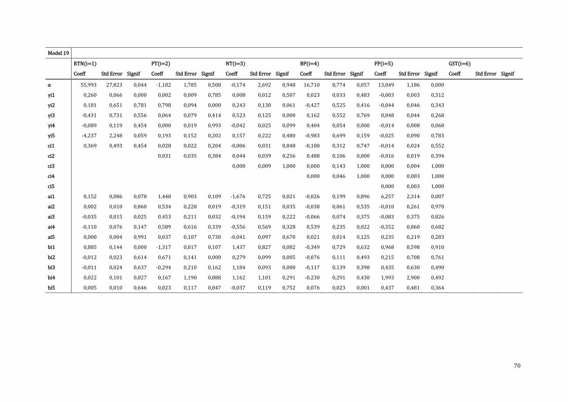
70

Model 19

RTN(i=1)

PT(i=2)

NT(i=3)

BP(i=4)

FP(i=5)

GST(i=6)

Coeff Std Error Signif Coeff Std Error Signif Coeff Std Error Signif Coeff Std Error Signif Coeff Std Error Signif Coeff Std Error Signif

α 55,993 27,823 0,044 -1,182 1,785 0,508 -0,174 2,692 0,948 16,710 8,774 0,057 13,049 1,186 0,000

γi1 0,260 0,066 0,000 0,002 0,009 0,785 0,008 0,012 0,507 0,023 0,033 0,483 -0,003 0,003 0,312

γi2 0,181 0,651 0,781 0,798 0,094 0,000 0,243 0,130 0,061 -0,427 0,525 0,416 -0,044 0,046 0,343

γi3 -0,431 0,731 0,556 0,064 0,079 0,414 0,523 0,125 0,000 0,162 0,552 0,769 0,048 0,044 0,268

γi4 -0,089 0,119 0,454 0,000 0,019 0,993 -0,042 0,025 0,099 0,404 0,054 0,000 -0,014 0,008 0,068

γi5 -4,237 2,248 0,059 0,193 0,152 0,202 0,157 0,222 0,480 -0,983 0,699 0,159 -0,025 0,090 0,783

ci1 0,369 0,493 0,454 0,028 0,022 0,204 -0,006 0,031 0,848 -0,100 0,312 0,747 -0,014 0,024 0,552

ci2

0,031 0,035 0,384 0,044 0,039 0,256 0,488 0,106 0,000 -0,016 0,019 0,394

ci3

0,000 0,009 1,000 0,000 0,143 1,000 0,000 0,004 1,000

ci4

0,000 0,046 1,000 0,000 0,003 1,000

ci5

0,000 0,003 1,000

ai1 0,152 0,086 0,078 1,448 0,903 0,109 -1,676 0,725 0,021 -0,026 0,199 0,896 6,257 2,314 0,007

ai2 0,002 0,010 0,860 0,534 0,228 0,019 -0,319 0,151 0,035 -0,038 0,061 0,535 -0,010 0,261 0,970

ai3 -0,035 0,015 0,025 0,453 0,211 0,032 -0,194 0,159 0,222 -0,066 0,074 0,375 -0,083 0,375 0,826

ai4 -0,110 0,076 0,147 0,589 0,616 0,339 -0,556 0,569 0,328 0,539 0,235 0,022 -0,352 0,860 0,682

ai5 0,000 0,004 0,991 0,037 0,107 0,730 -0,041 0,097 0,670 0,021 0,014 0,125 0,235 0,219 0,283

bi1 0,885 0,144 0,000 -1,317 0,817 0,107 1,437 0,827 0,082 -0,349 0,729 0,632 0,968 8,598 0,910

bi2 -0,012 0,023 0,614 0,671 0,141 0,000 0,279 0,099 0,005 -0,076 0,111 0,493 0,215 0,708 0,761

bi3 -0,011 0,024 0,637 -0,294 0,210 0,162 1,184 0,093 0,000 -0,117 0,139 0,398 0,435 0,630 0,490

bi4 0,022 0,101 0,827 0,167 1,190 0,888 1,162 1,101 0,291 -0,230 0,291 0,430 1,993 2,900 0,492

bi5 0,005 0,010 0,646 0,023 0,117 0,847 -0,037 0,119 0,752 0,076 0,023 0,001 0,437 0,481 0,364

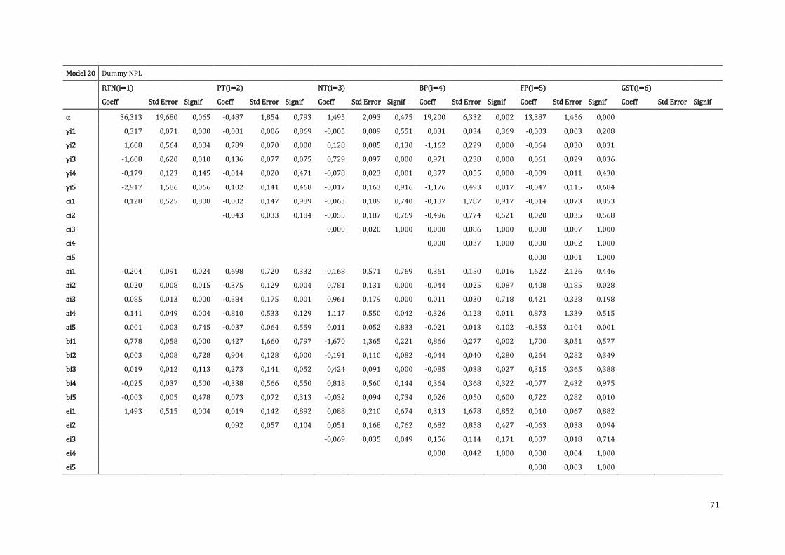
71

Model 20 Dummy NPL

RTN(i=1)

PT(i=2)

NT(i=3)

BP(i=4)

FP(i=5)

GST(i=6)

Coeff Std Error Signif Coeff Std Error Signif Coeff Std Error Signif Coeff Std Error Signif Coeff Std Error Signif Coeff Std Error Signif

α 36,313 19,680 0,065 -0,487 1,854 0,793 1,495 2,093 0,475 19,200 6,332 0,002 13,387 1,456 0,000

γi1 0,317 0,071 0,000 -0,001 0,006 0,869 -0,005 0,009 0,551 0,031 0,034 0,369 -0,003 0,003 0,208

γi2 1,608 0,564 0,004 0,789 0,070 0,000 0,128 0,085 0,130 -1,162 0,229 0,000 -0,064 0,030 0,031

γi3 -1,608 0,620 0,010 0,136 0,077 0,075 0,729 0,097 0,000 0,971 0,238 0,000 0,061 0,029 0,036

γi4 -0,179 0,123 0,145 -0,014 0,020 0,471 -0,078 0,023 0,001 0,377 0,055 0,000 -0,009 0,011 0,430

γi5 -2,917 1,586 0,066 0,102 0,141 0,468 -0,017 0,163 0,916 -1,176 0,493 0,017 -0,047 0,115 0,684

ci1 0,128 0,525 0,808 -0,002 0,147 0,989 -0,063 0,189 0,740 -0,187 1,787 0,917 -0,014 0,073 0,853

ci2

-0,043 0,033 0,184 -0,055 0,187 0,769 -0,496 0,774 0,521 0,020 0,035 0,568

ci3

0,000 0,020 1,000 0,000 0,086 1,000 0,000 0,007 1,000

ci4

0,000 0,037 1,000 0,000 0,002 1,000

ci5

0,000 0,001 1,000

ai1 -0,204 0,091 0,024 0,698 0,720 0,332 -0,168 0,571 0,769 0,361 0,150 0,016 1,622 2,126 0,446

ai2 0,020 0,008 0,015 -0,375 0,129 0,004 0,781 0,131 0,000 -0,044 0,025 0,087 0,408 0,185 0,028

ai3 0,085 0,013 0,000 -0,584 0,175 0,001 0,961 0,179 0,000 0,011 0,030 0,718 0,421 0,328 0,198

ai4 0,141 0,049 0,004 -0,810 0,533 0,129 1,117 0,550 0,042 -0,326 0,128 0,011 0,873 1,339 0,515

ai5 0,001 0,003 0,745 -0,037 0,064 0,559 0,011 0,052 0,833 -0,021 0,013 0,102 -0,353 0,104 0,001

bi1 0,778 0,058 0,000 0,427 1,660 0,797 -1,670 1,365 0,221 0,866 0,277 0,002 1,700 3,051 0,577

bi2 0,003 0,008 0,728 0,904 0,128 0,000 -0,191 0,110 0,082 -0,044 0,040 0,280 0,264 0,282 0,349

bi3 0,019 0,012 0,113 0,273 0,141 0,052 0,424 0,091 0,000 -0,085 0,038 0,027 0,315 0,365 0,388

bi4 -0,025 0,037 0,500 -0,338 0,566 0,550 0,818 0,560 0,144 0,364 0,368 0,322 -0,077 2,432 0,975

bi5 -0,003 0,005 0,478 0,073 0,072 0,313 -0,032 0,094 0,734 0,026 0,050 0,600 0,722 0,282 0,010

ei1 1,493 0,515 0,004 0,019 0,142 0,892 0,088 0,210 0,674 0,313 1,678 0,852 0,010 0,067 0,882

ei2

0,092 0,057 0,104 0,051 0,168 0,762 0,682 0,858 0,427 -0,063 0,038 0,094

ei3

-0,069 0,035 0,049 0,156 0,114 0,171 0,007 0,018 0,714

ei4

0,000 0,042 1,000 0,000 0,004 1,000

ei5

0,000 0,003 1,000

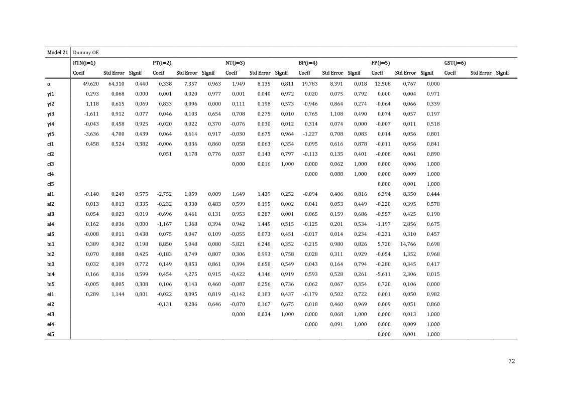
72

Model 21 Dummy OE

RTN(i=1)

PT(i=2)

NT(i=3)

BP(i=4)

FP(i=5)

GST(i=6)

Coeff Std Error Signif Coeff Std Error Signif Coeff Std Error Signif Coeff Std Error Signif Coeff Std Error Signif Coeff Std Error Signif

α 49,620 64,310 0,440 0,338 7,357 0,963 1,949 8,135 0,811 19,783 8,391 0,018 12,508 0,767 0,000

γi1 0,293 0,068 0,000 0,001 0,020 0,977 0,001 0,040 0,972 0,020 0,075 0,792 0,000 0,004 0,971

γi2 1,118 0,615 0,069 0,833 0,096 0,000 0,111 0,198 0,573 -0,946 0,864 0,274 -0,064 0,066 0,339

γi3 -1,611 0,912 0,077 0,046 0,103 0,654 0,708 0,275 0,010 0,765 1,108 0,490 0,074 0,057 0,197

γi4 -0,043 0,458 0,925 -0,020 0,022 0,370 -0,076 0,030 0,012 0,314 0,074 0,000 -0,007 0,011 0,518

γi5 -3,636 4,700 0,439 0,064 0,614 0,917 -0,030 0,675 0,964 -1,227 0,708 0,083 0,014 0,056 0,801

ci1 0,458 0,524 0,382 -0,006 0,036 0,860 0,058 0,063 0,354 0,095 0,616 0,878 -0,011 0,056 0,841

ci2

0,051 0,178 0,776 0,037 0,143 0,797 -0,113 0,135 0,401 -0,008 0,061 0,890

ci3

0,000 0,016 1,000 0,000 0,062 1,000 0,000 0,006 1,000

ci4

0,000 0,088 1,000 0,000 0,009 1,000

ci5

0,000 0,001 1,000

ai1 -0,140 0,249 0,575 -2,752 1,059 0,009 1,649 1,439 0,252 -0,094 0,406 0,816 6,394 8,350 0,444

ai2 0,013 0,013 0,335 -0,232 0,330 0,483 0,599 0,195 0,002 0,041 0,053 0,449 -0,220 0,395 0,578

ai3 0,054 0,023 0,019 -0,696 0,461 0,131 0,953 0,287 0,001 0,065 0,159 0,686 -0,557 0,425 0,190

ai4 0,162 0,036 0,000 -1,167 1,368 0,394 0,942 1,445 0,515 -0,125 0,201 0,534 -1,197 2,856 0,675

ai5 -0,008 0,011 0,438 0,075 0,047 0,109 -0,055 0,073 0,451 -0,017 0,014 0,234 -0,231 0,310 0,457

bi1 0,389 0,302 0,198 8,850 5,048 0,080 -5,821 6,248 0,352 -0,215 0,980 0,826 5,720 14,766 0,698

bi2 0,070 0,088 0,425 -0,183 0,749 0,807 0,306 0,993 0,758 0,028 0,311 0,929 -0,054 1,352 0,968

bi3 0,032 0,109 0,772 0,149 0,853 0,861 0,394 0,658 0,549 0,043 0,164 0,794 -0,280 0,345 0,417

bi4 0,166 0,316 0,599 0,454 4,275 0,915 -0,422 4,146 0,919 0,593 0,528 0,261 -5,611 2,306 0,015

bi5 -0,005 0,005 0,308 0,106 0,143 0,460 -0,087 0,256 0,736 0,062 0,067 0,354 0,720 0,106 0,000

ei1 0,289 1,144 0,801 -0,022 0,095 0,819 -0,142 0,183 0,437 -0,179 0,502 0,722 0,001 0,050 0,982

ei2

-0,131 0,286 0,646 -0,070 0,167 0,675 0,018 0,460 0,969 0,009 0,051 0,860

ei3

0,000 0,034 1,000 0,000 0,068 1,000 0,000 0,013 1,000

ei4

0,000 0,091 1,000 0,000 0,009 1,000

ei5

0,000 0,001 1,000

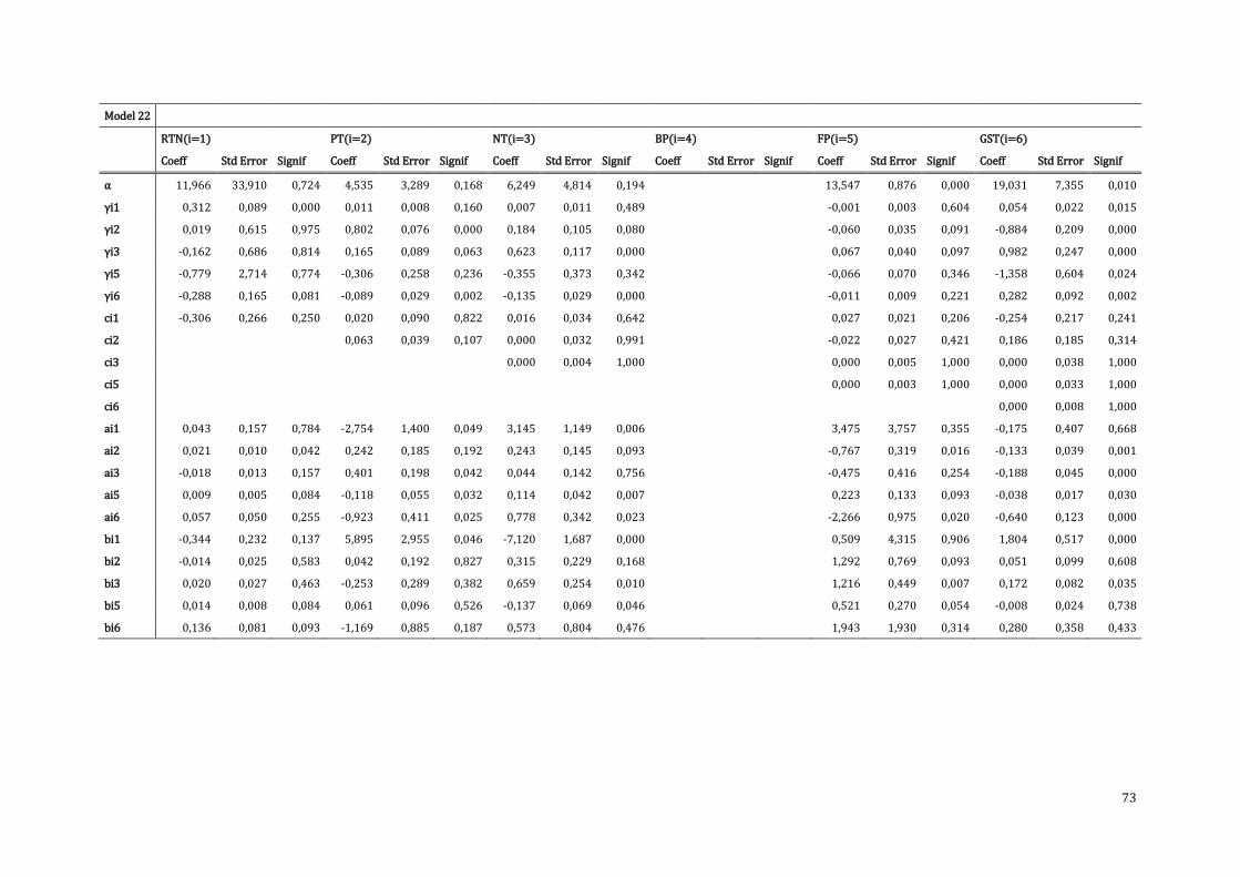
73

Model 22

RTN(i=1)

PT(i=2)

NT(i=3)

BP(i=4)

FP(i=5)

GST(i=6)

Coeff Std Error Signif Coeff Std Error Signif Coeff Std Error Signif Coeff Std Error Signif Coeff Std Error Signif Coeff Std Error Signif

α 11,966 33,910 0,724 4,535 3,289 0,168 6,249 4,814 0,194

13,547 0,876 0,000 19,031 7,355 0,010

γi1 0,312 0,089 0,000 0,011 0,008 0,160 0,007 0,011 0,489

-0,001 0,003 0,604 0,054 0,022 0,015

γi2 0,019 0,615 0,975 0,802 0,076 0,000 0,184 0,105 0,080

-0,060 0,035 0,091 -0,884 0,209 0,000

γi3 -0,162 0,686 0,814 0,165 0,089 0,063 0,623 0,117 0,000

0,067 0,040 0,097 0,982 0,247 0,000

γi5 -0,779 2,714 0,774 -0,306 0,258 0,236 -0,355 0,373 0,342

-0,066 0,070 0,346 -1,358 0,604 0,024

γi6 -0,288 0,165 0,081 -0,089 0,029 0,002 -0,135 0,029 0,000

-0,011 0,009 0,221 0,282 0,092 0,002

ci1 -0,306 0,266 0,250 0,020 0,090 0,822 0,016 0,034 0,642

0,027 0,021 0,206 -0,254 0,217 0,241

ci2

0,063 0,039 0,107 0,000 0,032 0,991

-0,022 0,027 0,421 0,186 0,185 0,314

ci3

0,000 0,004 1,000

0,000 0,005 1,000 0,000 0,038 1,000

ci5

0,000 0,003 1,000 0,000 0,033 1,000

ci6

0,000 0,008 1,000

ai1 0,043 0,157 0,784 -2,754 1,400 0,049 3,145 1,149 0,006

3,475 3,757 0,355 -0,175 0,407 0,668

ai2 0,021 0,010 0,042 0,242 0,185 0,192 0,243 0,145 0,093

-0,767 0,319 0,016 -0,133 0,039 0,001

ai3 -0,018 0,013 0,157 0,401 0,198 0,042 0,044 0,142 0,756

-0,475 0,416 0,254 -0,188 0,045 0,000

ai5 0,009 0,005 0,084 -0,118 0,055 0,032 0,114 0,042 0,007

0,223 0,133 0,093 -0,038 0,017 0,030

ai6 0,057 0,050 0,255 -0,923 0,411 0,025 0,778 0,342 0,023

-2,266 0,975 0,020 -0,640 0,123 0,000

bi1 -0,344 0,232 0,137 5,895 2,955 0,046 -7,120 1,687 0,000

0,509 4,315 0,906 1,804 0,517 0,000

bi2 -0,014 0,025 0,583 0,042 0,192 0,827 0,315 0,229 0,168

1,292 0,769 0,093 0,051 0,099 0,608

bi3 0,020 0,027 0,463 -0,253 0,289 0,382 0,659 0,254 0,010

1,216 0,449 0,007 0,172 0,082 0,035

bi5 0,014 0,008 0,084 0,061 0,096 0,526 -0,137 0,069 0,046

0,521 0,270 0,054 -0,008 0,024 0,738

bi6 0,136 0,081 0,093 -1,169 0,885 0,187 0,573 0,804 0,476

1,943 1,930 0,314 0,280 0,358 0,433

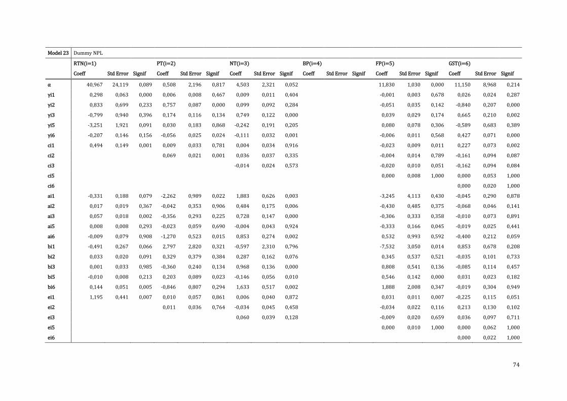
74

Model 23 Dummy NPL

RTN(i=1)

PT(i=2)

NT(i=3)

BP(i=4)

FP(i=5)

GST(i=6)

Coeff Std Error Signif Coeff Std Error Signif Coeff Std Error Signif Coeff Std Error Signif Coeff Std Error Signif Coeff Std Error Signif

α 40,967 24,119 0,089 0,508 2,196 0,817 4,503 2,321 0,052

11,830 1,030 0,000 11,150 8,968 0,214

γi1 0,298 0,063 0,000 0,006 0,008 0,467 0,009 0,011 0,404

-0,001 0,003 0,678 0,026 0,024 0,287

γi2 0,833 0,699 0,233 0,757 0,087 0,000 0,099 0,092 0,284

-0,051 0,035 0,142 -0,840 0,207 0,000

γi3 -0,799 0,940 0,396 0,174 0,116 0,134 0,749 0,122 0,000

0,039 0,029 0,174 0,665 0,210 0,002

γi5 -3,251 1,921 0,091 0,030 0,183 0,868 -0,242 0,191 0,205

0,080 0,078 0,306 -0,589 0,683 0,389

γi6 -0,207 0,146 0,156 -0,056 0,025 0,024 -0,111 0,032 0,001

-0,006 0,011 0,568 0,427 0,071 0,000

ci1 0,494 0,149 0,001 0,009 0,033 0,781 0,004 0,034 0,916

-0,023 0,009 0,011 0,227 0,073 0,002

ci2

0,069 0,021 0,001 0,036 0,037 0,335

-0,004 0,014 0,789 -0,161 0,094 0,087

ci3

-0,014 0,024 0,573

-0,020 0,010 0,051 -0,162 0,094 0,084

ci5

0,000 0,008 1,000 0,000 0,053 1,000

ci6

0,000 0,020 1,000

ai1 -0,331 0,188 0,079 -2,262 0,989 0,022 1,883 0,626 0,003

-3,245 4,113 0,430 -0,045 0,290 0,878

ai2 0,017 0,019 0,367 -0,042 0,353 0,906 0,484 0,175 0,006

-0,430 0,485 0,375 -0,068 0,046 0,141

ai3 0,057 0,018 0,002 -0,356 0,293 0,225 0,728 0,147 0,000

-0,306 0,333 0,358 -0,010 0,073 0,891

ai5 0,008 0,008 0,293 -0,023 0,059 0,690 -0,004 0,043 0,924

-0,333 0,166 0,045 -0,019 0,025 0,441

ai6 -0,009 0,079 0,908 -1,270 0,523 0,015 0,853 0,274 0,002

0,532 0,993 0,592 -0,400 0,212 0,059

bi1 -0,491 0,267 0,066 2,797 2,820 0,321 -0,597 2,310 0,796

-7,532 3,050 0,014 0,853 0,678 0,208

bi2 0,033 0,020 0,091 0,329 0,379 0,384 0,287 0,162 0,076

0,345 0,537 0,521 -0,035 0,101 0,733

bi3 0,001 0,033 0,985 -0,360 0,240 0,134 0,968 0,136 0,000

0,808 0,541 0,136 -0,085 0,114 0,457

bi5 -0,010 0,008 0,213 0,203 0,089 0,023 -0,146 0,056 0,010

0,546 0,142 0,000 0,031 0,023 0,182

bi6 0,144 0,051 0,005 -0,846 0,807 0,294 1,633 0,517 0,002

1,888 2,008 0,347 -0,019 0,304 0,949

ei1 1,195 0,441 0,007 0,010 0,057 0,861 0,006 0,040 0,872

0,031 0,011 0,007 -0,225 0,115 0,051

ei2

0,011 0,036 0,764 -0,034 0,045 0,458

-0,034 0,022 0,116 0,213 0,130 0,102

ei3

0,060 0,039 0,128

-0,009 0,020 0,659 0,036 0,097 0,711

ei5

0,000 0,010 1,000 0,000 0,062 1,000

ei6

0,000 0,022 1,000

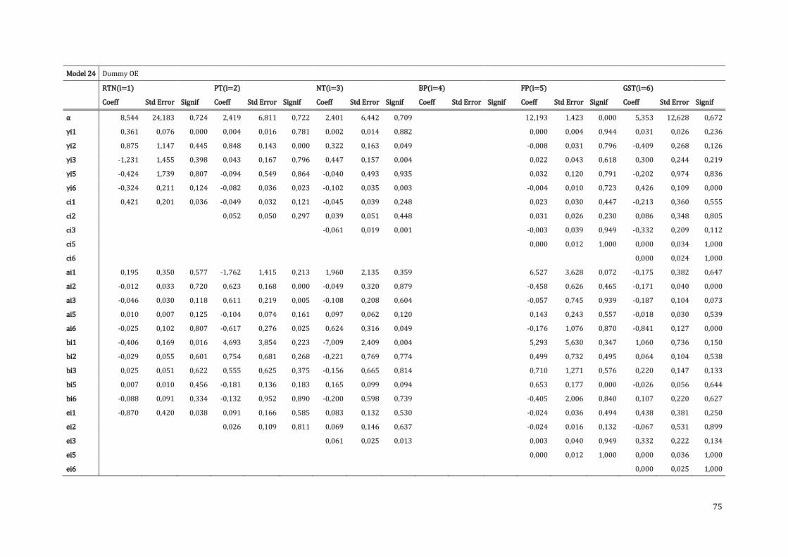
75

Model 24 Dummy OE

RTN(i=1)

PT(i=2)

NT(i=3)

BP(i=4)

FP(i=5)

GST(i=6)

Coeff Std Error Signif Coeff Std Error Signif Coeff Std Error Signif Coeff Std Error Signif Coeff Std Error Signif Coeff Std Error Signif

α 8,544 24,183 0,724 2,419 6,811 0,722 2,401 6,442 0,709

12,193 1,423 0,000 5,353 12,628 0,672

γi1 0,361 0,076 0,000 0,004 0,016 0,781 0,002 0,014 0,882

0,000 0,004 0,944 0,031 0,026 0,236

γi2 0,875 1,147 0,445 0,848 0,143 0,000 0,322 0,163 0,049

-0,008 0,031 0,796 -0,409 0,268 0,126

γi3 -1,231 1,455 0,398 0,043 0,167 0,796 0,447 0,157 0,004

0,022 0,043 0,618 0,300 0,244 0,219

γi5 -0,424 1,739 0,807 -0,094 0,549 0,864 -0,040 0,493 0,935

0,032 0,120 0,791 -0,202 0,974 0,836

γi6 -0,324 0,211 0,124 -0,082 0,036 0,023 -0,102 0,035 0,003

-0,004 0,010 0,723 0,426 0,109 0,000

ci1 0,421 0,201 0,036 -0,049 0,032 0,121 -0,045 0,039 0,248

0,023 0,030 0,447 -0,213 0,360 0,555

ci2

0,052 0,050 0,297 0,039 0,051 0,448

0,031 0,026 0,230 0,086 0,348 0,805

ci3

-0,061 0,019 0,001

-0,003 0,039 0,949 -0,332 0,209 0,112

ci5

0,000 0,012 1,000 0,000 0,034 1,000

ci6

0,000 0,024 1,000

ai1 0,195 0,350 0,577 -1,762 1,415 0,213 1,960 2,135 0,359

6,527 3,628 0,072 -0,175 0,382 0,647

ai2 -0,012 0,033 0,720 0,623 0,168 0,000 -0,049 0,320 0,879

-0,458 0,626 0,465 -0,171 0,040 0,000

ai3 -0,046 0,030 0,118 0,611 0,219 0,005 -0,108 0,208 0,604

-0,057 0,745 0,939 -0,187 0,104 0,073

ai5 0,010 0,007 0,125 -0,104 0,074 0,161 0,097 0,062 0,120

0,143 0,243 0,557 -0,018 0,030 0,539

ai6 -0,025 0,102 0,807 -0,617 0,276 0,025 0,624 0,316 0,049

-0,176 1,076 0,870 -0,841 0,127 0,000

bi1 -0,406 0,169 0,016 4,693 3,854 0,223 -7,009 2,409 0,004

5,293 5,630 0,347 1,060 0,736 0,150

bi2 -0,029 0,055 0,601 0,754 0,681 0,268 -0,221 0,769 0,774

0,499 0,732 0,495 0,064 0,104 0,538

bi3 0,025 0,051 0,622 0,555 0,625 0,375 -0,156 0,665 0,814

0,710 1,271 0,576 0,220 0,147 0,133

bi5 0,007 0,010 0,456 -0,181 0,136 0,183 0,165 0,099 0,094

0,653 0,177 0,000 -0,026 0,056 0,644

bi6 -0,088 0,091 0,334 -0,132 0,952 0,890 -0,200 0,598 0,739

-0,405 2,006 0,840 0,107 0,220 0,627

ei1 -0,870 0,420 0,038 0,091 0,166 0,585 0,083 0,132 0,530

-0,024 0,036 0,494 0,438 0,381 0,250

ei2

0,026 0,109 0,811 0,069 0,146 0,637

-0,024 0,016 0,132 -0,067 0,531 0,899

ei3

0,061 0,025 0,013

0,003 0,040 0,949 0,332 0,222 0,134

ei5

0,000 0,012 1,000 0,000 0,036 1,000

ei6

0,000 0,025 1,000

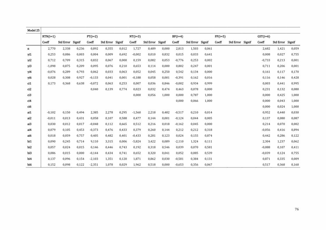
76

Model 25

RTN(i=1)

PT(i=2)

NT(i=3)

BP(i=4)

FP(i=5)

GST(i=6)

Coeff Std Error Signif Coeff Std Error Signif Coeff Std Error Signif Coeff Std Error Signif Coeff Std Error Signif Coeff Std Error Signif

α 2,770 2,338 0,236 0,892 0,355 0,012 1,727 0,489 0,000 2,813 1,503 0,061

2,682 1,421 0,059

γi1 0,253 0,086 0,003 0,004 0,009 0,692 -0,002 0,010 0,832 0,015 0,033 0,641

0,008 0,027 0,755

γi2 0,712 0,709 0,315 0,832 0,067 0,000 0,159 0,082 0,053 -0,776 0,253 0,002

-0,733 0,213 0,001

γi3 -1,098 0,875 0,209 0,095 0,076 0,210 0,653 0,114 0,000 0,802 0,247 0,001

0,711 0,206 0,001

γi4 -0,076 0,289 0,793 0,062 0,033 0,063 0,052 0,045 0,250 0,542 0,134 0,000

0,161 0,117 0,170

γi6 0,028 0,308 0,927 -0,133 0,041 0,001 -0,188 0,058 0,001 -0,391 0,162 0,016

0,116 0,146 0,428

ci1 0,173 0,368 0,638 -0,072 0,063 0,253 0,007 0,036 0,846 -0,002 0,934 0,999

0,003 0,441 0,995

ci2

0,040 0,139 0,774 0,023 0,032 0,474 0,463 0,078 0,000

0,231 0,132 0,080

ci3

0,000 0,056 1,000 0,000 0,787 1,000

0,000 0,425 1,000

ci4

0,000 0,066 1,000

0,000 0,043 1,000

ci6

0,000 0,024 1,000

ai1 -0,102 0,150 0,494 2,385 2,278 0,295 -1,560 2,218 0,482 -0,517 0,210 0,014

0,952 0,440 0,030

ai2 -0,011 0,013 0,431 0,058 0,107 0,588 0,477 0,144 0,001 -0,124 0,044 0,005

0,137 0,080 0,087

ai3 0,030 0,012 0,017 -0,048 0,112 0,665 0,512 0,216 0,018 -0,162 0,045 0,000

0,214 0,070 0,002

ai4 0,079 0,105 0,453 -0,373 0,476 0,433 0,379 0,260 0,144 0,212 0,212 0,318

-0,056 0,416 0,894

ai6 0,018 0,059 0,757 0,405 0,482 0,401 -0,433 0,281 0,123 0,024 0,155 0,874

0,442 0,286 0,122

bi1 0,090 0,245 0,714 9,110 3,315 0,006 -5,824 3,422 0,089 -2,110 1,324 0,111

2,304 1,237 0,062

bi2 0,057 0,024 0,015 0,146 0,446 0,743 0,192 0,318 0,546 0,039 0,070 0,581

-0,088 0,107 0,411

bi3 0,086 0,015 0,000 -0,144 0,434 0,741 0,652 0,320 0,041 0,052 0,085 0,539

-0,039 0,124 0,755

bi4 0,137 0,096 0,154 -2,103 1,351 0,120 1,871 0,862 0,030 -0,581 0,384 0,131

0,871 0,335 0,009

bi6 0,152 0,098 0,122 -2,351 1,078 0,029 1,962 0,518 0,000 -0,653 0,356 0,067

0,517 0,368 0,160

77

Model 26 Dummy NPL

RTN(i=1)

PT(i=2)

NT(i=3)

BP(i=4)

FP(i=5)

GST(i=6)

Coeff Std Error Signif Coeff Std Error Signif Coeff Std Error Signif Coeff Std Error Signif Coeff Std Error Signif Coeff Std Error Signif

α 4,333 1,709 0,011 1,012 0,213 0,000 1,640 0,271 0,000 2,398 0,612 0,000

1,787 0,599 0,003

γi1 0,400 0,085 0,000 0,007 0,008 0,337 0,017 0,012 0,158 0,020 0,042 0,626

0,015 0,032 0,632

γi2 0,092 0,477 0,847 0,867 0,037 0,000 0,247 0,036 0,000 -0,019 0,073 0,795

-0,030 0,027 0,262

γi3 -0,603 0,637 0,344 0,031 0,034 0,370 0,557 0,028 0,000 -0,007 0,113 0,948

-0,007 0,074 0,921

γi4 0,327 0,261 0,210 0,033 0,027 0,217 -0,008 0,038 0,831 0,324 0,103 0,002

-0,025 0,065 0,700

γi6 -0,349 0,276 0,205 -0,072 0,033 0,029 -0,087 0,054 0,106 -0,061 0,123 0,622

0,493 0,113 0,000

ci1 -0,134 0,247 0,588 0,000 0,037 0,996 -0,002 0,070 0,972 -0,179 0,374 0,632

-0,229 0,247 0,354

ci2

0,036 0,017 0,040 0,074 0,024 0,002 0,576 0,151 0,000

0,385 0,159 0,015

ci3

0,000 0,017 0,992 -0,002 0,180 0,992

0,000 0,153 0,998

ci4

-0,001 0,078 0,987

-0,002 0,130 0,987

ci6

0,000 0,155 0,998

ai1 0,263 0,094 0,005 3,466 0,899 0,000 -3,193 0,887 0,000 -0,263 0,206 0,200

0,812 0,399 0,042

ai2 0,035 0,011 0,001 -0,170 0,129 0,188 0,359 0,113 0,002 -0,084 0,032 0,008

0,081 0,047 0,087

ai3 0,028 0,013 0,032 -0,308 0,122 0,012 0,497 0,107 0,000 -0,131 0,041 0,002

0,182 0,051 0,000

ai4 -0,004 0,032 0,910 -1,519 0,435 0,000 1,390 0,391 0,000 -0,169 0,134 0,210

0,848 0,286 0,003

ai6 0,006 0,018 0,722 -0,384 0,277 0,165 0,331 0,284 0,243 -0,219 0,095 0,021

1,062 0,212 0,000

bi1 0,685 0,111 0,000 2,174 1,108 0,050 1,543 0,986 0,118 1,129 0,495 0,022

-2,176 0,473 0,000

bi2 -0,058 0,012 0,000 0,686 0,097 0,000 -0,229 0,082 0,005 0,043 0,082 0,604

-0,216 0,076 0,004

bi3 -0,067 0,017 0,000 -0,365 0,150 0,015 0,495 0,114 0,000 0,079 0,108 0,466

-0,335 0,099 0,001

bi4 -0,022 0,037 0,543 0,286 0,447 0,522 -1,180 0,416 0,005 0,398 0,238 0,095

-0,502 0,199 0,012

bi6 -0,050 0,029 0,083 0,347 0,250 0,166 -0,109 0,254 0,668 -0,221 0,150 0,140

0,119 0,154 0,439

ei1 0,295 0,443 0,504 -0,041 0,044 0,349 0,047 0,079 0,553 0,142 0,361 0,695

0,197 0,250 0,431

ei2

-0,032 0,057 0,574 -0,076 0,043 0,079 -0,576 0,147 0,000

-0,383 0,151 0,011

ei3

0,000 0,022 0,994 0,002 0,179 0,992

0,000 0,152 0,998

ei4

0,001 0,081 0,988

0,002 0,131 0,987

ei6

0,000 0,155 0,998

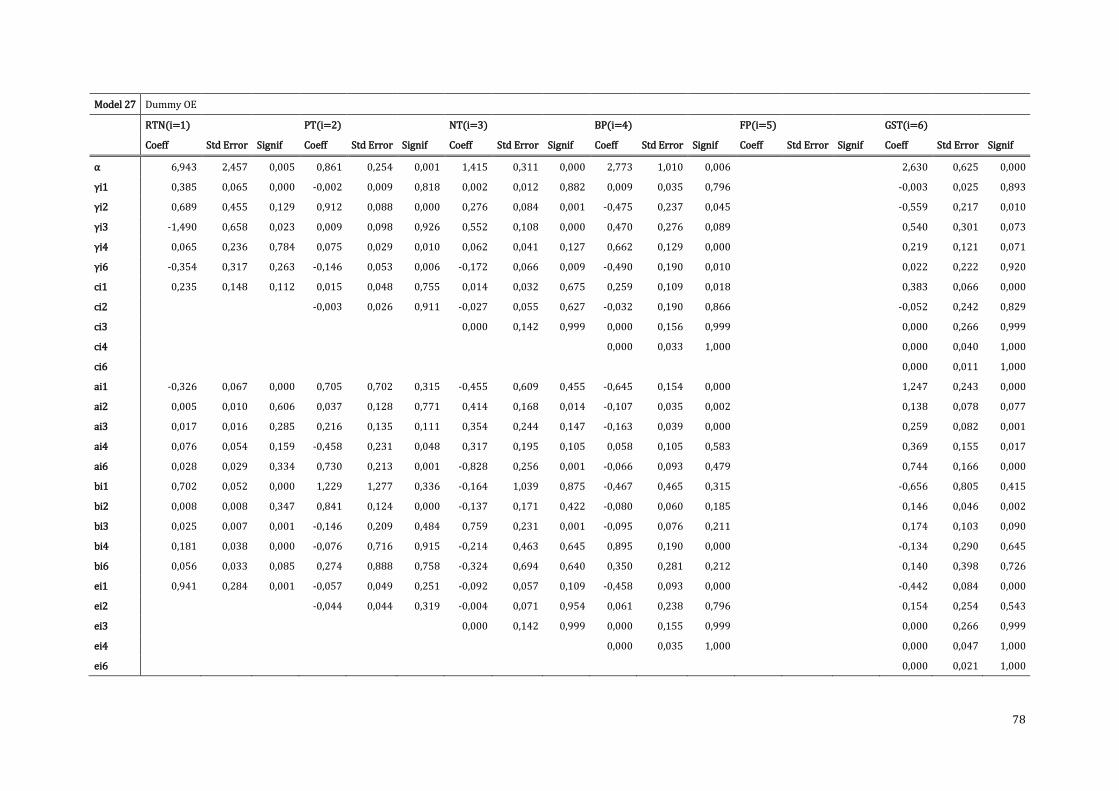
78

Model 27 Dummy OE

RTN(i=1)

PT(i=2)

NT(i=3)

BP(i=4)

FP(i=5)

GST(i=6)

Coeff Std Error Signif Coeff Std Error Signif Coeff Std Error Signif Coeff Std Error Signif Coeff Std Error Signif Coeff Std Error Signif

α 6,943 2,457 0,005 0,861 0,254 0,001 1,415 0,311 0,000 2,773 1,010 0,006

2,630 0,625 0,000

γi1 0,385 0,065 0,000 -0,002 0,009 0,818 0,002 0,012 0,882 0,009 0,035 0,796

-0,003 0,025 0,893

γi2 0,689 0,455 0,129 0,912 0,088 0,000 0,276 0,084 0,001 -0,475 0,237 0,045

-0,559 0,217 0,010

γi3 -1,490 0,658 0,023 0,009 0,098 0,926 0,552 0,108 0,000 0,470 0,276 0,089

0,540 0,301 0,073

γi4 0,065 0,236 0,784 0,075 0,029 0,010 0,062 0,041 0,127 0,662 0,129 0,000

0,219 0,121 0,071

γi6 -0,354 0,317 0,263 -0,146 0,053 0,006 -0,172 0,066 0,009 -0,490 0,190 0,010

0,022 0,222 0,920

ci1 0,235 0,148 0,112 0,015 0,048 0,755 0,014 0,032 0,675 0,259 0,109 0,018

0,383 0,066 0,000

ci2

-0,003 0,026 0,911 -0,027 0,055 0,627 -0,032 0,190 0,866

-0,052 0,242 0,829

ci3

0,000 0,142 0,999 0,000 0,156 0,999

0,000 0,266 0,999

ci4

0,000 0,033 1,000

0,000 0,040 1,000

ci6

0,000 0,011 1,000

ai1 -0,326 0,067 0,000 0,705 0,702 0,315 -0,455 0,609 0,455 -0,645 0,154 0,000

1,247 0,243 0,000

ai2 0,005 0,010 0,606 0,037 0,128 0,771 0,414 0,168 0,014 -0,107 0,035 0,002

0,138 0,078 0,077

ai3 0,017 0,016 0,285 0,216 0,135 0,111 0,354 0,244 0,147 -0,163 0,039 0,000

0,259 0,082 0,001

ai4 0,076 0,054 0,159 -0,458 0,231 0,048 0,317 0,195 0,105 0,058 0,105 0,583

0,369 0,155 0,017

ai6 0,028 0,029 0,334 0,730 0,213 0,001 -0,828 0,256 0,001 -0,066 0,093 0,479

0,744 0,166 0,000

bi1 0,702 0,052 0,000 1,229 1,277 0,336 -0,164 1,039 0,875 -0,467 0,465 0,315

-0,656 0,805 0,415

bi2 0,008 0,008 0,347 0,841 0,124 0,000 -0,137 0,171 0,422 -0,080 0,060 0,185

0,146 0,046 0,002

bi3 0,025 0,007 0,001 -0,146 0,209 0,484 0,759 0,231 0,001 -0,095 0,076 0,211

0,174 0,103 0,090

bi4 0,181 0,038 0,000 -0,076 0,716 0,915 -0,214 0,463 0,645 0,895 0,190 0,000

-0,134 0,290 0,645

bi6 0,056 0,033 0,085 0,274 0,888 0,758 -0,324 0,694 0,640 0,350 0,281 0,212

0,140 0,398 0,726

ei1 0,941 0,284 0,001 -0,057 0,049 0,251 -0,092 0,057 0,109 -0,458 0,093 0,000

-0,442 0,084 0,000

ei2

-0,044 0,044 0,319 -0,004 0,071 0,954 0,061 0,238 0,796

0,154 0,254 0,543

ei3

0,000 0,142 0,999 0,000 0,155 0,999

0,000 0,266 0,999

ei4

0,000 0,035 1,000

0,000 0,047 1,000

ei6

0,000 0,021 1,000

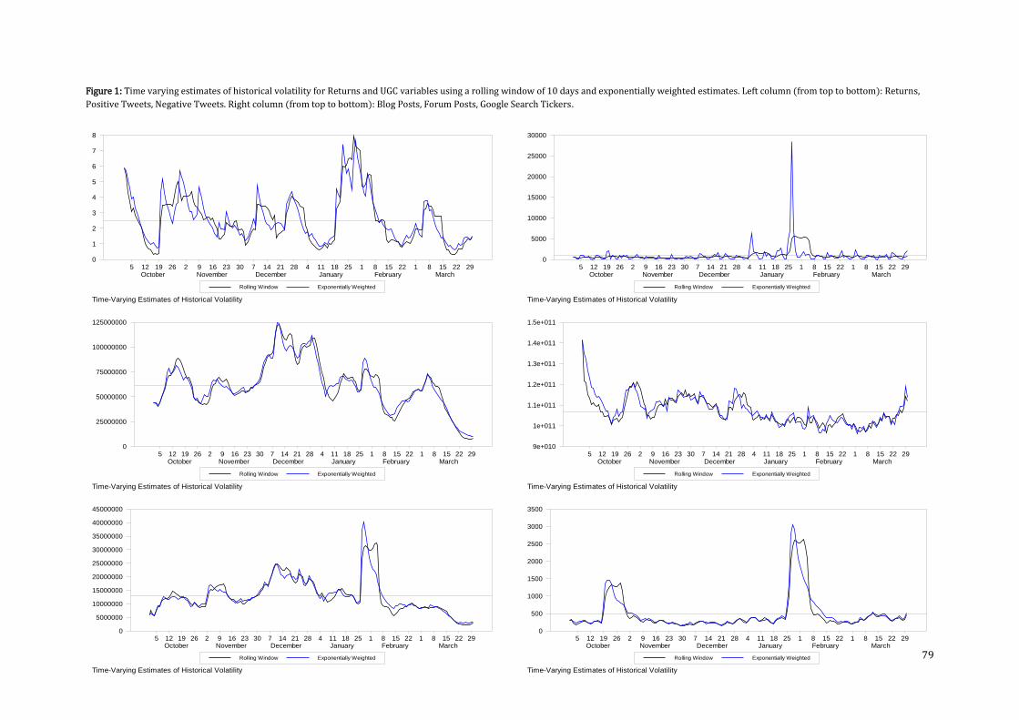
79

Figure 1: Time varying estimates of historical volatility for Returns and UGC variables using a rolling window of 10 days and exponentially weighted estimates. Left column (from top to bottom): Returns,

Positive Tweets, Negative Tweets. Right column (from top to bottom): Blog Posts, Forum Posts, Google Search Tickers.

Time-Varying Estimates of Historical Volatility

Rolling Window Exponentially Weighted

5 12 19 26 2 9 16 23 30 7 14 21 28 4 11 18 25 1 8 15 22 1 8 15 22 29October November December January February March

0

1

2

3

4

5

6

7

8

Time-Varying Estimates of Historical Volatility

Rolling Window Exponentially Weighted

5 12 19 26 2 9 16 23 30 7 14 21 28 4 11 18 25 1 8 15 22 1 8 15 22 29October November December January February March

0

25000000

50000000

75000000

100000000

125000000

Time-Varying Estimates of Historical Volatility

Rolling Window Exponentially Weighted

5 12 19 26 2 9 16 23 30 7 14 21 28 4 11 18 25 1 8 15 22 1 8 15 22 29October November December January February March

0

5000000

10000000

15000000

20000000

25000000

30000000

35000000

40000000

45000000

Time-Varying Estimates of Historical Volatility

Rolling Window Exponentially Weighted

5 12 19 26 2 9 16 23 30 7 14 21 28 4 11 18 25 1 8 15 22 1 8 15 22 29October November December January February March

0

5000

10000

15000

20000

25000

30000

Time-Varying Estimates of Historical Volatility

Rolling Window Exponentially Weighted

5 12 19 26 2 9 16 23 30 7 14 21 28 4 11 18 25 1 8 15 22 1 8 15 22 29October November December January February March

9e+010

1e+011

1.1e+011

1.2e+011

1.3e+011

1.4e+011

1.5e+011

Time-Varying Estimates of Historical Volatility

Rolling Window Exponentially Weighted

5 12 19 26 2 9 16 23 30 7 14 21 28 4 11 18 25 1 8 15 22 1 8 15 22 29October November December January February March

0

500

1000

1500

2000

2500

3000

3500