Volatility Spillovers Between Oil Prices And Stock Returns ...

HAL Id: hal-02314397https://hal.archives-ouvertes.fr/hal-02314397

Submitted on 12 Oct 2019

HAL is a multi-disciplinary open accessarchive for the deposit and dissemination of sci-entific research documents, whether they are pub-lished or not. The documents may come fromteaching and research institutions in France orabroad, or from public or private research centers.

L’archive ouverte pluridisciplinaire HAL, estdestinée au dépôt et à la diffusion de documentsscientifiques de niveau recherche, publiés ou non,émanant des établissements d’enseignement et derecherche français ou étrangers, des laboratoirespublics ou privés.

Volatility Spillovers Between Oil Prices And StockReturns: A Focus On Frontier Markets

Mathieu Gomes, Anissa Chaibi

To cite this version:Mathieu Gomes, Anissa Chaibi. Volatility Spillovers Between Oil Prices And Stock Returns: A FocusOn Frontier Markets. Journal of Applied Business Research, Clute Institute, 2014, 30. �hal-02314397�

https://hal.archives-ouvertes.fr/hal-02314397

https://hal.archives-ouvertes.fr

The Journal of Applied Business Research – March/April 2014 Volume 30, Number 2

Copyright by author(s); CC-BY 509 The Clute Institute

Volatility Spillovers Between Oil Prices

And Stock Returns: A Focus

On Frontier Markets Mathieu Gomes, Université d’Auvergne Clermont, France

Anissa Chaibi, IPAG Business School, France

ABSTRACT

Frontier markets are increasingly sought by investors in search of higher returns and low

correlation with traditional assets. As such, it is important for financial market participants to

understand the volatility transmission mechanism across these markets in order to make better

portfolio allocation decisions. This paper employs a bivariate BEKK-GARCH(1,1) model to

simultaneously estimate the mean and conditional variance between equity stock markets (twenty-

one national frontier stock indices and two broad indices – the MSCI Frontier Markets and the

MSCI World) and oil prices. We examine weekly returns from February 8, 2008 to February 1,

2013 and find significant transmission of shocks and volatility between oil prices and some of the

examined markets. Moreover, this spillover effect is sometimes bidirectional.

Keywords: Volatility Spillovers; Oil Prices; Stock Returns; Multivariate GARCH; Diversification; Frontier

Markets

1. INTRODUCTION

rude oil is probably the physical commodity that most affects the state of the economy. This impact can

take place through various paths. When crude oil prices rise, cost of production of goods and services

increases, and so do transportation and heating costs. This, in turn, can lead to inflationary pressures and

thus restricted consumption from consumers. This produces a negative effect to capital markets, consumer

confidence, and the macroeconomy as a whole. There are thus, various theoretical reasons for which oil prices can

have a significant impact on financial markets, and stock markets in particular. One of them is that the value of stock

prices in equity asset valuation models theoretically equals the sum of future discounted earnings expectation of

companies or future cash flows. Therefore, changes in crude oil prices can directly have an impact on stock prices

through the expected cash flows on the one hand, and through the discount rate on the other hand.

The first and most intuitive way through which oil prices can affect stock prices is by the channel of

expected cash flows. Oil is a crucial input in the production of goods and services, and therefore, a rise in oil prices

is likely to increase production costs, which in turn will reduce margins, cash flows and thus stock prices. But oil

prices can also affect stock valuations through the rate that is used to discount future cash flows. Indeed, rising oil

prices can create inflationary pressures that will ultimately lead to the decision-making by central banks to tighten

their monetary policies and raise interest rates. This can have tremendous implications for companies as corporate

investment decisions can be affected directly by changes in the discount rate. Moreover, a change in interest rates

will impact company financing through higher borrowing costs and a lower market value relative to book value,

which will further damage a company’s ability to raise new funds.

However, it is worth noting that not all companies will react the same way to changes in crude oil prices.

Indeed, the direction of stock price reactions will depend on whether the company is an oil producer or an oil

consumer. Oil producers will profit from an oil price increase while oil consumers will suffer from it. Overall, since

the great majority of companies are oil consumers, it is logical to expect a negative effect of oil prices on stock

prices.

C



To the better of our knowledge, no previous study has examined the effect of oil price shocks on frontier

markets. Our paper aims to fill this gap by making use of a rich database and innovative econometric techniques.

Section 2 discusses findings of previous works on interactions between oil prices and stock markets with a specific

focus on emerging markets. Section 3 introduces the concept of frontier markets. A preliminary analysis of our

database is provided in Section 4. Section 5 introduces our empirical methodology. Results are discussed in Section

6, while Section 7 concludes and gives some policy implications.

2. LITERATURE REVIEW

A number of research papers have explicitly examined the relationship between oil markets and economic

variables, such as GDP growth rates, inflation, employment, and exchange rates (Hamilton, 1983; Gisser &

Goodwin, 1986; Mork, 1989; Hooker, 1996; among others). The impact of oil price changes on the world economy

is indeed large. According to Adelman (1993), ‘‘Oil is so significant in the international economy that forecasts of

economic growth are routinely qualified with the caveat: ‘Provided there is no oil shock.’’’ As another proof of that

importance, the International Monetary Fund (2000) estimated that a US$5 per barrel price increase had tremendous

effects on the state of the economy with a reduction of global economic growth by 0.3% in the following year.

Surprisingly, while understanding the relationship between oil price changes and stock markets may appear

crucial to energy policy planning, energy risk management and portfolio diversification, these links have only been

examined recently. Jones and Kaul (1996) were the first to test the reaction of international stock markets (Canada,

UK, Japan, and USA) to oil price shocks, based on the standard cash-flow dividend valuation model. They find that

for Canada and the US, this reaction can be entirely accounted for by the impact of the oil shocks on cash flows.

Huang et al. (1996), using an unrestricted Vector Autoregressive (VAR) model, show a significant link between the

stock returns of certain American oil companies and oil price changes. However, there is no evidence of a link

between oil prices and market indices such as the S&P 500. In contrast, Sadorsky (1999), using a Vector

Autoregressive (VAR) framework, shows that oil prices play an important role in affecting economic activity. His

results also suggest an asymmetric relationship, as changes in economic activity don’t seem to have an impact on oil

prices.

Ciner (2001), using non-linear causality tests, provides empirical evidence that oil shocks significantly

affect stock index returns in the US in a non-linear manner, and that the returns also have impacts on crude oil

futures. Park and Ratti (2008) show that oil price shocks have a statistically significant impact on real stock returns

contemporaneously and/or within the following month in the U.S. and 13 European countries over the period

running from January 1986 to December 2005 and that Norway, as an oil exporter, shows a statistically significantly

positive response of real stock returns to an oil price increase.

More recently, some studies have examined the extent of oil price impacts on stock prices from a sector-by-

sector perspective. For example, El-Sharif et al. (2005) show that the stock returns of UK Oil & Gas companies are

positively correlated to oil price increases. Boyer and Filion (2007) obtain similar results for Oil & Gas returns in

Canada. Arouri and Nguyen (2010), using various econometric techniques, suggest that the sensitivity of European

sector stock returns to oil price changes greatly differ from one sector to another, with Oil & Gas stocks profiting

from oil price increases. Similarly, Arouri, Bellalah, and Nguyen (2011) show that, on the basis of short-term

analysis, strong positive links are found in some GCC (Gulf Cooperation Council) countries between oil prices and

stock markets, and that this causality generally runs from oil prices to stock markets.

Despite various studies focusing on price spillovers between oil and stock markets, it is only recently that

some attention has been paid to possible volatility spillovers between these two markets. Using a multivariate

GARCH model, Malik and Hammoudeh (2005) find significant volatility transmission between second moments of

the US equity and global oil markets. In that same study, they find that the three examined Gulf equity markets

(Bahrain, Kuwait, and Saudi Arabia) receive volatility from the oil market, with Saudi Arabia featuring an

interesting characteristic, i.e. a significant volatility spillover from the Saudi equity market to the global oil market,

underlining the major role played by Saudi Arabia in the global oil market. Agren (2006), using an asymmetric

BEKK model, finds strong evidence of volatility spillovers (albeit relatively small) from oil prices to stock markets

in Japan, Norway, the UK, and the US. Malik and Ewing (2009) study volatility spillovers between oil prices and



five US equity sector indices (Financials, Industrials, Consumer Services, Health Care, and Technology) and

conclude in favor of significant transmission of shocks and volatility between oil prices and some of the examined

market sectors.

Using a recent generalized VAR-GARCH approach to examine the extent of volatility transmission

between oil and stock markets in Europe and the US at the sector level, Arouri, Jouini, and Nguyen (2011) find

evidence of significant volatility spillover. Their study suggests that the transmission is usually unidirectional from

oil markets to stock markets in Europe, but bidirectional in the US. Chang et al. (2012), using various econometric

models, investigate the conditional correlations and volatility spillovers between the crude oil and financial markets,

and find little evidence of volatility transmission between the oil market and major stock indices (FTSE100, Dow

Jones, and S&P500). These results would tend to confirm that volatility transmission between oil and stock markets

only occurs in some sectors.

3. A FOCUS ON “FRONTIER MARKETS”

To the best of my knowledge, no research has so far been done about possible volatility transmission

between oil markets and frontier markets (apart from GCC countries). The term “frontier markets” was coined by

the International Finance Corporation (IFC), a private sector arm of the World Bank Group, in 1992 to reflect a

subset of emerging market economies. Frontier markets are investable but have lower market capitalization (usually

under 17% of GDP) and liquidity than the more developed "traditional" emerging markets, which makes them

inherently riskier investments but also provides potential opportunities for investors to take advantage of

privatizations and increased listings on local exchanges over time. As a result, they may also provide better returns.

Investments in these markets are thus generally pursued by investors who are seeking higher returns, and who are

willing to assume the higher level of risk associated with such markets. Among these risks are political instability,

poor liquidity, inadequate regulation, substandard financial reporting, and large currency fluctuations. Apart from

risks, investing in frontier markets is a smart diversification to an equity portfolio, as these markets have

comparatively less correlation to developed markets, and in good times, can likely beat the returns of other markets.

Despite the growing attention to frontier markets among the investment community, very little research

actually includes them. However, the contributions to this particular topic reach similar conclusions: frontier

markets may offer promising diversification benefits due to low correlations with developed equity markets

(Speidell & Krohne, 2007; Jayasuriya & Shambora 2009; Berger, Pukthuanthong, & Yang, 2011).

No official list of frontier markets countries has so far been established, but the number usually ranges

between twenty-five and thirty countries. Oil economies often have the largest representation in frontier market

indices. For example, five Gulf Cooperation Council (GCC) countries (Qatar, UAE, Oman, Bahrain, and Kuwait)

currently make up about 60% of the MSCI Frontier Markets Index. Frontier markets are widely diverse in terms of

income, geography and degree of economic development. For example, the GCC countries are among the richest

economies globally on a per capita basis, while many of the key Sub-Saharan economies are among the poorest (the

average GDP per capita of GCC economies is approximately $43,300 PPP while the average GDP per capita of the

frontier Africa and Asia countries is under $2,000 PPP). But the middle class is growing in many frontier markets as

improvements in logistics, better access to technology, the spread of mobile phones and better use of natural

resources have begun to raise millions out of poverty while boosting consumption trends.

4. DATA SET

Equity market data are obtained from MSCI. In this paper, we use a set of data consisting of twenty-one

national aggregate stock market indices (Argentina, Bahrain, Bulgaria, Jordan, Kazakhstan, Kenya, Kuwait,

Lebanon, Mauritius, Nigeria, Oman, Pakistan, Qatar, Romania, Saudi Arabia, Slovenia, Sri Lanka, Tunisia, United

Arab Emirates, Ukraine, and Viet-Nam) and two broader stock indices (MSCI Frontier Markets and MSCI World),

together with a measure of the world oil price (Brent). All data are at the weekly frequency and cover a five-year

period ranging from February 8, 2008 to February 1, 2013, yielding a total of 261 observations. We use weekly data

because as suggested by Arouri and Nguyen (2010), they appear to be less noisy than daily data, while still capturing

much of the information content of stock indices and oil prices.



Table 1: Summary Statistics for Weekly Percentage Returns on Twenty-One National Stock Market Indices,

Two Broad Stock Indices and the Oil Price

ARG BAH BRENT BUL FM

Mean -0.000392 -0.006716 0.002214 -0.005666 -0.002289

Median 0.002725 -0.003219 0.005534 -0.002640 0.000000

Maximum 0.190511 0.083382 0.273051 0.193988 0.072381

Minimum -0.264352 -0.191904 -0.223806 -0.340314 -0.141460

Std. Dev. 0.061570 0.031999 0.051031 0.050725 0.025259

Skewness -0.648030 -1.713767 -0.238456 -1.161328 -1.694278

Kurtosis 6.587412 11.23679 7.276525 11.67068 10.88979

Jarque-Bera 158.2236 865.5709 201.3627 876.2579 801.8263

Probability 0.000000 0.000000 0.000000 0.000000 0.000000

Observations 261 261 261 261 261

JOR KAZ KEN KUW LEB MAU NIG

Mean -0.002876 -0.000785 0.001149 -0.002344 -0.000651 -0.000475 -0.001280

Median -0.001944 -0.000461 0.002064 -0.000693 -0.002999 -0.002000 -0.000537

Maximum 0.096996 0.339806 0.237935 0.182310 0.160940 0.117474 0.199916

Minimum -0.129781 -0.275896 -0.144212 -0.192224 -0.109269 -0.200252 -0.180769

Std. Dev. 0.028759 0.055016 0.037551 0.037484 0.030326 0.034643 0.047633

Skewness -0.588160 0.345285 0.660617 -0.519418 1.157897 -0.561908 -0.006575

Kurtosis 6.526772 10.74318 9.986814 9.539805 10.11749 8.666132 6.297023

Jarque-Bera 150.3126 657.2164 549.8534 476.8495 609.2340 362.8772 118.2170

Probability 0.000000 0.000000 0.000000 0.000000 0.000000 0.000000 0.000000

Observations 261 261 261 261 261 261 261

OMA PAK QAT ROM SAU SLO SRI

Mean -0.001893 -0.001231 0.000503 -0.000461 -0.000288 -0.003351 0.002483

Median 0.000857 0.002903 0.000849 0.007082 0.001653 -0.000979 -0.001682

Maximum 0.118208 0.166830 0.137242 0.222458 0.144495 0.120431 0.421636

Minimum -0.199966 -0.238645 -0.203556 -0.293018 -0.166560 -0.197436 -0.131955

Std. Dev. 0.033284 0.044879 0.037994 0.058200 0.038431 0.037662 0.045690

Skewness -1.395272 -1.124315 -0.930632 -0.819155 -0.376414 -0.979714 3.529371

Kurtosis 11.32211 9.013421 9.588668 6.868070 6.752524 7.744587 31.31229

Jarque-Bera 837.8604 448.2410 509.7639 191.9005 159.2990 286.5613 9259.100

Probability 0.000000 0.000000 0.000000 0.000000 0.000000 0.000000 0.000000

Observations 261 261 261 261 261 261 261

TUN UAE UKR VIE WORLD

Mean 0.000867 -0.001789 -0.006956 -0.001192 0.000362

Median 0.000509 -0.001154 -0.007190 -0.000214 0.002840

Maximum 0.090079 0.230320 0.251340 0.163965 0.123224

Minimum -0.129134 -0.278740 -0.204843 -0.175901 -0.200515

Std. Dev. 0.026764 0.050793 0.056337 0.050716 0.032802

Skewness -0.522514 -1.007268 0.197675 0.032316 -0.915448

Kurtosis 7.223866 9.837133 5.131759 4.284099 8.946894

Jarque-Bera 205.8977 552.5015 51.12010 17.97734 421.0553

Probability 0.000000 0.000000 0.000000 0.000125 0.000000

Observations 261 261 261 261 261

We can see from Table 1 that out of twenty-one national aggregate equity indices, seventeen display

negative average weekly returns, which is not surprising given the characteristics of the covered period and the

impact of the economic and financial crisis since 2008. The broader MSCI Frontier Markets index displays a

negative average weekly return of -0.2289% while the MSCI World index exhibits a positive average weekly return

of 0.0362%, largely driven by a recent bull market in the United States which represent the largest constituent of the

index. The Brent posted an average weekly return of 0.2214% over the period.

At the country level, the highest weekly mean return is posted by the Sri Lanka stock market with a weekly

average of 0.25% while the lowest average weekly return comes from Ukraine (-0.70%). The highest weekly return

was posted by Sri Lanka on the week ranging from May 18, 2009 to May 22, 2009 (+42%), followed by Kazakhstan

(+34% on the week ranging from October 27, 2008 to October 31, 2008).



The lowest return comes from Bulgaria (-34%) on the week ranging from October 6, 2008 to October 10,

2008, followed by neighboring Romania (-29% on the week ranging from January 5, 2009 to January 9, 2009). The

Brent gained up to 27% (from December 29, 2008 to January 2, 2009) while its biggest weekly drop was -22%

(from December 1, 2008 to December 5, 2008). Over the whole period, the best performer was Sri Lanka with a

49% gain while the worst performer was the Ukrainian stock market, which lost approximately 90% of its value.

Weekly standard deviations range from 2.67% (Tunisia) to 6.16% (Argentina). The MSCI Frontier Markets

index varied 2.53% while the MSCI World index and the Brent experienced volatilities of 3.28% and 5.10%

respectively.

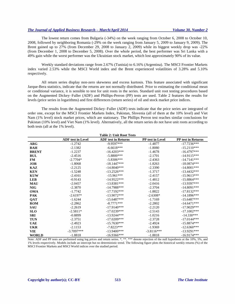
All return series display non-zero skewness and excess kurtosis. This feature associated with significant

Jarque-Bera statistics, indicate that the returns are not normally distributed. Prior to estimating the conditional mean

or conditional variance, it is sensible to test for unit roots in the series. Standard unit root testing procedures based

on the Augmented Dickey–Fuller (ADF) and Phillips-Perron (PP) tests are used. Table 2 features the results for

levels (price series in logarithms) and first differences (return series) of oil and stock market price indices.

The results from the Augmented Dickey–Fuller (ADF) tests indicate that the price series are integrated of

order one, except for the MSCI Frontier Markets Index, Pakistan, Slovenia (all of them at the 10% level) and Viet

Nam (1% level) stock market prices, which are stationary. The Phillips Perron test reaches similar conclusions for

Pakistan (10% level) and Viet Nam (1% level). Alternatively, all the return series do not have unit roots according to

both tests (all at the 1% level).

Table 2: Unit Root Tests

ADF test in Level ADF test in Returns PP test in Level PP test in Returns

ARG -1.2742 -9.9597*** -1.4877 -17.7236***

BAH -2.1382 -6.6618*** -1.8080 -15.2110***

BRENT -1.2237 -16.4203*** -1.4678 -16.4797***

BUL -2.4516 -5.8800*** -2.1701 -14.9115***

FM -2.7704* -5.8306*** -2.4363 -14.7141***

JOR -1.8068 -18.1447*** -1.8263 -18.0874***

KAZ -2.2125 -14.8040*** -2.3390 -14.8001***

KEN -1.5248 -13.2526*** -1.3717 -13.4432***

KUW -2.4161 -15.961*** -2.4157 -15.9613***

LEB -0.9143 -14.9522*** -1.4812 -15.8864***

MAU -2.0457 -13.8381*** -2.0416 -13.9397***

NIG -2.3870 -14.7988*** -2.3704 -14.8091***

OMA -1.7742 -17.7192*** -1.8822 -17.8132***

PAK -2.6197* -13.9072*** -2.6308* -14.1896***

QAT -1.6244 -15.6487*** -1.7169 -15.6487***

ROM -2.2862 -8.7771*** -2.2802 -14.6471***

SAU -2.2619 -17.9140*** -2.2120 -17.9029***

SLO -2.5811* -17.0239*** -2.5143 -17.1002***

SRI -0.8899 -13.9244*** -1.0216 -14.330***

TUN -2.3751 -17.0209*** -2.3728 -17.0144***

UAE -2.4923 -15.7630*** -2.4924 -15.8874***

UKR -2.1153 -7.8223*** -1.9369 -12.6360***

VIE -3.7097*** -13.9400*** -3.8116*** -13.9291***

WORLD -1.8818 -16.9366*** -1.8818 -16.9174***

Note: ADF and PP tests are performed using log prices and return series. *, **, *** denote rejection of the null hypothesis at the 10%, 5%, and

1% levels respectively. Models include an intercept but no deterministic trend. The following figure plots the historical weekly returns (%) of the

MSCI Frontier Markets and MSCI World indices over the studied period.



Figure 1: Weekly Returns of Broad Stock Market Indices (MSCI Frontier Markets and MSCI World)

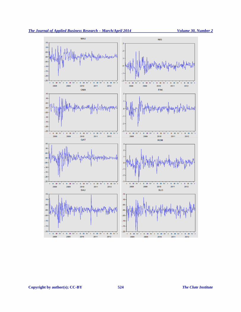
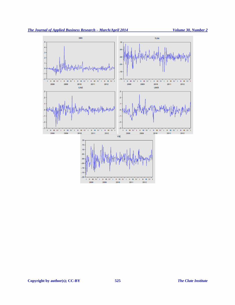
Plots of each national equity market returns are enclosed in the appendix.

The following figure plots the historical weekly returns (%) of crude oil (Brent) over the studied period.

Figure 2: Weekly Changes in the Oil Price (Brent)

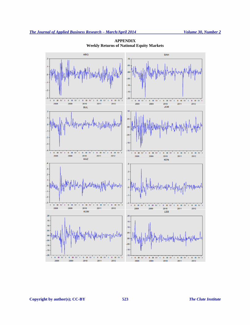
We can see that all markets experienced increased volatility during 2008 due to the financial crisis. Overall,

frontier markets appear to be very volatile with countries such as Argentina, Romania, and Ukraine featuring mean

annualized standard deviations above 40.0%. However, the MSCI Frontier Markets index displays a mean weekly

volatility of 2.53%, which is actually lower than the MSCI World’s (3.28%). This tends to suggest that despite high

individual volatilities, correlation between frontier equity markets is low.

Table 3 shows the correlation matrix for all considered markets. It tends to confirm the above statement, as

correlations between frontier markets are indeed very low with an average value of 28.0%. The average correlation

coefficient between frontier markets and the Brent is 27.6% while average correlation between frontier markets and

the MSCI World index amounts to 37.4%. All these figures would tend to confirm the diversifying power of frontier

markets stocks within a portfolio.

Correlations with oil are positive, suggesting that during the studied period, frontier stock markets moved

together with oil prices. The highest correlation is between the MSCI World index and the oil market (0.5279). This

result is expected because of the large proportion of American stocks within the index. The lowest significant

correlation with oil market is obtained for Tunisia (0.1313).



Table 3: Correlation Matrix of Return Series (P-Values in Parentheses) ARG BAH BRENT BUL FM JOR KAZ KEN KUW LEB MAU NIG OMA PAK QAT ROM SAU SLO SRI TUN UAE UKR VIE WORLD

ARG

1.0000

--------

-

BAH 0.0955

(0.124)

1.0000

---------

BRENT 0.4347

(0.000)

0.1243

(0.045)

1.0000

---------

BUL 0.4679

(0.000)

0.2473

(0.000)

0.3510

(0.000)

1.0000

---------

FM 0.4115

(0.000)

0.4137

(0.000)

0.3979

(0.000)

0.4843

(0.000)

1.0000

---------

JOR 0.1724

(0.005)

0.2942

(0.000)

0.0689

(0.267)

0.3446

(0.000)

0.4710

(0.000)

1.0000

---------

KAZ 0.5229

(0.000)

0.0927

(0.135)

0.4805

(0.000)

0.3893

(0.000)

0.3399

(0.000)

0.1630

(0.008)

1.0000

--------

KEN 0.2789

(0.000)

0.2260

(0.000)

0.1908

(0.002)

0.3140

(0.000)

0.3368

(0.000)

0.2931

(0.000)

0.2652

(0.000)

1.0000

---------

KUW 0.1969

(0.001)

0.3138

(0.000)

0.1601

(0.010)

0.1964

(0.001)

0.8057

(0.000)

0.2771

(0.000)

0.1041

(0.093)

0.1583

(0.010)

1.0000

--------

LEB 0.3598

(0.000)

0.2351

(0.000)

0.2618

(0.000)

0.2337

(0.000)

0.3462

(0.000)

0.2122

(0.001)

0.2362

(0.000)

0.2023

(0.001)

0.1612

(0.009)

1.0000

--------

MAU 0.2878

(0.000)

0.1912

(0.002)

0.3293

(0.000)

0.5230

(0.000)

0.4254

(0.000)

0.2800

(0.000)

0.2958

(0.000)

0.3307

(0.000)

0.1542

(0.013)

0.2046

(0.001)

1.0000

---------

NIG 0.0237

(0.703)

0.1204

(0.052)

0.1184

(0.156)

0.1136

(0.067)

0.2873

(0.000)

0.1065

(0.086)

0.0845

(0.174)

0.0817

(0.188)

-0.0102

(0.870)

0.1228

(0.048)

0.0614

(0.323)

1.0000

---------

OMA 0.2449

(0.000)

0.2584

(0.000)

0.3500

(0.000)

0.3389

(0.000)

0.6493

(0.000)

0.3331

(0.000)

0.1446

(0.020)

0.3613

(0.000)

0.4333

(0.000)

0.1411

(0.023)

0.2645

(0.000)

0.1043

(0.093)

1.0000

---------

PAK 0.1092

(0.078)

0.1042

(0.093)

0.0699

(0.261)

0.0595

(0.338)

0.3412

(0.000)

-0.0397

(0.523)

0.0867

(0.163)

0.0727

(0.242)

0.3256

(0.000)

0.0469

(0.451)

0.1557

(0.012)

0.0723

(0.244)

0.2457

(0.000)

1.0000

---------

QAT 0.2592

(0.000)

0.2707

(0.000)

0.2395

(0.000)

0.3639

(0.000)

0.7420

(0.000)

0.4510

(0.000)

0.1714

(0.010)

0.2942

(0.000)

0.5109

(0.000)

0.2906

(0.000)

0.3237

(0.000)

0.0876

(0.158)

0.5896

(0.000)

0.1181

(0.057)

1.0000

---------

ROM 0.4735

(0.000)

0.2418

(0.000)

0.3788

(0.000)

0.5544

(0.000)

0.5709

(0.000)

0.2066

(0.001)

0.4789

(0.000)

0.3027

(0.000)

0.3312

(0.000)

0.2670

(0.000)

0.4684

(0.000)

0.2543

(0.000)

0.3059

(0.000)

0.1646

(0.008)

0.3638

(0.000)

1.0000

---------

SAU 0.2664

(0.000)

0.2402

(0.000)

0.1512

(0.015)

0.3921

(0.000)

0.6058

(0.000)

0.5031

(0.000)

0.0895

(0.149)

0.2687

(0.000)

0.3608

(0.000)

0.1999

(0.001)

0.3259

(0.000)

0.1440

(0.020)

0.5179

(0.000)

0.1696

(0.000)

0.6210

(0.000)

0.2662

(0.000)

1.0000

---------

SLO 0.5751

(0.000)

0.1366

(0.027)

0.4708

(0.000)

0.5838

(0.000)

0.5052

(0.000)

0.3389

(0.000)

0.4543

(0.000)

0.2856

(0.000)

0.2174

(0.000)

0.2893

(0.000)

0.5061

(0.000)

0.1272

(0.040)

0.3022

(0.000)

0.0996

(0.108)

0.3074

(0.000)

0.5753

(0.000)

0.3824

(0.000)

1.0000

---------

SRI 0.2073

(0.001)

0.1191

(0.055)

0.2418

(0.000)

0.2168

(0.000)

0.2686

(0.000)

0.1639

(0.008)

0.2487

(0.000)

0.2307

(0.000)

0.0884

(0.154)

0.0995

(0.109)

0.3208

(0.000)

0.1149

(0.064)

0.2181

(0.000)

0.0364

(0.559)

0.1351

(0.029)

0.2327

(0.000)

0.1830

(0.003)

0.3060

(0.000)

1.0000

---------

TUN 0.1853

(0.003)

0.0962

(0.121)

0.1313

(0.034)

0.2344

(0.000)

0.2442

(0.000)

0.1375

(0.026)

0.1292

(0.037)

0.2188

(0.000)

0.1490

(0.016)

0.0771

(0.214)

0.1793

(0.004)

0.0833

(0.180)

0.2043

(0.001)

0.0837

(0.178)

0.0771

(0.214)

0.2321

(0.000)

0.2208

(0.000)

0.2316

(0.000)

0.1279

(0.039)

1.0000

---------

UAE 0.1950

(0.002)

0.3519

(0.000)

0.3156

(0.000)

0.3552

(0.000)

0.7654

(0.000)

0.4470

(0.000)

0.1912

(0.002)

0.2188

(0.000)

0.4763

(0.000)

0.2278

(0.000)

0.3670

(0.000)

0.1025

(0.099)

0.6552

(0.000)

0.2635

(0.000)

0.6333

(0.000)

0.3095

(0.000)

0.5874

(0.000)

0.3453

(0.000)

0.1921

(0.002)

0.1859

(0.003)

1.0000

---------

UKR 0.4063

(0.000)

0.1783

(0.004)

0.3340

(0.000)

0.4078

(0.000)

0.4157

(0.000)

0.2380

(0.000)

0.4850

(0.000)

0.2680

(0.000)

0.1776

(0.004)

0.2789

(0.000)

0.3191

(0.000)

0.1478

(0.017)

0.2779

(0.000)

0.1683

(0.006)

0.2798

(0.000)

0.4644

(0.000)

0.2829

(0.000)

0.3997

(0.000)

0.2706

(0.000)

0.1013

(0.103)

0.2787

(0.000)

1.0000

---------

VIE 0.2326

(0.000)

0.0916

(0.140)

0.2869

(0.000)

0.3321

(0.000)

0.3448

(0.000)

0.1906

(0.002)

0.2083

(0.001)

0.1556

(0.012)

0.1347

(0.030)

0.1418

(0.022)

0.3418

(0.000)

0.0803

(0.196)

0.2552

(0.000)

0.0017

(0.978)

0.3238

(0.000)

0.2975

(0.000)

0.2735

(0.000)

0.3664

(0.000)

0.1141

(0.066)

0.1275

(0.040)

0.2798

(0.000)

0.2780

(0.000)

1.0000

---------

WORLD 0.6636

(0.000)

0.0614

(0.323)

0.5279

(0.000)

0.5801

(0.000)

0.4898

(0.000)

0.1730

(0.005)

0.6027

(0.000)

0.2757

(0.000)

0.2542

(0.000)

0.3244

(0.000)

0.3860

(0.000)

0.0912

(0.142)

0.2506

(0.000)

0.1239

(0.046)

0.3186

(0.000)

0.6474

(0.000)

0.2695

(0.000)

0.6534

(0.000)

0.1561

(0.012)

0.2580

(0.000)

0.2791

(0.000)

0.4382

(0.000)

0.3204

(0.000)

1.0000

---------



Before moving to the analysis of potential spillovers, it is interesting to examine short-term relationships

between oil price changes and stock market returns. To do this, I perform a Granger causality test (for a lag equal to

one) to examine the causal linkages between these series. Table 4 reports the results obtained.

Table 4: Results of the Granger Causality Tests (P-Values)

Oil to Stocks Stocks to Oil

ARG 0.3174 0.8402

BAH 0.0151 0.1053

BUL 0.0126 0.1137

FM 0.0304 0.0711

JOR 0.0000 0.6258

KAZ 0.3884 0.7722

KEN 0.0065 0.4141

KUW 0.2452 0.1182

LEB 0.0065 0.2575

MAU 0.1574 0.1948

NIG 0.0324 0.3140

OMA 0.0001 0.7754

PAK 0.2880 0.6814

QAT 0.0092 0.0563

ROM 0.7098 0.2733

SAU 0.0000 0.3402

SLO 0.1322 0.6833

SRI 0.1778 0.1173

TUN 0.7459 0.5896

UAE 0.0037 0.0631

UKR 0.0009 0.1338

VIE 0.0585 0.3438

WORLD 0.9683 0.4878

The results show that, in the short-run oil price shocks Granger-cause changes in stock market returns in,

Jordan, Kenya, Lebanon, Oman, Qatar, Saudi Arabia, the UAE, and Ukraine (1%) and to some extent in Bahrain,

Bulgaria, the Frontier Markets index, Nigeria (5%), and Viet Nam (10%). There is also evidence of causality from

the Frontier Markets Index, Qatar and the UAE stock markets to oil prices.

5. METHODOLOGY

The GARCH-type approach has received a special interest from almost all previous studies dealing with

volatility modeling and forecasting of commodities prices. When the aim is to investigate volatility interdependence

and transmission mechanisms among different time-series, multivariate settings such as the CCC-MGARCH model

of Bollerslev (1990), the BEKK-GARCH model of Baba et al. (1990), or the DCC-MGARCH model of Engle

(2002) are more relevant than univariate models. Empirical results reported in Hassan and Malik (2007) and

Agnolucci (2009), among others, confirm the superiority of these models and show that they are able to

satisfactorily capture the stylized facts of the commodity-price conditional volatility and the dynamics of volatility

interaction.

The first step in the bivariate GARCH methodology is to specify the mean equation. Accordingly, the mean

equations for oil and stock return series are given by:

(1)

(2)

where and are the returns between time t-1 and t on oil and stock series respectively, and are lagged

returns on oil and stock series, and are long term drift coefficients, and and are error terms. Various

models were tested to specify the mean equation (ARMA type) but the coefficients were not statistically significant

so I ended up using the classical first order autoregressive model.



In this paper, we use a bivariate GARCH (Generalized Auto Regressive Conditionally Heteroscedastic)

model to estimate the conditional variance of oil and stock index returns. In addition, I employ the BEKK (named

after Baba, Engle, Kraft, and Kroner, 1990) parameterization of the multivariate GARCH model, which does not

impose the restriction of constant correlation among variables over time. The model addresses the difficulty with

VECH of ensuring that the H matrix is always positive definite by incorporating quadratic forms.

The BEKK parameterization for the bivariate GARCH(1,1) model is represented by:

(3)

where the individual elements for C, A and B matrices are given as:

A =

B =

C =

where is the conditional variance matrix, C is an upper triangular matrix of parameters, B is a 2 x 2 matrix of

parameters which depicts the extent to which current levels of conditional variances are related to past conditional

variances, and A is a 2 x 2 matrix of parameters that measures the extent to which conditional variances are

correlated with past squared errors. In other words, A captures the effect of shocks or events on volatility. The

positive definiteness of the covariance matrix is ensured owing to the quadratic nature of the terms on the equation’s

right hand side.

Expanding the conditional variance for each equation in the bivariate BEKK-GARCH(1,1) model gives:

As can be seen, the conditional variance of the stock market (respectively oil market) depends not only on

its own past variances and innovations, but also on those of the oil market (respectively stock market). This feature

permits the direct transmission of volatility and shocks from one market to another. Overall, this model allows me to

capture both return and volatility spillover effects between stock and oil markets.

Under the assumption of conditional normality, the parameters of a multivariate GARCH model can be

estimated by maximizing the log-likelihood function:

where θ denotes all the unknown parameters to be estimated, N is the number of series and T is the number of

observations.

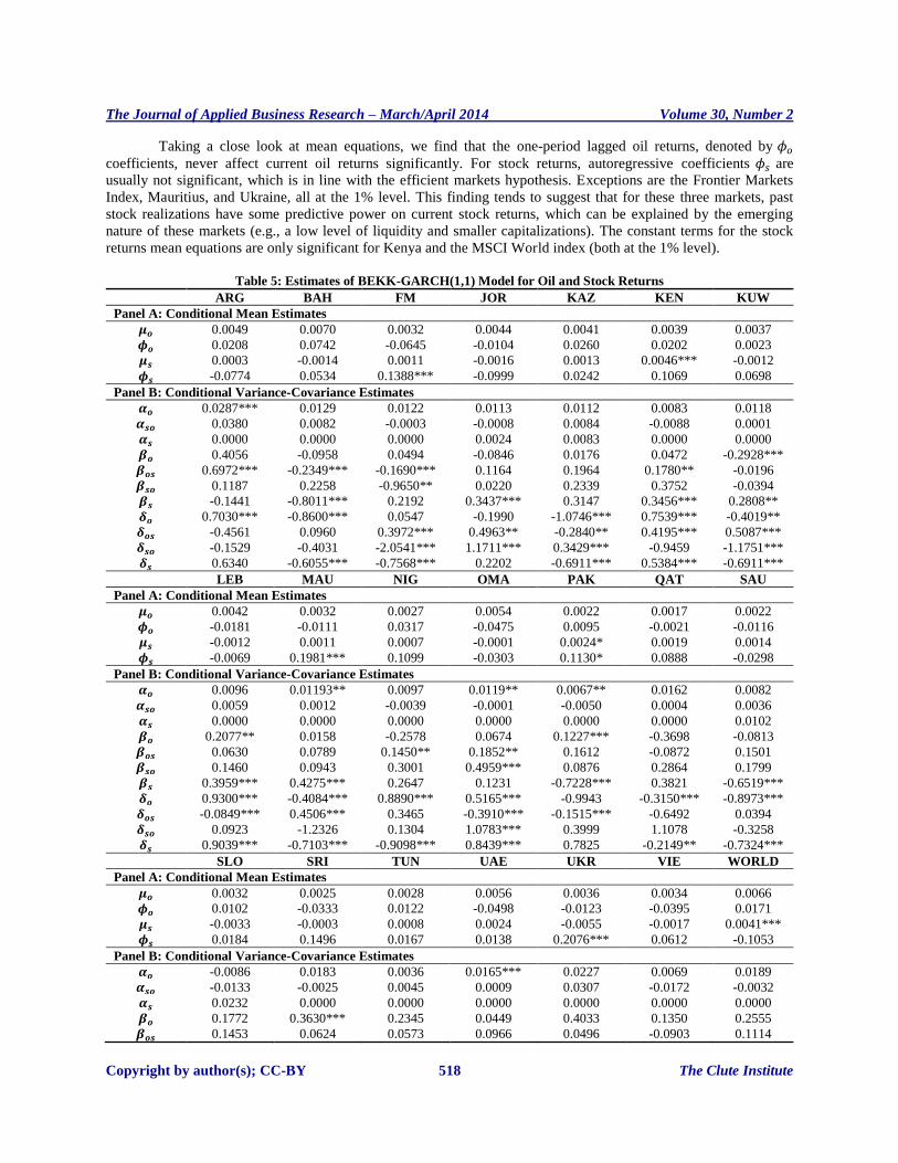
6. EMPIRICAL RESULTS

In this section, we present in Table 5 the empirical results from estimating the bivariate BEKK-

GARCH(1,1) model for all pairs of oil and stock market returns and we discuss the extent of volatility transmission.

There are no reported data for Bulgaria and Romania as the model was unable to converge for these two markets.

The symbols *, ** and *** indicate significance at 10%, 5%, and 1% levels respectively.



Taking a close look at mean equations, we find that the one-period lagged oil returns, denoted by

coefficients, never affect current oil returns significantly. For stock returns, autoregressive coefficients are

usually not significant, which is in line with the efficient markets hypothesis. Exceptions are the Frontier Markets

Index, Mauritius, and Ukraine, all at the 1% level. This finding tends to suggest that for these three markets, past

stock realizations have some predictive power on current stock returns, which can be explained by the emerging

nature of these markets (e.g., a low level of liquidity and smaller capitalizations). The constant terms for the stock

returns mean equations are only significant for Kenya and the MSCI World index (both at the 1% level).

Table 5: Estimates of BEKK-GARCH(1,1) Model for Oil and Stock Returns

ARG BAH FM JOR KAZ KEN KUW

Panel A: Conditional Mean Estimates

0.0049 0.0070 0.0032 0.0044 0.0041 0.0039 0.0037

0.0208 0.0742 -0.0645 -0.0104 0.0260 0.0202 0.0023

0.0003 -0.0014 0.0011 -0.0016 0.0013 0.0046*** -0.0012

-0.0774 0.0534 0.1388*** -0.0999 0.0242 0.1069 0.0698

Panel B: Conditional Variance-Covariance Estimates

0.0287*** 0.0129 0.0122 0.0113 0.0112 0.0083 0.0118

0.0380 0.0082 -0.0003 -0.0008 0.0084 -0.0088 0.0001

0.0000 0.0000 0.0000 0.0024 0.0083 0.0000 0.0000

0.4056 -0.0958 0.0494 -0.0846 0.0176 0.0472 -0.2928***

0.6972*** -0.2349*** -0.1690*** 0.1164 0.1964 0.1780** -0.0196

0.1187 0.2258 -0.9650** 0.0220 0.2339 0.3752 -0.0394

-0.1441 -0.8011*** 0.2192 0.3437*** 0.3147 0.3456*** 0.2808**

0.7030*** -0.8600*** 0.0547 -0.1990 -1.0746*** 0.7539*** -0.4019**

-0.4561 0.0960 0.3972*** 0.4963** -0.2840** 0.4195*** 0.5087***

-0.1529 -0.4031 -2.0541*** 1.1711*** 0.3429*** -0.9459 -1.1751***

0.6340 -0.6055*** -0.7568*** 0.2202 -0.6911*** 0.5384*** -0.6911***

LEB MAU NIG OMA PAK QAT SAU


0.0042 0.0032 0.0027 0.0054 0.0022 0.0017 0.0022

-0.0181 -0.0111 0.0317 -0.0475 0.0095 -0.0021 -0.0116

-0.0012 0.0011 0.0007 -0.0001 0.0024* 0.0019 0.0014

-0.0069 0.1981*** 0.1099 -0.0303 0.1130* 0.0888 -0.0298


0.0096 0.01193** 0.0097 0.0119** 0.0067** 0.0162 0.0082

0.0059 0.0012 -0.0039 -0.0001 -0.0050 0.0004 0.0036

0.0000 0.0000 0.0000 0.0000 0.0000 0.0000 0.0102

0.2077** 0.0158 -0.2578 0.0674 0.1227*** -0.3698 -0.0813

0.0630 0.0789 0.1450** 0.1852** 0.1612 -0.0872 0.1501

0.1460 0.0943 0.3001 0.4959*** 0.0876 0.2864 0.1799

0.3959*** 0.4275*** 0.2647 0.1231 -0.7228*** 0.3821 -0.6519***

0.9300*** -0.4084*** 0.8890*** 0.5165*** -0.9943 -0.3150*** -0.8973***

-0.0849*** 0.4506*** 0.3465 -0.3910*** -0.1515*** -0.6492 0.0394

0.0923 -1.2326 0.1304 1.0783*** 0.3999 1.1078 -0.3258

0.9039*** -0.7103*** -0.9098*** 0.8439*** 0.7825 -0.2149** -0.7324***

SLO SRI TUN UAE UKR VIE WORLD


0.0032 0.0025 0.0028 0.0056 0.0036 0.0034 0.0066

0.0102 -0.0333 0.0122 -0.0498 -0.0123 -0.0395 0.0171

-0.0033 -0.0003 0.0008 0.0024 -0.0055 -0.0017 0.0041***

0.0184 0.1496 0.0167 0.0138 0.2076*** 0.0612 -0.1053


-0.0086 0.0183 0.0036 0.0165*** 0.0227 0.0069 0.0189

-0.0133 -0.0025 0.0045 0.0009 0.0307 -0.0172 -0.0032

0.0232 0.0000 0.0000 0.0000 0.0000 0.0000 0.0000

0.1772 0.3630*** 0.2345 0.0449 0.4033 0.1350 0.2555

0.1453 0.0624 0.0573 0.0966 0.0496 -0.0903 0.1114



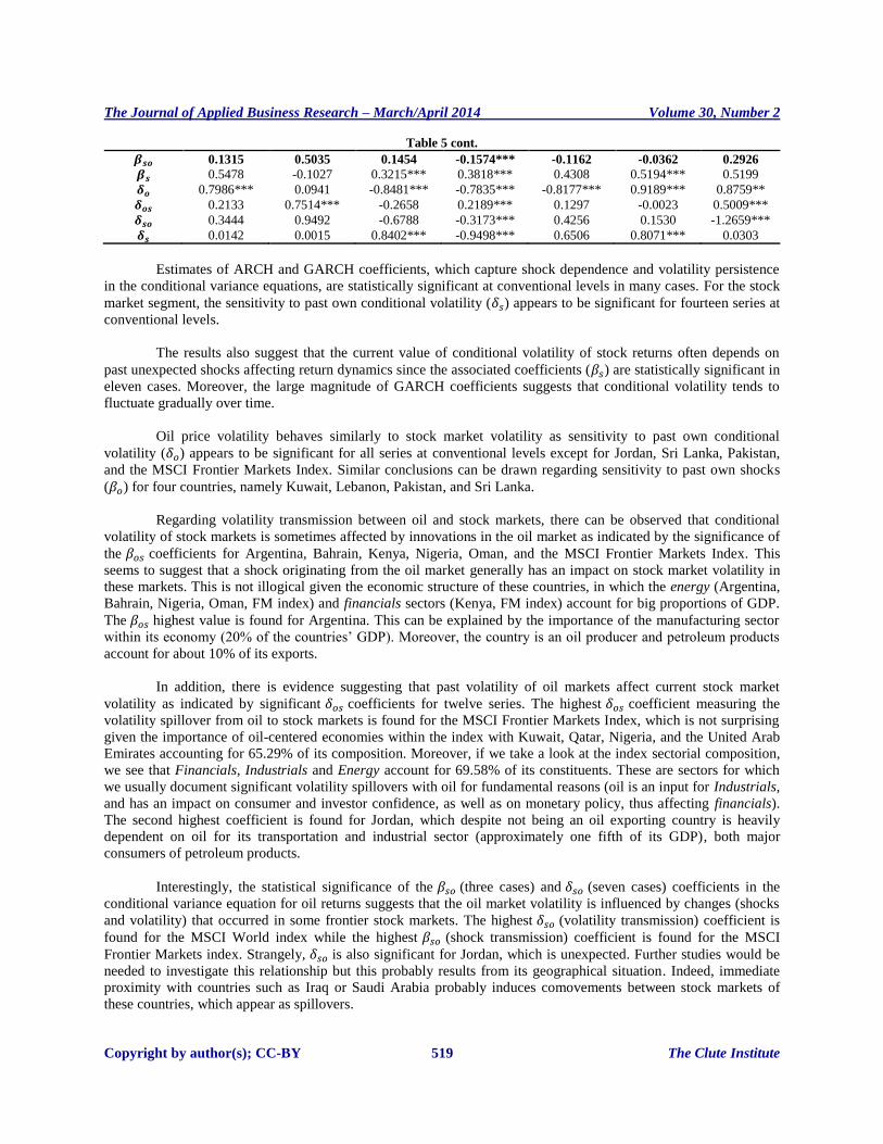
Table 5 cont.

0.1315 0.5035 0.1454 -0.1574*** -0.1162 -0.0362 0.2926

0.5478 -0.1027 0.3215*** 0.3818*** 0.4308 0.5194*** 0.5199

0.7986*** 0.0941 -0.8481*** -0.7835*** -0.8177*** 0.9189*** 0.8759**

0.2133 0.7514*** -0.2658 0.2189*** 0.1297 -0.0023 0.5009***

0.3444 0.9492 -0.6788 -0.3173*** 0.4256 0.1530 -1.2659***

0.0142 0.0015 0.8402*** -0.9498*** 0.6506 0.8071*** 0.0303

Estimates of ARCH and GARCH coefficients, which capture shock dependence and volatility persistence

in the conditional variance equations, are statistically significant at conventional levels in many cases. For the stock

market segment, the sensitivity to past own conditional volatility ( ) appears to be significant for fourteen series at

conventional levels.

The results also suggest that the current value of conditional volatility of stock returns often depends on

past unexpected shocks affecting return dynamics since the associated coefficients ( ) are statistically significant in

eleven cases. Moreover, the large magnitude of GARCH coefficients suggests that conditional volatility tends to

fluctuate gradually over time.

Oil price volatility behaves similarly to stock market volatility as sensitivity to past own conditional

volatility ( ) appears to be significant for all series at conventional levels except for Jordan, Sri Lanka, Pakistan,

and the MSCI Frontier Markets Index. Similar conclusions can be drawn regarding sensitivity to past own shocks

( ) for four countries, namely Kuwait, Lebanon, Pakistan, and Sri Lanka.

Regarding volatility transmission between oil and stock markets, there can be observed that conditional

volatility of stock markets is sometimes affected by innovations in the oil market as indicated by the significance of

the coefficients for Argentina, Bahrain, Kenya, Nigeria, Oman, and the MSCI Frontier Markets Index. This

seems to suggest that a shock originating from the oil market generally has an impact on stock market volatility in

these markets. This is not illogical given the economic structure of these countries, in which the energy (Argentina,

Bahrain, Nigeria, Oman, FM index) and financials sectors (Kenya, FM index) account for big proportions of GDP.

The highest value is found for Argentina. This can be explained by the importance of the manufacturing sector

within its economy (20% of the countries’ GDP). Moreover, the country is an oil producer and petroleum products

account for about 10% of its exports.

In addition, there is evidence suggesting that past volatility of oil markets affect current stock market

volatility as indicated by significant coefficients for twelve series. The highest coefficient measuring the

volatility spillover from oil to stock markets is found for the MSCI Frontier Markets Index, which is not surprising

given the importance of oil-centered economies within the index with Kuwait, Qatar, Nigeria, and the United Arab

Emirates accounting for 65.29% of its composition. Moreover, if we take a look at the index sectorial composition,

we see that Financials, Industrials and Energy account for 69.58% of its constituents. These are sectors for which

we usually document significant volatility spillovers with oil for fundamental reasons (oil is an input for Industrials,

and has an impact on consumer and investor confidence, as well as on monetary policy, thus affecting financials).

The second highest coefficient is found for Jordan, which despite not being an oil exporting country is heavily

dependent on oil for its transportation and industrial sector (approximately one fifth of its GDP), both major

consumers of petroleum products.

Interestingly, the statistical significance of the (three cases) and (seven cases) coefficients in the

conditional variance equation for oil returns suggests that the oil market volatility is influenced by changes (shocks

and volatility) that occurred in some frontier stock markets. The highest (volatility transmission) coefficient is

found for the MSCI World index while the highest (shock transmission) coefficient is found for the MSCI

Frontier Markets index. Strangely, is also significant for Jordan, which is unexpected. Further studies would be

needed to investigate this relationship but this probably results from its geographical situation. Indeed, immediate

proximity with countries such as Iraq or Saudi Arabia probably induces comovements between stock markets of

these countries, which appear as spillovers.



These findings are interesting as they suggest wide bi-directional transmission of both shock and volatility

between oil and some frontier stock markets, but also between oil and the MSCI World Index, which is not illogical.

Indeed, Arouri et al. (2011) demonstrated that the United States, which represents the major part (53.9%) of the

MSCI World Index composition, feature this bidirectional relationship between oil and stock markets. Moreover, the

volatility spillover effect is often strong (usually significant at the 1% level). Regarding the direction of

transmission, and coefficients with statistical significance are more numerous than their and

counterparts, suggesting that spillovers from oil to stock markets are more usual than spillovers going from stocks to

the oil market, which is in line with the majority of previous studies.

Summarizing all, direct volatility transmission between oil and stock returns is significantly present for

many of the studied markets, including the MSCI World Index. Regarding the transmission’s direction, shock and

volatility spillovers happen more often running from oil to stock markets than from stock markets to the oil market,

but there are divergences between countries, which is something to be expected given the heterogeneity of frontier

market economies.

Finally, it is important to note that the set of data analyzed in this paper pertains to a very turbulent period

in financial markets and that consequently, systematic factors may have played a role and biased the spillover results

to some extent as spillovers usually increase during crisis periods under the effects of important financial instability

and economic uncertainties.

7. CONCLUSION

This paper examined the transmission of shocks and volatility between oil prices and Frontier stock

markets. The statistical model includes a parameterization of the conditional variance-covariance of oil price

changes and stock returns, specifically the bivariate BEKK-GARCH(1,1) model, which enables the analysis of

spillovers in both returns and conditional variance. Aggregate stock market data representing twenty-three frontier

markets, as well as two broad equity indices (MSCI World and MSCI Frontier Markets) are used. My analysis uses

weekly data from February 8, 2008 to February 1, 2013, and provides estimates of the extent to which shocks and

volatility are transmitted between oil returns and the returns of Frontier equity markets (+ the MSCI World Index).

My results suggest significant volatility interaction between oil and some frontier stock markets. Moreover, the

spillover effect appears to be bidirectional in many markets, which is a characteristic that differs from what has been

found for developed stock markets where the transmission is usually unidirectional (from oil to stock markets).

However, empirical results show that the spillovers run more often from oil to stock markets.

The findings of the study offer several avenues for future research. First, the link between oil and frontier

stock markets should eventually be examined over an extended period of time. Second, further evidence drawn from

a deeper decomposition of spillovers (spillover, interdependence, comovements and independence) should be

produced to examine the robustness of the findings. These would require more elaborate models (MCMS). Finally,

hedging effectiveness could be analyzed for these markets in order to compute optimal weights and hedge ratios for

oil-stock portfolio holdings. Overall, this study is of particular interest for portfolio management since it offers

insight into markets that still provide valuable opportunities for portfolio diversification. In all, this paper improves

our knowledge of how stock markets relate to oil prices.

AUTHOR INFORMATION

Mathieu Gomes is a commodity index structuring analyst at BNP Paribas. He holds a Master’s degree in financial

markets and a Master's degree in management from the Université d’Auvergne, Clermont-Ferrand, France. His

research interests include commodities, investment strategies, and financial economics. E-mail:

[email protected]

Dr. Anissa Chaibi is a researcher at IPAG Business School, France. Her research areas are development economics,

finance, and econometrics. Her most recent articles are published in refereed journals such as Economic Modelling,

Energy Policy and Journal of Applied Business Research. E-mail: [email protected] (Corresponding author)

mailto:[email protected]

mailto:[email protected]



REFERENCES

1. Adelman, M. A. (1993). The economics of petroleum supply: Papers 1962–1993. Massachusetts Institute of

Technology.

2. Agnolucci, P. (2009). Volatility In crude oil futures: A comparison of the predictive ability of GARCH and

implied volatility models. Energy Economics, 31, 316-321.

3. Agren, M. (2006). Does oil price uncertainty transmit to stock markets? (Working Paper 2006, p. 23).

Department of Economics/Uppsala University.

4. Arouri, M., & Nguyen, D. K. (2010). Oil prices, stock markets and portfolio investment: Evidence from

sector analysis in europe over the last decade. Energy Policy, 38, 4528-4539.

5. Arouri, M., Bellalah, M., & Nguyen, D. K. (2011). Further evidence on the response of stock prices in

GCC countries to oil price shocks. International Journal of Business, 16.

6. Arouri, M., Jouini, J., & Nguyen, D. K. (2011). Volatility spillovers between oil prices and stock sector

returns: Implications for portfolio management. Journal of International Money and Finance, 30, 1387-

1405.

7. Arouri, M., Jouini, J., & Nguyen, D. K. (2012). On the impact of oil price fluctuations on european equity

markets: Volatility spillover and hedging effectiveness. Energy Economics, 34, §11-617.

8. Baba, Y., Engle, R.F., Kraft, D., & Kroner, K. (1990). Multivariate simultaneous generalized ARCH.

(Unpublished Manuscript). University of California, San Diego.

9. Berger, D., Pukthuanthong, K., & Yang, J. J. (2011). International diversification with frontier markets.

Journal of Financial Economics, 101, 227-242.

10. Boyer, M. M., & Filion, D. (2007). Common and fundamental factors in stock returns of Canadian oil and

gas companies. Energy Economics, 29, 428-453.

11. Chang, C., McAleer, M., & Tansuchat, R. (2012). Conditional correlations and volatility spillovers between

crude oil and stock index returns. North American Journal of Economics and Finance.

12. Ciner, C. (2001). Energy shocks and financial markets: Nonlinear linkages. Studies in Non-Linear

Dynamics and Econometrics, 5, 203-212.

13. El-Sharif, I., Brown, D., Burton, B., Nixon, B., & Russel, A. (2005). Evidence on the nature and extent of

the relationship between oil and equity value in UK. Energy Economics, 27, 819-830.

14. Engle, R. F., & Kroner, K. F. (1995). Multivariate simultaneous generalized ARCH. Econometric Theory,

11, 122-150.

15. Engle, R. F. (2002). Dynamic conditional correlation: A simple class of multivariate GARCH models.

Journal of Business and Economic Statistics, 20, 339-350.

16. Gisser, M., & Goodwin, T. H. (1986). Crude oil and the macroeconomy: Tests of some popular notions:

Note. Journal of Money, Credit and Banking, 18(1), 95-103.

17. Hamilton, J. D. (1983). Oil and the macroeconomy since World War II. Journal of Political Economy,

91(2), 228-248.

18. Hassan, H., & Malik, F. (2007). Multivariate GARCH model of sector volatility transmission. Quarterly

Review of Economics and Finance, 47, 470-480.

19. Hooker, M. A. (1996). What happened to the oil price-macroeconomy relationship? Journal of Monetary

Economics, 38, 195-213.

20. Huang, R. D., Masulis R. W., & Stoll, H. R. (1996). Energy shocks and financial markets. Journal of

Futures Markets, 16, 1-27.

21. Jayasuriya, S., & Shambora, W. (2009). Oops, we should have diversified! Applied Financial Economics,

19, 1779-1785.

22. Jones, C. M., & Kaul G. (1996). Oil and the stock markets. Journal of Finance, 51, 463-491.

23. Khalifa, A., Hammoudeh, S., & Otranto, E. (2012). Volatility Spillover, interdependance, comovements

across the GCC, oil and US markets and portfolio management strategies in a regime-changing

environment. (Working Paper).

24. Malik, F., & Hammoudeh, S. (2005). Shock and volatility transmission in the oil, US and Gulf equity

markets. International Review of Economics and Finance, 16, 357-368.

25. Malik, F., & Ewing, B. T. (2009). Volatility transmission between oil prices and equity sector returns.

International Review of Financial Analysis, 18, 95-100.



26. Mork, K. A. (1989). Oil and the macroeconomy when prices go up and down: An extension of hamilton’s

results. Journal of Political Economy, 97(3), 740-744.

27. Park, J., & Ratti, R. A. (2008). Oil price shocks and stock markets in the US and 13 European Countries.

Energy Economics, 30, 2587-2608.

28. Sadorsky, P. (1999). Oil price shocks and stock market activity. Energy Economics, 21, 449-469.

29. Speidell, L., & Krohne, A. (2007). The case for frontier equity markets. Journal of Investing, 16, 12-22.



APPENDIX

Weekly Returns of National Equity Markets



NOTES

Volatility Spillovers Between Oil Prices And Stock Returns ...

Documents

Transcript of Volatility Spillovers Between Oil Prices And Stock Returns ...