Vol Growth Sea Publicado

Full Terms & Conditions of access and use can be found athttp://www.tandfonline.com/action/journalInformation?journalCode=rsea20

Download by: [Alma Mater Studiorum - Università di Bologna] Date: 05 October 2015, At: 07:01

Spatial Economic Analysis

ISSN: 1742-1772 (Print) 1742-1780 (Online) Journal homepage: http://www.tandfonline.com/loi/rsea20

Volatility and Regional Growth in Europe: DoesSpace Matter?

Roberto Ezcurra & Vicente Rios

To cite this article: Roberto Ezcurra & Vicente Rios (2015) Volatility and RegionalGrowth in Europe: Does Space Matter?, Spatial Economic Analysis, 10:3, 344-368, DOI:10.1080/17421772.2015.1062123

To link to this article: http://dx.doi.org/10.1080/17421772.2015.1062123

Published online: 11 Aug 2015.

Submit your article to this journal

Article views: 38

View related articles

View Crossmark data

http://www.tandfonline.com/action/journalInformation?journalCode=rsea20

http://www.tandfonline.com/loi/rsea20

http://www.tandfonline.com/action/showCitFormats?doi=10.1080/17421772.2015.1062123

http://dx.doi.org/10.1080/17421772.2015.1062123

http://www.tandfonline.com/action/authorSubmission?journalCode=rsea20&page=instructions

http://www.tandfonline.com/action/authorSubmission?journalCode=rsea20&page=instructions

http://www.tandfonline.com/doi/mlt/10.1080/17421772.2015.1062123

http://www.tandfonline.com/doi/mlt/10.1080/17421772.2015.1062123

http://crossmark.crossref.org/dialog/?doi=10.1080/17421772.2015.1062123&domain=pdf&date_stamp=2015-08-11

http://crossmark.crossref.org/dialog/?doi=10.1080/17421772.2015.1062123&domain=pdf&date_stamp=2015-08-11

Volatility and Regional Growth in Europe: Does SpaceMatter?

ROBERTO EZCURRA & VICENTE RIOS

(Received December 2013; accepted March 2015)

ABSTRACT This paper examines the relationship between output volatility and regional growth inEurope. To that end, we present a spatially augmented stochastic growth model with technologicalinterdependence among economies. Spatial externalities are used to model technological interdepend-ence, which ultimately implies that the economic growth rate of a particular region is affected not only byits own degree of volatility but also by the output fluctuations experienced by the remaining regions. Inorder to investigate the empirical validity of this result, we examine the link between volatility andeconomic growth in a sample of 272 European regions over the period 1991–2011 using spatialeconometric techniques. Our estimates show the existence of a negative and statistically significantrelationship between volatility and economic performance in the European regions. This is partly due tothe role played by spatial spillovers induced by volatility in neighbouring regions. The observedrelationship is robust to the inclusion in the analysis of different explanatory variables that may affectboth regional growth and business cycle fluctuations. We also check that our results do not depend onthe measure or volatility used in the analysis or the econometric specification employed to capture thenature of spatial spillovers.

Volatilité et expansion régionale en Europe: l’espace est-il important?

RÉSUMÉ la présente communication se penche sur les rapports entre la volatilité de la production etl’expansion régionale en Europe. À cette fin, nous présentons un modèle d’expansion stochastiqueaccrue sur le plan spatial, présentant une interdépendance technologique entre les économies. On faitusage d’externalités spatiales pour modéliser l’interdépendance technologique, ce qui implique au boutdu compte que le taux d’expansion économique d’une région est affecté non seulement par son propredegré de volatilité, mais aussi par les fluctuations de production relevée dans les autres régions. Afind’examiner la validité empirique de ce résultat, nous examinons le lien entre la volatilité et l’expansionéconomique dans un échantillon de 272 régions d’Europe au cours de la période 1991–2011.

Roberto Ezcurra, Universidad Pública de Navarra, Economics, Campus de Arrosadia s/n., Pamplona, 31006 Spain.Email: [email protected] (to whom correspondence should be sent); Vicente Rios, Universidad Públicade Navarra, Economics, Campus de Arrosadia s/n., Pamplona, 31006 Spain. Email: [email protected]. Theauthors are grateful to two anonymous referees and participants at the ERSA 2013 conference, and the 6th SeminarJean Paelinck for their useful comments and suggestions to earlier versions of the article. This research has benefitedfrom the financial support of the Spanish Ministry of Economy and Competitiveness (ProjectECO2011-29314-C02-01).No potential conflict of interest was reported by the authors.

Spatial Economic Analysis, 2015Vol. 10, No. 3, 344–368, http://dx.doi.org/10.1080/17421772.2015.1062123

© 2015 Regional Studies Association

Dow

nloa

ded

by [

Alm

a M

ater

Stu

dior

um -

Uni

vers

ità d

i Bol

ogna

] at

07:

01 0

5 O

ctob

er 2

015

mailto:[email protected]

mailto:[email protected]

http://dx.doi.org/10.1080/17421772.2015.1062123

Volatilidad en el crecimiento regional en Europa: ¿El espacios importante?

RESUMEN este estudio analiza la relación entre la volatilidad de la producción y el crecimientoregional en Europa. Con este propósito, presentamos un modelo de crecimiento estocástico ampliado demanera espacial con la interdependencia tecnológica entre las economías. Las externalidades espaciales seusan para modelar la interdependencia tecnológica, lo que en última instancia implica que la tasa decrecimiento de una región particular se ve afectada no solamente por su propio grado de volatilidad, sinotambién por las fluctuaciones de la producción que experimentan las regiones vecinas. Con el fin deinvestigar la validez empírica de este resultado, examinamos la relación entre la volatilidad y elcrecimiento económico en una muestra de 272 regiones europeas durante el periodo comprendido entre1991 y 2011.

欧洲波动与区域增长: 空间是否重要?

摘要: 本文探讨欧洲产出波动与区域增长之间的关系。为此,我们提出包含经济体技

术相互依赖性的空间增强随机增长模型。我们采用空间外部性建立技术相互依赖

性模型, 该模型最终显示, 特定区域的经济增长率不仅受其自身的波动程度影响,也受其余地区的产出波动影响。为调查该结果的实证效度, 我们对 1991 至 2011年期间 272 个欧洲地区取样, 分析波动和经济增长之间的联系。

KEYWORDS: Volatility; growth; spatial effects; regions; Europe

JEL CLASSIFICATION: R11; E32

1. Introduction

Over the last two decades, there have been numerous studies on spatial disparitiesin economic performance and development in Europe using a variety of differentapproaches and methods. This increasing interest has to do with the importantadvances that have taken place in economic growth theory, coinciding with theintroduction of endogenous growth models in the mid-1980s (Barro & Sala-i-Martin, 1995). The assumptions underlying these models ultimately allow for thereversal of the neoclassical prediction of convergence, and lead to the conclusionthat the faster growth of rich economies leads to an increase in regional disparities.In fact, the self-sustained and spatially selective nature of economic growth is alsohighlighted by many models of the ‘new economic geography’ developed sincethe seminal contribution by Krugman (1991). According to these theories,increasing returns and agglomeration economies explain the accumulation ofeconomic activity in the more dynamic areas, which causes ultimately spatialdivergence. Academic debate aside, however, the increasing relevance of this topicin the European setting is closely related to the strong emphasis placed onachieving economic and social cohesion in the context of the process of integrationcurrently underway (European Commission, 2007).

The literature has stressed the role played by various factors on regional growthin Europe, including the sectoral composition of economic activity (Paci &Pigliaru, 1999), structural change processes (Gil et al., 2002), technology and

Volatility and Regional Growth in Europe 345

Dow

nloa

ded

by [

Alm

a M

ater

Stu

dior

um -

Uni

vers

ità d

i Bol

ogna

] at

07:

01 0

5 O

ctob

er 2

015

innovation capacity (Fagerberg et al., 1997), human capital stock (Rodríguez-Pose& Vilalta-Bufi, 2005), infrastructure endowment and investment (Crescenzi &Rodríguez-Pose, 2008), European regional policy (Rodríguez-Pose & Fratesi,2004), social capital (Beugelsdijk & Van Schaik, 2005) or income distribution(Ezcurra, 2009).1 Nevertheless, the study of the possible relationship betweenvolatility and regional growth has received hardly any attention in this context.Indeed, to the best of our knowledge, only Martin & Rogers (2000) and Falk &Sinabell (2009) have examined this issue in a sample of European regions usingaggregate data for the economy as a whole. Martin & Rogers (2000) identify anegative relationship between volatility and growth in a sample of 90 NUTS-1 andNUTS-2 regions during the period 1979–1992.2 This finding contrasts with thepositive correlation observed by Falk & Sinabell (2009) in 1,084 NUTS-3 regionsbetween 1995 and 2004.3

The limited number of analysis on the volatility–growth connection in theEuropean setting is especially remarkable in view of the abundant theoreticalarguments supporting the existence of a link between short-term economicinstability and economic performance (Ramey & Ramey, 1995; Aghion & Saint-Paul, 1998). Moreover, the issue poses potentially important implications for thedesign of policy (Norrbin & Pinar Yigit, 2005). In particular, the presence of apositive relationship suggests that public policies that endeavour to reduce thevariability of cyclical macroeconomic fluctuations may restrict the possibilities ofgrowth in the long-term. On the contrary, the existence of a negative link impliesthat government policies designed to stabilize the business cycle will help to rise thelong-term growth rate of the economy.

Against this background, and in order to complement the results obtained so farin the existing literature, this paper aims to examine further the relationshipbetween volatility and regional growth in Europe. In particular, our study paysspecial attention to the underlying geographical dimension of the processes ofregional growth in the European setting. Accordingly, the sample regions are nottreated as isolated units that evolve independently of the rest, and spatial effects areincorporated formally into the analysis. This approach allows us to investigate therole played by spatial spillovers in explaining the impact of volatility on regionalgrowth in Europe. In particular, our analysis takes explicitly into account thepossibility that the economic performance of any given region is influenced by thedegree of volatility experienced by neighbouring regions.

The paper distinguishes itself from the earlier studies by Martin & Rogers(2000) and Falk & Sinabell (2009) mentioned above in three major aspects.

First, taking into account the process of economic integration currentlyunderway in Europe, we provide a theoretical framework to analyze the linkbetween volatility and economic growth when regions are spatially interconnected.To that end, we develop a spatially augmented stochastic growth model withtechnological interdependence among economies. Spatial externalities are used tomodel technological interdependence, which ultimately implies that the economicgrowth rate of a particular region is affected not only by its own degree of volatilitybut also by the output fluctuations registered by the remaining regions.

Second, there are important differences from a methodological perspectivebetween our paper and previous contributions. As far as we are aware, this is thefirst study investigating the link between regional growth and volatility in Europeusing panel data. The employment of panel data leads usually to a greateravailability of degrees of freedom, thus reducing the collinearity among

346 R. Ezcurra & V. Rios

Dow

nloa

ded

by [

Alm

a M

ater

Stu

dior

um -

Uni

vers

ità d

i Bol

ogna

] at

07:

01 0

5 O

ctob

er 2

015

explanatory variables and improving the efficiency of the estimates. Panel data alsoallow us to take into account unobserved heterogeneity (Islam, 2003). This isparticularly useful in our context, since region-specific factors are likely to affectregional growth patterns.

Third, unlike this paper, Martin & Rogers (2000) and Falk & Sinabell (2009)do not add the investment level as a control variable when estimating therelationship between volatility and economic growth in the European regions.This omission may affect their findings, since there are numerous theoreticalarguments that suggest the relevance of investment in this context (e.g. Ramey &Ramey, 1995; Imbs, 2007).

The paper is organized as follows. After this introduction, Section 2 reviewsbriefly the main results obtained so far in the empirical literature on the linkbetween volatility and regional growth. Section 3 presents a theoretical growthmodel that allows us to investigate the effect of the fluctuations of the businesscycle on economic performance when the regional economies are spatiallyinterconnected. Section 4 describes the data and the econometric approach usedin our analysis. The empirical findings of the paper are discussed in Section 5. Thefinal section offers the main conclusions from our work and the policy implicationsof the research.

2. The Relationship between Volatility and Regional Growth: EmpiricalEvidence

Business cycle fluctuations and long-run growth have traditionally been treated byeconomists as separate areas of research. According to this perspective, the long-term growth rate of the economy is considered as an exogenous trend that is notaffected by short-term shocks. This point of view, however, has been questionedover the last three decades, coinciding with the publication of various contributionsthat link both phenomena in a common theoretical framework (e.g. Kydland &Prescott, 1982; Aghion & Saint-Paul, 1998).

From a theoretical perspective, however, the relationship between thevariability of cyclical macroeconomic fluctuations and economic performance isambiguous, as volatility can affect growth via several different mechanisms thatoften work in opposite directions (Aghion & Howitt, 1998; Jones et al., 2005).Consequently, empirical research has attempted to shed light on the relationshipbetween volatility and growth. In fact, numerous papers have explored this issueduring the last years using cross-country data and different econometric techniques.Some authors find support for a positive link between volatility and growth (e.g.Kormendi & Meguire, 1985; Grier & Tullock, 1989; Caporale & McKiernan,1996), while other researchers report a negative association (e.g. Ramey & Ramey,1995; Martin & Rogers, 2000; Badinger, 2010). Finally, there are papers where theobserved link is not statistically significant (e.g. Speight, 1999; Chatterjee &Shukayev, 2006).

In order to overcome the problems related to systematic data quality variationsthat affect many cross-country analyses, several scholars have investigated this issueusing regional data from the USA (Chatterjee & Shukayev, 2006; Dawson &Stephenson, 1997), Canada (Dejuan & Gurr, 2004) or the EU (Martin & Rogers,2000; Falk & Sinabell, 2009). The regional approach is particularly appealing in thiscontext, as the use of smaller geographical areas allows the researcher to increase


Dow

nloa

ded

by [

Alm

a M

ater

Stu

dior

um -

Uni

vers

ità d

i Bol

ogna

] at

07:

01 0

5 O

ctob

er 2

015

the number of observations employed in the econometric analysis (Falk & Sinabell,2009). Nevertheless, the empirical research on the relationship between volatilityand economic growth based on regional data has been so far limited and, as occurswith cross-country studies, generally reaches diverging conclusions. In fact, as canbe observed in Table 1, available empirical analyses at the regional level are notconclusive. The reasons for this diversity of results have to do with the fact thatthese contributions differ considerably in terms of the sample composition and thestudy period, the indicator used to measure the degree of volatility, and theeconometric approach. Accordingly, further empirical research is required to clarifythe nature of the link between short-term economic instability and economicgrowth at the regional level.

When considering the findings of the papers included in Table 1, it isimportant to recall that the literature on regional growth has emphasized repeatedlyover the last decade the relevance of spatial effects on regional economicperformance (e.g. López-Bazo et al., 2004; Rey & Janikas, 2005; Le Gallo &Dall’erba, 2008). To date, however, with the only exception of Falk & Sinabell(2009), this issue has not been taken into account by the empirical literature on thevolatility–growth connection at the regional level. This omission is particularlyimportant from an econometric perspective and may lead to erroneous conclusionson the effect of volatility on regional growth. In view of this, our study paysparticular attention to the possibility that spatial spillovers affect the relationshipbetween the fluctuations of the business cycle and regional growth. In order toformalize this idea, the next section presents a theoretical growth model that allowsus to analyze the link between volatility and economic growth when regionaleconomies are spatially interconnected.

3. Theoretical Framework: A Spatial Stochastic Growth Model

In order to explain the relationship between volatility and regional growth, in thissection we develop a spatially augmented stochastic growth model. FollowingErtur & Koch (2007) and Fischer (2011), the model includes Arrow–Romerexternalities and spatial externalities, which implies technological interdependence

Table 1. The empirical relationship between volatility and regional growth

Authors (year) Sample Period Methodology Results

Chatterjee &Shukayev(2006)

48 US states 1963–1999 Cross-section Negative but notsignificant

Dawson &Stephenson(1997)

48 US states 1970–1988 Panel data Negative and significantat the 10% level

Dejuan &Gurr (2004)

10 Canadian provinces 1961–2000 Cross-section andpanel data

Positive and significant atthe 10% level

Martin &Rogers (2000)

90 European regions(NUTS-1 and NUTS-2)

1979–1992 Cross-section Negative and significantat the 5% level

Falk &Sinabell (2009)

1,084 European regions(NUTS-3)

1995–2004 Cross-section Positive and significant atthe 5% level

Ezcurra (2010)a 195 European regions(NUTS-2)

1980–2006 Cross-section Positive and significant atthe 5% level

Note: aSectorally disaggregated data only for manufacturing activities.


Dow

nloa

ded

by [

Alm

a M

ater

Stu

dior

um -

Uni

vers

ità d

i Bol

ogna

] at

07:

01 0

5 O

ctob

er 2

015

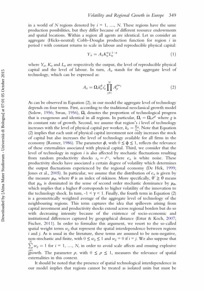
in a world of N regions denoted by i = 1, …, N. These regions have the sameproduction possibilities, but they differ because of different resource endowmentsand spatial locations. Within a region all agents are identical. Let us consider anaggregate (Hicks-neutral) Cobb–Douglas production function for region i inperiod t with constant returns to scale in labour and reproducible physical capital:

Yit ¼ AitKait L

1�ait ð1Þ

where Yit, Kit and Lit are respectively the output, the level of reproducible physicalcapital and the level of labour. In turn, Ait stands for the aggregate level oftechnology, which can be expressed as:

Ait ¼ Xtk/it s

cit

YNj 6¼i

Aqwij

jt ð2Þ

As can be observed in Equation (2), in our model the aggregate level of technologydepends on four terms. First, according to the traditional neoclassical growth model(Solow, 1956; Swan, 1956), Ωt denotes the proportion of technological progressthat is exogenous and identical in all regions. In particular, Xt ¼ X0egt where g isits constant rate of growth. Second, we assume that region’s i level of technologyincreases with the level of physical capital per worker, kit ¼ Kit

Lit. Note that Equation

(2) implies that each unit of physical capital investment not only increases the stockof capital but also increases the level of technology available for all firms in theeconomy (Romer, 1986). The parameter ϕ, with 0 ≤ ϕ ≤ 1, reflects the relevanceof these externalities associated with physical capital. Third, we consider that thelevel of technology in region i is also affected by stochastic fluctuations resultingfrom random productivity shocks sit ¼ eEit , where ϵit is white noise. Theseproductivity shocks have associated a certain degree of volatility which determinesthe output fluctuations experienced by the regional economy (De Hek, 1999;Jones et al., 2005). In particular, we assume that the distribution of ϵit is given bythe measure μθ, where θ is an index of riskiness. More specifically, θʹ ≥ θ meansthat lh0 is dominated in the sense of second order stochastic dominance by μθ,which implies that a higher θ corresponds to higher volatility of the innovation tothe technology shock. In turn, -1 < γ < 1. Finally, the fourth term in Equation (2)is a geometrically weighted average of the aggregate level of technology of theneighbouring regions. This term captures the idea that spillovers arising fromcapital investment and productivity shocks extend across regional borders but do sowith decreasing intensity because of the existence of socio-economic andinstitutional differences captured by geographical distance (Ertur & Koch, 2007;Fischer, 2011). In order to formalize this argument, we resort to the so-calledspatial weight terms wij that represent the spatial interdependence between regionsi and j. As is usual in the literature, these terms are assumed to be non-negative,non-stochastic and finite, with 0 ≤ wij ≤ 1 and wij = 0 if i = j. We also suppose thatPNj 6¼i

wij ¼ 1 for i = 1, …, N, in order to avoid scale affects and ensuing explosive

growth. The parameter ρ, with 0 ≤ ρ ≤ 1, measures the relevance of spatialexternalities in this context.

It should be noted that the presence of spatial technological interdependence inour model implies that regions cannot be treated as isolated units but must be


Dow

nloa

ded

by [

Alm

a M

ater

Stu

dior

um -

Uni

vers

ità d

i Bol

ogna

] at

07:

01 0

5 O

ctob

er 2

015

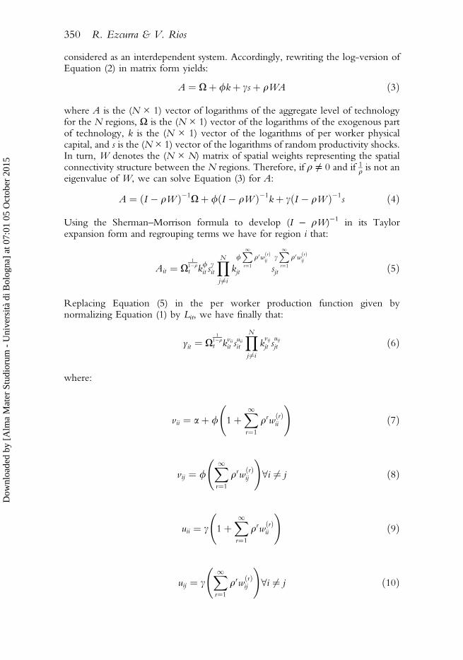
considered as an interdependent system. Accordingly, rewriting the log-version ofEquation (2) in matrix form yields:

A ¼ Xþ /kþ csþ qWA ð3Þ

where A is the (N × 1) vector of logarithms of the aggregate level of technologyfor the N regions, Ω is the (N × 1) vector of the logarithms of the exogenous partof technology, k is the (N × 1) vector of the logarithms of per worker physicalcapital, and s is the (N × 1) vector of the logarithms of random productivity shocks.In turn, W denotes the (N × N) matrix of spatial weights representing the spatialconnectivity structure between the N regions. Therefore, if ρ ≠ 0 and if 1

q is not aneigenvalue of W, we can solve Equation (3) for A:

A ¼ ðI � qW Þ�1Xþ /ðI � qW Þ�1kþ cðI � qW Þ�1s ð4Þ

Using the Sherman–Morrison formula to develop (I − ρW)−1 in its Taylorexpansion form and regrouping terms we have for region i that:

Ait ¼ X1

1�qt k/it s

cit

YNj 6¼i

k/P1r¼1

qrwðrÞij

jt scP1r¼1

qrwðrÞij

jt ð5Þ

Replacing Equation (5) in the per worker production function given bynormalizing Equation (1) by Lit, we have finally that:

yit ¼ X1

1�qt kviiit s

uiiit

YNj 6¼i

kvijjt s

uijjt ð6Þ

where:

vii ¼ aþ / 1þX1r¼1

qrwðrÞii

!ð7Þ

vij ¼ /X1r¼1

qrwðrÞij

!8i 6¼ j ð8Þ

uii ¼ c 1þX1r¼1

qrwðrÞii

!ð9Þ

uij ¼ cX1r¼1

qrwðrÞij

!8i 6¼ j ð10Þ


Dow

nloa

ded

by [

Alm

a M

ater

Stu

dior

um -

Uni

vers

ità d

i Bol

ogna

] at

07:

01 0

5 O

ctob

er 2

015

Given the production function, at each date t the representative agent of region imust choose how much to invest, xit, and consume, cit, in order to maximize herexpected overall utility. Assuming that physical capital fully depreciates eachperiod, the agent faces the following dynamic optimization problem (De Hek,1999):

MaxX1t¼0

dtEU citð Þ ð11Þ

subject to

cit þ kitþ1 ¼ yit

yit ¼ X1

1�qt kviiit s

uiiit

YNj 6¼i

kvijjt s

uijjt

cit � 0; xit � 0; ki0 given

where the parameter δ stands for the discount factor, with 0 < δ < 1. In turn, thepreferences are represented by a constant elasticity of substitution utility function:

uðcitÞ ¼ c1�rit � 11� r

ð12Þ

with σ ≠ 1, σ > 0.The first-order conditions for consumption and investment are given by the

following set of equations:

cit½ � : dt c�rit ¼ kt ð13Þ

kitþ1½ � : �kt þ ktþ1 viiX1

1�q

tþ1suiiitþ1k

vii�1itþ1

YNj 6¼i

suijjt k

vijjtþ1

!¼ 0 ð14Þ

where λt is the Lagrange multiplier at time t. Combining Equations (13) and (14),we can obtain the following Euler equation:

1 ¼ dEcitcitþ1

� �r

viiX1

1�q

tþ1suiiitþ1k

vii�1itþ1

YNj 6¼i

suijjt k

vijjtþ1

!" #ð15Þ


Dow

nloa

ded

by [

Alm

a M

ater

Stu

dior

um -

Uni

vers

ità d

i Bol

ogna

] at

07:

01 0

5 O

ctob

er 2

015

Therefore the expected value of the growth rate of region i between t and t + 1 isgiven by:

Eyitþ1

yit

� �¼ dviið ÞE X

1�r1�q

itþ1kvii�1itþ1 s

gitþ1

YNj 6¼i

kð1�rÞvijjtþ1 sfjtþ1

!" #1r

X1

1�qsuiiitþ1

YNj 6¼i

kvijjtþ1s

uijjtþ1

!

ð16Þ

where g ¼ ð1� rÞuii and f ¼ ð1� rÞuij.We are interested in the effect of increasing volatility of the random productivity

shocks on the decision variables of the model and the resulting expected growthrate. To that end, let us consider the following function of η and ζ:

H g; fð Þ ¼ E suiiitþ1; suijjtþ1

� �h iE sgitþ1; s

fjtþ1

� �h i1r ð17Þ

Note that the impact of a change in volatility on the expected growth rate isdetermined by the effect of a change in volatility on H g; fð Þ. According toEquation (17), there are two channels through which volatility can affect theexpected growth rate. The first channel is related to the learning by doing effect

given by the function E suiiitþ1; suijjtþ1

� �, while the second channel has to do with the

optimal savings rate function E sgitþ1; sfjtþ1

� �h i1r. In order to analyze the effect of a

change in volatility on the expected growth rate, we need to determine the shapeof the functions associated with each channel. Focusing on the learning by doingchannel, Equation (17) indicates that the impact on the expected growth rate ofregion i of an increase in the degree of volatility experienced by the own region ispositive when uit > 1, null if uit = 1 and negative when 0 < uit < 1. Furthermore,an increasing volatility in the neighbouring regions exerts a positive effect on theexpected growth rate of region i when uij > 1, null if uij = 1 and negative when0 < uij < 1. Regarding the channel related to the optimal saving rate, Equation (17)shows that the impact on the expected growth rate of region i of an increase in thedegree of volatility experienced by the own region is positive when η > 1, null ifη = 1 and negative when 0 < η < 1. Additionally, an increasing volatility in theneighbouring regions has a positive effect on the expected growth rate of region iwhen ζ > 1, null if ζ = 1 and negative when ζ < 1.

As can be observed, our model shows that the final impact of volatility onregional growth rates is theoretically ambiguous. Empirical research is therefore keyto shed further light on the relationship between business cycle fluctuations andregional economic growth. For this reason, the rest of the paper is devoted tostudying empirically this issue using data for the European regions.

4. Empirical Framework

4.1. Data

The data for our empirical analysis are drawn from the Cambridge Econometricsregional database and Eurostat. In order to maximize the number of countriesincluded in the analysis, the study period goes from 1991 to 2011. The sample


Dow

nloa

ded

by [

Alm

a M

ater

Stu

dior

um -

Uni

vers

ità d

i Bol

ogna

] at

07:

01 0

5 O

ctob

er 2

015

covers a total of 272 NUTS-2 regions belonging to 27 EU member states, as wellas Norway.4 NUTS-2 regions are used in the analysis instead of other possiblealternatives for various reasons. First, NUTS-2 is the territorial unit mostcommonly employed in the literature to investigate the determinants of regionalgrowth in Europe, which facilitates the comparison of our results with thoseobtained in previous papers. Second, NUTS-2 regions are particularly relevant interms of the EU regional policy since the 1989 reform of the European StructuralFunds. The definitions of all the variables used in the analysis and their specificsources are presented in the Appendix.

4.2. Econometric Model

As mentioned in the introduction, earlier studies on the volatility–growthconnection in the European regions use a cross-sectional approach (Martin &Rogers, 2000; Falk & Sinabell, 2009). Nevertheless, the nature of our datasetallows us to employ panel data techniques in this context, thus extendingmodelling possibilities as compared to the single equation cross-sectional settingemployed so far. In view of this, we begin by considering in our empirical analysisthe following fixed-effects model:

DYit ¼ ai þ Xitbþ eit ð18Þ

where ΔY is the average growth rate of GDP per capita in region i measured overfive-year periods, X is a vector that includes the standard deviation of regionalgrowth rates over each five-year period as a measure of volatility, as well as a set ofadditional variables that control for other factors that are assumed to influenceregional growth. In turn, α stands for unobservable region-specific effects, whereasε represents the corresponding disturbance term.

The control variables included in vector X have been selected on the basis ofthe findings of existing studies on the determinants of regional growth in Europe.While the choice of these variables is theoretically well grounded, it ultimatelydepends on the availability of reliable statistical data for the geographical setting onwhich our study is focused. Thus, following the convention in the literature oneconomic growth, the initial level of GDP per capita is used to control foreconomic convergence across regions (Barro & Sala-i-Martin, 1992). The inclusionof this variable in the model allows us to determine whether poor regions grewfaster than richer ones during the study period, thus providing information on thedynamics of regional disparities. We also control for the level of investment and thepopulation growth rate of the sample regions, two variables theoretically importantwhen it comes to explaining capital accumulation and economic growth (Mankiwet al., 1992; Barro & Sala-i-Martin, 1995). We also include in vector X the share ofthe active population with tertiary education and/or an employment in science andtechnology as a human capital control.5 This is particularly important, given therelevant role played by investment in human capital when explaining regionalgrowth in Europe (Crespo Cuaresma & Feldkircher, 2013).

Additionally, regional growth patterns may be affected by the possible existenceof agglomeration economies (Ciccone, 2002; Fujita & Thisse, 2002). Agglomera-tion economies result from market and non-market interactions, and imply thatproximity to larger markets leads to productivity gains. In order to capture thedegree of spatial concentration of economic activity in a given area, we add to the


Dow

nloa

ded

by [

Alm

a M

ater

Stu

dior

um -

Uni

vers

ità d

i Bol

ogna

] at

07:

01 0

5 O

ctob

er 2

015

list of regressors of our baseline specification the employment density of the variousregions (Ciccone, 2002). Furthermore, the economic performance of the sampleregions may be related to the sectoral composition of economic activity. Indeed,several studies have found that industry mix affects regional growth in the EU (e.g.Paci & Pigliaru, 1999). Although the European economy has experienced a processof convergence in regional productive structures during the last decades,considerable differences persist in the patterns of regional specialization acrossEurope (Ezcurra et al., 2006). Accordingly, vector X also includes the regionalemployment shares in agriculture, financial services and non-market services.

When examining the volatility–growth link, it is particularly important tocontrol for regional size, as this factor may be related to the intensity of the outputfluctuations experienced by the sample regions. Larger regions are oftencharacterized by lower levels of specialization than smaller regions (Ezcurra et al.,2006), which may imply a greater ability to face the adverse effects of economicshocks (Malizia & Ke, 1993; Trendle, 2006). It should be recalled that the region-specific effects included in our baseline specification allow us to control for thosetime-invariant factors relevant in this context. This is the case of region’s area.Nevertheless, we checked that the correlation coefficient between these region-specific effects and total population (an alternative measure of regional size) isrelatively low (ρ = 0.06). In view of this, we opt to add region’s population as anadditional regressor in Equation (18).

With the only exception of the population growth rate, all the explanatoryvariables included in vector X are measured at the beginning of each subperiod inorder to minimize any potential endogeneity problem. Table A1 in the Appendixprovides some descriptive statistics for the different variables.

At this point it is important to note that, as is usual in the traditionalconvergence literature, Equation (18) considers the various regions as isolated units,thus ignoring the spatial characteristics of the data and the potential role ofgeography in shaping economic growth (Rey & Janikas, 2005). This should raiseno major problems, as long as each economy evolves independently of the rest.However, this does not seem a very realistic assumption in the context of theeconomic integration process currently underway in Europe. On the contrary, theimportance of interregional trade, migratory movements and technology andknowledge transfer processes suggests that geographical location may play animportant role in explaining regional growth patterns in the European setting(López-Bazo et al., 2004; Fingleton & López-Bazo, 2006). In fact, the theoreticalmodel developed in Section 3 shows that regional growth rates may be affected bythe degree of volatility experienced by neighbouring regions. The consequences ofomitting these spatial effects from the specification of Equation (18) are potentiallyimportant from an econometric perspective (Anselin, 1988). Accordingly, weshould take into account this potential problem in our empirical analysis. At thispoint it is important to note that our theoretical model does not provide a specificspatial specification to be estimated. In view of this, we begin by considering afixed-effects spatial Durbin model, which is sufficiently general to allow fordifferent types of spatial interactions between the sample regions. This model canbe written as follows:

DYit ¼ ai þ qWDYit þ XitbþWXithþ tit ð19Þ


Dow

nloa

ded

by [

Alm

a M

ater

Stu

dior

um -

Uni

vers

ità d

i Bol

ogna

] at

07:

01 0

5 O

ctob

er 2

015

where W is the spatial weights matrix used to capture the degree of spatialinterdependence between the various regions, and ν is the disturbance term. As canbe observed, in this specification the regional growth rates depend on the spatial lagof the dependent variable, WΔY, which captures the spatial effects workingthrough the dependent variable. In addition, the model also includes the spatial lagof the measure of volatility and of the rest of control variables, WX.

The presence of spatial lags of the dependent and explanatory variablescomplicates the interpretation of the parameters in Equation (19) (Le Gallo et al.,2003; Anselin & Le Gallo, 2006). Therefore, some caution is required wheninterpreting the estimated coefficients in the spatial Durbin model. As shown byLeSage & Pace (2009, pp. 33–42), in a spatial Durbin model a change in a particularexplanatory variable in region i has a direct effect on that region, but also an indirecteffect on the remaining regions. In our context, the direct effect captures the averagechange in the economic growth rate of a particular region caused by a one unitchange in that region’s explanatory variable. In turn, the indirect effect can beinterpreted as the aggregate impact on the growth rate of a specific region of thechange in an explanatory variable in all other regions, or alternatively as the impactof changing an explanatory variable in a particular region on the growth rates of theremaining regions. LeSage & Pace (2009) show that the numerical magnitudes ofthese two calculations of the indirect effect are identical due to symmetries incomputation. Finally, the total effect is the sum of the direct and indirect impacts.

The specification in Equation (19) is particularly useful in our context, becausethe spatial Durbin model allows one to estimate consistently the effect of volatilityon regional growth when endogeneity is induced by the omission of a (spatiallyautoregressive) variable. Indeed, LeSage & Pace (2009) show that if an unobservedor unknown but relevant variable following a first-order autoregressive process isomitted from the model, the spatial Durbin model produces unbiased coefficientestimates. Additionally, this model does not impose prior restrictions on themagnitude of potential spillover effects. Furthermore, the spatial Durbin model isan attractive starting point for spatial econometric modelling because it includes asspecial cases two alternative specifications widely used in the literature: the spatiallag model and the spatial error model. As can be checked, the spatial Durbin modelcan be simplified to the spatial lag model when θ = 0:

DYit ¼ ai þ qWDYit þ Xitbþ tit ð20Þ

and to the spatial error model if hþ qb ¼ 0:

DYit ¼ ai þ Xitbþ Eit ð21Þ

where Eit ¼ nW Eit þ tit and tit ~ i:i:d: In fact, the spatial Durbin model producesunbiased coefficient estimates even when the true data-generation process is aspatial lag or a spatial error model.

4.3. The Spatial Weights Matrix

The estimation of the various spatial models described above requires to definepreviously a spatial weights matrix. Given that this is a critical issue in spatialeconometric modelling (Corrado & Fingleton, 2012), we consider a broad range ofalternative specifications ofW. Thus, we begin by constructing a spatial weights matrix


Dow

nloa

ded

by [

Alm

a M

ater

Stu

dior

um -

Uni

vers

ità d

i Bol

ogna

] at

07:

01 0

5 O

ctob

er 2

015

based on the concept of first-order contiguity, according to which wij = 1 if regions iand j are physically adjacent and 0 otherwise. We next consider several matrices basedon the k-nearest neighbours (k = 5, 10, 15, 20) computed from the great circledistance between the centroids of the various regions (Le Gallo & Ertur, 2003).Additionally, we construct various inverse distance matrices with different cut-offvalues above which spatial interactions are assumed negligible. As an alternative, wealso consider inverse distance and exponential distance decay matrices whose off-diagonal elements are defined by wij ¼ 1

daijfor a ¼ 1:25; 1:50; . . . ; 3:00 and wij ¼

expð�hdijÞ for h ¼ 0:005; . . . ; 0:030, respectively (Keller & Shiue, 2007; Elhorstet al., 2013). As can be observed, the different matrices described above are based in allcases on the geographical distance between the sample regions, which in itself is strictlyexogenous. This is consistent with the recommendation of Anselin & Bera (1998) andallows us to avoid the identification problems raised by Manski (1993). Furthermore,as is common practice in applied research, all the matrices are row-standardized, so thatit is relative, and not absolute, distance which matters.

In the literature there are different criteria to determine the spatial weightsmatrix that best describe the data. The most widely used approach is to comparethe log-likelihood function values. Nevertheless, this approach has been criticizedbecause it only finds a local maximum among competing models and it may be thecase that the correctly specified W is not included (Harris et al., 2011; Vega &Elhorst, 2013). As an alternative criterion, LeSage & Pace (2009) propose theemployment of the Bayesian posterior model probability, while Elhorst et al.(2013) suggest to select the model with the lowest parameter estimate of theresidual variance. Table 2 shows that, according to these criteria, the mostappropriate matrix in our context is the exponential distance decay W with θ =0.01. Therefore, this is the spatial weights matrix used in the rest of the paper.

Table 2. Spatial weights matrix selection

Bayesian posterior modelprobability

Log-likelihood functionvalue

Residualvariance

First-order contiguity 1.00 3,509.84 1.18E-045-nearest neighbours 0.00 3,552.87 1.09E-0410-nearest neighbours 0.86 3,551.59 1.09E-0415-nearest neighbours 0.00 3,512.16 1.17E-0420-nearest neighbours 0.00 3,466.42 1.28E-04Cut-off500km 1.00 3,564.08 1.07E-04Cut-off 1,000 km 0.00 3,491.27 1.22E-04Cut-off 1,500 km 0.00 3,438.74 1.34E-04Cut-off 2,000 km 0.00 3,401.29 1.44E-041/dα, α = 1.25 0.00 3,411.19 1.41E-041/dα, α = 1.50 0.00 3,447.64 1.32E-041/dα, α = 1.75 0.00 3,481.37 1.24E-041/dα, α = 2.00 0.72 3,526.97 1.14E-041/dα, α = 2.25 0.27 3,533.47 1.13E-041/dα, α = 2.50 0.00 3,535.66 1.12E-041/dα, α = 2.75 0.00 3,540.96 1.11E-041/dα, α = 3.00 0.00 3,532.95 1.13E-04exp(−θd), θ = 0.005 0.00 3,534.70 1.12E-04exp(−θd), θ = 0.010 1.00 3,580.55 1.03E-04exp(−θd), θ = 0.015 0.00 3,579.38 1.04E-04exp(−θd), θ = 0.020 0.00 3,564.39 1.06E-04exp(−θd), θ = 0.030 0.00 3,540.31 1.11E-04


Dow

nloa

ded

by [

Alm

a M

ater

Stu

dior

um -

Uni

vers

ità d

i Bol

ogna

] at

07:

01 0

5 O

ctob

er 2

015

5. Results

5.1. Main Findings

The first column of Table 3 presents the results obtained when the fixed-effectsmodel described in Equation (18) is estimated by ordinary least squares (OLS)assuming that the disturbances are independent and identically distributed. As canbe observed, the coefficient of the standard deviation of regional growth rates isnegative and statistically significant at the 1% level. This seems to indicate theexistence of a negative relationship between volatility and economic growth in theEuropean regions. Furthermore, our results show that the coefficient of initial GDPper capita is negative and statistically significant, indicating the existence of aprocess of conditional convergence across the sample regions. Likewise, theremaining control variables included in vector X are in general statisticallysignificant and have the expected signs.

These results should be treated with caution. In particular it is important torecall that, as mentioned above, there are important reasons to believe that spatialeffects play an important role in explaining regional growth patterns in theEuropean setting, which may cause estimates of Equation (18) to become biased,inconsistent and/or inefficient. In order to investigate the relevance of thispotential problem in our sample, we use the residuals of the OLS estimation ofEquation (18) to calculate the Lagrange multiplier tests for the spatial lag model(LM-LAG) and the spatial error model (LM-ERR), plus their robust versions.Table 4 reveals that the results of these tests lead in all cases to the rejection of thenull hypothesis of absence of residual spatial dependence. In view of this, we nowestimate the various spatial panel data models described in the previous section bymaximum likelihood, using the MATLAB routines written by Elhorst (2014) andthe bias correction method proposed by Lee & Yu (2010).

Column 2 of Table 3 presents the results from the spatial Durbin model,whereas the spatial lag model and the spatial error model are presented respectivelyin columns 3 and 4. Before continuing it is important to evaluate which is the bestspatial specification in this context. To that end, we calculate two likelihood-ratiotests (LR-SD-LAG and LR-SD-ERR) to find out if the spatial Durbin model canbe simplified respectively to the spatial lag model (H0 : θ = 0) or the spatial errormodel (H0 : θ + ρβ = 0). As can be observed in Table 4, the null hypotheses ofboth tests are rejected. This implies that the spatial Durbin model is the appropriatespecification in this context (Elhorst, 2010).

As mentioned in the previous section, correct interpretation of the parameterestimates in the spatial Durbin model requires to take into account the direct,indirect and total effects associated with changes in the regressors. Table 5 showsthis information. Focusing on the main aim of the paper, our results reveal that therelationship between volatility and economic performance is negative andstatistically significant, thus confirming the empirical evidence provided by ourprevious analysis and by Martin & Rogers (2000). In particular, our estimates showthat lowering the volatility measure by one standard deviation is associated with anincrease in the average growth rate of around 1.6%. Nevertheless, this total effect isthe sum of the direct and indirect impact of volatility on growth. If we consider thedirect effect, Table 5 indicates that an increase in the degree of volatility registeredby a specific region exerts a negative and statistically significant impact on itsgrowth rate. In turn, the indirect effect shows that this increase also influencesnegative and significantly on the growth rates of neighbouring regions. In fact, the


Dow

nloa

ded

by [

Alm

a M

ater

Stu

dior

um -

Uni

vers

ità d

i Bol

ogna

] at

07:

01 0

5 O

ctob

er 2

015

Table 3. Estimation results: volatility and regional growth

Model Non-spatial Spatial Durbin Spatial lag Spatial error

Volatility −0.346*** −0.159*** −0.232*** −0.169***(−21.88) (−8.68) (−13.92) (−9.35)

Initial GDP per capita (logs) −0.092*** −0.133*** −0.085*** −0.129***(−19.29) (−25.10) (−17.86) (−24.77)

Investment 0.038*** 0.003 0.037*** 0.006(3.19) (0.29) (3.20) (0.52)

Population growth −0.019 −0.096* −0.035 −0.054(−0.30) (−1.76) (−0.58) (−1.12)

Human capital 0.165*** −0.001 0.122*** 0.000(9.63) (−0.06) (7.23) (0.01)

Employment density (logs) −0.067*** 0.010 −0.006 0.006(−7.76) (1.06) (−0.66) (0.66)

Agriculture −0.014 −0.026 −0.044** −0.032*(−0.79) (−1.44) (−2.46) (−1.82)

Financial services 0.109*** 0.100*** 0.085*** 0.103***(3.61) (2.98) (2.89) (3.16)

Non-market services 0.088*** 0.001 0.078*** 0.009(4.30) (0.03) (3.93) (0.37)

Population (logs) −0.020 −0.024 −0.046*** −0.019(−1.23) (−1.64) (−2.92) (−1.32)

Neighbours’ volatility 0.068**(2.41)

Neighbours’ initial GDP per capita 0.118***(13.72)

Neighbours’ investment 0.005(0.24)

Neighbours’ population growth −0.054(−0.38)

Neighbour’s human capital 0.102***(3.44)

Neighbours’ employment density −0.034**(−2.19)

Neighbours’ agriculture 0.029(0.98)

Neighbours’ financial services −0.192***(−3.53)

Neighbours’ non-market services −0.012(−0.29)

Neighbours’ population −0.031(−0.99)

Neighbour’s economic growth (ρ) 0.768*** 0.455***(28.93) (17.91)

Spatial autoregressive parameter (ξ) 0.897***(58.12)

Region-specific effects Yes Yes Yes YesAdjusted R2 0.72 0.79 0.71 0.54Log-likelihood 3,188.82 3,580.55 3,345.12 2,467.25Observations 1,088 1,088 1,088 1,088

Notes: The dependent variable is in all cases the average growth rate of GDP per capita of the various regionsmeasured over five-year periods.t-statistics in parentheses.*Significant at 10% level, **significant at 5% level, ***significant at 1% level.


Dow

nloa

ded

by [

Alm

a M

ater

Stu

dior

um -

Uni

vers

ità d

i Bol

ogna

] at

07:

01 0

5 O

ctob

er 2

015

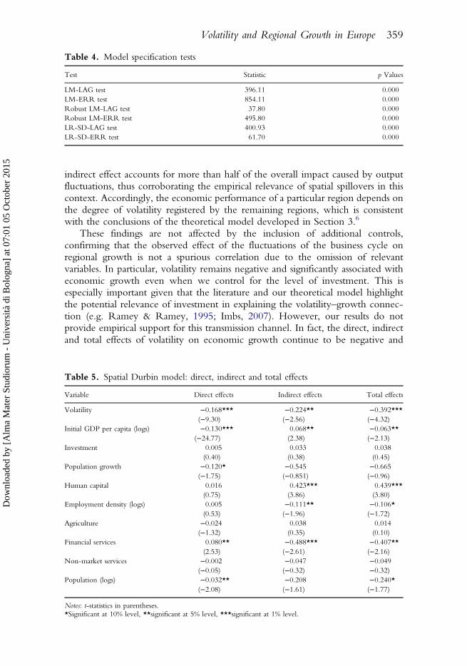
indirect effect accounts for more than half of the overall impact caused by outputfluctuations, thus corroborating the empirical relevance of spatial spillovers in thiscontext. Accordingly, the economic performance of a particular region depends onthe degree of volatility registered by the remaining regions, which is consistentwith the conclusions of the theoretical model developed in Section 3.6

These findings are not affected by the inclusion of additional controls,confirming that the observed effect of the fluctuations of the business cycle onregional growth is not a spurious correlation due to the omission of relevantvariables. In particular, volatility remains negative and significantly associated witheconomic growth even when we control for the level of investment. This isespecially important given that the literature and our theoretical model highlightthe potential relevance of investment in explaining the volatility–growth connec-tion (e.g. Ramey & Ramey, 1995; Imbs, 2007). However, our results do notprovide empirical support for this transmission channel. In fact, the direct, indirectand total effects of volatility on economic growth continue to be negative and

Table 4. Model specification tests

Test Statistic p Values

LM-LAG test 396.11 0.000LM-ERR test 854.11 0.000Robust LM-LAG test 37.80 0.000Robust LM-ERR test 495.80 0.000LR-SD-LAG test 400.93 0.000LR-SD-ERR test 61.70 0.000

Table 5. Spatial Durbin model: direct, indirect and total effects

Variable Direct effects Indirect effects Total effects

Volatility −0.168*** −0.224** −0.392***(−9.30) (−2.56) (−4.32)

Initial GDP per capita (logs) −0.130*** 0.068** −0.063**(−24.77) (2.38) (−2.13)

Investment 0.005 0.033 0.038(0.40) (0.38) (0.45)

Population growth −0.120* −0.545 −0.665(−1.75) (−0.851) (−0.96)

Human capital 0.016 0.423*** 0.439***(0.75) (3.86) (3.80)

Employment density (logs) 0.005 −0.111** −0.106*(0.53) (−1.96) (−1.72)

Agriculture −0.024 0.038 0.014(−1.32) (0.35) (0.10)

Financial services 0.080** −0.488*** −0.407**(2.53) (−2.61) (−2.16)

Non-market services −0.002 −0.047 −0.049(−0.05) (−0.32) −0.32)

Population (logs) −0.032** −0.208 −0.240*(−2.08) (−1.61) (−1.77)

Notes: t-statistics in parentheses.*Significant at 10% level, **significant at 5% level, ***significant at 1% level.


Dow

nloa

ded

by [

Alm

a M

ater

Stu

dior

um -

Uni

vers

ità d

i Bol

ogna

] at

07:

01 0

5 O

ctob

er 2

015

statistically significant when the investment level is excluded from the list ofregressors.

Table 5 also provides interesting information about the different control variablesincluded in vector X. Thus, it should be noted that the direct effect estimates aremostly statistically significant. In particular, the results obtained show that regionswith relatively low levels of GDP per capita tend to grow faster, confirming theexistence of a process of conditional convergence across the European regionsduring the study period. Furthermore, the population growth rate is negativelyassociated with the dependent variable. Likewise, our estimates also reveal that theemployment share in financial services has a positive impact on regional growth,while the impact of total population is negative. These findings are in generalconsistent with the empirical evidence provided by the literature on regional growthin Europe. In turn, the investment level, human capital, employment density andthe employment shares in agriculture and non-market services do not seem to exerta statistically significant direct effect on the dependent variable. In any case, it isimportant to observe that there are variables in which the direct effects displayed inTable 5 tend to be similar to the spatial Durbin model coefficient estimates of thenon-spatial lagged variables reported in the second column of Table 3. Thedifferences between these measures are due to feedback effects that arise from spatialspillovers induced by each region in the whole system. In those cases where thesedifferences are not particularly relevant, we can conclude that feedback effects donot play an important role in this context. Table 5 also reveals that the indirectimpacts are statistically significant for the initial level of GDP per capita, the humancapital control, employment density and the employment share in financial services.This means that the effect on the dependent variable of the remaining controlvariables tends to be confined to the region itself.

As mentioned above, the sum of direct and indirect effects allows one toquantify the total effect on regional growth of the different control variables. Whendirect and indirect effects are jointly taken into account, Table 5 indicates that thetotal effect is statistically significant exclusively in the case of the initial level of GDPper capita, the human capital control, employment density, the employment share infinancial services and total population. The total effect of the initial level of GDP percapita implies a speed of convergence of 3.26%. When interpreting this result, it isinteresting to note that the level of development of neighbouring regions has apositive influence on the growth rate of any given region, thus reducing the speed ofconvergence provided by the estimate of the direct effect of the initial level of GDPper capita. In turn, the investment in human capital exerts a positive influence on theeconomic performance of the European regions, which has to do with the relevanceof spatial spillovers associated with this variable. In the case of employment densityand the employment share in financial services, the negative indirect effectsoutweigh the positive direct effects. As a result, the total effects of these variablesshow a negative correlation between them and the dependent variable. Further-more, smaller regions are characterized by registering higher growth rates,confirming the information provided by the direct effect.

5.2. Robustness Checks

The analysis carried out so far suggests the existence of a negative and statisticallysignificant link between the intensity of output fluctuations and regional growth in


Dow

nloa

ded

by [

Alm

a M

ater

Stu

dior

um -

Uni

vers

ità d

i Bol

ogna

] at

07:

01 0

5 O

ctob

er 2

015

Europe. In particular, our estimates seem to indicate that the observed relationshipis in part due to the existence of spatial spillovers induced by volatility inneighbouring regions. In the rest of this section we investigate the robustness ofthese findings.

As a first robustness test, we examine to what extent our results may besensitive to the choice of the measure used to quantify the incidence of volatility inour sample regions. To that end, we resort to an alternative measure of volatilityused in the real business cycle literature that consists of the standard deviation of theGDP per capita gap (Hnatkovska & Loayza, 2004). To calculate this measure, thetrend of each region’s GDP per capita series is estimated by applying the Hodrick–Prescott filter. The standard deviation of GDP per capita growth employed so farin the paper is based on the implicit assumption that the trend of GDP grows at aconstant rate, whereas this measure allows the trend of GDP to follow a richer,time- and regional-dependant process. Table 6 shows the direct, indirect and totaleffects obtained when the spatial Durbin model is estimated using the standarddeviation of the GDP per capita gap to capture the relevance of the fluctuations ofthe business cycle in the sample regions. As can be seen, the different effects ofvolatility on regional growth continue to be negative and statistically significant inall cases, confirming our previous results.

We now examine to what extent our findings are contingent on the specificspatial model used to investigate the link between volatility and economic growthin the European regions. In fact, the analysis performed so far is based on theestimation of a spatial Durbin model. As discussed in Section 4, in our particularcontext there are important reasons to justify the employment of the spatial Durbinmodel as our baseline specification. Nevertheless, it is important to note that thespatial Durbin model is a global spillover specification (LeSage, 2014). In view of

Table 6. Robustness analysis (I): an alternative measure of volatility


Volatility −0.241*** −0.250*** −0.492***(−14.52) (−3.16) (−5.99)

Initial GDP per capita (logs) −0.116*** 0.072*** −0.044(−23.84) (2.69) (−1.58)

Investment 0.012 −0.002 0.010(1.14) (−0.03) (0.14)

Population growth −0.154*** −0.712 −0.866(−2.44) (−1.23) (−1.39)

Human capital 0.016 0.328*** 0.345***(0.85) (3.54) (3.54)

Employment density (logs) −0.001 −0.099* −0.100*(−0.13) (−1.92) (−1.86)

Agriculture −0.003 0.050 0.047(−0.16) (0.53) (0.48)

Financial services 0.074** −0.488*** −0.414**(2.43) (−2.94) (−2.47)

Non-market services 0.011 −0.095 −0.084(0.52) (−0.78) (−0.68)

Population (logs) −0.018 −0.139 −0.157(−1.29) (−1.22) (−1.32)



Dow

nloa

ded

by [

Alm

a M

ater

Stu

dior

um -

Uni

vers

ità d

i Bol

ogna

] at

07:

01 0

5 O

ctob

er 2

015

this, and in order to complement our previous results, we now consider two localspatial spillover specifications: the spatial lag of X model (SLX) and the spatialDurbin error model (SDEM), which can be written respectively as follows:

DYit ¼ ai þ XitbþWXithþ tit ð22Þ

and

DYit ¼ ai þ XitbþWXithþ Eit ð23Þ

where Eit ¼ nW Eit þ tit and tit~i:i:d: The results obtained when these alternativespecifications are used instead of the spatial Durbin model are shown in Table 7. Ascan be checked, our main findings remain unaltered. The direct, indirect and totaleffects of volatility on economic growth are negative and statistically significant inall cases, regardless of the spatial model considered.

When interpreting our previous results, it should be noted that the impact ofvolatility on economic growth may differ across regions, depending on their level ofdevelopment. According to this hypothesis, the negative correlation observedbetween volatility and economic performance may be caused by the inclusion in thesample of regions with different levels of economic development. In order to testwhether this is the case, we divide the sample regions into two groups: (i) regionswith a GDP per capita below the 75% of the sample mean at the beginning of eachfive-year period and (ii) remaining regions. This regional classification is used toestimate an alternative version of Equation (19) that allows the volatility–growth

Table 7. Robustness analysis (II): alternative spatial specifications

Model SLX SDEM

Variable Direct effectsIndirecteffects Total effects Direct effects

Indirecteffects

Totaleffects

Volatility −0.167*** −0.237*** −0.403*** −0.177*** −0.153*** −0.330***(−7.91) (−8.12) (−17.31) (−9.67) (−2.96) (−5.76)

Initial GDP percapita (logs)

−0.133*** 0.056*** −0.077*** −0.129*** 0.026* −0.103***(−22.39) (6.03) (−10.18) (−24.30) (1.69) (−6.17)

Investment 0.004 0.008 0.012 0.009 0.058 0.068(0.33) (0.33) (0.57) (0.80) (1.51) (1.59)

Population growth −0.142** −0.167 −0.308* −0.102 −0.141 −0.242(−2.27) (−1.06) (−1.74) (−1.57) (−0.61) (−0.88)

Human capital 0.026 0.293*** 0.319*** 0.036* 0.209*** 0.245***(1.14) (8.93) (11.93) (1.77) (4.69) (4.45)

Employmentdensity (logs)

0.07 −0.118*** −0.110*** 0.006 −0.059** −0.053*(0.72) (−6.62) (−6.91) (0.59) (−2.12) (−1.72)

Agriculture −0.022 −0.028 −0.050* −0.021 0.021 0.000(−1.10) (−0.84) (−1.81) (−1.11) (0.36) (0.00)

Financial services 0.088** −0.233*** −0.145*** 0.092*** −0.178* −0.086(2.25) (−3.71) (−3.17) (2.82) (−1.75) (−0.81)

Non-market services 0.013 −0.009 0.004 0.011 0.065 0.075(0.47) (−0.20) (0.10) (0.50) (0.93) (1.07)

Population (logs) −0.024 −0.091** −0.115*** −0.031** −0.053 −0.084(−1.45) (−2.56) (−3.45) (−2.00) (−1.07) (−1.51)



Dow

nloa

ded

by [

Alm

a M

ater

Stu

dior

um -

Uni

vers

ità d

i Bol

ogna

] at

07:

01 0

5 O

ctob

er 2

015

relationship to be different across groups (Ertur et al., 2006).7 The results of thisadditional analysis are summarized in Table 8. As can be observed, the negativeassociation between volatility and economic performance still holds in the twogroups of regions. Nevertheless, the different effects shown in Table 8 arestatistically significant at conventional levels only in the case of the low-incomeregions. This result is potentially important from a policy perspective, as it suggeststhat output fluctuations are particularly harmful for economic growth in theEurope’s poorest regions.

Finally, we examine whether our results are affected by the fluctuations in theexchange rates of the various countries.8 As pointed out by Bivand & Brunstad(2006, p. 284), regions in countries with unusual exchange rate series can performdifferently from regions in countries with typical exchange rate series. This ispotentially important in our context, since the variations in the exchange rate seriesmay have influence on the values of the regional growth rates and the measure ofvolatility used in our econometric analysis. In order to investigate this issue, wehave adopted an approach similar to that used by Bivand & Brunstad (2006). Inparticular, we have included in our baseline specification a dummy variable thatallows us to identify regions in countries with high fluctuations in the exchangerate series over the study period. This dummy variable takes the value one if theregion is in a country where the standard deviation of the variation of the exchangerate in each five-year period is above the third quartile of the distribution, zerootherwise. As can be observed in Table 9, the total effect on the dependentvariable of this dummy variable is not statistically significant at conventional levels.However, our previous findings on the relationship between volatility andeconomic growth remains unaffected.

Table 8. Robustness analysis (III): the effect of regional development level


Volatility of poorest regions −0.172*** −0.221** −0.393***(−9.33) (−2.18) (−3.74)

Volatility of remaining regions −0.082* −0.315 −0.397(−1.74) (−0.87) (−1.05)


Investment 0.006 0.033 0.039(0.49) (0.38) (0.43)

Population growth −0.122* −0.548 −0.669(−1.75) (−0.81) (−0.93)

Human capital 0.015 0.421*** 0.436***(0.74) (4.00) (3.96)

Employment density (logs) 0.004 −0.106* −0.101(0.46) (−1.77) (−1.63)

Agriculture −0.023 0.037 0.015(−1.22) (0.33) (0.12)

Financial services 0.081** −0.483** −0.402**(2.49) (−2.49) (−2.05)

Non-market services 0.003 −0.051 −0.049(0.11) (−0.37) (−0.34)

Population (logs) −0.031** −0.215 −0.246*(−1.99) (−1.64) (−1.78)



Dow

nloa

ded

by [

Alm

a M

ater

Stu

dior

um -

Uni

vers

ità d

i Bol

ogna

] at

07:

01 0

5 O

ctob

er 2

015

6. Conclusions

This paper has examined the relationship between output volatility and regionalgrowth in Europe. To that end, we have developed a spatially augmented stochasticgrowth model with technological interdependence among economies. Spatialexternalities are used to model technological interdependence, which ultimatelyimplies that the economic growth rate of a particular region is affected not only byits own degree of volatility but also by the output fluctuations registered by theremaining regions.

In order to investigate the empirical validity of this result, we have examinedthe volatility–growth connection in a sample of 272 European regions over theperiod 1991–2011. To do so we have estimated a panel data model using spatialeconometric techniques that allow one to take into account the relevance of spatialeffects in the processes of regional growth. Our estimates show the existence of anegative and statistically significant relationship between volatility and economicgrowth in the European regions. This is partly due to the role played in thiscontext by spatial spillovers induced by volatility in neighbouring regions. Theobserved link is robust to the inclusion in the analysis of different explanatoryvariables that may affect regional growth such as the initial GDP per capita, thelevel of investment and human capital, employment density or industry mix. Wehave also checked that our results do not depend on the measure of volatility usedin the analysis. Likewise, the negative link detected between output fluctuationsand economic growth still holds when alternative econometric specifications areemployed to capture the nature of spatial spillovers in this context.

Table 9. Robustness analysis (IV): the impact of exchange rate fluctuations


Volatility −0.177*** −0.186** −0.363***(−9.53) (−1.96) (−3.65)


Investment 0.006 0.033 0.039(0.57) (0.38) (0.44)

Population growth −0.106 −0.584 −0.691(−1.53) (−0.86) (−0.95)

Human capital 0.014 0.454*** 0.468***(0.68) (4.15) (4.11)

Employment density (logs) 0.006 −0.121** −0.115*(0.69) (−2.01) (−1.83)

Agriculture −0.023 0.055 0.032(−1.25) (0.47) (0.27)

Financial services 0.075** −0.490** −0.415**(2.26) (−2.51) (−2.10)

Non-market services −0.006 −0.057 −0.063(−0.25) (−0.38) (−0.41)

Population (logs) −0.036** −0.199 −0.235*(−2.42) (−1.48) (−1.68)

Exchange rate factor 0.006*** −0.013* −0.007(3.04) (−1.86) (−1.05)



Dow

nloa

ded

by [

Alm

a M

ater

Stu

dior

um -

Uni

vers

ità d

i Bol

ogna

] at

07:

01 0

5 O

ctob

er 2

015

The results obtained in the paper have potentially interesting policy implica-tions. At this point it needs to be recalled that the variability of cyclicalmacroeconomic fluctuations have typically been perceived as a negative phenom-enon. The empirical evidence provided by our analysis confirms this perception. Inparticular, our estimates show that short-term instability is negatively related toregional growth in the European context. This suggests that traditional publicpolicies designed to promote regional growth should be complemented withinitiatives to reduce the business cycle fluctuations experienced by the Europeanregions. In this line, policy-makers could attempt to attract new industries todiversify the regional productive structure, thus reducing the risks faced by thoseregions with an excessive reliance on a small number of economic activities(Ezcurra, 2011). In any case, although further research is required to confirmdefinitely our conclusions, the possible effect of short-term stability on economicgrowth should not be overlooked by policy-makers.

Notes

1. This list of factors is not exhaustive. For further information, see the recent papers by Crespo Cuaresma &Feldkircher (2013) and Crespo Cuaresma et al. (2014), who consider other potential determinants of regionalgrowth in Europe.

2. NUTS is the French acronym for ‘Nomenclature of Territorial Units for Statistics’, a hierarchical classificationof subnational spatial units established by Eurostat according to administrative criteria. In this classification,NUTS-0 corresponds to the country level, while increasing numbers indicate increasing levels of territorialdisaggregation.

3. In addition to these contributions based on aggregate data, Ezcurra (2010) employs sectorally disaggregated datafor six manufacturing activities to investigate the relationship between the fluctuations of the business cycle andoutput growth in the European regions between 1980 and 2006. Furthermore, Chandra (2003) tests thepredictions of the portfolio model of the economy with European regional data. Using different frontierestimation methods, this author provides evidence of the existence of a convex growth-instability frontier forthe more aggregated regions of Europe.

4. The lack of data has obliged us to exclude from the study the French overseas departments and territories, andthe Portuguese islands in the Atlantic.

5. This specific measure was selected due to the lack of data for other alternative indicators. Nevertheless, it isworth noting that the nature of this variable implies that its use as a human capital control may be questionable,which should be taken into account when interpreting our findings.

6. In order to investigate whether the observed relationship between volatility and economic growth is stable overtime, we repeat the estimation of Equation (19) for the periods 1991–2006 and 1996–2011, using threesubperiods of five years in each case. The results are very similar to those described in the text. In fact, the onlynoticeable difference has to do with the direct effect of volatility on economic growth for the period 1996–2011, which is negative but not statistically significant at conventional levels.

7. As an alternative, one may to consider the possibility of estimating Equation (19) separately for two groups ofregions defined according to the level of development at the beginning of the study period. However, thiswould imply to use different spatial weights matrices in the two groups, thus ignoring the spatialinterdependences between them.

8. We would like to thank an anonymous referee for attracting our attention on this issue.

References

Aghion, P. & Howitt, P. (1998) Endogenous Growth Theory, Cambridge, MA, MIT Press.Aghion, P. & Saint-Paul, G. (1998) Virtues of bad times: interaction between productivity growth and economic

fluctuations, Macroeconomic Dynamics, 2, 322–344.Anselin, L. (1988) Spatial Econometrics: Methods and Models, Dordrecht, Kluwer Academic Publishers.Anselin, L. & Bera, A (1998) Spatial dependence in linear regression models with an introduction to spatial

econometrics, in: A. Ullah & D. E. A. Giles (eds) Handbook of Applied Economic Statistics, pp. 237–289. NewYork, Marcel Dekker.


Dow

nloa

ded

by [

Alm

a M

ater

Stu

dior

um -

Uni

vers

ità d

i Bol

ogna

] at

07:

01 0

5 O

ctob

er 2

015

Anselin, L. & Le Gallo, J. (2006) Interpolation of Air quality measures in hedonic house price models: spatialaspects, Spatial Economic Analysis, 1, 31–52.

Badinger, H. (2010) Output volatility and economic growth, Economics Letters, 106, 15–18.Barro, R. J. & Sala-i-Martin, X. (1992) Convergence, Journal of Political Economy, 100, 223–251.Barro, R. J. & Sala-i-Martin, X. (1995) Economic Growth, New York, McGraw-Hill.Beugelsdijk, S. & Van Schaik, T. (2005) Differences in social capital between 54 Western European regions,

Regional Studies, 39, 1053–1064.Bivand, R. & Brunstad, R. (2006) Regional growth in Western Europe: detecting spatial misspecification using

the R environment, Papers in Regional Science, 85, 277–297.Caporale, T. & McKiernan, B. (1996) The relationship between output variability and growth: evidence from

postwar UK data, Scottish Journal of Political Economy, 43, 229–236.Chandra, S. (2003) Regional economy size and the growth-instability frontier: evidence from Europe, Journal of

Regional Science, 43, 95–122.Chatterjee, P. & Shukayev, M. (2006) Are average growth and volatility related? Working Paper No. 2006-24,

Ottawa, ON, Bank of Canada.Ciccone, A. (2002) Agglomeration effects in Europe, European Economic Review, 46, 213–227.Corrado, L. & Fingleton, B. (2012) Where is the economics in spatial econometrics? Journal of Regional Science, 52,

210–239.Crescenzi, R. & Rodríguez-Pose, A. (2008) Infrastructure endowment and investment as determinants of regional

growth in the EU, EIB Papers, 13, 63–101.Crespo Cuaresma, J. & Feldkircher, M. (2013) Spatial filtering, model uncertainty and the speed of income

convergence in Europe spatial filtering and model uncertainty, Journal of Applied Econometrics, 28, 720–741.Crespo Cuaresma, J., Doppelhofer, G. & Feldkircher, M. (2014) The determinants of economic growth in

European regions, Regional Studies, 48, 44–67.Dawson, J. W. & Stephenson, E. F. (1997) The link between volatility and growth: evidence from the states,

Economics Letters, 55, 365–369.De Hek, P. A. (1999) On endogenous growth under uncertainty, International Economic Review, 40, 727–744.Dejuan, J. & Gurr, S. (2004) On the link between volatility and growth: evidence from Canadian provinces,

Applied Economics Letters, 11, 279–282.Elhorst, J. P. (2010) Applied spatial econometrics: raising the bar, Spatial Economic Analysis, 5, 9–28.Elhorst, J. P. (2014) Matlab software for spatial panels, International Regional Science Review, 37, 389–405.Elhorst, J.P., Zandberg E. & De Haan, J. (2013) The impact of interaction effects among neighbouring countries

on financial liberalization and reform: a dynamic spatial panel data approach, Spatial Economic Analysis, 8,293–313.

Ertur, C. & Koch, W. (2007) Growth, technological interdependence and spatial externalities: theory andevidence, Journal of Applied Econometrics, 22, 1033–1062.

Ertur, C., Le Gallo, J. & Baumont, C. (2006) The European regional convergence process, 1980–1995: do spatialregimes and spatial dependence matter? International Regional Science Review, 29, 3–34.

European Commission (2007) Fourth Report on Economic and Social Cohesion: Growing Regions, Growing Europe,Luxembourg, Office for Official Publications of the European Communities.

Ezcurra, R. (2009) Does income polarization affect economic growth? The case of the European regions, RegionalStudies, 43, 267–285.

Ezcurra, R. (2010) Sectoral volatility and regional growth in the European Union, Environment and Planning C:Government and Policy, 28, 369–380.

Ezcurra, R. (2011) Unemployment volatility and regional specialization in the European Union, Regional Studies,45, 1121–1137.

Ezcurra, R., Pascual P. & Rapún, M. (2006) Regional specialization in the European Union, Regional Studies, 40,601–616.

Fagerberg, J., Verspagen B. & Caniëls, M. (1997) Technology, growth and unemployment across Europeanregions, Regional Studies, 31, 457–466.

Falk, M. & Sinabell, F. (2009): A spatial econometric analysis of the regional growth and volatility in Europe,Empirica, 36, 193–207.

Fingleton, B. & López-Bazo, E. (2006) Empirical growth models with spatial effects, Papers in Regional Science, 85,177–199.

Fischer, M. (2011) A spatial Mankiw–Romer–Weil model: theory and evidence, The Annals of Regional Science,47, 419–436.

Fujita, M. & Thisse, J. F. (2002) Economics of Agglomeration, Cambridge, Cambridge University Press.Gil, C., Pascual, P. & Rapún, M. R. (2002) Structural change, infrastructure and convergence in the regions of

the European Union, European Urban and Regional Studies, 9, 115–135.


Dow

nloa

ded

by [

Alm

a M

ater

Stu

dior

um -

Uni

vers

ità d

i Bol

ogna

] at

07:

01 0

5 O

ctob

er 2

015

Grier, K. B. & Tullock, G. (1989) An empirical analysis of cross-national economic growth, 1951–1980, Journal ofMonetary Economics, 24, 259–276.

Harris, R., Moffat J. & Kravtsova, V. (2011) In search of ‘W’, Spatial Economic Analysis, 6, 249–270.Hnatkovska, V. & Loayza, N. (2004) Volatility and growth. World Bank Policy Research Working Paper

No. 3184.Imbs, J. (2007) Growth and volatility, Journal of Monetary Economics, 54, 1848–1862.Islam, N. (2003) What have we learnt from the convergence debate? Journal of Economic Surveys, 17, 309–362.Jones, L., Manuelli, E. & Stacchetti, E. (2005) Neoclassical models of endogenous growth: the effects of fiscal

policy, innovation and fluctuations, in: P. Aghion & S. Durlauf (eds), Handbook of Economic Growth, pp. 13–62,Amsterdam, Elsevier.

Keller, W. & Shiue, C. H. (2007) The origin of spatial interaction, Journal of Econometrics, 140, 304–332.Kormendi, R. C. & Meguire, P. G. (1985) Macroeconomic determinants of growth: cross-country evidence,

Journal of Monetary Economics, 16, 141–163.Krugman, P. (1991) Increasing returns and economic geography, Journal of Political Economy, 99, 483–499.Kydland, F. E. & Prescott, E. C. (1982) Time to build and aggregate fluctuations, Econometrica, 50, 1345–1370.Le Gallo, J. & Dall’erba, S. (2008) Spatial and sectoral productivity convergence between European regions,

1975–2000, Papers in Regional Science, 87, 505–525.Le Gallo, J. & Ertur, C. (2003) Exploratory spatial data analysis of the distribution of regional per capita GDP in

Europe, 1980–1995, Papers in Regional Science, 82, 175–201.Le Gallo, J., Ertur, C. & Baumont, C. (2003) A spatial econometric analysis of convergence across European

regions, 1980–1995, in: B. Fingleton (ed), European Regional Growth, pp. 99–129, Berlin, Springer-Verlag.Lee, L.-F. & Yu, J. (2010) Estimation of spatial autoregressive panel data models with fixed effects, Journal of

Econometrics, 154, 165–185.LeSage, J. P. (2014) What regional scientists need to know about spatial econometrics, The Review of Regional

Studies, 44, 13–32.LeSage J. P. & Pace, R. K. (2009) An Introduction to Spatial Econometrics, Boca Raton, FL, Chapman & Hall.López-Bazo, E., Vayá, E. & Artis, A. (2004) Regional externalities and growth: evidence from European regions,

Journal of Regional Science, 44, 43–73.Malizia, E. E. & Ke, S. (1993) The influence of economic diversity on unemployment and stability, Journal of

Regional Science, 33, 221–235.Mankiw, N. G., Romer D. & Weil, D. N. (1992) A contribution to the empirics of economic growth, The

Quarterly Journal of Economics, 107, 407–437.Manski, C. F. (1993) Identification of endogenous social effects: the reflection problem, The Review of Economic

Studies, 60, 531–542.Martin, P. & Rogers, A. C. (2000) Long-term growth and short-term economic instability, European Economic

Review, 44, 359–381.Norrbin, S. C. & Pinar Yigit, F. (2005) The robustness of the link between volatility and growth of output,

Review of World Economics, 141, 343–356.Paci, R. & Pigliaru, F. (1999) European regional growth: do sectors matter? In: J. Adams & R. Paci (eds), Economic

Growth and Change: Regional and National Patterns of Convergence and Divergence, pp. 213–235, Cheltenham,McGraw-Hill.

Ramey G. & Ramey, V. A. (1995) Cross-country evidence on the link between volatility and growth, AmericanEconomic Review, 85, 1138–1151.

Rey, S. J. & Janikas, M. V. (2005) Regional convergence, inequality, and space, Journal of Economic Geography, 5,155–176.

Rodríguez-Pose, A. & Fratesi U. (2004) Between development and social policies: the impact of Europeanstructural funds in objective 1 regions, Regional Studies, 38, 97–113.

Rodríguez-Pose, A. & Vilalta-Bufi, M. (2005) Education, migration and job satisfaction: the regional returns ofhuman capital in the EU, Journal of Economic Geography, 5, 545–566.

Romer, P. M. (1986) Increasing returns and long run growth, Journal of Political Economy, 94, 1002–1036.Solow, R. M. (1956) A contribution to the theory of economic growth, The Quarterly Journal of Economics, 70,

65–94.Speight, A. E. (1999) UK output volatility and growth: some further evidence, Scottish Journal of Political Economy,

46, 175–184.Swan, T. W. (1956) Economic growth and capital accumulation, Economic Record, 32, 334–361.Trendle, B. (2006) Regional economic instability: the role of industrial diversification and spatial spillovers, The

Annals of Regional Science, 40, 767–778.Vega, S. H. & Elhorst, P. (2013) Modelling regional labour market dynamics in space and time, Papers in Regional

Science, 93, 819–841.


Dow

nloa

ded

by [

Alm

a M

ater

Stu

dior

um -

Uni

vers

ità d

i Bol

ogna

] at

07:

01 0

5 O

ctob

er 2

015

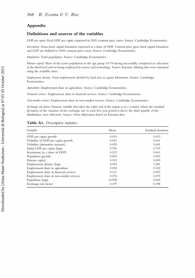
Appendix

Definitions and sources of the variables

GDP per capita: Real GDP per capita expressed in 2005 constant price euros. Source: Cambridge Econometrics.

Investment: Gross fixed capital formation expressed as a share of GDP. Current price gross fixed capital formationand GDP are deflated to 2005 constant price euros. Source: Cambridge Econometrics.

Population: Total population. Source: Cambridge Econometrics.

Human capital: Share of the active population in the age group 15–74 having successfully completed an educationat the third level and/or being employed in science and technology. Source: Eurostat. Missing data were estimatedusing the available series.

Employment density: Total employment divided by land area in square kilometres. Source: CambridgeEconometrics.

Agriculture: Employment share in agriculture. Source: Cambridge Econometrics.

Financial services: Employment share in financial services. Source: Cambridge Econometrics.

Non-market services: Employment share in non-market services. Source: Cambridge Econometrics.

Exchange rate factor: Dummy variable that takes the value one if the region is in a country where the standarddeviation of the variation of the exchange rate in each five-year period is above the third quartile of thedistribution, zero otherwise. Source: Own elaboration based on Eurostat data.

Table A1. Descriptive statistics

Variable Mean Standard deviation

GDP per capita growth 0.014 0.013Volatility of GDP per capita growth 0.031 0.041Volatility (alternative measure) 0.029 0.041Initial GDP per capita (logs) 9.706 0.715Investment (as a share of GDP) 0.213 0.061Population growth 0.003 0.009Human capital 0.315 0.090Employment density (logs) 4.094 1.281Employment share in agriculture 0.090 0.102Employment share in financial services 0.111 0.057Employment share in non-market services 0.274 0.072Population (logs) 14.098 0.836Exchange rate factor 0.197 0.398


Dow

nloa

ded

by [

Alm

a M

ater

Stu

dior

um -

Uni

vers

ità d

i Bol

ogna

] at

07:

01 0

5 O

ctob

er 2

015

Vol Growth Sea Publicado

Documents

Transcript of Vol Growth Sea Publicado