Visual Testing - Aalto University
99
Jan Lönnberg Visual testing of software 7th October 2003 Teknillinen korkeakoulu Helsinki University of Technology Tietotekniikan osasto Department of Computer Science and Engineering
Transcript of Visual Testing - Aalto University
Jan Lönnberg
Visual testing of software
7th October 2003
Teknillinen korkeakoulu Helsinki University of TechnologyTietotekniikan osasto Department of Computer Science and Engineering

i
Helsinki University of TechnologyAbstract of master’s thesis
Author: Jan LönnbergTitle of thesis: Visual testing of softwareDate: 7th October 2003Number of pages: 1+ x+88Department: Department of Computer Science and EngineeringProfessorship: T-106 (Software Technology)Field of study: Software SystemsSupervisor: Lauri MalmiInstructor: Ari Korhonen
Software development is prone to time-consuming and expensive errors. Finding and cor-recting errors in a program (debugging) is usually done by executing the program withdifferent inputs and examining its intermediate and/or final results (testing). The toolsthat are currently available for debugging (debuggers) do not fully make use of poten-tially useful visualisation and interaction techniques.
This thesis presents a new interactive graphical software testing methodology called visualtesting. A programmer can use a visual testing tool to examine and manipulate a runningprogram and its data structures.
Systems with techniques applicable to visual testing in the related domains of debugging,software visualisation and algorithm animation are surveyed. Techniques that are poten-tially useful to visual testing are described, examined and evaluated, and a design for avisual testing tool based on these techniques is presented. The tool combines aspects ofuser-controlled algorithm simulation, high-level data visualisation and visual debugging,and allows easier testing, debugging and understanding of software.
A prototype visual testing tool is presented and evaluated here as a proof of concept forsome of the aspects of visual testing. Finally, some suggestions for future research invisual testing are presented.
Keywords: visual testing, visual debugging, algorithm simulation, algo-rithm animation, debugging

ii
Teknillinen korkeakouluDiplomityön tiivistelmä
Tekijä: Jan LönnbergTyön nimi: Visual testing of softwareTyön nimi suomeksi: Visuaalinen ohjelmistotestausPäivämäärä: 7. lokakuuta 2003Sivuja: 1+x+88Osasto: Tietotekniikan osastoProfessuuri: T-106 (Ohjelmistotekniikka)Pääaine: OhjelmistojärjestelmätValvoja: Lauri MalmiOhjaaja: Ari Korhonen
Ohjelmistojen kehittäminen on altis kalliille ja henkilöaikaa syöville virheille. Virheet et-sitään yleensä suorittamalla ohjelmaa eri syötteillä ja tarkistamalla tuloksien oikeellisuus,eli testaamalla. Nykyiset vianetsintäohjelmat eivät riittävästi hyödynnä visualisaatio- javuorovaikutusmenetelmien tarjoamia mahdollisuuksia.
Tässä diplomityössä esitetään uusi vuorovaikutteinen graafinen ohjelmistotestausmene-telmä nimeltään visuaalinen testaus. Visuaalisen testauksen työkalu tarjoaa ohjelmoijallemahdollisuuden tutkia ja manipuloida ohjelmaa ja sen tietorakenteita.
Läheisistä aihealueista (vianetsinnästä, ohjelmistovisualisoinnista ja algoritmianimaatios-ta) tutkitaan järjestelmiä, jotka tarjoavat hyödyllisiä menetelmiä visuaaliseen testaukseen.Mahdollisesti hyödylliset tekniikat kuvaillaan, tutkitaan ja arvioidaan. Tämän perusteellasuunnitellaan visuaalinen testaustyökalu, joka yhdistää käyttäjän ohjaaman algoritmisi-mulaation, korkeatasoisen tiedon visualisoinnin ja visuaalisen vianetsinnän ja tekee tes-taamisen, vianetsinnän ja ohjelmistojen ymmärtämisen helpommaksi.
Tässä diplomityössä myös esitetään ja arvioidaan prototyyppi visuaalisestä testaustyö-kalusta, jonka tarkoitus on osoittaa osittain visuaalisen testauksen toimivuutta. Lopuksiesitetään muutama ehdotus tulevalle visuaalisen testauksen tutkimukselle.
Avainsanat: visuaalinen testaus, visuaalinen vianetsintä, algoritmisimulaa-tio, algoritmianimaatio, vianetsintä

iii
Tekniska högskolanSammandrag av diplomarbetet
Utfört av: Jan LönnbergArbetets namn: Visual testing of softwareArbetets namn (på svenska): Visuell testning av programvaraDatum: 7 oktober 2003Sidantal: 1+ x+88Avdelning: Avdelningen för datateknikProfessur: T-106 (Programteknik)Huvudämne: ProgramsystemExaminator: Lauri MalmiHandledare: Ari Korhonen
Då man utvecklar programvara råkar man ofta ut för fel som tar mycket tid och pengar attreda ut. Felen spåras och avlägsnas (avlusning eller debugging) vanligen genom att manutför programmet med olika input och kontrollerar resultaten, vilket kallas testning. Debefintliga avlusningsprogrammen utnyttjar inte till fullo alla möjligheter som visualiseringoch interaktion erbjuder.
I detta diplomarbete presenteras ett nytt interaktivt grafiskt testningsförfarande för pro-gramvara som kallas visuell testning. En programmerare kan med ett verktyg för visuelltestning undersöka och manipulera manipulera ett aktivt program och dess datastrukturer.
I diplomarbetet undersöks system i närliggande områden (avlusning, programvaruvisua-lisering och algoritmanimation), och potentiellt användbara tekniker som används i des-sa beskrivs, undersöks och bedöms. På basen av dessa skapas en design för ett visuelltverktyg för testning av programvara. Detta verktyg kombinerar olika aspekter av använ-darkontrollerad algoritmsimulation, datavisualisering på hög abstraktionsnivå och visuellavlusning. Verktyget förenklar testning, avlusning och förståelse av programvara.
En prototyp av det visuella testningsverktyget presenteras och bedöms också i detta arbe-te. Till slut presenteras några förslag för framtida forskning i visuell testning.
Nyckelord: visuell testning, visuell avlusning, algoritmsimulation, algorit-manimation, avlusning

Acknowledgements
This thesis was written at Helsinki University of Technology as a part of the softwarevisualisation research of the Laboratory of Information Processing Science.
I am greatly indebted to my supervisor, Professor Lauri Malmi, for much of the inspi-ration for this thesis and his enthusiastic guidance, without which this thesis would havebeen noticeably less thorough and structured.
I likewise owe much to my instructor, Ari Korhonen, for the support, suggestions andinspiration he has provided. His ideas, methods and work are reflected throughout thisthesis.
I am also grateful to Panu Silvasti for his kind assistance and Markku Rontu for hishelpful suggestions and comments.
Finally, I want to express my gratitude to my parents for their love, support and under-standing. This thesis is dedicated to them.
Otaniemi, 7th October 2003,
Jan Lönnberg
iv

Contents
1 Introduction 11.1 Goal . . . . . . . . . . . . . . . . . . . . . . . . . . . . . . . . . . . . . . 11.2 Proposed solution . . . . . . . . . . . . . . . . . . . . . . . . . . . . . . . 21.3 Thesis outline . . . . . . . . . . . . . . . . . . . . . . . . . . . . . . . . . 2
2 Objectives 32.1 Criteria . . . . . . . . . . . . . . . . . . . . . . . . . . . . . . . . . . . . 32.2 Scope . . . . . . . . . . . . . . . . . . . . . . . . . . . . . . . . . . . . . 4
2.2.1 Target language . . . . . . . . . . . . . . . . . . . . . . . . . . . . 42.2.2 Solution types to consider . . . . . . . . . . . . . . . . . . . . . . 52.2.3 Prototype . . . . . . . . . . . . . . . . . . . . . . . . . . . . . . . 5
3 Related work 63.1 Debugging . . . . . . . . . . . . . . . . . . . . . . . . . . . . . . . . . . . 6
3.1.1 DDD . . . . . . . . . . . . . . . . . . . . . . . . . . . . . . . . . 73.1.2 RetroVue . . . . . . . . . . . . . . . . . . . . . . . . . . . . . . . 73.1.3 ODB . . . . . . . . . . . . . . . . . . . . . . . . . . . . . . . . . 83.1.4 Amethyst . . . . . . . . . . . . . . . . . . . . . . . . . . . . . . . 83.1.5 Lens . . . . . . . . . . . . . . . . . . . . . . . . . . . . . . . . . . 83.1.6 BlueJ . . . . . . . . . . . . . . . . . . . . . . . . . . . . . . . . . 8
3.2 Program visualisation . . . . . . . . . . . . . . . . . . . . . . . . . . . . . 93.2.1 Jeliot . . . . . . . . . . . . . . . . . . . . . . . . . . . . . . . . . 93.2.2 VCC . . . . . . . . . . . . . . . . . . . . . . . . . . . . . . . . . 93.2.3 UWPI . . . . . . . . . . . . . . . . . . . . . . . . . . . . . . . . . 93.2.4 Korsh-LaFollette-Sangwan . . . . . . . . . . . . . . . . . . . . . . 93.2.5 Prosasim . . . . . . . . . . . . . . . . . . . . . . . . . . . . . . . 103.2.6 Leonardo . . . . . . . . . . . . . . . . . . . . . . . . . . . . . . . 103.2.7 VisiVue . . . . . . . . . . . . . . . . . . . . . . . . . . . . . . . . 103.2.8 Pavane . . . . . . . . . . . . . . . . . . . . . . . . . . . . . . . . 103.2.9 DynaLab . . . . . . . . . . . . . . . . . . . . . . . . . . . . . . . 103.2.10 Tarraingím . . . . . . . . . . . . . . . . . . . . . . . . . . . . . . 103.2.11 JAVAVIS . . . . . . . . . . . . . . . . . . . . . . . . . . . . . . . 10
3.3 Algorithm animation and simulation . . . . . . . . . . . . . . . . . . . . . 113.3.1 Matrix . . . . . . . . . . . . . . . . . . . . . . . . . . . . . . . . . 113.3.2 JDSL . . . . . . . . . . . . . . . . . . . . . . . . . . . . . . . . . 113.3.3 Balsa-II . . . . . . . . . . . . . . . . . . . . . . . . . . . . . . . . 113.3.4 Zeus . . . . . . . . . . . . . . . . . . . . . . . . . . . . . . . . . . 113.3.5 AlgAE . . . . . . . . . . . . . . . . . . . . . . . . . . . . . . . . 123.3.6 World-wide algorithm animation . . . . . . . . . . . . . . . . . . . 123.3.7 JAWAA . . . . . . . . . . . . . . . . . . . . . . . . . . . . . . . . 123.3.8 JCAT . . . . . . . . . . . . . . . . . . . . . . . . . . . . . . . . . 123.3.9 JIVE . . . . . . . . . . . . . . . . . . . . . . . . . . . . . . . . . 12
v

CONTENTS vi
3.4 Evaluation . . . . . . . . . . . . . . . . . . . . . . . . . . . . . . . . . . . 123.5 Analysis . . . . . . . . . . . . . . . . . . . . . . . . . . . . . . . . . . . . 12
3.5.1 Traditional grouping . . . . . . . . . . . . . . . . . . . . . . . . . 143.5.2 Grouping by data extraction approach and code preprocessing . . . 153.5.3 Grouping by view control style . . . . . . . . . . . . . . . . . . . . 163.5.4 Conclusions . . . . . . . . . . . . . . . . . . . . . . . . . . . . . . 17
4 Visualisation 184.1 Primitive value representations . . . . . . . . . . . . . . . . . . . . . . . . 18
4.1.1 Textual representation . . . . . . . . . . . . . . . . . . . . . . . . 184.1.2 Graphical representations . . . . . . . . . . . . . . . . . . . . . . . 194.1.3 Evaluation . . . . . . . . . . . . . . . . . . . . . . . . . . . . . . 19
4.2 Array representations . . . . . . . . . . . . . . . . . . . . . . . . . . . . . 194.2.1 Arrays as lists . . . . . . . . . . . . . . . . . . . . . . . . . . . . . 204.2.2 Arrays as tables . . . . . . . . . . . . . . . . . . . . . . . . . . . . 204.2.3 Arrays as plots . . . . . . . . . . . . . . . . . . . . . . . . . . . . 204.2.4 Arrays as images . . . . . . . . . . . . . . . . . . . . . . . . . . . 224.2.5 Evaluation . . . . . . . . . . . . . . . . . . . . . . . . . . . . . . 22
4.3 Class and object representations . . . . . . . . . . . . . . . . . . . . . . . 234.3.1 Nesting or arrows? . . . . . . . . . . . . . . . . . . . . . . . . . . 234.3.2 Static fields . . . . . . . . . . . . . . . . . . . . . . . . . . . . . . 254.3.3 Labelling . . . . . . . . . . . . . . . . . . . . . . . . . . . . . . . 254.3.4 Methods . . . . . . . . . . . . . . . . . . . . . . . . . . . . . . . 254.3.5 Indicating the origin of a reference . . . . . . . . . . . . . . . . . . 254.3.6 Evaluation . . . . . . . . . . . . . . . . . . . . . . . . . . . . . . 26
4.4 Code visualisation . . . . . . . . . . . . . . . . . . . . . . . . . . . . . . . 264.4.1 Displaying source code . . . . . . . . . . . . . . . . . . . . . . . . 274.4.2 Full-detail graphical representations of program code . . . . . . . . 274.4.3 Colour pixel and line views of program code . . . . . . . . . . . . 274.4.4 Graphical hierarchies for classes . . . . . . . . . . . . . . . . . . . 274.4.5 Cross-references in code . . . . . . . . . . . . . . . . . . . . . . . 284.4.6 Evaluation . . . . . . . . . . . . . . . . . . . . . . . . . . . . . . 29
4.5 Execution visualisation . . . . . . . . . . . . . . . . . . . . . . . . . . . . 304.5.1 Tracing through source code . . . . . . . . . . . . . . . . . . . . . 304.5.2 Highlighting objects . . . . . . . . . . . . . . . . . . . . . . . . . 304.5.3 Annotating objects . . . . . . . . . . . . . . . . . . . . . . . . . . 304.5.4 Drawing operations as connections . . . . . . . . . . . . . . . . . 314.5.5 Viewing the execution stack . . . . . . . . . . . . . . . . . . . . . 314.5.6 Viewing the call tree . . . . . . . . . . . . . . . . . . . . . . . . . 314.5.7 Sequence diagrams . . . . . . . . . . . . . . . . . . . . . . . . . . 324.5.8 Collaboration diagrams . . . . . . . . . . . . . . . . . . . . . . . . 334.5.9 Hybrid diagrams . . . . . . . . . . . . . . . . . . . . . . . . . . . 334.5.10 Assignment search . . . . . . . . . . . . . . . . . . . . . . . . . . 354.5.11 Slicing and dependence graphs . . . . . . . . . . . . . . . . . . . . 354.5.12 Evaluation . . . . . . . . . . . . . . . . . . . . . . . . . . . . . . 41
4.6 Summary . . . . . . . . . . . . . . . . . . . . . . . . . . . . . . . . . . . 41
5 Elision and abstraction 435.1 Data abstraction . . . . . . . . . . . . . . . . . . . . . . . . . . . . . . . . 43
5.1.1 Identification by class or interface . . . . . . . . . . . . . . . . . . 445.1.2 Identification by patterns . . . . . . . . . . . . . . . . . . . . . . . 455.1.3 Accessors and modifiers . . . . . . . . . . . . . . . . . . . . . . . 465.1.4 User-defined abstraction . . . . . . . . . . . . . . . . . . . . . . . 485.1.5 Combining abstractions . . . . . . . . . . . . . . . . . . . . . . . 48

CONTENTS vii
5.1.6 Data abstraction model . . . . . . . . . . . . . . . . . . . . . . . . 495.1.7 Evaluation . . . . . . . . . . . . . . . . . . . . . . . . . . . . . . 50
5.2 Data elision . . . . . . . . . . . . . . . . . . . . . . . . . . . . . . . . . . 505.2.1 Automatic elision control . . . . . . . . . . . . . . . . . . . . . . . 515.2.2 Manual elision control . . . . . . . . . . . . . . . . . . . . . . . . 515.2.3 Evaluation . . . . . . . . . . . . . . . . . . . . . . . . . . . . . . 51
5.3 Code elision . . . . . . . . . . . . . . . . . . . . . . . . . . . . . . . . . . 525.3.1 Structure-based elision . . . . . . . . . . . . . . . . . . . . . . . . 525.3.2 Slicing . . . . . . . . . . . . . . . . . . . . . . . . . . . . . . . . 525.3.3 Evaluation . . . . . . . . . . . . . . . . . . . . . . . . . . . . . . 52
5.4 Execution elision . . . . . . . . . . . . . . . . . . . . . . . . . . . . . . . 525.4.1 Call tree-based elision . . . . . . . . . . . . . . . . . . . . . . . . 535.4.2 Filtering . . . . . . . . . . . . . . . . . . . . . . . . . . . . . . . . 535.4.3 Dynamic slicing . . . . . . . . . . . . . . . . . . . . . . . . . . . 545.4.4 Evaluation . . . . . . . . . . . . . . . . . . . . . . . . . . . . . . 54
5.5 Summary . . . . . . . . . . . . . . . . . . . . . . . . . . . . . . . . . . . 54
6 Controlling the debuggee 556.1 Data modification . . . . . . . . . . . . . . . . . . . . . . . . . . . . . . . 55
6.1.1 Textual editing . . . . . . . . . . . . . . . . . . . . . . . . . . . . 556.1.2 Graphical reference manipulation . . . . . . . . . . . . . . . . . . 556.1.3 Graphical primitive entry . . . . . . . . . . . . . . . . . . . . . . . 556.1.4 Graphical expression entry . . . . . . . . . . . . . . . . . . . . . . 56
6.2 Method invocation . . . . . . . . . . . . . . . . . . . . . . . . . . . . . . 566.2.1 Textual invocation . . . . . . . . . . . . . . . . . . . . . . . . . . 566.2.2 Graphical invocation . . . . . . . . . . . . . . . . . . . . . . . . . 56
6.3 Starting and stopping execution . . . . . . . . . . . . . . . . . . . . . . . . 566.4 Summary . . . . . . . . . . . . . . . . . . . . . . . . . . . . . . . . . . . 57
7 Implementation 587.1 Connection to debuggee . . . . . . . . . . . . . . . . . . . . . . . . . . . 58
7.1.1 Instrumentation of code before or at compilation . . . . . . . . . . 587.1.2 Instrumentation of compiled code . . . . . . . . . . . . . . . . . . 597.1.3 Instrumented interpreter . . . . . . . . . . . . . . . . . . . . . . . 597.1.4 JPDA . . . . . . . . . . . . . . . . . . . . . . . . . . . . . . . . . 597.1.5 Hybrid debuggee connection . . . . . . . . . . . . . . . . . . . . . 607.1.6 Evaluation . . . . . . . . . . . . . . . . . . . . . . . . . . . . . . 62
7.2 Manipulation of program history . . . . . . . . . . . . . . . . . . . . . . . 627.2.1 Animation based on logging . . . . . . . . . . . . . . . . . . . . . 627.2.2 Reverse execution . . . . . . . . . . . . . . . . . . . . . . . . . . 637.2.3 Evaluation . . . . . . . . . . . . . . . . . . . . . . . . . . . . . . 63
8 Tool designs 64
9 Prototype 669.1 Connection to debuggee . . . . . . . . . . . . . . . . . . . . . . . . . . . 66
9.1.1 Instrumentation . . . . . . . . . . . . . . . . . . . . . . . . . . . . 669.1.2 Runtime debuggee connection . . . . . . . . . . . . . . . . . . . . 68
9.2 Data model . . . . . . . . . . . . . . . . . . . . . . . . . . . . . . . . . . 699.3 View model . . . . . . . . . . . . . . . . . . . . . . . . . . . . . . . . . . 699.4 User interface . . . . . . . . . . . . . . . . . . . . . . . . . . . . . . . . . 69

CONTENTS viii
10 Use cases 7210.1 Debugging a sort routine . . . . . . . . . . . . . . . . . . . . . . . . . . . 7210.2 Testing a hash table . . . . . . . . . . . . . . . . . . . . . . . . . . . . . . 7310.3 Examining a data structure through a library API . . . . . . . . . . . . . . 7410.4 Studying the behaviour of a large program . . . . . . . . . . . . . . . . . . 74
11 Evaluation of prototype 7611.1 Feature set comparison . . . . . . . . . . . . . . . . . . . . . . . . . . . . 7611.2 Evaluation using use cases . . . . . . . . . . . . . . . . . . . . . . . . . . 76
11.2.1 Debugging a sort routine . . . . . . . . . . . . . . . . . . . . . . . 7711.2.2 Testing a hash table . . . . . . . . . . . . . . . . . . . . . . . . . . 7811.2.3 Examining a data structure through a library API . . . . . . . . . . 7911.2.4 Studying the behaviour of a large program . . . . . . . . . . . . . . 8011.2.5 Evaluation . . . . . . . . . . . . . . . . . . . . . . . . . . . . . . 80
11.3 Summary . . . . . . . . . . . . . . . . . . . . . . . . . . . . . . . . . . . 81
12 Conclusion 8212.1 Future research . . . . . . . . . . . . . . . . . . . . . . . . . . . . . . . . 83

Terminology
This section defines some terminology that is used in this thesis.
• Debugging:
Debugging Examining a program in order to find and eliminate errors.
Debuggee The program that is being examined in debugging.
Debugger A program used in debugging to examine and affect what the debuggeeis doing.
• Software visualisation:
Visualisation Graphical representation of information.
Algorithm animation Algorithm visualisation using visualisations of its data struc-tures at sequential time steps that can be traversed backwards or forwards.Sometimes referred to as discrete animation, as opposed to continuous or smoothanimation, in which graphical objects move smoothly from one place to an-other.
Algorithm simulation Allowing the user to manipulate a data structure himself as ifhe were the algorithm. Also called user controlled simulation of an algorithm.
• Non-object-oriented programming:
Record/struct A set of fields.
Field A named variable belonging to a record or struct.
Procedure/function A named sequence of instructions that may take input parame-ters and may return a value.1
• Object-oriented programming:
Object A set of fields and methods; an instance of a class.
Field A named variable belonging to an object.
Variable A memory location that can contain a value.
Class A definition of a type of object. The fields and methods of all instances ofa class are specified in the class. A class may be a subclass of another class(its superclass), in which case all instances of the subclass are instances of thesuperclass. A subclass inherits the methods and fields of its superclass. Theinherited methods may be overridden in the subclass. Some languages mayallow a class to have multiple superclasses.
Method A procedure associated with a class or object.
Method invocation The act of executing a method.1The terms “procedure” and “function” mean slightly different things in different languages. Pascal procedures
do not return a value, while functions do. In C, both are considered functions.
ix
CONTENTS x
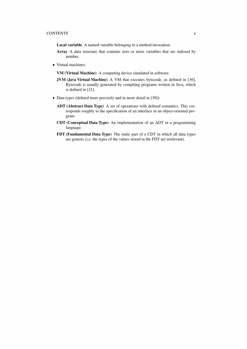
Local variable A named variable belonging to a method invocation.
Array A data structure that contains zero or more variables that are indexed bynumber.
• Virtual machines:
VM (Virtual Machine) A computing device simulated in software.
JVM (Java Virtual Machine) A VM that executes bytecode, as defined in [36].Bytecode is usually generated by compiling programs written in Java, whichis defined in [21].
• Data types (defined more precisely and in more detail in [30]):
ADT (Abstract Data Type) A set of operations with defined semantics. This cor-responds roughly to the specification of an interface in an object-oriented pro-gram.
CDT (Conceptual Data Type) An implementation of an ADT in a programminglanguage.
FDT (Fundamental Data Type) The static part of a CDT in which all data typesare generic (i.e. the types of the values stored in the FDT are irrelevant).

Chapter 1
Introduction
As software has grown more complex, the amount of errors in it, known as bugs, has in-creased. Market pressures can further compound this problem by causing a project to bedeveloped with unskilled programmers or insufficient time or money. It is estimated thatsoftware errors lead to costs of tens of milliards of euros every year. [49]
Bugs are essentially a difference between the intended behaviour of the program andits actual behaviour. Thus, one way to find and eliminate bugs (an activity known as debug-ging) is to examine the operation of the program and compare this to the desired operation.This approach is called testing. Tools that assist in debugging by allowing programmersto examine the current state of a program (which includes the data the program is work-ing with in memory and the currently executing code) and control its execution are calleddebuggers.
Current debuggers have several limitations. As they generally show data by display-ing the values of individual variables, it is often hard to see the interesting aspects of therunning program and its data. Object-oriented development has allowed programmers tohide unnecessary detail while developing, but debuggers generally do not take advantageof this. Furthermore, it is difficult to test results of operations in the program without writ-ing additional code that runs parts of the program and examines the results. Also, when aproblem is found, its cause is often lost in the past, which necessitates careful rerunningand stepping through the program to find the cause of the problem.
In order to teach students algorithms better, many universities have developed algo-rithm animation tools that display the execution of algorithms as a sequence of graphicalrepresentations of a data structure. Algorithm animation can also be used in conjunctionwith user-controlled algorithm simulation. Algorithm simulation allows students to exam-ine the behaviour of algorithms by specifying the operations to perform and watching theresults. Usually, the algorithm simulation tool provides a graphical user interface (GUI)that shows the data structures and allows the user to perform operations on them (such asadding or modifying data) using common GUI input techniques such as clicking or drag-ging and dropping.
Algorithm animation and simulation tools provide a way of visualising data structuresthat makes the relevant data easier to find and comprehend and a simple mechanism forcontrolling operations on these data structures. User-controlled algorithm simulation is con-ceptually quite similar to testing, which suggests that some techniques used in algorithmsimulation can be applied to testing.
1.1 GoalIt seems that an unfulfilled need for a better way to examine and test software exists. Specif-ically, something is needed to aid in the following tasks:
1

CHAPTER 1. INTRODUCTION 2
• Testing code to see if it works and identifying the faults if it doesn’t.
• Studying code to understand what it does and how it works.
1.2 Proposed solutionThe solution presented here to the problem of testing and examining programs is visual test-ing, in which the visualisation and control techniques of algorithm simulation are appliedto the problem of testing software. The programmer using visual testing should be ableto examine the operation of a program visually without being bogged down with imple-mentation details. He should also be able to choose which parts of the program to executeand manipulate the data to be processed by the executing program. The visual testing toolshould interact with its users through a graphical user interface.
1.3 Thesis outlineThe following issues are addressed in this thesis:
• The desired properties of a visual testing tool (Chapter 2).
• A survey and evaluation of debugging and software visualisation tools that can beused for visual testing (Chapter 3).
• Descriptions and evaluations of visualisation (Chapter 4), elision and abstraction(Chapter 5) and control techniques (Chapter 6) suitable for visual testing.
• Different approaches to the implementation of a visual testing tool (Chapter 7).
• The design of a fully fledged visual testing tool (in Chapter 8).
• The design and implementation of a prototype visual testing tool that demonstratesthe feasibility of the visual testing concept and the new techniques applied in it (inChapters 8 and 9).
• Some use cases that can be used to demonstrate and evaluate the prototype visualtesting tool (Chapter 10).
• An evaluation of the prototype (Chapter 11).
• Conclusions and suggestions for future studies (Chapter 12).

Chapter 2
Objectives
The goal of a visual testing tool is to provide programmers with the ability to examine whattheir program does interactively, by allowing monitoring and manipulation of program ex-ecution and data. This allows the programmer to try out the results of manipulating objectsand executing methods.
2.1 CriteriaThe goal of a visual testing tool can be split into the following criteria:
Generality The testing tool should work on programs not specifically designed or writtenfor visualisation; in other words, the user should not need to change his programsto use the tool with them. Ideally, any program can be examined. This criterion cor-responds to requiring generality and scalability (both parts of scope) as defined byPrice et al. in their taxonomy of software visualisation [46]. Lack of generality usu-ally means that programs must be rewritten to fit the tool. However, dissimilar pro-gramming languages require different visualisation strategies, so it is unrealistic andnot very useful to be able to use the same tool on programs written in completelydifferent languages.
Completeness All aspects of the running program should be accessible for examination.In most object-oriented languages this encompasses:
• An execution stack or call stack for each execution thread, which typically con-tains information on the currently active method invocations and their localvariables.
• All objects and variables.
• Code and current execution position.
This corresponds to fidelity and completeness in the Price et al. taxonomy.
Data modification Variable values should be freely modifiable where allowed by the pro-gramming language. Software visualisation does not usually address this aspect, al-though it is common in debuggers.
Execution control The user should be able to try out any part of the program on data ofhis choice and execute operations of his choice on the data in the running program.Ideally, the user should be able to control what is executed down to individual op-erations and create and modify classes and methods on the fly. Being able to invokemethods at will is the most important part of execution control. Control of this typeis a fundamental part of algorithm simulation.
3

CHAPTER 2. OBJECTIVES 4
Presentation Ideally, the testing tool would automatically present exactly what the userwants to know about the program, its execution and its data in the form in which hethinks about these matters. The data should be represented in such a way that the usercan easily find the information he requires, and the information is expressed clearly.Visual representation is clearly the most effective way of conveying this informationin practice, although visual information can be augmented with sound or informationfor any other sense. Finding a visual representation that meets these requirementsis one of the main problems in constructing a visual testing tool. In practice, thisincludes:
Representation The data must be shown in a suitable (graphical) form.
Abstraction Unnecessary implementation details should be abstracted away when-ever it is possible and the user desires it. Implementation details that were hid-den from the user during programming that he does not care about should alsobe hidden while debugging (one aspect of appropriateness and clarity in Priceet al.).
Automatic view control The tool should guess at what the user wishes to see andpresent the data in this form (another aspect of appropriateness and clarity inPrice et al.).
Manual view control The user should be able to change the view easily to matchhis own ideas by hiding (eliding) parts of the view and changing the way inwhich information is represented (navigation in Price et al.).
The mapping between the data in the running program and the visualisation shouldwork both ways; if the user modifies data in the graphical view, the correspondingchange should be made to the data in the debuggee.
Causal understanding It should be easy to understand the reason for the current stateof the program. Ideally, we could ask the computer something like “Why is thisreference null?”, and it would answer, for example, “Because you put these twostatements in the wrong order.”. In order to do this, the computer would have tounderstand what was expected of it and be able to write correct code, which woulddefeat the purpose of having an interactive testing tool. Therefore, a more realisticgoal must be set.
A more realistic goal is that the user should be able to examine the entire executionhistory of the program (or at least selected interesting parts of it) and search throughit for the instructions, instruction sequences or events that caused a specified changeto the state of the program or caused it to differ from the expected state. This is theapproach taken by algorithm animation.
2.2 ScopeDesigning and writing a visual testing tool that provides all features that could possibly beuseful for the testing, debugging or examination of any program written in any language isa very large undertaking. Therefore, the scope of this thesis must be a carefully boundedsmall subset of the area of visual testing.
2.2.1 Target languageObject-oriented languages are especially well suited to working at high abstraction levels,as they provide many mechanisms for encapsulation and abstraction. Many languages thatare in heavy use today are object-oriented, such as Java and C++. Because of these twofactors, this thesis will focus on object-oriented languages.
CHAPTER 2. OBJECTIVES 5
The prototype is designed to process programs written in Java (described in [21]), be-cause:
• Java is highly portable, as Java software can be run on any platform with a JVM.This makes the results more widely applicable.
• Java is object-oriented, which encourages programmers to write code at a higherabstraction level and with more modularity than in e.g. C. This makes it easier toconstruct visualisations of a program similar to the concepts in a programmer’s mind.
• Java is widely used:
– A lot of software has been written in Java.
– Java is often used to teach programming.
– Programmers with Java skills are highly sought after [76, 79].
This means that a wide range of software is available and being written in Java thatcan be used with the results of this work.
• Java is considerably less complex than C++. This simplifies the design a lot.
In matters that are not specific to Java, generalisation to other similar languages is alsodiscussed here.
2.2.2 Solution types to considerThe solutions to the problems posed in the introduction will be based on techniques fromexisting debugging, software visualisation and algorithm animation and simulation soft-ware, whenever these techniques can be adapted to suit visual testing.
Techniques that seem to provide little extra comprehensibility but require a lot of extrawork, such as smooth animation, sound or three-dimensional visualisation, will also be leftout of consideration. This work will concentrate on ways to visualise the data structuresand execution flow of a running program using two-dimensional graphics and interact withthe running program.
2.2.3 PrototypeIn order to examine how well visual testing works in practice, a working implementationshould be made. However, features that are not essential to visual testing can be left out,especially if other software already provides similar functionality. This prototype shouldallow examination of programs written in Java. If possible, existing software (debuggers,visualisers or similar tools) will be used as a basis for the prototype.

Chapter 3
Related work
Software visualisation can be divided into three categories based on the purpose of thevisualisation and the approaches used:
• Visual debugging.
• Program visualisation.
• Algorithm animation and simulation.
The program visualisation and debugging approaches are based on the idea of taking a run-ning program, stepping through it and showing the variables and other interesting parts ofthe state of the executing program. This shows what the program is doing. Program visu-alisation is used to understand a program, while debugging involves finding and correctingerrors in a program. Program visualisation and debugging can be done using similar tech-niques and in some cases both may be combined in a single tool (e.g. Lens [37, 38] andLeonardo [23]).
The algorithm animation approach is based on showing a series of graphical represen-tations of a data structure at successive points in time in order to explain how an algorithmoperates on the data structure. Many algorithm animation systems allow the user to stepback and forth through the states of the data structure and algorithm to study the progressof the algorithm. User-controlled algorithm simulation gives the user the ability to manip-ulate the data structures himself.
In this chapter, debugging and program visualisation systems designed for procedurallanguages (with or without object-orientation) such as C, C++, Pascal and Java are sur-veyed. Debuggers and program visualisers for other languages are only included if theyhave features or properties that may be of use in visual testing; visualising the executionand data structures of programs written in e.g. Prolog or Lisp is an entirely different prob-lem due to the different execution and data models used in these languages. Also, the mostimportant general-purpose algorithm animation and simulation tools are described.
3.1 DebuggingDebuggers are intended to be used to find bugs in programs by tracing through the exe-cution of program and examining and editing variable values. Most debuggers have someexecution control facilities (e.g. single step, breakpoints, watchpoints and expression eval-uation) and some way to view variable values.
Most debuggers are based on ideas from FLIT (Flexowriter Interrogation Tape), whichintroduced symbolic debugging (meaning that the user could work with variable names,labels and instruction mnemonics instead of memory addresses and numerical instructioncodes) and breakpoints [55]. More than 40 years later, most current debuggers are based
6
CHAPTER 3. RELATED WORK 7
on the same paradigm: run the program to a specified point, stop it and examine the valuesof the variables. A few improvements have been made, such as single stepping. Thesedebuggers can be referred to as command line debuggers (referring to their user interface)or traditional debuggers (referring to their heritage).
The most common style of debugger today is a traditional debugger with a graphicaluser interface. Most integrated development environments (development software packagescontaining an editor, a compiler and linker and a debugger within a common user interface),such as Borland JBuilder and Microsoft Visual Studio, contain a debugger of this type [72,80]. Debuggers of this type are referred to by their authors as “visual debuggers” (e.g.the Javix Visual Debugger [68] or the Tango/04 VISUAL Debugger [78]) or “graphicaldebuggers” (e.g. KDbg [75] or JSwat [66]). To avoid confusion, I will refer to debuggersof this type as graphical debuggers. These debuggers have few interesting features from avisual testing viewpoint and are too numerous to survey properly. For these reasons, theyare not included here unless they have other features that merit attention.
During the last two decades, visualisation features have been developed for debuggingtools. Two approaches to visualisation in debuggers can be discerned. The simpler ap-proach is to allow the user to select concrete data structures to be displayed and displaythe primitive values in them and references between them without any attempt to interpretthe meaning of the data. This approach is used by most debuggers intended for develop-ment use (e.g. DDD [63] and GVD [67]) and those intended for novice programmers (e.g.Amethyst [39]). The other approach allows the user to create visualisations for his programby constructing animations using predefined primitives and the variables in the program.This allows the user to view his data at a higher level of abstraction, but also requires morework to get the desired view. This approach is also sometimes used in program visualisa-tion, which makes it hard to classify some of the programs that use it (e.g. Lens [37, 38]).Debuggers that use software visualisation techniques are generally called visual debuggersalthough they are also sometimes confusingly referred to as “graphical debuggers”.
BlueJ [27] is not quite a debugger; it is primarily a development and testing tool, al-though it also has debugging features. It is included here because of its interesting approachto testing.
In the following, each surveyed debugger is briefly presented.
3.1.1 DDDDDD (Data Display Debugger) [62, 63] is a visual debugger that provides extensive de-bugging facilities and some (low-level) data structure visualisation, mostly limited to dis-playing structs or classes as boxes with pointers shown as arrows between them, as well asplotting array data using the plotting program gnuplot. DDD makes use of a command linedebugger, such as GDB or JDB, to debug programs written in a variety of languages, suchas C, C++, Java, Pascal, FORTRAN, Python and Perl.
GVD (GNU Visual Debugger) [67] has a similar feature set and user interface.
3.1.2 RetroVueRetroVue [14, 81] by VisiComp allows the user to browse the execution history of an exe-cuting Java program by watching it execute (either in real time or from a log), by steppingbackwards or forwards through the logged states or by searching for specific events. Thestate of the program is shown using the following views:
• A thread view that shows the state of the different threads (running, runnable, blocked,et.c.) as a function of elapsed time. Locking and deadlocks are clearly indicated.
• The execution history of the program (as a tree structure of nested method calls andstatements).
CHAPTER 3. RELATED WORK 8
• A tree view of the static structure of the program (classes, fields, methods, et.c.).
• A tree-structured data view based on showing the local variables and expandingbranches representing references to other objects.
RetroVue is thus essentially a graphical debugger with the ability to step back and forththrough the execution history of a program or examine the history as a tree.
3.1.3 ODBLike RetroVue, ODB (the “Omniscient Debugger”) [35] collects information about theoperations performed by an executing Java program and allows the programmer to exam-ine the execution history. Like RetroVue, ODB supports stepping backwards and forwardsthrough the execution history. Unlike RetroVue, ODB allows the user to interrupt the run-ning program and execute methods and modify data values in a secondary timeline thatstarts from a copy of a state of the real execution history. The main timeline containing thereal execution of the program may not be modified.
ODB shows the threads in the program, their stack, the tree of executed methods and atreelike view of selected objects and objects they refer to.
3.1.4 AmethystThe Amethyst visual debugger [39] displays call stacks, variables, arrays and records graph-ically for a running Pascal program. Records and arrays are displayed as nested boxes. Heapobjects and pointers are not supported. Amethyst also provides graphical control over step-ping and breakpoints.
3.1.5 LensThe Lens visual debugger [37, 38] is an attempt to bridge the gap between program vi-sualisation and algorithm animation. It is based on the XTango animation system and thedbx command line debugger, and allows the construction of animations based on data inprograms. The user constructs an animation by creating graphical objects (lines, rectan-gles, text and object arrays, for instance) and adding animation commands that affect theseobjects to the source code, such as “move”, “colour” or “delete”. The actions are definedusing a graphical editor. Lens has some limited execution control facilities and allows theuser to access the underlying debugger directly.
Getting a high-level visualisation out of Lens requires quite a lot of extra work, as youessentially have to design the visualisation yourself. The additional programming requiredto produce a visualisation discourages programmers from using Lens. [24]
3.1.6 BlueJBlueJ [27] is an integrated development environment for Java designed for use in intro-ductory programming courses. BlueJ displays the structure of a Java program in a fashionsimilar to a UML class diagram, and allows the user to graphically instantiate objects andexecute methods. BlueJ allows the user to inspect values of variables, but it does not pro-vide any data visualisation beyond a simple graphical debugger, which supports stepping,breakpoints and can shows lists of local variables, fields of an object or class and currentlyactive methods.

CHAPTER 3. RELATED WORK 9
3.2 Program visualisationThe purpose of program visualisation is primarily educational. The goal is usually to helpthe user understand or explain to others how a program works. Most of these systems aretargetted at teaching basic programming (especially Eliot [58], its successor Jeliot [22] andthe system designed by Korsh, LaFollette and Sangwan [32, 33, 50]), while others are (also)intended to help programmers understand what a program is doing (e.g. VisiVue [81] andProsasim [73]).
While debuggers are traditionally based on stopping program execution and examiningthe state of the program, program visualisation systems use a greater variety of approachesto extracting information from a running program. Some require that the user add visuali-sation commands to their program (e.g. Leonardo [16]), while others automatically add vi-sualisation code to the user’s program using a modified compiler or additional precompiler(e.g. Eliot [58] and Jeliot [22], VCC [5] and UWPI [23]). Finally, some use debugger-styleexamination of running programs (e.g. VisiVue [81]).
While most program visualisers use a finished program (possibly with graphics callsadded) as input, Prosasim [73] is based on simulating a system described as a UML model.
Program visualisers with no features relevant to visual testing that cannot be found inother program visualisers have been left out. These include the system described by Rasalain [47]. Systems that only visualise source code or other static structures, such as Source-Navigator [77] are not included here.
3.2.1 JeliotThe Eliot [58] and Jeliot [22] program visualisers display the data structures of an executingprogram (at quite a low level; primitives, arrays, stacks and queues) with smooth animationby instrumenting the code on compilation. Jeliot is used as a client/server program overthe web; the client supplies source code in EJava (a modified version of Java with addedstack and queue types and some limitations), which the server precompiles to Java (addinganimation code in the process) and compiles into an animation applet. Eliot uses C andC++ instead of Java and is not designed for use over WWW. Eliot also works with low-level built-in data types such as integers, arrays and trees.
3.2.2 VCCThe VCC [5] system adds animation features to C programs using a modified compiler thatadds animation code. VCC shows the currently active function (with arguments and localvariables), the tree of executed program calls, the program code, standard I/O and separatedata views for records (structs) and arrays. However, VCC does not visualise dynamic(heap-allocated) structures.
3.2.3 UWPIThe UWPI [23] system is based on a specialised Pascal compiler that adds data visualisationthat attempts to recognise known idioms (common data structure operations) and from thisrecognise abstract data structures for visualisation such as Boolean or reference variables.
3.2.4 Korsh-LaFollette-SangwanThe system designed by Korsh, LaFollette and Sangwan [32, 33, 50] is essentially a datavisualisation and animation system for C/C++ programs based on modified data types withoverloaded operators containing animation calls. It displays the code, heap, call stack, localvariables, arguments and operations being performed. The system is intended for use inbasic programming courses and therefore only handles integers, structs and pointers.

CHAPTER 3. RELATED WORK 10
3.2.5 ProsasimProsasim [73] takes an executable UML model of a program built using the Prosa modellerand simulates its execution. The model can then be visualised using the UML diagrams(e.g. collaboration diagrams) in the model. The values of attributes in the model can alsobe examined. Using the Prosaj or Prosacpp code generators, this model can be convertedinto an executable model in Java, C or C++.
3.2.6 LeonardoThe Leonardo [16] software visualisation environment allows the user to edit, compile,execute and animate C programs. It uses a virtual processor to provide debugging facili-ties including reverse execution. Graphical interpretations are specified using declararationswritten in the logic programming language Alpha embedded in the C program as comments.Using Alpha, the programmer can construct many types of visualisations containing geo-metric primitives or graphs. However, Leonardo is hard to classify, as it combines aspectsof emulation, debugging and program visualisation.
3.2.7 VisiVueVisiVue [81] by VisiComp visualises and animates objects in an executing Java program.The animation is done while the program executes, with highlighting to indicate the cur-rently executing statement. It also produces textual execution trace logs.
3.2.8 PavanePavane [48] visualises the state of a program written in Swarm, consisting of a set of tran-sition rules and a defined initial state to which the rules are applied. Pavane uses declarativevisualisation; a mapping between the program and a world of 3D geometric objects is de-fined as a set of rules.
3.2.9 DynaLabDynaLab [9] consists of a virtual machine connected to a simple program animator thatdisplays the current execution position in the source code, the currently active proceduresand their local variables textually. The virtual machine is capable of reverse execution.Compilers for DynaLab’s virtual machine exist for Pascal, Ada, C and C++. Only the Pascalcompiler has been completed and released.
3.2.10 TarraingímTarraingím [40] visualises programs written in the object-oriented programming languageSelf. Besides displaying the actual data contents of objects, Tarraingím can display objectsgraphically at a higher level of abstraction using view code written to monitor and accessobjects through their interfaces.
3.2.11 JAVAVISJAVAVIS [43] visualises the current state of a Java program as a set of UML object diagrams(one for every active method invocation) containing the local variables of the method andall objects reachable from these local variables by following references. JAVAVIS also vi-sualises the executed method calls of a Java program as a sequence diagram.

CHAPTER 3. RELATED WORK 11
3.3 Algorithm animation and simulationMost algorithm animation and simulation tools are designed for the teaching of algorithmsand data structures. Their purpose is twofold: to make it easier for teachers to show theirstudents what an algorithm does (Balsa-II and Zeus emphasise this application [10, 11]),and to allow the student to experiment with data structures and algorithms (Matrix andJDSL emphasise this area [6, 29, 31]). Algorithm animation tools designed for students’use often automatically visualise data structures that conform to a predefined interface,while those designed for teachers’ needs usually require the user to add explicit graphicscalls.
This survey does not include graphics libraries that only provide geometric primitivesand animation, such as XTango [52] and Polka [54]. These libraries leave most of the hardwork of constructing a visualisation to the user. Animation tools that only work with ge-ometric primitives, such as ANIM [8] and Samba [53] and its derivatives, have been leftout for similar reasons. Systems superseded by newer systems by the same authors, such asBalsa [13] and WWW-TRAKLA [28], have also been left out. Algorithm animation sys-tems designed for a few specific algorithms or a small class of algorithms (e.g. geometricalgorithms) have been left out of consideration due to their amount and limited applicabil-ity. A wide range of specialised algorithm animation tools can be found at [65].
3.3.1 MatrixThe Matrix [29, 31] system provides animation (including stepping both backwards andforwards) and user-controlled simulation of data structures written to conform to specifiedinterfaces. Unlike the other systems described here, Matrix allows hierarchical compositionof types. Matrix supersedes the old Trakla system, which was limited to user-controlledsimulation of a few built-in data structures.
3.3.2 JDSLThe JDSL Visualizer [6] provides animation and visualisation of data structures written toconform to specified interfaces (those of the JDSL data structure library). By default, itshows the data structure before and after API calls, but additional animation frames can begenerated by adding calls to the visualiser. The JDSL Visualizer allows the user to selectmethods and their arguments and execute the methods (as defined by the user) on the datastructures. JDSL shows the history of events that have happened to the data structure andthe current state of the data structure.
3.3.3 Balsa-IIThe Balsa-II [10] system is an algorithm animation tool. It animates algorithms written inPascal with explicitly added display calls and conforming to a specified interface. The al-gorithm outputs change events through an adapter to a modeller, which maintains a genericdata model that can be used by several viewers, which display the data in the model.
3.3.4 ZeusThe Zeus [11] algorithm animation system is similar to the authors’ previous system, Balsa-II, but adds support for allowing the user to generate events with specified arguments (sim-ilar to calling methods). Zeus works with Modula-2 code.
CHAPTER 3. RELATED WORK 12
3.3.5 AlgAEAlgAE [61] animates algorithms that are implemented in Java or C++ conforming to thevisualiser’s interfaces. The algorithms must be annotated with explicit visualiser calls. Al-gAE also provides a graphical user interface with which the user can invoke algorithms ona data structure. The visualisation consists of boxes that can contain text, other boxes andlinks or arrows to other objects. AlgAE does not appear to support moving back and forththrough the execution of the algorithm.
3.3.6 World-wide algorithm animationThe World-wide algorithm animation [25] system (hereinafter WWAA) is designed to al-low students to manipulate (through a web browser) algorithm implementations writtenin Pascal (with lots of calls to the animation system) running on a server. WWAA allowsusers to step through an algorithm implementation or run it to the end or a breakpoint andview and modify variable values. It can also forward bitmap images containing graphicalrepresentations of data structures.
3.3.7 JAWAAJAWAA [44] executes animation scripts generated by a program to which animation outputcommands have been manually added. The animation can include primitive graphical ob-jects such as lines, text and rectangles as well as arrays, stacks, queues, graphs and trees.Once the animation script has been created, the user can run or step forward through theanimations.
3.3.8 JCATJCAT [12] animates algorithms written in Java annotated with visualiser calls. The visu-aliser calls are passed to a view applet designed for a specific data structure or algorithm.The view applet uses an animation package based on a graph containing vertices that canbe connected with edges and moved to different positions smoothly. The vertices can havevarious graphical properties such as a textual label, a polygonal outline or colour.
3.3.9 JIVEJIVE [70] animates algorithms written in Java using a set of pre-written data structures withanimation hooks. The data structures supported by JIVE include graphs, binary trees, listsand hash tables. The algorithm can request user input, such as selecting a graph vertex orentering a number. JIVE also allows the user to manipulate the data structures graphically.
3.4 EvaluationI have evaluated tools for suitability for visual testing by checking how well they meetthe criteria mentioned in this section. The evaluation results use the notation defined inTable 3.1.
In order to evaluate the previously done work in this area, I compare the systems againstthe requirements listed in section 2.1. The results of this comparison are shown in Table 3.2.
3.5 AnalysisThis section summarises the survey results and describes some commonalities in the sur-veyed tools.

CHAPTER 3. RELATED WORK 13
Score Meaning- The system does not meet the criterion at all; the system has no func-
tionality of this type.p The system meets the criterion partially; the system has some limited
functionality of this type that may be occasionally useful.pp The system meets the criterion well enough for basic use; the system
provides functionality of this type that is usually sufficient.ppp The system meets the criterion very well; the system provides excellent
functionality of this type that handles even complex cases well.
Table 3.1: Scoring system for evaluation of tools
System Gen
eral
ity
Com
plet
enes
s
Dat
am
odifi
catio
n
Exe
cutio
nco
ntro
l
Rep
rese
ntat
ion
Abs
trac
tion
Aut
omat
icvi
ewco
ntro
l
Man
ualv
iew
cont
rol
Cau
salu
nder
stan
ding
DDD ppp ppp pp pp pp - p pp p
RetroVue ppp ppp - p p - - pp ppp
ODB ppp ppp pp p p p - pp ppp
Amethyst pp p p pp pp - p - -Lens ppp ppp p p pp pp - pp p
BlueJ ppp ppp p ppp p p - pp -Jeliot pp p - p pp p - pp -VCC ppp p - p pp p pp p p
UWPI p p - - pp pp pp - -Korsh et al. pp p - p pp pp pp - -Prosasim p pp ppp ppp ppp p pp pp p
Leonardo pp pp - p ppp ppp - pp pp
VisiVue ppp p - p pp - pp p -Pavane p pp - p ppp ppp - ppp -DynaLab pp pp - pp p - pp - pp
Tarraingím p pp p p ppp ppp pp ppp -JAVAVIS ppp pp - p pp - pp p -Matrix p p pp pp ppp pp pp pp pp
JDSL p p pp pp pp pp pp - pp
Balsa-II p p - p pp pp pp pp p
Zeus p p - pp pp pp pp pp p
AlgAE p p - pp pp pp - pp -WWAA p p pp pp pp pp - pp -JAWAA pp pp - p pp pp - ppp -JCAT pp pp p pp pp pp - ppp -JIVE p p pp pp pp pp pp pp -
Table 3.2: Evaluation of previous work

CHAPTER 3. RELATED WORK 14
3.5.1 Traditional groupingThe common properties of the tools in each group and the differences between them aredescribed in this subsection.
Debugging
In general, debuggers concentrate on generality, completeness and data modification. Exe-cution control in debuggers is often limited to placing breakpoints and stepping (Retrovue,ODB and Lens), but some allow the user to invoke methods, functions or similar constructs(DDD, Amethyst, BlueJ).
RetroVue, ODB and BlueJ show data structures using techniques from (non-visual)graphical debuggers; they do not provide data structure visualisation. They are includedhere because of other interesting features; RetroVue and ODB are designed to addressthe problem of causal understanding, while BlueJ provides a new form of object-orientedexecution control. In contrast, DDD, Lens and Amethyst all provide simple low-level visu-alisations.
Program visualisation
Program visualisation tools generally concentrate on presentation, although some (e.g.Leonardo) handle most of the other aspects as well. Most of these systems place muchof the burden of extracting relevant information on the user (for example, Leonardo of-ten requires extensive visualisation declarations to produce visualisations, even though theoriginal code can be left mostly unmodified), while others ignore this problem entirely anddisplay data structures at a very low level (e.g. Jeliot). Some program visualisers concen-trate on displaying only specific types of data stored in variables (e.g. Jeliot, UWPI) oronly objects (VisiVue). VCC and the system by Korsh et al. limit their support for prim-itives to integers, but support arrays, structs and pointers. Program visualisers often placemore constraints on the program to visualise than debuggers, such as requiring programs tobe written in modified versions of a common programming language (Jeliot, VCC, Korshet al.), for a limited environment (Leonardo), in a limited subset of a language (UWPI)or in a specialised language (e.g. Pavane). In short, program visualisation tools usuallyconcentrate on visualising a particular aspect of a program, and usually require more userintervention to produce a visualisation than a visual debugger.
Prosasim is a bit of an odd man out, as it relies heavily on programs being writtenusing the Prosa modeller. However, this means that the program can be both written anddebugged using the same representations and metaphors.
Algorithm animation
Algorithm animation systems generally concentrate on presentation, abstraction and/orcausal understanding. User-controlled algorithm simulation adds extensive execution con-trol and data modification abilities to this.
The algorithm animation systems mentioned here can be used to visualise data struc-tures in user programs, but extensive writing of code to map the data to the data typessupported by the system is usually necessary. Matrix has greater expressiveness in its datastructure representations than the other algorithm animation systems thanks to its ability toform nested structures inside other structures. When using most of the algorithm animationtools, the user must extensively modify his program to conform to an interface that can bevisualised.
Some algoritm animation tools (e.g. Matrix and JDSL) also support algorithm simula-tion, which allows data structures to be modified according to data structure-specific rules.

CHAPTER 3. RELATED WORK 15
3.5.2 Grouping by data extraction approach and code preprocessingFrom the point of view of visual testing, the difference between algorithm animation, pro-gram visualisation and visual debugging is quite small. One of the most important questionsis “How much do I have to modify or annotate my program to visualise it?”. The generalityvalue shown in Table 3.2 reflects this, as the amount of changes that must be made to aprogram depends on the requirements placed by the visualisation system on the program.The requirements in turn depend on the approaches used to define the visualisation andmonitor the state of the program.
The surveyed visual debuggers (with the exception of Amethyst, which only supports asubset of Pascal) can visualise every important aspect of practically any program written inat least one common programming language and therefore have very good (ppp) generalityand completeness. The visual debuggers based on taking snapshots of data at breakpoints(DDD, Amethyst, BlueJ and Lens) have very limited support for examining the executionhistory of a program, which implies limited (- or p) causal understanding. However, debug-gers based on automatic instrumentation of Java bytecode (RetroVue and ODB) can recordthe execution history of a program and allow the user to examine it in many ways, which isvery good (ppp) for causal understanding.
Most algorithm animation and simulation tools require that a program be written toconform to their data structure or algorithm interfaces or use their predefined data struc-tures. Rewriting a large program to conform to these interfaces can be laborious and mayresult in even more bugs to track down, especially if the data structures used by the visual-isation differ significantly from those in the program to be visualised. Similarly, no aspectsof the program’s function other than those explictly defined in the predefined data struc-tures or interfaces are visualised. These systems therefore have only limited (p) generalityand completeness. JCAT and JAWAA only require visualisation calls or output commandsto be added, which removes the need for restructuring and allows information that is notstored in a suitable data structure to be visualised. This increases the generality and com-pleteness to a sufficient level for basic use (pp). All of these data collection techniques allowlogging of execution history, but only a few of the systems actually implement this (Matrixand JDSL have a general logging facility, while Balsa-II and Zeus can provide specialisedhistory views in some cases).
The program visualisers have the greatest variety of approaches to defining the visuali-sation and monitoring the program. VCC, VisiVue and JAVAVIS require almost no manualintervention to visualise almost any program written in the right language and thereforehave very high (ppp) generality. UWPI only supports a small subset of Pascal, which limits(p) its generality. Jeliot does not require manual modifications, but it can only visualise sim-ple programs without modifications due to implementation limitations, which decreases itsgenerality somewhat (pp). Leonardo and DynaLab use virtual machines and special compil-ers that lack some commonly used features that are available in many of the environmentsfor which software is written, such as networking, which decreases their generality ratingsimilarly (pp). Tarraingím, Pavane and Prosasim rely on special features of unusual pro-gramming languages, meaning that most programs will have to be rewritten completely tobe used with these tools, which means that they have very little generality (p). The system byKorsh et al. relies on using specialised data types, like most algorithm animation systems.However, replacing standard C/C++ data structures with those used by the Korsh systemis reasonably straightforward, which means that it has sufficient (pp) generality. Most of theprogram visualisers concentrate on particular aspects of a program (which severely limits(p) their completeness), but some provide almost complete views of most of the interestingaspects of the program’s state (sufficient (pp) completeness).
In other words, grouping the surveyed systems by the data extraction approach and codepreprocessing techniques used produces the division in Table 3.3. The scores shown in thetable are the highest in each category, as this reflects the potential of the approach.
Based on this, automatic instrumentation appears to be the most suitable approach for

CHAPTER 3. RELATED WORK 16
Type of system Gen
eral
ity
Com
plet
enes
s
Cau
salu
nder
stan
ding
SystemsSnapshots taken at breakpoints ppp ppp p DDD, Amethyst, BlueJ, LensAutomatic instrumentation ppp ppp ppp RetroVue, ODB, VCC, VisiVue,
JAVAVIS, Jeliot, UWPIPredefined data structures or inter-faces
pp p pp Matrix, JDSL, Balsa-II, Zeus, Al-gAE, WWAA, JIVE, Korsh
Annotation without restructuring pp pp p Balsa-II, Zeus, JCAT, JAWAASpecialised execution environments pp pp pp Tarraingím, Pavane, Prosasim,
Leonardo, DynaLab
Table 3.3: Surveyed systems grouped by data extraction approach
visual testing.
3.5.3 Grouping by view control styleTwo of the other most important questions when evaluating suitability for visual testingare “How much does the representation look like what I want?” and “How much of thework in producing the visualisation is done automatically?”. In Table 3.2, the first of thesequestions was answered by the representation, abstraction and manual view control ratings,while the second is answered by the automatic view control rating.
All of the debuggers (except Lens and Amethyst) and some program visualisers (JAVAVIS,DynaLab and VisiVue, Jeliot) display objects and similar data structures only if the userexplictly asks to see them as a set of fields or with minimal abstraction of implementationdetails. This provides sufficiently good (pp) manual view control, but automatic view controlthat is limited at best (- or p) and a limited degree of abstraction at best (- or p). The view canconsist of an object graph (which is usually a sufficiently good (pp) representation) or textualfield displays (which is not a clear representation in the general case (p)). Amethyst is sim-ilar, but it displays all variables in the current procedure or function (limited (p) automaticview control and no (-) manual view control). VCC provides acceptable (pp) automatic viewcontrol, but is otherwise similar to this group.
The system by Korsh et al. and UWPI attempt to deduce the right abstractions andrepresentations themselves, giving them good enough (pp) support for abstraction, represen-tation and automatic view control but no (-) manual view control.
The algorithm animation and simulation and program visualisation systems that arebased on predefined data structures or interfaces that describe data structures can usuallyproduce views that are suitable for the data structures (good or very good (pp or ppp) represen-tation and good enough (pp) abstraction and automatic view control). These include Matrix,JDSL, Balsa-II, Zeus, JIVE, Tarraingím and Prosasim.
Some systems require the user to explicitly define almost every aspect of the visualisa-tion including the position of every object in the visualisation. These are JCAT, JAWAA,WWAA, AlgAE, Jeliot, Leonardo, Pavane and Lens. They have no automatic view control,but good or very good (pp or ppp) abstraction, manual view control and representation. Tar-raingím provides this ability, but also works with data structures through their interfaces.
Grouping the surveyed systems by the data extraction approach and code preprocess-

CHAPTER 3. RELATED WORK 17
Type of system Abs
trac
tion
Rep
rese
ntat
ion
Aut
omat
icvi
ewco
ntro
l
Man
ualv
iew
cont
rol
SystemsLow-level visualisation with man-ual control
p pp pp pp DDD, RetroVue, ODB, BlueJ, Vi-siVue, DynaLab, JavaVIS, VCC
Low-level visualisation with nocontrol
- pp p - Amethyst
Data structure-based visualisation pp ppp pp pp Matrix, JDSL, Balsa-II, Zeus,JIVE, Prosasim, Tarraingím
Manual view definition ppp ppp - ppp JCAT, JAWAA, WWAA, Al-gAE, Jeliot, Leonardo, Pavane,Tarraingím, Lens
Abstraction deduced by system pp pp pp - Korsh, UWPI
Table 3.4: Surveyed systems grouped by view control style
ing techniques used produces the division in Table 3.4. The scores shown in the table areagain the highest in each category (Tarraingím has not been included in the automatic viewcontrol rating for manual view definition systems, as it scores highly in this category dueto its use of data structure interfaces).
Clearly, basing the visualisation on specified data structures interfaces is the most suit-able approach for visual testing, although adding some manual view control and automati-cally deduced abstractions may prove useful.
3.5.4 ConclusionsBased on the fact that each of the requirements for a visual testing tool is met by at leastone of the existing systems, it seems profitable to try to combine aspects of all of thesesystems to produce a more useful tool.
In particular, combining the convenience of automatic instrumentation with a visual-isation based on data structures, including automatic abstraction and some manual viewcontrol, could result in a system that is a lot more suitable for visual testing than any of thesurveyed systems.

Chapter 4
Visualisation
This chapter examines possible approaches to various aspects of visualising a running pro-gram. The design choices made in visualisation directly affect completeness, representationand causal understanding. They may also indirectly affect manual and automatic view con-trol.
For completeness, some sort of visualisation must be provided for every type of data andcode. Completeness in this case can be seen as providing at least satisfactory visualisationfor every type of data and code.
I have evaluated the visualisations described in this chapter for suitability for visualtesting by checking how well they meet the criteria mentioned in this section for differenttypes of information. The evaluation results use the notation defined in Table 4.1.
4.1 Primitive value representationsProgramming languages usually contain a few primitive data types. Typically, these includeseveral forms of real numbers and integers as well as characters and strings. This sectiondescribes some ways of displaying them.
4.1.1 Textual representationIn most cases, the best and most common way to represent a primitive value is as a characterstring. For example, integers have several well-known character string forms. The mostcommon form by far is a version of the Arabic numeral system which has been in use forover a thousand years with only minor cosmetic changes [42]. This notation has later beengeneralised to real and complex numbers. Moreover, characters and character strings can
Score Meaning- The visualisation does not visualise this type of information at all.p The visualisation meets the criterion partially; the visualisation can be
used, but it is quite unpractical (representation); the visualisation showsa small part of the information (completeness).
pp The visualisation meets the criterion well enough for basic use; the vi-sualisation is reasonably clear in most cases (representation); the visu-alisation shows most of the information (completeness).
ppp The system meets the criterion very well; the visualisation is very clear(representation); the visualisation shows all the information (complete-ness).
Table 4.1: Scoring system for evaluation of visualisations
18

CHAPTER 4. VISUALISATION 19
Figure 4.1: Examples of graphical representations of the real value 0.75 (from left to right:bar, circle segment, arrow position on scale, luminance)
Technique RepresentationPrimitives
Textual primitives ppp
Graphical primitives p
Table 4.2: Primitive representations
obviously be represented as character strings. The string representation for most primitivedata types is quite compact, making textual representation a good choice for visualisationof single primitives.
4.1.2 Graphical representationsAlternative graphical representations are available for primitive types, but they are oftenspecialised. For example, a real number that is known to be limited to a specified rangecan be expressed as a suitably sized bar. As most of these representations require thatadditional limits be placed on the values, they are unpractical for automatically generatedvisualisations. Program visualisation tools that require the user to define a visualisationin terms of graphical primitives (e.g. Leonardo [16]) usually support this technique. Mostgraphical representations of numbers are based on showing a part of a graphical objectsuch as a bar or circle proportional to the value to be displayed or positioning or sizing anobject according to the value. Colour can also be used; the simplest mapping from valueto colour is to make the luminance proportional to the value (e.g. 0 = black, 1 = white).It is quite hard to determine a value accurately from a colour. This representation is onlysuited for detecting large errors in values. Figure 4.1 contains some examples of graphicalrepresentations of the real value 0.75 (assuming a minimum value of 0 and a maximum of1). Characters and strings are, however, very hard to represent in a meaningful visual wayas anything else than text.
4.1.3 EvaluationPrimitives can easily and clearly be shown as text, while most graphical representationshave limited use at best. This is summarised in Table 4.2.
4.2 Array representationsArrays have a wide range of sizes. For instance, some arrays may be short lists of objects,while others can be massive tables of numeric data. In order to handle this wide range ofpossibilities, several different visualisations are needed.

CHAPTER 4. VISUALISATION 20
1 2 3 4 5 6
1 2 3 4 5 6
0 1
0 1 2
Figure 4.2: The array {{1,2,3},{4,5,6}} as a table (with and without indices)
null1
0 0 1 2321
Hello0
World12
Figure 4.3: The array {{1,2,3},null,{Hello,World}} as a table of tables
4.2.1 Arrays as listsOne of the most straightforward ways of representing an array is by expressing it as a list ofsuccessive elements. These elements are usually separated by commas. For clarity in caseswhere nested lists may occur, lists are often enclosed in some sort of brackets (usually curlybrackets). This technique is used in most command line debuggers. For example, an arraycontaining the items 123, 456 and 789 would be expressed as {123,456,789}.
4.2.2 Arrays as tablesArrays can also be displayed as tables. This notation is especially natural for two-dimensionalarrays (by default, DDD displays 2D arrays as tables [62]), although it can be used reason-ably well with tables with more or less dimensions. With three or more dimensions, somethought must be given to how to group the dimensions intuitively. One approach (whichis used by default in e.g. Matrix) is to arrange arrays contained in a horizontally arrangedarray vertically and vice versa. Figure 4.2 contains an example of showing an array as atable.
If an integer is known to be an index into an array, it can be shown as an arrow or markernext to the corresponding array element. This technique is used in e.g. Tarraingím [40].
In many programming languages, such as Java, arrays are a type of object and multidi-mensional arrays are implemented as arrays of array references. In Java, an Object arraymay contain any objects, including null references and any array (including itself) [21]. Inthis case, the references between arrays are similar to the references between objects, andcan be visualised in a similar fashion (as described in Section 4.3). Without indices, theresult for a two-dimensional table is similar to the example in Figure 4.2. However, layingout each array contained within an array separately may result in columns or rows not lin-ing up properly. This means that indices must be shown separately for each of the arrayscontained in another array instead of using a single set of indices. However, this layout hasthe advantage of adapting better to array elements of different sizes (as shown on screen).An example is shown in Figure 4.3.
4.2.3 Arrays as plotsArrays of numeric data can be represented as plots of various types (plots are also known asgraphs; I call them plots to avoid ambiguity). For example, DDD represents one-dimensionalarrays as two-dimensional plots with the array index on one axis and the value on the other(see Figure 4.4 for an example) and two-dimensional arrays as three-dimensional plots with

CHAPTER 4. VISUALISATION 21
-80000
-60000
-40000
-20000
0
20000
40000
60000
80000
0 500 1000 1500 2000 2500
sintable
Figure 4.4: A DDD/gnuplot plot of a fixed point sine table (16 bit fraction, 2048 elements,one period)
a
0 5 10 15 20 25 30 35 40 45 50 0 5 101520253035404550
-1-0.8-0.6-0.4-0.2
00.20.40.60.8
1
Figure 4.5: A DDD/gnuplot plot of ai j = sin( iπ25 )sin( jπ
25 ) (50×50 elements)

CHAPTER 4. VISUALISATION 22
50
00 50 j
i
−1 0 1
Figure 4.6: A colour plot of ai j = sin( iπ25 )sin( jπ
25 ) (50×50 elements)
the array indices on two of the axes and the value on the third (see Figure 4.5 for an exam-ple) [62]. This technique is reasonably straightforward to implement and provides a goodgraphical representation for large arrays.
The plot drawing facilities can be generalised somewhat by allowing the user to selectwhich axes to place values and indices on.
DDD handles compound variables (structs, objects, et.c.) in plots by showing all nu-meric values contained in them [62]. This technique can be used to display arrays of objectscontaining multiple numeric fields.
4.2.4 Arrays as imagesTwo-dimensional tables of numerical values shown as colour values resemble images. Inthis case, it makes sense to draw each value as a pixel instead of a box; in other words,interpret the array data as a pixmap.
This representation makes particularly good sense in the case where the two array in-dices correspond to spatial dimensions in the context of the meaning of the data.
Images are slightly easier to comprehend than 3D plots, especially at small sizes. Colourcan be used to help distinguish different values (e.g. by using a scale that goes from blueto yellow instead of black to white). Alternatively, many numeric values can be coded intothe colour at once, although this easily becomes confusing. Small differences in values areharder to detect in an image than in a 3D plot. Figure 4.6 shows an array visualised as animage.
4.2.5 EvaluationLists are a straightforward way of expressing arrays, but tables are clearer in many cases.Plots and images can noticeably improve one’s comprehension of large numerical arrays,but they are useless for most other types of array. This evaluation is summarised in Ta-ble 4.3.

CHAPTER 4. VISUALISATION 23
Technique RepresentationPlottable arrays Other arrays
Arrays as lists pp pp
Arrays as tables pp ppp
Arrays as plots ppp -Arrays as images ppp -
Table 4.3: Array representations
Figure 4.7: Example of objects in a Java program shown using DDD
4.3 Class and object representationsDDD [62] displays objects and structs as boxes containing the fields of the struct or class.References (pointers) to other objects are shown as arrows from one box to another (op-tionally labelled with the name of the reference field). Nested structs (as in C and C++programs, for instance) are shown as nested boxes. An example data view from DDD isshown in Figure 4.7. Amethyst [39] also shows records and arrays as nested boxes. Nullpointers can be shown as short arrows leading to nowhere or to a special symbol, as theabsence of an arrow or as a special symbol or text string (e.g. “null”).
In Java, no object is stored inside another object; they are all separately allocated onthe heap. This means that the program code does not distinguish between objects that arenested within another and those that are simply referred to. Thus, another criterion must beused to decide whether an object should be shown inside the object that refers to it or as aseparate object.
4.3.1 Nesting or arrows?The nested box representation makes sense in cases where an object unambiguously be-longs to a single parent object (this corresponds roughly to composition in UML), whilethe graph representation makes more sense in the general case where an object may be re-ferred to by several other objects. Deciding which one of these to use is not trivial, althoughsome rules can be stated:
• Objects without references to other objects can always be shown nested inside theobject that refers to them. This is quite intuitive for objects that wrap primitive valuesor contain only a few primitive values, especially if the objects are immutable, inwhich case there is little need to tell the difference between two objects containingthe same data.
• Cyclic object nesting should be avoided. One way to avoid it is to use the graphrepresentation. Another is to remove references that cause cycles (references froman object to one of the objects it is contained in) during abstraction, and put in aplaceholder that identifies the referenced object. The former alternative is clearer inmost cases. The latter is a convenient work-around in cases where nesting is desirablebut causes cyclic nesting.

CHAPTER 4. VISUALISATION 24
• Objects that take up a large amount of screen space should not be nested insideanother object. Alternatively, maximum size restrictions can be imposed on objectsand propagated to their subobjects as in Amethyst [39].
It should be noted that any object in memory in a C/C++ program can be referred toby a pointer, including the fields of a struct. In fact, in most implementations, every singlebyte of data and code in the program can be pointed to, irrespective of what it contains.This means that not only do the same problems with nesting apply to C/C++ programs; theproblems are actually worse.
Ownership-based nesting
One way of determining whether objects unambiguously belong to a single object is tocalculate the ownership tree of the graph (as defined in e.g. [45]) consisting of the objectsand their references to each other. An object x owns another object y if all reference chainsfrom the root object r (the only object that can be accessed without references from otherobjects) to y pass through x. An object x is an ancestor of y in the ownership tree if and onlyif x owns y. The parent of y in the tree is then the object that owns y but does not own anyobject that owns y.
The ownership tree suggests a natural nesting hierarchy with an interesting property:
Lemma 1 An object y can only be referred to by objects that are owned by y’s parent p.Proof: p owns y but not x. Thus, a path exists from the root node to x that does not passthrough p. Let us assume x refers to y. y can therefore be reached from the root node throughx without passing through p, contradicting p’s ownership of y. Thus, x cannot refer to y. �
If we nest objects inside the object that owns them, Lemma 1 implies that referencesto y can only come from p or an object z inside p. However, z is not necessarily containeddirectly in p (i.e. p need not be z’s parent). This means that references upward in the nestinghierarchy are still possible.
Ownership-based nesting has the advantage of automatically grouping objects togetherin a reasonably meaningful way. However, it has the distinct disadvantage that changesin the references between the objects can cause the nesting hierarchy to change radically,which may render it confusing to use.
As a Java method can read static variables and its own local variables at any timeand start traversing the object graph from there, it seems reasonable that the root objectshould have references to all objects that are referred to by local and static variables. This,however, means that copying an object reference into a local variable or calling an instancemethod automatically means that the referenced object is considered to belong to the root.This leads to even more unintuitive changes in the nesting. Also, the ownership diagramdepends on the currently active thread. In conclusion, ownership-based nesting can changesuddenly in some quite common cases. It is therefore not suitable for visual testing.
Selection based on object type
Due to the problems with nesting, it seems best to default to arrows in all cases exceptobjects that cannot contain references to other objects and other types for which the nestedappearance is known to be desirable, such as arrays. It makes sense to allow the user toadapt the default settings to his own code and needs by specifying the types of object thatshould be shown as nested by default.
Manual selection
The user should also be able to override the automatic nesting choices (based, for example,on the class of the object) individually for every object. This is especially useful if an objectthat is usually shown nested is unexpectedly referred to by several different objects.

CHAPTER 4. VISUALISATION 25
children[1]
TreeNode 57 TreeNode 63
children[0]
key 123
TreeNode 123
children
key 456
children
TreeNode 63key 456
TreeNode 57
children
Figure 4.8: Example of labelled references
4.3.2 Static fieldsIn order to show the values of static fields, classes can be displayed in the same way as ob-jects. In other words, classes can be considered singleton objects, where the static methodsand fields are the methods and fields of the singleton object.
4.3.3 LabellingTo help the user identify objects and their types, each object should be labelled with itstype and a unique identifier (e.g. “instance of java.lang.String, id 1234”, or morebriefly “java.lang.String 1234”). Classes can be labelled with their name (e.g. “classjava.lang.String”). The identifier for an object should be unique at least over the ob-ject’s lifetime. There is even less potential for confusion if the identifier is unique over theprogram’s entire lifetime.
In languages with pointer arithmetic, such as C++, pointers can be used as identifiers.Practically all debuggers for C and C++ use pointers to refer to heap-allocated objects.
In cases where the identity and type of an object are uninteresting, the label can be leftout to save space. This is useful when visualising e.g. arrays (as illustrated in Figure 4.3)or strings.
4.3.4 MethodsMethods can also be shown in objects and classes for reference and to allow convenientmethod invocation. In most cases, however, displaying all available methods for every ob-ject is a waste of space. For invocation purposes, putting the methods for each object orclass in a pop-up menu that is accessible e.g. by right-clicking on the object or class isalmost as convenient as showing the methods all the time and occupies much less screenspace.
Methods can also be shown as part of the code visualisation, as described in subsec-tion 4.4.4.
4.3.5 Indicating the origin of a referenceWhen showing references as arrows, there are two different ways to indicate which field ofan object contains the reference represented by an arrow.
One is to label the arrow with the name of the field and place the start of the arrow onthe edge of the referring object, as in DDD. An example of this style is shown in Figure 4.8.I will refer to this style as labelled references.

CHAPTER 4. VISUALISATION 26
key 123
TreeNode 123
children
key 456
children
TreeNode 63key 456
TreeNode 57
children
Figure 4.9: Example of nested references
Technique RepresentationObjects
Objects without nesting pp
Objects with nesting ppp
Labelled references pp
Nested references ppp
Table 4.4: Object representations
The other is to place the start of the arrow in an area reserved for the field inside theobject (the proposed pointer notation for Amethyst). Essentially, instead of a value thefield of the object would contain a small placeholder from which an arrow extends. A nullreference can be shown e.g. as a placeholder without an arrow. An example of this style isshown in Figure 4.9. I will refer to this style as nested references.
The latter approach seems to be less prone to clutter than the former, as the field namesare shown tidily next to each other instead of appearing somewhere along the arrow. There-fore it is easier for the user to visually connect the arrow with the right field. Also, the latterapproach works much better with objects nested within each other, as it allows arrows toclearly originate from a nested object instead of adding a complex label to describe therelation.
Also, the former approach becomes confusing if one wishes to mix nested and non-nested child elements in the the same array. This problem can be circumvented by display-ing the labels of all the referenced objects inside the array (like DDD does) as shown inFigure 4.8 or showing indices for the objects that are shown nested inside the array.
In short, the nested reference view is simpler, clearer and more flexible than the labelledreference view.
4.3.6 EvaluationShowing a graph of objects without nesting is acceptable in many cases, but nesting can beused to improve clarity noticeably. Similarly, labelled references between objects are oftenacceptable, but nested references are clearer. This evaluation is summarised in Table 4.4.
4.4 Code visualisationTo make it easier for the user of a visual testing tool to understand the dynamic structures(data and execution) shown by the visual testing tool, the tool must show the link between

CHAPTER 4. VISUALISATION 27
Figure 4.10: Part of a source code file as shown in DDD
these dynamic structures and the static structures of the program as described in the sourcecode. In order to do this, the source code must also be visualised to some extent.
4.4.1 Displaying source codeThe simplest way to visualise code is to display the source code text. Most visual debuggers(e.g. DDD [62, 63] and GVD [67]) just display the source code one file at a time, withannotations to indicate breakpoints, current execution position and such. Figure 4.10 showspart of a DDD code view.
4.4.2 Full-detail graphical representations of program codeTheoretically, graphical representations (such as parse trees, described in [4], for example)can be created for any programming languages without sacrificing any expressiveness, butthese representations are not very useful in the usual case where the program has beenwritten in textual form, as the textual form is more familiar to the programmer and usuallymore compact. Therefore, I will leave this approach out of consideration.
4.4.3 Colour pixel and line views of program codeBall and Eick [7] have developed a wide range of code visualisations that show variousproperties of code as colourful figures. These representations are mostly designed to trackchanges between versions and display attributes such as code age or to provide overviewsof various statistics about the code (e.g. nesting level).
These visualisations are intended for different problems than those addressed in thisthesis, although some (e.g. viewing source code with colour highlighting and an extremelysmall font) may be useful as navigational aids.
4.4.4 Graphical hierarchies for classesAs the classes/interfaces and packages of a Java program (usually) correspond to files anddirectories in a file system (respectively), the tree browsing metaphors that are commonlyused to browse file systems can also be applied to Java programs. The tree can be extendedto the method level to allow convenient access to methods in large classes.
Practically all Java development and debugging tools use the package hierarchy (or thecorresponding directory hierarchy) to browse source code. BlueJ uses the class inheritancehierarchy instead, displaying it in a form similar to a UML class diagram [27]. Both theseviews can be generated from the source code, from the compiled class files or from theclasses loaded in the executing program.
Similar techniques can be used for C++ programs, although the correspondence be-tween files and classes is not enforced by the language. Therefore, when examining C++programs, the source code must be parsed to find classes. Also, C++ allows code outsideclasses, which complicates the issue. In this case, browsing the code using directories andfiles instead of packages and classes is easier to implement and possibly easier to use.

CHAPTER 4. VISUALISATION 28
Figure 4.11: Part of a package tree of the standard library using AnyJ
Package tree
A package tree of a Java program can be generated by scanning the class path of the pro-gram. Using the source code requires additional parsing. Using the loaded classes makes ithard to access classes that have not been loaded. Therefore, the most satisfactory approachwould be to base the tree on the contents of the directories in the class path. This will causeproblems with custom class loaders, as there is no standard way to list classes available toa class loader. However, as long as only local files are used, directory listing can be used tolook for available classes.
The package tree is used to select classes to view and edit in many IDEs. Figure 4.11shows an example (taken from the AnyJ IDE).
Nested classes and interfaces in a Java program are stored as separate class files inthe same directory as the class to which they belong [56]. Therefore, nested classes andinterfaces will be shown as classes belonging to the package in which they reside, if thepackage tree is generated from directory listings of a file system instead of the source code.
The package tree can also be extended to contain the methods in each class. Many IDEs,such as AnyJ, do this to allow easier editing and viewing of source code.
Class diagrams
UML class diagrams can also contain information on other relationships between classes,such as composition, aggregation and references. It is hard to differentiate between theserelationships in a Java program, but it is often easy to find these relationships by examiningthe types of the variables declared by each class. For example, BlueJ shows use relation-ships in its class diagram views. Showing references between elements in the program isfurther described in Subsection 4.4.5. Class diagrams can also show the fields and methodsin each class and a lot of other information. See [20] for a more detailed description ofUML class diagrams. Figure 4.12 contains a simple example class diagram.
4.4.5 Cross-references in codePrograms typically contain a lot of different classes and methods that refer to each other indifferent ways such as maintaining object references and calling methods. Getting a pictureof how the parts of the program refer to each other should help one understand how theparts of the program interact and what the purpose of each part is. Tools such as Source-Navigator [77] can cross-reference a program and show references between elements in the
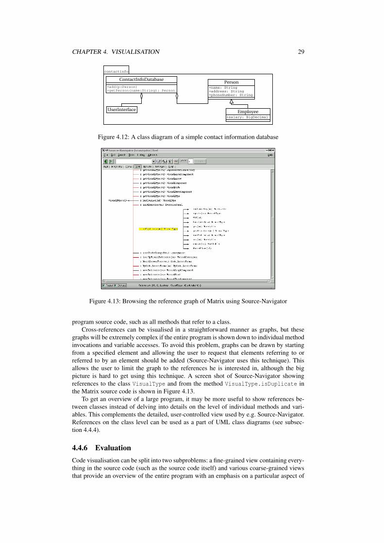
CHAPTER 4. VISUALISATION 29
contactinfo
ContactInfoDatabase
+add(p:Person)+getPerson(name:String): Person
Person+name: String+address: String+phoneNumber: String
Employee+salary: BigDecimal
UserInterface
Figure 4.12: A class diagram of a simple contact information database
Figure 4.13: Browsing the reference graph of Matrix using Source-Navigator
program source code, such as all methods that refer to a class.Cross-references can be visualised in a straightforward manner as graphs, but these
graphs will be extremely complex if the entire program is shown down to individual methodinvocations and variable accesses. To avoid this problem, graphs can be drawn by startingfrom a specified element and allowing the user to request that elements referring to orreferred to by an element should be added (Source-Navigator uses this technique). Thisallows the user to limit the graph to the references he is interested in, although the bigpicture is hard to get using this technique. A screen shot of Source-Navigator showingreferences to the class VisualType and from the method VisualType.isDuplicate inthe Matrix source code is shown in Figure 4.13.
To get an overview of a large program, it may be more useful to show references be-tween classes instead of delving into details on the level of individual methods and vari-ables. This complements the detailed, user-controlled view used by e.g. Source-Navigator.References on the class level can be used as a part of UML class diagrams (see subsec-tion 4.4.4).
4.4.6 EvaluationCode visualisation can be split into two subproblems: a fine-grained view containing every-thing in the source code (such as the source code itself) and various coarse-grained viewsthat provide an overview of the entire program with an emphasis on a particular aspect of

CHAPTER 4. VISUALISATION 30
Technique RepresentationPackage hier. Inheritance hier. References Statements
Source code p p p ppp
Package tree ppp - - -Class diagram pp ppp p -Reference graphs p - ppp p
Table 4.5: Code representations
the program, such as package trees, class diagrams and references graphs. Again, complete-ness means that everything in the code has a representation. Table 4.5 shows the evaluationof these code representation technique considered here.
4.5 Execution visualisationThe state of an executing program includes more information than the current data valuesand the source code. In particular, the current execution positions of each thread and theexecution history are of interest to the programmer.
Instead of visualising the execution history of a program directly, information aboutcauses and effects in the program can be visualised. The relationships between the causesand their effects are called the causal relationships of the program. The two most commonforms of causal relationships in a program are between assignments and reads of the samevariable and between a conditional statement and the statements caused to execute (or not)by this statement.
4.5.1 Tracing through source codeThe most usual way of representing the execution of a program in visual debuggers is bydisplaying the source code with the current line highlighted or marked in some way. Forexample, in Figure 4.10 the current line is indicated using an arrow. This approach is veryeasy to implement and is familiar to most programmers, but requires a lot of screen spaceand does not integrate very well with a graphical data view.
The parameters with which the currently executing method was called can be added tothe view (e.g. as an annotation to the formal parameters in the method header, although thismay not be visible while tracing execution).
4.5.2 Highlighting objectsWhen a method is executed, this can be displayed by highlighting the object or class towhich the method belongs in the data view and the running method. Similarly, when a fieldof a class or object is written or read, the field and the class or object to which it belongscan be highlighted.
4.5.3 Annotating objectsIf the object view does not contain the methods, they must be added to the on-screen rep-resentation of the object in order to show that they are being executed. Multiple runninginstances of the same method can be shown by mentioning the method once for every in-vocation. Information on the location on the stack and parameters of each invocation canbe shown as a part of this. The current execution position can also be shown for each activemethod. An example of this is shown in Figure 4.14.
This method can also be used to visualise the execution history of the program byannotating each object with the methods executed on it and the operations performed as

CHAPTER 4. VISUALISATION 31
123key
AVLTreeNode 54
children
height 2
2: rotateright(): 103
3: insert(int key=99): 25
Figure 4.14: Example of an object annotated with executing methods (stack position,method name, parameters and current line number)
part of these methods. However, this will quickly become hopelessly cluttered. For clarity,the operations should be grouped by executing method and only the method invocationsshould be visible by default (see discussion of elision control in Subsection 5.4.1).
4.5.4 Drawing operations as connectionsWhen an object calls another, they can be interconnected graphically (e.g. by an arrow)to show a method call. Prosasim uses this approach, which can be expressed convenientlyusing UML collaboration diagrams (see Subsection 4.5.8). This can be extended to ma-nipulation of variables. Different representations could be used for read, write and calloperations; various forms of arrows seem natural. Static method calls can be shown onthe graphical representation of the class. Some of these ideas have been implemented inVisiVue.
4.5.5 Viewing the execution stackPractically all modern programming languages have an execution stack or execution stacksof some form. The contents of an execution stack can be displayed in a number of ways.The most straightforward approach is to display the stack frames on top of each other as avertical table. This suits the stack metaphor well. Each stack frame can then be considereda special form of object (the local variables in the frame can be considered fields) anddisplayed accordingly.
This allows the user to check which methods are active and the values of all their localvariables and arguments. The current position in each method can also be added to the stackframe.
Most debuggers only show a list of calls and arguments in the execution stack view,and require the user to select a stack frame in order to view its local variables. This makesit hard to get an overview of the calls made by the program. Therefore, the local variablesor at least the parameters of the method call should be shown in the stack frame.
4.5.6 Viewing the call treeVCC [5] displays all function calls that have been made as a tree, with the currently activebranch highlighted. By pointing to a node in this tree, the arguments and local variables inthis function call can be seen.
Displaying the call tree for a thread is a generalisation of displaying the execution stack.It allows the user to examine the arguments of all calls that have been made instead of justthe currently active calls. It is also a convenient way of structuring the list of operationsperformed by the thread.

CHAPTER 4. VISUALISATION 32
Figure 4.15: An example of RetroVue’s history view based on an extended call tree
To implement the call tree display, all method calls must be stored. Also, the values oflocal variables and arguments must be stored when a method exits. This can be done bycopying stack frames whenever a method exits. Alternatively, if all local assignments arelogged, the relevant information can be reconstructed from this.
RetroVue displays the entire execution of a thread, including all operations that changedata values (e.g. assignments) as a tree structured by method calls [81]. This representationincreases the information content of the call tree significantly. An example of a tree fromRetroVue is shown in Figure 4.15.
The biggest problem with the call tree view is that it integrates badly with the data view,which makes it hard to see the connection between the objects shown in the data view andthe operations in the call tree.
4.5.7 Sequence diagramsUML sequence diagrams (described in e.g. [20]) show the flow of control and interactionbetween objects in an object-oriented program. In these diagrams, time is represented bythe Y axis. They show objects as vertical lines with a box identifying the object at thetop and boxes along the lines indicating execution and arrows between objects indicatingmessages between objects.
Only calls are usually considered messages. However, all operations can be shown asmessages, at the expense of adding large numbers of messages from objects to themselves.
Sequence diagrams can be used to visualise the execution flow of a running program. Asa sequence diagram of the entire execution of a program is going to be unmanageably largein most realistic cases, the user must specify the part of the execution of the program toview. One way to do this is by selecting a branch from the call tree. The sequence diagramcan then easily be generated from the information in the call tree. Sequence diagrams canbe used to display multiple threads that communicate using asynchronous calls [34]. Anexample of a sequence diagram is in Figure 4.16.

CHAPTER 4. VISUALISATION 33
UserInterface ContactInfoDatabase newPerson : Person
<<create>>
addPerson(newPerson)
Figure 4.16: A sequence diagram of an insertion in the database shown in Figure 4.12
4.5.8 Collaboration diagramsUML collaboration diagrams (in e.g. [20]) are another way to show interaction betweenobjects. These diagrams show objects as boxes and messages (e.g. method calls) betweenthem as arrows. The order and type of the messages is specified by labelling the arrows.The message type and parameters are shown as labels on the arrows.
The arrow labels include a sequence number for the message, the message (includingits parameters) and (where applicable) a list of preceding messages in other threads [41].Thus, collaboration diagrams can be used to show the operation of multithreaded programs,including the interaction between threads.
A collaboration diagram is more suitable for describing interactions between severalobjects than a sequence diagram. On the other hand, the order in which things happen ismuch clearer in a sequence diagram. Moreover, collaboration diagrams occupy less screenspace than sequence diagrams.
Like sequence diagrams, collaboration diagrams are easily constructed from branchesof a call tree. If the currently executing branch of the program is shown as a collabora-tion diagram, the resulting dynamic collaboration diagram is similar to drawing arrows formethod calls (as described in subsection 4.5.4), but with numbering and without removingthe arrows after the call is completed.
By displaying all operations as messages, collaboration diagrams can be extended toshow all operations that occur, although this makes the diagram extremely cluttered.
4.5.9 Hybrid diagramsThe message passing arrows of a collaboration diagram can also be used to display callsand interactions between objects in a data view that shows the relevant objects, whicheliminates the need for a separate collaboration diagram. Annotations can be used to displayoperations, statements or source code lines executed by an object and the current executionposition in running methods. The resulting hybrid diagram describes both the state of theprogram and its execution history, but it may easily become cluttered and it is not in theUML.
As with annotation of objects, the operations performed by each invoked method mustbe elided by default to keep the amount of information shown manageable (see Subsec-tion 5.4.1 for details).
An example of a hybrid diagram (depicting an AVL tree insertion interrupted just beforerotating, with all executed instructions elided except for one of the currently executinginsert method invocation) is shown in Figure 4.17.

CHAPTER 4. VISUALISATION 34
insert(99)
1: insert(99)
123key
1.2: 24: if (children[0]!=null)
1.7: 30: rotateright();1.6: 29: if (rh−lh<−2)1.5: 28: lh=children[0].height;1.4: 27: rh=children[1].height;
1.1: 23: if (key<this.key)
insert(int key=99): 25
1.3: 25: children[0].insert(key);
key 100
1.3: insert(99)
1.3.1: insert(99)
1.3: insert(99)
1.7: rotateright()
AVLTreeNode 12
AVLTreeNode 23 key 150
AVLTreeNode 63
AVLTreeNode 98
AVLTreeNode 87
children
height 2
height
children
0
insert(int key=99): 30
key 110
1
1: insert(99):
1.7: rotateright(): 103
children
height
children
height 1
1.3.1: insert(99)
key 99
children
height 0
Figure 4.17: An example of a hybrid diagram

CHAPTER 4. VISUALISATION 35
4.5.10 Assignment searchA simple way to allow the user to find the reason for the value of a variable is to searchbackwards through the execution history of the program for the last assignment to a vari-able. The result of this search is the statement that gave the variable the value it has at thecurrent point of execution.
By searching through the execution history instead of attempting static analysis, sideeffects of e.g. method calls are automatically taken into account.
If the program is multithreaded in such a way that multiple operations can occur simul-taneously on the same variable, it may be impossible to define a total ordering of read andwrites on a variable. If variable reads and writes are atomic, this problem does not arise.In Java, read and write operations on double and long variables may be non-atomic [36].This means that assignment search in Java programs may fail on double and long variablesunless additional locking is introduced.
4.5.11 Slicing and dependence graphsWhen looking for reasons for a program’s misbehaviour, many programmers look at the(incorrect) value of a variable and try to find a reason for this value by tracing the executionof the program backwards. In essence, they try to concentrate on the part of the programthat could have affected the variable value. Parts of programs that could have affected thevalue of a specified variable at a specified statement or point in the execution of a programare called slices and the process of calculating slices is called slicing. [60]
Definitions
Slicing uses techniques from data and control flow analysis to determine the statements thatcould have affected the value of a variable at a specified statement or point in the executionof the program. This is either done by static analysis, in which case the slice (a static slice)contains all the statements that can affect the value of the variable at the specified statement,or by dynamic analysis based on a specified execution history, in which case the slice (adynamic slice) contains all the statements in the execution history that could have affectedthe value of the variable at the end of the execution history. In other words, the static sliceis based on any possible execution history, while the dynamic slice is based on a specificexecution history.
Slices are defined using dependence graphs. A static slice is based on a program de-pendence graph (PDG), while a dynamic slice is based on a dynamic dependence graph(DDG).
Definition 1 Program dependence graph (PDG):A PDG is a directed graph. The vertices of a PDG are the statements in a program. An edgeexists in a PDG from x to y iff x 6= y and one of the following is true:
• x has a (static) data dependency on y, i.e. y writes to a variable, memory location orsuch that may be read by x.
• x has a (static) control dependency on y, i.e. x executes or does not execute dependingon the path taken at a conditional branch at y.
Definition 2 Dynamic dependence graph (DDG):A DDG is a directed graph. The vertices of a DDG are executed statements (one vertex forevery time a statement is executed), and an edge exists from x to y iff x 6= y and one of thefollowing is true:
• x has a (dynamic) data dependency on y, i.e. x read a value written by y.

CHAPTER 4. VISUALISATION 36
• x has a (dynamic) control dependency on y, i.e. y is the conditional branch thatbranched in such a way that x was executed and another choice at y would haveallowed x to possibly not execute.
Definition 3 Static slice:A static slice at statement e with respect to variable v is the set of statements reachablealong the PDG from any statement s that can assign a value to v such that s is reachablefrom e without passing through any statement that assigns a different value to v [1, 2].
Definition 4 Dynamic slice:A dynamic slice at the end of an execution history E with respect to variable v is the setof statements reachable along the DDG from the last statement in E to assign a value tov [1, 2].
In order for these definitions to work in multithreaded programs, the order of readand write operations must be defined for each variable; no operations of this type mayoccur simultaneously. As noted in Subsection 4.5.10, this is not necessarily true in Javawithout additional locking. In most programming languages, including Java, control flowin a thread can only be affected by conditional statements in that specific thread, whichmeans that multithreading causes no additional problems for control dependencies.
Applications
Slices can be used to help a programmer locate parts of a program that may contain a fault,by allowing the programmer to select a variable in a statement and see the slice of theprogram with respect to the variable at this statement (e.g. by highlighting the slice in thesource code display). This is used in Spyder [1] and Bandera [18].
Dynamic slices are (usually) smaller than static slices, and are therefore easier to workwith when debugging [59].
By adding a few assignment statements to model method calls, object creation and otheroperations, DDGs can be defined for execution histories of object-oriented programs [64].
Slices often consist of a few statements scattered here and there in a program [60].Displaying these statements by highlighting them in the source code is not very convenient,as the user must still look for the relevant statements in the source code. Furthermore, theslice contains only a small part of the information in the PDG or DDG. The highlightedstatements correspond to the vertices of the graph, but the edges are not shown in any way.In other words, most of the information on dependencies between statements is lost whenthe dependency graph is converted into a slice.
The PDG may contain a vertex for every statement in a program, and is therefore prob-ably too large to show completely. The DDG is in most cases even larger, as it can containany number of vertices for each statement in the program; its size is only limited by thelength of the execution history. However, the DDG provides information that is specific toa particular execution history, so it reflects the real behaviour of the program more closelythan a PDG and thus suits visual testing better.
In most cases, the visualisation of a DDG must be limited to only a small part of thegraph. The definition of a dynamic slice suggests that a good starting point is the laststatement in an execution history to assign a value to a specified variable. Initially, thevisualisation of the DDG only displays the vertex corresponding to this statement. The usercan then select vertices and request that all edges from this vertex and the vertices at theends of these edges be shown. This essentially means that the user can choose an incorrectvariable value and then backtrack through the statements that could have affected the valueto find the cause of the error.

CHAPTER 4. VISUALISATION 37
Graphical layout
Definition 2 implies that if an edge exists from x to y, y was executed before x. Obviously,this precludes the existence of cycles in the DDG (an event cannot precede itself). There-fore, by placing statements in chronological order from top to bottom1, a DDG can be laidout in such a way that if x depends on y, x is always below y. This makes the order ofexecution much clearer and makes arrowheads on the edges redundant (although includingthem may improve clarity).
In multithreaded programs, chronological order may only be a partial order (i.e. somestatements have executed simultaneously so that none precedes any of the others). As-suming the assumptions made when defining a DDG hold, this poses no problem; anytotal ordering consistent with the chronological partial ordering can be used. Alternatively,statements that executed simultaneously can be shown at the same vertical position.
Application to Java programs
Constructing a DDG for a Java program appears to require modifying the JVM to keep trackof dynamic dependencies. Also, displaying the execution of a Java program as a sequenceof bytecode operations is not very useful, so the compiler should be extended to producea mapping from bytecode to source code statements [59]. As a substitute for statements,source code lines can be used, although this will decrease the detail level of the view ifseveral statements are written on a single line. Also, the bytecode instructions are at a verylow level, so combining several bytecode operations into a single vertex in the DDG shouldimprove the readability of the resulting graph. This can be done e.g. by treating a statementor a line as a single operation. In some cases, however, the option to break a complexexpression evaluation into simple parts may be useful. Therefore, it is probably a good ideato allow the user to choose between using bytecode operations, statements and lines as thevertices of the DDG.
Most Java bytecode operations manipulate an operand stack that is specific to eachexecution stack frame. If bytecode operations can be observed individually, the locationson the operand stack can be treated as variables in the DDG.
Control dependencies can be calculated either by analysing the source code or the byte-code. When analysing the source code, the dependencies are more or less determined bythe block structure of the source code. When analysing the bytecode, an algorithm thatcomputes control dependency graphs for any control flow, such as the algorithm describedin [19] and [4], must be used. However, analysing the bytecode has the distinct advantagethat the bytecode has only a few simple operations that affect control flow, while the sourcecode is more complex and may be optimised by the compiler.
The control flow in Java programs is complicated by two additional issues: exceptionsand concurrency.
Exceptions make the control flow more complex, as exceptions can be caught in anyof the calling methods and they can cause methods to terminate prematurely. Control flowgraphs can be extended to include exception handling [51]. However, this extension makesthe control flow graphs larger and harder to generate. For the purposes of visualisation itmay be a better idea to ignore exceptions until one is actually thrown rather than clutter thedependency graph by adding the possibility of an exception being thrown to every time afield or method in an object is used; after all, a NullPointerException could be generatedby any one of these operations. Similarly, every single read or write of an array element cancause an ArrayIndexOutOfBoundsException and every integer division or remainder cancause an ArithmeticException unless the indices or divisors can be shown to be alwaysvalid (which is hard to do in most cases). To ignore exceptions until they are actuallythrown, one need merely ignore them when calculating control dependencies except formaking the execution of the catch clause that catches the exception control dependent on
1Obviously, this layout can be mirrored, rotated and otherwise transformed in a number of ways.
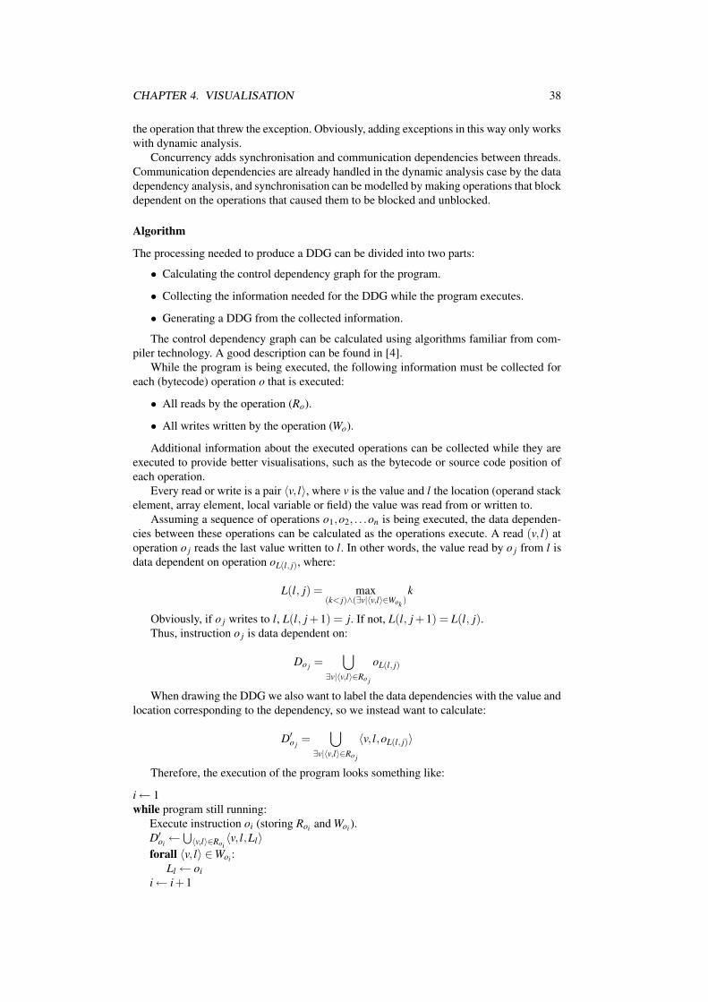
CHAPTER 4. VISUALISATION 38
the operation that threw the exception. Obviously, adding exceptions in this way only workswith dynamic analysis.
Concurrency adds synchronisation and communication dependencies between threads.Communication dependencies are already handled in the dynamic analysis case by the datadependency analysis, and synchronisation can be modelled by making operations that blockdependent on the operations that caused them to be blocked and unblocked.
Algorithm
The processing needed to produce a DDG can be divided into two parts:
• Calculating the control dependency graph for the program.
• Collecting the information needed for the DDG while the program executes.
• Generating a DDG from the collected information.
The control dependency graph can be calculated using algorithms familiar from com-piler technology. A good description can be found in [4].
While the program is being executed, the following information must be collected foreach (bytecode) operation o that is executed:
• All reads by the operation (Ro).
• All writes written by the operation (Wo).
Additional information about the executed operations can be collected while they areexecuted to provide better visualisations, such as the bytecode or source code position ofeach operation.
Every read or write is a pair 〈v, l〉, where v is the value and l the location (operand stackelement, array element, local variable or field) the value was read from or written to.
Assuming a sequence of operations o1,o2, . . .on is being executed, the data dependen-cies between these operations can be calculated as the operations execute. A read (v, l) atoperation o j reads the last value written to l. In other words, the value read by o j from l isdata dependent on operation oL(l, j), where:
L(l, j) = max(k< j)∧(∃v|〈v,l〉∈Wok )
k
Obviously, if o j writes to l, L(l, j +1) = j. If not, L(l, j +1) = L(l, j).Thus, instruction o j is data dependent on:
Do j =⋃
∃v|〈v,l〉∈Ro j
oL(l, j)
When drawing the DDG we also want to label the data dependencies with the value andlocation corresponding to the dependency, so we instead want to calculate:
D′o j=
⋃
∃v|〈v,l〉∈Ro j
〈v, l,oL(l, j)〉
Therefore, the execution of the program looks something like:
i← 1while program still running:
Execute instruction oi (storing Roi and Woi).D′oi←
⋃〈v,l〉∈Roi
〈v, l,Ll〉
forall 〈v, l〉 ∈Woi :Ll ← oi
i← i+1

CHAPTER 4. VISUALISATION 39
a=
a=4
+
a
b
if <
b+=1
a=
+
a
b
a=
1
b=
1
if <
b
3
b
3
4
22
b=22
3
a=2
b=2
1
1a=1
b=1
b=1
1
3
b=1
1 1
2
Figure 4.18: A bytecode operation-level DDG
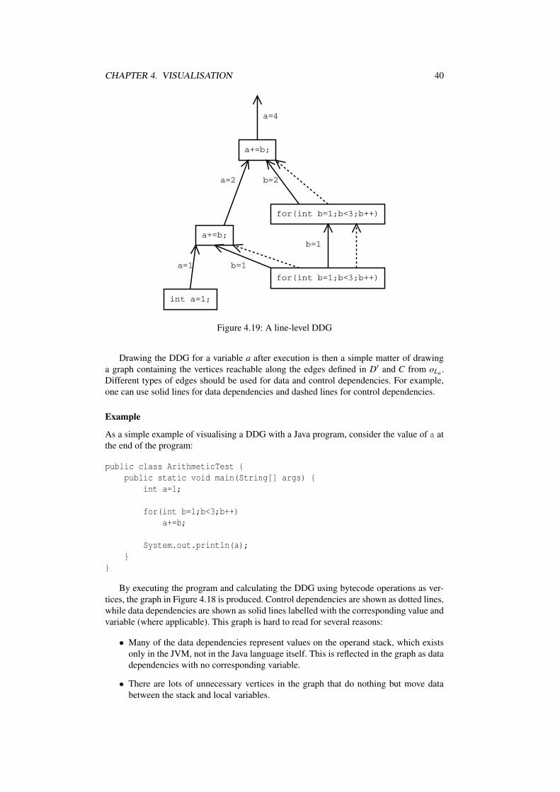
CHAPTER 4. VISUALISATION 40
a+=b;
a+=b;
int a=1;
for(int b=1;b<3;b++)
for(int b=1;b<3;b++)
a=1
a=2
a=4
b=1
b=1
b=2
Figure 4.19: A line-level DDG
Drawing the DDG for a variable a after execution is then a simple matter of drawinga graph containing the vertices reachable along the edges defined in D′ and C from oLa .Different types of edges should be used for data and control dependencies. For example,one can use solid lines for data dependencies and dashed lines for control dependencies.
Example
As a simple example of visualising a DDG with a Java program, consider the value of a atthe end of the program:
public class ArithmeticTest {public static void main(String[] args) {
int a=1;
for(int b=1;b<3;b++)a+=b;
System.out.println(a);}
}
By executing the program and calculating the DDG using bytecode operations as ver-tices, the graph in Figure 4.18 is produced. Control dependencies are shown as dotted lines,while data dependencies are shown as solid lines labelled with the corresponding value andvariable (where applicable). This graph is hard to read for several reasons:
• Many of the data dependencies represent values on the operand stack, which existsonly in the JVM, not in the Java language itself. This is reflected in the graph as datadependencies with no corresponding variable.
• There are lots of unnecessary vertices in the graph that do nothing but move databetween the stack and local variables.
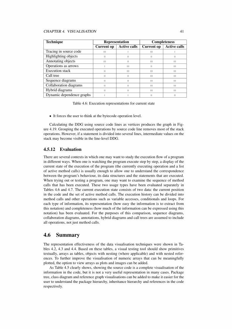
CHAPTER 4. VISUALISATION 41
Technique Representation CompletenessCurrent op Active calls Current op Active calls
Tracing in source code ppp p ppp p
Highlighting objects pp pp pp pp
Annotating objects ppp pp ppp ppp
Operations as arrows p ppp pp ppp
Execution stack pp ppp ppp ppp
Call tree pp pp ppp ppp
Sequence diagrams pp pp ppp ppp
Collaboration diagrams pp pp ppp ppp
Hybrid diagrams pp pp ppp ppp
Dynamic dependence graphs p p pp pp
Table 4.6: Execution representations for current state
• It forces the user to think at the bytecode operation level.
Calculating the DDG using source code lines as vertices produces the graph in Fig-ure 4.19. Grouping the executed operations by source code line removes most of the stackoperations. However, if a statement is divided into several lines, intermediate values on thestack may become visible in the line-level DDG.
4.5.12 EvaluationThere are several contexts in which one may want to study the execution flow of a programin different ways. When one is watching the program execute step by step, a display of thecurrent state of the execution of the program (the currently executing operation and a listof active method calls) is usually enough to allow one to understand the correspondencebetween the program’s behaviour, its data structures and the statements that are executed.When trying out or testing a program, one may want to examine the sequence of methodcalls that has been executed. These two usage types have been evaluated separately inTables 4.6 and 4.7. The current execution state consists of two data: the current positionin the code and the set of active method calls. The execution history can be divided intomethod calls and other operations such as variable accesses, conditionals and loops. Foreach type of information, its representation (how easy the information is to extract fromthis notation) and completeness (how much of the information can be expressed using thisnotation) has been evaluated. For the purposes of this comparison, sequence diagrams,collaboration diagrams, annotations, hybrid diagrams and call trees are assumed to includeall operations, not just method calls.
4.6 SummaryThe representation effectiveness of the data visualisation techniques were shown in Ta-bles 4.2, 4.3 and 4.4. Based on these tables, a visual testing tool should show primitivestextually, arrays as tables, objects with nesting (where applicable) and with nested refer-ences. To further improve the visualisation of numeric arrays that can be meaningfullyplotted, the option to view arrays as plots and images can be added.
As Table 4.5 clearly shows, showing the source code is a complete visualisation of theinformation in the code, but it is not a very useful representation in many cases. Packagetree, class diagram and reference graph visualisations can be added to make it easier for theuser to understand the package hierarchy, inheritance hierarchy and references in the coderespectively.

CHAPTER 4. VISUALISATION 42
Technique Representation Completeness CausalCalls Other ops Calls Other ops
Tracing in source code p p p p p
Highlighting objects pp pp p p p
Annotating objects p pp ppp ppp pp
Operations as arrows pp pp p p p
Execution stack pp pp p p p
Call tree ppp pp ppp ppp pp
Sequence diagrams pp pp ppp ppp pp
Collaboration diagrams pp pp ppp ppp pp
Hybrid diagrams pp ppp ppp ppp pp
Dynamic dependence graphs pp pp pp pp ppp
Table 4.7: Execution history representations
Tables 4.6 and 4.7 suggest that showing the execution stack, displaying the executionhistory as a call tree and hybrid diagrams, tracing execution in the source code and brows-ing the dynamic dependence graph is sufficient for satisfactory visualisation of execution.This means that additional visualisations such as viewing operations as arrows, collabo-ration diagrams, highlighting or annotating objects and sequence diagrams are not reallynecessary, although some special cases may exist in which they are more convenient.

Chapter 5
Elision and abstraction
Elision (hiding unwanted information) and abstraction (hiding nonessential aspects of in-formation such as implementation details) are the two key techniques used to keep theamount of information in a program manageable.
In well-written object-oriented code, abstraction and encapsulation are used to ensurethat the functionality of a module of the code can be used, without being aware of theimplementation of the module, through an interface that captures the essentials of the func-tionality of the module [26]. The goal of data abstraction in visual testing is to ensure thatdata structures can be viewed in a fashion consistent with their interfaces instead of theirimplementations in cases where the implementation is irrelevant.
The data, code and execution history views should all work with large amounts ofinformation, and it therefore becomes necessary to provide convenient ways for the user tochoose which information is shown. In other words, the data, code and execution historyviews need elision control.
Abstraction and elision techniques are evaluated using the point system described inTable 5.1.
5.1 Data abstractionAbstraction of implementation details is necessary to keep a data view of a nontrivial pro-gram from becoming a bewildering mess of objects and references. Generally speaking, theuser should have control over the degree of abstraction in order to help him concentrate onthe parts of the program that he is working on instead of the internals of libraries.
The abstract data structures must be capable of referring to other data structures andother data structures must be able to refer to both the abstract data structures and other datastructures inside them. In order to allow this, the abstraction must not break apart objectsor classes into separate parts, as this makes it hard to refer to the object from elsewhere. Asmost abstract data structures will probably be implemented as objects or groups of objectsof the same or similar classes, it makes sense to have the data abstracter receive an object
Score Meaning- The technique does not do anything to satisfy this criterion.p The technique does not satisfy the criterion on its own, but does some-
thing that is useful with regard to the criterion.pp The technique satisfies the criterion reasonably well in many cases.ppp The technique satisfies the criterion very well.
Table 5.1: Scoring system for evaluation of elision and abstraction techniques
43

CHAPTER 5. ELISION AND ABSTRACTION 44
and work out a representation for it.In visual testing, producing an abstract data view consists of two tasks:
• Identifying the data structures that should be abstracted and the abstraction to use foreach data structure.
• Converting the data to the abstracted form.
5.1.1 Identification by class or interfaceIn languages with an extensive standard library, such as Java, a large amount of useful datastructures and interfaces are readily available to the programmer. Because of this, manyJava programs use the standard data structures to provide convenient implementations ofabstract data types. Recognising the classes that implement these data structures, which arepart of the Java API standard [57], allows a large amount of data structure implementationdetails to be abstracted away. In this fashion, several data structures that can reasonablybe displayed as arrays or lists, e.g. java.util.HashSets and java.util.LinkedLists,can be shown as arrays or lists instead of displaying their underlying implementation asdebuggers usually do.
Essentially, the user has, in writing the program, explicitly marked several commonADTs (abstract data types) and FDTs (fundamental data types) as such. Not making use ofthis added information would be wasteful.
Although program visualisers usually use type definitions to determine the appear-ance of objects, most of them do not make use of prior knowledge of standard libraryroutines. Instead, many of them (e.g. Eliot [58] and the Korsh-LaFollette-Sangwan sys-tem [32, 33, 50]) require the inclusion of special type definitions in the user program.However, Tarraingím uses the interfaces of objects to monitor changes to the objects andexamine the objects [40].
Naturally, this technique can be generalised to data structures created by users, althoughthis shifts the responsibility for adding support for the data structures to the visual testingtool onto the user.
Collections
Any object that implements the java.util.Collection interface can be considered agroup of objects [57]. This group of objects can be shown as a list or a table. The imple-mentation details of library classes that implement java.util.Collection are usually ir-relevant from the programmer’s point of view, and should be hidden by default. To provideadditional functionality, some of the implementations and subinterfaces of Collection,such as Set and List, can have separate abstractions adapted to their specific properties.
Maps
The java.util.Map interface lends itself to abstraction in a similar way to Collection.The simplest visualisation is as a list of pairs, in which each pair consists of a key anda value (an object reference which can be displayed as a reference or a nested object, asusual).
Wrapper classes for primitives
The wrapper classes for primitives in java.lang can be shown as the primitives they con-tain.
Plots
The plots discussed in section 4.2.3 can also be considered abstractions of arrays.

CHAPTER 5. ELISION AND ABSTRACTION 45
Graphics
Graphical objects (such as java.awt.Images or objects that have a paint method thatdraws the object onto a specified java.awt.Graphics object) can be displayed graphi-cally, instead of as objects. The paintmethod is used in subclasses of java.awt.Componentto define the appearance of components, so the easiest way to detect this is to look for sub-classes of java.awt.Component.
Many of these objects will probably be quite large, and in many programs most of themwill probably be user interface objects with unchanging appearance. Cluttering the viewwith these by default is probably not a good idea.
Sound
Sound files, such as javax.sound.sampled.DataLines and javax.sound.midi.Sequences,can be shown as objects with “play” and “stop” buttons, which start and stop playback ofthe sound. This can even be generalised to video clips, although this is probably not veryuseful.
This addition is useless when debugging programs that do not process sound, so it isnot very important.
5.1.2 Identification by patternsUWPI [23] attempts to recognise ADTs by looking for recognised patterns of use; by exam-ining how the CDT is used, it can determine what ADT it implements. While Java simplifiesthis process by encouraging the limitation of access to variables, it also provides predefineddata types, either in the language or in the standard library, for many of the ADTs recog-nised by UWPI. Also, the type inference used by UWPI is inherently ambiguous in manycases. Furthermore, UWPI’s data type inferencer concentrates on recognising different usesof integers as e.g. Boolean variables or pointers, where a Java programmer would probablyuse boolean variables and references. UWPI is therefore better suited for languages witha limited set of primitives such as Pascal, C or C++.
This approach is not very useful on its own in Java, although it could be used as anadjunct to recognising known structures. For example, a tree can be constructed in Javaby having a class of node objects, each of which contains a set of child elements. Here,determining that the nodes form a tree requires determining that each node contains a setof references to other nodes. To do this, we must first identify the set as such, and thencheck that it only contains references to other nodes. Finally, the graph expressed by thereferences must be shown to be connected and acyclic (if not, the resulting graph is not atree). This poses a problem as the contents of the tree must be known in order to verifythese properties of the references. Also, a structure that at one point appeared to be a treemay later be found to contain a cycle.
Because of the risk of incorrectly identifying structures by allowing differentiationbased on properties that may change over time (for example, adding an edge may con-vert a tree into a graph with a cycle), it seems best to limit this abstraction mechanism tostatic analysis of the classes.
Linked lists
Linked lists have a simple structure: they consists of nodes that contain a link to anothernode (the next node) and some other data (usually a reference to a content object). Themajor problem with identifying linked lists based on their structure is that the references tothe following objects may induce a cycle. Furthermore, several different objects may havethe same next object, in which case the structure can be any graph where the out degreeof every vertex is 1. Although identifying linked lists and displaying them as tables wouldprovide a more compact representation for an easily implemented data structure, it is hard

CHAPTER 5. ELISION AND ABSTRACTION 46
to prove that the lists stay separated from each other. Alternatively, if a node is referred tofrom several different places, copies of the list can be shown in all of these places.
If a graph-like representation for references is used, linked lists will automatically beshown as chains of elements without any of the problems mentioned above. The visuallayout may, however, not take into account that the linked nodes form a list.
In Java, it is arguably bad programming practice to implement linked lists that do notconform to the java.util.List interface, so there is little reason to attempt to detectlinked lists based on their structure.
Trees and graphs
Trees and graphs are usually represented using nodes containing lists of children or neigh-bours (adjacency lists). If references between objects are drawn using arrows betweenboxes, graphs and trees of this type are automatically shown as graphs.
An adjacency matrix can easily be drawn as a graph; however, if one wishes to showthe nodes as anything other than integer indices, a vertex data array must also be specified.Similarly, if adjacency lists are constructed using integer node indices, a mapping fromindices to nodes must be specified. Specifying these mappings must in practice be donemanually. For trees or graphs limited to a specific structure (e.g. binary trees), there may beseveral separate variables that form the adjacency lists. Otherwise, the situation is the sameas for the general form. In conclusion, there seems to be little need to detect trees or graphsautomatically.
5.1.3 Accessors and modifiersIn Java programming (and to some extent in other object-oriented languages), it is consid-ered good programming style to provide access to data stored in objects through methodsinstead of allowing public access to fields. In fact, many books on object-oriented program-ming (such as [26]) and even the Java language specification [21] insist on this, as it allowsmuch better abstraction and encapsulation than direct field access. One method (called anaccessor) reads the value, and another (optional) method (a modifier) writes it. These areusually of the form1 (for a value called myValue of type Value):
Value getMyValue(); /* An accessor. */void setMyValue(Value v); /* A modifier. */
Part of the time, accessors and modifiers are used to enforce access limitations on afield. For example, to allow any class to read the value, but only subclasses and classesin the same package to write to the value, one need merely make the variable storing thevalue private, the accessor public and the modifier protected. Modifiers are also usedto check the validity of new data values before modifying object fields.
However, in some cases, accessors and modifiers may allow manipulation of a datavalue in a different form than the form in which it is stored. For example, the toStringmethod in any Java object reads the data in the object and outputs it as a string. In thesecases, it may be more convenient to access the data using these methods rather than directlyaccess fields of the object. Essentially, these methods provide a way for the programmerto easily access a value that cannot be accessed directly by reading and writing a variable.Also, accessors and modifiers can be used to provide a common interface to data that canbe stored in many different ways using different types of objects. By supporting this typeof data access in a visual testing tool, we allow the user to examine his data in the same
1Actually, the naming conventions for accessors in [21] differ depending on the intended meaning of theaccessor. For example, an accessor that is supposed to convert the entire contents of an object into a value of typeType is called toType. These other forms of accessors can be identified using the same techniques as the simplecase described here.

CHAPTER 5. ELISION AND ABSTRACTION 47
way that he manipulates it in the code he is working with by exploiting an abstraction thatis already defined in the program code.
Accessors and modifiers can easily be identified if they are of the simplest possibleform (where field is a field of this):
private Value field;
Value getValue() {return field;
}
void setValue(Value v) {field=v;
}
Recognising methods of this type provides no information except that it shows thata private field actually may be accessible outside the class in which it is defined. Thisinformation may be useful for elision purposes, as it provides an easy way to distinguishbetween private fields intended for internal state and private fields intended to be visibleoutside the package through an accessor. However, this information provides no additionalabstraction.
If field can be a chain of fields (e.g. obj1.obj2.fld), a larger group of methods canbe recognised, although changing one of the object references in this chain changes thefield manipulated by the methods.
In the general case, the value manipulated by the accessor/modifier pair can be storedin a huge number of ways; it can be split, combined with other variables, compressed, en-crypted, serialised, converted, and so on. However, the method pair still has the propertythat calling the accessor after calling the modifier returns the value passed as the parame-ter to the modifier. Identifying accessors and modifiers that do complicated processing onvalues and still have this property is a lot harder; for example, proving mathematical equa-tions is actually a subproblem if arithmetic operations are allowed. Some simpler cases areanalysable, such as those where data flow analysis allows one to prove that if getValue()is immediately preceded by setValue(v), the value returned is always v. However, thesecases only constitute a subset of the set of accessor and modifier pairs, and performing thedata flow analysis is complex, although it is a well known problem in compiler design.Also, this technique cannot be used to identify accessors that do not have correspondingmodifiers.
On the other hand, simply accepting every pair of methods with the right return andparameter types will probably yield a lot of false positives. The simplest method of filteringout false positives is to assume that the user’s code follows the common naming conventionof calling the modifier set〈value〉 and the accessor get〈value〉 for any name 〈value〉.
Another criterion for an accessor is that it has no side effects; in other words, it doesnot change the state of any object. Specifically, the method and all the methods it callscontain no assignments to non-local variables. Checking this property requires parsing thepotential accessor (either as source code or bytecode) and the code of all the methodsit calls and ensuring that all variables that are set are local. This is quite a complicatedsolution, and it does not take into account the possibility of multiple counteracting sideeffects. However, when extracting data values to show in a debugger, a lack of side effectsis a very useful property, as the debugger may execute the accessor at any time. Obviously,executing methods with side effects in a nondeterministic fashion (from the debuggee’spoint of view) is a good way to introduce new problems.
The ideas presented here for accessor/modifier pairs can also be applied to another com-mon idiom: methods that add and remove items from collections and return the collectionor an iterator for it. The problems with identifying these methods are more or less the sameas for accessors and modifiers.

CHAPTER 5. ELISION AND ABSTRACTION 48
If read-only access is sufficient, the identification process can be limited to identifyingaccessors by looking for methods that return a value and have no arguments or side effects.This can be done automatically.
The values manipulated by accessors and modifiers can be considered equivalent tofields for the purposes of visualisation. As these values do not always represent the contentsof real data fields, I will refer to them as virtual fields.
Executing accessors or modifiers on an object while it is being modified may causeinvalid results, infinite loops, deadlocks or exceptions to occur in the accessor or modifierif the accessors and modifiers are not thread-safe. If they are thread-safe (and no thread-unsafe operations are being performed on the object), the accessor or modifier may onlydeadlock. Deadlocks and other aberrant behaviour can be avoided by running the accessoronly when it is known to be safe to do so. For a properly designed object with accessors andmodifiers, it is always safe to run an accessor or modifier when no other method is runningon the object.
When using logging, virtual fields generated by accessors can only be shown reliablyfor historical data if the accessor was executed and its return value was stored at the timethe data was current.
5.1.4 User-defined abstractionIn ambiguous cases (e.g. a tree implemented using a map from each node to its parent, anarray that can either be viewed as a table or a graph or an accessor/modifier pair), caseswhere the actual implementation of a data structure is interesting, or cases where a newknown structure is introduced, the user may want to specify a different representation thanthe default. A list of possible interpretations of a data structure (including the default gen-eral representation for unidentified objects) can be used for this.
The user may also wish to specify which fields of an object form the parts of the datastructure (for example, in a map, the user may need to specify which field contains the keysand which contains the values). In order to do this, the user must also point out the variablesthat form the parts of the abstract data structure.
Many program visualisation systems rely heavily on manual identification and map-ping of data structures to visualisation operations (e.g. Lens and Leonardo [16, 37, 38]).The mapping can be specified using a graphical user interface (as in Lens) or using a pro-gramming language (as in Leonardo).
Manual identification is very flexible, but it easily becomes time-consuming and error-prone if visualisations and abstractions cannot be reused easily. These problems are exac-erbated if the visualisation is programmed as a part of this process. For example, Lens isnot well suited for debugging for this reason [24].
Lifted fields
Instead of displaying the value of a field of an object, the user may wish to display thevalue of a field of an object that can be reached by following references in the object to bedisplayed. The user should be able to produce a chain of fields to traverse until the desiredfield is found; this field can then be shown in the object to be displayed as a virtual field. Inother words, a field is lifted out from a referenced object, producing a lifted field.
5.1.5 Combining abstractionsWhen visualising complex data structures, it is important to be able to combine abstrac-tions. This allows the user to easily create complex abstractions that would otherwise re-quire additional code.

CHAPTER 5. ELISION AND ABSTRACTION 49
In order to do this, abstractions should be designed to read and write data in the sameform as the visualiser. This means that any abstraction that can be visualised can also beused as part of a combined abstraction.
As an example consider showing the attributes of an XML element using the DOM(Document Object Model) API (a part of the standard Java API [57]). The attributes arereturned as a map containing attribute objects with names and values. Using two accessorvirtual fields, the names and values of the attributes can be extracted as fields. The map canbe converted to a table of attributes by specifying the methods to get the table length andan item in the table. This table of pairs can then be interpreted as a map by specifying thefields of the pairs to use.
5.1.6 Data abstraction modelThe abstraction techniques described in this section can be expressed using virtual fieldsand convertors. Convertors output objects that implement the interface of one data typebased on the data in an object of another type. For example, the abstraction for Collectionsdescribed earlier can be implemented as a convertor that outputs a table and uses theCollection interface to read and write elements.
Convertors can have settings that determine how they interpret the structure they convertfrom and properties of the structure they convert to. For example, a convertor that producesan array from a structure with methods to get and set an element has at least three settings:the two methods to use and the field to read the length from. A convertor applied to aspecific type of data structure with specified settings can be considered an interpretation ofthe real data structures. By applying convertors only when necessary, a lot of storage andprocessing can be avoided.
All virtual fields can be rewritten as a field containing a suitable convertor. Therefore,only one single virtual field type is necessary: a converted field.
An interpretation defined for objects of a class is also valid (syntactically, at least) forobjects of its subclasses. Similarly, an interpretation defined for an interface is valid forclasses that implement it. This means that the interpretations defined for the ancestors ofa class (the ancestors of a class or interface are its superclass, the interfaces it implementsand their ancestors) can be used for the class. Similarly, if no default interpretation has beenspecified for a class, the default interpretation of any of its superclasses or interfaces canbe used.
Deciding which ancestor’s default interpretation should be used is not trivial. However,a few useful rules of thumb can be devised:
• If a class has its own specific interpretation, it is usually better suited for that class andits subclasses than any ancestor’s view. Similarly, the interpretation of an interface isbetter for classes that implement the interface or a subinterface of the interface thanthe interpretation of a superinterface of the implemented interface.
• If a class is similar to the class for a which a visualisation is defined, the visualisationwill probably work reasonably well.
Thus, assuming we can quantify “similarity” (or conversely, “dissimilarity”) betweentwo classes or a class and an interface, we have an ordering on the suitability of interpreta-tions of ancestors, and can choose the most suitable interpretation. One possible definitionof dissimilarity between a class and a superclass of it is the amount of overridden or addedmethods. The dissimilarity to an interface can be defined as the amount of added methods.
To allow the user to switch between different valid interpretations of an object easily,each class should have a set of defined interpretations. The user can then easily choosewhich one is used for visualisation. If these interpretations are identified by name, they canbe used as input for convertors to combine abstractions wihout affecting the visualisation.

CHAPTER 5. ELISION AND ABSTRACTION 50
Technique Abstraction Auto view control Manual view controlIdentification by class/interface pp pp p
Identification by patterns p pp -User-defined abstractions ppp - pp
Table 5.2: Data type identification techniques
5.1.7 EvaluationProducing a data representation with abstraction involves two tasks: identifying the datastructures and converting them into a suitable form.
All the identification techniques examined here require manual definition of some formof rules for the recognition of implementations of a data structure as well as a suitable vi-sualisation for the data structure. The different approaches only differ in how much of thework is done by the user (reflected in the automatic view control rating), how well the usercan adapt the visualisation to his needs (manual view control) and how close the visualisa-tion can be to the user’s conception of the data structure (abstraction). Identification rulesshould recognise as many of the data structures to which a visualisation can be applied aspossible.
Pattern-based recognition techniques require the definition of usage rules for the datastructure. The rules for this type of identification can be hard to produce, and they canusually only detect a specific implementation of a data type. Due to these problems, theirapplicability is limited.
The best approach seems to be to extract as much identification information as possiblefrom the program itself. For each class in an object-oriented program, the implementedinterfaces and superclasses are specified. This, combined with a set of visualisations forknown data structures that can easily be extended and adapted, should cover most cases.
Identifying by class or interface is automatic, reliable and desirable as long as a viewwhere the known data structures have been abstracted is acceptable. In practice, some man-ual intervention may be needed to get the desired view. Table 5.2 summarises the evaluationof data abstraction techniques.
The data abstraction model described in 5.1.6 is primarily based on known data struc-tures and manual identification, as these techniques complement each other and are simplerthan identification by patterns.
A lot of different ways to extract information from a data structure once it has beenidentified exist. The suitability of each method depends on the data structure to which it isapplied and the desired visualisation. Properly designed data structures in object-orientedprograms can usually be manipulated through their methods.
5.2 Data elisionElision control (allowing the user to decide what to leave out) is of great importance in thedata view of a debugger or program visualiser. On the one hand, all variable values shouldbe accessible. On the other hand, displaying the entire state of a program will in most casescause the interesting information to be drowned out by irrelevant detail. As the tool cannotalways guess correctly what information the user is interested in, manual elision control isnecessary. However, in order for the user to be able to effectively use the tool, the need formanual elision control should be minimised. Thus, the tool must be able to make the mostcommon elision control decisions automatically.
In the context of a visual testing system, the goals of data elision and data abstractionoverlap somewhat. For example, implementation details of library routines can be hiddenboth by abstracting the implementation of the data structure as described in section 5.1 or

CHAPTER 5. ELISION AND ABSTRACTION 51
by simply hiding the library object or its contents. However, while data abstraction providesaccess to the information in a form that is easier to use, data elision simply hides it.
5.2.1 Automatic elision controlIn most cases, the user is not interested in the implementation of library classes. There-fore, library classes and their instances should be shown at as high an abstraction layer aspossible with all internal state hidden. Also, library classes and their instances should (un-der normal circumstances) only be shown when they are referred to by classes in the userprogram.
The detail level shown when an object is displayed should be limited to ensure that thegraphical representation of the object is not unreasonably large. In particular, this meansthat large objects should not be displayed fully (DDD hides parts of objects that are toolarge to achieve this). Two common causes are objects with large amounts of fields andobjects with large amounts of other objects nested within them. In both cases, hiding thecontents of large objects by default helps a lot.
Some objects can vary a lot in size; these are arrays and strings. For strings, the simplerule of truncating the string at a specified length often suffices. For arrays, a more generalidea is required. One approach is to define a maximum size for the graphical representation,and remove layers of detail until the graphical representation is small enough. In the caseof nested arrays, this would mean that some or all of the levels of arrays would be elided.Another approach is to display the array elements by default only if they are sufficientlyfew.
5.2.2 Manual elision controlVisual debuggers, e.g. DDD and GVD, usually display data only if the user has explicitlyspecified that he wishes to see it. This choice is usually made one object at a time, with theability to hide and reveal elements of nested data structures such as arrays. This is easy toimplement and quite efficient, but is also quite tedious to use; in order to examine a largedata structure, the user must spend a lot of time pointing out objects to show (or hidingirrelevant information). On the other hand, this provides very fine elision control.
Algorithm simulation tools, such as Matrix, by default display all the data structuresthat are being manipulated by the user at the FDT level. Many visualisers, such as Jeliotand JDSL, have very limited elision control, as they are primarily designed for educationaluse with simple examples [29].
For practical use, coarse-grained elision control must also be available. In most cases,the programmer is interested in testing or examining a specific part of a program. Insteadof controlling the visibility of one object at a time, showing and hiding classes and all theirinstances at a time would be useful in these cases. Allowing the user to show or hide allof the instances of all classes in a package would allow the user to conveniently examineeverything that happens in a specific package.
The manual elision control should always allow anything hidden by automatic elisioncontrol to be shown.
5.2.3 EvaluationData elision and abstraction overlap somewhat, as abstraction also elides implementationdetails. Automatic and manual elision, if implemented correctly, essentially increase theautomatic and manual view control ratings (respectively) as shown in Table 5.2 by onepoint. This evaluation is based on the improved view control and flexibility provided bythese techniques.

CHAPTER 5. ELISION AND ABSTRACTION 52
Technique Causal understanding Manual view controlStructure-based elision - pp
Slicing p p
Table 5.3: Code elision control
5.3 Code elisionObviously, showing all of the code in a program at once is unpractical in all but the mosttrivial cases. Therefore, the user must be allowed to choose which code is shown.
5.3.1 Structure-based elisionThe most common way to filter source code views is to allow the user to select sourcecode files to view. This can be done using whatever traditional file selection techniques (an“open file” dialogue box, for example) or using a package tree (see Subsection 4.4.4). Thisis easy to implement, and corresponds closely to the way in which most developers edittheir code.
If a source code file contains a large amount of methods, it may be convenient to allowthe user to choose a method to view. As noted in Subsection 4.4.4, the methods in eachclass can be added to the package tree. Alternatively, a list of methods from which the usercan choose can be shown for each class (e.g. as a drop-down list box or pop-up menu).
The idea of selecting source code to view can be extended higher up in the code struc-ture hierarchy by allowing the user to select code to view a package at a time. This is toocoarse-grained to be useful.
More fine-grained alternatives are possible, such as collapsing blocks in the sourcecode (in C, C++ and Java, blocks are delimited by curly brackets ({})). Implementing thisrequires at least partial parsing of the source code files.
5.3.2 SlicingStatic or dynamic slicing, as described in subsection 4.5.11, can also be used to elide partsof a program that could not have affected a specified variable value at a specified point inthe program execution. Dynamic slicing can be used to find the parts of the program thatcould have affected the value that was actually stored in a variable at some specified pointin the past, while static slicing can be used to examine all of the code that can possiblyaffect a variable’s value at a specified position in the program code.
5.3.3 EvaluationThe code elision techniques can be evaluated according to how well they support causalunderstanding of the program and the degree of manual control over the view they provide.This evaluation is shown in Table 5.3.
5.4 Execution elisionThe full execution history of a program is in most cases far too large to visualise completely.Therefore, mechanisms to limit the view to interesting parts of the execution history areabsolutely necessary.

CHAPTER 5. ELISION AND ABSTRACTION 53
5.4.1 Call tree-based elisionBy choosing which branches to view in the call tree, the user can make it easier to con-centrate on a part of the execution history. In multithreaded programs, this also limits theexecution view to a single thread, as each thread has a separate call tree.
Choosing the outermost call
For visualisations that show the operations or calls performed by a called method, one ob-vious elision technique is to choose the method call to use as the outermost visible methodcall. In the call tree visualisation, this is the root of the tree. In the connected objects,collaboration diagram and sequence diagram visualisations, this is the first message. Thiselides all of the operations executed before this method invocation and after its return. Thiselision type is useful when the user wants to examine the operations executed during aspecific method invocation.
In the execution stack view, a similar elision can be performed by removing all itemsbelow a certain point. This is not very useful in practice unless space is very limited.
Collapsing call contents
In execution history views, the operations performed by a method can be left out, meaningthat the method invocation is represented as a single operation. In the call tree view, thismeans that a branch is collapsed to a single node. In the connected objects, collaborationdiagram and sequence diagram visualisations, this removes the arrows representing opera-tions inside the collapsed method invocation and objects that are no longer referred to byan operation.
A similar operation can be used on annotated objects and hybrid diagrams to keep theexecution history view manageable. By default, the annotated objects or hybrid diagramshould only show the operations performed by one method invocation, including the calls itmade. The user could then expand any of the displayed method calls to show all operationsexecuted by the corresponding method invocation.
This elision type is useful when the user knows what has happened during a methodinvocation or does not need to know. Library call contents should always be elided bydefault, as the user usually does not need to know what library code actually does.
5.4.2 FilteringBy leaving out certain types of operation from the execution history view, the user canconcentrate on the remaining types of operations.
Filtering by operation type
The user is often only interested in a certain type of operation. For example, variable readshave no impact on the state of the program and are uninteresting when one is looking forthe part of a program that sets a specific variable. It is therefore useful to be able to choosewhich operations are shown in a history view. Most method calls must be left in the calltree to allow operations performed by these methods to be shown in the right place in thetree.
Filtering by accessed element
When the user wants to find a reason for a value written to a variable or study how thevalue of variable changes during the execution of a program, it is useful to be able to limitthe visible operations in a history view to operations that access a specified variable. In the

CHAPTER 5. ELISION AND ABSTRACTION 54
Technique Causal understanding Manual view controlCall tree-based elision - pp
Filtering - p
Dynamic slicing p p
Table 5.4: Execution history elision control
case of call trees, most of the method calls must remain in the tree to allow the variableaccesses to be placed within the correct method invocation.
5.4.3 Dynamic slicingDynamic slicing, as described in subsection 4.5.11, can also be used to elide parts of aexecution history that could not have affected a specified variable value at a specified pointin the execution of the program.
5.4.4 EvaluationThe execution history elision techniques can also be evaluated according to how well theysupport causal understanding of the program and the degree of manual control over theview they provide. This evaluation is shown in Table 5.4.
5.5 SummaryUsed on its own, abstraction does not provide good view control, unless data structures aremanually identified and their visualisations manually specified (in which case the elision isperformed as a part of the abstraction).
As can be seen in Subsection 5.2.3 and Tables 5.3 and 5.4, none of the elision controltechniques on their own provides good causal understanding or view control. However, theycan be used to enhance the effectiveness of the code and execution history representationsin causal understanding. Also, the techniques complement each other well. The manualview control rating of a tool (as defined in Table 3.1) in which all elision control techniquesare available and used together with manual abstraction control should be ppp.

Chapter 6
Controlling the debuggee
Giving the user the ability to control the program that he is examining is an important partof visual testing. This corresponds to execution control and data modification as describedin Section 2.1.
6.1 Data modificationBeing able to change data values interactively in a running program allows the user to tryout the effect of different data values on a part of a program without writing additionaltest code or invoking methods. This ability can also be used to construct inputs for methodinvocations.
6.1.1 Textual editingOne way to change the value of a variable is to select it (in the data view or by enter-ing its name) and enter a new value. This, of course, only works well if the variable canbe meaningfully and unambiguously expressed as a string. This technique is unpracticalwhen working with object references, unless they can be expressed using other variablevalues or similar expressions. However, primitives can easily be edited textually using therepresentations described in Subsection 4.1.1.
If only a simple value can be entered, this is easy to implement but tedious to use. Ifmore general expressions are allowed (including method calls; see 6.2.1), this techniqueis much harder to implement, but more flexible. Source code for this type of expressionevaluator is widely available (e.g. in the JDB sources), but using it may cause licensingproblems.
6.1.2 Graphical reference manipulationOne way to specify that one wishes to change a reference variable to point to another objectis to drag the object onto the reference variable. Alternatively, if the reference is displayedas an arrow, the end of the arrow can be moved to point to the desired object. Both of thesetechniques appear in Matrix (for nested and referenced objects respectively).
6.1.3 Graphical primitive entryEntering primitive values graphically is possible, but not very useful in the general case.
In cases where precision is not important and the range of the value is known, floatingpoint values can be specified using a variety of sliders, knobs and other GUI elements.However, in most languages the range of a floating point variable is too large to allow
55

CHAPTER 6. CONTROLLING THE DEBUGGEE 56
useful data entry in this fashion. Sketching curves using a mouse may be useful for enteringinformation into floating point arrays, but only in a very limited set of circumstances.
Textual primitives such as characters and strings can in most cases only be meaningfullymanipulated textually.
6.1.4 Graphical expression entryExpressions can be entered graphically by constructing a tree consisting of operators andmethods (non-leaf nodes) and values (leaf nodes). The children of each operator node arethe arguments the operator is to be applied to. Operators can be selected from a predefinedlist. Objects, variables and methods can be specified by clicking them in the data view ordragging them from the data view. Primitive values can be copied from the data view (e.g.by dragging) or entered graphically or textually.
This is essentially the same as editing a parse tree for an expression graphically. In prac-tice, this technique is much more time-consuming than typing the corresponding expressionand less familiar to the programmer.
6.2 Method invocationIn order to invoke a method, one must select the method to run, the object to run it on(for non-static methods) and the arguments. These can be selected in several ways. Forthe purposes of a user interface, object creation can be viewed as invocation of a (static)constructor method.
6.2.1 Textual invocationTextual method invocation can be handled essentially like editing of values (see section 6.1.1);the user enters an expression (which may include method calls) to be evaluated. The resultof the expression is then printed textually or shown graphically. This is used by most de-buggers, although it requires the ability to parse a significant part of the language to beuseful.
6.2.2 Graphical invocationThe object or class to call a method on can easily be selected by pointing and clicking ifmethods are shown for objects or the methods are easily accessible through a pop-up menu.However, choosing the arguments for a method call is harder. In the case where a methodrequires no arguments, a single click is sufficient. In the case where a method requires oneargument, this argument can be selected e.g. by dragging and dropping the object to beused as a argument onto the method to be run in the object on which the method should berun. E.g. Matrix uses this technique.
In the general case, the user must be allowed to select several arguments (both prim-itives and references). Primitives are easily specified using textual input, while referencesare more easily specified using drag and drop. For clarity, the primitives should be groupedtogether in a method call object that can either be nested in the box of the object containingthe method or shown separately, as in BlueJ [27]
See also Subsection 6.1.4 for another way to invoke methods graphically.
6.3 Starting and stopping executionAn important part of debugging is being able to interrupt the execution of the debuggeeand examine its state. Most current debuggers provide breakpoints, single stepping andwatchpoints to address this need.
CHAPTER 6. CONTROLLING THE DEBUGGEE 57
Breakpoints were introduced in FLIT [55] and have changed little since that time. Abreakpoint is essentially a request that a program be stopped at a specified line or statement.In debuggers with graphical user interfaces, breakpoints are usually specified by pointingat a source line and requesting from a menu that a breakpoint be put there. In textualdebuggers, the source code file and line number are usually specified.
Single stepping is a feature that allows the user to execute one line, statement or in-struction at a time of a program. It is often used to examine the execution of a program indetail.
Watchpoints (also known as watches) are requests that a program be stopped whenevera variable is accessed or modified. They are usually specified by entering a variable nameor pointing at a variable in the source code or data view.
When examining a multithreaded program, it is usually helpful to be able to be able todisable the execution of threads at will. This helps the user concentrate on the interestingparts of execution and aids in debugging race conditions.
6.4 SummaryEven in a graphical user interface, textual entry for expressions and primitives is a lotmore practical than graphical entry. Editing references by dragging arrows is often moreconvenient than manipulating them indirectly through reference variables. It is easier toselect objects by pointing and clicking than by referring to them textually using referencevariables. A combination of textual and graphical input seems to be the best way to selectvalues and construct expressions for data modification and method invocation purposes.
Breakpoints, watchpoints and single stepping are more or less taken for granted nowa-days, and should therefore always be available in any tool intended for serious use.

Chapter 7
Implementation
Implementing a visual testing tool is by no means an easy task. This chapter describes prob-lems related to implementing a visual testing tool and possible solutions to these problems.
7.1 Connection to debuggeeAs the process of connecting a debugger to a running program is highly dependent on thelanguage and the technique used to execute programs run in it, this section is limited toJava code running on a JVM (Java Virtual Machine).
7.1.1 Instrumentation of code before or at compilationMany program visualisers, such as Eliot [58], Jeliot [22], VCC [5] and UWPI [23], auto-matically add visualisation code or calls to visualisation code to programs before or duringcompilation. In order to do this, a preprocessor must be written to examine the program andadd the visualisation. While this can be done portably, using this approach requires that allcode that one wishes to analyse be compiled by or preprocessed before compilation by thevisualiser’s preprocessor or compiler. This approach also requires extensive additions to allcode that is run in order to support e.g. examining the execution stack (for example, everymethod call and return must be augmented to update a copy of the stack). Furthermore,instrumenting the code before compilation provides only limited control over executionorder.
The advantage of instrumenting code at compilation is that it is easy to maintain a map-ping between the compiled code and the source code. For example, slicing and dependencegraphs work better with detailed information on which statement corresponds to whichbytecode operation.
Adding operations to methods may change their execution times and result in different(but equally valid) execution orders in some parallel programs.
This approach requires full source code for all classes that are to be instrumented, in-cluding the standard library.
Special care must be taken when using instrumentation to ensure that variable writescannot occur between a variable read or write and its corresponding instrumentation call.This is not a problem for local variables. However, fields and array elements can be ac-cessed by many different threads at once. Adding locks as a part of the instrumentation isonly a partial solution, as uninstrumented code may be able to access the variables. Withoutthe additional locking, a multithreaded program may be able to interleave writes and readsin such a way that the debugger shows incorrect variable values.
58
CHAPTER 7. IMPLEMENTATION 59
7.1.2 Instrumentation of compiled codeVisualisation calls or other data collection mechanisms can also be added to code that hasalready been compiled by adding bytecode instructions to the method definitions in theclass files. This can be done using a custom class loader that instruments the code whenit is loaded, or by instrumenting the class files in advance. ODB can use either of thesetechniques. When a modified class loader is used, code that is loaded using a user-definedclass loader will not be instrumented. [35]
By adding a debugger call to every bytecode operation in the debuggee, all state changesto the debuggee caused by bytecode can be tracked. In some cases, it may be useful to callthe debugger both before and after the operation to find out both values read and valueswritten by the operation. However, not all operations are bytecode; any non-trivial Javaprogram must execute native code for e.g. I/O. This native code may read and modify thestate of the objects and classes in the JVM using the Java Native Interface (JNI). Therefore,any system that relies solely on bytecode instrumentation to collect information on statechanges will produce incorrect results if a native method modifies objects in the program.Similarly, in order to track execution of system code, the standard libraries must also be in-strumented. Library classes that are not instrumented will cause similar problems to nativecode.
As with instrumentation of code at compilation, instrumentation after compilation maychange the concurrent behaviour of the program. Similar care must also be taken to ensurethat read and write operations maintain their order in the face of concurrency.
7.1.3 Instrumented interpreterBy running the user programs on an interpreter (such as a Java Virtual Machine), one canexamine and modify every aspect of the running user program by instrumenting the in-terpreter. Leonardo, for example, implements this approach by running programs on anemulated machine.
In the case of Java, modifying the JVM to collect the necessary information seems easyat first. However, modifying the Java Virtual Machine causes a few problems:
• The solution is tightly bound to a specific version of a specific VM. This effec-tively means that the debugger must be rewritten at least partially every time the VMchanges. It also complicates support for multiple platforms.
• Modularity suffers; most VMs are probably not designed for internal modificationsand their internals are often not as well documented as the APIs they implement. Thismakes the process of editing the VM more error-prone than accessing it through apublished API.
Several JVMs are available freely as source code. Adapting one of these should notbe too hard. Unfortunately, no freely available JVM seems to exist that includes supportfor all the native methods in the standard Java library. For this reason, a lot of software iscompatible only with Sun’s JVM and library implementation, which limits the generalityof a solution based on one of the free JVMs. Sun provides source code for their JVM, butthe license is complex and has some interesting side effects, such as giving Sun the rightsto do practically anything they like with everything you write that conforms to a part of theJava specification (including, arguably, work that is not based on their source code).
In theory, the Java language can be interpreted directly from source code, although themost common solution by far is to compile it to bytecode and interpret the bytecode instead.
7.1.4 JPDAThe Java Platform Debugger Architecture or JPDA [71] provides support for easy con-struction of debugger applications. It consists of:

CHAPTER 7. IMPLEMENTATION 60
• JVMDI (Java Virtual Machine Debug Interface), an interface used by debugger back-ends running in the same process as a JVM to read information from the JVM.
• JDWP (Java Debug Wire Protocol), a communication protocol used to transfer infor-mation between a debugger and the JVM that is running the debuggee.
• JDI (Java Debug Interface), which is a high-level (from a debugger implementationstandpoint) interface that allows a debugger to access a debuggee running in anotherJVM. Sun’s implementation of JDI uses JDWP and JVMDI.
Essentially, every JVM that supports the JPDA is already instrumented to provide a lotof information for debugging purposes. Also, the compiler can produce extra debugginginformation that JPDA can make use of, such as mappings between bytecode and sourcecode positions.
JDI provides support for examining the state of the running program fully (objects,classes and stack) and also modifying the state of the program on the Java program level;examining the actual memory content and low-level JVM state (such as the operand stack)is apparently not possible. It also supports debugger-controlled object instantiation andmethod invocation. One possible problem with the JDI is that it does not appear to supporta convenient way of keeping track of all instances of a specified class. It also does not pro-vide a way to execute parts of methods or watchpoints for local variable or array elementaccesses. It also may or may not support stepping one bytecode operation at a time; this be-haviour is implementation-dependent, although Sun’s JVM appears to step one bytecode ata time when asked to execute a minimum step. However, unlike any instrumentation-basedmethods, JPDA can also track accesses to Java objects performed by native methods. [71]
If operations can be reliably executed one at a time, this can be used to trace the ex-ecuted operations, in which case explicit notifications for variable modifications, objectcreation and other interesting events are only needed for native methods. In order to workproperly despite native methods and JVMs that may execute several operations in a sin-gle step, the system must be able to detect situations where operations have been executedunnoticed and check all the data structures in the program.
Using the JPDA is an easier and more portable solution than modifying the JVM. Forthis reason, most Java debuggers use the JPDA either directly (e.g. JDB) or indirectly (e.g.DDD and GVD use the JPDA through JDB [62, 63, 67]).
JPDA does not appear to provide any mechanism to list the classes available for loading.However, it does provide access to the class path used by the system class loader. Thesedirectories can then be scanned using standard directory listing techniques. Classes can thenbe loaded by invoking the system class loader on the debuggee using JDI method invocation(java.lang.ClassLoader.getSystemClassLoader().loadClass(〈class〉)).
Visualisations that require exact knowledge of the execution of the program, such asdynamic dependence graphs, cannot be implemented using JPDA unless source code orbytecode instrumentation is used in addition. This is described in more detail in Subsec-tion 7.1.5.
7.1.5 Hybrid debuggee connectionThe only instrumentation technique surveyed here that provides access to all the informa-tion needed for a visual testing tool is JVM instrumentation. However, this technique isunpractical due to maintenance and licensing issues. As the techniques surveyed here havedifferent weaknesses, combining them may lead to a satisfactory solution.
The problem with concurrent reads and writes to variables disappears if the debuggeeis suspended during the interval between a variable read or write and the correspondingmessage to the debugger. This can easily be implemented using JPDA in at least threeways:

CHAPTER 7. IMPLEMENTATION 61
• The read/write operation is actually performed by the debugger instead of the de-buggee. In other words, the instrumentation process replaces variable reads and writeswith read/write requests to the debugger.
• The debugger suspends all other threads while the read or write is being performed.This has the advantage that the original variable operations can be left in the code.
• The read/write operation is detected by JPDA and JPDA notifies the debugger beforeanything else happens in the JVM. Unfortunately, this solution only works for fields.
Tracking execution of uninstrumented code
Instrumenting the code during or after compilation provides a very accurate picture of whatthe instrumented code does. JPDA generates messages for all object field reads and writesand method calls, including those made in uninstrumented code. This is enough to narrowdown the modifications made by a native or uninstrumented method somewhat.
Specifically, the set of data input to an uninstrumented method is a subset of the unionof the following sets:
• The method’s parameters (P).
• Values of accessed object and class fields (F).
• Any value reachable from an array reference belonging to P∪F .
Similarly, the set of data output by an uninstrumented method is a subset of the unionof:
• Any modified object and class fields (M).
• Any new arrays (N).
• The method’s return value (R).
• Any value reachable by array element accesses from an array reference in P∪F ∪M∪N∪R.
Thus, the debugger need not check everything accessible from the arguments of thenative method and static fields for modifications after a native method is executed. Theadditional information from JPDA thus prevents native and noninstrumented methods fromcorrupting the debugger’s copy of the debuggee’s state.
This is not enough information for accurate data dependence analysis of native anduninstrumented methods, even if they are treated as single operations. However, approx-imating the in and out data sets of the methods as above ensures that all dependenciesinvolving a native method are shown. Some spurious input and output dependencies maybe shown for array elements.
One of the problems with the above is that modifications to objects belonging to unin-strumented classes must also be tracked. This will slow the entire debugging process downand cause a lot of irrelevant information to be logged. This can be avoided by ignoringany changes made to objects belonging to uninstrumented classes. This means that most ofthe internals of library classes will not be tracked in any way, which should mitigate theperformance loss noticeably. Library objects can be tracked using accessors and modifiers,which limits the logged changes to those visible to the user.

CHAPTER 7. IMPLEMENTATION 62
7.1.6 EvaluationCombining the virtual machine instrumentation and control facilities made available throughJPDA with bytecode instrumentation provides access to the debuggee that is almost as goodas an instrumented JVM and has none of the associated licensing and maintenance prob-lems. Until such time as proper instrumentation is available (through an extension of JPDAor a new API) in a JVM suitable for production use, the bytecode instrumentation andJPDA hybrid solution seems to be preferable.
7.2 Manipulation of program historyBeing able to step backwards through the execution of a program (similarly to the wayin which algorithm animation usually allows stepping backwards) would allow the user totrack down bugs by backing up from a state known to be wrong (e.g. an exception) untilthe bug itself is reached.
If the execution history of the program is displayed as a call tree, a list of events or atimeline, the user can easily move around in the execution history by selecting items in thetree, list or timeline. Alternatively, the user may be given controls that allow him to stepbackwards and forwards through the history.
7.2.1 Animation based on loggingThe most straightforward way to provide animated display of the execution of a programis to store all the information needed to show previous frames of the animation, and thensimply trace back and forward through this. To keep data storage requirements down, onlythe differences between successive displays should be stored. For example, Matrix storesall assignment operations in a special animator object [29].
In the case of a debugger it is not trivial to decide what information should be stored.Ideally, all changes to the state of the program would be stored which would allow theuser to look at every value of every variable. However, this could require a lot of memoryin complex cases. Therefore, the stored values should be limited to those that are actuallyinteresting to the user. For example, in most cases, the values of the private fields of libraryclasses are completely uninteresting.
This approach is easier to implement. However, it prevents the user from steppingbackwards, changing something and executing the program from the earlier point with thechanged value; in other words, the history is read-only. On the other hand, using logging(as in RetroVue and Matrix, for example) causes less problems with garbage collection, asit ensures that all interesting values are copied.
Even though this approach is limited compared to fully reversible execution, it removesa lot of the trial and error from the usual process of finding an error, in which the usertypically executes the program past the first manifestation of the error when debugging andhas to restart execution. With logging, the user can rewind the data view to the earlier stage.
Convertors as described in Subsection 5.1.6 cause problems when logging is used tostore the execution history instead of reverse execution. When logging is used, the de-buggee method calls needed by the convertor must be made while the debuggee executes; aconvertor cannot rewind the program and execute a method on past data structures. There-fore, all the data needed by the abstractions must be extracted while the program is running;I call the routines that do this extractors. Extractors are similar to convertors, and have thesame interface (except for the ability to extract further information) and applicability prop-erties as convertors.

CHAPTER 7. IMPLEMENTATION 63
7.2.2 Reverse executionWith the ability to reverse the execution of a program, the user could after backing up to abug manually correct the data structures and rerun the commands after the bug to check thatit has been correctly identified [3]. However, reversing the execution of a program in thegeneral case requires reversing everything the program has done. One way to do this is toreverse each instruction on the machine level by constructing a reverse instruction for eachinstruction where possible and saving any information that is lost when an instruction isexecuted so that it can be restored when the instruction is reversed [3]. As long as the onlything affected is the state of the JVM, this is not unduly difficult [15]. However, as soonas the program starts interacting with anything outside the JVM (in other words, performsany I/O, even local file access), the situation becomes a lot more complex.
Implementing reverse execution fully would require checking every available I/O op-eration for side-effects that need to be reversed. Also, the desired semantics of reversingsome actions (e.g. keyboard input) are not clear. For example, putting a character back ontoa buffer when the read operation is reversed makes sense in some contexts (reading lotsof text from standard input), but is confusing in others (e.g. network applications). Imple-menting reverse execution for software with more I/O capabilities than access to a simplefile system would require the ability to reverse every resource that a program can affect,e.g. other processes on other machines.
Reverse execution is also quite hard to implement without modifying the machine onwhich the code is running. While it is not unrealistic to modify a Java Virtual Machinewritten in software, this is nonetheless a nontrivial task. Also, in order for reverse executionto work properly, everything that happens in the machine must be logged. This leads tovery large execution logs. In conclusion, this approach seems unnecessarily complex andprovides little additional benefits at this stage. Leonardo supports reverse execution, but itrequires a specialised virtual CPU and a set of reverse system calls to do so.
7.2.3 EvaluationReverse execution can theoretically provide a minor improvement in execution control, butit has too many unsolved problems for practical use. Therefore, logging would appear tobe the best way to access the history of a program.

Chapter 8
Tool designs
Using the techniques and approaches described in the previous chapters, a visual testingtool can be designed that should be (assuming it can be implemented well) able to meet allof the criteria specified in section 2.1 well (a rating of ppp). However, implementing such atool within the scope of this thesis is quite unrealistic. For this reason, a limited prototypewas implemented instead.
The prototype visual testing tool is intended to be a proof of concept of the central newaspects of visual testing:
• The ability to interactively test a program without writing extra code to run test cases.
• A graphical data view at a high level of abstraction for both current and past data.
Therefore, tasks that can be satisfactorily performed using existing tools have beenleft out of consideration. For example, static analysis of source code can be done usingSource-Navigator and Bandera. For the same reason, fine-tuning aspects such as the userinterface and graphical presentation has been left out of consideration. Also, visualisationsthat appear to be clearly less suitable for visual testing than other visualisations have beenleft out. Finally, implementing the execution history views is considered a task for laterwork.
The designs for the full visual testing tool and the prototype, including some commentson the reasons for the less obvious design choices, are described in Table 8.1.
64
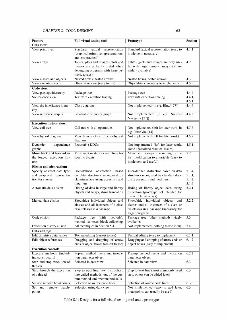
CHAPTER 8. TOOL DESIGNS 65
Feature Full visual testing tool Prototype SectionData view:View primitives Standard textual representation
(graphical primitive representationsare less practical)
Standard textual representation (easy toimplement, necessary)
4.1.1
View arrays Tables, plots and images (plots andimages are probably useful whendebugging programs with large nu-meric arrays)
Tables (plots and images are only use-ful with large numeric arrays and arewidely available)
4.2
View classes and objects Nested boxes, nested arrows Nested boxes, nested arrows 4.3View execution stack Object-like view (easy to use) Object-like view (easy to implement) 4.5.5Code view:View package hierarchy Package tree Package tree 4.4.4Source code view Text with execution tracing Text with execution tracing 4.4.1,
4.5.1View the inheritance hierar-chy
Class diagram Not implemented (in e.g. BlueJ [27]) 4.4.4
View reference graphs Browsable reference graph Not implemented (in e.g. Source-Navigator [77])
4.4.5
Execution history view:View call tree Call tree with all operations Not implemented (left for later work, in
e.g. RetroVue [14]4.5.6
View hybrid diagram View branch of call tree as hybriddiagram
Not implemented (left for later work) 4.5.9
Dynamic dependencegraphs
Browsable DDGs Not implemented (left for later work,some unresolved practical issues)
4.5.11
Move back and forward inthe logged execution his-tory
Movement in steps or searching forspecific events
Movement in steps or searching for thelast modification to a variable (easy toimplement and useful)
7.2
Elision and abstraction:Specify abstract data typeand graphical representa-tion for classes
User-defined abstraction basedon data structures recognised byclass/interface using accessors andmodifiers
User-defined abstraction based on datastructures recognised by class/interfaceusing accessors and modifiers
5.1.4,5.1.1,5.1.2,5.1.6
Automatic data elision Hiding of data in large and libraryobjects and arrays, string truncation
Hiding of library object data, stringtruncation (prototype not intended foruse with large arrays)
5.2.1
Manual data elision Show/hide individual objects andclasses and all instances of a classor all classes in a package
Show/hide individual objects andclasses and all instances of a class orall classes in a package (necessary forlarger programs)
5.2.2
Code elision Package tree (with methods),method list boxes, block collapsing
Package tree (other methods widelyavailable)
5.3
Execution history elision All techniques in Section 5.4 Not implemented (nothing to use it on) 5.4Data editing:Edit primitive data values Textual editing (easiest to use) Textual editing (easy to implement) 6.1.1Edit object references Dragging and dropping of arrow
ends or object boxes (easiest to use)Dragging and dropping of arrow ends orobject boxes (easy to implement)
6.1.2
Execution control:Execute methods (includ-ing constructors)
Pop-up method menu and invoca-tion parameter object
Pop-up method menu and invocationparameter object
6.2.2
Start and stop execution ofthreads
Selected in data view Selected in data view 6.3
Step through the executionof a thread
Step to next line, next instruction,into called methods, out of the cur-rent method and over method calls
Step to next line (most commonly usedstep, others can be added later)
6.3
Set and remove breakpoints Selection of source code lines Selection of source code lines 6.3Set and remove watch-points
Selection using data view Not implemented (easy to add later,breakpoints can usually be used)
6.3
Table 8.1: Designs for a full visual testing tool and a prototype

Chapter 9
Prototype
In order to evaluate the most important new ideas in visual testing, I have produced aprototype, which I call MVT (Matrix Visual Tester).
MVT can be divided into the following parts, each of which corresponds to a packagein the MVT package fi.hut.cs.mvt:
• Instrumentation of debuggee (fi.hut.cs.mvt.connection.instrumentation).
• Connection to debuggee (fi.hut.cs.mvt.connection).
• Data model (fi.hut.cs.mvt.data).
• View model (fi.hut.cs.mvt.view).
• User interface (fi.hut.cs.mvt.ui).
Each of these parts will be separately described in this chapter.As its name suggests, MVT is implemented using Matrix. Matrix provides MVT with a
framework for logging and visualisation of data structures. By using an existing visualiser,the time to produce the prototype visual testing tool was cut down noticeably. However,many of the execution history visualisations would have required extensive additions toMatrix.
The structure of MVT is shown in Figure 9.1.
9.1 Connection to debuggeeMVT uses the hybrid debuggee connection described in Section 7.1.5. Thus, it consists ofinstrumentation code and a runtime connection based on JPDA.
9.1.1 InstrumentationIn order to gather information effectively from the debuggee, the Java bytecode of the de-buggee is instrumented with calls to several empty dummy methods (in the MVT debug callclass fi.hut.cs.mvt.connection.instrumentation.DebugCalls) that take the infor-mation to be extracted as parameters. Calls to these methods can then be detected as methodentry events using JPDA.
The instrumentation is implemented using the class file parsing and modification facil-ities of BCEL [17]. Before starting the debuggee, the user must tell the instrumenter whichpackages or classes to instrument. The instrumenter then adds the extra method calls to thedebuggee class files.
66

CHAPTER 9. PROTOTYPE 67
Debuggee JVM
Debugger JVM
Instrumentation User program code
JDWP implementation
JDWP
Method entry events
Debug events
Commands
Commands
JDI implementation
Debug events
MVTDebuggee connection
Debug events
Data model
View model
Matrix
MVT user interface
Data change and execution events
Matrix data structure interfaces
Data
Method calls and data changes
Abstracted data structures
JDICommands
Commands
Commands
Instrumentation calls
Figure 9.1: Structure of MVT
CHAPTER 9. PROTOTYPE 68
When the instrumenter instruments a class file, it adds instrumentation code before andafter almost every bytecode instruction in the class file. Before each instruction, code isadded to copy the values read from the operand stack by the instruction and call a suitablemethod in DebugCalls to send the values to the debugger. Similarly, after the instruction,if the instruction put any new values on the stack, these values are copied and passed to amethod in DebugCalls.
The instrumenter also adds code to the start of every method to generate a unique iden-tifier for each method invocation. This is used by the data model to identify stack framesuniquely.
The instrumentation has a few minor problems that are related to the requirementsplaced by the JVM on bytecode. References to newly created objects that have not beeninitialised can only be manipulated in a limited number of ways. In particular, passing themas parameters to any method other than a constructor for the right object type is consideredan error. Due to this, newly created objects will not be visible until the first field value iswritten to them by instrumentation code or a reference to the object is stored in an object.In practice, the only effects of this limitation are that new objects are not visible until theinstrumented code actually does something with them. This may be mildly confusing, butno relevant information is lost.
Adding the instrumentation calls may cause a method to expand beyond the 64 kB limitenforced by the JVM. Methods written by human programmers are seldom large enoughto cause problems. However, some problems may be experienced with machine-generatedcode. No problems of this type were observed during testing.
9.1.2 Runtime debuggee connectionAll communication with the debuggee, including starting the JVM in which the debuggeeis run, is done using JPDA [71]. MVT uses JDI to access JPDA features.
Initially, the debuggee is started using the normal JDI procedure. In order to remove theneed to start a main method immediately, the debuggee VM is started using a dummy classwith a main method that does nothing except run into a breakpoint.
JPDA only allows one debugger-initiated method invocation to be active at a time. Ifthe debugger invokes a method through JPDA while a method invocation is active, JDIcryptically reports an unknown JDWP error of type 502 (labelled ALREADY_INVOKING inthe JDWP specification). To circumvent this problem, MVT does not invoke the methodsthe user specifies directly. Instead, it uses the thread created for the dummy main methodto start a new thread in which the user-specified method is invoked using the Java reflectionAPI (java.lang.reflect). This allows the user to invoke methods at any point in thedebuggee’s execution. Accessors are run in separate threads in a similar fashion, whichenables MVT to kill an accessor that has not finished within a suitable time limit.
MVT allows the user to step through running code a line at a time or run it to the endof a user method invocation or a breakpoint.
The debuggee connection is based on an event queue mechanism similar to that ofJPDA. The debug connection waits for events from JPDA and then processes them. Inprocessing a JPDA event, the debuggee connection may generate one or more events of itsown, which it put on its own output queue. These events are similar to the events producedby JPDA, but they are at a slightly higher level and the events produced by instrumentationcalls have been converted into a more sensible form. The data model part of MVT waits forevents from the debuggee connection part, and updates its own data model correspondingly.Whenever the user wants the debuggee to continue or step, the data model waits for andprocesses events until the criterion for interrupting execution is satisfied.
Due to namespace conflicts caused by the classes used by the instrumentation, MVTcannot be used to debug programs that use the package fi.hut.cs.mvt or any packageinside it. In practice, the only problem this causes is that MVT cannot examine itself unlessthe package names are changed in the copy that is examined.

CHAPTER 9. PROTOTYPE 69
9.2 Data modelThe data model is essentially a log of all changes made to the data structures in the program.Other aspects of the execution history, such as invoked methods, can also be considered apart of the data model. Currently, only operations that affect the data in the debuggee arelogged.
Whenever an event is received from the debuggee connection, the corresponding changesare made to the data model. MVT stores the data model in memory structures provided byMatrix (matrix.structures.memory). These structures automatically log changes andallow the user to step back and forth through the history of the data structures using theanimation controls provided by Matrix.
The data model consists of data elements (DataElement), which can be either datacontainers (DataContainer) or model variables (ModelVariable). Model variables cor-respond to individual variables in the debuggee: fields, local variables and array elements.Data containers correspond to threads (or their stacks), stack frames, objects, classes andarrays. A model variable always contains a JDI reference to a value in the debuggee. Sim-ilarly, each data container contains a reference to the corresponding thread, stack frame,object, class or array in the debuggee. Data containers also contain a number of named ele-ments. Each element is a model variable. JDI provides references to objects, classes, threadsand arrays. Stack frames are identified using a identifier generated by the instrumentationcode.
The data model is also responsible for detecting possible changes to data values ex-tracted using accessors and running the extractors to update the values. The data modelkeeps track of the extracted values. If an object is known to be mutable and updating ex-tracted values is desired for the object’s class, extracted values are updated whenever amethod call on the object exits. For most library classes (e.g. Collections), this is suffi-cient.
9.3 View modelThe view model consists of data structures that can be visualised by Matrix (they implementvarious FDT interfaces in matrix.structures.FDT) that can update themselves to reflectthe information in the data model. The top level view model object is called the nestedobject graph, which implements an extended version of the Matrix graph interface. Thenested object graph contains container arrays that correspond to the data containers in thedata model. The container arrays contain named elements that are data structures that canbe visualised by Matrix. The elements can be e.g. primitive variables, other container arraysand arrows to other container arrays.
Abstraction and elision are handled by the view model. When the view model is updatedbased on the data model, convertors are applied to transform the data into the desired form.
9.4 User interfaceThe user interface allows the user to access all the features of MVT. Most of the MVTuser interface is provided by Matrix. The MVT main window is an extended version of theMatrix prototype user interface. It contains a visualisation of the nested object graph basedon the data model, a package tree and a view of the source code of the currently runningcode.
Operations that manipulate the code of the debuggee and visualisation settings of classesand packages are performed using the package tree. To preserve screen space, the branchesof the tree corresponding to packages are collapsed by default. The class visualisation set-tings are the default settings for the instances of the class; object-specific settings override

CHAPTER 9. PROTOTYPE 70
these. If a class does not have a value for a setting, it inherits one as described in Subsec-tion 5.1.6.
The source code view shows the line at which the debuggee has stopped highlighted inthe source code.
The nested object graph shows the data in the debuggee and allows the user to manipu-late the debuggee by modifying data through drag and drop or pop-up menus.
The visualisation settings for objects include:
• Transformations for the container array view such as flipping or rotating the array aswell as turning indices and title bars on or off.
• The name of the (possibly virtual) field to show the object as.
• Whether the object is shown even though no reference to it is visible.
The class-specific default object visualisation settings include:
• Defaults for all of the object-specific settings.
• The extractors and convertors for instances of the class. The extractors and con-vertors are Java classes that implement the fi.hut.cs.mvt.data.Extractor orfi.hut.cs.mvt.data.Convertor interface. When defining the extractor or con-vertor to use for a class, String and DataContainer parameters may be specifiedto configure the extractor or convertor for use with the class.
The class-specific defaults can be saved between sessions. Object-specific settings can-not be saved.
Figure 9.2 contains a screen shot of MVT taken during the execution of the hash tabletest case (see Section 10.2). From the top down, the MVT/Matrix window in the screenshot contains:
• Menus that contain global settings and commands.
• The animator controls used to step through the logged execution history.
• The debuggee state view, containing (from left to right):
– The active thread, containing a stack frame, which contains the local variablesfor the method invocation. If several method invocations are active in a thread,they are arranged vertically in a table inside the thread box. If several threadsare active, they are all shown (unless the user changes this using elision con-trol).
– A LinearHashTable object. Both its fields (the actual table, and its size) areshown, as well as the result of passing the table to the valueOf method in theJava String class. As only the keys in the table are interesting in this context,only the key (an Integer object) is shown for each hash table entry.
– The LinearHashTable class, which contains two static fields.
• The tree of packages and classes in the class path. All packages are collapsed to savespace.
• The search method invocation described in the use case description, before it is exe-cuted using its pop-up menu.
Figure 9.3 contains a screen shot of MVT taken during the execution of the XML treetest case (see Section 10.3). The attributes and children of each XML node are shown.

CHAPTER 9. PROTOTYPE 71
Figure 9.2: MVT running the hash table test case
Figure 9.3: Part of an XML tree shown in MVT

Chapter 10
Use cases
In order to provide examples of the use of a visual testing tool and some concrete cases toevaluate the prototype against, I will present a few use cases for a visual testing tool. Thesetest cases are intended to demonstrate that a visual testing tool can be used as a debuggerto examine a wide range of programs and in addition provide a clearer data view, decreasethe need for test code and provide a better way to examine the execution history of theprogram.
The first three test cases (examining a sort routine, a hash table and a library data struc-ture) are intended to simulate different unit testing scenarios, as this type of use is partic-ularly conducive to interacting testing. Also, keeping the tests small makes the tests easierto perform. The small tests concentrate on testing the presentation of the program state,the prototype’s support for causal understanding and the generality of the prototype whenapplied to different data structures. The hash table test is also intended to test the data mod-ification and execution control aspects of the the prototype. The library data structure testshould demonstrate the prototype’s suitability for one of the most useful applications of amore abstract data view. The last test case tests the suitability of the prototype for the testingof larger programs. These four tests should provide an indication of the suitability of theprototype for software testing without requiring extensive testing that can not be performedwithin the scope of this thesis.
10.1 Debugging a sort routineDebugging a bubble sort routine is a simple test that is within the capabilities of all of thesurveyed software visualisation systems. A bubble sort routine with an off-by-one error ina loop condition is run on a small unsorted integer array and examined with a softwarevisualisation tool in order to find the bug. The sort routine is as follows (spotting the erroris left as an exercise for the reader):
public class BubbleSort {public static void sort(int[] table) {
for(int i=0;i<table.length;i++)for(int j=i+1;j<table.length-1;j++)
if (table[i]>table[j]) {int temp=table[i];table[i]=table[j];table[j]=temp;
}}
}
72

CHAPTER 10. USE CASES 73
This use case is usually easy to handle with existing graphical and visual debuggers, asthey can all display integer arrays in a meaningful fashion. In most debuggers and programvisualisers, all that has to be done is to load the program and step through it displaying thestate of the array. In order to do this with algorithm animation and simulation tools, thecode must be modified or extended to conform to the interfaces used by the tools. In Lensand Leonardo, a visualisation must be constructed.
For simple programs such as this, single stepping is quite adequate. However, beingable to step backwards through states of the program and list the executed operations mayalso be useful, as it eliminates the need for stepping through the program repeatedly.
In this case, a visual testing tool can be used much like a logging debugger such asRetroVue.
Sequence
• Run the broken sort routine on the array {4,7,3,2,5,1}, stepping through executionand viewing the array and loop indices.
• Step backwards through the execution of the program, if possible. The array andindices should be visible.
10.2 Testing a hash tableThis use case demonstrates the ability of a software visualisation tool to display structuresconsisting of objects linked with references at a suitable level of abstraction. It also providesan example of a problem that is easily detected using visual testing that is hard to find usingnormal unit testing methods.
A hash function unsuited to the data (the key modulo 10) causes hash tables that uselinear probing to become unevenly loaded and therefore inefficient. A small table is con-structed and visualised in order to find this inefficiency. The linear probing hash table im-plementation at [74] is used for this test.
When using a software visualiser with no execution control or simulation capabilities,test code must be written that creates a table and performs various operations on it. The testcode must be carefully planned to cover all different cases or edited, recompiled and rerunrepeatedly in order to provide a semblance of interactivity.
When using a debugger, the test code approach can be used. However, if the debuggersupports method invocation, interactive testing can be performed by starting the programin the debugger and then invoking the hash table implementation’s methods to construct atable and manipulate it. In all of the surveyed debuggers, this approach had some problems.BlueJ is the only debugger examined here that allows graphical method invocation; workingwith object references in the others is somewhat inconvenient. DDD and GVD can displaythe resulting structure as reasonably sensible tree of objects. With BlueJ and RetroVue, theuser has to do some digging in the object viewer to extract the keys.
The program visualisers with programmable views and the algorithm simulation andanimation tools again require additional work to produce a visualisation. However, thisvisualisation should be clearer than that produced by a debugger. An algorithm simulationtool also provides easy interactive testing.
In this case, a visual testing tool can provide the convenient interactivity and clearvisualisation of an algorithm simulation tool without the extra adaptation work.
Sequence
• Insert the keys {20,0,101,21,53,10} into the hash table.
• Step through (line by line) searching for the key 10 in the hash table.

CHAPTER 10. USE CASES 74
• Delete 10 and 0.
• Step through inserting the key 10 into the hash table.
When stepping through a search, the table entry that is being examined should be indi-cated.
10.3 Examining a data structure through a library APIThis use case is intended to demonstrate how complex library data structures written toconform to a published API can be visualised effectively.
As an example, an XML document will be loaded, parsed and accessed using theDOM API (as described in [57]) and visualised using the visual testing tool. When us-ing a debugger, the nodes in the DOM tree are shown in a very implementation-specificfashion that is very hard to work with. The children of a node can be requested using thegetChildNodes() method, which returns a NodeList that can be read using its item(intindex) method. The data can sometimes be read directly from objects referenced from thenode object, but this is implementation-specific and the fields may be empty if the parserdefers parsing until an attribute is requested (like e.g. Apache Xerces 2.3 appears to do).
Visual debuggers and visualisers that rely on visualising the data fields of an object areobviously at a disadvantage in this case, as they will show the implementation of the treenodes instead of the tree data and structure.
The programmable program visualisers and algorithm animation and simulation toolsagain require some extra code to produce the visualisation, but they can produce a veryclear view of the data.
With a visual testing tool, convertors can be combined to call the API methods andconvert the values returned by them into a meaningful visualisation. If the API is very non-intuitive, some additional convertor code may be necessary. However, the amount of codeneeded should be less than the amount required to use an algorithm simulation tool.
Sequence
• Load the Matrix default configuration file (1896 lines of XML at the time of writing)using the DOM API.
• View the tree.
10.4 Studying the behaviour of a large programThis use case is intended to evaluate the suitability of the visual testing tool for work withlarge programs. As an example, I will use jEdit [69], a Java-based text editor freely avail-able in source form. jEdit is a quite a large program (roughly 75000 lines of code). It istherefore reasonable to assume that any tool that can be successfully used to examine jEditcan also be used to examine other large programs.
Studying the static aspects of a program is seldom the most effective way to gain anunderstanding of how the program works. Running the program and trying out differentfeatures is often more educational even without a view into the internals of the program.
While manipulating a program using its normal user interface can give a good pictureof the feature set of the program, it is harder to gain an understanding of how the programworks this way. For this, some sort of view of the program execution and data is very useful.Being able to execute methods and modify data at will may help, but it is not necessary.

CHAPTER 10. USE CASES 75
Sequence
• Start jEdit.
• By examining history and/or placing breakpoints, determine how jEdit determineswhich files are loaded on startup (where this setting is stored and how).

Chapter 11
Evaluation of prototype
The prototype will be evaluated in two ways. First, a feature set comparison will be used tocompare it to the other surveyed tools. Second, the prototype will be tested against the usecases in Chapter 10.
11.1 Feature set comparisonWhen evaluating using the system defined in Table 3.1, MVT gets the results shown inTable 11.1. These results can be compared with the scores in Table 3.2. MVT was writtenwith these criteria in mind, so it is hardly surprising that it scores at least pp in every category.
11.2 Evaluation using use casesEvaluating MVT based on its feature set, as in Table 11.1, may not tell the whole story. Inorder to evaluate the performance of MVT, I have tested MVT in the use cases defined inChapter 10. The performance of MVT in these use cases should give some indication ofwhether MVT is suitable for debugging.
To put MVT’s results in perspective, the same tests will also be performed using DDDand Matrix. These two were chosen from the surveyed tools as they are freely available,can visualise Java programs, have high scores in Table 3.2 compared to similar tools andhave at least limited support for everything required by visual testing.
Like most algorithm animation/simulation tools, Matrix cannot extract informationabout the execution flow of a program (e.g. stack frames and execution position) unless theprogram explicitly maintains data structures corresponding to this information and updatesit or an extension to Matrix is written that connects to the program using instrumentation
System Gen
eral
ity
Com
plet
enes
s
Dat
am
odifi
catio
n
Exe
cutio
nco
ntro
l
Rep
rese
ntat
ion
Abs
trac
tion
Aut
omat
icvi
ewco
ntro
l
Man
ualv
iew
cont
rol
Cau
salu
nder
stan
ding
MVT ppp ppp ppp pp pp ppp pp pp pp
Table 11.1: Feature set evaluation of MVT
76
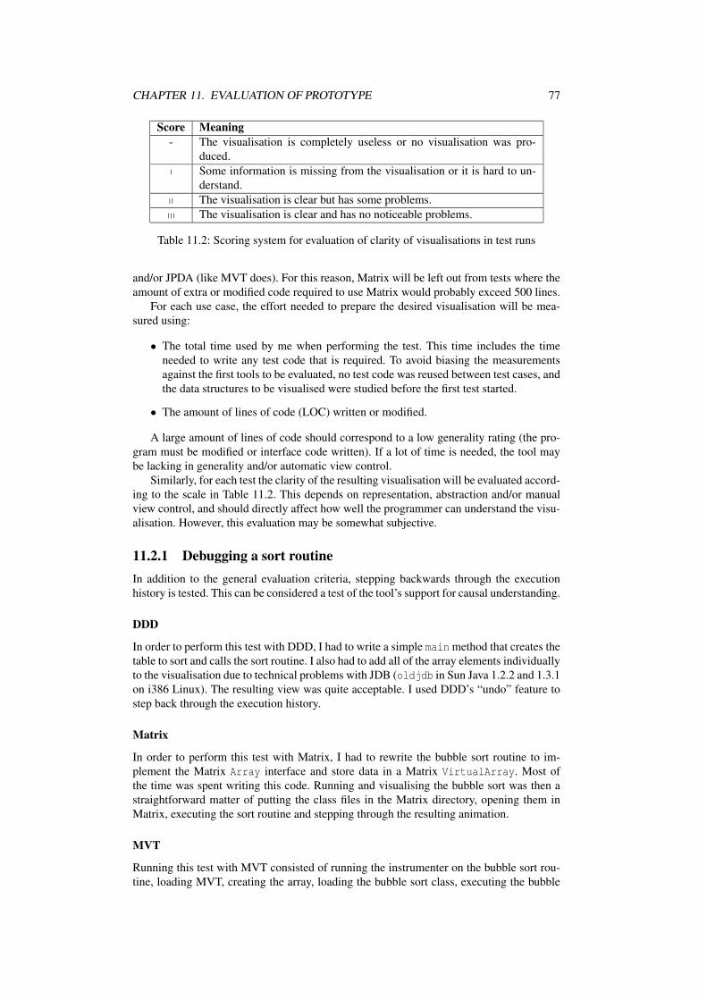
CHAPTER 11. EVALUATION OF PROTOTYPE 77
Score Meaning- The visualisation is completely useless or no visualisation was pro-
duced.p Some information is missing from the visualisation or it is hard to un-
derstand.pp The visualisation is clear but has some problems.ppp The visualisation is clear and has no noticeable problems.
Table 11.2: Scoring system for evaluation of clarity of visualisations in test runs
and/or JPDA (like MVT does). For this reason, Matrix will be left out from tests where theamount of extra or modified code required to use Matrix would probably exceed 500 lines.
For each use case, the effort needed to prepare the desired visualisation will be mea-sured using:
• The total time used by me when performing the test. This time includes the timeneeded to write any test code that is required. To avoid biasing the measurementsagainst the first tools to be evaluated, no test code was reused between test cases, andthe data structures to be visualised were studied before the first test started.
• The amount of lines of code (LOC) written or modified.
A large amount of lines of code should correspond to a low generality rating (the pro-gram must be modified or interface code written). If a lot of time is needed, the tool maybe lacking in generality and/or automatic view control.
Similarly, for each test the clarity of the resulting visualisation will be evaluated accord-ing to the scale in Table 11.2. This depends on representation, abstraction and/or manualview control, and should directly affect how well the programmer can understand the visu-alisation. However, this evaluation may be somewhat subjective.
11.2.1 Debugging a sort routineIn addition to the general evaluation criteria, stepping backwards through the executionhistory is tested. This can be considered a test of the tool’s support for causal understanding.
DDD
In order to perform this test with DDD, I had to write a simple main method that creates thetable to sort and calls the sort routine. I also had to add all of the array elements individuallyto the visualisation due to technical problems with JDB (oldjdb in Sun Java 1.2.2 and 1.3.1on i386 Linux). The resulting view was quite acceptable. I used DDD’s “undo” feature tostep back through the execution history.
Matrix
In order to perform this test with Matrix, I had to rewrite the bubble sort routine to im-plement the Matrix Array interface and store data in a Matrix VirtualArray. Most ofthe time was spent writing this code. Running and visualising the bubble sort was then astraightforward matter of putting the class files in the Matrix directory, opening them inMatrix, executing the sort routine and stepping through the resulting animation.
MVT
Running this test with MVT consisted of running the instrumenter on the bubble sort rou-tine, loading MVT, creating the array, loading the bubble sort class, executing the bubble

CHAPTER 11. EVALUATION OF PROTOTYPE 78
System Time LOC Clarity Reverse steppingDDD 10 min 6 pp YesMatrix 40 min 64 ppp YesMVT 3 min 0 ppp Yes
Table 11.3: Test results in bubble sort test
System Time LOC ClarityDDD 24 min 15 pp
Matrix 74 min 94 ppp
MVT 16 min 0 ppp
Table 11.4: Test results in hash table test
sort on the newly created array, and finally stepping through the result. No additional codewas needed.
Summary
Table 11.3 contains the test results for the bubble sort use case. Using DDD and MVTwas quick and satisfactory, while using Matrix required a disproportionate amount of extracode.
11.2.2 Testing a hash tableDDD
In order to perform this test with DDD, I had to write a simple main method that createsthe table and calls the insert, delete and search routines. I also had to add the array elementsindividually to the visualisation due to technical problems with JDB and in order to get thedesired view. The resulting view was acceptable.
Matrix
In order to perform this test with Matrix, I had to extend the hash table to implement theMatrix Array interface and modify it to store data in a Matrix VirtualArray. Most ofthe time was spent writing this code. Running and visualising the hash table was thena straightforward matter of putting the class files in the Matrix directory, opening themin Matrix, activating the test code to modify the table and stepping through the resultinganimation.
MVT
Running this test with MVT was similar to the bubble sort test; instrumentation followedby loading the class into MVT and interactively testing in MVT. No additional code wasneeded.
Summary
Table 11.4 contains the test results for the hash table use case. Using MVT was reasonablypainless, DDD required a bit more work but not too much, while Matrix required quite alot of extra test code.

CHAPTER 11. EVALUATION OF PROTOTYPE 79
System Time LOC ClarityDDD 56 min 55 p
Matrix 49 min 78 p
MVT 84 min 32 -
Table 11.5: Test results in Matrix configuration file tree test
11.2.3 Examining a data structure through a library APIIn this test, an XML tree accessed should be loaded using the DOM API and visualised asa tree. Each node in the DOM tree should be shown as a box containing the attribute typename, the attributes of the node (name and value of each attribute) and links to the childnodes. The order of the child nodes should be clearly visible.
As the purpose of this test is to examine how well MVT can be adapted to a new libraryAPI, the time used to write the extractors for XML data is included in the test.
DDD
In order to perform this test with DDD, I had to write a small program that loads the XMLfile, parses it using the DOM API and constructs a tree of simple objects containing therelevant data.
DDD failed to visualise even the converted tree properly. Apparently, DDD or oldjdbhas problems with empty arrays and arrays with more than three elements. This causedmost of the nodes of the tree to be scrambled and lack some information. This test stronglysuggests that DDD is not suitable for production use.
Matrix
The XML test code for Matrix was similar to the code used with DDD, except that theparsed tree was made available to Matrix using the Matrix Tree interface.
The resulting tree representation should have been quite clear, but rendering problems(including a large black box that covered the entire tree and the right-hand side of the treebeing cut off) made the tree hard to examine effectively.
MVT
Defining the DOM tree visualisation in MVT took roughly 40 minutes. This time mostlyconsisted of defining the abstractions for the DOM NodeList and NamedNodeMap classes(Attr objects could be directly visualised using extractors built into MVT). However, ap-plying the DOM tree visualisation to the Matrix configuration file caused MVT to spendover half an hour extracting the tree before the JDWP implementation in the debuggeecrashed. In other words, MVT produced no useful output. This indicates that MVT has se-vere performance and stability issues that make it unsuitable for use with large data struc-tures.
Both the performance problems and the crash seem to be caused by Sun’s JPDA imple-mentation. The time between requesting a method invocation and the actual execution ofthe method invocation seems to increase with every invocation. JDWP reported an internalerror before failing, which means that JDWP has a bug or insufficient error checking.
Summary
Table 11.5 contains the test results for the XML tree test. DDD and Matrix both requiredsome test code and had problems producing a graph, even though a partial result was pro-duced. MVT needed less test code, but failed to produce a graph due to implementationproblems.

CHAPTER 11. EVALUATION OF PROTOTYPE 80
System Time ClarityDDD 1 min p
Matrix 3 min pp
MVT 5 min pp
Table 11.6: Test results in MVT build file tree test
As all of the debuggers experienced technical problems, I repeated the test with asmaller XML file (a pre-release version of the build configuration file for MVT, 94 lines)in order to determine whether the problems were related to the size of the file. Table 11.6contains the results of this additional test. The time noted here is the time needed to applythe pre-defined visualisation to the new file. In this test, Matrix and MVT had no renderingproblems and produced a usable result.
11.2.4 Studying the behaviour of a large programThis test is mostly about finding things in the execution history. If the tool used providesgood support for causal understanding in practice, it is easy to find the right spot in theprogram. For these purposes, ease is considered equivalent to speed.
Using Matrix to examine the execution of a program of this type is quite unpractical, asit would require adding code to trace execution either involves instrumenting jEdit manu-ally with code that keeps track of the execution position (which involves editing thousandsof lines), writing an instrumenter that inserts the tracking code or adding a debugger con-nection to Matrix. The first option is extremely tedious, while the second and third duplicateparts of MVT.
DDD
Using DDD, I stepped through the code executed in the main jEdit class until I found thecode that loaded the list of previously opened files and opened the listed files. This wasquicker and easier than expected.
MVT
Even with only minimal extraction of data (String contents only) and instrumentation ofonly the main class (org.gjt.sp.jedit.jEdit), MVT used almost a GB of RAM evenbefore jEdit had started completely. Apparently, the main class of jEdit performs enoughoperations on its own to create a huge log. Also, each attempt to run jEdit under MVTlasted for roughly ten minutes.
The problems in this test suggest that MVT collects too much data or stores it ineffi-ciently and slows down the execution of a program badly. Thus, MVT is not suitable fortesting large programs at once. When using MVT, the user must decide on a (small) part ofa program and instrument and examine only that part.
Summary
MVT’s extensive logging makes it unsuitable for use with large programs. DDD, on theother hand, actually seems to handle this type of use case well. The test results are inTable 11.7.
11.2.5 EvaluationWhen examining a program with MVT, the user need only write extra code if he wantsto define a new type of abstraction. In this respect, MVT provides a clear advantage over

CHAPTER 11. EVALUATION OF PROTOTYPE 81
System TimeDDD 14 minMVT 75 min (failed)
Table 11.7: Test results in jEdit examination test
Matrix, as the user does not need to explicitly define every type of object to be visualised.When using DDD, the abstraction must be added to the debuggee. When using Matrix, aclass must be implemented that provides all of the visualisation.
11.3 SummaryWhile MVT has a feature set that is well suited for visual testing, it does not always workwell in practice. In particular, MVT works very badly with programs that perform lots ofoperations or create large data structures. However, getting a good visualisation at a slightlyhigher abstraction level than the implemntation level seems to be easier with MVT thanwith DDD or Matrix. This means that visual testing, even in this crude implementation,appears to simplify the testing of small chunks of code. In other words, MVT seems tobe quite a decent tool for unit testing. MVT can also be used to generate visualisations ofsmall programs quickly.
MVT has several performance-related problems that must be resolved in order to pro-duce a good visual testing tool. In particular, more efficient ways to extract informationfrom a debuggee and store the execution history are clearly needed.
Chapter 12
Conclusion
The goal of visual testing (outlined in Chapter 2) is to make it easier for programmers totest and debug their code. Visual testing does this by combining ideas from different typesof software visualisation into a single tool that should make it easier for a programmerto try out different operations on program code and examine the results visually. I haveevaluated several software visualisation tools in Chapter 3. All of these systems providesome features that could be useful in visual testing, but none of them is an effective visualtesting tool.
Together, the surveyed software visualisation tools have almost everything that is neededfor a visual testing tool. For this reason, I have examined and evaluated relevant visuali-sation (Chapter 4), elision and abstraction (Chapter 5) and debuggee control (Chapter 6)techniques. Most of these techniques can be found in the surveyed tools.
Using these evaluations, I have found ways to present the state and execution historyof a program effectively. Most of the state of a program can be shown in a data viewthat primarily consists of objects (shown as boxes with data fields) that may contain orrefer (through arrows originating in a data field) to each other. By augmenting the objectdisplay with boxes for classes and threads and adding a simple display of source codewith highlighting of the current statement, the data view can display most of the state ofthe program. For clarity, data should be shown at a level of abstraction close to the levelused by the programmer when writing his code. Making use of the abstraction inherent inobject-oriented code seems to be an effective way to provide data abstraction in a debugger.Many ways to show the execution history of a program exist, but the best ways seem tobe allowing the user to step through the states of his program and showing the executedoperations as a tree or in the data view as a hybrid diagram.
In order to efficiently test software, the user should be allowed to specify, with a mini-mum of fuss, the operations he wants the software to perform. Allowing the user to graph-ically manipulate the data in his program and invoke methods at will provides additionalflexibility and eliminates much of the need for test code.
Most of the aforementioned techniques have been used earlier, but they have not beencombined. A visual testing tool consists almost entirely of software visualisation and de-bugging techniques that have been developed earlier and some additional ideas to makethese different techniques work together.
After examining different approaches to the implementation of a visual testing toolin Chapter 7, I have presented (in Chapter 8) designs for a full visual testing tool and aprototype visual testing tool that demonstrates the feasibility of the visual testing conceptand the new techniques applied in it.
Even though my tests (Chapter 11) show that the prototype visual testing tool has severeperformance issues, my tests suggest that it is a useful tool for unit testing. As unit testingis one of the intended uses for a visual testing tool, this means that the prototype alreadygoes some way towards the goals of visual testing.
82

CHAPTER 12. CONCLUSION 83
MVT was put together in two man-months and contains only crude implementations ofa few of the ideas of visual testing. Despite this, my tests suggest that it is an improvementover existing tools in tasks such as unit testing and debugging. This suggests that a wellimplemented complete visual testing tool can prove to be a powerful tool.
12.1 Future researchThere are several matters that need to researched in more depth before a proper visualtesting tool can be produced:
• The execution history logs produced by MVT are far too large. Ways must be foundto rid these logs of irrelevant and redundant information and store the remaininginformation efficiently.
• Some issues remain unsolved in adapting dependence graphs for use in visualisation.
• A more efficient way to extract information from a running program and control it isneeded. In the long term, the best solution is probably to adapt a virtual machine tovisual testing.
• The user interface of the visual testing tool needs to be planned more carefully thanMVT was. In particular, common operations should be made easier to perform.
• The possibility of adding some sort of automatic checking of the validity of the pro-gram (such as assertions) combined with some sort of visible warnings in the visualtesting tool should be investigated.
• The possibilities of adapting visual testing to languages other than Java should beinvestigated.
If the above matters are researched, it may be possible to produce a visual testing toolthat is truly a useful aid in debugging and testing real-world software.

Bibliography
[1] Hiralal Agrawal, Richard A. DeMillo and Eugene H. Spafford. Dynamic slicing inthe presence of unconstrained pointers. In Symposium on Testing, Analysis, andVerification, pages 60–73, 1991.
[2] Hiralal Agrawal and Joseph R. Horgan. Dynamic program slicing. ACM SIGPLANNotices, volume 25, number 6, pages 246–256, June 1990.
[3] Tankut Akgul and Vincent J. Mooney, III. Instruction-level reverse execution fordebugging. Technical Report GIT-CC-02-49, Georgia Institute of Technology, 2002.
[4] Andrew W. Appel. Modern Compiler Implementation in Java. CambridgeUniversity Press, 1998.
[5] Ricardo Baeza-Yates, Gastón Quezada and Gastón Valmadre. Visual debugging andautomatic animation of C programs. In Peter D. Eades and Kang Zhang, editors,Software Visualisation, volume 7, pages 46–58. World Scientific, Singapore, 1996.
[6] Ryan S. Baker, Michael Boilen, Michael T. Goodrich, Roberto Tamassia andB. Aaron Stibel. Testers and visualizers for teaching data structures. In Theproceedings of the thirtieth SIGCSE technical symposium on Computer scienceeducation, pages 261–265. ACM Press, 1999.
[7] Thomas A. Ball and Stephen G. Eick. Software visualization in the large. IEEEComputer, volume 29, number 4, pages 33–43, April 1996.
[8] John L. Bentley and Brian W. Kernighan. A system for algorithm animation.Computing Systems, volume 4, number 1, pages 5–30, 1991.
[9] Michael R. Birch, Christopher M. Boroni, Frances W. Goosey, Samuel D. Patton,David K. Poole, Craig M. Pratt and Rockford J. Ross. DYNALAB — A dynamiccomputer science laboratory infrastructure featuring program animation. InProceedings of the Twenty-Sixth SIGCSE Technical Syposium on Computer ScienceEducation, pages 29–33, March 1995.
[10] Marc H. Brown. Exploring algorithms using Balsa-II. Computer, volume 21,number 5, pages 14–36, May 1988.
[11] Marc H. Brown. Zeus: a system for algorithm animation and multi-view editing. InProceedings of 1991 IEEE Workshop on Visual Languages, pages 4–9, Kobe, Japan.IEEE, October 1991.
[12] Marc H. Brown, Marc A. Najork and Roope Raisamo. A Java-based implementationof collaborative active textbooks. In 1997 IEEE Symposium on Visual Languages,pages 372–379, September 1997.
[13] Marc H. Brown and Robert Sedgewick. A system for algorithm animation. InProceedings of the 11th annual conference on Computer graphics and interactivetechniques, pages 177–186. ACM Press, 1984.
84

BIBLIOGRAPHY 85
[14] John Callaway. Visualization of threads in a running Java program. Master’s thesis,University of California, June 2002.
[15] Jonathan J. Cook. Reverse execution of Java bytecode. The Computer Journal,volume 45, number 6, pages 608–619, 2002.
[16] Pierluigi Crescenzi, Camil Demetrescu, Irene Finocchi and Rossella Petreschi.Reversible execution and visualization of programs with LEONARDO. Journal ofVisual Languages and Computing, volume 11, number 2, pages 125–150, 2000.
[17] Markus Dahm. Byte code engineering with the BCEL API. Technical ReportB-17-98, Institut für Informatik, Freie Universität Berlin, April 2001.
[18] Matthew B. Dwyer, James C. Corbett, John Hatcliff, Stefan Sokolowski andHongjun Zheng. Slicing multi-threaded Java programs: A case study. TechnicalReport SU CIS TR 99-7, Kansas State University, 1999.
[19] Jeanne Ferrante, Karl J. Ottenstein and Joe D. Warren. The program dependencegraph and its use in optimization. ACM Transactions on Programming Languagesand Systems (TOPLAS), volume 9, number 3, pages 319–349, July 1987.
[20] Martin Fowler and Kendall Scott. UML distilled: a brief guide to the standard objectmodeling language. Addison-Wesley, Second edition, 2000.
[21] James Gosling, Bill Joy, Guy Steele and Gilad Bracha. The Java LanguageSpecification. Addison-Wesley, Second edition, June 2000.
[22] Jyrki Haajanen, Mikael Pesonius, Erkki Sutinen, Jorma Tarhio, Tommi Teräsvirtaand Pekka Vanninen. Animation of user algorithms on the Web. In Proceedings ofIEEE Symposium on Visual Languages, pages 360–367. IEEE, 1997.
[23] Robert R. Henry, Kenneth M. Whaley and Bruce Forstall. The University ofWashington illustrating compiler. In Proceedings of the ACM SIGPLAN 1990conference on Programming language design and implementation, pages 223–233.ACM Press, 1990.
[24] Christopher D. Hundhausen. A meta-study of software visualization effectiveness.Journal of Visual Languages and Computing, volume 13, number 3, pages 259–290,2002.
[25] Bertrand Ibrahim. World-wide algorithm animation. In Conference Proceedings ofthe First World-Wide-Web conference, pages 305–316, May 1994.
[26] Xiaoping Jia. Object-oriented Software Development Using Java. Addison-Wesley,June 2000.
[27] Michael Kölling, Bruce Quig, Andrew Patterson and John Rosenberg. The BlueJsystem and its pedagogy. Journal of Computer Science Education, Special Issue onLearning and Teaching Object Technology, volume 13, number 4, December 2003.
[28] Ari Korhonen. World Wide Web (WWW) tietorakenteiden ja algoritmientietokoneavusteisessa opetuksessa. Master’s thesis, Helsinki University ofTechnology, May 1997.
[29] Ari Korhonen. Algorithm Animation and Simulation. Licentiate’s thesis, HelsinkiUniversity of Technology, May 2000.
[30] Ari Korhonen. Visual Algorithm Simulation. Doctoral thesis, Helsinki University ofTechnology, 2003.

BIBLIOGRAPHY 86
[31] Ari Korhonen and Lauri Malmi. Matrix — Concept animation and algorithmsimulation system. In Proceedings of the Working Conference on Advanced VisualInterfaces - AVI 2002, pages 109–114. ACM, 2002.
[32] James F. Korsh, Paul S. LaFollette, Jr. and Raghvinder Sangwan. Animating studentsand programs in the laboratory. In Proceedings of 1998 Frontiers in EducationConference, Tempe, Arizona. ASEE and IEEE, November 1998.
[33] Paul S. LaFollette, Jr., James F. Korsh and Raghvinder S. Sangwan. A visualinterface for effortless animation of C/C++ programs. Journal of Visual Languages& Computing, volume 11, number 1, pages 27–48, February 2000.
[34] Craig Larman. Applying UML to Patterns. Prentice-Hall, Second edition, 2002.
[35] Bil Lewis. Debugging backwards in time. In Michiel Ronsse, editor, Proceedings ofthe Fifth International Workshop on Automated Debugging, Ghent, Belgium.September 2003.
[36] Tim Lindholm and Frank Yellin. The Java Virtual Machine Specification.Addison-Wesley, Second edition, April 1999.
[37] Sougata Mukherjea and John T. Stasko. Applying algorithm animation techniquesfor program tracing, debugging, and understanding. In Proceedings of the 15thinternational conference on Software Engineering, pages 456–465. IEEE ComputerSociety Press, 1993.
[38] Sougata Mukherjea and John T. Stasko. Toward visual debugging: integratingalgorithm animation capabilities within a source-level debugger. ACM Transactionson Computer-Human Interaction (TOCHI), volume 1, number 3, pages 215–244,1994.
[39] Brad A. Myers, Ravinder Chandhok and Atul Sareen. Automatic data visualizationfor novice Pascal programmers. In Proceedings of IEEE Workshop on VisualLanguages, pages 192–198, Pittsburgh, Pennsylvania, USA. October 1988.
[40] James Noble, Lindsay Groves and Robert Biddle. Object oriented programvisualisation in Tarraingím. Technical Report CS-TR-95/15, Victoria University ofWellington, September 1995.
[41] Unified Modeling Language (UML), version 1.5. Object Management Group, 2003.
[42] John O’Connor and Edmund Robertson. The Arabic numeral system. In TheMacTutor History of Mathematics archive. University of St Andrews, January 2001.
[43] Rainer Oechsle and Thomas Schmitt. Javavis: Automatic program visualization withobject and sequence diagrams using the Java Debug Interface (JDI). In S. Diehl,editor, Software Visualization, pages 176–190, Dagstuhl Castle, Germany.Springer-Verlag, 2002.
[44] Willard C. Pierson and Susan H. Rodger. Web-based animation of data structuresusing JAWAA. In Twenty-ninth SIGCSE Technical Symposium on Computer ScienceEducation, pages 267–271, 1998.
[45] Alex Potanin and James Noble. Checking ownership and confinement properties.Technical Report CS-TR-02/6, Victoria University of Wellington, June 2002.
[46] Blaine A. Price, Ronald M. Baecker and Ian S. Small. A principled taxonomy ofsoftware visualization. Journal of Visual Languages and Computing, volume 4,number 3, pages 211–266, 1993.

BIBLIOGRAPHY 87
[47] Richard Rasala. Automatic array algorithm animation in C++. In The proceedings ofthe thirtieth SIGCSE technical symposium on Computer science education, pages257–260. ACM Press, 1999.
[48] Gruia-Catalin Roman, Kenneth C. Cox, C. Donald Wilcox and Jerome Y. Plun.Pavane: A system for declarative visualization of concurrent computations. Journalof Visual Languages and Computing, volume 3, number 2, pages 161–193, June1992.
[49] RTI. The economic impacts of inadequate infrastructure for software testing.Planning report 02-3, NIST, May 2002.
[50] Raghvinder S. Sangwan, James F. Korsh and Paul S. LaFollette, Jr. A system forprogram visualization in the classroom. In Proceedings of the twenty-ninth SIGCSEtechnical symposium on Computer science education, pages 272–276, Atlanta,Georgia, USA. ACM, ACM Press, New York, New York, USA, 1998.
[51] Saurabh Sinha and Mary Jean Harrold. Control-flow analysis of programs withexception-handling constructs. Technical Report OSU-CISRC-7/98-TR25, OhioState University, July 1998.
[52] John T. Stasko. Tango: A framework and system for algorithm animation.Computer, volume 23, number 9, pages 27–39, September 1990.
[53] John T. Stasko. Using student-built algorithm animations as learning aids. InProceedings of the ACM Technical Symposium on Computer Science Education,pages 25–29, San Jose, California, USA. February 1997.
[54] John T. Stasko and Eileen Kraemer. A methodology for building application-specificvisualizations of parallel programs. Journal of Parallel and Distributed Computing,volume 18, number 2, pages 258–264, June 1993.
[55] Thomas G. Stockham and Jack B. Dennis. FLIT — Flexowriter Interrogation Tape:A symbolic utility program for the TX-0. Memo 5001-23, MIT, July 1960.
[56] Inner Classes Specification. Sun Microsystems, February 1997.
[57] Java 2 Platform, Standard Edition, v 1.4.1 API Specification. Sun Microsystems,2002.
[58] Erkki Sutinen, Jorma Tarhio, Simo-Pekka Lahtinen, Antti-Pekka Tuovinen, ErkkiRautama and Veijo Meisalo. Eliot — An algorithm animation environment.Technical Report A-1997-4, Department of Computer Science, University ofHelsinki, Finland, November 1997.
[59] Fumiaki Umemori, Kenji Konda, Reishi Yokomori and Katsuro Inoue. Design andimplementation of bytecode-based Java slicing system. Technical Report 407, OsakaUniversity, December 2002.
[60] Mark Weiser. Programmers use slices when debugging. Communications of theACM, volume 25, number 7, pages 446–452, July 1982.
[61] Steven J. Zeil. AlgAE (Algorithm Animation Engine) Programmers’ Manual. OldDominion University, March 2001.
[62] Andreas Zeller. Datenstrukturen visualisieren und animieren mit DDD. In Proc.GI-Workshop: Softwarevisualisierung (SV 2000), Schloß Dagstuhl. May 2000.
[63] Andreas Zeller. Debugging with DDD. Universität Passau, First (for DDD version3.2) edition, January 2000.

BIBLIOGRAPHY 88
[64] Jianjun Zhao. Dynamic slicing of object-oriented programs. In Technical ReportSE-98-119, pages 17–23. Information Processing Society of Japan, May 1998.
[65] Peter Brummund and Ngozi V. Uti. Complete Collection of Algorithm Animations.WWW site at http://www.cs.hope.edu/~alganim/ccaa/, June 2001. Checkedon 2nd October 2003.
[66] Nathan Fiedler. JSwat — Graphical Java debugger. WWW site athttp://www.bluemarsh.com/java/jswat/, 2003. Checked on 2nd October 2003.
[67] The GNU Visual Debugger. WWW site at http://libre.act-europe.fr/gvd/,July 2003. Checked on 2nd October 2003.
[68] Javix visual debugger. WWW site at http://www.javix.com/, 2000. Checked on2nd October 2003.
[69] jEdit. WWW site at http://www.jedit.org/, September 2003. Checked on 2ndOctober 2003.
[70] JIVE. WWW site at http://jive.dia.unisa.it/, 2003. Checked on 2ndOctober 2003.
[71] Java Platform Debugger Architecture. WWW site athttp://java.sun.com/j2se/1.4.1/docs/guide/jpda/, 2002. Checked on 2ndOctober 2003.
[72] Chuck McManis. A first look at Borland’s JBuilder IDE. WWW page athttp://www.javaworld.com/javaworld/jw-11-1997/jw-11-indepth.html,2003. Checked on 2nd October 2003.
[73] Prosasim. WWW site at http://www.prosa.fi/eng/pr2Sim.htm. Checked on2nd October 2003.
[74] Graham Roberts. Simple linear probing hash table class. WWW page athttp://www.cs.ucl.ac.uk/staff/G.Roberts/1b11/classlinearhashtable.html,March 2002. Checked on 2nd October 2003.
[75] Johannes Sixt. KDbg — A graphical debugger interface. WWW site athttp://members.nextra.at/johsixt/kdbg.html, September 2003. Checked on2nd October 2003.
[76] Skillmarket — A daily look at in-demand tech skills. WWW site athttp://mshiltonj.com/sm/, October 2003. Checked on 2nd October 2003.
[77] Source-Navigator. WWW page at http://sourcenav.sourceforge.net/, June2003. Checked on 2nd October 2003.
[78] Tango/04 visual debugger. WWW site athttp://www.tango04.com/products/vdw/, 2003. Checked on 2nd October 2003.
[79] TIOBE programming community index. WWW site athttp://www.tiobe.com/tpci.htm, October 2003. Checked on 2nd October 2003.
[80] Introduction to the VC++.NET debugger. WWW page athttp://csciwww.etsu.edu/blair/Using_Debugger.htm, August 2002.Checked on 2nd October 2003.
[81] Visicomp. WWW site at http://www.visicomp.com/, 2002. Checked on 2ndOctober 2003.