Visual Analysis of Urban Environment

HAL Id: halshs-02472303https://halshs.archives-ouvertes.fr/halshs-02472303

Submitted on 10 Feb 2020

HAL is a multi-disciplinary open accessarchive for the deposit and dissemination of sci-entific research documents, whether they are pub-lished or not. The documents may come fromteaching and research institutions in France orabroad, or from public or private research centers.

L’archive ouverte pluridisciplinaire HAL, estdestinée au dépôt et à la diffusion de documentsscientifiques de niveau recherche, publiés ou non,émanant des établissements d’enseignement et derecherche français ou étrangers, des laboratoirespublics ou privés.

Visual Analysis of Urban EnvironmentFrançois Sarradin, Daniel Siret, Gérard Hégron

To cite this version:François Sarradin, Daniel Siret, Gérard Hégron. Visual Analysis of Urban Environment. First In-ternational Workshop on Architectural and Urban Ambient Environment, Feb 2002, Nantes, France.�halshs-02472303�

https://halshs.archives-ouvertes.fr/halshs-02472303

https://hal.archives-ouvertes.fr

First International Workshop on Architectural and Urban Ambient Environment; Nantes February 6–8, 2002

Visual Analysis of Urban EnvironmentFrançois Sarradin — Daniel Siret — Gérard Hégron

Laboratoire CERMA – École d’Architecture de NantesRue Massenet – BP 81 93144 319 NANTES CEDEX 3

{sarradin,siret,hegron}@cerma.archi.fr

1. IntroductionThis paper presents a survey of methods used to model and to analyse visual events in urbanscenes. What we call a visual event is an event which occurs in the visual field while we aremoving or while the scene is moving. This could be an object appearance or disappearance, ora shape, a colour, or a texture modification. But here, we mainly consider the visual eventsprovided by objects set during a motion.

In the second section, we examine some methods to model the events that come insideour visual field, giving a first interpretation to a urban environment. This is done aftershowing methods to represent the visual field. In the third section, we focus on differentmethods used to analyse and to evaluate the visibility in urban environment. Finally, weconclude on the way each of these representations of visual perceptions and each of thesevisual analysis methods act, and in which way they could be extended.

2. Visual event representationRepresentation of urban scenes can be made by symbolizing buildings, streets, places, etc. Wecan also add the visual events which appear as observers move in the streets. The visualevents generate transitions in the observer visual field like appearance and disappearance ofobjects, colour changing, shape transformation, etc. They provide important informationabout the visual effects.

The purpose of this section is about the representation of visual events. First, we show2D motionless projections of the visual field which can be used in this representation. Second,we present the visual event sequences acting by motion decomposition into pictures. Apartfrom all projection, Lynch and Thiel proposed a notation to describe the visual perception ofspace and motion, and the orientation sense. Then, we show 2D and 3D methods to determinevisual events and regions where visual informations do not change.

2.1. 2D projections of the visual fieldHere, we study the visual field representations in a motionlessness context. Most of theserepresentations use a geometrical projection in order to imitate what we see or how we recordour visual world.

2.1.1. Perspective projectionThe perspective projection study began with italian painters from Renaissance. They wishedto create an illusion: their goal was to show objects in three dimensions inside their paintings.It is used in architecture or in image synthesis in order to give a realistic representation. It isalso used in simulation for architectural and urban project in order to determine the sunlighting time or the incident energy from the sky [Groleau, 2002].

According to Panofsky, the perspective projection is “the aptitude to represent several


objects with the part of the space in which they are, so that the concept of material support ofthe picture is completely driven out by the concept of transparent plan, so that we believe, ourglance crosses to plunge into an imaginary external space which would contain all theseobjects into an apparent succession and which would not be limited but only cut out by theedges of the picture” [Panofsky, 1975].

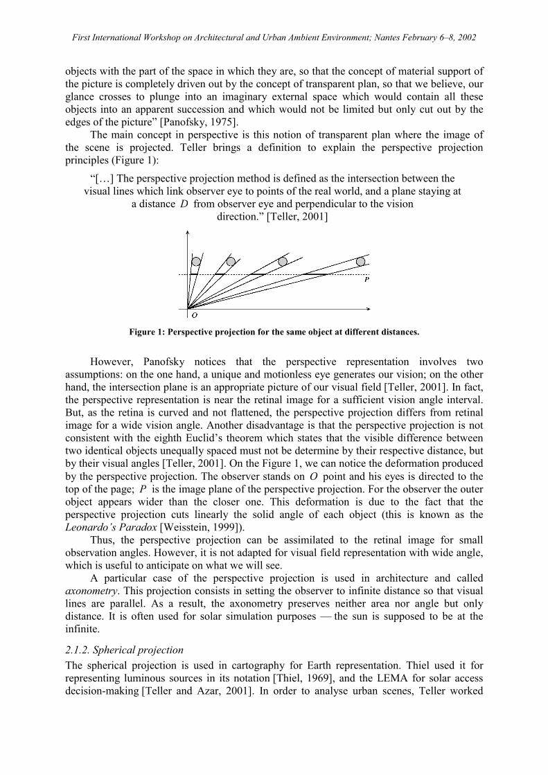
The main concept in perspective is this notion of transparent plan where the image ofthe scene is projected. Teller brings a definition to explain the perspective projectionprinciples (Figure 1):

“[…] The perspective projection method is defined as the intersection between thevisual lines which link observer eye to points of the real world, and a plane staying at

a distance D from observer eye and perpendicular to the visiondirection.” [Teller, 2001]

Figure 1: Perspective projection for the same object at different distances.

However, Panofsky notices that the perspective representation involves twoassumptions: on the one hand, a unique and motionless eye generates our vision; on the otherhand, the intersection plane is an appropriate picture of our visual field [Teller, 2001]. In fact,the perspective representation is near the retinal image for a sufficient vision angle interval.But, as the retina is curved and not flattened, the perspective projection differs from retinalimage for a wide vision angle. Another disadvantage is that the perspective projection is notconsistent with the eighth Euclid’s theorem which states that the visible difference betweentwo identical objects unequally spaced must not be determine by their respective distance, butby their visual angles [Teller, 2001]. On the Figure 1, we can notice the deformation producedby the perspective projection. The observer stands on O point and his eyes is directed to thetop of the page; P is the image plane of the perspective projection. For the observer the outerobject appears wider than the closer one. This deformation is due to the fact that theperspective projection cuts linearly the solid angle of each object (this is known as theLeonardo’s Paradox [Weisstein, 1999]).

Thus, the perspective projection can be assimilated to the retinal image for smallobservation angles. However, it is not adapted for visual field representation with wide angle,which is useful to anticipate on what we will see.

A particular case of the perspective projection is used in architecture and calledaxonometry. This projection consists in setting the observer to infinite distance so that visuallines are parallel. As a result, the axonometry preserves neither area nor angle but onlydistance. It is often used for solar simulation purposes — the sun is supposed to be at theinfinite.

2.1.2. Spherical projectionThe spherical projection is used in cartography for Earth representation. Thiel used it forrepresenting luminous sources in its notation [Thiel, 1969], and the LEMA for solar accessdecision-making [Teller and Azar, 2001]. In order to analyse urban scenes, Teller worked


with three kinds of spherical projections.The spherical projection can be defined as the intersection between visual lines, which

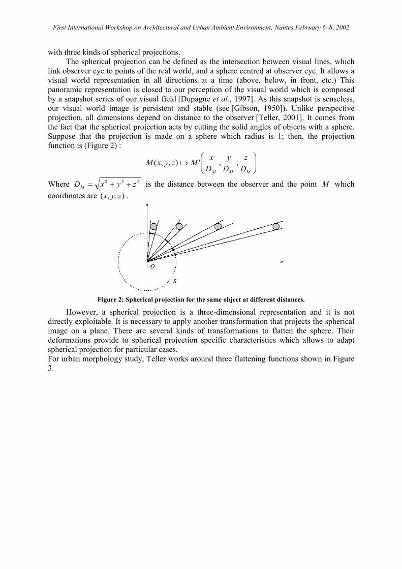
link observer eye to points of the real world, and a sphere centred at observer eye. It allows avisual world representation in all directions at a time (above, below, in front, etc.) Thispanoramic representation is closed to our perception of the visual world which is composedby a snapshot series of our visual field [Dupagne et al., 1997]. As this snapshot is senseless,our visual world image is persistent and stable (see [Gibson, 1950]). Unlike perspectiveprojection, all dimensions depend on distance to the observer [Teller, 2001]. It comes fromthe fact that the spherical projection acts by cutting the solid angles of objects with a sphere.Suppose that the projection is made on a sphere which radius is 1; then, the projectionfunction is (Figure 2) :

��

��

�

MMM Dz

Dy

DxMzyxM ,,'),,( �

Where 222 zyxDM �� is the distance between the observer and the point M whichcoordinates are ),,( zyx .

Figure 2: Spherical projection for the same object at different distances.

However, a spherical projection is a three-dimensional representation and it is notdirectly exploitable. It is necessary to apply another transformation that projects the sphericalimage on a plane. There are several kinds of transformations to flatten the sphere. Theirdeformations provide to spherical projection specific characteristics which allows to adaptspherical projection for particular cases.For urban morphology study, Teller works around three flattening functions shown in Figure3.


Figure 3: Three transformations to flatten a sphere [Teller, 2001]: (a) stereographic projection, (b)orthogonal projection, (c) isoaire projection.

� Stereographic projection (Figure 4). The stereographic projection is a “map projectionin which great circles are circles and loxodromes1 are logarithmic spirals” [Weisstein,1999]. Its main property is to conserve tangential angles. According to Teller, thestereographic projection preserves visual aspect of 3D shapes rather well [Teller,2001]. The flattening function is given below [Teller and Azar, 2001]:

��

��

�

�� zy

zxzyx

1,

1),,( �

Figure 4: Stereographic projection in Liège (right: place Xavier-Neujean [Teller, 2001],left: Cité administrative [Dupagne et al., 1997]).

� Orthogonal projection. The orthogonal projection preserves the vertical angles. Thus,the radial distances inside the projection is proportional to the observable height.However, it does not preserve neither area nor angle. The equidistant projection isuseful to compare the visual height. Its flattening function acts by a substitution of theheight [Teller and Azar, 2001]:

),(),,( yxzyx �

� Isoaire projection. With the isoaire projection, the surfaces projected on the image arerepresentative of the solid angles intercepted on the sphere. The flattening function isgiven below [Teller and Azar, 2001]:

1 “The loxodrome is the path taken when a compass is kept pointing in a constant direction” [Weisstein, 1999].


��

�

�

��

�

�

�

�

�

�2222

1,1),,(yxzy

yxzxzyx �

The spherical projection is an interesting representation of the visual world as it isrelatively consistent with our representation. Although it can not be exploited directly, a mapprojection (i.e. stereographic projection, equidistant projection, isoaire projection) applied tothe spherical projection produces deformations which highlight scene characteristics likeheight ratio, area shape ratio or angle ratio. From a certain viewpoint, the spherical projectionis adaptable. However, it presupposes that we have a unique eye, and, as it is a projection on asurface, the deepness ratio between objects disappears. The projection of a small and nearobject can be as important as a bigger but farther one.

We will show in section 3.3 a use of spherical projection in visual analysis of urbanscenes by processing sky opening generated by the building shapes.

2.2. Visual event sequencesA sequence is a series of more or less realistic images ordered in time, which is obtainedduring a motion (i.e. motion of the visual field, or motion of an object in the visual field). Inorder to decompose movement into image series, Eadweard Muybridge generated severalphotographic sequences, between 1884 and 1885, with an apparatus composed of severalcameras linearly disposed. This strange apparatus was able to decompose human or animalmotions (e.g. walking, running, jumping, etc.) Then, the Lumière’s brothers created theCinématographe in 1894. Its principle was to decompose movement into image sequences.

Much later, some urban designers have argued that movement can be read andunderstood as a pictorial sequence. Namely, Cullen talked about the approach of architecturalobjects by using pictorial sequences [Cullen, 1961]. Appleyard, Lynch et al. tried differenttechniques to record visual sequences in order to analyse it [Appleyard et al., 1964]. One ofthem consists in using the motion pictures which record sequences in a permanent form thatcan be shown to large groups of people. However, they did not keep this technique because of“the inherent difference between the camera and the human eye” [Appleyard et al., 1964].Later, Bosselmann tried to represent a walk through Venice by using a sequence of drawingswith a text explaining what he saw plus additional informations [Bosselmann, 1998].However, the author noticed some disadvantages to this technique. For example, the glancedirection in the drawings follows the observer motion direction. Besides, there are no drawingrepresenting the view to the right, to the left, at rear, etc. Thus, no drawing could represent theview which opens on each side of the observer when he is on a bridge forexample [Bosselmann, 1998].

In this section, we will focus on a method, proposed by Panerai, based on pictorialsequences, which record the visual effects.

Sequential analysisIn order to record the motion, the movie cameras decompose it into a series of image. Paneraireused this idea of visual sequence and adapted it to represent visual events on urbanroutes [Panerai, 1970][Panerai et al., 1997, 1999]. Inspired by de Wolfe [de Wolfe, 1963], thismethod proceeds by isolating and identifying in a sequence different pictures which refer to acodified and schematic configuration of the scene. These pictures can be named [Panerai etal., 1999]:

� Picture illustrating general viewpoints: symmetry or dissymmetry; lateral demarcationor axial demarcation; opening or closure; convexity or concavity.

� Pictures insisting on lateral walls: horizontal or vertical cutting up, undulation; face


relation; deference, indifference, or competition.

� Pictures studying lateral walls extension to vanish point and beyond: narrowing,strangling, or wings effect; open or hidden highlighting; deflection; demarcation.

� Pictures characterizing the front closure of the visual field: centring or diaphragm.

Figure 5: Examples of picturesque elements [Panerai et al., 1999]: symmetry (1a), opening (3a),convexity (4a).

A sequence is composed of a particular picture suite configuration that can be called alinkage2. A picturesque scene results in accumulation in short distances of breaks in the logicof the linkage. For monumental effects, the sequence consists of relatively slow successionswith superpositions of pictures.

In order to complete sequential analysis, it is necessary to collect pictures and linkagesin order to get set of linkages and to process entire sequences. A first solution consists inassembling pictures linked to an object. In this case, landmarks and monuments play aprimary role and sequences are generated by these objects. A second solution consists inassembling pictures by theme, then to introduce the cuts when the theme changes; a sign or amark allows sometimes to determine a cut.

The sequential analysis method was tested by Dupagne and Teller, with picturesproduced by stereographic projection, in order to study routes in open spaces [Dupagne et al.,1997] (see section 2.1). Following their point of view, it is not really a tool for decision-making. They describe it as a basic tool to serve in reflection or in presentation of projectintents.

2.3. Visual event notation

2.3.1. The view from the roadAs we walk in the street or drive on the road, we see all kind of visual informations whichreveal our motion. They are based on our knowledge of architectural objects. In the UnitedStates, during 1950s, it is possible to drive on expressways through the cities at acceleratedspeed. On these quick axis, the visual informations are numerous and stream quickly. Inanswer to the confusion that could be generated by this evolution, Appleyard, Lynch andMyer have created a notation in a view to provide an ‘artistic’ sense for highway because:“road-watching is a delight, and the highway is — or at least might be — a work ofart” [Appleyard et al., 1964]. Their notation is based on notation used by Lynch in [Thiel,1969] and by Thiel.

Two components are considered: the space and the motion sensations on the one hand,the observer orientation on the other hand. For the first one, Appleyard, Lynch and Myer haveclassified the visual informations relative to the motion type they involve [Appleyard et al.,1964]. The motion sensation includes the apparent self-motion generated by the road (e.g.

2 Panerai uses the french term enchaînement that could to be translated into the term ‘linkage’ used for cinema.


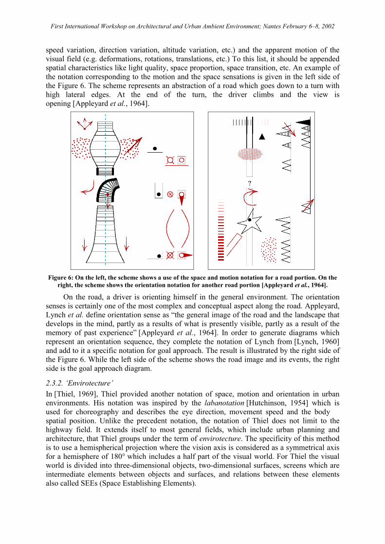
speed variation, direction variation, altitude variation, etc.) and the apparent motion of thevisual field (e.g. deformations, rotations, translations, etc.) To this list, it should be appendedspatial characteristics like light quality, space proportion, space transition, etc. An example ofthe notation corresponding to the motion and the space sensations is given in the left side ofthe Figure 6. The scheme represents an abstraction of a road which goes down to a turn withhigh lateral edges. At the end of the turn, the driver climbs and the view isopening [Appleyard et al., 1964].

Figure 6: On the left, the scheme shows a use of the space and motion notation for a road portion. On theright, the scheme shows the orientation notation for another road portion [Appleyard et al., 1964].

On the road, a driver is orienting himself in the general environment. The orientationsenses is certainly one of the most complex and conceptual aspect along the road. Appleyard,Lynch et al. define orientation sense as “the general image of the road and the landscape thatdevelops in the mind, partly as a results of what is presently visible, partly as a result of thememory of past experience” [Appleyard et al., 1964]. In order to generate diagrams whichrepresent an orientation sequence, they complete the notation of Lynch from [Lynch, 1960]and add to it a specific notation for goal approach. The result is illustrated by the right side ofthe Figure 6. While the left side of the scheme shows the road image and its events, the rightside is the goal approach diagram.

2.3.2. ‘Envirotecture’In [Thiel, 1969], Thiel provided another notation of space, motion and orientation in urbanenvironments. His notation was inspired by the labanotation [Hutchinson, 1954] which isused for choreography and describes the eye direction, movement speed and the bodyspatial position. Unlike the precedent notation, the notation of Thiel does not limit to thehighway field. It extends itself to most general fields, which include urban planning andarchitecture, that Thiel groups under the term of envirotecture. The specificity of this methodis to use a hemispherical projection where the vision axis is considered as a symmetrical axisfor a hemisphere of 180° which includes a half part of the visual world. For Thiel the visualworld is divided into three-dimensional objects, two-dimensional surfaces, screens which areintermediate elements between objects and surfaces, and relations between these elementsalso called SEEs (Space Establishing Elements).


2.3.3. ConclusionAn abstract notation to represent visual events allows to describe quickly and intuitivelyintentions in urban or architectural projects. However, a single abstract scheme could haveseveral interpretations. For example, with the notation of Appleyard et al., the same symbolrepresents a river, a chain of mountains, or large wall. Hence, this notation should becompleted by another type of document schemes of visual field or a text.

2.4. Regions of homogeneous aspectThe division of space into regions, where visual informations are homogeneous, allows torepresent visual events which appear as transitions between two regions. We will presentdifferent kinds of methods which compute partition of two-dimensional or three-dimensionalspaces.

2.4.1. Two-dimensional methodsThe visual field is exposed to two kinds of change [Georgia Tech Research Corporation,2001][Peponis et al., 1997]. The first can be called continuous change and relates to ourchanging perspective views of the surfaces or partially visible surfaces. The second can becalled discrete change and is associated with the appearance of clearly identifiable and finiteelements of shape, namely discontinuities as defined below. Provided by Peponis et al., the e-partition describes a structure of the changing visual field from the viewpoint of discretechanges in visual information.

In this section, what we call an environment is a wall configuration in a two-dimensional plan. A wall is a real surface in Benedikt’s terms [Benedikt, 1979], that is to sayan opaque, material, visible surface (we disqualify the sky, glass, mirrors, mist, and perfectlyblack surfaces). These walls provide discontinuities like edges of freestanding walls and thecorners formed at the intersection of two wall surfaces [Peponis et al., 1997]. The walls arerepresented as lines without thickness.

Convex partitioning. A space is said convex when any two of its points can be joinedby a segment that lies entirely within the space. According to Hillier and Hanson, the convexspaces correspond to our intuition of two-dimensional spatial units which are completelyavailable to our direct experience from any of their points. A first method uses circles in orderto determine the convex partition [Hillier and Hanson, 1984]. A second one consists inextending wall surfaces, like with s-partition method (see below), and producing the largestoverlapping convex spaces [Hillier, 1996]. A last method consists in partitioning theenvironment in order to provide the simplest representation of its spatial structure [Peponis etal., 1997]. This method is known as the m-partition or minimal-partition because it producesthe minimal number of the largest convex spaces which does not overlap. One of thedrawbacks is that none of these methods take care of the visual events provided by anenvironment.

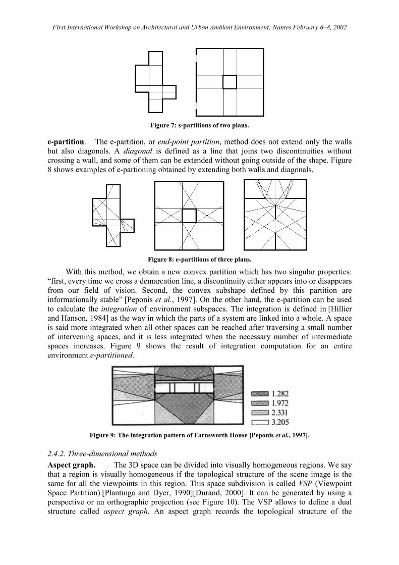
s-partition. The e-partition is an extend of another method proposed by Hillier, calledsurface-partition or s-partition [Hillier, 1996]. The s-partition consists in extending wallsinside the plan, on the same way as the scheme in Figure 7. Hence, we have an environmentdivided by s-lines into s-spaces. Each time an observer crosses an s-line, an entire surfaceeither appears into the visual field or disappears outside it. Thus transitions from one s-spaceto another are associated with changes in the available visual information about shape.However, the reverse is not true. Surfaces and parts of surfaces may appear or disappearwithout crossing an s-line [Peponis et al., 1997].


Figure 7: s-partitions of two plans.

e-partition. The e-partition, or end-point partition, method does not extend only the wallsbut also diagonals. A diagonal is defined as a line that joins two discontinuities withoutcrossing a wall, and some of them can be extended without going outside of the shape. Figure8 shows examples of e-partioning obtained by extending both walls and diagonals.

Figure 8: e-partitions of three plans.

With this method, we obtain a new convex partition which has two singular properties:“first, every time we cross a demarcation line, a discontinuity either appears into or disappearsfrom our field of vision. Second, the convex subshape defined by this partition areinformationally stable” [Peponis et al., 1997]. On the other hand, the e-partition can be usedto calculate the integration of environment subspaces. The integration is defined in [Hillierand Hanson, 1984] as the way in which the parts of a system are linked into a whole. A spaceis said more integrated when all other spaces can be reached after traversing a small numberof intervening spaces, and it is less integrated when the necessary number of intermediatespaces increases. Figure 9 shows the result of integration computation for an entireenvironment e-partitioned.

Figure 9: The integration pattern of Farnsworth House [Peponis et al., 1997].

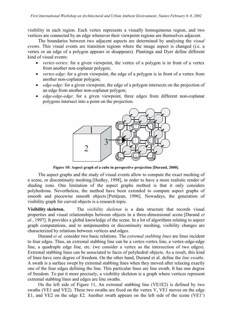
2.4.2. Three-dimensional methodsAspect graph. The 3D space can be divided into visually homogeneous regions. We saythat a region is visually homogeneous if the topological structure of the scene image is thesame for all the viewpoints in this region. This space subdivision is called VSP (ViewpointSpace Partition) [Plantinga and Dyer, 1990][Durand, 2000]. It can be generated by using aperspective or an orthographic projection (see Figure 10). The VSP allows to define a dualstructure called aspect graph. An aspect graph records the topological structure of the


visibility in each region. Each vertex represents a visually homogeneous region, and twovertices are connected by an edge whenever their viewpoint regions are themselves adjacent.

The boundaries between two adjacent aspects are determined by analysing the visualevents. This visual events are transition regions where the image aspect is changed (i.e. avertex or an edge of a polygon appears or disappears). Plantinga and Dyer define differentkind of visual events:

� vertex-vertex: for a given viewpoint, the vertex of a polygon is in front of a vertexfrom another non-coplanar polygon;

� vertex-edge: for a given viewpoint, the edge of a polygon is in front of a vertex fromanother non-coplanar polygon;

� edge-edge: for a given viewpoint, the edge of a polygon intersects on the projection ofan edge from another non-coplanar polygon;

� edge-edge-edge: for a given viewpoint, three edges from different non-coplanarpolygons intersect into a point on the projection.

Figure 10: Aspect graph of a cube in perspective projection [Durand, 2000].

The aspect graphs and the study of visual events allow to compute the exact meshing ofa scene, or discontinuity meshing [Hedley, 1998], in order to have a more realistic render ofshading zone. One limitation of the aspect graphs method is that it only considerspolyhedrons. Nevertheless, the method have been extended to compute aspect graphs ofsmooth and piecewise smooth objects [Petitjean, 1996]. Nowadays, the generation ofvisibility graph for curved objects is a research topic.

Visibility skeleton. The visibility skeleton is a data structure that records visualproperties and visual relationships between objects in a three-dimensional scene [Durand etal., 1997]. It provides a global knowledge of the scene. In a lot of algorithms relating to aspectgraph computations, and to antipenumbra or discontinuity meshing, visibility changes arecharacterized by relations between vertices and edges.

Durand et al. consider two basic relations. The extremal stabbing lines are lines incidentto four edges. Thus, an extremal stabbing line can be a vertex-vertex line, a vertex-edge-edgeline, a quadruple edge line, etc. (we consider a vertex as the intersection of two edges).Extremal stabbing lines can be associated to faces of polyhedral objects. As a result, this kindof lines have zero degree of freedom. On the other hand, Durand et al. define the line swaths.A swath is a surface swept by extremal stabbing lines when they moved after relaxing exactlyone of the four edges defining the line. This particular lines are line swath. It has one degreeof freedom. To put it more precisely, a visibility skeleton is a graph where vertices representextremal stabbing lines and edges are line swaths.

On the left side of Figure 11, An extremal stabbing line (VE1E2) is defined by twoswaths (VE1 and VE2). These two swaths are fixed on the vertex V, VE1 moves on the edgeE1, and VE2 on the edge E2. Another swath appears on the left side of the scene (VE1’)


which divides the polygon which contains E2. The right side of Figure 11 represents thevisibility skeleton of the scene: each extremal stabbing line is a vertex and each adjacentswath is an adjacent edge.

Figure 11: Visibility skeleton construction.

2.4.3. About space partitioningThere are some drawbacks to partition space into homogeneous regions. For e-partitionmethod, Teller notices that the data amount, the computation time, and the pertinence dependtightly on the definition level required for the model [Teller, 2001]. Hence, discontinuityapparition, frequent in urban scenes, contributes to complicate the e-partition representation.What is more, the method is not appropriated for environments which contain curves.

On the other hand, the aspect graph is not really used in computer graphics because of“the difficulty of robust implementation of exact methods, huge size of data-structure and thelack of obvious and efficient indexing scheme” [Durand, 2000]3.

Some of these remarks are also valid for the visibility skeletons. So, we could ask aboutthe quality of these methods in a view to represent visual events inside a large model of a city,for instance. However, they allow, more locally, to do good study of some environments orobjects.

2.5. ConclusionThere are questions about the realism of a representation. Some methods consider what wereally see and others what we expect to see. But the pertinence of a representation involvesproblems of time and of space in order to generate it. Nevertheless, the methods we surveyprovide a set of techniques which can be highlighted, like spherical projection or spacepartitioning. From another viewpoint, some of them provide good methods for local study ofthe visual perception with a good definition level. However, all of these methods are notsufficient to achieve analysis.

3. Space characterizationA representation is a passive way to provide a new interpretation for a set of objects. Anactive way is to provide also a set of measures to characterize this set, allowing to deduce thesensations produced.

The purpose of this section is to survey some methods which allow to deduce thesensations produce by a space and more specifically by an urban environment.

3.1. IsovistTo analyse the visible space, Benedikt introduced in 1979 the isovists. First used forlandscape analysis, Tandy introduced isovist term in [Tandy, 1967], and presented it as a 3 A good discussion of the pros and the cons is given in [Faugeras et al., 1992].


method of “taking away from the [architectural or landscape] site a permanent record of whatwould otherwise be dependent on either memory or upon an unwieldy number of annotedphotographs.” By using this approach and including the Gibson’s perception theory [Gibson,1966, 1979], Benedikt proposed a set of analytic measures on isovist properties to be appliedto achieve quantitative descriptions of spatial environments. Then, he provides anotherdefinition of isovist:

“An isovist is the set of all points visible from a given vantage point in space and withrespect to an environment.” [Benedikt, 1979]

To have a more formal notation, let P be an environment with a configuration of walls4

and x a vantage point in P . An isovist PxV , (or xV if P is understood) generate from x isthe set of all points in P such as:

� �xyPxyPyV Px �� ,

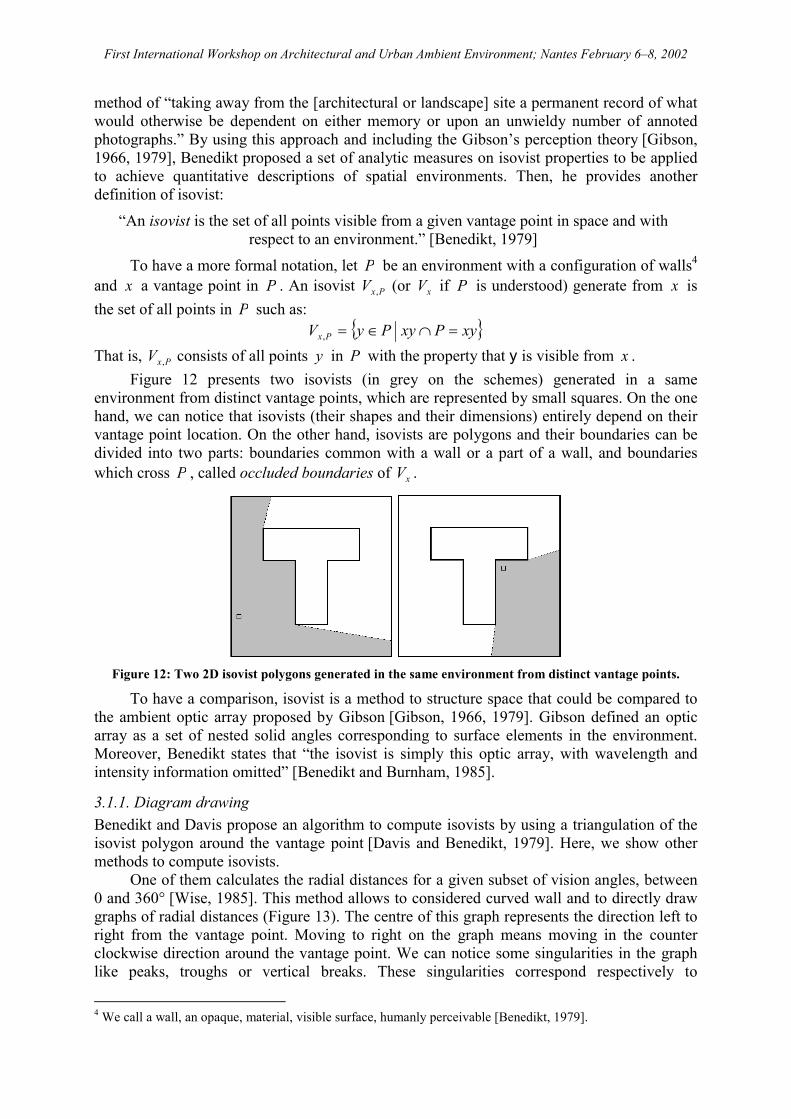
That is, PxV , consists of all points y in P with the property that y is visible from x .Figure 12 presents two isovists (in grey on the schemes) generated in a same

environment from distinct vantage points, which are represented by small squares. On the onehand, we can notice that isovists (their shapes and their dimensions) entirely depend on theirvantage point location. On the other hand, isovists are polygons and their boundaries can bedivided into two parts: boundaries common with a wall or a part of a wall, and boundarieswhich cross P , called occluded boundaries of xV .

Figure 12: Two 2D isovist polygons generated in the same environment from distinct vantage points.

To have a comparison, isovist is a method to structure space that could be compared tothe ambient optic array proposed by Gibson [Gibson, 1966, 1979]. Gibson defined an opticarray as a set of nested solid angles corresponding to surface elements in the environment.Moreover, Benedikt states that “the isovist is simply this optic array, with wavelength andintensity information omitted” [Benedikt and Burnham, 1985].

3.1.1. Diagram drawingBenedikt and Davis propose an algorithm to compute isovists by using a triangulation of theisovist polygon around the vantage point [Davis and Benedikt, 1979]. Here, we show othermethods to compute isovists.

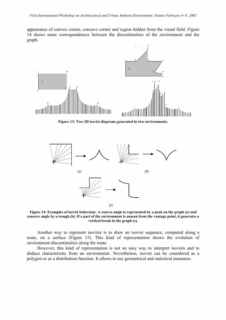
One of them calculates the radial distances for a given subset of vision angles, between0 and 360° [Wise, 1985]. This method allows to considered curved wall and to directly drawgraphs of radial distances (Figure 13). The centre of this graph represents the direction left toright from the vantage point. Moving to right on the graph means moving in the counterclockwise direction around the vantage point. We can notice some singularities in the graphlike peaks, troughs or vertical breaks. These singularities correspond respectively to

4 We call a wall, an opaque, material, visible surface, humanly perceivable [Benedikt, 1979].


appearance of convex corner, concave corner and region hidden from the visual field. Figure14 shows some correspondences between the discontinuities of the environment and thegraph.

Figure 13: Two 2D isovist diagrams generated in two environments.

Figure 14: Examples of isovist behaviour. A convex angle is represented by a peak on the graph (a) andconcave angle by a trough (b). If a part of the environment is unseen from the vantage point, it generates a

vertical break in the graph (c).

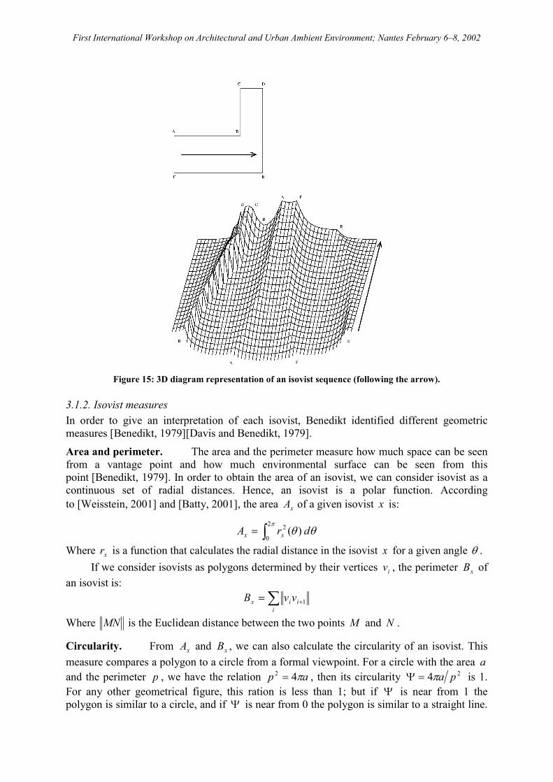
Another way to represent isovists is to draw an isovist sequence, computed along aroute, on a surface (Figure 15). This kind of representation shows the evolution ofenvironment discontinuities along the route.

However, this kind of representation is not an easy way to interpret isovists and todeduce characteristic from an environment. Nevertheless, isovist can be considered as apolygon or as a distribution function. It allows to use geometrical and statistical measures.


Figure 15: 3D diagram representation of an isovist sequence (following the arrow).

3.1.2. Isovist measuresIn order to give an interpretation of each isovist, Benedikt identified different geometricmeasures [Benedikt, 1979][Davis and Benedikt, 1979].

Area and perimeter. The area and the perimeter measure how much space can be seenfrom a vantage point and how much environmental surface can be seen from thispoint [Benedikt, 1979]. In order to obtain the area of an isovist, we can consider isovist as acontinuous set of radial distances. Hence, an isovist is a polar function. Accordingto [Weisstein, 2001] and [Batty, 2001], the area xA of a given isovist x is:

��

�

��2

0

2 )( drA xx

Where xr is a function that calculates the radial distance in the isovist x for a given angle � .If we consider isovists as polygons determined by their vertices iv , the perimeter xB of

an isovist is:� �

�

iiix vvB 1

Where MN is the Euclidean distance between the two points M and N .

Circularity. From xA and xB , we can also calculate the circularity of an isovist. Thismeasure compares a polygon to a circle from a formal viewpoint. For a circle with the area aand the perimeter p , we have the relation ap �42

� , then its circularity 24 pa�� is 1.For any other geometrical figure, this ration is less than 1; but if � is near from 1 thepolygon is similar to a circle, and if � is near from 0 the polygon is similar to a straight line.


The circularity x� for an isovist x is thus the ratio:

2

4

x

xx B

A��

In his papers, Benedikt uses two other forms to calculate the circularity [Benedikt,1979][Davis and Benedikt, 1979]. The first one is given by an inversion

� �xxxx ABN �41 2�� ; the second one is called compactness and is given by xx AB 2 . For

Batty [Batty, 2001], the compactness can be calculated by the ratio between the mean radiallength and the maximal radial length for an isovist, or by the ratio � � � � xxx BA �� 2 .Finally, Conroy [Conroy, 2001] provides another circularity equation where the perimeter isreplaced by mean radial distance of the isovist: � � xxx Ar 2

�� . The circularity formula usedhere is equivalent to the circularity formula used by Teller for open spacescomputation [Teller, 2001] (see section 3.3).

Variance and skewness. Benedikt proposes two other measures. The first one is calledthe variance and calculates the dispersion of the perimeter relative to the vantage point x . Thesecond one is the skewness and calculates the asymmetry of the dispersion of the perimeter tox .

In order to calculate these two measures, Benedikt uses the second and the third radialmoment xM ,2 and xM ,3 . The p-th centred radial moment xpM , for an isovist x is given by:

� ��

drrM pxxxp )).((

21

,

Where �� drr xx ).( is the mean value of function xr . The second radial moment allows

to calculate the standard deviation coefficient which is given by xx M ,2�� and could becompared to the equivalent method of Teller (see section 3.3).

Drift. Another measure is provided by Conroy, called drift, which calculates distancebetween the location from which the isovist is generated and its centre of gravity [Conroy,2001]. Drift tends to be minimal at the centre of spaces and along centre-line of roads.

3.1.3. Applications of isovistsIsovists can be helpful to solve some problems where the visibility is a predominating factor.One of them consists to preserve the privacy. The problem is to find “[...] an optimum balance[...] between the ‘information’ which comes to a person and that which he puts out” [Canterand Kenny, 1975]. Isovist size measures, such as xA and xB , approximate the amount of thiskind of information [Benedikt, 1979]. Other problems consist in seeing much without beingoverly exposed or reduce the security by minimizing the occlusivity fields (spaces leavedunseen from a point), for example. This kind of problems can be treated using isovist theory.

In his report [Wise, 1985], Wise used isovist in order to improve the design of spatialcabins. For him, there are three main concepts: the visual aspects, the kinaesthetic aspects andthe social logic (with the same meaning as [Hillier and Hanson, 1984]). For the visual aspect,Wise was interested in the perceived size of an environment, its apparent orientation and itsaffective connotation. The isovist analysis allowed him to have a direct method to measurevisual qualities.

Finally, an isovist variation, called viewshed, is used in landscape analysis [Burrough,1986][Fisher, 1995]. The originality of this method is that it takes into account the levelinformations of all portion of the ground. Hence, the viewscheds allow to locate the hiddendips from a viewpoint and also the ground area visible from this point.


3.2. Visibility graphs from Space SyntaxInstead of representing the visibility area as isovist do, Turner et al. provides a data structure,called visibility graph, representing the intervisibility relationships between points of anenvironment [Tuner and Penn, 1999][Turner et al., 2001][Turner, 2001].

The visibility graphs are topological graphs where each vertex is associated to a vantagepoint on a map. The presence of an edge between two vertices involves that one “can see” and“can be seen from” the other. Each vertex is disposed regularly on a virtual grid. Inmathematical terms, let � �EVG ,� be a visibility graph, where � �nvvvV ,,, 21 �� is a set ofvertices and � �njieE ij ,,1, �� a set of edges. Each vertex vi is associated to a location� �yx, on a map, and we denote the edge joining iv and jv as ije . In a visibility graph, there isan edge ije if and only if iv can see jv and jv can see iv (this involves Eee jiij �, ).

Figure 16 shows the beginning of a visibility graph construction. We can notice that thewhite vertex neighbourhood is included in the isovist generated by these vertices (in grey onthe scheme). When the visibility graph construction is completed, this property allows us tomeasure visibility informations on each vertex without generating corresponding isovist.

Figure 16: A step in the visibility graph construction.

3.2.1. Visibility graph measuresLike isovist analysis, the visibility graphs were mainly applied to house planning. However,in [Batty, 2001], Batty extended visibility graph applications to urban analysis.

In this paper, we will introduce the possible measures in urban scene by illustratingthem with an actual case in Nantes. We present an analysis, with our implementation ofvisibility graph, of place du Martray and a part of rue Sarrazin in Nantes. This two urbanlocations are relatively enclosed locations and easy to model5. With a 12 906 vertices divisionon a 205 m�265 m map, each vertex covers a surface of 1.4 m2. The Figure 17 shows themodel and the studied part. Considering an outlying zone, enables to have more realisticmeasures for the studied zone.

5 There is another reason why we choose these locations that we will explain later.


Figure 17: The study area corresponds approximately to the grey zone. It corresponds to the place duMartray (a) and a part of the rue Sarrazin (b) in Nantes.

Neighbourhood size. One of the first measure proposed by Turner et al. is theneighbourhood size iN which calculates the adjacent vertices number for each vertex. Aseach vertex covers small map surface, the neighbourhood size of vertex vi is proportional tothe isovist area Ai for the vantage point it represents.

� � .. EevNA ijjii ��

Where � is a coefficient corresponding to the part of surface covered by each vertex. On theupper left of Figure 18, we represent the neighbourhood size for each vertex on the map. Thedarker is a point, the larger is its visibility area.

Clustering coefficient. Another measure, provided by Turner et al., is the clusteringcoefficient i� . It compares the number of adjacent edges in the neighbourhood of a vertexwith its theoretical maximum:

� �� 1 .

,

�

��

�

ii

ikjjki NN

NvvEe�

The clustering coefficient gives a measure of the apparent space convexity from alocation. If i� is near from 1, the most part of the vertices in the neighbourhood are visible

between them. This implies that the generated isovist would be convex. If i� is near from 0,

then the space looks like a star. Another way to interpret i� is about the visibility information

preservation. By moving inside a region where i� is near from 1, the changes of information

would be less important than moving inside a region where the i� is near from 0.

Mean shortest path length. The shortest path between two vertices iv and jv in a graph

is the least number of edges ijd between them. The mean shortest path length iL for a vertex

iv is simply the average of the shortest path lengths from that vertex to every other vertices inthe graph.


V

dL Vv

ij

ij

��

�

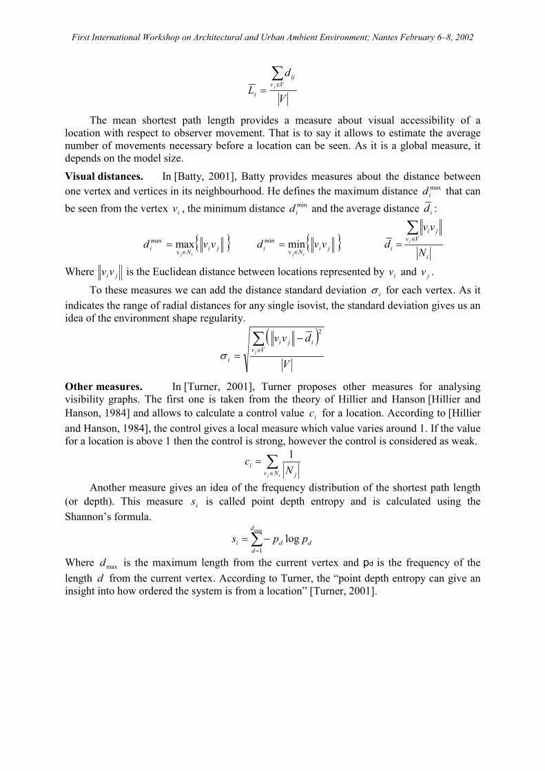
The mean shortest path length provides a measure about visual accessibility of alocation with respect to observer movement. That is to say it allows to estimate the averagenumber of movements necessary before a location can be seen. As it is a global measure, itdepends on the model size.

Visual distances. In [Batty, 2001], Batty provides measures about the distance betweenone vertex and vertices in its neighbourhood. He defines the maximum distance max

id that canbe seen from the vertex iv , the minimum distance min

id and the average distance id :

� � maxjv

maxjiNi vvd

i�

� � � minjv

minjiNi vvd

i�

�

i

Vvji

i N

vvd j

��

�

Where jivv is the Euclidean distance between locations represented by iv and jv .

To these measures we can add the distance standard deviation i� for each vertex. As itindicates the range of radial distances for any single isovist, the standard deviation gives us anidea of the environment shape regularity.

� �

V

dvvVv

iji

ij

��

�

�

2

�

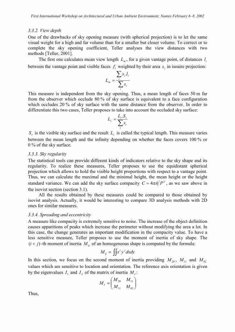
Other measures. In [Turner, 2001], Turner proposes other measures for analysingvisibility graphs. The first one is taken from the theory of Hillier and Hanson [Hillier andHanson, 1984] and allows to calculate a control value ic for a location. According to [Hillierand Hanson, 1984], the control gives a local measure which value varies around 1. If the valuefor a location is above 1 then the control is strong, however the control is considered as weak.

��

�

ij Nv ji N

c 1

Another measure gives an idea of the frequency distribution of the shortest path length(or depth). This measure is is called point depth entropy and is calculated using theShannon’s formula.

��

��

max

1

logd

dddi pps

Where maxd is the maximum length from the current vertex and pd is the frequency of thelength d from the current vertex. According to Turner, the “point depth entropy can give aninsight into how ordered the system is from a location” [Turner, 2001].


Figure 18: Six measures on a 12 906 vertices graph (from upper left to lower right): visibility area,clustering coefficient, integration ratio, maximum distance, average distance, distance standard deviation.

3.2.2. Comments on resultsAt first sight, it is not easy to distinguish the six pictures in Figure 18. For Place du Martray,a division appears with the clustering coefficient, the maximum distance, and the distancestandard deviation due to dead end in the north of Rue Sarrazin. With the other measures, thebrightness from all locations of the place is relatively the same and seems to delimit it. ForRue Sarrazin, the measures have interesting value in the east end, and near Place du Martray.Inside the street, they do not seem to vary a lot. Near Place du Martray and in the east side ofthe street, the space shape is not convex and provides more visibility area; this implies a localdarkening of the coefficients.

Actually, the cathedral appears in the visual field when we walk in the east side of rueSarrazin. It is cathédrale Saint-Pierre located 700 m far from the studied area. It is not shownin figure 16 and would not be correctly studied by the visibility graph even if it were drawnon the map. This is done because of walls which stand between the viewpoint and thecathedral. But as they are in a dip, they are taken into account by two-dimensional methods6,though they do not appear in the visual field. This particularity shows a mistake linked to themap transformation of the urban environment.

3.2.3. Visibility graph criticismWith visibility graph, Turner et al. provide a regular data structure that helps to analyse 6 The same problem appears with the isovist method.


visibility in 2D environments [Turner and Penn, 1999][Turner et al., 2001][Turner, 2001]7. Itsmain advantage is to structure environment and to record visibility informations which isconsidered as a first-order relation. In fact, visibility graph analysis can be considered as anextend or an alternative to isovist field analysis (see section 3.1).

However, we can highlight two weaknesses for the visibility graph method. Above, wehave seen the results of this method could be altered by the two-dimensional transformationof the urban environment. In an other viewpoint, the computation time of the visibility graphincreases rapidly with its resolution. For example, let’s suppose an empty square environmentwhich is 5 km length for each edge. For a definition of 1 m2 per vantage point, it is necessaryto generate one million points, producing a matrix of 6.25�1014 elements for the graphrepresentation. As some algorithms are )( 2nO in the worst case (like the algorithm for graphconstruction or the measure for the mean shortest path length)8, the processing time wouldtheoretically be around one billion (1012) years with an 1 GHz computer. But, a solution tosolve this problem would perhaps be to optimise these algorithms.

Thus, the visibility graph method seems to be adapted to analyse parts of a plane city, orlarger models with a lower but sufficient resolution.

3.3. Open space indicatorsUnlike isovist or visibility graph analysis methods, Dupagne and Teller consider the thirddimension and analyse the urban scene through the spherical projection. Dupagne and Tellerreuse the “urban boxes” concept from Camillo Sitte, and analyse shapes formed by buildings[Dupagne et al., 1997][Teller and Azar, 2001][Teller, 2001].

3.3.1. Sky openingSky opening is defined as the ratio between the sky area in isoaire projection and the area ofthe circle in which image is projected. This coefficient is relative to the enclosure sensation ina scene: it is valuated to 0 in a closed volume and to 1 on a plane without any object.

In a urban scene, the sky opening coefficient changes with the observer location. Near awall, the scene seems to be more closed than in the middle of a street or of a place. It ispossible then to draw the sky opening coefficient variation on a map. Figure 19 shows the skyopening coefficient variation map for la Grand’Place d’Arras [Teller, 2001]. We can noticethe coefficient values in the streets, near the wall in places and in the middle of places.

Figure 19: Sky opening map for la Grand’Place d’Arras [Teller, 2001].

7 The visibility graph analysis functions are implemented in a software called Depthmap, available athttp://www.vr.ucl.ac.uk/depthmap.8 A )( 2nO algorithm has a computation time proportional to the square number of data.


3.3.2. View depthOne of the drawbacks of sky opening measure (with spherical projection) is to let the samevisual weight for a high and far volume than for a smaller but closer volume. To correct or tocomplete the sky opening coefficient, Teller analyses the view distances with twomethods [Teller, 2001].

The first one calculates mean view length mL , for a given vantage point, of distances ilbetween the vantage point and visible faces if weighted by their area is in isoaire projection:

�

��

ii

iii

m s

lsL

.

This measure is independent from the sky opening. Thus, a mean length of faces 50 m farfrom the observer which occlude 80 % of sky surface is equivalent to a face configurationwhich occludes 20 % of sky surface with the same distance from the observer. In order todifferentiate this two cases, Teller proposes to take into account the occluded sky surface:

��

ii

iic s

SLL

.

rS is the visible sky surface and the result cL is called the typical length. This measure variesbetween the mean length and the infinity depending on whether the faces covers 100 % or0 % of the sky surface.

3.3.3. Sky regularityThe statistical tools can provide different kinds of indicators relative to the sky shape and itsregularity. To realize these measures, Teller proposes to use the equidistant sphericalprojection which allows to hold the visible height proportions with respect to a vantage point.Thus, we can calculate the maximal and the minimal height, the mean height or the heightstandard variance. We can add the sky surface compacity 24 PAC �� , as we saw above inthe isovist section (section 3.1).

All the results obtained by these measures could be compared to those obtained byisovist analysis. Actually, it would be interesting to compare 3D analysis methods with 2Dones for similar measures.

3.3.4. Spreading and eccentricityA measure like compacity is extremely sensitive to noise. The increase of the object definitioncauses apparitions of peaks which increase the perimeter without modifying the area a lot. Inthis case, the change generates an important modification in the compacity value. To have aless sensitive measure, Teller proposes to use the moment of inertia of sky shape. The

)( ji � -th moment of inertia ijM of an homogeneous shape is computed by the formula:

�� dxdyyxM jiij

In this section, we focus on the second moment of inertia providing 20M , 11M and 02Mvalues which are sensitive to location and orientation. The reference axis orientation is givenby the eigenvalues 1I and 2I of the matrix of inertia IM :

��

��

��

0211

1120

MMMM

M I

Thus,


� �

24 11

202200220

1

MMMMMI

��

�

� �

24 11

202200220

2

MMMMMI

��

�

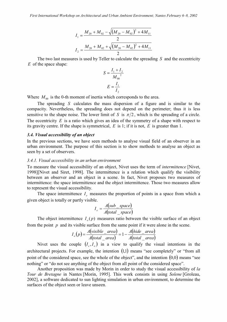
The two last measures is used by Teller to calculate the spreading S and the eccentricityE of the space shape:

200

21

MII

S�

�

2

1

II

E �

Where 00M is the 0-th moment of inertia which corresponds to the area.The spreading S calculates the mass dispersion of a figure and is similar to the

compacity. Nevertheless, the spreading does not depend on the perimeter; thus it is lesssensitive to the shape noise. The lower limit of S is 2� , which is the spreading of a circle.The eccentricity E is a ratio which gives an idea of the symmetry of a shape with respect toits gravity centre. If the shape is symmetrical, E is 1; if it is not, E is greater than 1.

3.4. Visual accessibility of an objectIn the previous sections, we have seen methods to analyse visual field of an observer in anurban environment. The purpose of this section is to show methods to analyse an object asseen by a set of observers.

3.4.1. Visual accessibility in an urban environmentTo measure the visual accessibility of an object, Nivet uses the term of intermittence [Nivet,1998][Nivet and Siret, 1998]. The intermittence is a relation which qualify the visibilitybetween an observer and an object in a scene. In fact, Nivet proposes two measures ofintermittence: the space intermittence and the object intermittence. Those two measures allowto represent the visual accessibility.

The space intermittence eI measures the proportion of points in a space from which agiven object is totally or partly visible.

� �� spacetotalA

spacesubAIe __

�

The object intermittence )( pIo measures ratio between the visible surface of an objectfrom the point p and its visible surface from the same point if it were alone in the scene.

� ��

� �� areatotalA

areahideAareatotalAareavisibleApIo _

_1__

��

Nivet uses the couple � �oe II , in a view to qualify the visual intentions in thearchitectural projects. For example, the intention � �1,1 means “see completely” or “from allpoint of the considered space, see the whole of the object”, and the intention � �0,0 means “seenothing” or “do not see anything of the object from all point of the considered space”.

Another proposition was made by Morin in order to study the visual accessibility of laTour de Bretagne in Nantes [Morin, 1995]. This work consists in using Solene [Groleau,2002], a software dedicated to sun lighting simulation in urban environment, to determine thesurfaces of the object seen or leave unseen.


3.4.2. Object visibility and landscape protectionKoglin and Rheinert [Koglin and Rheinert, 1999] propose a method for generating an optimalsolution in order to build overhead lines. Their method is based on cost criterion, on opticalimpact criterion, and on “approval ability” criterion. To solve the optical impact criterion ofoverhead lines, they use a method developed at Saarland University [Koglin and Zewe, 1995]that takes into account the virtual size of the pylon looked at and the colour differencebetween pylon and background.

In their paper [Koglin and Zewe, 1995, 1996], Koglin and Zewe provide differentmeasures mainly based on method of Groß [Groß, 1991]. The psychophysical factors relate tothe observer density or the observer attention. The physical factors are given below.

� The solid angle � is a measure of the apparent size of an object. It is calculated as theratio between the object visible surface and the square of the visual distance from theobserver ( 2dS�� ).

� The colour difference E� between the object and the background. The difference iscalculated as the geometric distance between the colour values using the CIE Yxycolour space (where Y is the luminance, and x and y the colour location in the chart).Moreover, colours in the landscape depend on the atmospheric attenuation.

As a basis, these factors help to draw up a method for calculating the visibility of anobject. One of the first measure is called the location-specific visibility S �� . It calculates theoptical impact of an object at a particular observer location. We suppose that each observeroccupies an area A� of size 1 m2.

��

��

1 dEA

S

The total visibility � ��A

dASS

gives a measure of entire visual impression caused by an

object in the landscape. On the other hand, the efficiency of camouflage calculates thelocation-specific visibility for the same object from the same observer point but in front of aclear sky and without any obstacle leads to the maximum location-specific visibility maxS �� .

max

max

SSS

��

��

3.5. About methods for space characterizationThe methods described here give an original approach to characterize space, and usuallyprovide a set of measures which allow to draw different kinds of visual variation map for agiven environment. However, some of these methods (e.g. isovist, visibility graph, andmethods for landscape analysis) are not adapted to large urban environment. Others methods,like the Nivet’s method, intend to take up any other applications.

4. ConclusionThe visual interpretation of an urban environment needs a way to model it, with the aim tohighlight some visible elements (e.g. shape, colour, visual events, etc.), and to analyse it inorder to provide a characterization of the environment. In this paper, we saw different kinds ofmethods that allow to interpret the visual events.

In the section 2, we have presented several representation methods of visual field and ofvisual events. They provide a set of concepts which can be highlighted. For example, thespherical projection gives a mean to represent the whole visual world; the notations providedby Thiel or Lynch et al. use an abstraction of the visual world to represent what we see; theconvex partition methods structure the environment into visually homogeneous regions.


However, these methods do not allow to achieve analysis. In section 3, we have seen threecomplete methods — isovist, visibility graph and sky opening indicators — that allow toanalyse the visual perception of architectural and urban scene by using tools that come fromstatistics, graph theory, physics, and social logic of space. Other methods attend to onlyconsidered the visual perception of one object in a scene. They qualify the quantity seen ofthis object or the contrast it produces with the background (in order to analyse the efficiencyof the camouflage for this object).

Most of these methods fail to model or analyse entire cities with a high level ofresolution. All of them are reasonably good if the model is reduced to a district or aneighbourhood. Nevertheless, the methods we saw are mainly based on human visual system,in order to have a more intuitive representation of urban environment and to analyse it ashuman do. However, these elements are often limited to shape perception. With the aim toanalyse visual events, it would be interesting to take into account the motion perception. Mostof these methods are able to study it by generating space variation maps. But, they do notintegrate the motion perception. Thus, it is difficult to interpret what a person can observeactually.

Similar questions raise about other attributes analysed by human visual system andabout the visual events during a motion. For example, attributes like colour (study by themethod saw in the section 3.4.2), texture or lighting are directly analysed by human visualsystem but leaved unexploited.

References

D. APPLEYARD, K. LYNCH, and J. R. MYER (1964). The view from the road. MIT Press.

M. BATTY (2001). Exploring isovist fields: space and shape in architectural and urbanmorphology. Environment and Planning B: Planning and Design, 28(1):123–150.

M. L. BENEDIKT (1979). To take hold of space: isovists and isovist fields. Environment andPlanning B, 6:47–65, 1979.

M. L. BENEDIKT and C. A. BURNHAM (1985). Perceiving architectural space: From opticarrays to isovists. Persistance and change, pages 103–114.

P. BOSSELMANN (1998). Representation of Places. University of California Press, 1998.

P. A. BURROUGH (1986). Principles of Geographical Information Systems for Land ResourcesAssessment. Clarendon Press, Oxford.

D. CANTER and C. KENNY (1975). The spatial environment. International University Press,New York.

R. CONROY (2001). Spatial Navigation in Immersive Virtual Environments. PhD thesis,University of London.

G. CULLEN (1961). The Concise Townscape. Butterworth Architecture.

L. S. DAVIS and M. L. BENEDIKT (1979). Computational models of space: Isovists and isovistfields. Computer Graphic and Image Processing, 11(1):49–72.

I. DE WOLFE (1963). The Italian Townscape. Architectural Press, Londres.

A. DUPAGNE, M. JADIN, and J. TELLER (1997). L’espace public de la modernité. Études etDocuments. Ministère de la région wallonne, direction générale de l’aménagement duterritoire, du logement et du patrimoine, division de l’aménagement et de l’urbanisme.F. DURAND (2000). A multidisciplinary survey of visibility. In Proceedings of


SIGGRAPH’2000. [CD-ROM] Course notes CD-ROM, course #04: Visibility: Problems,Techniques, and Applications.

F. DURAND, G. DRETTAKIS, and C. PUECH (1997). The visibility skeleton: A powerful andefficient multi-purpose global visibility tool. In Proceedings of SIGGRAPH’97, pages 89–100, Los Angeles, California.

O. FAUGERAS, J. MUNDY, N. AHUJA, C. DYER, A. PENTLAND, R. JAIN, and K. IKEUCHI(1992). Why aspect graphs are not (yet) practical for computer vision. Computer Vision andImage Understanding: CVIU, 55(2):322–335.

P. F. FISHER (1995). An exploration of probable viewsheds in landscape planning.Environment and Planning B: Planning and Design, 22:527–546.

Georgia Tech Research Corporation (2001). Spatialist. [On-line] URL:http://murmur.arch.gatech.edu/˜spatial.

J. J. GIBSON (1950). The Perception of the Visual World. The Riverside Press, Cambridge,Massachusetts, 1950.

J. J. GIBSON (1966). The Senses Considered as Perceptual Systems. Houghton Mifflin,Boston, MA.

J. J. GIBSON (1979). The Ecological Approach to Visual Perception. Houghton Mifflin,Boston, MA.

D. GROLEAU (2002). Solene : un outil de simulation des éclairements solaires et lumineuxdans les projets architecturaux et urbains. To be published in Actes de l’École Thématique :La modélisation de la ville 2, Nantes, 1999.

M. GROß (1991). The analysis of visibility — environmental interactions between computergraphics, physics, and physiology. Computers & Graphics, 15(3):407–415.

D. HEDLEY (1998). Discontinuity Meshing for Complex Environments. PhD thesis,Department of Computer Science, University of Bristol, August.

B. HILLIER (1996). Space is the Machine. Cambridge University Press.

B. HILLIER and J. HANSON (1984). The social logic of space. Cambridge University Press.

A. HUTCHINSON (1954). Labanotation. New Directions.

H.-J. KOGLIN and RHEINERT (1999). Multiobjective optimization with evolutiionaryalgorithms for the synthesis of optimal overhead lines. In Proceedings of ISAP 1999, Rio deJaneiro.

H.-J. KOGLIN and R. ZEWE (1995). A valuation system for the visibility of overhead lines.Engineering Intelligent Systems, 3(4):195–203.

H.-J. KOGLIN and R. ZEWE (1996). Visibility as a criterion for the approval in the regionalplanning procedure. In Proceedings of 12th Power Systems Computation Conference,Dresden.

K. LYNCH (1960). The image of the city. MIT Press.

M. MORIN (1995). Lecture de la Tour de Bretagne – développement d’un outil de lecture de laville (simulation de l’accessibilité visuelle). TPFE, École d’Architecture de Nantes.

M.-L. NIVET (1998). De Visu : un logiciel pour la prise en compte de l’accessibilité visuelledans le projet architectural, urbain ou paysager. PhD thesis, Université de Nantes.

M.-L. NIVET and D. SIRET (1998). Simulation inverse de l’accessibilité visuelle en mileu


urbain. Revue Internationale de CFAO, 13(1):93–110.

P. PANERAI (1970). Paysage urbain et analyse pittoresque. Archives d’Architecture Moderne,Bruxelles.

P. PANERAI, J.-C. DEPAULE, and M. DEMORGON (1997). Formes urbaines, de l’îlot à la barre.Éditions Parenthèses, Marseille.

P. PANERAI, J.-C. DEPAULE, and M. DEMORGON (1999). Analyse Urbaine. Collectioneupalinos. Éditions Parenthèses.

E. PANOFSKY (1975). La perspective comme forme symbolique. Les éditions de Minuit.

J. PEPONIS, J. WINEMAN, M. RASCHID, S. H. KIM, and S. BAFNA (1997). On the description ofshape and spatial configuration inside buildings: convex patitions and their local properties.Environment and Planning B: Planning and Design, 24(5):761–781.

S. PETITJEAN (1996). The enumerative geometry of projective algebraic surfaces and thecomplexity of aspect graphs. International Journal of Computer Vision, 19(3):1–27, 1996.

H. PLANTINGA and C. R. DYER (1990). Visibility, occlusion, and the aspect graph.International Journal of Computer Vision, 5(2):137–160.

C. R. V. TANDY (1967). The isovist method of landscape survey. Ed. H. C. Murray(Landscape Research Group, London).

J. TELLER (2001). La régulation morphologique dans le cadre du projet urbain : Spécificationd’instruments informatiques destinés à supporter les modes de régulation performantiels.PhD thesis, Université de Liège.

J. TELLER and S. AZAR (2001). Townscope II – A computer system to support solar accessdecisionmaking. Solar Energy Journal, 70(3):187–200.

P. THIEL (1969). La notation de l’espace, du mouvement et de l’orientation. Architectured’Aujourd’hui, 145:49–58.

A. TURNER (2001). Depthmap: A program to perform visibility graph analysis. InProceedings of the 3rd Symposium on Space Syntax, Georgia Institute of Technology.

A. TURNER, M. DOXA, D. O’SULLIVAN, and A. PENN (2001). From isovists to visibilitygraphs: a methodology for the analysis of architectural space. Environment and Planning B:Planning and Design, 28(1):103–121.

A. TURNER and A. PENN (1999). Making isovists syntactic: isovist integration analysis. InProceedings of the 2nd Symposium on Space Syntax, Universisdad de Brasilia, Brazil.

E. W. WEISSTEIN (1999). Concise Encyclopedia of Mathematics CD-ROM. Chapman &Hall/CRCnetBASE. [CD-ROM] edition 1.0.

J. A. WISE (1985). The quantitative modelling of human spatial habitability. Technical ReportNAG 2–346, NASA.

Visual Analysis of Urban Environment

Documents

Transcript of Visual Analysis of Urban Environment