Virtual Tall Towers and Inversionsor

How to Make Productive Useof Continental CO2 Measurements

in Global Inversions

Martha Butler

The Pennsylvania State University

Department of Meteorology

April 24, 2007

TransCom Meeting

mpbutler@met.psu.edu

Outline

• The Problem with Continental CO2 data

• Virtual Tall Tower Overview

• Inversion Setup

• Perfect Data Results

• Continuing Work

Problem Definition

• Continental data are messy: big signal with lots of noise.

• Confounded by boundary layer processes (diurnal, synoptic, seasonal)

• Transport models have problems representing the continental boundary layer, especially near the land surface.

• Most continental observations are made in this surface layer.

• Observation site density does not permit global estimation of fluxes at the resolution we would like, unless we use continental data.

What About Flux Towers?

• CO2 is measured continuously at every continental flux tower, but…

• These data are not required to be either accurate or precise to support CO2 flux calculations.

• What if?

• Flux tower CO2 data could be high precision and calibrated with the global standards (at reasonable cost).

• The data could be “adjusted” (using meteorological and flux data available at the site) to represent a mid-day CO2 mixing ratio value above the surface layer.

• This adjustment adds to the uncertainty of the observation; is it worth it?

What Is This Adjustment?

Following the mixed layer similarity theory of Wyngaard & Brost [1984] and Moeng & Wyngaard [1989], the vertical gradient of a scalar in the boundary layer:

0

* *

izb t

i i i i

wcwcC z zg g

z z w z z w z

where

gb and gt are bottom-up and top-down gradient functions scaled by boundary layer depth zi

w* is the convective velocity scale

wc0 and wczi are the surface and entrainment fluxes of the scalar C

Example Adjusted Time Series

Hourly (mid-day hours) adjusted CO2 mixing ratios for:

Harvard Forest

Northern Old Black Spruce

WLEF

Courtesy of David Tyndall

See also www.amerifluxco2.psu.edu for high-precision, calibrated measurements at flux towers and www.eol.ucar.edu/~stephens/RACCOON/ for the Rocky Mountains sites.

Inversion Setup

• Forward transport model: PCTM, 2.5° longitude x 2° latitude using GEOS-4 met data (3-hr) for 2000, 2001, 2002

• Background fluxes:– Seasonal fossil with 1995 spatial pattern (ORNL)

– SiB3 hourly flux for 2000, 2001, 2002 (CSU)

– Takahashi 2002 ocean

• Matrix inversion in the TransCom3 style solving for monthly fluxes in 36 land regions and 11 ocean regions in 2002

• Forward model sampling strategy: – Entire atmospheric column sampled hourly in 2002 at each observation

location.

– Ten-day means of the atmospheric grid saved for analysis.

Networks Tested (so far)

• 85 station network: NOAA GMD sites active in 2002• 159 station network: NOAA GMD + GAW• 145 station network:

– Remove some profiles and added VTT sites active in 2002

• 165 station network:– Add high-precision, well-calibrated sites active after 2002

• Flux tower/VTT locations• Britt Stephen’s mountain sites• Bev Law’s Oregon transect• 2 established sites in Africa

• 174 station network:– Add a few other sites in under-represented regions

85 Station Network

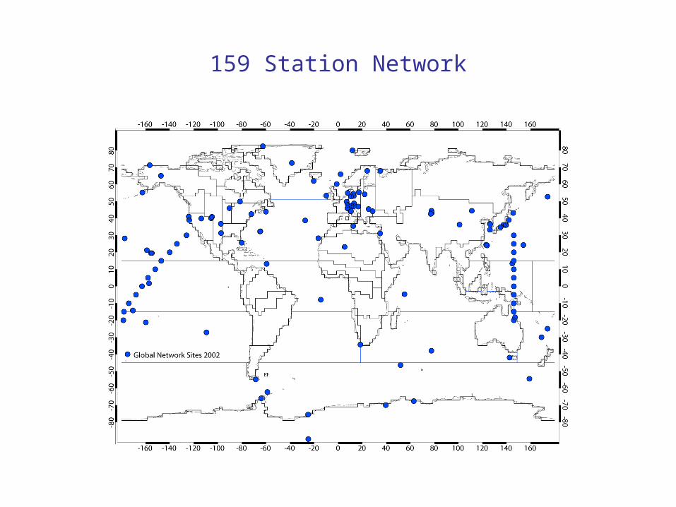
159 Station Network

145 Station Network

165 Station Network

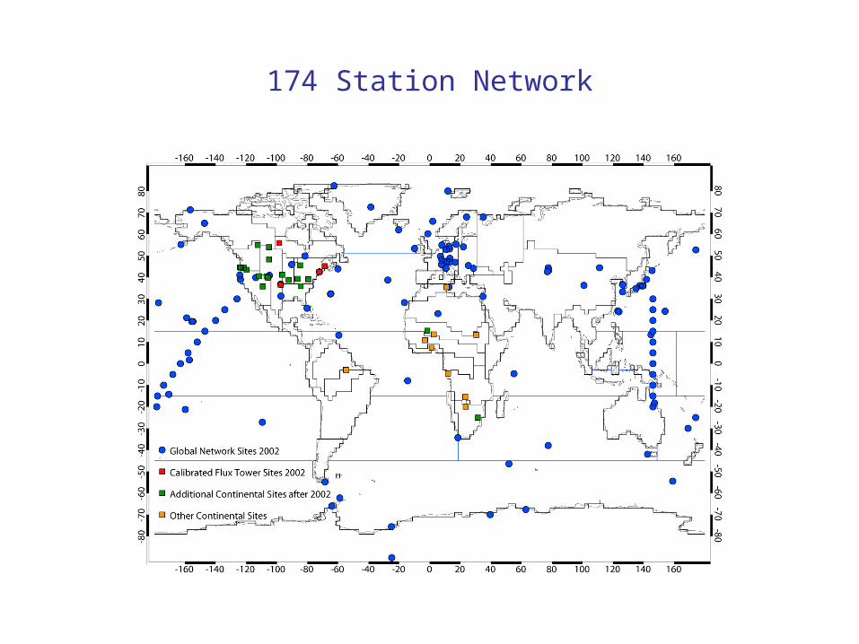
174 Station Network

Tests of the Inversion Setup

• Sensitivity to Choice of Priors & Prior Uncertainty– Priors derived from TransCom3 Seasonal Mean Inversion

– At least 0 ± 2 Gt C/yr for each region

– 0 ± 5 Gt C/yr for each region

– 0 ± 10 Gt C/yr for each region

– At least 0 ± 3 Gt C/yr for each land region, TransCom for ocean regions

• Sensitivity of Posterior Flux Uncertainty to Choice of Networks– Boreal and Temperate North America

– South America

– Africa

Global Aggregated Results

Thick colored lines show posterior flux (and the prior contained in the background flux).

Dashed lines show the posterior uncertainty for the aggregated area for the 85 station network.

Error bars show the posterior uncertainty for the 174 station network.

Note that flux scales differ for land and ocean.

June Posterior Flux Uncertainties

Oregon transect Flux Towers

Flux Towers

Boreal North America and Tropical America

Fraserdale Flux Towers

Tapajos

Examples for the African Regions

Hombori

Skukuza

Continuing Work

• Noisy data tests with simulated observations• Model sampling to match observation times• Preparation of observation data• “The real deal”• Daytime forward pulse runs from land regions

Acknowledgements

• People– Davis Group at Penn State– Denning Group at CSU– Randy Kawa at NASA GSFC

– Everyone, everywhere in the CO2 measurement network

• Funding Agencies– NASA GSRP– NOAA, DOE, NSF– PSU, College of EMS Centennial Travel Grant

Comments and suggestions are welcome!

And thank you!