1

Abstract— In this paper, a machine-to-machine (M2M) networks is arranged hierarchically to support an energy-efficient routing protocol for data transmission from terminal nodes to a sink node via cluster heads in a Wireless Sensor Network (WSN). Network congestion caused by heavy M2M traffic is tackled using load balancing solutions to maintain high levels of network performance. Firstly, a Multilevel Clustering Multiple Sinks (MLCMS) with IPv6 protocol over Low Wireless Personal Area Networks (6LoWPAN) is promoted to prolong network lifetime. Secondly, enhanced network performance is achieved through linear integer-based optimisation.  A Self-Organising Cluster Head to Sink Algorithm (SOCHSA) is proposed, hosting Discrete Particle Swarm Optimisation (DPSO) and Genetic Algorithm (GA) as Evolutionary Algorithms (EAs) to solve the network performance optimisation problem. Network Performance is measured based on Key Performance Indicators (KPIs) for load fairness and average residual network energy. The SOCHSA algorithm is tested by two benchmark problems with two and three sinks. DPSO and GA are compared with the Exhaustive Search (ES) algorithm to analyse their performances for each benchmark problem. Both algorithms achieve optimum network performance evaluation values of 108.059 and 108.1686 in the benchmark problems P1 and P2, respectively.  Using three sinks under the same simulation settings, the average residual energy is improved by 2% when compared to two sinks. Computational results prove that DPSO outperforms GA regarding complexity and convergence, thus being best suited for a proactive Internet of Things (IoT) network. The proposed mechanism satisfies different network performance requirements of M2M traffic by instant identification and dynamic rerouting.

Index Terms— DPSO; GA; IoT; WSN; MLCMS; M2M; 6LoWPAN .

I. INTRODUCTIONhe Internet of Things (IoT) refers to a network of billions of objects that can send and receive data. M2M

communication is considered as the core of IoT, whereby it is seen as is the key to making it a reality, i.e. enhancing the communication of real things in the world, transmitting information and executing smart tasks. Many solutions in the M2M domain have been provided, and it is anticipated that billions of devices will be connected using M2M in the future [1][2]. Machine-to-machine (M2M) networks enabling networked nodes (sensors or actuators) to exchange information have been intensively studied lately, particularly for sensing and surveillance purposes where hundreds or thousands of nodes (devices) densely located over the small or medium area. Some of the key features of M2M include low

T

mobility, Packet switching, time controlled data transmission, monitoring events of interest, low power consumption, and location specific triggering of M2M devices in a particular area.

Moreover, sensors and communication devices are the essential endpoints for any M2M application. However, the endpoints cannot connect directly to the network operator or interconnect, unless supported by WPAN technology standards such as 6LoWPAN, ZigBee, and Bluetooth. Recent technological developments, including M2M, smart grids and smart environment applications, are having a marked impact on the development of Wireless Sensor Networks (WSNs). Moreover, most appliances are equipped with the capabilities for sensing people’s daily needs. However, the efficient use of the limited energy resources of WSN nodes is crucial to these technological advances, regarding which topology control methods are being employed to extend battery lifetime [3], [4]. We envision a future where millions of small sensors, actuators, and other devices can form self-organising wireless networks. This is dependent on the IoT concept, whereby billions of machines will be able to interact and control one another with no human involvement. These devices will connect continuously and bring significant benefits to people in their everyday lives to enhance their wellbeing. Areas that will be significantly improved are: -Healthcare: Wireless systems will able to gather information that will then be passed on to providers of healthcare. The data will then be analysed and subsequently, for instance, decide whether any medical assistance/help is required to a particular individual. -Emergency response: WSNs will gather data about the conditions of different types of infrastructure, including buildings, bridges, and roads. Consequently, the emergency services and other relevant personnel will be informed of any impending failure, such as a bridge collapsing.-Supply chain and inventory management: Materials will be automatically monitored through the supply chain from the raw form to the retail market. Sensors will assess the level of stock and replenish (if required) with little human involvement or perhaps even none further along the line [5][6].

The main aim of topology control in wireless M2M networks is to diminish energy consumption and hence, prolong network lifetime. Because energy efficiency is crucial when designing M2M WSN protocols, the sensor nodes need to function in a self-governing manner with small batteries lasting for several months or even years. Since the replacement of the batteries for a large number of devices is virtually impossible in distant or unfavorable environments, energy is an essential resource in WSNs [7][8]. Hence, keeping power consumption to a minimum is a primary focus for researchers, and the topic has been investigated thoroughly. Energy-efficient transmission protocols for M2M WSN are categorised into routing and clustering types. Clustering in M2M WSN refers to arranging the nodes into

Network Performance Evaluation of M2M With Self Organising Cluster Head to Sink Mapping

Wasan.Twayej, M.Khan, Student Member, IEEE, H.S. Al-Raweshidy, Senior Member, IEEE

2

groups, according to the needs of the network. Every group has a leader called the cluster head (CH), and the rest are just common nodes [9]. This type of protocol substantially reduces energy consumption by aggregating multiple sensed data that are transmitted to the sink node [9]. The clusters can be configured to become more energy-efficient by size and cluster count. However, without this being associated with the position of the sink, this will lead to the network’s topology having clusters with unbalanced residual energy and limited network lifespan.In fact, the sink placement becomes an important criterion for the network designer to increase the network lifetime and system performance. In a WSN, multiple sinks at correct locations can sharply decrease the energy use and the message transfer delay in communication. Moreover, a multiple-sink WSN has much less tendency for sink node isolation [10]. In a large-scale M2M scenario with a single sink WSN, a heavy traffic load may be experienced for packet transmission at the sink, which may lead to heavy packet drops at the sink as well as significant network congestion. Nodes not only gather data within their sensing range, but they also send them to those nodes remote from the sink, which leads to different power consumption among them along with unequal connectivity across the network. Further, during such matters as disaster management, it is preferable that most sensor nodes be near to the sink [11].

Apart from energy consumption efficiency, an important issue is the demand for more IPs as M2M is separated from IoT and needs to communicate a vast number of things. This issue can be addressed by using 6LoWPAN, and its application is rapidly increasing. In particular, it has been playing an important role in enhancing the throughput, which has been somewhat limited, for IEEE 802.15.4. The main reason for designing 6LoWPAN is to pave the way for M2M for supporting a broad range of applications [12].

However, supporting a wide variety of applications can lead to network overload situations. Overload in networks has an adverse impact on performance, which can be addressed through effective load balancing algorithms. These have been widely researched over the last 20 years after the innovations of parallel and distributed computing. The general aim of them is to share the load evenly and fairly amongst all the resources available [13], with the method pursued having a direct impact on network performance [14]. In sum, the key objective of any load balancing algorithm is to improve the computation capability of the system by obtaining fair and balanced use of the available. There are two types of load balancing policies: static and dynamic.

Load balancing in the static dimension assesses the status of the system and application statically in the decision-making process, whereas dynamic policies require system status information to share the workload between the processors at run-time. Information gathered at run-time for each node, determines the processes allocated to the processors. For instance, in an overload situation at a sink, the task causing overload may be reassigned to an underloaded sink. When compared to traffic in a conventional Human-to-Human (H2H)

arrangement, M2M has different issues and characteristics. To begin with, burst traffic generated by an enormous number of devices can lead to a server experiencing heavy processing overhead. Also, quality of service (QoS) can differ, according to the types of traffic from different applications. To deal with heavy network loads while keeping high levels of network performance and enhanced energy efficiency, M2M networks usually employ a load balancing server. However, a major challenge is to achieve fairness of the load in the whole system. The load balancer deals with many simultaneous nodes by re-routing their data to optimum paths thereby allowing the system to scale the service requests further by only adding more nodes in the network. The CPU workload on the sink will increase due to the high processing of data coming from the CHs. Such algorithms, where the nodes are arranged in clusters in the network for data transmission are termed as cluster-based methods [15].

Since sensors are one of the key components of M2M networks that can be deployed in a massive quantity for monitoring or surveillance [4]. The aim of this paper is to improve network performance by integrating an efficient routing protocol (MLCMS) and a load balancing strategy to introduce new transmission techniques while maintaining a more balanced system. A self-organised network (SON) is proposed and is formulated as a linear integer-based constrained optimisation problem, which tries to balance the load among multiple sinks. The load balancing strategy identifies optimum sink for each CH to transmit to, in a multi-sink environment while the MLCMS protocol defines the transmission strategy between nodes, i.e., CH-Sink, Node-CH, and CH-CH as shown in Fig. 1. Note that, self-optimisation is a key feature in SON. However, it itself is an optimisation issue [7].

The MLCMS is also responsible for CH selection satisfying a particular criterion which has a positive impact on network lifetime enhancement. Moreover, the load balancing scheme proposed considers key performance indicators (KPIs) regarding load fairness index and average residual energy to maintain high levels of network performance. The main contributions of this work are highlighted as follows:

1. A new WSN deployment architecture is proposed which supports multiple sinks and layers as shown in Fig. 2, making it suitable for seamless integration in future cloud communication networks for IoT support.

2. A new energy efficient routing protocol (MLCMS) is proposed to support multi-layer CHs selection and transmission to multiple sinks.

3. Since the MLCMS protocol is responsible for CH selection and transmission strategies, the load balancer proposed in the architecture is responsible for identifying optimum CH-Sink configuration by solving an integer-based optimisation problem.

4. The load balancer obtains optimum CH-Sink re-configuration via an algorithm called SOCHSA. Once the load on any sink reaches an alarming threshold, the load balancer triggers SOCHSA algorithm. Two important KPIs are

3

considered to monitor network performance, based on which the optimum CH- Sink setting can be identified. These KPIs are load fairness index and average residual energy.

5. The proposed SOCHSA algorithm hosts two evolutionary algorithms, i.e., GA and DPSO to solve the load balancing optimisation problem. Since the standard GA and PSO cannot be applied directly to the integer-based optimisation problem in this work, a DPSO and real-valued GA are developed to provide the optimum CH-Sink setting. Moreover, both GA and DPSO maximizes an objective function, which is defined as network performance in this paper and is a weighted combination of the two major KPIs dicussed above.

6. To enable every CH with the ability of flexible transmission to any sink based on the CH-Sink configuration, a sharing node with unlimited energy is employed in the architecture as shown in Fig.1 and Fig.3. The sharing nodes make the co-operative operation of MLCMS protocol and SOCHSA possible, without affecting the transmission ranges defined by the MLCMS protocol.

The remainder of the paper is organised as follows. Section II presents the related work while Section III discusses the standards. The system model architecture and the energy model employed are presented in Section IV. The proposed load balancing scheme and its computational results when compared different algorithms are covered in Section V and Section VI, respectively. Finally, the concluding remarks are provided in Section VII.

II.RELATED WORK

To enhance the performance of WSN clustering techniques have been widely researched ([8]; [9]; [10]). Prior work is reviewed based on a metaheuristic perspective. The energy balanced unequal clustering protocol (EBUC) [11] is a centralised clustering protocol, with which the creators aimed to surmount the hot-spot problem through the creation of unequal clusters by deploying centralised PSO algorithm at the base station (BS). The clusters are created so that those close to the BS have fewer nodes, which thus increases cluster numbers in its proximity. Regarding cluster-cluster communication, a greedy algorithm is deployed to choose a relay node according to its distance from the BS and residual energy. A centralised clustering protocol, which involves energy-aware clustering for WSNs implementing a PSO algorithm (PSO-C) at the BS, was put forward in [12]. The available node energy and the distances between the CHs are considered in this protocol. An objective function that is aimed at minimising the maximum average Euclidean distance of the nodes to their linked CHs, as well as the ratio of the aggregated starting energy of the nodes to the total energy of those CHs that are candidates, is defined. Also, the protocol warrants those nodes with enough energy can be chosen to be CHs. LEACH and LEACH-C about the network lifetime and the throughput are both outperformed by PSO-C. Moreover, [12] has demonstrated that regarding convergence time, network lifetime and data delivery, this algorithm also surpasses GA and K-means-based clustering protocols

regarding performance. An earlier protocol based on GA aimed at selecting CHs so as to minimise the total network distance can be found in [13]. The objective function is the minimisation of the aggregate distance between the cluster members and their allocated CHs along with the distance of the latter to the BS. As with PSO-C, it too warrants nodes having sufficient energy can be chosen as CHs. An energy-ware evolutionary routing protocol (EAERP) was proposed by [14]. This involves a centralised single-hop clustering protocol with the BS running an evolutionary-based protocol for optimising CH election and the subsequent forming of clusters. Minimising the total dissipated energy across the network is defined as the objective function. This is calibrated as the total energy expended by the non-CHs in dispatching data signals to their CHs as well as the aggregate energy utilised by the latter to total the data signals and to send these signals to the BS. The energy consumption model as defined by [15] is deployed to calculate the energy expended in the process of the transmission and reception of data. [16] has advanced a GA-based protocol to address the problem of load balance amongst CHs. This creates clusters such that the maximum load for all the CHs is minimised. The CHs are identified a priori, with the objective to optimise the ratio of non-CH nodes to CHs to get cluster balancing. Minimising the standard deviation of the CH load is the objective function, which provides an even sharing of the load for each cluster.

Regarding network performance, [17] improves the WSN performance by tackling the issues of collision and interference, which are inherited from increased number of nodes in the network. This is because with increased number of nodes in the network, packet collision and communication interference are maximized. The authors in [17] proposed a node concentration-driven gossiping (CG-AODV) algorithm to address the collision and interference challenges in Ad-hoc On-demand Distance Vector (AODV) routing protocol.

The key difference between the proposed work and previous works are in the application of EAs for re-configuration of CHs to sinks and considering optimum residual energy in whole network sensor nodes. In contrast to previous studies on clustering and optimisation in WSNs, the proposed work consider important factors like enhanced clustering and transmission techniques along with load balancing among multiple sinks (rather than in only in CHs), especially when considering M2M technologies and IoT networks.

III. IETF STANDARDS

In 2003, the IEEE and Internet Engineering Task Force (IETF) standardisation bodies began constructing a framework for the communication protocols of IoT systems [18]. Recently, the 6LoWPAN working group (WG) invented an adaptation layer, which delivers compression of the header of IPv6 and fragmentation for the datagram. Also, for low power packet transmission over 802.15.4, the WG has focused on providing better IPv6 connectivity, rather than constrained node networks [19]. Most hierarchical networks use a routing

4

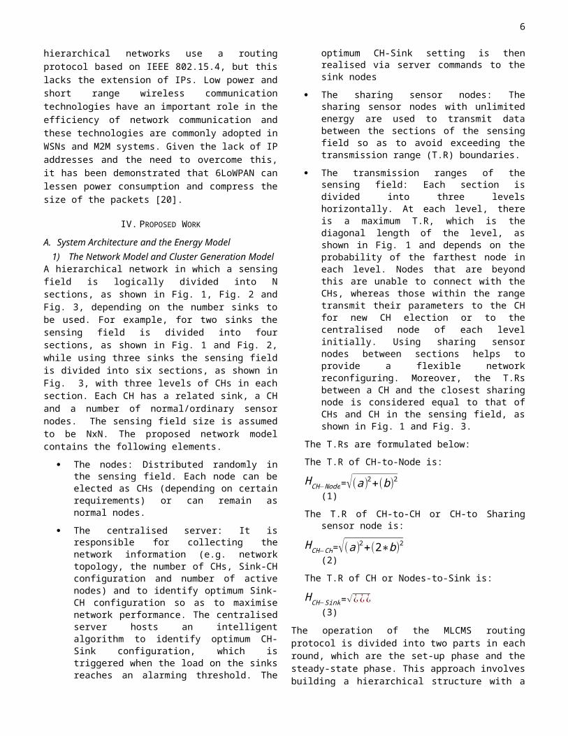
protocol based on IEEE 802.15.4, but this lacks the extension of IPs. Low power and short range wireless communication technologies have an important role in the efficiency of network communication and these technologies are commonly adopted in WSNs and M2M systems. Given the lack of IP addresses and the need to overcome this, it has been demonstrated that 6LoWPAN can lessen power consumption and compress the size of the packets [20].

IV. PROPOSED WORK

A. System Architecture and the Energy Model1) The Network Model and Cluster Generation Model

A hierarchical network in which a sensing field is logically divided into N sections, as shown in Fig. 1, Fig. 2 and Fig. 3, depending on the number sinks to be used. For example, for two sinks the sensing field is divided into four sections, as shown in Fig. 1 and Fig. 2, while using three sinks the sensing field is divided into six sections, as shown in Fig. 3, with three levels of CHs in each section. Each CH has a related sink, a CH and a number of normal/ordinary sensor nodes. The sensing field size is assumed to be NxN. The proposed network model contains the following elements.

The nodes: Distributed randomly in the sensing field. Each node can be elected as CHs (depending on certain requirements) or can remain as normal nodes.

The centralised server: It is responsible for collecting the network information (e.g. network topology, the number of CHs, Sink-CH configuration and number of active nodes) and to identify optimum Sink-CH configuration so as to maximise network performance. The centralised server hosts an intelligent algorithm to identify optimum CH-Sink configuration, which is triggered when the load on the sinks reaches an alarming threshold. The optimum CH-Sink setting is then realised via server commands to the sink nodes

The sharing sensor nodes: The sharing sensor nodes with unlimited energy are used to transmit data between the sections of the sensing field so as to avoid exceeding the transmission range (T.R) boundaries.

The transmission ranges of the sensing field: Each section is divided into three levels horizontally. At each level, there is a maximum T.R, which is the diagonal length of the level, as shown in Fig. 1 and depends on the probability of the farthest node in each level. Nodes that are beyond this are unable to connect with the CHs, whereas those within the range transmit their parameters to the CH for new CH election or to the centralised node of each level initially. Using sharing sensor nodes between sections helps to provide a flexible network reconfiguring. Moreover, the T.Rs between a CH and the closest sharing node is considered equal to that of CHs and CH in the sensing field, as shown in Fig. 1 and Fig. 3.

The T.Rs are formulated below:

The T.R of CH-to-Node is:

HCH−Node=√(a)2+(b)2 (1)

The T.R of CH-to-CH or CH-to Sharing sensor node is:

HCH−CH=√(a)2+(2∗b)2 (2)

The T.R of CH or Nodes-to-Sink is:

HCH− Sink=√¿¿¿ (3)

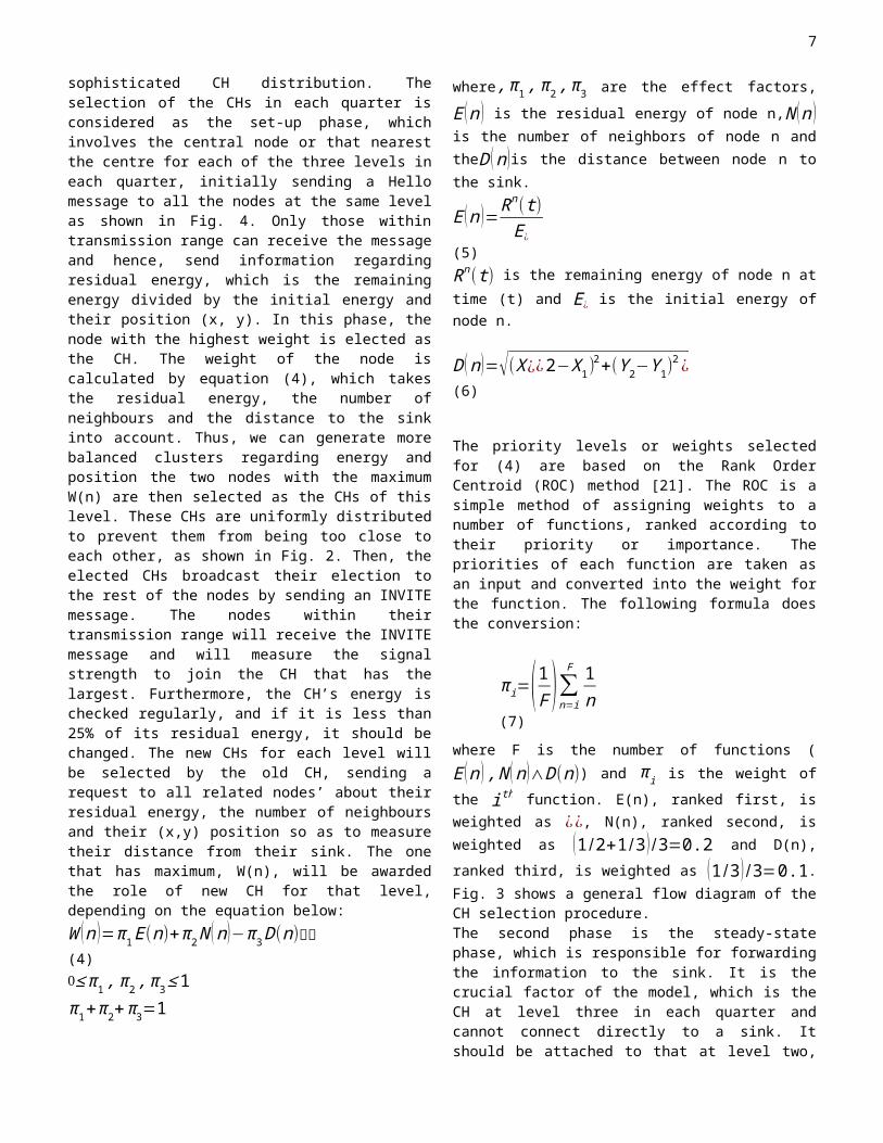
The operation of the MLCMS routing protocol is divided into two parts in each round, which are the set-up phase and the steady-state phase. This approach involves building a hierarchical structure with a sophisticated CH distribution. The selection of the CHs in each quarter is considered as the set-up phase, which involves the central node or that nearest the centre for each of the three levels in each quarter, initially sending a Hello message to all the nodes at the same level as shown in Fig. 4. Only those within transmission range can receive the message and hence, send information regarding residual energy, which is the remaining energy divided by the initial energy and their position (x, y). In this phase, the node with the highest weight is elected as the CH. The weight of the node is calculated by equation (4), which takes the residual energy, the number of neighbours and the distance to the sink into account. Thus, we can generate more balanced clusters regarding energy and position the two nodes with the maximum W(n) are then selected as the CHs of this level. These CHs are uniformly distributed to prevent them from being too close to each other, as shown in Fig. 2. Then, the elected CHs broadcast their election to the rest of the nodes by sending an INVITE message. The nodes within their transmission range will receive the INVITE message and will measure the signal strength to join the CH that has the largest. Furthermore, the CH’s energy is checked regularly, and if it is less than 25% of its residual energy, it should be changed. The new CHs for each level will be selected by the old CH, sending a request to all related nodes’ about their residual energy, the number of neighbours and their (x,y) position so as to measure their distance from their sink. The one that has maximum, W(n), will be awarded the role of new CH for that level, depending on the equation below: W (n )=ϖ1 E (n)+ϖ2 N ( n )−ϖ 3 D(n) (4)≤ ϖ1 , ϖ2 , ϖ3 ≤ 1ϖ1+ϖ2+ϖ3=1

5

where, ϖ1 , ϖ2 , ϖ3 are the effect factors, E (n ) is the residual energy of node n,N (n ) is the number of neighbors of node n and theD (n )is the distance between node n to the sink.

E (n )=Rn( t)E¿

(5)Rn(t ) is the remaining energy of node n at time (t) and E¿ is the initial energy of node n.

D (n )=√(X ¿¿2−X1)2+(Y 2−Y 1)

2 ¿ (6)

The priority levels or weights selected for (4) are based on the Rank Order Centroid (ROC) method [21]. The ROC is a simple method of assigning weights to a number of functions, ranked according to their priority or importance. The priorities of each function are taken as an input and converted into the weight for the function. The following formula does the conversion:

ϖi=( 1F )∑

n=i

F 1n (7)

where F is the number of functions (E (n ) , N (n )∧D (n)) and ϖi is the weight of the ith function. E(n), ranked first, is weighted as ¿¿, N(n), ranked second, is weighted as (1/2+1/3 ) /3=0.2 and D(n), ranked third, is weighted as (1/3 )/3=0.1. Fig. 3 shows a general flow diagram of the CH selection procedure. The second phase is the steady-state phase, which is responsible for forwarding the information to the sink. It is the crucial factor of the model, which is the CH at level three in each quarter and cannot connect directly to a sink. It should be attached to that at level two, but if there is no CH at this level, it can connect directly to a sink. Hence, this is a proposal for a multi-level clustering (CH to CH and then to a sink), which involves some CHs being far from a sink, but still being able to send their data to one, thereby linking CHs on multiple levels without losing excessive amounts of energy. Also, there is a particular technique for sending data from the CHs to the sinks, which depends on the priority of the farthest CH.

To preserve energy, a transmission mechanism for communicating with a CH is implemented that brings the distance between it and the nodes into consideration. According to this protocol, each cluster has only one CH and sends data to it, which then sends them in an aggregated form to its relevant sink. The clustering method proposed in the MLCMS protocol has many advantages. An important benefit is that the CHs are located in a more uniform way and this, in fact, more suitable for large-scale networks. Moreover, it can prolong the network lifetime. Also, there is the flexibility of scalability in extending the size of the network by increasing the number of levels in the same way.

Fig. 1 System Model of two sinks

2) Energy ModelThe energy model used as in equation (8) is founded on that proposed in [22], but with many changes regarding the MLCMS algorithm. The model is based on free space (power loss) or multi-path fading (power loss) channels. A free space model is calculated based on the distance between a transmitter and receiver. In the given model, ETXof energy is consumed by each sensor node to transmit an L-bits packet over a distance d. In this model, the energy consumed per bit isEelecand is used in order to run the transmitter or receiver circuit.

Fig. 2 The network model using the NetAnim animation tool

Normal NodeCluster Head

6

Fig. 3 The System Model by using three sinks

Whereε fsandε mprepresent the transmitter and amplifier’s efficiency of channel conditions [23]. However, in the MLCMS model the values of ε fsandε mp are changed regarding the nature of the transmission, which depends on the transmission range of the proposed model, as in equation (1) equation (2) and equation (3). The cluster-based network can take three forms: inter-cluster transmission (CH-to-CH); intra-cluster transmission (cluster member-to-CH); and (CH-to-sink) transmission, also known as the base station. Moreover, in the proposed model, multi power levels also diminish the packet drop ratio, collisions and interference with other signals. When a node is a CH, the routing protocol informs it to use high power amplification, and during the next round, when it reverts to being a mere cluster member, it is switched to low level power amplification. The energy dissipated for transmission between nodes is formulated by:

ETX ( L , d )={ L¿ E elec+L ¿ ε fs∗d2 ,d ≤ d°

L∗Eelec+L∗εmp∗d4 , d>d°

ETxis the transmission energy where,

d =√ εfs

εmpThe energy that is consumed by the receiving packet is:

ERX ( L )=¿L*Eelec

The value of ε fs and εmpin the equation is according to the nature of the transmission. If it is between (CH-to-sink) or node-to-sink or sharing sensor node-to-sink, then these values will be the same as shown in TABLE. I.

Whereas the transmission between (cluster member-to-CH) theε fs1 and ε mp 1is as below:

ε fs1=εfs

K

εmp 1=¿

εmp

K ¿

where

K= HCH −Sink

H CH−Node

While the transmission between (CH-to-CH) and (CH-to-Sharing sensor node) the ε fs2and ε mp 2 is as below:

where,

ε f s 2=εfs

C

ε mp 2=εmp

C

where,

C= HCH−Sink

H CH −CH

In the proposed work, when the transmission between nodes is initiated, then the energy equation will be used, according to the conditions above.

TABLE I. SIMULATION PARAMETERS AND VALUES

Parameter Name ValueNumber of sensor nodes(n) 1000Base station locations for two sinks (25,50),(75,50)Base station locations for three sinks (50,100),(100,100),

(150,100)Length of the packet (L) 4,000bits

Initial energy of the sensor nodes (Einit ) 0.5J

Energy consumption in the circuit (Eelect ) 50nJ/bit

Channel parameter in the free space model (E fs)

10pJ/bit/m2

Channel parameter in the two-ray model (Emp)

0.0013pJ/bit/m4

Network Size (N*N) for two sinks 100 m ×100 mNetwork Size (N*N) for three sinks 200 m×200 mData aggregation energy (EDA) 5nJ/bit/signal

B. Construction of 6LoWPAN over MLCMSThe aim of using 6LoWPAN is to overcome the gap in the

shortages of IP’s. The dynamic short addresses capability makes the assumption that the routing protocol occurs in the adaptation layer. Owing to the limitation of the payload size of the link layer in 6LoWPAN networks, the adaptation layer in the 6LoWPAN standard covers the compression of the packet header, fragmentation and reassembly of the datagram. For

7

instance, the IEEE 802.15.4 frame size can go beyond the Maximum Transmission Unit (MTU) size of 127bytes for big application data, whereas that for 6LoWPAN is 1,280 bytes, in which case fragmentation is needed [19].

Fig. 4 CH selection procedure flow diagram

6LoWPAN networks are connected to the Internet through the 6BR (6LoWPAN Border Router) [20]. Using 6LoWPAN allows for more opportunities for M2M services, with better packet transmission quality and reduced loss. The main advantage of 6LoWPAN is the adaptation layer. This involves using stacking of headers, as well as adding the definition of the encapsulation header stack in front of the datagram of IPv6.

C. Dynamic network reconfigurationNetwork performance can be measured by utilising multiple Key Performance Indicators (KPIs). These KPIs help the network to react proactively to events that threaten network performance and services availability. A different set of objectives can be employed to evaluate network performance, which can then be mapped to predefined performance metrics. A SON algorithm in section V is presented which is performed at the load balancing medium (also referred to as server Unit). In the SON algorithms, the expected network performance, which consists of network objectives in the form of KPIs, is used to perform optimum CH-Sink configuration. Note that, a weighted normalised function is required when considering different sets of objectives. This paper present KPIs that define network performance. The medium load balancer (centralised server) is responsible for manipulating the route of the request nodes and allowing the system to scale so as to service more requests by just adding nodes. It continuously checks the load at the CPU of the sinks as it will increase due to the processing of the data coming from the CH sensors. When the CPU workload attains a certain threshold level, an alarm is sent by the aggregator to the server, which triggers the load balance algorithm. The CHs in the network at a particular time are re-configured optimally for sink transmission, based on the KPIs’ information to achieve a balanced load in the network. If the CH-Sink configuration is

known at time t, then finding the optimum CH-Sink configuration at time t+1 is the main challenge. Let N be the number of CHs in the network and M be the number of sinks. Then, the CH-Sink association at time t can be represented by a vector C t= {C1

t , C2t , …,Cn

t }, where Cnt ∈ {1,2 , …, N }.

Cnt =m shows that CH n is transmitting to Sinkm. Then,

finding the optimum CH-Sink configuration vector at time t+1 i.e., C t+1={C1

t+1 ,C2t+1 , …, Cn

t+1 } is the main objective. The following KPIs are considered for the CH-Sink association problem.

1) KPI for Average Residual Energy (KPI ARE)The KPI for the average residual energy of the network is given as:

KPI ARE=1

Nn∑i=1

N n

E i(t) (17)

where, Ei(t ) is the residual energy of Nodei at time t and N n represents the total number of active sensor nodes in the network. Furthermore, the residual energy Ei(t ) is defined as the ratio of remaining energy Ri(t ) of Nodei (at time t) to the initial energy Ê of each node, i.e. Ei (t )=Ri(t)/ Ê [24]. The initial energy Ê is same for all nodes in the network.

2) KPI for the load fairness index (KPI LFI)To monitor the level of load balancing in the network, this paper considers Jain’s fairness index, which at a particular time, t, can be defined as:

KPI LFI=

1M

∗(∑i=1

M

ηi( t))2

∑i=1

M

(ηi(t))2

(18)

where, ηi(t ) defines the load on Sinki at time t. The load ηi(t ) on Sinki is measured by taking the ratio of the number of packets received at Sinki (ɸ) from all its associated CHs at time t, to the maximum packet handling capability (ɸmax) of Sinki , i.e.

ηi(t )=∑n=1

N

In , i ɸn(t)

ɸmax

(19)

where, I n ,i is a binary indicator, i.e. I n ,i=1 , if CH n transmits packets ¿) to Sinki at time t otherwise I n ,i=0 To maximise the performance of the network, the weighted normalised sum of the above mentioned KPIs is taken to define a new objective function, which is given as:

Max NP (t )=α KPI ARE+β KPI LFI(20)

8

where, NP is the network performance fitness function, and α∧βare the weights assigned to each KPI, which represent the priority level of each KPI in the objective function. In this paper, the values for α and β are 0.8 and 0.2, respectively, based n the condition that satisfies α+β=1. A higher priority is given to the average residual energy since enhancing the lifetime of the network remains the first priority during the solving of the CH-Sink configuration problem. Maximising the NP function is the main objective. To find the optimal CH-Sink configuration, an exhaustive search for all possible CH-Sink combinations is required. This makes the search space size equal to M N , where M is the number of sinks and N is the number of active CHs in the network at a particular time, t. Since the number of possible CH-Sink configurations exponentially increases with the number of CHs and sinks in the network, the algorithm execution time also increases exponentially. Therefore, evolutionary algorithms are proposed in the following section to resolve the CH-Sink configuration as an optimisation problem.

V. SELF OPTIMISED CLUSTER HEAD TO SINK ASSOCIATION (SOCHSA) ALGORITHM

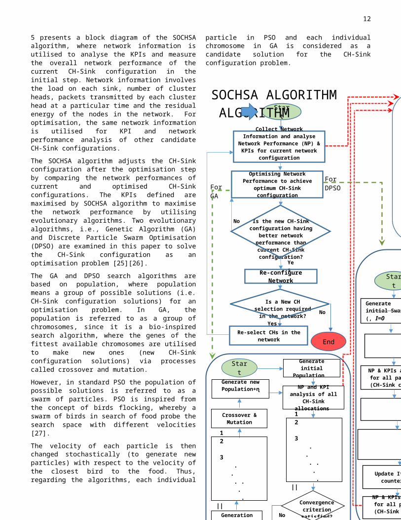
In this section, a centralised SOCHSA algorithm is proposed, which depends on the above intuitive analysis to execute proper CH-Sink configuration. Fig. 5 presents a block diagram of the SOCHSA algorithm, where network information is utilised to analyse the KPIs and measure the overall network performance of the current CH-Sink configuration in the initial step. Network information involves the load on each sink, number of cluster heads, packets transmitted by each cluster head at a particular time and the residual energy of the nodes in the network. For optimisation, the same network information is utilised for KPI and network performance analysis of other candidate CH-Sink configurations.

The SOCHSA algorithm adjusts the CH-Sink configuration after the optimisation step by comparing the network performances of current and optimised CH-Sink configurations. The KPIs defined are maximised by SOCHSA algorithm to maximise the network performance by utilising evolutionary algorithms. Two evolutionary algorithms, i.e., Genetic Algorithm (GA) and Discrete Particle Swarm Optimisation (DPSO) are examined in this paper to solve the CH-Sink configuration as an optimisation problem [25][26].

The GA and DPSO search algorithms are based on population, where population means a group of possible solutions (i.e. CH-Sink configuration solutions) for an optimisation problem. In GA, the population is referred to as a group of chromosomes, since it is a bio-inspired search algorithm, where the genes of the fittest available chromosomes are utilised to make new ones (new CH-Sink configuration solutions) via processes called crossover and mutation.

However, in standard PSO the population of possible solutions is referred to as a swarm of particles. PSO is inspired from the concept of birds flocking, whereby a swarm of birds in search of food probe the search space with different velocities [27].

The velocity of each particle is then changed stochastically (to generate new particles) with respect to the velocity of the closest bird to the food. Thus, regarding the algorithms, each individual particle in PSO and each individual chromosome in GA is considered as a candidate solution for the CH-Sink configuration problem.

No

No

Convergence criterion satisfied?

Yes

No Yes

SOCHSA ALGORITHMStart

Is the new CH-Sink configuration having better network performance than

current CH-Sink configuration?

Collect Network Information and analyse Network Performance (NP)

& KPIs for current network configuration

Optimising Network Performance to achieve optimum CH-Sink

configuration

Is a New CH selection required in the network?

Re-configure Network

For DPSOFor GA

Yes

Re-select CHs in the networkEnd

Start

NP & KPIs analysis for all¿∆∨¿ particles (CH-Sink config.)

Update Iteration counterI=I+1

v jI=iw v j

I−1+c1ε 1 ( pbest jI−x j

I )+c2ε 2 (gbest I−x jI )

x jI +1=x j

I+v jI

gbest I= argmax1≤ j ≤∨∆∨¿F ( pbest j

I )¿

NP & KPIs analysis for all¿∆∨¿ particles (CH-

Sink config:)

pbest jI=r j

I

1 ≤ j≤∨∆∨¿

Generate initial Swarm, (

r1 ,I r2 ,

I …,r|∆|I ¿

1 r1 NP1

2 r2

NP2

3 r3

NP3 . . . . . .

Generate new Populationγ+ɳ

Crossover & Mutation

Generation

1 r1 NP1

2 r2

NP2

3 r3

NP3 . . . . . .

NP and KPI analysis of all |∆|CH-Sink

allocations

Generate initial Population |∆|Start

9

In PSO the velocity is updated for each particle depending on the historical best position experienced (pbest) by the particle itself and the best position experienced by the neighbouring particles, i.e. the global best position (gbest). Standard PSO cannot be applied to the discrete CH-Sink configuration optimisation problem. Therefore, for real valued CH-Sink configuration, a Discrete PSO is proposed in this paper to solve the network performance maximisation problem defined in (20). Both GA and DPSO, as presented in Fig. 5, are explained by the following steps:

Step 1: Initiate random population R0 with a population size of |Δ|. Each candidate solution in the population is B bits, where the number of bits is taken according to the number of CHs in the network at a particular time. For DPSO, initiate the best position for each particle, i.e. pbest j

0=r j0 , where 1≤ j ≤∨∆∨¿ with a random velocity

of v jI for each particle.

Step 2: Determine the fitness value of each chromosome in GA and each particle in DPSO in the initial population using the objective function F (i.e. the NP function defined in (20)). For DPSO, identify the global best position in the swarm/population, i.e. gbest0=¿ F( pbest j

I)1 ≤ j≤∨∆∨ ¿argmax .¿

Step 3: In the case of GA, if the convergence criterion is satisfied, i.e. if the best candidate solution is achieved or the maximum number of generations has passed, then end, or else go to Step 4. However, in the case of DPSO, update the velocity of all the particles in the current population. The velocity update equation is given as:

v jI=iw v j

I−1+c1ε 1 ( pbest jI−x j

I )+c2 ε2(gbest jI− x j

I)1≤ j ≤∨∆∨¿

(21)

where, x jI shows particle j’s current position at iteration

number I. ε 1 and ε 2 are random numbers chosen within the 0-1 range, whereas c1 and c2 are considered to be the acceleration constants that are required to pull the particles towards the best position. The values are chosen for c1and c2 lie within the range 0-5. iw shows the effect of inertia of the preceding particle velocity over the updated particle velocity. The value of iw is altered to achieve global exploration or to expedite the local search. Optimum value selection for iw can assist in both global and local exploration of the search space. Typical values for iw are selected in the range 0-1 [27][28], and in this paper, the value selected is 0.9. Moreover, the updated positions of all particles for the next iteration (I+1) are given as:

x jI +1=( x j

I+v jI)

1≤ j ≤∨∆∨¿(22)

Step 4: In the case of GA, extract a set of |γ | best chromosomes from current population, i.e. R I with a chromosome selection probability of Ps. In the case of DPSO, update the iteration number, i.e. I=I+1.

Step 5: For GA, perform crossover and mutation operations on set γ. The unfeasible solutions (R I−γ) are replaced with newly generated chromosomes μ(i.e. γ+¿ μ¿. For DPSO, if the convergence criterion is satisfied, then end, or else go to Step 6.

Step 6: In the case of GA, repeat all steps from Step 2, whereas, for DPSO, update each particle’s personal best position, i.e.

pbest jI={pbest j

I−1 if F(r jI )≤ F (pbest j

I−1)r j

I if F (r jI)>F ( pbest j

I−1) (23)

Step 7: For DPSO, Update the global best position achieved.

gbest jI={ F ( pbest j

I )1 ≤ j ≤∨Δ∨ ¿argmax if F ( pbest jI)>F (pbest j

I −1)¿ g best jI−1 otherise(24)

Step 8: For DPSO, repeat all steps from Step 1.

VI. COMPUTATIONAL RESULTS AND COMPLEXITY

In this section, the proposed MLCMS is compared with LEACH and M-LEACH, which are commonly deployed algorithms, regarding their performance. Our proposal is found to outperform both of the latter two algorithms about energy conservation and hence, to prolong network life time as shown in Fig.6. The life time of the system refers to the period between its first operation and the demise of the last node. It can be seen that MLCMs lasted for 3716 rounds, while LEACH and M-LEACH achieved 1500 and 1900 rounds, respectively. This is observed in the shape of the graphs, where a steep decrease in LEACH and M-LEACH shows where energy equalisation is attained. When the last node is reached, all nodes are depleted energy resources, leading to this quick decline. On the other hand, MLCMS shows a gradual decrease in the number of alive nodes, which is because energy equalisation is not coordinated and some nodes run out of battery energy much more quickly than others. We can also observe an early jump for LEACH and M-LEACH and sharp decrease as shown in Fig. 6. A jump is seen at the instance when many sensors have depleted their energy resources. Moreover, depending on the definition of the stability, which evaluates the stability of the system regarding on when the first node dead after starting the operation period. It is clear that M-LEACH and LEACH their first node dead before MLCMS, hence has an overwhelming performance in stability.

Generation

10

Two benchmark problems P1 and P2 are considered in this paper, in order to analyse, verify and demonstrate the performance of the SOCHSA algorithm. Both benchmark problems consist of 1,000 sensor nodes randomly distributed in the sensing field.

Fig. 6 Active nodes analysis for MLCMS, M-LEACH and LEACH

Both P1 and P2 are tested at a particular time instance, where 270 CHs are selected in the network. The only difference between the two benchmark problems is that P1 has two sinks, whereas P2 has three. The selection of a different number of sinks in the two problems helps to differentiate between the lifetime of the network regarding average residual energy. An exhaustive search for the optimum CH-Sink configuration is made to compare with the results of SOCHSA algorithm. Also, the performance of K-mean clustering algorithm is tested on P1 and P2 for the sake of comparison [28] as shown in Table II. The Exhaustive Search (ES) algorithm is used to find the optimum CH-Sink configuration. The α and βparameters for (20) are chosen according to a constraint such that α +β ≤ 1. Selecting proper weights for the optimisation function itself is challenging and necessary for proper tuning of evolutionary algorithms. Therefore, an exhaustive search for optimum CH-Sink configuration is performed on P1 with different α and β settings and the overall packet drop is analysed, as shown in Fig.7. The α and β parameters are changed orderly i.e., 0, 0.1,…, 1 subject to the constraint α +β ≤ 1. A much lower packet drop is observed

when the α=0.8 and β=0.2, giving a higher priority to Average residual energy over load fairness index maximisation.

ES performs M N possible CH-Sink configuration solutions for both P1 and P2, where M is the number of sinks and N is

the number of cluster heads in the network, i.e. 2270 and 3270 for P1 and P2, respectively. Note that the initial CH-Sink configuration for both P1 and P2 allows the CHs to transmit to the sinks just above or below their current position, i.e. each sink handles the area above and below it, as the coverage area is divided into four quarters and six sections for P1 and P2, respectively. Fig. 8-10 shows the network performance (fitness function), the average residual energy, and the network load fairness index over 200 generations or iterations for both P1 and P2. The ES algorithm achieves the optimum values shown in the figures. Note that, ES does not depend on generations or iterations. The optimum values are used to demonstrate the improvement achieved by both GA and DPSO at each generation or iteration.

The optimum results achieved from ES are presented in Table II, where the convergence rate for both GA and DPSO is also given. This is defined as the number of times an optimum solution (or the optimum CH-Sink configuration solution) is achieved over the entire number of generations or iterations.

Table II GA, DPSO, AND K-MEAN COMPARISON RESULTS

2 sinks

Network Performance value Convergence Rate Number of iterations CPU time

GA DPSO K-mean GA DPSO GA DPSO GA DPSO K-mean

108.059 108.059 74.8535 0.925 0.94 14 11 0.10 0.09 0.32

3 Sinks 108.1686 108.1686 71.6479 0.86 0.895 28 21 0.48 0.32 0.75

11

00.1

0.20.3

0.40.5

0.60.7

0.80.9

11

0.90.8

0.70.6

0.50.4

0.30.2

0.10

400

200

0

800

600

1200

1000

Pack

et d

rop

Fig .7 Packets Drop with different α and β

In P1, GA converges to the optimum CH-Sink configuration solution after the 14th generation, with a network performance evaluation value of 108.059 (which is optimum), whereas DPSO achieves the optimum network performance value after the 11th iteration. 185 optimum CH-Sink configuration solutions are achieved by GA over 200 generations with a convergence rate of 0.925, while the optimum CH-Sink configuration solutions by DPSO are 188 over 200 iterations with a convergence rate of 0.94. The DPSO converges faster to the optimum CH-Sink configuration solution compared to GA, as shown in Fig. 8 and Table II. The optimum network performance value is achieved after 16x500 (i.e., 16x|Δ|) and 12x500 (i.e. 12x|Δ|) fitness evaluations by GA and DPSO, respectively. However, the ES has to evaluate 2270 possible CH-Sink configuration solutions to find the optimum network performance value, which is too enormous.

For P2, the optimum network performance value achieved by GA and DPSO is after 28th and 21st generations or iterations, respectively. The convergence rates for GA and DPSO are 0.86 and 0.895, respectively, with 172 optimum CH-Sink configurations solutions achieved over 200 generations for GA and 179 for DPSO. Fig. 9 and Fig. 10 show that the average residual energy and the network load fairness index (for both benchmark problems) increase as the GA and DPSO converge to the optimum CH-Sink configuration solution. The average residual energy is improved by 2% when 3 sinks are used compared to 2 sinks. This shows that the use of multiple sinks with the proposed MLCMS protocol for large networks can enhance network lifetime. Since the DPSO outperforms GA. in both the benchmark problems, it is best suitable for the proposed SOCHSA. Note that, the K-mean clustering algorithm takes longer times than GA and DPSO to find a proper CH-Sink configurations allocation in both 2 Sink and 3 sink scenarios, as shown in Table II

This is because both algorithms operate differently. In DPSO, each particle acts as an agent, which updates its velocity in the search space based on social information (i.e. best particle position in the current population or swarm) and global information (i.e. best particle position for all iterations). However, the chromosomes in GA do not act as agents and have no information of other chromosomes in a population. In fact, GA relies on crossover and mutation operations, which could disturb the convergence of the algorithm. Hence, DPSO is suitable for global exploration of the search space.

This paper further demonstrates the performance of MLCMS with and without SOCHSA over 100 nodes as shown in Fig.11 and Fig.12. It is evident from the figures that the lifetime of the network is extended further and the network energy consumption is greatly reduced when the proposed algorithm (SOCHSA) works in tandem with MLCMS protocol.

In Fig. 11, the coefficient of variation of active nodes levels is plotted with respect to round time. MLCMS with SOCHSA shows minimal variation in energy levels, while without SOCHSA, large fluctuations are observed. This indicates that the sensor nodes residual energy level in MLCMS with SOCHSA is significantly improved. Fig. 12 shows the residual energy comparison for MLCMS with and without SOCHSA.

Number of Iterations or Generations0 20 40 60 80 100 120 140 160 180 200

Net

wor

k Pe

rfor

man

ce

106.2

106.4

106.6

106.8

107

107.2

107.4

107.6

107.8

108

108.2

ES, 2 SinksGA, 2 SinksDPSO, 2 SinksES, 3 SinksGA, 3 SinksDPSO, 3 Sinks

Fig. 8 Network performance measurements for GA and DPSO in benchmark problems P1 and P2

12

Number of Iterations or Generations0 20 40 60 80 100 120 140 160 180 200

Ave

rage

Rem

aini

ng E

nerg

y

132

132.5

133

133.5

134

134.5

135

ES, 2 SinksGA, 2 SinksDPSO, 2 SinksES, 3 SinksGA, 3 SinksDPSO, 3 Sinks

Fig. 9 Average residual energy for GA and DPSO in benchmark problems P1 and P2

Number of Iterations or Generations0 20 40 60 80 100 120 140 160 180 200

Loa

d Fa

irnes

s In

dex

0.975

0.98

0.985

0.99

0.995

1

ES, 2 SinksGA, 2 SinksDPSO, 2 SinksES, 3 SinksGA, 3 SinksDPSO, 3 Sinks

Fig. 10 Load fairness index for GA and DPSO in benchmark problems P1 &P2

Fig. 11 Active nodes analysis for MLCMS with and without SOCHSA

This reveals that the lifetime of MLCMS with SOCHSA ends in 4,500 rounds, and after 3,716 rounds without SOCHSA. The proposed architecture can extend the lifetime of wireless

sensor nodes because the MLCMS with 6LoWPAN and SOCHSA provides a sophisticated algorithm aimed to improve the network performance by maximising the load balancing fairness as well as the overall residual energy.

Fig. 12 Residual energy analysis for MLCMS with and without SOCHSA

VII. CONCLUSION

In this paper, an MLCMS protocol to enhance network lifetime along with load balancing solutions have been presented with the aim of improving the network performance of M2M wireless sensor networks. A dynamic CH to sink allocation technique has been investigated. Practical CH-Sink mapping solutions that deliver balanced traffic to the network with high residual energy have been probed. To this end, a self-optimising M2M-WSN algorithm that efficiently deploys network resources has been proposed. The CH-Sink allocation arrangement maximises network performance, by balancing the load across multiple sinks to avoid over-utilisation of the network. Maximising the load fairness index and the average residual energy for the whole M2M network is solved as an optimisation problem. The CH distribution problem is tackled by obtaining an optimal solution with two evolutionary algorithms, namely, GA and DPSO, hosting the SOCHSA algorithm. The performances of both GA and DPSO have been tested and compared to two benchmarking scenarios. DPSO converged notably quicker than GA and also outperformed it in large network scenarios. The MLCMS with SOCHSA algorithm provides significant network benefits regarding network lifetime when compared to MLCMS without SOCHSA. However, the proposed work is limited to clustering WSNs infrastructure. Our future work aims to enable the proposed protocol to support Peer-to-Peer communications to support heterogeneous M2M networks that is foreseen to be in the future of IoT.

REFERENCES[1] M. R. Palattella et al., “Standardized Protocol Stack for the Internet of

(Important) Things,” Commun. Surv. Tutorials, IEEE, vol. 15, no. 3, pp. 1389–1406, 2013.

13

[2] S.-J. Jung and W.-Y. Chung, “Non-Intrusive Healthcare System in Global Machine-to-Machine Networks,” Sensors Journal, IEEE, vol. 13, no. 12, pp. 4824–4830, Dec. 2013.

[3] A. A. Aziz, Y. A. Sekercioglu, P. Fitzpatrick, and M. Ivanovich, “A Survey on Distributed Topology Control Techniques for Extending the Lifetime of Battery Powered Wireless Sensor Networks,” Commun. Surv. Tutorials, IEEE, vol. 15, no. 1, pp. 121–144, 2013.

[4] I. Park, D. Kim, and D. Har, “MAC Achieving Low Latency and Energy Efficiency in Hierarchical M2M Networks With Clustered Nodes,” Sensors Journal, IEEE, vol. 15, no. 3, pp. 1657–1661, Mar. 2015.

[5] M. Alam, R. H. Nielsen, and N. R. Prasad, “The evolution of M2M into IoT,” in Communications and Networking (BlackSeaCom), 2013 First International Black Sea Conference on, 2013, pp. 112–115.

[6] R. A. Khan and A. H. Mir, “Sensor fast proxy mobile IPv6 (SFPMIPv6)-A framework for mobility supported IP-WSN for improving QoS and building IoT,” in Communications and Signal Processing (ICCSP), 2014 International Conference on, 2014, pp. 1593–1598.

[7] F. Ahmed, J. Deng, and O. Tirkkonen, “Self-organizing networks for 5G: Directional cell search in mmW networks,” in Personal, Indoor, and Mobile Radio Communications (PIMRC), 2016 IEEE 27th Annual International Symposium on, 2016, pp. 1–5.

[8] S. Tyagi and N. Kumar, “Journal of Network and Computer Applications A systematic review on clustering and routing techniques based upon LEACH protocol for wireless sensor networks,” J. Netw. Comput. Appl., vol. 36, no. 2, pp. 623–645, 2013.

[9] O. Younis, M. Krunz, and S. Ramasubramanian, “Node clustering in wireless sensor networks: Recent developments and deployment challenges,” IEEE Netw., vol. 20, no. 3, pp. 20–25, 2006.

[10] A. A. Abbasi, “A survey on clustering algorithms for wireless sensor networks,” Comput. Commun., vol. 30, no. 14, pp. 2826–2841, 2007.

[11] C. J. Jiang, W. R. Shi, M. Xiang, and X. L. Tang, “Energy-balanced unequal clustering protocol for wireless sensor networks,” J. China Univ. Posts Telecommun., vol. 17, no. 4, pp. 94–99, 2010.

[12] N. M. A. Latiff, C. C. Tsimenidis, B. S. Sharif, and U. Kingdom, “Energy-Aware Clustering for Wireless Sensor Networks Using Particle Swarm Optimization,” in The 18th Annual IEEE International Sysmposium on Personal, Indoor and Mobile Radio Communications (PIMRC’07), 2007, pp. 5–9.

[13] A. Rahmanian, H. Omranpour, M. Akbari, and K. Raahemifar, “A novel genetic algorithm in LEACH-C routing protocol for sensor networks,” in Electrical and Computer Engineering (CCECE), 2011 24th Canadian Conference on, 2011, pp. 1096–1100.

[14] E. A. Khalil and A. A. Bara’a, “Energy-aware evolutionary routing protocol for dynamic clustering of wireless sensor networks,” Swarm Evol. Comput., vol. 1, no. 4, pp. 195–203, 2011.

[15] W. B. Heinzelman, A. P. Chandrakasan, and H. Balakrishnan, “An application-specific protocol architecture for wireless microsensor networks,” IEEE Trans. Wirel. Commun., vol. 1, no. 4, pp. 660–670, 2002.

[16] P. Kuila, S. K. Gupta, and P. K. Jana, “A novel evolutionary approach for load balanced clustering problem for wireless sensor networks,” Swarm Evol. Comput., vol. 12, pp. 48–56, 2013.

[17] S. Galzarano, C. Savaglio, A. Liotta, and G. Fortino, “Gossiping-Based AODV for Wireless Sensor Networks,” in 2013 IEEE International Conference on Systems, Man, and Cybernetics, 2013, pp. 26–31.

[18] A. Le, J. Loo, A. Lasebae, A. Vinel, Y. Chen, and M. Chai, “The Impact of Rank Attack on Network Topology of Routing Protocol for Low-Power and Lossy Networks,” Sensors Journal, IEEE, vol. 13, no. 10, pp. 3685–3692, Oct. 2013.

[19] X. Wang, “Multicast for 6LoWPAN Wireless Sensor Networks,” Sensors Journal, IEEE, vol. 15, no. 5, pp. 3076–3083, May 2015.

[20] P. Pongle and G. Chavan, “A survey: Attacks on RPL and 6LoWPAN in IoT,” in Pervasive Computing (ICPC), 2015 International Conference on, 2015, pp. 1–6.

[21] R. Roberts and P. Goodwin, “Weight approximations in multiattribute decision models.,” J. Multi-Criteria Decis. Anal., vol. 303, no. June, pp. 291–303, 2002.

[22] F. Farouk, R. Rizk, and F. W. Zaki, “Multi-level stable and energy-efficient clustering protocol in heterogeneous wireless sensor networks,” Wirel. Sens. Syst. IET, vol. 4, no. 4, pp. 159–169, 2014.

[23] V. K. Subhashree, C. Tharini, and M. Swarna Lakshmi, “Modified LEACH: A QoS-aware clustering algorithm for Wireless Sensor Networks,” in Communication and Network Technologies (ICCNT), 2014 International Conference on, 2014, pp. 119–123.

[24] C.-Y. Wan, S. B. Eisenman, A. T. Campbell, and J. Crowcroft, “Overload traffic management for sensor networks,” ACM Trans. Sens. Networks, vol. 3, no. 4, p. 18–es, 2007.

[25] M. D. Vose, The simple genetic algorithm: foundations and theory, vol. 12. MIT press, 1999.

[26] C.-J. Liao, C.-T. Tseng, and P. Luarn, “A discrete version of particle swarm optimization for flowshop scheduling problems,” Comput. Oper. Res., vol. 34, no. 10, pp. 3099–3111, 2007.

[27] J. Kennedy, “Particle swarm optimization,” in Encyclopedia of machine learning, Springer, 2011, pp. 760–766.

[28] J. Vesterstrom and R. Thomsen, “A comparative study of differential evolution, particle swarm optimization, and evolutionary algorithms on numerical benchmark problems,” in Evolutionary Computation, 2004. CEC2004. Congress on, 2004, vol. 2, pp. 1980–1987.

[28] Sasikumar, P., and Sibaram Khara. "K-means clustering in wireless sensor networks." Computational intelligence and communication networks (CICN), 2012 fourth international conference on. IEEE, 2012.