Vibrationdata 1 Unit 4 Random Vibration. Vibrationdata 2 Random Vibration Examples n Turbulent...
33
Vibrationdata Vibrationdata 1 Unit 4 Random Vibration
-
Upload
marylou-tate -
Category
Documents
-
view
227 -
download
0
Transcript of Vibrationdata 1 Unit 4 Random Vibration. Vibrationdata 2 Random Vibration Examples n Turbulent...
VibrationdataVibrationdata
1
Unit 4
Random Vibration
VibrationdataVibrationdata
2
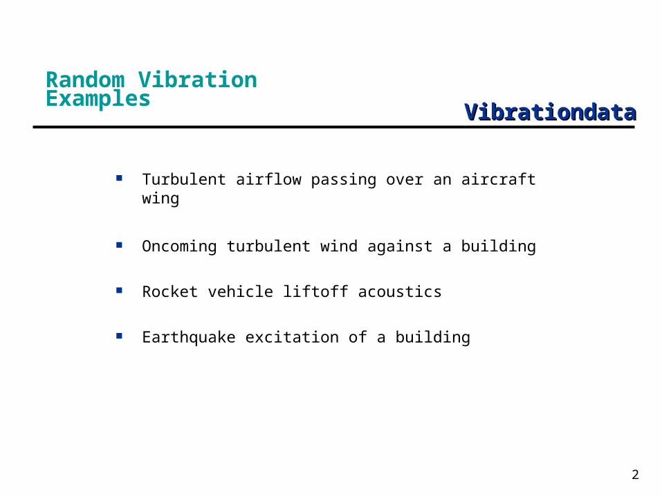
Random Vibration Examples
Turbulent airflow passing over an aircraft wing
Oncoming turbulent wind against a building
Rocket vehicle liftoff acoustics
Earthquake excitation of a building
VibrationdataVibrationdata
3
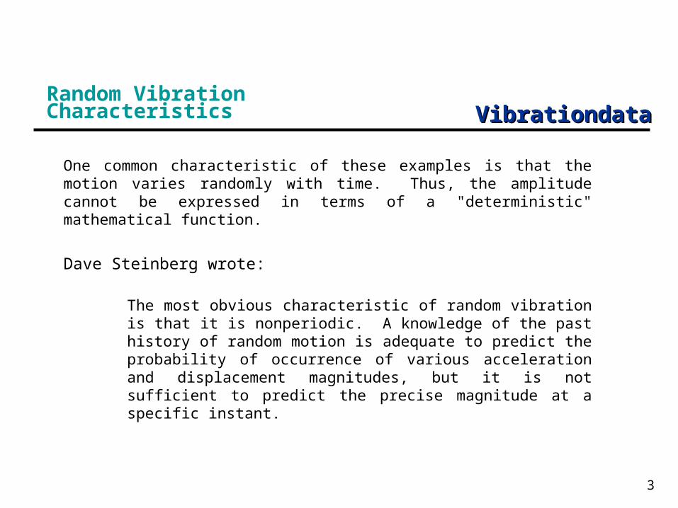
Random Vibration Characteristics
One common characteristic of these examples is that the motion varies randomly with time. Thus, the amplitude cannot be expressed in terms of a "deterministic" mathematical function.
Dave Steinberg wrote:
The most obvious characteristic of random vibration is that it is nonperiodic. A knowledge of the past history of random motion is adequate to predict the probability of occurrence of various acceleration and displacement magnitudes, but it is not sufficient to predict the precise magnitude at a specific instant.
VibrationdataVibrationdata
4
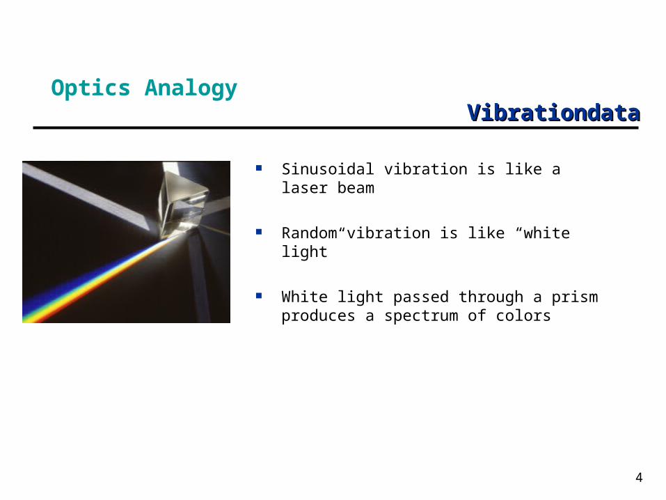
Optics Analogy
Sinusoidal vibration is like a laser beam
Random vibration is like “white light”
White light passed through a prism produces a spectrum of colors
VibrationdataVibrationdata
5
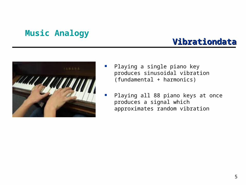
Music Analogy
Playing a single piano key produces sinusoidal vibration (fundamental + harmonics)
Playing all 88 piano keys at once produces a signal which approximates random vibration
VibrationdataVibrationdata
6
Types of Random Vibration
Random vibration can be broadband or narrow band
Random vibration can be stationary or nonstationary
Stationary random vibration is where the key statistical parameters remain constant with each consecutive time segment
Parameters include: mean, standard deviation, histogram, power spectral density, etc.
Shaker table tests can be controlled to be stationary for the test duration
Measured data is usually nonstationary
White noise and pink noise are two special cases of random vibration
VibrationdataVibrationdata
7
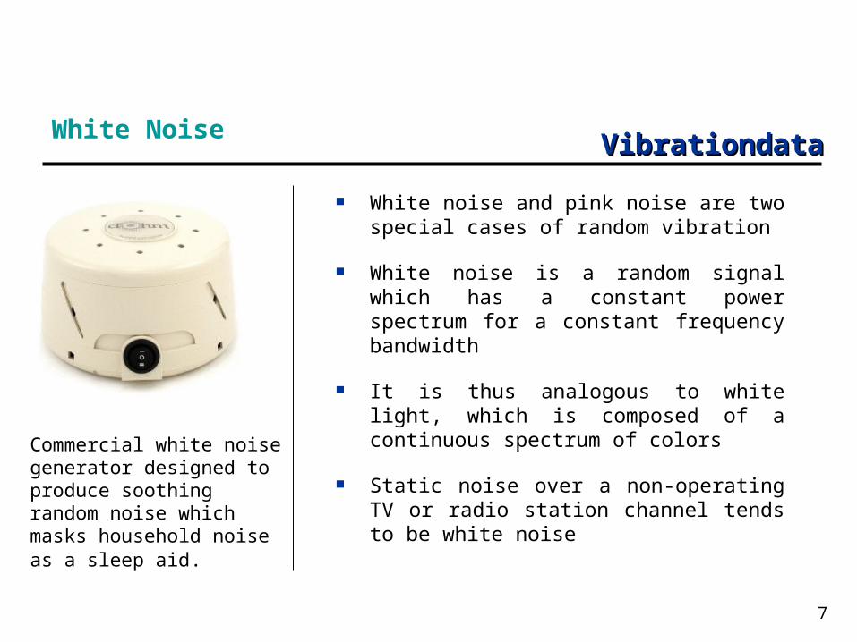
White Noise
White noise and pink noise are two special cases of random vibration
White noise is a random signal which has a constant power spectrum for a constant frequency bandwidth
It is thus analogous to white light, which is composed of a continuous spectrum of colors
Static noise over a non-operating TV or radio station channel tends to be white noise
Commercial white noise generator designed to produce soothing random noise which masks household noise as a sleep aid.
VibrationdataVibrationdata
8
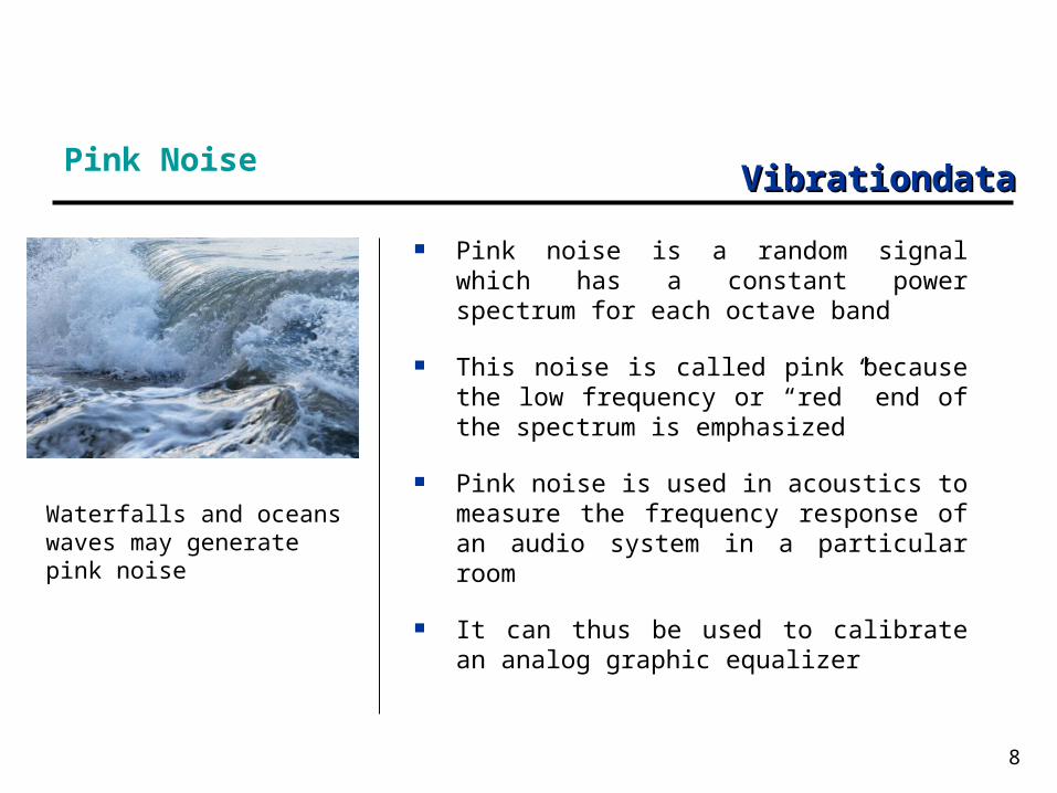
Pink Noise
Pink noise is a random signal which has a constant power spectrum for each octave band
This noise is called pink because the low frequency or “red” end of the spectrum is emphasized
Pink noise is used in acoustics to measure the frequency response of an audio system in a particular room
It can thus be used to calibrate an analog graphic equalizer
Waterfalls and oceans waves may generate pink noise
VibrationdataVibrationdata
9
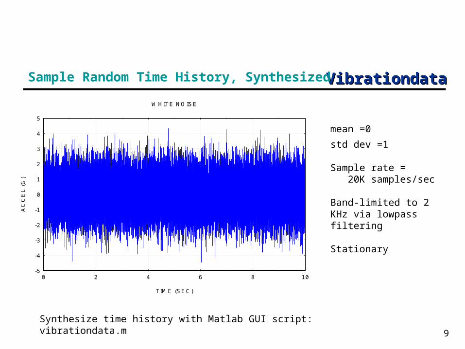
Sample Random Time History, Synthesized
-5
-4
-3
-2
-1
0
1
2
3
4
5
0 2 4 6 8 10
TIME (SEC)
AC
CE
L (G
)
WHITE NOISE
mean =0
std dev =1
Sample rate = 20K samples/sec
Band-limited to 2 KHz via lowpass filtering
Stationary
Synthesize time history with Matlab GUI script: vibrationdata.m
VibrationdataVibrationdata
10
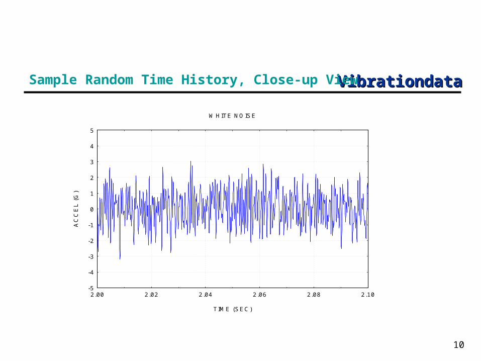
Sample Random Time History, Close-up View
-5
-4
-3
-2
-1
0
1
2
3
4
5
2.00 2.02 2.04 2.06 2.08 2.10
TIME (SEC)
AC
CE
L (G
)
WHITE NOISE
VibrationdataVibrationdata
11
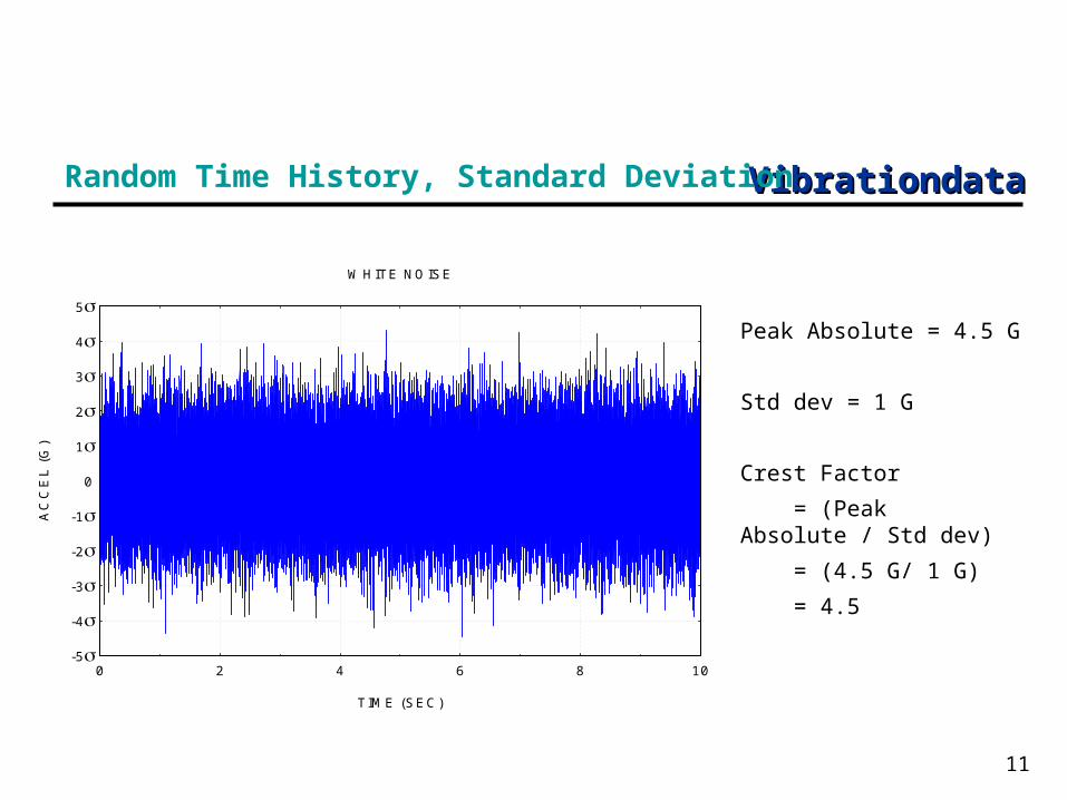
Random Time History, Standard Deviation
-5
-4
-3
-2
-1
0
1
2
3
4
5
0 2 4 6 8 10
TIME (SEC)
AC
CE
L (G
)
WHITE NOISE
Peak Absolute = 4.5 G
Std dev = 1 G
Crest Factor
= (Peak Absolute / Std dev)
= (4.5 G/ 1 G)
= 4.5
VibrationdataVibrationdata
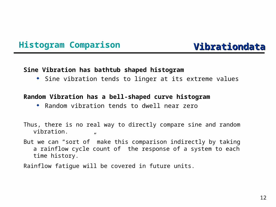
12
Histogram Comparison
Sine Vibration has bathtub shaped histogram Sine vibration tends to linger at its extreme values
Random Vibration has a bell-shaped curve histogram Random vibration tends to dwell near zero
Thus, there is no real way to directly compare sine and random vibration.
But we can “sort of” make this comparison indirectly by taking a rainflow cycle count of the response of a system to each time history.
Rainflow fatigue will be covered in future units.
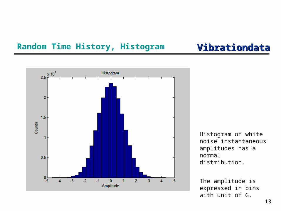
VibrationdataVibrationdata
13
Random Time History, Histogram
Histogram of white noise instantaneous amplitudes has a normal distribution.
The amplitude is expressed in bins with unit of G.
VibrationdataVibrationdata
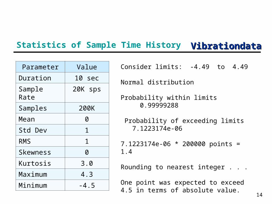
14
Statistics of Sample Time History
Parameter Value
Duration 10 sec
Sample Rate 20K sps
Samples 200K
Mean 0
Std Dev 1
RMS 1
Skewness 0
Kurtosis 3.0
Maximum 4.3
Minimum -4.5
Consider limits: -4.49 to 4.49
Normal distribution
Probability within limits 0.99999288
Probability of exceeding limits 7.1223174e-06
7.1223174e-06 * 200000 points = 1.4
Rounding to nearest integer . . .
One point was expected to exceed 4.5 in terms of absolute value.

VibrationdataVibrationdata
15
RMS and Standard Deviation
= standard deviation
RMS = root-mean-square
[ RMS ] 2 = [ ] 2 + [ mean ]2
RMS = assuming zero mean
VibrationdataVibrationdata
16
Peak and RMS values
Pure sine vibration has a peak value that is 2 times its RMS value
Random vibration has no fixed ratio between its peak and RMS values
Again, the ratio between the absolute peak and RMS values in the previous example is
4.5 G / 1 G = 4.5
VibrationdataVibrationdata
17
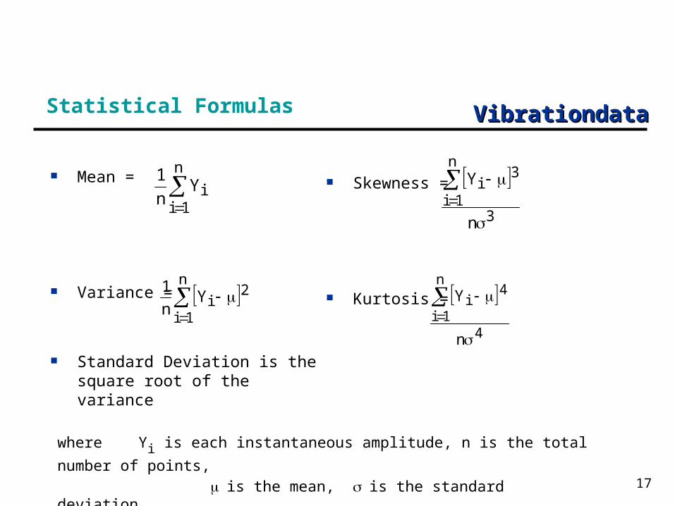
Statistical Formulas
Skewness =
Kurtosis =
4
n
1i
4i
n
Y
3
n
1i
3i
n
Y
Mean =
Variance =
Standard Deviation is the square root of the variance
n
1i
2iY
n
1
n
1iiY
n
1
where Yi is each instantaneous amplitude, n is the total number of points,
is the mean, is the standard deviation
VibrationdataVibrationdata
18
Statistics of Sample Time History
Random vibration is often considered to have a 3 peak for design purposes
Need to differentiate between input and response levels
Response is more important for design purposes, fatigue analysis, etc.
Both input and response can have peaks > 3 even for stationary vibration
VibrationdataVibrationdata
19
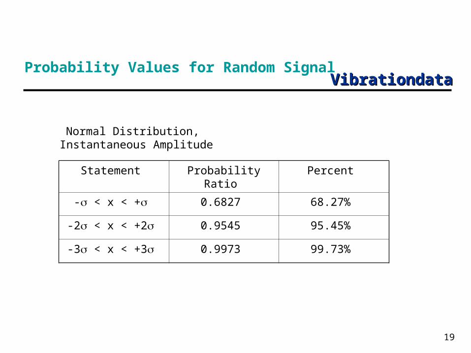
Probability Values for Random Signal
Normal Distribution, Instantaneous Amplitude
Statement Probability Ratio Percent
- < x < + 0.6827 68.27%
-2 < x < +2 0.9545 95.45%
-3 < x < +3 0.9973 99.73%
VibrationdataVibrationdata
20
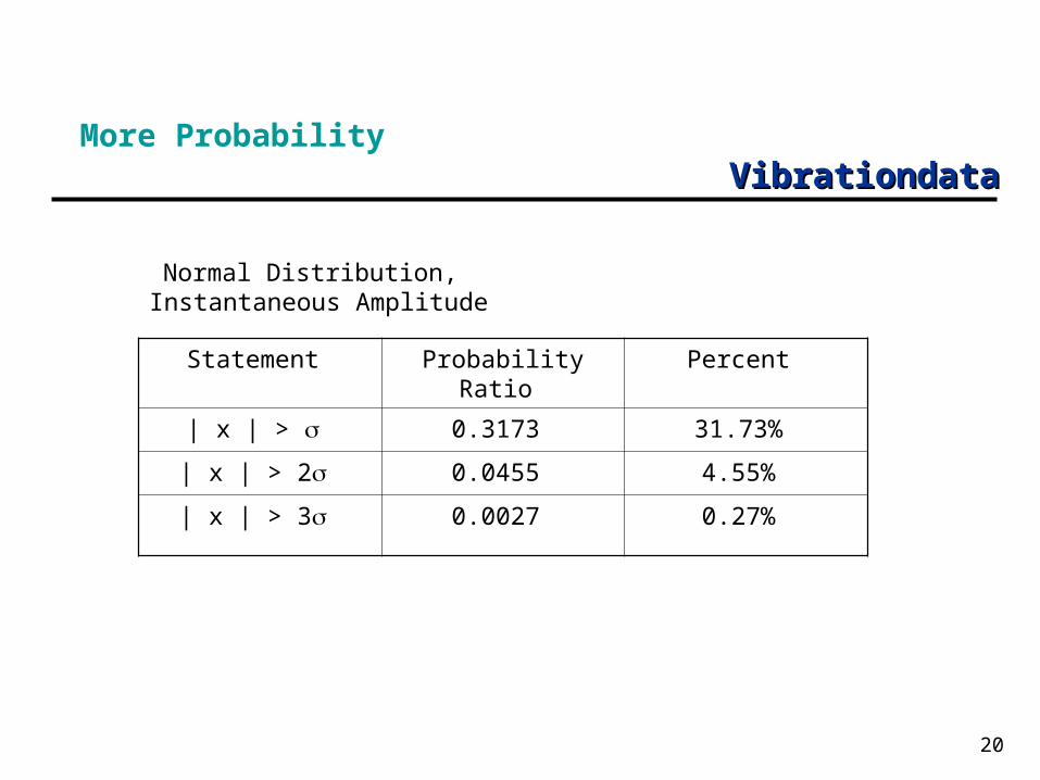
More Probability
Statement Probability Ratio Percent
| x | > 0.3173 31.73%
| x | > 2 0.0455 4.55%
| x | > 3 0.0027 0.27%
Normal Distribution, Instantaneous Amplitude
VibrationdataVibrationdata
21
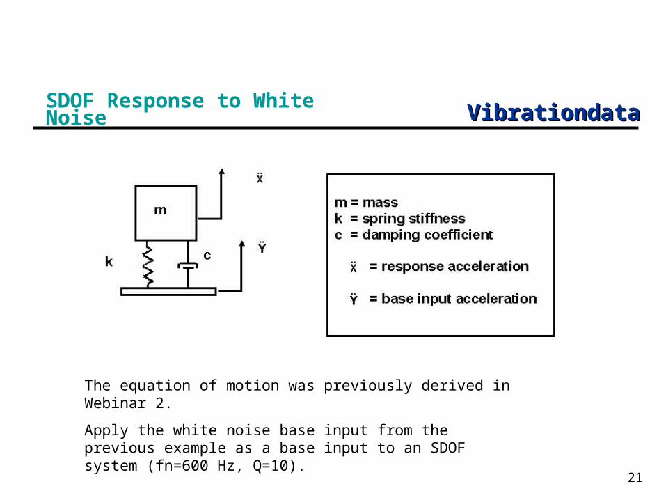
SDOF Response to White Noise
The equation of motion was previously derived in Webinar 2.
Apply the white noise base input from the previous example as a base input to an SDOF system (fn=600 Hz, Q=10).
VibrationdataVibrationdata
22
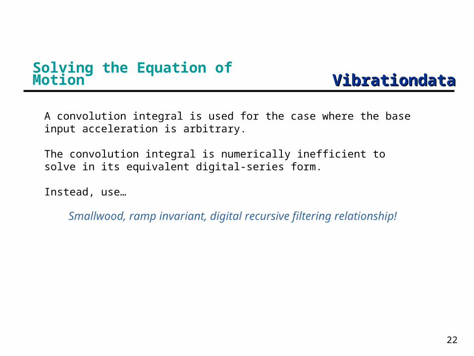
Solving the Equation of Motion
A convolution integral is used for the case where the base input acceleration is arbitrary.
The convolution integral is numerically inefficient to solve in its equivalent digital-series form.
Instead, use…
Smallwood, ramp invariant, digital recursive filtering relationship!
VibrationdataVibrationdata
23
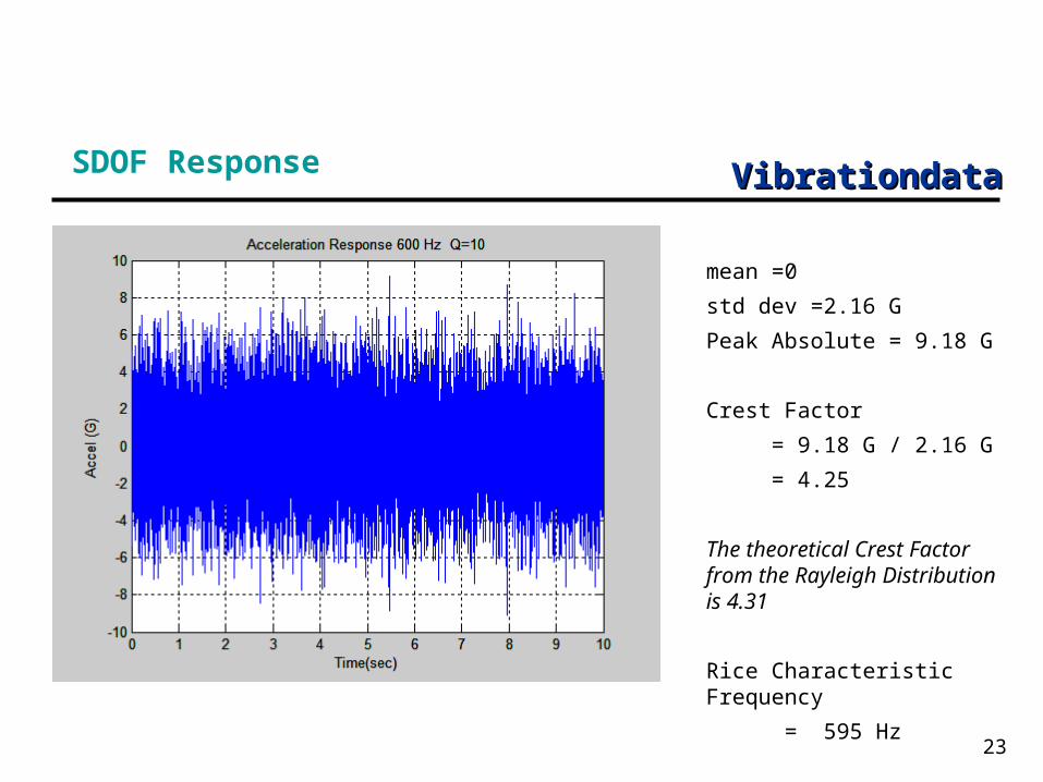
SDOF Response
mean =0
std dev =2.16 G
Peak Absolute = 9.18 G
Crest Factor
= 9.18 G / 2.16 G
= 4.25
The theoretical Crest Factor from the Rayleigh Distribution is 4.31
Rice Characteristic Frequency
= 595 Hz
VibrationdataVibrationdata
24
SDOF Response, Close-up View
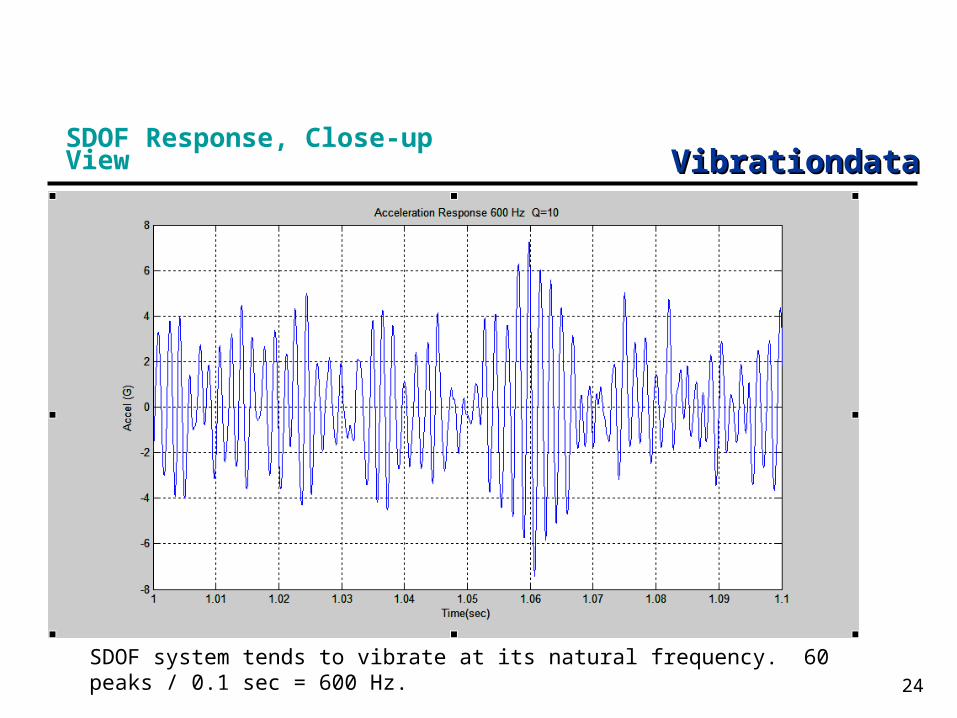
SDOF system tends to vibrate at its natural frequency. 60 peaks / 0.1 sec = 600 Hz.
VibrationdataVibrationdata
25
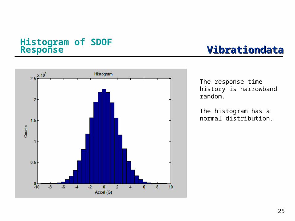
Histogram of SDOF Response
The response time history is narrowband random.
The histogram has a normal distribution.
VibrationdataVibrationdata
26
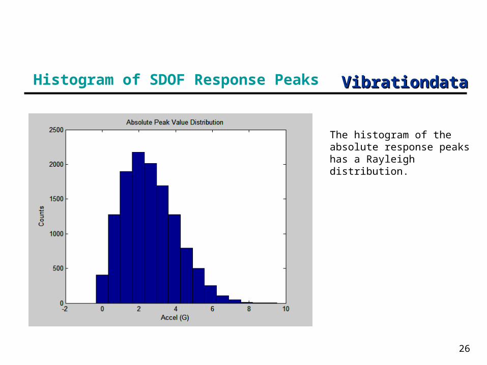
Histogram of SDOF Response Peaks
The histogram of the absolute response peaks has a Rayleigh distribution.
VibrationdataVibrationdata
27
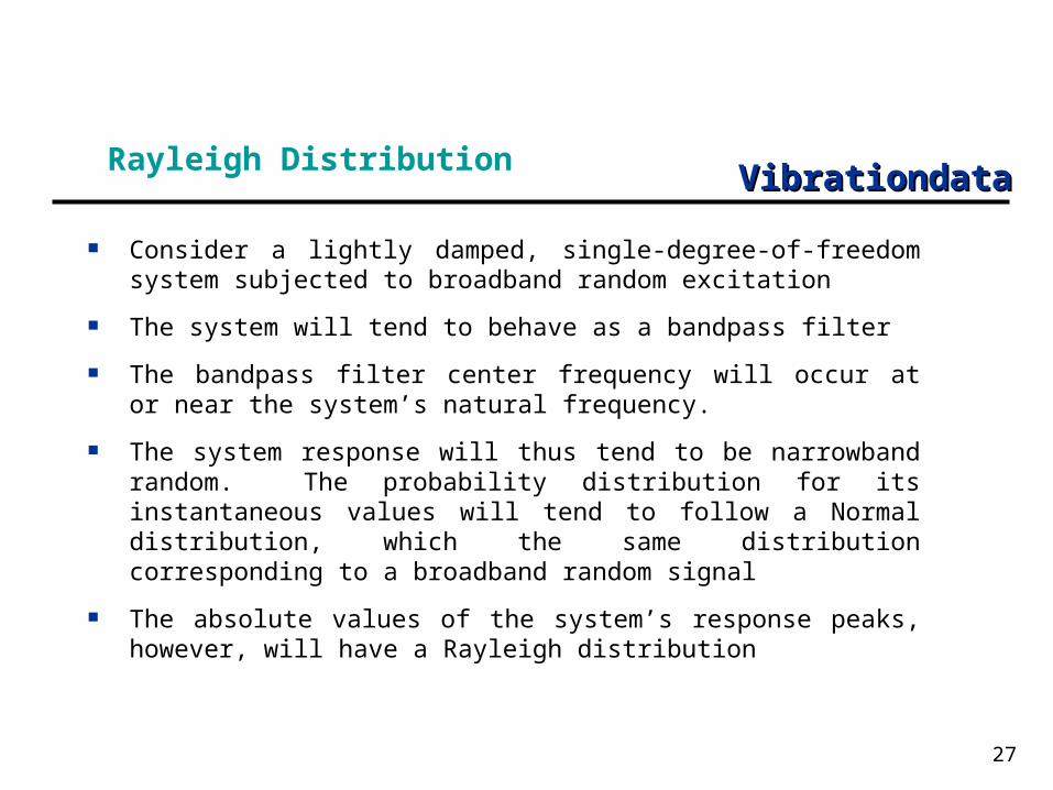
Rayleigh Distribution
Consider a lightly damped, single-degree-of-freedom system subjected to broadband random excitation
The system will tend to behave as a bandpass filter
The bandpass filter center frequency will occur at or near the system’s natural frequency.
The system response will thus tend to be narrowband random. The probability distribution for its instantaneous values will tend to follow a Normal distribution, which the same distribution corresponding to a broadband random signal
The absolute values of the system’s response peaks, however, will have a Rayleigh distribution
VibrationdataVibrationdata
28
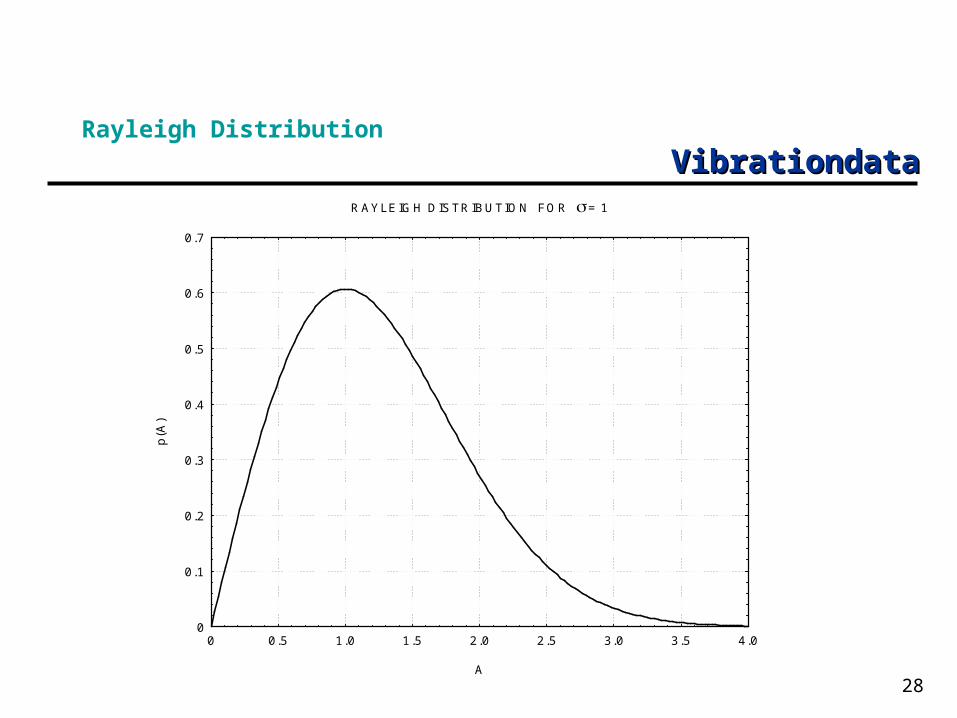
Rayleigh Distribution
0
0.1
0.2
0.3
0.4
0.5
0.6
0.7
0 0.5 1.0 1.5 2.0 2.5 3.0 3.5 4.0
A
p(A
)
RAYLEIGH DISTRIBUTION FOR = 1
VibrationdataVibrationdata
29
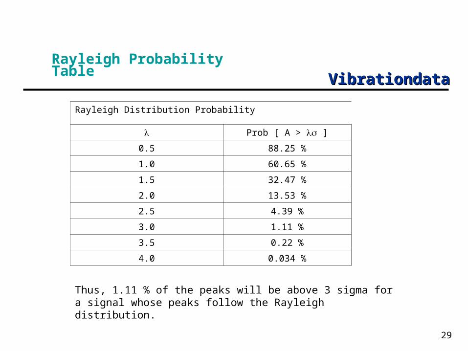
Rayleigh Probability Table
Rayleigh Distribution Probability
Prob [ A > ]
0.5 88.25 %
1.0 60.65 %
1.5 32.47 %
2.0 13.53 %
2.5 4.39 %
3.0 1.11 %
3.5 0.22 %
4.0 0.034 %
Thus, 1.11 % of the peaks will be above 3 sigma for a signal whose peaks follow the Rayleigh distribution.
VibrationdataVibrationdata
30
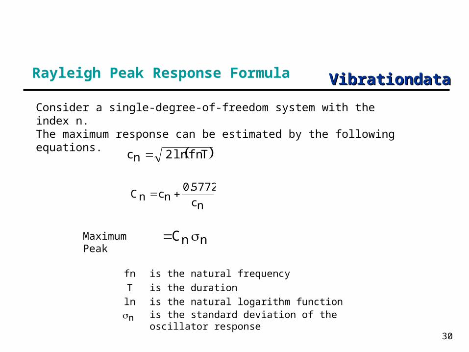
Rayleigh Peak Response Formula
Tfnln2nc
nc
5772.0ncnC
nnC Maximum Peak
fn is the natural frequencyT is the durationln is the natural logarithm function
is the standard deviation of the oscillator responsen
Consider a single-degree-of-freedom system with the index n. The maximum response can be estimated by the following equations.
VibrationdataVibrationdata
31
Unit 4 Exercise 1
Consider an avionics component. It is powered and monitored during a bench test. It passes this "functional test."
Nevertheless, it may have some latent defects such as bad solder joints or bad parts. A decision is made to subject the component to a base excitation test on a shaker table to check for these defects. Which would be a more effective test: sine sweep or random vibration? Why?
Reference: NAVMAT P9492, Section 3.1
VibrationdataVibrationdata
32
Unit 4 Exercise 2
Repeat the pervious examples on your own. Use the vibrationdata.m GUI script.
Generate white noise vibrationdata > Miscellaneous Functions > Generate Signal > white noise
Statistics vibrationdata > Signal Analysis Functions > Statistics
Find probability from Normal distribution curve vibrationdata > Miscellaneous Functions > Statistical Distributions > Normal
VibrationdataVibrationdata
33
Unit 4 Exercise 2 (cont)
SDOF Response vibrationdata > Signal Analysis Functions > SDOF Response to Base Input
Estimated Peak Response from Rayleigh distribution vibrationdata > Miscellaneous Functions > SDOF Response: Peak Sigma