vgam Family Functions for Reduced-Rank Regression and ...
58
vgam Family Functions for Reduced-Rank Regression and Constrained Ordination T. W. Yee November 21, 2006 Beta Version 0.6-5 Thomas W. Yee Department of Statistics, University of Auckland, New Zealand [email protected] http://www.stat.auckland.ac.nz/∼yee Contents 1 Introduction 3 1.1 Some Notation .................................. 4 2 What are RR-VGLMs? 4 2.1 VGLMs and VGAMs ............................... 4 2.2 (Partial) RR-VGLMs ............................... 5 2.3 Why Reduced-Rank Regression? ......................... 6 2.4 Normalizations .................................. 6 2.5 Reduced-Rank Multinomial Logit Model (RR-MLM) .............. 7 3 Summary of RR-VGLM Functions Written 7 3.1 valt.control() ................................ 7 3.2 optim.control() and nlminbcontrol() ................... 8 1
Transcript of vgam Family Functions for Reduced-Rank Regression and ...

vgam Family Functions for Reduced-RankRegression and Constrained Ordination
T. W. Yee
November 21, 2006
Beta Version 0.6-5
© Thomas W. Yee
Department of Statistics,University of Auckland,New [email protected]://www.stat.auckland.ac.nz/∼yee
Contents
1 Introduction 31.1 Some Notation . . . . . . . . . . . . . . . . . . . . . . . . . . . . . . . . . . 4
2 What are RR-VGLMs? 42.1 VGLMs and VGAMs . . . . . . . . . . . . . . . . . . . . . . . . . . . . . . . 42.2 (Partial) RR-VGLMs . . . . . . . . . . . . . . . . . . . . . . . . . . . . . . . 52.3 Why Reduced-Rank Regression? . . . . . . . . . . . . . . . . . . . . . . . . . 62.4 Normalizations . . . . . . . . . . . . . . . . . . . . . . . . . . . . . . . . . . 62.5 Reduced-Rank Multinomial Logit Model (RR-MLM) . . . . . . . . . . . . . . 7
3 Summary of RR-VGLM Functions Written 73.1 valt.control() . . . . . . . . . . . . . . . . . . . . . . . . . . . . . . . . 73.2 optim.control() and nlminbcontrol() . . . . . . . . . . . . . . . . . . . 8
1

4 Other RR-VGLM Topics 84.1 Normalizations . . . . . . . . . . . . . . . . . . . . . . . . . . . . . . . . . . 84.2 Output . . . . . . . . . . . . . . . . . . . . . . . . . . . . . . . . . . . . . . 84.3 Implementation Details . . . . . . . . . . . . . . . . . . . . . . . . . . . . . 94.4 Convergence . . . . . . . . . . . . . . . . . . . . . . . . . . . . . . . . . . . 94.5 Latent Variable Plots and Biplots . . . . . . . . . . . . . . . . . . . . . . . . 94.6 Miscellaneous Notes . . . . . . . . . . . . . . . . . . . . . . . . . . . . . . . 9
5 RR-VGLM Tutorial Examples 105.1 Stereotype model . . . . . . . . . . . . . . . . . . . . . . . . . . . . . . . . 105.2 Goodman’s RC Association Model . . . . . . . . . . . . . . . . . . . . . . . . 155.3 Some advice . . . . . . . . . . . . . . . . . . . . . . . . . . . . . . . . . . . 215.4 A Goodman’s RC Numerical Example . . . . . . . . . . . . . . . . . . . . . . 215.5 Other Reduced-Rank Regression work . . . . . . . . . . . . . . . . . . . . . . 25
6 Quadratic RR-VGLMs for CQO 266.1 Normalizations for QRR-VGLMs . . . . . . . . . . . . . . . . . . . . . . . . . 276.2 Fitting QRR-VGLMs with vgam . . . . . . . . . . . . . . . . . . . . . . . . 27
6.2.1 Initial Values . . . . . . . . . . . . . . . . . . . . . . . . . . . . . . . 286.2.2 Some Tricks and Advice . . . . . . . . . . . . . . . . . . . . . . . . . 286.2.3 Timings . . . . . . . . . . . . . . . . . . . . . . . . . . . . . . . . . 306.2.4 Arguments ITolerances and EqualTolerances . . . . . . . . . . . 316.2.5 The isdlv argument . . . . . . . . . . . . . . . . . . . . . . . . . . 31
6.3 After Fitting a QRR-VGLM . . . . . . . . . . . . . . . . . . . . . . . . . . . 346.3.1 The Three Cases . . . . . . . . . . . . . . . . . . . . . . . . . . . . . 346.3.2 Latent variable plots . . . . . . . . . . . . . . . . . . . . . . . . . . . 356.3.3 Perspective Plots . . . . . . . . . . . . . . . . . . . . . . . . . . . . . 356.3.4 Trajectory plots . . . . . . . . . . . . . . . . . . . . . . . . . . . . . 36
6.4 Negative Binomial and Gamma Data . . . . . . . . . . . . . . . . . . . . . . 376.5 A Summary . . . . . . . . . . . . . . . . . . . . . . . . . . . . . . . . . . . 376.6 CQO Examples . . . . . . . . . . . . . . . . . . . . . . . . . . . . . . . . . . 386.7 Example 1 . . . . . . . . . . . . . . . . . . . . . . . . . . . . . . . . . . . . 386.8 Example 2 . . . . . . . . . . . . . . . . . . . . . . . . . . . . . . . . . . . . 416.9 Example 3 . . . . . . . . . . . . . . . . . . . . . . . . . . . . . . . . . . . . 446.10 Calibration . . . . . . . . . . . . . . . . . . . . . . . . . . . . . . . . . . . . 456.11 Miscellaneous Notes . . . . . . . . . . . . . . . . . . . . . . . . . . . . . . . 45
7 Unconstrained Quadratic Ordination (UQO) 46
8 Constrained Additive Ordination (CAO) 478.1 Controlling Function Flexibility . . . . . . . . . . . . . . . . . . . . . . . . . 478.2 CAO Example . . . . . . . . . . . . . . . . . . . . . . . . . . . . . . . . . . 48
2

9 Ordinal Ordination 499.1 Example . . . . . . . . . . . . . . . . . . . . . . . . . . . . . . . . . . . . . 51
10 Not Yet Been Implemented 55
Exercises 55
References 56
[Important note: This document and code is not yet finished, but should be completed oneday . . . ]
1 Introduction
This document describes three classes of models that are variants or extensions of the VGLM andVGAM classes. These variants are summarized in Table 1. Their primary defining characteristicis that they operate on latent variables ν. The word “latent variable” has several shades ofmeaning in statistics but here it is defined as a linear combination of some explanatory variablesx2, i.e., ν = CT x2 for some matrix of coefficients C is a vector of latent variables. Thisdocument does not explain all the technicalities behind each model in Table 1, therefore theinterested reader is referred to the primary references for further details. Instead, this documentfocusses on the practical aspects of using the vgam package to fit the models.
The three central functions in this document are quite similar to vglm() but with additionalfeatures. The vglm() function is similar in spirit to glm(), which is described in Chambers andHastie (1993). The document “vgam Family Functions for Categorical Data” is also relevantto this one, as regression models for categorical responses naturally produce a large number ofparameters, therefore are good candidates for reduced-rank modelling.
Table 1: A summary of the models described in this document. The latent variables ν =CT x2, or ν = cT x2 if R = 1. These models compare with VGLMs where η = BT
1 x1+BT2 x2.
Abbreviations: A = additive, C = constrained (preferred) or canonical, L = linear, O =ordination, Q = quadratic, RR = reduced-rank, VGLM = vector generalized linear model.
η Model Purpose S function Reference
BT1 x1 + Aν RR-VGLM CLO rrvglm() Yee and Hastie (2003)
BT1 x1 + Aν +
M∑j=1
(νTDjν)ej QRR-VGLM CQO cqo() Yee (2004)
BT1 x1 +
R∑r=1
f r(νr) RR-VGAM CAO cao() Yee (2006a)
3

1.1 Some Notation
Our data set comprises of the matrices Y and X which are n× q and n× p respectively. Y isthe response and X is explanatory. There are n individuals (e.g., people or sites) under study,and i is used to index them. For each individual, a q-dimensional response vector y (q ≥ 1) anda p-dimensional covariate vector x = (x1, . . . , xp)
T is observed, e.g., p environmental variables.It is convenient to partition x into (xT
1 , xT2 )T later. In this document, often q = M = S, where
S is the total number of species. The number of linear/additive predictors is always M . Theindex s = 1, . . . , S indexes species.
We have ν = CT x2 = (ν1, . . . , νR)T . If R = 1 then we sometimes write ν = cT x2. Formodels with an intercept term it is assumed that x1 = 1, i.e., that of the first element ofx. The vector ei is a vector of zeros but with a 1 in the ith position. The dimension of thereduced-rank regression is called the rank, R, and is usually 1 or 2 here. It is the number ofaxes in an ordination. The matrix C contains the canonical (or constrained) coefficients andare highly interpretable. They are sometimes called the weights or loadings.
2 What are RR-VGLMs?
To find out what RR-VGLMs are, we need to recall what VGLMs and VGAMs are.
2.1 VGLMs and VGAMs
VGLMs are defined as a model for which the conditional distribution of Y given x is of theform
f(y|x;B) = h(y, η1, . . . , ηM , φ)
for some known function h(·), where B = (β1 β2 · · · βM) is p×M , φ is a dispersion parameter,and
ηj = ηj(x) = βTj x = β(j)1 x1 + · · ·+ β(j)p xp (1)
is the jth linear predictor. GLMs (McCullagh and Nelder, 1989) are a special case having onlyM = 1 linear predictor, and frequently M does not coincide with the dimension of y. We have
η(xi) =
η1(xi)
...ηM(xi)
= ηi = BT xi. (2)
Let η0 = (β(1)1, · · · , β(M)1)T be the vector of intercepts.
VGAMs provide additive-model extensions to VGLMs, that is, (1) is generalized to
ηj(x) = β(j)1 + f(j)2(x2) + · · ·+ f(j)p(xp), j = 1, . . . ,M, (3)
a sum of smooth functions of the individual covariates, just as with ordinary GAMs (Hastie andTibshirani, 1990). The ηj in (3) are referred to as additive predictors. For identifiability, eachcomponent function is centered, i.e., E[f(j)k] = 0.
In practice, it is very useful to consider constraints-on-the-functions. For VGAMs, we have
η(x) = η0 + f 2(x2) + · · ·+ f p(xp)
= H1 β∗1 + H2 f ∗
2(x2) + · · ·+ Hp f ∗p(xp) (4)
4

where H1,H2, . . . ,Hp are known full-column rank constraint matrices, f ∗k is a vector containing
a possibly reduced set of component functions and β∗1 is a vector of unknown intercepts. With
no constraints at all, H1 = H2 = · · · = Hp = IM and β∗1 = η0. Like the fk, the f ∗
k arecentered. For VGLMs, the fk are linear so that
BT =(H1β
∗1 · · · Hpβ
∗p
). (5)
VGLMs are usually estimated by maximum likelihood estimation by Fisher scoring or Newton-Raphson.
2.2 (Partial) RR-VGLMs
Partition x into (xT1 , xT
2 )T and B = (BT1 BT
2 )T . In general, B is a dense matrix of full rank, i.e.,rank min(M, p). Thus there are M × p regression coefficients to estimate. For some data setsboth M and p are“too” large. For example, in a classification problem of the letters“A”to“Z”and“0”to“9”using a 16× 16 grey-scale character digitization, we have M + 1 = 26 + 10 = 36and p = 1 + 162 = 257 in a multinomial logit model. Then there would be M × p = 9252coefficients! Unless the data set was huge this would mean that the standard errors of eachcoefficient would be very large and some simplification would be necessary. Additionally, fittingthe model in the first case would require a super computer because of massive memory andcomputational requirements.
One solution is based on a simple and elegant idea: replace B2 by a reduced-rank regression.This will cut down the number of regression coefficients enormously if the rank R is kept low.Ideally, the problem can be reduced down to one or two dimensions—a successful application ofdimension reduction—and therefore can be plotted. The reduced-rank regression is applied toB2 because we want to make provision for some variables x1 that we want to leave alone. Thismeans B1 remains unchanged. In practice, we often let x1 = 1 for the intercept term only.
The idea of reduced-rank regression was first proposed by Anderson (1951) and since thenalmost all applications of it has been to continuous responses (normal errors)—this is one reasonwhy reduced-rank regression has never become as popular as it should be. In more detail, thenew class, called RR-VGLMs has
η = BT1 x1 + ACT x2 = BT
1 x1 + Aν, (6)
where C = (c(1) c(2) · · · c(R)) is p2 × R, A = (a(1) a(2) · · ·a(R)) = (a1, . . . ,aM)T is M × R.Both A and C are of full-column rank. The effect is that it replaces the dense matrix B2 bythe product of two thin matrices C and AT . Of course, R ≤ min(M, p2) but ideally we wantR min(M, p2). One can think of (6) as a reduced-rank regression of the coefficients of x2
after having adjusted for the variables in x1.Strictly speaking, we call models given by (6) partial RR-VGLMs because only a part of the
regressors have a reduced-rank representation. But we drop the “partial” for convenience. Letdim(x1) = p1 and dim(x2) = p2 so that p1+p2 = p. To distinguish between variables belongingto x1 and x2, the argument Norrr receives a formula with terms that are left untouched byreduced-rank regression, i.e., those for x1. By default, Norrr ∼ 1 for x1 = 1. Here’s anotherexample.
rrvglm(y ~ x2 + x3 + x4 + x5, family = famfun(parallel = TRUE ~ x2 - 1),
Norrr = ~ x2 + x3)
This means that only variables x4 and x5 are represented by reduced-rank regression; that is,x2 = (X4, X5)
T , and x1 = (1, X2, X3)T are left alone. The variable X2 receives a parallelism
constraint.
5

2.3 Why Reduced-Rank Regression?
There are a number of reasons why reduced-rank regression is a good idea:
1. If R min(M, p2) then a more parsimonious model results. The resulting number ofparameters is often much less than the full model (the difference is (M − R)(p2 − R),which is substantial when R min(M, p2)).
2. The reduced-rank approximation provides a vehicle for a low dimensional view of the data,e.g., the biplot. This is illustrated later.
3. It allows for a flexible nonparametric generalization—called RR-VGAMs. These are de-scribed in Section 8.
4. It is readily interpretable. One can think of ν as a vector of R latent variables—linearcombinations of the original predictor variables that give more explanatory power. Theyoften can be thought of as a proxy for some underlying variable behind the mechanismof the process generating the data. For some models, such as the cumulative logit model(McCullagh, 1980), this argument is natural and well-known. In fields such as plantecology the idea is an important one.
Unfortunately, much of the standard theory of reduced-rank regression (see, for example, Reinseland Velu (1998)) and its ramifications are not applicable to RR-VGLMs in general. This is dueto technical reasons. Another complication in inference of RR-VGLMs is that the solution to alower rank problem is not nested within a higher rank problem.
2.4 Normalizations
The factorization (6) is not unique because ηi = BT1 x1 + AMM−1 νi for any nonsingular
matrix M. The following lists some common uniqueness constraints.
1. Restrict A to the form
A =
(IR
A
), say. (7)
(Actually, it may be necessary to represent IR in rows other than the first R.) This isused when derivatives are used to fit the model. This type of constraint is called a Cornerconstraint and corresponds to Corner=TRUE in rrvglm().
2. Another normalization of A, which makes direct comparisons with other statistical meth-ods possible, is based on the singular value decomposition (SVD)
ACT = (UDα)(D1−αVT ) (8)
for some specified 0 ≤ α ≤ 1. For the alternating method of estimation, α = 12
isthe default as it scales both sides symmetrically. The parameter α is Alpha=0.5 inrrvglm.control().
3. It is often possible to choose M so that Var(M−1 ν) is diagonal and its trace is 1.
4. For the stereotype model described in the next section, we could choose M so thatthe columns of C, c(r), r = 1, . . . , R, are orthogonal with respect to the within-groupcovariance matrix W—this type of normalization is similar to linear discriminant analysis.
5. Sometimes we want to choose M so that the latent variables are uncorrelated, i.e.,Var(νi) is diagonal.
6

2.5 Reduced-Rank Multinomial Logit Model (RR-MLM)
The multinomial logit model (MLM) is a popular regression model for categorical data. Itappears under other names, such as the multiple logistic regression model or polytomous logisticregression model. The MLM is given by
pj = P (Y = j|x) =expηj(x)
M+1∑`=1
expη`(x), j = 1, . . . ,M + 1,
where ηj(x) = βTj x. and yi is a (M + 1)-vector of counts for a categorical response variable
taking levels 1, 2, . . . ,M +1. The MLM is used for a nominal response and is particularly usefulfor exploring how the relative chances of falling into the response categories depend upon thecovariates: pj(x)/pk(x) = exp ηj(x)− ηk(x). Identifiability constraints, e.g., ηM+1(x) ≡ 0,are required by the model. This implies
log
(pj
pM+1
)= ηj, j = 1, . . . ,M.
vgam fits the multinomial logit model using the family function multinomial(). It uses thelast column of the response matrix as baseline, or if the response is a factor, the last level. Thespecial case of M = 1 corresponds to logistic regression. For further details, see the article“vgam Family Functions for Categorical Data”.
The reduced-rank version of the MLM, the RR-MLM, was proposed by Anderson (1984). Hecalled it the stereotype model. Note that Anderson (1984) defined his rank-1 stereotype modelto have ordered constraints on the parameters of the A matrix; vgam ignores this as it wouldbe very difficult to estimate the model with such a constraint. Greenland (1994) attempted topopularize the 1-dimensional stereotype model.
A typical RR-MLM can be fitted like
fit = rrvglm(cbind(y1,y2,y3,y4) ~ x2 + x3 + x4 + x5, family = multinomial,
data = mydata, Norrr = ~ 1 + x2, Rank = 2)
3 Summary of RR-VGLM Functions Written
The function rrvglm() should operate on all vgam family functions with M > 2, althoughreduced-rank regression does not make sense for many of them. It returns an object with class"rrvglm" which is, not surprisingly, related to a "vglm" object.
Table 2 gives the current list of S functions that have been written. The function rrvglm.control()is the control function for rrvglm(). It calls either valt.control(), optim.control() forR or nlminbcontrol() for S-PLUS, which are the control functions of valt(), optim(), andnlminb().
Table 5 lists generic functions which are also applicable to RR-VGLMs.
3.1 valt.control()
valt() implements the alternating algorithm. This algorithm (see (6)) fixes C and solves forA and B1, and then fixes C and solves for A and B1; this can be iterated until convergence.The most important arguments to valt.control() are Linesearch and Maxit.
7
3.2 optim.control() and nlminbcontrol()
In R, optim() is used for the derivative-based algorithm, while in S-PLUS, nlminb() is used.The functions optim.control() and nlminbcontrol() pass on parameters to the optimizingfunctions.
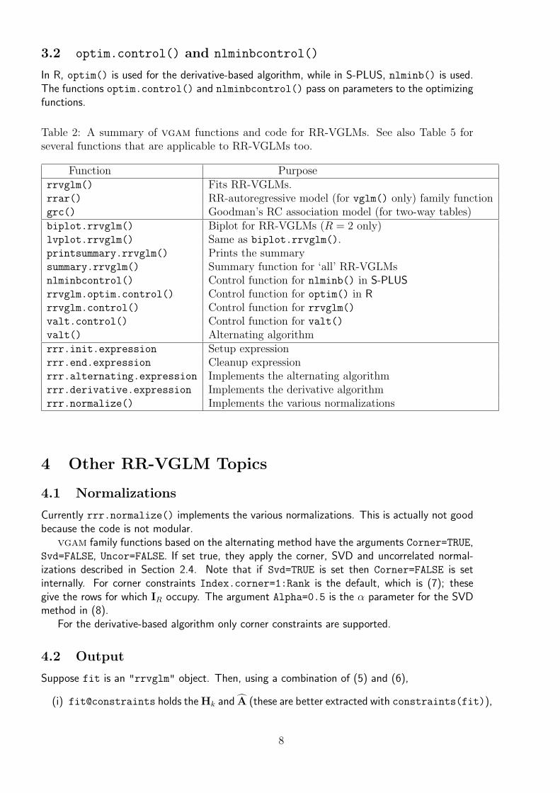
Table 2: A summary of vgam functions and code for RR-VGLMs. See also Table 5 forseveral functions that are applicable to RR-VGLMs too.
Function Purposerrvglm() Fits RR-VGLMs.rrar() RR-autoregressive model (for vglm() only) family functiongrc() Goodman’s RC association model (for two-way tables)biplot.rrvglm() Biplot for RR-VGLMs (R = 2 only)lvplot.rrvglm() Same as biplot.rrvglm().printsummary.rrvglm() Prints the summarysummary.rrvglm() Summary function for ‘all’ RR-VGLMsnlminbcontrol() Control function for nlminb() in S-PLUSrrvglm.optim.control() Control function for optim() in Rrrvglm.control() Control function for rrvglm()valt.control() Control function for valt()valt() Alternating algorithmrrr.init.expression Setup expressionrrr.end.expression Cleanup expressionrrr.alternating.expression Implements the alternating algorithmrrr.derivative.expression Implements the derivative algorithmrrr.normalize() Implements the various normalizations
4 Other RR-VGLM Topics
4.1 Normalizations
Currently rrr.normalize() implements the various normalizations. This is actually not goodbecause the code is not modular.
vgam family functions based on the alternating method have the arguments Corner=TRUE,Svd=FALSE, Uncor=FALSE. If set true, they apply the corner, SVD and uncorrelated normal-izations described in Section 2.4. Note that if Svd=TRUE is set then Corner=FALSE is setinternally. For corner constraints Index.corner=1:Rank is the default, which is (7); thesegive the rows for which IR occupy. The argument Alpha=0.5 is the α parameter for the SVDmethod in (8).
For the derivative-based algorithm only corner constraints are supported.
4.2 Output
Suppose fit is an "rrvglm" object. Then, using a combination of (5) and (6),
(i) fit@constraints holds the Hk and A (these are better extracted with constraints(fit)),
8
(ii) coef(fit) holds the β∗k and vec(C
T),
(iii) coef(fit, matrix=TRUE) is the estimate of B = (BT1 ACT )T ,
(iv) Coef(fit) returns A, C, B1 etc.
The function lv.rrvglm() returns a n × R matrix of latent variables with the ith rowequalling νT
i . These are plotted in lvplot.rrvglm() (rank-2 only), which is equivalent tobiplot.rrvglm().
4.3 Implementation Details
The S expression rrr.init.expression contains essential code that is inserted into vglm.fit()to give rrvglm.fit(). Furthermore, one of rrr.alternating.expression and rrr.derivative.expressionis also used: these perform, e.g., an alternating algorithm iteration between successive Newton-Raphson/Fisher scoring iterations.
The function valt.control() allows a RR-VGLM family function to have arguments thataffect valt(). It has the same type of effect that vglm.control() has on vglm(). Sim-ilarly, rrvglm.optim.control() and nlminbcontrol() for the derivative based algorithm.Arguments usually start with an uppercase letter to avoid conflict with the control parametersassociated with those of vglm().
4.4 Convergence
The alternating algorithm can be very slow at converging but vgam allows a line searchin the alternating method which may improve convergence substantially. It is invoked byLinesearch=TRUE.
Unknown elements in C are chosen randomly using rnorm(). One should use set.seed()
before calling rrvglm() to control this if reproducibility is required.
4.5 Latent Variable Plots and Biplots
Biplots are available for RR-VGLMs and provide a graphical summary of the rank-2 approxi-mation to B2. These are based on Equation (6), and show that the k-j element of B2 is theinner-product of the kth row of C and the jth row of A. The rows of C are usually repre-sented by arrows, and the rows of A by points (labelled by object@misc$predictors.names).Currently, lvplot.rrvglm() is equivalent to biplot.rrvglm().
If fit2 is a rank-2 RR-VGLM, then lvplot(fit2) will produce a scatter plot of the fittedlatent variables νi2 versus νi1 (see (6)). A convex hull can be overlaid on each group. Bydefault, all the observations belong to one group.
4.6 Miscellaneous Notes
1. summary.rrvglm() computes asymptotic standard errors. If the matrix @cov.unscaledis not positive-definite (this would indicate an ill-posed model, e.g., one where the in-tercepts are part of x2 rather than x1), then a warning is given. In such cases the usershould try
(a) numerical=TRUE to use numerical derivatives,
(b) fitting another model,
9

(c) increasing the rank.
Alternatively, there are the options omit13 and kill.all in summary.rrvglm() thatallow an ‘inferior’ @cov.unscaled to be returned, for example, one where A is fixed orone where C is fixed. Then the standard errors are too small.
2. summary.rrvglm() only works with corner constraints (7), i.e., if object@control$Corner=TRUE.In the output, the elements of A in (7) come first. They are labelled with the prefix"I(lv.mat)" or something similar. The elements are enumerated going down each col-umn starting from the first column, i.e., vec(A). Then comes the fitted coefficients β
∗k
corresponding to B1, followed by vec(CT ). Actually, B1 and vec(CT ) are intermingled,depending on the order of the original formula.
3. φ is estimated if summary(..., dispersion=0) is invoked. Then
φ =1
nM − p∗
n∑i=1
(zi − B
T
1 x1i − A CTx2i
)TWi
(zi − B
T
1 x1i − A CTx2i
)(9)
where p∗ = dim(β∗T1 , . . . , β
∗Tp1
, vec(A)T )T is the total number of parameters to be esti-mated.
4. For an example of a reduced-rank autoregressive model for time-series data see Ahn andReinsel (1988).
5 RR-VGLM Tutorial Examples
In this section we illustrate some of the models available.
5.1 Stereotype model
The data frame car.all is available in S-PLUS (type data(car.all) in R) We first preprocessthe data.
> data(car.all)
> cars = car.all
> y = cars[["Country"]]
> cars = cars[y == "USA" | y == "Japan" | y == "Germany" |
+ y == "Japan/USA", ]
> cars = cars[, c("Country", "Length", "Width", "Weight",
+ "HP", "Disp.", "Price")]
> cars = na.omit(cars)
> cars[, -1] = scale(cars[, -1])
> temp = as.character(cars[, 1])
> temp[temp == "Germany"] = "G"
> temp[temp == "Japan"] = "J"
> temp[temp == "Japan/USA"] = "T"
> temp[temp == "USA"] = "U"
> cars[, 1] = as.factor(temp)
> cars[1:5, ]
10

Country Length Width Weight HP
Acura Integra J -0.3090048 -0.54606484 -0.5694623 -0.1047130
Acura Legend J 0.6535452 0.05765902 0.4535964 0.6271814
Audi 100 G 0.7910523 0.66138288 -0.1439423 -0.1047130
Audi 80 G -0.3777584 -0.54606484 -0.6237840 -0.6414355
BMW 325i G -0.4465120 -1.14978870 -0.2163713 0.8223532
Disp. Price
Acura Integra -0.80031904 -0.5102931
Acura Legend 0.02117533 1.0068293
Audi 100 -0.33319479 1.2602752
Audi 80 -0.65534945 0.3128139
BMW 325i -0.15600973 0.9938017
Now we can fit a rank-1 model.
> set.seed(301)
> cars[, -1] = scale(cars[, -1])
> fit1 = rrvglm(Country ~ Length + Width + Weight + HP +
+ Disp. + Price, multinomial, Svd = TRUE, Uncor = TRUE,
+ data = cars)
> fit1
Call:
rrvglm(formula = Country ~ Length + Width + Weight + HP + Disp. +
Price, family = multinomial, data = cars, Svd = TRUE, Uncor = TRUE)
Coefficients:
Residual Deviance: 114.9055
Log-likelihood: -57.45273
Now look at some of the constraint matrices.
> constraints(fit1)[1:2]
$`(Intercept)`
[,1] [,2] [,3]
[1,] 1 0 0
[2,] 0 1 0
[3,] 0 0 1
$Length
[,1]
[1,] 9.570348
[2,] 7.417516
[3,] 5.190612
The intercept constraint matrix is often IM and the rest are A. Now B = (η0, BT
2 )T is:
> coef(fit1, matrix = TRUE)
11

log(mu[,1]/mu[,4]) log(mu[,2]/mu[,4]) log(mu[,3]/mu[,4])
(Intercept) -2.673038 0.3338085 -0.2982763
Length -3.570319 -2.7671825 -1.9364125
Width -1.910480 -1.4807207 -1.0361753
Weight 2.417909 1.8740050 1.3113869
HP 1.032084 0.7999188 0.5597653
Disp. -9.053950 -7.0172804 -4.9105362
Price 8.661599 6.7131882 4.6977393
Biplots are available for rank-2 models. Running
> fit2 = rrvglm(Country ~ Length + Width + Weight + HP +
+ Disp. + Price, multinomial, Rank = 2, Svd = TRUE, Uncor = TRUE,
+ Linesearch = TRUE, data = cars)
first, we can obtain the two plots in Figure 1 easily.
12

> par(mfrow = c(2, 1), mar = c(5, 4, 1, 1) + 0.1)
> grps = unclass(ordered(cars$Country))
> lvplot(fit2, scores = TRUE, spch = grps, C = FALSE, A = FALSE,
+ scol = grps)
> biplot(fit2, gap = 0.1, scale = 0.5, xlim = c(-3, 5), ylim = c(-4,
+ 4))
−3 −2 −1 0 1 2
−1
0
1
2
3
4
Latent Variable 1
Late
nt V
aria
ble
2
−2 0 2 4
−4
−2
0
2
4
Latent Variable 1
Late
nt V
aria
ble
2
log(mu[,1]/mu[,4])log(mu[,2]/mu[,4])
log(mu[,3]/mu[,4])Length
Width
WeightHP
Disp. Price
Figure 1: Car data: latent variable plots (biplots) of fit2.
13

Now corner constraints are the default, and these are necessary for a summary of the object.
> fit3 = rrvglm(Country ~ Length + Width + Weight + HP +
+ Disp. + Price, multinomial, Rank = 1, cars)
> print(summary(fit3))
Call:
rrvglm(formula = Country ~ Length + Width + Weight + HP + Disp. +
Price, family = multinomial, data = cars, Rank = 1)
Pearson Residuals:
Min 1Q Median 3Q Max
log(mu[,1]/mu[,4]) -3.5445 -0.16507 -0.035991 -0.0053429 4.8180
log(mu[,2]/mu[,4]) -4.6939 -0.49349 -0.066701 0.5011074 2.1657
log(mu[,3]/mu[,4]) -3.7784 -0.25807 -0.197650 -0.0539636 1.9870
Coefficients:
Value Std. Error t value
I(lv.mat):1 0.77505 0.084341 9.18949
I(lv.mat):2 0.54236 0.126586 4.28457
(Intercept):1 -2.67306 1.047357 -2.55219
(Intercept):2 0.33381 0.562960 0.59295
(Intercept):3 -0.29828 0.575931 -0.51791
Length -3.57030 1.519037 -2.35037
Width -1.91048 1.554015 -1.22938
Weight 2.41791 1.657847 1.45846
HP 1.03207 1.218558 0.84696
Disp. -9.05395 2.424809 -3.73388
Price 8.66159 1.929831 4.48826
Number of linear predictors: 3
Names of linear predictors:
log(mu[,1]/mu[,4]), log(mu[,2]/mu[,4]), log(mu[,3]/mu[,4])
Dispersion Parameter for multinomial family: 1
Residual Deviance: 114.9055 on 256 degrees of freedom
Log-likelihood: -57.45273 on 256 degrees of freedom
Number of Iterations: 6
Just to show that prediction works, one can try
> index = 1:4
> max(abs(predict(fit3, cars[index, ]) - predictors(fit3)[index,
+ ]))
[1] 1.598721e-14
14

5.2 Goodman’s RC Association Model
Suppose Y = [(yij)] is a n × M matrix of counts. Goodman’s RC(R) association model(Goodman, 1981) fits a reduced-rank type model to Y by firstly assuming that Yij has aPoisson distribution, and that
log µij = µ + αi + γj +R∑
r=1
cir ajr, i = 1, . . . , n; j = 1, . . . ,M, (10)
where µij = E(Yij) is the mean of the i-j cell. Here, R is the rank, which is usually chosenso that R min(n, M). Note that (10) is saturated when R = min(n, M). Note thatEquation (4.3) in Yee and Hastie (2003) is wrong; it is corrected by (10).
In (10) the parameters αi and γj are called the row and column scores respectively. Iden-tifiability constraints are needed for these, such as corner constraints, e.g., α1 = γ1 = 0. Theparameters air and cjr also need constraints, e.g., a1r = c1r = 0 for r = 1, . . . , R. We canwrite (10) as
log µij = µ + αi + γj + δij,
where the n×M matrix ∆ = [(δij)] of interaction terms is approximated by the reduced rankquantity
∑Rr=1 cir ajr.
Goodman’s RC(R) association model fits within the VGLM framework by letting
ηi = log µi (11)
where µi = E(Y i) is the mean of the ith row of Y. Then Goodman’s RC(R) associationmodel models the matrix (η1, . . . ,ηn)T using reduced-rank regression; Yee and Hastie (2003)gives details on how (10) fits into the reduced-rank VGLM framework (6). To save a long story,vgam can fit (10), but requires a considerable amount of setting up of indicator variablesetc. before calling rrvglm(). For this reason, the function grc() has been written to fitGoodman’s RC model easily. It accepts a matrix as its first argument, and any other argument(except summary; see below) is fed into rrvglm.control(). This means, for example, thatthe default rank is R = 1.
We now present a numerical example with the artificial data set given in Table 3. We usecorner constraints α1 = γ1 = 0 and fit a rank-2 model.
> y = matrix(c(4, 6, 4, 2, 1, 6, 5, 7, 1, 1, 4, 8, 9, 4,
+ 3, 2, 2, 5, 7, 6), 4, 5, byrow = TRUE)
> dimnames(y) = list(letters[1:nrow(y)], LETTERS[1:ncol(y)])
> y
A B C D E
a 4 6 4 2 1
Table 3: An artificial 4× 5 table of data.
A B C D Ea 4 6 4 2 1b 6 5 7 1 1c 4 8 9 4 3d 2 2 5 7 6
15

b 6 5 7 1 1
c 4 8 9 4 3
d 2 2 5 7 6
> options(contrasts = c("contr.treatment", "contr.poly"))
> g2 = grc(y, Rank = 2)
Before looking at the estimates, we can look at the model matrices.
> cbind(g2@x)
(Intercept) Row2 Row3 Row4 Col2 Col3 Col4 Col5 b c d
a 1 0 0 0 1 1 1 1 0 0 0
b 1 1 0 0 1 1 1 1 1 0 0
c 1 0 1 0 1 1 1 1 0 1 0
d 1 0 0 1 1 1 1 1 0 0 1
> cbind(model.matrix(g2))
(Intercept) Row2 Row3 Row4 Col2 Col3 Col4 Col5 b:1 b:2
a:1 1 0 0 0 0 0 0 0 0.0000000 0.000000
a:2 1 0 0 0 1 0 0 0 0.0000000 0.000000
a:3 1 0 0 0 0 1 0 0 0.0000000 0.000000
a:4 1 0 0 0 0 0 1 0 0.0000000 0.000000
a:5 1 0 0 0 0 0 0 1 0.0000000 0.000000
b:1 1 1 0 0 0 0 0 0 0.0000000 0.000000
b:2 1 1 0 0 1 0 0 0 1.0000000 0.000000
b:3 1 1 0 0 0 1 0 0 0.0000000 1.000000
b:4 1 1 0 0 0 0 1 0 0.9455561 3.040363
b:5 1 1 0 0 0 0 0 1 0.2457475 3.144984
c:1 1 0 1 0 0 0 0 0 0.0000000 0.000000
c:2 1 0 1 0 1 0 0 0 0.0000000 0.000000
c:3 1 0 1 0 0 1 0 0 0.0000000 0.000000
c:4 1 0 1 0 0 0 1 0 0.0000000 0.000000
c:5 1 0 1 0 0 0 0 1 0.0000000 0.000000
d:1 1 0 0 1 0 0 0 0 0.0000000 0.000000
d:2 1 0 0 1 1 0 0 0 0.0000000 0.000000
d:3 1 0 0 1 0 1 0 0 0.0000000 0.000000
d:4 1 0 0 1 0 0 1 0 0.0000000 0.000000
d:5 1 0 0 1 0 0 0 1 0.0000000 0.000000
c:1 c:2 d:1 d:2
a:1 0.0000000 0.000000 0.0000000 0.000000
a:2 0.0000000 0.000000 0.0000000 0.000000
a:3 0.0000000 0.000000 0.0000000 0.000000
a:4 0.0000000 0.000000 0.0000000 0.000000
a:5 0.0000000 0.000000 0.0000000 0.000000
b:1 0.0000000 0.000000 0.0000000 0.000000
b:2 0.0000000 0.000000 0.0000000 0.000000
b:3 0.0000000 0.000000 0.0000000 0.000000
b:4 0.0000000 0.000000 0.0000000 0.000000
16
b:5 0.0000000 0.000000 0.0000000 0.000000
c:1 0.0000000 0.000000 0.0000000 0.000000
c:2 1.0000000 0.000000 0.0000000 0.000000
c:3 0.0000000 1.000000 0.0000000 0.000000
c:4 0.9455561 3.040363 0.0000000 0.000000
c:5 0.2457475 3.144984 0.0000000 0.000000
d:1 0.0000000 0.000000 0.0000000 0.000000
d:2 0.0000000 0.000000 1.0000000 0.000000
d:3 0.0000000 0.000000 0.0000000 1.000000
d:4 0.0000000 0.000000 0.9455561 3.040363
d:5 0.0000000 0.000000 0.2457475 3.144984
The first one, g2@x, is the model matrix corresponding to the lm-type, whereas model.matrix(g2)is the ‘large’ model matrix corresponding to the vlm-type. Now the estimates are as follows.
> print(g2)
Call:
rrvglm(formula = as.formula(str2), family = poissonff, data = .grc.df,
control = myrrcontrol, constraints = cms)
Coefficients:
Residual Deviance: 0.5504491
Log-likelihood: -31.99336
> coef(g2, matrix = TRUE)
log(E[A]) log(E[B]) log(E[C]) log(E[D]) log(E[E])
(Intercept) 1.2254942 1.2254942 1.2254942 1.2254942 1.2254942
Row2 0.5622138 0.5622138 0.5622138 0.5622138 0.5622138
Row3 0.3565643 0.3565643 0.3565643 0.3565643 0.3565643
Row4 -0.6639087 -0.6639087 -0.6639087 -0.6639087 -0.6639087
Col2 0.0000000 0.6011756 0.0000000 0.0000000 0.0000000
Col3 0.0000000 0.0000000 0.2940680 0.0000000 0.0000000
Col4 0.0000000 0.0000000 0.0000000 -0.6591283 0.0000000
Col5 0.0000000 0.0000000 0.0000000 0.0000000 -1.1777399
b 0.0000000 -0.7777065 -0.1325454 -1.1383513 -0.6079725
c 0.0000000 -0.1433544 0.2243264 0.5464841 0.6702738
d 0.0000000 -0.4263387 0.8000238 2.0292357 2.4112899
From the output, it can be seen that µ = 1.2255, α2 = 0.5622, γ2 = 0.6012 etc. By default,grc() has the first row of A consisting of structural zeros, which has the effect of zeroing thefirst column of ∆. One can see this here by looking at, e.g.,
> constraints(g2)[["b"]]
[,1] [,2]
[1,] 0.0000000 0.000000
[2,] 1.0000000 0.000000
[3,] 0.0000000 1.000000
[4,] 0.9455561 3.040363
[5,] 0.2457475 3.144984
17

which is A. Also,
C =
0.0000 0.0000
−0.7777 −0.1326−0.1433 0.2243−0.4264 0.8000
.
The fitted values can be obtained by
> fitted(g2)
A B C D E
a 3.405849 6.213161 4.570224 1.761853 1.048913
b 5.975741 5.008704 7.023282 0.990276 1.001998
c 4.864960 7.689684 8.169869 4.346688 2.928799
d 1.753450 2.088450 5.236625 6.901183 6.020291
Note that the function biplot() can return quantities such the estimated A and C:
> i = Coef(g2)
> rbind(A = 0, i@C) %*% t(i@A)
log(E[A]) log(E[B]) log(E[C]) log(E[D]) log(E[E])
A 0 0.0000000 0.0000000 0.0000000 0.0000000
b 0 -0.7777065 -0.1325454 -1.1383513 -0.6079725
c 0 -0.1433544 0.2243264 0.5464841 0.6702738
d 0 -0.4263387 0.8000238 2.0292357 2.4112899
The latter is ∆, which is the bottom portion of coef(g2, matrix=TRUE) above. Now
> svd(rbind(0, i@C) %*% t(i@A))
$d
[1] 3.584733e+00 1.005117e+00 1.283493e-16 0.000000e+00
$u
[,1] [,2] [,3] [,4]
[1,] 0.0000000 0.0000000 0.00000000 1
[2,] 0.3285847 -0.9440891 0.02698058 0
[3,] -0.2503684 -0.1146129 -0.96134256 0
[4,] -0.9106853 -0.3091273 0.27403016 0
$v
[,1] [,2] [,3] [,4]
[1,] 0.00000000 0.0000000 0.0000000 1
[2,] 0.04703541 0.8779550 0.2559655 0
[3,] -0.23105945 -0.1471324 -0.6144152 0
[4,] -0.65803005 0.3828198 -0.4293540 0
[5,] -0.71511933 -0.2469737 0.6104348 0
which verifies that ∆ is of rank 2. One idea of determining the rank R is to fit a high rankmodel and plot the singular values as in a scree plot. A sharp dropoff is a suggested way ofguessing the best R.
Here is a summary.
18

> print(summary(g2))
Call:
rrvglm(formula = as.formula(str2), family = poissonff, data = .grc.df,
control = myrrcontrol, constraints = cms)
Pearson Residuals:
log(E[A]) log(E[B]) log(E[C]) log(E[D]) log(E[E])
a 0.321947 -0.085517 -0.2667330 0.1794159 -0.0477589
b 0.009924 -0.003889 -0.0087852 0.0097716 -0.0019956
c -0.392154 0.111905 0.2904285 -0.1662876 0.0416047
d 0.186191 -0.061205 -0.1034035 0.0376157 -0.0082696
Coefficients:
Value Std. Error t value
I(lv.mat)1:1 0.94557 4.82952 0.195790
I(lv.mat)1:2 0.24574 3.85305 0.063779
I(lv.mat)2:1 3.04036 3.77775 0.804809
I(lv.mat)2:2 3.14499 3.20025 0.982732
(Intercept) 1.22549 0.48190 2.543028
Row2 0.56221 0.64964 0.865424
Row3 0.35656 0.53060 0.672000
Row4 -0.66391 0.99316 -0.668482
Col2 0.60118 0.56856 1.057368
Col3 0.29407 0.68741 0.427790
Col4 -0.65913 0.90481 -0.728468
Col5 -1.17774 0.98394 -1.196963
b:1 -0.77771 0.82623 -0.941271
b:2 -0.13255 1.00334 -0.132104
c:1 -0.14335 0.74182 -0.193247
c:2 0.22433 0.49299 0.455036
d:1 -0.42634 1.32336 -0.322164
d:2 0.80002 1.29461 0.617963
Number of linear predictors: 5
Names of linear predictors:
log(E[A]), log(E[B]), log(E[C]), log(E[D]), log(E[E])
(Default) Dispersion Parameter for poissonff family: 1
Residual Deviance: 0.55045 on 2 degrees of freedom
Log-likelihood: -31.99336 on 2 degrees of freedom
Number of Iterations: 6
The standard errors are ‘correct’ because it treats the elements of A as unknown parameters.Finally, a biplot can be obtained (see Figure 2.)
19

> biplot(g2, xlim = c(-1.5, 1.5))
−1.5 −0.5 0.0 0.5 1.0 1.5
0.0
0.5
1.0
1.5
2.0
2.5
3.0
Latent Variable 1
Late
nt V
aria
ble
2
log(E[A]) log(E[B])
log(E[C])
log(E[D])log(E[E])
b
c
d
Figure 2: Biplot of a Goodman’s RC(2) association model.
20

5.3 Some advice
Sometimes a summary() of a "grc" object fails because the estimated covariance matrix isnot positive-definite. This is often due to numerical ill-conditioning: the position of the cornercontraint for IR in A causes the elements of A to be very large or small. The easiest fix is totry choose different values for the Index.corner argument in grc(). For example, if
fit = grc(y, Rank=2, Index.corner=2:3)
sfit = summary(fit)
fails, try something like
fit = grc(y, Rank=2, Index.corner=c(3,4))
sfit = summary(fit)
5.4 A Goodman’s RC Numerical Example
Here we fit another Goodman’s RC association model, but to the data in Table 4 and explicitlysetting up indicator variables etc. Yee and Hastie (2003) gives the details on how Goodman’s RCmodel is a partial RR-VGLM, with the need for only some setting up of indicator variables andconstraint matrices. For simplicity we fit a rank-1 model (a rank-2 model simply requires Rank=2below.) The vgam family function poissonff() accepts a matrix response and has (11) asthe default. The variable y contains the 4× 5 matrix of counts.
> ei = function(i, n) diag(n)[, i, drop = FALSE]
> Col2 = Col3 = Col4 = Col5 = rep(1, nrow(y))
> Row2 = x22 = ei(2, nrow(y))
> Row3 = x23 = ei(3, nrow(y))
> Row4 = x24 = ei(4, nrow(y))
> cms = list("(Intercept)" = matrix(1, ncol(y), 1), Col2 = ei(2,
+ ncol(y)), Col3 = ei(3, ncol(y)), Col4 = ei(4, ncol(y)),
+ Col5 = diag(ncol(y)))
> cms$Row2 = cms$Row3 = cms$Row4 = matrix(1, ncol(y), 1)
> cms$x22 = cms$x23 = cms$x24 = diag(ncol(y))
> g1 = rrvglm(y ~ Row2 + Row3 + Row4 + Col2 + Col3 + Col4 +
+ Col5 + x22 + x23 + x24, Rank = 1, family = poissonff,
+ constraints = cms, Structural.zero = 1, Norrr = ~Row2 +
+ Row3 + Row4 + Row5 + Col2 + Col3 + Col4)
Table 4: Some undergraduate student enrolments at the University of Auckland in 1990.Each student is cross-classified by their colleges (Science and Engineering have been com-bined) and the socio-economic status (SES) of their fathers (1 =highest, 4 =lowest). Data:Dr Tony Morrison.
SES Commerce Arts SciEng Law Medicine1 446 895 496 170 1842 937 1834 994 246 1983 311 805 430 95 484 49 157 62 15 9
21

The omission of a variable called x21 causes ∆ to have a zero first row. Before looking at theestimates, let’s check the model matrices.
> cbind(g1@x)
(Intercept) Row2 Row3 Row4 Col2 Col3 Col4 Col5 x22 x23 x24
a 1 0 0 0 1 1 1 1 0 0 0
b 1 1 0 0 1 1 1 1 1 0 0
c 1 0 1 0 1 1 1 1 0 1 0
d 1 0 0 1 1 1 1 1 0 0 1
> cbind(model.matrix(g1))
(Intercept) Row2 Row3 Row4 Col2 Col3 Col4 Col5 x22
a:1 1 0 0 0 0 0 0 0.000000 0.000000
a:2 1 0 0 0 1 0 0 1.000000 0.000000
a:3 1 0 0 0 0 1 0 3.131003 0.000000
a:4 1 0 0 0 0 0 1 8.897212 0.000000
a:5 1 0 0 0 0 0 0 9.580658 0.000000
b:1 1 1 0 0 0 0 0 0.000000 0.000000
b:2 1 1 0 0 1 0 0 1.000000 1.000000
b:3 1 1 0 0 0 1 0 3.131003 3.131003
b:4 1 1 0 0 0 0 1 8.897212 8.897212
b:5 1 1 0 0 0 0 0 9.580658 9.580658
c:1 1 0 1 0 0 0 0 0.000000 0.000000
c:2 1 0 1 0 1 0 0 1.000000 0.000000
c:3 1 0 1 0 0 1 0 3.131003 0.000000
c:4 1 0 1 0 0 0 1 8.897212 0.000000
c:5 1 0 1 0 0 0 0 9.580658 0.000000
d:1 1 0 0 1 0 0 0 0.000000 0.000000
d:2 1 0 0 1 1 0 0 1.000000 0.000000
d:3 1 0 0 1 0 1 0 3.131003 0.000000
d:4 1 0 0 1 0 0 1 8.897212 0.000000
d:5 1 0 0 1 0 0 0 9.580658 0.000000
x23 x24
a:1 0.000000 0.000000
a:2 0.000000 0.000000
a:3 0.000000 0.000000
a:4 0.000000 0.000000
a:5 0.000000 0.000000
b:1 0.000000 0.000000
b:2 0.000000 0.000000
b:3 0.000000 0.000000
b:4 0.000000 0.000000
b:5 0.000000 0.000000
c:1 0.000000 0.000000
c:2 1.000000 0.000000
c:3 3.131003 0.000000
c:4 8.897212 0.000000
c:5 9.580658 0.000000
22

d:1 0.000000 0.000000
d:2 0.000000 1.000000
d:3 0.000000 3.131003
d:4 0.000000 8.897212
d:5 0.000000 9.580658
The matrix g1@x corresponds to an ordinary linear model, while model.matrix(g1) is a per-mutation of the VLM model matrix X∗, with columns corresponding to β∗ = (β∗T
1 , . . . ,β∗Tp )T .
The model matrix has adjustments due to the constraint matrices.Now the estimates are as follows.
> g1
Call:
rrvglm(formula = y ~ Row2 + Row3 + Row4 + Col2 + Col3 + Col4 +
Col5 + x22 + x23 + x24, family = poissonff, constraints = cms,
Rank = 1, Structural.zero = 1, Norrr = ~Row2 + Row3 + Row4 +
Row5 + Col2 + Col3 + Col4)
Coefficients:
Residual Deviance: 1.969910
Log-likelihood: -32.70309
> round(coef(g1, matrix = TRUE), digits = 4)
log(E[A]) log(E[B]) log(E[C]) log(E[D]) log(E[E])
(Intercept) 1.3872 1.3872 1.3872 1.3872 1.3872
Row2 0.2918 0.2918 0.2918 0.2918 0.2918
Row3 0.2389 0.2389 0.2389 0.2389 0.2389
Row4 -0.9473 -0.9473 -0.9473 -0.9473 -0.9473
Col2 0.0000 0.3672 0.0000 0.0000 0.0000
Col3 0.0000 0.0000 0.7084 0.0000 0.0000
Col4 0.0000 0.0000 0.0000 0.2600 0.0000
Col5 0.0000 -0.1359 -0.4255 -1.2091 -1.3020
x22 0.0000 -0.0522 -0.1635 -0.4645 -0.5002
x23 0.0000 0.0832 0.2606 0.7406 0.7975
x24 0.0000 0.2763 0.8650 2.4579 2.6467
The estimate of A, which uses a corner constraint (7) in the second position and has a structuralzero in the first position, is
> constraints(g1)[["x22"]]
[,1]
[1,] 0.000000
[2,] 1.000000
[3,] 3.131003
[4,] 8.897212
[5,] 9.580658
23

and C = (0, 0.1393, 0.2740, 0.3144)T . From the output, it can be seen that µ = 6.1651,α2 = 0.6130, γ2 = 0.6128 etc. These coefficients can be interpreted quite readily: adjustingfor the row and column totals, as SES decreases, the number of arts students increases relativeto commerce students. In contrast, the numbers of law and medical students decreases as SESdecreases, relative to commerce students—this supports the widespread belief that medicalstudents tend to come from high SES families.
The fitted values and a summary can be obtained by
> fitted(g1)
A B C D E
a 4.003433 5.045548 5.312429 1.549676 1.0889144
b 5.360124 6.411754 6.040095 1.303917 0.8841101
c 5.084007 6.963610 8.755083 4.127346 3.0699538
d 1.552436 2.579088 4.892393 7.019061 5.9570217
> print(summary(g1))
Call:
rrvglm(formula = y ~ Row2 + Row3 + Row4 + Col2 + Col3 + Col4 +
Col5 + x22 + x23 + x24, family = poissonff, constraints = cms,
Rank = 1, Structural.zero = 1, Norrr = ~Row2 + Row3 + Row4 +
Row5 + Col2 + Col3 + Col4)
Pearson Residuals:
log(E[A]) log(E[B]) log(E[C]) log(E[D]) log(E[E])
a -0.0017155 0.42491 -0.569415 0.3617464 -0.085207
b 0.2763812 -0.55753 0.390577 -0.2661520 0.123252
c -0.4807609 0.39274 0.082773 -0.0626829 -0.039925
d 0.3592096 -0.36059 0.048650 -0.0071946 0.017609
Coefficients:
Value Std. Error t value
I(lv.mat):1 3.131002 9.63990 0.32480
I(lv.mat):2 8.897214 29.56469 0.30094
I(lv.mat):3 9.580653 32.03989 0.29902
(Intercept) 1.387152 0.38890 3.56687
Row2 0.291835 0.47707 0.61173
Row3 0.238948 0.46765 0.51096
Row4 -0.947327 0.79936 -1.18511
Col2 0.367250 0.44920 0.81756
Col3 0.708387 0.35165 2.01449
Col4 0.259987 0.39803 0.65319
Col5 -0.135896 0.45662 -0.29761
x22 -0.052208 0.25010 -0.20875
x23 0.083244 0.30787 0.27038
x24 0.276256 0.96495 0.28629
Number of linear predictors: 5
24

Names of linear predictors:
log(E[A]), log(E[B]), log(E[C]), log(E[D]), log(E[E])
(Default) Dispersion Parameter for poissonff family: 1
Residual Deviance: 1.96991 on 6 degrees of freedom
Log-likelihood: -32.70309 on 6 degrees of freedom
Number of Iterations: 8
Finally, the function biplot() returns quantities such the estimated A and C, which can bemultiplied to obtain ∆.
> i = Coef(g1)
> rbind(x21 = 0, i@C) %*% t(i@A)
log(E[A]) log(E[B]) log(E[C]) log(E[D]) log(E[E])
x21 0 0.00000000 0.0000000 0.0000000 0.0000000
Col5 0 -0.13589577 -0.4254901 -1.2090935 -1.3019709
x22 0 -0.05220831 -0.1634644 -0.4645084 -0.5001899
x23 0 0.08324414 0.2606376 0.7406408 0.7975336
x24 0 0.27625619 0.8649590 2.4579100 2.6467160
Because of all the setting up that is required, it is no wonder that a function grc() has beenwritten! As seen in Section 5.2, it operates on a general matrix of counts by automatically settingup all the indicator variables and constraint matrices, and allows for different parameterizationsof the row and column scores, e.g.,
∑i αi =
∑j γj = 0.
For a class of models called generalized additive main effects and multiplicative ineractioneffects models (GAMMI) see van Eeuwijk (1995).
5.5 Other Reduced-Rank Regression work
Recently, other work has extended reduced-rank regression (RRR) outside the Gaussian family.For example, Fiocco et al. (2005) extend RRR to survival models, and Heinen and Rengifo(2005) compare RR-VGLMs with RRR models based on distributions in the multivariate disper-sion models framework. They call theirs RR-MDM.
25

6 Quadratic RR-VGLMs for CQO
Quadratic RR-VGLMs (QRR-VGLMs) are useful in ecology because they allow symmetric bell-shaped response curves/surfaces to be fitted to species’ data. Such curves/surfaces are atenet in community ecology. The result of a QRR-VGLM is a constrained quadratic ordination(CQO; formerly called canonical Gaussian ordination or CGO by Yee (2004)). Given speciesdata Y and environmental data X = (X1 X2), one estimates optimal linear combinationsof the environmental variables x2 and regresses the species data upon these latent variablesusing quadratic forms. Here, X2 are the ‘real’ environmental variables one want to use in theordination, but we want to do it after adjusting for the explanatory variables X1—which isusually just an intercept term.
Quadratic (partial) RR-VGLMs extend (6) by adding on a quadratic form in ν. The resultcan be written
η = BT1 x1 + ACT x2 +
M∑j=1
ej νT Dj ν = BT1 x1 + Aν +
νTD1ν
...νTDMν
, (12)
where Dj are R×R symmetric matrices. The quadratic forms allow for bell-shaped (Gaussian)response surfaces. Indeed, the jth linear predictor in (12) is bell-shaped in the latent variablespace if and only if Dj is negative-definite. Note that, in general,
ηj =
1
2uT
j T−1j uj + βT
j x1
− 1
2(ν − uj)
T T−1j (ν − uj) , j = 1, . . . ,M, (13)
where uj = Tj aj is the optimum of Species j. The function ηj is bell-shaped if and only ifTj = −1
2D−1
j is positive-definite. We call the Tj tolerance matrices, which are a measure ofniche width. When the Tj are diagonal they contain the squared tolerances. An importantassumption is the equal-tolerances assumption:
T1 = T2 = · · · = TS, (14)
and this is referred to many times below.Here’s a simple and important example of a QRR-VGLM: Poisson data with M species.
The rank-1 model for Species j is the Poisson regression
log µj(ν) = ηj(ν) = β(j)1 + β(j)2 ν + β(j)3 ν2
= αj −1
2
(ν − uj
tj
)2
, j = 1, . . . ,M, (15)
where ν = cT x2 and µj = E(Yj) is the expected value for species j, i.e., mean abundanceor counts. In the bottom representation of (15), uj is often called Species j’s optimum,and tj (> 0) its tolerance, a measure of niche width. The quantity µj(uj) is referred to asthe maximum of Species j; it is the maximum expected abundance/count at its optimumenvironment.
If we have binary (e.g., presence/absence) data and if the log parameter link in (15) isreplaced by a logit link then the result is known as a Gaussian logit model for each species—but because the latent variable ν is a common regressor of all species, the result is a constrainedor canonical Gaussian logit ordination model.
Fitting QRR-VGLMs is more difficult than RR-VGLMs for a number of reasons. Firstly,the log-likelihood may contain local maxima so that a local solution may be obtained instead
26

of the global solution. Thus you need to fit the model several times with different startingvalues to increase the chances of obtaining the solution. Consequently, if the solution doesnot look right, try fitting the model several more times and/or adjusting some arguments.The argument Bestof specifies how many different initial values are to be used and should beassigned a reasonable integer value (e.g., at least 10) to help find the global solution. Secondly,the estimation is more prone to numerical difficulties. Thirdly, it can be many times morenumerically intensive compared to RR-VGLMs. For this reason trace=TRUE is the default forQRR-VGLMs; if trace=FALSE many users would think their computer had locked up becauseit was taking so long!
Standard errors for A, C, B1 and C are presently too difficult to compute for QRR-VGLMs.However, some time in the near future it is hoped that they will be available.
6.1 Normalizations for QRR-VGLMs
For QRR-VGLMs, it is more convenient to abandon corner constraints. Instead, if ITolerances=FALSEand EqualTolerances=TRUE then
Var(νi) = IR (16)
is the default during the fitting. This results in uncorrelated latent variables. Uncorrelatedlatent variables are a good idea because they can be loosely be thought of as unrelated to eachother. With two ordination axes of uncorrelated latent variables, one can think of the secondaxis as being unrelated to the first axis, which represents the dominant gradient.
Equation (16) also means the latent variables have unit variances. With this, two advantagescan be realized:
1. the tolerances of each species can be compared to unity, which is the amount of variability(measured by the standard deviation) in the data set with respect to each latent variable,
2. the algorithm is more numerically stable.
Furthermore, it is possible to rotate the solution so that at least one of the species has a diagonaltolerance matrix. For this (lucky) species, the interpretation is particularly nice: the effects ofthe latent variables are uncorrelated/independent on that species. The species chosen for thismust be bell-shaped. The argument is reference, and applies to Coef() and lvplot() andother generic functions. See Section 6.3.1 for details.
When ITolerances=TRUE, (16) is relaxed to being just a diagonal matrix and Ts = IR forall species s.
6.2 Fitting QRR-VGLMs with vgam
QRR-VGLMs are fitted using cqo(...) and the object returned has class "qrrvglm". Cur-rently, only FastAlgorithm=TRUE is supported—it uses a new algorithm described in Yee(2006a) and Yee (2005). In contrast, the slow algorithm described in Yee (2004) has beenwithdrawn.
Currently only two distributions (binomial and Poisson) are supported in vgam family func-tions for QRR-VGLMs. They are poissonff() and binomialff(mv=TRUE), including their“quasi” versions, quasipoissonff() and quasibinomialff(mv=TRUE). The “mv” argumentstands for “multivariate” and tells the binomial family function that the response is multi-variate, i.e., comes from S species. This is necessary to retain upward compatability, e.g.,binomialff() with a 2-column matrix response is interpreted as a matrix of sucesses and
27

failures rather than two species. If mv=TRUE is set then the response (matrix) must contain0s and 1s only. The Poisson family functions handle multivariate responses automatically. Inthe case where one wishes to examine whether the data is overdispersed or underdispersed, thefamily functions quasipoissonff() and quasibinomialff(mv=TRUE) can be used.
Once a QRR-VGLM has been fitted, the useful generic functions listed in Table 5 can beapplied to the fit.
Table 5: Methods functions for CQO and CAO objects in the vgam package. Futuremodifications and additions are likely.
S function Purpose
Coef() A, B1, C, D, us, Ts, νi, etc.
ccoef() Canonical coefficients Cis.bell() Are the species’ response curves/surfaces bell-shaped?
lv() Latent variables νi = CTx2i (site scores)
Max() Maxima E[Ys|us] = g−1(αs)Opt() Optima us (species scores)
Tol() Tolerances Ts
lvplot() Latent variable plot (ordination diagram; for R = 1 or 2)persp() Perspective plot (for R = 1 or 2)trplot() Trajectory plot (for R = 1 only)calibrate() Calibration: estimate ν from ypredict() Prediction: estimate y from xresid() Residuals (e.g., working, response, . . . )summary() Summary of the object
6.2.1 Initial Values
Initial values require some comment. Appendix B of Yee (2005) proposed an efficient methodto obtain an initial C based on an equal-tolerances Poisson model. It is the default becauseUse.Init.Poisson.QO=TRUE. The user can bypass this by assigning the Cinit argument ap2 × R matrix. It is recommended that the elements of Cinit be close to zero because, likeneural networks, large weights often lead to poor solutions. If Use.Init.Poisson.QO=FALSEand Cinit is not assigned a value then vgam will choose some random normal variates. Usersshould use set.seed() with different seeds before fitting the same model and thus try toensure the global solution is obtained.
The solution of a rank-R QRR-VGLM is not nested within a lower rank model. An idea istherefore to use as initial values, C0
R = (CR−1, ε) where ε ∼ Np2(0, σ2Ip2), σ ≈ 0. Anotheridea is to fit only R species first, and then fit them all using the estimate of C as initial values.
6.2.2 Some Tricks and Advice
CQO models are computationally expensive and prone to numerical difficulties. To help withthese problems, Yee (2004) suggest several ideas such as
1. omitting some species (e.g., rare ones, those with small tolerances)
2. setting EqualTolerances=FALSE and ITolerances=FALSE,
28

3. omitting some environmental variables from the analysis,
4. and choosing good Cinit if Use.Init.Poisson.QO() results in poor initial values.
Other ideas are:
1. If ITolerances=TRUE then careful choice of values for isdlv is important. Note thatsetting ITolerances=TRUE is currently the fastest of all algorithm settings.
2. Initially work with a simple random sample of the sites to cut down on the computation.
3. It is a good idea to fit both an equal-tolerances and unequal-tolerances model and comparethem. When R = 2, the ordination diagram of the equal-tolerances model is more easilyinterpreted because elliptical contours are required for the unequal-tolerances model—otherwise it would be susceptible to misinterpretation. See Section 6.3.2 for more details.
29

6.2.3 Timings
To give some idea about the speed of CQO under different options, Table 6 gives the timingsof some models fitted to simulated data (see Appendix A of Yee (2006a)). Here, x1 = 1. Thetimings are optimistic in that the data and model coincide and there are no outliers etc. Inpractice, the timings on real data would be higher.
For fixed R, S and p2, it can be seen that the fastest is ITolerances=TRUE, followedby EqualTolerances=FALSE (the default), followed by EqualTolerances=TRUE (times inparentheses ()). The RR-MLM is one method for ‘fitting’ the equal-tolerances Poisson model,and seems more expensive than EqualTolerances=FALSE models. However, RR-MLMs onlygive an approximation to C and do not provide an estimate of the common tolerance matrix.
Table 6: Speed tests with the fast CQO algorithm. Some of the combinations compare withYee (2004)—in brackets [ ]. All times are in seconds, and used Use.Init.Poisson.QO=TRUE
to obtain initial values. The well-conditioned simulated Poisson data were fitted usingR 2.2.0 on a 2.4GHz Pentium 4 machine running Linux. The average times of 10 fitsare given. “Unequal” and “Equal” refer to the species’ tolerances; “Equal” were fittedusing ITolerances=TRUE. Values in parentheses () are times given in Appendix A of Yee(2006a)—they have EqualTolerances=TRUE. Values in brackets [ ] are times using the slowYee (2004) algorithm.
R n S p2 Time for new CQO algorithm Time for RR-MLM
Unequal Equal
1 500 10 10 9 [117] 3 (19) [89] 6
20 10 11 4 (132) 21
100 10 35 20
1000 10 10 8 3 (53) 9
20 10 30 8 (253) 39
100 10 125 46
2 500 10 10 10 3 (67) 6
20 10 25 12 (599) 23
100 10 143 36
1000 10 10 25 8 (435) 20
20 10 44 20 (2279) 68
100 10 223 62
30

6.2.4 Arguments ITolerances and EqualTolerances
For QRR-VGLMs, an important argument in qrrvglm.control() is EqualTolerances, whichcan be assigned TRUE or FALSE. If TRUE, an equal-tolerances model T1 = · · · = TS isfitted. Another related argument is ITolerances which can have the same effect. However,their differences should be understood. Choosing between an equal-tolerances and unequal-tolerances model is a tradeoff between interpretability and quality of fit. In real life, it isunrealistic assumption. But then it can be argued that bell-shaped curves/surfaces are anunrealistic assumption too. Certainly for R = 2, equal-tolerances makes interpretation mucheasier because elliptical contours are not required. With R = 1 one doesn’t need an equal-tolerances assumption so much because you can gauge how large the tolerances are by applyinga function such as persp().
So how are the arguments ITolerances and EqualTolerances related? And how are algo-rithms for fitting the models affected by these? The answers are given in Table 7. The argumentEqualTolerances refers to whether Ts = T for all s = 1, . . . , S, for some order-R matrixT. Note that T may or may not be positive-definite; ideally it is. In contrast, the argumentITolerances is more directed at specifying the algorithm, and if TRUE, offsets (GLM jargon)of the form −1
2ν2
ir are used in the algorithm because Ts = IR by definition. Note that settingITolerances=TRUE forces bell-shaped curves/surfaces on the data regardless of whether thisis appropriate or not. Having ITolerances=TRUE implies EqualTolerances=TRUE but notvice versa.
Computationally, any offset values which are large will cause numerical problems. Thereforeit is highly recommended that all numerical variables (i.e., all but factors) in x2 be standardizedto mean 0 and unit variance. This is because we want the site scores be centered at 0, and thisis ensured if the x2 have mean 0:
E[ν] = E[CT x2] = CT E[x2] = CT0 = 0.
Standardizing variables can be achieved with scale(), hence something like
cqo(cbind(spp1,spp2,spp3,spp4) ~ scale(temperature) + scale(rainfall) +
scale(lognitrogen), fam = poissonff, data=mydata, ITolerances=TRUE)
is a good idea for count data.In practice, setting ITolerances=TRUE is the recommended way of fitting an equal-tolerance
model because they are computed very efficiently. Each species can be fitted separately andthe number of parameters is low, for example, with R = 1 there are 2 parameters per species,and for R = 2 there are 3 parameters per species (In general, there are R + 1 parameters fora rank R problem). This contrasts with EqualTolerances=FALSE where there are 3 and 6parameters respectively for R = 1 and 2. Hence, fitting a rank-2 equal-tolerances model isusually faster than a rank-1 unequal-tolerances model. See Table 6 for some timings.
However, setting ITolerances=TRUE may fail on some data sets because of numericalproblems, so the next best thing to do is to leave ITolerances=FALSE alone and only setEqualTolerances=TRUE. This will result in a different algorithm being used, which will usuallybe be a lot slower but there is less risk of numerical problems.
6.2.5 The isdlv argument
The isdlv argument specifies the initial standard deviation of the latent variable values νi (sitescores). It is used only if ITolerances=TRUE so that all species tolerances are unity, and theinitial sites scores are scaled to a hopefully reasonable spread relative to these response curves.
31

isdlv = 0.5
Latent variable
−0.5 0.0 0.5
isdlv = 1
Latent variable
−1.5 −1.0 −0.5 0.0 0.5 1.0 1.5
isdlv = 2
Latent variable
−3.5 −2.5 −1.5 −0.5 0.5 1.5 2.5 3.5
isdlv = 5
Latent variable
−9.0 −6.5 −4.0 −1.5 1.0 3.0 5.0 7.0 9.0
Figure 3: The effect of the argument isdlv on the site scores. All response curves haveunit tolerances (because Ts = IR), and the optima are located the same relative distancefrom each other. The site scores are uniformly distributed over the latent variable spaceand have been scaled to have a standard deviation isdlv. The tick marks are at the samevalues.
32

Table 7: The relationship between the arguments EqualTolerances and ITolerances. Itis assumed that the constraint matrices of all x1 variables is IS. “Separately” means eachspecies can be fitted separately, otherwise “Jointly” means fitting one big model involvingall the species. The index s (= 1, . . . , S) indexes species. The significance of the threecases is discussed in Section 6.3.1.
EqualTolerances=TRUE EqualTolerances=FALSE
ITolerances=TRUE Separately. Error message.Ts = IR.Case 1
ITolerances=FALSE Jointly. Separately.Ts = T but may not Ts unequal and may notbe positive-definite. be positive-definite.Case 2 Case 3
The effect of several values of isdlv is illustrated in Figure 3. It can be seen that as isdlv
increases, the range of the sites scores increases relative to species’ tolerances. That is, thereis more environmental range in the data as isdlv increases.
In practice, the isdlv values should be set to lie between 0.5 to 10 (approximately). Theargument should actually be of length R and is recycled to this length if necessary. Eachsuccessive value should be less than the previous one, e.g., c(2,1) might be appropriate fora rank-2 problem. This is because the first ordination axis should have the greatest spreadof site scores. Each successive ordination axis will have less explanatory power compared toprevious axis, hence a decreasing isdlv sequence. If convergence failure occurs, try varying thisargument somewhat, e.g., isdlv=c(5,2) or isdlv=c(0.8,0.6), because good initial valuesare usually needed for CQO. Big data sets with a lot of species collected over a wide range ofenvironments should warrant larger values of isdlv.
A related argument is MUXfactor. If any offset value are greater than MUXfactor *
isdlv[r] in absolute value then the rth ordination axis is scaled so that the standard de-viation of the site scores is MUXfactor * isdlv[r]. This is why it is a good idea for the sitescores to be centred at 0—and this can be achieved if all the variables in x2 are centred at 0.The reason for MUXfactor is that optim() may perform a linesearch at a value of C that givesa very large spread of site scores. If values are too large then numerical difficulties will occur.Usually a value of MUXfactor between 3 or 4 should be ok. If not, decrease the value slightly.
33

6.3 After Fitting a QRR-VGLM
This section looks at what can be done after a QRR-VGLM is fitted. These include numericalsummaries and plotting. There are several types of plots available and these are describedbelow. However, it is first necessary to discuss the three cases of CQO fits because a clearunderstanding is necessary when using the CQO generic/methods functions.
6.3.1 The Three Cases
Table 7 defines the three cases of CQO fits. These are important because generic/methodsfunctions such as Coef(), Tol(), lvplot() etc. (see Table 5) treat the three cases differentlyby default. In this section we look at each case separately with respect to the two argumentsvarlvI=FALSE and reference=NULL which the generic/methods functions have as defaults.
The varlvI argument specifies whether
Var(νi) = IR (17)
or not. If TRUE then the site scores are uncorrelated and have a standard deviation along eachordination axis equal to unity. With this option, species’ tolerances can be compared with theamount of variability of the data set. If varlvI=FALSE then the site scores are uncorrelatedbut each ordination axis has a different standard deviation of sites scores. The ordination axesare sorted so that the standard deviation of sites scores never goes up. In other word, Var(νi)is always a diagonal matrix, and the elements along the diagonal are either all 1s or a decreasingsequence.
The argument reference specifies which species is to be chosen as the reference species.The reference species, which only makes a difference in Case 3, could be chosen as the dominantspecies or some species that all other species can be compared with. The default value of NULLmeans the software searches from the first to the last species until one with a positive-definitetolerance matrix is found. Alternatively, the user can circumvent this searching procedure byspecifying the reference species, e.g., by giving its column number. This reference species needsto have a positive-definite tolerance matrix, which is only assured in Case 1.
For all three cases, the general algorithm is:
1. find a reference species if necessary, then
2. if possible, transform it so that its tolerance matrix is IR, then
3. transform the site scores to be uncorrelated (i.e., Var(νi) is diagonal), and
4. if varlvI=TRUE then scale the ordination axes so that the standard deviation of the sitescores are unity (i.e., (17)).
Let’s look at what the general algorithm does in the three individual cases.
Case 1 This is the nicest of all cases. All tolerance matrices are equal and positive-definitebecause they are all IR. The general algorithm gives a unique solution, and thefirst ordination axis has the greatest spread of the sites scores (as measured by thestandard deviation), followed by the second ordination axis, etc. That is, (17) doesnot hold—the matrix is diagonal only. The general algorithm results in an ordinationdiagram where distances have their intuitive meanings. If the second ordination axishas a small standard deviation of sites scores relative to the unit tolerance and thefirst axis’ standard deviation of sites scores then this suggests that a rank-1 ordinationshould suffice.
34

Case 2 This case is equivalent to Case 1 if the (common) estimated tolerance matrix ispositive-definite. Ideally this is so. If not, then the general algorithm will only returnuncorrelated ordination axes. If varlvI=TRUE then (17) will hold.
Case 3 This case is the most arbitrary. Each species has its own tolerance matrix which mayor may not be positive-definite. The reference species ends up with a IR tolerancematrix, and the sites scores are uncorrelated but have a different standard deviationalong each ordination axis. Choosing the reference species does make a differencefor R = 2: the ordination diagram is rotated so that the elliptical contours of thereference species has semi-major and semi-minor axes parallel to the ordination axes.Other species will generally have semi-major and semi-minor axes not parallel to theordination axes.
A species whose tolerance matrix is not positive-definite will not have an optimum or maximum.
6.3.2 Latent variable plots
“Latent variable plots” are another name for “ordination diagram” and are implemented bythe generic function lvplot(). For a rank-2 equal-tolerances model, the default output oflvplot() will give a ‘natural’ latent variable plot (aka ordination diagram) in the sense thatdistances between points will be subject to their intuitive interpretation (the closer they are,the more similar). This is because the contours of the ellipses are scaled so that they arecircular. Consequently, Var(νi) will be diagonal. In order for the latent variable plot to lookaccurate, the sides of the graph must be scaled so that the circular contours do actually appearcircular. On a computer screen, this is easy since it simply entails resizing the graphics windowusing the mouse. If EqualTolerances=TRUE then these latent variable plots are computed byrotating the species so that their tolerance matrices are diagonal, and then the canonical axesare stretched/shrunken so that the estimated Tj are now IR.
One of the beauties about CQO is that a lot of information is available from the fit. Forexample, consider (15). If ITolerances=TRUE in a Poisson CQO then the estimated meanabundance one tolerance unit away from the optimum is about 40 percent less than the species’maximum. This comes about by (24) (see Exercises) and
> exp(-0.5 * (1:3)^2)
[1] 0.60653066 0.13533528 0.01110900
Yee (2004) gives several more examples.If EqualTolerances=FALSE is used for a rank-2 model, then it is necessary to interpret the
latent variable plot with reference to the elliptical contours. You have to compute Mahalanobisdistances in your head to correctly interpret distances!
6.3.3 Perspective Plots
For rank-2 models with x1 = 1, the response surface of any subset of the species can be plottedusing the generic function persp().
For rank-1 models with x1 = 1, persp() will produce a plot similar to lvplot() but withthe fitted curves smoothed out. The choice between lvplot() and persp() then depends onthe purpose of plotting them; lvplot() is more ‘closer’ to the data set while persp() can bewrongly interpreted as the“truth”.
35

6.3.4 Trajectory plots
These are suitable for rank-1 models and plot the fitted values of pairwise combinations ofspecies. If S is large then it is wise to select only a few species to plot. A log scale on bothaxes is often more effective. See Wartenberg et al. (1987) for an example.
36

6.4 Negative Binomial and Gamma Data
Currently cqo() can handle the negbinomial() and gamma2() family functions. Howeverthese 2-parameter distributions can be more difficult to fit due to inherent numerical problems.There are one or two tricks described below to help alleviate these problems.
The negative binomial distribution is actually more relistic in practice than the Poissondistribution for the reason that some people maintain overdispersion is more often the normrather than the exception (pp.124–125 of McCullagh and Nelder (1989)).
Fitting CQO negative binomial CQO models can be done with a trick or two. Firstly, havingITolerances=TRUE is not recommended because it is prone to numerical difficulties. Instead,set ITolerances=FALSE and leave EqualTolerances=TRUE. This fits the same model as withITolerances=TRUE but using a more stable and slower algorithm.
The second trick involves transformation. With data that is negative binomial the trick isto take the square root and fit a Poisson ordination to it. The justification is the formula
Var(g(Y )) ≈ [g′(µ)]2
Var(g(Y )) (18)
by a Taylor series expansion. Then
Var(Y
12
)≈ c0 + c1µ
where c0 = 14
and c1 = 14k
. This is at least proportional to µ. Or better,
Var(2√
kY12
)≈ k + µ
which is close to µ if k ≈ 0. See Section 6.9 for an example.If the species data has a 2-parameter gamma distribution then following the argument
behind (18) one has Var (log(Y )) ≈ a constant. Thus it is possible to fit the model withnormal errors, i.e., Gaussian errors. The way to simulate this is something like
> n = 200
> p = 5
> S = 3
> mydata = rcqo(n, p, S, fam = "gamma2", ESOpt = TRUE, Log = TRUE,
+ seed = 123)
> myform = attr(mydata, "formula")
> fit5 = cqo(myform, fam = gaussianff, ITol = TRUE, dat = mydata,
+ trace = FALSE)
6.5 A Summary
Fitting CQO models well require a substantial amount of experience and an understanding ofthe mathematics behind the models. It is best to gain experience with simulated data firstbecause the“truth” is known.
Because there is quite a lot involved with CQO modelling, here is a brief summary of thingsto watch out for. Of course, the online help needs to be read carefully too.
1. An equal-tolerances model can be fitted in two ways: setting ITolerances=TRUE orEqualTolerances=TRUE. Try ITolerances=TRUE first because it is much faster—howeverit may fail to converge unless good values of isdlv and MUXfactor are chosen. SettingITolerances=TRUE forces bell-shaped curves/surfaces on to all species (Ts = IR) re-gardless of whether this is appropriate. If ITolerances=TRUE fails after many attempts,then try EqualTolerances=TRUE because it is more numerically stable—however, Ts
may not be positive-definite.
37

2. If ITolerances=TRUE then Ts = IR for all s, and Var(νi) is only constrained to bediagonal. Hence the latent variables are uncorrelated and the tolerances are all unity.Also, the diagonal elements of Var(νi) will be a decreasing sequence, therefore the firstordination axis contains the greatest spread followed by the second ordination axis, etc.This means the ordination axes are sorted by their dominance or importance.
3. For an ITolerances=TRUE model, it pays to standardize all the x2 variables apart fromfactors (grouping variables). This is to avoid numerical problems that can arise from thefast algorithm. The function scale() can be used on each variable in the formula, orcan be used on the X2 matrix as a whole.
4. A RR-MLM (see Section 2.5) is an alternative method for fitting an equal-tolerancesPoisson CQO. Although Ts is not available from this, the constrained coefficients Cshould be ok. These can be fed into cqo() as initial values—the argument is Cinit.Further details can be found in Appendix C of Yee (2006a).
5. CAO (see Section 8) can help fit better CQO models. It is a good idea to fit a CAOfirst to see what the response curves look like. Species whose fs are very different from aquadratic may be omitted from the CQO analysis or transformations on the x2 variablessought to improve the appropriateness of CQO. For example, if the first variable in x2 isnitrogen concentration, it would probably be much better to use the logarithm of nitrogenconcentration instead (and then standardize it).
6. It’s a good idea to fit a rank-1 model first, followed by a rank-2 model. The rank-1 modelis to be preferred if it looks reasonable and the rank-2 model is very difficult to fit andthere are many non-positive-definite tolerance matrices etc.
7. Numerical problems often are indicative that the model and data do not agree. Trying tofit bell-shaped curves/surfaces to data that isn’t is like banging your head against a brickwall. It pays to check your data first to see whether a CQO model is reasonable in thefirst case, e.g., by applying a CAO model.
6.6 CQO Examples
Here are some basic examples illustrating the use of vgam for fitting CQO models.
6.7 Example 1
Here’s a simple rank-1 example in R involving simulated data. Note that the species’ tolerancesare unequal.
> set.seed(123)
> n = 100
> mysim = data.frame(x2 = rnorm(n), x3 = rnorm(n), x4 = rnorm(n))
> mysim = transform(mysim, lv1 = 0 + x3 - 2 * x4)
> mysim = transform(mysim, lambda1 = exp(3 - 0.5 * (lv1 -
+ 0)^2), lambda2 = exp(2 - 0.5 * (lv1 - 1)^2), lambda3 = exp(2 -
+ 0.5 * ((lv1 - (-4))/2)^2))
> mysim = transform(mysim, y1 = rpois(n, lambda1), y2 = rpois(n,
+ lambda2), y3 = rpois(n, lambda3))
> set.seed(111)
38

> p1 = cqo(cbind(y1, y2, y3) ~ x2 + x3 + x4, poissonff, ITol = FALSE,
+ data = mysim, trace = FALSE)
> c1 = Coef(p1)
Then
> deviance(p1)
[1] 240.5971
> is.bell(c1)
y1 y2 y3
TRUE TRUE TRUE
> c1
C matrix (constrained/canonical coefficients)
lv
x2 0.03332381
x3 1.06296508
x4 -2.07083501
B1 and A matrices
(Intercept) A
log(E[y1]) 3.011572405 -0.0470535
log(E[y2]) 1.547553364 0.8977449
log(E[y3]) -0.005169979 -1.0058999
Optima and maxima
Optimum Maximum
y1 -0.0470535 20.341831
y2 0.9381768 7.161182
y3 -3.9782596 7.357318
Tolerance
lv
y1 1.000000
y2 1.022271
y3 1.988700
Standard deviation of the latent variables (site scores)
lv
2.194405
Not surprising, the model fits the data well, e.g.,
u1 is sandwiched between u2 and u3, and is about four times closer to u2 than u3,
the estimated tolerances look correct etc., i.e., t3 is approximately twice the other two.
all species have bell-shaped curves, and Species 1 is the most abundant at its optimum(Nb. e3 ≈ 20)
39

> sj = ncol(p1@y)
> lvplot(p1, plot = TRUE, type = "f", lcol = 1:sj, llwd = 3,
+ llty = 1, y = TRUE, pch = 1:sj, pcol = 1:sj, las = 1,
+ main = "Simulated data")
> abline(v = Opt(p1), lty = 2, col = 1:sj, lwd = 2)
> abline(h = Max(p1), lty = 2, col = 1:sj, lwd = 2)
−4 −2 0 2 4
0
5
10
15
20
25
Simulated data
Latent Variable
Fitt
ed v
alue
s
Figure 4: Latent variable plot for simulated Poisson data. The horizontal and vertical linesdenote the estimated optima and maxima respectively.
the first coefficient of C is very small compared to the others.
Now a latent variable plot can be obtained—see Figure 4.Finally,
> print(summary(p1, disper = 0))
Call:
cqo(formula = cbind(y1, y2, y3) ~ x2 + x3 + x4, family = poissonff,
data = mysim, ITol = FALSE, trace = FALSE)
C matrix (constrained/canonical coefficients)
lv
x2 0.03332381
x3 1.06296508
x4 -2.07083501
B1 and A matrices
(Intercept) A
log(E[y1]) 3.011572405 -0.0470535
log(E[y2]) 1.547553364 0.8977449
40

log(E[y3]) -0.005169979 -1.0058999
Optima and maxima
Optimum Maximum
y1 -0.0470535 20.341831
y2 0.9381768 7.161182
y3 -3.9782596 7.357318
Tolerance
lv
y1 1.000000
y2 1.022271
y3 1.988700
Standard deviation of the latent variables (site scores)
lv
2.194405
Dispersion parameter: 1
so that φ = 0.81 ≈ 1. Note the two warnings: we emphasize again here that these standarderrors are biased downward because they are based on the assumption that C is known.
6.8 Example 2
Rather than manually generating a data set as in Section 6.7, it is more convenient to use thefunction rcqo(). In particular, data from a species packing model can be generated. Here isan example.
> n = 200
> p = 5
> S = 5
> mydata = rcqo(n, p, S, fam = "binomial", hiabundance = 5,
+ seed = 123, EqualTol = TRUE, ESOpt = TRUE, EqualMax = TRUE)
> myform = attr(mydata, "formula")
> b1 = cqo(myform, fam = binomialff(mv = TRUE), data = mydata,
+ trace = FALSE)
The hiabundance argument has been given a low value so that the maximum of each species’probability of presence is not too close to 1. Then
> sort(b1@misc$deviance.Bestof)
[1] 533.7351 533.7351 533.7352 533.7357 533.7357 533.7360 533.7370
[8] 533.7370 533.7389 533.7389
gives a history of all the iterations. Now a latent variable plot can be obtained—see Figure 5.Let’s compare the constrained coefficients of the fitted model with the ‘truth’:
> cbind(truth = attr(mydata, "ccoefficients"), fitted = ccoef(b1))
41

> lvplot(b1, y = TRUE, lcol = 1:S, pch = 1:S, pcol = 1:S,
+ las = 1)
−4 −2 0 2 4 6
0.0
0.2
0.4
0.6
0.8
1.0
Latent Variable
Fitt
ed v
alue
s
Figure 5: Latent variable plot for simulated binomial data.
lv lv
x2 0.3241401 0.3684269
x3 -0.5986456 -0.7075643
x4 0.7780473 1.0235454
x5 1.0489203 1.1602155
It can be seen that they are similar. Similarly,
> cbind(truth = attr(mydata, "optima"), fitted = t(Opt(b1)))
lv lv
y1 -2.846050 -3.4432761
y2 -1.423025 -1.8481410
y3 0.000000 0.1224865
y4 1.423025 2.0075783
y5 2.846050 3.8493058
Once again they are similar. All species have unit tolerances:
> Coef(b1)
C matrix (constrained/canonical coefficients)
lv
x2 0.3684269
x3 -0.7075643
x4 1.0235454
42

x5 1.1602155
B1 and A matrices
(Intercept) A
logit(E[y1]) -2.265935 -3.4432761
logit(E[y2]) 1.661390 -1.8481410
logit(E[y3]) 3.511222 0.1224865
logit(E[y4]) 1.628489 2.0075783
logit(E[y5]) -3.288104 3.8493058
Optima and maxima
Optimum Maximum
y1 -3.4432761 0.9749653
y2 -1.8481410 0.9667281
y3 0.1224865 0.9712158
y4 2.0075783 0.9745106
y5 3.8493058 0.9840226
Tolerance
lv
y1 1
y2 1
y3 1
y4 1
y5 1
Standard deviation of the latent variables (site scores)
lv
1.780794
> attr(mydata, "tolerances")
lv
y1 1
y2 1
y3 1
y4 1
y5 1
Lastly, each species has equal maxima (on the Poisson counts scale), therefore the output from
> Max(b1)
y1 y2 y3 y4 y5
0.9749653 0.9667281 0.9712158 0.9745106 0.9840226
should also give values that are equal. With binary data this is a little awkward because thevalues are so close to 1 anyway.
43

6.9 Example 3
The following shows data that is negative binomial, but a Poisson CQO model is fitted upon asquare root transformation.
> n = 200
> p = 5
> S = 3
> mydata = rcqo(n, p, S, fam = "negbin", ESOpt = TRUE, sqrt = TRUE,
+ seed = 123)
The raw data can be seen in Figure 6. It can be clearly seen that there is more ‘noise’ comparedto a Poisson distribution.
> matplot(attr(mydata, "lv"), (mydata[, -(1:(p - 1))])^2,
+ col = 1:S)
1
1
1
1
111
11
1 1
1
1111 1
1
111 11
1
1
1
1
11
11
1
1111 1 1
1
1
1
11111
11
111 111 1
11 1 11 11 1
1
1
1111 11
1
1
11
1 11 11 1 1111
1 11 1
1
1 11
1
1
1 111
1
1
1
111 1
11
1 11 1
1
1 1111
11
1
1
111
111
1
1 11
1
11 11 1 1
1
11 1
1
1
1 1 1 11
11
11
1
1
11
1
1 1
1
1 11
1 111 1
111 1
1
111111
1
1
1
11
1
1
11
1
1 111
111 1 1
−4 −2 0 2 4 6
0
50
100
150
attr(mydata, "lv")
(myd
ata[
, −(1
:(p
− 1
))])
^2
2
2 22
2
2
22
22
22 2
2
22
2
22
2
2
2
2
22
22
22 222
2
2
2
2 22
2
2
2
2
22
2
22 2
22 2
2
22
2
2
22
22
2
2
222 2
222
2
2
2
2
2
2
2
2
2
2
2
2
22
22 2
22 2
2
2
222
2
2
22
2
2222
22
2
2
2
2
2
22
2
2
2
2
22
2
2
2
2 22 2
2
2
2
2
22
2
2 2
2
22
2
22 22 2
2
2
2
22
22 2
222
2
22
22
2
2
2
2 222 2
2
2222 2
2
2 222222
222
2
2
22
2
2 2
22
22
2
2
2 223
33
3 3333 3 33
3 333
3 33 333
3
33
3 3 333
3
33 33333
3
3 333
3 3333 333 3 33
3
3
3 3 3 33
3
3 333
3
333
33
3 33 3 3 33 333
33
3
3
3
33 33
3
3
3
3 3 3 33
3333 33
3 333 33
3 33 3 33333 33
3 33 33
3
33 3
3
33 333
3 33
333 3
3 33 3
3
33
3
3
3
3 33
3
333
3
33 33 3
3
33
333 3
3
3 333333
3
333 3
3
3 33 3 3
3
33
3
33 33
Figure 6: Raw counts from a simulated negative binomial data set.
Now we can fit a Poisson CQO to the transformed data as follows.
> myform = attr(mydata, "formula")
> fit4 = cqo(myform, fam = poissonff, ITol = TRUE, dat = mydata,
+ trace = FALSE)
Then a latent variable plot is given in Figure 7.Ideally, the optima in the figure should be at
√100 = 10. This data set shows an underes-
timation. In terms of the constrained coefficients, one can compare the fitted model with the’truth’ by
> cbind(truth = attr(mydata, "ccoefficients"), fitted = ccoef(fit4))
44

> lvplot(fit4, lcol = 1:S, y = TRUE, pcol = 1:S)
−2 0 2 4
0
2
4
6
8
10
12
Latent Variable
Fitt
ed v
alue
s
Figure 7: Latent variable plot for simulated negative binomial data fitted with a PoissonCQO model.
lv lv
x2 0.3241401 0.3253477
x3 -0.5986456 -0.4844184
x4 0.7780473 0.6198870
x5 1.0489203 0.7790064
There is a rough match.
6.10 Calibration
Yee (2005) describes maximum likelihood calibration whereby the values of the latent variablesat a site can be estimated, given the species data there. The generic function calibrate() isavailable, and methods functions for CQO and CAO objects have been written for these.
6.11 Miscellaneous Notes
1. If x1 6= 1 then the maximum of a species is undefined as it depends on values of variablesin x1. Output from Coef() etc. will give a NA.
2. The constraint matrices of the x2 variables are considered to be the identity matrix.
3. If the “truth” is rank-R then fitting a higher rank model will give numerical problemsbecause the site scores will lie in a R-dimensional space. For example, if R = 1 butyou fit a rank-2 model, the site scores will lie effectively on a line. This is provided youmanage to fit the model in the first place. The tolerance and/or canonical coefficientsfor the second ordination axis would then be difficult to estimate.
45

4. Practical experience with ITolerances=TRUE shows that optim() may give differentresults due to its (faulty?) convergence criterion. That is, it may terminate prematurelynear the solution. This can be partly explained by the use of finite-difference approxi-mations to the derivatives: the argument Hstep may not have a particularly good value.If premature termination becomes a problem, trying applying scale() to the numericalvariables in x2 and/or setting EqualTolerances=TRUE (it results in a more accurateanswer usually, however, it can be much slower).
7 Unconstrained Quadratic Ordination (UQO)
Yee (2006a) discusses a new nomenclature that is partly given in Table 1. All three“constrained”methods have an“unconstrained”counterpart whereby the site scores νi are not constrained tobe linear combinations of x2. For example, UQO is CQO but where the site scores are largelyfree parameters.
Solving for the optimal site scores νi by maximum likelihood estimation presents a verydifficult optimization problem, and very good initial values are required using the algorithmcurrently implemented in uqo(). Unconstrained quadratic ordination is detailed in Yee (2005).
46
8 Constrained Additive Ordination (CAO)
Constrained additive ordination (CAO) can be performed by fitting a Reduced-Rank VGAM(RR-VGAM). This is a nonparametric extension of QRR-VGLMs, and can loosely be thoughtof as a GAM fitted to a very small number of latent variables ν. The function cao() cur-rently implements CAO, but is currently restricted to rank R = 1 and Poisson and binaryresponses with known dispersion parameters. This means the user needs to use poissonff()
and binomialff() families. Also, x1 = 1 is also needed.In more detail, suppose R = 1 and we have presence/absence data. Then
cao(cbind(spp1,spp2,spp3,...,sppS) ~ ..., family = binomialff(mv=TRUE))
will fit the model
logit µis = logµis
1− µis
= fs(νi), s = 1, . . . , S, (19)
where fs are arbitrary smooth functions estimated by a smoothing spline. The variablesspp1,. . . ,sppS should have values 1 and 0 for presence and absence respectively. In (19),the intercept term normally associated with x1 has been absorbed into the function fs. WithPoisson abundance/count data, (19) becomes
log µis = fs(νi), s = 1, . . . , S, (20)
and the call would be
cao(cbind(spp1,spp2,spp3,...,sppS) ~ ..., family = poissonff)
Constrained additive ordination models were proposed by Yee (2006a).Practitioners who know how to fit GAMs should find cao() easy to use. Books and articles
on GAM modelling abound; some are Hastie and Tibshirani (1990), Yee and Mitchell (1991),Chambers and Hastie (1993), Hastie et al. (2001), Venables and Ripley (2002), Oksanen andMinchin (2002), Ruppert et al. (2003).
8.1 Controlling Function Flexibility
Importantly, the df1.nl argument controls how smooth the functions fs are. A nonlineardegrees of freedom value of 0 means that function is linear, so it is a constrained linear ordination(CLO) model for that species. As the nonlinear degrees of freedom increases the smooth canbecome more wiggly. A value between 0 and 3 is recommended, and possibly up to 4. However,a common mistake is to allow too much flexibility to the curves, especially when the data set isnot too large. As the nonlinear degrees of freedom increases, the optimization problem becomesmore difficult because of the increased number of local solutions. A value of about 1.5 to 2 givesthe approximate flexibility of a quadratic, hence df1.nl=2 may give approximately the sameresults as a CQO. The df1.nl argument allows different species to have different nonlineardegrees of freedom, e.g., df1.nl=c(3, spp8=3.5, spp4=2.5) means Species 8 and 4 have3.5 and 2.5 nonlinear degrees of freedom respectively, and all other species have 3 nonlineardegrees of freedom. Assigning a df1.nl value that is too low for a species may result in alack-of-convergence problem (errcode == 3) in the local scoring algorithm. The remedy, ofcourse, is to assign a slightly larger value.
47
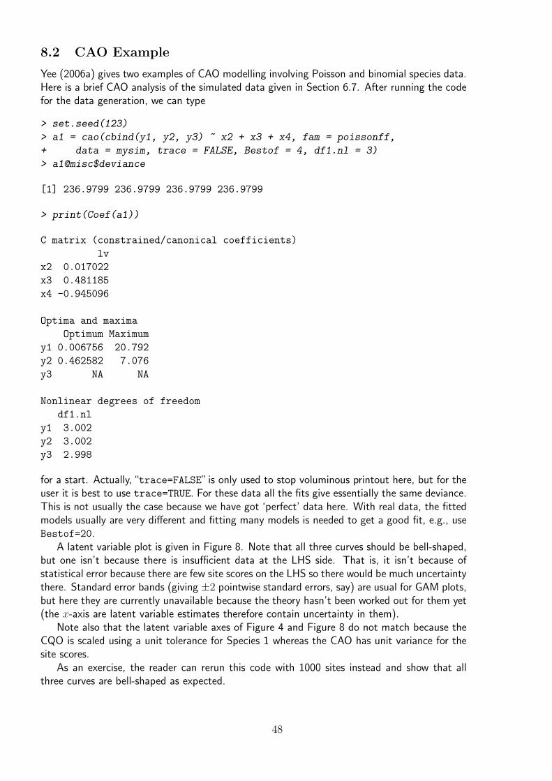
8.2 CAO Example
Yee (2006a) gives two examples of CAO modelling involving Poisson and binomial species data.Here is a brief CAO analysis of the simulated data given in Section 6.7. After running the codefor the data generation, we can type
> set.seed(123)
> a1 = cao(cbind(y1, y2, y3) ~ x2 + x3 + x4, fam = poissonff,
+ data = mysim, trace = FALSE, Bestof = 4, df1.nl = 3)
> a1@misc$deviance
[1] 236.9799 236.9799 236.9799 236.9799
> print(Coef(a1))
C matrix (constrained/canonical coefficients)
lv
x2 0.017022
x3 0.481185
x4 -0.945096
Optima and maxima
Optimum Maximum
y1 0.006756 20.792
y2 0.462582 7.076
y3 NA NA
Nonlinear degrees of freedom
df1.nl
y1 3.002
y2 3.002
y3 2.998
for a start. Actually,“trace=FALSE” is only used to stop voluminous printout here, but for theuser it is best to use trace=TRUE. For these data all the fits give essentially the same deviance.This is not usually the case because we have got ‘perfect’ data here. With real data, the fittedmodels usually are very different and fitting many models is needed to get a good fit, e.g., useBestof=20.
A latent variable plot is given in Figure 8. Note that all three curves should be bell-shaped,but one isn’t because there is insufficient data at the LHS side. That is, it isn’t because ofstatistical error because there are few site scores on the LHS so there would be much uncertaintythere. Standard error bands (giving ±2 pointwise standard errors, say) are usual for GAM plots,but here they are currently unavailable because the theory hasn’t been worked out for them yet(the x-axis are latent variable estimates therefore contain uncertainty in them).
Note also that the latent variable axes of Figure 4 and Figure 8 do not match because theCQO is scaled using a unit tolerance for Species 1 whereas the CAO has unit variance for thesite scores.
As an exercise, the reader can rerun this code with 1000 sites instead and show that allthree curves are bell-shaped as expected.
48

> lvplot(a1, lcol = 1:3)
−2 −1 0 1 2
0
5
10
15
20
Latent Variable
Fitt
ed v
alue
s
Figure 8: Latent variable plot of a1. This should be similar to Figure 4.
9 Ordinal Ordination
Ordinal responses obtained from an underlying Poisson or negative binomial distribution are acommon form of data. For example, in the biological sciences, it is common to measure speciesdata as an ordinal response taking levels 1, 2, . . . , L, say, where L ≥ 2. For example, 1 meansabsence, 2 means low abundance, 3 means medium abundance and 4 means high abundance.A specific example of this is the Braun-Blanquet scale in plant ecology with L = 7 levels. Theneed to measure the response as an ordinal factor often arises because it is too difficult tocount individuals, e.g., ants, diatoms, plankton are very small and/or moving. Instead, it ismore convenient to categorize the abundance into a factor Y ∗, say, with L levels. We haveY ∗ = l if Kl−1 < Y ≤ Kl for integer cut points or thresholds Kl (l = 1, 2, . . . , L) whereK0 = −∞ and KL = ∞. Here, Y ∗ the categorical response.
Yee (2006b) has developed a new methodology which allows ordination with ordinal speciesresponse. The main ideas are as follows. We assume the underlying count distribution (for arandom variable Y ) is either Poisson or negative binomial with
log µ = η (21)
where µ = E(Y ) and η is a linear or additive predictor in covariates x (Hastie and Tibshirani,1990). This is the natural and ideal situation. However, we are stuck with Y ∗ instead of Y .
With ordinal responses Y ∗, a very popular approach is to model the cumulative probabilitiesγl = pr[Y ∗ ≤ l]. For example, the proportional odds model has
g∗(pr[Y ∗ > l]) = η∗l , l = 1, 2, . . . , L− 1, (22)
where g∗ is the logit link and η∗l is a linear or additive predictor in x (see Yee and Wild (1996)).
49

Yee (2006b) has shown how it is possible to fit (21) by actually fitting (22). The key isto use new link functions, called the“Poisson-ordinal” link function (or POLF) or the“negativebinomial ordinal” link function (or NBOLF). The disadvantage with these is that the cut pointsmust be known, something which is not possible for all studies. However, we can approximatethe negative binomial distribution by a 2-parameter gamma distribution (giving a GOLF) and itis possible to obtain an approximate solution with the GOLF without knowing the cut points.
Note that, with Poisson counts and K1 = 0, it is recommended that a complementarylog-log link be used. That is, with presence/absence data coming from an underlying Poissondistribution, a constrained ordination should use the complementary log-log link instead of thelogit link which is more popular and is the default for cumulative().
Useful functions in the vgam package for ordinal ordination are listed in Table 8.
Table 8: A summary of vgam functions associated with ordinal ordination.
Function Purposegolf() gamma-ordinal link function, or GOLF.polf() Poisson-ordinal link function, or POLF.nbolf() negative binomial-ordinal link function, or NBOLF.nbolf2() Alternative NBOLF (based on a Camp-Paulson approximation).cumulative() vgam family function for ordinal regression.Cut() Converts counts to an ordinal responseoptim() General-purpose optimization function.
Here are some notes about the current vgam implementation of ordinal ordination.
1. The code is not finished! It is planned that invocations such as
cqo(ymat ~ x2 + x3 + x4 + x5,
fam=cumulative(link="polf", reverse=TRUE, mv=TRUE), data=d)
be done in FORTRAN—this is simple and clean for the typical user. Currently one needs todo it all in R, e.g., in the example below there is the need for a function (called newfun())to set things up and this is messy and complicated for the typical user. Hopefully theneed for such a function will be banished soon with the FORTRAN implementation.
2. The input/response to cumulative(mv=TRUE) is a matrix of ordinal responses takinginteger values 1, 2, . . . , L for each column. That is, each response must have some ofeach of L levels of the factor. This hopefully will be relaxed in the future. The outputfrom Cut() is specifically designed to be input for cumulative(mv=TRUE).
3. The link functions in Table 8 should be operated on the reverse cumulative probabilites,i.e., γc
l = 1 − γl to maintain a suitable direction for η∗l . This is so that the tolerancematrices are positive-definite for bell-shaped curves/surfaces. That is why reverse=TRUEis recommended.
4. When using nbolf() and polf() the cut points are entered using the earg argument.The component name of this list is "cutpoint". Since the reverse cumulative probabilitesare used, the "cutpoint" vector should be an increasing sequence. For example,
> prob = seq(0.1, 0.9, by = 0.2)
> polf(cbind(prob, prob), earg = list(cutpoint = c(5, 20)))
50

prob prob
[1,] 1.156667 2.736333
[2,] 1.541734 2.920352
[3,] 1.770706 3.038552
[4,] 1.976136 3.150155
[5,] 2.239844 3.301042
Here, the first argument of polf() must have two columns because there are twocut points. The function nbolf() requires k and the component name is simply "k".
5. When using golf() the cut points are optional. However, λ isn’t, and it is entered usingthe earg argument with component name "lambda".
6. For Cut() the argument breaks matches that of the S function cut(). It is recom-mended that the first and last values of breaks should be -Inf and Inf respectively.
9.1 Example
Here’s an ordinal ordination example from the hunting spiders data set. The following code isspecific to the hspider data frame, however you could adapt it for your own data set. We fita rank-1 equal tolerances CQO negative binomial model with k = 1 for each species.
> data(hspider)
> hspider[, 1:6] = scale(hspider[, 1:6])
> newfun = function(bic, mylink = "nbolf", lambda = 1, kay = 1,
+ dev = TRUE, omitcutpt = FALSE, trace = FALSE, mybreaks = c(-Inf,
+ 5, 20, Inf), altbreaks = c(-Inf, 1, 10, Inf), altspp = NULL,
+ spp. = c(7, 8, 9, 10, 11, 12, 14, 15, 16, 17, 18))
+ xmat = as.matrix(hspider[, 1:6])
+ lv1 = c(xmat %*% cbind(bic))
+ lv12 = -0.5 * lv1 * lv1
+ matMYbreaks = matrix(mybreaks, length(mybreaks), 18)
+ if (is.Numeric(altspp))
+ matMYbreaks[, altspp] = altbreaks
+ LLength = nrow(matMYbreaks) - 1
+ allmyb = c(matMYbreaks[2:LLength, spp.])
+ ycut = Cut(hspider[, spp.], breaks = mybreaks)
+ counter = 1
+ for (ii in spp.)
+ ycut[, counter] = Cut(hspider[, ii], breaks = matMYbreaks[,
+ ii])
+ counter = counter + 1
+
+ if (mylink == "polf")
+ earg = list(cutpoint = allmyb)
+ if (mylink == "nbolf")
+ earg = list(cutpoint = allmyb, k = kay)
+ if (mylink == "golf")
+ if (omitcutpt)
+ earg = list(lambda = lambda)
51

+
+ else
+ earg = list(cutpoint = allmyb, lambda = lambda)
+
+
+ M = LLength - 1
+ NOS = length(spp.)
+ mylist = list("(Intercept)" = if (mylink == "golf")
+ if (length(earg$cutpoint)) kronecker(diag(NOS),
+ matrix(1, M, 1)) else kronecker(diag(NOS),
+ diag(M))
+ else kronecker(diag(NOS), matrix(1, M, 1)), lv1 = kronecker(diag(NOS),
+ matrix(1, M, 1)), lv12 = kronecker(matrix(1, NOS,
+ 1), matrix(1, M, 1)))
+ fit = vglm(ycut ~ lv1 + lv12, constraint = mylist,
+ cumulative(link = mylink, rev = TRUE, mv = TRUE,
+ par = TRUE, earg = earg, intercept.apply = TRUE),
+ trace = trace)
+ if (dev)
+ deviance(fit)
+ else fit
+
The function newfun() above uses two sets of cutpoints over all species. For example, rarespecies can be handled by the argument altbreaks having lower values for the cut points. Thefunction newfun() fits the CQO given the values of c in the argument bic. The list mylistcontains the constraint matrices; understanding the technical details requires knowledge aboutVGLMs and QRR-VGLMs in general.
Now we will get initial values for the constrained coefficients c by fitting an ordinary CQOto the counts.
> ymat = as.matrix(hspider[, -(1:6)])
> p1 = cqo(ymat ~ WaterCon + BareSand + FallTwig + CoveMoss +
+ CoveHerb + ReflLux, fam = poissonff, trace = FALSE,
+ data = hspider, Crow1positive = FALSE, ITol = TRUE,
+ Bestof = 4)
> sort(p1@misc$deviance.Bestof)
[1] 1585.133 1719.542 2472.063 2472.070
> if (deviance(p1) > 1586) stop("suboptimal fit obtained")
> round(c(ccoef(p1)), dig = 2)
[1] -0.36 0.55 -0.92 0.32 -0.31 0.70
Now we can finally solve for c with ordinal ordination! The following code requires asubstantial amount of number crunching and can take a minute or two to run.
> set.seed(123)
> solveit = optim(par = c(ccoef(p1)), method = "L-BFGS-B",
+ fn = newfun, altspp = c(9, 10, 11), altbreaks = c(-Inf,
52

+ 0, 10, Inf), mylink = "nbolf", kay = 1, trace = FALSE,
+ lower = -Inf, upper = +Inf)
> solveit$value
[1] 232.1201
> solveit$par
[1] -0.1692321 0.7802340 -0.6223791 0.5538531 -0.1043394 0.9682084
> if (solveit$convergence != 0) stop("did not converge")
Now we scale the solution so that the species have unit tolerances.
> fit <- newfun(solveit$par, dev = FALSE, altspp = c(9, 10,
+ 11), altbreaks = c(-Inf, 0, 10, Inf), mylink = "nbolf",
+ kay = 1, trace = FALSE)
> ssoln = solveit$par * sqrt(coef(fit)[length(coef(fit))])
> fit <- newfun(ssoln, dev = FALSE, altspp = c(9, 10, 11),
+ altbreaks = c(-Inf, 0, 10, Inf), mylink = "nbolf",
+ kay = 1, trace = FALSE)
> deviance(fit)
[1] 232.1201
> coef(fit)["lv12"]
lv12
1
> round(ssoln, dig = 2)
[1] -0.19 0.89 -0.71 0.63 -0.12 1.11
(We checked the unit tolerances by seeing that the coefficient for the "lv12" is 1). Here, ssolnis the scaled solution. Looking at the results, we can see that the constrained coefficients fromthis ordinal ordination have the same sign as that of the raw count data. This is reassuring; itshows there is some stability in the ordination. Fitting various ordinal CQO and CAO models(and with Poisson, negative binomial and gamma links) shows that the signs of the constrainedcoefficients do not seem to change much—see the Exercises.
It is expected that ordinal ordination should work reasonably well, especially for large sim-ulated data sets. Given the current software limitation that each species must have the samenumber of levels, how many levels should be used? From a practical point of view, I currentlyrecommend L = 3 or 4. Decreasing L means there is less sensitivity to outliers in the response.Increasing L means less information loss, but with L too large it becomes more difficult to findcut points that work well in data sets with both rare and abundant species.
Just to finish the example, note that
> fit@y
53

1 2 3 1 2 3 1 2 3 1 2 3 1 2 3 1 2 3 1 2 3 1 2 3 1 2 3 1 2 3 1 2 3
1 0 0 1 0 1 0 1 0 0 1 0 0 1 0 0 1 0 0 0 0 1 0 1 0 0 0 1 0 0 1 1 0 0
2 1 0 0 1 0 0 1 0 0 1 0 0 1 0 0 0 0 1 1 0 0 0 1 0 0 0 1 0 0 1 0 1 0
3 0 1 0 0 1 0 0 1 0 0 1 0 1 0 0 0 1 0 0 0 1 0 1 0 0 0 1 0 0 1 1 0 0
4 1 0 0 0 1 0 1 0 0 0 1 0 1 0 0 0 0 1 0 1 0 0 0 1 0 0 1 0 0 1 0 0 1
5 1 0 0 0 1 0 1 0 0 0 1 0 1 0 0 0 1 0 1 0 0 0 0 1 0 0 1 0 0 1 0 1 0
6 1 0 0 0 1 0 1 0 0 0 1 0 1 0 0 0 1 0 0 1 0 0 0 1 0 0 1 0 0 1 0 0 1
7 1 0 0 0 1 0 1 0 0 0 0 1 1 0 0 0 1 0 0 0 1 0 0 1 0 0 1 0 0 1 0 1 0
8 1 0 0 0 1 0 1 0 0 1 0 0 1 0 0 0 1 0 1 0 0 1 0 0 1 0 0 0 0 1 1 0 0
9 1 0 0 1 0 0 1 0 0 1 0 0 1 0 0 1 0 0 0 0 1 1 0 0 1 0 0 1 0 0 1 0 0
10 1 0 0 1 0 0 0 1 0 1 0 0 1 0 0 1 0 0 0 0 1 1 0 0 1 0 0 1 0 0 1 0 0
11 0 1 0 1 0 0 0 1 0 1 0 0 1 0 0 1 0 0 0 0 1 1 0 0 1 0 0 1 0 0 1 0 0
12 0 1 0 0 1 0 1 0 0 1 0 0 1 0 0 1 0 0 0 0 1 1 0 0 0 1 0 0 1 0 1 0 0
13 1 0 0 0 0 1 0 1 0 0 1 0 1 0 0 0 1 0 0 0 1 0 0 1 0 0 1 0 0 1 0 0 1
14 1 0 0 1 0 0 1 0 0 0 1 0 1 0 0 1 0 0 0 1 0 0 1 0 0 0 1 0 0 1 0 0 1
15 1 0 0 1 0 0 1 0 0 1 0 0 1 0 0 1 0 0 1 0 0 1 0 0 1 0 0 0 0 1 1 0 0
16 1 0 0 1 0 0 1 0 0 1 0 0 1 0 0 1 0 0 1 0 0 1 0 0 1 0 0 0 0 1 1 0 0
17 1 0 0 1 0 0 1 0 0 1 0 0 1 0 0 1 0 0 1 0 0 1 0 0 1 0 0 0 0 1 1 0 0
18 1 0 0 1 0 0 1 0 0 1 0 0 1 0 0 1 0 0 1 0 0 1 0 0 1 0 0 0 0 1 1 0 0
19 1 0 0 1 0 0 1 0 0 1 0 0 1 0 0 1 0 0 1 0 0 1 0 0 1 0 0 0 0 1 1 0 0
20 1 0 0 1 0 0 1 0 0 1 0 0 1 0 0 1 0 0 1 0 0 1 0 0 1 0 0 0 0 1 1 0 0
21 1 0 0 1 0 0 1 0 0 1 0 0 1 0 0 1 0 0 1 0 0 1 0 0 1 0 0 0 1 0 1 0 0
22 0 1 0 1 0 0 0 0 1 1 0 0 0 1 0 1 0 0 1 0 0 1 0 0 1 0 0 1 0 0 1 0 0
23 0 1 0 1 0 0 0 0 1 1 0 0 0 1 0 1 0 0 0 1 0 1 0 0 1 0 0 1 0 0 1 0 0
24 0 1 0 1 0 0 0 0 1 1 0 0 0 1 0 1 0 0 1 0 0 1 0 0 1 0 0 1 0 0 1 0 0
25 0 1 0 1 0 0 0 1 0 1 0 0 1 0 0 1 0 0 0 1 0 0 1 0 1 0 0 0 1 0 0 1 0
26 1 0 0 1 0 0 0 1 0 1 0 0 0 0 1 1 0 0 1 0 0 1 0 0 1 0 0 1 0 0 1 0 0
27 0 0 1 1 0 0 0 0 1 1 0 0 0 1 0 1 0 0 1 0 0 1 0 0 1 0 0 1 0 0 1 0 0
28 0 1 0 1 0 0 0 0 1 1 0 0 0 1 0 1 0 0 0 1 0 1 0 0 1 0 0 1 0 0 1 0 0
Here, the first three columns correspond to the first species, etc. and the column names are lfor l = 1, . . . , L. A 1 indicates the presence of that level, otherwise a 0, so fit@y is a matrixof indicator variables really. Each column must contain at least one 1 and one 0.
54

10 Not Yet Been Implemented
The following is a list of things not yet been implemented in vgam.
1. Along the lines of Fu (2003) and Fu (1998), one could apply a Lasso type operator tothe latent variables. This would mean that some of the coeffients would be zero, andpossibly the log-likelihood function would be unimodal rather than multimodal. Thisneeds investigation.
Software Changes
[12 Jan 2004] biplot.qrrvglm() merged with lvplot.qrrvglm(); the two functionsare equivalent.
[27 Sep 2005] FastAlgorithm=FALSE is not allowed.
[17 Oct 2005] An undocumented faster algorithm is implemented when ITolerances=TRUE.
[7 Aug 2006] ITolerances=TRUE is now the default.
Exercises
1. More general than (6) is
η = BT1 x1 +
K∑k=1
AkCTk xk+1,
where K is any specified positive integer, Ak is M × Rk and unknown, and xk is apk-vector with p1 + · · · + pK+1 = p. This is currently not yet implemented in vgam.Discuss the computational details behind estimating such a model.
2. In the example of Section 5.2, corner constraints were used. Repeat the analysis withsummation constraints,
∑i αi =
∑j γj = 0, and reconcile the estimated regression coef-
ficients.
3. Search the literature for a model that has many parameters for which a reduced-rank fitwould be a good idea. Write a vgam family function for the model and run it underrrvglm() on a suitable data set. Does a biplot add to your understanding?
4. Suppose Wi, i = 1, . . . , n, are general M × M positive-definite matrices and Z is ageneral n × M matrix. Suppose we wish to approximate Z by a specified lower rankmatrix Z = ACT where A is n×R and C is M ×R. One can do this by minimizing
‖Ω ∗(Z− Z
)‖2 =
n∑j=1
M∑k=1
(Ω)jk
(zjk − aT
j ck
)2, (23)
where Ω is an associated weight matrix and ∗ is the Hadamard (element-by-element)product. Show that this may be solved by an alternating algorithm. Hint: look at theunderlying minimization problem behind vgam. [Gabriel and Zamir (1979)]
55

5. In the car example, show that a MLM treating A as known and fixed produces standarderrors that are smaller than that obtained from the RR-MLM. Of course, your fittedcoefficients should be identical of the RR-MLM.
6. Suppose one runs
rrvglm(ymatrix ~ bs(x, 4), family=multinomial, Rank=1, Corner=TRUE)
Show that this is a multinomial logit model with
ηj = β(j)0 + ajf(x), a1 = 1, j = 1, . . . ,M,
where f is a smooth function of x estimated by a B-spline. If“multinomial”is replacedby“cumulative”the curves won’t intersect if aj are all the same sign and f is monotonic.
7. Consider a rank-1 Poisson CQO model with x1 = 1. Let tj be the tolerance of species j.Show that
µj(uj ± k tj)
µj(uj)= exp
−1
2k2
(24)
where k > 0. This says that if you are k tolerance units away from the species’ optimumthen the ratio of the mean abundance there relative to the species’ maximum declinesexponentially in −1
2k2. Show that the RHS of (24) is also the corresponding expression
for the rank-2 equal-tolerances Poisson CQO model with Tj = I2 when k is the Euclideandistance away from the species’ optimum. Is this true for general rank-R?
8. Consider the CQO model when ITolerances=TRUE. Discuss the uniqueness of the pa-rameters for this model.
9. Extend the example of Section 6.7 by generating data from a rank-2 model, and thenfit a rank-2 QRR-VGLM. Obtain a latent variable plot, and check that it gives sensibleoutput. Also check that the output from summary() and Coef() is ‘right’.
10. In the example of Section 9.1, k = 1 was used for all species. Suppose all species have acommon k value but k 6= 1. Perform the ordinal ordination for various values of k andso maximize a profile likelihood. What is the optimal k to one decimal place accuracy?
11. Using newfun() for a start, fit various ordinal ordinations to the hunting spiders data.Vary the link function and the cut points. Do the results appear to change much?
References
Ahn, S., Reinsel, G. C., 1988. Nested reduced-rank autoregressive models for multiple timeseries. Journal of the American Statistical Association 83, 849–856.
Anderson, J. A., 1984. Regression and ordered categorical variables (with discussion). Journalof the Royal Statistical Society, Series B, Methodological 46, 1–30.
Anderson, T. W., 1951. Estimating linear restrictions on regression coefficients for multivariatenormal distributions. The Annals of Mathematical Statistics 22, 327–351.
56

Chambers, J. M., Hastie, T. J. (Eds.), 1993. Statistical Models in S. Chapman & Hall, NewYork.
Fiocco, M., Putter, H., van Houwelingen, J. C., 2005. Reduced rank proportional hazards modelfor competing risks. Biostatistics 6, 465–478.
Fu, W. J., 1998. Penalized regressions: The bridge versus the lasso. Journal of Computationaland Graphical Statistics 7, 397–416.
Fu, W. J., 2003. Penalized estimating equations. Biometrics 59, 126–132.
Gabriel, K. R., Zamir, S., 1979. Lower rank approximation of matrices by least squares withany choice of weights (corr: V22 p136). Technometrics 21, 489–498.
Goodman, L. A., 1981. Association models and canonical correlation in the analysis of cross-classifications having ordered categories. Journal of the American Statistical Association 76,320–334.
Greenland, S., 1994. Alternative models for ordinal logistic regression. Statistics in Medicine13, 1665–1677.
Hastie, T. J., Tibshirani, R. J., 1990. Generalized Additive Models. Chapman & Hall, London.
Hastie, T. J., Tibshirani, R. J., Friedman, J. H., 2001. Elements of Statistical Learning: DataMining, Inference and Prediction. Springer-Verlag, New York.
Heinen, A., Rengifo, E., 2005. Multivariate reduced rank regression in non-Gaussian contexts,using copulas. Preprint submitted to Journal of Multivariate Analysis, 9 July 2004 .
McCullagh, P., 1980. Regression models for ordinal data. Journal of the Royal Statistical Society,Series B, Methodological 42, 109–142.
McCullagh, P., Nelder, J. A., 1989. Generalized Linear Models, 2nd Edition. Chapman & Hall,London.
Oksanen, J., Minchin, P. R., 2002. Continuum theory revisited: what shape are species responsesalong ecological gradients? Ecological Modelling 157, 119–129.
Reinsel, G. C., Velu, R. P., 1998. Multivariate Reduced-Rank Regression: Theory and Applica-tions. Springer-Verlag, New York.
Ruppert, D., Wand, M. P., Carroll, R. J., 2003. Semiparametric Regression. Cambridge Univer-sity Press, Cambridge.
van Eeuwijk, F. A., 1995. Multiplicative interaction in generalized linear models. Biometrics 51,1017–1032.
Venables, W. N., Ripley, B. D., 2002. Modern Applied Statistics With S, 4th Edition. Springer-Verlag, New York.
Wartenberg, D., Ferson, S., Rohlf, F. J., 1987. Putting things in order: a critique of detrendedcorrespondence analysis. The American Naturalist 129, 434–448.
Yee, T. W., 2004. A new technique for maximum-likelihood canonical Gaussian ordination.Ecological Monographs 74, 685–701.
57

Yee, T. W., 2005. On constrained and unconstrained quadratic and additive ordination.Manuscript in preparation .
Yee, T. W., 2006a. Constrained additive ordination. Ecology 87, 203–213.
Yee, T. W., 2006b. Ordinal ordination with normalizing link functions for count data. Submittedfor publication .
Yee, T. W., Hastie, T. J., 2003. Reduced-rank vector generalized linear models. StatisticalModelling 3, 15–41.
Yee, T. W., Mitchell, N. D., 1991. Generalized additive models in plant ecology. Journal ofVegetation Science 2, 587–602.
Yee, T. W., Wild, C. J., 1996. Vector generalized additive models. Journal of the Royal Statis-tical Society, Series B, Methodological 58, 481–493.
58