RANK CORRELATION AND REGRESSION IN ......RANK CORRELATION AND REGRESSION 179 difficult to choose...

RANK CORRELATION ANDREGRESSION IN A NONNORMAL

SURFACEF. N. DAVID' AND EVELYN FIX2UNIVERSITY OF CALIFORNIA, BERKELEY

1. The problem

The problem, seemingly simple, which led to the work reported in this paper,was this: to find a "usable" test for a difference in position of two regressionlines if it is known that the two lines have the same slope but it is also knownthat the marginal distributions are extremely skewed and one is loath to usetransformations and normal theory may be inadequate. More precisely, we con-sider the following situation. Suppose that there are two sets of bivariate cor-related observations, ni in the first set and n2 in the second set, with ni + n2 = n.Neither the functional form of the bivariate population (or populations) nor ainyof the parameters descriptive of the population (populations) from which theobservations have been drawn is known. However, the number of observations(between 20 and 50) is sufficient to indicate that the marginal distributions maybe extremely skew Type III and the regression may be linear. Furthermore, fromthe description of the experiments generating the bivariate observations, it seemsreasonable to assume that, if indeed they do come from different populations,the regression lines of the parent populations have the same slope with the dif-ference occurring in the intercepts or position of the lines. The data may beanalyzed in a variety of ways, including the orthodox one of transforming thedata and using normal theory tests. Here we discuss the possibility of usingtests based on the rank correlation coefficient attributed to Spearman. We pro-pose the use of these tests in their conditional form. In order that the criteriaproposed may be compared with others, we suggest a bivariate functional formfor the population, which we have been unable to find discussed elsewhere andwhich enables us to throw some light on the behavior of the mean value ofSpearman's rho when the population is nonnormal.

2. Rank correlation in the normal correlation distribution

Before proceeding with the discussion of the problem outlined, it is useful torecall what is known about Spearman's rho in the case of the bivariate normal

1 This paper was prepared with the partial support of the Office of Naval Research (Nonr-222-43).

2 This investigation was supported (in part) by a research grant (No. RG-3666) from theNational Institutes of Health, Public Health Service.

177

178 FOURTH BERKELEY SYMPOSIUM: DAVID AND FIX

distribution when the correlation is not zero. Suppose that n pairs of observa-tions {xi, yiJ are randomly and independently drawn from a bivariate normalpopulation with correlation p. The {xi} and {yi} are each ranked in order ofmagnitude. The product moment correlation between the ranks, r8, is, of course,Spearman's p. Sundrum [6] derived the exact distribution of r8 for n = 3. Ingeneral for all n, it is known (Moran [3]) that

(1) E(r8,) = ( 6 1) [sin-' p + (n -2) sin-12P].Kendall [2], modified by Fieller, Hartley, and Pearson [1], gave

(2) ar2 - 1 [1 -1.56.h345p2 + 0.304743p4 + 0.155286p6+ 0.061552p8 + 0.022099p" + 0.019785p12].

David, Fix, anid Mallows, in ani unpublished manulscript, have shown that, toorder p2, this variance is

(3)2 1 3p2

n - 1- 7r2n (2)(n + 1)2 [(19n' - 89n2 + 168n - 108) - 8\3(n-1n-

Fieller, Hartley, and Pearson suggested from an empirical investigation that, if

(4) Z =Ilog1 + r,

then z is approximately normally distributed. If we write E(r8) = R, then1 +R + 2 R

(5) E(z) 9log I R (I R 2)2

and

(6) Varz .' , 1( 2)2

This may be applied in the two sample problem to deriving a test for the equiva-lence of the slopes of the two regression lines. Thus, if ri and r2 are the rankcorrelation coefficients of each sample ranked separately and the correspondingtransforms z1 and Z2 are calculated, the criterion under the null hypothesis of nodifference of slope,

(Zl - Z2)(1 - R2)(7)~~~~~~~~~a2, + 0.2) /(0o7 -I 2112

is approximately a unit normal variable.

3. Criteria for position

The equivalence of position of two regression lines in terms of ranks does notappear to have been discussed. If one desires to analyze data in this way, it is

RANK CORRELATION AND REGRESSION 179

difficult to choose criteria except by very general considerations, for there is noreally workable procedure such as the likelihood ratio which will indicate theappropriate test to use against specified alternatives. Four criteria are put for-ward here, the first two by analogy with orthodox normal theory for the originalobservations, the last two on common-sense grounds. We consider the problemin the following terms.Under the null hypothesis Ho, there will be one population 11. Let

(8) E(x) = t, E(y) =i.Under the alternative hypothesis Hi, there will be two populations HIl and 112. Let

(9) E(xlHIl) = ti, E(yjIh) = 71,

E(xfll2) = t2, E(yIll2) = X72-It should be recognized that, although the problem seems very like that oftesting the difference between two means, there is a difference in that one hasthe additional information that the slopes of the regression lines under HI arethe same and this information should not be ignored.

In terms of ranks, write R., for the rank of xi and Rj, for the rank of yi. Forall four criteria designed to test a variant of Ho and sensitive to a variant ofHi, it is assumed that the two samples are ranked together but that calcula-tions are carried out on these ranks relating to one sample only.

(i) HO: tl = t2 = t. Hl:tl 0 t2-Recall for a moment the situation in which there is a bivariate normal dis-tribution with marginal means t and'7, marginal standard deviations unity andcorrelation coefficient p, assumed known. Given a bivariate normal samplexi, yi, i = 1, 2, * * , n, from this distribution, we wish to test the hypothesisthat t = to (some specified value) against the alternative that t #, to. The likeli-hood ratio criterion is(10) -py.When p is not known, the criterion(11) -rymight be used where r is the sample product moment correlation coefficient.

Let R., and Ry, be the ranks of the pair xi, yi belonging to the first set ofobservations, ni in number, the ranks, however, as given by the combinedranked sample. By analogy with the procedure for the bivariate normal sur-face, we choose the criterion

(12) na=- [Rxi- n -r, (RyC _ n +l

where the sum is over only those observations which belong to the first set of n,observations indicated by n1. Further, r, is the Spearman product moment cor-relation coefficient for the combined set of n observations and a2 = (n2 - 1)/12.


A similar criterion to test

Ho: 1 = '72 ='7, Hi: 77,$ 72,will be

(13) Tn1 = Ry - n_ + __(R._n+ )

(ii) Ho: t1= 2 = t 71 =772 = 77-

HI: j # t2, 7 1 272-

Again, one recalls that, given the same normal distribution as in (i) with pknown, the likelihood ratio test procedure yields the criterion,

(14) (x-_ t)2 -2p( - t)(y - n) + (y - X17)2.This suggests that the appropriate rank criterion would be

(15) T2 = 2 2{[ (RZi- 2 )]

r,[ n (Rn

2 1)][F_ (Ryi _n

)] + [T_ (Ryi _ n + I1)]2}-It is certain that the criteria T1 and T2 are not the optimum possible since

the original variables {xi, yi} are not normally distributed whereas the criteriaare based on analogy with criteria obtained from underlying normality. Twoother criteria may be suggested on common-sense grounds. These are theaverage of the sum of the distances from the line R. = Ry for one set of observa-tions as one possibility and the average of the sum of the distances from theline Ry = -Rz + (n + 1) as the other. Thus,

(iii) Ho: t1= t2 = t, 171 = 772 = 7;

HI: tl > t2, 771 < 772; t1 < t2, 711 > 712-

The criterion is

(16) sP = a (Rxi -Rj)Similarly, given that

(iv) Ho: t1 = t2 771 = 12 = 71;

Hl: tl < t2, 771 < 772; tl > t2, 11 > t12pthe criterion is

(17) 0=1 E [Rxi + Ryi- (n + 1)]

4. Conditional tests

Consider any one particular combined ranked sample and, for the sake of anexample, the criterion T1. There will be n pairs of ranks and we may constructn quantities


(18) d= (Ri _ n + I)-r (Ry _ n +1)

This set of {dj} can be looked on as a finite population of n with polykays,1 n

K1 = n E dj = 0,(19) 12j-)

-n Kil = K2=aj1,d> (1rs)n-p1i ' n -i

The second and higher polykays of this set are conditional on the r, that is, onthe particular combined sample, as is expected. We treat the {d,} as a randomiza-

tion set and consider all possible (n ) samples of ni which may be generated from

it. T1 is the mean of a sample of ni which under the null hypothesis is randomlydrawn without replacement from the finite population of the {d,}. Accordingly,from known results,

oyE(Ti) = 0,(20) 11 1\ a2(n - n1)

'2Var (Ti) = K2I(---) = n( -1) (1-r2)or

(21) VarT[12) 1/2 = n n

L(1 ~r.)I n1(n - 1

The third and fourth polykays are

(22)

K3 = (3) £ dj, K4 = n){(n + 1)E2 di - 3(n -1

whence

(23) )2 I3(Ti)= iL(k! )(;l - d)

and

(24) a24(T1) = K4 [(- ) 1- 1)2 + n -

3(n-1)(1 1\)2 2 4).~ I-- (Kn+1 \n, nlnWhen n1 = n2 the third moment is zero and, in general, provided ni is not verydifferent from n2 the distribution of T1 will not be far off normal. The distribu-tion exhibits the expected saw-tooth effect characteristic of rank distributionsand the 02 is usually less than three. The significance levels for T1 given j1 and 32may be found directly from table 42 (Pearson and Merrington) in [5]. Usually,however, it will be enough to assume normality. The conditional test which we


(a)

-12 -10 -8 -6 -4 -2 0 2 4 6 8 10 12

(b)

-16 -14 -12 -10 -8 -6 -4 -2 0 2 4 6 8 10 12 14 16

(C)

-14 -12 -10 -8 -6 - 4 -2 0 2 4 6 8 10 12 14

FIGURE 1

Rtandomizationi distribution of niaop for a sampleof n, = 5, for three particular samples of 10.

Sample before ranking is bivariate normal, p = 0.5

and (10) = 252. Finite population.5

Samnple (a): d = -3, -1, 0, 0, 0, 8, 4, -2, -4, -2; 02 = 2.15.

Sample (b): d = 2, -2, 4, -4, 6, 0, -5, -5, 4, 0; 02 = 2.66.

Sample (c): d = 3, 7, -5, -5, -1, -1, 2, 1, -3, 2; 02 = 2.48.


propose is that T'1/(l - r,)1/2 be considered as a normal variable with variancen2/ni(n - 1). The effect of 2 < 3 will be to make the first kind of error lessthan that nominally given by the assumption of normality.The same procedure may be used for so and 0. We have that

E((p) = 0 = E(@),(25) 2 (n ) = 0Var 1 Var[IL( r8)1/2 ni(n -1 [( +r.) 12jThen S/(1- r8)1/2 and 0/(1 + r,)"/2 may each be assumed to be normally dis-tributed. For purposes of illustration, the randomization distributions for n1a¢o,n = 10, n1 = 5 are given in figure 1 for three samples drawn from a bivariatenormal with p = 0.5. It will be noted that even with such small numbers theassumption of normality for the distribution is not unseemly. Numerical com-parisons of the critical levels are given in table I.

TABLE I

COMPARISONS OF THE CRITICAL VALUES

Sample (a) (b) (c)

Critical level 210 211 212 |12 214 ,16 211 212 213 215

True .040 .016 .004 .036 .016 .008 .040 .028 .012 .004Normal .046 .031 .021 .034 .016 .007 .039 .027 .018 .008Pearson-Merrington .042 .020 .006 .032 .014 .... .039 .024 .013 ....

The criterion T2 is the mean of a sum of squares. In the randomization setit may be assumed that T2 is distributed (approximately) proportionally as x2

with two degrees of freedom. We have that

(26) E(T2) = (n- 1) (1 -r2)

and the test of significance may be carried out from reference to the x2 tables.

The agreement between the distribution of the (n ) values of T2 and the modified

x distribution is not very close for small samples and its use is not recommendedfor samples less than 10 + 10 = 20.

If we write

(27) t2 n1(n - ) T2,n2(1 - r.)then t2 is distributed (approximately) directly as x2. Table II gives the meanand standard deviation of t2 in the randomization set when the original samplebefore ranking is randomly and independently drawn from the normal bivariatedistribution with correlation p = 0.5.

50-

40 - (a)

30

20L

10

0 1 2 3 4 5 6 7 8

t2

70

60

50 (b)

40-

30.

20-

10 .I0

0 1 2 3 4 5 6 7 8

50

40 - (c)

30 -

20-

10.0

0 1 2 3 4 5 6 7 8 9ta

FIGURE 2


TABLE II

CRITERION t2 (OR T2) WHEN THE ORIGINAL SAMPLEIs BIvARiATE NORMAL (p = 0.5)

Standardn n1 r. Mean t2 Deviation of t2

10 5 0.636 2 1.71610 5 0.091 2 1.72010 5 0.467 2 1.70310 4 0.636 2 1.7029 4 0.733 2 1.5667 3 0.679 2 1.5016 3 -0.257 2 1.481

Three of the randomization distributions of t2 are given in figure 2. As n, thecombined sample size, increases and if ni is not very different from n/2, it is tobe expected that the randomization distribution will be more closely approxi-mated by the X2 or the modified xA distribution.

5. Mean value of r, for any surface

For all four criteria, the variances given in the preceding section are dependenton r,, the rank product moment correlation coefficient of the particular sample.If it is required to use the criteria in an unconditional test, then it becomesnecessary to discuss E(r,) for T1, (p, and 6, and E(r!) for T2. Such a discussionwill need to be referred to the particular surface which it is thought mightdescribe the original unranked observations. We begin with a few general con-siderations.

Define a function H(t) such that

(28) {-~~~~~~~~1,t > O.Then

n ~~~~~~~~n(29) Rj - 1 = L2H(xi-xi), Ryi - 1= E H(y,- y.)

=1 ~~~~~m-1

FIGURE 2

Randomization distribution of t2.Finite population; n = 10 = 5 + 5.

Sample (a): Rj, = 8, 7, 3, 5, 4, 2, 6, 9, 1, 10;Ryi = 8, 4, 1, 3, 5, 6,10, 9, 2, 7.

Sample (b): Rzx = 4, 1, 3, 7, 8, 6, 2, 10, 9, 5;Ryi = 7, 3, 6, 10, 1, 8, 2, 5, 4, 9.

Sample (c): Rxi = 1, 8, 9, 4, 5, 2, 6, 7, 10, 3;Ry. = 5, 10, 7, 6, 2, 3, 9, 8, 4, 1.


and since

(30) r2 (2we have that

where 5~~~~~~~_(n 1)2(31) r= 2

wheren n n

(32) S = ,2 ; H(xi - xj)H(yi - yi).i=i j=1 mri

Consequently the expectation of r8 reduces to the expectation of S which will be

(33)E(S) = n(3)P{x, > yj, yi > y-li 'd j F4 m} + n(2)P{x, > x1, y, > yj i $ j}

= n(3)P + n(2)P2,

say, and

(34) E(r,) = 1 (n-2)Pj + P2-1

(n-1)

This is the technique which Moran applied for evaluating E(rT) for the bivariatenormal distribution and for which he found

(35) l 2 2r 2 P2 = 2-2 cos-r p.It is clear that the functional form assumed for the bivariate population distri-bution will affect the mean value of r8.

6. Double Gamma distributions

In the first section we stated that the set of bivariate observations was suchthat the margins might be described by extremely skew Type III distributionsand the regressions could be linear. This suggests that a surface with Type IIImargins might be a suitable functional form to describe the parent populationgenerating the samples. Rhodes [4] proposed a surface of this kind which alsohad linear regressions. He was followed by Van Uven [7], who did not seem tobe aware of Rhodes' work and who proposed essentially the same surface.Rhodes' distribution is however unsuitable for the present purposes since it isconstrained to lie within a wedge-shaped area whereas we require the bivariatesurface to take all values between zero and infinity. To meet the conditions ofthe problem we devised a distribution which must be known although it is newto us.

It was Weldon, in his well-known dice problem, who first suggested taking


three independent variables x, y, z and studying the surface formed by X, Y,where(36) X = x +y, Y = x +z.In Weldon's case, x, y, and z were each binomially distributed but it is clearthat his distribution is only one of a broad class of bivariate populations result-ing from the addition of independent random variables. This will be discussedelsewhere by C. L. Mallows. For present purposes, we propose the addition ofindependent Gamma variables. The resulting surface has the merit of simplicitybut has a discontinuity of functional form which is not entirely satisfactory.

Let A, B, and C be independent random variables with1A 1 1-

p(A) = j- Aa-le-A, p(B) = - BbleBr(a) F(b)(37) 1

p(C) = r(c) Cc-ie-c, a, b, c > 0; A, B, C >O.

Define(38) U = A +B, V = A +C,whence

eUV min U,V(39) p(UV) uP(a)(b) (c) Aa-l(U - A)b-l(V - A)e-leA dA.

In order to display the properties of the surface, we may also build it up in thefollowing way. The cumulants of A are Kr = a(r - 1)! and similarly for Band C. The center of the distribution is at (a + b, a + c), the correlation be-tween U and V is

a(40) =(40) P = ~~~~[(a+ b)(a + c)1/21and

(41) P(U) =~~Ua+b-Ie-U

(41) p(U) = r(a + b)

For the regression we consider the moments of V for U fixed and vice versa.We have

(42) p(AB) = Aa-lBb-le-(A+B)r(a)r(b)so that if we write

A _A(43) 9 U' G = A + B = U,

then, integrating out G,

(44) p (g) = p (A) ( =r(a + b) ga-l(l _ g)b-1.U r(a)r(b)


Accordingly for U fixed

(45) Kr(VIU) = Kr(C) + UTK,(g), E(V|U) = c + UKI(g).The cumulants of C are c(r - 1)! = K7 for r = 1, 2, * and the cumulants of gare those of a Type I variable of which the first four are

aKj(g) = A = a + b,

abK2(9) = A2(A + 1)'

(46)2ab(b - a)K3(g) = A3(A + 1)(A + 2)'

3ab (b - a)2 ab(A + 2)1r4(g) =A2(A + 1)(A + 2)(A + 3) L A2 A2(A + 1)J

The regression of V on U, that is,

(47) E(VI U) = C + U a+b

is linear no matter what a, b, and c and thus by symmetry so is the regressionof U on V. We thus have a distribution with Type III margins and linear regres-sions which extends over the whole plane 0 < V, U < +o0.

Since C and A are assumed independent,

(48) p(ACIU) = r(a +b)_) (A)-1 (1 _AU) -leCr'(a)r(b)r(c) \U/ U / U

or= r(a + b) (A\a1' A b-I eV

(49) p(AVIU) =l(a(b)r(c) (-U)(Vj- A)C- Uor

(50)

P(VIU) r(a + b)e-V minU,V

p(VjU) -r(a)r'(b)r(c)Ua+b-l J Aa-l(U - A)b-1(V - A)cleA dA,

while-(u+V rmin U,V

(51) p(UVC) eF Aal(U- A)l'(V - A)-leA dA.

In general, it does not seem possible to carry out an integration for A whichwill result in a distribution which will itself be integrable. The conditions of theoriginal problem, however, required the margins to be skew and this impliesthat a, b, and c should not be large in order to meet these required conditions.We have evaluated some special cases.


(i) a = b = c = 1 (p = 1/2, center at 2, 2),p(VU) = e-U(l - e-V), V < U,p(VU) = e-V(1 - -u) V > U,

(52) 1p(VI U) =-U (1-e-V), V < U,

-vP(VIU) = e-v (eu -1), V > U.U

(ii) a = b = 1, c = 2 (p = 1/i6, center at 2, 3),

p(VU) = e-U[ - (V + I)e-V], V < U,p(VU) = e-v[(V- U + 1) -(V +1)e-U], V > U,

(53)1p(VIU) =-U [1 - (V + I)e-V], V < U,

eUP(V U)=

-uVp(vlu) ~ ~=U[VU + 1)eu -(V + 1)], V > U.

(iii) a = b = 1, c = 3 (p = 1l2,V, center at 2, 4)

p(VU) = e-U{1 - -e-v[(V + 1)2 + 1]}, V < U,

e-vp(VU) = 2-j {[(V-U + 1)2 + 1] -e-U[(V + 1)2 + 1]}, V > U,

(54)p(VIU) = {U2 - e-V[(V + 8)2 + 1]}, V < U,

evp(VIU) = e-U{eU[(V-U + 1)2 + 1] - [(V + 1)2 + 1]}, V > U.2U

(iv) a = 1, b = 2, c = 2 (p = 1/3, center at 3, 3),

p(VU) = e-U{2 + (U- V) -e-v[UV + (U + V) + 2]}, V < U,

p(VU) = e-v{2 + (V- U) -e-U[UV + (U + V) + 2]}, V > U,

(55)p(VIU) = 2 {2 + (U-V) -e-v[UV + (U + V) + 2]}, V < U,

U2ep(VjU) = 2-v{eU[2 + (V- U)] - [UV + (U + V) + 2]}, V > U.U2

(v) a = 2 = b = c (p = 1/2, center at 4, 4),p(VU) = e-U{[V(U - V) + 2(2V - U) - 6]

- + ev[UV + 2(U + V) + 6]}, V < U,p(VU) = e-V{[U(U - V) + 2(2U - V) - 6]

+ e-U[UV + 2(U + V) + 6]}, V > U,


(56)P(VI U) = 6{[V(U - V) + 2(2V - U) - 6]

+e-v[UV+2(U+ V) +6]}, V < U,

p(VIU) = 6e-U {eu[U(U - V) + 2(2U - V) - 6]

+ [UV+2(U+V) +6]}, V> U.

7. Expectation of Spearman's rho for the double Gamma distribution

For those Gamma distributions which are integrable, the E(r.) is easily ob-tained. We give some values of Pi and P2 in table III for three such distribu-tions from which one can calculate

E(rT) = 12[(n - 2)PI + P2- 0.25(n - 1)]/(n + 1)

TABLE III

VALUES OF P1 AND P2 FOR THREE GAMMA SURFACES

p = 1/2 P 1/V P = 1/3a=b=c=1 a=b=1;c=2 a=1;b=c=2

Pl = P(xi > xj, y. > ymli F£ m} 125/432 487/1728 5723/20736P2 = P{Xi > Xi, Yi > Yj} 1/3 91/288 131/432

as given in section 5. The result P2 = 1/3 will be true for all Gamma surfacesfor which p = 1/2. This follows from the definition(57) P2 = P{xi > Xi, Yi > Yj}

= P{(Ai- Aj) + (Bi- Bj) > 0, (Ai - Aj) + (Ci- Cj) > O},and the assumption that A, B, and C are all independent and have identicaldistributions. We may, therefore, define a new set of variables(58) Z1 = Ai-Aj, -z2 = Bi-Bj, -Z3 = Ci-C,whence

(59) P2 = P {Z > Z2, Z1 > Z3} = P{Z1 > Z2 and z,} =

This is also the value of P2 for the normal surface when p = 0.5. For purposesof illustration we give some values of E(r,) for different n and p in table IV. Thevalues for the normal surface (from Moran's formula) are also given for com-parison. It is clear that for these surfaces E(r,) is nearly the same function of pas for the normal case. Since this is the quantity which enters in the over-allvariance of Ti, 0, and so, it would seem unlikely that these variances would begreatly affected by differences from the bivariate normal of the type envisaged.It appears likely, although further research is necessary to establish this point,


TABLE IV

VALUES OF E(r.) FOR n = 5, 10, 20, 50 AND p = 1/2, 1/V6, 1/3

p = 1/2 p = 1/',r6 p = 1/3

Gamma Normal Gamma Normal Gamma Normaln a=b=c=l a=b=l;c=2 a=l;b=c=2

5 0.4028 0.4080 0.3229 0.3301 0.2624 0.268110 0.4343 0.4419 0.3497 0.3585 0.2849 0.291620 0.4524 0.4613 0.3651 0.3747 0.2978 0.305150 0.4641 0.4739 0.3750 0.3851 0.3061 0.3138co 0.4722 0.4826 0.3819 0.3925 0.3119 0.3199

that, as with the ordinary product moment correlation coefficient, linearity ofregression is a crucial factor. Provided this is retained, the surface may then bedistorted from the bivariate normal to a remarkable extent without unduly up-setting the expected value.To study the over-all variance of T2 it will be necessary to investigate E(r.)

for both the normal and the double Gamma distributions. At present this isonly known to order 1/n for the normal case and not at all for the double Gammadistribution.

8. Mean of T1, 0, and v under the alternative hypothesisThe over-all tests using T1, 0, and so may be carried out by assuming that the

criteria are normally distributed with known variance. Since each criterion maybe looked on as the mean of a sample of ni drawn from a finite population of n,the assumption of normality will be justifiable for reasonable n and n1 not toodifferent from n/2. The variance of the criteria in each case will depend on E(r.)which itself depends on the correlation in the population. If this is not knownin practice, possibly the best thing to do is to substitute r. for its expected value,which will mean that again n must be reasonably large.

For the mean value of the criteria under alternate hypotheses of the doubleGamma type, it is enough to consider the marginal distributions. Under the nullhypothesis, let fi be the p.d.f. of the variable U and

(60) F1 = f4Ufi dU,where h is conventional for the start of the distribution. Let f2 and F2 havesimilar meanings under the alternate hypothesis. Since only a margin is con-sidered, we have a Wilcoxon situation and it is well known that for the jth rank

(61) p(j) = g 2 F'(1 -F1)n1rF9,7T1(1-F2)n2-j+r dF2(fll)(ju;1)'

whence


(62) E(j) = f7 {F2(n2 -1) + niFj + 1} dF2.

We take first a positive change in the mean of U and of V, the correlation inthe surface remaining unchanged.

(i) fi=e-U, Fi= 1-e-U; f2 =Ue-U, F2 =1-Ue-U-e-U;1 n+h =O, p = 0.5, E(j) = -n, +4 2

In order to keep the correlation unchanged, a similar set of hypotheses is specifiedfor V and

E(Tj) =' [1 -E(r.)],

(63) E(<p) = 0,

E(@) = n22a

To a first approximation, we shall suppose the variance of each criterion underH1 is the same as the variance under Ho and that for T1 we have E(r.) the sameas for the normal surface. This will mean that the variance is underestimated ineach case with a consequent magnification of the power of the test. Table V

TABLE V

APPROXIMATE POWER OF THE CRITERIA T1 AND 9 TODETECT CHANGES OF UNITY IN E(U) AND E(V)

IN THE DOUBLE GAMMA SURFACE. p = 0.5.Probability of first kind of error = 0.05. One-tailed test

Power

n n9 n2 T, 0

10 5 5 0.21 0.464 6 0.21 0.45

20 10 10 0.32 0.728 12 0.31 0.70

50 25 25 0.58 0.9720 30 0.57 0.97

shows the approximate power for two of the criteria, namely T1 and 0. In spiteof the fact that the powers calculated are almost certainly too large, two pointsemerge. The first point is that 0 is superior to T1 in detecting change in bothE(U) and E(V). This is as expected since 0 was designed to be sensitive toprecisely this kind of change, whereas T1 is really sensitive only to a change inE( U). The second point, which is a little unexpected, is that both tests appearvery insensitive to changes in the ratio of nl :n2, although the maximum poweris achieved when n1 = n2.


To set up a realistic situation in which the y criterion might be expected tobe the most powerful is difficult for the double Gamma surfaces proposed. Underthe null hypothesis, the surfaces range from zero to +00. Under the alternatehypothesis, it will be supposed a _ U _ +00 and -,B : V . +xo. Thus wehave

(ii) fi = e-U, Fl1 e-U; f2 = e-U, F2 =1e-U+aand

(64) E(j) = + 1+ 22 (1e_)(64) ~~ ~~~~~~22

for the U margin. For the V margin

(65) E(j) = 2 +l 2(1_el)(65) ~~~~~~~22so that

E(T1) = 2 {1 - - r.(1-),

(66) E(<p) = n2 {e0 -2a

E(@) =-~{1 - (e +

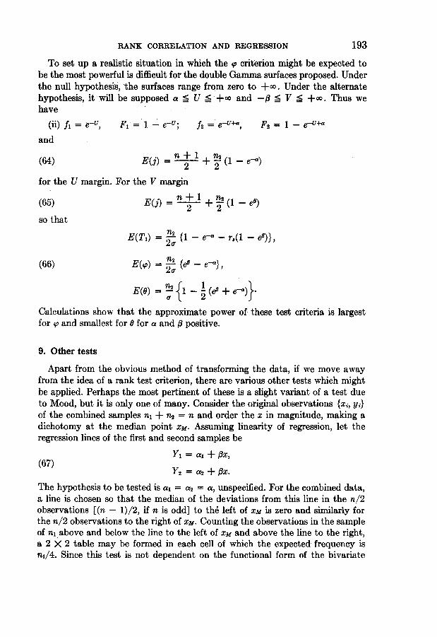
Calculations show that the approximate power of these test criteria is largestfor so and smallest for 0 for a and # positive.

9. Other tests

Apart from the obvious method of transforming the data, if we move awayfrom the idea of a rank test criterion, there are various other tests which mightbe applied. Perhaps the most pertinent of these is a slight variant of a test dueto Mood, but it is only one of many. Consider the original observations {xi, yi}of the combined samples n1 + n2 = n and order the x in magnitude, making adichotomy at the median point XM. Assuming linearity of regression, let theregression lines of the first and second samples be

Yi = a, + Ox,(67) Y2 = a2 + AX.The hypothesis to be tested is a, = a2 = a, unspecified. For the combined data,a line is chosen so that the median of the deviations from this line in the n/2observations [(n - 1)/2, if n is odd] to the left of XM is zero and similarly forthe n/2 observations to the right of XM. Counting the observations in the sampleof ni above and below the line to the left of XM and above the line to the right,a 2 X 2 table may be formed in each cell of which the expected frequency isn,/4. Since this test is not dependent on the functional form of the bivariate


distribution of the population from which ni + n2 = n observations have beendrawn, there seems to be no advantage in applying the same idea to the ranksof the x and the y. The only difficulty in application will lie in the choice of theline. This can be formidable if the number of observations is large.From recent work on the power function of test criteria based on ranked and

ordered variables, it would appear possible that tests more powerful than thosediscussed here could be obtained if, instead of the ranks, the equivalent normaldeviate of the rank is used. It is proposed to discuss tests based on the equivalentnormal deviate in a subsequent paper after further investigation of the powerfunctions of the tests proposed here.We would like to acknowledge stimulating criticism from colleagues, in par-

ticular from C. L. Mallows. Barbara Snow constructed the randomization dis-tributions.

10. Numerical appendix

As an illustration of the type of data which originally suggested the problemwe give here the precipitation in inches for two areas in southern California forthe two years 1957 and 1958. The experiments to determine the efficacy of cloudseeding operations of which this is part of the numerical data have been describedelsewhere, and also the statistical analysis used. Table VI shows the precipita-tion for one target area and one comparison area, seeded and not seeded. Theyears 1957 and 1958 are kept separate because in 1958 seeding operations were

TABLE VI

PRECIPITATION IN INCHES

1957 1958

(Not Seeded in Ventura) (Seeded in Ventura)

Seeded in S.B. Not Seeded in S.B. Seeded in S.B. Not Seeded in S.B.

Target Comparison Target Comparison Target Comparison Target Comparison

1.035 0.500 0.212 0.120 0.775 0.730 0.325 0.0600.000 0.000 0.265 0.220 1.232 0.250 1.635 1.4000.198 0.190 0.100 . 0.110 0.000 0.000 1.128 0.6900.235 0.470 0.152 0.090 1.428 0.090 0.335 0.1400.005 0.000 0.180 0.100 0.558 0.240 0.785 0.0300.445 0.140 0.015 0.000 2.740 2.990 0.482 0.0000.312 0.100 1.682 1.500 0.010 0.000 0.258 0.0400.070 0.000 0.002 0.000 0.055 0.030 0.972 2.5100.148 0.060 0.688 0.560 0.948 0.010 0.785 2.2100.000 0.000 0.072 0.000 0.358 0.020 0.162 0.0400.062 0.430 0.302 0.440 0.320 0.150 0.772 0.8601.728 0.440 0.008 0.060 0.142 0.060 0.022 0.0000.008 0.000 2.655 0.430

0.358 0.290


TABLE VII

RANKED PRECIPITATIONS

1957 1958

(Not Seeded in Ventura) (Seeded in Ventura)

Seeded in S.13. Not Seeded in S.. Seeded in S.B. Not Seeded in S.B.

Target Comparison Target Comparison Target. Comparison Target Comparison

23 23 16 15 16 21 9 11.51.5 4.5 18 18 22 17 24 23

15 17 11 14 1 2.5 21 2017 22 13 11 23 13 10 144 4.5 14 12.5 14 16 17.5 7.5

21 16 7 4.5 26 26 13 2.520 12.5 24 2.5 2 2.5 7 9.59 4.5 3 4.5 4 7.5 20 2512 9.5 22 24 19 5 17.5 241.5 4.5 [ 10 4.5 11.5 6 1 6 9.58 19 19 20.5 8 15 15 22

25 20.5 5.5 9.5 5 11.5 3 2.55.5 4.5 25 19

*11.5 18

26

24 x

22

!!20 *

.18 A

_16 x

o 14 xx

g12 -

x~~~~fL8 ~ / * * Seeded in Santo Barbara

x x Not Seeded in Santa Barbara1957 Not Seeded in Ventura

t4 / x

2

0

0 2 4 6 8 10 12 14 16 18 20 22 24 26

Ranked Precipitation for Comparison Area

FiGURE 3(a)

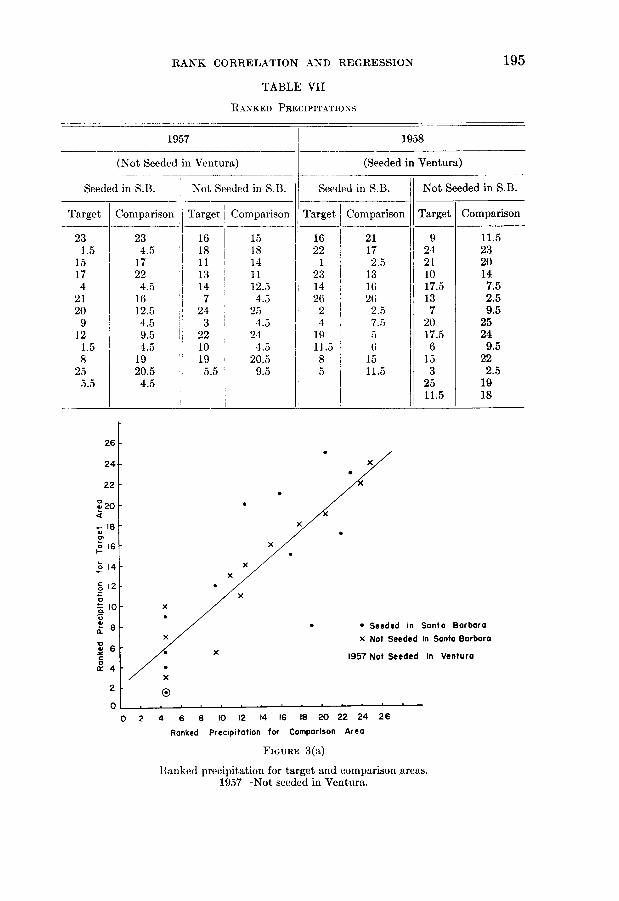
Ranked precipitation for target anld comparison areas.1957-Not seeded in Ventura.


also taking place in other areas. For each-year the target precipitations (seededand not seeded) are ranked and similarly the comparison precipitations. Theties were ranked by giving each observation in the tie the midrank. Subsequentcalculations showed it to be immaterial whether this procedure was adopted or

26 Sx

24 - x

22 -

I~~~~~~~~~~r20 _

:§,18 ' x X

16 *0 x /14-

° 12 . / x* 10 x

X 8 0

56 - x* Seeded In Santa BarbaraX Not Seeded In Santa Borbara

x 1958 Seeded In Ventura2

0 . . . . . .

0 2 4 6 8 10 12 14 16 18 20 22 24 26Ranked Precipitotion for Comparlson Area

FIGURE 3(b)

Ranked precipitation for target and comparison areas.1958-Seeded in Ventura.

the procedure of assigning a random order to the observations within the tie.The ranked observations are given in table VII. These results are shown graph-ically in figures 3(a) and 3(b). The rank regression lines of target area (y) oncomparison area (x) are

1957: y - 13 = 0.8532 (x - 13),

1958: y - 13.5 = 0.6799 (x - 13.5).

The null hypothesis is that there is no effect due to seeding so that one regres-sion line represents the true state of affairs. The alternate hypothesis is thatseeding is effective so that there are two regression lines, one for seeded and onefor nonseeded, with the seeded line lying parallel to but above that of thenonseeded. It is clear that either T* or s will be the appropriate criterion to use.

If Ryi and Rx, are the ranks of the target and comparison precipitation for theseeded area, then


T = 1 E [(R -i_ n + _ r8 (R- n + 1)],

(68) P = n (Ryi R.),

2 (n - n1) (1-r2), =n (n n1)1 n1(n -1) n(Substitution from the tabulated ranks gives the results shown in table VIII.The conclusion is that the tests have failed to detect increase of precipitationdue to seeding operations.

TABLE VIII

22Year T, I1/ alT/*0,

1957 -0.0056 0.1023 0.0053 0.1063 -0.055 0.0501958 0.0269 0.1584 0.094 0.1728 0.170 0.546

REFERENCES

[1] E. C. FIELLER, H. 0. HARTLEY, and E. S. PEARSON, "Tests for rank correlation coefficients.I," Biometrika, Vol. 44 (1957), pp. 470-481.

[2] M. G. KENDALL, "Rank and product moment correlation," Biometrika, Vol. 36 (1949),pp. 177-193.

[3] P. A. P. MORAN, "Rank correlation and product moment correlation," Biometrika, Vol. 35(1948), pp. 203-206.

[4] E. C. RHODES, "On a certain skew correlation surface," Biometrika, Vol. 14 (1922),pp. 355-377.

[5] E. S. PEARSON and H. 0. HARTLEY, Biometrika Tables for Statisticians, Vol. 1, Cambridge,Cambridge University Press, 1954.

[6] R. M. SUNDRUM, "A method of systematic sampling based on order properties," Bio-metrika, Vol. 40 (1953), pp. 452-456.

[7] M. J. VAN UVEN, "Extension of Pearson's probability distributions to two variables, I,II, III, IV," Nederl. Akad. Wetensch. Proc., Ser. A, Vol. 50 (1947), pp. 1063-1070, 1252-1264. Vol. 51 (1948), pp. 41-52, 191-196.

RANK CORRELATION AND REGRESSION IN ......RANK CORRELATION AND REGRESSION 179 difficult to choose...

Documents

Transcript of RANK CORRELATION AND REGRESSION IN ......RANK CORRELATION AND REGRESSION 179 difficult to choose...