Vessel and cargo motions - TU Delft
160
Vessel and cargo motions A frequency domain method to study combined vessel and cargo responses A.J. van der Heiden
Transcript of Vessel and cargo motions - TU Delft

Vessel and cargomotions
A frequency domain method to studycombined vessel and cargo responses
A.J. van der Heiden


Vessel andcargo motions
A frequency domain method to studycombined vessel and cargo responses
by
A.J. van der Heidento obtain the degree of Master of Science
at the Delft University of Technology,to be defended publicly on Friday September 20, 2019 at 10:00 AM.
Student number: 4213580Project duration: November 9, 2018 – September 20, 2019Thesis committee: Dr. Ir. P.R. Wellens, Delft University of Technology, chairman
Dr. -Ing. S. Schreier, Delft University of Technology, supervisorDr. Ir. M.B. Duinkerken, Delft University of TechnologyIr. A. Vreeburg, BigLift Shipping, supervisorMSc PhD A. van Deyzen, Royal HaskoningDHV
An electronic version of this thesis is available at http://repository.tudelft.nl/.


Contents
List of Figures vList of Tables ixPreface xiAbstract xiii1 Introduction 1
1.1 BigLift Shipping . . . . . . . . . . . . . . . . . . . . . . . . . . . . . . . . . . . . . . . . . . 11.1.1 Heavy Lift Market . . . . . . . . . . . . . . . . . . . . . . . . . . . . . . . . . . . . . 11.1.2 Company Profile . . . . . . . . . . . . . . . . . . . . . . . . . . . . . . . . . . . . . . 1
1.2 Problem Statement . . . . . . . . . . . . . . . . . . . . . . . . . . . . . . . . . . . . . . . . 21.3 Origin of the Problem Statement . . . . . . . . . . . . . . . . . . . . . . . . . . . . . . . . . 3
1.3.1 Lifting Operations . . . . . . . . . . . . . . . . . . . . . . . . . . . . . . . . . . . . . 31.3.2 Waves during Lifting Operations . . . . . . . . . . . . . . . . . . . . . . . . . . . . . . 31.3.3 Control of Cargo Motions . . . . . . . . . . . . . . . . . . . . . . . . . . . . . . . . . 4
1.4 Elaboration of the problem statement . . . . . . . . . . . . . . . . . . . . . . . . . . . . . . 41.5 Objectives. . . . . . . . . . . . . . . . . . . . . . . . . . . . . . . . . . . . . . . . . . . . . 61.6 Approach . . . . . . . . . . . . . . . . . . . . . . . . . . . . . . . . . . . . . . . . . . . . . 6
1.6.1 Multi-Body System. . . . . . . . . . . . . . . . . . . . . . . . . . . . . . . . . . . . . 61.6.2 Frequency Domain . . . . . . . . . . . . . . . . . . . . . . . . . . . . . . . . . . . . 71.6.3 Model Layout . . . . . . . . . . . . . . . . . . . . . . . . . . . . . . . . . . . . . . . 7
1.7 Thesis layout . . . . . . . . . . . . . . . . . . . . . . . . . . . . . . . . . . . . . . . . . . . 8
2 Theoretical Background 92.1 Multi-Body Dynamics. . . . . . . . . . . . . . . . . . . . . . . . . . . . . . . . . . . . . . . 92.2 Hydrodynamic Background . . . . . . . . . . . . . . . . . . . . . . . . . . . . . . . . . . . . 112.3 Pendulum Motions . . . . . . . . . . . . . . . . . . . . . . . . . . . . . . . . . . . . . . . . 152.4 Linearized Spring Values . . . . . . . . . . . . . . . . . . . . . . . . . . . . . . . . . . . . . 172.5 Influence of Damping. . . . . . . . . . . . . . . . . . . . . . . . . . . . . . . . . . . . . . . 172.6 Natural Frequency, Phase Difference and Resonance . . . . . . . . . . . . . . . . . . . . . . . 182.7 Natural Frequencies of Multi-Body Systems. . . . . . . . . . . . . . . . . . . . . . . . . . . . 202.8 Nonlinearities. . . . . . . . . . . . . . . . . . . . . . . . . . . . . . . . . . . . . . . . . . . 24
3 Model description 253.1 Model Layout . . . . . . . . . . . . . . . . . . . . . . . . . . . . . . . . . . . . . . . . . . . 253.2 Vessel Input . . . . . . . . . . . . . . . . . . . . . . . . . . . . . . . . . . . . . . . . . . . . 263.3 Crane and Cargo Model . . . . . . . . . . . . . . . . . . . . . . . . . . . . . . . . . . . . . . 293.4 Mooring Lines Input . . . . . . . . . . . . . . . . . . . . . . . . . . . . . . . . . . . . . . . 343.5 Cargo Control Systems . . . . . . . . . . . . . . . . . . . . . . . . . . . . . . . . . . . . . . 383.6 Motion Calculations . . . . . . . . . . . . . . . . . . . . . . . . . . . . . . . . . . . . . . . 443.7 Significant Motions . . . . . . . . . . . . . . . . . . . . . . . . . . . . . . . . . . . . . . . . 463.8 Verification . . . . . . . . . . . . . . . . . . . . . . . . . . . . . . . . . . . . . . . . . . . . 473.9 Validation . . . . . . . . . . . . . . . . . . . . . . . . . . . . . . . . . . . . . . . . . . . . . 543.10 Parameter Influence . . . . . . . . . . . . . . . . . . . . . . . . . . . . . . . . . . . . . . . 56
3.10.1 Cargo Mass . . . . . . . . . . . . . . . . . . . . . . . . . . . . . . . . . . . . . . . . 573.10.2 Crane Cable Length . . . . . . . . . . . . . . . . . . . . . . . . . . . . . . . . . . . . 583.10.3 Crane Top Z Position . . . . . . . . . . . . . . . . . . . . . . . . . . . . . . . . . . . . 583.10.4 Crane Top Y Position . . . . . . . . . . . . . . . . . . . . . . . . . . . . . . . . . . . . 583.10.5 Crane Top X Position . . . . . . . . . . . . . . . . . . . . . . . . . . . . . . . . . . . . 583.10.6 Vessel Draught . . . . . . . . . . . . . . . . . . . . . . . . . . . . . . . . . . . . . . . 59
iii
iv Contents
3.10.7 Vessel Metacentric Height . . . . . . . . . . . . . . . . . . . . . . . . . . . . . . . . . 59
4 Baseline Calculations 614.1 Baseline Case . . . . . . . . . . . . . . . . . . . . . . . . . . . . . . . . . . . . . . . . . . . 614.2 Wave Direction . . . . . . . . . . . . . . . . . . . . . . . . . . . . . . . . . . . . . . . . . . 634.3 Natural Frequencies and Eigenvectors . . . . . . . . . . . . . . . . . . . . . . . . . . . . . . 654.4 Baseline Behaviour . . . . . . . . . . . . . . . . . . . . . . . . . . . . . . . . . . . . . . . . 66
5 Sensitivity of lifting variables 715.1 Influences of Lifting Variables. . . . . . . . . . . . . . . . . . . . . . . . . . . . . . . . . . . 71
5.1.1 Cargo Mass . . . . . . . . . . . . . . . . . . . . . . . . . . . . . . . . . . . . . . . . 725.1.2 Crane Cable Length . . . . . . . . . . . . . . . . . . . . . . . . . . . . . . . . . . . . 735.1.3 Crane Top Z Position . . . . . . . . . . . . . . . . . . . . . . . . . . . . . . . . . . . . 745.1.4 Crane Top Y Position . . . . . . . . . . . . . . . . . . . . . . . . . . . . . . . . . . . . 755.1.5 Crane Top X Position . . . . . . . . . . . . . . . . . . . . . . . . . . . . . . . . . . . . 765.1.6 Vessel Draught . . . . . . . . . . . . . . . . . . . . . . . . . . . . . . . . . . . . . . . 785.1.7 Metacentric Height . . . . . . . . . . . . . . . . . . . . . . . . . . . . . . . . . . . . 805.1.8 Results of Lifting Variable Influence Study . . . . . . . . . . . . . . . . . . . . . . . . . 80
5.2 Influence of Mooring Lines . . . . . . . . . . . . . . . . . . . . . . . . . . . . . . . . . . . . 83
6 Cargo control systems 896.1 Stiffness via tugger winches . . . . . . . . . . . . . . . . . . . . . . . . . . . . . . . . . . . . 90
6.1.1 Polypropylene wires . . . . . . . . . . . . . . . . . . . . . . . . . . . . . . . . . . . . 906.1.2 Steel wires . . . . . . . . . . . . . . . . . . . . . . . . . . . . . . . . . . . . . . . . . 94
6.2 Location of tugger winches . . . . . . . . . . . . . . . . . . . . . . . . . . . . . . . . . . . . 976.3 Passive compensation. . . . . . . . . . . . . . . . . . . . . . . . . . . . . . . . . . . . . . . 1016.4 Active damping . . . . . . . . . . . . . . . . . . . . . . . . . . . . . . . . . . . . . . . . . . 1046.5 Results . . . . . . . . . . . . . . . . . . . . . . . . . . . . . . . . . . . . . . . . . . . . . . 108
7 Discussion 1098 Conclusion 111Bibliography 115A Free body diagrams 117
A.1 Free body diagrams crane cable connection . . . . . . . . . . . . . . . . . . . . . . . . . . . 117A.2 Free body diagrams mooring line connection . . . . . . . . . . . . . . . . . . . . . . . . . . . 120A.3 Free body diagrams cargo control system connection. . . . . . . . . . . . . . . . . . . . . . . 122
B Matrices 127C Equations ofMotion 131D RAOs 137E Working principle passive heave compensation 139
E.1 Passive Compensation . . . . . . . . . . . . . . . . . . . . . . . . . . . . . . . . . . . . . . 139E.2 Active compensation . . . . . . . . . . . . . . . . . . . . . . . . . . . . . . . . . . . . . . . 142

List of Figures
1.1 Three different vessels of BigLift Shipping. . . . . . . . . . . . . . . . . . . . . . . . . . . . . . . . . 2
2.1 Matrix quadrant visualization . . . . . . . . . . . . . . . . . . . . . . . . . . . . . . . . . . . . . . . . 112.2 Illustration that a sum of many simple regular waves makes an irregular sea[12][32] . . . . . . . 112.3 Illustration of a regular wave[20] . . . . . . . . . . . . . . . . . . . . . . . . . . . . . . . . . . . . . . 122.4 Illustration of the composition of a wave spectrum [5] . . . . . . . . . . . . . . . . . . . . . . . . . 132.5 Definition of ship motions in six degrees of freedom[12] . . . . . . . . . . . . . . . . . . . . . . . . 142.6 Schematic pendulum mechanics . . . . . . . . . . . . . . . . . . . . . . . . . . . . . . . . . . . . . . 162.7 Load elongation curves of different mooring line materials[6] . . . . . . . . . . . . . . . . . . . . . 172.8 Influence of damping on the resonance and natural frequency [33] . . . . . . . . . . . . . . . . . 182.9 Influence of damping on the resonance and natural frequency. recreated from Katsuhiko Ogata
[25] . . . . . . . . . . . . . . . . . . . . . . . . . . . . . . . . . . . . . . . . . . . . . . . . . . . . . . . 192.10 Argand diagrams for different driving frequencies. . . . . . . . . . . . . . . . . . . . . . . . . . . . 202.11 Schematic of a double pendulum used in the example calculation of the natural frequencies
and eigenvectors [18] . . . . . . . . . . . . . . . . . . . . . . . . . . . . . . . . . . . . . . . . . . . . . 222.12 Illustration of the two eigenvectors of a double pendulum . . . . . . . . . . . . . . . . . . . . . . . 232.13 Linearized tension values of active tugger winches[19] . . . . . . . . . . . . . . . . . . . . . . . . . 24
3.1 Schematic drawing off the mathematical model that is created for this study. . . . . . . . . . . . 263.2 Representation of the influence of small and large rotations of the cargo on the crane cable
configuration . . . . . . . . . . . . . . . . . . . . . . . . . . . . . . . . . . . . . . . . . . . . . . . . . 303.3 Free body diagram of the interaction between the vessel and cargo via the crane cable for the
vessel surge motion and the vessel roll motion. These free body diagrams can be used to explainthe influence of these degree of freedom on other degrees of freedom in the multi-body system 32
3.4 Load elongation curves of different mooring line materials[6] . . . . . . . . . . . . . . . . . . . . . 353.5 Free body diagram of the interaction between the vessel and the shore via the mooring lines for
the vessel surge motion and the vessel roll motion. These free body diagrams can be used toexplain the influence of these degree of freedom on other degrees of freedom in the multi-bodysystem . . . . . . . . . . . . . . . . . . . . . . . . . . . . . . . . . . . . . . . . . . . . . . . . . . . . . 36
3.6 Free body diagram of the interaction between the vessel and the cargo via the cargo controlsystems for the vessel surge motion and the vessel roll motion. These free body diagrams canbe used to explain the influence of these degree of freedom on other degrees of freedom in themulti-body system . . . . . . . . . . . . . . . . . . . . . . . . . . . . . . . . . . . . . . . . . . . . . . 42
3.7 Response Amplitude Operators of the vessel six degrees of freedom for different mathematicalmodules of the Python tool . . . . . . . . . . . . . . . . . . . . . . . . . . . . . . . . . . . . . . . . . 46
3.8 Response Amplitude Operators of the vessel six degrees of freedom comparison of the calcula-tion done by Shipmo and the Python tool . . . . . . . . . . . . . . . . . . . . . . . . . . . . . . . . . 48
3.9 Eigenvector values of the two natural frequencies with a large influence on the vessel roll motionthat occur in the multi-body model. The first natural frequency occurs around r ad/s andthe second natural frequency occurs around r ad/s. . . . . . . . . . . . . . . . . . . . . . . . 49
3.10 Response Amplitude Operators of the vessel six degrees of freedom for a comparison of theconnection of the cargo. A comparison is made between the method where the weight of thecargo is attached to the crane top and a method where the cargo is modelled as a pendulum . . 50
3.11 Response Amplitude Operators of the cargo surge and sway motion for a comparison of theconnection of the cargo. A comparison is made between the method where the weight of thecargo is attached to the crane top and a method where the cargo is modelled as a pendulum . . 51
3.12 JONSWAP spectra for different wave periods and peak enhancement factors. The wave heightis equal to 1 meter for all wave spectra. . . . . . . . . . . . . . . . . . . . . . . . . . . . . . . . . . . 51
v

vi List of Figures
3.13 Response spectra of the vessel motions. The responses are calculated for waves according toJONSWAP spectra with a period of 12 and 16 seconds and a peak enhancement factor of 1.0. . . 53
3.14 Unfiltered responses of the Cargo Sway motion in the crane similator. The waves have an angleof 90 degrees relative to the vessel. The significant wave height is 1 meter and the period is 12seconds. . . . . . . . . . . . . . . . . . . . . . . . . . . . . . . . . . . . . . . . . . . . . . . . . . . . . 54
3.15 Filtered responses of the Cargo Sway motion in the crane similator. The second order waveforces are filtered a high pass-filter with a cutoff frequency of 120 seconds. The waves have anangle of 90 degrees relative to the vessel. The significant wave height is 1 meter and the periodis 12 seconds. . . . . . . . . . . . . . . . . . . . . . . . . . . . . . . . . . . . . . . . . . . . . . . . . . 55
3.16 JONSWAP spectra for different periods and peak enhancement factors. Hs is equal to 1 meterfor all spectra . . . . . . . . . . . . . . . . . . . . . . . . . . . . . . . . . . . . . . . . . . . . . . . . . 56
3.17 schematic of the vessel’s metacentric height [39] . . . . . . . . . . . . . . . . . . . . . . . . . . . . 59
4.1 Side view and top view drawing of the BigLift Shipping vessel Happy Sky . . . . . . . . . . . . . . 61
4.2 Crane curves of the BigLift Shipping vessel Happy Sky . . . . . . . . . . . . . . . . . . . . . . . . . 62
4.3 Influence of different wave angles on the vessel roll motion and cargo sway motion RAO . . . . . 64
4.4 Influence of different wave angles on the vessel pitch motion and cargo surge motion RAO . . . 64
4.5 Influence of different wave angles on the vessel surge motion RAO. . . . . . . . . . . . . . . . . . 64
4.6 Eigenvectors of natural frequencies 2 till 6 of the baseline model . . . . . . . . . . . . . . . . . . . 66
4.7 RAO of the vessel roll motion with the baseline variable values . . . . . . . . . . . . . . . . . . . . 67
4.8 A detailed vessel roll motion RAO for frequencies between and 0.55 /s and betweenand rad/s . . . . . . . . . . . . . . . . . . . . . . . . . . . . . . . . . . . . . . . . . . . . . . . . . 67
4.9 RAO of the cargo sway motion with the baseline variable values . . . . . . . . . . . . . . . . . . . 67
4.10 A detailed cargo sway motion RAO for frequencies between and rad/s and betweenand rad/s . . . . . . . . . . . . . . . . . . . . . . . . . . . . . . . . . . . . . . . . . . . . . . 68
4.11 Phase of the vessel roll and cargo sway motion for the different frequencies within the range inwhich the RAOs are calculated. The Phases are calculated for the responses of the multi-bodymodel with the baseline variables . . . . . . . . . . . . . . . . . . . . . . . . . . . . . . . . . . . . . 69
4.12 Phase of the wave excitation force in vessel the vessel sway and vessel roll direction. . . . . . . . 69
4.13 JONSWAP spectra for different wave periods. The wave periods are varied between 12 and 16seconds. The wave height is set to 1 meter and the peak enhancement factor is equal to 1. . . . 70
4.14 Response spectra of the vessel roll and cargo sway motion for waves with a period of 12, 14and 16 seconds. The Phases are calculated for the responses of the multi-body model with thebaseline variables . . . . . . . . . . . . . . . . . . . . . . . . . . . . . . . . . . . . . . . . . . . . . . . 70
5.1 Relation between cargo mass and the natural frequencies of the roll and pendulum motions . . 73
5.2 Relation between crane cable length and the natural frequencies of the roll and pendulum mo-tions . . . . . . . . . . . . . . . . . . . . . . . . . . . . . . . . . . . . . . . . . . . . . . . . . . . . . . . 74
5.3 Relation between crane top Z position and the natural frequencies of the roll and pendulummotions . . . . . . . . . . . . . . . . . . . . . . . . . . . . . . . . . . . . . . . . . . . . . . . . . . . . . 75
5.4 Relation between crane top Y position and the natural frequencies of the roll and pendulummotions . . . . . . . . . . . . . . . . . . . . . . . . . . . . . . . . . . . . . . . . . . . . . . . . . . . . . 76
5.5 Relation between crane top X position and the natural frequencies of the roll and pendulummotions . . . . . . . . . . . . . . . . . . . . . . . . . . . . . . . . . . . . . . . . . . . . . . . . . . . . . 77
5.6 Relation between the vessel draught with a relative cargo mass and the natural frequencies ofthe roll and pendulum motions . . . . . . . . . . . . . . . . . . . . . . . . . . . . . . . . . . . . . . . 79
5.7 Relation between vessel draught with a constant cargo mass and the natural frequencies of theroll and pendulum motions . . . . . . . . . . . . . . . . . . . . . . . . . . . . . . . . . . . . . . . . . 79
5.8 Relation between vessel GM and the natural frequencies of the roll and pendulum motions . . . 80
5.9 Sketch of the mooringline configuration of table 5.12 . . . . . . . . . . . . . . . . . . . . . . . . . . 84
5.10 Influence of different mooring line configurations on the vessel roll motions. The different con-figurations are combinations of the lines in table 5.12 . . . . . . . . . . . . . . . . . . . . . . . . . 84
5.11 Influence of different mooring line configurations on the cargo sway motions. The differentconfigurations are combinations of the lines in table5.12 . . . . . . . . . . . . . . . . . . . . . . . 85

List of Figures vii
5.12 Eigenvector value comparison between the multi-body system without mooring lines and themulti-body system with a stiff mooring line configuration, configuration 3 in figures 5.10 and5.11. The natural frequency that is compared is the natural frequency at r ad/s. . . . . . . . 86
5.13 Eigenvector value comparison between the multi-body system without mooring lines and themulti-body system with a stiff mooring line configuration, configuration 3 in figures 5.10 and5.11. . The natural frequency that is compared is the natural frequency at r ad/s. In thisfigure the eigenvector values of the vessel roll and cargo sway motion are neglected . . . . . . . 86
5.14 Eigenvector values of the natural frequency found at r ad/sthat appears when a stiff moor-ing line configuration is used . . . . . . . . . . . . . . . . . . . . . . . . . . . . . . . . . . . . . . . . 87
6.1 Influence of tugger winches on the vessel roll motion and cargo sway motion RAOs for a fre-quency between and r ad/s. The stiffness of the tugger ropes is varried between 20and 40 kN /m. . . . . . . . . . . . . . . . . . . . . . . . . . . . . . . . . . . . . . . . . . . . . . . . . . 91
6.2 Influence of tugger winches on the vessel roll motion and cargo sway motion RAOs for a fre-quency between and r ad/s. The stiffness of the tugger ropes is varried between 20and 40 kN /m. . . . . . . . . . . . . . . . . . . . . . . . . . . . . . . . . . . . . . . . . . . . . . . . . . 91
6.3 Jonswap spectra for different wave periods. The wave periods are varied between 12 and 16seconds. The wave height is set to 1 meter and the peak enhancement factor is equal to 1. . . . 92
6.4 Influence of tugger winches on the vessel roll motion and cargo sway motion RAOs for a fre-quency between and r ad/s. The stiffness of the tugger ropes is varried between 20and 40 kN /m. . . . . . . . . . . . . . . . . . . . . . . . . . . . . . . . . . . . . . . . . . . . . . . . . . 93
6.5 Influence of tugger winches on the vessel roll motion and cargo sway motion RAOs for a fre-quency between and r ad/s. The stiffness of the tugger ropes is varried between 20and 40 kN /m. . . . . . . . . . . . . . . . . . . . . . . . . . . . . . . . . . . . . . . . . . . . . . . . . . 93
6.6 Eigenvector of the natural frequency that occurs when steeltugger wires are used. The naturalfrequency can be seen in figure 6.8a . . . . . . . . . . . . . . . . . . . . . . . . . . . . . . . . . . . . 95
6.7 Influence of tugger winches on the vessel roll motion and cargo sway motion RAO for a fre-quency between and r ad/s. The stiffness of the tugger ropes is varried between 4000and 10000 kN /m. . . . . . . . . . . . . . . . . . . . . . . . . . . . . . . . . . . . . . . . . . . . . . . . 95
6.8 Influence of tugger winches on the vessel roll motion and cargo sway motion RAO for a fre-quency between and r ad/s. The stiffness of the tugger ropes is varried between 4000and 10000 kN /m. . . . . . . . . . . . . . . . . . . . . . . . . . . . . . . . . . . . . . . . . . . . . . . . 96
6.9 Influence of tugger winches on the vessel roll motion and cargo sway motion RAO for a fre-quency between and r ad/s. The stiffness of the tugger ropes is varried between 4000and 10000 kN /m. . . . . . . . . . . . . . . . . . . . . . . . . . . . . . . . . . . . . . . . . . . . . . . . 97
6.10 Influence of the tugger winch configuration on the vessel roll motion RAO. Configurations ofthe tugger winches are given in table 6.6 . . . . . . . . . . . . . . . . . . . . . . . . . . . . . . . . . 99
6.11 Influence of the tugger winch configuration on the cargo sway motion RAO. Configurations ofthe tugger winches are given in table 6.6 . . . . . . . . . . . . . . . . . . . . . . . . . . . . . . . . . 99
6.12 Influence of the tugger winch configuration on the vessel pitch motion RAO. Configurations ofthe tugger winches are given in table 6.6 . . . . . . . . . . . . . . . . . . . . . . . . . . . . . . . . . 99
6.13 Influence of the tugger winch configuration on the cargo surge motion RAO. Configurations ofthe tugger winches are given in table 6.6 . . . . . . . . . . . . . . . . . . . . . . . . . . . . . . . . . 100
6.14 Eigenvector of the natural frequency of r ad/s for the multi-body system with the thirdtugger winch configuration. The tugger winch configurations are given in table 6.6 . . . . . . . . 100
6.15 Eigenvector of the natural frequency of r ad/s for the multi-body system with the thirdtugger winch configuration. The tugger winch configurations are given in table 6.6 . . . . . . . . 101
6.16 Influence of damping applied via tugger winches on the vessel roll motion RAO. The dampingof the tugger ropes is varied between 5% and 15% of ξ. . . . . . . . . . . . . . . . . . . . . . . . . . 102
6.17 Influence of damping applied via tugger winches on the cargo sway motion RAO. The dampingof the tugger ropes is varied between 5% and 15% of ξ. . . . . . . . . . . . . . . . . . . . . . . . . . 102
6.18 Influence of damping applied via tugger winches on the vessel roll motion RAO. The stiffness ofthe tugger wires is set to 30kN /m and the damping is varied between 100 and 400 kN /m/s . . . 105
6.19 Influence of damping applied via tugger winches on the cargo sway motion RAO. The stiffnessof the tugger wires is set to 30kN /m and the damping is varied between 10 and 30 kN /m/s . . . 105

viii List of Figures
6.20 Influence of damping applied via tugger winches on the vessel roll motion response spectra.The stiffness of the tugger wires is set to 30kN /m and the damping is varied between 100 and400 kN /m/s. The wave spectra used is a Jonswap spectra with Tp = 14 s and γ = 1.0 . . . . . . . 106
6.21 Influence of damping applied via tugger winches on the cargo sway motion response spectra.The stiffness of the tugger wires is set to 30kN /m and the damping is varied between 100 and400 kN /m/s. The wave spectra used is a Jonswap spectra with Tp = 14 s and γ = 1.0 . . . . . . . 106
A.1 The two free body diagrams of the interaction between the vessel and cargo via the crane cableor the surge motion of the vessel and the sway motion of the vessel . . . . . . . . . . . . . . . . . 117
A.2 The two free body diagrams of the interaction between the vessel and cargo via the crane cablefor the heave motion of the vessel and the roll motion of the vessel . . . . . . . . . . . . . . . . . . 118
A.3 The two free body diagrams of the interaction between the vessel and cargo via the crane cablefor the pitch motion of the vessel and the yaw motion of the vessel . . . . . . . . . . . . . . . . . . 118
A.4 The two free body diagrams of the interaction between the vessel and cargo via the crane cablefor the surge motion of the cargo and the sway motion of the cargo . . . . . . . . . . . . . . . . . 119
A.5 The free body diagram of the interaction between the vessel and cargo via the crane cable forthe heave motion of the vessel and the roll motion of the vessel . . . . . . . . . . . . . . . . . . . . 119
A.6 The two free body diagrams of the interaction between the vessel and the shore via mooringlines for the surge motion of the vessel and the sway motion of the vessel . . . . . . . . . . . . . . 120
A.7 The two free body diagrams of the interaction between the vessel and the shore via mooringlines for the heave motion of the vessel and the roll motion of the vessel . . . . . . . . . . . . . . 120
A.8 The two free body diagrams of the interaction between the vessel and the shore via mooringlines for the pitch motion of the vessel and the yaw motion of the vessel . . . . . . . . . . . . . . 121
A.9 The two free body diagrams of the interaction between the vessel and the cargo via cargo controlsystems for the surge motion of the vessel and the sway motion of the vessel . . . . . . . . . . . . 122
A.10 The two free body diagrams of the interaction between the vessel and the cargo via cargo controlsystems for the heave motion of the vessel and the roll motion of the vessel . . . . . . . . . . . . 123
A.11 The two free body diagrams of the interaction between the vessel and the cargo via cargo controlsystems for the pitch motion of the vessel and the yaw motion of the vessel . . . . . . . . . . . . 123
A.12 The two free body diagrams of the interaction between the vessel and the cargo via cargo controlsystems for the surge motion of the cargo and the sway motion of the cargo . . . . . . . . . . . . 124
A.13 The two free body diagrams of the interaction between the vessel and the cargo via cargo controlsystems for the heave motion of the cargo and the roll motion of the cargo . . . . . . . . . . . . . 124
A.14 The two free body diagrams of the interaction between the vessel and the cargo via cargo controlsystems for the pitch motion of the vessel and the yaw motion of the cargo . . . . . . . . . . . . . 125
D.1 Comparison between the influence of different wave angles on the vessel RAOs . . . . . . . . . . 137D.2 Comparison between the influence of different wave angles on the cargo RAOs . . . . . . . . . . 137
E.1 Schematic drawing of a passive heave compensator . . . . . . . . . . . . . . . . . . . . . . . . . . 140E.2 Schematic drawing of tugger winches applied to cargo in a crane . . . . . . . . . . . . . . . . . . . 143E.3 Schematics of a winch based active heave compensator. For simplicity the crane dynamics is
neglected. The stationary sheave represents the crane tip[[42] . . . . . . . . . . . . . . . . . . . . 144
List of Tables
3.1 Values exported from Shipmo hydrodynamic database . . . . . . . . . . . . . . . . . . . . . . . . . 283.2 Input values needed to calculate pendulum stiffness matrix . . . . . . . . . . . . . . . . . . . . . . 333.3 Input values needed to calculate the mooring line stiffness matrix . . . . . . . . . . . . . . . . . . 383.4 Input values needed to calculate the damping and stiffness matrices for damping systems . . . 443.5 Most probable maximum comparison where the RAOs are constant and the wave height is varied 543.6 Most probable maximum comparison between crane simulator and python tool . . . . . . . . . 553.7 Variables changed to study the influence . . . . . . . . . . . . . . . . . . . . . . . . . . . . . . . . . 57
4.1 Values of the variables used in the baseline case. . . . . . . . . . . . . . . . . . . . . . . . . . . . . 634.2 Natural frequencies of the baseline multi-body system . . . . . . . . . . . . . . . . . . . . . . . . . 654.3 MPM values of the vessel roll and cargo sway motion for baseline variables. The wave height is
taken equal to 1 meter. . . . . . . . . . . . . . . . . . . . . . . . . . . . . . . . . . . . . . . . . . . . . 70
5.1 Variables changed to study the influence . . . . . . . . . . . . . . . . . . . . . . . . . . . . . . . . . 725.2 Influence of cargo mass on the roll and pendulum natural frequencies and amplitude of the
resonance peaks. . . . . . . . . . . . . . . . . . . . . . . . . . . . . . . . . . . . . . . . . . . . . . . . 735.3 Influence of crane cable length on the roll and pendulum natural frequencies and amplitude of
the resonance peaks. . . . . . . . . . . . . . . . . . . . . . . . . . . . . . . . . . . . . . . . . . . . . . 745.4 Influence of the crane top Z position on the roll and pendulum natural frequencies and ampli-
tude of the resonance peaks. . . . . . . . . . . . . . . . . . . . . . . . . . . . . . . . . . . . . . . . . 755.5 Influence of the crane top Y position on the roll and pendulum natural frequencies and ampli-
tude of the resonance peaks. . . . . . . . . . . . . . . . . . . . . . . . . . . . . . . . . . . . . . . . . 765.6 Influence of the crane top X position on the roll and pendulum natural frequencies and ampli-
tude of the resonance peaks. . . . . . . . . . . . . . . . . . . . . . . . . . . . . . . . . . . . . . . . . 775.7 Influence of the crane top X position on the cargo surge natural frequency and amplitude of the
resonance peak. . . . . . . . . . . . . . . . . . . . . . . . . . . . . . . . . . . . . . . . . . . . . . . . . 785.8 Influence of the vessel draught with relative cargo mass on the roll and pendulum natural fre-
quencies and amplitude of the resonance peaks. . . . . . . . . . . . . . . . . . . . . . . . . . . . . 795.9 Influence of the vessel draught with a constant cargo mass on the roll and pendulum natural
frequencies and amplitude of the resonance peaks. . . . . . . . . . . . . . . . . . . . . . . . . . . . 795.10 Influence of the vessel’s metacentric height on the vessel roll and cargo sway natural frequency
and amplitude of the resonance peak. . . . . . . . . . . . . . . . . . . . . . . . . . . . . . . . . . . . 805.11 Variables changed to study the influence . . . . . . . . . . . . . . . . . . . . . . . . . . . . . . . . . 825.12 Different mooring line configurations used to calculate the influence of mooring lines on the
vessel and cargo respones. . . . . . . . . . . . . . . . . . . . . . . . . . . . . . . . . . . . . . . . . . 83
6.1 The coordinates of the tugger winches used in the influence calculations of the tugger winch . . 896.2 Natural frequency comparison between different stiffness values of the tugger wire. The first
and second natural frequency are given in radians per second and per second. . . . . . . . . . . 916.3 Most probable maximum comparison between different stiffness values of the tugger wire. The
MPMs are calculated for swell waves with a period of 12, 14 and 16 seconds. . . . . . . . . . . . . 946.4 Natural frequency comparison between different stiffness values of the tugger wire. . . . . . . . 966.5 Most probable maximum comparison between different stiffness values of the tugger wire. The
MPMs are calculated for swell waves with a period of 12, 14 and 16 seconds. . . . . . . . . . . . . 966.6 Three different tugger winch configurations used to calculate the influence of the tugger winch
configuration. . . . . . . . . . . . . . . . . . . . . . . . . . . . . . . . . . . . . . . . . . . . . . . . . . 976.7 Natural frequency comparison between different stiffness values of the tugger wire. The first
and second natural frequency are given in radians per second and per second. . . . . . . . . . . 101
ix

x List of Tables
6.8 Most probable maximum comparison between different tugger winch configurations. The tug-ger winch configurations can be found in table 6.6. The MPMs are calculated for swell waveswith a period of 12, 14 and 16 seconds. . . . . . . . . . . . . . . . . . . . . . . . . . . . . . . . . . . 101
6.9 Natural frequency comparison between different dampin values of the tugger wire. The tuggerwire stiffness used in the calculations is 30 kN. The MPMs are calculated for swell waves with aperiod of 12, 14 and 16 seconds. . . . . . . . . . . . . . . . . . . . . . . . . . . . . . . . . . . . . . . 103
6.10 Most probable maximum comparison between different critical damping values of the tuggerwire. The tugger wire has a stiffness of 30 kN. The MPMs are calculated for swell waves with aperiod of 12 seconds. . . . . . . . . . . . . . . . . . . . . . . . . . . . . . . . . . . . . . . . . . . . . . 103
6.11 Most probable maximum comparison between different critical damping values of the tuggerwire. The tugger wire has a stiffness of 30 kN. The MPMs are calculated for swell waves with aperiod of 14 seconds. . . . . . . . . . . . . . . . . . . . . . . . . . . . . . . . . . . . . . . . . . . . . . 103
6.12 Most probable maximum comparison between different critical damping values of the tuggerwire. The tugger wire has a stiffness of 30 kN. The MPMs are calculated for swell waves with aperiod of 16 seconds. . . . . . . . . . . . . . . . . . . . . . . . . . . . . . . . . . . . . . . . . . . . . . 104
6.13 Most probable maximum comparison between different damping values and a stiffness valueof 30 kN /m. The damping has been varied between 100 kN /m/s and 400 kN /m/s. The swellwaves have a period of 12 seconds. . . . . . . . . . . . . . . . . . . . . . . . . . . . . . . . . . . . . . 107
6.14 Most probable maximum comparison between different damping values and a stiffness valueof 30 kN /m. The damping has been varied between 100 kN /m/s and 400 kN /m/s. The swellwaves have a period of 14 seconds. . . . . . . . . . . . . . . . . . . . . . . . . . . . . . . . . . . . . . 107
6.15 Most probable maximum comparison between different damping values and a stiffness valueof 30 kN /m. The damping has been varied between 100 kN /m/s and 400 kN /m/s. The swellwaves have a period of 16 seconds. . . . . . . . . . . . . . . . . . . . . . . . . . . . . . . . . . . . . . 107
C.1 Definition of abbreviations used in the equations of motion . . . . . . . . . . . . . . . . . . . . . . 131

Preface
The final project that a student has to fulfill before he can graduate is his master thesis. This report is the resultof my master thesis to complete the Master’s program Marine technology at Delft University of Technology.The specialisation of my master is ship hydromechenics. The project has been carried out on behalf of BigLiftShipping. At BigLift Shipping I have been a graduation intern at the Engineering department.
Let me start with showing my gratitude for the graduation committee. Dr. Ir. P.R. Wellens, thank you forstepping in as the chair during the last phase of my master project. Ir. M.B. Duinkerken thank you for takingthe time to take part of the committee. Dr. Ir. S. Schreier, thank you very much for all the time you spend tohelp me during my research. Thank you for all the knowledge you shared and the questions that pushed meto think in other directions. Your questions also helped me to go back to the principles of the problem.
I also want to express my appreciation to BigLift Shipping. The Engineering department for providing mewith a place to work and all the advice I got. Thank you Anne Vreeburg and Gerardo Rodriguez Conde foryour daily supervision. Thank you for all the times you helped me with guidance and valuable feedback.
I would like to thank my family. I will start with my parents, Ben and Carla. Thank you for the endless supportand your open arms. Thank you for teaching me to always try my hardest. Maarten, my elder brother, thankyou for all your advice.
The next words are reserved for my friends. Thank you all for the welcome distraction from studying. Fromsailing in the J22 and SB20, Studying in Trondheim and all other activities we did together. Thank you Jorenfor all the, somewhat longer, coffee talks we had during our study days in Delft. Thank you all for making mystudy time the amazing time it was.
Finally I would like to thank Lisanne. Thank you for all your love and patience. Thank you for your reassuringwords on the moments I got home tired and the moments I was really busy. Even on the moments I wantedto procrastinate writing the thesis or preparing my presentation.
A.J. van der HeidenDelft, September 2019
xi


Abstract
When lifting operations are performed by a heavy lifting vessel, the motions of the vessel and cargo are pre-dicted by conventional six degrees of freedom calculations. It is assumed that the cargo is attached to thecrane top in order to decrease the stability of the vessel and perform accurate calculations. While these con-ventional calculations can be used to calculate the vessel motions and the motions of the crane top, the cargomotions are not taken into account. In conventional calculations the dynamical aspects of the cargo are nottaken into account and the forces due to cargo motions are neglected.
In several recent projects carried out by BigLift Shipping swell waves have presented BigLift Shipping withchallenges. Due to these swell waves the vessel and cargo where excited which caused problems during theselifting operations. Therefore BigLift Shipping is intrested in a method to calculate the vessel motions in com-bination with the cargo motions.
There are two objectives of the research presented in this report. The first objective is to increase knowledge ofthe dynamical effects of the cargo on the vessel motions and vice versa. The second objective of this researchis to investigate if it is possible to reduce the cargo motions during lifting operations by changing variables ina lifting plan or by controlling the cargo with cargo control systems. To fulfill both objectives a tool is created.
The tool that is created is a mathematical model of the vessel and cargo body. In this model the vessel andcargo are modelled as a multi-body system and is based on the frequency domain. A multi-body frequencydomain model is able to calculate the responses of both the vessel and cargo motions quickly. For the inputof the model the vessel constraints of the vessel and cargo body with each other and the outside world hasto be described in a mathematical way. The constraints can be divided over four different modules. Thefirst module of constraints follow from the vessel hydrodynamics. The connection of the cargo to the vesselvia the crane cable are described in the second module. The influences of mooring lines on the multi-bodysystem are described in the third module. Lastly the influences of cargo control systems are described in thefourth module. With the different modules the influence of variables of a lifting operation on the vessel andcargo motions can be studied. The output of the tool consists of the vessel RAOs. Together with wave spectracalculations these RAOs can be translated to response spectra and most probable maximum values.
The tool that is created is used to fulfill the two research objectives. First a set of calculations are done todetermine the baseline responses of the multi-body system. Different variables of a lifting operation arevaried and the influence of the cargo mass, crane cable length, crane top position, vessel draught and vesselmetacentric height are studied. This study showed that these variables can have a large influence on theresponses and natural frequencies of the multi-body system. Cargo control systems are also implemented inthe multi-body model. Calculations that included cargo control systems showed that the increased stiffnessof such systems can vary the natural frequencies of the different degrees of freedom in the multi-body model.When damping is applied via cargo control systems the most probable maximum values of the motions canbe reduced with maximum of 55.3%.
xiii


1Introduction
BigLift Shipping is a heavy lifting transport company. The company transports heavy cargo all over the world.Most of BigLift’s vessels are equipped with two heavy lifting cranes and these cranes are used to lift cargoeson-board and of-board of a vessel. Lately BigLift Shipping experiences problems during lifting operationsdue to swell waves. When swell waves occur at lifting operations, the cargo hanging in the crane can start tooscillate which can cause an unsafe work environment. BigLift Shipping is interested in the origin of thesemotions. When the origion of these motions is understood a possible solution can be studied.
In this report a study regarding the influence of heavy cargo hanging in a vessel crane is studied, as well aspossible reduction methods are presented. This report is the result of a study carried out at BigLift Shippingwith supervision of Delft University of Technology. To start this research first the profile of BigLift Shippingis explained in section 1.1. In section 1.2 the problem statement is worked out followed by the origin ofthis problem statement in section 1.3. Thereafter the problem statement is elaborated in section 1.4. Theobjectives are discussed in section 1.5 and the approach of the study is given in section 1.6. Lastly the thesislayout is explained in section 1.7.
1.1. BigLift ShippingBigLift Shipping is the company where this project is carried out. As explained in the introduction BigLiftShipping transports heavy cargo. In this section the heavy lifting marked and company profile of BigLiftShipping are worked out.
1.1.1. Heavy Lift MarketBigLift Shipping mainly operates in the heavy lifting market. The heavy lifting market is a market in whichlifting operations with cargoes between 60 and 60.000 mton are executed for the purpose of transportation.Cargoes lighter than this weight are not considered as heavy lift cargoes and heavier cargoes are not common,although possible with newer vessels. There are a lot of different heavy lift companies around the world.However, since the range of cargo weights in heavy lifting is large, the amount of different specializations isalso large. For semi-submersible vessels the lifting capacity is almost equal to the deadweight of the vessel.The largest single hull semi-submersible, the Boka Vanguard, can lift up to 117.000 ton. The largest doublehull semi-submersible crane vessel in the world, the Heerema Sleipnir, can lift cargoes up to 18.000 mton andthe largest single hull crane vessel, the Zhen Hua 30, can lift op to 12.000 mton. However, these large cranevessels are mainly designed for the lifting operation and are not designed to transport the lifted cargo. Whilethe large heavy lifting crane vessels are not designed to transport the cargo the design can be fully focusedon the lifting operation itself. These vessels have methods to increase their stability and reduce the motionsof the vessel. Vessels that also need to transport their cargo cannot be optimized in such a way, reducing thelifting capabilities of the vessel.
The heavy lift transport vessels are operating in a complete new market but the largest limitations of the heavylift transport vessels are the capacity of the on board cranes. Therefore it is common to express the capacityof a heavy lift vessel in the maximum lifting weight of the crane instead of the of the maximum deadweight ofthe vessel. BigLift competes with Jumbo and SAL Heavy Lift in this market.
1.1.2. Company ProfileBigLift Shipping is a heavy lift transportation company that currently operates with a fleet of 21 heavy liftvessels and 4 heavy transport vessels. The largest heavy lift vessel is the Happy Star with a combined liftingcapacity of 2200 mton. The smallest vessel type has a combined lifting capacity of 800 mton. The 4 heavytransport vessels are not equipped with cranes and use the roll on, roll off method. In figure 1.1 three differentvessel types are shown.
1

2 1. Introduction
The company’s head office can be divided in two departments. The commercial department and operationaldepartment. The head office is located in Amsterdam and BigLift has smaller offices all over the world withlocal agents. In the head office all the orders and bookings that are inquired worldwide are taken care of.The operational department handles all requirements for a smooth operation from stowage possibilities toloading arrangements and stability calculations.
(a) BigLift’s Happy Star, the largestheavy lifting vessel of BigLift
Shipping
(b) Biglift’s Happy-D type vessel. A vesselwith 2 cranes of 400 mton and 1 crane of
120 mton.
(c) BigLift’s Happy Buccaneer. BigLiftsoldest, still sailing vessel operating in a
remote location
Figure 1.1: Three different vessels of BigLift Shipping.
1.2. Problem StatementBigLift Shipping is a heavy lift shipping company with 21 heavy lift vessels and 4 heavy transport vessels. Allthe heavy lift vessels are equipped with 2 or more cranes. The lifting capacity of the cranes vary between 400mton safe working load for the smaller vessels up to 1100 mton safe working load per crane. The cranes onboard of the vessel can also operate in tandem lifts increasing the lifting capacity to 800 mton and 2200 mtonrespectively. The deadweight of the largest vessel is equal to 19.000 mton. This means that the lifting capacityof the largest vessel is equal to 5.5 % of the vessels deadweight in single lift operations. Which is a considerableamount. In tandem lift operations the cargo can have a weight equal to 11 % of the vessels deadweight.
The heavy lift vessels transport the cargoes all over the world. The loading operations also take place all overthe world, from the North Sea to the Gulf of Mexico to the far East and Australia. Due to this variation in load-ing sites the environmental conditions of each loading operation is different. The environmental conditionsinfluence the motions of the vessel and cargo during lifting operation.
In several recent projects carried out by BigLift Shipping swell has presented BigLift with challenges. Althoughusually BigLift contracts states that the loading / discharge berth shall be “Always Safe” and “Swell Free”, inpractice BigLift is facing swell affected ports from time to time. Working in swell poses safety issues sincethe cargo will be set in motion due to the vessel response. This problem from a shipping company is theorigin of this study. BigLift is considering swell as the not modifiable cause of the problem. However, sinceswell waves are an external factor all waves can be researched during this study. Mooring configurationsare considered part of the vessel’s configuration. Although mooring arrangements are dependent on theloading location the mooring arrangements are mechanically a part of the vessel configurations. Thereforemooring arrangements should not be restricting factors in the research. The parts that can be modified, tosome extend, are the vessel and cargo properties. Therefore the influence of waves on and the interactionbetween vessel and cargo motions must be studied. The results of this study can be used to increase the timein which lifting operations are feasible and safe.
The problem of this study can be described by one problem statement, which is shown below.
Problem statement:
"Determine the influence of vessel motions and cargo motions on each other during lifting operations in wavesand develop a method to decrease the motions during these lifting operations in waves"
This problem statement contains several different aspects. These different aspects will be worked out in thefollowing sections.

1.3. Origin of the Problem Statement 3
1.3. Origin of the Problem StatementIn this section the problem statement and the origin are further explained. This is done by splitting the prob-lem in different elements. Firstly the lifting operation process is detailed by explaining the sequence of eventsin a lifting operation.
1.3.1. Lifting OperationsLifting operations are executed to lift cargo from shore on board of the vessel or the other way around. Car-goes can also be lifted on or from barges or other vessels next to the heavy lifting vessel. Heavy cargoes aredifficult to manage during the lifting operation. The cargoes are vulnerable or voluminous which creates noroom for errors. During the lifting operation and slewing of the cranes the stability and draught of the vesselhas to be controlled. The stability and draught of the vessel can be controlled by pumping water in and outof the different ballast tanks of the vessel. A lifting operation from shore to ship can be divided in five stages.These stages are listed with a small explanation below.
• Free flotation: Free flotation is the condition of the vessel before the lifting operation starts. The vesseland cargo are not yet connected to each other. Thus they do not influence each other yet.
• Pretension: During this part of the lifting operation the cargo is connected to the vessel. The mechan-ical connection via the crane cable couples the two bodies to each other.
• Free hanging - Above shore:At this point the cargo is lifted from the ground. While the cargo is hangingabove the shore/barge, the outreach of the crane is relative large. The cargo can swing like a pendulum.These swinging motions should be limited to prevent clashes between the cargo and its surroundingobjects. The swinging motions of the cargo will also create a load on the vessel which is another reasonwhy the cargo swinging motions must be limited.
• Free hanging - Above vessel: When the crane rotates the cargo above deck the outreach of the crane isrelative small. Reducing some of the loads on the vessel due to the outreach of the crane. The cargo canstill swing like a pendulum which can damage the cranes or cargo holds of the vessel when the cargo islowered on deck.
• Put down: Placing the cargo on deck. The relative motions between the vessel and cargo determinehow difficult this stage is. This stage is critical while clashes between the vessel and cargo will damageboth the cargo and vessel bodies.
The largest vessel of BigLift Shipping can lift cargoes up to 5.5% of their deadweight with a single lift operation.This percentage goes up to 11 % for tandem lift operations where two cranes are used. Since the distancebetween the centre of gravity of the vessel and the crane tip is much larger than the metacentric height of thevessel, large loads due to cargo motions can occur. Large motions of the cargo in the crane can also cause acollision between the cargo and the vessel crane’s or hold or make it impossible to put down the cargo safelyon shore or on the vessel’s deck. Therefore the cargo motions must be kept small during lifting operations.
The vessel and cargo bodies are interconnected due to the coupling via the crane cable. Due to this couplingthe vessel and cargo motions are coupled to each other. When waves excite the vessel hull, the vessel hullis not the only body that is excited by the waves. The cargo itself has no direct connection with the waves.However indirectly the cargo will also translate by the waves via the connection between the vessel and thecargo. The relation between the cargo and vessel motions must be determined in a mathematical way beforethe influence of waves can be calculated.
1.3.2. Waves during Lifting OperationsWhen waves ’hit’ the hull of a vessel or other floating object energy is transferred from this wave to the vesselor object. The energy that is transferred will set the vessel into motion.
As stated before BigLift contracts states that the loading / discharge berth shall be "Always Safe" and "SwellFree". However this is not always the case during lifting operations. Most operations take place behind break-waters which reduces the waves around the vessel during lifting operations. However breakwaters will notnullify all waves. Large waves can move past smaller breakwaters and a residue of the waves will still enterthe loading site. At the same time swell waves, waves with a relative large period, also tend to move pastbreakwaters.

4 1. Introduction
The most common waves during lifting operations are swell waves. Swell waves are waves that find theirorigin by distant weather systems. The weather at the lifting location do not influence the swell waves them-selves. Swell waves often have a long period which also means that they have a long wave length. These waveswith a long wave length tend to have a lot of energy in them which can be transferred to vessel motions. Swellwaves also tend to move past breakwaters easier than waves generated by local weather, also called sea waves.
Since swell waves tend to occur more often during lifting operations than sea waves the main objective isto investigate the influence of swell waves. However, since a tool is being generated to solve the problemstatement the tool is designed in such a way that sea waves can also be investigated with the tool. Sine everyport or loading site has its own influence on the wave patterns that occur the influences of the ports, quaysand bays on waves is not studied. Basic wave patterns are assumed in the calculations.
When BigLift operates in remote or offshore locations breakwaters are not installed. Here waves will be evenlarger than the waves in protected areas for the same weather conditions. Thus waves can occur during alllifting operations. These waves will influence the lifting operations and limit the operational window of liftingoperations. The influence of waves on both the vessel and cargo motions must be studied before a solutionto these motions can be proposed.
The waves at different locations can influence the vessel and cargo motion in such a way that these liftingoperations become unsafe and dangerous for both the people performing the lifting operation and the ob-jects used during and located around the lifting operation. When it is unsafe to perform the lifting operationmust be stopped until safer work environments occur. These delays are a problem for the project of whichthe lifting operation is part of but severe delays can also be a problem for upcoming projects while the vesselcannot start these projects before finishing the current project.
1.3.3. Control of Cargo MotionsDuring lifting operations the cargo can swing like a pendulum. This causes problems in handling the cargoin a safe way. One way to control the cargo motions is by creating fixed connections between the cargoand the vessel. When these connections are made the cargo can not move away from its relative positionto the vessel’s centre of gravity. However, during lifting operations the cargo must be transferred from onelocation to another location. This does also mean that it is impossible to create fixed connections betweenthe vessel and cargo while the distance between the cargo and the vessel’s centre of gravity does change.Therefore a fixed connection between the vessel and cargo is not possible. However, when one end of thefixed connection is connected to a winch-like machine the connection can be controlled. This could make itpossible to move the cargo with the crane as long as the winches are controlled to move along with the crane.These winches are called tugger winches. However, such connections will also transfer forces between thevessel and cargo which can create other dangerous situations.
To reduce the motions in a system the kinetic energy needs to be extracted from the multi-body system.In other dynamical problems dampers are used to reduce the motions of certain bodies. A common usedexample is the use of shock-absorbers in cars. Shock-absorber transfers kinetic energy of the car into heat.This reduces the motions of the car. An other example is a damper placed between the mooring line andthe shore to reduce mooring forces. Such a method can also be used to reduce the forces transferred via thetugger wires.
Connections between the cargo and vessel will always introduce new dynamical relations between the twobodies. These relations will influence the relation between vessel and cargo motions. Therefore these rela-tions and their influence must be studied.
1.4. Elaboration of the problem statementAs stated in section 1.3.1 both the vessel and cargo will be excited by waves. In section 1.3.2 is explainedthat not all lifting sites will be swell free and section 1.3.3 is explained that there are methods to control thecargo. When these three aspects are combined it is clear that the waves that can be present at almost everylocation can influence the lifting operations. BigLift is facing problems due to swell more often than in thepast. Therefore BigLift is interested in a study to the combination of vessel and cargo motions during liftingoperations. In this study the influence of different vessel and cargo variables and cargo control systems willinvestigated.

1.4. Elaboration of the problem statement 5
The first part of the problem statement states: "Determine the influence of vessel and cargo motions on eachother during lifting operations". This parts covers the study with regards to the combined vessel and cargomotions. In this part of the problem statement the vessel and cargo motions are defined as the researchsubjects. In current or conventional calculations the cargo is seen as a part of the vessel itself and the cargocannot move independently from the vessel. This makes it possible to do some easy and quick calculationswith regards to the vessel motions when cargo is lifted in the cranes but the motions of the cargo and theinteraction between the vessel and cargo cannot be calculated. In the conventional calculations the freehanging cargo is accounted for but the dynamical swinging aspects of the cargo is not accounted for. Nopublic research is done with regards to the combined motions of the vessel and the cargo.
During lifting operations the cargo is coupled via the crane cable. First the physical constraints between thevessel and the cargo must be examined. These physical constraints have to be described in a mathematicalway in order to calculate the influence of both motions on each other. Third party multi-body dynamic soft-ware might solve the coupling between the vessel and the cargo but this software is probably not equippedwith tools to solve the hydrodynamic aspects of the physical problem. Therefore it is not useful to use third-party multi-body dynamics software and the constraints will be studied. Subsequently a mathematical toolwill be developed to calculate the vessel and cargo motions. The tool created can be used to determine thenatural frequencies of the vessel and cargo, but the tool can also be used to determinate the influence ofdifferent lifting configurations on the responses of the vessel and cargo.
The second part of the problem statement states "each other during lifting operations in waves". This partstates that the waves influence both the vessel and cargo motions. The influence of waves on both the vesseland cargo motions must be examined. Hydrodynamic properties of both the vessel and waves must be addedto the mathematical tool. The hydrodynamic properties of the vessel will describe how the vessel and cargomotions are influenced by the water and how the bodies are excited from wave forces. The waves will createexcitation forces that will both influence the vessel and cargo bodies. These forces follow from the hull shapeand loading properties of the vessel.
While swell waves have the largest influence on loading operations according to BigLift Shipping, the influ-ence of most wave types can be calculated in the same way. Therefore the calculations are created in sucha way that the influence of both sea waves and swell waves can be calculated and even waves with an evenhigher period. Wave spectra calculations can be used to calculate the influence of different types of waves onthe motions of the vessel and the cargo. The main focus will be on the swell waves with a period between 12and 16 seconds. However, in the tool that is created the influence of sea waves can also be calculated.
The last part of the problem statement states: "and develop a method to decrease the motions during liftingoperations in waves". As in every mechanical system there are excitation frequencies at which the bodies ofthe vessel and cargo show larger responses. This is called resonance and occurs around the natural frequencyof a mechanical system. The motions of the vessel and cargo that occur during lifting operations are depen-dent on the waves that occur during these lifting operations. When these wave excitate the vessel and cargoaround their natural frequency the responses of these bodies on the waves will be large. Different variablesof a lifting operation will influence the responses in different ways. Knowledge of this influence can be usedto chose lifting configurations that show smaller influences of the waves that occur during lifting operationsand reduce the responses of the vessel and cargo motions.
Another method to reduce the motions of the cargo is by introducing cargo control systems. Such systemsare briefly explained in section 1.3.3. Besides introducing a stiffer connection between the vessel and cargobodies damping can be introduced to transfer kinetic energy from the cargo into another kind of energy. Inthe tool created the constraints from a stiff connection between the vessel and cargo will be added as well asdamping. The influence of these two properties will be studied. From this study a method to decrease theresponses of the cargo on the waves can be created.

6 1. Introduction
1.5. ObjectivesThis reason this research is fulfilled can be traced back in three objectives. The first objective of the researchis to gain a better understanding of the vessel and cargo interactions. In this chapter it has been describeda number of times that there are no public methods to calculate the interaction between vessel and cargomotions. BigLift is sometimes hindered by cargo motions in such severe ways that the loading operations hasto be cancelled for a certain amount of time. Once the mutual relationship has been mapped BigLift engineerscan use this information to find solutions for these problems during lifting operations. When BigLift canoperate in more severe weather conditions the money loss due to delays will decrease.
The second objective is the tool itself. While the understanding of relations between the vessel and cargo isuseful for decision making by gut feeling or knowing which variables of a lifting configuration can be changedin order to influence the vessel and cargo motions, the tool itself can be used to calculate the exact influenceof such changes. The tool can be used in future projects to determine what the best lifting configuration is forthat project.
The third objective is to create a better understanding of the influence of cargo control techniques. Right nowsome techniques to control the cargo are known. However, public research on the effects is never done. Theexact influence of both a stiff connection and applied damping is not known at BigLift Shipping. Even if suchstudies are done by other companies the results are hidden and not available for public use. Therefore theinfluence of cargo control systems on both the amplitude of the responses as the form of the responses.
These three objectives can be combined in one thesis objective. This objective is given below: Develop a toolthat can calculate the coupled responses of both the vessel and cargo bodies on waves and use this tool to studythe influence of different lifting configurations and cargo control systems on the vessel and cargo responses.
To fulfill the thesis objective first the interaction between the vessel hull and waves will be determined. Thewave forces are the main excitation forces during lifting operations. From these forces the responses of boththe vessel and cargo can be calculated. The tool will be made modular that different input variables canbe studied at any given time without large alterations of the tool. When the tool is finished the tool can beused for different projects executed by BigLift Shipping to predict vessel and cargo motions during the liftingoperations of these projects.
1.6. ApproachNow that it is clear that some lifting operations can not be performed due to waves the approach to investigatethe problem and search for solutions can be described.
1.6.1. Multi-Body SystemThe motions that are studied are motions that occur during lifting operations. When a vessel is in transitthe cargo is seafastened and thus integrated with the vessel motions while the lashings keep the cargo inplace. During lifting operations the cargo hanging in a crane will act like a pendulum. The cargo can developmotions and through coupling these motions can increase or reduce the vessel motions. Therefore liftingoperations require other calculations than normal stability, seakeeping or hydrostatic calculations. In con-ventional calculations the cargo weight is attached to the crane tip during lifting operations. This will give anaccurate solution for simple stability calculations of the vessel. However, the interaction between the vesseland the cargo motions is not taken into account. The coupling of the cargo to the vessel via a crane cable mustbe modelled in a mathematical way that not only the influence of the cargo weight on the vessel motions istaken into account but also the influence of the motions of both bodies on each other is taken into account.
In this study the vessel and cargo will be seen as two separate bodies which can move independently fromeach other but are coupled through certain dynamical constraints. Due to these constraints forces are trans-ferred between the two bodies which will influence the responses of both bodies. The dynamical system ofthe vessel and its cargo are treated as a multi-body system. In multi-body systems the constraints are de-scribed via mathematical formulations. All the responses of the different bodies and directions the bodiescan move in are calculated at the same time. In this way the cargo and the vessel motions can be calculatedas a combined system. From this multibody system all or specific responses of both the vessel and cargo canbe extracted and studied.

1.6. Approach 7
The lifting operations that are considered can be lifting operations at sea or in a bay where no mooring linesare attached or at a quay where mooring lines are part of the calculations. Therefore the influence of mooringlines will also be studied. The influence of quays, ports and breakwaters on waves and thus wave forces isdifferent for every single location around the world. A study to wave patterns such as refraction and reflectionwill not be executed. The different wave patterns that can occur are assumed to be input values and thus notpart of the study goal.
1.6.2. Frequency DomainEquations of motion that consists of a time varying aspect that is also harmonic can be solved in the timedomain or in the frequency domain. When the equation of motion is solved in the time domain the equationof motion is solved directly for different time steps. E.g. the equation of motion is solved for every 0.1 second.The advantage of the time domain calculations is that the solutions contain the non-linear behaviour in theequation of motions. Mooring lines, tugger lines, low frequency drift forces, viscous damping and forces dueto wind and currents can cause these non-linear motions. In section 2.3 the equation for the pendulum mo-tions are described. When the pendulum is excited in the horizontal and vertical direction at the same timenon linear behaviour could also occur. This non-linear behaviour results in two, or more, natural frequen-cies. These natural frequencies follow from the different linear motions that form the non-linear pendulummotion. When the horizontal and vertical direction are considered as the two degrees of freedom two dif-ferent linear natural frequencies occur. The first natural frequency is related to the natural frequency in thehorizontal translation and the second natural frequency is related to the vertical translation. When the X, Yand Z directions are considered as the three different translations of the pendulum three different naturalfrequencies will form the non-linear motion from the three natural frequencies of the X, Y and Z translations.This combination of translations is called parametric excitation.
The disadvantage of a time domain calculation is that the model becomes complex, the results are statisticallyhard to interpret and the calculations are time consuming. Since time domain calculations are expensivein computational power and computation time the user must have a great understanding of the physicalproblem for efficient calculations. Since all these disadvantages are at odds with the goal of this project timedomain simulations are not the favourable solution method.
When the equations of motions are linearized in all different aspects the equations can be solved in the fre-quency domain. Since the forces and excitations are harmonic, which will be further elaborated in section2.2, only the different mass, damping and stiffness values must be linearized. The advantages of frequencydomain calculations are time efficiency, simple frequency calculations instead of time step calculations andeasy to interpret results. The calculations and derivations that have to be solved are fairly easy and statisticalformulations can be used to interpret the results. The biggest disadvantage of frequency domain calcula-tions is that non-linearity cannot be included in the calculations. All the different non-linear aspects of theequation of motion must be linearized. However, most non-linear aspects do not have a big influence onthe model since the non-linear motions are small or the influence is not in a frequency of interest. Whenthe influence of these non-linear aspects are small they could also be neglected. Wind induced motions areexpected to be small since low wind speeds are required to allow safe lifting operations. Some non-linearmotions will break down before large amplitudes are generated, such as sub-harmonic motions (Journee andMassie)[12] and for other non-linear aspects a linear model is sometimes available such as the Ikeda method[13] for the viscous damping.
1.6.3. Model LayoutTo solve the research question a model will be made. This model will be made in the mathematical programPython. Python[7] is a programming language that can be used to solve a series of equations and other orders.Therefore it is particularly suitable to solve the multi-body problem of vessel and cargo motions. In this modeldifferent parts need to be taken into account. First all the constrains and coupling terms between the vesselmotions and cargo motions must be described in a mathematical way. When all constraints of the multibodysystem are determined the response of the vessel and cargo due to wave forces can be calculated. Theseresponses can be used to study the influences of different lifting configurations and the influence of cargocontrol systems. how this is done is described in chapter 3

8 1. Introduction
To create a model that can be used for every single lifting operation the tool will be made modular. Thismeans that the different constraints can be implemented in a flexible way. For example: the mooring linescan be neglected with one single option. While the model is modular different lifting configurations can besolved in rapid succession of each other to calculate the influence of different loading configurations on thecombined vessel and cargo motions for all different projects.
1.7. Thesis layoutFirst the theoretical background will be explained in chapter 2. In this chapter the physics required to solvethe problem will be described. First multi-body dynamics will be explained. Multi-body dynamics are usedto calculate the responses of both the vessel and cargo at the same time. Thereafter the hydrodynamic prop-erties of both waves and the vessel will be described. As third the physical properties of mooring lines andlinearization of spring values are explained. The connection between the vessel and cargo via the crane ca-ble will be described as fourth followed by the influence of damping on multi-body systems. Thereafter thenatural frequency calculations and their properties and usefulness will be explained. The influence of non-linearities will be tackled in the last section of the theoretical background.
After the theoretical background the model will be described in chapter 3. First the layout of the model will beexplained. Thereafter the input of the vessel hydromechanics are explained. Next the mathematical couplingbetween the cargo and the vessel via the crane cable is explained. As fourth the mathematical modelling ofmooring lines are explained followed by the explanation of the modelling of the cargo control systems. Afterall these input properties the motion calculations are explained. Thereafter the calculations of significantmotions are worked out. After that the verification is explained followed by the validation of the model. Nextthe mathematical influence of lifting variables are worked out when the sensitivity study is explained.
In chapter 4 the baseline calculations that have been carried out are explained. These baseline calculationsare prepared for both the sensitivity of the lifting variables study and the cargo control system influence study.In this chapter first the baseline case is explained. After the case the chosen wave direction is explained.Thereafter the natural frequencies and eigenvectors of the baseline case are calculated and explained. Lastlythe behaviour of the baseline case in terms of RAOs and most probable maximum values are worked out.
The influence of the different variables during a lifting operation are studied in chapter 5. In this chapter firstthe influence of the cargo mass is calculated followed by the crane cable length. As third, fourth and fifththe influence of the Crane top in Z, Y and X direction are studied respectively. Thereafter the influence of thevessel draught is studied followed by the influence of the metacentric height. After all these different variablestudies the results are summarized. The influence of mooring lines on the multi-body system are also studiedin this chapter
In chapter 6 the influence of cargo control systems are studied. First the influence of tugger wires with a lowstiffness value is studied followed by a study of tugger wires with a high stiffness value. Thereafter the influ-ence of low amounts of damping are studied followed by the influence of large damping values. In chapter 7the study is discussed. Lastly in chapter 8 the conclusion is given.

2Theoretical Background
In this chapter the theoretical background required to solve the problem is described. Since the multi-bodysystem consist of of two bodies it is important to understand all the dynamics of the system before combiningall the different influences. The vessel and the cargo are two different bodies. However, both bodies are in-fluenced by external factors, themselves and each other. All these influences will be described in the sectionsin this chapter. But first multi-body dynamics must be described to understand how the different theoreticalinfluences can be translated to equations. In section 2.1 multi-body dynamics are explained. Thereafter Sec-tion 2.2 the influences of waves and the vessel’s hydrodynamic properties are explained. Next the dynamicsof a pendulum are explained in section 2.3. The influence of mooring lines and the linearization of spring val-ues are worked out in section 2.4. In section 2.5 the influence of damping on dynamical systems is explained.Thereafter the influence of natural frequencies and resonance is clarified in section 2.6 followed by the ex-planation of natural frequency calculations of multi-body systems in section 2.7. Lastly the nonlinearities areworked out in section 2.8.
2.1. Multi-Body DynamicsThe problem consists of two different bodies, the vessel and the cargo. Both bodies can move independentlybut are influenced by each other. To understand how the bodies are influenced first multi-body dynamicsmust be described. Multi-body dynamics are dependent on the amount of bodies in the system, the degreesof freedom per body and the interaction between the different degrees of freedom in the system. A body isconsidered to be a rigid or flexible part of a mechanical system. Examples of this are a single arm of a robot,a solid block and the weight of a pendulum. The different bodies in a multi-body system are connected toeach other or the world via constraints which restrict the relative motions, velocities or accelerations of thebodies. Examples of these constraints are a spring between two bodies or the ground, water around a vesselor air around a body hanging from a crane. The degree of freedom of a system is the number of independentmotions that the system which consists of. In other words it is the number of parameters in which the stateof a physical system can be described. For example the position of a single locomotive along a train trackhas one single degree of freedom since the body can only move alongside the rail track and the position ofthe body can be described by the distance travelled along the rail track. The position of a rigid body in theopen space, such as a vessel in water, will have six degrees of freedom. The six degrees of freedom containthree translations and three rotations. These six degrees of freedom will be further described in section 2.2.In multi-body dynamics it is important to determine if the translations and rotations of the different bod-ies are truly independent. A train consisting out of a train with a wagon consist out of two different bodiesbut those bodies have a solid connection between them which causes the bodies to be dependent on eachother. The locomotive cannot move without moving the wagon in the same direction with the same distance.This system consisting out of two different bodies does only have one single degree of freedom. Lastly theinteraction between the different degrees of freedom is important. These interactions are often coupled tothe constraints between two bodies or a body and the world. A spring connected between two bodies willtransmit a force to the two bodies when the relative distance between the two bodies changes. The differentconstraints in multi-body dynamics can be translated in an algebraic equation that defines the relative trans-lation or rotation, and their time derivatives, between the different degrees of freedom of a body, the differentbodies or a body and the world. For example, the force that a spring transfers to a body can simply be calcu-lated by multiplying the spring stiffness with the relative extension of the spring. The equations that describethe different constraints can be combined in one big system. When all the constraints that occur in a systemare combined in a mathematical model the interactions between the bodies and the world can be calculated.In multi-body dynamics is the dynamic behavior a result from the equilibrium of applied forces and changeof momentum. The applied forces in the system consist of external forces but also of forces resulting fromthe stiffness and damping in the system. Since the motions of both bodies and all degrees of freedom can be
9

10 2. Theoretical Background
calculated at the same time with multi-body dynamics, multi-body dynamics is a good method to calculatethe interaction between vessel and cargo motions.
Since multibody dynamics is essentially a combination of different mathematical equations the general lawsof nature do apply on multi-body systems in the same way as in single body dynamics. Therefore the lawsof motion described by Newton in "Principia Mathematica Philosophiae Naturalis" can be used. The secondlaw, which explains how the velocity of an object changes when it is subjected to an external force is the mostimportant one for this study and shown in equation 2.1. This equation can be extended with damping andspring terms to develop an equation of motion of a mass-spring-damper system as shown in equation 2.2. Inthis equation M contains the mass component of a body, B contains the damping component applied to abody and C stands for the stiffness that is applied to the body. x, x and x represent the displacement, velocityand acceleration of the body respectively. Lastly the external forces acting on the body are given by F . Theequation of motion that describes a mass-spring-damper system is important because the essentials of thisequation are the same as the essentials of multi-body dynamics. When the Mass, Damping and Stiffness com-ponents of the single body calculation are changed in matrices and the displacement, velocity, accelerationand force components are changed in vectors the multi-body equation is formed.
Since the frequency domain is used all properties in the equation are linear. Due to the linearity the superpo-sition principle can be used. The superposition principle states that for linear systems, the net response causedby two or more inputs, is the sum of the inputs each would have caused on its own[40]. In other words, alldifferent influences on the multi-body systems can be calculated separately and added together to solve thecombined influence on the multi-body system. This is useful since it makes it possible to calculate all differ-ent constraints separately. When all constraints are known and translated to a mathematical relation all thesemathematical relations can be combined to solve the responses of the multi-body system.
In equation 2.2 different aspects such as hydrodynamic spring terms and pendulum spring terms, can becombined as long as the different systems can be linearized. This makes the equation of motion very use-ful to calculate the influence of different lifting configurations and cargo control systems. Every part of themulti-body system, such as hydrodynamics of the vessel, cargo pendulum and cargo control systems can becalculated separately and simply added to the combined system or removed as long as the different degreesof freedom are used in the same order in each and every individual system.
m ·a = F (2.1)
M · x +B · x +C · x = F (2.2)
The ship and cargo system contains two bodies. Both bodies exist out of three translations and three rotationsthus the combined system will contain out of a twelve degree of freedom system as long as all degrees offreedom are independent from each other. Since there are no rigid connections between the vessel and thecargo all degrees of freedom in the system are independent. The crane cable is considered a spring, whichwill be further elaborated in section 2.3. Although this spring is very stiff the vessel and the cargo can havean independent translation. In this twelve degree of freedom system the first six degrees of freedom willdescribe the motions of the vessel and the last six degrees of freedom will describe the motions of the cargoin the crane. The twelve degree of freedom system will result in 12 by 12 matrices and vectors with a lengthof 12 components in the equation of motion. Since the first six degrees of freedom contain the translationsand rotations of the vessel and the last six degrees of freedom contain the cargo translations and rotations thematrices can be divided in four quadrants as shown in figure 2.1. The top left quadrant shows the influence ofthe vessel on itself. The top right quadrant shows the influence of vessel motions on the cargo swing motions.The bottom left quadrant represents the influence of cargo motions on the vessel motions and the influenceof cargo motions on itself are shown in the bottom right quadrant.
Throughout the report the numbers coupled to the different degrees of freedom will stay constant. The cor-responding numbers for each degree of freedom are explained below. In section 2.2 the degrees of freedomand their directions will be further elaborated.

2.2. Hydrodynamic Background 11
• x1 = Vessel Surge
• x2 = Vessel Sway
• x3 = Vessel Heave
• x4 = Vessel Roll
• x5 = Vessel Pitch
• x6 = Vessel Yaw
• x7 = Cargo Surge
• x8 = Cargo Sway
• x9 = Cargo Heave
• x10 = Cargo Roll
• x11 = Cargo Pitch
• x12 = Cargo Yaw
Figure 2.1: Matrix quadrant visualization
2.2. Hydrodynamic BackgroundTwo important hydrodynamic aspects in this multi-body system are vessel motions and ocean waves. Thevessel motions are important since the vessel motions are part of the multi-body system. Ocean wave theoriesare important because the theory explains how waves are formed and how the excitation force applied to avessel forms from this theory.
Figure 2.2: Illustration that a sum of many simple regular waves makes an irregular sea[12][32]
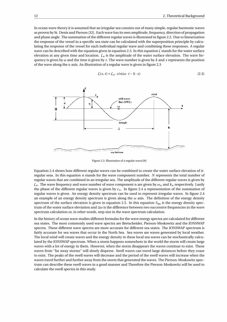
12 2. Theoretical Background
In ocean wave theory it is assumed that an irregular sea consists out of many simple, regular harmonic wavesas proven by St. Denis and Pierson [32]. Each wave has its own amplitude, frequency, direction of propagationand phase angle. The summation of the different regular waves is illustrated in figure 2.2. Due to linearizationthe response of the vessel in a specific sea state can be calculated with the superposition principle by calcu-lating the response of the vessel for each individual regular wave and combining these responses. A regularwave can be described with the equation given in equation 2.3. In this equation ζ stands for the water surfaceelevation at any given time and location. ζa is the amplitude of the water surface elevation. The wave fre-quency is given by ω and the time is given by t . The wave number is given by k and x represents the positionof the wave along the x-axis. An illustration of a regular wave is given in figure 2.3
ζ(x, t ) = ζa · si n(ω · t −k · x) (2.3)
Figure 2.3: Illustration of a regular wave[20]
Equation 2.4 shows how different regular waves can be combined to create the water surface elevation of ir-regular seas. In this equation n stands for the wave component number. N represents the total number ofregular waves that are combined in an irregular sea. The amplitude of the different regular waves is given byζn . The wave frequency and wave number of wave component n are given by ωn and kn respectively. Lastlythe phase of the different regular waves is given by εn . In figure 2.4 a representation of the summation ofregular waves is given. An energy density spectrum can be used to represent irregular waves. In figure 2.4an example of an energy density spectrum is given along the ω axis. The definition of the energy densityspectrum of the surface elevation is given in equation 2.5. In this equation Sηη is the energy density spec-trum of the water surface eleviation and ∆ω is the difference between two successive frequencies in the wavespectrum calculation or, in other words, step size in the wave spectrum calculation.
In the history of ocean wave studies different formulas for the wave energy spectra are calculated for differentsea states. The most commonly used wave spectra are Bretscheider, Pierson-Moskowitz and the JONSWAPspectra. These different wave spectra are more accurate for different sea states. The JONSWAP spectrum isfairly accurate for sea waves that occur in the North Sea. Sea waves are waves generated by local weather.The local wind will create waves and the energy density in these local sea waves can be stochastically calcu-lated by the JONSWAP spectrum. When a storm happens somewhere in the world the storm will create largewaves with a lot of energy in them. However, when the storm disappears the waves continue to exist. Thesewaves from "far away storms" will slowly disperse. Swell waves can travel large distances before they ceaseto exist. The peaks of the swell waves will decrease and the period of the swell waves will increase when thewaves travel further and further away from the storm that generated the waves. The Pierson-Moskowitz spec-trum can describe these swell waves in a good manner and Therefore the Pierson-Moskowitz will be used tocalculate the swell spectra in this study.

2.2. Hydrodynamic Background 13
ζ(x, t ) =N∑
n=1ζn · si n(ωn · t −kn x +εn) (2.4)
Sηη(ωn) = lim∆ω→0
0.5 ·ζ2n
∆ω(2.5)
Figure 2.4: Illustration of the composition of a wave spectrum [5]
In the introduction of this research is explained that this research will be focused on the vessel and cargobehaviour and that no study will be done with regards to the waves in ports and along side quays. Howeverthe superposition principle that makes it possible to model an irregular wave as a sum of many differentregular waves is very useful for the study of vessel and cargo motions. Since the wave dynamics can be splitup in regular waves the responses of a vessel can be calculated for regular waves. The response of a vesselin regular waves can than be translated to the response of a vessel in irregular waves by the use of the superposition principle of irregular waves. How the responses of a vessel can be calculated will be explained in thesecond half of this section.
In general 6 degrees of freedom are used when vessel motions are described. The degrees of freedom consistof out of three translations and three rotations. The three translations of the ship are translations acting on therigid body of the ship. The first translation is surge in the longitudinal x-direction where the positive directionis forwards. Sway is the second translation in lateral y-direction where the positive direction is a translation toport side. The third translation is in the vertical z-direction where upwards is the positive direction. The threerotations are rotations around the axis of the translation. The first rotation is roll about the x-axis. The rollmotion is expressed by φ. The pitch about the y-axis is the second rotation and expressed by θ. Yaw which isexpressed by ψ is the third rotation which is the rotation about the z-axis. All rotations are positive in a rightturning moment. Figure 2.5 shows the 6 degrees of freedom.
Besides the degrees of freedom of the vessel the degrees of freedom of the cargo are used in the multi-bodycalculations as described in section 3.1. In this section is also explained that the cargo degrees of freedom aregiven by number 7 till 12.

14 2. Theoretical Background
Figure 2.5: Definition of ship motions in six degrees of freedom[12]
The equation of motion that describes a mass-spring-damper system given in equation 2.2 is important be-cause vessel motions in waves can be translated to such a system. First order ship motions are sinusoidaloscillations, which can be described by linear equations of motion. Therefore linear behaviour is assumedin most calculations. This makes it possible to apply the superposition principle. The assumed linear sys-tems makes it possible to decompose hydrodynamic forces in mass, spring and damping coefficients. Sincethe motions of a vessel will move water, extra aspects must be taken into account in the equation of motion.This will be done by adding the added mass term and the potential damping term which describes the addedinertia due to the acceleration of water and the damping due radiation of water, which creates waves, respec-tively. Since not all damping forces are linear the viscous damping has to be introduced. The viscous damp-ing contains the linearized nonlinear damping coefficients for different wave frequencies and roll angles. Theequation of motion given in equation 2.2 can also be used to write down the hydrodynamical properties ofa vessel. This equation is given in equation 2.6. Matrices are given by uppercase boldface letters, vectors aregiven by lowercase boldface letters and scalars are given by lowercase, normal font letters. The letter i is usedto describe the imaginary unit. In the equation M and A represents the mass and added mass matrices of thevessel. The linear damping matrix is represented by B while Bv represents the linearized viscous damping.C is the spring matrix and x represents the displacement vector while x and x represent the first and secondderivation of x to time. The wave excitation force vector is given by Fexc . The force vector is given by a capitalletter. This is an exception on the notations used in this report. Since Fexc is an harmonic force proportionalto the incoming harmonic wave it can be assumed that Fexc = Fae iωt . Since Fexc is assumed to be harmonicx can also be assumed to have a form equal to x = xae−iωt since the response of the vessel is a direct responseon the wave excitation force. This assumption makes it possible to write x and x as a function of x as shownin equations 2.7 to 2.9.
(M + A) · x + (B +Bv ) · x +C · x = Fexc (2.6)
x = xae−iωt (2.7)
x =−iω · xae−iωt (2.8)
x =−ω2 · xae−iωt (2.9)
Equation 2.6 can be split in three essential parts. The first part is the wave excitation force. This is the externalforce applied to the system by the waves. The second part is the response of the vessel given by x and itsderivatives. From these vectors follow the motions of the vessel. The last major part in this equation is thecombined ship system. This system is the combination of the mass matrices, damping matrices and stiffnessmatrix and their relation to the wave frequency. The combined ship system S is given in equation 2.10. Theship system contains all dynamical connections between the different degrees of freedom in terms of mass,damping and stiffness. Note that this equation is a part of the left hand side of equation 2.2. This part isimportant since most of the time the vessel responses are calculated with the help of the ship system andthe excitation forces since the ship system and external excitation forces can be calculated independentlyas long as the hull form is known. Equation 2.11 shows how the response of a vessel due to waves can becalculated. This equation is basically equation 2.2 rewritten to solve the equation for x instead of F . In
2.3. Pendulum Motions 15
vessel hydrodynamics the response is given in[
maζa
]for translations and in
[φaζa
]for rotations and are called
Response Amplitude Operators, RAOs in short. ma represents the response of a translation in meters andφa represents the response of a rotation in degrees. The wave height in meters is given by ζa . The RAOs arethus translations or rotations per meter wave height. Since the RAOs are related to the wave height the RAOsdo not vary when the wave height changes. The RAOs are frequency dependent. Even though the RAOs areindependent of the wave height, non linearities in the multi-body system requires different RAO calculationsfor different amplitudes of the responses of the multi-body system. The responses are coupled to the waveheight and thus larger wave heights can cause different RAO calculations. An example is the viscous dampingthat is coupled to the vessels roll amplitude. Greater wave heights will increase the roll response of the vesseland thus a larger roll damping factor must be applied.
S =−ω2 · (M + A)− iω · (B +Bv )+C (2.10)
x = S−1Fexc (2.11)
The method for calculating the vessel responses for the six degree of freedom system can be expanded to thetwelve degree of freedom system. In section 2.1 is explained that multi-body dynamics is a combination ofsmaller equations. One of these smaller equations is the vessel hydrodynamic equation shown in equation2.6. Since this is one of the smaller equations that will be solved in the multi-body system the mass, addedmass, damping, viscous damping and stiffness matrices that describe the vessels hydrodynamic particularsas well as the wave excitation force can be substituted in the first six degrees of freedom of the multi-bodyequation.
Since it is assumed that the cargo will be lifted above water no hydrodynamic influences on the cargo mustbe calculated. This does also mean that there is no hydrodynamic coupling between the cargo and the vessel.As a result only the top left quadrant of the multi-body matrices illustrated in figure 2.1 will be filled withhydrodynamic properties. The wave excitation force vector will have non-zero entries in the first six entriesand all zero entries for the last six entries of the vector. This does not mean that the cargo will not move dueto wave forces but that the waves will not exert a force to the cargo directly. The cargo can still be movedindirectly due to coupling between the vessel and cargo responses.
2.3. Pendulum MotionsThe cargo in a crane can be assumed to move as a pendulum. The standard equation of motion as describedin equation 2.2 can be used to implement the pendulum motions in the multi-body system. The mass of thecargo is filled in on the diagonal of the mass matrix for the translations and the radii of inertia for the rotations.Besides air friction other form of damping are present in the pendulum system. These other forms of dampingare much smaller than the air friction and Therefore neglected. Examples of other forms of damping arerotational friction of the crane cable and an increase of heath in the cable due to friction. The air friction issmall but it will not be neglected because it is a form of natural damping on the pendulum, and even thoughit is small, in comparison with other forms of natural damping it is relatively large. For an accurate modeldamping needs to be applied, otherwise the responses of the degrees of freedom will give extremely largeexcitations around the natural frequency. The spring constant follows from the offset of the cargo to the cranetip and the restoring force induced by gravity. Figure 2.6 shows the schematic forces acting on the pendulumwhile the pendulum is in motion. Gravity applies a constant force Fg . This constant force applies tension onthe wire, shown as a T in the figure. When there is an offset between the crane tip and the cargo, an angle θwith regard to the vertical will exist and a horizontal component is introduced. This horizontal componentFr est can be calculated with equation 2.12. The offset ∆x can be calculated with equation 2.13. Where l isthe length of the crane wire. The angles of rotation are considered small since small motions are required forsafe lifting operations. Small motions is also a necessity for linearization. When small motions occur it canbe assumed that si nθ = θ and t anθ = θ. These assumptions can be done for θ < 10◦ This is justified sincethe cargo motions need to be small. When the motions are not small the linearization will not give accuratesolutions but the workability is also not sufficient. This assumption makes it possible to write the restoringforce as a function of the offset, this is shown in equation 2.14. The pendulum spring stiffness follows fromthe restoring force and is given in equation 2.15.

16 2. Theoretical Background
Figure 2.6: Schematic pendulum mechanics
Fr est = m · g · t anθ (2.12)
∆x = l · si nθ (2.13)
Fr est = m · g
l∆x (2.14)
Kp = m · g
l(2.15)
For mathematical purposes ∆x is explained as a function of l and θ in equation 2.13. However in the multi-body system θ will not be calculated. ∆x is the result of the relative response between the crane tip and thecentre of gravity of the cargo. The crane tip can move by translations of the vessel but rotations of the ves-sel will also cause a translation of the crane tip. When the vessel rolls the crane tip will not only rotate butalso show a translation. The distance between the centre of gravity of the vessel and the crane tip will causetranslations of the crane tip when the vessel rotates. The roll motion together with the vertical position of thecrane tip will result in a offset in y-direction. All the different aspects of the pendulum restoring stiffness andthe offset that causes a restoring force will be explained in section 3.3
Now that the horizontal restoring stiffness is known it is time to determine the vertical restoring stiffness.The vertical restoring stiffness follows from the Young’s modulus and the dimensions of the crane wire. Therestoring force of the crane wire is given in equation 2.16. Here the Young’s modulus is given with E. A rep-resents the cross-sectional area of the crane wire. The length of the crane wire is given with l and ∆z is theoffset in vertical direction. From the restoring force in vertical direction follows the vertical stiffness given inequation 2.17. The vertical offset ∆z is not only dependent on the vessel and cargo heave motions. Differentrotational motions will cause a vertical offset in the same way that these rotations do this in the calculationsfor the pendulum restoring force. The forces in vertical direction will influence the overall length of the cranecable. This will influence equation 2.13 and add some nonlinear influences to the motions. However, thestiffness value of the crane cable is high which results in small variation of the crane cable length. Since therelative change of crane cable length in comparison with the overall crane cable length, or the strain, is verysmall the influence of these nonlinear forces due to strain are neglected.
Fw = E · A
l∆z (2.16)
Kw = E · A
l(2.17)

2.4. Linearized Spring Values 17
2.4. Linearized Spring ValuesBeside the hydrodynamic vessel van cargo dynamics there is a third potential dynamical aspect during lift-ing operations. When the vessel is moored to a quay mooring lines will influence the stiffness of the system.Mooring lines can be modelled as springs acting on the vessel. Every spring can be linearized and the corre-sponding stiffness values can be calculated. Due to the superposition principles these linearized values canbe combined to one spring stiffness model. Described in four lines of text this sounds quite easy. Howevermooring lines tend to be non-linear. This is a problem since the multi-body calculations are done in the fre-quency domain which means that the solutions are solved in a linear environment. Therefore the mooringline stiffness must be linearized. Figure 2.7 shows the relation between the elongation of a line and the load,as percentage of the breaking strength, applied to the line. This figure shows that the applied load to elon-gate a polypropylene line with 1 % of its broken-in length is equal to a load of 5% of the breaking strength ofmooring line. An elongation of 2% of the broken-in length requires a load of 12% of the breaking strength ofthe line. This proves that the elongation does not increase linearly with the load, and thus force applied to themooring lines. Therefore the values that appear in the figure must be linearized before they are useful for thefrequency domain calculations. Since lifting operations require small motions in general to be successful it ismore useful to linearize the mooring lines along small elongations instead of long elongations. Therefore themooring lines will be linearized between the 0% to 5% elongation of the broken in length. In figure 2.7 the redline shows the linearized line for polypropylene mooring lines. Equation 2.18[36] shows how the linearizedmooring line stiffness can be calculated. When this equation is used to calculate the linearized stiffness ofthe polypropylene mooring lines it becomes clear that the stiffness depends on the total length and breakingstrength of the used mooring line as shown in equation 2.19.
Kl i ne =d(Load)
d(El ong ati on)@El ong ati on ≈ 0 (2.18)
Kl i ne =46% Br eaki ng str eng th
10.0% br oken − i n l i ne l eng th(2.19)
Figure 2.7: Load elongation curves of different mooring line materials[6]
2.5. Influence of DampingDamping is a term used in the equation of motion described in equation 2.2. The principle of damping is thedissipation of energy. In physics damping restrains vibrations or motions such as mechanical oscillations.Since the mechanical system of the vessel and cargo are excited by harmonic forces damping will reduce theresponses of the vessel and cargo motions. The reduced responses will create safer lifting operations andlifting operations can be fulfilled in more severe weather conditions.
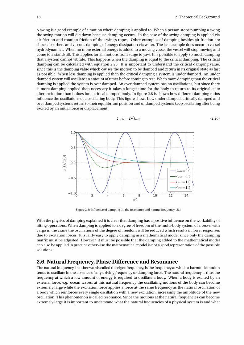
18 2. Theoretical Background
A swing is a good example of a motion where damping is applied to. When a person stops pumping a swingthe swing motion will die down because damping occurs. In the case of the swing damping is applied viaair friction and rotation friction of the swing’s ropes. Other examples of damping besides air friction areshock absorbers and viscous damping of energy dissipation via water. The last example does occur in vesselhydrodynamics. When no more external energy is added to a moving vessel the vessel will stop moving andcome to a standstill. This applies for all motions from surge to yaw. It is possible to apply so much dampingthat a system cannot vibrate. This happens when the damping is equal to the critical damping. The criticaldamping can be calculated with equation 2.20. It is important to understand the critical damping value,since this is the damping value which causes the motion to be damped and return in its original state as fastas possible. When less damping is applied than the critical damping a system is under damped. An underdamped system will oscillate an amount of times before coming to rest. When more damping than the criticaldamping is applied the system is over damped. An over damped system has no oscillations, but since thereis more damping applied than necessary it takes a longer time for the body to return to its original stateafter excitation than it does for a critical damped body. In figure 2.8 is shown how different damping ratiosinfluence the oscillations of a oscillating body. This figure shows how under damped, critically damped andover damped systems return to their equilibrium position and undamped systems keep oscillating after beingexcited by an initial force or displacement.
ξcr i t = 2p
km (2.20)
Figure 2.8: Influence of damping on the resonance and natural frequency [33]
With the physics of damping explained it is clear that damping has a positive influence on the workability oflifting operations. When damping is applied to a degree of freedom of the multi-body system of a vessel withcargo in the crane the oscillations of the degree of freedom will be reduced which results in lower responsesdue to excitation forces. It is fairly easy to apply damping in a mathematical model since only the dampingmatrix must be adjusted. However, it must be possible that the damping added to the mathematical modelcan also be applied in practice otherwise the mathematical model is not a good representation of the possiblesolutions.
2.6. Natural Frequency, Phase Difference and ResonanceThe natural frequency, in other words called the eigenfrequency, is the frequency at which a harmonic motiontends to oscillate in the absence of any driving frequency or damping force. The natural frequency is thus thefrequency at which a low amount of energy is required to oscillate a body. When a body is excited by anexternal force, e.g. ocean waves, at this natural frequency the oscillating motions of the body can becomeextremely large while the excitation force applies a force at the same frequency as the natural oscillation ofa body which reinforces every single oscillation with a new excitation, increasing the amplitude of the newoscillation. This phenomenon is called resonance. Since the motions at the natural frequencies can becomeextremely large it is important to understand what the natural frequencies of a physical system is and what
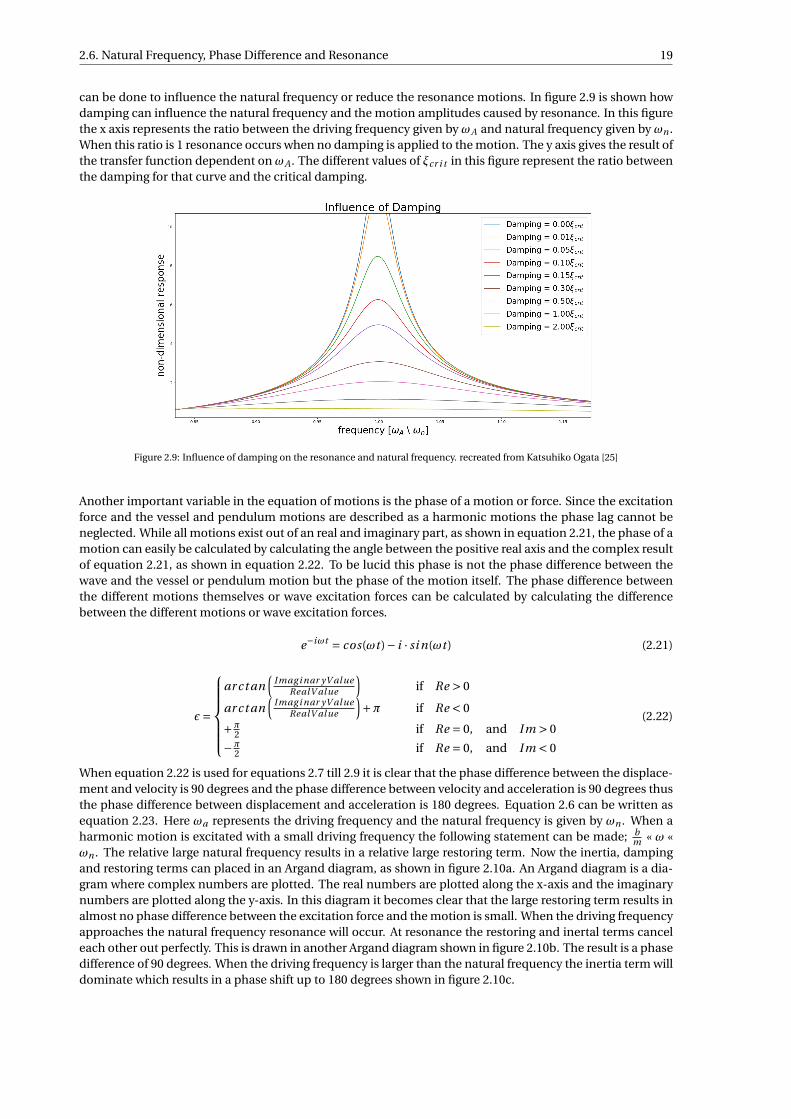
2.6. Natural Frequency, Phase Difference and Resonance 19
can be done to influence the natural frequency or reduce the resonance motions. In figure 2.9 is shown howdamping can influence the natural frequency and the motion amplitudes caused by resonance. In this figurethe x axis represents the ratio between the driving frequency given by ωA and natural frequency given by ωn .When this ratio is 1 resonance occurs when no damping is applied to the motion. The y axis gives the result ofthe transfer function dependent onωA . The different values of ξcr i t in this figure represent the ratio betweenthe damping for that curve and the critical damping.
Figure 2.9: Influence of damping on the resonance and natural frequency. recreated from Katsuhiko Ogata [25]
Another important variable in the equation of motions is the phase of a motion or force. Since the excitationforce and the vessel and pendulum motions are described as a harmonic motions the phase lag cannot beneglected. While all motions exist out of an real and imaginary part, as shown in equation 2.21, the phase of amotion can easily be calculated by calculating the angle between the positive real axis and the complex resultof equation 2.21, as shown in equation 2.22. To be lucid this phase is not the phase difference between thewave and the vessel or pendulum motion but the phase of the motion itself. The phase difference betweenthe different motions themselves or wave excitation forces can be calculated by calculating the differencebetween the different motions or wave excitation forces.
e−iωt = cos(ωt )− i · si n(ωt ) (2.21)
ε=
ar ct an
(Imag i nar yV al ue
RealV al ue
)if Re > 0
ar ct an(
Imag i nar yV al ueRealV al ue
)+π if Re < 0
+π2 if Re = 0, and Im > 0
−π2 if Re = 0, and Im < 0
(2.22)
When equation 2.22 is used for equations 2.7 till 2.9 it is clear that the phase difference between the displace-ment and velocity is 90 degrees and the phase difference between velocity and acceleration is 90 degrees thusthe phase difference between displacement and acceleration is 180 degrees. Equation 2.6 can be written asequation 2.23. Here ωa represents the driving frequency and the natural frequency is given by ωn . When aharmonic motion is excitated with a small driving frequency the following statement can be made; b
m « ω «ωn . The relative large natural frequency results in a relative large restoring term. Now the inertia, dampingand restoring terms can placed in an Argand diagram, as shown in figure 2.10a. An Argand diagram is a dia-gram where complex numbers are plotted. The real numbers are plotted along the x-axis and the imaginarynumbers are plotted along the y-axis. In this diagram it becomes clear that the large restoring term results inalmost no phase difference between the excitation force and the motion is small. When the driving frequencyapproaches the natural frequency resonance will occur. At resonance the restoring and inertal terms canceleach other out perfectly. This is drawn in another Argand diagram shown in figure 2.10b. The result is a phasedifference of 90 degrees. When the driving frequency is larger than the natural frequency the inertia term willdominate which results in a phase shift up to 180 degrees shown in figure 2.10c.

20 2. Theoretical Background
(−ω2a + i ·ωa
B
M+ω2
n)xa e iωt = F0e iωt (2.23)
(a) Argand diagram with largerestoring force [16]
(b) Argand diagram resonancefrequency [16]
(c) Argand diagram with largeinertia term [16]
Figure 2.10: Argand diagrams for different driving frequencies.
The phase difference between an excitation force and corresponding motion can be calculated with equation2.24. In this formula ξ stands for the damping ratio given by b
bcr i t i cal. When the driving frequency ω is small
the equation will give a solution close to 0. When the driving frequency and the natural frequency are equalthe value within the arc-tangent function will be infinite thus the solution for φ0 will be equal to 90 degrees.Finally when the driving frequency is larger than the natural frequency the phase difference will exceed the90 degrees but will never exceed the 180 degrees. The change in phase will influence the interaction betweenthe degree of freedom. When the swing motion of the cargo changes in phase and the roll motion does notchange in phase the two motions will have another interaction and amplitude than when the two motionshave the same phase.
φ0 =0−ar ct an
(ξ 2ωωn
ω2−ω2n
)if ω≤ωn ,
π−ar ct an(ξ 2ωωn
ω2−ω2n
)if ω>ωn
(2.24)
In multi-body dynamics the opposite of resonance can occur. The so called anti-resonance. Anti-resonanceis a pronounced minimum in the amplitude of one oscillator at a particular frequency. When anti-resonanceoccurs there will also be a large shift in the oscillation phase of the body, just as it happens with resonance. It ispossible for multi-body system to reduce the response to almost zero when anti-resonance occurs. However,anti-resonance only reduces the motions of one body to an extreme small response at a time. When anti-resonance occurs all the oscillations of one body are almost reduced to zero by the connection between thetwo different bodies. The motions of the second body will also be small, but it will not be reduced to sucha low minimum as the first body. While resonance can happen at multiple degrees of freedom due to thecoupling.
2.7. Natural Frequencies of Multi-Body SystemsThe formula used to calculate the natural frequency of a single degree of freedom is quite simple. Howeverin multi-body dynamics the equation is a bit harder. All the different degrees of freedom can influence all thenatural frequencies. As a result the natural frequency of a body in a multi-body system can be quite differentthan the natural frequency of a comparable body that is not connected to a multi-body system. In singledegrees of freedom the natural frequency can be calculated with equation 2.25. In this equation K standsfor the stiffness value of the single degree of freedom and M represents the mass of the body. The naturalfrequency calculation of multi-body systems will be explained later in this section. When equation 2.15 andequation 2.25 are combined it is clear that the natural frequency of a single pendulum is equal to equation2.26.
ωn =√
K
M(2.25)

2.7. Natural Frequencies of Multi-Body Systems 21
ωnpendulum =√
g
L(2.26)
A study from MacKay[18] shows that the natural frequencies of of a double pendulum where both pendula
have the same mass and length are equal to 0.8 and 1.8√
gL . This makes it clear that the natural frequency of a
multi-body system can be influenced by different bodies in the multi-body system. Another study regardingsmall oscillations of a n-pendulum model shows that the natural frequencies of multiple degrees of freedompendulum systems is heavily influenced by the amount of pendulums, in other words degrees of freedom.This study is done by Rubenzahl and Rajeev [29]. These studies show that the cargo cannot be seen as a simplependulum and the cargo swing motions must be integrated in a multi-body system to study the influence ofthe vessel and cargo on the natural frequencies of both bodies. Different aspects such as vessel displacement,vessel metacentric height, cargo mass and crane top location do influence the natural frequency of the vesseland cargo motions. Since these values differ per loading operation the natural frequencies will also differper loading operation. Some loading conditions can be varied to change the natural frequency in a desiredway. But before the motions and the natural frequencies can be studied the method to calculate the naturalfrequencies must be calculated.
As explained in section 2.6 the natural frequency the frequency where the influence of the stiffness and mass
is equal to each other. In one degree of freedom motions this is the natural frequency equal to√
CM . In
multiple degree of freedom systems the stiffness and mass values are replaced by matrices. These matricescomplicate the calculations of the natural frequencies but make it possible to calculate the natural frequen-cies of combined motions. In equations 2.27 till 2.31 an example is given for a natural frequency problem of atwo degrees of freedom multi-body system. When the different mass and stiffness values of equation 2.31 areknown the equation can be solved for ωn . Since the resulting natural frequency has to be positive, real anddistinct a maximum of two natural frequencies can occur for a two degrees of freedom system.
det∣∣−ω2
n M x +C x∣∣= 0 (2.27)
∣∣∣∣−ω2n
[M11 M17
M71 M77
][x1
x7
]+
[C11 C17
C71 C77
][x1
x7
]∣∣∣∣= 0 (2.28)
∣∣∣∣([−ω2n
(Mhyd11 + Ahyd11
)0
0 −ω2n
(Mcar g o77
)]+[Chyd11 +Kp −Kp
−Kp Kp
])[x1
x7
]∣∣∣∣= 0 (2.29)
∣∣∣∣[−ω2n
(Mhyd11 + Ahyd11
)+Chyd11 +Kp −Kp
−Kp −ω2n
(Mcar g o77
)+Kp
]∣∣∣∣= 0 (2.30)
ω4n
((Mhyd11 + Ahyd11
)Mcar g o77
)+ω2n
((Mhyd11 + Ahyd11
)Kp +Mcar g o77
(Chyd11 +Kp
))+Chyd11 Kp = 0 (2.31)
In appendix B the mass, damping and stiffness matrices are shown for the 12 degrees of freedom system.The stiffness matrix stands out in density in regards with the mass matrix. This means that there is a lot ofinfluence of the stiffness between different motions and these stiffness factors will influence the natural fre-quencies of the different degrees of freedom. The calculations for the natural frequencies of multiple degreesof freedom systems might be harder but they are not impossible. When the stiffness and mass matrices areknown the natural frequencies can be calculated with the eigenvalue method. Python can be used to calcu-late the natural frequencies with the help of the eigenvalue method. This makes the calculation of naturalfrequencies fairly simple.
Thus different motions can influence each other. As explained in section 2.6 different degrees of freedomhave different phases at certain driving frequencies. This means that two different degrees of freedom thatare coupled at a natural frequency can have a different phase. The difference phases can influence the inter-action between the two degrees of freedom. The different motions can enhance the amplitude of both bodiesbecause both motions move with the same phase in the same direction which reinforces the amplitude orthey move in counter phase of each other which can reduce the excitation amplitude of both motions.

22 2. Theoretical Background
Since the natural frequencies themselves and the calculated responses do not show how the different degreesof freedom influence the different natural frequencies the eigenvectors can be calculated. Eigenvectors showhow the different different degrees of freedom act at the eigenvalues, which are directly linked to the naturalfrequencies. To use the properties of an eigenvector correctly first the definition of an eigenvector must beunderstood.
A vector is an eigenvector when the vector is a non zero vector and the vector does linear transform a matrix bya scalar factor.[9]
In other words an eigenvector of a linear transformation is a non-zero vector that, when applied to this lineartransformation , does not change the direction but only scales the linear transformation by the eigenvalue.The linear transformation could take the form of an n by n matrix. The definition of an eigenvector v is givenin equation 2.33 and in equation 2.34 the definition of a eigenvector of a matrix is given. Equations 2.33 and2.34 show the definition of an eigenvector in their basic forms, however an eigenvector problem can be solvedfor a physical mass-spring system. Equation 2.35 shows how an eigenvalue problem can be used for a mass-spring system. When v is exchanged to x this equation is equal to the equation in the determinant functionof equation 2.27.
λ=ω2n (2.32)
T (v ) =λv (2.33)
Av =λv (2.34)
C v =λM v (2.35)
When the eigenvalues, or natural frequencies, of a multi-body system are known the eigenvectors can be cal-culated. Every single natural frequency in a multi-body system has its own eigenvector. Equation 2.35 canbe written as 2.36. When the mass and spring matrices and the natural frequencies are known this equationcan be used to calculate the eigenvectors. In equations 2.37 till 2.44 an example calculation for eigenvaluesand eigenvectors is given for a double pendulum. In this double pendulum the length and weight of bothpendulum are equal to each other. The first pendulum is connected to the earth fixed coordinate system. Thesecond pendulum is connected to the first weight of the first pendulum as illustrated in figure 2.11. These arethe same values as used in the study done by MacKay[18]. Equations 2.27 till 2.31 showed how complicatedthe natural frequency calculations can become when the stiffness and mass values have complicated rela-tions. The simpler relations from the double pendulum are used to show how the eigenvalue method workswith actual results.
Figure 2.11: Schematic of a double pendulum used in the example calculation of the natural frequencies and eigenvectors [18]
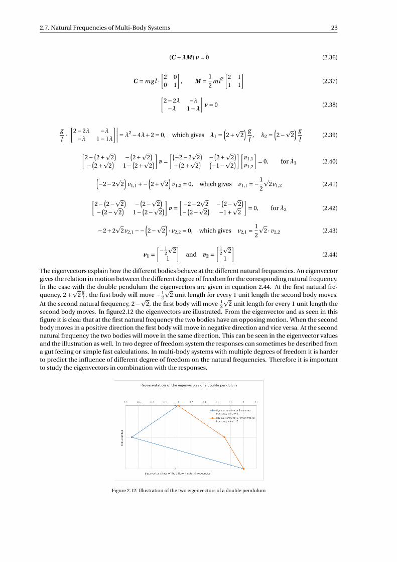
2.7. Natural Frequencies of Multi-Body Systems 23
(C −λM) v = 0 (2.36)
C = mg l ·[
2 00 1
], M = 1
2ml 2
[2 11 1
](2.37)
[2−2λ −λ−λ 1−λ
]v = 0 (2.38)
g
l·∣∣∣∣[2−2λ −λ
−λ 1−1λ
]∣∣∣∣=λ2 −4λ+2 = 0, which gives λ1 =(2+p
2) g
l, λ2 =
(2−p
2) g
l(2.39)
[2− (
2+p2) −(
2+p2)
−(2+p
2)
1− (2+p
2)]v =
[(−2−2p
2) −(
2+p2)
−(2+p
2) (−1−p
2)][
v1,1
v1,2
]= 0, for λ1 (2.40)
(−2−2
p2)
v1,1 +−(2+p
2)
v1,2 = 0, which gives v1,1 =−1
2
p2v1,2 (2.41)
[2− (
2−p2) −(
2−p2)
−(2−p
2)
1− (2−p
2)]v =
[−2+2p
2 −(2−p
2)
−(2−p
2) −1+p
2
]= 0, for λ2 (2.42)
−2+2p
2v2,1 −−(2−p
2)· v2,2 = 0, which gives v2,1 = 1
2
p2 · v2,2 (2.43)
v1 =[− 1
2
p2
1
]and v2 =
[ 12
p2
1
](2.44)
The eigenvectors explain how the different bodies behave at the different natural frequencies. An eigenvectorgives the relation in motion between the different degree of freedom for the corresponding natural frequency.In the case with the double pendulum the eigenvectors are given in equation 2.44. At the first natural fre-quency, 2+p
2 gl , the first body will move − 1
2
p2 unit length for every 1 unit length the second body moves.
At the second natural frequency, 2−p2, the first body will move 1
2
p2 unit length for every 1 unit length the
second body moves. In figure2.12 the eigenvectors are illustrated. From the eigenvector and as seen in thisfigure it is clear that at the first natural frequency the two bodies have an opposing motion. When the secondbody moves in a positive direction the first body will move in negative direction and vice versa. At the secondnatural frequency the two bodies will move in the same direction. This can be seen in the eigenvector valuesand the illustration as well. In two degree of freedom system the responses can sometimes be described froma gut feeling or simple fast calculations. In multi-body systems with multiple degrees of freedom it is harderto predict the influence of different degree of freedom on the natural frequencies. Therefore it is importantto study the eigenvectors in combination with the responses.
Figure 2.12: Illustration of the two eigenvectors of a double pendulum
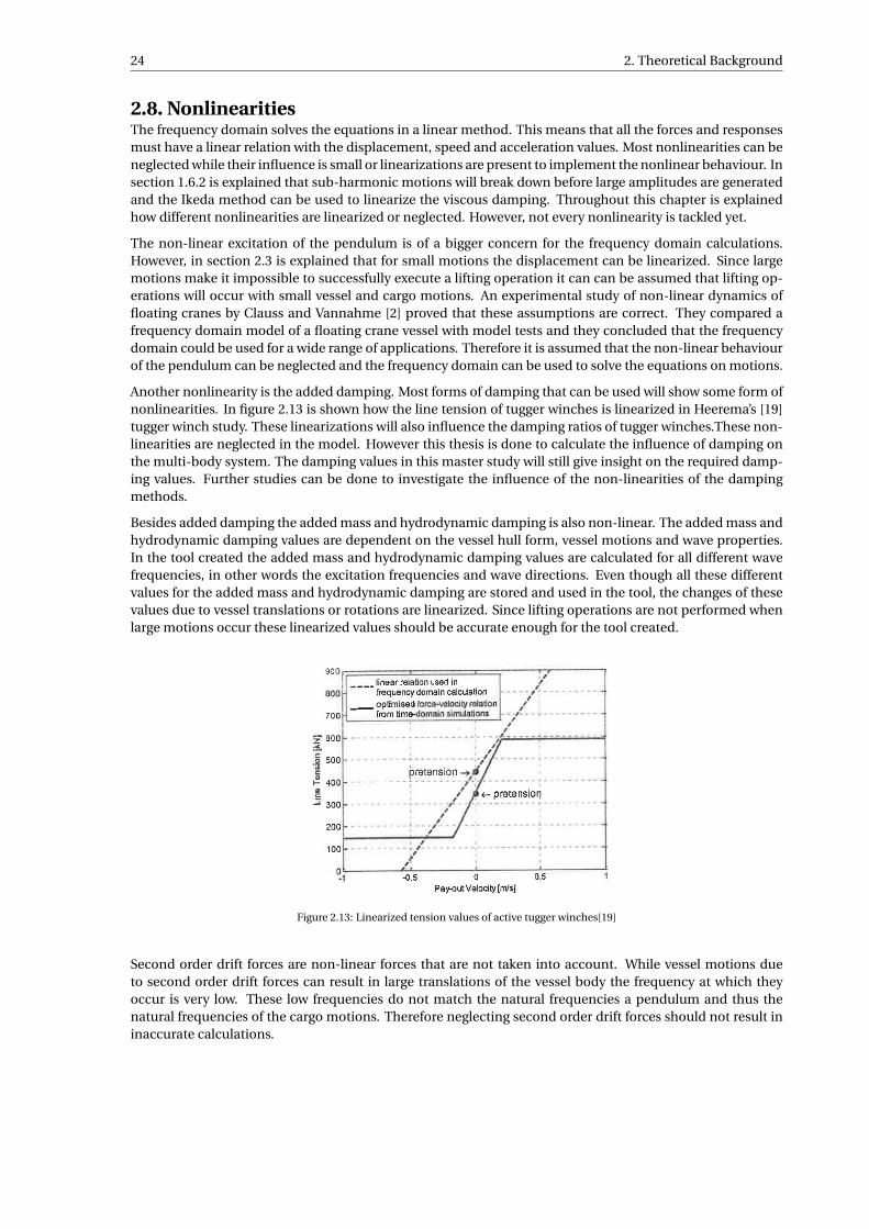
24 2. Theoretical Background
2.8. NonlinearitiesThe frequency domain solves the equations in a linear method. This means that all the forces and responsesmust have a linear relation with the displacement, speed and acceleration values. Most nonlinearities can beneglected while their influence is small or linearizations are present to implement the nonlinear behaviour. Insection 1.6.2 is explained that sub-harmonic motions will break down before large amplitudes are generatedand the Ikeda method can be used to linearize the viscous damping. Throughout this chapter is explainedhow different nonlinearities are linearized or neglected. However, not every nonlinearity is tackled yet.
The non-linear excitation of the pendulum is of a bigger concern for the frequency domain calculations.However, in section 2.3 is explained that for small motions the displacement can be linearized. Since largemotions make it impossible to successfully execute a lifting operation it can can be assumed that lifting op-erations will occur with small vessel and cargo motions. An experimental study of non-linear dynamics offloating cranes by Clauss and Vannahme [2] proved that these assumptions are correct. They compared afrequency domain model of a floating crane vessel with model tests and they concluded that the frequencydomain could be used for a wide range of applications. Therefore it is assumed that the non-linear behaviourof the pendulum can be neglected and the frequency domain can be used to solve the equations on motions.
Another nonlinearity is the added damping. Most forms of damping that can be used will show some form ofnonlinearities. In figure 2.13 is shown how the line tension of tugger winches is linearized in Heerema’s [19]tugger winch study. These linearizations will also influence the damping ratios of tugger winches.These non-linearities are neglected in the model. However this thesis is done to calculate the influence of damping onthe multi-body system. The damping values in this master study will still give insight on the required damp-ing values. Further studies can be done to investigate the influence of the non-linearities of the dampingmethods.
Besides added damping the added mass and hydrodynamic damping is also non-linear. The added mass andhydrodynamic damping values are dependent on the vessel hull form, vessel motions and wave properties.In the tool created the added mass and hydrodynamic damping values are calculated for all different wavefrequencies, in other words the excitation frequencies and wave directions. Even though all these differentvalues for the added mass and hydrodynamic damping are stored and used in the tool, the changes of thesevalues due to vessel translations or rotations are linearized. Since lifting operations are not performed whenlarge motions occur these linearized values should be accurate enough for the tool created.
Figure 2.13: Linearized tension values of active tugger winches[19]
Second order drift forces are non-linear forces that are not taken into account. While vessel motions dueto second order drift forces can result in large translations of the vessel body the frequency at which theyoccur is very low. These low frequencies do not match the natural frequencies a pendulum and thus thenatural frequencies of the cargo motions. Therefore neglecting second order drift forces should not result ininaccurate calculations.

3Model description
In this chapter the model is explained. In section 3.1 the layout of the model is explained. Section 3.2 de-scribes how the vessel hydrodynamics are added to the model. Thereafter the coupling between the cargoand the vessel via the crane cable is explained in section 3.3. Next the modelling of the mooring lines isexplained in section 3.4 followed by the modelling of the cargo control systems in section 3.5. The motioncalculations are explained in section 3.6. In section 3.7 the significant motion calculations are explained. Theverification of the model is worked out in section 3.8 followed by the validation is section 3.9. Lastly, in section3.10, the influence of different parameters of the lifting operation are described. These can be used to alterthe responses of the vessel and cargo during lifting operations.
3.1. Model LayoutFirst of all an overview of the model will be explained. The model is made in the mathematical programminglanguage Python[7]. Python is a language in which multiple different programming modules can be im-ported. These programming modules make it possible to solve different aspects of the mathematical prob-lem. examples are a mathematical tool for mathematical equations, a scientific computing tool for matrixcalculations and a tool to plot results in to graphs. This makes Python a versatile mathematical program.Therefore Python is used to create a tool that can solve the multi-body system. In the Python tool all thedifferent aspects of the multi-body system can be solved via the different programming modules.
In the Python tool created to calculate the responses of the multi-body system, all different mathematicalsystems are implemented separately. This makes the tool modular and different aspects of the lifting opera-tion can be added to the calculation or ignored on purpose. The multi-body tool consists of different pythonsub-files to keep the tool structured. In these sub-files different mathematical steps are fulfilled or matricesare created. There is one main file which is used to summon all different sub files. Besides the main file therewill be a file with all the settings required to solve the mathematical equations. In the settings file all differentsettings for the different sub files are stored. From crane tip position to mooring line configurations and fromvessel hydrodynamics to cargo control system configurations.
In figure 3.1 a schematic drawing of the mathematical model is shown. The first mathematical system that isimplemented in the model are the vessel hydrodynamic properties. The vessel hydrodynamics contain theproperties of the vessel hull and the interaction between the hull and the water. In section 3.2 is explained howthe hydrodynamics are imported. The second part that is implemented is the interaction between the cargobody and the vessel body via the crane. In section 3.3 is explained how the vessel and cargo are connectedvia the crane in a mathematical way. In section 3.4 is explained how the mooring lines are implementedin a mathematical way and which input variables are required to calculate the influence of mooring lines.Cargo control systems can be used to influence the cargo motions during lifting operations. The influenceof cargo control systems are calculated via added stiffness and damping values. Both different influences areimplemented via separate Python sub-files. In section 3.5 is explained how both the stiffness and dampingvalues of the cargo control systems are implemented to the multi-body model. With the cargo control sys-tems implemented all the input values required to translate the mechanical system to a mathematical modelare elaborated. The next part of the model is to solve the mathematical system. In section 3.6 is explainedhow the responses of the mathematical model will be calculated with the help from the different input val-ues. The responses of the multi-body system can be used to calculate statistical maximum responses of themotions. These statistical responses can be used to compare different lifting operations for different liftingconfigurations and different weather conditions. These statistical calculations can be done with the Pythontool and are explained in section 3.7. In section 3.10 is explained how the motions are influenced by differ-ent wave spectra and how different variables of a lifting operation can influence the natural frequency of the
25

26 3. Model description
multi-body system. The verification of the model is explained in section 3.8. In this section different mathe-matical properties of the model are verified. BigLift Shipping has an inhouse lifting simulator which is usedto train onboard crew. This simulator can be used to validate the Python model. The validation is explainedin section 3.9.
Figure 3.1: Schematic drawing off the mathematical model that is created for this study.
3.2. Vessel InputThe vessel input contains all the hydrodynamic properties of the vessel. These properties determine therelation between the hull shape, displacement, center of gravity, center of buoyancy and other properties andincoming waves from all directions. In the paragraph below will be described which hydrodynamic propertiesand how these properties are implemented in this model.
Response Amplitude Operators, RAOs, are transfer functions used to calculate the effect of wave spectra onvessel motions as explained in section 2.2. Many methods and different software is developed to calculateRAOs. Shipmo is such a program that calculates the motion RAOs with the help of 2D linear diffraction the-ory (’strip theory’) [35]. Shipmo is developed by Marin. For this research Shipmo version 17.2.3 is used. In2D strip theory methods the vessel is divided into a finite number of cross sections, or strips. For these stripsthe vessel hydrodynamic properties are calculated. From all these separate hydrodynamic properties the ves-sel’s overall hydrodynamic properties can be calculated. Unfortunately these RAOs themselves are not usefulfor this study since they will only give the transfer function for a vessel without cargo in the crane. HoweverShipmo can also export the mass, added mass, damping, viscous damping and stiffness matrix as well as thecorresponding excitation force vector of the six degrees of freedom of the vessel. These matrices and vec-tor will be used to fill in the first quadrant of the 12 DoF matrices and the first 6 values of the force vector.The mass and hydrodynamic stiffness matrix are constant values for all the weather, vessel heading, vesselspeed and roll amplitude input values. The vessel speed is set to zero in all calculations while lifting opera-tions are mainly performed without forward speed. Thus for different wave frequencies, wave directions androll amplitudes these matrices stay the same. The loading conditions, which contain the displacement andmetacentric height, and hull form do have influence on the mass and hydrodynamic stiffness matrices. How-ever, a shipmo hydrodynamic database can only be created for one specific loading condition and hullform.Therefore a new hydrodynamic database must be created for different loading conditions and hull forms.The added mass and damping are different for various weather and sailing input values. Therefore these ma-trices must be saved for all the different wave directions, wave frequencies roll angles. All the values that areexported from Shipmo are shown in table 3.1.
3.2. Vessel Input 27
The loading conditions of the vessels are a bit tricky. Normally cargo in a crane will be translated to the cranetop for simple stability calculations. However, in this model the cargo dynamics are modelled as an extrabody and therefore the cargo should not be applied to the crane top as a weight. However when the cargo isneglected completely the water displacement is too low because the displacement of the vessel results fromthe vessel and cargo combined mass. Therefore it is assumed that the vessel displacement is the displacementof the vessel weight including the cargo but the stability values are the values of the vessel without the cargo inthe crane. later on in the calculations the weight of the cargo is deducted from the vessel mass matrix. Duringthe hydrodynamics calculation the mass of the cargo is chosen in such a way that it does not influence theloading condition of the vessel other than increasing the draught of the vessel. In practice this means thatthe vessel’s metacentric height will not change between a loading condition without cargo in the crane and aloading condition with cargo in the crane. This property is chosen while the draught increase due to the cargocannot be neglected and the influence of the mass on the vessel motions will be calculated via the multi-bodysystem. On any other location the cargo will have an extra influence on the motions of the vessel.
Shipmo uses hull forms to calculate different aspects of the loading condition. The hull forms of all of BigLiftShipping’s vessels are present in the database to calculate the vessel hydrodynamics with Shipmo. The com-bination of the vessel’s hull form, draught and trim are used to calculate the mass matrix of the vessel body.The hull form is also used to calculate the influence of the hull form on all other hydrodynamic properties.
A problem with 2D linear diffraction theory is that it is not accurate at the determination of roll damping.Significant viscous effects and effects from appendages prevent the strip theory method to create accurateresults. Therefore some empirical formulas and experimental data are used to predict the roll damping in thestrip theory methods. Ikeda et al [13] developed a roll damping prediction method with the same accuracy asstrip theory methods and this method is also based on hydrodynamic forces acting on the cross sections, orstrips, of a vessel. Ikeda’s method can calculate the frictional, wave, eddy and bilge keel aspects of roll damp-ing. A side effect is that Ikeda’s method is not accurate for motion calculations of vessels with a significantforward speed. However this is not a concern for this study because lifting operations are carried out withoutforward speed. Shipmo has a built-in Ikeda method. Therefore the extracted matrices can be used for thePython tool.
Shipmo is a validated and proven tool. Together with the easy access of Shipmo is Shipmo a useful tool for thehydrodynamic aspects of the multi-body tool created for this study. Shipmo is also used by other programssuch as Safetrans. Since Safetrans is used regularly by BigLift Shipping the input files required for Shipmo areup to date and kept up to date for every update of Shipmo. The hydrodynamic coefficients calculations couldalso be carried out manually. However, this would require a lot of time to create a 2D strip theory or 3D panelmethod calculation and programming time. Another option to calculate the vessel hydrodynamics is to createa hydrodynamic database for a few different loading conditions. With these databases and interpolationall required hydrodynamic properties can be calculated. However, this is less accurate than using Shipmoto create hydrodynamic databases. Other programs such as Seaway[11] and Delfrac[3] could also be usedto calculate the hydrodynamic properties of the vessel. However, the last two programs are not as easilyaccessible as Shipmo from BigLift Shipping. While Shipmo is easily accessible and kept up to date at all timesShipmo is chosen as program to calculate the vessel hydrodynamics in this multi-body tool.

28 3. Model description
Table 3.1: Values exported from Shipmo hydrodynamic database
Shipmo export Dependence and Description
Stiffness Matrix The stiffness matrix is dependent on the hull form and the loading condi-tions of the vessel. While a Shipmo hydrodynamic database is made for a spe-cific hull form and a specific loading condition the complete matrix can beexported once for all the different wave frequencies, wave directions, vesselspeeds and roll amplitudes of the vessel.
Mass Matrix The mass matrix is dependent on the hull form and the loading conditionsof the vessel. As explained for the stiffness matrix the mass matrix can be ex-ported from the Shipmo hydrodynamic database file once and this matrix willbe valid for all different wave frequencies, wave directions vessel speeds androll amplitudes the vessel.
Added Mass Matrix The added mass matrix contains the inertia added to the vessel motioncaused by the acceleration of water due to the motions of the vessel. This isdependent on the hull form and loading condition but also dependent onthe motion frequencies and motion direction induced by the wave frequen-cies and wave direction and roll amplitude of the vessel. Therefore the addedmass must be exported for all these specific variables
Damping Matrix The damping matrix contains the hydrodynamic damping caused by the ra-diation of energy due to the displacement of the water around the vessel. Thedamping values are dependent on the hull form and loading condition butthey also depend on motion frequencies and motion direction induced bythe wave frequencies and wave direction. Furthermore the damping ma-trix is also dependend on the roll amplitudes of the vessel. Therefore thedamping values must be exported for all these specific variables. The Ikedamethod[13] is used to calculate the correct roll damping values for the differ-ent appendages.
Wave Excitation Force vec-tor
The wave excitation force vector is a vector which contains the excitationforces for the 6 motions of the vessel body caused by the incoming waves.These forces are dependent on the hull form, loading condition wave fre-quencies, wave directions and vessel speeds. The wave excitation force vectorshould be exported for all these specific variables
Hull Form, Loading con-dition, Wave frequencies,Wave Direction, VesselSpeed, Roll Amplitude
These variables are chosen by the user of Shipmo. The Hull form is specificfor every vessel type. The loading condition contains the vessel draught, trim,GM, CoG and radii of inertia. The wave frequencies, wave directions, ves-sel speeds and roll angles are other variables chosen by the user of Shipmo.While all these variables are chosen by the user the variables are still exportedfrom the hydrodynamic database so that all these values can be checked atany time and the values can be coupled to specific calculations.
All the data in the Shipmo hydrodynamic database are stored in large text files. The Python tool developed tocalculate the vessel and cargo motions scans the data in these text files and exports the hydrodynamic mass,added mass, damping and stiffness matrices as well as the excitation force vector. These matrices and vectorare saved for every variable necessary as explained in table 3.1. For the verification of the model the responseof the six degrees of freedom of the vessel calculated by Shipmo is also exported. The verification is furtherelaborated in section 3.8.
Shipmo can calculate the hydrodynamic properties and wave forces for different frequencies at the once.However, Shipmo has a maximum number of 200 steps in which the wave frequency can vary. This meansthat that the hydrodynamic coefficients and wave excitation force can be calculated for 200 different wavefrequencies. The default settings of Shipmo will calculate the hydrodynamic coefficients and wave excitation
3.3. Crane and Cargo Model 29
force for a range between r ad/s and r ad/s. With 200 steps this results in a stepsize of r ad/s.To reduce this step size smaller ranges are used to calculate the hydrodynamic databases and wave excitationforces with Shipmo. Depending on the graphs that needs to be generated the range and stepsize will beadjusted. Default ranges in this report are r ad/s - r ad/s and r ad/s - ad/s. This resultsin a stepsize of r ad/s and r ad/s respectively. Since the added mass and damping are frequencydependent smaller stepsizes will result in or accurate calculations of the natural frequencies. At the sametime the graphs created and shown in this report will have a higher resolution.
3.3. Crane and Cargo ModelIn this model the multibody system is excited by the waves. Wind forces will not applied. It is assumed thatthe wind force is relatively small and constant during lifting operations. Due to the relatively small forces thewind will barely influence the cargo motions. When high wind forces occur it is unsafe to execute a liftingoperation hence high wind forces will not occur during actual operations. In a frequency domain calculationconstant forces will not influence the amplitude of the motion. A constant force will result in a standarddisplacement of the equilibrium. For example a constant wind force in longitudinal direction can displacethe cargo by one meter in surge direction. Since the force is constant the new location of the cargo will bethe new equilibrium and the constant wind forces will not introduce any motions in the system. However, itis unlikely for a wind gust to have harmonic behaviour. Without this harmonic behaviour the superpositionprinciple explained in section 2.2 cannot be applied. Due to the small influence on the amplitude of themotions and the non-harmonic behaviour the implementation of wind forces are neglected. This does alsomean that only the body of the vessel gets directly excited by external forces and that the cargo will only movedue to the connection to the vessel motions. When no tugger wires or other damping devices are used, thecrane wire is the only connection between the vessel and the cargo in the crane. In section 2.3 is describedhow the pendulum forces result from the restoring stiffness and how the wire can be described as a, very stiff,spring for motions in the vertical direction.
Now that these stiffness components are described it is time to describe the conditions of the connectionbetween the vessel and cargo. The vessel and the cargo are connected via the crane cable. The crane cableruns from the crane winch to the hook. However, there is a stationary sheave at the crane top. This stationarysheave prohibit motions in the cable between the cable winch and the sheave. Therefore it is assumed thatthe connection between the vessel and the crane cable is located at the stationary sheave at the crane top.The crane hook is connected to the cargo. This connection can be a direct connection, a connection viamultiple slings or a connection via a lifting beam. When the hook is directly connected to the cargo it canbe reasoned that both the body of the hook and the body of the cargo can be modelled as one bodies. Thedistance between the two centres of gravity is small and the weight of the cargo is often a lot higher than theweight of the crane hook. In these situations the crane hook body can be neglected. When the crane hook isconnected via slings to the cargo there will be a significant distance between the cargo and the crane hookand between the crane hook and the crane tip. The hook can be seen as an extra body. Since the weight of thecrane hook is relatively light in comparison with the cargo and the weight of the crane cables and slings theinfluence of such an extra body will be minimal. Therefore the influence of the crane hook will be neglected.The usage of a lifting beam requires the implementation of another extra body to the multibody system. Alifting beam will be relatively light which results in a small influence on the motions. At the same time not alllifting operations are done with the help of lifting beams. Therefore it is assumed that lifting beams are notused in this research. Another aspect that must be considered is the rotation of the cargo. For small and largerotations of the cargo different influences can be considered. One of the considerations is a mechanism thatconsists out of a rotational spring attached in the centre of gravity of the cargo. This mechanism is illustratedin figure 3.2a. In this mechanism it is assumed that the cargo rotates around the centre of gravity of thecargo and that the rotational force is compensated by the spring stiffness of the grommets or slings whichconnect the crane hook to the cargo. In other words the rotation of the cargo will not influence the cranecable. A second mechanism, shown in figure 3.2b, takes the influence of cargo rotations on the crane cableinto account. In this mechanism the crane hook and cargo can be modelled as a double pendulum. Whena double pendulum is considered the rotations of the cargo will create a horizontal translation of the cranehook. However, the radii of inertia of the cargo is much larger than the radii of inertia of the crane hookthe influence of cargo rotations will be small. At the same time will large rotations create an unsafe workenvironment and lifting operations will not be executed in unsafe environments. Due to the small influenceof the second mechanism and the requirement of a safe working environment the first mechanism will be

30 3. Model description
used. The crane cable will be modelled as a wire and not as a rigid connection. This means that the rotationsof the cargo will not influence the crane cable. At the same time it simplifies the calculations since no extrabody needs to be introduced to create a double pendulum model.
The stiffness values of the lifting configuration can differ per type of configuration. In equation 2.17 is ex-plained how the stiffness values of the crane wire can be calculated. The crane cable has a modulus of elastic-ity equal to 110 kN /mm2 and the diameter of the crane cable is equal to 50 mm. Depending on the requiredlifting capacity the amounts of revolutions of the crane cable between the crane winch and crane hook canvary. A common amount of revolutions is 16. When the distance between the crane tip and crane hook isequal to 20 meters the crane wires have a stiffness value of 173.000 kN /m. The same equation can be used tocalculate the stiffness values of the grommets. Depending on the grommets used the elasticity, length of thegrommet and grommet diameter and thus cross sectional area does change. Therefore the stiffness values ofevery type of grommet does change. According to LLoyd’s Register Rules and Regulations - Rules and Regula-tions for the Classification of Ships par 3 Ship Structures (General) - Chapter 14 Cargo Securing Arrangements- Section 9 Strength of container securing arrangements[17] the effective modulus of elasticity for steel wirerope is equal to 90 kN /mm2. Grommets with a working load limit of 100 mton and a nominal length of 4meters have a diameter of 84 mm. This results of a stiffness of 124.000 kN /m per grommet used in the config-uration. Grommets with a working load limit of 150 mton and a nominal length of 10 meters have a diameterof 102mm. This results in a stiffness of 73.500 kN /m. Since the lifting configuration will never consist out of asingle grommet but multiple grommets connected to the hook the stiffness of the grommet configuration willincrease. Since the stiffness of the grommets have the same magnitude as the crane cable wire the stiffness ofthe grommets will not be implemented in the multi-body system. For simplicity is assumed that the stiffnessof the grommet configuration is equal to the stiffness of the crane cable. In the model the crane cable lengthwill be equal to the distance between the crane tip and the centre of gravity of the cargo.
(a) Mechanism for small cargo rotations [10](b) Mechanism for bigger cargo
rotations [10]
Figure 3.2: Representation of the influence of small and large rotations of the cargo on the crane cable configuration
The conditions set for the connection between the vessel and cargo via the crane cable make it possible towrite down mathematical equations for this connection. First of all the cargo will be modelled as a pendulumconnected to the vessel. The pendulum behaviour is explained in section 2.3. It is assumed that the top part ofthe crane cable is connected to the crane tip and the bottom part of the pendulum is connected to the centreof gravity of the cargo. When a relative translation occurs between the crane top and centre of gravity of thecargo in one of the two horizontal directions the restoring stiffness, explained in equation 2.15, together withthe relative translation will cause a restoring force. A relative vertical translation between the crane tip andcentre of gravity of the cargo will result in a restoring force caused by the stiffness of the crane wire, explainedin equation 2.17. It is pretty clear that a translation of one of the two bodies in the multi-body system willcause a translation of the crane tip or a translation of the centre of gravity of the cargo. However, since thecrane tip is a fixed point with respect to the vessel centre of gravity the rotations of the vessel will also cause atranslation of the crane tip. For example, when the roll motion is multiplied with the vertical location of thecrane tip a translation in the sway direction occurs. Even though the rotations might be small the long armscan cause a significant motion. Therefore the influences of the vessel rotations cannot be neglected. At thesame time will the translations of the crane tip and cargo create rotation moments due to the same relationthe rotations have on the translation of the crane tip. When the crane tip or cargo undergoes a translation arestoring force will occur. This restoring force multiplied by the lever arm will cause a rotational moment. In

3.3. Crane and Cargo Model 31
equation 3.1 is shown how the vessel surge, pitch and yaw and the cargo surge motion influence the restoringforce in the vessel surge motion. Equation 3.2 shows the influence of the different degree of freedom on thevessel roll restoring stiffness. All the different influences of the translations and rotations can be coupled inthe restoring stiffness matrix. Via the superposition principle this restoring stiffness matrix can be added tothe equation of motions. In table 3.2 is described which variables are used to create the restoring stiffnessmatrix. In appendix A the free body diagrams are shown. In these figures can be seen how the restoring forcesfollow from displacements in all directions. The free body diagrams of the vessel surge and vessel roll motionare also shown in figure 3.3.
In figure 3.3a can be seen that the surge motion causes a translation of the vessel. Due to this translation thereis an offset between the crane tip and the centre of gravity of the cargo. When there is a offset in longitudinaldirection between the crane tip and the cargo centre of gravity a restoring force in surge direction is created. 4different degrees of freedom can cause an offset between the crane tip and the cargo centre of gravity. Whichresults in a restoring force in longitudinal direction. These degrees of freedom are are summarized below.In equation 3.1 the equation of the restoring force applied to the multi-body system via the crane cable isshown.
• Vessel surge: The vessel surge motion translates the crane tip in longitudinal direction.
• Vessel pitch: The vessel pitch motion multiplied with the vertical location of the crane tip causes atranslation of the crane tip in the longitudinal direction.
• Vessel yaw: The vessel yaw motion multiplied with the transverse location of the crane tip causes atranslation of the crane tip in the longitudinal direction.
• Cargo surge: The cargo surge motion translates the centre of gravity of the cargo in longitudinal direc-tion.
In figure 3.3b the free body diagram of the vessel roll motion is given. A moment in the vessel roll directionis created by a force in the Y or Z direction miltiplied with an arom of theat force to the X-axis. In equation3.2 the pendulum restoring forces acting in the vessel’s roll direction are shown. In total 7 degrees of freedomhave an influence on the vessel roll moment via the pendulum restoring forces. These degrees of freedom aresummarized below.
• Vessel sway: The vessel sway motion will cause a translation of the crane tip. Together with the restor-ing stiffness a restoring force is created. This restoring force will cause a moment in roll direction whenthe force is multiplied with the vertical location of the crane tip.
• Vessel heave: The vessel heave motion will cause a translation of the crane tip. Together with therestoring stiffness a restoring force is created. This restoring force will cause a moment in roll directionwhen the force is multiplied with the transverse location of the crane tip.
• Vessel Roll: The vessel roll motion can cause a moment force in two ways.
∗ The vessel roll motion together with the vertical location of the crane tip creates a translation ofthe crane tip in Y direction. This translation multiplied with the Y component of the restoring stiff-ness creates a force. This force creates a moment when it is multiplied with the vertical locationof the crane tip.
∗ The vessel roll motion together with the transverse location of the crane tip creates a translationof the winch in Z direction. This translation multiplied with the Z component of the restoringstiffness creates a force. This force creates a moment when it is multiplied with the transverselocation of the crane tip.
• Vessel pitch: The vessel pitch motion together with the longitudinal location of the crane tip createsa translation of the crane tip in Z direction. This translation multiplied with the Z component of therestoring stiffness creates a force. This force creates a moment when it is multiplied with the transverselocation of the crane tip.

32 3. Model description
• Vessel yaw: The vessel yaw motion together with the longitudinal location of the crane tip creates atranslation of the crane tip in Y direction. This translation multiplied with the Y component of therestoring stiffness creates a force. This force creates a moment when it is multiplied with the verticallocation of the crane tip.
• Cargo sway: The cargo sway motion will cause a translation of the centre of gravity of the cargo. To-gether with the restoring stiffness a restoring force is created. This restoring force will cause a momentwhen this force is multiplied with the vertical location of the crane tip.
• Cargo heave: The cargo heave motion will cause a translation of the centre of gravity of the cargo. To-gether with the restoring stiffness a restoring force is created. This restoring force will cause a momentwhen this force is multiplied with the transverse location of the crane tip.
In appendix C the complete equation of motions are given. In these equations of motions the influence of thependulum restoring stiffness on all degrees of freedom can be found.
(a) Free body diagram of the interaction between the vesseland cargo via the crane cable for the surge motion of the
vessel
(b) Free body diagram of the interaction between the vesseland cargo via the crane cable for the vessel roll motion
Figure 3.3: Free body diagram of the interaction between the vessel and cargo via the crane cable for the vessel surge motion and thevessel roll motion. These free body diagrams can be used to explain the influence of these degree of freedom on other degrees of
freedom in the multi-body system
Fr es1 = Kp · x1 +Kp ·ZCr ane · x5 −Kp ·YCr ane · x6 −Kp · x7 (3.1)
Fr es4 =−Kp ·ZCr ane · x2 +Kw ·YCr ane · x3 +Kp ·ZCr ane ·ZCr ane · x4 +Kw ·YCr ane ·YCr ane · x4
−Kw ·XCr ane ·YCr ane · x5 −Kp ·XCr ane ·ZCr ane · x6 +Kp ·ZCr ane · x8 −Kw ·YCr ane · x9(3.2)

3.3. Crane and Cargo Model 33
Equations 3.1 and 3.2 show how the restoring forces of the pendulum can be calculated. However, theseequations do not show how the restoring stiffness matrices are created in the Python tool. In equation 3.3is showed how the restoring stiffness values of equation 3.1 are written in a matrix. Equation 3.4 shows howthe stiffness values of equation 3.2 can be written in a matrix. When this is done for all degrees of freedomthe pendulum stiffness matrix is created. In section 3.6 is explained how this matrix is implemented in themulti-body system.
Cpendul um11 = Kp
Cpendul um15 = Kp ·Zcr ane
Cpendul um11 =−Kp ·Ycr ane
Cpendul um17 =−Kp
(3.3)
Cpendul um42 =−Kp ·Zcr ane
Cpendul um43 = Kw ·Ycr ane
Cpendul um44 = Kp ·Zcr ane ·Zcr ane +Kw ·Ycr ane ·Ycr ane
Cpendulum45 =−Kw ·Xcr ane ·Ycr ane
Cpendul um46 =−Kp ·Xcr ane ·Zcr ane
Cpendulum48 = Kp ·Zcr ane
Cpendulum49 =−Kw ·Ycr ane
(3.4)
The Python tool uses the input values explained in table 3.2 to calculate the pendulum restoring stiffnessvalues. With this restoring stiffness value and the location of the crane top and the length of the crane cablethe stiffness values for all 12 degrees of freedom can be calculated. A 12 by 12 matrix is created and filled withall the pendulum stiffness values. In section 3.6 is explained how this matrix is used to calculate the responsesof the multi-body system.
Table 3.2: Input values needed to calculate pendulum stiffness matrix
Input Used for
Cargo Mass Used to calculate pendulum stiffness and to calculate the critical damping.
Sling length The sling length contains the vertical distance between the crane tip andcargo CoG sed to calculate pendulum stiffness and the wire stiffness. In themodel the term sling length is used but in practice it is the combined lengthof the crane cable, crane hook and slings. The sling length is used to calculatethe influence of the vessel rotations on the pendulum motions.
Young’s modulus cranewire
Used to calculate wire stiffness.
Crane wire cross sectionalarea
Used to calculate wire stiffness.
Difference between vesseland cargo CoG
Used to translate the rotations of the vessel in translations of the crane tipand used to translate cargo translations in rotational moments. Both are usedto calculate the influence of the 12 DoF on each other.
A variable that must not be forgotten is air friction. Air friction causes damping to the pendulum motionsbut this is a damper that only acts on the pendulum and will not act as a damper between the two motions.While the air damping is very small it is assumed that the air damping is 0.5% of the critical damping[14]. Toimplement the air damping a matrix is created which contains the air damping values.

34 3. Model description
3.4. Mooring Lines Input
Mooring lines will add stiffness to the system. Since mooring lines are only connected to the vessel they willonly add stiffness to the vessel. However, since it is a multi-body system the stiffness connected to the vesselbody will also influence the cargo responses. Therefore the influence of mooring lines are studied. The resultsof this study are shown in section 5.2. The weight of the mooring lines will be neglected. Even though the sizeof the mooring lines can become large in both length and diameter, the weight of the lines will always be smallin comparison with the vessel and cargo. The vessel could lift cargoes with less weight but this study does notfocus on light weight cargo. Due to the relatively small mooring line weights the weight will not influence themass of the vessel at all. Without weight the mooring lines will only influence the stiffness components of themulti-body system. The stiffness values will cause restoring forces when the vessel displaces from its originalposition. These restoring forces will counteract the inertia forces. While the inertia terms will not change anew balance between the restoring forces and inertia forces will be found when mooring lines are added tothe system. The natural frequencies of the multi-body system are dependent on the stiffness and mass of themulti-body system as explained in section 2.7. The increased stiffness due to the mooring lines will increasethe natural frequencies of the multi-body system.
The mooring lines will be described as springs. The spring stiffness of the mooring lines can be linearizedfrom the elongation graph as explained in section 2.4. Besides the breaking load of a mooring line the lengthof the mooring line is required to calculate the spring stiffness. To calculate the overall length the X, Y andZ locations of the bollards on shore and the fairlead of the mooring winch relative to the vessel CoG areneeded. With these values the difference in the X, Y and Z location of each line can be calculated. The overallline length can be calculated with equation 3.5. This line length can be used to calculate the stiffness of themooring line.
In figure 3.4 the linearization graph shown in section 2.4 is shown for clarity. This figure can be used to cal-culate the stiffness values of the mooring lines. When the polypropylene mooring line is linearized for a loadequal to 0 % till 10% of the minimum breaking load an elongation of 1.75% will occur. The total elongationis 1.75% of the line length calculated in equation 3.5. This stiffness can be used to calculate the X, Y and Zstiffness components of the mooring line as shown in equation 3.6. In these equations Kmoor represents thestiffness component of the mooring lines. Xbol l ar d , Ybol l ar d and Zbol l ar d represent the X,Y and Z coordinateof the coordinate on shore relative to the vessel’s centre of gravity. The X,Y and Z coordinate of the winch orfairlead of the mooring line are given by Xwi nch , Ywi nch and Zwi nch respectively.
Ll i ne =√
(Xbol l ar d −Xwi nch)2 + (Ybol l ar d −Ywi nch)2 + (Zbol l ar d −Zwi nch)2 (3.5)
Kmoorx = Kmoor · Xbol l ar d −Xwi nch
Ll i ne
Kmoory = Kmoor · Ybol l ar d −Ywi nch
Ll i ne
Kmoorz = Kmoor · Zbol l ar d −Zwi nch
Ll i ne
(3.6)

3.4. Mooring Lines Input 35
Figure 3.4: Load elongation curves of different mooring line materials[6]
Now that the stiffness components of a single mooring line are known the influence of the lines of the equa-tion of motion can be determined. The values of Kmoorx , Kmoory and Kmoorz can be multiplied with thetranslations to get a force. When the rotations of the vessel are multiplied with the X, Y or Z component ofthe fairlead location a translation of the fairlead is the result. This can be multiplied with the correspondingKmoorx , Kmoory or Kmoorz to get coupling forces between translations and rotations. At the same time, whentranslations are multiplied with the X, Y or Z components of the fairlead location rotational forces will be theresult. Which couples the rotations and translations.
In figure 3.5a the free body diagram of the interaction between the vessel and the shore via the mooringlines for the vessel surge motion is shown. The translation of the surge motions causes an offset between thefairleads and the bollards. This offsets causes the mooring lines to stretch which results in a restoring force inthe mooring lines that is applied to the vessel and the bollard. The shore itself is not part of the multi-bodysystem and the bollards are assumed rigid. Therefore the bollards are unable to move and no new degrees offreedom are introduced. This means that the restoring forces of the mooring lines will only be applied to thevessel body. 3 different degrees of freedom can cause a translation in X direction of the vessel’s fairlead. Thesedegrees of freedom are summarized below. All these degrees of freedom cause a restoring force in the vessel’ssurge direction that is equal to the X component of the mooring line stiffness multiplied by the translation ofthe fairlead in X direction, as shown in equation 3.7.
• Vessel surge: The vessel surge motion translates the fairlead in longitudinal direction.
• Vessel pitch: The vessel pitch motion multiplied with the vertical location of the fairlead causes a trans-lation of the fairlead in the longitudinal direction.
• Vessel yaw: The vessel yaw motion multiplied with the transverse location of the fairlead causes a trans-lation of the fairlead in the longitudinal direction.
Figure 3.5b shows the free body diagram of the interaction between the vessel and the shore via the mooringlines for the vessel roll motion. When the fairleads are not located at the centre of gravity of the vessel fivedifferent degrees of freedom can apply rotational moments in the vessel’s roll direction, as shown in equation3.8. All the degrees of freedom that can influence the vessel roll motion will are summarized below.
• Vessel sway: The vessel sway motion will cause a translation of the fairlead. Together with the restoringstiffness a restoring force is created. This restoring force will cause a moment in roll direction when theforce is multiplied with the vertical location of the fairlead.

36 3. Model description
• Vessel heave: The vessel heave motion will cause a translation of the fairlead. Together with the restor-ing stiffness a restoring force is created. This restoring force will cause a moment in roll direction whenthe force is multiplied with the transverse location of the fairlead.
• Vessel Roll: The vessel roll motion can cause a moment force in two ways.
∗ The vessel roll motion together with the vertical location of the fairlead creates a translation of thefairlead in Y direction. This translation multiplied with the Y component of the restoring stiffnesscreates a force. This force creates a moment when it is multiplied with the vertical location of thefairlead.
∗ The vessel roll motion together with the transverse location of the fairlead creates a translationof the winch in Z direction. This translation multiplied with the Z component of the restoringstiffness creates a force. This force creates a moment when it is multiplied with the transverselocation of the fairlead.
• Vessel pitch: The vessel pitch motion together with the longitudinal location of the fairlead createsa translation of the fairlead in Z direction. This translation multiplied with the Z component of therestoring stiffness creates a force. This force creates a moment when it is multiplied with the transverselocation of the fairlead.
• Vessel yaw: The vessel yaw motion together with the longitudinal location of the fairlead creates atranslation of the fairlead in Y direction. This translation multiplied with the Y component of the restor-ing stiffness creates a force. This force creates a moment when it is multiplied with the vertical locationof the fairlead.
Equations 3.7 and 3.8 are the restoring stiffness calculations for a single mooring line. This equation canneeds to be solved for every mooring line in the multi-body system. Since linear theory is applied the super-position rule can also be used for the mooring lines. All the individual mooring line restoring forces can beadded together to get the total mooring line restoring force.
(a) Free body diagram of the interaction between the vesseland the shore via the mooring lines for the surge motion of
the vessel
(b) Free body diagram of the interaction between the vesseland the shore via the mooring lines for the vessel roll
motion
Figure 3.5: Free body diagram of the interaction between the vessel and the shore via the mooring lines for the vessel surge motion andthe vessel roll motion. These free body diagrams can be used to explain the influence of these degree of freedom on other degrees of
freedom in the multi-body system

3.4. Mooring Lines Input 37
FMoor1 = Kmoorx · x1 +KmoorX ·Zwi nch · x5 −KmoorX ·Ywi nch · x6 (3.7)
FMoor4 =−Kmoory ·Zwi nch · x2 +Kmoorz ·Ywi nch · x3
+KmoorZ ·Ywi nch ·Ywi nch · x4 +Kmoory ·Zwi nch ·Zwi nch · x4
−Kmoorz ·Xwi nch ·Ywi nch · x5 −Kmoory ·Xwi nch ·Zwi nch · x6
(3.8)
Equations 3.7 and 3.8 show how the forces due to one single mooring line can be calculated. The stiffnessvalues components of these equations can be written in a matrix. Equations 3.9 and 3.10 show how themooring stiffness components of a single mooring line can be written in a matrix. For every single mooringline in a lifting configuration such a matrix has to be created. Since the model is a linear model the differentmooring line stiffness matrices can be added together which results in a overall mooring line stiffness matrix.In section 3.6 is explained how this overall stiffness matrix is implemented in the multi-body system. All theinput variables required to solve the mooring line restoring matrix are shown in table 3.3
Cmoor11 = Kmoorx
Cmoor15 = Kmoorx ·Zwi nch
Cmoor16 =−Kmoorx ·Ywi nch
(3.9)
Cmoor12 =−Kmoory ·Zwi nch
Cmoor13 = Kmoorz ·Ywi nch
Cmoor14 = Kmoorz ·Ywi nch ·Ywi nch +Kmoory ·Zwi nch ·Zwi nch
Cmoor15 =−Kmoorz ·Xwi nch ·Ywi nch
Cmoor16 =−Kmoory ·Xwi nch ·Zwi nch
(3.10)
Fenders are neglected in the model. While the influence of the quay is neglected fenders will also be ne-glected. Fenders are also extremely non-linear. Implementing and linearizing fenders would cause largedeviations from reality. When fenders are linearized they will also apply stiffness to the system when the ves-sel moves away from the quay. While fenders have a large stiffness value this would create large restoringforces due to the fenders while they do not occur in reality.
In this method a few assumptions are made. First of all the mooring line stiffness is linearized. This will givea small deviation to reality but is not really important. More important is the fact that considering mooringlines to act linear is only partly true. When elongation occurs the mooring line acts as a spring. Howeverno suspension occurs in a mooring line system. The mooring line will simply go slack and thus no energyis stored in a spring. Assumed that a vessel is moored alongside a quay the problem of slack mooring linescan be solved by placing the mooring lines in forward as backward direction from the vessel so that Kmoorx isthe same in positive as negative direction. In Y direction the mooring line stiffness will only be applied whenthe vessel motion is in the opposite direction than the location of the quay. This will give a false assumptionfor motions towards the quay. However fenders between the vessel and the quay will have a much higherstiffness and this fact can be neglected. Assumed that the fairlead Z position is higher than the bollard Zposition the stiffness of the mooring line will only have influence on a positive heave motion. This is aninaccuracy that must be accepted for practicality when the mooring line stiffness is applied in the frequencydomain. To neglect the stiffness in Z direction the fairlead and bollard position must have the same value fortheir Z position.

38 3. Model description
Table 3.3: Input values needed to calculate the mooring line stiffness matrix
Input Used for
bollard X, Y and Z position 3 lists with the same length. Each input value corresponds to a single bollardon the shore. The values are used to calculate the X, Y and Z distance betweenthe bollards on the quay and the location of the fairlead used by the corre-sponding mooring line.
Fairlead X, Y and Z posi-tion
3 lists with the same length. Each input value corresponds to a single fairleadon board of the vessel. The values are used to calculate the X, Y and Z distancebetween the fairlead and the corresponding bollard on the quay.
MBL mooring line The minimum breaking load is used to calculate the mooring line stiffness asexplained in equation 2.18.
Elongation mooring line The elongation caused by a certain amount of load in % of the total mooringline length. This is used to calculate the the mooring line stiffness.
In the Python tool a new 12 by 12 matrix is created. The input values from table 3.3 can be used to calculatethe stiffness forces of the mooring lines on all degrees of freedom. These stiffness values for all degrees offreedom will be stored in the newly created mooring stiffness matrix. This matrix can be used to calculate theinfluence of mooring lines on the responses of the multi-body system. In section 3.6 will be explained howthe mooring line matrix can be used.
While this matrix has the same dimensions as all other matrices in the mathematical multi-body model, inreality only the upper left quadrant of the matrix will be filled and the other quadrants will only contain zeroentries. While the mooring lines are only a connection between the vessel and the shore there is no couplingbetween the mooring lines and the cargo. This does not mean that the mooring lines will not influence theresponses of the cargo. While the vessel will be influenced by the mooring lines and the cargo is coupled tothe vessel the cargo will also be influenced by the mooring lines.
3.5. Cargo Control SystemsBesides influencing the motions by changing the loading conditions damping can be added to the system toreduce the responses of the vessel and cargo. In section 2.5 is explained what the influence of damping is onthe dynamics of a single or multi degree of freedom system. Damping will dissipate energy from the systemsince the damping forces act perpendicular on the restoring forces and inertia forces, as explained in section2.6. In the same section different methods to apply damping are explained. Passive damping can be appliedvia a system that is related to passive heave compensation systems. Active system can also be used. Constanttension winches and active winches will apply damping to the system.
All the different damping methods have one thing in common. There need to be a connection between thevessel and cargo other than the connection via the crane cable. This connection can be made via tuggerwires. These tugger wires can be connected to the cargo via padeyes or other connection methods. The otherend of the wires can be connected to winches on deck. The tugger winches can pretension the tugger wiresto prevent these wires from falling slack which induces snap loads. Since snap loads can create dangerousforces they need to be prevented. At the same time snaploads are non-linear which makes it impossible toimplement. The stiffness of the tugger winches varies for different materials and different pretension values.In section 2.4 is explained how lines can be linearized. Since pretension is required in the tugger lines thestiffness will not be linearized around the 0% and 10%. The pretension will induce elongation of the line.Depending on the maximum breaking load of the line, the materials, tugger wire length and the pretensionthe tugger wires will be linearized around an appropriate elongation percentage.
The length of the tugger wires can be calculated in an almost identical way as the length of the mooring linesexplained in section 3.4. In the model the location of the tugger winches and the location of the padeyes orother connection methods to the cargo are variables that can be used. The location of the tugger winch is thelocation relative to the vessel centre of gravity. The location of the padeye is the location relative to the centreof gravity of the cargo. Therefore the centre of gravity of the cargo relative to the vessel centre of gravity must

3.5. Cargo Control Systems 39
be taken into account. The centre of gravity of the cargo is dependent on the crane tip location and verticaldistance between crane tip and cargo centre of gravity. In equations 3.11 till 3.13 the equations for the tuggerwire components are given. Equation 3.5 can be used to calculate the total tugger wire length. The stiffnesscomponents of the different directions can be calculated in the same was as the stiffness components of themooring lines. In these equations X tug , Ytug and Ztug represent the X, Y and Z coordinates of the tuggerwinches relative to the vessel’s centre of gravity. The X, Y and Z coordinate of the connection of the tuggerwire to the cargo relative to the cargo’s centre of gravity is given by Xpad , Ypad and Zpad respectively. Thedistance between the crane top and the cargo’s centre of gravity is given by Zsl i ng .
LtugX =√(
XTug −(Xcr ane +Xpad
))2 (3.11)
LtugY =√(
YTug −(Ycr ane +Ypad
))2 (3.12)
LtugZ =√(
ZTug −((
Zcr ane −Zsl i ng)+Zpad
))2 (3.13)
The tugger wires can be made of different materials. All the different materials will have other stiffness values.These stiffness values will influence the multi-body system. To determine the influence of the stiffness of thetugger lines different stiffness values will be compared. In section 6.1 different stiffness values are compared.In this comparison no damping is applied and only the stiffness values will influence the responses of thevessel and cargo.
One of the ways to implement damping to the system was the use of a passive system that dissipates energyvia a hydraulic or pneamatic module. Dissipation forces transfer kinetic energy from the vessel and cargointo heat and kinematic energy of the fluid. Such a system can be connected between the cargo and thevessel with the help of a tugger winch. Both sides of the passive damping module will be connected to twodifferent wires. One wire will be connected to the cargo and the other wire will be connected to the winch.The pretension of the winch can be used to apply the required force to the module and prevent the wiresfrom falling slack. When there is a relative motion between the vessel and cargo the piston of the passivecompensation will extend or contract. As explained in section 2.5 and appendix E, it is hard to determine thedamping of such a system. However damping is possible. Since it is not the purpose of this thesis to develop apassive damping system the exact amount of damping that can be added to the multi-body system will not becalculated. Therefore the damping induced will be taken as a percentage of the critical damping. The critcaldamping used in these calculations is depending on the stiffness of the connection between the cargo andvessel as shown in equation 3.14. In this equation Mcar g o represents the cargo mass and CTug g er representsthe combined stiffness of the tugger wire and damping module.
ξcr i tTug = 2 ·√
Mcar g o ·CTug g er (3.14)
Another way to apply damping is via constant tension winches. Constant tension winches apply dampingdue to the slow activation of the system. As it was for the passive damping module it is hard to determinethe damping of such a system. Therefore the same principle will be used and an percentage of the criticaldamping will be as damping of the system.
The damping that is applied via both ways is the total damping that will be applied. This means that it hasto be dissolved in the different translation. This can be done in the same way as is done for the mooringline stiffness. For clarity the equation is rewritten in equation 3.15 because the X, Y and Z components aredetermined differently.
D tugX = D tug ·(X tug −
(XCr ane +Xpad
))Ltug
D tugY = D tug ·(Ytug −
(YCr ane +Ypad
))Ltug
D tugZ = D tug ·(Ztug −
((ZCr ane −ZSl i ng
)+Zpad))
Ltug
(3.15)

40 3. Model description
Besides passive systems and constant tension winches an active system can be used to apply damping. Inan active system the kinetic energy of the system is dissipated by adding energy from an external source. Insection 2.5 is explained that tugger winches might be programmed to act as an active system. For an activesystem it is easier to determine the applied damping. The applied damping is dependent on the pay-outspeed and pay-in speed of the tugger winch and the force a tugger winch can apply. Since these are twofactors a tugger winch can be designed around, it is possible to calculate the vessel and cargo response fordamping values instead of critcal damping percentages. However, the applicability of all different dampingmethods will be studied in chapter 6.
Now that the stiffness and damping components of the damping systems are explained the translation be-tween physical forces and mathematical representation can be solved. The equation for the restoring forcesand damping forces of damping systems are almost identical. While the stiffness and damping via tuggerwires is applied via the same connections the influence and relations between the different degree of free-dom are the same for both types of forces. In the explanation for the pendulum restoring force and mooringline restoring force is told that the vessel rotations cause a translation of the crane tip and fairleads. At thesame time will translations multiplied by the location of the crane tip or fairlead result in rotational moments.This phenomenom does also occur in the forces caused by the damping systems. However, the mooring lineswill only influence the degrees of freedom of the vessel and the pendulum restoring forces neglect the rota-tions of the cargo. The damping systems will not be connected to the centre of gravity of the cargo in mostcases. Therefore, the rotations of the cargo cannot be ignored in these calculations.
In figure 3.6a the free body diagram of the vessel surge motion is shown. In this figure only the influence ofthe cargo control system is shown. When there is a relative displacement in surge direction between connec-tion of the cargo control system to the vessel and the connection of the cargo control system to the cargo arestoring force is created. A relative displacement is created when the location of the connection to the vesselor the location of the connection to the cargo of the cargo control system moves is displaced further thanits counter part. The restoring force of the cargo control system is applied to both the vessel and the cargo.The restoring force of the cargo control systems can be calculated by multiplying the relative displacementin surge direction between the vessel and the cargo with the X component of the restoring stiffness value.There are 6 degrees of freedom that can cause a relative displacement of the cargo control system betweenthe vessel and cargo in surge directions. Below is summarized how these degrees of freedom cause a relativetranslation with regards to the vessel surge direction. In equation 3.16 is shown how the restoring force of thecargo control system applies force in the vessel surge direction.
• Vessel surge: The vessel surge motion itself translates the winches in the longitudinal direction.
• Vessel pitch: The vessel pitch motion multiplied with the vertical location of the cargo control systemconnection to the vessel causes a translation of the cargo control system in the surge direction.
• Vessel yaw: The vessel yaw motion multiplied with the transverse location of the cargo control systemconnection to the vessel causes a translation of the cargo control system in the surge direction.
• Cargo surge: The cargo surge motion causes a change in the relative distance between the cargo andthe vessel itself.
• Cargo pitch: The cargo pitch motion multiplied with the vertical location of the cargo control systemconnection to the cargo causes a translation of the cargo control system in the surge direction.
• Cargo yaw: The cargo yaw motion multiplied with the transverse location of the cargo control systemconnection to the cargo causes a translation of the cargo control system in the surge direction.
In figure 3.6b the free body diagram of the vessel roll motion is shown. In this figure only the influence ofthe cargo control system is shown. A moment in the roll direction is created by a force in the Y or Z directionmultiplied with an arm of that force to the X-axis. In equation 3.17 is shown how the restoring force in thevessel roll direction is created. There are ten different degrees of freedom that can create a restoring force inthe vessel roll direction via the cargo control system. These ten degrees of freedom are summarized below.The connection of the cargo control system to the vessel will be called winch and the connection of the cargocontrol system to the vessel will be called padeye. In appendix A the free body diagrams for all degrees offreedom are shown.

3.5. Cargo Control Systems 41
• Vessel sway: The vessel sway motion will cause a translation of the winch. Together with the restoringstiffness a restoring force is created. This restoring force will cause a moment in roll direction when thisforce is multiplied with the vertical location of the winch.
• Vessel heave: The vessel heave motion will cause a translation of the winch. Together with the restoringstiffness a restoring force is created. This restoring force will cause a moment in roll direction when thisforce is multiplied with the transverse location of the winch.
• Vessel Roll: The vessel roll motion can cause a moment force in two ways.
∗ The vessel roll motion together with the vertical location of the winch creates a translation of thewinch in Y direction. This translation multiplied with the Y component of the restoring stiffnesscreates a force. This force creates a moment when it is multiplied with the vertical location of thewinch.
∗ The vessel roll motion together with the transverse location of the winch creates a translationof the winch in Z direction. This translation multiplied with the Z component of the restoringstiffness creates a force. This force creates a moment when it is multiplied with the transverselocation of the winch.
• Vessel pitch: The vessel pitch motion together with the longitudinal location of the winch creates atranslation of the winch in Z direction. This translation multiplied with the Z component of the restor-ing stiffness creates a force. This force creates a moment when it is multiplied with the transverselocation of the winch.
• Vessel yaw: The vessel yaw motion together with the longitudinal location of the winch creates a trans-lation of the winch in Y direction. This translation multiplied with the Y component of the restoringstiffness creates a force. This force creates a moment when it is multiplied with the vertical location ofthe winch.
• Cargo sway: The cargo sway motion will cause a translation of the padeye. Together with the restoringstiffness a restoring force is created. This restoring force will cause a moment in roll direction when thisforce is multiplied with the vertical location of the winch.
• Cargo heave: The cargo heave motion will cause a translation of the padeye. Together with the restoringstiffness a restoring force is created. This restoring force will cause a moment in roll direction when thisforce is multiplied with the transverse location of the winch.
• Cargo Roll: The cargo roll motion can cause a moment force in two ways.
∗ The cargo roll motion together with the vertical location of the padeye creates a translation of thepadeye in Y direction. This translation multiplied with the Y component of the restoring stiffnesscreates a force. This force creates a moment when it is multiplied with the vertical location of thewinch.
∗ The cargo roll motion together with the transverse location of the padeye creates a translationof the padeye in Z direction. This translation multiplied with the Z component of the restoringstiffness creates a force. This force creates a moment when it is multiplied with the transverselocation of the winch.
• Cargo pitch: The cargo pitch motion together with the longitudinal location of the padeye createsa translation of the padeye in Z direction. This translation multiplied with the Z component of therestoring stiffness creates a force. This force creates a moment when it is multiplied with the transverselocation of the winch.
• Cargo yaw: The cargo yaw motion together with the longitudinal location of the padeye creates a trans-lation of the padeye in Y direction. This translation multiplied with the Y component of the restoringstiffness creates a force. This force creates a moment when it is multiplied with the vertical location ofthe winch.

42 3. Model description
(a) Free body diagram of the interaction between the vesseland the cargo via the cargo control systems for the surge
motion of the vessel
(b) Free body diagram of the interaction between the vesseland the cargo via the cargo control systems for the vessel
roll motion
Figure 3.6: Free body diagram of the interaction between the vessel and the cargo via the cargo control systems for the vessel surgemotion and the vessel roll motion. These free body diagrams can be used to explain the influence of these degree of freedom on other
degrees of freedom in the multi-body system
In equation 3.16 is shown how the restoring force due to the cargo control system in vessel surge direction isformed. Equation 3.17 shows how the restoring force in the vessel roll direction due to the damping systemis calculated. In this equations KTx , KTy and KTz represents the stiffness of the damping system in X, Y anZ direction. X ,Y , and ZTug represent the X, Y and Z location of the winch. The X, Y and Z components ofthe location where the damping system is connected to the cargo is given by X ,Y , and ZPad . The responsesare given by x1 to x12. These equations can be translated to damping forces when the stiffness values KT arechanged for the damping values DT and the response values xn are changed in the velocities xn .
FTug g er1 =KTugx · x1 +KTugx ·ZW i nch · x5 −KTugx ·YW i nch · x6
−KTugx · x7 −KTugx ·ZPad · x11 +KTugx ·YPad · x12(3.16)
FTug g er4 =−KTug y ·ZW i nch · x2 +KTugz ·YW i nch · x3 +KTug y ·ZW i nch ·ZW i nch · x4 +KTugz ·YW i nch ·YW i nch · x4
−KTugz ·XW i nch ·YW i nch · x5 −KTug y ·XW i nch ·ZW i nch · x6 +KTug y ·ZW i nch · x8 −KTugz ·YW i nch · x9
−KTug y ·Zpad ·ZW i nch · x10 −KTugz ·Ypad ·YW i nch · x10
+KTugz ·Xpad ·YW i nch · x11 +KTug y ·Xpad ·ZW i nch · x12
(3.17)

3.5. Cargo Control Systems 43
Equations 3.16 and 3.17 represent the forces due to one single system. However, the superposition principlethat is used before can also be applied for the tugger wires stiffness and the damping applied via the tuggerwires. This means that the influence of multiple tugger wire systems can be calculated independently andthe combined stiffness or damping factors can be added together. All the input values required to solve thematrices are given in table 3.4
Equations 3.16 and 3.17 show how the restoring forces of the tugger lines can be calculated. However, theseequations have to be implemented in the python tool. In the Python tool the restoring forces are split per de-gree of freedom. The stiffness values of these different degree of freedom are stored in a matrix. In equations3.18 and 3.19 is shown how the tugger line stiffness values corresponding to the vessel surge and vessel swaymotion are stored in a matrix. For every single tugger line such a matrix can be made for both the stiffnessvalues and damping values. All the stiffness and damping matrices can be combined to one overall tugger linestiffness matrix and one overall tugger line damping matrix. In section 3.6 is explained how these matricescan be used in the equation of motioon to solve the multi-body system.
Ctug g er11 = KTugx
Ctug g er15 = KTugx ·ZW i nch
Ctug g er16 =−KTugx ·YW i nch
Ctug g er17 =−KTugx
Ctug g er111 =−KTugx ·ZPad
Ctug g er112 = KTugx ·YPad
(3.18)
Ctug g er42 =−KTug y ·ZW i nch
Ctug g er43 = KTugz ·YW i nch
Ctug g er44 = KTug y ·ZW i nch ·ZW i nch +KTugY ·YW i nch ·YW i nch
Ctug g er45 =−KTugz ·XW i nch ·YW i nch
Ctug g er46 = KTugZ ·XW i nch ·ZW i nch
Ctug g er48 = KTug y ·ZW i nch
Ctug g er49 =−KTugz ·YW i nch
Ctug g er410 = KTug y ·ZPad ·ZW i nch +KTugY ·YPad ·YW i nch
Ctug g er411 =−KTugz ·XPad ·YW i nch
Ctug g er412 = KTugZ ·XPad ·ZW i nch
(3.19)

44 3. Model description
Table 3.4: Input values needed to calculate the damping and stiffness matrices for damping systems
Input Used for
Cargo Mass Used to calculate the critical damping. The critical damping can be used todetermine the damping coefficient
Winch X, Y and Z position The winch X, Y and Z positions are used to calculate the wire length of thewire that connects the vessel to the cargo. The positions are also used to cal-culate the rotational moments from vessel and cargo translations as well asthe translations due to vessel and cargo rotations
Padeye X, Y and Z position The Padeye X, Y and Z positions are used to calculate the wire length of thewire that connects the vessel to the cargo. The positions are also used to cal-culate the rotational moments from vessel and cargo translations as well asthe translations due to vessel and cargo rotations
Crane tip location andsling length
Used to locate the centre of gravity of the cargo in comparison with the centreof gravity of the vessel. This is required to calculate the length of the wire ofthe damping system
Young’s modulus cranewire
The Young’s modulus can be used to calculate the wire stiffness when no stiff-ness is specified.
Tugger wire cross sectionalarea
The cross sectional area can be used to calculate the wire stiffness when nostiffness is specified.
Damping and stiffnessvalues.
The damping and stiffness values can be filled in by the user of the program.These values are used to calcualte the damping and stiffness components inx, y and z direction.
For the implementation of the cargo control system two different 12 by 12 matrices will be created. One matrixwill contain all the stiffness values of the cargo control mechanism for all degrees of freedom. The secondmatrix will contain all the damping values of the cargo control mechanism for all degrees of freedom. Thestiffness and damping values of the cargo control system for every degree of freedom will be calculated. Thevalues will be stored in the corresponding matrices. These matrices can be used to calculate the influences ofadding stiffness components and damping components to the multi-body system.
3.6. Motion CalculationsIn the previous sections all different aspects for the equation of motion are elaborated. Different modulesare used to calculate the variables used in the equation of motion. As described in section 2.2 the equationof motion given in equation 2.2 can be used to compile equation 2.11. In section 3.1 is explained that alldifferent aspects of the multi-body system are calculated via seperate modules. Due to the superpositionprinciple the different mass, damper and stiffness matrices can be combined to one mass-spring-dampersystem. In equation 3.20 is shown how the combined mass, damping and stiffness matrices form the math-ematical model of the multi-body system. In this equation Mh yd represents the mass matrix calculated byShipmo. This matrix contains the displacement and inertia of the vessel. Ah yd represent the hydrodynamicadded mass determined by Shipmo. Mc ar g o contains the influence of the cargo in the crane on the massvalues of the multi-body system. The mass deducted from the vessel’s hydrodynamic masses and the massof the cargo are found in this matrix. The hydrodynamic damping values determined by Shipmo, includingthe Ikeda roll damping values can be found in Bh yd . The damping due to air friction is given by Bai r andthe damping applied via cargo controll systems are given by Bt ug . Ch yd contain the hydrodynamic stiffnessproperties. The stiffness due to the interaction between cargo in the crane and the vessel are given by Cpen
and the stiffness due to the cargo control systems are given by Ct ug . Lastly the influence of the mooring lineson the stiffness of the multi-body system is given in Cmoor . The combined mass, damping and stiffness ma-trices are shown in appendix B and the completely written equations of motions are shown in appendix C.The motions of both bodies caused by the wave excitation can be calculated with equation 3.21.
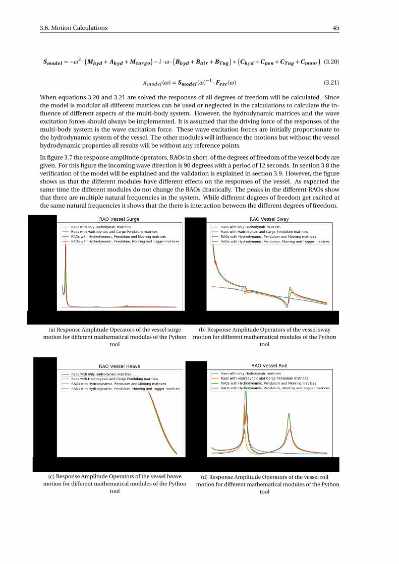
3.6. Motion Calculations 45
Smod el =−ω2 · (Mh yd + Ah yd +Mc ar g o)− i ·ω · (Bh yd +Bai r +BT ug
)+ (Ch yd +Cpen +CT ug +Cmoor
)(3.20)
xmodel (ω) = Smod el (ω)−1 ·Fexc (ω) (3.21)
When equations 3.20 and 3.21 are solved the responses of all degrees of freedom will be calculated. Sincethe model is modular all different matrices can be used or neglected in the calculations to calculate the in-fluence of different aspects of the multi-body system. However, the hydrodynamic matrices and the waveexcitation forces should always be implemented. It is assumed that the driving force of the responses of themulti-body system is the wave excitation force. These wave excitation forces are initially proportionate tothe hydrodynamic system of the vessel. The other modules will influence the motions but without the vesselhydrodynamic properties all results will be without any reference points.
In figure 3.7 the response amplitude operators, RAOs in short, of the degrees of freedom of the vessel body aregiven. For this figure the incoming wave direction is 90 degrees with a period of 12 seconds. In section 3.8 theverification of the model will be explained and the validation is explained in section 3.9. However, the figureshows us that the different modules have different effects on the responses of the vessel. As expected thesame time the different modules do not change the RAOs drastically. The peaks in the different RAOs showthat there are multiple natural frequencies in the system. While different degrees of freedom get excited atthe same natural frequencies it shows that the there is interaction between the different degrees of freedom.
(a) Response Amplitude Operators of the vessel surgemotion for different mathematical modules of the Python
tool
(b) Response Amplitude Operators of the vessel swaymotion for different mathematical modules of the Python
tool
(c) Response Amplitude Operators of the vessel heavemotion for different mathematical modules of the Python
tool
(d) Response Amplitude Operators of the vessel rollmotion for different mathematical modules of the Python
tool

46 3. Model description
motion for different mathematical modules of the Pythontool
(f) Response Amplitude Operators of the vessel yawmotion for different mathematical modules of the Python
tool
Figure 3.7: Response Amplitude Operators of the vessel six degrees of freedom for different mathematical modules of the Python tool
3.7. Significant MotionsWith the 12 degrees of freedom motion calculations completed the next step in motion predictions can bemade. First a wave spectrum must be calculated. This wave spectrum can be used to predict the significantmotion and a most probable maximum excitation and response over a certain time period.
First of all a wave spectrum must be calculated. Swell waves can often be described as a Pierson-Moskowitzspectrum and waves in the Northsea can be described as a JONSWAP spectrum. Equation 3.22 shows theequation for a Pierson-Moskowitz spectrum and the JONSWAP spectrum is given in equation 3.23. The JON-SWAP spectrum is essentialy a Pierson-Moskowitz spectrum with a peak enhancement function. In the JON-SWAP spectrum A is given by equation 3.24. Hs represents the significant wave height. The variable ωp
stands for the peak wave-frequency and ω stands for the wave frequency for which the energy is calculated.σ is equal to 0.07 if ωp ≤ω and equal to 0.09 if ωp >ω. The variable γ is the peak enhancement factor whichhas a default value of 3.3. for sea waves. Swell waves don’t need an peak enhancement factor thus this valueis set to 1 for swell waves.
SP M (ω) = 5
16·H 2
s ·ω4
p
ω5 ·e−54 ·
(ωpω
)4
(3.22)
S JON SW AP (ω) = (1−0.287 · ln(γ)
) ·( 5
16·H 2
s ·ω4
p
ω5 ·e−54 ·
(ωpω
)4)·γA (3.23)
A = e
(−0.5·
(ω−ωpσ·ωp
)2)
(3.24)
These wave spectra can be used to determine the motion response spectra. Equation 3.25 shows how theresponse spectra of the motions can be calculated. These response spectra can be used to calculate the mo-ments of the motions as shown in equation 3.26. The significant motions, in other words the mean value ofthe highest one-third part of the amplitudes, is calculated with the 0th moment, as shown in equation 3.27.
SX = |Xmodel |2 ·Sζ(ω) (3.25)
mnx =∫ ∞
0SX (ω) ·ωn ·dω wi thn = 0,1,2, ... (3.26)
X as = 2 ·pm0x (3.27)

3.8. Verification 47
The moments of the motion spectra can also be used to calculate the mean period and the average zero-crossing period as shown in equation 3.28 and equation 3.29 respectively. The zero-crossing period can beused to calculate the number of zero-crossings during a certain period of time which is shown in equation3.30. The number of zero-crossings and the 0th moment are used to calculate the most probable maximumof a motion during a certain time period. The equation for the most probable maximum is given in equation3.31[24].
T1X = 2π · m0x
m1x(3.28)
T2X = 2π · m0x
m2x(3.29)
N = t i meper i od
T2X(3.30)
MP MX =pm0x ·
√2 · ln(N ) (3.31)
In the Python model the integrals required to solve the moments of the motions from equation 3.26 are solvedwith the simpson’s rule. In section 2.2 is explained that the frequency step size in Shipmo can be chosen byvarying the range of the frequency in the calculations. For the significant motion calculations a hydrodynamicdatabase will be generated with a frequency range that fits the response spectra in order to calculate accurateMPM values. When the range is chosen too small some parts of the response spectra will be neglected inthe most probable maximum calculations. At the other hand, if the range is too large the peak values in theresponse spectra will be inaccurate which can also influence the most probable maximum calculations.
3.8. VerificationFor the verification the model is compared to the RAO data from Shipmo. When the cargo mass is equal to0 mton and the stiffness component of the crane wire is set to 0 the vessel RAOs of the model and the vesselRAOs of Shipmo should be exactly the same since all the hydrodynamic values are calculated with Shipmoand the influence of the pendulum is neglected. In figure 3.8 is shown that the RAOs from Shipmo and thePython tool are exactly the same.
(a) Response Amplitude Operators of the vessel surgemotion comparison of the calculation done by Shipmo and
by the Python tool
(b) Response Amplitude Operators of the vessel swaymotion comparison of the calculation done by Shipmo and
by the Python tool

48 3. Model description
(c) Response Amplitude Operators of the vessel heavemotion comparison of the calculation done by Shipmo and
by the Python tool
(d) Response Amplitude Operators of the vessel rollmotion comparison of the calculation done by Shipmo and
by the Python tool
(e) Response Amplitude Operators of the vessel pitchmotion comparison of the calculation done by Shipmo and
by the Python tool
(f) Response Amplitude Operators of the vessel yawmotion comparison of the calculation done by Shipmo and
by the Python tool
Figure 3.8: Response Amplitude Operators of the vessel six degrees of freedom comparison of the calculation done by Shipmo and thePython tool
Now that is established that the empty vessel calculations have the result that they are supposed to have theverification of the cargo pendulum motions can be started. With the help of stability software the hydrody-namic properties of the vessel will be calculated for the vessel in two different ways. In the hydrodynamiccalculations no coupling via the crane cable occurs. In the first calculation the cargo will be attached to thecrane top and in the second calculation the cargo will be placed at the CoG of the vessel. In both cases thevessel displacement will stay the same, which is important for the hydrodynamic properties of the vessel.However, there is a change in the metacentric height between the two stability calculations. The receivedvalues for draught and GM will be used in Shipmo to create two hydrodynamic database files. The hydrody-namic database file for the first case will be used to calculate the RAOs from the vessel without any pendulummotions since the influences from the cargo are applied on the GM of the vessel. In the second case the pen-dulum motions will be applied with the help of the Python tool created. In figure 3.10 the vessel RAOs forthe first and second case are plotted. The first case has one natural frequency in the vessel roll motion whichstands out. The second case has two notable natural frequencies. The first natural frequency is equal to thenatural frequency of the first case. The second national frequency is initiated by the pendulum motions. Thesimilarity in the roll natural frequency between the first and second case shows that the Python tool has a cor-rect influence on the natural frequencies. The difference in the resonance peaks of the natural roll frequencyis explained by the amount of energy in the system. In the first case all the energy from the wave excitationforce is translated to the vessel. In the second case the same amount of energy is applied to the vessel but the

3.8. Verification 49
vessel will also transfer some of the energy to the cargo pendulum motions. Therefore there is less energy inthe vessel roll motion. Hence the resonance peak is lower.
The eigenvector of the two natural frequencies that can be seen in figure 3.10d are plotted in figure 3.9. Inthis figure can be seen that both natural frequencies result in large excitations of the vessel roll motion andcargo sway motion. At the first natural frequency, around both degrees of freedom move inopposite directions of each other and at the second natural frequency both degrees of freedom move in thesame direction.
Figure 3.9: Eigenvector values of the two natural frequencies with a large influence on the vessel roll motion that occur in themulti-body model. The first natural frequency occurs around and the second natural frequency occurs around
In figure 3.10 can also be seen that the vessel surge, sway, pitch and yaw motion show peaks in the responsesaround and for the Python model where the cargo is modelled as a pen-dulum. In figure 3.11 the RAOs of the cargo surge and sway motion are given. In this figure can be seen thatthe cargo sway motion has strong similarities with the vessel roll motion. This will be further elaborated inchapter 4. In the figure can also be seen that the cargo surge motion has a large response aroundand the cargo sway motion has a large response around and . All these peaks in theresponses can be explained from the coupling between the vessel and cargo motions. When the cargo ismodelled as a mass applied to the crane tip there are only six degrees of freedom in the multi-body system.The motions of the cargo itself and the force introduced by these motions are not part of the equation andare thus neglected. When the cargo is modelled as a pendulum the multi-body system will contain out of12 degrees of freedom. The cargo motions are integrated in the system and new forces are introduced in themultibody system. These forces cause an interaction between the different degrees of freedom. The peakthat is found in figures 3.10a and 3.10e follow from the connection between the vessel surge, vessel pitch andcargo surge motion. The peaks in the vessel sway, vessel roll, vessel yaw and cargo sway motion follows froma connection between these degrees of freedom. In appendix C the equations of motion are given. In theseequations can be seen that the stiffness of the cargo pendulum introduces a restoring force that couples thesedegrees of freedom to each other in the multi-body system.

50 3. Model description
(a) Response Amplitude Operators of the vessel surgemotion. A comparison is made between conventional
calculations and the 12 degrees of freedom calculation.
(b) Response Amplitude Operators of the vessel swaymotion. A comparison is made between conventional
calculations and the 12 degrees of freedom calculation.
(c) Response Amplitude Operators of the vessel heavemotion. A comparison is made between conventional
calculations and the 12 degrees of freedom calculation.
(d) Response Amplitude Operators of the vessel roll motion.A comparison is made between conventional calculations
and the 12 degrees of freedom calculation.
(e) Response Amplitude Operators of the vessel pitchmotion. A comparison is made between conventional
calculations and the 12 degrees of freedom calculation.
(f) Response Amplitude Operators of the vessel yaw motion.A comparison is made between conventional calculations
and the 12 degrees of freedom calculation.
Figure 3.10: Response Amplitude Operators of the vessel six degrees of freedom for a comparison of the connection of the cargo. Acomparison is made between the method where the weight of the cargo is attached to the crane top and a method where the cargo is
modelled as a pendulum
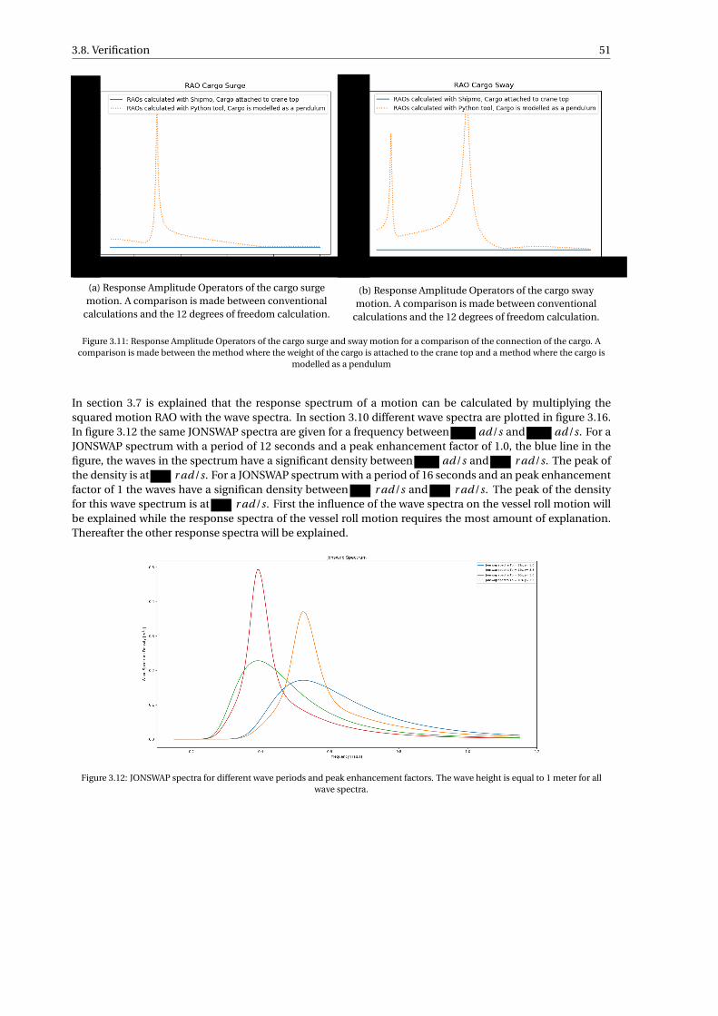
3.8. Verification 51
(a) Response Amplitude Operators of the cargo surgemotion. A comparison is made between conventional
calculations and the 12 degrees of freedom calculation.
(b) Response Amplitude Operators of the cargo swaymotion. A comparison is made between conventional
calculations and the 12 degrees of freedom calculation.
Figure 3.11: Response Amplitude Operators of the cargo surge and sway motion for a comparison of the connection of the cargo. Acomparison is made between the method where the weight of the cargo is attached to the crane top and a method where the cargo is
modelled as a pendulum
In section 3.7 is explained that the response spectrum of a motion can be calculated by multiplying thesquared motion RAO with the wave spectra. In section 3.10 different wave spectra are plotted in figure 3.16.In figure 3.12 the same JONSWAP spectra are given for a frequency between ad/s and ad/s. For aJONSWAP spectrum with a period of 12 seconds and a peak enhancement factor of 1.0, the blue line in thefigure, the waves in the spectrum have a significant density between ad/s and r ad/s. The peak ofthe density is at r ad/s. For a JONSWAP spectrum with a period of 16 seconds and an peak enhancementfactor of 1 the waves have a significan density between r ad/s and r ad/s. The peak of the densityfor this wave spectrum is at r ad/s. First the influence of the wave spectra on the vessel roll motion willbe explained while the response spectra of the vessel roll motion requires the most amount of explanation.Thereafter the other response spectra will be explained.
Figure 3.12: JONSWAP spectra for different wave periods and peak enhancement factors. The wave height is equal to 1 meter for allwave spectra.

52 3. Model description
The vessel roll motion RAO, given in figure 3.10d has large responses beteen and Bothfrequencies lie within the two energy density functions of the two different wave spectra. Thus when theresponses of the vessel roll motion are calculated for these wave spectra two peaks should be found in thevessel roll response spectrum. The other degrees of freedom of the vessel motion also have responses withinthe wave spectra and should also show responses. In figure 3.13 the responses of the vessel are given for wavespectra with 12 and 16 second periods. A period of 12 seconds corresponds to a frequency of r r ad/s anda period of 16 seconds corresponds to a frequency of r ad/s. The peak enhancement factor of both wavespectra is equal to 1.0. In these figures it is clear that the vessel roll motion show two peaks in its responsespectra for both wave spectra. However, the first peak of the response of the vessel roll motion for a JONSWAPspectrum with a period of 12 seconds is ratter small. This is explained by small amount of energy densityat the frequency of the first peak. The JONSWAP spectra with a period of 16 seconds has a higher density atthe first natural frequency of the vessel roll motion than at the second natural frequency. While the RAO ofthe vessel roll motion show larger responses at the natural frequency the combination of the larger density ofenergy at the first natural frequency results in almost evenly large responses for the two peaks for responseson a wave spectra with a period of 16 seconds and a peak enhancement factor of 16 seconds.
The vessel’s surge, sway and heave motion RAOs do not show any large peaks. The squared RAOs do There-fore not have extreme values. Therefore the responses of these degrees of freedom look a lot like the energydensity function of the JONSWAP spectra for a period of 12 and 16 seconds respectively. The peaks that canbe found in the RAOs can also be seen in the vessel response spectra, especially in the vessel surge motion.The vessel’s pitch and yaw motion do also not show large values in the RAOs however, the responses of thethree translations of the vessel are large for low frequencies and therefore they follow the wave spectra quiteaccurately. The RAO’s of the vessel pitch and yaw motion are low for small frequencies and increases till afrequency of after which the RAOs decreases again. These RAO’s show larger amplitudes at thefrequency at which the JONSWAP spectrum with a period of 12 seconds has the most amount of density.Therefore the Response spectra of the vessel pitch and yaw motion are larger for the JONSWAP spectrumwith a period of 12 seconds than the JONSWAP spectrum with a period of 16 seconds.
Although no mathematical equations are done to verify the response spectra of the motions the responsespectra behave exactly as is expected from the response spectrum. Therefore the response spectra can beused to calculate the Most Probable Maximum of the degrees of freedom in the multi-body system.
(a) Response spectrum of the vessel surge motion for waveswith according to JONSWAP spectra with a period of 12 and
16 seconds and a peak enhancement factor of 1.0.
(b) Response spectrum of the vessel Sway motion for waveswith according to JONSWAP spectra with a period of 12 and
16 seconds and a peak enhancement factor of 1.0.

3.8. Verification 53
(c) Response spectrum of the vessel Heave motion for waveswith according to JONSWAP spectra with a period of 12 and
16 seconds and a peak enhancement factor of 1.0.
(d) Response spectrum of the vessel Roll motion for waveswith according to JONSWAP spectra with a period of 12 and
16 seconds and a peak enhancement factor of 1.0.
(e) Response spectrum of the vessel Pitch motion for waveswith according to JONSWAP spectra with a period of 12 and
16 seconds and a peak enhancement factor of 1.0.
(f) Response spectrum of the vessel Yaw motion for waveswith according to JONSWAP spectra with a period of 12 and
16 seconds and a peak enhancement factor of 1.0.
Figure 3.13: Response spectra of the vessel motions. The responses are calculated for waves according to JONSWAP spectra with aperiod of 12 and 16 seconds and a peak enhancement factor of 1.0.
The most probable maximum calculations can be verified by comparing the most probable maximum calcu-lations for different wave heights. When the RAOs, wave period and peak enhancement factor are constantfor both MPM calculations and the wave height is the only variable, the MPM should have the same ratio asthe ratio between the different wave heights. When the wave height is doubled the MPM values should alsobe twice the original value. Table 3.5 shows that the MPM for waves with a spectra with a significant waveheight of two meters is exactly twice as large as the MPM for a spectra with a significant wave height of onemeter.

54 3. Model description
Table 3.5: Most probable maximum comparison where the RAOs are constant and the wave height is varied
Motion Hs = 1 m Hs = 2Vessel SurgeVessel SwayVessel HeaveVessel RollVessel PitchVessel YawCargo SurgeCargo SwayCargo HeaveCargo RollCargo PitchCargo Yaw
3.9. ValidationBigLift has the availability of a crane simulator. In this simulator a vessel with its cranes and cargo can beloaded. Since it is a simulator the input variables for wave data can be selected by the user. This can make thesimulator a useful tool to validate the Python tool. The simulator runs on the program Dolphin on version4.1. The simulator itself is not validated therefore the values of the simulator must not be seen as the onlytruth. Every five years Marin will have the software certified. Last year this is also done by DNV-GL. However,the Dolphin version that got certified was Dolphin 5.3. Strictly speaking the software of the crane simulatoris not certified. Since the version of 4.1 and 5.3 are running on the same principles the software of the cranesimulator might still be of use to validate the system. Another aspect of the crane simulator that might betroubling is the validation of the vessel behaviour in the similator. The vessels of BigLift in the similator arenot validated with model tests. the wave behavior of the vessel is derived from the Froude-Krylov forces inthe simulator.
Second order wave motions occur in the simulator. In the python model the frequency domain is used. Inthis frequency domain second order forces will not be taken into account and therefore the second ordermotions cannot be calculated. The second order motions from the similator can be filtered with the use ofa high-pass filter. Such a filter substracts all the motions with a period above 120 seconds. Manual testsshowed that a filter of 120 seconds shows good results in reducing the second order motions. In figure 3.14the unfiltered responses of the simulator of the cargo sway motion are given. Figure 3.15 the responses ofthe cargo sway motion that are filtered with a high-pass filter with a cutoff frequency of 120 seconds is given.These figures show that the large second order responses are filltered out and all responses oscillate aroundzero. The responses are definitely not linear, therefore the wave spectra are introduced in the Python model.However, the responses build-up and after a peak response decrease again. This is part of the resonance ofthe motions.
Figure 3.14: Unfiltered responses of the Cargo Sway motion in the crane similator. The waves have an angle of 90 degrees relative to thevessel. The significant wave height is 1 meter and the period is 12 seconds.

3.9. Validation 55
Figure 3.15: Filtered responses of the Cargo Sway motion in the crane similator. The second order wave forces are filtered a highpass-filter with a cutoff frequency of 120 seconds. The waves have an angle of 90 degrees relative to the vessel. The significant wave
height is 1 meter and the period is 12 seconds.
The data retrieved from the simulator can be used to calculate the most probable maximum of the responsesin the simulator. These most probable maximum values can be compared to the most probable maximumvalues of the Python model. First the timestamps of the zero-crossings must be calculated. This can bycomparing the signs of the responses between two consecutive timestamps. When the sign changes fromnegative to positive there is a zero-crossing. The maximum response can than be calculated between allzero-crossings of the responses. The maximum responses between all different zero-crossings can be used tocalculate the mean maximum as shown in equation 3.32. In this equation x represents the mean maximumvalue of the responses. N is the amount of zero-crossings and xi represents the maximum between two zero-crossings. The standard deviation between the different maximums and the mean maximum response can becalculated with equation 3.33. This standard deviation can be used to calculate the most probable maximumof the motions in the simulator as shown in equation 3.34.
x = 1
N −1·
N−1∑i=1
xi (3.32)
σmax =√∑N−1
i=1 (xi − x)2
N −1(3.33)
MP Msi mul ator =σmax ·√
2 · ln(N −1) (3.34)
Table 3.6: Most probable maximum comparison between crane simulator and python tool
Motion MPM SimulatorMPM Python Tool[Roll amp = 2 deg]
MPM Python Tool[Roll amp = 5 deg]
MPM Python Tool[Roll amp = 10 deg]
Vessel SurgeVessel SwayVessel HeaveVessel RollVessel PitchVessel YawCargo SurgeCargo SwayCargo HeaveCargo RollCargo PitchCargo Yaw

56 3. Model description
In table 3.6 the most probable maximum are given from the vessel and cargo responses in the simulator andthe responses calculated by the python tool. The first thing that stands out is the vessel and cargo surge mo-tions of the simulator. In the simulator the vessel surge motion is caused by forces that cannot be calculatedby a 2D-strip theory program like Shipmo. Therefore the python tool does not show these motions. Since thecargo surge motion is coupled to the vessel surge motion the cargo surge motion is also larger in the simu-lator. The second part that stands out is the vessel roll motion. This motion is a lot smaller in the simulatorthan in the Python tool. Different users of the simulator have stated that the damping in the simulator feelsexaggerated. This can explain the relative small roll motions of the vessel in the simulator. Since the vesselroll motion has a large influence on the cargo sway motion the value of this last degree of freedom is also alot higher for the calculations done with the simulator. Since the cargo roll, pitch and yaw motions are notcoupled to the pendulum motions these degrees of freedom will not be excited in the Python tool.
Since the simulator and the python tool both calculate the responses of the multi-body system with other ves-sel input values the answers of both methods will never equal to each other. However, besides the exceptionsmade in the previous paragraph, the order size of the results are equal for the two different methods.
3.10. Parameter InfluenceThe motions that occur due to wave excitation forces can be reduced in multiple ways. In section 2.2 isexplained that the wave forces and the motions of the multi-body system have a harmonic behaviour annatural frequency will occur. In section 2.7 is described how the natural frequencies of the multi-body systemcan be calculated. In section 2.3 till section 3.5 is explained how different constraints are implemented in thePython tool. When the waves during a lifting operation have the same frequency as, or a frequency close to,the natural frequency of one of the motions, the system can start to resonate. Since the multi-body systemhas different variables, such as vessel draught, vessel metacentric height, cargo mass, crane top positionand distance between crane top and cargo CoG the properties of the multi-body system can be varied. Thedifferent variables of the multi-body system can influence the different matrices in the multi-body system.When the mass and stiffness aspects of the multi-body system are changed the natural frequency of the multi-body will change.
Figure 3.16 shows the influence of the period and peak enhancement factors on the wave spectra calculatedwith equation 3.23. The figure shows that different wave periods and peak enhancement factors will influencethe wave spectra. Although the wave spectra are calculated for a specified period the energy is distributedover a large range of frequencies. Especially the range of the Pierson-Moskowitz spectra is large. The largerange of these spectra can influence the multi-body system even when the natural frequency is shifted. Thecombination of the vessel RAO and the wave spectrum determine how the multi-body system will respondduring certain operational conditions. A different natural frequency or wave spectrum can influence theresponse spectra and most probable maximum which are described in equations 3.25 and 3.31 respectively.
Figure 3.16: JONSWAP spectra for different periods and peak enhancement factors. Hs is equal to 1 meter for all spectra
For every lifting operation the variables in the multi-body will change, as well as the sea state during thelifting operations. Therefore it is important to calculate the natural frequencies of the multi-body system andtry to adjust these natural frequencies in order to shift the natural frequencies away from the wave periods

3.10. Parameter Influence 57
that occur during a lifting operation. When this can be done correctly, the responses of the vessel and cargomotions will be reduced. The Python tool can be used to calculate the influence of the variables on thenatural frequency of the multi-body system. In section 5.1 the influences of the variables on the naturalfrequencies will be calculated and explained. The mathematical and theoretical influence of these variableswill be explained in this section.
In chapter 4 calculations will be done to determine the baseline behaviour of BigLift’s Shipping vessel HappySky. Thereafter variables will be varied in chapter 5 to determine the sensitivity of these variables duringlifting operations. In this section the influence of the variables will be described in a mathematical way. Inchapter 5 the results of the sensitivity study will be shown.
The variables that are examined on their influence are the vessels draught, vessels metacentric height, cargomass, crane top X,Y and Z position and the length between crane top and cargo COG. The crane top X,Y and Zpositions as well as the length between the crane top and cargo COG will change without further explanation.The cargo mass will change as a percentage of the total weight in the system. This results in no displacementchange of the vessel for different cargo masses. In theory the vessel will have more ballast when the cargo hasa small weight than when the cargo has a heavy weight. In table 3.7 the variables and their remarks are given.
Table 3.7: Variables changed to study the influence
Variable Remarks
Cargo Mass The cargo mass will change as a percentage of the overall mass in the system.This results in a constant water displacement of the system, as long as thedraught is not changed. When the cargo mass is not varied it is kept constantat 3 % of the total mass in the system.
Vessel draught When the vessel draught changes the GM stays the same. While the waterlineand center of buoyancy change, the center of gravity will change in such away that the GM will stay the same. When the draught is not varied it is keptconstant at a value of 7 meters.
Vessel GM Changes without further explanation. When the GM is not varied it is keptconstant at a value of 3 meters.
Crane top X, Y and Z posi-tion
These values will be changed independently from each other. This is doneto carefully analyse the influence and interaction of the different rotations.When the crane X and Y positions are not varied they are kept constant at 0meters. When the crane Z position is not varied it is kept constant at 30 me-ters.
Crane cable length The length between the crane top and cargo COG will be varied between 10and 30 meters. When the crane cable length is not varied it is kept constant at20 meters.
3.10.1. Cargo MassIn a simple pendulum the mass should not influence the natural frequency of the system, while the naturalfrequency is equal to
√g /L. However, since this system is a coupled system other aspects besides the gravity
and sling length have influence on the natural frequency of the pendulum. When the mass of the cargoincreases the mass of the vessel decreases while the combined mass of the system has to stay constant. Thisresults in a change in the mass matrix of the vessel. However the displacement has to stay the same whilethe mass of the cargo influences the displacement of the vessel. Therefore the hydrodynamic database iscreated for the total displacement of the vessel and the mass matrix is adjusted to the to the mass of thecargo. Since the roll stiffness is related to GM ·∇ and the GM is constant the change in vessel mass should notaffect the vessel roll itself. However the coupled motions between the cargo and the vessel extent the originalequation of motions as explained in sections 3.3 and 3.6. Since the decreased vessel mass and increasedcargo mass should not influence on the uncoupled motions does this not mean that there is no influence at

58 3. Model description
all. While the matrix components C44, M44,C88 and M88 from appendix B do change with the same amountas its counterpart the whole 12 degrees of freedom stiffness matrix is more dense than the 12 degrees offreedom mass matrix. This difference in density does influence the natural frequencies of the multi-bodysystem. An increased cargo mass will reduce the overall stiffness values of the vessel roll degree of freedom.Thus increased cargo masses will reduce the natural frequency coupled to the vessel roll motion. The overallstiffness coupled to the pendulum sway motion will increase when the cargo mass increases which results ina higher natural frequency of the natural frequency coupled to the cargo sway motion when the cargo mass isincreased. In section 5.1.1 the exact influence of the cargo mass on the natural frequencies in the multi-bodysystem are shown.
3.10.2. Crane Cable LengthThe crane cable has a large influence on the restoring stiffness values of the pendulum motions as explainedin section 2.3. If the crane cable length increases the restoring stiffness decreases of both the restoring pendu-lum stiffness and crane cable stiffness. The coupling via the crane cable has influence on almost all the vesseland cargo degrees of freedom. When the restoring pendulum stiffness and crane cable stiffness is reduced thestiffness values of all degrees of freedom will be reduced. While the stiffness values are the numerator in thenatural frequency calculations the natural frequencies will reduce when the stiffness values are reduced. Thereduction of the stiffness values for all degrees of freedom will result in a reduction of all natural frequenciesof the multi-body system.
3.10.3. Crane Top Z PositionThe crane top Z position is used in the Python model to translate the rotations of the vessel body in trans-lations of the crane tip. When the crane top Z position is increased the vessel rotations will create largertranslation of the crane tip. At the same time are moments created by forces applied to the crane top also in-creased when the crane top Z position is increased. This results in larger rotational restoring stiffness valuesdue to the crane cable restoring stiffness calculations. The crane top Z position can have a large influencedue to these couplings. Dependent on the coupling between the different degrees of freedom the crane topZ position will increase or decrease the natural frequencies when the crane top Z position is increased. Inappendix C the complete equations of motion are given. In section 5.1.3 the influence of the crane top Zposition is calculated.
3.10.4. Crane Top Y PositionThe crane top Y position is, just like the crane top Z position, used in the Python model to translate the ro-tations of the vessel body in translations of the crane tip. When the position of the crane top is moved awayfrom mid ship the affect of the pendulum restoring stiffness due to rotations increases. However, due to theorientations of different motions, as explained in section 2.2, the stiffness affected by the Y position of thecrane top has, in opposite of the crane top Z position, a negative influence on the overall stiffness values ofthe equation of motion coupled to the vessel roll and cargo sway motion. The crane top Y position couples thevessel roll motion via the pendulum restoring stiffness to the vessel heave, pitch and yaw motions. Introduc-ing new stiffness components between these degrees of freedom will also couple the motions and exitationsin these directions. The complete equations of motion are given in appendix C. While the restoring pendu-lum stiffness is reduced when the Y position moves away from mid ship the value of the natural frequency isreduced. Since a positive and negative translation have the same affect on the stiffness components the nat-ural frequency is reduced with the same value when the Y position of the crane top changes. Since there canbe a phase difference between the vessel roll motion and pendulum sway motion the motions can reinforceeach other or diminish each other. The phase difference together with the location on the crane top positionscan influence the amplitude of the response. In section 5.1.4 the influences of the crane top Y position arecalculated.
3.10.5. Crane Top X PositionThe crane top X position has a corresponding physical influence as the crane top Y position. Only the degreesof freedom that are influenced by the crane top X position differ. While the sign of the crane top X position arecancelled in the calculation of the pendulum restoring stiffness for the vessel pitch and cargo sway motiona positive or negative sign will not influence the natural frequencies of these degrees of freedom. However,

3.10. Parameter Influence 59
the amplitude can be influenced by the positive or negative sign due to the phase difference between thevessel pitch and cargo surge motion. The crane top X position does also couple the vessel pitch and vesselyaw motion to the vessel roll motion via the pendulum stiffness matrix. Thus when the crane top X positionis not located above the centre of gravity of the vessel an interaction between different degrees of freedoms isintroduced.
The vessel hydrodynamical stiffness forces in the vessel roll direction are relatively small in comparison withthe hydrodynamical stiffness forces of the vessel pitch motion. Due to these larger stiffness forces the vesselpitch motion has much smaller amplitudes than the vessel roll motions. This can also be seen in figure 3.7.The pendulum restoring stiffness values can have the same order of magnitude as the vessel hydrodynamicroll stiffness values depending on the different variables. Due to this the lifting variables can influence thevessel roll motion a lot. However due to the large hydrodynamic pitch stiffness values the loading variableshave a much smaller influence on the vessel pitch motions. Due to the smaller influence the crane top Xposition is not supposed to create a difference in the pendulum stiffness values large enough to influencethe vessel pitch motion. While the vessel pitch motion will not be influenced by the crane top X position thecargo surge motion will have no new noticeable interactions with the other degrees of freedom in terms ofstiffness values. This should result in no variation of the cargo surge natural frequency when the crane topX position is varied. However, due to the difference in phases between the different degrees of freedom thecrane top X position can enhance or diminish the amplitude of the cargo surge motion. In section 5.1.5 theinfluence of the crane top X position on the multi-body system are calculated with the Python tool.
3.10.6. Vessel DraughtThe vessel draught is a variable that influences the water displacement of the vessel body. A larger displace-ment will result in larger mass values of the vessel body and larger added mass values of the vessel body.However, since a larger portion of the vessel hull is under water the hydrodynamic stiffness and damping val-ues will also increase since more water has to be displaced when the vessel body is in motion. Since both themass matrices and the hydrodynamic stiffness matrix are influenced by varying the draught and the influenceof the vessel draught on these matrices has to be calculated the relation between vessel draught and vesselmotions is not clear. When the mass matrices increase more than the stiffness values the natural frequencywill go down. When the hydrodynamic stiffness matrix increases more than the mass matrices the naturalfrequency will increase.
3.10.7. Vessel Metacentric HeightThe metacentric height, or GM, is a variable used to measure the stability of a vessel. In this case the vessel’stransverse metacentric height will be varried. The metacenctric height is the distance between the vessel’scentre of gravity and the vessel’s metacentre. When the vessel undergoes a roll motion the vessel’s centre ofbuoyancy shifts in the vessel’s transverse direction. The vessel’s metacentre can be determined by drawinga vertical line through the vessel’s centre of buoyancy for the upright position and the heeled position. Thelocation where both lines cross is the metacentric height as shown in figure 3.17. The metacentric height isalways located directly above the vessel’s centre of buoyancy.
Figure 3.17: schematic of the vessel’s metacentric height [39]
A large metacentric height results in a large stability of the vessel. The metacentric height has a large influenceon the hydrodynamic stiffness values of the vessel’s roll motion. In increased metacentric height results inlarger hydrodynamical stiffness values and should Therefore increase the natural frequency of the multi-bodymotions.

60 3. Model description
This metacentric height is the metacentric of the vessel without cargo in the crane. Which means that whenthe cargo mass is applied in the crane top the GM will go down as in simple 6 degrees of freedom RAO calcu-lations. In the Python tool the cargo is not implemented as a weight in the crane top but as a moving body.This moving body has an influence on the multi-body system. To get accurate results of the vessel and cargomotions the vessel’s metacentric height without cargo must used in the calculations. Otherwise the influenceof the cargo on the vessel’s stability will be used twice.

4Baseline Calculations
The model that is created for this research and explained in chapter 3 can be used to calculate the influenceof different variables on the motions of both the vessel and the cargo. The model is modular and differentconstraints and connections can be integrated or neglected in the calculations. The basic multi-body model,which includes the vessel hydrodynamic database and cargo pendulum interaction is used to calculate theinfluence of different variables on the motions of the whole system. The influence of mooring lines can beadded to the system to study the effect of this connection on the vessel and cargo motions. Cargo controlsystems can also be added to the main model which makes it possible to calculate the influence of suchsystems. However, before all these influences can be studied baseline values must be determined. In thischapter the baseline parameters and baseline responses will be explained and calculated. First the vesseldimensions will be explained in section 4.1. next the chosen wave direction of this study will be describedin section 4.2. Thereafter the natural frequencies and eigenvectors of the baseline case are studied in section4.3. Lastly the behaviour of the vessel with the baseline parameters will be explained with RAOs, responsespectra, phases and most probable maxima values.
4.1. Baseline CaseIn the study done to calculate the responses of the vessel and cargo the BigLift shipping vessel Happy Sky isused. In figure 4.1 a side view and top view drawing of the Happy Sky is shown. The Happy Sky has a lengthoverall of 154.8 meters. The moulded breadth is equal to 26.5 meters and the summer draught is 9.5 meters.The main deck is located 13.4 meters above the keel.
Figure 4.1: Side view and top view drawing of the BigLift Shipping vessel Happy Sky
61

62 4. Baseline Calculations
The Happy Sky is outfitted with two heavy lifting cranes. Each crane has a maximum capacity of 900 mton.The cranes have a maximum lifting height of 38.5 meters above the main deck and the radius of the crane isequal to 35.5 meters. The crane curves of the Happy Sky are shown in figure 4.2
Figure 4.2: Crane curves of the BigLift Shipping vessel Happy Sky
For a clear overview the baseline variables are given in table 4.1. The variables used in the baseline calcula-tions will now be discussed. First the origin of the coordinate system will be elaborated. The origin of themultibody system is the vessel’s centre of gravity. The centre of gravity is calculated by Shipmo. While themetacentric height is an input value of Shipmo as well as the draught and hullform the CoG correspondingto the GM can be calculated. The vessel rotational degrees of freedom will rotate around the centre of gravity.The centre of gravity is the most practical location of the origin while all rotational forces are related to thedistance to the centre of gravity and the location of the point of application does not require any translationcalculations. Shipmo calculated the centre of gravity for the baseline calculations at 74.3 meters from theafter perpendicular, 0 meters from the centre line and 9.7 meters from the keel. This means that the deck islocated 3.7 meters above the centre of gravity of the vessel. Although the vessel’s centre of gravity is the originthe cargo motions are relative to the cargo centre of gravity. In this way all degrees of freedom are plottedrelative to earth coordinate system.
The baseline vessel draught is equal to 7 meters. This draught is a normal draught during lifting operations.Some ports do have a draught restriction but 7 meter is a draught that is accessible most of the time. Thebasic vessel GM in these calculations is 3 meters. This value seems to be large for default GM values butthis is the GM value without any cargo attached to the crane as explained in section 3.2. When the cargo isattached in a conventional way the GM will go down drastically depending on the mass of the cargo and thelocation of the crane top. The crane top X an Y position will have a default value of 0 meters. This meansthat the cargo is lifted above the centre of gravity of the vessel. This is the most neutral place on the vessel.The crane top Z position has a baseline value of 30 meters. This height is an average height of the crane. Thesling length baseline value is equal to 20 meters. While the distance between the origin and the main deck isequal to 3.7 meters the cargo centre of gravity is located 6.3 meters above the deck. 6.3 meters seems like alarge distance. However, extremely large cargoes can have their centre of gravity 6.3 meters or more above thebottom of the cargo. In the baseline case it is assumed that there is enough clearance between the vessel andthe cargo but in detailed operational calculations the clearance must be taken into account. A sling length of20 meters is a length where the cargo motions have a significant influence due to the restoring stiffness of thecrane. The baseline value for the cargo mass is equal to 3 % of the total weight in the system. This is not themaximum weight the vessel can lift with one crane but it still is a significant weight. The weight is dependingon the vessel draught. With a draught of 7 meter the weight is approximately 650 mton. Mooring lines willnot be included in the baseline behaviour and sensitivity study. In section 5.2 the influence of mooring linesis calculated and explained. With all these variables the RAO calculations as described in section 3.6 can beperformed. The results of the baseline calculations will be discussed in section 4.4.

4.2. Wave Direction 63
Table 4.1: Values of the variables used in the baseline case.
Variable ValueVessel Draught 7 metersVessel GMt 3 metersCrane Top Z position 30 metersCrane Top X position 0 metersCrane Top Y position 0 metersCrane cable length 20 metersCargo Weight 3 %
4.2. Wave DirectionAs explained in section 3.6 the responses of the multi-body system are calculated from the excitation forcesand the dynamical model of the multi-body system. The program Shipmo is used to calculate the vesselhydrodynamics and the wave excitation forces. These excitation forces are dependent on the wave direction,vessel speed and hull form. The hull form will stay constant in all calculations. The wave direction is thedirection of the waves in comparison with the vessel heading. Since the vessel speed is assumed to be equal tozero, as explained in section 2.2, the encounter direction of the waves will be equal to the wave direction. Theencounter direction is the direction from which the waves apply forces to the vessel. During lifting operationsthe vessel will have no speed. The relative speed to the water due to current will be neglected. Since this thesisfocuses on the vessel behaviour and not on the waves behaviour the influence of current are not taken intoaccount. Thus the hull form and vessel speed will not change in the sensitivity calculations. However, thewave direction is a variable that can change. In appendix D RAOs for all degrees of freedom for three differentwave directions are given. In figure 4.3 the RAOs for the vessel roll and cargo sway motion are given. Thefirst wave direction is equal to 90 degrees. These waves, called beam seas, travel in perpendicular directionof the vessel direction. The second RAO that is given are waves with an angle of 45 degrees. The last RAOthat is given are waves with a direction of 0 degrees. These waves encounter the vessel at the stern. Thevessel roll motion and cargo sway motion are the two degrees of freedom that are influenced the most dueto wave excitation forces. Both degrees of freedom influence each other which explains the large responses.The complete equation of motion is given in appendix C. The equation of motion explain the full relationbetween vessel roll and cargo sway motions. Since these two degrees of freedom show the largest responsesthe RAOs are given in figure 4.3. Due to the same reason these two degree will be the focus of the sensitivitystudy and damping study. In the RAOs can be seen that the waves with an angle of 90 degrees create thelargest responses. Especially the second natural frequency of the cargo sway motion that can be seen in thefigures is extremely large for waves with an angle of 90 degrees.
In figure 4.4 the vessel pitch and cargo surge motion RAOs are given. The cargo surge motion only has onenatural frequency within ad/s and r ad/s. This natural frequency has a small frequency on the ves-sel’s pitch motion but the interaction is not as extreme as the interaction between the vessel roll and cargosway motion. The length of the vessel causes a large longitudinal metacentric height. Due to this long lon-gitudinal metacentric height the vessel pitch degree of freedom generates a lot of restoring forces due to thehydrodynamic properties. Therefore the vessel pitch motion will not show large responses as the vessel rollmotion. An interesting phenomenon in figure 4.4b are the larger responses at the natural frequency for waveswith an incoming angle of 45 degrees than the for waves with an incoming wave angle of 90 degrees. Theselarge responses can be explained from the larger responses of the vessel surge and pitch motion at this fre-quency. The vessel surge and pitch motion are coupled to the cargo surge motion. At the natural frequencythe responses of these vessel motions are larger which results in a larger response on the cargo surge motion.
The largest influence on the cargo surge and cargo sway motion is the pendulum restoring forces. Due tothese restoring forces a mathematical coupling between the vessel and cargo is created. While the restoringstiffness originates from the same variables for both degrees of freedom the influence of different lifting con-figurations and cargo control systems should be proportional. While the cargo sway motion is more complexdue to the strong connection with the vessel roll motion the vessel roll and cargo sway motion will be themain focus of the sensitivity and cargo control systems study. The restoring stiffness in cargo surge directionhas the same order size as the restoring stiffness in the cargo sway motion direction. However, the hydrody-namic stiffness in the vessel pitch direction is a lot larger than the hydrodynamic stiffness in the vessel rolldirection. Therefore the influence of the cargo surge motion on the vessel pitch motion is a lot smaller than

64 4. Baseline Calculations
the influence of the cargo sway motion on the vessel roll motion. In the RAOs shown in figure 4.3 can beseen that the waves with an angle of 90 degrees create the largest responses for the vessel roll and cargo swaymotion. Therefore an wave angle of 90 degrees will be used to calculate the influence
(a) Vessel roll motion RAO for different wave directions (b) Cargo sway motion RAO for different wave directions
Figure 4.3: Influence of different wave angles on the vessel roll motion and cargo sway motion RAO
(a) Vessel pitch motion RAO for different wave directions (b) Cargo surge motion RAO for different wave directions
Figure 4.4: Influence of different wave angles on the vessel pitch motion and cargo surge motion RAO
Figure 4.5: Influence of different wave angles on the vessel surge motion RAO.

4.3. Natural Frequencies and Eigenvectors 65
4.3. Natural Frequencies and EigenvectorsIn the previous sections is explained what the baseline variables are and which wave direction will be fo-cused on during the study. In chapter 2 is explained that the eigenvectors can be used to calculate the ratio ofresponse between different degrees of freedom at the different natural frequencies in the system. The eigen-vectors can also tell if any relation between the different degrees of freedom is missed in the previous section.Therefore the natural frequencies and eigenvectors will be calculated.
In table 4.2 the natural frequencies of the multi-body system with the baseline variables are given. The firstnatural frequency is fairly high and will not be excited by the waves encountered during lifting operations.Natural frequencies 7, 8 and 9 are so low that they will also not excitate the vessel during lifting operations.This leaves the second till the sixth natural frequency in a frequency range that can occur during lifting oper-ations.
Table 4.2: Natural frequencies of the baseline multi-body system
Natural frequency Frequency [rad/s]1234567 -068 -089 -08
In figure 4.6 the eigenvectors of the natural frequencies 2 till 6 are plotted. The values of these eigenvectorsare non-dimensional since they give a relation between the responses of different degree of freedom in themulti-body system. However, it is important to notice that there is a difference between translations androtations. Degree of freedom 1 til 3 and 7 till 9 give the translations. Thus these values are coupled to atranslation in a certain unit length. Degree of freedom 4 till 6 and 10 till 12 are angular responses. Thus thesevalues are coupled to an angular motion. While the crane wire is assumed to be connected to the cargo centreof gravity no rotations are introduced to the cargo body in the baseline calculations. Therefore no rotationsare plotted in figure 4.6. The translations and rotations are coupled in such a way that the scale on the axisfor a translation of one metre is equal to a rotation of 1 degree on the same scale.
Natural frequency number 2 and 6 correspond to the large responses seen in the vessel roll and cargo swaymotions in figure 4.3. The eigenvectors do also show that the other degrees of freedom have little interactionwith these two natural frequencies. Natural frequency number 3 corresponds to the large responses in thecargo surge motion in figure 4.4b. This eigenvector does also show that there is little interaction between thecargo surge motion and the other degrees of freedom at this natural frequency. The two remaining naturalfrequencies within the operational wave frequency range are natural frequency number 4 and 5. The eigen-vectors of these natural frequency show that these two natural frequencies excitate the vessel heave, vesselpitch, cargo surge and cargo heave motion. However, these natural frequencies do not have the same order ofamplitudes as the other natural frequencies shown in figures 4.3 till 4.5. These two RAOs seem to correspondto the natural frequency of the vessel pitch motion. Even though the amplitude of the vessel pitch motionRAO is quite broad the amplitude of the vessel pitch motion RAO is relative small. Because of this the influ-ence of the vessel pitch motion on the other degrees of freedom is also relatively small and no large peakscan be found at the 4th and 5th natural frequency. The eigenvectors do show that the cargo surge motion hasa certain amount of coupling with the vessel pitch and vessel heave motion. However the coupling is a lotsmaller for these degrees of freedom than the coupling between the vessel roll and cargo sway motion. Whilethe responses on the 4th and 5th natural frequency are quite small in comparison with the other naturalfrequencies the study can be performed on the vessel roll and cargo sway motion.

66 4. Baseline Calculations
Figure 4.6: Eigenvectors of natural frequencies 2 till 6 of the baseline model
4.4. Baseline BehaviourIn this section the baseline behaviour in terms of RAOs and significant motions will be described. In figure4.7 the RAO of the vessel roll motion is plotted. In this figure the RAO is plotted for a frequency range between
and r ad/s. As explained in section 2.2 a fairly big stepsize is the result of such a large frequency range.Therefore the RAO is plotted in figure 4.8 with a smaller frequency range. This results in a more detaild RAOgraph. In figure 4.7 the peaks are angular and sharp while the peaks in figure 4.8 are more smooth. In figure4.7 it is clear that the two dominating frequencies for the roll motion can be found around r ad/s and
r ad/s. This corresponds to the natural frequencies calculated in the previous section. When a closerlook is taken at the height of these resonance peaks in the different figures it becomes clear that there is alsoa difference in the maximum response. The RAO value at the natural frequency of r ad/s in figure 4.7 isclose to deg /m while the same RAO has a value close to deg /m in figure 4.8a. At the second naturalfrequency of r ad/s the value of the RAO is equal to deg /m in figure 4.7 while figure 4.8b showsalso a value of deg /m. The difference at the first natural frequency is caused by the stepsize of the wavefrequencies. The exact value of the natural frequency lies in between two steps used to plot figure 4.7. Thesmaller stepsize in the detailed calculations make it possible to calculate a more exact value. The secondnatural frequency is close to a step of the wave frequency used in figure 4.7. As a result the value of the RAOamplitude is quite accurate. The inaccuracy at the first natural frequency shows that detailed calculationswith small stepsizes are important. Therefore the responses will be calculated for a range between and
r ad/s. Detailed graphs with smaller ranges will be created to show the RAOs of multi-body system.

4.4. Baseline Behaviour 67
Figure 4.7: RAO of the vessel roll motion with the baseline variable values
(a) Vessel roll motion RAO for a frequency betweenand 0.55 /s
(b) Vessel roll motion RAO for a frequency betweenand rad/s
Figure 4.8: A detailed vessel roll motion RAO for frequencies between and rad/s and between and rad/s
Figure 4.9: RAO of the cargo sway motion with the baseline variable values

68 4. Baseline Calculations
(a) Cargo sway motion RAO for a frequency betweenand rad/s
(b) Cargo sway motion RAO for a frequency betweenand rad/s
Figure 4.10: A detailed cargo sway motion RAO for frequencies between and rad/s and between and rad/s
The phases of the different degree of freedom can explain more about the natural frequencies and to whichmotions these natural frequencies are coupled. In section 2.6 is explained that the stiffness values, and thusthe restoring force, coupled to a degree of freedom are the biggest influence on a motion when the drivingfrequency is smaller than the natural frequency. At the same time will the inertia forces influence the mo-tions of a degree of freedom the most when the driving frequency is larger than the resonance frequency. Therestoring forces are coupled to the displacement of a body and the inertia forces are related to the accelera-tions of a body. Equations 2.7 and 2.9 show that the translation and accelerations act in opposite directionsin harmonic oscillations. Due to these directions of the translations and accelerations the phase of a motionwill change around the natural frequencies. The phases of the vessel roll motion and cargo sway motion aregiven in figure 4.11. In these figures the phases the motions themselves are given. The motions, and thus theirphases, are a result of the a multiplication of the squared combined ship system with the excitation force. Insection 3.2 is explained that the waves exert forces on the vessel. While the waves exert forces on all six de-grees of freedom the phases of the wave forces can not be deducted from the vessel and cargo responses. Infigure 4.12 the phases of the wave excitation force in the vessel sway and vessel roll direction are given. Thesefigures show that the wave forces in different directions change in a different way over a range of frequencies.
In figure 4.11 can be seen that the phases of the vessel roll motion change drastically around r ad/s, thusaround the first natural frequency. The phase of the cargo sway motion does also change at the first naturalfrequency at r ad/s. At the second natural frequency, at r ad/s, the phase of the vessel roll motionand the cargo sway motions changes drastically again. These changes in the phase confirm that the naturalfrequency calculations are done correctly since the phases should change around the natural frequency asexplained in section 2.6. However, big changes in the phase of a motion is not limited to the frequency. At adriving frequency of r ad/s the phase of the cargo sway motion changes while the phase of the vesselroll motion does not change. This change can be explained by the anti-resonance that occurs around thisfrequency for the cargo sway motion. In figure 4.9 and figure 4.10a a small dip in the response can be seen atthis frequency. This indicates that anti-resonance occurs as explained in section 2.6. For driving frequenciesbelow r ad/s the phase of the vessel roll and cargo sway motion are close to equal. This indicates thatthe both degree of freedom move in the same direction. The anti resonance that occurs at r ad/s causesa change in the phase of the cargo sway motion. Which results in a motion in an opposite direction of thevessel roll motion. At the first natural frequency both degree of freedom change their face with the samevalue. This keeps the different in direction of the motion. At r ad/s anti resonance occurs in the vesselroll motion. This can also be seen in figure 4.7. Due to this change in phase after the anti resonance the vesselroll motion and cargo sway motion have the same phase again at the second natural frequency. This causesthe two degrees of freedom to move in the same direction.

4.4. Baseline Behaviour 69
(a) Phase of the vessel roll motion for the multi-bodymodel with baseline variables
(b) Phase of the cargo sway motion for the multi-bodymodel with baseline variables
Figure 4.11: Phase of the vessel roll and cargo sway motion for the different frequencies within the range in which the RAOs arecalculated. The Phases are calculated for the responses of the multi-body model with the baseline variables
(a) Phase of the wave excitation force in vessel swaydirection
(b) Phase of the wave excitation force in vessel rolldirection
Figure 4.12: Phase of the wave excitation force in vessel the vessel sway and vessel roll direction.
The RAOs given in figures 4.7 till 4.10 can show great insight in the behaviour of the vessel. However, duringlifting operations the waves can vary. As stated in the problem statement swell waves causes a lot of problemsfor BigLift Shipping. The response spectra can be used to study how the multi-body system will respondin a certain wave spectrum. Swell waves are waves with a period between the 12 and 16 seconds. In figure4.13 The different wave spectra are plotted. A JONSWAP spectrum with a peak enhancement factor of 1 isequal to a Pierson-Moskowitz spectrum. Such a spectrum can be used to generate a approximation of a swellspectrum. In figure 4.14 the response spectra of the vessel roll and cargo sway motion are drawn for differentswell periods. In these figures can be seen that the higher the wave period the less influence the naturalfrequency of r ad/s has. A frequency of r ad/s corresponds to a period of seconds. Thereforeit is easy to assume that the swell period of 14 seconds causes the largest response in the response spectrum.However, since the wave spectra with a period of 16 seconds has a high energy density the response spectrumrelated to this wave spectrum is also large. However the response around the second natural frequency is alot smaller for the wave spectra with a higher period.

70 4. Baseline Calculations
Figure 4.13: JONSWAP spectra for different wave periods. The wave periods are varied between 12 and 16 seconds. The wave height isset to 1 meter and the peak enhancement factor is equal to 1.
(a) Response spectrum of the vessel roll motion for themulti-body model with baseline variables
(b) Response spectrum of the cargo sway motion for themulti-body model with baseline variables
Figure 4.14: Response spectra of the vessel roll and cargo sway motion for waves with a period of 12, 14 and 16 seconds. The Phases arecalculated for the responses of the multi-body model with the baseline variables
In table 4.3 the most probable maximum are given for the different swell spectra. The wave height of theswell spectra is taken equal to 1 meter. This makes the MPM values a MPM per meter wave height. Theresponse figures showed that the response spectra for waves with a period of 14 and 16 seconds showed largeresponses. Due to the high responses of the vessel roll motion around the first natural frequency the MPM ofthe vessel roll motion is slightly larger for waves with a period of 16 seconds than for waves with a period of 14seconds. While the cargo sway motion shows larger responses than the vessel roll motions around the naturalfrequency of r ad/s the response of the cargo sway motion around this frequency has a larger influenceon the cargo sway motion MPM than the response of the vessel roll motion on the roll motion MPM. Due tothis large influence of the response around the second natural frequency the MPM is the largest for waveswith a period of 12 seconds.
Table 4.3: MPM values of the vessel roll and cargo sway motion for baseline variables. The wave height is taken equal to 1 meter.
Configuration MPM Tp = 12 MPM Tp = 14 MPM Tp = 16Vessel Roll Cargo Sway Vessel Roll Cargo Sway Vessel Roll Cargo Sway[deg] [m] [deg] [m] [deg] [m]
Baseline variables

5Sensitivity of lifting variables
The multi-body model is created and the baseline behaviour of the vessel and cargo is studied. The firststep in reducing the responses of the multi-body model is studying the influence of the different variablesduring a lifting operation. In section 5.1 different variables of the multi-body system will be changed and theirinfluence on the multi-body system will be studied. While the variables will have influence on the differentmass and stiffness values in the multi-body system the variables will influence the natural frequencies in themulti-body system. The rate of change of the natural frequencies can show how much influence a variable hason the responses of the multi-body system. In section 5.2 the influences of mooring lines on the multi-bodysystem will be worked out.
5.1. Influences of Lifting VariablesThe variables that are examined on their influence are the vessels draught, vessels metacentric height, cargomass, crane top X, Y and Z position and the length between crane top and cargo centre of gravity. For everyvariable a minimum of 5 different values will be used and only one variable will be changed per calculation.For every variation the natural frequency and resonance peak of vessel roll and cargo motions will writtendown. When the displacement is changed it is assumed that the GM will stay the same. This means thattheoretically the values of KB, BM and KG will change in such a way that the GM value will be equal fordifferent draughts. As said the GM and displacement will have 5 different values. This means that at first 5different Shipmo hydrodynamic database files must be created for each of these two variables. With thesedatabases the natural frequencies of the 12 degrees of freedom system be calculated. These results will beused to calculate the range of frequencies for the roll and pendulum motions. When the frequency range ofinterest is determined RAO databases with small frequencies steps can be made and used to create accuratenatural frequency calculations. The crane top X, Y and Z positions as well as the length between the crane topand cargo COG will change without further explanation. The cargo mass will change as a percentage of thetotal weight in the system. This results in no displacement change of the vessel for different cargo masses. Intheory the vessel will have more ballast when the cargo has a small weight than when the cargo has a heavyweight. In table 5.1 the variables and their remarks are given.
71

72 5. Sensitivity of lifting variables
Table 5.1: Variables changed to study the influence
Variable Remarks
Vessel draught When the vessel draught changes the GM stays the same. While the waterlineand center of buoyancy change, the center of gravity will change in such away that the GM will stay the same. When the draught is not varied it is keptconstant at a value of 7 meters.
Vessel GM It is assumed that the vessel GM changes without influencing the other vari-ables. In theory the vessel’s KB, BM and KG will change in such a way that theGM changes but the other variables stay constant. When the GM is not variedit is kept constant at a value of 3 meters.
Crane top X, Y and Z posi-tion
These values will be changed independently from each other. This is doneto carefully analyse the influence and interaction of the different rotations.When the crane X and Y positions are not varied they are kept constant at 0meters. When the crane Z position is not varied it is kept constant at 30 me-ters.
Crane cable length The length between the crane top and cargo COG will vary between 10 and 30meters. In practice large crane cable length will cause a collision between thevessel’s deck and the cargo. However, mathematically and theoretically thevalues can be used to study the influence of the crane cable length. When thecrane cable length is not varied it is kept constant at 20 meters.
Cargo Mass The cargo mass will change as a percentage of the overall mass in the system.This results in a constant water displacement of the system, as long as thedraught is not changed. When the cargo mass is not varied it is kept constantat 3 % of the total mass in the system.
For every variable the natural frequencies are calculated in a general way. These calculations show the differ-ent ranges of the natural frequencies. While it is a multibody system with 12 degrees of freedom 12 differentnatural frequencies can occur. However, 2 motions are dominant in the graphs. Those motions are the rollmotion and the pendulum sway motion. Both motions influence each other which causes two big excitationsand two different frequencies. Since the equation of motions is solved in a range from 0.1 to 2.6 radians persecond with a frequency step of 0.0125 radians per second a general frequency range can be found. In thisstudy it became clear that the natural roll frequency occurs somewhere between the 0.35 and 0.60 radians persecond and the natural pendulum frequency occurs between 0.65 and 1.05, Therefore a detailed calculationis done for these ranges with a frequency step of 0.001 radians per second.
5.1.1. Cargo MassThe cargo mass is varied between 0% and 5% of the total mass of the system. In table 5.2 the values of thenatural frequencies for different masses are given as well as the amplitude of the resonance peak for the vesselroll and cargo sway motion. In figure 5.1 the natural frequencies are plotted in relation with the cargo massas % of all the mass in the system. In section 3.10.1 the influences of the cargo on the multi-body systemare explained in detail. When the cargo mass is changed while all other variables are kept constant the cargomass has an interesting effect on the multi-body system. While the draught of the vessel is kept constant theincreased cargo mass will change the mass components that influence the natural frequencies coupled to thevessel roll motion and cargo sway motion in two different ways. While an increased cargo mass reduces thestiffness of the components coupled to the vessel roll motion the natural frequency coupled to this motionwill decrease when the cargo mass increases. At the other hand an increased cargo mass increases the stiffnesscomponents coupled to the cargo sway motion which increases the natural frequency introduced due to theequation of motion of the cargo sway motion. The natural frequencies shown in table 5.2 and figure 5.1 showthat this occurs for these two natural frequencies.

5.1. Influences of Lifting Variables 73
While both the vessel roll motion and cargo sway motion have a strong connection to each other, as explainedin section 4.3, the natural frequencies coupled to both degree of freedom will also influence the other degreeof freedom.
In table 5.2 can be seen that the responses show large amplitudes. While these responses are large it doesnot mean that these responses occur. Due to linearization the peak values can occur in a frequency domaincalculation but in reality other forces prohibit the large amplitudes from existence. At the same time doenvironmental waves exist out of multiple linear waves, as explained in section 2.2. Due to the nature of thewave spectra the multi-body system will not be excited at the pure natural frequency. Besides these soothingaspects of the high amplitudes the change in amplitudes the effect of the cargo mass on the responses ofthe vessel roll and cargo sway motion. A heavier cargo reduces the amplitude of both the vessel roll andcargo sway motion for the first natural frequency. In figure 4.6 is shwon that at this natural frequency the twodegrees of freedom move in opposite direction of each other. Due to the heavier weight the wave forces willexcitate the two bodies to a smaller amplitude before an equilibrium is met. At the second natural frequencythe two degrees of freedom move in the same direction as shown in figure 4.6. While the cargo is heavier theinfluence of the cargo motions will influence the vessel roll motion in a more significant way. At the otherhand a heavier cargo results in a lower amplitude of the cargo sway motion at the second natural frequency.Due to the heavier cargo a smaller amplitude is a result of the wave excitation force.
Table 5.2: Influence of cargo mass on the roll and pendulum natural frequencies and amplitude of the resonance peaks.
Cargo MassFirst naturalfrequency
AmplitudeVessel Roll
AmplitudeCargo Sway
Second naturalfrequency
AmplitudeVessel Roll
AmplitudeCargo Sway
[% total mass] [rad/s] [deg] [m] [rad/s] [deg] [m]0 - - -0.512345
(a) Relation between the cargo mass and the natural rollfrequency
(b) Relation between the cargo mass and the naturalpendulum frequency
Figure 5.1: Relation between cargo mass and the natural frequencies of the roll and pendulum motions
5.1.2. Crane Cable LengthThe crane cable length is varied between 10 and 30 meters. The natural frequencies and peak values of theresonance for the different crane cable lengths can be found in table 5.3. In figure 5.2 the natural frequenciesof the roll and pendulum motions are plotted. As explained in section 3.10.2 the crane cable length has asignificant influence on the restoring stiffness values of the crane cable connection. The crane cable lengthinfluences the natural frequency of both the roll and pendulum motions. As shown in the figures below is theinfluence on the second natural frequency larger than on the first natural frequency. While the first naturalfrequency is mainly excited due to the vessel roll motions the change in restoring stiffness has a relativelysmall influence. The hydrodynamic stiffness of the vessel roll motion is larger than the restoring stiffness of

74 5. Sensitivity of lifting variables
the crane cable connection. On the second natural frequency the restoring stiffness has the largest influenceon the natural frequency. Hence, the influence of the crane cable length on the second natural frequency is alot larger.
The first natural frequency is mainly excited due to the vessel roll motion. While a short crane cable lengthcreates a large angle between the crane tip and cargo centre of gravity a lot of restoring forces are generated.When the crane cable length increases the angle between the crane top and centre of gravity decreases withthe same relative horizontal distance between crane tip and cargo centre of gravity. The large angle andrelative large restoring force explains the large amplitude for the small crane cable lengths and the smallamplitude for the large crane cable lengths. The second natural frequency is mainly excited due to the naturalfrequency of the cargo sway motion. Due to the longer crane cable length the restoring stiffness is reducedand a larger roll motion is required to reach an equilibrium in stiffness values. At the same time the amplitudeof the cargo sway motion RAO is reduced at the second natural frequency for longer crane cables.
Table 5.3: Influence of crane cable length on the roll and pendulum natural frequencies and amplitude of the resonance peaks.
Crane cablelength
First naturalfrequency
AmplitudeVessel Roll
AmplitudeCargo Sway
Second naturalfrequency
AmplitudeVessel Roll
AmplitudeCargo Sway
[m] [rad/s] [deg] [m] [rad/s] [deg] [m]1015202530
(a) Relation between the crane cable length and thenatural roll frequency
(b) Relation between the crane cable length and thenatural pendulum frequency
Figure 5.2: Relation between crane cable length and the natural frequencies of the roll and pendulum motions
5.1.3. Crane Top Z PositionThe position of the crane top in Z direction is varied between 20 and 60 meters. In table 5.4 the values of thenatural frequencies for the different Z positions as well as the amplitude of the resonance peaks are given.The natural frequencies for the different Z positions of the crane top are plotted in figure 5.3. In section 3.10.3is explained that the crane top Z position has a lot of influence on different coupling terms in the equationof motion. An increase of the crane top Z position increases the moments created by the restoring stiffnessof the crane cable connection. However, the crane top Z position does also determine how far the cranetop is translated due to the vessel roll motion. On the first natural frequency the coupling has a negativeeffect. When the crane top Z position is increased the natural frequency is decreased. While the first naturalfrequency is mainly dependent on the vessel roll motion the larger translations of the crane top result in largerinfluence of the cargo on the stability of the vessel. In conventional calculations the metacentric height of thevessel is adjusted relatively to the crane tip height. In this dynamical model the same influence occurs. Thesecond natural frequency is mainly dependent on the restoring stiffness of the crane cable coupling. Whilethe crane top Z position is increased the restoring moment that couple the vessel roll motion to the cargo swaymotion is increased. Therefor the natural frequency is increased when the crane top Z position is increased.

5.1. Influences of Lifting Variables 75
The larger values of the crane top Z position will increase the translations of the crane top due to the vessel rollmotion. These larger translations will cause a larger relative distance between the crane top and the centreof gravity of the cargo. While the first natural frequency is mostly generated due to the vessel roll motionthe amplitude of the cargo sway motion increases when the crane top Z position is increased. The secondnatural frequency is mainly generated by the cargo sway motion. A larger crane top Z position will result inlarger moment arms. With larger moment arms a smaller restoring force, or excitation is required to generatethe same moment. This results in smaller amplitudes around the second natural frequency for larger cranetop Z positions.
Table 5.4: Influence of the crane top Z position on the roll and pendulum natural frequencies and amplitude of the resonance peaks.
Crane topZ position
First naturalfrequency
AmplitudeVessel Roll
AmplitudeCargo Sway
Second naturalfrequency
AmplitudeVessel Roll
AmplitudeCargo Sway
[m] [rad/s] [deg] [m] [rad/s] [deg] [m]2030405060
(a) Relation between the crane top Z position and thenatural roll frequency
(b) Relation between the crane top Z position and thenatural pendulum frequency
Figure 5.3: Relation between crane top Z position and the natural frequencies of the roll and pendulum motions
5.1.4. Crane Top Y PositionThe position of the crane top in Y direction is varied between -50 and 50 meters. The outreach of the craneis 35 meter. While the cranes are located at the starboard side of the vessel the maximum outreach to portside is approximately 23 meters and the outreach to starboard side is approximately 47 meters. Thus not allY positions studied are physically possible. However the larger crane top Y positions are used to create moremathematical data. The natural frequencies and peak values of the resonance for the different Y positionsof the crane top can be found in n table 5.5. In figure 5.4 the natural frequencies of the roll and pendulummotions are plotted. As explained in section 3.10.4 the crane top Y position has a negative effect on the vesselroll and cargo sway motion stiffness components. Due to this negative effect the natural frequencies of thevessel roll and cargo sway motion will decrease.
While the positive or negative sign of the crane top Y position does not influence the natural frequencies ofthe multi-body system the amplitude is influenced by the different signs. In section 3.10.4 is explained thatthe phases of both motions in combination with the crane top Y position can cause an enhancement of theamplitude or a reduction of the amplitude. In this case the negative crane top Y positions have a smalleramplitude than the positive crane top Y positions.

76 5. Sensitivity of lifting variables
Table 5.5: Influence of the crane top Y position on the roll and pendulum natural frequencies and amplitude of the resonance peaks.
Crane topY position
First naturalfrequency
AmplitudeVessel Roll
AmplitudeCargo Sway
Second naturalfrequency
AmplitudeVessel Roll
AmplitudeCargo Sway
[m] [rad/s] [deg] [m] [rad/s] [deg] [m]-50-40-30-20-1001020304050
(a) Relation between the crane top Y position and thenatural roll frequency
(b) Relation between the crane top Y position and thenatural pendulum frequency
Figure 5.4: Relation between crane top Y position and the natural frequencies of the roll and pendulum motions
5.1.5. Crane Top X PositionThe position of the crane top in X direction is varied between -50 and 50 meters. While none of the cranescan reach both the -50 and +50 meters outreach the forward crane can reach the +50 meter outreach and theaft crane can reach -50 meter outreach. In table 5.6 the natural frequencies and amplitudes of these naturalfrequencies the vessel roll and cargo sway motions are shown. Figure 5.5 show the natural frequencies of thevessel roll and cargo sway motions for different X positions of the crane top. The influence of the X positionof the crane top on the roll and pendulum is very small. However, due to the coupling of the multiple degreesof freedom to each other, as explained in section 3.10.5, the crane top X position, although very small, has aninfluence on the natural frequency of the vessel roll and cargo sway motion.
Since the difference in the natural roll frequency is really small, 0.005 radians per second over a differenceof 100 meter crane top translations it is safe to say that the influence of the crane position in X directionis minimal. The influence on the pendulum natural frequency is also small. However the lowest naturalfrequency lies around the 0 meter offset of the crane tip in X direction and it increases when the crane topmoves away in both the positive and negative direction. However the influence of a negative direction issmaller than the influence of a positive direction in the calculations. This can be explained by the summationof influences. There are some parts in the equation that will influence the stiffness matrix in the same wayfor positive as negative directions while other parts are sign dependent. An example for a term without anydirection influence is the pendulum restoring stiffness component of the yaw motion on the yaw force. Herethe location of the crane top in X direction is squared which negates the direction of the crane top position.On the other hand will the pendulum restoring system component of the yaw motion on the sway force beinfluenced by the direction of the crane top. Resulting in a combination of these influences.
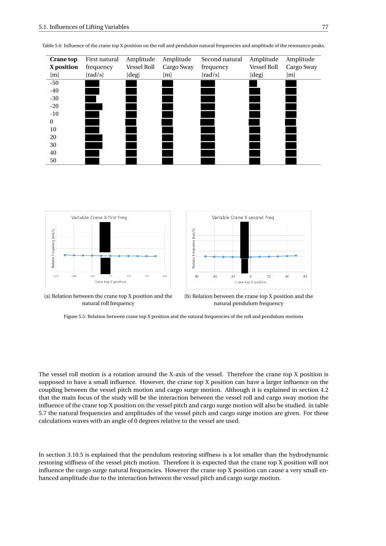
5.1. Influences of Lifting Variables 77
Table 5.6: Influence of the crane top X position on the roll and pendulum natural frequencies and amplitude of the resonance peaks.
Crane topX position
First naturalfrequency
AmplitudeVessel Roll
AmplitudeCargo Sway
Second naturalfrequency
AmplitudeVessel Roll
AmplitudeCargo Sway
[m] [rad/s] [deg] [m] [rad/s] [deg] [m]-50-40-30-20-1001020304050
(a) Relation between the crane top X position and thenatural roll frequency
(b) Relation between the crane top X position and thenatural pendulum frequency
Figure 5.5: Relation between crane top X position and the natural frequencies of the roll and pendulum motions
The vessel roll motion is a rotation around the X-axis of the vessel. Therefore the crane top X position issupposed to have a small influence. However, the crane top X position can have a larger influence on thecoupling between the vessel pitch motion and cargo surge motion. Although it is explained in section 4.2that the main focus of the study will be the interaction between the vessel roll and cargo sway motion theinfluence of the crane top X position on the vessel pitch and cargo surge motion will also be studied. in table5.7 the natural frequencies and amplitudes of the vessel pitch and cargo surge motion are given. For thesecalculations waves with an angle of 0 degrees relative to the vessel are used.
In section 3.10.5 is explained that the pendulum restoring stiffness is a lot smaller than the hydrodynamicrestoring stiffness of the vessel pitch motion. Therefore it is expected that the crane top X position will notinfluence the cargo surge natural frequencies. However the crane top X position can cause a very small en-hanced amplitude due to the interaction between the vessel pitch and cargo surge motion.

78 5. Sensitivity of lifting variables
Table 5.7: Influence of the crane top X position on the cargo surge natural frequency and amplitude of the resonance peak.
Crane topX position
Vessel pitchnaturalfrequency
AmplitudeVessel pitch
AmplitudeCargo Surge
Cargo surgenaturalfrequency
AmplitudeVessel Pitch
AmplitudeCargo Surge
[m] [rad/s] [deg] [m] [rad/s] [deg] [m]-50-40-30-20-1001020304050
5.1.6. Vessel Draught
For the vessel draught two comparisons are made. In the first case a comparison the cargo mass is keptat a percentage of the displacement of the vessel. Thus the cargo mass is dependent on the draught of thevessel. In the second case a comparison the cargo mass is held equal to 3% of the total mass in the multi-bodysystem for a vessel draught of 7 meter. In this way the influence of draught and cargo mass can be studiedmore accurately.
In table 5.8 the comparison of the roll and pendulum natural frequencies with a relative cargo mass is givenfor the first case. In figure 5.6 the natural frequencies of the roll and pendulum motions of the differentdraughts with a relative cargo mass are plotted. In section 3.10.6 is explained that the draught of the vesselinfluences the displacement of the vessel. Via the displacement the mass, added mass and hydrodynamicalstiffness values of the multi-body system are changed. While the hydrodynamic mass matrices are increasedthe cargo weight is also increased since the mass has to stay equal to 3% of the total mass in the system.When the cargo mass stays relative equal to the different displacements there is no change in the natural fre-quencies. This implies that the pendulum restoring stiffness, hydrodynamic stiffness values, hydrodynamicdamping values, added mass values and vessel mass values increase with the same ratio when the draught isincreased.
In table 5.9 the natural frequencies and resonance amplitudes of the vessels roll and pendulum swing motionsare given for different draughts with a constant cargo mass. In figure 5.7 these different natural frequenciesare plotted. Since the weight of the cargo does not change the pendulum restoring stiffness values will alsonot change. Thus only the vessel mass, added mass and hydrodynamical stiffness values change due to theincreased draught. In the table and figure can be seen that the natural frequency changes a little. The in-creased natural frequency for larger draughts shows that the hydrodynamical stiffness values increase morethan the mass and added mass values around the first natural frequencies. Since the cargo mass is relativelighter for larger draughts the influence of the pendulum restoring stiffness values is smaller. This explainsthe reduced natural frequency around the second natural frequency. This is the opposite phenomenon thatoccurs when the cargo mass is increased in section 5.1.1.

5.1. Influences of Lifting Variables 79
Table 5.8: Influence of the vessel draught with relative cargo mass on the roll and pendulum natural frequencies and amplitude of theresonance peaks.
Vessel draughtFirst naturalfrequency
AmplitudeVessel Roll
AmplitudeCargo Sway
Second naturalfrequency
AmplitudeVessel Roll
AmplitudeCargo Sway
[m] [rad/s] [deg] [m] [rad/s] [deg] [m]6.577.588.5
(a) Relation between the vessel draught with a relativecargo mass and the natural roll frequency
(b) Relation between the crane top Y position and thenatural pendulum frequency
Figure 5.6: Relation between the vessel draught with a relative cargo mass and the natural frequencies of the roll and pendulum motions
Table 5.9: Influence of the vessel draught with a constant cargo mass on the roll and pendulum natural frequencies and amplitude ofthe resonance peaks.
Vessel draughtFirst naturalfrequency
AmplitudeVessel Roll
AmplitudeCargo Sway
Second naturalfrequency
AmplitudeVessel Roll
AmplitudeCargo Sway
[m] [rad/s] [deg] [m] [rad/s] [deg] [m]6.577.588.5
(a) Relation between vessel draught with a constant cargomass and the natural roll frequency
(b) Relation between vessel draught with a constant cargomass and the natural pendulum frequency
Figure 5.7: Relation between vessel draught with a constant cargo mass and the natural frequencies of the roll and pendulum motions

80 5. Sensitivity of lifting variables
5.1.7. Metacentric HeightThe metacentric height is varied between 2.5 and 4.5 meters. As explained in section 3.10.7 the metacentricheight has an influence on the stability of the vessel and an increased metacentric height should increasethe natural frequency of the multi-body system. In this section is also explained that the metacentric heightused in the calculations is the metacentric height of the vessel without any cargo in the cranes. A metacentricheight of 2.5 till 4.5 meters might look large but since the cargo is not integrated in the GM values the GMvalues are normal for lifting operations. BigLift shipping uses stability software to calculate the stability ofdifferent loading conditions. The software used for most vessels, including the baseline and case vessel HappySky is called Seasafe. Seasafe shows that a weight of 450 mton will reduce the vessel’s GM from 3.1 meter to1.7 meter. This is a reduction of 1.4 meter due to the weight of the cargo. Larger cargoes will reduce theGM even further. The GM values used in the calculations might look large in comparison with normal GMvalues during lifting operations but the GM values are normal when the cargo mass is not used in the GMcalculations.
In table 5.10 the vessel roll and cargo sway natural frequencies are given as well as the height of the resonancepeaks. In figure 5.8 the vessel roll and cargo sway natural frequencies are plotted with regards to the GM valuesof the vessel. The GM value has a big influence on the roll motions and a smaller influence on the pendulummotions. When the metacentric height is increased the hydrodynamic stiffness matrix will increase whichresults in a higher natural frequency. Since the vessel motions have a higher stiffness and the pendulum iscoupled to the vessel the pendulum natural frequency will also increase. Although to a lesser extent.
Table 5.10: Influence of the vessel’s metacentric height on the vessel roll and cargo sway natural frequency and amplitude of theresonance peak.
GMFirst naturalfrequency
AmplitudeVessel Roll
AmplitudeCargo Sway
Second naturalfrequency
AmplitudeVessel Roll
AmplitudeCargo Sway
[m] [rad/s] [deg] [m] [rad/s] [deg] [m]2.533.544.5
(a) Relation between vessel GM and the natural rollfrequency
(b) Relation between vessel GM and the naturalpendulum frequency
Figure 5.8: Relation between vessel GM and the natural frequencies of the roll and pendulum motions
5.1.8. Results of Lifting Variable Influence StudyThe different variables have a different influence. In table 5.11 the results are summarized. The variable withthe biggest influence is the crane top Z position and crane cable length. This is interesting while the crane topZ position and crane cable length will vary during lifting operations. When a certain crane top crane cablelength is critical for a loading operation one can try to avoid this crane cable length by lowering the crane tipwhich reduces the required crane cable length for the same lifting height or reduce the lifting height itself toavoid a certain crane cable length. At the same time a critical crane top Z position could be worked aroundby changing the crane cable length. Depending on the required lifting height. Therefore it is recommendedto do detailed calculations when the crane top Z position or crane cable length is changed to make sure that

5.1. Influences of Lifting Variables 81
the interaction of both lengths result in a desired natural frequency. The sign of the crane top Y position doesnot change the natural frequency for positive or negative signs, but the peak of the maximum excitation doeschange, which can make port or starboard side lifting more desired. The crane top in X position does notseem to have a significant influence on the different motions. Therefore it is recommended to change othervariables first when the natural frequency of the system must be changed. The displacement of the vesselhas almost no influence on the motions themselves. However the cargo mass will be constant in practice.Therefore a change in draught might reduce the influence of the cargo mass. The exact influence of thedraught and cargo mass together is case sensitive. The metacentric height has a big influence on the vesselroll motions. Therefore it is recommended to do accurate stability studies before critical lifting operationsare performed. The most notable variable is the cargo mass. Since it reduces the first natural frequency andincreases the second natural frequency by a considerable amount. In practice the weight of the cargo cannotbe changed, however the cargo mass varies for every different lifting operation. This shows that it can beuseful to study the multi-body behaviour for all different lifting operations.
The different variables have different influences. Some variables can be changed more easily than othervariables during practice. Therefore it is import to calculate different aspects of a loading operation such aspretension, free hanging and transit of the cargo. With a change of the vessel draught and metacentric heightthe natural frequencies can be changed most safely. The calculations with different Y and X positions of thecrane top can help in the decision of whether the front or aft crane should be used, if the crane should rotateclockwise or counter clockwise to reach it destination and if the lifting operation should be performed fromthe port or starboard side of the vessel when these options are available. The cargo mass can not be changedwhich make the big influence of the cargo weight an interesting value but not useful for the modification ofthe natural frequency.
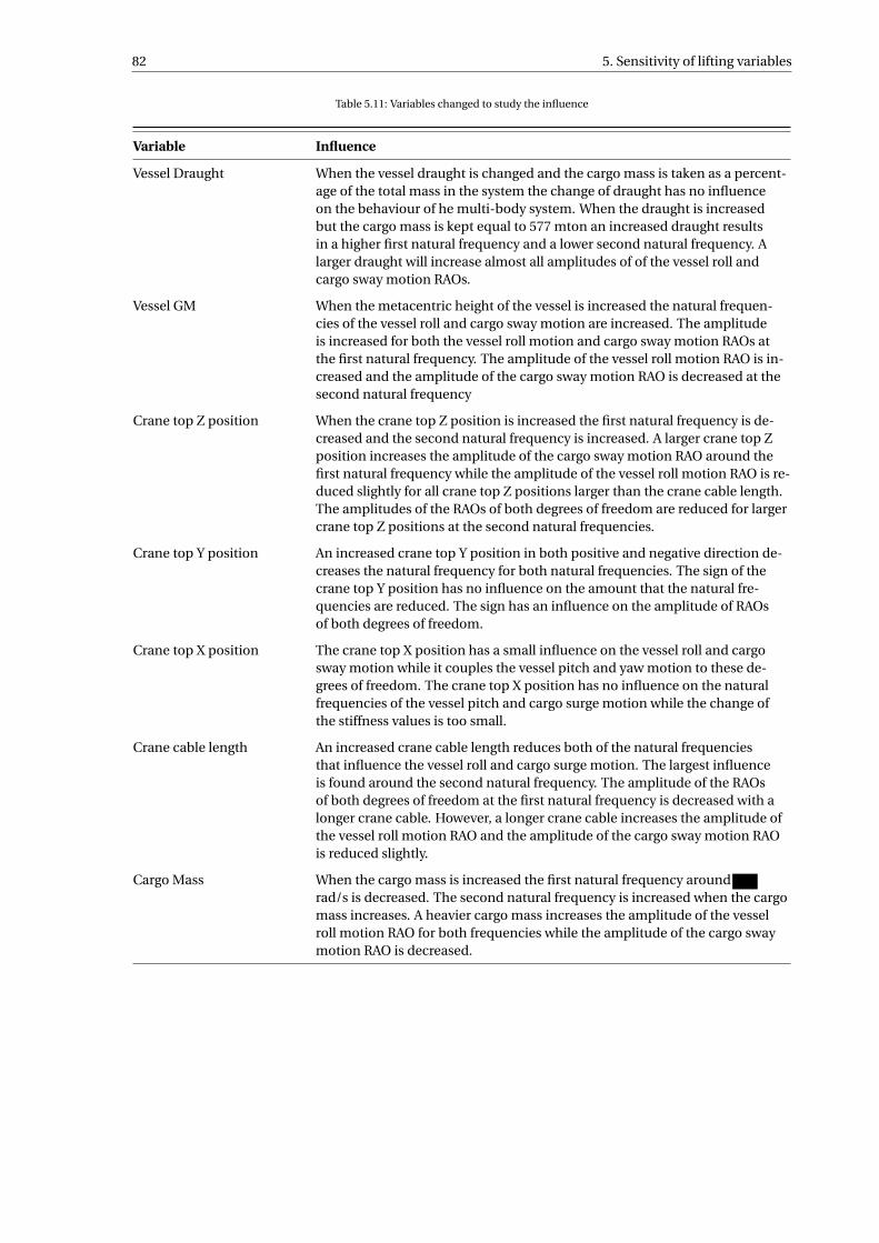
82 5. Sensitivity of lifting variables
Table 5.11: Variables changed to study the influence
Variable Influence
Vessel Draught When the vessel draught is changed and the cargo mass is taken as a percent-age of the total mass in the system the change of draught has no influenceon the behaviour of he multi-body system. When the draught is increasedbut the cargo mass is kept equal to 577 mton an increased draught resultsin a higher first natural frequency and a lower second natural frequency. Alarger draught will increase almost all amplitudes of of the vessel roll andcargo sway motion RAOs.
Vessel GM When the metacentric height of the vessel is increased the natural frequen-cies of the vessel roll and cargo sway motion are increased. The amplitudeis increased for both the vessel roll motion and cargo sway motion RAOs atthe first natural frequency. The amplitude of the vessel roll motion RAO is in-creased and the amplitude of the cargo sway motion RAO is decreased at thesecond natural frequency
Crane top Z position When the crane top Z position is increased the first natural frequency is de-creased and the second natural frequency is increased. A larger crane top Zposition increases the amplitude of the cargo sway motion RAO around thefirst natural frequency while the amplitude of the vessel roll motion RAO is re-duced slightly for all crane top Z positions larger than the crane cable length.The amplitudes of the RAOs of both degrees of freedom are reduced for largercrane top Z positions at the second natural frequencies.
Crane top Y position An increased crane top Y position in both positive and negative direction de-creases the natural frequency for both natural frequencies. The sign of thecrane top Y position has no influence on the amount that the natural fre-quencies are reduced. The sign has an influence on the amplitude of RAOsof both degrees of freedom.
Crane top X position The crane top X position has a small influence on the vessel roll and cargosway motion while it couples the vessel pitch and yaw motion to these de-grees of freedom. The crane top X position has no influence on the naturalfrequencies of the vessel pitch and cargo surge motion while the change ofthe stiffness values is too small.
Crane cable length An increased crane cable length reduces both of the natural frequenciesthat influence the vessel roll and cargo surge motion. The largest influenceis found around the second natural frequency. The amplitude of the RAOsof both degrees of freedom at the first natural frequency is decreased with alonger crane cable. However, a longer crane cable increases the amplitude ofthe vessel roll motion RAO and the amplitude of the cargo sway motion RAOis reduced slightly.
Cargo Mass When the cargo mass is increased the first natural frequency aroundrad/s is decreased. The second natural frequency is increased when the cargomass increases. A heavier cargo mass increases the amplitude of the vesselroll motion RAO for both frequencies while the amplitude of the cargo swaymotion RAO is decreased.

5.2. Influence of Mooring Lines 83
5.2. Influence of Mooring LinesIn section 3.4 is explained that the stiffness of the mooring lines is dependent on the length of the mooringlines. Shorter mooring lines have a higher stiffness value than longer mooring lines. The location of theconnection of the mooring line on shore and on the vessel do determine how the mooring line stiffness isdivided over the X, Y and Z components. In this section multiple mooring line configurations are used tostudy the influence of the mooring lines on the multi-body system.
Multiple mooring configurations are studied. The effects of these configurations will be compared with thebaseline configuration explained in section 4.4. The variables of the lifting configuration are also equal tothe baseline configuration. The first mooring configuration that will be compared is a configuration withtwo mooring lines. Both mooring lines are connected to the stern of the vessel. Since the mooring linesare located at the same side of the vessel the rotational restoring moments will not cancel each other out.The locations of the bollards onshore and fairleads of the vessel can be found in table 5.12. In this table theresulting stiffness components of the mooring lines are also given. Figure 5.9 shows a sketch of the differentmooring lines given in the table. The first configuration consists out of mooring line 1 and mooring line 2 inthis table. The second configuration consists of the first 4 mooring lines from the table. Besides the first twomooring lines two lines at the bow of the vessel will be connected. The stiffness from these mooring lines willadd stiffness in the translations of the vessel. However, the stiffness will have an opposite sign in the vesselpitch and yaw motion in comparison to mooring line 1 and mooring line 2. In the third and last configurationall mooring lines in table 5.12 are used. In this configuration shorter mooring lines are added. In the firstconfiguration only mooring lines at the stern are connected. With this configuration mooring lines will add asmall amount of stiffness in the vessel surge and sway motion. At the same time are rotational restoring forcesintroduced while there is only a negative moment arm in X direction. While this configuration will never beused in practice the configuration can be used mathematically to study the influence of mooring lines at oneside of the vessel. At the second configuration the mooring line stiffness is doubled while 2 more mooringlines with the same length and stiffness values are connected. While these mooring line are connected to thebow of the vessel the rotational forces added in the first configuration are cancelled out by the two new lines.In the third configuration a lot more stiffness than in the first and second configuration are added. Whilemooring lines tend to introduce low amounts of stiffness the influence of stiffer mooring lines are studiedwith the third configuration. This last configuration will not be used in practice but the more extreme valueswill influence the responses of the vessel and cargo in more than the normal configurations.
Table 5.12: Different mooring line configurations used to calculate the influence of mooring lines on the vessel and cargo respones.
Mooringline 1
Mooringline 2
Mooringline 3
Mooringline 4
Mooringline 5
Mooringline 6
Mooringline 7
Mooringline 8
Bollard X [m] -120 -120 120 120 -60 -50 50 60Bollard Y [m] 30 30 30 30 30 30 30 30Bollard Z [m] 5 5 5 5 5 5 5 5Fairlead X [m] -70 -65 65 70 -50 -40 40 50Fairlead Y [m] 10 12 12 10 14 14 14 14Fairlead Z [m] 8 8 8 8 8 8 8 8X stiffness [kN/m] 39.8 38.0 38.0 39.8 63.5 63.5 63.5 63.5Y stiffness [kN/m] 15.9 12.4 12.4 15.9 101.6 101.6 101.6 101.6Z stiffness [kN/m] 2.4 2.1 2.1 2.4 19.1 19.1 19.1 19.1

84 5. Sensitivity of lifting variables
Figure 5.9: Sketch of the mooringline configuration of table 5.12
The different mooring line configurations are used to calculate the responses of the vessel and cargo. As statedbefore the mooring lines will increase the stiffness of the multi body system which will increase the naturalfrequencies of the multi-body system. The repsonses of the vessel roll motion and cargo sway motion areshown in figures 5.10 and 5.11. In these figures can be seen that the first and second mooring configurationsonly have a small influence on the responses of the vessel. The responses of both the vessel roll motion andthe cargo sway motion are increased due to the mooring lines. The third configuration has a larger influenceon the responses of both degrees of freedom. The two natural frequencies that can be seen in these figuresare increased as expected. However the responses of the vessel roll motion and cargo sway motion are in-creased drastically around the first natural frequency. This is also the frequency of swell waves. The changesin response around the second natural frequency are minimal. Therefore it can be stated that the influenceof a stiff mooring configuration has negative influence on the operability of lifting operations.
(a) Vessel roll motion RAO for different mooring lineconfigurations
(b) Vessel roll motion RAO for different mooring lineconfigurations.
Figure 5.10: Influence of different mooring line configurations on the vessel roll motions. The different configurations are combinationsof the lines in table 5.12

5.2. Influence of Mooring Lines 85
(a) Cargo Sway motion RAO for different mooring lineconfigurations
(b) Cargo Sway motion RAO for different mooring lineconfigurations.
Figure 5.11: Influence of different mooring line configurations on the cargo sway motions. The different configurations arecombinations of the lines in table5.12
The eigenvector method is used to study the connection between the different degrees of freedom at thenatural frequency around r ad/s. In figure 5.12 the eigenvector for the vessel and cargo motions withoutmooring lines and the eigenvector for the multi-body system with mooring line configuration 3 are given. Inthis eigenvector graph the vessel roll and cargo sway motion are dominant. Other degrees of freedom are alsoexcited at this natural frequency. Therefore the eigenvector without the vessel roll and cargo sway eigenvectorvalues is plotted in figure 5.13. In figure 5.12 can be seen that the mooring line configuration causes relativelower responses of the vessel roll motion in comparison with the other degrees of freedom. However, thevessel heave motion shows a very small increase of the excitations. Due to the stiffness introduced by themooring lines there is extra stiffness added to the coupling of the vessel heave and roll motions. Due tothese stiffness components energy from the vessel roll motion is transferred to the vessel heave motion whichexplains the small increase of excitation of the vessel heave motion. In figure 5.13 can also be seen thatthe stiffness introduced by the mooring lines in the vessel sway direction prevent the vessel from moving inthis direction. Resulting in a relative smaller excitation of the vessel sway motion at this natural frequency.Other couplings to the vessel surge, cargo surge and cargo heave motion are also introduced. However theinfluence on these degrees of freedom is extremely small. In the equations of motion, found in appendix C,the complete mathematical coupling can be found.

86 5. Sensitivity of lifting variables
Figure 5.12: Eigenvector value comparison between the multi-body system without mooring lines and the multi-body system with astiff mooring line configuration, configuration 3 in figures 5.10 and 5.11. The natural frequency that is compared is the natural
frequency at r ad/s.
Figure 5.13: Eigenvector value comparison between the multi-body system without mooring lines and the multi-body system with astiff mooring line configuration, configuration 3 in figures 5.10 and 5.11. . The natural frequency that is compared is the natural
frequency at r ad/s. In this figure the eigenvector values of the vessel roll and cargo sway motion are neglected
Another aspect that stands out is the small response of the cargo sway motion around r ad/s which canbe seen in figure 5.11. This response is the result of another natural frequency at r ad/s. This naturalfrequency does not influence the vessel roll motion and cargo sway motion with less stiff mooring lines. Theeigenvector method is used to study this natural frequency. In figure 5.14 the eigenvector of this naturalfrequency is shown. This eigenvector makes it clear that the vessel heave and cargo heave motions are thetwo motions with the largest responses on this natural frequency. The stiff mooring line configuration causesa rotational moment due to vessel translations. Due to this phenomenom the vessel heave motion exerts arotational force on the vessel roll and pitch motions. The vessel roll and pitch motions are connected to the

5.2. Influence of Mooring Lines 87
cargo sway and surge motions respectively and this relation causes the excitation of the cargo surge and cargosway motions. A frequency of r ad/s corresponds to a period of seconds. This is a very large periodand will likely not be excited by the swell waves. However, slower waves can still excite this natural frequencyand quadratic drift forces can cause larger motions. These motions are not studied in this research.
Figure 5.14: Eigenvector values of the natural frequency found at r ad/sthat appears when a stiff mooring line configuration isused


6Cargo control systems
As explained in section 2.5 damping might reduce the responses of the cargo motions. Therefore the influenceof damping is modeled and used to study the behaviour of the multi-body system when damping is applied.In section 4.2 is explained that the vessel roll and cargo sway motion show the biggest responses due to waveforces. Therefore the influence of different parameters during the lifting operation was focused on thesetwo degrees of freedom. While the vessel roll and cargo sway motion show the largest responses and arepotentially the most dangerous motions during lifting operations the influence of cargo control systems onthese two degrees of freedom are studied. At those two degrees of freedom the most is gained from reducedresponses.
To create a good understanding of the influence of cargo control systems on the cargo motions the baselinevariables used in section 4.4 will be used. In this way the influence of the different variables are not part ofthe comparison. This means that the crane tip will be placed above the centre of gravity. The vertical locationof the crane tip will be at 30 meters and the distance between the crane tip and cargo centre of gravity will beequal to 20 meters. The mass will be equal to 3 % of the total weight in the multi-body system. The vessel willhave a draught of 7 meters with a metacentric height equal to 3 meters.
In section 6.1 the influence of low stiffness tugger wires and high stiffness tugger wires will be explained.Thereafter the influence of the location of different tugger wires will be described in section 6.2. In section6.3 the influence of passive compensation in terms of small damping percentages will be explained. Next theinfluence of active systems, in terms of large damping values, are explained in section 6.4. All the results aresummarized in section 6.5.
In the equations used to study the influences of the tugger winches two tugger winches are used. The X, Yand Z coordinates of the two tugger winches and padeyes are given in table 6.1. Both winches are mirroredalong the midship line. The X coordinates are placed far away from the cargo and crane tip. This makes itpossible for the crane to move the cargo above the deck. The winches are placed as far as possible the sideof the vessel. This is done to create a large Y component in the damping and spring values from the tuggerwires. In section 6.2 the influence of different configurations will be examined.
Table 6.1: The coordinates of the tugger winches used in the influence calculations of the tugger winch
Coordinate Tugger Winch 1[m] Tugger Winch 2[m]Winch X -30 30Winch Y -15 -15Winch Z 10 10Padeye X -10 10Padeye Y -5 -5Padeye Z -5 -5
89

90 6. Cargo control systems
6.1. Stiffness via tugger winchesIn section 2.5 the influence of damping is explained. In section 3.5 is explained that a cargo control systemwill also introduce stiffness to the multi-body system. In appendix E different methods to control the cargoare described. The damping and mass values of the different types of wires that can be used to control thecargo are neglected in these calculations. The most simple practice to control the cargo is the application offixed tugger winches. These tugger winches will create a connection between the vessel and the cargo with arope or wire. When a fixed tugger system is used the connection will only consist out of a wire and no passiveor active damping is applied. This means that a tugger wire can be modelled as a connection via the restoringforces. The connection can be applied via fibre ropes or steel wires. The only difference between a fibre ropeor steel wire connection in this study is the stiffness of the material. All other aspects of the connection willstay the same for both types of connection. Thus the location of the tugger winch and the connection fromthe tugger wire to the cargo will be on the same locations for both types of lines. To compare the influenceof tugger winches equipped with ropes or wires different stiffness values will be used for the tugger winchcalculations.
In this section the use of polypropylene wires and steel wires connected between the vessel and cargo willbe studied. These wires are connected to the vessel via a tugger winch system that can also pretension thesewires. Therefore these wires are called tugger wires in practice and will be called tugger wires throughout thischapter. The stiffness values of fibre ropes and steel wires differ by 2 to 3 orders of magnitude. Both typesof wires can be used to control the cargo. fibre rope, polypropylene, has stiffness values around 30 kN /mand steel wires kan have a stiffness value of 1000 to 10000 kN /m depending on the diameter of the wires.This large difference in stiffness gives reason to assume different influence on the cargo and vessel motiondepending on the line material. Therefore the influence of both the polypropylene wires and steel wires arestudied. In section 6.1.1 the influence of low-stiffness wires are studied and in section 6.1.2 the influence ofhigh-stiffness tuger wires are studied.
6.1.1. Polypropylene wires
In this section the influence of low-stiffness lines are studied to determine the sensitivity of the motion re-sponses to tugger winches. In this section ’polypropylene’ wires with a stiffness value between 20 kN /m to40 kN /m are studied. In figures 6.1 and 6.2 the RAOs of the vessel roll and cargo sway motion are given for amulti-body system including tugger wires. The lines used in this comparison have an stiffness of 20, 30 or 40kN /m. The stiffness of the lines are low. However, when polypropylene lines are used, the same material asmooring lines, the used stiffness is achievable due to the material properties of polypropylene.
The implementation of the tugger lines will cause a higher stiffness value in the different degrees of free-dom. It is assumed that the weight of the tugger lines is negligible in comparison with the weight of thecargo and the displacement of the vessel. Therefore the tugger lines will not have any influence on the weightof the multi-body system. Since the natural frequency is dependent on the mass and stiffness matrices theincreased stiffness will cause a higher natural frequency. As it was for the baseline calculations and the sen-sitivity calculations done in chapter 4 and chapter 5 the vessel roll and cargo sway motions have two notablenatural frequencies. The other natural frequencies in the system will influence the responses of these twodegrees of freedom in very marginal ways or not at all. The natural frequencies for the tugger line stiffnessvaried between 20 and 40 kN /m are given in table 6.2. In this table the natural frequency is also convertedto the corresponding natural period for easier understanding. The increased stiffness in the system increasesthe first natural frequency from ad/s to r ad/s. While the frequency increases the period of oneharmonic cycle decreases from seconds to seconds. The second natural frequency is increasedfrom r ad/s to r ad/s. Which means that the period is decreased from seconds to seconds.The changes in the natural frequencies are very small while the stiffness added to the system is fairly small.For example the hydrodynamic stiffness of the vessel roll motion is equal to 5.63 ·105kN /m and the restoringstiffness of the pendulum is equal to 2.53 ·105kN /m. The stiffness added to the system on this degree of free-dom due to the tugger winches with a stiffness value of 40 kN /m is equal to 1.27 ·104kN /m. Thus the tuggerwires introduce a stiffness value almost 50 times smaller than the hydrodynamical stiffness of the vessel rollmotion and 20 times smaller of the pendulum restoring stiffness of the cargo in the crane.

6.1. Stiffness via tugger winches 91
(a) Vessel roll motion RAO for a frequency betweenand rad/s for different stiffness values of the tugger
winch
(b) Cargo sway motion RAO for a frequency betweenand rad/s for different stiffness values of the tugger
winch
Figure 6.1: Influence of tugger winches on the vessel roll motion and cargo sway motion RAOs for a frequency between 0.35 and 0.55r ad/s. The stiffness of the tugger ropes is varried between 20 and 40 kN /m.
(a) Vessel roll motion RAO for a frequency betweenand rad/s for different stiffness values of the tugger
winch
(b) Cargo sway motion RAO for a frequency betweenand rad/s for different stiffness values of the tugger
winch
Figure 6.2: Influence of tugger winches on the vessel roll motion and cargo sway motion RAOs for a frequency between 0.65 and 1.05r ad/s. The stiffness of the tugger ropes is varried between 20 and 40 kN /m.
Table 6.2: Natural frequency comparison between different stiffness values of the tugger wire. The first and second natural frequencyare given in radians per second and per second.
Tugger wire stiffess First natural frequency Second natural frequency[kN /m] ω [rad/s] Tn[s] ω [rad/s] Tn[s]No tugger wires connected203040
In figures 6.1 and 6.2 can be seen that the natural frequencies of the multi-body system shift due to the addedstiffness via the tugger wires. The low-stiffness tugger wires do increase the natural frequencies of the multi-body system. Besides increasing the natural frequency the amplitude peak of both the vessel roll and cargosway motion are reduced and with this reduction the range of frequencies at which large responses occur isdecreased. At the second natural frequency the amplitude is increased. This does also increase the frequencyrange at which large responses occur. This change in the RAOs can be explained with the interaction betweenthe vessel and cargo motions. Since no damping is introduced no energy will dissipate from the system. The

92 6. Cargo control systems
connection between the cargo and vessel transfer energy from one body to the other body in the naturalfrequency. Dependent on the natural frequency, phases and excitation forces the equilibrium between cargoand vessel responses will vary for different values in the stiffness, damping and mass matrices. Since thestiffness matrix is changed the equilibrium in responses changes.
The period of the first natural frequency lies between and s. In chapter 1 is explained that theswell waves can be a problem during lifting operations. Swell waves often have a period between the 12 and16 seconds. This means that especially the first natural frequency will be excited by swell waves. To study theinfluence of the different stiffness values on the motions that can occur during lifting operations the mostprobable maximums for the vessel roll and cargo sway motions are calculated. While swell waves are lessrandom than wind waves the frequency and height will vary for each individual wave. At the same time thewind will not increase the wave peaks. Therefore a wave spectra with a peak enhancement factor of 1 willbe used which makes the JONSWAP which is basically a Pierson-Moskowitz spectrum. The significant waveheight is equal to 1 meter in these calculations and the used swell periods are 12, 14 and 16 seconds. In table6.3 the answers of the most probable maximum calculations are given. In figure 6.3 the wave spectra for aperiod of 12, 14 and 16 seconds are plotted. This implies that there is less fluctuation in the wave period fora wave spectrum with a higher period than for a wave spectrum with a lower period. At the same time thereis more energy in the waves with a higher period than the waves with a lower period. More energy in thewaves will mean that the waves will have a larger influence on the vessel and cargo responses when a naturalfrequency occurs at these waves.
The MPM values calculated and showed in table 6.3 are calculated for different wave spectra with a significantwave height of 1 meter. This wave height makes scaling the MPM values extremely easy, while the MPM valuecan be multiplied with the actual wave height of a lifting operation to receive the MPM value of the actuallifting operation. In the tool the significant wave height can be adjusted but for this study the wave heightis taken equal to 1 meter. All MPM values seem very large. However, in reality lifting operations will mostlikely not be performed with wave heights of 1 meter while this causes unsafe operations. For all other MPMcalculations done in this study these same remarks apply.
Figure 6.3: Jonswap spectra for different wave periods. The wave periods are varied between 12 and 16 seconds. The wave height is setto 1 meter and the peak enhancement factor is equal to 1.
In figures 6.4 and 6.5 the response spectra for different tugger wires with different wave spectra are given.These response spectra do explain how the multi-body system does react to specific wave spectra. The re-sponse spectra are also used to calculate the most probable maximum values of the different tugger wireconfigurations and different wave spectra. The figure shows that the different wave spectra can influence theheight of the responses. For example, the green line in figure 6.4 shows that the wave spectra for a period of14 seconds generate larger responses from both the vessel roll motion and the cargo sway motion than theother wave spectra do for the different stiffness values. Figure 6.5 shows that the second natural frequencyhas a larger influence on the response of the cargo sway motion than on the vessel roll motion.

6.1. Stiffness via tugger winches 93
(a) Vessel roll motion RAO for a frequency betweenand rad/s for different stiffness values of the tugger
winch
(b) Cargo sway motion RAO for a frequency betweenand rad/s for different stiffness values of the tugger
winch
Figure 6.4: Influence of tugger winches on the vessel roll motion and cargo sway motion RAOs for a frequency between andr ad/s. The stiffness of the tugger ropes is varried between 20 and 40 kN /m.
(a) Vessel roll motion RAO for a frequency betweenand rad/s for different stiffness values of the tugger
winch
(b) Cargo sway motion RAO for a frequency betweenand rad/s for different stiffness values of the tugger
winch
Figure 6.5: Influence of tugger winches on the vessel roll motion and cargo sway motion RAOs for a frequency between andr ad/s. The stiffness of the tugger ropes is varried between 20 and 40 kN /m.
When tugger wires are connected the stiffness of the multi-body system increases. In table 6.2 is showed thattugger wires with a stiffness value of 40 kN /m reduce the natural frequency to a maximum period ofseconds. This shift of the natural period towards the 12 seconds and the decreased response of the vesselroll motion will both influence the MPM of the vessel roll motion. The MPMs for the different tugger wirestiffness values and wave spectra are given in table 6.3. The increased natural frequency will result in higherMPM values for the vessel roll motion for waves with a period of 14 seconds than waves with a higher or lowerperiod. This can already be achieved with tugger wires with a stiffness of 20 kN /m. Since the influence ofthe second natural frequency was already large on the cargo sway motions, as explained in section 4.4, theincreased natural frequencies will only enhance this effect which results in even higher MPM for the cargosway motion for waves with a period of 12 seconds. The MPM of the cargo sway motions stay around equalfor waves with a period of 14 seconds and is even reduced for waves with a period of 16 seconds.

94 6. Cargo control systems
Table 6.3: Most probable maximum comparison between different stiffness values of the tugger wire. The MPMs are calculated for swellwaves with a period of 12, 14 and 16 seconds.
Tugger damping MPM Tp = 12 MPM Tp = 14 s MPM Tp = 16 s
[kN /m]VesselRoll
CargoSway
VesselRoll
CargoSway
VesselRoll
CargoSway
No tuggerwires connected203040
6.1.2. Steel wiresBeside low-stiffness fibre rope tugger wires steel tugger wires can be used to control the cargo. Steel tuggerwires have a higher stiffness value for the same diameter of the wire than fibre rope wires. When steel tuggerwires are used with a diameter between 0.035 and 0.055 meter stiffness values between 4000 kN /m and 10000 kN /m can be achieved in this winch configuration. A wire with a diameter of 5.5 centimeter is extremelylarge for tugger wires. However the large stiffness values they introduce are intresting to study. Tugger wireswith these stiffness values will almost create a rigid connection between the vessel and cargo. This increasedstiffness will have a much larger influence on the multi-body stiffness than the tugger wires with a relativelylow stiffness. In figure 6.7 the RAOs of the vessel roll motion are given for a multi-body system includingtugger wires. The wires used in this comparison have an stiffness of 4000, 6000, 8000 or 10000 kN /m. Figure6.8 shows the RAOs of the cargo sway motion in the same conditions.
The first thing that stands out are the small RAO values of the cargo roll motion. Especially for frequenciesbetween r ad/s and ad/s the responses are small. However, these RAO of the cargo sway motionsbecome extremely large at this frequency. Especially for wire stiffness values equal to 4000 kN /m and 6000kN /m. Instead of a small frequency range in which a larger amplitude can be seen the multi-body systemshow large RAO values for wave frequencies between 0.15 and 0.55 r ad/s. At frequencies between r ad/sand ad/s the complete opposite occurs. At these higher frequencies shown in figure 6.8 the vessel rollmotion shows behaviour that would show that natural frequencies occur here. However these natural fre-quencies do not show at the responses of the cargo sway motions. Instead of resonance peaks the cargo swaymotion show anti-resonance peaks. To understand the natural frequencies tot occur between r ad/s and
r ad/s the natural frequencies are studied with the eigenvector method. The natural frequencies of thedifferent tugger wire stiffness values are given in table 6.4. The eigenvector is shown in figure 6.6. In thisfigure can be seen that at this natural frequency the cargo roll motion has the largest response of all degreesof freedom. The stiff tugger wires connect the cargo roll motion to the vessel roll motion and cargo sway mo-tion. However, the responses of the cargo sway motion are lower at the natural frequency than at frequenciesaround this natural frequency. Another aspect that can be learned from this eigenvector study is the influenceof stiff tugger wires on the cargo roll motion. These stiff tugger wires forces the cargo into a rolling motion.This motion can be dangerous during lifting operations. Especially for cargoes with large sizes. Due to someof the simplifications not all moments that act on the cargo body are applied in the model. In reality therotations of the cargo body can be smaller than the eigenvector shows in figure 6.6.

6.1. Stiffness via tugger winches 95
Figure 6.6: Eigenvector of the natural frequency that occurs when steeltugger wires are used. The natural frequency can be seen infigure 6.8a
Even though there are natural frequencies between r ad/s and r ad/s the responses of the two bodiesmight be reduced in comparison with the multibody system without tugger winches. Therefore the mostprobable maximum for the vessel roll and cargo sway motions are calculated. In table 6.5 the MPMs areshown for all different stiffness values and wave periods used. The wave periods are taken equal to the periodsused in section 6.1.1. In this table is shown that most of the most probable maximum values for the vessel rollmotion are lower when stiff tugger wires are used. Especially the tugger wire stiffness of 10000kN /m reducesthe most probable maximum a lot. The cargo sway motion has a larger MPM for stiffness values between4000 kN /m and 6000 kN /m. The MPM of the cargo sway motion is smaller for stiffness values between 8000kN /m and 10000kN /m. However, these stiff tugger wires should not be used. The vessel roll motion andcargo sway motions might show a reduction in their most probable maximum the large response of the cargoroll motion can be dangerous.
(a) Vessel roll motion RAO for a frequency betweenand r ad/s for different stiffness values of the tugger
winch
(b) Cargo sway motion RAO for a frequency betweenand r ad/s for different stiffness values of the tugger
winch
Figure 6.7: Influence of tugger winches on the vessel roll motion and cargo sway motion RAO for a frequency between andr ad/s. The stiffness of the tugger ropes is varried between 4000 and 10000 kN /m.

96 6. Cargo control systems
(a) Vessel roll motion RAO for a frequency betweenand rad/s for different stiffness values of the tugger
winch
(b) Cargo sway motion RAO for a frequency betweenand rad/s for different stiffness values of the tugger
winch
Figure 6.8: Influence of tugger winches on the vessel roll motion and cargo sway motion RAO for a frequency between andr ad/s. The stiffness of the tugger ropes is varried between 4000 and 10000 kN /m.
Table 6.4: Natural frequency comparison between different stiffness values of the tugger wire.
Tugger wire stiffness Natural frequency[kN /m] ω [rad/s] Tp [s]40006000800010 000
Table 6.5: Most probable maximum comparison between different stiffness values of the tugger wire. The MPMs are calculated for swellwaves with a period of 12, 14 and 16 seconds.
Tugger wire stiffess MPM Tp = 12 [s] MPM Tp = 14 [s] MPM Tp = 16 [s]
[kN]VesselRoll
CargoSway
VesselRoll
CargoSway
VesselRoll
CargoSway
No tuggerwires connected40006000800010000
Extremely stiff connections can result in rigid connections. In figure 6.9 the RAOs of the vessel sway motionare plotted for different tugger wire stiffness values. These figures show that the cargo sway and vessel swaymotion are not coupled in such a way that they influence each other. What can be seen is that the smallcoupling to the vessel roll and cargo sway motion does not occur when the cargo and vessel are connectedwith stiff tugger wires. The stiff tugger wires will reduce the amount of energy transferred from the vessel rollmotion and cargo sway motion to the vessel sway motion around this natural frequency.

6.2. Location of tugger winches 97
(a) Vessel sway motion RAO for a frequency betweenand rad/s for different stiffness values of the tugger
winch
(b) Vessel sway motion RAO for a frequency betweenand rad/s for different stiffness values of the tugger
winch
Figure 6.9: Influence of tugger winches on the vessel roll motion and cargo sway motion RAO for a frequency between andr ad/s. The stiffness of the tugger ropes is varried between 4000 and 10000 kN /m.
6.2. Location of tugger winchesIn section 6.1 is explained how tugger winches with a low stiffness and tugger winches with a large stiffnessvalue influence the vessel and cargo responses. The configuration of the tugger winches are kept constantin these cases. However, a change in the configuration can show interesting changes in the responses of thevessel and cargo motions. Therefore multiple configurations are studied. In section 3.5 is explained that thestiffness and damping coefficients for every direction are dependent on the length ratio between the lengthof in a specific direction and total length of the tugger wire. When the configuration is changed the stiffnesscomponents of the tugger wires will change. These stiffness values will influence the responses of the vesseland cargo responses.
Three different tugger winch configurations are compared. The configurations used to study the influencesare given in table 6.6. In this table the location of the connection to the cargo is given by the padeye value. Allthe three different configurations will consist of two tugger winches and the tugger wires will have a stiffnessvalue of 30 kN /m. Since the same amount of tugger winches are used the total added stiffness in the multi-body system will stay the same. The first configuration is the same configuration that is used in section 6.1.In this configuration the tugger winches have a relatively large X-component. This results in relatively largestiffness values in X-direction. For this reason the second configuration has been chosen so that there isno distance in X direction between the tugger winch and the connection with the load. This increases thestiffness components in Y and Z direction. These two stiffness components will influence the vessel roll andcargo sway motions the most. In the third configuration the winches are located at opposite sides in X and Ydirection. Since the two winches will apply opposite rotational moments in certain directions the influenceon the rotations off both the vessel and cargo will change.
Table 6.6: Three different tugger winch configurations used to calculate the influence of the tugger winch configuration.
Coordinate Configuration 1 Configuration 2 Configuration 3TuggerWinch 1
TuggerWinch 2
TuggerWinch 1
TuggerWinch 2
TuggerWinch 1
TuggerWinch2
Winch X [m] -30 30 -10 10 -30 30Winch Y [m] -15 -15 -15 -15 -15 15Winch Z [m] 10 10 10 10 10 10Padeye X [m] -10 10 -10 10 -10 10Padeye Y [m] -5 -5 -5 -5 -5 5Padeye Z [m] -5 -5 -5 -5 -5 -5X stiffness [kN/m] 22.2 22.2 0.0 0.0 22.2 22.2Y stiffness [kN/m] 11.1 11.1 16.6 16.6 11.1 11.1Z stiffness [kN/m] 16.7 16.7 25.0 25.0 16.7 16.7

98 6. Cargo control systems
In configuration 2 the X component of the stiffness value is reduced. While the stiffness of the complete tug-ger line stays equal to the stiffness value in configuration the stiffness components in Y and Z direction willincrease. The stiffness component in X direction does not influence the vessel roll and cargo sway motion.The roll motion is influenced by both the stiffness components in Y and Z direction and the cargo sway mo-tion is only influenced by the stiffness components in Y direction. This means that the stiffness componentsthat are import for the natural frequency of the combined vessel roll and cargo sway motion increases. Theincreased stiffness values will cause higher natural frequencies. This can be seen in figures 6.10 and 6.11. Thenatural frequencies of all different tugger winch configurations are given in table 6.7.
In configuration 3 the X and Y locations of the two winches and connections to the cargo are mirrored. Sincethe X, Y and Z components of the tugger wire will have the same length as in configuration 1 the stiffnesscomponents in these directions will have the same value as in configuration 1. However, the rotational mo-ments and restoring forces due to rotations of the two bodies are dependent on the location of the winch andlocation of the connection to the cargo. Since these locations are in opposite direction for both winches therotational moments transferred via the two tugger wires will cancel each other for some degrees of freedom.However some other relations that where cancelled in the first configuration occur in configuration 3. Themost notable change is the relation between the vessel roll and vessel pitch motion. In the first configurationthis relation was cancelled but in the third configuration there are large stiffness values between these twodegrees of freedom. The vessel pitch and vessel yaw motion are also coupled via the tugger wires in the thirdconfiguration while this connection was cancelled in the first configuration. This influence will be studiedlater in this section. The stiffness components between the vessel roll and cargo sway motion do also differbetween the first and third configuration. The stiffness components between these two degrees of freedomare smaller in the third configuration which will reduce the stiffness in the multi-body system and reducethe natural frequency. This can be seen in figures 6.10 and 6.11. This tugger wire configuration reduces theresponses of the vessel and cargo motions. This can also be seen in the figures.
As stated earlier the third tugger winch configuration introduces larger stiffness values to the vessel pitch andcargo sway motion. To study the influence of the tugger winch configuration on the vessel pitch and cargosurge motion the RAOs of these degrees of freedom are shown in figures 6.12 and 6.13. In these figures canbe seen that the cargo surge motion is extremely large for frequencies between r ad/s and r ad/s.In this range of frequencies two natural frequencies are shown. one at r ad/s and one at r ad/s.The natural frequency of r ad/s is the same natural frequency that occurs in the vessel roll and cargosway motion. This shows that the third tugger winch configuration couples these vessel roll and cargo swaymotions to the vessel pitch and cargo surge motion. This can also be seen in the eigenvector given in figure6.15. The natural frequency at r ad/s is the natural frequency of the cargo surge motion This motion isalready studied in section 4.2. However due to the coupling between the vessel roll motion and cargo swaymotion the cargo surge motion receives energy from waves with a direction of 90 degrees and the naturalfrequency of this degree of freedom gets excited. The eigenvector of the natural frequency of r ad/s isshown in figure 6.14. This figure shows that the cargo surge motion also transfers energy to the vessel roll andcargo sway motion. This explains the new natural frequency that can be seen in figures 6.10b and 6.11b. Theexcitations of the vessel roll motion and cargo sway motion is also proof that tugger winch configuration 3couples the cargo surge to the cargo sway and vessel roll motions.

6.2. Location of tugger winches 99
(a) Vessel roll motion RAO for a frequency betweenand rad/s for different stiffness values of the tugger
winch
(b) Vessel roll motion RAO for a frequency betweenand rad/s for different stiffness values of the tugger
winch
Figure 6.10: Influence of the tugger winch configuration on the vessel roll motion RAO. Configurations of the tugger winches are givenin table 6.6
(a) Cargo sway motion RAO for a frequency betweenand rad/s for different stiffness values of the tugger
winch
(b) Cargo sway motion RAO for a frequency betweenand rad/s for different stiffness values of the tugger
winch
Figure 6.11: Influence of the tugger winch configuration on the cargo sway motion RAO. Configurations of the tugger winches are givenin table 6.6
(a) Vessel pitch motion RAO for a frequency betweenand rad/s for different stiffness values of the tugger
winch
(b) Vessel pitch motion RAO for a frequency betweenand rad/s for different stiffness values of the tugger
winch
Figure 6.12: Influence of the tugger winch configuration on the vessel pitch motion RAO. Configurations of the tugger winches are givenin table 6.6
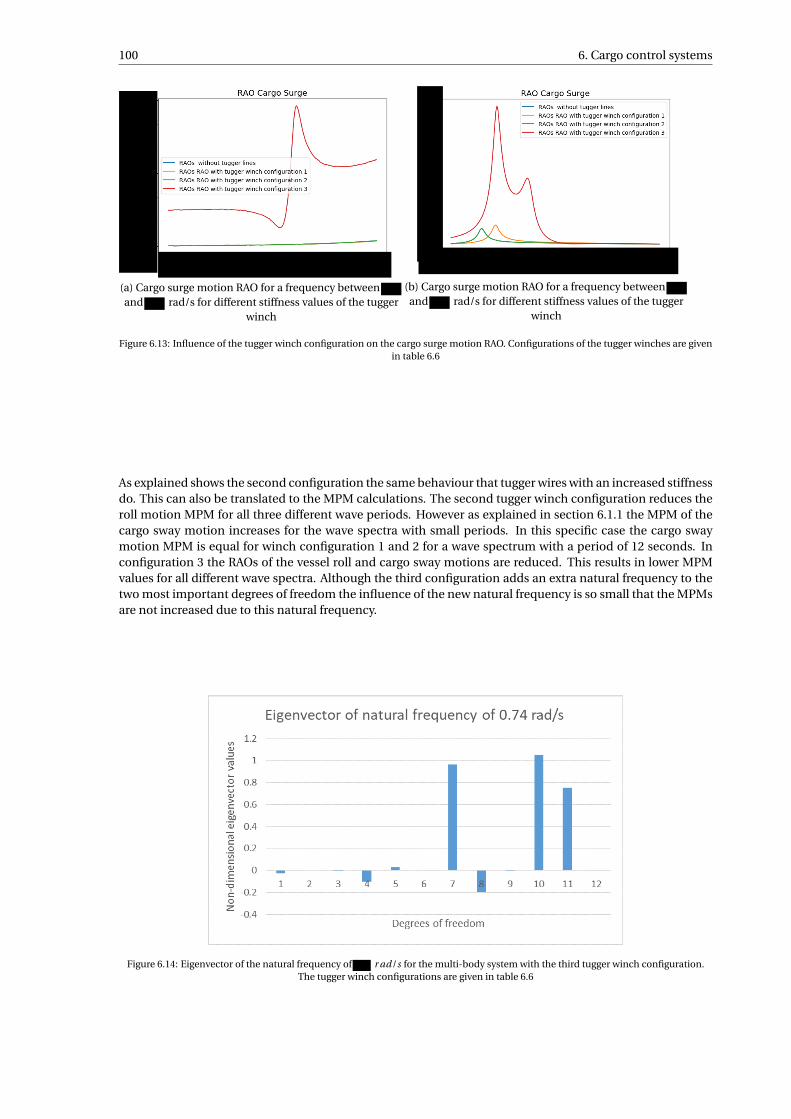
100 6. Cargo control systems
(a) Cargo surge motion RAO for a frequency betweenand rad/s for different stiffness values of the tugger
winch
(b) Cargo surge motion RAO for a frequency betweenand rad/s for different stiffness values of the tugger
winch
Figure 6.13: Influence of the tugger winch configuration on the cargo surge motion RAO. Configurations of the tugger winches are givenin table 6.6
As explained shows the second configuration the same behaviour that tugger wires with an increased stiffnessdo. This can also be translated to the MPM calculations. The second tugger winch configuration reduces theroll motion MPM for all three different wave periods. However as explained in section 6.1.1 the MPM of thecargo sway motion increases for the wave spectra with small periods. In this specific case the cargo swaymotion MPM is equal for winch configuration 1 and 2 for a wave spectrum with a period of 12 seconds. Inconfiguration 3 the RAOs of the vessel roll and cargo sway motions are reduced. This results in lower MPMvalues for all different wave spectra. Although the third configuration adds an extra natural frequency to thetwo most important degrees of freedom the influence of the new natural frequency is so small that the MPMsare not increased due to this natural frequency.
Figure 6.14: Eigenvector of the natural frequency of r ad/s for the multi-body system with the third tugger winch configuration.The tugger winch configurations are given in table 6.6

6.3. Passive compensation 101
Figure 6.15: Eigenvector of the natural frequency of r ad/s for the multi-body system with the third tugger winch configuration.The tugger winch configurations are given in table 6.6
Table 6.7: Natural frequency comparison between different stiffness values of the tugger wire. The first and second natural frequencyare given in radians per second and per second.
Tugger winch configuration First natural frequency Second natural frequency[kN /m] ω [rad/s] Tn[s] ω [rad/s] Tn[s]No tugger wires connectedConfiguration 1Configuration 2Configuration 3
Table 6.8: Most probable maximum comparison between different tugger winch configurations. The tugger winch configurations canbe found in table 6.6. The MPMs are calculated for swell waves with a period of 12, 14 and 16 seconds.
Tugger Winch Configuration MPM Tp = 12 MPM Tp = 14 s MPM Tp = 16 s[kN /m] Roll Sway Roll Sway Roll SwayNo tuggerwires connectedConfiguration 1Configuration 2Configuration 3
6.3. Passive compensationNow that the influence of tugger wires with a small and large stiffness component are known damping can beadded to the system. The least complex way to implement damping is via a passive system. In section 2.5 andappendix E is explained that constant tension tugger winches are reactive to the relative motions between thecargo and the vessel. Due to the reactive behaviour the tension is adjusted after a fluctuation in the tensionoccurs. Over the extend of a full harmonic oscillation damping is applied to the multi-body system. However,it is difficult to impossible to determine the amount of damping that will be applied to the system via constanttension tugger winches. Another way to apply damping is via a system that is related to the passive heavecompensation modules. Via hydraulics or pneumatics damping is added to the system. However, it is alsoimpossible to determine the damping for such a system and developing a passive damping module is notpart of this thesis. Reducing the motions is part of the thesis. Therefore it is assumed that damping can beadded to the system in a passive way. Since there are multiple examples given to apply passive damping thisis an accurate assumption.

102 6. Cargo control systems
Since the exact amount of damping can not be calculated for passive compensation systems it is assumedthat the passive compensators will apply a percentage of the critical damping. The critical damping will becalculated for the stiffness applied via the tugger wires and the mass of the cargo. Since passive dampingis not the most optimal form of damping it is assumed that the amount of damping will be equal to 5% to15% of the critical damping. While the stiff tugger winches do not show any natural frequencies close to theswell wave periods the passive compensation is applied to the less stiff tugger wires used in section 6.1.1.Therefore the stiffness of the tugger wire is equal to 30 kN /m in this section. In figures 6.16 and 6.17 theRAOs are given for the vessel roll motion and cargo sway motion with damping applied. In figures 6.16a and6.17a can be seen that the damping reduces the responses at the natural frequencies significantly. However,these figures do also show that damping also broadens the amplitude of the response around the naturalfrequency. However the extent to which the response spectra is broaden is negligible. Since the amount ofapplied damping is relatively small the natural frequency should not be influenced by the damping. This canbe seen in the figures and also in table 6.9.
(a) Vessel roll motion RAO for a frequency betweenand rad/s for different damping values of the tugger
winch
(b) Vessel roll motion RAO for a frequency betweenand rad/s for different damping values of the tugger
winch
Figure 6.16: Influence of damping applied via tugger winches on the vessel roll motion RAO. The damping of the tugger ropes is variedbetween 5% and 15% of ξ.
(a) Cargo sway motion RAO for a frequency betweenand rad/s for different damping values of the tugger
winch
(b) Cargo sway motion RAO for a frequency betweenand rad/s for different damping values of the tugger
winch
Figure 6.17: Influence of damping applied via tugger winches on the cargo sway motion RAO. The damping of the tugger ropes is variedbetween 5% and 15% of ξ.

6.3. Passive compensation 103
Table 6.9: Natural frequency comparison between different dampin values of the tugger wire. The tugger wire stiffness used in thecalculations is 30 kN. The MPMs are calculated for swell waves with a period of 12, 14 and 16 seconds.
Tugger damping First natural frequency Second natural frequencyω [rad/s] Tp [s] ω [rad/s] Tp [s]
No damping applied0.05%0.1%0.15%
In tables 6.10 till 6.12 the most probable maximum can be found for the same three different wave periods asused in the previous sections and the three different damping percentages. The reduction of the responsesdue to damping influence the MPM calculations. The more damping is applied damping the greater thereduction of the most probable maximum for all different wave periods. In this multi-body system damp-ing does exactly what we expect. As explained in section 6.1.1, the natural frequencies are located withinthe energy density distribution of the wave spectra. Since damping has the most influence on the naturalfrequencies the damping will reduce the vessel and cargo responses. However between the two natural fre-quencies of the cargo sway motion there is a fairly high response for the cargo sway motion. Between and
r ad/s the cargo sway motion has a response of meters. Damping is not effective at influencing thisresponse. Which explains the high MPM values of the cargo sway motion.
Tables 6.10 till 6.12 also show the reduction of the vessel roll motion MPM and cargo sway motion MPMrelative to the MPM of these two degrees of freedom where no tugger wires are applied to the multi-bodysystem. In the tables can be seen that small amounts of damping have a relatively large influence on thereduction of the MPMs. For all three different wave periods the reduction of the MPM due to damping has thesame order size. However, larger amounts of damping have a relatively larger influence for MPMs for a periodof 12 seconds. In figures 6.16 and 6.17 can be seen that damping has the largest influence on the naturalfrequency around r ad/s. While wave spectra with a period of 12 seconds have a larger influence onthis natural frequency than wave spectra with a larger period the influence of damping is larger on the MPMsis larger for this period. Besides the small differences between the different wave spectra periods it can bestated that damping has a positive effect on reducing both the vessel roll and cargo sway motion.
Table 6.10: Most probable maximum comparison between different critical damping values of the tugger wire. The tugger wire has astiffness of 30 kN. The MPMs are calculated for swell waves with a period of 12 seconds.
Tugger Damping MPM Tp = 12Vessel Roll Cargo Sway[deg] reduction [deg] reduction
No tugger winchStiffness 30 kN/m, No DampingStiffness 30 kN/m, Damping = 0.05ξcr i t
Stiffness 30 kN/m, Damping = 0.10ξcr i t
Stiffness 30 kN/m, Damping = 0.15ξcr i t
Table 6.11: Most probable maximum comparison between different critical damping values of the tugger wire. The tugger wire has astiffness of 30 kN. The MPMs are calculated for swell waves with a period of 14 seconds.
Tugger Damping MPM Tp = 14Vessel Roll Cargo Sway[deg] reduction [deg] reduction
No tugger winchStiffness 30 kN/m, No DampingStiffness 30 kN/m, Damping = 0.05ξcr i t
Stiffness 30 kN/m, Damping = 0.10ξcr i t
Stiffness 30 kN/m, Damping = 0.15ξcr i t

104 6. Cargo control systems
Table 6.12: Most probable maximum comparison between different critical damping values of the tugger wire. The tugger wire has astiffness of 30 kN. The MPMs are calculated for swell waves with a period of 16 seconds.
Tugger Damping MPM Tp = 16Vessel Roll Cargo Sway[deg] reduction [deg] reduction
No tugger winchStiffness 30 kN/m, No DampingStiffness 30 kN/m, Damping = 0.05ξcr i t
Stiffness 30 kN/m, Damping = 0.10ξcr i t
Stiffness 30 kN/m, Damping = 0.15ξcr i t
6.4. Active damping
Another way to apply damping is via an active system. In an active system damping will be applied by a winchas explained in section 2.5 and appendix E. In an active system the applied damping follows from the speedthat the controller acts and the limitations of the winch. Since it is not the purpose of this research to developactive tugger winches the dimensions and limitations are unknown. However, a research from Heerema Ma-rine Contractors [19] shows that there are tugger winches with a capacity of more than 600 kN /m/s. Whenthe critcal damping equation given in equation 3.14 is used for tugger winches with a stiffness of 30 kN /m itshows that the critical damping is equal to kN /m/s when the critical damping is calculated with the tug-ger wire stiffness and mass of the cargo. This means that the critical damping is lower than the damping thatcan be applied with active tugger winches. Therefore the active winch configuration will be used to calculatethe influence of high damping values.
In section 6.1 it became clear that stiff tugger winches will increase the natural frequencies by such a largevalue that the two important natural frequencies of the multi-body system are almost not excited by thewaves with a period of 12 to 16 seconds. However, the response of the roll motion between these two naturalfrequencies where quite large. The response of the roll motion is not influenced by the damping. Thereforethe less stiff tugger wires are used in the active tugger winch configuration. The influence of tugger wireswith a stiffness of 30 kN /m in combination with a damping of 100, 200, 300 and 400 kN /m/s are plotted infigures 6.18 and 6.19. The damping values of 100, 200 and 300 kN /m/s are smaller than the critical damping.Therefore they should reduce the responses of the vessel and cargo motions. The damping values of 400kN /m/s is larger than the critical damping value. The over damped system causes a slower return to theequilibrium positions of the vessel and cargo bodies after an excitation. This is explained in section 2.5 andcan be seen in figure 2.8. However, the stiffness of the multi-body system is not only dependent on the tuggerwires. The restoring stiffness of the coupling of the cargo via the crane cables and the vessel hydrodynamicrestoring stiffness are also a large part of the stiffness values. While these stiffness values are not taken intoaccount for the critical damping calculation the damping will not be equal to the critical damping of themulti-body system.
In figures 6.18 and 6.19 can be seen that damping reduces the amplitude of the RAOs. However, damping doesalso increase the width of the response spectra. This phenomenom is extremely clear in figures 6.18a and6.19a. While waves will not occur in a single frequency but in a wave spectra as explained in section 2.2 thiswider response spectra might increase the most probable maximum when damping is increased. Thereforethe response spectra of the vessel roll motion and cargo sway motion are given in figures 6.20 and 6.21. Whenthe energy density function of a wave spectrum lies outside but close to the natural frequency of a degree offreedom the MPMs might increase. The response spectra show that the increased damping results in smallerresponse peaks but a larger response range. However, the amplitude peak is reduced so much that all thelarger range of responses should not increase the MPMs. In the figures can also be seen that damping largerthan the critical damping values will decrease the amplitude of the responses while the critical damping ofthe combined stiffness values in the degrees of freedom are not exceeded.

6.4. Active damping 105
(a) Vessel roll motion RAO for a frequency betweenand rad/s for different damping values of the tugger
winch
(b) Vessel roll motion RAO for a frequency betweenand rad/s for different damping values of the tugger
winch
Figure 6.18: Influence of damping applied via tugger winches on the vessel roll motion RAO. The stiffness of the tugger wires is set to30kN /m and the damping is varied between 100 and 400 kN /m/s
(a) Cargo sway motion RAO for a frequency betweenand rad/s for different damping values of the tugger
winch
(b) Cargo sway motion RAO for a frequency betweenand rad/s for different damping values of the tugger
winch
Figure 6.19: Influence of damping applied via tugger winches on the cargo sway motion RAO. The stiffness of the tugger wires is set to30kN /m and the damping is varied between 10 and 30 kN /m/s

106 6. Cargo control systems
(a) Vessel roll motion response for a frequency betweenand rad/s for different damping values of the
tugger winch. The wave spectra used is a Jonswap spectrawith Tp = 14 s and γ = 1.0
(b) Vessel roll motion response for a frequency betweenand rad/s for different damping values of the
tugger winch. The wave spectra used is a Jonswap spectrawith Tp = 14 s and γ = 1.0
Figure 6.20: Influence of damping applied via tugger winches on the vessel roll motion response spectra. The stiffness of the tuggerwires is set to 30kN /m and the damping is varied between 100 and 400 kN /m/s. The wave spectra used is a Jonswap spectra with Tp =
14 s and γ = 1.0
(a) Cargo sway motion response for a frequency betweenand rad/s for different damping values of the
tugger winch. The wave spectra used is a Jonswap spectrawith Tp = 14 s and γ = 1.0
(b) Cargo sway motion response for a frequency betweenand rad/s for different damping values of the
tugger winch. The wave spectra used is a Jonswap spectrawith Tp = 14 s and γ = 1.0
Figure 6.21: Influence of damping applied via tugger winches on the cargo sway motion response spectra. The stiffness of the tuggerwires is set to 30kN /m and the damping is varied between 100 and 400 kN /m/s. The wave spectra used is a Jonswap spectra with Tp =
14 s and γ = 1.0
In tables 6.13 till 6.15 the most probable maximum values calculated with the multi-body tool with applieddamping values of 100, 200, 300 and 400 kN /m/s. In the tables wave spectra with a period of 12, 14 and 16seconds are used to calcualte the MPM values. The reduction relative to the MPM of the multi-body systemwithout tugger wires is also shown. In the tables can be seen that the difference in reduction due to differentdamping values is relatively small. The tables show that a damping value of 400 kN /m/s has a smaller influ-ence on the most probable maximum than a damping a damping value of 300 kN /m/s for all different wavespectra periods.
Tugger wires with a damping value of 300 kN /m/s show the largest reduction of the MPM values for both thevessel roll and cargo sway motions. As explained in section 6.3 the natural frequency around r ad/s isreduced more than the natural frequency around r ad/s. This also applies for large amounts of damp-ing, hence the MPMs for a wave spectra with a period closer to this natural frequency show a larger reduction.

6.4. Active damping 107
For the wave spectra with a period of 12 seconds the difference between 100 kN /m/s damping and 300kN /m/s is the influence of an increased amount of damping the largest. For all other wave spectra peri-ods the increased reduction due to larger damping values is relatively smaller. The vessel roll motion MPMhas a reduction of 41.9 % for damping values equal to 100 kN /m/s and a reduction of % for dampingvalues equal to 300 kN /m/s. Thus 200 kN /m/s extra damping increases the reduction of the MPM valuewith only %. For the cargo sway motion and all other wave spectra periods the increased reduction is evensmaller. This shows that small amounts of damping have a relatively large influence on the MPM values ofthe multi-body system. This was also a result given in section 6.3.
Table 6.13: Most probable maximum comparison between different damping values and a stiffness value of 30 kN /m. The damping hasbeen varied between 100 kN /m/s and 400 kN /m/s. The swell waves have a period of 12 seconds.
Tugger Damping MPM Tp = 12Vessel Roll Cargo Sway[deg] reduction [deg] reduction
No tugger winchStiffness 30 kN/m, No DampingStiffness 30 kN/m, Damping = 100 kN/m/sStiffness 30 kN/m, Damping = 200 kN/m/sStiffness 30 kN/m, Damping = 300 kN/m/sStiffness 30 kN/m, Damping = 400 kN/m/s
Table 6.14: Most probable maximum comparison between different damping values and a stiffness value of 30 kN /m. The damping hasbeen varied between 100 kN /m/s and 400 kN /m/s. The swell waves have a period of 14 seconds.
Tugger Damping MPM Tp = 14Vessel Roll Cargo Sway[deg] reduction [deg] reduction
No tugger winchStiffness 30 kN/m, No DampingStiffness 30 kN/m, Damping = 100 kN/m/sStiffness 30 kN/m, Damping = 200 kN/m/sStiffness 30 kN/m, Damping = 300 kN/m/sStiffness 30 kN/m, Damping = 400 kN/m/s
Table 6.15: Most probable maximum comparison between different damping values and a stiffness value of 30 kN /m. The damping hasbeen varied between 100 kN /m/s and 400 kN /m/s. The swell waves have a period of 16 seconds.
Tugger Damping MPM Tp = 16Vessel Roll Cargo Sway[deg] reduction [deg] reduction
No tugger winchStiffness 30 kN/m, No DampingStiffness 30 kN/m, Damping = 100 kN/m/sStiffness 30 kN/m, Damping = 200 kN/m/sStiffness 30 kN/m, Damping = 300 kN/m/sStiffness 30 kN/m, Damping = 400 kN/m/s
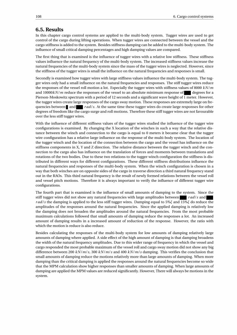
108 6. Cargo control systems
6.5. ResultsIn this chapter cargo control systems are applied to the multi-body system. Tugger wires are used to getcontrol of the cargo during lifting operations. When tugger wires are connected between the vessel and thecargo stiffness is added to the system. Besides stiffness damping can be added to the multi-body system. Theinfluence of small critical damping percentages and high damping values are compared.
The first thing that is examined is the influence of tugger wires with a relative low stiffness. These stiffnessvalues influence the natural frequency of the multi-body system. The increased stiffness values increase thenatural frequencies of the multi-body system since the mass of the tugger wires is neglected. However, sincethe stiffness of the tugger wires is small the influence on the natural frequencies and responses is small.
Secondly is examined how tugger wires with large stiffness values influence the multi-body system. The tug-ger wires only had a small influence on the natural frequencies and responses. The stiff tugger wires reducethe responses of the vessel roll motion a lot. Especially the tugger wires with stiffness values of 8000 kN /mand 10000kN /m reduce the responses of the vessel to an absolute minimum response of degrees for aPierson-Moskowitz spectrum with a period of 12 seconds and a significant wave height of 1 meter. However,the tugger wires create large responses of the cargo sway motion. These responses are extremely large on fre-quencies between and r ad/s. At the same time these tugger wires do create large responses for otherdegrees of freedom like the cargo surge and roll motions. Therefore these stiff tugger wires are not favourableover the less stiff tugger wires.
With the influence of different stiffness values of the tugger wires studied the influence of the tugger wireconfigurations is examined. By changing the X location of the winches in such a way that the relative dis-tance between the winch and connection to the cargo is equal to 0 meters it became clear that the tuggerwire configuration has a relative large influence on the response of the multi-body system. The location ofthe tugger winch and the location of the connection between the cargo and the vessel has influence on thestiffness components in X, Y and Z direction. The relative distance between the tugger winch and the con-nection to the cargo also has influence on the translation of forces and moments between translations androtations of the two bodies. Due to these two relations to the tugger winch configuration the stiffness is dis-tributed in different ways for different configurations. These different stiffness distributions influence thenatural frequencies and responses of the multi-body system. When the winch configuration is chosen in away that both winches are on opposite sides of the cargo in traverse direction a third natural frequency standout in the RAOs. This third natural frequency is the result of newly formed relations between the vessel rolland vessel pitch motions. Therefore it is always important to verify the influence of different tugger wireconfigurations.
The fourth part that is examined is the influence of small amounts of damping to the system. Since thestiff tugger wires did not show any natural frequencies with large amplitudes between r ad/s andr ad/s the damping is applied to the less stiff tugger wires. Damping equal to 5%ξ and 15%ξ do reduce theamplitudes of the responses around the natural frequencies. Since the applied damping is relatively lowthe damping does not broaden the amplitudes around the natural frequencies. From the most probablemaximum calculations followed that small amounts of damping reduce the responses a lot. An increasedamount of damping results in a increased amount of reduction of the response. However, the ratio withwhich the motion is reduce is also reduce.
Besides calculating the responses of the multi-body system for low amounts of damping relatively largeamounts of damping where applied. A side effect of the high amount of damping is that damping broadensthe width of the natural frequency amplitudes. Due to this wider range of frequency in which the vessel andcargo responded the most probable maximum of the vessel roll and cargo sway motion did not show any bigdifference between 200 kN /m/s, 300 kN /m/s and 400 kN /m/s damping. This verifies the conclusion thatsmall amounts of damping reduce the motions relatively more than large amounts of damping. When moredamping than the critical damping is applied the responses around the natural frequencies become so widethat the MPM calculation show higher responses than smaller amounts of damping. When large amounts ofdamping are applied the MPM values are reduced significantly. However, There will always be motions in thesystem.

7Discussion
Following the results from the sensitivity study and the tugger winch influence study there are several pointto discuss about the model.
Model validityFor every model applies the fact that the quality of the output of the model is directly proportional to thequality of the model and input. (garbage in, garbage out). This is also the case for this model. Since thefrequency domain is used to solve the responses there are some remarks on the validity of the model. Dueto the frequency domain all added parts had to be linear, all non-linear behaviour is linearizedor neglected.Higher order forces and motions are a non-linear problem. Therefore thee second order forces and motionscan not be calculated with this model. One example is the stiffness values of the pendulum, mooring linesand tugger winches. All these values are linearized and dependent on the responses of the different degreeof freedom. In reality these values are related to the sine/cosine function of the displacement or quadraticproportional to the elongation. Due to all these assumptions it might be useful to validate this model with avalidated computational model or model tests
Due to the linearization the stiffness and damping components in the multi-body system will have an influ-ence when there is a translation in positive or negative direction. Due to this linearization the influence ofmooring lines is not calculated correctly. When a mooring line falls slack stiffness is applied in this modelwhile this will not happen in real life. In the model tugger winches will apply stiffness throughout a wholecycle of the motions. In reality tugger winches may not be able to apply damping to the system at all times. Inreality the reduction due to damping can be lower than calculated by this model. Time domain simulationsor model tests can give more insight on the energy dissipation due to the systems described in this thesis. Afurther study regarding damping systems should be done before implementing such systems on-board of avessel.
Intended use of resultsThe tool creates more insight of the interaction between the different degrees of freedom. Although the re-sults only show the influence of certain measures on the multi-body system the different results show rela-tions between different measures and the reaction of the multi-body system. While the vessel hydrodynamicproperties are calculated by a 2D strip-theory program and all other relations are linearized the values willdiffer from reality. The results from this tool are meant to function as supporting information and should notfunction as a decision making tool. The master of the vessel is still responsible during lifting operations. Themaster should always consider possible risks during lifting operations. However, in the tool a lot of differentaspects are taken into account. In section 3.8 is shown that the mathematical linearization of the pendulumcreate accurate results for the natural frequencies of the multi-body system. section 3.9 showed that the re-sults of the Python tool and crane simulator have the same order of magnitude. This shows that the tool canbe used for for supporting information and until more detailed validation is done the results should not betaken as the absolute truth.
MPM valuesThe MPM values in this report showed mostly responsess above the 1 degree angle or 1 meter displacement.These values might feel large however these are values are the result of wave spectra with a wave height of1 meter. During lifting operations in ports the waves are broken. This results in lower wave heights duringlifting operations. The MPM values of the responses scale proportionate with the wave height. When thewave height during lifting operations are equal to 0.5 meters, twice as small in reality as in this report, theMPM values of the responses will also be twice as small as given in this report. Since linear theory is used theallowed sea state can also be calculated from the allowable MPM of a certain motion. equation 7.1 shows howthis can be done. In this equation HsSeaSt ate stands for the allowable wave height, MP MAll ow abl e represents
109

110 7. Discussion
the allowble MPM of the motion and MP MHs=1 represents the MPM of the corresponding motion for a seastate with the same period and a wave height of 1 meter.
HsSeaSt ate =MP MAll ow abl e
MP MHs=1
(7.1)
Wave spectraThe tool focuses on the multi-body system and the internal reaction between the different degrees of free-dom. External forces are not examined. During lifting operations the vessel will most likely operate in a portor an other, from weather protected, area. In these areas the wave spectrum will most likely differ from theJONSWAP and Pierson-Moskowitz spectra. Standing waves can also occur when waves are reflected by thequays. While the wave spectra differ from the wave spectra used in this study the results from the tool willdiffer from the motions in reality. This must be taken into account when the tool is used to calculate thevessel and cargo responses for accurate lifting operations. Alhough waves may differ at all different loadingoperations the RAOs still show how the vessel responds to different wave frequencies and wave directions.When the waves at loading cites can be described in a wavespectrum the MPM values can still be calculated.
Frequency domainMost of the assumptions made in this tool followed by the limitations of the frequency domain. All forcesand relations to forces had to be linearized. However, the frequency domain is still a good method to derivecharacteristic behaviours of a model. For a conceptual study and one of the fewer publicly available studiesthe frequency domain provides a lot of information. The non-linear components of the system are linearizedand therefore their influence is not fully neglected. With the linearization of the non-linear components theinfluence of these components are taken into account. A validated time-domain study can be done to validatethe influence of all the linearizations done in this model.
Use of the toolThis frequency domain model has shown useful results. The model did show the influence of different vari-ables during the lifting operation. Relations between lifting operation variables and the motions of the multi-body system could be formed from these results. The model can also be used to calculate the influence ofthese variables on lifting operations of future projects.
This tool did also show the influence of damping on both the vessel and cargo motions. According to the toolsmall amounts of damping will already have a large influence on the vessel and cargo motions. These resultscan be used for further studies when cargo control systems are developed for heavy lifting transport vessels.
Added value with respect to similar studiesWhen this thesis started not much, publicly available, research was done. Although advanced, third party,multi-body dynamics computation program might be able to solve the relation between vessel and cargodegrees of freedom these programs will most-likely not consist of a solver for hydrodynamic properties.Therefor, this study created new insight in the relation between loading conditions, lifting configurations andcargo-control systems. During this thesis other studies where released from embargo or released by heavylifting companies. Results from other studies regarding this topic are still hidden from public. Therefore itis hard to compare this research with research done by other companies. However, since it is one of the firstpublicly released studies regarding vessel lifting operations it will create a lot of insight for other studies.
The heavy lifting companies that already did a study regarding cargo control systems operate vessels that areonly designed for lifting operations and not for the transportation of cargo. Since these vessels are designedfor a different purpose these vessels will most likely respond in a different way on waves than the vesselsof BigLift Shipping. This study is the first study that looked at the influence of lifting operation motions forheavy lifting transport vessels.

8Conclusion
The purpose of this research can be split up in two parts. The first part of the research was gaining moreinsight on the relation between vessel motions and cargo motions during lifting operations. The second partof the research focused on reducing the motions of the two bodies during lifting operations.
The 12 degrees of freedom systemFor the first part of this study a model had to be written. By writing this model the interaction of the vesseland cargo motions had to be written in mathematical equations. Multi-body dynamics is used to solve theinteraction and calculate the responses of both bodies at the same time. By writing the natural behaviourit became clear that the cargo acted as a pendulum that was excited by the displacement of the crane tip.Before the influence of different lifting variables where studied baseline calculations were done in chapter4. In conventional calculations performed for lifting operations only 6 degrees of freedom are taken intoaccount. In the tool created for this thesis a 12 degrees of freedom multi-body system is used to calculate theresponses. In conventional calculations the dynamical aspects of the cargo are not taken into account. Themulti-body tool takes this influence into account. While both the conventional calculations and multi-bodysystem calculations have the same result for the natural frequency calculations for the 6 degrees of freedomof the vessel motions the multi-body system shows that the dynamical aspects of the cargo motions alsointroduce natural frequencies which also interact with the 6 degrees of freedom of the vessel motions. Allthese natural frequencies introduced by the dynamical aspects of the cargo motions can not be calculatedby the conventional tool. Thus conventional calculations fall short in calculating the natural frequencies andresponses of motions during lifting operations.
During this study it became clear that the vessel roll motion, cargo surge motion and cargo sway motion havethe largest amplitudes in the response amplitude operator calculations. All other degrees of freedom showedsmaller amplitudes and less extreme reactions on natural frequencies.
Besides the large amplitudes in the RAOs the vessel roll and cargo sway motion showed a large amount ofcoupling between the two degrees of freedom. The main excitation force of the cargo sway motion followsfrom the restoring force that is applied via the crane cable. In the case of the vessel roll and cargo sway motionthe stiffness value of this restoring force has the same order size as the hydrodynamical roll stiffness value.While both stiffness values have the same order size the influence of the coupling via the crane cable is largeon both degrees of freedom. This coupling enhances the responses of both degrees of freedom.
While the cargo surge motions RAO showed large peaks there was little coupling between the cargo surge mo-tion and other degrees of freedom. Mathematically the cargo sway motion showed identically large stiffnessvalues for the coupling via the crane cable to the vessel pitch motion as the cargo sway motion had with thevessel roll motion. However, the hydrodynamical vessel pitch stiffness values where an order size larger thanthe restoring stiffness values of the coupling between the cargo surge motion via the crane cable. While thestiffness values of the vessel pitch motion is an order size larger, the influence of the cargo surge motion onthe vessel pitch motion is small and both motions are only slightly enhanced by each other.
The multi-body tool created calculates more accurate responses than conventional calculations while muchmore aspects of a lifting operation are taken into account.
111

112 8. Conclusion
Wave directions and responsesIn chapter 4 the influence of different wave angles on the multi-body system are also calculated. While thevessel roll motion and cargo sway motion have a strong coupling waves with an angle perpendicular to thevessel causes the largest responses of the vessel and cargo motions. While this wave angle is used in therest of the thesis to calculate the influence of lifting variables and cargo control systems the study towardswave angles showed that all different wave angles can cause different degrees of freedom to show large RAOs.Therefor it is recommended to calculate the the responses of the multi-body system for different wave angleswhen this tool is used for lifting operations.
Influence of variables of the lifting operationThe influence of different variables of the lifting operation on the responses of the multi-body system arestudied in chapter 5. This study showed that the cargo mass, crane cable lenght, crane top Z position, cranetop Y position, and metacentric height of the vessel have relatively large influences on the natural frequenciesof the multi-body system. Some of these variables will stay constant during the lifting operation while otherswill vary during the operation.
The variables that will vary during a lifting operation are the crane cable length, crane top Z position andcrane top Y position. The vessels metacentric height can vary when water is pumped in to the ballast tankfrom outside the vessel. While these variables can change calculations with different variables should be donebefore a lifting operation is performed. In chapter 1 is explained that there are 5 different stages. For everystage a calculation with variables according to that stage should be done.
While some lifting variables will change in order to perform the lifting operation the tool can give valuableinsight in the lifting operation. The tool can be used to calculate the influence of using the forward or aftcrane or the influence or rotating the cargo clockwise or counterclockwise. When there is enough freedomduring a lifting operation the crane and rotation option can be chosen in such a way that the lowest motionsoccur.
The cargo mass will not vary during a lifting operation. However this variable will be different for every dif-ferent lifting operation. While all different lifting operations varies from each other the lifting calculationsshould be done for all different lifting operations. Results for previously calculated lifting operations are notsufficient for new lifting operations.
Mooring linesThe influence of mooring lines are also studied in chapter 5. While normal mooring lines do not influence themulti-body system very much very stiff mooring configurations influence the responses a lot. When mooringlines with short lengths are connected between the vessel and shore the stiffness of these lines are large. Theselarge stiffness values increase the natural frequencies of the multi-body system. Besides these increased nat-ural frequencies the amplitudes of the motions are also increased. The mooring lines couple the vessel swaymotions to vessel roll motions. While vessel sway motions are inhibited the responses of the vessel roll mo-tions are increased, which also increases the responses of the cargo sway motion. Therefor it can be con-cluded that a stiff mooring line configuration deliver no reduction of the vessel and cargo motions duringlifting operations in waves.
Cargo control systemsThe model used to calculate the influence between the different degrees of freedom in the vessel-cargo sys-tem is expanded with systems to control the cargo motions. Currently the most widespread practice is the useof tugger winches. These winches add additional stiffness to the vessel-cargo system. The implementation ofthe cargo control system showed that only adding stiffness to the multi-body system will not result in lowermotions during lifting operations.
Besides the influence of conventional tugger winches the influence of damping is examined. Damping addedvia the tugger winches influence the responses around the natural frequencies. Especially small amountsof damping have a relative large influence on the responses of the vessel and cargo. This shows that smallamounts of damping can be usefull during lifting operations.

113
This study showed that adding damping to the system will reduce the cargo motions. Besides the reductionof the cargo motions the vessel motions are reduced. Especially the vessel roll motion. While the vessel rollmotion has a strong coupling to the cargo sway motion a reduction of the cargo sway motion results in areduction of the vessel roll motion. This study showed that adding damping to the system can be useful toincrease the safety and workabiltiy during lifting operations.
Overall conclusionThe overall conclusion form this research is that it is useful to look at the different variables of the multi-bodysystem. The conventional 6 degrees of freedom stability calculations fall to short when the responses of thevessel are calculated during lifting operations. The dynamical aspects of the cargo hanging from the cranecan have a large influence on the vessel motions, especially when the cargo has a large mass.
The study did also show that small amounts of damping can heavily influence the multi-body system of boththe vessel and cargo motions. Besides the damping of the cargo motions the vessel motions are reduced whenthe cargo is damped. This study showed that it is useful to apply small amounts of damping to the multi-bodysystem to increase the safety and workability during lifting operations.
Even though the model created for the calculations and used for creating the results of this research is afrequency domain model the different results showed large influences of the implementation of a multi-bodysystem, variables of the multi-body system and damping. Because the model already showed large influencesit shows that the frequency domain method can be a useful method to study the behaviour of the multi-bodysystem.
By creating this tool and using this tool to examine the influence of the interaction of the vessel and cargo,the different variables during lifting operations and cargo-control mechanisms, it is proven that the tool is avaluable extension to BigLift’s engineering methods. This tool can be used to predict vessel and cargo motionsduring lifting operations in waves. The creation of this tool and the results from the tool fulfilled the thesisobjective.
"Determine the influence of vessel motions on cargo motions on each other during lifting operations in wavesand develop a method to decrease the motions during lifting operations in waves"
While the thesis objective is fulfilled the presented tool provides insight and creates more knowledge regard-ing lifting operations in waves. The tool forms a bridge between used practices, mathematical knowledge andphysical relations. The tool also showed how different methods can be used to decrease the responses of themultiple degrees of freedom during lifting operations.


Bibliography
[1] R.I. Cambero and Sausedo-Solorio J.M. Dynamics of the shift in resonance frequency in a triple pendu-lum. Meccanica, 2011.
[2] G.F. Claus and M Vannahme. Experimental study of the nonlinear dynamics of floating cranes. The ninthinternational offshore and polar engineering conference, 1999.
[3] Dr. I. Dmitrieva. DELFRAC. Tu Delft, 1994.
[4] Greenwood D.T. Advanced Dynamics. Cambridge University Press, 2003.
[5] O.M. Faltinesen. Sea loads on ships and offshore structures. Cambridge University Press, Cambridge, UK,1990.
[6] J.F. Flory, S.P. Banfield, and Dr. A. Ractliffe. Computer mooring load analysis to improve port operationsand safety, 2013. URL https://www.tensiontech.com/papers/optimoor.
[7] Python Software Foundation. PythonTM, 2019. URL https://www.python.org/doc/.
[8] G. González. A pendulum with a moving support point, 2006. URL http://www.phys.lsu.edu/faculty/gonzalez/Teaching/Phys7221/PendulumWithMovingSupport.pdf.
[9] J. Healy. Eigen what?, 2017. URL https://www.physicssayswhat.com/2017/03/24/eigen-what/.
[10] J.W.A.M. IJzermans. Heavy lifting during wave exposure. Master’s thesis, TU Delft, 2005.
[11] J.M.J. Journee. User manual of Seaway. Tu Delft, 2001.
[12] J.M.J. Journée and W.W. Massie. OFFSHORE HYDROMECHANICS. Wiley, 2007.
[13] Y. Kawahara, K. MAEKAWA, and Y. IKEDA. A simple prediction formula of roll damping of conventionalcargo ships on the basis of ikeda’s method and its limitation. Proceedings of the 10th International Con-ference on Stability of Ships and Ocean Vehicles, 2010.
[14] L.A. Ladino and H.S. Rondón. Determining the damping coefficient of a simple pendulum oscillating inair. Physics Educatoin Educ. 52, 2007.
[15] H. Lageveen. Modelling and steering of tuggerwinches. Master’s thesis, TU Delft, 2014.
[16] This Condensed Life. Phase difference after resonance, 2016. URL https://thiscondensedlife.wordpress.com/2016/05/02/phase-difference-after-resonance/.
[17] LLoyd’s Register Group LTD. Lloyd’s register rules and regulations - rules and regulations for the classifi-cation of ships, 2017.
[18] D.J.C. MacKay. Normal modes and the douple pendulum, 2001. URL http://www.inference.org.uk/teaching/dynamics/course.html.
[19] G. Meskers and R. van Dijk. A damping tugger system for offshore heavy lifts. OMAE, 2012.
[20] A. Montanari. Mechanics of sea waves, 2017. URL https://distart119.ing.unibo.it/albertonew/?q=node/104.
[21] A. Montanari. Ocean-wave spectra, 2017. URL https://distart119.ing.unibo.it/albertonew/?q=node/104.
[22] BEXCOZ N.V. DeepRope Polyester & Dyneema mooring ropes manual 2004. Le Lis, 2015.
115

116 Bibliography
[23] M.K. Ochi. On prediction of extreme values. Journal of Ship Research, 1973.
[24] M.K. Ochi. Principles of extreme value statistics and their application. The society of naval architects andmarine engineers, 1981.
[25] Katsuhiko Ogata. System Dynamics (4th ed.). University of Minnesota, 2005.
[26] M.J. Ormond. Depth compensated subsea passive heave compensator, 2014. URL http://www.ipaustralia.com.au/applicant/intermoor-inc/patents/AU2009233731/.
[27] Jasna. Prpic-Oršic, V. Slapnicar, and A. Turk. Berth operability estimation related to ship mo-tion, 2014. URL https://www.researchgate.net/publication/291342321_Berth_operability_estimation_related_to_ship_motion.
[28] S.S. RAO. Mechanical Vibrations. Prentice-Hall Inc., 2004.
[29] R Rubenzahl and S.G. Rajeev. Small oscillations of the n-pendulum and the "hanging rope" limit n →∞.http://www.pas.rochester.edu/~rrubenza/projects/RR_PHY235W_TermPaper.pdf, 2017.
[30] BigLift Shipping. Biglift compony profile, 2019. URL https://www.bigliftshipping.com/en/company/profile.
[31] D. Skandali. Identification of response amplitude operators for ships based on full scale measurements.Master’s thesis, TU Delft, 2015.
[32] M. St. Denis and W.J. Pierson. On the motion of ships in confused seas. Vol. 61, pages 1–53, 1953.
[33] Stackexchange physics. Critical damping ratios and oscillations plot-ted, 2014. URL https://physics.stackexchange.com/questions/106091/faster-than-critical-damping-for-harmonic-oscillator.
[34] P.P. Urone, P. Hinrichs, K. Dirks, and M. Sharma. Adiabatic processes of an ideal gas,2019. URL https://phys.libretexts.org/Bookshelves/University_Physics/Book%3A_University_Physics_(OpenStax)/Map%3A_University_Physics_II_-_Thermodynamics%2C_Electricity%2C_and_Magnetism_(OpenStax)/3%3A_The_First_Law_of_Thermodynamics/3.6%3A_Adiabatic_Processes_for_an_Ideal_Gas.
[35] E.F.G. van Daalen. MARIN Shipmo User Manual. MARIN, 2015.
[36] Y. Wang, A. van Deyzen, and B. Beimers. Less=moor: A time-efficient computational tool to assess thebehavior of moored ships in waves. Physics Educatoin Educ. 52, 2007.
[37] F.E. Wester. Heave compensated floatover operation. Master’s thesis, TU Delft, 2015.
[38] F.M. White. Fluid Mechanics. McGraw-Hill, New York, NY, 7 edition, 2011.
[39] Wikipedia. Metacentric height, 2019. URL https://en.wikipedia.org/wiki/Metacentric_height.
[40] D. Wood. The superposition principle & resultant waves, 2019. URL https://study.com/academy/lesson/the-superposition-principle-resultant-waves.html.
[41] J.K. Woodacre, R.J. Bauer, and R.A. Irani. A review of vertical motion heave compensation systems. OceanEngineering 104, pages 140–154, 2015.
[42] Q. Yuan. Actively damped heave compensation (adhc) system. Proceedings of the 2010 American ControlConference, pages 1544–1549, 2010.

AFree body diagrams
A.1. Free body diagrams crane cable connection
(a) Free body diagram of the interaction between thevessel and cargo via the crane cable for the surge motion
of the vessel (X1)
(b) Free body diagram of the interaction between thevessel and cargo via the crane cable for the sway motion
of the vessel (X2)
Figure A.1: The two free body diagrams of the interaction between the vessel and cargo via the crane cable or the surge motion of thevessel and the sway motion of the vessel
117

118 A. Free body diagrams
(a) Free body diagram for of the interaction betweenthe vessel and cargo via the crane cable the heave
motion of the vessel (X3)
(b) Free body diagram for of the interaction betweenthe vessel and cargo via the crane cable the roll
motion of the vessel (X4)
Figure A.2: The two free body diagrams of the interaction between the vessel and cargo via the crane cable for the heave motion of thevessel and the roll motion of the vessel
(a) Free body diagram for of the interaction betweenthe vessel and cargo via the crane cable the pitch
motion of the vessel (X5)
(b) Free body diagram for of the interaction betweenthe vessel and cargo via the crane cable the yaw
motion of the vessel (X6)
Figure A.3: The two free body diagrams of the interaction between the vessel and cargo via the crane cable for the pitch motion of thevessel and the yaw motion of the vessel

A.1. Free body diagrams crane cable connection 119
(a) Free body diagram for of the interaction betweenthe vessel and cargo via the crane cable the surge
motion of the cargo (X7)
(b) Free body diagram for of the interaction betweenthe vessel and cargo via the crane cable the sway
motion of the cargo (X8)
Figure A.4: The two free body diagrams of the interaction between the vessel and cargo via the crane cable for the surge motion of thecargo and the sway motion of the cargo
(a) Free body diagram for the heave motion of thecargo (X9)
Figure A.5: The free body diagram of the interaction between the vessel and cargo via the crane cable for the heave motion of the vesseland the roll motion of the vessel

120 A. Free body diagrams
A.2. Free body diagrams mooring line connection
(a) Free body diagram of the interaction between thevessel and the shore via mooring lines for the surge
motion of the vessel (X1)
captionFree body diagram of the interactionbetween the vessel and the shore via mooring
lines for the sway motion of the vessel (X2)
Figure A.6: The two free body diagrams of the interaction between the vessel and the shore via mooring lines for the surge motion of thevessel and the sway motion of the vessel
(a) Free body diagram of the interaction between thevessel and the shore via mooring lines for the heave
motion of the vessel (X3)
captionFree body diagram of the interactionbetween the vessel and the shore via mooring
lines for the roll motion of the vessel (X4)
Figure A.7: The two free body diagrams of the interaction between the vessel and the shore via mooring lines for the heave motion ofthe vessel and the roll motion of the vessel

A.2. Free body diagrams mooring line connection 121
(a) Free body diagram of the interaction between thevessel and the shore via mooring lines for the pitch
motion of the vessel (X5)
captionFree body diagram of the interactionbetween the vessel and the shore via mooring
lines for the yaw motion of the vessel (X6)
Figure A.8: The two free body diagrams of the interaction between the vessel and the shore via mooring lines for the pitch motion of thevessel and the yaw motion of the vessel

122 A. Free body diagrams
A.3. Free body diagrams cargo control system connection
(a) Free body diagram of the interaction between thevessel and the cargo via cargo control systems for the
surge motion of the vessel (X1)
(b) Free body diagram of the interaction between thevessel and the cargo via cargo control systems for the
sway motion of the vessel (X2)
Figure A.9: The two free body diagrams of the interaction between the vessel and the cargo via cargo control systems for the surgemotion of the vessel and the sway motion of the vessel

A.3. Free body diagrams cargo control system connection 123
(a) Free body diagram of the interaction between thevessel and the cargo via cargo control systems for the
heave motion of the vessel (X3)
(b) Free body diagram of the interaction between thevessel and the cargo via cargo control systems for the
roll motion of the vessel (X4)
Figure A.10: The two free body diagrams of the interaction between the vessel and the cargo via cargo control systems for the heavemotion of the vessel and the roll motion of the vessel
(a) Free body diagram of the interaction between thevessel and the cargo via cargo control systems for the
pitch motion of the vessel (X5)
(b) Free body diagram of the interaction between thevessel and the cargo via cargo control systems for the
yaw motion of the vessel (X6)
Figure A.11: The two free body diagrams of the interaction between the vessel and the cargo via cargo control systems for the pitchmotion of the vessel and the yaw motion of the vessel

124 A. Free body diagrams
(a) Free body diagram of the interaction between thevessel and the cargo via cargo control systems for the
surge motion of the cargo (X7)
(b) Free body diagram of the interaction between thevessel and the cargo via cargo control systems for the
sway motion of the cargo (X8)
Figure A.12: The two free body diagrams of the interaction between the vessel and the cargo via cargo control systems for the surgemotion of the cargo and the sway motion of the cargo
(a) Free body diagram of the interaction between thevessel and the cargo via cargo control systems for the
heave motion of the cargo (X9)
(b) Free body diagram of the interaction between thevessel and the cargo via cargo control systems for the
roll motion of the cargo (X10)
Figure A.13: The two free body diagrams of the interaction between the vessel and the cargo via cargo control systems for the heavemotion of the cargo and the roll motion of the cargo

A.3. Free body diagrams cargo control system connection 125
(a) Free body diagram of the interaction between thevessel and the cargo via cargo control systems for the
pitch motion of the cargo (X11)
(b) Free body diagram of the interaction between thevessel and the cargo via cargo control systems for the
yaw motion of the cargo (X12)
Figure A.14: The two free body diagrams of the interaction between the vessel and the cargo via cargo control systems for the pitchmotion of the vessel and the yaw motion of the cargo


BMatrices
M11 0 0 0 0 0 0 0 0 0 0 00 M22 0 M24 0 M26 0 0 0 0 0 00 0 M33 0 M35 0 0 0 0 0 0 00 M42 0 M44 0 M46 0 0 0 0 0 00 0 M53 0 M55 0 0 0 0 0 0 00 M62 0 M64 0 M66 0 0 0 0 0 00 0 0 0 0 0 M77 0 0 0 0 00 0 0 0 0 0 0 M88 0 0 0 00 0 0 0 0 0 0 0 M99 0 0 00 0 0 0 0 0 0 0 0 M1010 0 00 0 0 0 0 0 0 0 0 0 M1111 00 0 0 0 0 0 0 0 0 0 0 M1212
M11 = Mhyd11 + Ahyd11
M22 = Mhyd22 + Ahyd22
M24 = Ahyd24
M26 = Ahyd26
M33 = Mhyd33 + Ahyd33
M35 = Ahyd35
M42 = Ahyd42
M44 = Mhyd44 + Ahyd44
M46 = Ahyd46
M53 = Ahyd53
M55 = Mhyd55 + Ahyd55
M62 = Ahyd62
M64 = Ahyd64
M66 = Mhyd66 + Ahyd66
M77 = Mpen
M88 = Mpen
M99 = Mpen
M1010 = IpenX
M1111 = IpenY
M1212 = IpenZ
127

128 B. Matrices
B11 0 0 0 B15 B16 B17 0 0 0 B111 B112
0 B22 0 B24 0 B26 0 B28 0 B210 0 B212
0 0 B33 B34 B35 0 0 0 B39 B310 B311 00 B42 B43 B44 B45 B46 0 B48 B49 B410 B411 B412
B51 0 B53 B54 B55 B56 B57 0 B59 B510 B511 B512
B61 B62 0 B64 B65 B66 B67 B68 0 B610 B611 B612
B71 0 0 0 B75 B76 B77 0 0 0 B711 B712
0 B82 0 B84 0 B86 0 B88 0 B810 0 B812
0 0 B93 B94 B95 0 0 0 B99 B910 B911 00 B102 B103 B104 B105 B106 0 B108 B109 B1010 B1011 B1012
B111 0 B113 B114 B115 B116 B117 0 B119 B1110 B1111 B1112
B121 B122 0 B124 B125 B126 B127 B128 0 B1210 B1211 B1212
B11 = Bhyd11 +Btug g er11
B15 = Btug g er15
B16 = Btug g er16
B17 = Btug g er17
B111 = Btug g er111
B112 = Btug g er112
B22 = Bhyd22 +Btug g er22
B24 = Bhyd24 +Btug g er24
B26 = Bhyd26 +Btug g er26
B28 = Btug g er28
B210 = Btug g er210
B212 = Btug g er212
B33 = Bhyd33 +Btug g er33
B34 = Btug g er34
B35 = Bhyd35 +Btug g er35
B39 = Btug g er39
B310 = Btug g er310
B311 = Btug g er311
B42 = Bhyd42 +Btug g er42
B43 = Btug g er43
B44 = Bhyd44 +Btug g er44
B45 = Btug g er45
B46 = Bhyd46 +Btug g er46
B48 = Btug g er48
B49 = Btug g er49
B410 = Btug g er410
B411 = Btug g er411
B412 = Btug g er412
B51 = Btug g er51
B53 = Bhyd53 +Btug g er53
B54 = Btug g er54
B55 = Bhyd55 +Btug g er55
B56 = Btug g er56
B57 = Btug g er57
B59 = Btug g er59
B510 = Btug g er510
B511 = Btug g er511
B512 = Btug g er512
B61 = Btug g er61
B62 = Bhyd62 +Btug g er62
B64 = Bhyd64 +Btug g er64
B65 = Btug g er65
B66 = Bhyd66 +Btug g er66
B67 = Btug g er67
B68 = Btug g er68
B610 = Btug g er610
B611 = Btug g er611
B612 = Btug g er612
B71 = Btug g er71
B75 = Btug g er75
B76 = Btug g er76
B77 = Bai r77 +Btug g er77
B711 = Btug g er711
B712 = Btug g er712
B82 = Btug g er82
B84 = Btug g er84
B86 = Btug g er86
B88 = Bai r88 +Btug g er88
B810 = Btug g er810
B812 = Btug g er812
B93 = Btug g er93
B94 = Btug g er94
B95 = Btug g er95
B99 = Bai r99 +Btug g er99
B910 = Btug g er910
B911 = Btug g er911
B102 = Btug g er102
B103 = Btug g er103
B104 = Bai r1010 +Btug g er104
B105 = Btug g er105
B106 = Btug g er106
B108 = Btug g er108
B109 = Btug g er109
B1010 = Btug g er1010
B1011 = Btug g er1011
B1012 = Btug g er1012
B111 = Btug g er111
B113 = Btug g er113
B114 = Btug g er114
B115 = Btug g er115
B116 = Btug g er116
B117 = Btug g er117
B119 = Btug g er119
B1110 = Btug g er1110
B1111 = Bai r1111 +Btug g er1111
B1112 = Btug g er1112
B121 = Btug g er121
B122 = Btug g er122
B124 = Btug g er124
B125 = Btug g er125
B126 = Btug g er126
B127 = Btug g er127
B128 = Btug g er128
B1210 = Btug g er1210
B1211 = Btug g er1211
B1212 = Bai r1212 +Btug g er1212
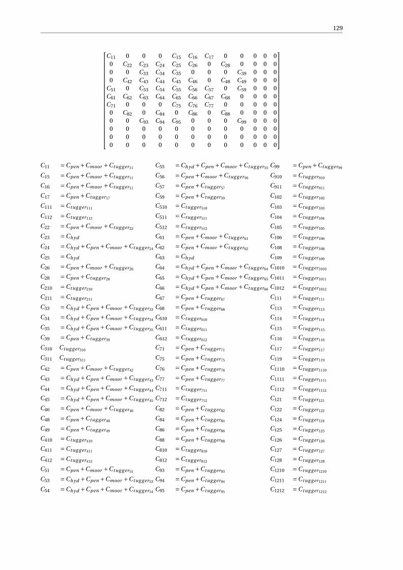
129
C11 0 0 0 C15 C16 C17 0 0 0 0 00 C22 C23 C24 C25 C26 0 C28 0 0 0 00 0 C33 C34 C35 0 0 0 C39 0 0 00 C42 C43 C44 C45 C46 0 C48 C49 0 0 0
C51 0 C53 C54 C55 C56 C57 0 C59 0 0 0C61 C62 C63 C64 C65 C66 C67 C68 0 0 0 0C71 0 0 0 C75 C76 C77 0 0 0 0 0
0 C82 0 C84 0 C86 0 C88 0 0 0 00 0 C93 C94 C95 0 0 0 C99 0 0 00 0 0 0 0 0 0 0 0 0 0 00 0 0 0 0 0 0 0 0 0 0 00 0 0 0 0 0 0 0 0 0 0 0
C11 =Cpen +Cmoor +Ctug g er11
C15 =Cpen +Cmoor +Ctug g er11
C16 =Cpen +Cmoor +Ctug g er11
C17 =Cpen +Ctug g er17
C111 =Ctug g er111
C112 =Ctug g er112
C22 =Cpen +Cmoor +Ctug g er22
C23 =Chyd
C24 =Chyd +Cpen +Cmoor +Ctug g er24
C25 =Chyd
C26 =Cpen +Cmoor +Ctug g er26
C28 =Cpen +Ctug g er28
C210 =Ctug g er210
C211 =Ctug g er211
C33 =Chyd +Cpen +Cmoor +Ctug g er33
C34 =Chyd +Cpen +Cmoor +Ctug g er34
C35 =Chyd +Cpen +Cmoor +Ctug g er35
C39 =Cpen +Ctug g er39
C310 Ctug g er310
C311 Ctug g er311
C42 =Cpen +Cmoor +Ctug g er42
C43 =Chyd +Cpen +Cmoor +Ctug g er43
C44 =Chyd +Cpen +Cmoor +Ctug g er44
C45 =Chyd +Cpen +Cmoor +Ctug g er45
C46 =Cpen +Cmoor +Ctug g er46
C48 =Cpen +Ctug g er48
C49 =Cpen +Ctug g er49
C410 =Ctug g er410
C411 =Ctug g er411
C412 =Ctug g er412
C51 =Cpen +Cmoor +Ctug g er51
C53 =Chyd +Cpen +Cmoor +Ctug g er53
C54 =Chyd +Cpen +Cmoor +Ctug g er54
C55 =Chyd +Cpen +Cmoor +Ctug g er55
C56 =Cpen +Cmoor +Ctug g er56
C57 =Cpen +Ctug g er57
C59 =Cpen +Ctug g er59
C510 =Ctug g er510
C511 =Ctug g er511
C512 =Ctug g er512
C61 =Cpen +Cmoor +Ctug g er61
C62 =Cpen +Cmoor +Ctug g er62
C63 =Chyd
C64 =Chyd +Cpen +Cmoor +Ctug g er64
C65 =Chyd +Cpen +Cmoor +Ctug g er65
C66 =Chyd +Cpen +Cmoor +Ctug g er66
C67 =Cpen +Ctug g er67
C68 =Cpen +Ctug g er68
C610 =Ctug g er610
C611 =Ctug g er611
C612 =Ctug g er612
C71 =Cpen +Ctug g er71
C75 =Cpen +Ctug g er75
C76 =Cpen +Ctug g er76
C77 =Cpen +Ctug g er77
C711 =Ctug g er711
C712 =Ctug g er712
C82 =Cpen +Ctug g er82
C84 =Cpen +Ctug g er84
C86 =Cpen +Ctug g er86
C88 =Cpen +Ctug g er88
C810 =Ctug g er810
C812 =Ctug g er812
C93 =Cpen +Ctug g er93
C94 =Cpen +Ctug g er94
C95 =Cpen +Ctug g er95
C99 =Cpen +Ctug g er99
C910 =Ctug g er910
C911 =Ctug g er911
C102 =Ctug g er102
C103 =Ctug g er103
C104 =Ctug g er104
C105 =Ctug g er105
C106 =Ctug g er106
C108 =Ctug g er108
C109 =Ctug g er109
C1010 =Ctug g er1010
C1011 =Ctug g er1011
C1012 =Ctug g er1012
C111 =Ctug g er111
C113 =Ctug g er113
C114 =Ctug g er114
C115 =Ctug g er115
C116 =Ctug g er116
C117 =Ctug g er117
C119 =Ctug g er119
C1110 =Ctug g er1110
C1111 =Ctug g er1111
C1112 =Ctug g er1112
C121 =Ctug g er121
C122 =Ctug g er122
C124 =Ctug g er124
C125 =Ctug g er125
C126 =Ctug g er126
C127 =Ctug g er127
C128 =Ctug g er128
C1210 =Ctug g er1210
C1211 =Ctug g er1211
C1212 =Ctug g er1212


CEquations of Motion
Table C.1: Definition of abbreviations used in the equations of motion
Abbreviation Meaning / Definition
Fexcn Excitation forces of the n-th degree of freedom
xn Response of the n-th degree of freedom.
Mhydnm Hydrodynamic mass values. Influence of m-th degree of freedom on the n-th
degree of freedom
Ahydnm Hydrodynamic added mass values. Influence of m-th degree of freedom on
the n-th degree of freedom
Bhydnm Hydrodynamic damping values. Influence of m-th degree of freedom on the
n-th degree of freedom
Bai rnm Air damping of the pendulum motions.
Btugx y z Damping values of the damping applied via the tugger winch system in x,y,
and z direction respectively
Chydnm Hydrodynamic restoring stiffness values. Influence of m-th degree of freedom
on the n-th degree of freedom
Kpen Restoring stiffness value of the cargo pendulum motion
Kwi r e Wire stiffness of the crane cable
Kmoorx y z Restoring stiffness value of a mooring line in x, y, and z direction respectively
Ktugx y z Restoring stiffness value of the tugger wires in x, y, and z direction respectively
Xcr ,Ycr , Zcr X, Y, and Z position of the crane tip
Xwi nch ,Ywi nch , Zwi nch X, Y, and Z position of the fairlead of the mooring line respectively to the cen-
tre of gravity of the vessel.
X tug ,Ytug , Ztug X, Y, and Z position of the tugger winch respectively to the centre of gravity of
the vessel
Xpad ,Ypad , Zpad X, Y, and Z position of the connection of the tugger wire to the cargo
131

132 C. Equations of Motion
Surge vessel
Fexc1 =−ω2 · (Mhyd11 + Ahyd11
) · x1
− iω · ((Bhyd11 +∑(
Btugx
)) · x1 +(∑(
Btugx ·Ztug)) · x5 −
(∑(Btugx ·Ytug
)) · x6
− (∑(Btugx
)) · x7 −(∑(
Btugx ·Zpad)) · x11 +
(∑(Btugx ·Ypad
)) · x12)
+ (Kpen +∑
Kmoorx +∑
Ktugx
) · x1 +(Kpen ·ZCr +
∑(Kmoorx ·ZW i nch
)+∑(Ktugx ·Ztug
)) · x5
− (Kpen ·Cr aneY +∑(
Kmoorx ·YW i nch)+∑(
Ktugx ·Ytug)) · x6 −
(Kpen +∑
Kpenx
) · x7
− (∑((Ktugx ·Zpad
))x11 +
(∑((Ktugx ·Ypad
)) · x12
(C.1)
Sway vessel
Fexc2 =−ω2 · ((Mhyd22 + Ahyd22
) · x2 + Ahyd24 · x4 + Ahyd26 · x6)
− iω ·((
Bhyd22 +∑
Btug y
)· x2 +
(Bhyd24 −
∑(Btug y ·Ztug
))· x4 +
(Bhyd26 +
∑(Btug y ·X tug
))· x6
−∑Btug y · x8 +
∑(Btug y ·Zpad
)· x10 −
∑(Btug y ·Xpad
)· x12
)+ (
Kpen +∑KmoorY +∑
KtugY
) · x2 −(Kpen ·ZCr +
∑(KmoorY ·Zwi nch
)+∑(KtugY ·Ztug
)) · x4+(Kpen ·XCr +
∑(KmoorY ·XW i nch
)+∑(Ktug y ·X tug
))· x6 −
(Kpen +Ktug y
)· x8
+(∑(
Ktug y ·Zpad
))· x10 −
(∑(Ktug y ·Xpad
))· x12
(C.2)
Heave vessel
Fexc3 =−ω2 · (((Mhyd33 + Ahyd33
) · x3 + Ahyd35 · x5)
− iω((
Bhyd33 +∑(
Btugz
)) · x3 +(∑(
Btugz ·Ytug)) · x4 +
(Bhyd35 −
∑(Btugz ·X tug
)) · x5
− (∑(Ktugz
)) · x9 −(∑(
Ktugz ·Ypad)) · x10 +
(∑(Ktugz ·Xpad
)) · x11)
+ (Kwi r e +
∑KmoorZ +∑
Ktugz
) · x3 +(Kwi r e ·YCr +
∑(KmoorZ ·YW i nch
)+∑(Ktugz ·Ytug
)) · x4
− (Kwi r e ·Xcr +
∑(KmoorZ ·Xwi nch
)+∑(Ktugz ·X tug
)) · x5 −(Kwi r e +Ktugz
) · x9
− (∑(Ktugz ·Ypad
)) · x10 +(∑(
Ktugz ·Xpad)) · x11
(C.3)

133
Roll vessel
Fexc4 =−ω2 · (A42 · x2 + (M44 + A44) · x4 + A46 · x6)−− iω
((Bhyd42 −
∑(Btug y ·Ytug
))· x2 +
(∑(Btugz ·Ytug
)) · x3
+(Bhyd44 +
(∑(Btug y ·Z 2
tug
))(∑(Btugz ·Y 2
tug
)))· x4
−(∑(Btugz ·X tug ·Ytug
)) · x5 +(B46 −
(∑(BTug y ·X tug ·Ztug
)))· x6
+(∑(
Btug y ·Zwi nch
))x8 −
(∑(Btugz ·Ywi nch
))x9
+(∑(
Btug y ·Zpad ·Ztug
)+∑(
Btugz ·Ypad ·Ytug)) · x10
+ (∑(Btugz ·Xpad ·Ytug
)) · x11 −(∑(
Btug y ·Xpad ·Ztug
))· x12
)− (
Kpen ·ZcrZ +∑(KmoorY ·Zwi nch
)+ (∑(Kt ug y Ztug
))) · x2+(Chyd43 +Kwi r e ·Ycr +
(∑(KmoorZ ·W i nchY
))+ (∑(Ktugz ·Ytug
))) · x3
+ (Chyd44 +Kpen ·Z 2
cr +Kwi r e ·Y 2cr +
(∑(KmoorZ ·Y 2
wi nch
))+ (∑(KmoorY ·Z 2
wi nch
))+
(∑(Ktug y ·Z 2
tug
))+
(∑(Ktugz Y 2
tug
)))· x4
− (Chyd45 +Kwi r e ·Xcr ·Ycr +
∑(KmoorZ ·Xwi nch ·Ywi nch
)+ (∑(Ktugz ·X tug ·Ytug
))) · x5
−(Kpen ·Xcr ·Zcr +
∑(Kl i neZ ·Xwi nch ·Zwi nch
)+ (∑(Ktug y ·X tug ·Ztug
)))· x6
+((
Kpen ·Zcr)+ (∑(
Ktug y ·Zwi nch
)))· x8 −
((Kwi r e ·Xcr )+ (∑(
Ktugz ·Ywi nch))) · x9
−((∑(
Ktug y ·Zpad ·Ztug
))+ (∑(
Ktugz ·Ypad ·Ytug))) · x10
+ (∑(Ktugz ·Xpad ·Ytug
)) · x11 −(∑(
Ktug y ·Xpad ·Ztug
))· x12
(C.4)
Pitch vessel
Fexc5 =−ω2 · (A53 · x3 + (M55 + A55) · x5)
− iω(∑(
Btugx ·Ztug) · x1 +
(B53 −
∑(Btugz ·X tug
)) · x3 −∑(
Btugz ·Ytug ·X tug) · x4
+(B55 +
∑(Btugx ·Z 2
tug
)+∑(
Btugz ·X 2tug
))· x5 −
∑(Btugx ·Ytug ·Ztug
) · x6
−∑(Btugx ·Zwi nch
) · x7 +∑(
Btugz ·Zwi nch) · x9 +
∑(Btugz ·Ypad ·X tug
) · x10
−(∑(BTugx ·Zpad ·Ztug
)+∑(Btugz ·Xpad ·X tug
)) · x11 +∑(
Btugx ·Ypad ·Zpad) · x12
)(Kpen ·Cr aneZ +∑(
Kmoorx ·Zwi nch)+∑(
Ktugx ·Ztug)) · x1+(
Chyd53 −Kwi r e ·Xcr −∑(
KmoorZ ·Xwi nch)−∑(
Ktugz ·X tug)) · x3
+ (Chyd54 −Kwi r e ·Ycr ·Xcr −
∑(KmoorY ·Ywi nch ·Xwi nch
)−∑(Ktugz ·Ytug ·X tug
)) · x4
+ (Chyd55 +Kpen ·Z 2
cr +Kwi r e ·X 2cr
+ ∑(KmoorX ·Z 2
wi nch
)+∑(KmoorZ ·X 2
wi nch
)+∑(Ktugx ·Z 2
tug
)+∑(
Ktugz ·X 2tug
))· x5
− (Kpen ·Ycr ·Zcr +
∑(KmoorX ·Ywi nch ·Zwi nch
)+∑(Ktugx ·Ytug ·Ztug
)) · x6
− (Kpen ·Zcr +
∑(Ktugx ·Zwi nch
)) · x7 +(Kpen ·Xcr +
∑(Ktugz ·Xwi nch
)) · x9
+∑(Ktugz ·Ypad ·Xpad
) · x10 −(∑(
Ktugx ·Zpad ·Ztug)+∑(
KtugZ ·Xpad ·X tug)) · x11
+∑(Ktugx ·Ypad ·Ztug
) · x12
(C.5)

134 C. Equations of Motion
Yaw vessel
Fexc6 =−ω2 · (A62 · x2 + A54 · x4 + (M66 + A66) · x6)
− iω ·(−∑(
Btugx ·Ytug) · x1 +
(B62 +
∑(Btug y ·X tug
))· x2 +
(B64 −
∑(Btug y ·Ztug ·X tug
))· x4
+∑(Btugx ·Ztug ·Ytug
) · x5 +(B66 +
∑(Btug y ·X 2
tug
)+∑(
BtugX ·Y 2tug
))· x6
+∑(Btugx ·Ywi nch
) · x7 −∑(
Btug y ·Xwi nch
)· x8 +
∑(Btug y ·Zpad ·X tug
)· x10
−∑(Btugx ·Zpad ·Ytug
) · x11 −(∑(
Btug y ·Xpad ·X tug
)+∑(
Btugx ·Ypad ·Ytug)) · x12
)+ (
Kpen ·Ycr −∑(
KmoorX ·Ywi nch)−∑(
Ktugx ·Ztug)) · x1
+(Kpen ·Xcr +
∑(KmoorY ·Xwi nch
)+∑(Ktug y ·X tug
))· x2 +Chyd63 · x3
+(Chyd64 −Kpen ·Zcr ·Xcr −
∑(KmoorY ·Zwi nch ·Xwi nch
)−∑(Ktug y ·Ztug ·X tug
))· x4
+ (Chyd65 −Kpen ·Zcr ·Ycr −
∑(KmoorX ·Zwi nch ·Ywi nch
)−∑(KtugX ·Ztug ·Ytug
)) · x5
+ (Kpen ·X 2
cr +Kpen ·Y 2cr +
∑(KmoorX ·Y 2
wi nch
)+∑(
KmoorY ·Y 2wi nch
)+∑(Ktugx ·Y 2
tug
)+∑(
Ktug y ·X 2tug
))· x6+(
Kpen ·Ycr +∑(
Ktugx ·Ywi nch)) · x7 −
(Kpen ·Xcr +
∑(Ktug y ·Xwi nch
))· x8
+∑(Ktug y ·Zpad ·X tug
)· x10 −
∑(Ktugx ·Zpad ·Ytug
) · x11
−(∑(
Ktug y ·Xpad ·X tug
)+∑(
Ktugx ·Ypad ·Ytug)) · x12
(C.6)
Surge Cargo
Fexc7 =−ω2M77 · x7
− iω(−∑
Btugx · x1 −∑(
Ktugx ·Ztug) · x5 +
∑(Btugx ·Ytug
) · x6
+(Bai r77 +
∑Btugx
) · x7 +∑(
Btugx ·Zpad) · x11 −
∑(Ktugx ·Ypad
) · x12)
− (Kpen +∑
Ktugx
) · x1 −(Kpen ·Zcr +
∑(Ktugx ·Ztug
)) · x5
+ (Kpen ·Cr aneY +∑(
Ktugx ·Ytug)) · x6 +
(Kp en +∑
Ktugx
) · x7
+∑(Ktugx Ztug
) · x11 −∑(
Ktugx ·Ypad) · x12
(C.7)
Sway Cargo
Fexc8 =−ω2M88 · x8
− iω(−∑
Btug y · x2+∑(Btug y ·Ztug
)· x4 −
∑(Ktug y ·X tug
)· x6
+(Bai r88 +
∑Ktug y
)· x8 +−∑(
Btug y ·Zpad
)· x10 −
∑(Ktug y ·Ypad
)· x12
)−
(Kpen +∑
Ktug y
)· x2 +
(Kpen ·cr +
∑(Ktug y ·Ztug
))· x4
− (Kpen ·Xcr +
∑(KtugY x ·X tug
)) · x6 +(Kpen +∑
Ktug y
)· x8
−∑(Ktug y ·Zpad
)· x10 +
∑(Ktug y ·Xpad
)· x12
(C.8)
Heave Cargo
Fexc9 =−ω2M99 · x9
− iω(−∑
Btugz · x3 −∑(
Btugz ·Ytug) · x4 +
∑(Btugz ·X tug
) · x5
+(Bai r99 +
∑Btugz
) · x9 +∑(
Btugz ·Ypad) · x10 −
∑(Btugz ·Xpad
) · x11)
− (Kwi r e +
∑Ktugz
) · x3 −(Kwi r e ·Ycr +
∑(Ktugz ·Ytug
)) · x4
+ (Kwi r e ·Xcr +
∑(Ktugz ·X tug
)) · x5 +(Kwi r e +
∑Ktugz
) · x9
+∑(Ktugz ·Ypad
) · x10 −∑(
Ktugz ·Xpad) · x11
(C.9)

135
Roll Cargo
Fexc10 =−ω2M1010 · x10
− iω(∑(
Btug y ·Zpad
)· x2 −
∑(Btugz ·Ypad
) · x3
−(∑(
Btug y ·Ztug ·Zpad
)+∑(
Btugz ·Ytug ·Ypad)) · x4
+∑(Btugz ·X tug ·Ypad
) · x5 +∑(
Btug y ·X tug ·Zpad
)· x6 −
∑(Btug y ·Zpad
)· x8
+∑(Btugz ·Ypad
) · x9 +(Bai r1010 +
∑(Btug y ·Z 2
pad
)+∑(
Btugz ·Y 2pad
))· x10
−∑(Btugz ·Xpad ·Ypad
) · x11 −∑(
Btug y ·Xpad ·Zpad
)· x12
)+∑(
Ktug y ·Zpad
)· x2 −
∑(Ktugz ·Ypad
) · x3
−(∑(
Ktug y ·Ztug ·Zpad
)+∑(
Ktugz ·Ytug ·Ypad)) · x4
+∑(Ktugz ·X tug ·Ypad
) · x5 +∑(
Ktug y ·X tug ·Zpad
)· x6 −
∑(Ktug y ·Zpad
)· x8
+∑(Ktugz ·Ypad
) · x9 +(∑(
Ktug y ·Z 2pad
)+∑(
Ktugz ·Y 2pad
))· x10
−∑(Ktugz ·Xpad ·Ypad
) · x11 −∑(
Ktug y ·Xpad ·Zpad
)· x12
(C.10)
Pitch Cargo
Fexc11 =−ω2M1111 · x11
− iω(−∑(
Btugx ·Zpad) · x1 +
∑(Btugz ·Xpad
) · x3 +∑(
Btugz ·Ytug ·Xpad) · x4
−(∑(Btugx ·Ztug ·Zpad
)+∑(Btugz ·X tug ·Xpad
)) · x5 +∑(
Btugx ·Ytug ·Zpad) · x6
+∑(Btugx ·Zpad
) · x7 −∑(
Btugz ·Xpad) · x9 −
∑(Btugz ·Ypad ·Xpad
) · x10
+(Bai r1111 +
∑(Btugx ·Z 2
pad
)+∑(
Btugz ·X 2pad
))· x11 −
∑(Btugx ·Ypad ·Zpad
) · x12
)−∑(
Ktugx ·Zpad) · x1 +
∑(Ktugz ·Xpad
) · x3 +∑(
Ktugz ·Ytug ·Xpad) · x4
− (∑(Ktugx ·Ztug ·Zpad
)+∑(Ktugz ·X tug ·Xpad
)) · x5 +∑(
Ktugx ·Ytug ·Zpad) · x6
+∑(Ktugx ·Zpad
) · x7 −∑(
Ktugz ·Xpad) · x9 −
∑(Ktugz ·Ypad ·Xpad
) · x10
+(∑(
Ktugx ·Z 2pad
)+∑(
Ktugz ·X 2pad
))· x11 −
∑(Ktugx ·Ypad ·Zpad
) · x12
(C.11)
Yaw Cargo
Fexc12 =−ω2M1212 · x12
− iω(∑(
Btugx ·Ypad) · x1 −
∑(Btug y ·Xpad
)· x2 +
∑(Btug y ·Ztug ·Xpad
)· x4
−∑(Btugx ·Ztug ·Ypad
) · x5 −(∑(
Btug y ·X tug ·Xpad
)+∑(
Btugx ·Ytug ·Ypad)) · x6
−∑(Btugx ·Ypad
) · x7 +∑(
Btug y ·Xpad
)· x8 −
∑(Btug y ·Zpad ·Xpad
)· x10
+∑(Btugx ·Zpad ·Ypad
) · x11 +(Bai r1212 +
∑(Btug y ·X 2
pad
)+∑(
Btugx ·Y 2pad
))· x12
)∑(
Ktugx ·Ypad) · x1 −
∑(Ktug y ·Xpad
)· x2 +
∑(Ktug y ·Ztug ·Xpad
)· x4
−∑(Ktugx ·Ztug ·Ypad
) · x5 −(∑(
Ktug y ·X tug ·Xpad
)+∑(
Ktugx ·Ytug ·Ypad)) · x6
−∑(Ktugx ·Ypad
) · x7 +∑(
Ktug y ·Xpad
)· x8 −
∑(Ktug y ·Zpad ·Xpad
)· x10
+∑(Ktugx ·Zpad ·Ypad
) · x11 +(∑(
Ktug y ·X 2pad
)+∑(
Ktugx ·Y 2pad
))· x12
(C.12)


DRAOs
Figure D.1: Comparison between the influence of different wave angles on the vessel RAOs
Figure D.2: Comparison between the influence of different wave angles on the cargo RAOs
137


EWorking principle passive heave
compensation
In chapter 2 is explained that damping can be applied to reduce the responses of the cargo. One of the pos-sible methods to reduce the cargo is a variant of a passive heave compensator. Since it is not the goal ofthis thesis to develop such a system the working principle of passive heave compensators is not explained inchapter 2. The working principle of a passive heave compensator is explained in this chapter.
E.1. Passive Compensation
For vertical motions heave compensation systems are used to reduce the vertical motions of the cargo. Thereare two main categories of heave compensation. The passive heave compensation and the active heave com-pensation. Both systems are proven concepts for vertical motions and the same concepts can be studied fordamping in horizontal motions when the compensation methods are rotated from the vertical direction toa horizontal direction. A passive heave compensation uses passive actuation, hence its name. Passive actu-ation implies that stored energy in the system is used and no energy is added via external sources to applythe damping. Passive heave compensation uses pneumatic energy stored in pressure vessels to control thebehaviour of the load. In figure E.1 a schematic drawing of a passive heave compensator is given. The pas-sive heave compensation is actuated by a vertical response of the vessel or cargo. When the vessel and cargoare not moving the piston will find it’s equilibrium where the force from the pressure applied to the piston isequal to the gravity force applied to the piston. Ideally this is halfway of the middle pressure vessel. This isshown in the second image in figure E.1. The weight of the cargo applies the same force on the piston as thehigh pressure substance in the accumulator pressure vessel. When the vessel has a positive heave motion thetopside of the pressure vessel will move upwards while the piston is not directly moved in the same directionwhich is shown in the last image in figure E.1. This causes a compression of the the gas in the accumulatorvessel which results in a higher pressure of the gas in this vessel. The increased pressure increase the forceapplied to the piston which will push the piston back towards the equilibrium position. The same physicsapply when the cargo has a negative heave motion but instead of the pressure vessel moving upwards thepiston will move downwards. When the vessel has a negative heave motion the pressure vessel will movedown while the piston stays in place as shown in the first image of figure E.1. This causes the volume of theaccumulator to increase which reduces the pressure which reduces the pressure force on the piston.
139

140 E. Working principle passive heave compensation
Figure E.1: Schematic drawing of a passive heave compensator
Since passive actuation takes place in passive heave compensation systems the influence of this actuationmust be taken into account. The actuation can be modelled as a spring. The properties of this spring dependon the air volume and pressure in the accumulator. When a large volume of air with high pressure is present inthe accumulator the stiffness of the heave compensator is low. Due to the relative small compression from theaccumulator stroke the change in force of the pressure will be small. When this is the case the accelerationstowards the equilibrium are small when the rod is displaced. On the other side, when the volume of air and thepressure in the accumulator is small the stiffness will be relative high. Due to the relative large compressionfrom the accumulator the stroke from the piston will be large. This causes a large acceleration of the pistonor casing towards the equilibrium position.
As explained are the pressure and the volume of the accumulator important for the stiffness of passive com-pensators. The pneumatic forces are approximated using the adiabatic compression law. Which implies thatthere will not be any pressure losses in the system, the gas acts as an ideal gas and the process is reversible.When these assumptions are done the polytropic process equation becomes usable[34]. The polytropic pro-cess equation is given in equationE.1. In this equation p represents the pressure. The volume is given by Vand κ stands for the heat capacity ratio. This heat capacity ratio is depending on the temperature, pressureand the type of gas. This polytropic process makes it possible to compare the state of compression for differ-ent stages as shown in equation E.2. The force applied to the piston due to pressure in the cylinder can becalculated with equation E.3. In this equation Fp represents the force applied to the piston by the pressure inthe accumulator. p represents the pressure in the accumulator and the area of the piston head is given by A.
p ·V κ = const ant (E.1)
p0 ·V κ0 = p1 ·V κ
1 (E.2)
Fp = p · A (E.3)
These equations can be used to linearize the stiffness of the passive heave compensator cylinders. In equationE.4 is shown how the stiffness can be linearized by taking the derivative of the force in the cylinder exertedon the pistion with respect to the response x. The force on the piston due to the pressure in the cylindercan be calculated with equation E.5. In this equation p0 and V0 are the pressure when the piston is in it’sequilibrium position. The pressure acting on the piston is taken equally over the whole pneumatic part of thesystem. The volume is the combined volumo f pressured air on all vessels and tubes on the passive side ofthe accumulator. kc yl is the stiffness of the complete passive heave compensator cylinder. In equations E.6ad E.7 the stiffness value of the passive heave compensator has been further elaborated.

E.1. Passive Compensation 141
kc yl =δFc yl
δx(E.4)
Fc yl =p0 · A ·V κ
0
(V0 − A · x)κ(E.5)
kc yl =κ ·p0 · A2
V0(E.6)
kc yl =κ ·m2
c · g 2
16 ·p0 ·V0(E.7)
In equation E.6 κ is a function of p and A is related to p0. While the mass of the cargo and the acceleration dueto gravity is known all over the world, equation E.6 can be derived to E.7. In these equations mc is the massof the cargo. g represents the gravitational acceleration. p0 and V0 can be varied without influencing theother variables in a significant way. When p0 and V0 are increased the stiffness factor of a passive heave com-pensator will be reduced. If p0 is increased κ will also increase. However, this increment is smaller than theincrement of p0 and thus this does not change the influence of p0 on the stiffness of a passive compensator.
While heave compensation systems work in the vertical direction the gravitational acceleration and mass ofthe cargo needs to be used to determine the force of the weight in equilibrium position. When a passivecompensation system is used in horizontal directions the force due to the pretension needs to be used todetermine the stiffness of the passive compensator system.
Besides the stiffness forces caused by the displacement of the piston in the accumulator viscous friction ofthe fluid and the friction of the piston seals cause viscous forces. These viscous and friction forces can bemodeled as damping forces. The damping forces are non-linear but in this study the forces are assumed to belinear to use them in the mathematical model. The first type of friction that will be discussed is the viscousfriction of the fluid in the passive heave compensator. The friction caused by the piston is discussed last.
The working concept of the passive heave compensation is the viscous friction from the fluid flow in thepassive heave compensator. Viscous friction takes place in all elements of the passive heave compensatorwhere fluids move, are compressed or decompressed. In other words the viscous friction is present in theaccumulator, cylinders where fluids are stored and all the parts in between these vessels. The viscous frictionhas the largest impact in the pipes connecting the cylinder where the piston is located with the accumulator.Due to the relative small cross section in the pipes the fluid has the highest velocity[37]. Therefore the forcesin these pipes will be explained first.
The regime of the fluid flow is important for the calculation of viscous friction. The regimes indicate if a flowbehaves laminar or turbulent. The Reynolds number can indicate in what regime the flow is present. TheDarcy-Weisbach[38] equation can be used to calculate the viscous friction in pipes. This equation is givenin equation E.8. Here ∆p indicates the pressure difference in the accumulator. The Darcy friction factor,fD is related to the flow regime which is based on the Reynolds number. L and D represent the length anddiameter of the pipe respectively. The density of the fluid is given by ρ and v represents the flow velocity of thefluid. This equation shows that the friction is dependent on the velocity squared which makes it a non-linearequation. Another effect that can be found in this equation is the the ratio between L and D influences thefriction. Since the purpose of this thesis is a study to the motions and responses of vessel with cargo in thecrane and not a study to design a damper this equation will not be used. Therefore the exact value for viscousfriction cannot be determined.
∆p = fD · L
D· ρv2
2(E.8)
The second friction force that was talked about is the friction between the piston and the cylinder. The frictioncan be calculated with the Coulomb model of friction given by equations E.9 and E.10. Here F stands for theforce caused by the friction. The velocity of the piston is given by v . Fc represents the coulomb friction. Thefriction factor is given by µ and Fn is the normal force of the wall.
F = Fc · sign(v) (E.9)
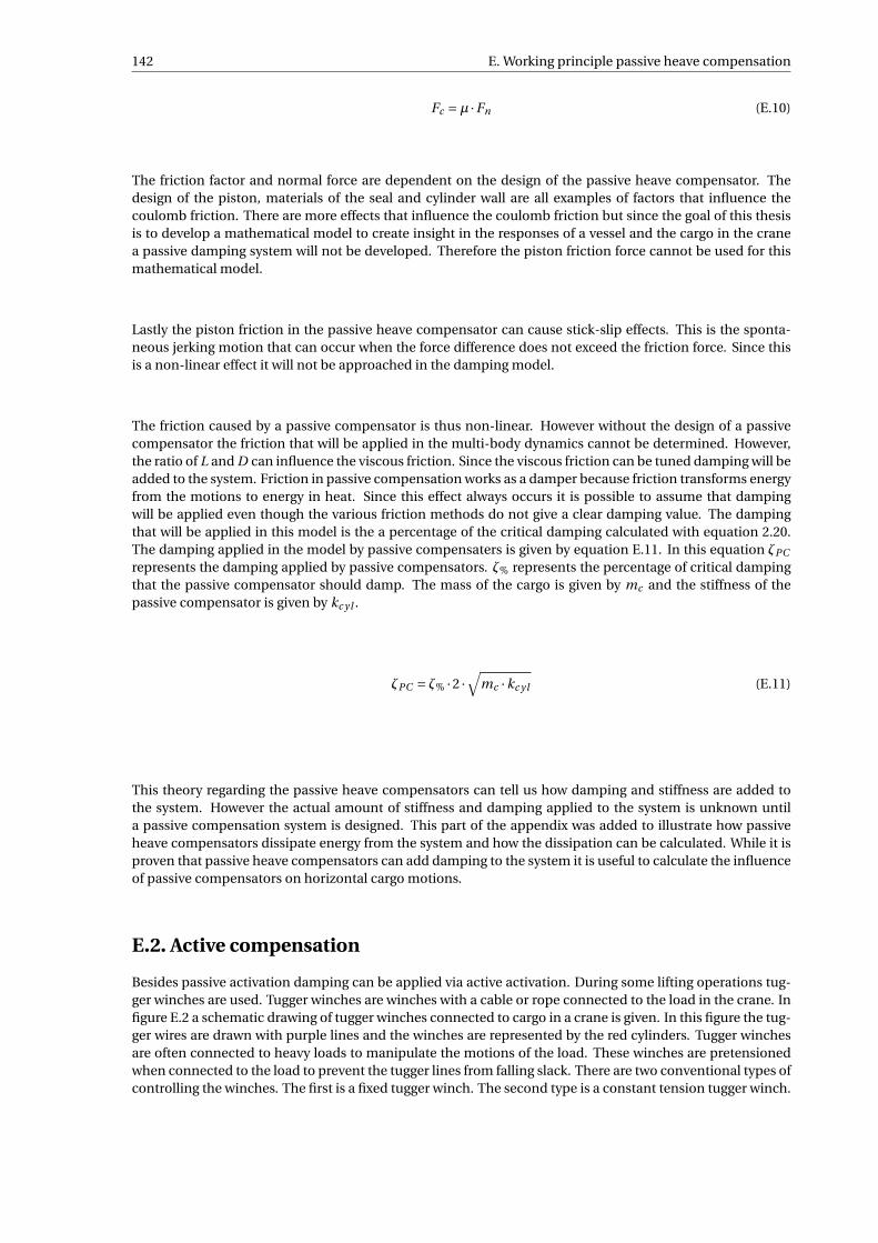
142 E. Working principle passive heave compensation
Fc =µ ·Fn (E.10)
The friction factor and normal force are dependent on the design of the passive heave compensator. Thedesign of the piston, materials of the seal and cylinder wall are all examples of factors that influence thecoulomb friction. There are more effects that influence the coulomb friction but since the goal of this thesisis to develop a mathematical model to create insight in the responses of a vessel and the cargo in the cranea passive damping system will not be developed. Therefore the piston friction force cannot be used for thismathematical model.
Lastly the piston friction in the passive heave compensator can cause stick-slip effects. This is the sponta-neous jerking motion that can occur when the force difference does not exceed the friction force. Since thisis a non-linear effect it will not be approached in the damping model.
The friction caused by a passive compensator is thus non-linear. However without the design of a passivecompensator the friction that will be applied in the multi-body dynamics cannot be determined. However,the ratio of L and D can influence the viscous friction. Since the viscous friction can be tuned damping will beadded to the system. Friction in passive compensation works as a damper because friction transforms energyfrom the motions to energy in heat. Since this effect always occurs it is possible to assume that dampingwill be applied even though the various friction methods do not give a clear damping value. The dampingthat will be applied in this model is the a percentage of the critical damping calculated with equation 2.20.The damping applied in the model by passive compensaters is given by equation E.11. In this equation ζPC
represents the damping applied by passive compensators. ζ% represents the percentage of critical dampingthat the passive compensator should damp. The mass of the cargo is given by mc and the stiffness of thepassive compensator is given by kc yl .
ζPC = ζ% ·2 ·√
mc ·kc yl (E.11)
This theory regarding the passive heave compensators can tell us how damping and stiffness are added tothe system. However the actual amount of stiffness and damping applied to the system is unknown untila passive compensation system is designed. This part of the appendix was added to illustrate how passiveheave compensators dissipate energy from the system and how the dissipation can be calculated. While it isproven that passive heave compensators can add damping to the system it is useful to calculate the influenceof passive compensators on horizontal cargo motions.
E.2. Active compensation
Besides passive activation damping can be applied via active activation. During some lifting operations tug-ger winches are used. Tugger winches are winches with a cable or rope connected to the load in the crane. Infigure E.2 a schematic drawing of tugger winches connected to cargo in a crane is given. In this figure the tug-ger wires are drawn with purple lines and the winches are represented by the red cylinders. Tugger winchesare often connected to heavy loads to manipulate the motions of the load. These winches are pretensionedwhen connected to the load to prevent the tugger lines from falling slack. There are two conventional types ofcontrolling the winches. The first is a fixed tugger winch. The second type is a constant tension tugger winch.

E.2. Active compensation 143
Figure E.2: Schematic drawing of tugger winches applied to cargo in a crane
When the fixed tugger method is used the winches are put on brake when the pretension is finished. The linewill act as a spring in the same way as a mooring line act as a spring on the vessel. The extra stiffness in themulti-body system will influence the natural frequencies of the different degree of freedom. In section 2.6will be explained how stiffness influences the natural frequencies of responses. Since the tugger winches areput on a break this technically is not an active system. In fact, no damping is added via the tugger winchesand fixed tugger lines should be modeled as springs between the location of the winch and the connectionpoint on the cargo. However, the stiffness effects of fixed tugger winches are part of every other system thatintroduces damping. Therefore the fixed tugger winches had to be mentioned and the stiffness componentswill be added when the influence of damping is examined in chapter 6.
A problem with fixed tugger winches is the force applied to the tugger lines. When a load of 500 mton hasa response of 1 meter in horizontal direction on waves with a period of 12 seconds the horizontal dynamicload will be equal to 14 mT. While the waves forces drive the motions of the vessel and cargo system the waveperiod depicts the period of the motions of the multi-body system. This means that a pretension of 14 mTmust be appliled to prevent a slack line. The capacity of the tugger line must be above 28 mT to prevent theline from snapping.
The second method to apply tugger winches to the cargo is a constant tension method. A big advantage ofthe constant tension is the reduced chance of a breaking tugger line. With the constant tension method awinch is set to deliver a constant tension to the tugger lines. When the load of the cargo is moving towardsthe tugger lines the tension in the line reduces and the tugger winch will reel in the tugger line to increasethe tension towards the constant tension value. When the cargo is moving away from the tugger winch thetension in the tugger line increases. This causes the tugger winch to give line to reduce the tension in theline to the constant tension value. When this system is working perfectly the winch will move with the samespeed and phase as the motions of the cargo and there is no tension difference in the line. When there isno tension difference there is no effect of the tugger winches on the dynamic system. Since there is no in-fluence a perfectly working constant tension winch will not influence the responses of the cargo and vesselin a meaningful way. However, in practice the constant tension winches are not perfect. The reaction of the

144 E. Working principle passive heave compensation
winch is always delayed on the motion of the cargo. This causes the tension to fluctuate around the constanttension value. In a complete cycle of the motion a small amount of energy will dissipate from the systemwhich can me modelled as damping. The amount of energy dissipated from the system is hard to model andtherefore impossible to calculate. However small amounts of damping will occur. Therefore, the constanttension winches can be modelled in the same was as a passive compensation system, by applying dampingequal to small percentages of the critical damping. The stiffness of the tugger lines can be calculated in thesame way as the stiffness of the mooring lines explained in section 2.4.
Another active system that might be useful for reducing the cargo motions is an active heave compensationsystem. As in a passive heave compensation system the system is developed to reduce the motions of thecargo in the heave direction. Instead of pneumatics, cylinders and pistons this system uses winches to reducethe motions of the cargo. In figure E.3 a schematic of active heave compensation is given. Since this is anactive system this type of system requires energy input. Instead of a reaction on the forces the motions ofthe vessel are monitored. The motions of the vessel are relayed to a controller. Via the controller an actuatorwill oppose the heave motion. Thus when the vessel has a positive heave motion the controller will force theactuator to move the load in the opposite direction[41]. In figure E.3 the motions of the vessel are opposedby the winch. Such an active system can create possibilities for damping during lifting operations. When theimportant motions of the vessel are monitored an active control system can be put in place. This system couldactively apply damping to the multi-body system. A recently released study from H. Lageveen [15] shows thattugger winches in combination with a controller can be used for active damping. Since it is not in the interestof this study to develop an active damping mechanism no further study to such mechanism is done.
Figure E.3: Schematics of a winch based active heave compensator. For simplicity the crane dynamics is neglected. The stationary
sheave represents the crane tip[[42]
As for the passive compensator systems the active compensator systems do not give actual damping values.However the existence of these systems show that damping can be applied via a system related to active heavecompensation or active tugger winches. This part of the appendix was written to show that there are practicalsolutions to apply damping. Further studies should be done to determine how such a system should look likeand what the specifications of such a system are.