VEIN v0.2.2: an R package for bottom–up vehicular ... · 2Department of Pathology, Faculdade de...

Geosci. Model Dev., 11, 2209–2229, 2018https://doi.org/10.5194/gmd-11-2209-2018© Author(s) 2018. This work is distributed underthe Creative Commons Attribution 4.0 License.

VEIN v0.2.2: an R package for bottom–up vehicularemissions inventoriesSergio Ibarra-Espinosa1, Rita Ynoue1, Shane O’Sullivan2, Edzer Pebesma3, María de Fátima Andrade1, andMauricio Osses4

1Department of Atmospheric Sciences, Universidade de São Paulo, Rua do Matão 1226, São Paulo, SP, Brazil2Department of Pathology, Faculdade de Medicina, Universidade de São Paulo, Av. Dr. Arnaldo 455, São Paulo, SP, Brazil3Institute for Geoinformatics, Westfälische Wilhelms-Universität Münster, Heisenbergstrasse 2, 48149 Münster, Germany4Department of Mechanical Engineering, Universidad Técnica Federico Santa María, Vicuña Mackenna 3939, Santiago, Chile

Correspondence: Sergio Ibarra-Espinosa ([email protected])

Received: 15 August 2017 – Discussion started: 25 September 2017Revised: 3 May 2018 – Accepted: 4 May 2018 – Published: 14 June 2018

Abstract. Emission inventories are the quantification of pol-lutants from different sources. They provide important infor-mation not only for climate and weather studies but also forurban planning and environmental health protection. We de-veloped an open-source model (called Vehicular EmissionsInventory – VEIN v0.2.2) that provides high-resolution ve-hicular emissions inventories for different fields of studies.We focused on vehicular sources at street and hourly levelsdue to the current lack of information about these sources,mainly in developing countries.

The type of emissions covered by VEIN are exhaust (hotand cold) and evaporative considering the deterioration ofthe factors. VEIN also performs speciation and incorpo-rates functions to generate and spatially allocate emissionsdatabases. It allows users to load their own emission factors,but it also provides emission factors from the road transportmodel (Copert), the United States Environmental ProtectionAgency (EPA) and Brazilian databases. The VEIN modelreads, distributes by age of use and extrapolates hourly trafficdata, and it estimates emissions hourly and spatially. Basedon our knowledge, VEIN is the first bottom–up vehicle emis-sions software that allows input to the WRF-Chem model.Therefore, the VEIN model provides an important, easy andfast way of elaborating or analyzing vehicular emissions in-ventories under different scenarios. The VEIN results can beused as an input for atmospheric models, health studies, airquality standardizations and decision making.

1 Introduction

Emissions inventory is a quantification of pollutants dis-charged into the atmosphere by different sources (Pulles andHeslinga, 2010). This quantification is vital for regulatoryand scientific purposes because it allows us to monitor thestate of the Earth’s atmosphere and climate. It also allows usto create air quality standards, which will protect ecosystemsand human health. For instance, the Intergovernmental Panelon Climate Change (IPCC) includes a dedicated task force,separated from the other three working groups, only for thepurpose of greenhouse gas emissions inventory issues (Paus-tian et al., 2006).

In this instance, there are several emissions inventories thatuse different input data and approaches for different scales.One of the most frequently used inventories is the Emis-sion Database for Global Atmospheric Research (EDGAR;Olivier et al., 1996), which provides estimates for the to-tal emissions worldwide. This inventory uses national statis-tics that do not provide detailed characterizations of high-resolution applications. These detailed characterizations areneeded for urban studies. There are also continental emis-sions inventories, such as the European Monitoring and Eval-uation Programme (EMEP), which compile emissions fromthe parties of the Convention on Long-range and Trans-boundary Air Pollution (CLRTAP) (EEA, 2013). Moreover,there is the Regional Emissions inventory in Asia (REAS),which covers China, Japan and other countries (Streets et al.,2003). Also, there are nationwide inventories such as the Na-tional Emissions Inventory (NEI) in the United States, which

Published by Copernicus Publications on behalf of the European Geosciences Union.

2210 S. Ibarra-Espinosa et al.: VEIN v0.2.2

is released every 3 years and is based on data from state, localand tribal agencies and compiled by the Environmental Pro-tection Agency (U.S. EPA, 2018). However, there are manycountries and cities that do not include estimates of emissionsfor environmental and climate planning.

Vehicular emissions are becoming increasingly importantin urban centers (Andrade et al., 2017) and measurementshave shown that compounds emitted from exhausts can behighly reactive in the atmosphere, contributing to criticalepisodes of photochemical smog (Nogueira et al., 2015).However, obtaining this type of emissions database can becomplicated, since the sources are moving and the emissionsprocess is complex with many variables. This can be a chal-lenge, especially in developing countries, due to the lack ofinformation about the vehicle type, technology, age, motorsize, fuel, speeds, accelerations, street type, environmentaltemperature and humidity, among other aspects. Besides that,there are other aspects involving the emissions inventory. Themost common aspects are the accuracy and complexity relat-ing to the exact contribution of the different pollutant sourcesand the fact that, in most cases, emissions inventories are usu-ally seen as a scapegoat when simulations do not match ob-servation (Pulles and Heslinga, 2010).

Vehicular emissions inventories are classified according totop–down and bottom–up approaches. Top–down approachesare based on statistics of vehicle composition, representativespeeds and country balances, while bottom–up approachesare based on traffic counts, vehicle composition and speedrecording (Ntziachristos and Samaras, 2016). An example ofa bottom–up emissions model is the SPARE-Truck (SpatialRegression and Output Optimization Truck) (Perugu et al.,2017), which produces truck activity data at the level ofroad sections between junctions or interchanges (hereafterreferred to as “link”) and then estimates emissions usingthe U.S. EPA MOtor Vehicle Emission Simulator (MOVES)(Koupal et al., 2003). The accuracy of the emissions inven-tory will reflect the representation of the pollutants in the at-mosphere. It is not always related to the complexity of themodel. For instance, a meta-analysis of several studies onvehicular emissions (Smit et al., 2010) concluded that thereis no evidence that the more complex models perform bet-ter than the less complex ones and that emissions estima-tion techniques must be chosen according the available traf-fic data. An emissions inventory must be comprehensive, in-cluding all the important sources and aspects regarding theemissions.

These complexities were addressed by the Department ofAtmospheric Sciences at the University of São Paulo (USP)when modeling the atmospheric chemistry over Braziliancities using a top–down vehicular emissions inventory withan online atmospheric model (Andrade et al., 2015). TheMetropolitan Area of São Paulo (MASP), is the most pop-ulated megacity in Latin America (IBGE, 2014) and its mostimportant source of pollution comes from the 11 million ve-hicles that circulate within the region (CETESB, 2013; DE-

NATRAN, 2015; Andrade et al., 2017). Furthermore, halfof all emissions of carbon monoxide (CO), volatile organiccompounds (VOCs) and nitrogen oxides (NOx) in the MASPare from vehicles that are more than 10 years old (An-drade et al., 2017). Despite the inventories developed by(Andrade et al., 2015) being useful, they still suffer fromtop–down limitations as they use surrogates to produce spa-tial and temporal distributions, hence limiting the represen-tation of the emissions. Therefore, we decided to developour own bottom–up vehicular emissions inventory model.With this model, we aim to generate scientific estimatesand provide useful information to decision makers and ur-ban/environmental planners.

The main goal of this project was to develop a highspatial- and temporal-resolution vehicular emissions inven-tory model, which was named the Vehicular Emissions IN-ventory (VEIN) model. The VEIN model follows a bottom–up approach and includes methods from Ntziachristos andSamaras (2016) and other authors. It is designed for work-ing with and extrapolating outputs of four-stage travel de-mands; however, the model is flexible and could be used witha top–down approach. It allows the classification of vehiclesinto several categories, different options of emission factorsand specification of pollutants, and input traffic from trafficsimulations or other network-based sources. The model in-cludes functions to represent spatial objects and is capable ofproducing gridded emissions outputs. It is open source, user-friendly and available to run in any computational platform(Mac, Windows, Linux, etc.).

2 VEIN model: methodology to estimate vehicularemissions

Temporal and spatial disaggregated emissions are estimatedfollowing a general approach of multiplication between ac-tivities and emission factors (Pulles and Heslinga, 2010), asshown in Eq. (1).

Emissionpollutant =∑

activity

(ARactivity ·EFpollutant, activity

), (1)

where Emissionpollutant for any type of pollutant depends onthe activity rate AR and the emission factors EF, which isthe mass of pollutants generated according to the level of ac-tivity. In the context of vehicular emissions, ARactivity rep-resents the number of vehicles times the distance (km) thatthey travel. EFpollutant, activity is the emission factor (g km−1)for pollutants of the vehicles.

For a bottom–up estimation of vehicular emissions, a largenumber of parameters influence activity (traffic flow, vehiclecomposition, speed recording, length of road) and emissionfactors (speed or acceleration dependent) (Ntziachristos andSamaras, 2016). In this instance, the following sections pro-vide the theory behind the VEIN model regarding traffic data

Geosci. Model Dev., 11, 2209–2229, 2018 www.geosci-model-dev.net/11/2209/2018/

S. Ibarra-Espinosa et al.: VEIN v0.2.2 2211

arrangement, selection of emission factors, emissions estima-tion, spatial allocation and inputs for atmospheric models.

2.1 Traffic data

Traffic data required for the VEIN model must be representedas an hourly amount of vehicles per street.

This traffic data can be provided by traffic simulations, in-terpolations or by other sources. In the first step, VEIN readsspatial morning rush hour traffic data from each street of a de-sired area or city. After reading them, VEIN arranges and or-ganizes the data by vehicle composition, according to Eq. (2).

F ∗i,j,k =Qi ·VCi,j ·Agej,k, (2)

where F ∗i,j,k is the vehicular flow at street link i for vehicletype j by age of use k. j defines the vehicular compositionaccording to their type of use, type of fuel, size of engineand gross weight, based on the definitions of (Corvalán et al.,2002). Qi is the traffic flow at street link i. VCi,j is the frac-tion of vehicles varying according to the type of vehicles j inthe composition for street link i. Agej,k is the age distributionby vehicular composition j and age of use k. This equationshows that VC splits the total vehicular flow Q to identifythe vehicular fraction, which varies according to the type offuel, size of motor and gross weight. For example, if Q islight-duty vehicles (LDVs) and we know that 5 % of the Qare passenger cars (PCs), with an engine of less than 1400 cc,VC is 0.05. This characterization of the fleet depends on theamount and quality of the available information. VEIN thenmultiplies the traffic with age to obtain the amount of eachtype of vehicle by age of use.

Traffic data must be temporally extrapolated because theyare usually available for the morning rush hour. Traffic datacan be estimated from short period traffic count datasets, thenexpanded to represent longer timespan, such as annual aver-age daily traffic (AADT; Wang and Kockelman, 2009; Lamand Xu, 2000). The next step is to extrapolate the vehicularflow at street link i, vehicle type j and age of use k, to ob-tain the vehicular flow for the hour of the week l (Fi,j,k,l ; seeEq. 3).

Fi,j,k,l = F∗

i,j,k ·TFj,l, (3)

where Fi,j,k,l is the traffic flow for each link i and type ofvehicle j of the vehicular composition, with the age of usek for the hour l. TFj,l are the temporal factors varying ac-cording to each hour of l and type of vehicle j . TF is definedas a matrix with 24 lines, and the number of columns repre-sents each day from Monday to Sunday. For instance, if theuser has the output of a travel-demand model for the morn-ing rush hour and also hourly traffic counts, the informationof the hourly traffic count must be arranged to create a ma-trix with 24 lines and with the number of columns to eachday. Then, in order to output the travel-demand model forother hours, TF matrices must be normalized to the hour that

represents the traffic data. This means that TF values for themorning peak hour must be 1 and the respective proportionmust be assigned to the other hours, which is obtained bysimply dividing the traffic of each hour of the matrix by thetraffic of the morning rush hour. TF values can be obtainedfrom automatic traffic count stations or other hourly trafficdata to obtain the temporal profile.

The average speed of traffic flow is very important, and itmust be determined for each link and hour. Once the vehicu-lar flow is identified for each hour, the average speed is thenidentified for each hour. This was accomplished by employ-ing curves from the Bureau of Public Roads (BPR; Bureauof Public Roads, 1964), as shown in Eq. (4). The process in-volves calculating speed by dividing the length of road by thetime. The time is calculated using the total traffic expandedto each street link i and hour l.

Ti,l = Toi ·

(1+α ·

(Qi,l

Ci

)β)(4)

In Eq. (4), Ti is the travel time per street link i at eachhour of the week l. Toi is the travel time under free-flow con-ditions where maximum speed was used. Qi,l is the trafficflow at peak hour for each street link i and hour of the weekl. Ci is the capacity of vehicles on street link i. The parame-ters α and β are adjustments with default values of 0.15 and4, respectively (Bureau of Public Roads, 1964). It has beendescribed that speed decreases as the flow increases until itreaches the capacity of the link, and as the traffic continues toincrease, the speed decreases and travel time increases (Suhet al., 1990). Capacity is the maximum number of vehiclesduring a specific period under prevailing roadway, traffic andcontrol conditions (Manual, 2000). The values of BPR pa-rameters are obtained by regressions of speed and volumetraffic recordings and the default values. The default BPRparameters α 0.15 and β 4 are representative of traffic andcirculation characteristics of the United States. As a conse-quence, other authors have investigated the determination ofcapacity based on local data. For instance, Suh et al. (1990)used Korean data to reestimate α and β by level of service(LOS) A, B, C, D and E, from A (less congested) to E (morecongested), finding values of α= 2.72 and β = 6 for LOS D.In addition, Manzo et al. (2014) estimated the distributionof α and β with Danish data, and Kucharski and Drabicki(2017) found values of α= 0.52 and β = 3.47. Consequently,the user can use different values in the VEIN model insteadof suggested values from the Bureau of Public Roads (1964).This information is important because it allows the user tocalculate the time to travel during link i at any hour l and,therefore, to obtain the speed on that length of the road.

However, the information of the capacity is not alwaysavailable. When information exists at least for the peak andfree-flow speeds, it is possible to apply a simple average ofboth speeds to obtain the average speeds and then distributethese speeds at different hours.

www.geosci-model-dev.net/11/2209/2018/ Geosci. Model Dev., 11, 2209–2229, 2018


2.2 Selection of the emission factors

The emission factors describe the relationship intensity of ac-tivity and emissions for a given technology (Pulles and Hes-linga, 2010). In the case of our model, an emission factor isthe mass of pollutant emitted by the vehicular type, technol-ogy and years of use by traveled distance, as mass of pol-lutant / distance. VEIN takes into account emission factorsfor hot and cold exhaust, evaporative, deterioration and wearemissions. VEIN allows three types of hot exhaust emissionfactors:

1. Speed functions from the COmputer Programme to cal-culate Emissions from Road Transport (Copert; Ntzi-achristos and Samaras, 2016), which are stored inter-nally in the model. This approach can be used if thereis no local emission factors and if there is informationabout vehicular speed recordings, simulations or knowl-edge of the representative speeds.

2. Emission factors from local sources. The values must bemass per kilometer (g km−1) per specific type of vehi-cle, including fuel type, size and weight by age of use.For instance, Brazilian emission factors in the officialemissions inventory report are averaged emissions ofannual emission certification tests by type of vehicle,fuel type, size and weight (CETESB, 2013), and theyare not speed functions. Nevertheless, this capabilitycan be utilized with different types of emission factorssuch as tunnel studies or dynamometer measurementswhich are not speed functions. Appendix B shows anexample of VEIN being used with different emissionfactors.

3. Scaled local emission factors with Copert in order toincorporate speed variation for local factors, as shownin Eq. (5). This produces a specific speed dependenceon emission factor by age of use for the vehicle.

Copert emission factors are based on emission measurementsmade in Europe. This means that there is an inherent fuelcomposition associated with these factors. When the user in-tends to use these factors, they must be corrected with thelocal fuel properties as shown by Ntziachristos and Samaras(2016). However, if the user uses emission factors based onlocal measurements, this correction is not necessary.

EFscaled(Vi,l)j,k,m = EF(Vi,l)j,k,m ·EFlocalj,k,m

EF(Vdci,l)j,k,m, (5)

where EFscaled(Vi,l)j,k,m is the scaled emission factor andEF(Vi,l)j,k,m is the Copert emission factor for each streetlink i, vehicle from composition k, hour l and pollutantm. EFlocalj,k,m represents the constant emission factor (notspeed functions). EF(Vdci,l)j,k,m are Copert emission fac-tors with average speed value of the respective driving cyclefor the vehicular category j . The São Paulo emission fac-tors data include recordings of the Federal Test Procedure

(FTP-75) driving cycle for LDV with an average speed of34.12 km h−1, as shown in the report of driving cycles (Bar-low et al., 2009).

By default, VEIN includes a deterioration factor fromCopert (Ntziachristos and Samaras, 2016). This deteriorationfactor depends on accumulated mileage and technology asso-ciated with Euro standards on vehicles with three-way cata-lysts. However, it is possible to include other sources, suchas from Corvalán and Vargas (2003).

2.3 Emissions estimation

VEIN estimates type of emissions including hot exhaust(EH; Eq. 6), cold-start exhaust (EC; Eq. 7), evaporative (EV;Eq. 8), deterioration factors and speciation. The total vehicu-lar emission is the sum of all types of emissions.

2.3.1 Hot exhaust emission

The VEIN process of emissions estimation is performed perstreet link, vehicle type, hour of week and pollutant. Equa-tion (6) shows the hot exhaust estimation:

EHi,j,k,l,m = Fi,j,k,l ·Li ·EF(Vi,l)j,k,m ·DFj,k. (6)

In Eq. (6), EHi,j,k,l,m is the emissions for each street link i,vehicle category from composition k, hour l and pollutantm,where Fi,j,k,l is the vehicular flow calculated in Eq. (1). Liis the length of the street link i. EF(Vi,l)j,k,m is the emissionfactor of each pollutant m. DFj,k is the deterioration factorfor vehicle of type j and age of use k. Deterioration factorsare emission degradation functions of gasoline vehicles us-ing catalysts due to accumulated mileage based on Europeanmeasurements (Ntziachristos and Samaras, 2016). Neverthe-less, the users could use their own set of deterioration factorssuch as that proposed by Corvalán et al. (2002).

2.3.2 Cold-start emissions

Cold-start emissions are produced during engine startup,when the engine and/or catalytic converter system has notreached its normal operational temperature. Consequently,these emissions occur when a vehicle starts its journey at theparking location or mostly in residential streets. Several stud-ies have shown the significant impact of these types of emis-sions (Chen et al., 2011; Weilenmann et al., 2009). VEINalso considers cold-start emissions – under this condition,emissions will be higher, and if the atmospheric tempera-ture decreases, cold-start emissions will increase regardlessof whether the catalyst has reached its optimum tempera-ture for functioning (Boulter, 1997). For example, Ludykaret al. (1999) measured vehicular emissions with the Euro-pean driving cycle (EDC) at 22, −7 and −20 ◦C, finding thatat lower temperatures, CO increased 5 times, NOx 1 time,hydrocarbons (HC) 14 times and particulate matter (PM)46 times, but specific hydrocarbons increased more, such



as Toluene, which increased 21 times, and PAH, which in-creased 33 times.

The VEIN model caters to these emissions by using the ap-proach outlined in Copert (Ntziachristos and Samaras, 2016),as shown in Eq. (7).

ECi,j,k,l,m = βj ·Fi,j,k,l ·Li ·EF(Vi,l)j,k,m ·DFj.k·(EFcold(tan,Vi,l)j,k,m− 1

)(7)

This approach adds two terms to Eq. (6). The first termEFcold (tan,Vi,l)j,k,m −1 is the emission factors for cold-start conditions at each street link i, vehicle category fromcomposition k, hour l, pollutantm and monthly average tem-perature n. Ntziachristos and Samaras (2016) suggest usingmonthly average temperature. As the information about theparking locations is limited, in Eq. (7) we propose assign-ing the emissions by links. In cases when better informationis available, these emissions should be assigned into parkinglocations.

The second term βj is defined as the fraction of mileagedriven with a cold engine/catalyst (Ntziachristos and Sama-ras, 2016). The VEIN model incorporates a dataset of coldstarts recorded during the implementation of the Interna-tional Vehicle Emissions (IVE) model (Davis et al., 2005)in São Paulo (Lents et al., 2004), which provides the hourlymileage driven with cold-start conditions. The data of startpatterns should be generated by each user with local data. Forinstance González et al. (2017) generated a start pattern us-ing surveys to estimate vehicular emissions with IVE. How-ever, the user eventually could use the start pattern availablein VEIN only in the absence of other data. Alternatively, theuser could follow the Ntziachristos and Samaras (2016) forestimating β, which consists in β = 0.6474− 0.02545 ∗ ltrip− (0.00974− 0.000385 ∗ ltrip) ∗ ta, where ltrip is the averagelength of the trip and ta is the average monthly temperature.

2.3.3 Evaporative emissions

Evaporative emissions are important sources of hydrocar-bons, and these emissions are produced by vaporization offuel due to variations in ambient temperatures (Mellios andNtziachristos, 2016; Andrade et al., 2017). There are mainlythree types of evaporative emissions: diurnal emissions, dueto increases in atmospheric temperature, which lead to ther-mal expansion of vapor fuel inside the tank; running losses,when the fuel evaporates inside the tank due to normal op-eration of the vehicle; and hot-soak emissions, which occurwhen the hot engine is turned off. These methods imple-mented in VEIN were sourced from the evaporative emis-sions methods of Copert (Mellios and Ntziachristos, 2016).This approach is shown in Eqs. (8), (9) and (10).

EVj,k =∑

sDs ·

∑j

Fj · (HSj,k + dej,k +RLj,k), (8)

where EVj is the volatile organic compound (VOC) evap-orative emissions due to each type of vehicle j . Ds is the

“seasonal days” or number of days when the mean monthlytemperature is within a determined range: [−5◦, 10 ◦C], [0◦,15 ◦C], [10◦, 25 ◦C] and [20◦, 35 ◦C]. Fj,k is the number ofvehicles with to the same type j and age of use k. HSj,k , dej,kand RLj,k are average hot/warm-soak, diurnal and runningloss evaporative emissions (g day−1), respectively, accordingto the vehicle type j and age of use k. HSj,k and RLj,k areobtained using equations also sourced from

HSj,k = xj,k ·(c ·(p ·eshc+(1−p) ·eswc)+(1−c) ·eshfi), (9)

where x is the number of trips per day for the vehiculartype j and age of use k. c is the fraction of vehicles withfuel return systems. p is the fraction of trips finished with ahot engine, for example, an engine that has reached its nor-mal operating temperature and the catalyst has reached itslight-off temperature (Ntziachristos and Samaras, 2016). Thelight-off temperature is the temperature at the point when cat-alytic reactions occur inside a catalytic converter. eshc andeswc are average hot-soak and warm-soak emission factorsfor gasoline vehicles with carburettor or fuel return systems(g parking−1). eshfi is the average hot-soak emission factorsfor gasoline vehicles equipped with fuel injection and non-return fuel systems (g parking−1).

RLj,k = xj,k ·(c ·(p ·erhc+(1−p) ·erwc)+(1−c) ·erhfi) (10)

x and p have the same meanings as in Eq. (9). erhc anderwc are average hot and warm running loss emission factorsfor gasoline vehicles with carburettor or fuel return systems(g trip−1), and erhfi is the average hot running loss emissionfactors for gasoline vehicles equipped with fuel injection andnon-return fuel systems (g trip−1). It is recommended to esti-mate the number of trips per day (Mellios and Ntziachristos,2016), x, as the division between the mileage and 365 times

the length of trip: x =mileagej(365 · ltrip)

. However, the mileage of

a vehicle is not constant over the years. Therefore, VEINincorporates a dataset of equations to estimate mileage ofdifferent types of vehicles by age of use (Bruni and Bales,2013). The methods presented in this part correspond to theevaporative emission factors Tier 2 (Mellios and Ntziachris-tos, 2016). However, we expect to add Tier 3 methods in fu-ture versions of VEIN, including hourly distribution parkingpatterns. Alternatively, for convenience, the user could trans-form the units to produce emission factors in grams per kilo-meter for convenience. For instance, in Eqs. (9) and (10), xis the number of trips per day, knowing that the mean dis-tance per trip would allow x to be calculated as the distancetraveled per day.

2.4 Speciation of emissions in chemical subcomponents

Particulate matter and hydrocarbons are a mixture of sev-eral chemical compounds that play an important role in at-mospheric chemistry (Seinfeld and Pandis, 2016). VEIN in-cludes speciation profiles for hydrocarbons and particulate



matter from Ntziachristos and Samaras (2016) and Ibarra(2017). These profiles are percentages of the emissions byvehicle type, fuel, emission standard and other characteris-tics. Speciations are also included for particulate matter inblack carbon and organic matter; particulate matter fractionsfor tire, brake and road wear; non-methanic hydrocarbons(NMHC); and nitrogen oxides. In this case, the NMHC spe-ciations from Ibarra (2017) cover emissions from vehiclesconsuming gasohol (gasoline with 25 % of ethanol), ethanoland diesel from exhaust, evaporative and liquid fuel releasedto the atmosphere. This speciation is based on measure-ments made in Brazil during the studies of Rafee (2015),Ynoue (2004), Albuquerque (2005), Oliveira (2007), Mi-randa (2001), Vara-Vela et al. (2016) and Andrade et al.(2015). Hence, it is advisable that users from other na-tions/locations use suitable data for their local conditions.

2.5 Spatial allocation and databases

VEIN provides functions to generate grids and spatially al-locate emissions into grids. This is helpful for the visualiza-tion and generation of inputs for atmospheric models and asa tool for urban planning. In addition, VEIN includes func-tions to produce a database of hourly emissions for vehicularcomposition by age of use. Section 4.4 provides details andexamples about the emissions grids and databases.

3 VEIN model design

The VEIN model was constructed using the free open-sourceR software (R Core Team, 2017). R is a programming lan-guage and environment for statistical computing and graph-ics (R Core Team, 2017). It was developed primarily for an-alyzing data. However, since its capabilities have grown overtime, R has become a flexible language with many differ-ent areas of application. It includes elements of programminglanguages such as Lisp and the syntax of S, as described byLeiner et al. (1997).

The VEIN R package depends on the package “sp” (Bi-vand et al., 2013), as it uses several of its classes. VEIN im-ports some functions from the package “rgeos” (Bivand andRundel, 2016), which is an interface for the Geometry open-source (GEOS) library (https://trac.osgeo.org/geos/, last ac-cess: 31 May 2018). It also imports functions from “rgdal”(Bivand et al., 2016), which provides bindings to the Geospa-tial Data Abstraction Library (GDAL; http://www.gdal.org/,last access: 31 May 2018). Therefore, these R packages mustbe installed prior to using the VEIN package.

VEIN started between 2014 and 2016 as a collectionof several R scripts, initially named R-EMIssions (REMI;Ibarra-Espinosa and Ynoue, 2017), which later evolved intoan R package. It was developed in R due to the free open-source advantages and because R allows easier reproducibil-ity. VEIN is open to scrutiny from its community of users,

thus allowing opportunities for user feedback and improve-ments. This facilitates widespread use of the model and iden-tifying any software bugs/errors, with the potential for addingnew capabilities. VEIN has its own functions, but it also in-corporates other data and functions such as emission factorsand mileage.

VEIN can be installed from the Comprehensive RArchive Network (CRAN; https://CRAN.R-project.org/package=vein, last access: 31 May 2018) or from the web-site Github (https://github.com/atmoschem/vein). In order touse the VEIN library and run the demo, it is necessary to runthe following scripts in R:

install.packages("vein") #orlibrary(devtools)install_github("atmoschem/vein")library(vein)demo(VEIN)

The diagram process for estimating emissions is shown inFig. 1. The circles in this figure refer to the data and the boxesrefer to the functions inside the model. The VEIN modeldiagram starts at the circle for traffic, which represents themorning rush hour traffic data for each street link. Then the“age” functions (“age_ldv”, “age_hdv” or “my_ldv”) deter-mine the vehicular composition by age of use as shown inEq. (2). The data “profile” allows us to temporally extrapo-late traffic data to the other hours, and this allows us to esti-mate the average vehicular speed at any hour and link usingthe function “netspeed”. Emission factor selections start byadding the deterioration effect with the function “emis_det”to local, speed-dependent emission factors from Ntziachris-tos and Samaras (2016), denoted as “speed_ef”, or scaledemission factors, denoted as scaled_ef in Fig. 1. Besidesincluding speed-dependent emission factors from Ntziachris-tos and Samaras (2016), VEIN also includes local emissionfactors from CETESB (2016). Once the input data are ready,the function “emis” estimates hourly emissions for each hourof the day and day of the week. The function “emis_post”produces an emissions database by vehicle category or bystreet, denoted as “df” and “street” in Fig. 1, respectively.These emissions are then speciated with the function “speci-ate”. At this time, the user can create a grid with the function“make_grid”, which creates a rectangular spatial grid withformat SpatialPolygonsDataFrame used to allocateemissions spatially with the function “emis_grid”. The func-tion “emis_wrf” reads the emissions grids and creates a dataframe ready to be used with the NCL script AS4WRF (Vara-Vela et al., 2016), which creates an input for the WRF-Chemmodel (Grell et al., 2005). The user can also use the modeleixport (Ibarra-Espinosa et al., 2018) to create inputs for themodel WRF-Chem or BRAMS (Freitas et al., 2005) usingonly R (R Core Team, 2017).


https://trac.osgeo.org/geos/

http://www.gdal.org/

https://CRAN.R-project.org/package=vein



Figure 1. Representation of the VEIN model. Boxes and circles represent functions and data, respectively.

3.1 Functions and classes

VEIN uses objects of the class “Spatial” (Pebesma and Bi-vand, 2005), including SpatialLinesDataFrame. Toread geospatial data, there are several packages, such as rgdal(Bivand et al., 2016) or “maptools” (Bivand and Lewin-Koh,2015). The main requirement is that the network must be aSpatialLinesDataFrame, a class of sp (Pebesma andBivand, 2005).

We included several functions to arrange traffic data, se-lect or scale emission factors, as well as estimate and processemissions in VEIN, as shown in Table 1. These functions im-plement the equations shown in Sect. 2.

VEIN incorporates eight classes (see Table 1), which areobjects with specific characteristics: methods and units. Themethods are print, summary and plot. They are functions thatreturn a specific result depending on each class. Another im-portant characteristic of each class is that they include ex-plicit units, in an effort to reduce human error and improveusability. For this task, VEIN imports some functions of thepackage “units” (Pebesma et al., 2016), which is an inter-face in the C library “udunits” from University Corporationfor Atmospheric Research (UCAR). Therefore, this librarymust be installed on the system prior to using VEIN. Onlythe EmissionFactorsList and EmissionsArraydo not show their units explicitly due to limitations with theunits package. The classes outlined in Table 1 are also con-structor functions, which means that they can create VEINclasses and add the respective units. VEIN incorporate con-structor functions to create classes such as Vehicles orEmissions. These functions are incorporated inside otherVEIN functions in order for the output of VEIN to have aclass. When the constructor functions are applied to a nu-meric element, the constructor simply adds the units and theresulting object has class units. For example, applying thefunction EmissionsArray to a numeric vector will addthe units grams per hour to the numeric vector.

4 Estimating MASP vehicular emissions using VEINmodel

This section presents the application of the most importantfunctions of the VEIN model. These functions obtain an es-timate of CO emissions from LDV fleets in MASP for 2015(for a typical non-holiday week).

4.1 Traffic data for MASP

Hourly traffic is a requirement for these data. These data canonly be represented as 1 h of data, which can then be ex-trapolated with the VEIN functions or as a list of hourlytraffic data for all the covered hours. The present applica-tion includes a four-stage travel-demand model for MASPCET (2014) for a morning rush hour loaded into R as aSpatialLinesDataFrame. It includes peak and free-flow speeds, along with capacity (maximum amount of ve-hicles that can circulate in a road per hour) and trafficflow from LDV and HDVs (heavy-duty vehicles). Figure 2shows the traffic simulation of LDV at 08:00–09:00 localtime (LT), where urban motorways concentrate the highestamount of vehicles. The total volume of LDV is 24 708 767veh h−1 and the number of streets are 34 733, with a meanof 711 veh h−1 street−1. It is important to note that the VEINmodel provides an extraction of the traffic simulation for thewestern part of São Paulo. The traffic simulation for MASPhas a size of 61.6 Mb and the extraction for the western partof São Paulo 3.1 Mb. We provided the extraction and not thewhole traffic simulation in VEIN to make it faster. This sec-tion provides codes to run VEIN so that the reader can followthem with the data provided in the model.

After loading traffic data, the traffic flow was expandedto each hour of the week with the function “temp_fact”, asshown in the following scripts. It is also necessary to ex-trapolate hourly vehicle speeds. Therefore, we created thefunction netspeed, which applies the function BPR (Bureauof Public Roads, 1964) curves, according to Eq. (4). To use



Table 1. Summary of the VEIN classes, functions and internal data.

Function Description Reference

age_hdv Distribution of HDV by age of use Ministério do Meio Ambiente (2011)age_ldv Distribution of LDV by age of use Ministério do Meio Ambiente (2011)age_moto Distribution of motorcycle by age of use Ministério do Meio Ambiente (2011)ef_evap Evaporative emission factors Mellios and Ntziachristos (2016)ef_hdv_scaled List of scaled emission factors for HDV Ntziachristos and Samaras (2016)ef_hdv_speed HDV emission factors Ntziachristos and Samaras (2016)ef_ldv_cold LDV cold-start emission factors Ntziachristos and Samaras (2016)ef_ldv_cold_list List of LDV cold-start emission factors Ntziachristos and Samaras (2016)ef_ldv_scaled List of scaled emission factors for LDV Ntziachristos and Samaras (2016)ef_ldv_speed LDV emission factors Ntziachristos and Samaras (2016)ef_wear Tire and brake wear, road abrassion Ntziachristos and Boulter (2009)EmissionFactors Creates class EmissionFactors (g km−1)EmissionFactorsList Creates class EmissionFactorsList (g km−1)Emissions Creates class Emissions (g h−1)EmissionsArray Creates class EmissionsArray (g h−1)EmissionsList Creates class EmissionsList (g h−1)emis Estimation to hour and day of the weekemis_cold Cold-start estimation Ntziachristos and Samaras (2016)emis_det Deterioration factors Ntziachristos and Samaras (2016)emis_evap Evaporative estimation Mellios and Ntziachristos (2016)emis_grid Allocation on rectangular gridemis_paved Resuspension of paved roads U.S. EPA (2016)emis_post Post-processing of emissionsemis_wear Estimation of wear emissions Ntziachristos and Boulter (2009)emis_wrf Creating data frame to NCL AS4WRF Vara-Vela et al. (2016)Evaporative Creates class Evaporative (g ·d−1)fe2015 Data of CETESB emission factors CETESB (2016)fkm Data of mileage functions by vehicle Bruni and Bales (2013)hot_soak Hot-soak evaporative Mellios and Ntziachristos (2016)make_grid Rectangular gridmy_age Distribution of vehicles by age of usenet Data of traffic simulation of west São Paulo CET (2014)netspeed Estimate average speedpc_profile Data of temporal factors ARTESP (2012)pc_cold Data of vehicle start pattern Lents et al. (2004)running_losses Evaporative estimation Mellios and Ntziachristos (2016)speciate Split by species Ntziachristos and Samaras (2016),

Ibarra (2017)Speed Creates class Speed (km h−1)temp_fact Expand hourly trafficVehicles Creates class Vehicles (1 h−1)vkm Determination of vehicle kilometers

BPR, a data frame is required with total traffic at all hoursand the morning rush parameters capacity, peak speed, free-flow speed and length of the road and with the BPR parame-ters alpha and beta. The argument “scheme” produces a 24 hspeed data frame, based only on peak and free-flow speedwith a profile of free-flow speeds in the early mornings, peakspeeds, and morning and evening rush hours and the averageat hours in between. If the time lapse for the emissions esti-mation is longer than a week, the user could simply replicatethe hours until it reaches the desired hours.

data(net)data(pc_profile)pcw <- temp_fact(net$ldv+net$hdv,pc_profile)speed <- netspeed(pcw, net$ps, net$ffs,net$capacity, net$lkm, alpha = 1)

To illustrate this, the resulting speeds are observed inFig. 3, which shows two different speed maps: one for08:00 LT (panel a) and the other for 23:00 LT (panel b). This



Figure 2. Traffic flow simulation for LDV (veh h−1) at 08:00–09:00 LT for MASP.

figure shows that the highest speeds are found in most ofthe streets further away from the MASP center at both times(08:00 and 23:00 LT). The major difference between the twopanels (a and b), is that late at night, the flow is faster nearthe center of MASP. This seems reasonable since the vehic-ular flow tends to diminish during the night. The averagespeeds also show a pattern related to the type of street asshown in Fig. 4. The type of street comes form São Paulotraffic simulation; the names of the different types were trans-lated into English and are as follows. Motorway: roads withspeed limits above 80 km h−1 without physical intersections.Arterial: roads with a speed limit of 60 km h−1 with inter-sections such as traffic lights. Collector: roads with a speedlimit of 40 km h−1 that collect and distribute traffic betweenarterial roads. Local: roads with a speed limit of 30 km h−1

that access restricted zones. Figure 4 shows that lower speedsare found during the morning (07:00–10:00 LT) and evening(17:00–20:00 LT) rush hours. This is important in terms ofair pollution because at lower speeds vehicles emit more pol-lutants (Ntziachristos and Samaras, 2016). By contrast, max-imum average speeds for each type of road are obtained dur-ing night hours and on Sundays at all hours.

After calculating the São Paulo traffic flow average speedsfor each hour of the week and each street link, the age dis-tribution of the fleet was obtained by type of vehicle. The“age*” functions (age_ldv, age_hdv and “age_moto”) dis-tribute the traffic data by the vehicle’s age of use. These func-tions return a data frame with the number of rows matchingthe number of streets, columns representing the amount ofvehicles by age of use and a message indicating the averageage of the fleet. The age* functions are related to Eq. (2),where they split the vehicular flow at street link Qi by typeof vehicle j and the vehicle’s age of use k. These functionsare based on the survival equations presented in the Brazil-ian Emissions Inventory Report by the Ministério do MeioAmbiente (2011) and are parameterized for the VEIN model.

They allow the use of different coefficients to obtain differ-ent age distributions allowing the representation of differentrealities. Furthermore, the function “my_age” distributes thetraffic from an existing dataset, e.g., yearly vehicle licensing.

The following code shows three uses of age* functions.The first, my_age, uses yearly traffic data from the reportof the São Paulo emissions inventory (CETESB, 2016), ex-pressed as CETESB_PC based on vehicle sales. The second,age_ldv, uses default parameters, and the third, age_ldv, usesb=−0.14.

CETESB_PC <- c(33491,22340,24818,31808,46458,28574, 24856,28972,37818,49050,87923,133833, 138441,142682,171029,151048,

115228,98664, 126444,101027,84771,55864,36306,21079, 20138,17439,7854,2215,656,1262,476,512, 1181,4991,3711, 5653, 7039,

5839, 4257, 3824,3068)

pc1 <- my_age(x = net$ldv,y = CETESB_PC, name = "PC")pc2 <- age_ldv(x = net$ldv,name = "PC", agemax = 41)pc3 <- age_ldv(x = net$ldv,name = "PC", b = - 0.14, agemax = 41)

Figure 5a shows three age distributions, each one has24 708 767 veh h−1, and each has a different average age.Each curve represents the São Paulo LDV fleet according toits age of use, with an estimated average age of 11.09 years(red line), 15.53 years (blue line) and 15.17 years (greenline). This figure shows that in MASP there are more newervehicles than older ones. age* functions also include a log-ical option named “bystreet”, with a default value equal toFALSE. When this value is TRUE, age* expects that the co-efficients a and b for the age* functions are numeric vec-tors, with length matching the number of streets. This al-lows different age distributions within the same road net-work, and this is particularly useful for areas with less in-formation about the vehicles’ age of use.

4.2 Emission factors

Once we obtain the traffic flow for the desired type of vehi-cles (in our LDV example), for each hour of the day, for all(desired) days of the week, for each age distribution and foreach street link, then we can proceed to the emissions calcu-lation itself.

The VEIN package includes a database entitled “fe2015”with emission factors for PC and light trucks by age ofuse from the São Paulo official vehicular emissions inven-tory (CETESB, 2016). This inventory was compiled using atop–down approach, and the pollutants estimated were CH4,CO, CO2, HC, N2O, NMHC, NOx and PM. These data in-



Figure 3. Traffic speeds (colored lines; km h−1) for LDV fleet at 08:00 LT (a) and 23:00 LT (b) in MASP.

Figure 4. Traffic average speeds for LDV fleet by type of street (colored lines) at 08:00–09:00 LT in MASP.

clude national and equivalent Euro emission standards byyear and age. The equivalence among Brazilian CONAMA(1986), MMA (2011), MMA (2015) and the Euro Direc-tive70/220/EEC (1991) was added to this database in orderto choose the corresponding matching vehicle and emissionsstandard. The equivalence can be seen in Table 2.

fe2015 emission factors do not include the deteriorationeffect due to the accumulated age of vehicles, and it must beincluded. This is done with the deterioration factor functionemis_det, which has the arguments pollutant, size of engine,Euro standard and mileage in kilometers. VEIN includes aBrazilian database of mileage functions named “fkm”, whichis a list of functions with each element of the list corre-sponding to vehicle type. These functions depend on thevehicle’s age of use, and they originate from the odometerreadings of more than 1.6 · 106 vehicles (Bruni and Bales,2013). emis_det includes deterioration factors from Ntzi-achristos and Samaras (2016), which are based on measure-ments of European vehicles consuming gasoline; however,most of Brazilian automotive fuel sold has a mixture of bio-fuels such as ethanol from sugarcane. To our knowledge,there are no published deterioration factors for Brazilian con-ditions. Hence, we believe that including deterioration fac-tors from Ntziachristos and Samaras (2016) is a valid optionin the absence of better data. Another aspect that it is impor-

Table 2. Proposed equivalence of emission standards used in SãoPaulo study.

Brazilian EuroVehicle standard standard Year

LDV

L – 1 Pre Euro 1988–1991L – 2 Euro 1 1992–1996L – 3 Euro 2 1997–2004L – 4 Euro 3 2005–2011L – 5 Euro 4 2012–2013L – 6 Euro 5 2014

HDV

P – 1 Pre Euro 1990–1992P – 2 Pre Euro 1993P – 3 Euro 1 1994–1997P – 4 Euro 2 1998–2003P – 5 Euro 3 2004–2011P – 6 Euro 4 –P – 7 Euro 5 2012

MotorcycleM – 1 Euro 1 2003–2005M – 2 Euro 2 2006–2008M – 3 Euro 3 2009

Based on https://www.transportpolicy.net/standard/brazil-light-duty-emissions/, lastaccess: 31 May 2018.


https://www.transportpolicy.net/standard/brazil-light-duty-emissions/

https://www.transportpolicy.net/standard/brazil-light-duty-emissions/


tant to mention is that, when improved fuels are consumedin an older fleet, for instance fuel designed for Euro III tech-nology in a pre-Euro fleet, this will diminish the emissions inolder fleet. This fuel effect it is being included in the devel-opment repository of VEIN.

Emission factors for PCs, light commercial vehicles(LCVs) and motorcycles are called with the function“ef_ldv_speed”. In the case of trucks and buses, the func-tion “ef_hdv_speed” is used. The arguments are filters for aninternal database of emission factors which include severalparameters such as fuel, Euro standard, volume of engine andload, among others. These functions also include a multipli-cation factor with a default value of 1. Exact spelling is re-quired when using the arguments. If the argument names areentered incorrectly, VEIN will not return the emission factorfunctions.

The following code shows how to read the emission factorsof the VEIN databases fe2015, “pc_profile” and fkm, in or-der to incorporate the deterioration effect into the CETESB(2016) emission factors. The age of LDV shown in Fig. 5ahas a length of 41 years. This means that it needs 41 emis-sion factors, one per each age of use. We used a 41-year dis-tribution because we want to have a realistic representationof the vehicles in circulation by age of use, despite the old-est vehicles having a small number. However, the user coulduse a different age distribution, such as 50 years. This al-low us to obtain emissions by the age of use of the vehicles;hence, VEIN can be used as a fast tool for scrapping poli-cies and other applications. It calls the function emis_det,which requires the accumulated mileage, obtained from thelist of mileage equations fkm. Fig. 5c)shows the emissionfactors from CETESB with and without deterioration by ageof use. We are using deterioration factors from Ntziachris-tos and Samaras (2016) that affect only vehicles with a cat-alytic system. The base year of this emissions estimation is2015, and vehicles with catalytic systems started in 1992 inBrazil (23 years before 2015). Therefore, the vehicles thatentered the market before 1992 do not include deterioration.The emission factors dataset fe2015 includes emission fac-tors for vehicles with only 36 years of use, but the vehiculardistribution calculated in the last script has 41 years of use.Therefore, we repeated the oldest emission factors to have41 emission factors. Here we are assuming that the emissionfactors of vehicles with 36 years of use are the same as forthe vehicles with 41 years of use. The last line of the fol-lowing script calculates the deteriorated emission factors ofpassenger cars by age of use.

data(fe2015)data(fkm)pckm <- fkm[[1]](1:24)pckma <- cumsum(pckm)cod1 <- emis_det(po = "CO", cc = 1000,eu = "III", km = pckma[1:11])cod2 <- emis_det(po = "CO", cc = 1000,

eu = "I", km = pckma[12:24])co1 <- fe2015[fe2015$Pollutant == "CO", ]

co1[37:41, ] <- co1[36, ]cod <- c(co1$PC_G[1:24] * c(cod1, cod2),co1$PC_G[25:nrow(co1)])

Once the deterioration effect was added to the Brazilianemission factors (CETESB, 2016), they were scaled to ac-count for speed with the function “ef_ldv_scaled”. This func-tion is used to multiply emission factors from ef_ldv_speedwith a constant.

The new emission factor (dependent on speed) has thesame value as the local emission factor, which is evaluatedat the reference speed of the measurement 34.12 km h−1 forFTP-75. The default speed value is 34.12 km h−1, but thisvalue must change correspondingly to the speed of the driv-ing conditions. To use this function, it is necessary to scaleemission standards of local emission factors with Euro stan-dards. In the following code, “Euro_LDV” is a vector indi-cating Euro standard by age of use.

lef <- ef_ldv_scaled(co1, cod, v = "PC",cc = "<=1400", f = "G", p = "CO",eu = co1$Euro_LDV)

4.3 Emission estimation

After inputting the database of vehicles and their respectiveemission factors, VEIN is ready to use the emis function. TheVEIN package uses several emis functions according to thetype of emission being estimated. The emis function assem-bles data and outputs from other VEIN functions and esti-mates the emissions for the number of hours and days in theweek. This function reads the morning rush hour traffic databy age of vehicle use and extrapolates it with the profile dataframe, as previously explained. It reads the emission factorsstored in a list with length matching the age distribution ofthe vehicle category and then reads the list of speeds. Thisfunction returns the emissions at each street in an array withfour dimensions: (1) number of streets; (2) maximum age ofage distribution; (3) hours (usually 24); and (4) days (usually7). For convenience, there are defined default values for thisfunction: hour – 24; day – 7; array – TRUE. The values canbe changed as necessary.

For example, the estimation of the traffic simulationsshown in Fig. 2 has 34 733 streets, a fleet with a 41-year agedistribution, 24 h of the day, and 7 days of the week. There-fore, it will produce an emissions array with the dimensions34 733, 41, 24 and 7. The vehicle fleet used to produce theage distribution is shown in green in Fig. 5a, and it is 41 yearsin length.

E_CO <- emis(veh = pc1, lkm = net$lkm,ef = lef, speed = speed,profile = pc_profile)



Figure 5. (a) Distribution of LDV composition by age of use, (b) temporal factor for expanding morning rush hour traffic data and (c) COemission factors used in the estimation presented in this paper.

This emissions array output for 34 733 streets and a vehi-cle fleet with a 41-year age distribution, 24 h and 7 days ofthe week, has the size of 1.8 Gb. Hence, it is recommended touse the function emis_post and then delete the original emis-sions array. The arguments include the emissions array, typeof vehicle, size or weight, fuel, pollutant, and the boolean ar-gument “by”. The emis_post function was created to preservethe most important information in the emissions array, to useless memory size and to be compatible with the packagessp (Pebesma and Bivand, 2005) and “ggplot2” (Wickham,2009). VEIN outputs could also be used with the package“openair” (Carslaw and Ropkins, 2012). emis_post returns adata frame, but the argument by determines the shape of thedata frame. When by has the value “veh”, it returns a dataframe with an aggregation of the emissions array by each ve-hicle’s age of use with the following columns: vehicle name,emission (in grams), vehicle type, size, fuel, pollutant, age,hour and day. This output allows the user to visualize hourlyemissions at each day of the week, as shown in Fig. 6. Higheremissions are found in the morning and evening rush hoursfrom Monday to Friday. Saturday has peak higher emissionsat noon and Sunday has the lowest emissions.

VEIN enables the user to identify which type of vehicleemits more by age of use. This is particularly useful for envi-ronmental authorities, who aim to reduce local traffic emis-sions and restrict the circulation of highly emitting vehicles.Figure 6 shows the CO emissions of gasoline fueled LDV bythe vehicle’s age of use. The average age of these vehicles is15.17 years, as shown by the green curve in Fig. 5a. The totalnumber of vehicles is 24 708 767 veh h−1 (08:00–09:00 LTon a Monday). The total CO emissions is 233 095 t yr−1, con-sidering a year of 52 weeks, but the emissions are concen-trated for the LDV between 20 and 23 years of use. The ve-hicles in this age interval represent 14.76 % of the fleet, emit-ting 63.79 % (148 712 t yr−1) of the total emissions. In otherwords, 15 % of the fleet emit more than 60 % of the CO. Be-tween 1992 and 1996, the emissions standard was ProconveL2, equivalence with Euro 1 (see Table 2), and the catalyticsystem was also introduced in Brazil. Therefore, the highemissions are due to vehicles with a deteriorated catalyticconverter. This information is useful for reducing air pollu-

tion, thus supporting the aims of environmental planners andlocal authorities.

4.4 Post estimation

The spatial dimensions of the emissions estimation is animportant feature of VEIN because it allows the represen-tation of the streets with spatial vectors. This is accom-plished by using the function emis_post with the argumentby equal to “streets_narrow” or “streets_wide”. Both op-tions return a data frame with different characteristics, whichcan be converted into spatial vectors. When by is equal tostreets_narrow, it returns a data frame with four columns: ID,indicating the number of rows; emissions; hour and day ofthe week. The number of rows in the data frame is the orig-inal number of selected streets multiplied by the hours anddays of the week. For example, when there are 34 733 streets,24 h and 7 days of the week, it returns a data frame with5 835 144 rows having a size of 133.6 Mb. This option is use-ful to visualize the temporal behavior of specific streets withggplot2 (Wickham, 2009) or “ggmap” (Kahle and Wickham,2013), for instance.

In most cases, users will be particularly interested whenthe argument by is equal to streets_wide. This produces adata frame with the number of rows matching the number ofstreets for the domain and the number of columns as hours.Figure 7 shows the CO emissions for LDV at each streeton a Friday at 19:00 LT. The following code shows how toproduce hourly emissions by street and then add these emis-sions back into the SpatialLinesDataFrame net. Thisis possible because the number of rows in E_CO_STREETSis equal and it matches the number of rows in net.

E_CO_STREETS <- emis_post(arra = E_CO,pollutant = "CO", by = "streets_wide")net@data <- cbind(net@data, E_CO_STREETS)

The emissions shown in Fig. 7 are concentrated in twostreets: a motorway and a trunk street in the northern partof the emissions map. This image was generated with thefunction spplot in the package sp.

It also shows a rectangular grid, which can be used forallocating the emissions. The allocation of emissions into



Figure 6. (a) CO emissions (g h−1) per hour of the day and day of the week (colored and shaped lines) for LDV from MASP; (b) COemissions (t yr−1) according to the age of use of the LDV from MASP.

Figure 7. CO emissions (colored lines; g h−1) for LDV on Friday19:00 LT over MASP.

the grid is very important for visualization and for inputs toair quality models. We included a simple function to cre-ate a rectangular grid in VEIN. The function was named,make_grid, which has the arguments, “width”, “height” anda boolean argument “polygon” for determining the type ofoutput. When the argument polygon is TRUE, it returns aSpatialPolygonsDataFrame, and when it is FALSE,it returns a SpatialGridDataFrame. The units of widthand height depend on the coordinate reference systems of thedata.

The allocation of emissions in each grid cell isproduced by a spatial interception between the emis-sions at each street and the polygon grid. Firstly, theSpatialLinesDataFrame object with emission mustcontain a column with the length of the street. The length iscalculated with the function “gLength” in the package rgeos(Bivand and Rundel, 2016). Secondly, it is performed at theintersection between the SpatialLinesDataFrame ofemissions and the grid SpatialPolygonsDataFrame.The intersection is performed by importing the function “in-

tersect” in the package “raster” (Hijmans, 2016). The gridmust have a column with the ID for each cell. Thirdly, itcalculates, in another column, the length of the street in theresulting SpatialPolygonsDataFrame. Then it multi-plies the emissions with the proportion of the new and oldlength of the street. This allows proportional emissions ineach grid cell. Fourthly, it aggregates the emissions by theID of the grid and adds these emissions by grid ID into thegrid. The results are given in an emissions grid with the for-mat SpatialPolygonsDataFrame. These calculationscan be performed automatically by the function emis_grid.

The function make_grid is suitable in mid-size or smallcities when the resolution is approximately 1 km. When deal-ing with larger cities and higher resolution, it is recom-mended to use other tools because make_grid would takeup too much time. This difficulty will be overcome in a fu-ture version of VEIN with dependencies on the package sf(Pebesma, 2016). In the following code, we show the use ofthe function make_grid only for example purposes. It is rec-ommended that the function emis_post be used with the ar-gument “by= streets_wide”, in order to return a data framewith hourly emissions for each street. This output can be usedwith the functions emis_grid to create an emissions grid map,as shown in Fig. 8. This is helpful when the user plans to usethe data to construct inputs for air quality models. The fol-lowing code applies with the demo inside the VEIN model.

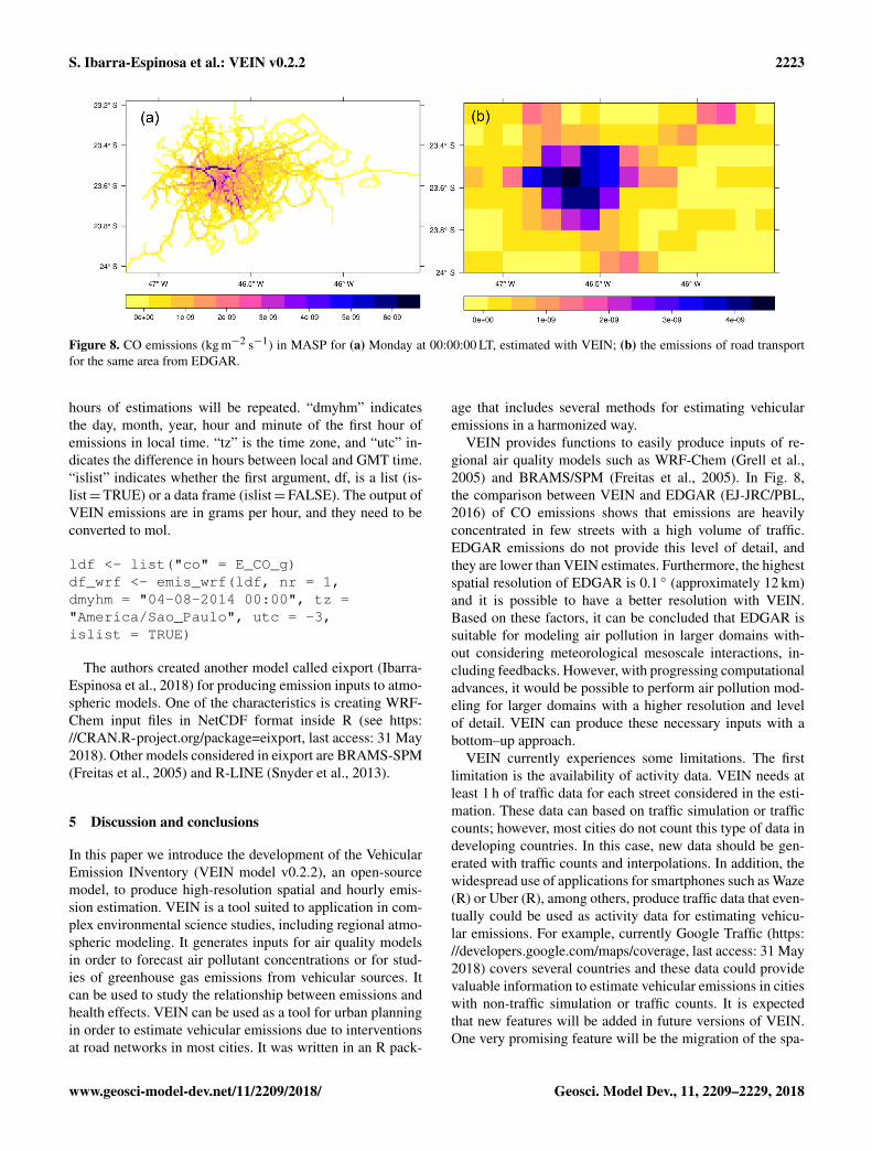
g <- make_grid(spobj = net, width =0.00976,height = 0.00976, polygon = T)E_CO_g <- emis_grid(spobj = net, g = g,sr = "+init=epsg:31983", type ="lines")

Figure 8a shows the resulting emissions of CO in a gridwith class SpatialPolygonsDataFrame built for agrid with a resolution of 1 km representing the base year2015. This emissions grid was built using the package sf(process shown in Appendix A). Figure 8b shows the COemissions grid of road transport from EDGAR for the same



area and base year 2010 (EJ-JRC/PBL, 2016), which is thelatest available year.

4.5 Speciation

Atmospheric simulations of ozone require knowledge aboutthe VOC compounds and particulate matter speciation,which are necessary for solving the different chemical mech-anisms. For example, a São Paulo study of ozone concentra-tions that used models BRAMS/SPM (Freitas et al., 2005)and WRF/Chem (Grell et al., 2005) involved detailed VOCspeciation (Andrade et al., 2015). It is important to mentionthat there is evidence to prove that reducing black carbonemissions would help lower the global radiative forcing andimprove population health (Bond et al., 2013). Hence, thespeciation of emissions is important and VEIN provides thisinformation. The VEIN function speciate splits VOC and PMinto their constituents. The arguments of these functions areemissions estimation, type of speciation, type of vehicle, fueland Euro standard. There are four types of PM speciation:“bcom” because it splits PM in black carbon and organicmatter (Ntziachristos and Samaras, 2016), “tire”, “brake” and“road” (Ntziachristos and Boulter, 2009). However, there iscurrently only one type of VOC speciation for MASP, the“iag” (Ibarra, 2017). The name of the speciation iag comesfrom the initials of the Institute of Astronomy, Geophysicsand Atmospheric Sciences of the University of São Paulo.The speciation iag is based on measurements made by stu-dents of this institute. The speciation iag splits the VOCemissions for the Carbon Bond Mechanism Z (CMB-Z; Za-veri and Peters, 1999). If the user intends to use other mecha-nisms, then the user needs to know how to speciate the VOCsand PM based on the user’s own data. This means that theuser must know the percentages needed to split the pollutantsand use them in the argument k of any VEIN function for theemission factor of the respective type of vehicle and then usethem to estimate the emissions of that fraction of vehicles.For example, if the user knows that 5 % of COV emissionsfor LDV consuming diesel are xylenes, then the user mustuse the function ef_ldv_speed or ef_ldv_scaled (or its ownlocal emission factors) with the argument k= 5/100. The ar-gument k is simply a factor added to the resulting emissionfunction. Finally, the user must aggregate the emissions bypollutant.

4.6 Input of atmospheric models

Meteorological factors influence the chemical process of pol-lutants in the atmosphere. Therefore, their transport and be-havior in the atmosphere must be predicted by a model thatincludes the meteorological components (“in-line” couplingof meteorology and chemistry), such as the Weather Re-search and Forecasting Chemistry model (WRF-Chem; Grellet al., 2005). This model has been widely used around theworld since its inception (2005 to 2006).

WRF-Chem requires gridded emission fluxes as inputdata. There are tools to assimilate top–down emissions in-ventories, such as EDGAR (Olivier et al., 1996) and REanal-ysis of the TROpospheric chemical composition (RETRO;Schultz, 2007), using the software PREP-Chem (Freitaset al., 2011). These tools are very important to the modelingcommunity; however, their spatial resolutions are very lim-ited. VEIN includes functions to generate WRF-Chem inputsfrom the emissions grid with any desired resolution in thefollowing way. VEIN estimates emissions of different pollu-tants at each street and also produces emissions grids neededto do the regional modeling. This is performed through thespatial intersection between emissions at streets and a poly-gon grid with the required resolution. The resulting grid hastotal emissions in each grid cell proportional to the length ofthe streets inside each cell.

Figure 8 shows a comparison for VEIN (Fig. 8a) andEDGAR (Fig. 8b), using an emissions inventory for the COin MASP. One may note that CO is spatially well representedfor VEIN by comparison with EDGAR. Furthermore, VEINoffers much more detail about the emission of this pollutant,which occurs mainly on urban motorways due to the highvolume of traffic on these roads. The total CO emissions us-ing VEIN are 1.73× 10−6 (kg m−2 s−1), considering the firstsecond of a typical Monday at 00:00 LT, and EDGAR givesemissions of 8.46× 10−8 (kg m−2 s−1). Therefore, VEIN es-timates are 20.50 times higher than EDGAR. This differencecould be higher if compared with the morning rush hour ofVEIN. However, it is important to mention that the estimatewith VEIN for this paper is illustrative, and that more de-tailed emissions inventories should be made when comparingit to others. For example, the inventory for this paper includesestimates only for LDVs assuming that all are PCs. It doesnot include other types of vehicles as the total amount of ve-hicles were not calibrated with fuel consumption. Ntziachris-tos and Samaras (2016) recommends comparing bottom–upestimates with fuel consumption in order to calibrate inputsof emissions inventory (traffic data in this case). These differ-ences highlight the need for development, intercomparisonand uncertainty evaluation of emission estimates. These re-sults are very useful for many scientific and standardizationpurposes such as health effects in air pollution studies, urbanplanning and strategies to cut greenhouse gas emissions.

The VEIN model provides functions to transform theemissions grids into inputs for the model Assimilating An-thropogenic Emissions (AS4WRF) (Vara-Vela et al., 2016).AAS4WRF consists of an NCL (Boulder, 2017) script thatreads the wrfinput file and an emissions text file producedby VEIN to create a WRF-Chem input file. The VEIN modelprovides the function emis_wrf to automatically create a dataframe in the correct format with the columns longitude, lati-tude, ID of grid cell, pollutants, local time and GMT time inthe format POSIXct. The arguments of emis_wrf are “sdf”,which is a list of SpatialPolygonsDataFrames; eachare given per pollutant. “nr” indicates how many times the



Figure 8. CO emissions (kg m−2 s−1) in MASP for (a) Monday at 00:00:00 LT, estimated with VEIN; (b) the emissions of road transportfor the same area from EDGAR.

hours of estimations will be repeated. “dmyhm” indicatesthe day, month, year, hour and minute of the first hour ofemissions in local time. “tz” is the time zone, and “utc” in-dicates the difference in hours between local and GMT time.“islist” indicates whether the first argument, df, is a list (is-list=TRUE) or a data frame (islist=FALSE). The output ofVEIN emissions are in grams per hour, and they need to beconverted to mol.

ldf <- list("co" = E_CO_g)df_wrf <- emis_wrf(ldf, nr = 1,dmyhm = "04-08-2014 00:00", tz ="America/Sao_Paulo", utc = -3,islist = TRUE)

The authors created another model called eixport (Ibarra-Espinosa et al., 2018) for producing emission inputs to atmo-spheric models. One of the characteristics is creating WRF-Chem input files in NetCDF format inside R (see https://CRAN.R-project.org/package=eixport, last access: 31 May2018). Other models considered in eixport are BRAMS-SPM(Freitas et al., 2005) and R-LINE (Snyder et al., 2013).

5 Discussion and conclusions

In this paper we introduce the development of the VehicularEmission INventory (VEIN model v0.2.2), an open-sourcemodel, to produce high-resolution spatial and hourly emis-sion estimation. VEIN is a tool suited to application in com-plex environmental science studies, including regional atmo-spheric modeling. It generates inputs for air quality modelsin order to forecast air pollutant concentrations or for stud-ies of greenhouse gas emissions from vehicular sources. Itcan be used to study the relationship between emissions andhealth effects. VEIN can be used as a tool for urban planningin order to estimate vehicular emissions due to interventionsat road networks in most cities. It was written in an R pack-

age that includes several methods for estimating vehicularemissions in a harmonized way.

VEIN provides functions to easily produce inputs of re-gional air quality models such as WRF-Chem (Grell et al.,2005) and BRAMS/SPM (Freitas et al., 2005). In Fig. 8,the comparison between VEIN and EDGAR (EJ-JRC/PBL,2016) of CO emissions shows that emissions are heavilyconcentrated in few streets with a high volume of traffic.EDGAR emissions do not provide this level of detail, andthey are lower than VEIN estimates. Furthermore, the highestspatial resolution of EDGAR is 0.1 ◦ (approximately 12 km)and it is possible to have a better resolution with VEIN.Based on these factors, it can be concluded that EDGAR issuitable for modeling air pollution in larger domains with-out considering meteorological mesoscale interactions, in-cluding feedbacks. However, with progressing computationaladvances, it would be possible to perform air pollution mod-eling for larger domains with a higher resolution and levelof detail. VEIN can produce these necessary inputs with abottom–up approach.

VEIN currently experiences some limitations. The firstlimitation is the availability of activity data. VEIN needs atleast 1 h of traffic data for each street considered in the esti-mation. These data can based on traffic simulation or trafficcounts; however, most cities do not count this type of data indeveloping countries. In this case, new data should be gen-erated with traffic counts and interpolations. In addition, thewidespread use of applications for smartphones such as Waze(R) or Uber (R), among others, produce traffic data that even-tually could be used as activity data for estimating vehicu-lar emissions. For example, currently Google Traffic (https://developers.google.com/maps/coverage, last access: 31 May2018) covers several countries and these data could providevaluable information to estimate vehicular emissions in citieswith non-traffic simulation or traffic counts. It is expectedthat new features will be added in future versions of VEIN.One very promising feature will be the migration of the spa-


https://CRAN.R-project.org/package=eixport

https://CRAN.R-project.org/package=eixport

https://developers.google.com/maps/coverage

https://developers.google.com/maps/coverage


tial dependencies into the new package, sf (spatial features)(Pebesma, 2016). This package provides S3 classes for han-dling spatial data faster than its predecessor, the package sp(Pebesma and Bivand, 2005).

The emission factors are another aspect of VEIN thatcan be enhanced in future versions. They could be sourcedfrom several emissions studies, such as tunnel studies (Pérez-Martinez et al., 2014; Martins et al., 2006), or others based ontraffic situations whereby emissions are sourced from driv-ing cycles (ARTEMIS for example, André, 2004) or otherexperimental campaigns (Corvalán and Vargas, 2003). TheInternational Vehicular Emissions (IVE) is a top–down ve-hicular emission model that has been used in different coun-tries to estimate vehicular emissions (González et al., 2017;Wang et al., 2008). It could be possible to derive emissionfactors from IVE and estimate their corresponding emissionsin VEIN, in order to use the capabilities of VEIN.

VEIN’s purpose is to serve as a tool for air quality researchand environmental management. Since air quality modelsneed detailed emissions species, VEIN was created with thefunction speciate. VEIN will add several new speciations tothese functions, such as those in the EMEP/EEA guidelines(Ntziachristos and Samaras, 2016). In the case of Brazil,there are several studies of tropospheric ozone, which usethe speciation of VOC emissions as input (Vara-Vela et al.,2016; Abou Rafee et al., 2017).

Code and data availability. VEIN is available at the Comprehen-sive R Archive Network (CRAN) https://CRAN.R-project.org/package=vein (last access: 31 May 2018) and github https://github.com/atmoschem/vein (last access: 31 May 2018); Changelogis available at https://github.com/atmoschem/vein/blob/master/NEWS.md (last access: 31 May 2018). The software version Ve-hicular Emissions INventories (VEIN) v0.2.2 was developed usingthe R programming language v3.4.1. For further information aboutthe VEIN package, contact the developer Sergio Ibarra-Espinosaat [email protected]. Datasets included emission factors fe2015and mileage functions fkm from the Environmental Agency of SãoPaulo (CETESB). In addition, emission and deterioration factorsare provided in the form of lookup tables from Copert (Ntziachris-tos and Samaras, 2016). These include hot emission factors forlight-duty vehicles (LDVs), heavy-duty vehicles (HDVs), cold start,evaporative factors, cold starts and resuspension and perform speci-ations. Emission factor functions are included for U.S. EPA/AP42(U.S. EPA, 2002) estimations with default parameters. There arealso two datasets to perform the example functions, a data frameto extrapolate morning peak hour vehicle traffic data to each hourof the week (pc_profile), and a vehicle start pattern (“pc_cold”)to be used for cold-start estimation. Moreover, VEIN includes atraffic simulation for the western region of São Paulo City named“net”. Software required: VEIN imports functions of the packagessp, sf, rgeos, rgdal, raster and units, which require libraries GDAL(>= 2.0.0), GEOS (>= 3.4.0) and UDUNITS-2.




https://github.com/atmoschem/vein

https://github.com/atmoschem/vein

https://github.com/atmoschem/vein/blob/master/NEWS.md

https://github.com/atmoschem/vein/blob/master/NEWS.md


Appendix A: Intercept grid and street emissions

Development versions of VEIN already include support forsf including the procedure shown in this Appendix.

library(vein)library(sf)# Converting objects into "sf" andprojecting to UTM zone 23S - EPSG:31983g_sf <- st_as_sf(spTransform(g,CRSobj = "+init=epsg:31983"))net_sf <- st_as_sf(spTransform(net,CRSobj = "+init=epsg:31983"))# Calculating initial length of net_sfnet_sf$LKM <- st_length(st_cast(net_sf[st_dimension(net_sf) == 1,]))# Intersecting net and gridnet_sf_g <- st_intersection(net_sf, g_sf)

# Calculating new length of net_sfnet_sf_g$LKM2 <- st_length(st_cast(net_sf_g[st_dimension(net_sf_g) ==1,]))# Checking dimensionsdim(net_sf_g)# Converting from sf to data.framenet_sf_gg <- as.data.frame(net_sf_g)# Eliminating column ’geometry’net_sf_gg <- net_sf_gg[,-171]# Obtaining proportional emissionsof 168 hours of the weeknet_sf_gg[,1:168] <- net_sf_gg[,1:168] *

as.numeric(net_sf_gg$LKM2/net_sf_gg$LKM)# Agregating emissions by id of griddfm <- aggregate(cbind(net_sf_gg[, 1:168]),

by = list(net_sf_gg$id),

sum, na.rm = TRUE)# naming columns of data-frame dfmnames(dfm) <- c("id", paste0("h", 1:168))

# Creating data-frame for id of gridgx <- data.frame(id = g$id)# merging data-framesgx <- merge(gx, dfm, by="id", all.x = T)# Generating spatial grid andconverting to "Spatial"E_CO_g <- as(st_sf(gx,geometry = g_sf$geometry), "Spatial")# Converting to WGS84 lat lonE_CO_g <- spTransform(E_CO_g,"+init=epsg:4326")

Appendix B: Examples using VEIN with differentemission factors

B1 Activity data

data(net)data(pc_profile)data(fe2015)pc1 <- age_ldv(x = net$ldv, name = "PC")pcw <- temp_fact(net$ldv+net$hdv, pc_profile)

speed <- netspeed(pcw, net$ps, net$ffs,net$capacity, net$lkm, alpha = 1)

B2 Emission factors

B2.1 Copert emission factors (without correction ofdeterioration and fuel effects)

euro <- c(rep("V", 5), rep("IV", 5),rep("III", 5), rep("II", 5),

rep("I", 5), rep("PRE", 15))lef1 <- lapply(1:40, function(i) {ef_ldv_speed(v = "PC", t = "4S",cc = "<=1400", f = "G",

eu = euro[i], p = "CO",show.equation = FALSE) })

B2.2 Local emission factors of passenger cars usinggasoline, constant by age of use

co1 <- fe2015[fe2015$Pollutant=="CO", ]lef2 <- EmissionFactorsList(co1$PC_G)

B2.3 Scaled emission factors

lef3 <- ef_ldv_scaled(dfcol = co1$PC_G,v = "PC", t = "4S", cc = "<=1400",f = "G",p = "CO", eu=co1$Euro_LDV)

B3 Estimations

E_COv1 <- emis(veh = pc1,lkm = net$lkm,ef = lef1, speed = speed,

profile = pc_profile)E_COv2 <- emis(veh = pc1,lkm = net$lkm,ef = lef2, speed = speed,

profile = pc_profile)E_COv3 <- emis(veh = pc1,lkm = net$lkm,ef = lef3, speed = speed,

profile = pc_profile)



Author contributions. SIE designed and implemented the entiremodel. All authors contributed to the final manuscript.

Competing interests. The authors declare they have no actual or po-tential competing interest.

Acknowledgements. We thank the Environmental Agency ofSão Paulo State (CETESB), the programs CAPES and CNPQ(Ministry of Education, Brazil), and CONICYT (Ministry ofEducation, Chile). This work was also partially supported by theFONDAP/CONICYT 15110009 project. These entities provideddata and support that were invaluable to this study. We also thankProf. Dr. Zissis Samaras and Prof. Dr. Leonidas Ntziachristos fromAristotle University, since VEIN relies heavily on all their researchabout vehicular emissions and the model Copert.

Edited by: Augustin ColetteReviewed by: two anonymous referees

References

Abou Rafee, S. A., Martins, L. D., Kawashima, A. B., Almeida,D. S., Morais, M. V. B., Souza, R. V. A., Oliveira, M. B. L.,Souza, R. A. F., Medeiros, A. S. S., Urbina, V., Freitas, E. D.,Martin, S. T., and Martins, J. A.: Contributions of mobile, sta-tionary and biogenic sources to air pollution in the Amazonrainforest: a numerical study with the WRF-Chem model, At-mos. Chem. Phys., 17, 7977–7995, https://doi.org/10.5194/acp-17-7977-2017, 2017.

Albuquerque, T.: Distribuição de tamanho, composição química eidentificação das fontes de aerossol atmosférico de São Paulo:Um estudo de caso para o inverno de 2003, Ph.D. thesis, SãoPaulo: University of São Paulo, 2005.

Andrade, M. D. F., Ynoue, R. Y., Freitas, E. D., Tode-sco, E., Vara Vela, A., Ibarra, S., Martins, L. D., Martins,J. A., and Carvalho, V. S. B.: Air quality forecasting sys-tem for Southeastern Brazil, Front. Environ. Sci., 3, 1–12,https://doi.org/10.3389/fenvs.2015.00009, 2015.

Andrade, M. D. F., Kumar, P., de Freitas, E. D., Ynoue,R. Y., Martins, J., Martins, L. D., Nogueira, T., Perez-Martinez, P., de Miranda, R. M., Albuquerque, T., Gonçalves,F. L. T., Oyama, B., and Zhang, Y.: Air quality inthe megacity of São Paulo: Evolution over the last 30years and future perspectives, Atmos. Environ., 159, 66–82,https://doi.org/10.1016/j.atmosenv.2017.03.051, 2017.

André, M.: The ARTEMIS European driving cycles for measuringcar pollutant emissions, Sci. Total. Environ., 334, 73–84, 2004.

ARTESP: Toll station count data, available at: http://www.artesp.sp.gov.br/ (last access: 31 May 2018), 2012.

Barlow, T., Latham, S., McCrae, I., and Boulter, P.: A referencebook of driving cycles for use in the measurement of road vehicleemissions, TRL Published Project Report, 2009.

Bivand, R. and Lewin-Koh, N.: maptools: Tools for Reading andHandling Spatial Objects, available at: http://CRAN.R-project.org/package=maptools (last access: 31 May 2018), r packageversion 0.8-34, 2015.

Bivand, R. and Rundel, C.: rgeos: Interface to Geometry Engine– Open Source (GEOS), available at: https://CRAN.R-project.org/package=rgeos (last access: 31 May 2018), r package version0.3-21, 2016.

Bivand, R., Pebesma, E., and Gomez-Rubio, V.: Applied spatialdata analysis with R, Springer, NY, available at: http://www.asdar-book.org/ (last access: 31 May 2018), 2013.

Bivand, R., Keitt, T., and Rowlingson, B.: rgdal: Bindings for theGeospatial Data Abstraction Library, available at: https://CRAN.R-project.org/package=rgdal (last access: 31 May 2018), r pack-age version 1.1-10, 2016.

Bond, T. C., Doherty, S. J., Fahey, D. W., Forster, P. M., Berntsen,T., DeAngelo, B. J., Flanner, M. G., Ghan, S., Kärcher, B.,Koch, D., Kinne, S., Kondo, Y., Quinn, P. K., Sarofim, M. C.,Schultz, M. G., Schulz, M., Venkataraman, C., Zhang, H., Zhang,S., Bellouin, N., Guttikunda, S. K., Hopke, P. K., Jacobson,M. Z., Kaiser, J. W., Klimont, Z., Lohmann, U., Schwarz, J. P.,Shindell, D., Storelvmo, T., Warren, S. G., and Zender, C. S.:Bounding the role of black carbon in the climate system: A sci-entific assessment, J. Geophys. Res.-Atmos., 118, 5380–5552,https://doi.org/10.1002/jgrd.50171, 2013.

Boulder, C. U.: The NCAR Command Language (NCL) (version6.4. 0), https://doi.org/10.5065/D6WD3XH5, 2017.

Boulter, P.: Environmental traffic management: A review of fac-tors affecting cold start emissions, Tech. rep., Transport Re-search Laboratory, Old Wokingham Road, Crowthorne, Berk-shire, RG45 6AU, UK, 1997.

Bruni, A. D. C. and Bales, M. P.: Curvas de intensidade deuso por tipo de veículo automotor da frota da cidadede São Paulo, Tech. rep., CETESB, available at: http://cetesb.sp.gov.br/veicular/wp-content/uploads/sites/6/2013/12/curvas-intensidade-uso-veiculos-automotores-cidade-sao-paulo.pdf (last access: 31 May 2018), 2013.

Bureau of Public Roads: Traffic and assignment mannual, Tech.rep., Dept. of Commerce, Urban Planning Division, WashingtonD.C., 1964.

Carslaw, D. C. and Ropkins, K.: Openair – an R package for airquality data analysis, Environ. Modell. Softw., 27, 52–61, 2012.

CET: Simulação de tráfego para Região Metropolitana de SãoPaulo, available at: http://www.cetsp.com.br (last access: 31 May2018), 2014.

CETESB: Emissões Veiculares no Estado de São Paulo, availableat: http://veicular.cetesb.sp.gov.br/relatorios-e-publicacoes/ (lastaccess: 31 May 2018), 2013.

CETESB: Emissões Veiculares no Estado de São Paulo, availableat: http://veicular.cetesb.sp.gov.br/relatorios-e-publicacoes/ (lastaccess: 31 May 2018), 2016.

Chen, R.-H., Chiang, L.-B., Chen, C.-N., and Lin, T.-H.: Cold-startemissions of an SI engine using ethanol–gasoline blended fuel,Appl. Therm. Eng., 31, 1463–1467, 2011.

CONAMA: Programa de controle de emissões veiculares (Pro-conve), available at: http://www.mma.gov.br/port/conama/res/res86/res1886.html (last access: 21 January 2014), 1986.

Corvalán, R. M. and Vargas, D.: Experimental analysis of emissiondeterioration factors for light duty catalytic vehicles Case study:Santiago, Chile, Trans. Res. D, 8, 315–322, 2003.

Corvalán, R. M., Osses, M., and Urrutia, C. M.: Hot emission modelfor mobile sources: application to the metropolitan region of the


https://doi.org/10.5194/acp-17-7977-2017

https://doi.org/10.5194/acp-17-7977-2017

https://doi.org/10.3389/fenvs.2015.00009

https://doi.org/10.1016/j.atmosenv.2017.03.051

http://www.artesp.sp.gov.br/

http://www.artesp.sp.gov.br/

http://CRAN.R-project.org/package=maptools

http://CRAN.R-project.org/package=maptools

https://CRAN.R-project.org/package=rgeos

https://CRAN.R-project.org/package=rgeos

http://www.asdar-book.org/

http://www.asdar-book.org/

https://CRAN.R-project.org/package=rgdal

https://CRAN.R-project.org/package=rgdal

https://doi.org/10.1002/jgrd.50171

https://doi.org/10.5065/D6WD3XH5

http://cetesb.sp.gov.br/veicular/wp-content/uploads/sites/6/2013/12/curvas-intensidade-uso-veiculos-automotores-cidade-sao-paulo.pdf




http://www.cetsp.com.br

http://veicular.cetesb.sp.gov.br/relatorios-e-publicacoes/

http://veicular.cetesb.sp.gov.br/relatorios-e-publicacoes/

http://www.mma.gov.br/port/conama/res/res86/res1886.html

http://www.mma.gov.br/port/conama/res/res86/res1886.html


city of Santiago, Chile, J. Air Waste Manage. Assoc., 52, 167–174, 2002.

Davis, N., Lents, J., Osses, M., Nikkila, N., and Barth, M.: Part3: Developing countries: development and application of an in-ternational vehicle emissions model, Transportation ResearchRecord, J. Trans. Res. Board, 8, 155–165, 2005.

DENATRAN: National Department of Traffic Road, availableat: chttp://www.denatran.gov.br/frota2015.htm (last access: 4February 2016), 2015.

Directive70/220/EEC: Measures to be taken against the emis-sion of gaseous pollutants from diesel engines for use in ve-hicles, available at: http://eur-lex.europa.eu/legal-content/EN/TXT/PDF/?uri=CELEX:31991L0441&from=EN (last access:31 May 2018), 1991.

EEA: Emission Inventory Report 1990–2011 Under the UNECEConvention on LRTAP, European Environment Agency, Luxem-bourg, 2013.

EJ-JRC/PBL: Emission Database for Global Atmospheric Research(EDGAR), release EDGAR v4.3.1_v2 (1970–2010), available at:http://edgar.jrc.ec.europa.eu (last access: 31 May 2018), 2016.

U.S. EPA: Comprehensive analysis of biodiesel impacts on exhaustemissions, Tech. rep., Draft Technical Report, EPA420-02-001,2002.

Freitas, E., Martins, L., Silva Dias, P., and Andrade, M. D. F.: Asimple photochemical module implemented in RAMS for tropo-spheric ozone concentration forecast in the metropolitan area ofSão Paulo, Brazil: Coupling and validation, Atmos. Environ., 39,6352–6361, 2005.

Freitas, S. R., Longo, K. M., Alonso, M. F., Pirre, M., Mare-cal, V., Grell, G., Stockler, R., Mello, R. F., and SánchezGácita, M.: PREP-CHEM-SRC – 1.0: a preprocessor of tracegas and aerosol emission fields for regional and global atmo-spheric chemistry models, Geosci. Model Dev., 4, 419–433,https://doi.org/10.5194/gmd-4-419-2011, 2011.

González, C., Gómez, C., Rojas, N., Acevedo, H., and Aristizábal,B.: Relative impact of on-road vehicular and point-source indus-trial emissions of air pollutants in a medium-sized Andean city,Atmos. Environ., 152, 279–289, 2017.

Grell, G. A., Peckham, S. E., Schmitz, R., McKeen, S. A., Frost, G.,Skamarock, W. C., and Eder, B.: Fully coupled “online” chem-istry within the WRF model, Atmos. Environ., 39, 6957–6975,2005.

Hijmans, R. J.: raster: Geographic Data Analysis and Modeling,available at: https://CRAN.R-project.org/package=raster (lastaccess: 31 May 2018), r package version 2.5-8, 2016.

Ibarra, S.: Air pollution modeling in São Paulo using bottom-upvehicular emissions inventories, Ph.D. thesis, São Paulo: Univer-sity of São Paulo, available at: http://www.iag.usp.br/pos/sites/default/files/t_sergio_a_i_espinosa_corrigida.pdf (last access: 31May 2018), 2017.

Ibarra-Espinosa, S.: vein: Vehicular Emissions Inventories, R pack-age version 0.2.2-25, available at: https://CRAN.R-project.org/package=veinhttps://github.com/atmoschem/vein (last access: 31May 2018), 2017.

Ibarra-Espinosa, S. and Pebesma, E.: ibarraespinosa/vein: VEINv0.2.2 (Version v0.2.2), Zenodo, available at: https://doi.org/10.5281/zenodo.1039236 (last access: 31 May 2018), 2017.

Ibarra-Espinosa, S. and Ynoue, R.: REMI model: Bottom-up emis-sions inventories for cities with lack of data, J. Earth Sci.Geotech. Eng., 1, 277–288, 2017.

Ibarra-Espinosa, S., Schuch, D., and Dias de Freitas, E.: eixport:An R package to export emissions to atmospheric models, J.Open Source Softw., 3, 607, https://doi.org/10.21105/joss.00607,2018.

IBGE: Instituto Brasileiro de Geografia e Estatística – Población es-timada 2014, available at: http://cod.ibge.gov.br/232IH, last ac-cess: 12 December, 2014.

Kahle, D. and Wickham, H.: ggmap: Spatial Visualization withggplot2, The R J., 5, 144–161, available at: http://journal.r-project.org/archive/2013-1/kahle-wickham.pdf (last access: 31May 2018), 2013.

Koupal, J., Cumberworth, M., Michaels, H., Beardsley, M., andBrzezinski, D.: Design and Implementation of MOVES: EPA’sNew Generation Mobile Source Emission Model, Ann Arbor,1001, 48 105, 2003.

Kucharski, R. and Drabicki, A.: Estimating Macroscopic Vol-ume Delay Functions with the Traffic Density Derived fromMeasured Speeds and Flows, J. Adv. Transp., 2017, 4629792,https://doi.org/10.1155/2017/4629792, 2017.

Lam, W. H. and Xu, J.: Estimation of AADT from short periodcounts in Hong Kong – A comparison between neural networkmethod and regression analysis, J. Adv. Transp., 34, 249–268,2000.

Leiner, B. M., Cerf, V. G., Clark, D. D., Kahn, R. E., Kleinrock, L.,Lynch, D. C., Postel, J., Roberts, L. G., and Wolff, S. S.: The pastand future history of the Internet, Commun. ACM, 40, 102–108,1997.

Lents, J., Davis, N., Nikkila, N., and Osses, M.: São Paulo Vehi-cle Activity Study, Tech. rep., International Sustainable SystemResearch Center, 605 South Palm Street, Suite C, La Habra, CA90631, USA, 2004.

Ludykar, D., Westerholm, R., and Almen, J.: Cold start emissions at+22, -7 and -20 C ambient temperatures from a three-way cata-lyst (TWC) car: regulated and unregulated exhaust components,Sci. Total Environ., 235, 65–69, 1999.

Manual, H. C.: Highway capacity manual, Washington, DC, p. 11,2000.

Manzo, S., Nielsen, O., and Prato, C.: Effects of Uncertainty inSpeed-Flow Curve Parameters on a Large-Scale Model: CaseStudy of the Danish National Model, Transportation ResearchRecord: J. Transport. Res. Board, 2429, ,30–37, 2014.

Martins, L. D., Andrade, M. F., Freitas, E. D., Pretto, A., Gatti, L. V.,Albuquerque, É. L., Tomaz, E., Guardani, M. L., Martins, M. H.,and Junior, O. M.: Emission factors for gas-powered vehiclestraveling through road tunnels in São Paulo, Brazil, Environ. Sci.Technol., 40, 6722–6729, https://doi.org/10.1021/es052441u,2006.

Mellios, G. and Ntziachristos, L.: EMEP/EEA emission inventoryguidebook; Gasoline evaporation from vehicles, Tech. rep., Eu-ropean Environment Agency, Copenhagen, 2016.

Ministério do Meio Ambiente: Primeiro Inventário Nacionalde Emissões Atmosféricas por Veículos AutomotoresRodoviários, available at: http://www.mma.gov.br/estruturas/163/_publicacao/163_publicacao27072011055200.pdf (lastaccess: 31 May 2018), 2011.


chttp://www.denatran.gov.br/frota2015.htm

http://eur-lex.europa.eu/legal-content/EN/TXT/PDF/?uri=CELEX:31991L0441&from=EN

http://eur-lex.europa.eu/legal-content/EN/TXT/PDF/?uri=CELEX:31991L0441&from=EN

http://edgar.jrc.ec.europa.eu

https://doi.org/10.5194/gmd-4-419-2011

https://CRAN.R-project.org/package=raster

http://www.iag.usp.br/pos/sites/default/files/t_sergio_a_i_espinosa_corrigida.pdf

http://www.iag.usp.br/pos/sites/default/files/t_sergio_a_i_espinosa_corrigida.pdf

https://CRAN.R-project.org/package=vein https://github.com/atmoschem/vein

https://CRAN.R-project.org/package=vein https://github.com/atmoschem/vein

https://doi.org/10.5281/zenodo.1039236

https://doi.org/10.5281/zenodo.1039236

https://doi.org/10.21105/joss.00607

http://cod.ibge.gov.br/232IH

http://journal.r-project.org/archive/2013-1/kahle-wickham.pdf

http://journal.r-project.org/archive/2013-1/kahle-wickham.pdf

https://doi.org/10.1155/2017/4629792

https://doi.org/10.1021/es052441u

http://www.mma.gov.br/estruturas/163/_publicacao/163_publicacao27072011055200.pdf

http://www.mma.gov.br/estruturas/163/_publicacao/163_publicacao27072011055200.pdf


Miranda, R.: Caracterização físico química e propriedades ópticasde aerossol urbano da região metropolitana de São Paulo, Ph.D.thesis, São Paulo: University of São Paulo, 2001.

MMA: Air Pollution Control Program by Motor Vehicles; PRO-CONVE/PROMOT, available at: http://www.ibama.gov.br/phocadownload/category/4?download=4793%3Amanual-ingles(last access: 8 September 2015), 2011.

MMA: PROCONVE: PROGRAMA DE CONTROLE DEPOLUIÇÃO DO AR POR VEÃ CULOS AUTOMOTORES,available at: http://www.mma.gov.br/estruturas/163/_arquivos/proconve_163.pdf, last access: 8 September, 2015.

Nogueira, T., de Souza, K. F., Fornaro, A., de Fatima Andrade,M., and de Carvalho, L. R. F.: On-road emissions of carbonylsfrom vehicles powered by biofuel blends in traffic tunnels in theMetropolitan Area of Sao Paulo, Brazil, Atmos. Environ., 108,88–97, 2015.

Ntziachristos, L. and Boulter, P.: EMEP/EEA emission inventoryguidebook; Road Transport: Automobile tyre and break wearand road abrasion, European Environment Agency, Copenhagen,2009.

Ntziachristos, L. and Samaras, Z.: EMEP/EEA emission inventoryguidebook; Road Transport: Passenger cars, Light commercialtrucks, Heavy-duty vehicles including buses and Motorcycles,European Environment Agency, Copenhagen, 2016.

Oliveira, M.: Evolução das distribuições de tamanho em massa enúmero do aerossol atmosférico em São Paulo, Ph.D. thesis, SãoPaulo: University of São Paulo, 2007.

Olivier, J. G. J., Bouwman, A. F., van der Maas, C. W. M.,Berdowski, J. J. M., Veldt, C., Bloos, J. P. J., Visschedijk, A.J. H., Zandveld, P. Y. J., and Haverlag, J. L.: Description ofEDGAR Version 2.0: A set of global emission inventories ofgreenhouse gases and ozone-depleting substances for all anthro-pogenic and most natural sources on a per country basis and on1 degree × 1 degree grid, National Institute of Public Health andthe Environment (Rijksinstituut voor Volksgezondheid en MilieuRIVM), No. RIVM report: 771060 002, 1996.

Paustian, K., Ravindranath, N., and van Amstel, A.: IPCC Guide-lines for National Greenhouse Gas Inventories, Tech. rep., 2006.

Pebesma, E.: sf: Simple Features for R, available at: https://github.com/edzer/sfr/ (last access: 31 May 2018), r package version 0.4-3, 2016.

Pebesma, E. and Bivand, R.: Classes and methods for spatial data inR, available at: http://cran.r-project.org/doc/Rnews/ (last access:31 May 2018), 2005.

Pebesma, E., Mailund, T., and Hiebert, J.: Measurement Units in R,The R J., 8, 486–494, available at: https://journal.r-project.org/archive/2016-2/pebesma-mailund-hiebert.pdf (last access: 31May 2018), 2016.

Pérez-Martinez, P., Miranda, R., Nogueira, T., Guardani, M.,Fornaro, A., Ynoue, R., and Andrade, M.: Emission factors ofair pollutants from vehicles measured inside road tunnels in SãoPaulo: case study comparison, Int. J. Environ. Sci. Technol., 11,2155–2168, 2014.

Perugu, H., Wei, H., and Yao, Z.: Developing high-resolution ur-ban scale heavy-duty truck emission inventory using the data-driven truck activity model output, Atmos. Environ., 155, 210–230, 2017.

Pulles, T. and Heslinga, D.: The art of emission inventorying, TNO,Utrecht, 2010.

R Core Team: R: A Language and Environment for Statistical Com-puting, R Foundation for Statistical Computing, Vienna, Aus-tria, available at: http://www.R-project.org/ (last access: 31 May2018), 2017.

Rafee, S.: Estudo numerico do impacto das emissoes veiculares efixas da cidade de Manaus nas concentracoes de poluentes at-mosfericos da regiao amazonica, Master’s thesis, Londrina: Uni-versidade Tecnologica Federal do Parana, 2015.

Schultz, M. G.: REanalysis of the TROpospheric chemical compo-sition over the past 40 years, Max-Planck Institute for Meteorol-ogy, 48, ISSN: 1614-1199, Series: Earth System Science, Ham-burg, Germany, 2007.

Seinfeld, J. H. and Pandis, S. N.: Atmospheric chemistry andphysics: from air pollution to climate change, 3rd Edn., John Wi-ley & Sons, New Jersey, US, ISBN: 978118947401 2016.

Smit, R., Ntziachristos, L., and Boulter, P.: Validation of road ve-hicle and traffic emission models – A review and meta-analysis,Atmos. Environ., 44, 2943–2953, 2010.

Snyder, M. G., Venkatram, A., Heist, D. K., Perry, S. G., Petersen,W. B., and Isakov, V.: RLINE: A line source dispersion modelfor near-surface releases, Atmos. Environ., 77, 748–756, 2013.

Streets, D. G., Bond, T., Carmichael, G., Fernandes, S., Fu, Q., He,D., Klimont, Z., Nelson, S., Tsai, N., Wang, M. Q., Woo, J. H.,and Yarber, K. F.: An inventory of gaseous and primary aerosolemissions in Asia in the year 2000, J. Geophys. Res.-Atmos.,108, D21, https://doi.org/10.1029/2002JD003093, 2003.

Suh, S., Park, C.-H., and Kim, T. J.: A highway capacity functionin Korea: measurement and calibration, Transport. Res. A, 24,177–186, 1990.

U.S. EPA: National Emissions Inventory (NEI), avail-able at: https://www.epa.gov/air-emissions-inventories/national-emissions-inventory-nei, last access: 31 May 2018.

U.S. EPA: AP42 Compilation of emission factors; Resuspenssionemissions from paved roads, Environment Protection Agency,USA, 2016.

Vara-Vela, A., Andrade, M. F., Kumar, P., Ynoue, R. Y., and Muñoz,A. G.: Impact of vehicular emissions on the formation of fineparticles in the São Paulo Metropolitan Area: a numerical studywith the WRF-Chem model, Atmos. Chem. Phys., 16, 777–797,https://doi.org/10.5194/acp-16-777-2016, 2016.

Wang, H., Chen, C., Huang, C., and Fu, L.: On-road vehicle emis-sion inventory and its uncertainty analysis for Shanghai, China,Sci. Total Environ., 398, 60–67, 2008.

Wang, X. and Kockelman, K.: Forecasting network data: Spatial in-terpolation of traffic counts from texas data, Trans. Res. Record:J. Transp. Res. Board, 1, 100–108, 2009.

Weilenmann, M., Favez, J.-Y., and Alvarez, R.: Cold-startemissions of modern passenger cars at different lowambient temperatures and their evolution over vehiclelegislation categories, Atmos. Environ., 43, 2419–2429,https://doi.org/10.1016/j.atmosenv.2009.02.005, 2009.

Wickham, H.: ggplot2: elegant graphics for data analysis, SpringerNew York, available at: https://www.springer.com/us/book/9780387981413 (last access: 31 May 2018), 2009.

Ynoue, R.: Modelagem numérica da formação, crescimento e trans-porte das partículas inorgânicas secundárias constituintes doaerossol urbano na região metropolitana de São Paulo, Ph.D. the-sis, São Paulo: University of São Paulo, 2004.


http://www.ibama.gov.br/phocadownload/category/4?download=4793%3Amanual-ingles

http://www.ibama.gov.br/phocadownload/category/4?download=4793%3Amanual-ingles

http://www.mma.gov.br/estruturas/163/_arquivos/proconve_163.pdf

http://www.mma.gov.br/estruturas/163/_arquivos/proconve_163.pdf

https://github.com/edzer/sfr/

https://github.com/edzer/sfr/

http://cran.r-project.org/doc/Rnews/

https://journal.r-project.org/archive/2016-2/pebesma-mailund-hiebert.pdf

https://journal.r-project.org/archive/2016-2/pebesma-mailund-hiebert.pdf

http://www.R-project.org/

https://doi.org/10.1029/2002JD003093

https://www.epa.gov/air-emissions-inventories/national-emissions-inventory-nei

https://www.epa.gov/air-emissions-inventories/national-emissions-inventory-nei

https://doi.org/10.5194/acp-16-777-2016

https://doi.org/10.1016/j.atmosenv.2009.02.005

https://www.springer.com/us/book/9780387981413

https://www.springer.com/us/book/9780387981413


Zaveri, R. A. and Peters, L. K.: A new lumped structure photochem-ical mechanism for large-scale applications, J. Geophys. Res.-Atmos., 104, 30387–30415, 1999.


VEIN v0.2.2: an R package for bottom–up vehicular ... · 2Department of Pathology, Faculdade de...

Documents

Transcript of VEIN v0.2.2: an R package for bottom–up vehicular ... · 2Department of Pathology, Faculdade de...