Vector elds and di erential forms - Department of...

Vector fields and differential forms

William G. Faris

April 28, 2006

Contents

I Analysis on a manifold 1

1 Vectors 31.1 Linear algebra . . . . . . . . . . . . . . . . . . . . . . . . . . . . . 31.2 Manifolds . . . . . . . . . . . . . . . . . . . . . . . . . . . . . . . 31.3 Local and global . . . . . . . . . . . . . . . . . . . . . . . . . . . 41.4 A gas system . . . . . . . . . . . . . . . . . . . . . . . . . . . . . 41.5 Vector fields . . . . . . . . . . . . . . . . . . . . . . . . . . . . . . 51.6 Systems of ordinary differential equations . . . . . . . . . . . . . 61.7 The straightening out theorem . . . . . . . . . . . . . . . . . . . 71.8 Linearization at a zero . . . . . . . . . . . . . . . . . . . . . . . . 81.9 Problems . . . . . . . . . . . . . . . . . . . . . . . . . . . . . . . 10

2 Forms 112.1 The dual space . . . . . . . . . . . . . . . . . . . . . . . . . . . . 112.2 Differential 1-forms . . . . . . . . . . . . . . . . . . . . . . . . . . 122.3 Ordinary differential equations in two dimensions . . . . . . . . . 142.4 The Hessian matrix and the second derivative test . . . . . . . . 152.5 Lagrange multipliers . . . . . . . . . . . . . . . . . . . . . . . . . 172.6 Covariant and contravariant . . . . . . . . . . . . . . . . . . . . . 182.7 Problems . . . . . . . . . . . . . . . . . . . . . . . . . . . . . . . 20

3 The exterior derivative 213.1 The exterior product . . . . . . . . . . . . . . . . . . . . . . . . . 213.2 Differential r-forms . . . . . . . . . . . . . . . . . . . . . . . . . . 223.3 Properties of the exterior derivative . . . . . . . . . . . . . . . . 233.4 The integrability condition . . . . . . . . . . . . . . . . . . . . . . 243.5 Gradient, curl, divergence . . . . . . . . . . . . . . . . . . . . . . 253.6 Problems . . . . . . . . . . . . . . . . . . . . . . . . . . . . . . . 26

4 Integration and Stokes’s theorem 274.1 One-dimensional integrals . . . . . . . . . . . . . . . . . . . . . . 274.2 Integration on manifolds . . . . . . . . . . . . . . . . . . . . . . . 284.3 The fundamental theorem . . . . . . . . . . . . . . . . . . . . . . 294.4 Green’s theorem . . . . . . . . . . . . . . . . . . . . . . . . . . . 29

iii

iv CONTENTS

4.5 Stokes’s theorem . . . . . . . . . . . . . . . . . . . . . . . . . . . 304.6 Gauss’s theorem . . . . . . . . . . . . . . . . . . . . . . . . . . . 314.7 The generalized Stokes’s theorem . . . . . . . . . . . . . . . . . . 314.8 References . . . . . . . . . . . . . . . . . . . . . . . . . . . . . . . 314.9 Problems . . . . . . . . . . . . . . . . . . . . . . . . . . . . . . . 33

II Analysis with a volume 35

5 The divergence theorem 375.1 Contraction . . . . . . . . . . . . . . . . . . . . . . . . . . . . . . 375.2 Duality . . . . . . . . . . . . . . . . . . . . . . . . . . . . . . . . 385.3 The divergence theorem . . . . . . . . . . . . . . . . . . . . . . . 395.4 Integration by parts . . . . . . . . . . . . . . . . . . . . . . . . . 405.5 A variant on curl . . . . . . . . . . . . . . . . . . . . . . . . . . . 405.6 Problems . . . . . . . . . . . . . . . . . . . . . . . . . . . . . . . 42

III Analysis with a Riemannian metric 43

6 The metric 456.1 Inner product . . . . . . . . . . . . . . . . . . . . . . . . . . . . . 456.2 Riemannian metric . . . . . . . . . . . . . . . . . . . . . . . . . . 466.3 Gradient and divergence . . . . . . . . . . . . . . . . . . . . . . . 476.4 Gradient dynamics . . . . . . . . . . . . . . . . . . . . . . . . . . 486.5 The Laplace operator . . . . . . . . . . . . . . . . . . . . . . . . 486.6 Curl . . . . . . . . . . . . . . . . . . . . . . . . . . . . . . . . . . 496.7 Problems . . . . . . . . . . . . . . . . . . . . . . . . . . . . . . . 50

7 Applications 517.1 Conservation laws . . . . . . . . . . . . . . . . . . . . . . . . . . 517.2 Maxwell’s equations . . . . . . . . . . . . . . . . . . . . . . . . . 527.3 Problems . . . . . . . . . . . . . . . . . . . . . . . . . . . . . . . 56

8 Length and area 578.1 Length . . . . . . . . . . . . . . . . . . . . . . . . . . . . . . . . . 578.2 Area . . . . . . . . . . . . . . . . . . . . . . . . . . . . . . . . . . 58

Part I

Analysis on a manifold

1

Chapter 1

Vectors

1.1 Linear algebra

The algebraic setting is an n-dimensional real vector space V with real scalars.However we shall usually emphasize the cases n = 2 (where it is easy to drawpictures) and n = 3 (where it is possible to draw pictures).

If u and v are vectors in V , and if a, b are real scalars, then the linearcombination au + vv is also a vector in V . In general, linear combinations areformed via scalar multiplication and vector addition. Each vector in this spaceis represented as an arrow from the origin to some point in the plane. A scalarmultiple cu of a vector u scales it and possibly reverses its direction. The sumu + v of two vectors u,v is defined by the parallelogram law Figure ??. Theoriginal two arrows determine a parallelogram, and the sum arrow runs fromthe origin to the opposite corner of the parallelogram.

1.2 Manifolds

An n-dimensional manifold is a set whose points are characterized by the valuesof n coordinate functions. Mostly we shall deal with examples when n is 1, 2,or 3.

We say that an open subset U of Rn is a nice region if it is diffeomorphicto an open ball in Rn. Each such nice region U is diffeomorphic to each othernice region V . For the moment the only kind of manifold that we consider isa manifold described by coordinates that put the manifold in correspondencewith a nice region. Such a manifold can be part of a larger manifold, as we shallsee later.

Thus this preliminary concept of manifold is given by a set M such thatthere are coordinates x1, . . . , xn that map M one-to-one onto some nice regionU in Rn. There are many other coordinate systems u1, . . . , un defined on M .What is required is that they are all related by diffeomorphisms, that is, if onegoes from U to M to V by taking the coordinate values of x1, . . . , xn back to the

3

4 CHAPTER 1. VECTORS

corresponding points in M and then to the corresponding values of u1, . . . , un,then this is always a diffeomorphism.

A function z on M is said to be smooth if it can be expressed as a smoothfunction z = f(x1, . . . , xn) of some coordinates x1, . . . , xn. Of course then itcan also be expressed as a smooth function z = g(u1, . . . , un) of any othercoordinates u1, . . . , un.

1.3 Local and global

There is a more general concept of a manifold. The idea is that near each pointthe manifold looks like an open ball in Rn, but on a large scale it may have adifferent geometry. An example where n = 1 is a circle. Near every point onecan pick a smooth coordinate, the angle measured from that point. But thereis no way of picking a single smooth coordinate for the entire circle.

Two important examples when n = 2 are a sphere and a torus. The usualspherical polar coordinates for a sphere are not smooth near the north and southpoles, and they also have the same problem as the circle does as one goes arounda circle of constant latitude. A torus is a product of two circles, so it has thesame problems as a circle.

In general, when we look at a manifold near a point, we are taking the localpoint of view. Most of what we do in these notes is local. On the other hand,when we look at the manifold as a whole, we are taking the global point ofview. Globally a sphere does not look like an open disk, since there is no wayof representing a sphere by a map that has the form of an open disk.

1.4 A gas system

The most familiar manifold is n-dimensional Euclidean space, but this examplecan be highly misleading, since it has so many special properties. A more typicalexample is the example of an n− 1 dimensional surface defined by an equation.For example, we could consider the circle x2 + y2 = 1. This has a coordinatenear every point, but no global coordinate.

However an more typical example is one that has no connection whateverto Euclidean space. Consider a system consisting of a gas in a box of volumeV held at a pressure P . Then the states of this system form a two-dimensionalmanifold with coordinates P, V . According to thermodynamics, the temperatureT is some (perhaps complicated) function of P and V . However P may be alsoa function of V and T , or V may be a function of P and T . So there are variouscoordinate systems that may be used to describe this manifold. One could useP, V , or V, T , or V, T . The essential property of a manifold is that one canlocally describe it by coordinates, but there is no one preferred system.

1.5. VECTOR FIELDS 5

1.5 Vector fields

A vector field v may be identified with a linear partial differential operator ofthe form

v =n∑

i=1

vi∂

∂xi. (1.1)

Here the x1, . . . , xn are coordinates on a manifold M . Each coefficient vi is asmooth function on M . Of course it may always be expressed as a function ofthe values x1, . . . , xn, but we do not always need to do this explicitly.

The picture of a vector field is that at each point of the manifold there is avector space. The origin of each vector in this vector space is the correspondingpoint in the manifold. So a vector field assigns a vector, represented by anarrow, to each point of the manifold. In practice one only draws the arrowscorresponding to a sampling of points, in such a way to give an overall pictureof how the vector field behaves Figure ??.

The notion of a vector field as a differential operator may seem unusual,but in some ways it is very natural. If z is a smooth function on M , then thedirectional derivative of z along the vector v is

dz · v = vz =n∑

i=1

vi∂z

∂xi. (1.2)

The directional derivative of z along the vector field v is the differential operatorv acting on z.

In the two dimensional case a vector field might be of the form

Lv = a∂

∂x+ b

∂

∂y= f(x, y)

∂

∂x+ g(x, y)

∂

∂y. (1.3)

Here x, y are coordinates on the manifold, and a = f(x, y) and b = g(x, y) aresmooth functions on the manifold.

If z is a smooth function, then

dz · v = a∂z

∂x+ b

∂z

∂y. (1.4)

If the same vector field is expressed in terms of coordinates u, v, then by thechain rule

∂z

∂x=∂z

∂u

∂u

∂x+∂z

∂v

∂v

∂x. (1.5)

Also∂z

∂y=∂z

∂u

∂u

∂y+∂z

∂v

∂v

∂y. (1.6)

So

dz · v =(∂u

∂xa+

∂u

∂yb

)∂z

∂u+(∂v

∂xa+

∂v

∂yb

)∂z

∂v. (1.7)


The original linear partial differential operator is seen to be

v =(∂u

∂xa+

∂u

∂yb

)∂

∂u+(∂v

∂xa+

∂v

∂yb

)∂

∂v. (1.8)

This calculation shows that the when the vector field is expressed in new co-ordinates, then these new coordinates are related to the old coordinates by alinear transformation.

One point deserves a warning. Say that u is a smooth function on a manifold.Then the expression ∂

∂u is in general not well-defined. If, however, we know thatthe manifold is 2-dimensional, and that u, v form a coordinate system, the ∂

∂uis a well-defined object, representing differentiation along a curve with v heldconstant along that curve.

This warning is particularly important when one compares coordinate sys-tems. A particular nasty case is when u, v is one coordinate system, and u,w isanother coordinate system. Then it is correct that

∂

∂u=

∂

∂u+∂v

∂u

∂

∂v. (1.9)

This is totally confusing, unless one somehow explicitly indicates the coordinatesystem as part of the notation. For instance, one could explicitly indicate whichcoordinate is being held fixed. Thus the last equation would read

∂

∂u

∣∣∣∣w

=∂

∂u

∣∣∣∣v

+∂v

∂u

∣∣∣∣w

∂

∂v

∣∣∣∣u

. (1.10)

In this notation, the general chain rule for converting from u, v derivativesto x, y derivatives is

∂

∂x

∣∣∣∣y

=∂u

∂x

∣∣∣∣y

∂

∂u

∣∣∣∣v

+∂v

∂x

∣∣∣∣y

∂

∂v

∣∣∣∣u

, (1.11)

∂

∂y

∣∣∣∣x

=∂u

∂y

∣∣∣∣x

∂

∂u

∣∣∣∣v

+∂v

∂y

∣∣∣∣x

∂

∂v

∣∣∣∣u

. (1.12)

1.6 Systems of ordinary differential equations

A vector field is closely related to a system of ordinary differential equations.In the two dimensional case such a system might be expressed by

dx

dt= f(x, y) (1.13)

dy

dt= g(x, y). (1.14)

The intuitive meaning of such an equation is that the point on the manifold isa function of time t, and its coordinates are changing according to the systemof ordinary differential equations.

1.7. THE STRAIGHTENING OUT THEOREM 7

If we have a solution of such an equation, and if z is some smooth functionon the manifold, then the rate of change of z is give by the chain rule by

dz

dt=∂z

∂x

dx

dt+∂z

∂y

dy

dt. (1.15)

According to the equation this is

dz

dt= f(x, y)

∂z

∂x+ g(x, y)

∂z

∂x= vz. (1.16)

This shows that the system of ordinary differential equations and the vectorfield are effectively the same thing.

1.7 The straightening out theorem

Theorem 1 (Straightening out theorem) . If

v =n∑

i=1

vi∂

∂xi6= 0 (1.17)

is a vector field that is non-zero near some point, then near that point there isanother coordinate system u1, . . . , un in which it has the form

v =∂

∂uj. (1.18)

Here is the idea of the proof of the straightening out theorem. Say thatvj 6= 0. Solve the system of differential equations

dxidt

= vi (1.19)

with initial condition 0 on the surface xj = 0. This can be done locally, by theexistence theorem for systems of ordinary differential equations with smoothcoefficients. The result is that xi is a function of the coordinates xi for i 6= jrestricted to the surface xj = 0 and of the time parameter t. Furthermore,since dxj/dt 6= 0, the condition t = 0 corresponds to the surface xj = 0. So ifx1, . . . , xn corresponds to a point in M near the given point, we can define fori 6= j the coordinates ui to be the initial value of xi on the xj = 0, and we candefine uj = t. In these coordinates the differential equation becomes

duidt

= 0, i 6= j, (1.20)

dujdt

= 1. (1.21)

Example. Consider the vector field

v = −y ∂∂x

+ x∂

∂y(1.22)


away from the origin. The corresponding system is

dx

dt= −y (1.23)

dy

dt= x. (1.24)

Take the point to be y = 0, with x > 0. Take the initial condition to be x = rand y = 0. Then x = r cos(t) and y = r sin(t). So the coordinates in whichthe straightening out takes place are polar coordinates r, t. Thus if we writex = r cos(φ) and y = r sin(φ), we have

−y ∂∂x

+ x∂

∂y=

∂

∂φ, (1.25)

where the partial derivative with respect to φ is taken with r held fixed.Example. Consider the Euler vector field

x∂

∂x+ y

∂

∂y= r

∂

∂r, (1.26)

where the partial derivative with respect to r is taken with fixed φ. We need tostay away from the zero at the origin. If we let t = ln(r), then this is

x∂

∂x+ y

∂

∂y= r

∂

∂r=

∂

∂t, (1.27)

where the t derivative is taken with φ fixed.

1.8 Linearization at a zero

Say that a vector field defining a system of ordinary differential equations hasan isolated zero. Thus the coefficients satisfy f(x∗, y∗) = 0 and g(x∗, y∗) = 0 atthe point with coordinate values x∗, y∗. At a zero of the vector field the solutionof the system of ordinary differential equations has a fixed point.

Write x = x − x∗ and y = y − y∗. Then the differential equation takes theform

dx

dt= f(x∗ + x, y∗ + y) (1.28)

dy

dt= g(x∗ + x, y∗ + y). (1.29)

Expand in a Taylor series about x∗, y∗. The result is

dx

dt=

∂f(x∗, y∗)∂x

x+∂f(x∗, y∗)

∂yy + · · · (1.30)

dy

dt=

∂g(x∗, y∗)∂x

x+∂g(x∗, y∗)

∂yy + · · · . (1.31)

1.8. LINEARIZATION AT A ZERO 9

The linearization is the differential equation where one neglects the higherorder terms. It may be written

dx

dt=

∂f(x∗, y∗)∂x

x+∂f(x∗, y∗)

∂yy (1.32)

dy

dt=

∂g(x∗, y∗)∂x

x+∂g(x∗, y∗)

∂yy. (1.33)

It is of the form

dx

dt= ax+ by (1.34)

dy

dt= cx+ cy, (1.35)

where the coefficients are given by the values of the partial derivatives at thepoint where the vector field vanishes. It can be written in matrix form as

d

dt

(xy

)=(a bc d

)(xy

). (1.36)

The behavior of the linearization is determined by the eigenvalues of thematrix. Here are some common cases.

Stable node Real eigenvalues with λ1 < 0, λ2 < 0.

Unstable node Real eigenvalues with λ1 > 0, λ2 > 0.

Hyperbolic fixed point (saddle) Real eigenvalues with λ1 < 0 < λ2.

Stable spiral Nonreal eigenvalues with λ = µ± iω, µ < 0.

Unstable spiral Nonreal eigenvalues with λ = µ± iω, µ > 0.

Elliptic fixed point (center) Nonreal eigenvalues λ = ±i.There are yet other cases when one of the eigenvalues is zero.

Example. A classic example is the pendulum

dq

dt=

1mp (1.37)

dp

dt= −mg sin(

1aq). (1.38)

Here q = aθ represents displacement, and p represents momentum. The zerosare at θ = nπ. When n is even this is the pendulum at rest in a stable position;when n is odd this is the pendulum at rest upside down, in a very unstableposition. The linearization at a zero is

dq

dt=

1mp (1.39)

dp

dt= −mg

a(−1)nq. (1.40)


In matrix form this is

d

dt

(qp

)=(

0 1m

−(−1)nmga 0

)(qp

). (1.41)

The eigenvalues λ are given by λ2 = −(−1)n ga . When n is even we get an ellipticfixed point, while when n is odd we get a hyperbolic fixed point.

The following question is natural. Suppose that a vector field has an iso-lated zero. At that zero it has a linearization. When is it possible to choosecoordinates so that the vector field is given in those new coordinates by its lin-earization? It turns out that the answer to this question is negative in general[13].

1.9 Problems

1. Straightening out. A vector field that is non-zero at a point can be trans-formed into a constant vector field near that point by a change of coordi-nate system. Pick a point away from the origin, and find coordinates u, vso that

− y

x2 + y2

∂

∂x+

x

x2 + y2

∂

∂y=

∂

∂u. (1.42)

2. Linearization. Consider the vector field

u = x(4− x− y)∂

∂x+ (x− 2)y

∂

∂y. (1.43)

Find its zeros. At each zero, find its linearization. For each linearization,find its eigenvalues. Use this information to sketch the vector field.

3. Nonlinearity. Consider the vector field

v = (1 + x2 + y2)y∂

∂x− (1 + x2 + y2)x

∂

∂y. (1.44)

Find its linearization at zero. Show that there is no coordinate systemnear 0 in which the vector field is expressed by its linearization. Hint:Solve the associated system of ordinary differential equations, both for vand for its linearization. Find the period of a solution is both cases.

4. Nonlinear instability. Here is an example of a fixed point where the lin-ear stability analysis gives an elliptic fixed point, but changing to polarcoordinates shows the unstable nature of the fixed point:

dx

dt= −y + x(x2 + y2) (1.45)

dy

dt= x+ y(x2 + y2). (1.46)

Change the vector field to the polar coordinate representation, and solvethe corresponding system of ordinary differential equations.

Chapter 2

Forms

2.1 The dual space

The objects that are dual to vectors are 1-forms. A 1-form is a linear transfor-mation from the n-dimensional vector space V to the real numbers. The 1-formsalso form a vector space V ∗ of dimension n, often called the dual space of theoriginal space V of vectors. If α is a 1-form, then the value of α on a vectorv could be written as α(v), but instead of this we shall mainly use α · v. Thecondition of being linear says that

α · (au + bv) = aα · u + bα · v. (2.1)

The vector space of all 1-forms is called V ∗. Sometimes it is called the dualspace of V .

It is important to note that the use of the dot in this context is not meantto say that this is the inner product (scalar product) of two vectors. In PartIII of this book we shall see how to associate a form gu to a vector u, and theinner product of u with w will then be gu ·w.

There is a useful way to picture vectors and 1-forms. A vector is picturedas an arrow with its tail at the origin of the vector space V . A 1-form ispictured by its contour lines (in two dimensions) or its contour planes (in threedimensions) Figure ??. These are parallel lines or parallel planes that representwhen the values of the 1-form are multiples of some fixed small number δ > 0.Sometimes it is helpful to indicate which direction is the direction of increase.The value α · v of a 1-form α on a vector v is the value associated with thecontour that passes through the head of the arrow.

Each contour line is labelled by a numerical value. In practice one only drawscontour lines corresponding to multiples of some fixed small numerical value.Since this numerical value is somewhat arbitrary, it is customary to just drawthe contour lines and indicate the direction of increase. The contour line passingthrough the origin has value zero. A more precise specification of the 1-formwould give the numerical value associated with at least one other contour line.

11

12 CHAPTER 2. FORMS

A scalar multiple cα of a 1-form α has contour lines with increased or decreasedspacing, and possibly with reversed direction of increase. The sum α+β of two1-forms α, β is defined by adding their values. The sum of two 1-forms mayalso be indicated graphically by a parallelogram law. The two forms define anarray of parallelograms. The contour lines of the sum of the two forms are linesthrough two (appropriately chosen) corners of the parallelograms Figure ??.

2.2 Differential 1-forms

A differential form is a linear transformation from the vector fields to the realsgiven by

α =n∑

i=1

aidxi. (2.2)

The value of α on the vector field v is

α · v =n∑

i=1

aivi. (2.3)

If z is a scalar function on M , then it has a differential given by

dz =n∑

i=1

∂z

∂xidxi. (2.4)

This is a special kind of differential form. In general, a differential form that isthe differential of a scalar is called an exact differential form.

If z is a smooth function on M , and v is a vector field, then the directionalderivative of z along v is

dz · v =n∑

i=1

vi∂z

∂xi. (2.5)

It is another smooth function on M .

Theorem 2 (Necessary condition for exactness) If α =∑ni=1 aidxi is an

exact differential form, then its coefficients satisfy the integrability conditions

∂ai∂xj

=∂aj∂xi

. (2.6)

When the integrability condition is satisfied, then the differential form issaid to be closed. Thus the theorem says that every exact form is closed.

In two dimensions an exact differential form is of the form

dh(x, y) =∂h(x, y)∂x

dx+∂h(x, y)∂y

dy. (2.7)

If z = h(x, y) this can be written in a shorter notation as

dz =∂z

∂xdx+

∂z

∂ydy. (2.8)

2.2. DIFFERENTIAL 1-FORMS 13

It is easy to picture an exact differential form in this two-dimensional case.Just picture contour curves of the function z = h(x, y). These are curves definedby z = h(x, y) = c, where the values of c are spaced by some small δ > 0. Noticethat adding a constant to z is does not change the differential of z. It also doesnot change the contour curves of z. For determination of the differential formwhat is important is not the value of the function, since this has an arbitraryconstant. Rather it is the spacing between the contour curves that is essential.

In this picture the exact differential form should be thought of a closeupview, so that on this scale the contour curves look very much like contour lines.So the differential form at a point depends only on the contour lines very nearthis point.

In two dimensions a general differential form is of the form

α = f(x, y) dx+ g(x, y) dy. (2.9)

The condition for a closed form is∂g(x, y)∂x

=∂f(x, y)∂y

. (2.10)

If the form is not closed, then it is not exact. The typical differential form isnot closed.

We could also write this as

α = p dx+ q dy. (2.11)

The condition for a closed form is∂q

∂x=∂p

∂y. (2.12)

It somewhat harder to picture a differential 1-form that is not exact. Theidea is to draw contour lines near each point that somehow join to form contourcurves. However the problem is that these contour curves now must have endpoints, in order to keep the density of lines near each point to be consistent withthe definition of the differential form.

Example. A typical example of a differential form that is not exact is y dx.The contour lines are all vertical. They are increasing to the right in the upperhalf plane, and they are increasing to the left in the lower half plane. Howeverthe density of these contour lines must diminish near the x axis, so that someof the lines will have end points at their lower ends (in the upper half plane) orat their upper ends (in the lower half plane).

A differential form may be expressed in various coordinate systems. Say, forinstance, that

α = p dx+ q dy. (2.13)

We may write

dx =∂x

∂udu+

∂x

∂vdv, (2.14)

dy =∂y

∂udu+

∂y

∂vdv. (2.15)

14 CHAPTER 2. FORMS

Inserting this in the expression for the 1-form α, we obtain

α =(∂x

∂up+

∂y

∂uq

)du+

(∂x

∂vp+

∂y

∂v

)dv. (2.16)

Contrast this with the corresponding equation 1.8 for vector fields; the coeffi-cients do not transform the same way.

The condition that a differential form is closed or exact does not depend onthe coordinate system. Notice that the theory of differential forms is extraor-dinarily different from the theory of vector fields. A nonzero vector field mayalways be straightened out locally. For differential forms this is only possible ifthe form is exact.

A final observation may help in making the comparison between forms andvector fields. If u is a smooth function on the manifold, then du is a well-defined1-form. There is no need to for u to be part of a coordinate system. On theother hand, for the vector field ∂

∂u to be well-defined, it is necessary to specifywhat other variables are being held constant. For instance, we could specify thatthe coordinate system under consideration is u,w, or even explicitly indicate bywriting ∂

∂u

∣∣w

that the variable w is to be held fixed.

2.3 Ordinary differential equations in two di-mensions

A classic application of these ideas is ordinary differential equations in the plane.Such an equation is often written in the form

p dx+ q dy = 0. (2.17)

Here p = f(x, y) and q = g(x, y) are functions of x, y. The equation is deter-mined by the differential form p dx+q dy, but two different forms may determineequivalent equations. For example, if µ = h(x, y) is a non-zero scalar, then theform µp dx + µq dy is a quite different form, but it determines an equivalentdifferential equation.

If p dx + q dy is exact, then p dx + q dy = dz, for some scalar z dependingon x and y. The solution of the differential equation is then given implicitly byz = c, where c is constant of integration.

If p dx + q dy is not exact, then one looks for an integrating factor µ suchthat

µ(p dx+ q dy) = dz (2.18)

is exact. Once this is done, again the solution of the differential equation is thengiven implicitly by z = c, where c is constant of integration.

Theorem 3 Suppose that α = p dx+ q dy is a differential form in two dimen-sions that is non-zero near some point. Then α has a non-zero integrating factorµ near the point, so µα = ds for some scalar.

2.4. THE HESSIAN MATRIX AND THE SECOND DERIVATIVE TEST 15

This theorem follows from the theory of solutions of ordinary differentialequations. Finding the integrating factor may not be an easy matter. However,there is a strategy that may be helpful.

Recall that if a differential form is exact, then it is closed. So if µ is anintegrating factor, then

∂µp

∂y− ∂µq

∂x= 0. (2.19)

This condition may be written in the form

p∂µ

∂y− q ∂µ

∂x+(∂p

∂y− ∂q

∂x

)µ = 0. (2.20)

Say that by good fortune there is an integrating factor µ that depends onlyon x. Then this gives a linear ordinary differential equation for µ that may besolved by integration.

Example. Consider the standard problem of solving the linear differentialequation

dy

dx= −ay + b, (2.21)

where a, b are functions of x. Consider the differential form (ay−b) dx+dy. Lookfor an integrating factor µ that depends only on x. The differential equation forµ is −dµ/dx = aµ. This has solution µ = eA, where A is a function of x withdA/dx = a. Thus

eA(ay − b) dx+ eA dy = d(eAy − S), (2.22)

where S is a function of x with dS/dx = eAb. So the solution of the equation isy = e−A(S + c).

Theorem 4 Consider a differential form α = p dx + q dy in two dimensions.Suppose that near some point α is not zero. Suppose also that α is not closednear this point. Then near this point there is a new coordinate system u, v withα = u dv.

The proof is to note that if α = p dx+q dy is not zero, then it has a non-zerointegrating factor with µα = dv. So we can write α = u dv, where u = 1/µ.Since u dv = p dx+ q dy, we have u∂v/∂x = p and u∂v/∂y = q. It follows that∂q/∂x−∂p/∂y = ∂u/∂x∂v/∂y−∂u/∂y∂v∂x. Since this is non-zero, the inversefunction theorem shows that this is a legitimate change of coordinates.

The situation is already considerably more complicated in three dimensions,the canonical form is relatively complicated. The differential equations book byInce [9] treats this situation.

2.4 The Hessian matrix and the second deriva-tive test

Say that M is a manifold and z is a smooth function on M . The first derivativetest says that if z has a local minimum or a local maximum at a point of M ,

16 CHAPTER 2. FORMS

then dz = 0 at that point. Consider, for instance, the 2-dimensional case. Ifz = h(x, y), then at a local maximum or local minimum point x = x0, y = y0,we have

dz =∂z

∂xdx+

∂z

∂ydy = 0. (2.23)

This gives two equations ∂z/∂x = 0 and ∂z/∂y = 0 to solve to find the numbersx0 and y0.

Suppose again that z = h(x, y), and look at a point x = x∗, y = y∗ wherethe differential dz = d h(x, y) is zero. At that point

h(x, y) = h(x∗, y∗)+12

(∂2h(x∗, y∗)

∂x2x2 + 2

∂2h(x∗, y∗)∂x∂y

xy +∂2h(x∗, y∗)

∂y2y2

)+· · · .

(2.24)This suggests that behavior near x∗, y∗ should be compared to that of the

quadratic function

q(x, y) =(∂2h(x∗, y∗)

∂x2x2 + 2

∂2h(x∗, y∗)∂x∂y

xy +∂2h(x∗, y∗)

∂y2y2

). (2.25)

Write this quadratic form as

q(x, y) =(ax2 + 2bxy + dy2

). (2.26)

This can be written in matrix notation as

q(x, y) =(x y

)( a bb d

)(xy

). (2.27)

The matrix of second partial derivatives evaluated at the point where the firstpartial derivatives vanish is called the Hessian matrix.

This leads to a second derivative test. Suppose that z = h(x, y) is a smoothfunction. Consider a point where the first derivative test applies, that is, thedifferential dz = d h(x, y) is zero. Consider the case when the Hessian is non-degenerate, that is, has determinant not equal to zero. Suppose first that thedeterminant of the Hessian matrix is strictly positive. Then the function haseither a local minimum or a local maximum, depending on whether the trace ispositive or negative. Alternatively, suppose that the determinant of the Hessianmatrix is strictly negative. Then the function has a saddle point.

Theorem 5 (Morse lemma) Let z be a function on a 2-dimensional manifoldsuch that dz vanishes at a certain point. Suppose that the Hessian is non-degenerate at this point. Then there is a coordinate system u, v near the pointwith

z = z0 + ε1u2 + ε2v

2, (2.28)

where ε1 and ε2 are constants that each have the value ±1.

For the Morse lemma, see J.Milnor, Morse Theory, Princeton UniversityPress, Princeton, NJ, 1969 [11]. The theory of the symmetric Hessian matrixand the Morse lemma have a natural generalization to manifolds of dimensionn.

2.5. LAGRANGE MULTIPLIERS 17

2.5 Lagrange multipliers

There is an interesting version of the first derivative test that applies to the spe-cial situation when the manifold is defined implicitly by the solution of certainequations. Consider as an illustration the 3-dimensional case. Then one equa-tion would define a 2-dimensional manifold, and two equations would define a1-dimensional manifold.

Say that we have a function v = g(x, y, z) such that v = c defines a 2-dimensional manifold. Suppose that at each point of this manifold dv 6= 0.Then the tangent space to the manifold at each point consists of all vectors zat this point such that dv · z = 0. This is a 2-dimensional vector space.

Now suppose that there is a function u = f(x, y, z) that we want to maximizeor minimize subject to the constraint v = g(x, y, z) = c. Consider a point wherethe local maximum or local minimum exists. According to the first derivativetest, we have du · z = 0 for every z tangent to the manifold at this point. Picktwo linearly independent vectors z tangent to the manifold at this point. Thenthe equation du · z for du gives two equations in three unknowns. Thus thesolution is given as a multiple of the nonzero dv. So we have

du = λ dv. (2.29)

The λ coefficient is known as the Lagrange multiplier.This equation has a simple interpretation. It says that the only way to

increase the function u is to relax the constraint v = c. In other words, thechange du in u at the point must be completely due to the change dv that movesoff the manifold. More precisely, the contour surfaces of u must be tangent tothe contour surfaces of v at the point.

The Lagrange multiplier itself has a nice interpretation. Say that one isinterested in how the maximum or minimum value depends on the constant cdefining the manifold. We see that

du

dc= λ

dv

dc= λ. (2.30)

So the Lagrange multiplier describes the effect on the value of changing theconstant defining the manifold.

Example. Say that we want to maximize or minimize u = x+y+2z subjectto v = x2 + y2 + z2 = 1. The manifold in this case is the unit sphere. TheLagrange multiplier condition says that

du = dx+ dy + 2 dz = λdv = λ(2x dx+ 2y dy + 2z dz). (2.31)

Thus 1 = 2λx, 1 = 2λy, and 2 = 2λz. Insert these in the constraint equationx2 + y2 + z2 = 1. This gives (1/4) + (1/4) + 1 = λ2, or λ = ±

√3/2. So

x = ±√

2/3/2, y = ±√

2/3/2, z = ±√

2/3.Say instead that we have two function v = g(x, y, z) and w = h(x, y, z)

such that v = a and w = b defines a 1-dimensional manifold. Suppose that ateach point of this manifold the differentials dv and dw are linearly idependent

18 CHAPTER 2. FORMS

(neither is a multiple of the other). Then the tangent space to the manifoldat each point consists of all vectors z at this point such that dv · z = 0 anddw · z = 0. This is a 1-dimensional vector space.

Now suppose that there is a function u = f(x, y, z) that we want to maximizeor minimize subject to the constraints v = g(x, y, z) = a and w = h(x, y, z) = b.Consider a point where the local maximum or local minimum exists. Accordingto the first derivative test, we have du ·z = 0 for every z tangent to the manifoldat this point. Pick a non-zero vector z tangent to the manifold at this point.Then the equation du ·z for du gives one equation in three unknowns. Thus thesolution is given as a linear combination of the basis forms dv and dw at thepoint. So we have

du = λ dv + µdw (2.32)

Thus we have two Lagrange multipliers when there are two constraints.Example. Say that we want to maximize or minimize u = x− 4y + 3z + z2

subject to v = x− y = 0 and w = y− z = 0. The manifold in this case is just aline through the origin. The Lagrange multiplier condition says that

dx− 4 dy + (3− 2z) dz = λ(dx− dy) + µ(dy − dz). (2.33)

Thus 1 = λ, −4 = −λ+ µ, and (3− 2z) = −µ. When we solve we get µ = −3and so z = 0.

Of course we could also solve this example without Lagrange multipliers.Since the manifold is x = y = z, the function to be maximized or minimizedis u = z2, and this has its minimum at z = 0. The utility of the Lagrangemultiplier technique in more complicated problems is that it is not necessary todo such a preliminary elimination before solving the problem.

Example. Here is a simple example to emphasize the point that the Lagrangemultiplier technique is coordinate independent. Say that one wants to maximizeor minimize z subject to x2 + y2 + z2 = 1. The Lagrange multiplier methodsays to write dz = λ(2x dx + 2y dy + 2z dz). This says that x = y = 0, and soz = ±1. In spherical polar coordinates this would be the problem of maximizingr cos(θ) subject to r2 = 1. This would give dr cos(θ)−r sin(θ) dθ = λ2r dr. Thussin(θ) = 0, and the solution is θ = 0 or θ = π.

2.6 Covariant and contravariant

There is a terminology that helps clarify the relation between vector fields anddifferential forms. A scalar quantity z or a differential form p du+ q dv are bothquantities that are associated with functions on the manifold. Such quantitiesare traditionally called covariant.

Once this terminology was established, it was natural to call the dual objectscontravariant. These objects include points of the manifold and vector fields.Often a covariant object may be paired with a contravariant object to give anumber or a scalar quantity. Thus, for example, consider the covariant quantityz = h(u, v) and the point u = a, v = b, where a, b are real numbers. The

2.6. COVARIANT AND CONTRAVARIANT 19

corresponding number is h(a, b). For another example, consider the vector fieldv = a∂/∂u+ b∂/∂v and the differential form p du+ q dv. These give the scalarquantity ap+ bv.

The covariant-contravariant distinction is a central idea in mathematics. Ittends to be lost, however, in certain special contexts. Part III of this bookis an exploration of a situation when it is permitted to confuse covariant andcontravariant quantities. However, usually it is illuminating to be alert to thedifference.

20 CHAPTER 2. FORMS

2.7 Problems

1. Exact differentials. Is (x2 + y2) dx+ 2xy dy an exact differential form? Ifso, write it as the differential of a scalar.

2. Exact differentials. Is (1 + ex) dy + ex(y − x) dx an exact differential? Ifso, write it as the differential of a scalar.

3. Exact differentials. Is ey dx + x(ey + 1) dy an exact differential? If so,write it as the differential of a scalar.

4. Constant differential forms. A differential form usually cannot be trans-formed into a constant differential form, but there are special circum-stances when that can occur. Is it possible to find coordinates u and vnear a given point (not the origin) such that

−y dx+ x dy = du? (2.34)

5. Constant differential forms. A differential form usually cannot be trans-formed into a constant differential form, but there are special circum-stances when that can occur. Is it possible to find coordinates u and vnear a given point (not the origin) such that

− y

x2 + y2dx+

x

x2 + y2dy = du? (2.35)

6. Ordinary differential equations. Solve the differential equation (xy2 +y) dx− x dy = 0 by finding an integrating factor that depends only on y.

7. Hessian matrix. Consider the function z = x3y2(6−x−y). Find the pointin the x, y plane with x > 0, y > 0 where dz = 0. Find the Hessian matrixat this point. Use this to describe what type of local extremum exists atthis point.

8. Lagrange multipliers. Use Lagrange multipliers to maximize x2 + y2 + z2

subject to the restriction that 2x2 + y2 + 3z2 = 1.

Chapter 3

The exterior derivative

3.1 The exterior product

Let V × V be the set of ordered pairs u,v of vectors in V . A 2-form σ is ananti-symmetric bilinear transformation σ : V × V → R. Thus for each fixed vthe function u 7→ σ(u,v) is linear, and for each fixed u the function v 7→ (u,v)is linear. Furthermore, σ(u,v) = −σ(v,u). The vector space of all 2-forms isdenoted Λ2V ∗. It is a vector space of dimension n(n− 1)/2.

A 2-form has a geometric interpretation. First consider the situation in theplane. Given two planar 2-forms, at least one of them is a multiple of the other.So the space of planar 2-forms is one-dimensional. However we should not thinkof such a 2-form as a number, but rather as a grid of closely spaced points.The idea is that the value of the 2-form is proportional to the number of pointsinside the parallelogram spanned by the two vectors. The actual way the pointsare arranged is not important; all that counts is the (relative) density of points.Actually, to specify the 2-form one needs to specify not only the points but alsoan orientation, which is just a way of saying that the sign of the answer needsto be determined.

In three-dimensional space one can think of parallel lines instead of points.The space of 2-forms in three-dimensional space has dimension 3, because theseline can have various directions as well as different spacing. The value of the 2-form on a pair of vectors is proportional to the number of lines passing throughthe parallelogram spanned by the two vectors. Again, there is an orientationassociated with the line, which means that one can perhaps think of each lineas a thin coil wound in a certain sense.

The sum of two 2-forms may be given by a geometrical construction thatsomewhat resembles vector addition.

The exterior product (or wedge product) α ∧ β of two 1-forms is a 2-form.This is defined by

(α ∧ β)(u,v) = det[α · u α · vβ · u β · v

]= (α · u)(β · v)− (β · u)(α · v). (3.1)

21

22 CHAPTER 3. THE EXTERIOR DERIVATIVE

Notice that α ∧ β = −β ∧ α. In particular α ∧ α = 0.The exterior product of two 1-forms has a nice geometrical interpretation.

On two dimensions each of the two 1-forms is given by a family of parallel lines.The corresponding 2-form consists of the points at the intersection of these lines.

In three dimensions each of the two 1-forms is given by a collection of parallelplanes. The corresponding 2-form consists of the lines that are the intersectionsof these planes.

In a similar way, one can define a 3-form τ as an alternating trilinear functionfrom ordered triples of vectors to the reals. In three dimensions a 3-form ispictured by a density of dots.

One way of getting a 3-form is by taking the exterior product of three 1-forms. The formula for this is

(α ∧ β ∧ γ)(u,v,w) = det

α · u α · v α ·wβ · u β · v β ·wγ · u γ · v γ ·w

(3.2)

In a similar way one can define r-forms on an n dimensional vector spaceV . The space of such r-forms is denoted ΛrV ∗, and it has dimension given bythe binomial coefficient

(nr

). It is also possible to take the exterior product of

r 1-forms and get an r-form. The formula for this multiple exterior product isagain given by a determinant.

The algebra of differential forms is simple. The sum of two r-forms is an rform. The product of an r-form and an s-form is an r + s-form. This multipli-cation satisfies the associative law. It also satisfies the law

β ∧ α = (−1)rsα ∧ β, (3.3)

where α is an r-form and β is an s-form. For instance, if r = s = 1, thenα ∧ β = −β ∧ α. On the other hand, if r = 1, s = 2, then αβ = βα.

3.2 Differential r-forms

One can also have differential r-forms on a manifold. For instance, on threedimensions one might have a differential 2-form such as

σ = a dy ∧ dz + b dz ∧ dx+ c dx ∧ dy. (3.4)

Here x, y, z are arbitrary coordinates, and a, b, c are smooth functions of x, y, z.Similarly, in three dimensions a typical 3-form might have the form

τ = s dx ∧ dy ∧ dz. (3.5)

Notice that these forms are created as linear combinations of exterior productsof 1-forms.

Since these expressions are so common, it is customary in many contextsto omit the explicit symbol for the exterior product. Thus the forms might bewritten

σ = a dy dz + b dz dx+ c dx dy (3.6)

3.3. PROPERTIES OF THE EXTERIOR DERIVATIVE 23

andτ = s dx dy dz. (3.7)

The geometric interpretation of such forms is quite natural. For instance, inthe three dimensional situation of these examples, a 1-form is represented by afamily of surfaces, possibly ending in curves. Near each point of the manifoldthe family of surfaces looks like a family of parallel contour planes. A 2-formis represented by a family of curves, possibly ending in points. Near each pointof the manifold they look like a family of parallel lines. Similarly, a 3-form isrepresented by a cloud of points. While the density of points near a given pointof the manifold is constant, at distant points of the manifold the densities maydiffer.

3.3 Properties of the exterior derivative

The exterior derivative of an r-form α is an r + 1-form dα. It is defined bytaking the differentials of the coefficients of the r-form. For instance, for the1-form

α = p dx+ q dy + r dz (3.8)

the differential isdα = dp dx+ dq dy + dr dz. (3.9)

This can be simplified as follows. First, note that

dp =∂p

∂xdx+

∂p

∂ydy +

∂p

∂zdz. (3.10)

Therefore

dp dx =∂p

∂ydy dx+

∂p

∂zdz dx = −∂p

∂ydx dy +

∂p

∂zdz dx. (3.11)

Therefore, the final answer is

dα = d(p dx+q dy+r dz) =(∂r

∂y− ∂q

∂z

)dy dz+

(∂p

∂z− ∂r

∂x

)dz dx+

(∂q

∂x− ∂p

∂y

)dx dy.

(3.12)Similarly, suppose that we have a 2-form

σ = a dy dz + b dz dx+ c dx dy. (3.13)

Then

dσ = da dy dz + db dz dx+ dc dx dy =∂a

∂xdx dy dz +

∂b

∂ydy dz dx+

∂c

∂zdz dx dy.

(3.14)This simplifies to

dσ = d(a dy dz + b dz dx+ c dx dy) =(∂a

∂x+∂b

∂y+∂c

∂z

)dx dy dz. (3.15)


The geometrical interpretation of the exterior derivative is natural. Considerfirst the case of two dimension. If α is a 1-form, then it is given by a family ofcurves, possibly with end points. The derivative dα corresponds to these endpoints. They have an orientation depending on which end of the curve they areat.

In three dimensions, if α is a 1-form, then it is given by contour surfaces,possibly ending in curves. The 2-form dα is given by the curves. Also, if σ isa 2-form, then it is given by curves that may terminate. Then dσ is a 3-formrepresented by the termination points.

The exterior derivative satisfies various general properties. The exteriorderivative of an r-form is an r + 1 form. There is a product rule

d(α ∧ β) = dα ∧ β + (−1)rα ∧ dβ, (3.16)

where α is an r-form and β is an s-form. The reason for the (−1)r is that thed has to be moved past the r form, and this picks up r factors of −1. Anotherimportant property is that applying the exterior derivative twice always giveszero, that is, for an arbitrary s-form β we have

ddβ = 0. (3.17)

3.4 The integrability condition

This last property has a geometrical interpretation. Take for example a scalars. Its differential is α = ds, which is an exact differential. Therefore ds is rep-resented by curves without end points (two dimensions) or by surfaces withoutending curves (three dimensions). This explains why dα = dds = 0.

Similarly, consider a 1-form α in three dimensions. Its differential is a 2-formσ = dα. The 1-form α is represented by surfaces, which may terminate in closedcurves. These closed curves represent the 2 form dα. Since they have no endpoints, we see that dσ = ddα = 0.

In general, if dβ = 0, then we say that β is a closed form. If β = dα, wesay that β is an exact form. The general fact is that if β is exact, then β isclosed. The condition that dβ = 0 is called the integrability condition, since itis necessary for the possibility that β can be integrated to get α with β = dα.

Example. Consider the 2-form y dx. This is represented by vertical linesthat terminate at points in the plane. The density of these lines is greater asone gets farther from the x axis. The increase is to the right above the x axis,and it is to the left below the y axis. The differential of y dx is dy dx = −dx dy.This 2-form represents the cloud of terminating points, which has a uniformdensity. The usual convention that the positive orientation is counterclockwise.So the orientations of these source points are clockwise. This is consistent withthe direction of increase along the contours lines.

3.5. GRADIENT, CURL, DIVERGENCE 25

3.5 Gradient, curl, divergence

Consider the case of three dimensions. Anyone familiar with vector analysis willnotice that if s is a scalar, then the formula for ds resembles the formula for thegradient in cartesian coordinates. Similarly, if α is a 1-form, then the formulafor dα resembles the formula for the curl in cartesian coordinates. The formuladds = 0 then corresponds to the formula curlgrads = 0.

In a similar way, if σ is a 2-form, then the formula for dσ resembles theformula for the divergence in cartesian coordinates. The formula ddα = 0 thencorresponds to the formula divcurlv = 0.

There are, however, important distinctions. First, the differential form for-mulas take the same form in arbitrary coordinate systems. This is not true forthe formulas for the divergence, curl, and divergence. The reason is that theusual definitions of divergence, curl, and divergence are as operations on vectorfields, not on differential forms. This leads to a much more complicated theory,except for the very special case of cartesian coordinates on Euclidean space. Weshall examine this issue in detail in the third part of this book.

Second, the differential form formulas have natural formulations for mani-folds of arbitrary dimension. While the gradient and divergence may also beformulated in arbitrary dimensions, the curl only works in three dimensions.

This does not mean that notions such as gradient of a scalar (a vector field)or divergence of a vector field (a scalar) are not useful and important. Indeed,in some situations they play an essential role. However one should recognizethat these are relatively complicated objects. Their nature will be explored inthe second part of this book (for the divergence) and in the third part of thisbook (for the gradient and curl).

The same considerations apply to the purely algebraic operations, at leastin three dimensions. The exterior product of two 1-forms resembles in someway the cross product of vectors, while the exterior product of a 1-form and a2-form resembles a scalar product of vectors. Thus the wedge product of three1-forms resembles the triple scalar product of vector analysis. Again these arenot quite the same thing, and the relation will be explored in the third part ofthis book.


3.6 Problems

1. Say that the differential 1-form α = p dx+ q dy + r dz has an integratingfactor µ 6= 0 such that µα = ds. Prove that α∧dα = 0. Also, express thiscondition as a condition on p, q, r and their partial derivatives.

2. Show that α = dz − y dx− dy has no integrating factor.

3. Show that the differential 1-form α = yz dx + xz dy + dz passes the testfor an integrating factor.

4. In the previous problem it might be difficult to guess the integrating factor.Show that µ = exy is an integrating factor, and find s with µα = ds.

5. The differential 2-form ω = (2xy− x2) dx dy is of the form ω = dα, whereα is a 1-form. Find such an α. Hint: This is too easy; there are manysolutions.

6. The differential 3-form σ = (yz + x2z2 + 3xy2z) dx dy dz is of the formσ = dω, where ω is a 2-form. Find such an ω. Hint: Many solutions.

7. Let σ = xy2z dy dz−y3z dz dx+(x2y+y2z2) dx dy. Show that this 2-formσ satisfies dσ = 0.

8. The previous problem gives hope that σ = dα for some 1-form α. Findsuch an α. Hint: This may require some experimentation. Try α of theform α = p dx+q dy, where p, q are functions of x, y, z. With luck, this maywork. Remember that when integrating with respect to z the constant ofintegration is allowed to depend on x, y.

Chapter 4

Integration and Stokes’stheorem

4.1 One-dimensional integrals

A one-dimensional manifold C is described by a single coordinate t. Consideran interval on the manifold bounded by t = a and t = b. There are two possibleorientations of this manifold, from t = a to t = b, or from t = b to t = a.Suppose for the sake of definiteness that the manifold has the first orientation.Then the differential form f(t) dt has the integral

∫

C

f(t) dt =∫ t=b

t=a

f(t) dt. (4.1)

If s is another coordinate, then t is related to s by t = g(s). Furthermore,there are numbers p, q such that a = g(p) and b = g(q). The differential formis thus f(t) dt = f(g(s))g′(s) ds. The end points of the manifold are s = p ands = q. Thus ∫

C

f(t) dt =∫ s=q

s=p

f(g(s))g′(s) ds. (4.2)

The value of the integral thus does not depend on which coordinate is used.Notice that this calculation depends on the fact that dt/ds = g′(s) is non-

zero. However we could also consider a smooth function u on the manifold thatis not a coordinate. Several points on the manifold could give the same value ofu, and du/ds could be zero at various places. However we can express u = h(s)and du/ds = h′(s) and define an integral

∫

C

f(u) du =∫ s=q

s=p

f(h(s))h′(s) ds. (4.3)

Thus the differential form f(u) du also has a well-defined integral on the mani-fold, even though u is not a coordinate.

27

28 CHAPTER 4. INTEGRATION AND STOKES’S THEOREM

4.2 Integration on manifolds

Next look at the two dimensional case. Say that we have a coordinate systemx, y in a two-dimensional oriented manifold. Consider a region R bounded bycurves x = a, x = b, and by y = c, y = d. Suppose that the orientation is suchthat one goes around the region in the order a, b then c, d then b, a then d, c.Then the differential form f(x, y) dx dy has integral

∫

R

f(x, y) dx dy =∫ d

c

[∫ b

a

f(x, y) dx

]dy =

∫ b

a

[∫ d

c

f(x, y) dy

], dx. (4.4)

The limits are taken by going around the region in the order given by theorientation, first a, b then c, d. We could also have taken first b, a then d, c andobtained the same result.

Notice, by the way, that we could also define an integral with dy dx in placeof dx dy. This would be

∫

R

f(x, y) dy dx =∫ a

b

[∫ d

c

f(x, y) dy

]dx =

∫ d

c

[∫ a

b

f(x, y) dx], dy. (4.5)

The limits are taken by going around the region in the order given by theorientation, first c, d then b, a. We could also have taken d, c then a, b andobtained the same result. This result is precisely the negative of the previousresult. This is consistent with the fact that dy dx = −dx dy.

These formula have generalizations. Say that the region is given by lettingx go from a to b and y from h(x) to k(x). Alternatively, it might be given byletting y go from c to d and x from p(y) to q(y). This is a more general regionthan a rectangle, but the same kind of formula applies:

∫

R

f(x, y) dx dy =∫ d

c

[∫ q(y)

p(y)

f(x, y) dx

]dy =

∫ b

a

[∫ k(x)

h(x)

f(x, y) dy

], dx.

(4.6)There is yet one more generalization, to the case where the differential form

is f(u, v) du dv, but u, v do not form a coordinate system. Thus, for instance,the 1-form du might be a multiple of dv at a certain point, so that du dv wouldbe zero at that point. However we can define the integral by using the customarychange of variable formula:

∫

R

f(u, v) du dv =∫

R

f(u, v)(∂u

∂x

∂v

∂y− ∂v

∂x

∂u

∂y

)dx dy. (4.7)

In fact, since du = ∂u/∂x dx+ ∂u/∂y dy and dv = ∂v/∂x dx+ ∂v/∂y dy, this isjust saying that the same differential form has the same integral.

In fact, we could interpret this integral directly as a limit of sums involvingonly the u, v increments. Partition the manifold by curves of constant x and

4.3. THE FUNDAMENTAL THEOREM 29

constant y. This divides the manifold into small regions that look somethinglike parallelograms. Then we could write this sum as

∫

R

f(u, v) du dv ≈∑

f(u, v) (∆ux ∆vy −∆vx ∆uy) . (4.8)

Here the sum is over the parallelograms. The quantity ∆ux is the increment inu from x to x + ∆x, keeping y fixed, along one side of the parallelogram. Thequantity ∆vy is the increment in v from y to y+ ∆y, keeping y fixed, along oneside of the parallelogram. The other quantities are defined similarly. The u, vvalue is evaluated somewhere inside the parallelogram. The minus sign seems abit surprising, until one realizes that going around the oriented boundary of theparallelogram the proper orientation makes a change from x to x+ ∆x followedby a change from y to y+∆y, or a change from y to y+∆y followed by a changefrom x+ ∆x to x. So both terms have the form ∆u∆v, where the changes arenow taken along two sides in the proper orientation, first the change in u, thenthe change in v.

4.3 The fundamental theorem

The fundamental theorem of calculus says that for every scalar function s wehave ∫

C

ds = s(Q)− s(P ). (4.9)

Here C is an oriented path from point P to point Q. Notice that the result doesnot depend on the choice of path. This is because ds is an exact form.

As an example, we can take a path in space. Then ds = ∂s/∂x dx +∂s/∂y dy + ∂s/∂z dz. So∫

C

ds =∫

C

∂s

∂xdx+

∂s

∂ydy+

∂z

∂zdz =

∫

C

(∂s

∂x

dx

dt+∂s

∂y

dy

dt+∂z

∂z

dz

dt

)dt. (4.10)

By the chain rule this is just∫

C

ds =∫

C

ds

dtdt = s(Q)− s(P ). (4.11)

4.4 Green’s theorem

The next integral theorem is Green’s theorem. It says that∫

R

(∂q

∂x− ∂p

∂y

)dx dy =

∫

∂R

p dx+ q dy. (4.12)

Here R is an oriented region in two dimensional space, and ∂R is the curve thatis its oriented boundary. Notice that this theorem may be stated in the succinctform ∫

R

dα =∫

∂R

α. (4.13)


The proof of Green’s theorem just amounts to applying the fundamentaltheorem of calculus to each term. Thus for the second term one applies thefundamental theorem of calculus in the x variable for fixed y.

∫

R

∂q

∂xdx dy =

∫ d

c

[∫

Cy

q dx

]dy =

∫ d

c

[q(C+

y )− q(C−y )]dy. (4.14)

This is ∫ d

c

q(C+y ) dy +

∫ c

d

q(C−y ) dy =∫

∂R

q dy. (4.15)

The other term is handled similarly, except that the fundamental theorem ofcalculus is applied with respect to the x variable for fixed y. Then such regionscan be pieced together to give the general Green’s theorem.

4.5 Stokes’s theorem

The most common version of Stokes’s theorem says that for a oriented twodimensional surface S in a three dimensional manifold with oriented boundarycurve ∂S we have∫

S

(∂r

∂y− ∂q

∂z

)dy dz+

(∂p

∂z− ∂r

∂x

)dz dx+

(∂q

∂x− ∂p

∂y

)dx dy =

∫

∂S

(p dx+q dy+r dz).

(4.16)Again this has the simple form

∫

S

dα =∫

∂S

α. (4.17)

This theorem reduces to Green’s theorem. The idea is to take coordinatesu, v on the surface S and apply Green’s theorem in the u, v coordinates. In thetheorem the left hand side is obtained by taking the form p dx+ q dy+ r dz andapplying d to it. The key observation is that when the result of this is expressedin the u, v coordinates, it is the same as if the form p dx+ q dy + r dz were firstexpressed in the u, v coordinates and then d were applied to it. In this latterform Green’s theorem applies directly.

Here is the calculation. To make it simple, consider only the p dx term.Then taking d gives

d(p dx) =(∂p

∂xdx+

∂p

∂ydy +

∂p

∂zdz

)dx =

∂p

∂zdz dx− ∂p

∂ydx dy. (4.18)

In u, v coordinates this is

d(p dx) =[∂p

∂z

(∂z

∂u

∂x

∂v− ∂x

∂u

∂z

∂v

)− ∂p

∂y

(∂x

∂u

∂y

∂v− ∂y

∂u

∂x

∂v

)]du dv. (4.19)

There are four terms in all.

4.6. GAUSS’S THEOREM 31

Now we do it in the other order. In u, v coordinates we have

p dx = p∂x

∂udu+ p

∂x

∂vdv. (4.20)

Taking d of this gives

d

(p∂x

∂udu+ p

∂x

∂vdv

)=[∂

∂u

(p∂x

∂v

)− ∂

∂v

(p∂x

∂u

)]du dv. (4.21)

The miracle is that the second partial derivatives cancel. So in this version

d

(p∂x

∂udu+ p

∂x

∂vdv

)=[∂p

∂u

∂x

∂v− ∂p

∂v

∂x

∂u

]du dv. (4.22)

Now we can express ∂p/∂u and ∂p/∂v by the chain rule. This gives at total ofsix terms. But two of them cancel, so we get the same result as before.

4.6 Gauss’s theorem

Let W be an oriented three dimensional region, and let ∂W be the orientedsurface that forms its boundary. Then Gauss’s theorem states that

∫

W

(∂a

∂x+∂b

∂y+∂c

∂z

)dx dy dz =

∫

∂W

a dy dz + b dz dx+ c dx dy. (4.23)

Again this has the form ∫

W

dσ =∫

∂W

σ, (4.24)

where now σ is a 2-form. The proof of Gauss’s theorem is similar to the proofof Green’s theorem.

4.7 The generalized Stokes’s theorem

The generalized Stoke’s theorem says that∫

Ω

dω =∫

∂Ω

ω. (4.25)

Here ω is a (k−1)-form, and dω is a k-form. Furthermore, Ω is a k dimensionalregion, and ∂Ω is its (k− 1)-dimensional oriented boundary. The forms may beexpressed in arbitrary coordinate systems.

4.8 References

A classic short but rigorous account of differential forms is given in the book ofSpivak [15]. The book by Agricola and Friedrich [1] gives a more advanced


treatment. Other books on differential forms include those by Cartan [2],do Carmo [3], Edelen [4], Flanders [7], Screiber [14], and Weintraub [17]. Thereare also advanced calculus texts by Edwards [5] and by Hubbard and Hub-bard [8].

There are many sources for tensor analysis; a classical treatment may befound in Lovelock and Rund [10]. There is a particularly unusual and sophis-ticated treatment in the book of Nelson [12]. Differential forms are seen to bespecial kinds of tensors: covariant alternating tensors.

The most amazing reference that this author has encountered is an elemen-tary book by Weinreich [16]. He presents the geometric theory of differentialforms in pictures, and these pictures capture the geometrical essence of the sit-uation. The principal results of the theory are true by inspection. However histerminology is most unusual. He treats only the case of dimension three. Thushe has the usual notion of covariant 1-form, 2-form, and 3-form. In his termi-nology the corresponding names for these are stack, sheaf, and scalar capacity(or swarm). There are also corresponding contravariant objects correspondingto what are typically called 1-vector, 2-vector (surface element), and 3-vector(volume element). The names in this case are arrow, thumbtack, and scalarcapacity. The correspondence between his objects and the usual tensors mayactually be slightly more complicated than this, but the intent is certainly toexplicate the usual calculus geometrically. In particular, he gives geometric ex-planations of the usual algebraic and differential operations in all these variouscases.

4.9. PROBLEMS 33

4.9 Problems

1. Let C be the curve x2 + y2 = 1 in the first quadrant from (1, 0) to (0, 1).Evaluate ∫

C

xy dx+ (x2 + y2) dy. (4.26)

2. Let C be a curve from (2, 0) to (0, 3). Evaluate∫

C

2xy dx+ (x2 + y2) dy. (4.27)

3. Consider the problem of integrating the differential form

α = − y

x2 + y2dx+

x

x2 + y2dy (4.28)

from (1, 0) to (−1, 0) along some curve avoiding the origin. There is arean infinite set of possible answers, depending on the curve. Describe allsuch answers.

4. Let R be the region x2 + y2 ≤ 1 with x ≥ 0 and y ≥ 0. Let ∂R be itsboundary (oriented counterclockwise). Evaluate directly

∫

∂R

xy dx+ (x2 + y2) dy. (4.29)

5. This continues the previous problem. Verify Green’s theorem in this spe-cial case, by explicitly calculating the appropriate integral over the regionR.

6. Letα = −y dx+ x dy + xy dz. (4.30)

Fix a > 0. Consider the surface S that is the hemisphere x2 + y2 + z2 =a2 with z ≥ 0. Integrate α over the boundary ∂S of this surface (acounterclockwise circle in the x, y plane).

7. This continues the previous problem. Verify Stokes’s theorem in this spe-cial case, by explicitly calculating the appropriate integral over the surfaceS.

8. Let σ = xy2z dy dz − y3z dz dx+ (x2y + y2z2) dx dy. Integrate σ over thesphere x2 + y2 + z2 = a2. Hint: This should be effortless.

Part II

Analysis with a volume

35

Chapter 5

The divergence theorem

5.1 Contraction

There is another operation called interior product (or contraction). In the caseof interest to us, it is a way of defining the product of a vector with a k-formto get a k − 1 form. We shall mainly be interested in the case when k = 1, 2, 3.When k = 1 this is already familiar. For a 1-form α the interior product ucα isdefined to be the scalar α · v.

The interior product of a vector u with a 2-form σ is a 1-form ucσ. It isdefined by

(ucσ) · v = σ(u,v). (5.1)

This has a nice picture in two dimensions. The vector u is an arrow. In twodimensions the 2-form σ is given by a density of points. The contour lines ofthe interior product 1-form are parallel to the arrow. The get them, arrange thepoints defining the 2-form to be spaced according to the separation determinedby the arrow (which may require some modification in the other direction topreserve the density). Then take the contour lines to be spaced according tothe new arrangement of the points. These contour lines are the contour linescorresponding to the interior product 1-form.

In three dimensions the 2-form σ is given by lines. The arrow u and the linesdetermining σ determine a family of parallel planes. To get these contour planes,do the following. Arrange the lines that determine σ to be spaced according tothe separation determined by the arrow (which may require some modificationin the other direction to preserve the density). Then take the contour planesto be spaced according to the new separation between the lines. The resultingplanes are the contour planes of the interior product 1-form.

The interior product ucω of a vector u with a 3-form ω is a 2-form ucω. Itis defined by

(ucω)(v,w) = ω(u,v,w). (5.2)

(The case of a general r-form is similar.)

37

38 CHAPTER 5. THE DIVERGENCE THEOREM

The picture is similar. Consider three dimensions. The vector u is an arrow,and the associated 2-form ucω is given by lines that are parallel to the arrow.To get these contour lines, do the following. Arrange the points that determineω to be spaced according to the separation determined by the arrow. Thentake the contour lines to be spaced according to the new separation between thepoints.

One interesting property of the interior product is that if α is an r-form andβ is an s-form, then

uc(α ∧ β) = (ucα) ∧ β + (−1)rα ∧ (ucβ). (5.3)

This is a kind of triple product identity.In particular, we may apply this when r = 1 and s = n. Since β is an n-form,

it follows that α ∧ β = 0. Hence we have in this special case

(α · u)β = α ∧ (ucβ). (5.4)

Another application is with two 1-forms β and γ. In this case it gives

ac(β ∧ γ) = (β · a)γ − (γ · a)β. (5.5)

So the interior product of a vector with β ∧ γ is a linear combination of β andγ.

Later we shall see the connection with classical vector algebra in three di-mensions. The exterior product β ∧ γ is an analog of the cross product, whileα∧ β ∧ γ is an analog of the triple scalar product. The combination −ac(β ∧ γ)will turn out to be an analog of the triple vector product.

5.2 Duality

Consider an n-dimensional manifold. The new feature is a given n-form, takento be never zero. We denote this form by vol. In coordinates it is of the form

vol =√g du1 · · · dun. (5.6)

This coefficient√g depends on the coordinate system. The choice of the no-

tation√g for the coefficient will be explained in the following chapter. (Then√

g will be the square root of the determinant of the matrix associated with theRiemannian metric for this coordinate system.)

The most common examples of volume forms are the volume in vol =dx dy dz in cartesian coordinates and the same volume vol = r2 sin(θ) dr dθ dφin spherical polar coordinates. The convention we are using for spherical polarcoordinates is that θ is the co-latitude measured from the north pole, while φ isthe longitude. We see from these coordinates that the

√g factor for cartesian

coordinates is 1, while the√g factor for spherical polar coordinates is r2 sin(θ).

In two dimensions it is perhaps more natural to call this area. So in cartesiancoordinates area = dx dy, while in polar coordinates area = r dr dφ.

5.3. THE DIVERGENCE THEOREM 39

For each scalar field s there is an associated n-form s vol. The scalar fieldand the n-form determine each other in an obvious way. They are said to bedual to each other, in a certain special sense.

For each vector field v there is an associated n − 1 form given by vcvol.The vector field and the n − 1 form are again considered to be dual to eachother, in this same sense. If v is a vector field, then vcvol might be called thecorresponding flux. It is an n−1 form that describes how much v is penetratinga given n− 1 dimensional surface.

In two dimensions a vector field is of the form

u = a∂

∂u+ b

∂

∂v. (5.7)

The area form isarea =

√g du dv. (5.8)

The corresponding flux is

ucarea =√g(a dv − b du). (5.9)

In three dimensions a vector field is of the form

u = a∂

∂u+ b

∂

∂v+ c

∂

∂w. (5.10)

The volume form isvol =

√g du dv dw. (5.11)

The corresponding flux is√g(a dv dw + b dw du+ c du dv). (5.12)

5.3 The divergence theorem

The divergence of a vector field v is defined to be the scalar divv such that

d(ucvol) = divu vol. (5.13)

In other words, it is the dual of the differential of the dual.The general divergence theorem then takes the form

∫

W

divu vol =∫

∂W

ucvol. (5.14)

In two dimensions the divergence theorem says that∫

R

1√g

(∂√ga

∂u+∂√gb

∂v

)area =

∫

∂R

√g(a dv − b du). (5.15)

Notice that the coefficients in the vector field are expressed with respect to acoordinate basis. We shall see in the next part of this book that this is not theonly possible choice.


A marvellous application of the divergence theorem in two dimensions is theformula ∫

R

dx dy =12

∫

∂R

x dy − y dx. (5.16)

This says that one can determine the area by walking around the boundary. Itis perhaps less mysterious when one realizes that x dy − y dx = r2 dφ.

In three dimensions the divergence theorem says that∫

W

1√g

(∂√ga

∂u+∂√gb

∂v+∂√gc

∂w

)vol =

∫

∂W

√g(a dv dw + b dw du+ c du dv).

(5.17)Again the coefficients a, b, c of the vector field are expressed in terms of thecoordinate basis vectors ∂/∂u, ∂/∂v, ∂/∂w. This is the the only possible kind ofbasis for a vector field, so in some treatments the formulas will appear differently.They will be ultimately equivalent in terms of their geometrical meaning.

The divergence theorem says that the integral of the divergence of a vectorfield over W with respect to the volume is the integral of the flux of the vectorfield across the bounding surface ∂W . A famous application in physics is whenthe vector field represents the electric field, and the divergence represents thedensity of charge. So the amount of charge in the region determines the flux ofthe electric field through the boundary.

5.4 Integration by parts

An important identity for differential forms is

d(sω) = ds ∧ ω + sdω. (5.18)

This gives an integration by parts formula∫

W

ds ∧ ω +∫

W

sdω =∫

∂W

sω. (5.19)

Apply this to ω = ucvol and use ds ∧ ucvol = ds · u vol. This gives thedivergence identity

div(su) = ds · u + sdivu. (5.20)

¿From this we get another important integration by parts identity∫

W

ds · u vol +∫

W

sdivu vol =∫

∂W

sucvol. (5.21)

5.5 A variant on curl

In this section we describe a non-standard variant of curl. The usual curl sendsvector fields to vector fields. The variant considered here is almost the same,except that it sends differential forms to vector fields.

5.5. A VARIANT ON CURL 41

The context is 3 dimensional only. Define curl′ (which is not the usual curl)by the condition that

curl′α = v (5.22)

provided thatdα = vcvol. (5.23)

In other words, curl′α is the vector field whose flux is dα. So it is the dual ofthe differential. It is illuminating to work this out in coordinates. If

α = p du+ q dv + r dw, (5.24)

then

curl′α =1√g

[(∂r

∂v− ∂q

∂w

)∂

∂u+(∂r

∂w− ∂p

∂u

)∂

∂v+(∂q

∂u− ∂p

∂v

)∂

∂w

].

(5.25)Notice again that the result is expressed in terms of the coordinate basis ∂/∂u, ∂/∂v, ∂/∂w.This is not the only possible choice of basis, as we shall see later on.

Notice that curl′ds = 0 for every scalar s. Furthermore, divcurl′α = 0 forevery 1-form α. This is because by the definition of divergence (divcurl′α) vol =d((curl′α)cvol) = ddα = 0. An alternative explanation is that the

√g in the

divergence and the 1/√g in the curl cancel.

There is a Stokes’s theorem for curl′. It has the form∫

S

curl′αcvol =∫

∂S

α. (5.26)

It says that the surface integral of the flux of the vector field curl′α across thesurface S is the line integral of α around its oriented boundary ∂S.

There is no particular good reason to worry about curl′, since nobody uses it.However, it is a useful transition to an understanding of the true curl describedin the next part.


5.6 Problems

1. Let r2 = x2 + y2 + z2, and let

v =1r3

(x∂

∂x+ y

∂

∂y+ z

∂

∂z

). (5.27)

Let vol = dx dy dz. Show that

σ = vcvol =1r3

(x dy dz + y dz dx+ z dx dy). (5.28)

2. In the preceding problem, show directly that dσ = 0 away from r = 0.

3. Find σ in spherical polar coordinates. Hint: This can be done by blindcomputation, but there is a better way. Express v in spherical polarcoordinates, using Euler’s theorem

r∂

∂r= x

∂

∂x+ y

∂

∂y+ z

∂

∂z. (5.29)

Then use vol = r2 sin(θ) dr dθ dφ to calculate σ = vcvol.

4. In the preceding problem, show that dσ = 0 away from r = 0 by a sphericalpolar coordinate calculation.

5. Let S be the sphere of radius a > 0 centered at the origin. Calculate theintegral of σ over S.

6. Let Q be the six-sided cube with side lengths 2L centered at the origin.Calculate the integral of σ over Q. Hint: Given the result of the precedingproblem, this should be effortless.

7. Consider a two-dimensional system with coordinates q, p. Here q repre-sents position and p represents momentum. The volume (or area) in thiscase is not ordinary area; in fact vol = dq dp has the dimensions of angularmomentum. Let H be a scalar function (the Hamiltonian function). Findthe corresponding Hamiltonian vector v such that

vcvol = dH. (5.30)

8. This is a special case of the preceding problem. Suppose that

H =1

2mp2 + V (q). (5.31)

The two terms represent kinetic energy and potential energy. Find the cor-responding Hamiltonian vector field and the corresponding Hamiltonianequations of motion.

Part III

Analysis with a Riemannianmetric

43

Chapter 6

The metric

6.1 Inner product

An inner product on a vector space V is a real function g that takes a pair ofinput vectors u,v and produces a number gu ·v. It is required to be a bilinear,symmetric, positive, non-degenerate form. That is, it satisfies the followingaxioms:

1. The form is bilinear: The function gu · v is linear in u and also linear inv.

2. The form is symmetric: gu · v = gv · u.

3. The form is non-degenerate: gu · u = 0 implies u = 0.

4. The form is positive: gu · u ≥ 0,

An inner product g defines a linear transformation g : V → V ∗. That is,the value of g on u in V is the linear function from V to the real numbers thatsends v to gu · v. Thus gu is such a function, that is, an element of the dualspace V ∗.

Since the form g is non-degenerate, the linear transformation g from V to V ∗

is an isomorphism of vector spaces. Therefore it has an inverse g−1 : V ∗ → V .Thus if ω is a linear form in V ∗, the corresponding vector u = g−1ω is theunique vector u such that gu · v = ω · v.

In short, once one has a given inner product, one has a tool that tends toerase the distinction between a vector space and its dual space. It is worthnoting that in relativity theory there is a generalization of the notion of innerproduct in which the form is not required to be positive. However it still givessuch an isomorphism between vector space and dual space.

45

46 CHAPTER 6. THE METRIC

6.2 Riemannian metric

A smooth assignment of an inner product for the tangent vectors at each pointof a manifold is called a Riemannian metric. It is very convenient to choosecoordinates so that the Riemannian metric is diagonal with respect to thiscoordinate system. In this case it has the form

g = h21 du

21 + h2

2 du22 + · · ·+ h2

n du2n. (6.1)

Here each coefficient hi is a function of the coordinates u1, . . . , un. The differ-entials is not interpreted in the sense of differential forms. Rather, what thismeans is that g takes vector fields to differential forms by

g

(a1

∂

∂u1+ · · · an ∂

∂un

)= h2

1a1 du1 + · · ·h2nan dun (6.2)

It is not always possible to find such a coordinate system for which the Rieman-nian metric is diagonal. However this can always be done when the dimensionn ≤ 3, and it is very convenient to do so. Such a coordinate system is called asystem of orthogonal coordinates. See the book by Eisenhart [6] for a discussionof this point.

When we have orthogonal coordinates, it is tempting to make the basisvectors have length one. Thus instead of using the usual coordinate basis vectors∂∂ui

one uses the normalized basis vectors 1hi

∂∂ui

. Similarly, instead of usingthe usual coordinate differential forms dui one uses the normalized differentialshi dui. Then

g

(a1

1h1

∂

∂u1+ · · · an 1

hn

∂

∂un

)= h1a1 du1 + · · ·hnan dun (6.3)

When you use the normalized basis vectors, the coefficients do not change.In orthogonal coordinates the volume is given by

vol =√g du1 · · · dun = h1 · · ·hndu1 ∧ · · · ∧ dun. (6.4)

A simple example of orthogonal coordinates is that of polar coordinates r, φin the plane. These are related to cartesian coordinates x, y by

x = r cos(φ) (6.5)y = r sin(φ) (6.6)

The Riemannian metric is expressed as

g = dr2 + r2 dφ2. (6.7)

The normalized basis vectors are ∂∂r and 1

r∂∂φ . The normalized basis forms are

dr and r dφ. The area form is r dr ∧ dφ.Warning: Even though coordinate forms like dφ are closed forms, a normal-

ized form like r dφ need not be a closed form. In fact, in this particular cased(rφ) = dr ∧ dφ 6= 0.

6.3. GRADIENT AND DIVERGENCE 47

Another example of orthogonal coordinates is that of spherical polar coor-dinates r, θ, φ. These are related to cartesian coordinates x, y, z by

x = r cos(φ) sin(θ) (6.8)y = r sin(φ) sin(θ) (6.9)z = r cos(θ) (6.10)

The Riemannian metric is expressed as

g = dr2 + r2 dθ2 + r2 sin2(θ) dφ2. (6.11)

The normalized basis vectors are ∂∂r and 1

r∂∂θ and 1

r sin(θ)∂∂φ . The normalized

basis forms are dr and r dθ and r sin(θ) dφ. The volume form is r2 sin(θ) dr ∧dθ ∧ dφ.

In these examples one could always use cartesian coordinates. However thereare manifolds that cannot be naturally described by cartesian coordinates, butfor which orthogonal coordinates are available. A simple example is the sphereof constant radius a. The Riemannian metric is expressed by

g = a2 dθ2 + a2 sin2(θ) dφ2. (6.12)

The normalized basis vectors are 1a∂∂θ and 1

a sin(θ)∂∂φ . The normalized basis

forms are a dθ and a sin(θ) dφ. The area form is a2 sin(θ) dθ ∧ dφ.

6.3 Gradient and divergence

If f is a scalar field, then its gradient is

∇f = gradf = g−1df. (6.13)

Since du is a 1-form, and the inverse of the metric g−1 maps 1-forms to vectorfields, the gradient ∇f is a vector field.

In orthogonal coordinates ∇f has the form

∇f =n∑

i=1

1h2i

∂f

∂ui

∂

∂ui. (6.14)

In terms of normalized basis vectors this has the equivalent form

∇f =n∑

i=1

1hi

∂f

∂ui

1hi

∂

∂ui. (6.15)

If u is a vector field, then its divergence ∇ · u is a scalar field given byrequiring that

(divu)vol = (∇ · u)vol = d(ucvol). (6.16)


Here vol = h1 · · ·hn du1 ∧ · · · dun is the volume form. Say that u has an expres-sion in terms of normalized basis vectors of the form

u =n∑

i=1

ai1hi

∂

∂ui. (6.17)

Then

divu = ∇ · u =n∑

i=1

1h1 · · ·hn

∂

∂ui

(h1 · · ·hn

hiai

). (6.18)

6.4 Gradient dynamics

A scalar function f has both a differential df and a gradient g−1df . What canthe gradient do that the differential cannot do? Well, the gradient is a vectorfield, so it has an associated system of differential equations

duidt

=1h2i

∂f

∂ui. (6.19)

Along a solution of this equation the function f satisfies

df

dt=

n∑

i=1

∂f

∂ui

∂ui∂t

=n∑

i=1

1h2i

(∂f

∂ui

)2

≥ 0. (6.20)

In more geometrical language this says that

df

dt= df · g−1df ≥ 0. (6.21)

Along every solution f is increasing in time. If instead you want decrease, youcan follow the negative of the gradient.

6.5 The Laplace operator

The Laplace operator ∇2 is defined as

∇2f = ∇ · ∇f. (6.22)

This can also be written∇2f = divgradf. (6.23)

In coordinates the Laplacian has the form

∇2f =1

h1 · · ·hnn∑

i=1

∂

∂ui

(h1 · · ·hn

h2i

∂f

∂ui

)(6.24)

For example, in three dimensions with cartesian coordinates it is

∇2f =∂2f

∂x2+∂2f

∂y2+∂2f

∂z2. (6.25)

6.6. CURL 49

In spherical polar coordinates it is

∇2f =1

r2 sin(θ)

[∂

∂rr2 sin(θ)

∂f

∂r+

∂

∂θsin(θ)

∂f

∂θ+

∂

∂φ

1sin(θ)

∂f

∂φ

]. (6.26)

This is often written

∇2f =1r2

∂

∂rr2 ∂f

∂r+

1r2

[1

sin(θ)∂

∂θsin(θ)

∂f

∂θ+

1sin2(θ)

∂2f

∂φ2

]. (6.27)

6.6 Curl

The remaining objects are in three dimensions.The cross product of two vectors v and w is defined as the unique vector

v ×w such that(v ×w)cvol = gv ∧ gw. (6.28)

In other words, it is the operation on vectors that corresponds to the exteriorproduct on forms.

The curl of a vector field v is defined by

(curlv)cvol = d(gv). (6.29)

The curl has a rather complicated coordinate representation. Say that in asystem of orthogonal coordinates

v = a1hu

∂

∂u+ b

1hv

∂

∂v+ c

1hw

∂

∂w. (6.30)

Thus the vector field is expressed in terms of normalized basis vectors. Then

gv = ahu du+ bhv dv + chw dw. (6.31)

So

d(gv) =(∂hwc

∂v− ∂hvb

∂w

)dv∧dw+

(∂hua

∂w− ∂hwc

∂u

)dw∧du+

(∂hvb

∂u− ∂hua

∂v

)du∧dv.

(6.32)It follows that

curlv =1

hvhw

(∂hwc

∂v− ∂hvb

∂w

)1hu

∂

∂u+

1huhw

(∂hua

∂w− ∂hwc

∂u

)1hv

∂

∂hv+

1huhv

(∂hvb

∂u− ∂hua

∂v

)1hw

∂

∂hw.

(6.33)The reason for writing it this way is to express it again in terms of normal-ized basis vectors. Notice also that if we express the derivatives as normalizedderivatives, then the expression is reasonably natural. For instance, the firstterm is 1/hw times the derivative (1/hv)∂/∂v) of hw times the coefficient. Theonly odd thing is that the hw is inside the derivative, while the 1/hw is outsidethe derivative.


It is easy to see that curlgradf = 0 and that divcurlv = 0. This first ofthese is simple; it only involves the observation that curlgradf = curl′gg−1df =curl′df = 0. The second of these is equally transparent: divcurlv = divcurl′gv =0.

Stokes’s theorem says that∫

S

curlvcvol =∫

∂S

gv. (6.34)

Of course, this is just saying that∫

S

d(gv) =∫

∂S

gv, (6.35)

which is much simpler, since most of the effect of the metric has now cancelledout.

6.7 Problems

1. This problem is three dimensional. Compute the Laplacian of 1/r via acartesian coordinate calculation.

2. This problem is three dimensional. Compute the Laplacian of 1/r viaspherical polar coordinates.

Chapter 7

Applications

7.1 Conservation laws

A conservation law is an equation of the form

∂R

∂t= −dJ. (7.1)

Here R is an n-form, the mass in kilograms, and J is an n − 1 form, the massflux in kilograms per second). The coefficients of these two forms have unitskilograms per cubic meter and kilograms per second per square meter.) Theintegral form of such a conservation law is

d

dt

∫

W

R = −∫

∂W

J. (7.2)

It says that rate of change of the amount of substance inside the region W isequal to the negative of the flow out through the boundary. In fluid dynamicsthe flux J of mass is J = vcR, where v is the fluid velocity vector field. Sincethe coefficients of v are in meters per second, and the basis vectors are in inversemeters, the units of v itself is in inverse seconds.

Often one writesR = ρvol (7.3)

Here the coefficient ρ is a scalar density (in kilograms per cubic meter). In thiscase the conservation law reads

∂ρ

∂t= −div(ρv). (7.4)

The corresponding integral form is

d

dt

∫

W

ρvol = −∫

∂W

ρvcvol. (7.5)

The units for this equation are kilograms per second. For a fluid it is the lawof conservation of mass.

51

52 CHAPTER 7. APPLICATIONS

7.2 Maxwell’s equations

Maxwell’s equations are the equations for electric and magnetic fields. It isconvenient to formulate them in such a way that there are two electric fields, Eand D. Correspondingly, there are two magnetic fields H and B. Both E andH are 1-forms, while both D and B are 2-forms. The fields are related in thesimplest case by

D = εE (7.6)

andB = µH. (7.7)

The ε and µ here represent operations that change a 1-form to a 2-form. Thismight just be be taking the dual with respect to the volume form and thenmultiplying by a scalar function of position. These scalar functions are calledthe electric permittivity and the magnetic permeability. Sometimes E and Hare called the electric and magnetic fields, while D and B are called the electricflux and magnetic flux.

Each of these forms is regarded as a linear combination with certain coeffi-cients of 1-forms with units of meters or of 2-forms with units of square meters.The units of the 1-forms E and H are volt and ampere. (Thus the units of thecoefficients are volt per meter and ampere per meter.) The units of the 2-formsD and B are coulomb and weber. (The units of the coefficients are coulomb persquare meter and weber per square meter.)

There is also a 3-form R that represents charge, and a 2-form J that repre-sents current. The units of R and J are coulomb and ampere. (The units of thecoefficients are coulomb per cubic meter and ampere per square meter.) Thesesatisfy a conservation law

dJ +∂R

∂t= 0. (7.8)

In integral form this says that∫

∂W

J +d

dt

∫

W

R = 0. (7.9)

The amount of current that flows into the region is balanced by the increase inthe amount of charge in the region.

The first two Maxwell equations are

dE +∂B

∂t= 0 (7.10)

anddB = 0. (7.11)

The second two Maxwell equations are

dH = J +∂D

∂t(7.12)

7.2. MAXWELL’S EQUATIONS 53

anddD = R. (7.13)

Here are the same equations in integral form. The first two Maxwell equa-tions are ∫

∂S

E +d

dt

∫

S

B = 0 (7.14)

(in volts) and ∫

∂W

B = 0 (7.15)

(in webers).The second two Maxwell equations are

∫

∂S

H =∫

S

J +d

dt

∫

S

D (7.16)

(in amperes) ∫

∂W

D =∫

W

R (7.17)

(in coulombs).Each of these equations has a physical meaning. Here are the first two. One

is that the voltage given by the circulation of an electric field around a boundaryof a surface is given by the negative of the rate of change of the magnetic fluxthrough the surface. This is Faraday’s law of induction. The other is thatthere is no magnetic flux through a closed surface (since there are no magneticmonopoles).

Here are the second two. One is that the circulation of a magnetic fieldaround the boundary of a surface is given by the current flux through the surfacein amperes plus the rate of change of the electric flux through the surface. Theother equation is that the electric flux through a boundary is the total amountof electric charge in coulombs inside.

Ampere’s law was the equation for dH with only the current J on the righthand side. Maxwell observed that this equation would imply dJ = 0, whichcontradicts the conservation law for J and R. He solved this problem by addingthe displacement current term ∂D/∂t, which makes the equation consistent withthe conservation law. With this modification one sees that a changing magneticfield produces an electric field, and also a changing electric field produces amagnetic field. This gives the explanation for electromagnetic waves, such asradio waves and light waves.

Sometimes the equation dB = 0 is written in the form B = dA, where Ais a 1-form called the magnetic potential. This reflects the fact that an exact2-form B is always a closed 2-form.

Also, the equation dE + ∂B/∂t = 0 is often written E + ∂A/∂t = −dφ,where φ is a scalar, called the electric potential, measured in volts.


In most elementary treatments of Maxwell’s equations the electric and mag-netic fields are regarded as vector fields. Thus the 1-forms E and H are writtenin terms of vector fields ~E and ~H by

E = g ~E (7.18)

andH = g ~H. (7.19)

Similarly, the 2-forms B and E are written in terms of vector fields ~B and ~Hby

B = ~Bcvol (7.20)

andD = ~Dcvol. (7.21)

Finally, the charge R and current J are given in terms of a a scalar chargedensity ρ and a vector current density ~J by

R = ρvol (7.22)

andJ = ~Jcvol. (7.23)

There is also a 3-form R that represents charge, and a 2-form J that representscurrent. The units of R and J are coulomb and ampere. (The units of thecoefficients are coulomb per cubic meter and ampere per square meter.) Thesesatisfy a conservation law

∂ρ

∂t= −divJ. (7.24)

In integral form this says that

d

dt

∫

W

ρvol = −∫

∂W

Jcvol. (7.25)

The units of the coefficients of ~E and of ~H are volt per meter and ampereper meter. The units of the coefficients of ~D and ~B are coulomb per squaremeter and weber per square meter. The units of ρ and of the coefficients of ~Jare coulomb per cubic meter and ampere per square meter. We are regardingeach of these vectors as linear combinations with certain coefficients of basisvectors that have units of inverse meters.

The first two Maxwell equations are

curl ~E +∂ ~B

∂t= 0 (7.26)

anddiv ~B = 0. (7.27)

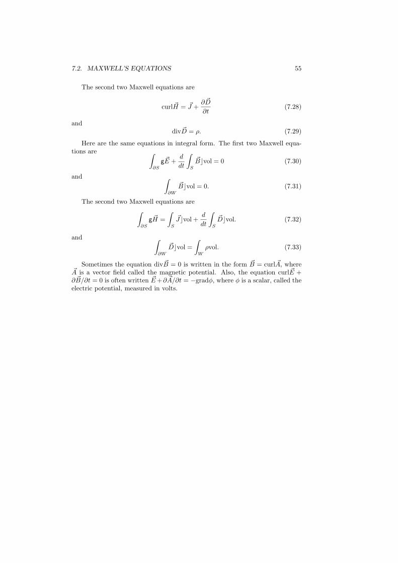
7.2. MAXWELL’S EQUATIONS 55

The second two Maxwell equations are

curl ~H = ~J +∂ ~D

∂t(7.28)

anddiv ~D = ρ. (7.29)

Here are the same equations in integral form. The first two Maxwell equa-tions are ∫

∂S

g ~E +d

dt

∫

S

~Bcvol = 0 (7.30)

and ∫

∂W

~Bcvol = 0. (7.31)

The second two Maxwell equations are∫

∂S

g ~H =∫

S

~Jcvol +d

dt

∫

S

~Dcvol. (7.32)

and ∫

∂W

~Dcvol =∫

W

ρvol. (7.33)

Sometimes the equation div ~B = 0 is written in the form ~B = curl ~A, where~A is a vector field called the magnetic potential. Also, the equation curl ~E +∂ ~B/∂t = 0 is often written ~E+∂ ~A/∂t = −gradφ, where φ is a scalar, called theelectric potential, measured in volts.


7.3 Problems

1. Show that the electric field satisfies

d(εE) = R (7.34)

and∂2E

∂t2+ ε−1dµ−1dE = −ε−1 ∂J

∂t. (7.35)

This is the most important physical conclusion: a static charge producesan electric field; an electric current changing in time produces an electricfield that propagates in space and time.

2. Show that the magnetic field satisfies

dB = 0 (7.36)

and∂2B

∂t2+ dε−1dµ−1B = dε−1J. (7.37)

The electric field changing in space and time is accompanied by a magneticfield changing in space and time.

3. The remaining problems deal with the magnetic and electric potentials Aand ρ. Show that the equations B = dA and E+∂A/∂t = −dφ imply thefirst two Maxwell equations.

4. There is some freedom in how to choose A and φ. Suppose that the choiceis such that dεA = 0. (This is called the transverse gauge condition orCoulomb gauge condition.) Recall that ε may depend on space but noton time, and that it sends 1-forms to 2-forms. Use the fourth Maxwellequation to prove that

dεdφ = −R. (7.38)

This equation shows how the charge 3-form R determines the electricpotential scalar φ.

5. Show that the third Maxwell equation gives

∂2A

∂t2+ ε−1dµ−1dA = ε−1J , (7.39)

whereJ = J − εd∂φ

∂t. (7.40)

Notice that µ−1 may depend on space but not on time, and that it sends2-forms to 1-forms. The equation shows how the 2-form J determines themagnetic potential 1-form A.

6. Suppose again that the transverse gauge condition dεA = 0 is satisfied.Show that the transverse current J satisfies dJ = 0.

Chapter 8

Length and area

8.1 Length

Sometimes it is useful to consider coordinates on a manifold that are not or-thogonal coordinates. The simplest case is that of a two-dimensional manifold.Write the metric as

g = E du2 + 2F du dv +Gdv2. (8.1)

Here E,F,G are functions of u, v. They of course depend on the choice ofcoordinates. What is required is that E > 0, G > 0 and the determinantEF −G2 > 0. When F = 0 we are in the case of orthogonal coordinates.

One way that such a metric arises is from a surface in three-dimensionalspace. Suppose the metric is the usual cartesian dx2 + dy2 + dz2. The lengthof a curve is

s =∫

C

√dx2 + dy2 + dz2. (8.2)

The meaning of this equation is that

s =∫ b

a

√dx

dt

2

+dy

dt

2

+dz

dt

2

dt, (8.3)

where t is a coordinate on the curve, and the end points are where t = a andt = b.

Suppose that the curve is in the surface. Then the length is

s =∫ b

a

√E

(du

dt

)2

+ 2Fdu

dt

dv

dt+G

(dv

dt

)2

dt. (8.4)

Here the coefficients are

E =(∂x

∂u

)2

+(∂y

∂u

)2

+(∂z

∂u

)2

, (8.5)

57

58 CHAPTER 8. LENGTH AND AREA

andF =

∂x

∂u

∂x

∂v+∂y

∂u

∂y

∂v+∂z

∂u

∂z

∂v, (8.6)

and

G =(∂x

∂v

)2

+(∂y

∂v

)2

+(∂z

∂v

)2

. (8.7)

So this gives the explicit formula for the metric on the surface in terms of theequations giving x, y, z in terms of u, v that define the surface. Often one writesthe result for the length of a curve in the surface in the form

s =∫

C

√E du2 + 2F du dv +Gdv2. (8.8)

This just means that one can use any convenient parameter.

8.2 Area

The formula for the area of a surface is

A =∫

S

area =∫

S

√g du ∧ dv =

∫

S

√EG− F 2 du ∧ dv. (8.9)

Here g = EG− F 2 is the determinant of the metric tensor. This is particularlysimple in the case of orthogonal coordinates, in which case F = 0.

There is an alternative expression for the surface area of a surface insideEuclidean space that is sometimes convenient. This is

A =∫

S

area =∫

S

√(dy ∧ dzdu ∧ dv

)2

+(dz ∧ dwdu ∧ dv

)2

+(dx ∧ dydu ∧ dv

)2

du∧dv. (8.10)

Here a fraction such as dy ∧ dz divided by du ∧ dv is a ratio of 2-forms on thesurface S. As we know, such a ration is just a Jacobian determinant of y, z withrespect to u, v.

Bibliography

[1] Ilka Agricola and Thomas Friedrich, Global analysis: Differential forms inanalysis, geometry and physics.

[2] Henri Cartan, Differential forms, Houghton Mifflin, Boston, Massachusetts,1970.

[3] Manfredo P. do Carmo, Differential forms and applications, Springer-Verlag, Berlin, 1994.

[4] Dominic G. G. Edelen, Applied exterior calculus, John Wiley & Sons, NewYork, 1985.

[5] Harold M. Edwards, Differential forms: A differential forms approach,Birkhauser, Boston, 1969.

[6] Luther Pfahler Eisenhart, Riemannian geometry, Princeton UniversityPress, Princeton, New Jersey, 1949.

[7] Harley Flanders, Differential forms with applications to the physical sci-ences, Academic Press, New York, 1963.

[8] John Hamal Hubbard and Barbara Burke Hubbard, Vector calculus, linearalgebra, and differential forms: A unified approach, second ed., Prentice-Hall, Upper Saddle River, New Jersey, 2002.

[9] E. L. Ince, Ordinary differential equations, Dover Publications, New York,1956.

[10] David Lovelock and Hanno Rund, Tensors, differential forms, and varia-tional principles, Dover Publications, New York, 1989.

[11] John Milnor, Morse theory, Annals of Mathematics Studies, no. 51, Prince-ton University Press, Princeton, New Jersey, 1969.

[12] Edward Nelson, Tensor analysis, Princeton University Press, Princeton,NJ, 1967.

[13] , Topics in dynamics I: Flows, Princeton University Press, Prince-ton, NJ, 1969.

59

60 BIBLIOGRAPHY

[14] M. Schreiber, Differential forms: A heuristic introduction.

[15] Michael Spivak, Calculus on manifolds: A modern approach to classicaltheorems of advanced calculus, Addison-Wesley, Reading, Massachusetts,1965.

[16] Gabriel Weinreich, Geometrical vectors, University of Chicago Press,Chicago, 1998.

[17] Steven H. Weintraub, Differential forms: A complement to vector calculus,Academic Press, San Diego, 1997.

Vector elds and di erential forms - Department of...

Documents

Transcript of Vector elds and di erential forms - Department of...