He, F., Zhou, J. and Zhu, H.T. 2003. Autologistic regression model for the distribution of vegetation. Journal of Agricultural, Biological and Environmental Statistics 8:205-222.

Spatial autoregressive modelsSUMBER: www.ualberta.ca/~haitao2/.../ch14.SAR_CAR.ppt

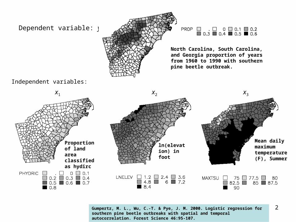
Proportion of land area classified as hydirc

ln(elevation) in foot

Mean daily maximum temperature (F), Summer

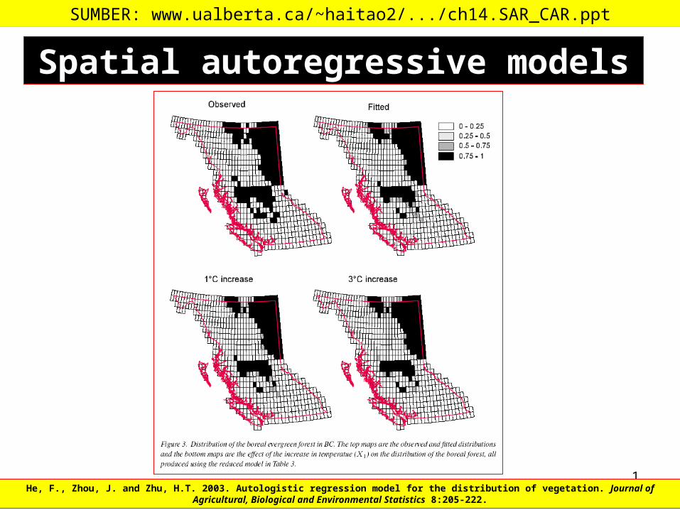
Gumpertz, M. L., Wu, C.-T. & Pye, J. M. 2000. Logistic regression for southern pine beetle outbreaks with spatial and temporal autocorrelation. Forest Science 46:95-107.

Dependent variable: y

North Carolina, South Carolina, and Georgia proportion of years from 1960 to 1990 with southern pine beetle outbreak.

x1 x2 x3

Independent variables:

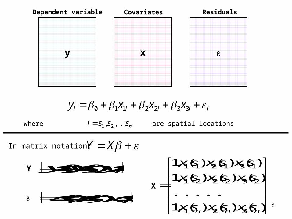
iiiii xxxy 3322110

)(),...,(),( 21 nsysysyY

)(),(),(,1.....

)(),(),(,1)(),(),(,1

321

232221

131211

nnn sxsxsx

sxsxsxsxsxsx

X )(),...,(),( 21 nsss

XY

nsssi ,...,, 21where are spatial locations

In matrix notation:

y x

Dependent variable Covariates Residuals

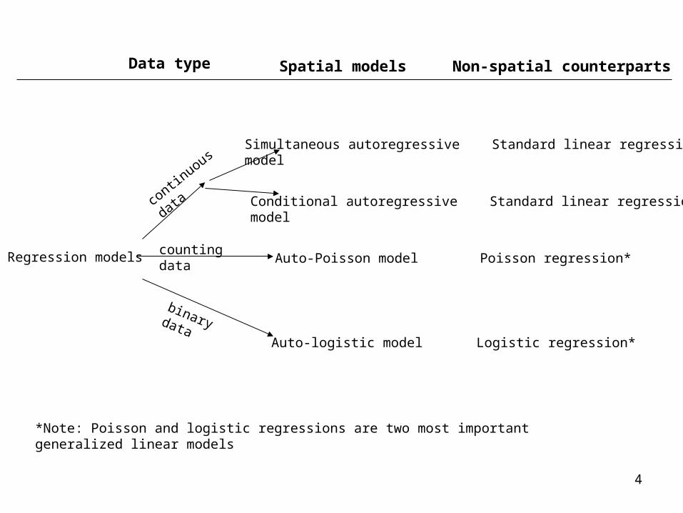
Regression models

contin

uous data

counting data

binary data

Simultaneous autoregressive Standard linear regressionmodel

Conditional autoregressive Standard linear regressionmodel

Auto-Poisson model Poisson regression*

Auto-logistic model Logistic regression*

Data type Spatial models Non-spatial counterparts

*Note: Poisson and logistic regressions are two most important generalized linear models

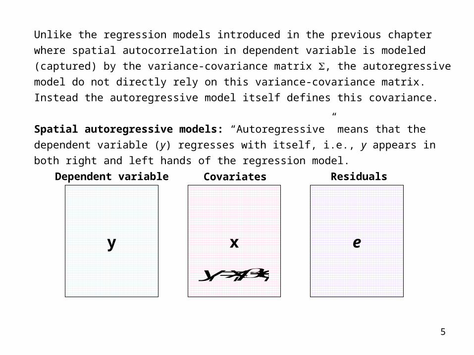
Unlike the regression models introduced in the previous chapter where spatial autocorrelation in dependent variable is modeled (captured) by the variance-covariance matrix , the autoregressive model do not directly rely on this variance-covariance matrix. Instead the autoregressive model itself defines this covariance.

Spatial autoregressive models: “Autoregressive” means that the dependent variable (y) regresses with itself, i.e., y appears in both right and left hands of the regression model.

y x e

Dependent variable Covariates Residuals

iii exy

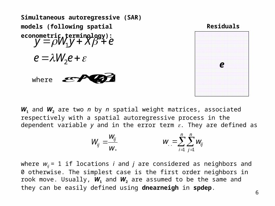
Simultaneous autoregressive (SAR) models (following spatial econometric terminology):

e

Residuals

eWeeXyWy

2

1

..ww

W ijij

),0(~ 2IN where

W1 and W2 are two n by n spatial weight matrices, associated respectively with a spatial autoregressive process in the dependent variable y and in the error term . They are defined as

where wij = 1 if locations i and j are considered as neighbors and 0 otherwise. The simplest case is the first order neighbors in rook move. Usually, W1 and W2 are assumed to be the same and they can be easily defined using dnearneigh in spdep.

n

i

n

jijww

1 1..

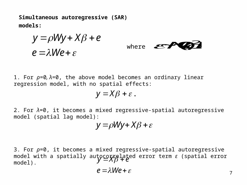
Simultaneous autoregressive (SAR) models:

WeeeXWyy

WeeeXy

),0(~ 2IN where

1. For ρ=0, λ=0, the above model becomes an ordinary linear regression model, with no spatial effects:

2. For λ=0, it becomes a mixed regressive-spatial autoregressive model (spatial lag model):

3. For ρ=0, it becomes a mixed regressive-spatial autoregressive model with a spatially autocorrelated error term ε (spatial error model).

. Xy

XWyy

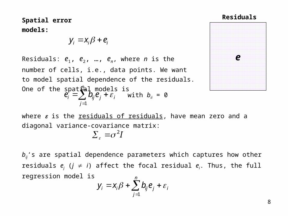
Spatial error models:

e

Residuals

Residuals: e1, e2, …, en, where n is the number of cells, i.e.,

data points. We want to model spatial dependence of the residuals. One of the spatial models is

i

n

jjiji ebe

1

with bii = 0

where is the residuals of residuals, have mean zero and a diagonal variance-covariance matrix:

bij‘s are spatial dependence parameters which captures how other residuals ej (j i)

affect the focal residual ei. Thus, the full regression model is

I2

i

n

jjijii ebxy

1

iii exy

i

n

jjijii ebxy

1

i

n

jjjijii xybxy

1

jjj exy

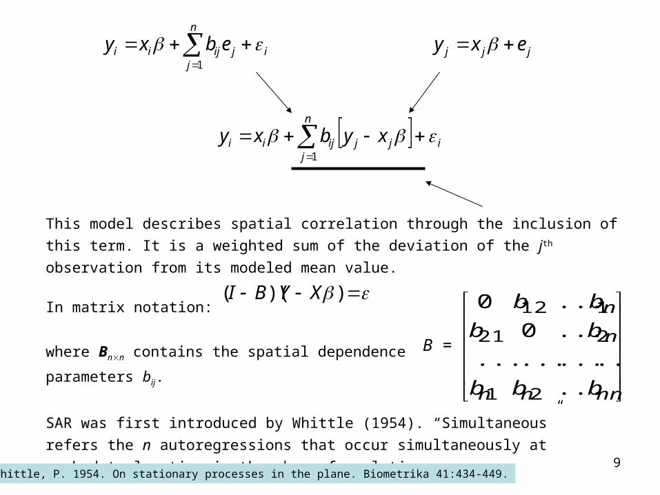
This model describes spatial correlation through the inclusion of this term. It is a weighted sum of the deviation of the jth observation from its modeled mean value.

In matrix notation:

where Bnn contains the spatial dependence

parameters bij.

SAR was first introduced by Whittle (1954). “Simultaneous”refers the n autoregressions that occur simultaneously ateach data location in the above formulation.

))(( XYBI

nnnn

n

n

bbb

bbbb

...............

...0

...0

21

221

112

B =

Whittle, P. 1954. On stationary processes in the plane. Biometrika 41:434-449.

i

n

jjjijii xybxy

1

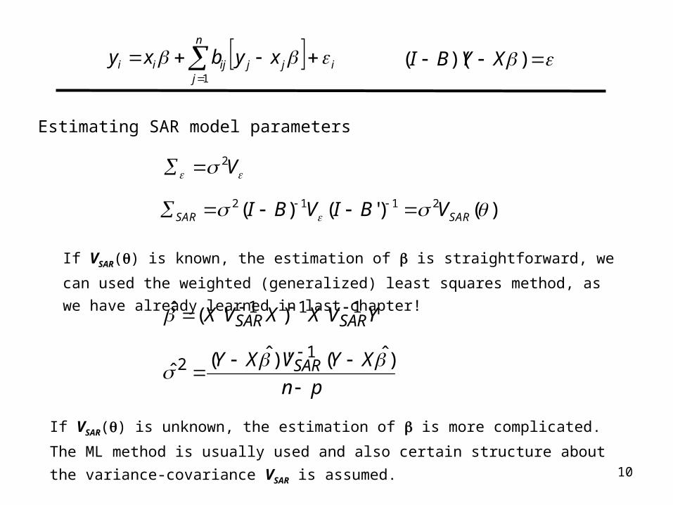
If VSAR() is known, the estimation of is straightforward, we can used the weighted

(generalized) least squares method, as we have already learned in last chapter!

Estimating SAR model parameters

)()'()( 2112 SARSAR VBIVBI

YVXXVX SARSAR111 ')'(ˆ

pnXYVXY SAR

)ˆ()'ˆ(ˆ1

2

If VSAR() is unknown, the estimation of is more complicated. The ML method is usually

used and also certain structure about the variance-covariance VSAR is assumed.

))(( XYBI

V2

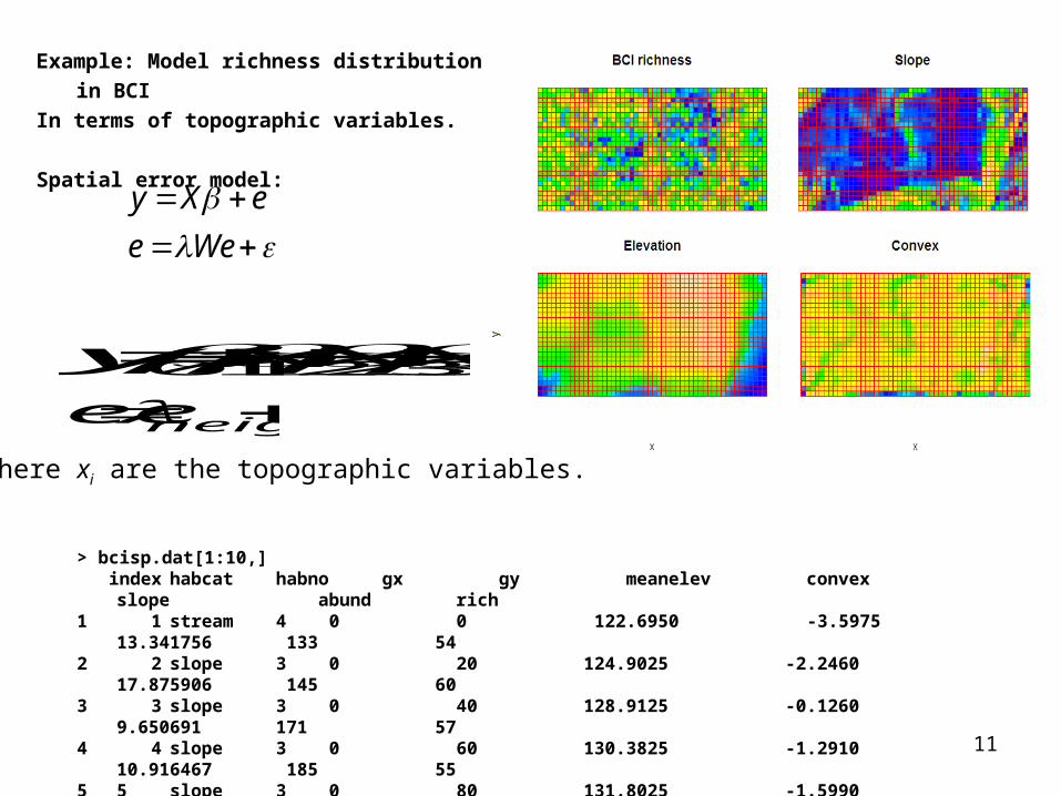
Example: Model richness distribution in BCIIn terms of topographic variables.

Spatial error model:

> bcisp.dat[1:10,] index habcat habno gx gy meanelev convex slope abund

rich1 1 stream 4 0 0 122.6950 -3.5975 13.341756 133

542 2 slope 3 0 20 124.9025 -2.2460 17.875906 145

603 3 slope 3 0 40 128.9125 -0.1260 9.650691 171

574 4 slope 3 0 60 130.3825 -1.2910 10.916467 185

555 5 slope 3 0 80 131.8025 -1.5990 11.921838 185

60….

WeeeXy

exxxy 3322110

neighborsee

where xi are the topographic variables.

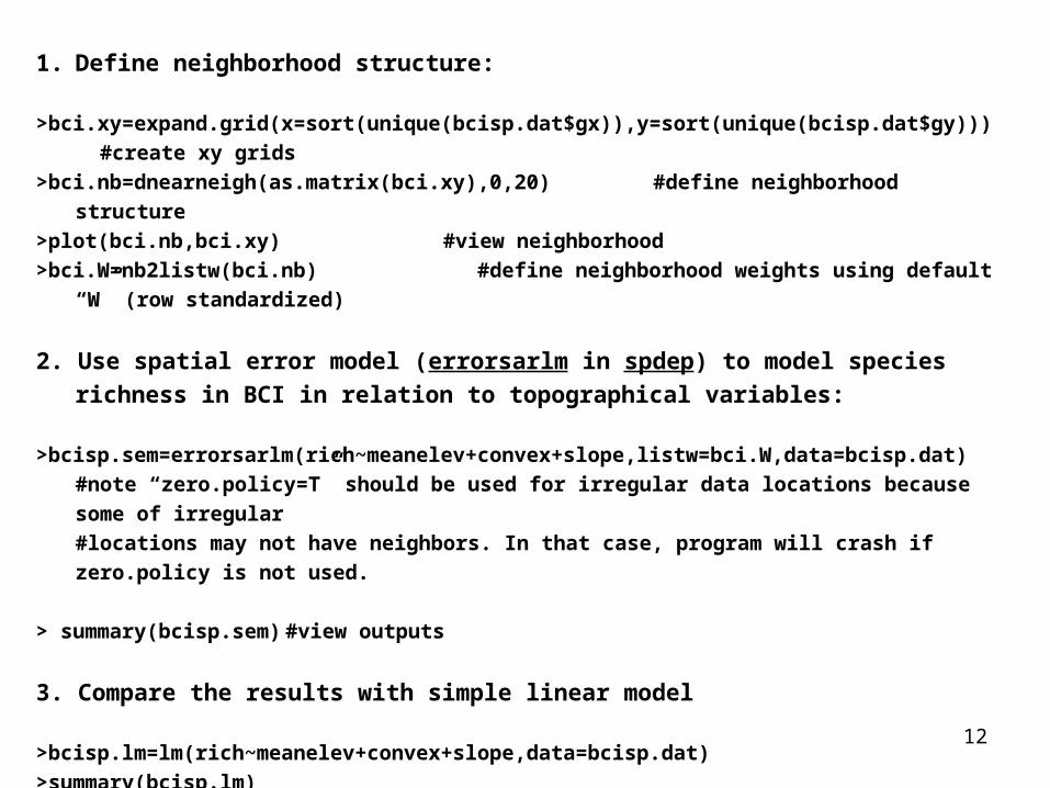
1. Define neighborhood structure:

>bci.xy=expand.grid(x=sort(unique(bcisp.dat$gx)),y=sort(unique(bcisp.dat$gy))) #create xy grids>bci.nb=dnearneigh(as.matrix(bci.xy),0,20) #define neighborhood structure>plot(bci.nb,bci.xy) #view neighborhood>bci.W=nb2listw(bci.nb) #define neighborhood weights using default “W” (row

standardized)

2. Use spatial error model (errorsarlm in spdep) to model species richness in BCI in relation to topographical variables:

>bcisp.sem=errorsarlm(rich~meanelev+convex+slope,listw=bci.W,data=bcisp.dat)#note “zero.policy=T” should be used for irregular data locations because some of irregular #locations may not have neighbors. In that case, program will crash if zero.policy is not used.

> summary(bcisp.sem) #view outputs

3. Compare the results with simple linear model

>bcisp.lm=lm(rich~meanelev+convex+slope,data=bcisp.dat)>summary(bcisp.lm)

Important note: compare both outputs, you will notice that the standard errors for bcisp.sem is larger than those for bcisp.lm

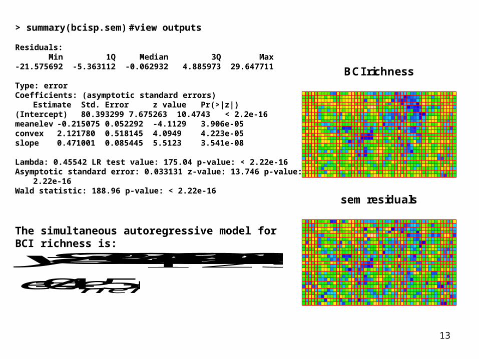
> summary(bcisp.sem) #view outputs

Residuals: Min 1Q Median 3Q Max -21.575692 -5.363112 -0.062932 4.885973 29.647711

Type: error Coefficients: (asymptotic standard errors)

Estimate Std. Error z value Pr(>|z|)(Intercept) 80.393299 7.675263 10.4743 < 2.2e-16meanelev -0.215075 0.052292 -4.1129 3.906e-05convex 2.121780 0.518145 4.0949 4.223e-05slope 0.471001 0.085445 5.5123 3.541e-08

Lambda: 0.45542 LR test value: 175.04 p-value: < 2.22e-16 Asymptotic standard error: 0.033131 z-value: 13.746 p-value: < 2.22e-16 Wald statistic: 188.96 p-value: < 2.22e-16

The simultaneous autoregressive model forBCI richness is:

exxxy 321 471.0122.2215.0393.80

neighborsee 455.0

sem residuals

BCI richness

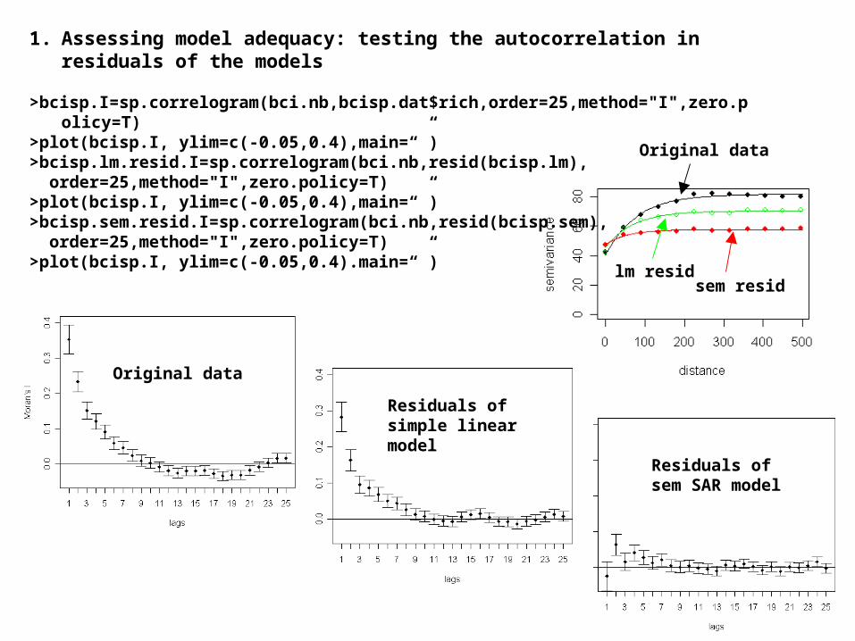
1. Assessing model adequacy: testing the autocorrelation in residuals of the models

>bcisp.I=sp.correlogram(bci.nb,bcisp.dat$rich,order=25,method="I",zero.policy=T)>plot(bcisp.I, ylim=c(-0.05,0.4),main=“”)>bcisp.lm.resid.I=sp.correlogram(bci.nb,resid(bcisp.lm), order=25,method="I",zero.policy=T)>plot(bcisp.I, ylim=c(-0.05,0.4),main=“”)>bcisp.sem.resid.I=sp.correlogram(bci.nb,resid(bcisp.sem), order=25,method="I",zero.policy=T)>plot(bcisp.I, ylim=c(-0.05,0.4).main=“”)

Original data

Residuals of simple linear model

Residuals of sem SAR model

Original data

lm residsem resid

iii yyyyxy 44332211

This defines a joint multivariate normal distribution with

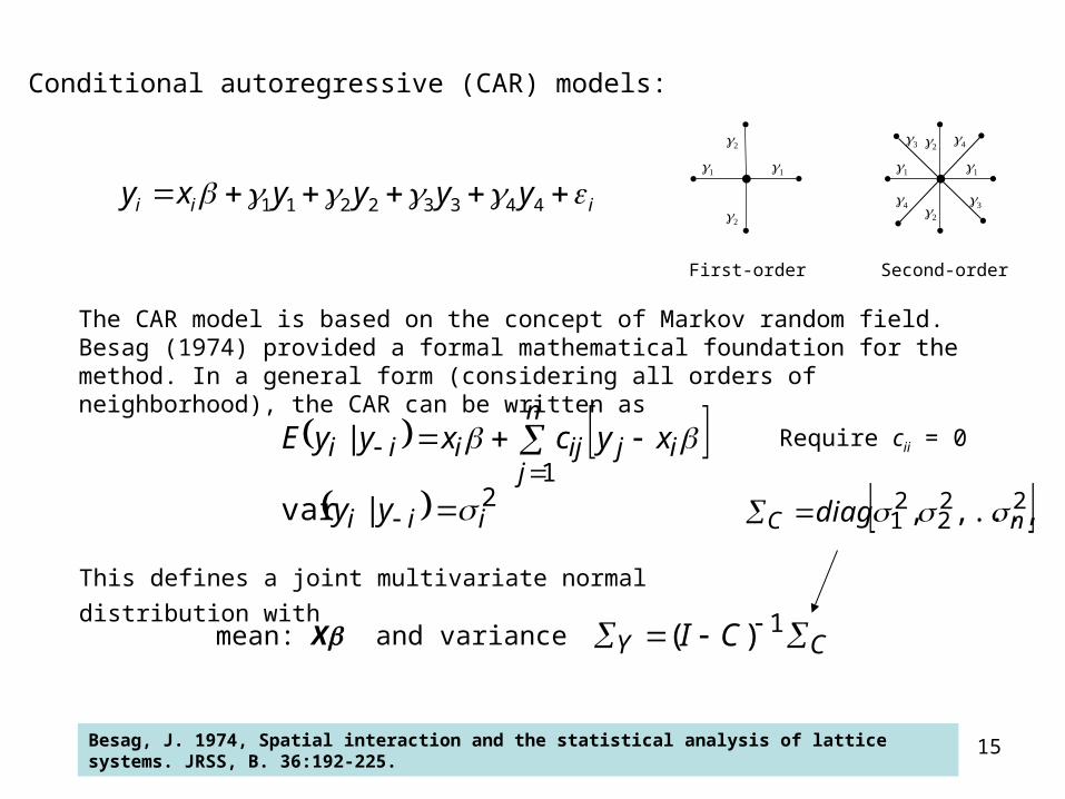
Conditional autoregressive (CAR) models:

11

2

2

First-order

3

3

4

4

Second-order

11

2

2

The CAR model is based on the concept of Markov random field. Besag (1974) provided a formal mathematical foundation for the method. In a general form (considering all orders of neighborhood), the CAR can be written as

n

jijijiii xycxyyE

1|

2|var iii yy

CY CI 1)(mean: X and variance

222

21 ,...,, nC diag

Besag, J. 1974, Spatial interaction and the statistical analysis of lattice systems. JRSS, B. 36:192-225.

Require cii = 0

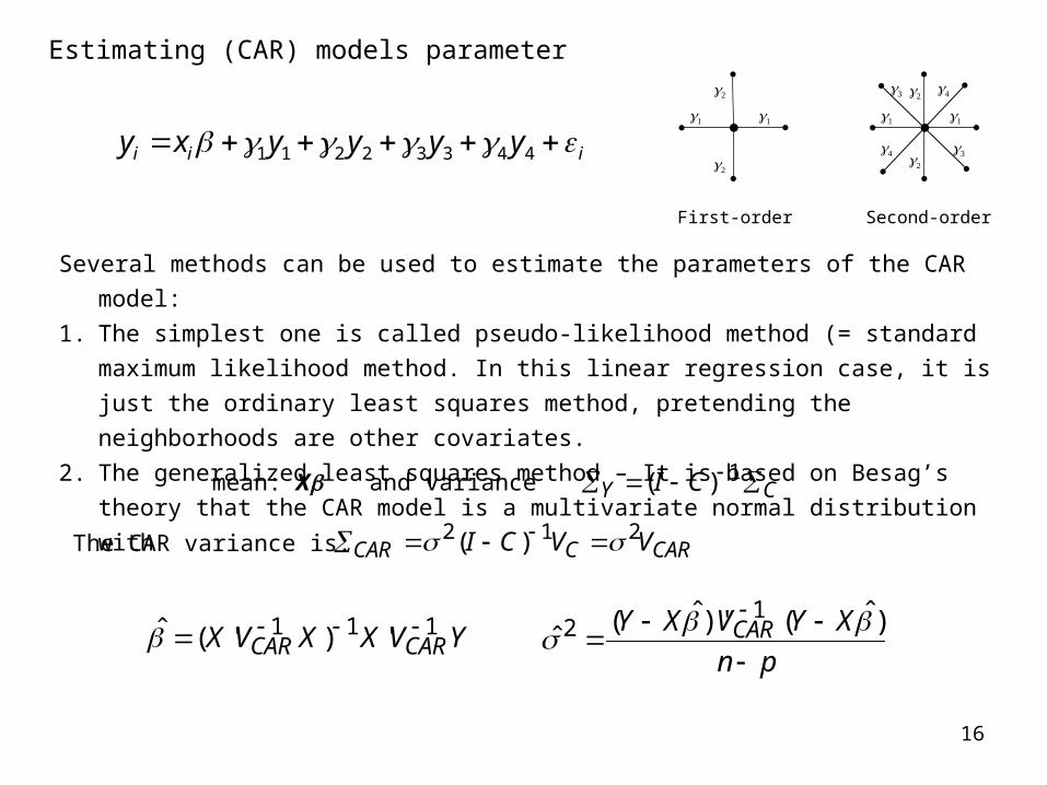
iii yyyyxy 44332211

Several methods can be used to estimate the parameters of the CAR model:1. The simplest one is called pseudo-likelihood method (= standard maximum likelihood

method. In this linear regression case, it is just the ordinary least squares method, pretending the neighborhoods are other covariates.

2. The generalized least squares method – It is based on Besag’s theory that the CAR model is a multivariate normal distribution with

3. MCMC – Markov Chain Monte Carlo simulation algorithm

Estimating (CAR) models parameter

11

2

2

First-order

3

3

4

4

Second-order

11

2

2

CY CI 1)(mean: X and variance

The CAR variance is: CARCCAR VVCI 212 )(

YVXXVX CARCAR111 ')'(ˆ

pnXYVXY CAR

)ˆ()'ˆ(ˆ1

2

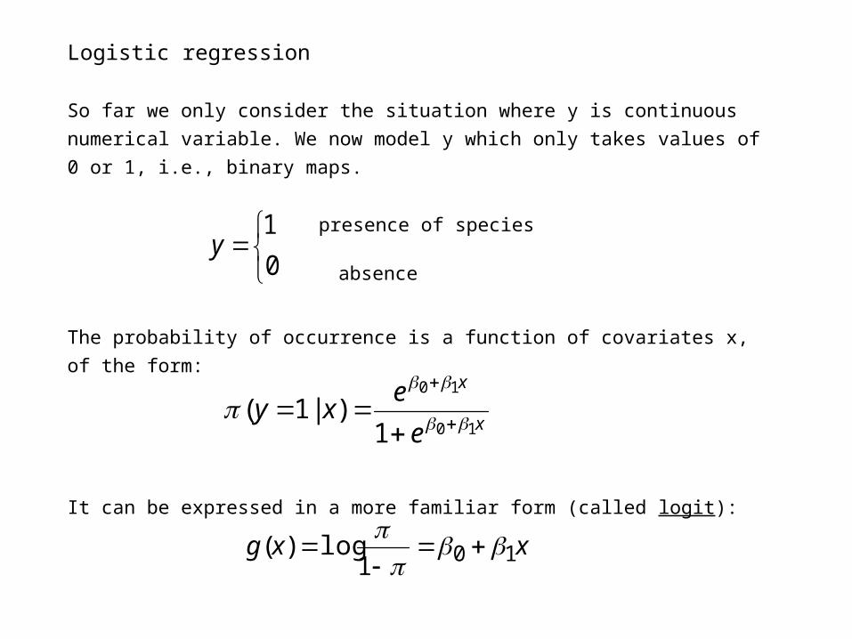
Logistic regression

So far we only consider the situation where y is continuous numerical variable. We now model y which only takes values of 0 or 1, i.e., binary maps.

The probability of occurrence is a function of covariates x, of the form:

It can be expressed in a more familiar form (called logit):

x

x

eexy

10

10

1)|1(

01

ypresence of species

absence

xxg 101log)(

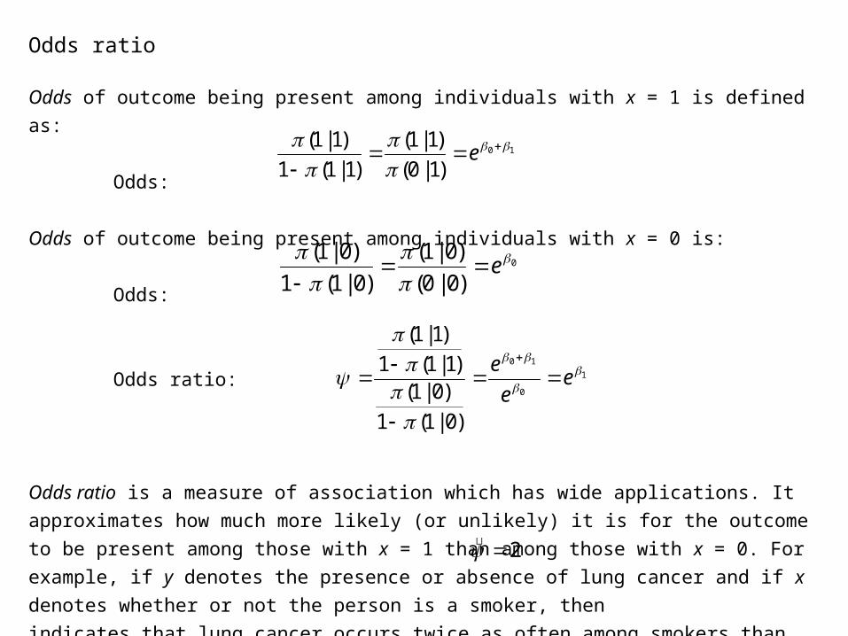
Odds ratio

Odds of outcome being present among individuals with x = 1 is defined as:

Odds:

Odds of outcome being present among individuals with x = 0 is:

Odds:

Odds ratio:

Odds ratio is a measure of association which has wide applications. It approximates how much more likely (or unlikely) it is for the outcome to be present among those with x = 1 than among those with x = 0. For example, if y denotes the presence or absence of lung cancer and if x denotes whether or not the person is a smoker, then indicates that lung cancer occurs twice as often among smokers than among nonsmokers in the study population.

10

)1|0()1|1(

)1|1(1)1|1(

e

0

)0|0()0|1(

)0|1(1)0|1(

e

1

0

10

)0|1(1)0|1()1|1(1

)1|1(

eee

2

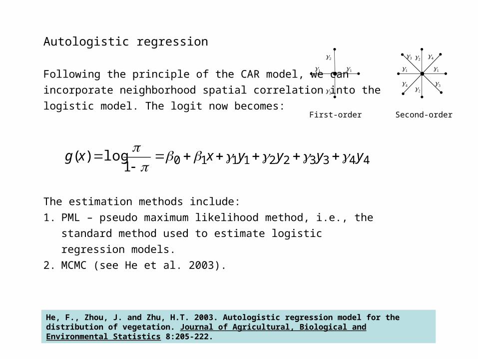
Autologistic regression

Following the principle of the CAR model, we can incorporate neighborhood spatial correlation into thelogistic model. The logit now becomes:

The estimation methods include:1. PML – pseudo maximum likelihood method, i.e., the standard method

used to estimate logistic regression models.2. MCMC (see He et al. 2003).

44332211101log)( yyyyxxg

11

2

2

First-order

3

3

4

4

Second-order

11

2

2

He, F., Zhou, J. and Zhu, H.T. 2003. Autologistic regression model for the distribution of vegetation. Journal of Agricultural, Biological and Environmental Statistics 8:205-222.

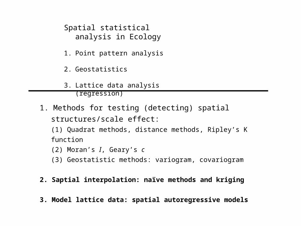
Spatial statistical analysis in Ecology

1. Point pattern analysis

2. Geostatistics

3. Lattice data analysis (regression)

1. Methods for testing (detecting) spatial structures/scale effect:(1) Quadrat methods, distance methods, Ripley’s K function(2) Moran’s I, Geary’s c(3) Geostatistic methods: variogram, covariogram

2. Saptial interpolation: naïve methods and kriging

3. Model lattice data: spatial autoregressive models