Variations of CH4 emissions within and between hydroelectric reservoirs in Brazil

Karin Grandin

Arbetsgruppen för Tropisk Ekologi Minor Field Study 172 Committee of Tropical Ecology ISSN 1653-5634 Uppsala University, Sweden

Oktober 2012 Uppsala

Variations of CH4 emissions within and between Hydroelectric reservoirs in Brazil

Karin Grandin

Supervisors: Dr. Gesa Weyhenmeyer, Department of Ecology and Genetics, Limnology, Uppsala University, Sweden. MSc. Eva Podgrajsek, Department of Earth Sciences, Program for Air, Water and Landscape Sciences, Uppsala University, Sweden. Dr. Luciano de Oliveira Vidal, Laboratory of Aquatic Ecology, Federal University of Juiz de Fora, Brazil. Prof. Fábio Roland, Laboratory of Aquatic Ecology, Federal University of Juiz de Fora, Brazil.

I

ABSTRACT Variations of CH4 emissions within and between three hydroelectric reservoirs in Brazil

Karin Grandin

Hydroelectricity is an energy resource which for a long time has been considered

environmentally neutral regarding greenhouse gas emission. During the last years this view

has changed. Studies have shown that reservoirs connected to hydroelectric power plants emit

methane (CH4) and other greenhouse gases to the atmosphere, especially in the tropical

regions where the emission level of CH4 is the highest. The purpose of this thesis was to

investigate the variations of CH4 emissions in Funil reservoir, Santo Antônio reservoir and

Três Marias reservoir and to identify variables that increase the CH4 emissions.

The CH4 emissions were measured by floating static chambers positioned on the surface at

several locations within each reservoir. A gas sample was collected after 10, 20 and 30

minutes from each chamber. The samples were analyzed through gas chromatography to

obtain the concentration of CH4 in each sample. Calculations of the change in CH4

concentration over time were used to establish the flux of CH4 at each location.

The obtained result from Funil reservoir showed CH4 fluxes in the range of -0.04 to 13.16

mmol/m2/day with significantly different fluxes between sites (p < 0.05). The CH4 fluxes in

Santo Antônio reservoir were within the range of -0.33 to 72.21 mmol/m2/day. In this

reservoir fluxes were not significantly different between sites (p <0.05). The results obtained

from Três Marias showed CH4 fluxes in the range of -0.31 to 0.56 mmol/m2/day with

significantly different fluxes between sites (p < 0.05). The highest fluxes were found in Santo

Antônio which were significantly different from the CH4 fluxes in Três Marias (p <0.05).

The CH4 flux was positively correlated with CO2 and dissolved organic carbon (DOC) and

negatively correlated with O2 and depth in Santo Antônio. The same correlations were evident

for the whole data set. In total the measured fluxes from the three reservoirs ranged from 0.33

to 72.21 mmol/m2/day and the mean flux was 2.31 mmol/m

2/day. These fluxes are low

compared to earlier results. The variation in CH4 flux within and between the reservoirs was

significantly different in a major part of the comparisons. Even though the majority of the

fluxes were different, variables that increase the CH4 emission rate were illuminated. A low

depth and low O2 concentration increase the CH4 emission rate. A high concentration of DOC

and CO2 indicates that a high amount of organic carbon was available for the production of

CH4, leading to an increased CH4 emission rate.

Keywords: CH4 emissions, tropical reservoirs, hydroelectricity, flooded vegetation

Department of Ecology and Evolution, Limnology, Norbyvägen 18 D SE‒752 36 Uppsala,

Sweden

II

REFERAT Variationen av metanemissioner inom och mellan tre hydroelektriska vattendammar i

Brasilien Karin Grandin

Vattenkraft är en energikälla som länge har ansetts vara klimatneutral gällande växthusgaser,

men under de senaste åren har denna bild förändrats. Studier har visat att hydroelektriska

vattendammar avger metan (CH4) och andra växthusgaser till atmosfären och att CH4

emissionerna från dessa dammar är störst i tropiskt klimat. Syftet med detta projekt var att

undersöka variationerna av CH4 emissioner i de hydroelektriska vattendammarna Funil, Santo

Antônio och Três Marias i Brasilien, och att bedöma vilka variabler som påverkar avgången

av CH4 i dessa vattendammar.

För att mäta avgångarna av metan placerades statiska flytkammare på vattenytan på ett antal

platser inom varje vattendamm. Ett gasprov togs efter 10, 20 och 30 minuter från varje

kammare. Gasproverna analyserades genom gaskromatografi och därmed erhölls

koncentrationen av metan i varje prov. Beräkningar av förändringen i koncentration från

början till slutet av mättiden gav metanflödet.

Resultaten från Funil visade signifikant skilda CH4 flöden mellan mätplatser från -0,04 till

13,16 mmol/m2/dag. I Santo Antônio var det lägsta flödet -0,33 mmol/m

2/dag och det högsta

72,21 mmol/m2/dag, och här var flödena mellan mätplatserna ej signifikant skilda. Funil

visade också signifikant skilda flöden mellan mätplatser från -0,31 till 0,56 mmol/m2/dag. De

högsta CH4 flödena erhölls i Santo Antônio, och dessa flöden var signifikant skilda från

flödena i Três Marias. CH4 flödet var positivt korrelerat med CO2 och DOC och negativt

korrelerat med O2 och djup i Santo Antônio. Samma korrelationer gällde för hela

datamängden från de tre vattendammarna tillsammans.

De uppmätta flödena av CH4 från de tre dammarna varierade från -0,33 till 72,21

mmol/m2/dag och medelflödet var 2,31 mmol/m

2/dag. Dessa flöden var låga i jämförelse med

tidigare resultat. Trots att variationen i CH4 flödena var stor inom och mellan vattendammarna

kunde variabler som ökar CH4 emissionerna identifieras. En hög koncentration av CO2 och

DOC indikerade att det fanns stor tillgång på organiskt kol som kunde användas till

produktionen av CH4, vilket ökade emissionerna av CH4. Variablerna O2 och djup hade också

påverkan på CH4 flödet, där ett litet djup och låg O2 koncentration ökade emissionerna av

CH4.

Nyckelord: metanemissioner, tropiska vattendammar, vattenkraft, översvämmad vegetation

Avdelningen för limnologi, Evolutionsbiologiskt Centrum, EBC Norbyvägen 18 D SE‒ 752 36

Uppsala

III

PREFACE This master’s thesis is the last part of the Master of Science program in Aquatic and

Environmental Engineering of 30 ECTS at Uppsala University. It was performed in the spring

semester 2012 and the major part of the thesis was carried out during two months in Brazil.

The thesis was made in cooperation with the Laboratory of Aquatic Ecology at the Federal

University of Juiz de Fora in Minas Gerais, Brazil.

The supervisors of the thesis were Eva Podgrajsek at the Department of Earth Sciences at

Uppsala University and Luciana de Oliveira Vidal at the Laboratory of Aquatic Ecology at the

Federal University of Juiz de Fora in Minas Gerais, Brazil. The subject reviewer was Gesa

Weyhenmeyer at the Department of Ecology and Evolution at Uppsala University.

Sida (the Swedish International Development Agency) together with the Brazilian project

BALCAR were financing this thesis. BALCAR is a project sponsored by Electrobrás, the

Brazilian hydropower agency owned by the government. This thesis would have been

impossible to compass without the financial support from Sida and Electrobrás. In order to

evaluate the obtained results from the performed measurements complementary data were

needed. This data were supplied by several people at the Aquatic Ecology Laboratory in Juiz

de Fora. The results in this study would have been limited without this resource.

First of all I would like to thank Emma Hällqvist, my friend and colleague who performed her

master thesis in connection to mine. Your enthusiasm and your companionship inspired me

during preparations, fieldtrips, lab analyzes and writing. Further on, I would like to thank my

supervisors Eva and Luciana for all the support you have been giving me. Thank you, Eva for

the work you have put into answering my questions and helping me to understand and

practice the method. Thank you, Luciana for your great inputs regarding how to perform the

measurements and also for your help with the logistics connected to the fieldtrips, lab

analyzes and the general stay in Brazil. I wish to thank Nathan Barros for your great advices

regarding how to construct the chambers and how to accomplish the measurements. Thank

you, Rafael Almeida and Felipe Pacheco for your help during the measurements. I also wish

to thank everyone in the Aquatic Ecology Laboratory in Juiz de Fora for making my time in

Brazil an unforgettable experience. Moreover, I would like to thank Giselle Parno Guimaráes

and Alex Enrich Prast who helped me with the GC analyzes in the biogeochemical laboratory

at the federal university of Rio de Janerio. I also wish to thank my subject reviewer Gesa

Weyhenmayer for your great support while I was writing my report, Erik Sahleé and David

Bastviken for the help you have been giving me by answering my questions.

Copyright © Karin Grandin and the Department of Ecology and Evolution, Uppsala University

UPTEC W12 020 ISSN 1401‒5765

Printed at the Department of Earth Sciences, Geotryckeriet, Uppsala University, 2012

IV

POPULÄRVETENSKAPLIG SAMMANFATTNING Vattenkraften är en ständigt växande energikälla som används i hög utsträckning världen

över. I dagsläget har 17 % av de potentiella platserna för vattenkraft utnyttjats. Detta innebär

att det finns mycket utrymme för vattenkraftens framfart. Samtidigt som nya områden

exploateras ökar medvetenheten om de negativa effekterna denna energikälla har på naturen

och klimatet. Vattenkraft anses vara en förnyelsebar energikälla eftersom energin ej kommer

från fossila bränslen utan från naturliga förnyelsebara processer. Hydroelektriska

vattendammar avger trots den förnyelsebara karaktären växthusgaserna koldioxid, metan och

kväveoxid till atmosfären. Dessa gaser avges även vid förbränning av olja, naturgas och kol.

Syftet med den studie som denna rapport baseras på var att se hur utsläppen av metan varierar

inom och mellan tre hydroelektriska vattendammar i Brasilien och vilka faktorer som

påverkar utsläppen.

Metan är en växthusgas som bildas i sedimentet på botten av vattendammar som restprodukt

när bakterier bryter ner organsikt kol. Från att ha tillverkats i sedimentet kan metangasen

antingen stiga upp genom vattnet och avges till atmosfären eller ombildas till koldioxid. Om

vattnet är syrerikt är chansen stor att ombildning till koldioxid sker, medan en låg syrehalt

gynnar utsläpp av metan till atmosfären. Det som främst styr vilken växthusgas som avges är

alltså mängden tillgängligt syre i vattnet, medan produktionen av metan främst styrs av

tillgången på organsikt kol. Utsläppen av metan beror även på ytterligare faktorer som

exempelvis latitud, temperatur, ålder på vattendammen, djup i vattendammen och vattenflöde.

Många av de studier som genomförts har påvisat att de största utsläppen av metan sker i

tropiska områden i jämförelse med tempererade och boreala områden. Detta beror på att dessa

områden påverkas av variabler som är relaterade till höga metanutsläpp i större utsträckning

än områden längre från ekvatorn.

I Brasilien kommer 85 % av energiproduktionen från vattenkraft. En majoritet av

vattenkraftverken är lokaliserad i sydöstra delen av landet vilken är den del där befolkningen

och den industriella verksamheten är som störst. I denna del är taket nått för hur mycket

vattenkraft som får utvinnas. Brasilien är ett land som just nu genomgår en stor ekonomisk

och industriell expansion, vilket medför att energibehovet ökar i samma takt. För att

tillfredsställa den växande energikonsumtionen sker en stor utbyggnad av vattenkraften,

främst i och omkring Amazonas, i den nordöstra delen av landet där 50 % av den totala

vattenkraftspotentialen finns.

För att se hur metanutsläppen varierar och vilka faktorer som påverkar variationen

genomfördes mätningar av metanutsläppen från de tre tropiska vattendammarna Funil, Santo

Antônio och Três Marias i Brasilien. Funil är lokaliserad i sydöstra Brasilien i närheten av Rio

de Janeiro. Denna vattendam har höga halter av näringsämnen eftersom tillrinningsområdet är

tätbefolkat och innehar många industrier. Vattnet är grönt vilket har orsakats av en hög

koncentration av alger. Dessa algerna har producerats på grund av den stora tillförseln av

V

näringsämnen. Santo Antônio ligger i Amazonas vid utkanten av staden Porto Velho. Denna

vattendam är nyligen konstruerad i anslutning till två vattenkraftverk; Santo Antônio och Jirua

som ska börja generera energi 2014. Till följd av byggnationen av vattendammen har stora

landområden med mycket vegetation översvämmats. Três Marias är placerad i mitten av

Brasilien, strax norr om staden Belo Horizonte. Denna vattendamm har klart blått vatten och

en area av 1000 km2.

Mätningarna gjordes genom statiska flytkammare som placerades på vattenytan i

vattendammarna. Tre flytkammare användes på 7 till 13 mätplatser inom varje damm och från

dessa kammare togs luftprover var tionde minut under en halvtimme. De uppmätta proverna

analyserades sedan genom gaskromatografi för att koncentrationen av metan i varje prov

skulle erhållas. När koncentrationen i varje prov var känd kunde metanflödet beräknas genom

hur koncentrationen förändrades med tiden.

Mätningar av metanutsläppen från de tre vattendammarna visade att Santo Antônio hade de

högsta utsläppen av metan och den största spridningen (-0,33‒72,21 mmol/m2/dag) följd av

Funil (-0,04–13,15 mmol/m2/

dag). I Três Marias var utsläppen av metan lägst och spridningen

minst (-0,31–0,56 mmol/m2/dag). I Santo Antonio var utsläppen störst från de områden som

nyligen har översvämmats eftersom det finns en stor tillgång på lättnedbrytbart organsikt

material på dessa platser. Utsläpp av metan skedde även genom vattenväxter. Då

transporterades metan från sedimentet, genom stjälkarna i växterna och upp till atmosfären.

På dessa platser var även syrehalten låg. Funil hade högre metanutsläpp än Três Marias, vilket

troligen berodde på en högre tillgång på organsikt materia och en lägre syrehalt i vattnet. I

Três Marias var metanutsläppen lägst eftersom tillgången på organsikt material var begränsad,

samtidigt som syrehalten var hög.

Det var stor skillnad i metanutsläpp mellan Três Marias och Funil, men också mellan Três

Marias och Santo Antônio. Likheterna i flöde var störst mellan Funil och Santo Antônio.

Trots att metanutsläppen hade stor spridning, kunde variabler som ökade utsläppen

identifieras. En hög koncentration av löst organiskt kol, tillsammans med grunt vatten och låg

syrekoncentration gjorde att utsläppen av metan till atmosfären ökade.

VI

WORDLIST

Allochthonous carbon external carbon that enters an aquatic system

Anoxic low concentrations of O2 in the water

Aquatic boundary

layer

the water layer closest to the surface

Boreal ecosystem located in the sub Antarctic and sub-Arctic regions

DOC Dissolved Organic Carbon

Epilimnion the surface layer of water in a thermally stratified freshwater basin

GHG Green House Gas

Hypolimnion the colder water mass located at the lake floor in a thermally stratified freshwater

basin

Hypoxia too low O2 concentration for the occurrence of oxidation

Lentic areas with still water, like the water in lakes and ponds

Littoral zone the part of a water basin located closest to the shore

Lotic areas with fast moving water, like the water in rivers

Macrophyte a large plant in water vegetation

Monomictic a lake that is entirely mixed once a year

Organic carbon sink where organic carbon is stored, for example in trees

Organic carbon

sources

where organic carbon is released, for example reservoirs

Oxic high concentration of O2 in the water

Riverine zone the zone closest to the inlet of the reservoir which establishes river‒like

characteristics

Temperate ecosystem next to the temperate zone and closer to the equator

TotN Total Nitrogen

TotP Total Phosphorus

Transition zone the zone in a reservoir where the river turns into a lake

Turbidity the cloudiness in the water

Vareza a special kind of rainforest in the Amazon region which is seasonally flooded

Water column a column of water from the lake floor to surface

VII

TABLE OF CONTENTS

ABSTRACT ........................................................................................................................... I

REFERAT ............................................................................................................................. II

PREFACE ............................................................................................................................ III

POPULÄRVETENSKAPLIG SAMMANFATTNING ........................................................ IV

WORDLIST ........................................................................................................................ VI

TABLE OF CONTENTS ............................................................................................ VII

1 INTRODUCTION ...............................................................................................................1

1.1 PROJECT BACKGROUND .........................................................................................1

1.2 PURPOSE .....................................................................................................................2

1.3 LIMITATIONS .............................................................................................................2

2. BACKGROUND ................................................................................................................4

2.1 CH4 IN HYDROELECTRIC RESERVOIRS ................................................................4

2.1.1 Characteristics of CH4.............................................................................................4

2.1.2 How CH4 is created ................................................................................................4

2.1.3 How CH4 is produced, transported and emitted to the atmosphere ...........................5

2.2 VARIABLES DETERMINIG CH4 EMISSIONS ..........................................................7

2.3 BRAZIL ...................................................................................................................... 10

2.3.1 The Brazilian climate ............................................................................................ 10

2.2.2. Hydroelectricity in Brazil ..................................................................................... 11

2.4 PREVIOUS RESULTS REGARDING CH4 EMISSIONS IN THE TROPICS ............ 11

3 METHOD.......................................................................................................................... 12

3.1 STUDY SITES............................................................................................................ 12

3.1.1 Funil reservoir ...................................................................................................... 12

3.1.2 Santo Antônio reservoir ........................................................................................ 13

3.1.3 Três Marias Reservoir ........................................................................................... 15

3.2 THE FLOATING CHAMBER METHOD .................................................................. 17

3.2.1 Measurements ....................................................................................................... 17

3.2.2 Data Analysis ....................................................................................................... 18

3.3 CALCULATIONS ...................................................................................................... 20

3.3.1 Calculating the concentration of CH4 in initial water samples ............................... 20

VIII

3.3 2 Calculating the flux of CH4 ................................................................................... 22

4 RESULTS ......................................................................................................................... 24

4.1 VARIATION IN CH4 FLUXES .................................................................................. 24

4.1.1 Wilcoxon Rank Sum test – Between and within the reservoirs .............................. 27

4.2 VARIABLES .............................................................................................................. 31

4.2.1 Principial component analysis ............................................................................... 33

4.2.2 Correlation analysis .............................................................................................. 36

5 DISCUSSION ................................................................................................................... 37

5.1 FUNIL RESERVOIR. ................................................................................................. 37

5.2 SANTO ANTÔNIO RESERVOIR .............................................................................. 38

5.3 TRÊS MARIAS RESERVOIR .................................................................................... 40

5.4 COMPARISION OF CH4 EMISSIONS ...................................................................... 41

5.5 PRINCIPAL COMPONENT ANALYSIS (PCA) ........................................................ 41

5.6 EXPLAINING VARIABLES ...................................................................................... 43

5.7 LINEAR AND NON‒LINEAR CALCULATIONS OF FLUX.................................... 45

5.8 EVALUATING THE METHOD ................................................................................. 46

5.9 ERRORS ..................................................................................................................... 46

5.10 SUMMARY OF THE RESULTS .............................................................................. 47

6 CONCLUSION ................................................................................................................. 48

7 REFERENCES .................................................................................................................. 49

APPENDIX A ...................................................................................................................... 54

A.1 THE FLOATIONG CHAMBER METHOD ............................................................... 54

A.1.1 Preparation........................................................................................................... 54

A.1.2 In the field ........................................................................................................... 56

A.1.3 Analysis in the lab................................................................................................ 58

APPENDIX B ...................................................................................................................... 60

B.1 MATLAB CODE FOR THE PCA ANALYSIS .......................................................... 60

APPENDIX C ...................................................................................................................... 61

C.3 DATA ........................................................................................................................ 61

1

1 INTRODUCTION Methane, (CH4) is a greenhouse gas with a 23 times higher global warming potential than

CO2. This gas is estimated to be responsible for 20 % of the increased greenhouse effect

observed since the mid 1700s (Bastviken 2009). The amount of CH4 has increased as a

consequence of anthropogenic activities, mainly human waste treatment, cattle ranching and

agriculture, but also by hydroelectric power generation.

Hydroelectric reservoirs contribute to the increased greenhouse effect by emitting CH4 and

other greenhouse gases (GHG) to the atmosphere. The level of emissions can be significant at

a global scale. The emissions, particularly in the tropics, can in some cases be comparable to

the emissions from fossil‒fuel power plants considering GHG emissions per megawatt

produced (Santos et al. 2006). At the moment 17 % of the potential hydroelectric sites are

used globally (Pircher 1993). A major part of the new constructed hydroelectric reservoirs are

built in the tropics, but most of the existing data on GHG emissions are based on

measurements in temperate areas (Roland et al. 2010). Due to this there is a lack of

information regarding the CH4 emissions in the areas currently most exploited, which also are

the areas with highest known GHG emission rate (Louis et al. 2000).

In Brazil, approximately 85 % of the energy supply is generated from hydroelectricity and

most of the hydropower plants are located in the south eastern part of the country. This is the

area where the demand of electricity is the highest due to high population density and intense

industrial activity (Soares et al.2008). In this area the exploitation of hydropower plants has

reached the limit. Further on most of the new constructed hydropower plants are planned to be

situated in the tropic Amazon region (IAEA n.d).

It is important to further investigate the processes that occur within the reservoirs where CH4

is involved, especially in the tropics. Thereby more knowledge will be achieved on how to

locate and construct future hydropower plants and reservoirs in order to minimize the CH4

emission rates. By doing so, hydropower will continue to be considered an environmentally

friendly energy resource.

1.1 PROJECT BACKGROUND

This study was made in cooperation with the Laboratory of Aquatic Ecology at the Federal

University of Juiz de Fora, Minas Gerais, Brazil. At this laboratory a research group is

working with the project BALCAR (Balanço de Carbono) where they perform a large‒scale

field study of the carbon budget in 11 hydropower reservoirs in Brazil. The purpose with the

BALCAR project is to investigate how man‒made hydropower reservoirs affect the carbon

cycle in the prescribed ecosystem, especially the quantity of greenhouse gas emissions. The

main goals within the BALCAR project are:

2

To determine the emissions of greenhouse gases: carbon dioxide (CO2), methane

(CH4) and nitrous oxide (N2O), from the reservoirs.

To identify the pathways of the carbon cycle in these reservoirs, as well as the

environmental factors involved in it.

To evaluate the influence of morphological, morphometric, biogeochemical and

operational variables on the greenhouse gas emissions.

To establish the previous pattern of greenhouse gas emission, prior to the flooding of

the reservoirs.

To develop a spatial and temporal model of the greenhouse gas emissions in reservoirs

that flood Cerrado environments (Cimbleris 2007).

Electrobrás, the Brazilian hydropower agency owned by the government, is financing the

BALCAR project through their three underlying companies FURNAS, ELECTRONORTE

and CHESF. The project was established in order to follow the Brazilian law 9.991/2000. This

law implies that energy producing companies have to make a minimum annual investment of

1% of their net annual revenue in development and research.

The BALCAR project is also performed as a part of the obligations Brazil has as a participant

in the United Framework Convention on Climate Change. The framework convention is an

attempt to handle the problems connected to the increased greenhouse effect, where the aim is

to restrict the concentrations of gases in the atmosphere (Rosa et al. 2002). Brazil thereby

made a commitment when signing this framework to develop and maintain updated

information about the sources and sinks of greenhouse gas emissions, mainly carbon dioxide,

CH4 and nitrous oxide (Cimbleris 2007).

1.2 PURPOSE

The purpose of the thesis was to investigate the variation of CH4 emissions in three different

reservoirs in Brazil and to illuminate the variables that increase the CH4 emission rate. This

was done by comparing the emissions within and between the reservoirs but also by

comparing CH4 emissions with measured variables.

1.3 LIMITATIONS

Several limitations emerged during the project, most of them connected to the short time

available in Brazil, but also limitations regarding the equipment needed to make the

measurements. By spending nine weeks in Brazil, the time used for measurements at the three

reservoirs was relatively short. Therefore, the number of locations used for measurements

3

within each reservoir was few in relation to the size of the reservoirs. At every reservoir

groups of people were making measurements at the same time. Thereby compromises were

done regarding how to perform the measurements. Also the time to do the analyses of the

measured samples in the lab was limited, and due to this the number of analyzed samples was

restricted. The available equipment was limited which also gave rise to limitations.

4

2. BACKGROUND

2.1 CH4 IN HYDROELECTRIC RESERVOIRS

2.1.1 Characteristics of CH4

CH4 is one of the most abundant organic compounds on earth. The gas is colorless and

odorless, melting at -182.5 ⁰ C and boiling at -161.5 ⁰ C. The Henry´s law constant for CH4 at

25⁰ C is 1.29 · 10-3

M atm-1

and this feature gives CH4 low water solubility. CH4 is the main

element in biogas, natural gas and marsh gas and is combustible when 5‒15 % of the air

constitutes of CH4 (Bastviken 2009). CH4 is emitted to the atmosphere by a variety of

anthropogenic and natural sources and the concentration of CH4 in the atmosphere is 1700

parts per billion (ppb) (SLCF 2011). At the same time as CH4 is emitted to the atmosphere the

gas is also degraded there by photo oxidative and hydroxyl radical related processes. The

residence time for CH4 in the atmosphere is 8‒12 years, a short residence time in comparison

to CO2, which has a residence time of 30‒95 years (Jacobson 2005). Due to the short

residence time, a steady‒state increase of CH4 to the atmosphere requires a high amount of

constant emissions from different sources (Bastviken 2009).

2.1.2 How CH4 is created

In hydroelectric reservoirs and other freshwater ecosystems, CH4 is produced in the anoxic

sediment and then released to the water column. Here the gas either gets oxidized or

transported to the water surface where it is emitted to the atmosphere. CH4 is produced in the

sediment from decomposed organic material through methanogenesis, a process performed by

methanogenic archaebacteria. The methanogenesis strictly depends on anoxic conditions and

on a limited number of substrates with low molecular weight. The methanogenesis occurs

mainly through two different pathways; acetotrophic methanogenesis (acetat dependent) and

hydrogenotrophic methanogenesis (H2 dependent). During acetotrofic methanogenesis CH4 is

created by dividing acetate (CH3COO) into CH4 and CO2. In the hydrogenotrophic

methanogenesis a reaction takes place between CO2 and H2 resulting in two components; CH4

and H2O. The most important substrates regarding the methanogenesis are considered to be

acetate, H2 and CO2. Other substrates like formate, methanol, dimethyl sulfide, tri‒, di‒, and

monomethylamines and ethylamine can also be used in the process. The acetotrophic and

hydrogenotrophic methanogenesis most often occur simultaneously. Each process contributes

20‒80% to the overall CH4 production that occures in the sediment.

The performance of methanogenesis depends on a long chain of reactions where organic

matter is the main component eventually liberating the needed substrates. Different bacterial

processes occur in parallel to the methanogenesis and due to this a competition about the

substrate might appear. Depending on current circumstances the methanogenic bacteria can be

concurred out by more efficient substrate uptake systems. These circumstances are affected by

5

different variables, for example pH, Methanogenesis can occur in other parts of the inland

water systems, but the sediment is the main location. This is because this part of the water

systems most often establishes anoxic conditions and also carries large amounts of substrate

(Bastviken 2009).

2.1.3 How CH4 is produced, transported and emitted to the atmosphere

When CH4 is produced in the sediment, it can either get trapped there, or escape towards the

water surface. If CH4 escapes the sediment, it either reaches the water surface and then

diffuses to the atmosphere, or it gets transformed by methano‒oxidizing‒bacteria (MOB)

through oxidation. Oxidation is an energy releasing process performed by methano‒

oxidizing‒bacteria (MOB) with the purpose to make energy available for the bacteria. To

enable oxidation, O2 or another potent oxidant must be available. The MOB can be divided

into three groups with different aims and characteristics, but mutually they all sequentially

oxidize CH4. First into methanol, formaldehyde, formate and then finally CO2. The oxidation

rate is the greatest in connection to the oxic‒anoxic boundary layer where both O2 and CH4

are accessible. This boundary zone exists either in the water column, surface sediment or in

the deeper sediments next to roots liberating O2. The zone where the oxidation arises is

commonly a few millimeters thick if it appears in the sediment. If the oxidation takes place in

the water column the zone is most often thicker, more on a decimeter‒meter scale. The

location of the oxidation zone is controlled by the spatial and temporal variation in O2.

The presence of CH4 highly depends on the oxygen level in the water column. If the water

column is oxic, the main part of CH4 will be oxidized by MOB. If the water column is anoxic

the possibility for CH4 to reach the water surface is high (Bastviken 2009).

CH4 that evades oxidation will escape from the freshwater ecosystem to the atmosphere. This

can happen through three different pathways:

1. Ebullition bubbles that escape from the sediment and quickly transport through the

water column. No oxidation takes place even if the water column is oxic due to the

rapid transportation velocity. The hydrostatic pressure, thereby depth, and the

formation rate of CH4 are main factors that control the amount of CH4 released by

ebullition. It is more common that ebullition bubbles occur at shallow depths due to

the low hydrostatic pressure at these places. Also weather conditions highly affect the

hydrostatical pressure. It has been shown that storms and frontal passages increase the

amount of escaping ebullition bubbles because the air pressure gets lower (Abril et al.

2005).

2. Diffusive flux between the air and surface water. The transportation is caused by

processes of turbulent enhanced diffusion. Due to the low speed of the diffusive

released CH4, oxidation can occur especially in oxic water layers or sediments.

6

Thereby the amount of CH4 released through diffusion highly depends on the oxygen

level in the water column. Since CH4 has a low solubility in water most freshwater

systems are oversaturated in CH4. This means that the diffusive flux, mainly driven by

concentration differences and turbulence, most often will emit CH4 to the atmosphere

because of the oversaturation (Rosa et al. 2004).

3. Flux through macrophytes. Aquatic plants can emit CH4 to the atmosphere from

their leaves. CH4 is transported from the sediment to the leaves through the stems of

the plant by using the transportation system that normally transports O2. This process

can be passive or driven by pressure differences depending of the species of the

macrophytes (Bastviken 2009).

In reservoirs two additional pathways exist due to the man‒made artificial influence on the

ecosystem.

4. Degassing downstream the reservoir. Due to the turbulence the turbines cause on the

water transported downstream the reservoir, extended amounts of CH4 can be emitted

to the atmosphere straight after the dam (UNESCO/IHA 2009).

5. Increased diffusive flux along the river downstream. Further downstream the same

kind of diffusive flux will occur as the diffusive flux upstream. The downstream flux

will be higher because of the turbulence that still appears in the water.Theese

emissions can occur 10 meters to 50 km downstream (UNESCO/IHA 2009).

Figure 1 The different pathways of CH4 emissions connected to hydroelectric reservoirs.

7

The major part of the open water CH4 emissions come from plants and ebullition bubbles,

where approximately 50 % is caused by ebullition. This number should be considered

together with the fact that ebullition is the pathway most difficult to quantify. The probability

that these emissions are underestimated is high due to lack of measured data (Bastviken

2009).

The CH4 emissions highly depend on the characteristics of a reservoir. Reservoirs have

limnological properties representative for both rivers and lakes (Thornton 1990). There is a

common longitudal pattern observed in many reservoirs where the upper part of the reservoir

has characteristics similar to a river, while the lower part is more comparable with a lake (De

Freitas Terra et al. 2010). A longitudal pattern can appear in reservoirs caused by lotic

influences, and lead to a creation of three distinct zones defined by their biological, chemical

and physical characteristics.

The riverine zone, which is the zone closest to the river, is defined by a high inflow of

nutrients where the primary production is low because of the high turbidity. The transition

zone appears afterwards when the water moves further into the reservoir. In this zone the

sedimentation rate and light availability increase and as a consequence the primary production

gets higher. The lentic zone is at the end of the reservoir, close to the dam. The high

sedimentation rate in this area limits the primary production.

Several features affect the size and borders between these zones, like water retention time,

morphometric, thermal stratification and latitude. The variable that affects the zonation the

most is the retention time. If the retention time is short, a great part of the reservoir comprises

the riverine zone (Soares et al. 2008).

2.2 VARIABLES DETERMINIG CH4 EMISSIONS

The processes of producing, transporting and emitting CH4 rely on many different variables.

These variables altogether determine the rate of CH4 production, rate of oxidation and also the

present pathways. The opinions about which variables that affect the CH4 emissions the most

vary. Many articles are pointing at the importance of latitude, climate, dissolved organic carbon

and age of reservoir in connection to the CH4 emissions (Barros et al. 2011; Rosa et al.

2002).The most important variables are described below.

Depth

The depth is an important variable regarding whether CH4 in the sediment will be released or

not since CH4 emissions are controlled by the hydrostatical pressure. The hydrostatic pressure

is often low in shallow parts of a reservoir. It is thereby easier for CH4 gas to overcome the

hydrostatical pressure in these areas compared to deeper areas, resulting in ebullition release.

8

Dissolved oxygen

The amount of oxygen in the water has a great influence on whether CH4 will be transported

to the surface or if it will go through oxidation on its way up. The limiting level where a water

body is considered to establish hypoxic condition is at the oxygen concentration of 2‒3 mg/L

(Kalff 2002).

Turbulence, turbidity and retention time

The direction and speed of the water flow within a reservoir affects the processes where CH4

is involved. A short retention time is a result of high water speed and this condition obstructs

the sedimentation of incoming organic material. This results in a loss of substrate that could

have been used in the methanogenesis process. The water speed and direction also affect the

oxidation process. A high turbulence increases the mixing of the water, and this can generate

a more oxic water body. But the mixing can also ease the release of CH4 to the atmosphere by

moving water, with a high concentration of CH4 located close to the sediment, upwards.

Turbulence also exposes a larger surface area to the atmosphere which enables an increase in

the flux of CH4 (Bastviken 2009). The CH4 emissions that are released downstream the dam

are highly affected by the turbulence. It is thereby difficult to conclude whether turbulence

increases or decreases the CH4 emissions, because it varies depending on the current

circumstances. Turbulence most often occurs as a consequence of certain weather conditions

such as wind and rain, or in connection to the dam and the turbines.

Dissolved organic carbon

Organic carbon has an important role regarding the production of CH4. However, the

composition of the available organic carbon is more important than the quantity. Unstable

organic carbon, like litter and leaves decompose quickly, while older, more stable organic

carbon, such as organic matter and peat, decompose slowly. When a reservoir is constructed

flooded organic material is transferred into the reservoir and a big part of the organic carbon

is easily decomposable organic carbon (Louis et al. 2000). In younger reservoirs, less than 15

year old, the flooded biomass stands for the major part of the organic carbon source (Barros et

al. 2011). Tree boles need very long time to decompose when they are found in flooded areas

because the lignin that is decomposed by fungi cannot be decomposed due to the surrounding

water (Louis et al. 2000). The amount of allochthonous organic carbon transferred into the

reservoir also affects the emission rate (Louis et al. 2000). Climate type and surrounding

vegetation thereby have great impact on the CH4 emissions since type and quality of the

allochthonous organic carbon transferred into the reservoir affect the CH4 emission rates.

9

Age of reservoir

The age is an important variable that affects the emissions. Because of differences in

decomposable organic carbon access, younger reservoirs emit more CH4 than older reservoirs.

When a reservoir starts to get older the emission rate first decreases exponentially and then

decrease with time (Barros et al. 2011).

Concentration of total phosphorus and total nitrogen

The concentration of total phosphorus (total P) and total nitrogen (total N) affect CH4

emission since the primary production, controlled by these nutrients, is the source of organic

material in the sediment. The primary production rate depends on the available amount of

these nutrients, and more organic material is created if great loads of phosphorus and nitrogen

are present. Thereby more organic material is transferred to the sediment ready to be

decomposed which will increase the produced amount of CH4.

Temperature

The decomposition of organic carbon is high in the tropics due to the high annual mean

temperature in the water (Louis et al. 2000). The optimal temperature for methanogenesis is

around 30 ⁰C in the sediment (Jones et al. 1982) and if the temperature increases with 10⁰C

the potential production rate of CH4 is increasing fourfold (Conrad 2002). CH4 oxidation rates

seem to be less sensitive to temperature changes than methanogenesis, but high light intensity,

which can be coupled to temperature, inhibits the CH4 oxidation (Bastviken 2009).

Latitude

Latitude is assumed to affect the amount of emissions due to differences in climate type and

temperature (Rosa et al. 2002). The temperature brings energy to the whole ecosystem, which

determines the rates of the processes within the system. The climate type determines the load

of allochthonous organic material that enters the reservoir.

pH

When the pH level in a lake is within a normal pH interval this variable does not seem to

affect the methanogenesis. But a small change in pH within the normal interval might affect

the composition of substances available for the process. Thereby the methanogenesis is

affected indirectly. The optimal pH for the methanogenesis process is 5‒6 (Zinder 1993).

When the pH is low acetotrophic methanogenesis seems to be the dominant one and when pH

is high the hydrogenotrophic methanogenesis is favored. No clear pattern has been observed

between pH and the CH4 oxidation rates. A reason for this might be the ability the microbal

communities locally adapt to various pH intervals (Bastviken 2009).

10

Dam construction

The ways of operating a hydropower plant highly affect the CH4 emissions from the reservoir.

The energy generation occurs when water passes the turbines, and depending on the

placement of the water outlet and the position of the turbines the amount of emissions

downstream varies. If the outlet is located at a great depth there is a high risk that the water

will bring CH4 through the outlet which will cause degassing emissions (UNESCO/IHA

2009). Also the difference in water level caused by the energy generation affects the

emissions. If the water level is low for a long time, new vegetation will grow along the shore.

When the water level raises this vegetation will be flooded and transferred into a part of the

load of easily decomposed organic material in the reservoir. The hydrostatical pressure in the

reservoir is affected when there is a change in water level, which may lead to releases of

ebullition bubbles (Louis et al. 2000).

2.3 BRAZIL

2.3.1 The Brazilian climate

CH4 emissions from reservoirs highly depend on the climate, because the climate affects a

number of other variables that are connected to the CH4 processes. Major parts of Brazil are

located on or close to the equator and this placement causes a tropical climate and high

atmospheric humidity. The Amazon lowland and surrounding areas receive more than 2000

mm of rain annually. The annual rainfall in the rest of Brazil is approximately 1000‒1500

mm. In Brazil several different biomes re represented, but the ones that covers most of the

land are the semi‒arid “Sertão”, the rain forest “Foresta”, the low and bushy shrubs called

“Caatinga” and the savanna and grassland called “Cerrado”. The Sertão exist in the inner

north‒eastern part and frequently suffers from droughts. The Foresta is found in the

surrounding of the Amazon basin, and the Cerrado is the biome in great parts of the south and

south‒east of Brazil. The Caatiga is situated in the inner north‒east. There are three major river

systems in Brazil; the Amazon in the north, the São Francisco in the east and the Parana‒

Paraguay‒Plata in the south. The Amazon is the second longest river in the world (6440 km) and

the major river in South America (IAEA s.a). Most hydro power plants and reservoirs in Brazil

are situated in the south‒east region. The biome in this area mostly consists of Cerrado and the

climate is categorized as humid‒tropic. The three reservoirs used for this study are located in

different biomass and different river systems. Funil reservoir is located in the Cerrado and is a

part of the Parana‒Paraguay‒Plata River system, Santo Antônio is situated in the Foresta in the

Amazon basin and Três Marias is situated in the Cerrado and the São Francisco River system. All

three reservoirs are situated in the tropical region.

11

2.2.2. Hydroelectricity in Brazil

Brazil is the fifth largest country in the world in area and has one of the largest hydroelectric

potentials worldwide. Most of the potential has not yet been exploited but the hydroelectric

resources in the south, south‒east and north‒east have already been thoroughly used. To feed

the growing need of energy the north and central west regions, where the Amazon is situated

are starting to get exploited (IAEA s.a). About 50% of the hydroelectric potential of Brazil is

located in the Amazon basin (Braga et al. 1998).

At the moment Brazil is going through a great expansion period regarding hydropower. In the

late 90s the energy department of the Brazilian government compiled a program called “plan

2015” where a decision was made about constructing 424 new hydroelectric dams during the

period 2000‒2015. In 2009, 50 of these had been constructed and at that time 70 more were

projected. So far about 2200 large dams have been constructed in Brazil (120 in Sweden) and

more than 3.5 million hectares have been flooded (Naturskyddsföreningen 2009).

2.4 PREVIOUS RESULTS REGARDING CH4 EMISSIONS IN THE TROPICS

Studies of the CH4 emissions in tropical flooded areas started in the eighties, and the

Amazonian area and the African forest were the first regions that were surveyed (Rosa et al.

2002). Many studies have been focusing on this topic since then. Here are some examples and

the obtained results of the CH4 fluxes in the studies.

Batlett et al. (1993) studied flooded vegetation, both with and without floating vegetation.

The measurements varied between 0.47 mmol/m2/day and 60.27 mmol/m

2/day and the mean

flux was 12.47 mmol/m2/day.

Hamilton et al. (1995) investigated the Pantanal wetland of Brazil. 540 samples were taken in

this savanna floodplain region, where the sampling areas consisted of sheet flooding, marsh

streams and the major river in the area. The calculated mean diffusive CH4 flux in the air‒

water interphase was 14.65 mmol/m2/day.

Galy‒Lacaux et al. (1997) analyzed the CH4 flux rate in the Petit Saut reservoir, located on

the Sinnamary River in French Guinea, South America. The mean fluxes of diffusion during

the study ranged from 7.5 mmol/m2/day to 202 mmol/m

2/day. The measurements occurred

over a two year period, between 1994 and 1995 and the measurements started when the

reservoir was filled with water and 300 km2 were flooded. During the 2 years, 10% of the

carbon stored in the reservoir was released to the atmosphere as CH4.

12

3 METHOD

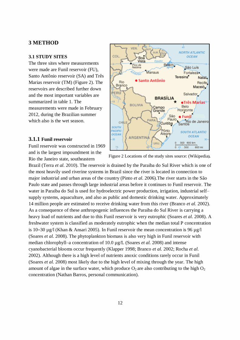
3.1 STUDY SITES

The three sites where measurements

were made are Funil reservoir (FU),

Santo Antônio reservoir (SA) and Três

Marias reservoir (TM) (Figure 2). The

reservoirs are described further down

and the most important variables are

summarized in table 1. The

measurements were made in February

2012, during the Brazilian summer

which also is the wet season.

3.1.1 Funil reservoir

Funil reservoir was constructed in 1969

and is the largest impoundment in the

Rio the Janeiro state, southeastern

Brazil (Terra et al. 2010). The reservoir is drained by the Paraiba do Sul River which is one of

the most heavily used riverine systems in Brazil since the river is located in connection to

major industrial and urban areas of the country (Pinto et al. 2006).The river starts in the São

Paulo state and passes through large industrial areas before it continues to Funil reservoir. The

water in Paraiba do Sul is used for hydroelectric power production, irrigation, industrial self‒

supply systems, aquaculture, and also as public and domestic drinking water. Approximately

14 million people are estimated to receive drinking water from this river (Branco et al. 2002).

As a consequence of these anthropogenic influences the Paraiba do Sul River is carrying a

heavy load of nutrients and due to this Funil reservoir is very eutrophic (Soares et al. 2008). A

freshwater system is classified as moderately eutrophic when the median total P concentration

is 10‒30 µg/l (Khan & Ansari 2005). In Funil reservoir the mean concentration is 96 µg/l

(Soares et al. 2008). The phytoplankton biomass is also very high in Funil reservoir with

median chlorophyll‒a concentration of 10.0 µg/L (Soares et al. 2008) and intense

cyanobacterial blooms occur frequently (Klapper 1998; Branco et al. 2002; Rocha et al.

2002). Although there is a high level of nutrients anoxic conditions rarely occur in Funil

(Soares et al. 2008) most likely due to the high level of mixing through the year. The high

amount of algae in the surface water, which produce O2 are also contributing to the high O2

concentration (Nathan Barros, personal communication).

Figure 2 Locations of the study sites source: (Wikipedia).

13

Funil reservoir is located in the Brazilian Cerrado biome (savannah) and the general climate is

tropical. The soil in the Cerrado biome is poor and overlies the pre‒cambrium rock (Roland et

al. 2010).

There is a limited amount of vegetation in the area surrounding the reservoir as a result of

previous agriculture used for coffee plantations and pasture (Terra et al. 2010). A major part

of this vegetation consists of planted eucalyptus trees. The company supplying the energy,

Electrobras Furnas, has settled a reforestation program in the area surrounding the reservoir

with the purpose to restore the forest (Terra et al. 2010). The operation water level ranges

from 444 m.a.s.l. to 465.5 m.a.s.l. during the year, which means that the water level varies

about 15 m. This water fluctuation causes no further erosion or sedimentation in the reservoir

(Terra et al. 2010).

Funil reservoir has a long and wide section in

the middle of the reservoir where the origin is

the Paraiba do Sul River. This part is

connected to two branches: one from the

Santana tributary and the other one from the

Lajes tributary (Branco et al. 2002). The

reservoir basin follows the typical spatial

zonation described above (riverine‒

transitional‒lentic), where variation in light

availability and nutrients in the sediment is

the reason for the zonation (Soares et al.

2008). In the riverine zone the predominant substrate is clay and the average depth is 4 m. In

the transition zone the substrate is mostly consisting of stones and rocks and the average depth

is 11 m. The depth in the lentic zone is about 20 m and the sediment consists of sand (Terra et

al. 2010).

The Secchi depth is low in the whole reservoir, but lowest in the riverine zone and highest in

the transitional zone and the lentic zones. The lower value in the riverine zone appears due to

the turbidity and inflow of suspended material. The transparency increases in the transition

zone and lentic zone because of the decreased turbidity and inflow of suspended material

(Branco et al. 2002; Terra et al. 2010).

3.1.2 Santo Antônio reservoir

Santo Antonio reservoir is located in the Amazon region in the northwestern part of Brazil

next to the city of Porto Velho (Figure 2). The reservoir is mainly a part of the Madeira River,

but also the tributaries Jaci‒paraná and Jatuarana and the reservoir has more riverine

characteristics than lake characteristics. There are two hydroelectric power plants in this part

of the river: the Santo Antonio dam and the Jirau dam. At the moment these hydroelectric

Figure 3 The green water in Funil reservoir.

14

power stations are under construction but are planned to be ready to generate energy in 2014

(Odebrecht 2012). The two power plants will together produce 6.450 megawatt (MW) of

electricity, and thereby become the third largest hydropower complex in the country (Leite et

al. 2011). In order to minimize the flooded area, a “run of river” system is constructed, where

low head bulb turbines will rotate by the natural speed and flow of the river. This system does

not need a large fall height of water to generate energy, which results in a minimized flooded

area. 44 low‒head bulb turbines will be used at each of the two power plants (Santo Antônio

Energia 2009). The purpose of building these two power stations is to support the southern

parts of Brazil with energy resulting in a 2500 km long transmission corridor (Switker &

Bonilha 2008).

Areas next to the shore of the Madeira River, Jaci‒Paraná and Jatuarana have been flooded

during the construction of the power stations. Part of this flooding is natural and varies

depending on season but the flooding is to a certain extent man‒made. The Madeira River

was half the size before the reservoir was constructed. In Jatuarana the width of the tributary

has increased from approximately 10 m to about 100 m since it became a part of the reservoir

(Rafael Almeida, personal communication)(Figure 4).Some of the flooded areas are

deforested while several others are covered with vegetation. On many places this vegetation

has not been removed before the flooding, and therefore large amounts of organic material

have been transported into the reservoir. The water is very dark in those flooded areas where

no deforestation has occurred, due to the high amount of flooded organic material and also

because of the material the drainage area brings into the flooded parts (Castillo et al. 2004).

Gas bubbles are visible at many places in the tributaries (Figure 5).

The Madeira River is a so called white river which means that the river has a white color

caused by the high amount of suspended material transported by the water. The origin of the

water and the suspended material is the sedimentary and morphometric rocks in the Andes

(Stallard & Edmond 1983; Lyons & Bird 1995) and in the pre‒Cambrian and Cenozoic

sediments that are present in the catchment area (Junk et al. 2011). This geologic structure

together with seismic phenomena in the Andes, soils vulnerable to erosion, a river with

Figure 4 Bubbles in a tributary in Santo

Antônio.

Figure 4 Flooded road in Jatuarana.

15

unstable sandbanks and heavy rainfall contribute to the great load of suspended material

(Carvalho et al. 2011). The Madeira River is carrying nearly half the load of the sediments

and nutrients transported from the Amazon region into the Atlantic Ocean (Latrubesse et al.

2005). This makes Madeira River the principal contributor to the life and diversity of the

Amazon (Switker & Bonilha 2008). The Secchi depth is very low in the river as a

consequence of the high amount of suspended material in the water (about 10 cm), both

downstream and in the reservoir. This result in a low ability for the sunlight to penetrate the

water and thereby almost no cyanobacteria can be found in the river. The few existing

phytoplankton are quickly transported downstream due to the short retention time in the river

and tributaries (Rafael Almeida, personal communication). The suspended material is

deposited in várzeas, a local name for large floodplains. These areas are highly productive

and covered with aquatic and terrestrial plants and floodplain forests (Junk et al. 2011).

Madeira River is draining geologically recently formed terrains and the high amount of

suspended material transported in the Madeira River is a consequence of that (Rafael

Almeida, personal communication).

3.1.3 Três Marias Reservoir

Três Marias reservoir is located in the northern part of the state of Minas Gerais (Figure 2)

and is mainly drained by the São Fransico River, but also the tributaries S. Vicente,

Paraopeba, Extrema, Sucurúi, Ribeirão do Boi, Borrachudo and Indaiá (Fonseca et al. 2007).

The purpose of building the dam was flood control, flow regulation and hydropower

generation and the construction work ended in 1960. Since then this reservoir is one of the

largest artificial lakes in Brazil (Arantes et al. 2011). The reservoir is oligotrophic and

monomictic where the mixing event takes place in July in the dry season due to a high wind

speed. It is stratified when the temperature difference between the hypolimnion and

epilimnion is greater than 3 degrees and this occurs during the wet season between November

and February (Carolsfeld et al. 2003).

Mixing events can also appear in the wet

season because of rain, but the reservoir is

most often stratified (Felipe Pacheco,

personal communication). The dry winter

and the rainy summer cause a high intensity

of soil and rock weathering and this enables

soluble elements to leach into the drainage

basin, most commonly happening between

October and April (Fonseca et al. 2007).

Três Marias reservoir is set in the Cerrado,

the Brazilian savannah, and this area has

been a subject to deforestation during the

Figure 5 The blue-green water in Três Marias

reservoir.

16

last decades. Native species have been replaced by eucalyptus and large cattle ranches and

over‒erosion of soil has become a problem within the reservoir and tributaries (Sampaio &

Lopez 2003 in Brito et al. 2011). The soluble elements and the eroded soil turn into

suspended material and when this material is transported to the outlet of the reservoir it gets

trapped behind the dam. The accumulated sediment load causes major environmental and

technical problems such as filling the reservoir and thereby changing the characteristics. The

tributaries Borrachudo and Indaiá are the main contributors to the high sediment load

(Fonseca et al. 2007). The water level in the reservoir varies 2 – 5 meters within a year and

the water level is the lowest in October‒ November. This is because water is released through

the dam during this time period to enable water to flow in when the wet season starts in

December. Water is dammed during the wet season to enable energy generation during the

dry season (Felipe Pacheco, personal communication).

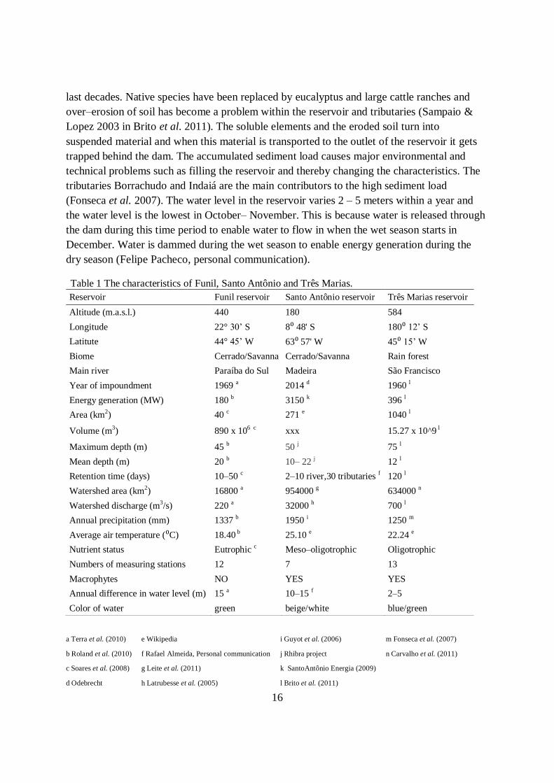
Table 1 The characteristics of Funil, Santo Antônio and Três Marias.

Reservoir Funil reservoir Santo Antônio reservoir Três Marias reservoir

Altitude (m.a.s.l.) 440 180 584

Longitude 22° 30’ S 8⁰ 48' S 180⁰ 12’ S

Latitute 44° 45’ W 63⁰ 57' W 45⁰ 15’ W

Biome Cerrado/Savanna Cerrado/Savanna Rain forest

Main river Paraíba do Sul Madeira São Francisco

Year of impoundment 1969 a 2014 d 1960 l

Energy generation (MW) 180 b 3150 k 396 l

Area (km2) 40 c 271 e 1040 l

Volume (m3) 890 x 106 c xxx 15.27 x 10^9 l

Maximum depth (m) 45 b 50 j 75 l

Mean depth (m) 20 b 10‒ 22 j 12 l

Retention time (days) 10‒50 c 2‒10 river,30 tributaries f 120 l

Watershed area (km2) 16800 a 954000 g 634000 n

Watershed discharge (m3/s) 220 a 32000 h 700 l

Annual precipitation (mm) 1337 b 1950 i 1250 m

Average air temperature (⁰C) 18.40 b 25.10 e 22.24 e

Nutrient status Eutrophic c Meso‒oligotrophic Oligotrophic

Numbers of measuring stations 12 7 13

Macrophytes NO YES YES

Annual difference in water level (m) 15 a 10‒15 f 2‒5

Color of water green beige/white blue/green

a Terra et al. (2010) e Wikipedia i Guyot et al. (2006) m Fonseca et al. (2007)

b Roland et al. (2010) f Rafael Almeida, Personal communication j Rhibra project n Carvalho et al. (2011)

c Soares et al. (2008) g Leite et al. (2011) k SantoAntônio Energia (2009)

d Odebrecht h Latrubesse et al. (2005) l Brito et al. (2011)

17

3.2 THE FLOATING CHAMBER METHOD

3.2.1 Measurements

The method that was used to measure the CH4 emissions from the water surface to the

atmosphere was the floating chambers method. This method is further described in the

UNESCO/IHA measurement specification guidance for evaluating the GHG status of man‒

made freshwater reservoirs (UNESCO/IHA 2009). The measurements were done by the use

of three floating chambers placed on the water surface at every measurement location. Initial

gas samples were taken with syringes from the air and water in the surrounding of the

chambers. A syringe was connected to a hose on top of each chamber and gas was collected

after 10, 20 and 30 minutes from every chamber. Each gas sample was transferred from the

syringe to a vial. The samples in the vials were then analyzed by the use of gas

chromatography (GC) to obtain the concentration of CH4 in each gas sample. The

concentrations of CH4 in the initial samples and in the samples from the chambers were used

to calculate the flux of CH4 emissions to the atmosphere. A more detailed description

regarding how the measurements were performed is available in appendix A.

The spatial measurements in Funil were distributed in 12 stations located to make the best

possible representation of the whole reservoir. The water level was very low when the

measurements took place and reddish clay was exposed in the littoral zone due to the low

water level. The water in the whole reservoir was very green (Figure 3), and the color was

most evident at the stations close to the inlet of the reservoir. Also a lot of visible garbage was

floating around in the reservoir, mostly close to the inlet, so it is clearly understandable that

the reservoir receives much material that affects the ecosystem within the reservoir. The

measurements were made during the rainy season in the summer and normally this time of the

year a thermal stratification appears in this reservoir (Soares et al. 2008). No macrophytes

were observed.

The measurements in Santo Antônio reservoir were made at 7 different stations in the

reservoir. Three stations were situated in the river while the other four were situated in the

tributaries. One tributary station was used to measure emissions from macrophytes.

Measurements were also made downstream at three different places, two in the river and one

in a small bay. The water level differs 12 meters during the year and the level was high when

the measurement took place (approx. 3 m below the highest level) but the water level would

increase until March and then decrease. Erosion was visible almost everywhere next to the

shore downstream and could easily be seen. Macrophytes occurred at many places both

upstream and downstream the reservoir.

Measurements were made at 13 stations in the Três Marias reservoir. Also temporal

measurements were made close to the shore to measure how the amount of CH4 increased

during 36 hours. The water level was high because the measurements were taken in the wet

season. Phytoplankton and zooplankton can easily be seen in the water all over the reservoir

18

and thereby the color of the water is green‒blue (Figure 6). Macrophytes also exist at

numerous places in the reservoir.

3.2.2 Data Analysis

The concentrations of CH4 in the samples obtained from the gas chromatography were used to

calculate the fluxes of CH4 at every station. The fluxes were calculated by a linear

approximation and a non‒linear function (described further down), and the fluxes that were

used for the continued analyzes were based on the non‒linear function. These analyzed fluxes

were obtained from the three chambers at each station after 30 minutes deployment time. The

fluxes obtained after 10 and 20 minutes deployment time were not used in the analysis

because they were unreliable. Therefore 36 fluxes were used in the results from Funil (12

stations x 3 chamber) and 39 (13 stations x 3 chambers) from Três Marias. In Santo Antonio

19 measurements were used (6 stations x 3 chambers + 1). The additional single flux came

from the control chamber at station 7 with the macrophytes.

The differences in CH4 fluxes within and between the reservoirs were statistically calculated

with the Wilcoxon Rank Sum Test. This test compares the median value between two

populations of data and calculates whether the data are significantly different or not. The test

is based on the null hypothesis “means are equal” where the significance limit is 0.05. The

populations are considered equal when the significance (P) is above 0.05 (the null hypothesis

cannot be rejected, H=0), and significantly different when the significance (P) is below 0.05

(the null hypothesis can be rejected, H=1). The obtained flux data did not have a normal

distribution and this is why this test was used.

A principal component analysis (PCA) was performed in Matlab to detect the combined effect

of variables on CH4. The central idea of PCA is to reduce the number of dimensions in a

dataset, where related variables form one dimension. The method creates a reduced set of

variables, where each new variable is a linear combination of the original variables. The new

variables are so called principal components (Mathworks 2012). The PCA displays the

variables in a coordinate system and how they are related to each other. Variables that are

situated close to each other are related. If variables are situated in the diagonal opposite

quadrant they affect the system in a different direction. Variables that are located in

quadrants next to each other do not have any strong relationship. The result from a PCA can

also be displayed in a table.

The PCA was made by loading 15 chosen variables (CH4 flux, CH4 concentration in chamber

samples, depth, concentration of dissolved O2 in the water, concentration of CO2 in the water,

air temperature, concentration of DOC, water temperature, wind speed, total N

concentrations, total P concentration, chlorophyll‒a concentration, pH) into the workspace as

a matrix. The variables in the matrix were log‒transformed to put them in a normal

19

distribution. The matrix was also standardized in order to pay regard to the different units

among the variables. The used command was stdr. The principal components were then

found by the command primcomp. A m‒file was created with the code to generate a plot of

the PCA with the 1st component on the x‒axis and the 2

nd component on the y‒axis which

displayed the scores and the loadings. An additional plot of the explanation in the variance for

each component was generated. One PCA was constructed for the whole dataset representing

the three reservoirs, and one PCA for each reservoir. The outliers were included in the dataset

when the PCA were performed. The stations with missing data were excluded in the analysis.

The strongest relationships between CH4 flux and the variables in the PCA were analyzed by

correlation analyses in Matlab. The correlation analysis displayed positive correlations,

negative correlation and no correlation between CH4 and the different variables based on the

significance (P) and explanation degree (R). A value of P below 0.05 and a value of R close to

1 indicated a positive correlation, while a value of P below 0.05 and value of R close to -1

indicated a negative correlation.

20

3.3 CALCULATIONS

The flux of CH4 was calculated by two different methods; a linear approximation and a non‒

linear function for diffusive flux (David Bastviken, personal communication).

3.3.1 Calculating the concentration of CH4 in initial water samples

To be able to calculate the CH4 flux by the non‒linear function, the concentration of CH4 in

the initial water sample was calculated by the ideal gas law together with measurements from

the gas chromatography (GC). In order to calculate the initial concentration of CH4 in the

water the amount of CH4 compound in the initial air sample (n) and in the initial water sample

(ntot) was determined.

In the air sample the amount of compound was calculated by

n

(1)

where:

n = amount of compound in air sample (moles)

V = volume of air, 0.060 L

R = gas constant = 0,082056 (L atm K-1

moles-1

)

T = temperature of air (K)

P = partial pressure of CH4 in air sample (atm)

and

(2)

where

ppmaamples= concentration (ppm) of CH4 in air sample obtained from the GC

Ptot = total atmospheric air pressure (atm).

The total atmospheric air pressure, Ptot varies depending on the altitude. Ptot at a certain

altitude can be calculated by

(

) (3)

where

h = altitude above sea level (m).

In the water sample the amount of compound was divided into two parts; gas headspace (ng)

and water headspace (nH2O), which together equal the amount of CH4 compound in the water

sample (ntot).

The amount of compound in the gas phase (ng) was calculated by equations 1 and 2 where

21

n = amount of compound in headspace gas of water sample (moles)

V = volume of gas in headspace, 0.020 L

T= temperature of water (K)

P= partial pressure of CH4 in gas phase (atm)

ppmsample= concentration (ppm) of CH4 in gas headspace in water sample obtained from GC.

Henry´s law was used to calculate the amount of compound in the water headspace

(4)

where

CH2O= concentration of CH4 in water (M)

PH2Ohead= partial pressure of CH4 in water headspace (atm)

Kh= Henry´s law constant (M atm-1

).

PH2O was calculated by equation 2 where the concentration (ppm) of CH4 in the gas phase in

the water sample was obtained from the GC.

The amount of compound in the water phase was calculated by

(5)

where

nH2O = amount of compound in headspace water of water sample (moles)

VH2O = volume of water in headspace, 0.040 L.

The total amount of compound in the water sample was given by

(6)

and the initial concentration of CH4 in the water was calculated by

(7)

22

3.3 2 Calculating the flux of CH4

The flux of CH4 can be calculated in a simplified way by the use of a linear approximation. It

can also be calculated by a non‒linear function, which imitates the flux of CH4 in a chamber

better than the linear approximation. CH4 can only be emitted until the air in the chamber is

saturated in CH4, since the chamber limits the area where the diffused CH4 can occur. The

non‒linear function takes into account the decrease in flux over time that occurs when the

diffusion is getting closer towards equilibrium. Since the flux decreases with time a linear

approximation will underestimate the flux of CH4. Therefore the non‒linear function gives a

more accurate result than the linear approximation when measurements are done over a longer

time.

Linear approximation

The linear approximation of the flux was obtained by using the initial CH4 concentration in

the air and the end CH4 concentration in the chamber together with the ideal gas law.

The initial partial pressure of CH4 was approximated by the partial pressure of CH4 in the

initial air sample calculated by equation 2. The partial pressure of CH4 in the chamber sample

at the end of the deployment time was also calculated by equation 2.

The formula for the flux was transformed together with equation 1

( ( ))

( )

( ) (8)

where

F= flux (moles m-2

d-1

)

A= bottom area of chamber (m2)

V= chamber volume (L)

T= air temperature (K)

tend-tinit= the deployment time (days)

ninit = initial amount of compound during deployment time

nend = end amount of compound during deployment time.

Non‒linear diffusive flux

When calculating the non‒linear diffusive flux the following equation was used

( ) (9)

where

k= gas transfer velocity (m d-1

)

23

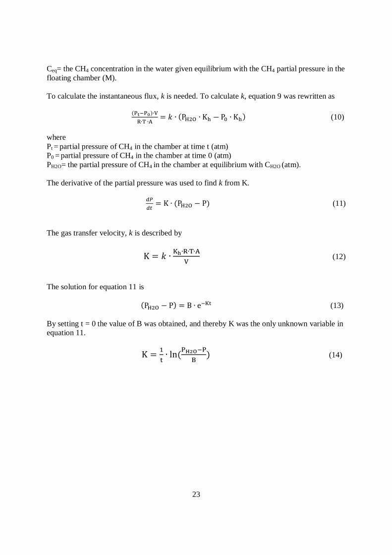
Ceq= the CH4 concentration in the water given equilibrium with the CH4 partial pressure in the

floating chamber (M).

To calculate the instantaneous flux, k is needed. To calculate k, equation 9 was rewritten as

( )

( ) (10)

where

Pt = partial pressure of CH4 in the chamber at time t (atm)

P0 = partial pressure of CH4 in the chamber at time 0 (atm)

PH2O= the partial pressure of CH4 in the chamber at equilibrium with CH2O (atm).

The derivative of the partial pressure was used to find k from K.

( ) (11)

The gas transfer velocity, k is described by

(12)

The solution for equation 11 is

( ) (13)

By setting t = 0 the value of B was obtained, and thereby K was the only unknown variable in

equation 11.

(

) (14)

24

4 RESULTS

4.1 VARIATION IN CH4 FLUXES

The CH4 fluxes displayed on the maps constitute mean values taken from the three chambers

at each station after 30 minutes deployment time. The fluxes in Funil ranged from 0.01

mmol/m2/day to 0.65 mmol/m

2/day, except from station 7 (5.75 mmol/m

2/day) and station 9

(9.97 mmol/m2/day)

The highest mean CH4 fluxes in Santo Antônio were found at station 2 (39.6 mmol/m2/day), 5

(16.13 mmol/m2/day) and 7 (36.44/7.56 mmol/m

2/day). Station 7 showed higher flux from

macrophytes (36.44 mmol/m2/day) than from the control chamber (7.56 mmol/m

2/day). The

remaining mean fluxes were within the range -0.27 mmol/m2/day – 0.42 mmol/m

2/day.

Figure 7 Funil reservoir: measurement stations and their mean CH4 fluxes after 30 minutes

deployment time.

Figure 8 Santo Antônio reservoir: measurement stations and their mean CH4 fluxes after 30 minutes

deployment time.

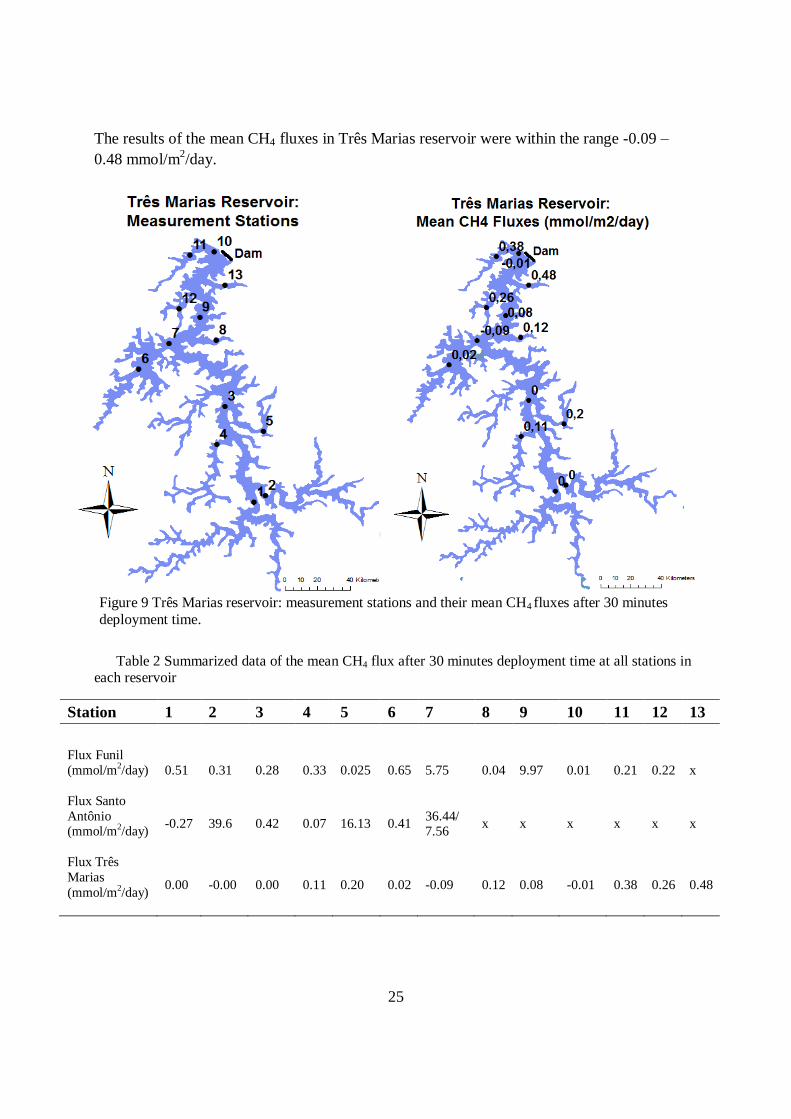
25

The results of the mean CH4 fluxes in Três Marias reservoir were within the range -0.09 –

0.48 mmol/m2/day.

Table 2 Summarized data of the mean CH4 flux after 30 minutes deployment time at all stations in each reservoir

Station 1 2 3 4 5 6 7 8 9 10 11 12 13

Flux Funil

(mmol/m2/day)

0.51 0.31 0.28 0.33 0.025 0.65 5.75 0.04 9.97 0.01 0.21 0.22 x

Flux Santo

Antônio (mmol/m2/day)

-0.27 39.6 0.42 0.07 16.13 0.41 36.44/ 7.56

x x x x x x

Flux Três

Marias

(mmol/m2/day)

0.00 -0.00 0.00 0.11 0.20 0.02 -0.09 0.12 0.08 -0.01 0.38 0.26 0.48

Figure 9 Três Marias reservoir: measurement stations and their mean CH4 fluxes after 30 minutes

deployment time.

26

The CH4 fluxes in Santo Antônio had the highest maximum, median, mean, standard

deviation and variance (Table 3). The CH4 fluxes in Funil had a higher maximum, median,

mean, standard deviation and variance than Três Marias. Santo Antônio had a wide range

regarding the variability in flux with 25% of the measurements within an approximate range

of 0 – 15 mmol/m2/day and one major outlier (Figure 10). Funil had a more narrow range of

CH4 fluxes, but three outliers are observed in the boxplot. The fluxes in Três Marias were

concentrated in a small range and no outliers were found. These results were based on the

CH4 fluxes obtained at 30 minutes deployment time from all chambers at each station in every

reservoir (Table 3, Figure 10). This is why the min and max differ from the earlier mentioned

results (Figure 7, 8 , 9, Table 2).

Table 3 The CH4 flux variability within each reservoir. regarding min, max, median, mean, standard

deviation, variance and number of samples. Data based on the CH4 fluxes measured in all chambers at 30 minutes deployment time.

Reservoir Min Max Median Mean STD Var n

Flux Funil (mmol/m2/day) -0.04 13.15 0.27 0.99 2.68 7.20 36

Flux Santo Antônio (mmol/m

2/day)

-0.33 72.21 0.46 9.30 17.68 312.5 19

Flux Três Marias

(mmol/m2/day)

-0.31 0.56 0.08 0.12 0.20 0.04 36

Flux All (mmol/m2/day) -0.33 72.21 0.21 2.31 8.71 75.88 91

Figure 10 The boxplots display the variability in CH4 flux within the reservoirs with all chamber measurements obtained at 30 minutes deployment time.

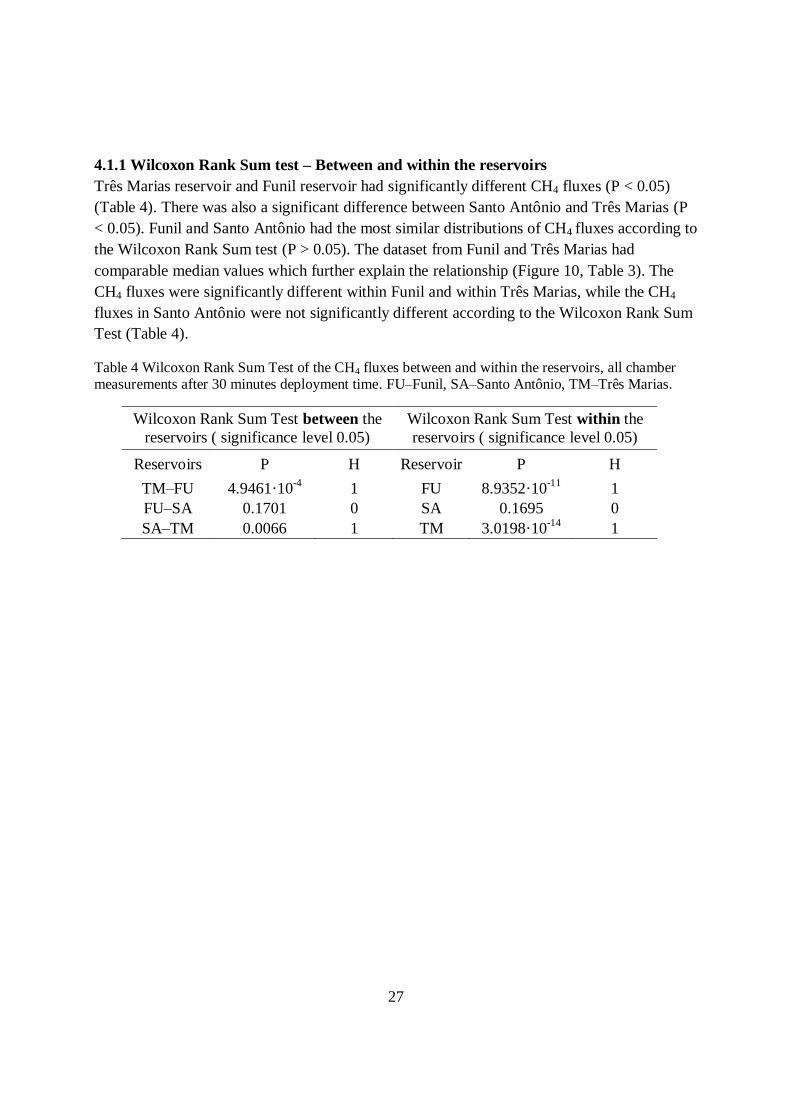
27

4.1.1 Wilcoxon Rank Sum test – Between and within the reservoirs

Três Marias reservoir and Funil reservoir had significantly different CH4 fluxes (P < 0.05)

(Table 4). There was also a significant difference between Santo Antônio and Três Marias (P

< 0.05). Funil and Santo Antônio had the most similar distributions of CH4 fluxes according to

the Wilcoxon Rank Sum test (P > 0.05). The dataset from Funil and Três Marias had

comparable median values which further explain the relationship (Figure 10, Table 3). The

CH4 fluxes were significantly different within Funil and within Três Marias, while the CH4

fluxes in Santo Antônio were not significantly different according to the Wilcoxon Rank Sum

Test (Table 4).

Table 4 Wilcoxon Rank Sum Test of the CH4 fluxes between and within the reservoirs, all chamber measurements after 30 minutes deployment time. FU‒Funil, SA‒Santo Antônio, TM‒Três Marias.

Wilcoxon Rank Sum Test between the

reservoirs ( significance level 0.05)

Wilcoxon Rank Sum Test within the

reservoirs ( significance level 0.05)

Reservoirs P H Reservoir P H

TM‒FU 4.9461·10-4

1 FU 8.9352·10-11

1

FU‒SA 0.1701 0 SA 0.1695 0

SA‒TM 0.0066 1 TM 3.0198·10-14

1

28

There was a much greater concentration of CH4 in the initial water sample (blue), than in the

initial air sample (green) at most stations (Figures 11). Two exceptions where the initial air

sample had a higher concentration were station 8 and 9 in Santo Antônio. These stations were

situated downstream the reservoir. The mean CH4 flux (black line) was generally high at

stations where the concentration of CH4 in the water was high. The greatest exception was

station 9 in Funil. The flux at this station was very high even though there was a low

concentration of CH4 in the water. The graph of Santo Antônio shows no flux at station 8, 9

and 10. The water at these stations was very turbulent and chamber measurements could not

be done due to this and thereby no fluxes were obtained.

-0,1

0,0

0,1

0,2

0,3

0,4

0,5

0,6

-2

0

2

4

6

8

10

12

1 2 3 4 5 6 7 8 9 10 11 12 13

CH

4 F

lux (

mm

ol/

m2

/da

y)

Init

ial C

H4

con

cen

tra

tion

(p

pm

)

Station

Três Marias

0

1

2

3

4

5

6

7

0

5

10

15

20

25

30

1 2 3 4 5 6 7 8 9 10 11 12C

H4 F

lux (

mm

ol/

m2/d

ay)

Init

ial C

H4 c

on

cen

trati

on

(p

pm

)

Station

Funil

0

5

10

15

20

25

30

35

40

45

0

10

20

30

40

50

60

70

1 2 3 4 5 6 7 8 9 10

CH

4 F

lux (

mm

ol/

m2

/da

y)

Init

ial C

H4 C

on

cen

trati

on

(p

pm

)

Stations

Santo Antônio

Figure 11 The concentration of CH4 in initial water and air samples in Funil, Santo Antônio and Três Marias.

29

The CH4 mean fluxes after 30 minutes deployment time calculated by the linear

approximation (blue) and by the diffusive non‒linear calculations (green) gave slightly

different results (Figure 12). The results showed that the linear and non‒linear flux curves

most often fit very well with each other, especially where the fluxes were close to zero. The

curves differed more at stations with higher flux, where the non‒linear equations generally

gave a higher flux. The fluxes displayed in the results were without exceptions based on the

non‒linear calculations which better describe the CH4 emissions in a chamber.

-5

0

5

10

15

20

25

30

1 2 3 4 5 6 7 8 9 10 11 12

CH

4 F

lux (

mm

ol/

m2

/da

y)

Station

Funil

-50

0

50

100

150

200

250

1 2 3 4 5 6 7

CH

4 F

lux (

mm

ol/

m2/d

ay)

Station

Santo Antônio

-3

-2

-1

0

1

2

3

4

1 2 3 4 5 6 7 8 9 10 11 13

CH

4 F

lux (

mm

ol/

m2

/da

y)

Station

Três Marias

Figure 12 Linear and non-linear calculations of the CH4 flux in Funil, Santo Antônio and Três Marias.

30

The fluxes from the temporal measurements in Três Marias showed a linear regression

(R2=0.94) regarding the CH4 flux in chamber 1 (Figure 13). Chamber 2 had an increase in

CH4 flux during the first 7 hours deployment time, followed by a decrease and a small

increase. There was a big difference regarding the change in flux in chamber 1 and 2.

Chamber 1 was deployed in the water at 4 pm, and chamber 2 at 7 am the next morning, 15

hours later.

The fluxes from the macrophyte measurements at station 7 in Santo Antônio showed a higher

CH4 flux in the chamber placed on top of the macrophytes (yellow) compared to the control

chamber (blue, Figure 14).

0

20

40

60

80

100

120

140

00:08 00:19 00:30

CH

4 F

lux (

mm

ol/

m2/d

ay

)

Time (hours)

with macrophytes

without

macrophytes

Figure 14 The CH4 flux obtained from macrophytes and a control

chamber in Santo Antônio at station 7.

R² = 0,9351

-0,5

0

0,5

1

1,5

2

2,5

0 10 20 30 40

CH

4 F

lux (

mm

ol/

m2

/da

y)

Time (hours)

Chamber 1

Chamber 2

Figure 13 Temporal measurements of CH4 flux in Três Marias during 36 hours deployment time from two chambers next to each

other.

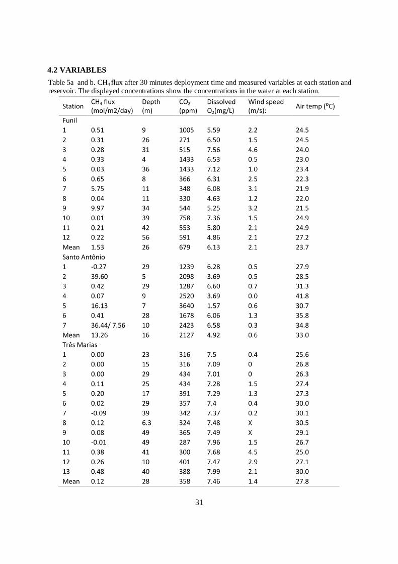
31

4.2 VARIABLES

Station CH4 flux (mol/m2/day)

Depth (m)

CO2 (ppm)

Dissolved O2(mg/L)

Wind speed (m/s):

Air temp (⁰C)

Funil

1 0.51 9 1005 5.59 2.2 24.5

2 0.31 26 271 6.50 1.5 24.5

3 0.28 31 515 7.56 4.6 24.0

4 0.33 4 1433 6.53 0.5 23.0

5 0.03 36 1433 7.12 1.0 23.4

6 0.65 8 366 6.31 2.5 22.3

7 5.75 11 348 6.08 3.1 21.9

8 0.04 11 330 4.63 1.2 22.0

9 9.97 34 544 5.25 3.2 21.5

10 0.01 39 758 7.36 1.5 24.9

11 0.21 42 553 5.80 2.1 24.9

12 0.22 56 591 4.86 2.1 27.2

Mean 1.53 26 679 6.13 2.1 23.7

Santo Antônio

1 -0.27 29 1239 6.28 0.5 27.9

2 39.60 5 2098 3.69 0.5 28.5

3 0.42 29 1287 6.60 0.7 31.3

4 0.07 9 2520 3.69 0.0 41.8

5 16.13 7 3640 1.57 0.6 30.7

6 0.41 28 1678 6.06 1.3 35.8

7 36.44/ 7.56 10 2423 6.58 0.3 34.8

Mean 13.26 16 2127 4.92 0.6 33.0

Três Marias

1 0.00 23 316 7.5 0.4 25.6

2 0.00 15 316 7.09 0 26.8

3 0.00 29 434 7.01 0 26.3

4 0.11 25 434 7.28 1.5 27.4

5 0.20 17 391 7.29 1.3 27.3

6 0.02 29 357 7.4 0.4 30.0

7 -0.09 39 342 7.37 0.2 30.1

8 0.12 6.3 324 7.48 X 30.5

9 0.08 49 365 7.49 X 29.1

10 -0.01 49 287 7.96 1.5 26.7

11 0.38 41 300 7.68 4.5 25.0

12 0.26 10 401 7.47 2.9 27.1

13 0.48 40 388 7.99 2.1 30.0

Mean 0.12 28 358 7.46 1.4 27.8

Table 5a and b. CH4 flux after 30 minutes deployment time and measured variables at each station and reservoir. The displayed concentrations show the concentrations in the water at each station.

32

Station Watertemp (⁰C)

pH Chl‒ A (μg/L)

Tot N (μg/L)

Tot P (μg/L)

Turbidity (NTU)

DOC (mg C/L)

Funil

1 27.64 7.61 3.40 1301 26 4.7 4.96

2 27.20 8.75 1.25 1767 24 8.2 3.88

3 26.71 9.36 4.30 1988 117 17.8 4.61

4 27.32 8.12 2.90 1759 45 6.5 4.18

5 26.85 9.30 1.20 1465 23 9.0 4.07

6 22.39 7.49 1.15 1973 88 56.0 6.36

7 22.29 7.33 X X X X X

8 26.44 7.31 X X 248 36.2 5.31

9 26.66 7.29 28.6 4033 170 34.0 5.57

10 27.42 9.23 2.80 1745 26 26.9 5.09

11 26.00 8.33 1.90 1474 35 11.3 4.41

12 22.18 7.68 0.90 1514 35 0.0 4.36

Mean 25.76 8.15 4.84 1902 76 19.0 4.80

Santo Antônio

1 27.63 6.47 1.28 1014 670 567.0 5.66

2 28.80 5.90 2.52 1167 34 5.0 10.99

3 27.73 5.92 1.48 1253 463 596.0 7.80

4 28.42 5.68 2.57 817 37 18.9 6.14

5 29.37 5.92 0.54 1133 28 8.1 8.11

6 27.60 6.83 2.64 1122 528 583.0 6.68

7 26.47 5.30 1.58 1037 46 20.4 6.07

Mean 28.00 6.00 1.80 1078 258 257.0 7.35

Três Marias

1 28.25 7.60 4.00 536 26 8.0 3.78

2 28.54 7.34 2.85 1048 27 24.6 3.79

3 27.41 7.26 3.85 490 22 6.9 3.52

4 28.43 7.25 2.30 541 26 6.6 3.56

5 28.31 7.51 2.35 650 35 2.5 3.61

6 29.80 7.63 0.55 771 23 1.7 3.66

7 30.40 7.94 2.85 772 20 2.4 4.54

8 29.50 7.76 1.80 732 19 12.4 4.13

9 29.33 7.86 3.70 749 20 2.2 3.75

10 28.07 7.85 2.40 399 17 2.3 11.69

11 28.02 8.07 0.80 361 40 5.5 3.55

12 28.07 7.57 0.65 435 12 1.1 3.77

13 28.50 8.22 3.80 698 20 2.6 3.50

Mean 28.66 7.68 2.45 629 24 6.0 4.37

33

4.2.1 Principial component analysis

A principial component analysis (PCA) was constructed where the following variables were

used as input variables:

CH4 concentration (ppm) Wind speed (m/s) Tot N (µg/L)

CH4 flux (mmol/m2/day) Water temperature (⁰C) Turbidity (NTU)

Dissolved O2 (mg/L) Air temperature (⁰C) DOC (µg/L)

O2 saturation (%) pH Chlorophyll‒a (µg/L)

Depth (m) Tot P (µg/L) CO2 (ppm)

The CH4 concentration is the concentration in each sample from the chambers. The dissolved

O2, CO2 and DOC are the concentrations in the water.

The variables CH4 flux, CH4 concentration, CO2 and DOC were related in the PCA of the

whole dataset. A relationship was also visible between dissolved O2, O2 saturation, pH and

depth. CH4, DOC and CO2 were located far away from O2, pH and depth. 50 % of the

variation in the dataset was explained in the PCA by component 1 and 2.

Figure 15 PCA of the whole data set with 15 variables.

34

The CH4 flux in Funil was related to the wind speed. A relationship was also visible between

dissolved O2, O2 saturation, pH, CO2 concentration and water temperature. This cluster and

the CH4 flux and wind speed were located in opposite quadrants which indicate a negative

relationship between them. 56 % of the variation in the dataset was explained in the PCA by

components 1 and 2.

A relationship between CH4 flux, CH4 concentration and DOC was visible in Santo Antônio.

The dissolved O2, O2 saturation, depth, pH, total P and turbidity were also related. These two

clusters were located far away from each other. 72 % of the variation in the dataset was

explained in the PCA by components 1 and 2.

Figure 17 PCA of Santo Antônio with 15 variables.

Figure 16 PCA of Funil with 15 variables.

35

In Três Marias the CH4 flux is related to the dissolved O2 saturation. A relationship was seen

between water and air temperature. 54 % of the variation in the dataset was explained in the

PCA by components 1 and 2.

Figure 18 PCA of Três Marias with 15 variables.

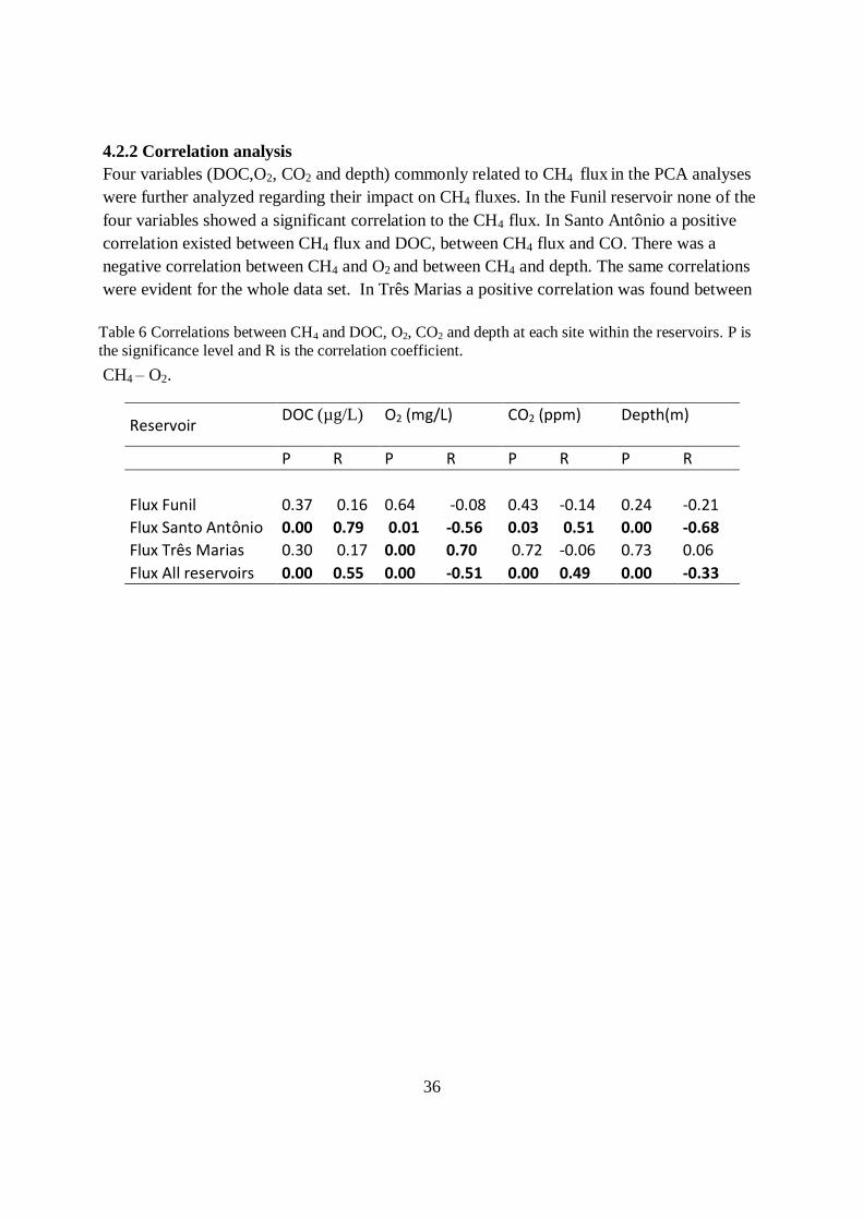
36

4.2.2 Correlation analysis

Four variables (DOC,O2, CO2 and depth) commonly related to CH4 flux in the PCA analyses

were further analyzed regarding their impact on CH4 fluxes. In the Funil reservoir none of the

four variables showed a significant correlation to the CH4 flux. In Santo Antônio a positive

correlation existed between CH4 flux and DOC, between CH4 flux and CO. There was a

negative correlation between CH4 and O2 and between CH4 and depth. The same correlations

were evident for the whole data set. In Três Marias a positive correlation was found between

CH4 ‒ O2.

Reservoir DOC (µg/L)

O2 (mg/L)

CO2 (ppm)

Depth(m)

P R P R P R P R

Flux Funil 0.37 0.16 0.64 -0.08 0.43 -0.14 0.24 -0.21

Flux Santo Antônio 0.00 0.79 0.01 -0.56 0.03 0.51 0.00 -0.68

Flux Três Marias 0.30 0.17 0.00 0.70 0.72 -0.06 0.73 0.06

Flux All reservoirs 0.00 0.55 0.00 -0.51 0.00 0.49 0.00 -0.33

Table 6 Correlations between CH4 and DOC, O2, CO2 and depth at each site within the reservoirs. P is

the significance level and R is the correlation coefficient.

thesignificance and R the correlation coefficient.

37

5 DISCUSSION

5.1 FUNIL RESERVOIR.

The 12 stations in Funil reservoir showed CH4 fluxes within the range of -0.04 and 13.15

mmol/m2/day. The mean flux was 0.99 mmol/m

2/day (Table 3). Most of the fluxes were

within a range of 0‒1 mmol/m2/day and three fluxes were above this range, located at stations

7 and 9 (Table 5a, appendix C).

By considering the water color, together with previous knowledge about the water quality in

Funil, it can be assumed that a great load of nutrients is transported into this reservoir. Funil

had the highest mean concentrations regarding chlorophyll‒a and total N, and the second

highest mean regarding the concentration of total P and DOC (Table 5b). The primary

production increases when nutrients like dissolved organic carbon, phosphorus and nitrogen

are available, which brings more organic material to the reservoir and the sediment. When

nutrients are available, a large CH4 production in the sediment could be assumed. The range

of CH4 fluxes in Funil is slightly higher than the range in Três Marias, but lower than earlier

results (Hamilton et al. 1995; Batlett et al. 1993; Galy‒Lacaux et al. 1997) . The oxygen level in

Funil enables methanotrophic bacteria to perform oxidation which is the process that probably

keeps down the CH4 emission level in Funil.

The initial water samples at all stations showed a higher concentration of CH4 compared to

the initial air sample. This is an expected result due to the oversaturation of CH4 in the water

that normally occurs in freshwater lakes (Jones & Mulholland 1998). At stations 1, 4, 6 and 7

the concentration of CH4 in the initial water sample was the highest. At these stations a

slightly higher flux of CH4 was present compared to the other stations (Figure 11).

Stations 7 and 9 had higher fluxes than the rest of the stations in Funil. Station 7 was located

in the riverine zone of the reservoir, where a higher water flux was present. To avoid drifting

too much, the boat used for the measurement was tied to a concrete block while the

measurements were performed. Earlier studies have shown a higher diffusive flux rate when

the chamber does not drift along with the water (UNESCO/IHA 2009). This could be a reason

for the high flux at this station. Because of the attachment, artificial turbulence might have

been created, leading to an increased CH4 emission rate. The high flux of CH4 in all three

chambers strengthens this theory and discourages the assumption that an ebullition bubble

caused the high flux. Thus, the results from this station cannot be considered to reflect a

natural flux. The initial water sample at station 7 had a high concentration of CH4. This shows

that great amounts of CH4 are available which makes the high flux at this station reliable, and

also dismiss the theory of an ebullition bubble.

38

Station 9 had a very high flux of CH4 in one of the chambers. This might be a result of an

ebullition bubble. This station had the highest levels of phosphorus, chlorophyll‒a and total N

within the reservoir, which probates the creation of CH4 (Table 5b). The oxygen level in the

water does not affect ebullition bubbles, since they ascend fast and thereby avoid oxidation.

Another evidence that reinforce the high flux to be an ebullition bubble is the low flux of CH4

in the other two chambers and low concentration of CH4 in the water (Figure 11). Earlier

results from 13 Swedish lakes, 11 North American lakes and literature values from 49 lakes

have shown that less than 10% of chamber measurements generally consist of ebullition

bubbles (Bastviken et al. 2004). In Funil one chamber at station 9 contains a probable

ebullition bubble. The rate in Funil was thereby 3%.

5.2 SANTO ANTÔNIO RESERVOIR

The CH4 fluxes in Santo Antônio ranged between -0.33 mmol/m2/day and 72.21 mmol/m

2/day

and the mean CH4 flux was 9.30 mmol/m2/day. The variance was 312,5 mmol/m

2/day which

indicates that there is a great variability in the data within the reservoir (Table 3, appendix C).

Very high fluxes of CH4 were observed at stations 2, 5 and 7 and lower fluxes at the other

four stations (Table 2). These three stations are situated in the flooded tributaries Jatuarana

(station 5) and Jaci‒Paraná (station 7) and the smaller Ceará Creek (station 2). Both Ceará and

Jatuarana have black water, caused by the high amount of organic material that is transported

into the tributary both from the catchment area and the flooded surrounding vegetation

(Castillo et al. 2004). Stations 2 and 5 were located in the middle of the flooded tributaries

where trees and other vegetation overtopped the water surface since no deforestation had

occurred before the flooding. This vegetation could especially be seen at station 5, where the

measurement station was surrounded by flooded palm trees. Flooded trees and other

vegetation were not visible to the same extent at station 2, but at this station gas bubble were

observed at the water surface. These bubbles were probably a result of ebullition. This station

was chosen by recommendations from people working with the environmental monitoring in

the area because of the high amount of bubbles and the black water characteristics. Before the

flooding this area was a Vareza but since the construction of the reservoir it has turned into a

bay. The chambers were placed straight above the bubbles when the measurements were

made. The depths at these two stations were shallow (5 and 7 meters) and the amount of

oxygen was the lowest within the reservoir (3.69 mg/l and 1.57 mg/l). These features, together

with the concentration of dissolved organic carbon (DOC 10.99 mg C/L and 8.11 mg C/L)

were factors that contributed to the high level of CH4 emissions at these two stations (Table

5a and 5b). Station 7 was located in the tributary Jaci‒Paraná next to and above macrophytes.

The water color in Jaci‒Paraná is somewhere between black and beige which indicates a

lower organic carbon content than in the earlier mentioned tributaries (Castillo et al. 2004). At

this location one chamber was placed above macrophytes and one control chamber was placed

in the water next to the macrophytes. The chamber placed on top of the macrophytes showed

39

a much higher flux of CH4 compared to the control chamber in the water (Figure 14, Table 2).

The control chamber had high CH4 flux, but not as high as at stations 2 and 5. The depth (10

m) and the oxygen level (6.58 mg/l) at this station was greater than at station 2 and 5 and the

DOC (6.07 mg C/L) was lower. This contributes to the explanation why the control chamber

had lower fluxes than these stations (Table 5a, 5b and 6). The reason why the chamber on top

of the macrophytes had a higher flux is that CH4 is transported from the sediments straight to

the atmosphere through the stems of the plants. If the transportation would have occurred in

the water column instead, the CH4 would partly have been oxidized into CO2 due to the

oxygen in the water. The control chamber had a lower CH4 flux due to this oxidation process.

In total, four stations were located in the tributaries, but the fourth station showed lower CH4

concentrations than the other three (station 4). This station was also situated in a flooded part

of the tributary Jaci‒Paraná, but in this area deforestation had occurred before the flooding.

Because of the deforestation, less organic material was available for decomposition. This

could be the reason why less CH4 were produced, even though the depth (9 m) and oxygen

level (3.69 mg/l) was low. The DOC concentration in the water was 6.14 mg C/l which is

lower than at stations 2 and 5 which further strengthens the reasoning.

In addition from the four stations located in the tributaries, three stations in the riverine zone

of the reservoir were used for measurements. None of these stations showed a flux of CH4

comparable to the fluxes in the tributaries, which probably is a consequence of the high speed

of the water, high oxygen level and great depth in this part of the reservoir (Table 5a). The

riverine zone has white water which carries large amounts of nutrients, like phosphorus. The

white water has a low Secchi depth which, together with the water speed, limits the primary

production. Thereby small amounts of organic material reach the sediment resulting in a

restricted methanogenesis activity. The high level of phosphorus and the low level of

chlorophyll‒a at the riverine stations (station 1, station 3 and station 6) in Santo Antônio

further support the explanation of the low CH4 flux (Table 5b). Station 6 was located close to

the dam and the boat was anchored to avoid drifting at this location. The CH4 flux at this

station was slightly higher than the flux at the other stations in the river (Table 5a). The initial

samples showed a generally higher concentration of CH4 in the water at the station with a

high flux rate. Station 4 had a comparably high concentration of CH4 in the water, but a low

flux (Figure 11).

Initial measurements taken from the air and the water downstream the reservoir at stations 8

and 9 showed a much higher concentration of CH4 in the air samples compared to the water

samples. This might be a result of the degassing that occurs in the outlet of the dam, when

CH4 is released to the atmosphere due to the turbulence in the turbines and the outlet. This

cause a higher concentration of CH4 in the air downstream the reservoir, compared to the air

upstream. The influence of degassing can occur 10 m to 50 km downstream the dam

(UNESCO/IHA 2009). Station 9 was located furthest away from the dam at a distance of 40

km. Station 10 downstream showed a different result in the initial samples of air and water.

40

The location of this station was a small flooded bay which was not influenced by the dam and

the river to the same extent as stations 8 and 9.

5.3 TRÊS MARIAS RESERVOIR

The results obtained in Três Marias showed a CH4 flux within the range of -0.31

mmol/m2/day and 0.56 mmol/m

2/day The mean CH4 flux was 0.12 mmol/m

2/day and the

variation is 0.04 mmol/m2/day (Table 3). The fluxes in Três Marias were significantly lower

than the fluxes in Funil and Santo Antônio (Table 4) and the variance within the reservoir was

very low. The concentration of CH4 in the initial water samples was lower at all stations

compared to Funil and Santo Antônio and this indicates that a small amount of CH4 is

available to generate diffusive emissions to the atmosphere. None of the chambers in Três

Marias showed an extraordinary result pointing at any occurrence of ebullition bubbles. Even

though the fluxes were within a narrow range, a relation could be seen between the initial

concentration of CH4 in the water and the CH4 fluxes. Stations 5, 8, 11, 12 and 13 had the

highest CH4 fluxes and these stations also had the highest concentrations of CH4 in the water

compared to the other stations. The chambers at station 5 were surrounded by macrophytes,

which might explain the relatively higher flux. The measurements at stations 1 and 2 were

done after a long heavy rain. Normally these kinds of weather conditions increase the amount

of CH4 that is emitted (Guerin et al. 2007), but the result did not show the highest flux of CH4

at these stations. The CH4 fluxes at all stations were very low, compared to Funil, Santo

Antônio and earlier studies (Hamilton et al. 1995; Batlett et al. 1993; Galy‒Lacaux et al. 1997),

even though some of the stations emitted more CH4 than the others. This low flux is probably

a result of a low organic carbon inflow in combination with a water body with a high level of

oxygen.

Temporal measurements were made in Três Marias during a 36 hours deployment time where

two chambers were placed next to the shore. These measurements where done in order to

investigate whether the increasing flux in the chambers followed a linear or exponential

pattern. The first chamber was placed in the water in the evening and the second chamber was

placed next to the first chamber in the morning, 15 hours later. The results from these

measurements (Figure 13) did not show any clear pattern, except from an increase in flux of

CH4 through time. The first chamber showed a linear increase (R2=0.94) in the flux during the

deployment time. Samples were taken every 30 minutes in the beginning of the deployment

time of the first chamber, but after 2 hours a heavy rain disturbed the measuring process. The

sampling stopped and continued when the deployment time had reached 15 hours. Thereby no

samples were made between the 2nd

and 15th

hour of deployment time in the first chamber.

The second chamber showed more of an exponential curve in the beginning of the

deployment time, followed by a decrease in flux with a small peak after about 26 hours. The

structure of the flux curve from the second chamber was more uneven than the curve from the

first chamber. These results indicate that equilibrium had not been established inside any of

41

the two chambers, which probably is a result of a too short deployment time and also because

of external disturbance. It is also difficult to conclude whether an increased flux in general

follows a linear or exponential pattern from these results, since the flux from each chamber

differed a lot. To be able to make better conclusions further temporal measurements need to

be done over a longer time period with more than one chamber at each measuring event. A

control chamber that was measured and repositioned every hour would be a good complement

to the other chambers.

5.4 COMPARISION OF CH4 EMISSIONS

The Wilcoxon Rank Sum Test (significance level 0.05) showed a significant difference in

CH4 flux between Funil and Três Marias (p < 0.05) and also between Três Marias and Santo

Antonio (p <0.05). The fluxes in Santo Antônio and Funil were not significantly different (p >

0.05) (Table 4). Both Funil and Três Marias had mean fluxes close to each other which also

were lower than the fluxes in Santo Antônio. This indicates that there is a similarity between

Funil and Três Marias. But the Wilcoxon Rank Sum test compares the variation between data

sets rather than similarities. Both Santo Antônio and Funil had outliers that cause a variation

in the flux. Funil had one station (station 9) and Santo Antônio 3 stations (2,5 and 7) with

probable ebullition bubbles, while Três Marias had no chamber with an outlying flux. The

cause of this might be that ebullition bubbles are produced in the sediment in Funil and Santo

Antônio, but not in Três Marias because a higher amount of organic material is available in

Funil and Santo Antônio.

The CH4 fluxes within the reservoirs were significantly different in Três Marias (p < 0.05)

and Funil (p < 0.05). The CH4 fluxes within Santo Antônio (p < 0.05) were not significantly

different, according to the same test (Table 4). Wilcoxon test evaluates if the variation among

the fluxes are similar and the overall variation does not say anything about that. This is why

the fluxes in Santo Antônio were not significantly different, even though the variation among

the data was the highest.

5.5 PRINCIPAL COMPONENT ANALYSIS (PCA)

Four Principal component analyzes were done; one for the whole dataset from all three

reservoirs and one for each reservoir.

In the PCA analysis for the whole dataset (Figure 15), the variables CH4 flux, CH4

concentration, DOC and CO2 were related. This relationship is probably based on the

methanogenesis and the respiration processes, where organic material is consumed and CH4

and CO2 are produced. Thus, a high concentration of DOC gives a high concentration of CH4

and CO2. The concentration of dissolved O2, O2 saturation, pH and depth were also related.

The CH4, DOC and CO2 are located in opposite direction from O2, pH and depth which means

42

that these clusters of variables affect the ecosystem in the reservoirs in different directions.

This indicates that a high emission rate of CH4 occurs when the oxygen level is low and when

there is a shallow depth.

The PCA of Funil (Figure 16) showed a positive relationship between CH4 flux and wind

speed. A relationship was also visible between the dissolved O2, O2 saturation, pH and CO2

concentration. The relationship between CH4 and wind speed was probably caused by an

increase in exposure area of the water towards the atmosphere due to the wind generated

waves, leading to an increased flux. The placement of CH4 in the opposite quadrant to the

cluster indicates that they affect the system in different directions. Since CO2 is related to O2 it

can be assumed that this relationship is caused by the oxidation process. The concentration of

CO2 in the water is high when there is a high oxidation rate, since CO2 is produced in this

process. A high oxidation rate occurs when the O2 level is high.

The PCA of Santo Antônio (Figure 17) showed a very different result compared to Funil.

There was a relation between the CH4 flux, CH4 concentration and DOC. The production of

CH4 relies on organic carbon, and the DOC is related to the available concentration of organic

carbon in the sediment, which explains this relationship. CH4 and DOC were located far away

from a cluster with the variables dissolved O2, O2 saturation, depth, total P and turbidity. Low

O2 concentrations, low depth and low turbidity are evident at the stations in the tributaries

where the CH4 fluxes are high, while the fluxes in the riverine zone are low together with a

high O2 concentration, depth and turbidity. The reason why total P is a part of this cluster is

that a lot of phosphorus is transported in the riverine zone. The explanation degree in

component 1 and 2 was 72 % and this degree of explanation was the highest among the PCA

plots.

The PCA performed in Três Marias (Figure 19) showed a relationship between CH4 flux and

dissolved O2. This relationship implies that a high O2 concentration gives a high CH4 flux, but

this is not how the reality works, since a high level of O2 benefits CH4 oxidation. This

relationship is probably a consequence of the low range in flux within the reservoir, caused by

chance. No other relationships were visible.

When comparing the four PCA:s, it can be seen that the results differed regarding the related

variables. The great variation is a result of three ecosystems with similar attributes, but also

different variables that affect the CH4 emissions to different extents. Another reason could be

the small amount of available data from each reservoir in combination with the high

variability among the data. Measurements were done during a limited time resulting in a low

amount of data with a high variability. If measurements were done during a longer period of

time with a wider spatial distribution, a more representative picture about the variables would

be obtained. Since the first PCA contains the whole dataset and thereby the highest amount of

data, this PCA should be the most representative one regarding the connections between the

variables.

43

5.6 EXPLAINING VARIABLES

According to the PCA:s, Table 5a, 5b and 6, the variables CO2, DOC, depth and O2 had the

strongest relationships to the CH4 fluxes.

Depth

There was a negative correlation between the CH4 concentration and the depth at the sampling

locations in Santo Antônio and among the three reservoirs together (Table 6). An explanation

for this relationship can be found in the hydrostatical pressure. When the water depth is small

the hydrostatical pressure is low. It is thereby easier for produced CH4 to overcome this

pressure and escape toward the atmosphere at shallow depths than in deeper areas. The

pathway of these emissions is through ebullition (Bastviken 2009). No correlation was seen in

Funil and Três Marias, probably due to the greather depths in these reservoirs compared to

Santo Antônio.

Concentration of CO2 in the water

There was a positive correlation between the CH4 flux and CO2 concentration in Santo

Antônio and among the three reservoirs together (Table 6).The highest CO2 concentration in

the water existed in the tributaries in Santo Antônio where the CH4 fluxes also were the

highest, especially station 2, 5 and 7 (Table 5a). Because of the high amount of available

organic carbon at these stations, both the production of CO2 and CH4 are favored, since CO2

and CH4 production rely on organic carbon. The main process that releases CO2 is the

respiration, and this process consumes O2. The O2 levels at these stations are generally low

and this indicates that respiration is the process that releases the CO2. There was no

significant correlation between the CO2 concentration and CH4 flux in Funil and Três Marias,

but it can be seen that the mean CO2 concentration was higher in Funil than in Três Marias

(Table 5a). The greater concentration of CO2 in Funil could be a product of a higher rate of

CH4 oxidation which further indicates that the production rate of CH4 is higher in Funil than

in Três Marias (Bastviken 2009). The higher concentration of CO2 in Funil can also be caused

by a higher respiration rate in Funil compared to Três Marias. The major reason why the

concentration of CO2 differed within and between the reservoirs is probably differences in

available organic matter and oxidation.

Dissolved O2

A negative correlation was observed between the dissolved O2 and the CH4 flux in Santo

Antônio and among the three reservoirs (Table 6). The dissolved oxygen concentration in

Santo Antonio was high in the main river and low in the tributaries at stations 2 and 5. The

high flux of CH4 at stations 2 and 5 can be explained by the low concentrations of dissolved

oxygen causing a limited oxidation of CH4. At station 7 the concentration of both CH4 and

oxygen was high, but the reason for the high CH4 flux was the macrophytes present at this

44

station. No negative correlation was observed in Funil and Três Marias, but a positive

correlation was observed between CH4 and O2 in Três Marias. This correlation was probably a

result of a very low CH4 flux which by chance was correlated with O2. Três Marias had the

highest O2 concentration in the water which partly could be an explanation why the flux of

CH4 was low in this reservoir. Funil reservoir had a lower mean concentration of O2 but still

enough for oxidation to be performed (Soares et al. 2008). The oxidation rate might be greater

in Três Marias than in Funil due to the difference in dissolved O2.This could be the reason for

the higher flux of CH4 in Funil. The level where the concentration of O2 is considered to

cause a hypoxic environment is at a concentration of 2‒3 mg/l (Kalff 2002) and there was

only one station (station 5 in Santo Antônio) who had an oxygen level below this

concentration.

Dissolved organic carbon, DOC

There was a positive correlation between CH4 and DOC in Santo Antônio and among the

three reservoirs together (Table 6). The highest concentration of dissolved organic carbon was

found in Santo Antônio at stations 2 and 5 which also had high fluxes of CH4. Since organic

material is required for the methanogenesis process locations with high organic carbon

content in the sediment produce the largest amount of methane. A high concentration of

dissolved organic carbon in the water is related to the carbon content in the sediment. No

correlations were seen in Funil and Três Marias.

Other measured variables

No clear pattern between CH4 flux and the variables wind speed, temperature, pH, turbidity,

total N, total P and chlorophyll‒a was observed. One reason why no relationship between

wind speed and the CH4 fluxes was visible is that there is no major difference in wind

between the stations and reservoirs. The wind does not directly affect the diffusive emissions

since the emissions are controlled by the aquatic boundary layer (McGillis et al. 2001), but

the aquatic boundary layer is affected by the wind. If greater differences were evident in wind

speed a higher CH4 flux would be expected at locations with low wind speed (Sharpe et al.

2002). No clear pattern was seen between the air and water temperature and the flux of CH4 in

any of the reservoirs. Earlier results have suggested that the temperature affects the CH4

emissions because the methanogenesis process rate increases with temperature (Conrad 2002).

Since the measurements were done at one occasion in every reservoir the connections

between temperature and CH4 emissions could not be observed. If measurements would have

continued during the year the effect of this variable on the CH4 emissions would probably be

different. The turbidity in not related to the CH4 emissions in general in the study, but the

turbidity in Santo Antônio was high where the fluxes were low. This variable would probably

have a stronger connection to CH4 emissions in a larger study, where a high turbidity would

exist at locations with a low flux. The total N concentration, total P concentration and

45

Chlorophyll‒a did not have a clear connection to the CH4 emissions, but these variables are

influencing the amount of organic carbon within a reservoir. In the long run these variables

are important in the processes related to CH4, but this could not be shown in this study.

Age of reservoir

Another factor that affects the CH4 flux is the age of the reservoir. Santo Antônio is a newly

constructed reservoir and thereby large areas in the tributaries are flooded. When this

happens, newly constructed organic material is decomposed and turned into CH4. Funil

reservoir and Três Marias reservoir were constructed in 1960 and therefore no easily

decomposed organic material originated from the time of construction is left in this reservoir.

This could be another reason why the CH4 fluxes in Santo Antônio were so much higher than

the fluxes in Funil and Três Marias (Barros et al. 2011).

5.7 LINEAR AND NON‒LINEAR CALCULATIONS OF FLUX

The calculations of the CH4 flux can be done in two different ways; with a linear

approximation and with a non‒linear function (Figure 12). When the increasing flux in a

chamber follows a pattern that has more of an exponential character than linear, the non‒

linear function gives a better result. This is why the greatest differences in flux obtained from

the two methods were found where the fluxes are the highest. Since the non‒linear flux takes

into account the decrease in flux during time, the result from the non‒linear calculations can

be considered to reflect the reality in the chamber better than the linear approximation. The

results obtained from the different methods showed a higher flux when the non‒linear method

was used compared to the linear. These differences were visible at the stations with the

highest flux. The linear approximation does not follow the non‒linear function because the

high emissions are non‒linear, while lower fluxes have more of a linear behavior. The

temporal measurements in Três Marias (Figure 13) showed a linear pattern in the first

chamber and more of an exponential pattern in the second chamber. The fluxes in both

chambers were calculated by the non‒linear functions. It is difficult to decide whether the

increased flux of CH4 follows a linear or an exponential pattern in the chamber from these

results. Chamber 1 was placed in the water in the afternoon while chamber 2 was placed in

the water in the morning, and this difference in time might affect the CH4 fluxes because of

differences in light, temperature and the activity in the surrounding water. The chambers were

located next to each other, which means that they should be in touch with the same

concentration of CH4 in the water. The difference in CH4 flux in the two chambers is big and

there is no clear explanation to this.

46

5.8 EVALUATING THE METHOD

The floating chamber method has been used worldwide in many different constellations, both

for CO2 measurements and CH4 measurements. It is a very easy and cheap method to use and

the theory behind the method is easy to understand. There were many situations in the field

where the reliability regarding the method was discussed, due to the errors that can occur in

connection to the measurements. Also during the analysis with the GC many questions

appeared regarding the credibility in the results. The GC showed uneven results and the

standard curve differed a lot through the days of analyses. The method has been dismissed by

several researchers mainly because the floating chamber method is said to increase the

turbulence at the water surface which enables more CH4 to diffuse to the air (Raymond &

Cole 2001). By constructing chambers with wall that extends into the water, this turbulence

can be avoided (Matthews et al. 2003). The chambers also isolate the water surface from the

impact of wind. However, studies show that the exchange of gas is controlled by the

turbulence in the aquatic boundary layer and therefore the wind does not have a great

influence on the emissions (McGillis et al. 2001). Guerin et al. (2007) investigated this

method further and also compared it with the eddy covariance technique. The conclusion was

that the floating chamber method is a reliable method. The main thing to keep in mind, except

from the extended chamber walls, is to leave the chambers drifting while the measurements

are made. The results from the two stations where the boat was fixed are unreliable because of

this.

5.9 ERRORS

The errors that possibly occurred in the field and in the lab were mostly connected to the

chamber construction or the sampling method. The three chambers that were used were a bit

bigger than most used chambers, which might give a different flux. The UNESCO/IHA

measurement specification (UNESCO/IHA 2009) suggests a chamber with the volume 20 dm3

and an area of 0.2 m2 and the volume of the three chambers used in this study was 35.75 dm

3

and an area was 16.58 dm2 and 16.66 dm

2. No optimal extension of the chamber walls into the

water was considered; therefore the buoys were attached without any defined height above the

water surface. If the walls extend to far into the water, the turbulence in the boundary layer

might get affected.

Another possible error is the deployment time. There was a lack of certainty regarding the

optimal deployment time of the chambers, since there was no time to try out the best time

interval and length of measurements. The 3 x 10 minute time interval was decided from

previous studies and also because this timespan suited with the other groups who shared the

boat in the field. Because of this important moments regarding the CH4 flux behavior might

have been left out in the measurements. The obtained fluxes from the first 10 and 20 minutes

were not used in the results because of their insecurity. Also the limited numbers of

measurement taken at each reservoir could give rise to results that do not correspond to the

47

values that reflect the concentrations and fluxes in the whole reservoir. Another error was the

unequal hour of sampling during the day at all stations. The light and temperature differs

depending on the hour and this might affect the CH4 emissions. Therefore a comparison

between the CH4 fluxes might not be reliable since the fluxes represent different time span.

The GC gave rise to possible errors. The integrated area that was used to calculate the CH4

concentration could be integrated very differently depending on where the baseline was

drawn. This lead to an uncertain standard curve in many cases, and a big difference among the

constructed standard curves. If more time were available the samples could have been

analyzed by the GC more than one time, which would have given more secure results.

5.10 SUMMARY OF THE RESULTS

The CH4 fluxes in Funil Reservoir were within the range of -0.04 to 13.16

mmol/m2/day, and the emissions within the reservoir were significantly different.

The CH4 fluxes in Santo Antônio Reservoir were within the range of -0.33 to 72.21

mmol/m2/day, and the emissions within the reservoir were not significantly different.

The CH4 fluxes in Três Marias Reservoir were within the range of -0.31 to 0.56

mmol/m2/day, and the emissions within the reservoir were significantly different.

Santo Antônio and Três Marias had significantly different CH4 fluxes. So did Funil

and Três Marias. Funil and Santo Antônio had not significantly different CH4 fluxes.

The CH4 flux was positively correlated with CO2 and DOC and negatively correlated

with O2 and depth in Santo Antônio. The same correlations were evident for the whole

data set.

48

6 CONCLUSION The measured fluxes in the three reservoirs ranged from -0.33 to 72.21 mmol/m

2/day and the

mean flux was 2.31 mmol/m2/

day. These fluxes are low compared to earlier results. The

variation in CH4 flux within and between the reservoirs was significantly different in a major

part of the comparisons. Variables that increase the CH4 emission rate were illuminated, even

though most fluxes were significantly different. A low depth and low O2 concentration

increase the CH4 emission rate. A high concentration of DOC and CO2 indicates that a high

amount of organic carbon is available for the production of CH4, leading to an increased CH4

emission rate.

49

7 REFERENCES

Abril G, Guérin F, Richard S, Delmas R, Galy‒Lacaux C, Gosse P, Tremblay A, Varfalvy L,

Dos Santos M A, Matviento B. 2005. Carbon dioxide and methane emissions and the carbon

budget of a 10-year old tropical reservoir (Petit Saut, French Guiana). Global Biogeochemical

Cycles 19:16

Arantes F, Santos H B D, Rizzo E, Sato Y, Bazzoli N. 2011. Collapse of the reproductive

process of two migratory fish (Prochilodus argenteus and Prochilodus costatus) in the Três

Marias Reservoir, São Francisco River, Brazil. Journal of Applied Ichthyology 27:847‒853

Barros N, Cole J J, Tranvik L J, Prairie Y T, Bastviken D, Huszar V L M, Giorgio P, Roland

F. 2011. Carbon emission from hydroelectric reservoirs linked to reservoir age and latitude.

Nature Geoscience 4:593-596

Batlett K B & Harris R C. 1993. Review and Assessment of Methane Emission from

Wetlands. Chemosphere 26:261‒320

Bastviken D, Cole J, Pace M, Tranvik L. 2004.Methane emissions from lakes: Dependence of

lake characteristics, two regional assessments, and a global estimate. Global Biogeochemical

cycles. doi:10.1029/2004GB002238

Bastviken D. 2009. Methane. In: Likens G. (ed.). Encyclopedia of Inland Waters, pp. 783-805

Oxford, Elsevier Inc.

Braga B, Rocha O, Tundisi J.1998. Dams and the environment: the Brazilian experience.

International Journal of Water Resources Development 14:127-140

Branco C W C, Rocha M I A, Pinto G F S, Gômara G A, Filippo R D. 2002. Limnological

features of Funil Reservoir (R.J., Brasil) and indicator properties of rotifers and cladocerans

of the zooplankton community. Lakes & reservoirs: Research and Management 7:87‒92

Brito S L, Barbosa P M M, Coelho R M P.2011. Zooplankton as an indicator of trophic

conditions in two large reservoirs in Brazil. Lakes & Reservoirs: Research and Management

16:253–264

Carolsfeld J, Harvey B, Ross C, Baer A. 2003. Migratory fishes of South America: biology,

fisheries and conservation status. The International Bank of Reconstruction and Development

/ The World Bank, Washington

Carvalho N O, Ross J, Silva L F A, Café F A, Coimbra A R S, Lima J E F W, Celeri A, Alves

C F, Ide C N, Val L A A, Braga A. 2011. Evaluating of temporal variability of rainfall, water

discharge and sediment yield in large river basins of Brazil. In: Bilibio C, Hensel O, Selbach

J. Sustainable water management in the tropics and subtropics and case studies in brazil, pp.

149‒170. Jaguarão/RS: Fundacão Universidade Federal do Pampa,

UNIKASSEL;PGCultUFMA

50

Castillo M M, Allan J D, Sinsabaugh R L, Kling G. 2004. Seasonal and interannual variation

of bacterial production in lowland rivers of the Orinoco basin. Freshwater Biology 49:1400–

1414

Cimbleris A C P. Carbon budget in hydroelectric reservoirs of FURNAS centrais eléctrica

S.A., Brazil www‒document 2007‒05‒18 http://www.dsr.inpe.br/projetofurnas/index_e.html

collected 2012‒03‒21

Conrad R. 2002.Control of microbal methan production in wetland rice fields. Nutrient

Cycling in agroecosystem 64:59‒69

Fonseca R, Barriga F J A S, Theodoro S, Canário T. 2007. The Três Marias Reservoir: A sink

for sediments outcoming from over‒erosion of soils in Minas Gerais, Brazil. In: Gunkel G, do

Carmo Sobral M (eds). Reservoir and river basin Mangaement: Exchange of Experiences

from Brazil, Portugal and Germany, pp.182‒197. Universitätsverlag der TU Berlin. Berlin

Galy Lacaux C, Delmas R, Jambert C, Dumestre J F, Labroure L, Richard S, Gosse P.

1997. Gaseous Emissions and Oxygen Consumption in Hydroelectric Dams : A Case Study in

French Guyana. Global Biogeochemical Cycles 11:471‒483

Guyot J, Filizola N, Quintanilla J, Cortez J. 1996. Dissolved solids and suspended sediment

yields in the Rio Madeira basin, from the Bolivian Andes to the Amazon. Walling D E, Webb

B W (red.) Erosion and Sediment Yield: Global and Regional Perspectives, ss 55‒

63.Department of Geography, University of Exete, UK

Hamilton S K, Sippel S J, Melack J M. 1995.Oxygen Depletion and Carbon Dioxide and

Methane Production in Waters of the Pantanal Wetland of Brazil. Biochemistry 30:115‒141

IAEA. n. d. Brazil. www‒document http://www‒

pub.iaea.org/mtcd/publications/pdf/cnpp2003/cnpp_webpage/PDF/2000/Reports/BRAZIL.pdf

collected 2012‒04‒11

Jacobson M Z. 2005. Pressure, density, and composition. In: Jacobson MZ (ed.).

Fundamentals of atmospheric modelling, pp 16‒17. Cambridge University Press, New York.

Jones J B, Mulholland P J. 1998. Methane input and evasion in a hardwood

forest stream: Effects of subsurface flow from shallow and deep pathways.

Limnology and Oceanography 43:1243‒1250.

Jones J G, Simon B E M, Gardener S. 1982. Factors Affecting Methanogenesis and

Associated Anaerobic Processes in the Sediment of a Stratifyed Eutropic Lake. Journal of

General Microbiology 128:1‒11

51

Junk WJ, Piedade M T F, Schöngart J, Haft M C, Adeney J M, Wittmann F. 2011 A

Classification of Major Naturally‒Occurring Amazonian Lowland Wetlands. Wetlands

31:623‒640

Kalff J. 2002. Limnology: inland Water Ecosystem. Prentice‒Hall, Upper

Saddle River, New Jersey

Khan F A & Ansari A A. 2005. Eutrophication: An ecological Vision. The Botanical Review

71:449–482

Klapper H. 1998. Water quality problems in reservoirs of Rio de Janeiro, Minas Gerais and

São Paulo. International Reviews of Hydrobiology 83:93–10

Latrubesse E M, Stevaux T J C, Sinha R. 2005. Tropical rivers. Geomorphology 70:187‒

206

Leite N K, Krusche A V, Ballester M V R, Victoria R L, Richey J E, Gomes B M. 2010.

Intra and interannual variability in the Madeira River water chemistry and sediment load.

Biogeochemistry 1‒15

Louis V L, Kelly C A, Duchemin E, Russ J W M, Rosenberg D M. 2000. Reservoir surfaces

as sources of greenhouse gases to the atmosphere: a global estimate. BioScience 50:766‒775

Lyons W B, Bird D A.1995. Geochemistry of the Madeira River, Brazil—comparison of

seasonal weathering reactions using a mass‒balance approach. Journals of South America

Earth Sience 8:97–101

Mathworks. Principal Component Analysis (PCA) www‒document

http://www.mathworks.se/help/toolbox/stats/brkgqnt.html#f75476 collected 2012‒05‒18

Matthews C J D, Saint‒Louis V L, Hesslein R H. 2003. Comparison of three techniques used

to measure diffusive gas exchange from sheltered aquatic surfaces. Environmental Science

Technology 37:772–780.

McGillis, W R, Edson J B, Ware J D, Dacey J W H, Hare J H, Fairall C W, Wanninkhof

R.2001. Carbon dioxide flux techniques performed during GasEx‒98. Marine Chemistry

75:267–280

Naturskyddsföreningen. Klimat och energi‒fallstudie:Brasilien.

www‒document 2009‒07‒02 http://www.naturskyddsforeningen.se/natur‒och‒

miljo/klimat/energi/vattenkraft/fallstudier/brasilien/ collected 2012‒04‒11

Odebretcht. Businesses and interests‒ Energy. www‒document 2012‒05‒10

http://www.odebrecht.com/en/businesses‒and‒interests/energy collected 2012‒05‒13

52

Pircher W. 1993. 36 000 dams and still more needed. International Water

Power & Dam Construction 45:15–18.

Poole C F.2003. Instrumental aspects of gas chromatography. In: Poole CF (ed.). The Essence

of Chromatography, pp 171‒ 256. Elsevier science B.V, Netherlands

Raymond P A, Cole J J. 2001. Gas exchange in rivers and estuaries:

choosing a gas transfer velocity. Estuaries 24:312–317.

Roland F, Vidal L O, Pacheco F S, Barros N O, Assireu A, Ometto J P H B, Cimbleris A C P,

Cole J J. 2010. Variability of carbon dioxide flux from tropical (Cerrado) hydroelectric

reservoirs. Aquatic science 72:283‒293

Rosa L P, Santos M A, Matvienko B, Santos E O, Sikar E. 2004. Greenhouse Gas Emissions

from Hydroelectric Reservoirs in Tropical Regions. Climate Change 66:9‒21

Rosa L P, Santos M A, Matvienko B, Sikar E. 2002. Hydroelectric reservoirs and global

warming. RIO 02 World Climate & Energy Event 6‒11 January 2002.

Sampaio E V & López C M. 2003 Limnologias física, química e biológica da represa de Três

Marias e do São Francisco. In: Godinho HP & Godinho (ed). Aguas, Peixes e Pescadores do

São Francisco das Minas Gerais, pp. 71–92. Minas, Belo Horizonte.

SantoAntônio Energia. The constructions of the project. www‒document 2009

http://www.santoantonioenergia.com.br/site/portal_mesa/en/usina_santo_antonio/geracao_de_

energia/geracao_de_energia.aspx collected 2012‒05‒13

Santos M A, Rosa L P, Sikar B, Sikar E, Santos EO.2006. Gross greenhouse gas fluxes from

hydro‒power reservoir compared to thermo‒power plants. Energy Policy 34:481‒488

Sharpe R R, Harper L A, Byers F M. 2002. Methane emissions from swine lagoons in

Southeastern US. Agriculture, Ecosystems & Environment 90:17‒24

SLCF. Metan www‒document 2011‒03‒31 http://www.smhi.se/slcf/Om‒SLCF/metan‒

1.20073 collected 2012‒05‒18

Soares M C S, Marinho M M, Huszar V L M, Branco C W C, Azevedo S M F O. 2008. The

effect of water retention time and watershed features on the limnology of two tropical

reservoirs in Brazil. Lakes & Reservoirs: Research and Management 13:257‒269

Stallard R F, Edmond J M. 1983. Geochemistry of the Amazon 2. The influence of geology

and weathering environmenton the dissolved‒load. Journal of Geophysical Research

88:9671–9688

Switker B & Bonilha P. Muddy waters‒ Consequences of damming the Amazon principal

tributary. www‒document 2007‒06‒35 http://www.internationalrivers.org/en/latin‒

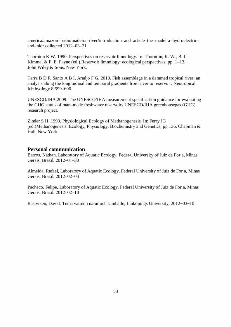
53

america/amazon‒basin/madeira‒river/introduction‒and‒article‒the‒madeira‒hydroelectric‒

and‒hidr collected 2012‒03‒21

Thornton K W. 1990. Perspectives on reservoir limnology. In: Thornton, K. W., B. L.

Kimmel & F. E. Payne (ed.).Reservoir limnology: ecological perspectives. pp. 1‒13.

John Wiley & Sons, New York.

Terra B D F, Santo A B I, Araújo F G. 2010. Fish assemblage in a dammed tropical river: an

analysis along the longitudinal and temporal gradients from river to reservoir. Neotropical

Ichthyology 8:599‒606

UNESCO/IHA.2009. The UNESCO/IHA measurement specification guidance for evaluating

the GHG status of man‒made freshwater reservoirs.UNESCO/IHA greenhousegas (GHG)

research project.

Zinder S H. 1993. Physiological Ecology of Methanogenesis. In: Ferry JG

(ed.)Methanogenesis: Ecology, Physiology, Biochemistry and Genetics, pp 136. Chapman &

Hall, New York.

Personal communication Barros, Nathan, Laboratory of Aquatic Ecology, Federal University of Juiz de For a, Minas

Gerais, Brazil. 2012‒01‒30

Almeida, Rafael, Laboratory of Aquatic Ecology, Federal University of Juiz de For a, Minas

Gerais, Brazil. 2012‒02‒04

Pacheco, Felipe, Laboratory of Aquatic Ecology, Federal University of Juiz de For a, Minas

Gerais, Brazil. 2012‒02‒10

Bastviken, David, Tema vatten i natur och samhälle, Linköpings University, 2012‒03‒10

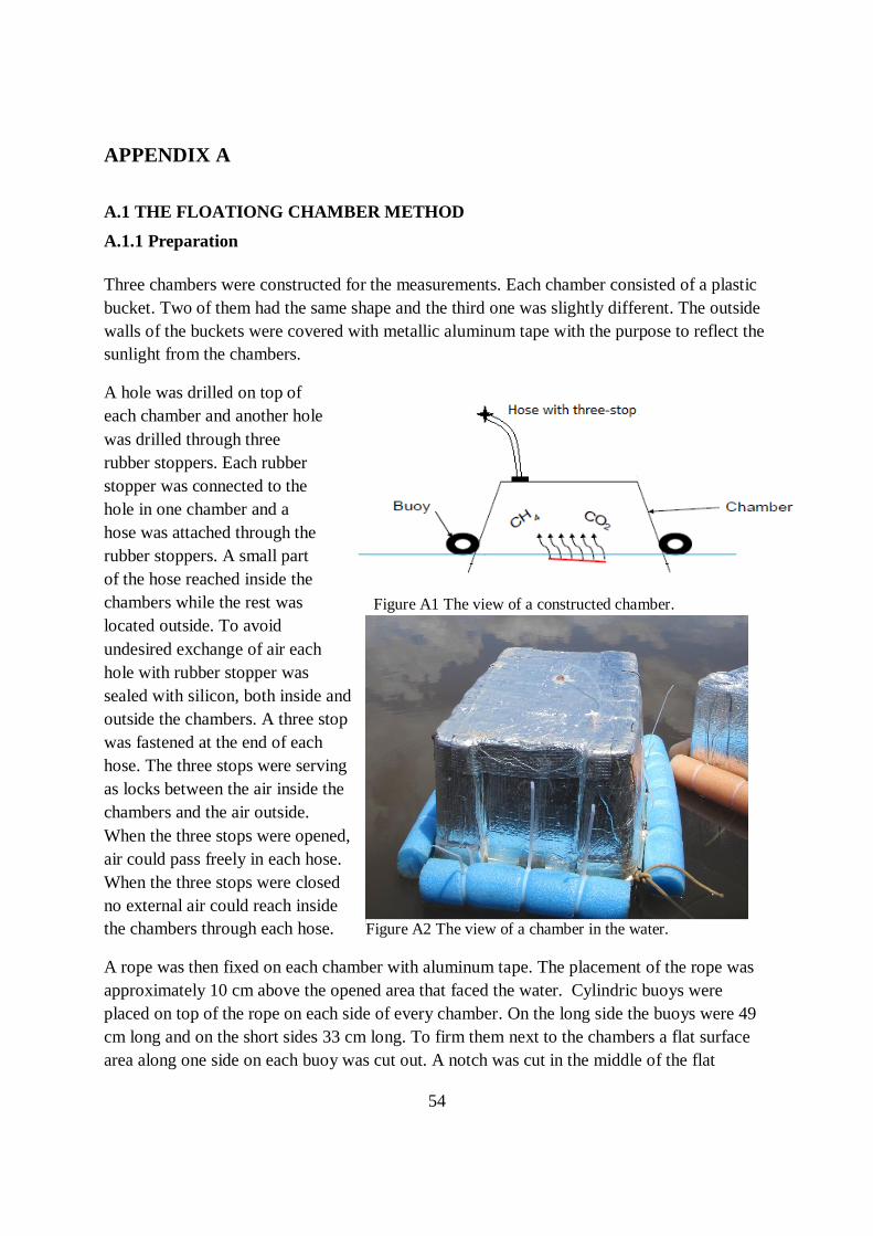
54

APPENDIX A

A.1 THE FLOATIONG CHAMBER METHOD

A.1.1 Preparation

Three chambers were constructed for the measurements. Each chamber consisted of a plastic

bucket. Two of them had the same shape and the third one was slightly different. The outside

walls of the buckets were covered with metallic aluminum tape with the purpose to reflect the

sunlight from the chambers.

A hole was drilled on top of

each chamber and another hole

was drilled through three

rubber stoppers. Each rubber

stopper was connected to the

hole in one chamber and a

hose was attached through the

rubber stoppers. A small part

of the hose reached inside the

chambers while the rest was

located outside. To avoid

undesired exchange of air each

hole with rubber stopper was

sealed with silicon, both inside and

outside the chambers. A three stop

was fastened at the end of each

hose. The three stops were serving

as locks between the air inside the

chambers and the air outside.

When the three stops were opened,

air could pass freely in each hose.

When the three stops were closed

no external air could reach inside

the chambers through each hose.

A rope was then fixed on each chamber with aluminum tape. The placement of the rope was

approximately 10 cm above the opened area that faced the water. Cylindric buoys were

placed on top of the rope on each side of every chamber. On the long side the buoys were 49

cm long and on the short sides 33 cm long. To firm them next to the chambers a flat surface

area along one side on each buoy was cut out. A notch was cut in the middle of the flat

Figure A1 The view of a constructed chamber.

Figure A2 The view of a chamber in the water.

55

surface to make them even more stable. This notch was attached on top of the rope on the

chambers. The buoys were tied to the rope by cable ties. The ends of each fixed rope were

tied together and ca 2 m of the rope was left with the purpose to fix each chamber to the boat

while making measurements. The buoys were blue, yellow and orange giving each chamber

one of these color.

The chambers were tested in a pond after the construction to make sure they were floating in a

stable way (Figure A2). The three stops attached to the hoses were opened when the chambers

were placed in the water. The purpose was to ease the process of stabilizing the pressure

within the chamber with the atmospheric pressure. The chambers were a bit unstable at the

start, but got stabilized after a short time in the water. To further regulate the buoyancy of the

chambers the buoys were moved up and down. The movements enabled the chambers to get

into a straight position in the water. The chambers were moved around while testing them to

make sure they resisted rain and waves and other weather conditions. The high placement

level of the buoys gave chamber‒walls that extended about 10 cm below the surface water

level. By having chamber‒walls underneath the water surface, influences caused by weather

conditions could be minimized (UNESCO/IHA 2009). When testing the chambers it could

clearly be visible that this way of placing the buoys made the chambers more stable. The

reason for choosing three chambers was that replicates were required to ensure more secure

results and also to enable ebullition bubbles to be captured.

To be able to calculate the flux of CH4, the volume of the chambers above the water surface

were measured and also the water‒facing area of the chambers. First the water level in

relation to the floating chambers needed to be established. This was done in the pond by

marking each chamber where the water level was located. The volume was measured by

turning the chambers upside down and then filling them with water to the marked level. Each

chamber had a volume of 35.75 liters. The water facing area was calculated by scales. The

area of the blue and yellow chamber was 16.58 dm2 and the area of the orange was 16.66 dm

2.

The vials that were used to store the samples were filled with a saturated salt solution before

the measurements were done. Water and salt were mixed until the salt was dissolved and the

solution was saturated. At 20⁰C the concentration of saturation is approximately 300 g

salt/liter water (UNESCO 2009). The vials were placed in the salt solution until they were

completely filled and a rubber stopper was used to enclose each vial. A small needle

connected to a syringe was attached through the rubber stopper before the enclosing process.

This enabled overspill water to escape through the needle and syringe which made the vial

close properly. Each vial was visually inspected to make sure that no bubbles occurred in the

vial. If no bubbles were visible the syringe with needle was pulled out from the rubber

stopper. The vial was sealed with a metal lid on top of the rubber stopper to make sure no

external air entered the vial. The 385 vials used for the study went through the same

procedure. It is important to make sure that no air bubbles occur in the vials straight after they

56

are closed with the rubber stopper because external air bubbles might affect the CH4 gas.

Bubbles might occur later due to differences in temperature or pressure compared to present

temperature and pressure when preparing the vials. Bubbles that occur later consist of vacuum

and will thus not affect the result of the measurements. The salt solution was replaced by the

air sample in the field. By using the salt solution no disturbing gas occurred in the vial when

the sample was transferred into it and thereby no other gas could affect the sampled gas.

A.1.2 In the field

The measurements were made with three chambers at every measurement station in each

reservoir and a boat was used to reach these stations. The chambers were placed in the water

next to each other with the three stops opened. The three stops were closed after a while when

the chambers were stabilized in the water. The time of this occurrence was written down in a

protocol. An initial air sample was collected with a 60 ml syringe with three stop straight

above the chambers. The three stop attached to the syringe was closed and the time of

sampling was written down in the protocol. Then an initial 60 ml water sample was collected

from the surface water next to the three chambers with a 60 ml syringe connected to a three

stop. 20 ml of water was then pressed out of the syringe and replaced by air and then the three

stop was closed. After this procedure the syringe contained 40 ml of water and 20 ml of air.

The time for the sampling was written down in the protocol and then the syringe was shaken

for 1 minute. Equilibrium was achieved between the gas in the gas phase and the gas in the

water phase by shaking the syringe. The gas phase was transferred to another syringe when 1

minute had passed (Figure A3). It was very important that no water went with the gas into the

new syringe.

Figure A3 The procedure of taking the initial water sample.

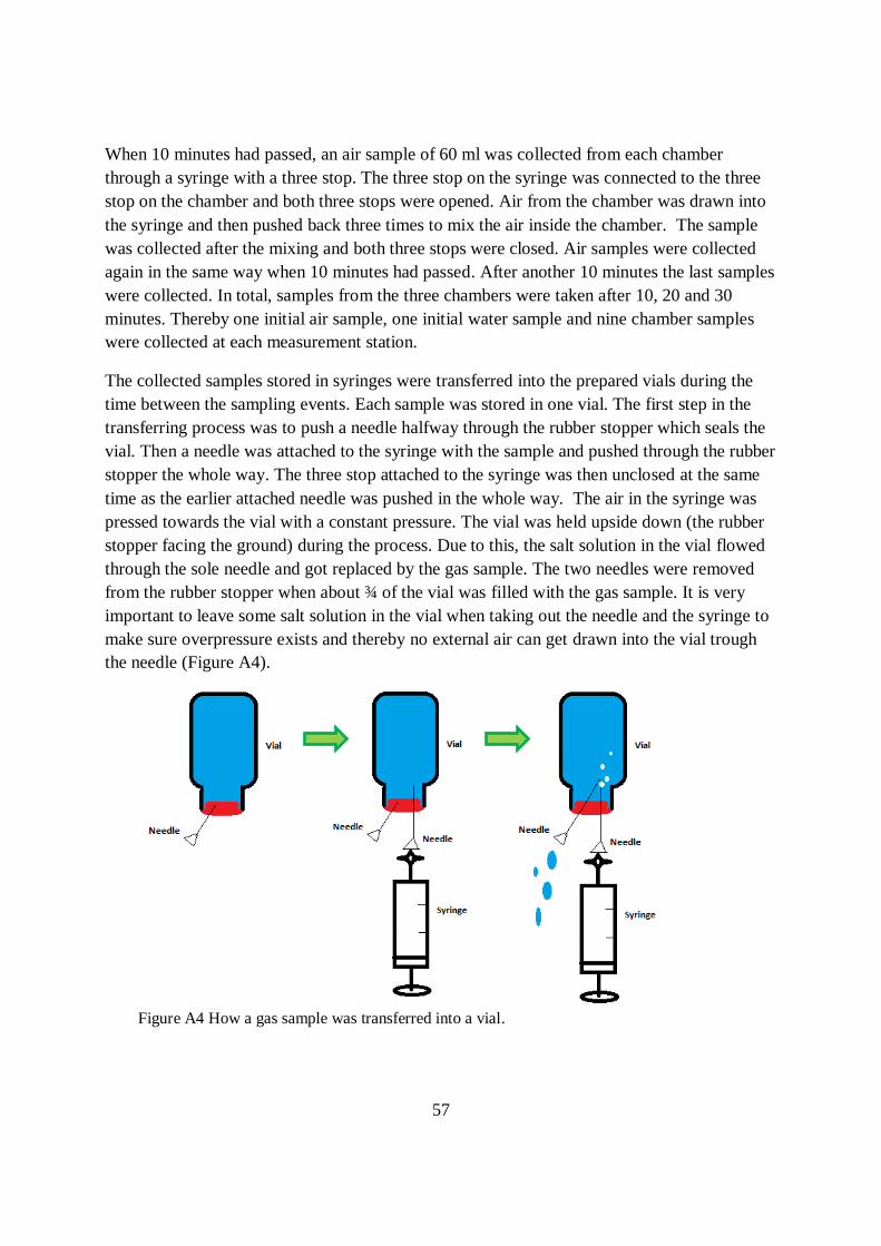
57

When 10 minutes had passed, an air sample of 60 ml was collected from each chamber

through a syringe with a three stop. The three stop on the syringe was connected to the three

stop on the chamber and both three stops were opened. Air from the chamber was drawn into

the syringe and then pushed back three times to mix the air inside the chamber. The sample

was collected after the mixing and both three stops were closed. Air samples were collected

again in the same way when 10 minutes had passed. After another 10 minutes the last samples

were collected. In total, samples from the three chambers were taken after 10, 20 and 30

minutes. Thereby one initial air sample, one initial water sample and nine chamber samples

were collected at each measurement station.

The collected samples stored in syringes were transferred into the prepared vials during the

time between the sampling events. Each sample was stored in one vial. The first step in the

transferring process was to push a needle halfway through the rubber stopper which seals the

vial. Then a needle was attached to the syringe with the sample and pushed through the rubber

stopper the whole way. The three stop attached to the syringe was then unclosed at the same

time as the earlier attached needle was pushed in the whole way. The air in the syringe was

pressed towards the vial with a constant pressure. The vial was held upside down (the rubber

stopper facing the ground) during the process. Due to this, the salt solution in the vial flowed

through the sole needle and got replaced by the gas sample. The two needles were removed

from the rubber stopper when about ¾ of the vial was filled with the gas sample. It is very

important to leave some salt solution in the vial when taking out the needle and the syringe to

make sure overpressure exists and thereby no external air can get drawn into the vial trough

the needle (Figure A4).

Figure A4 How a gas sample was transferred into a vial.

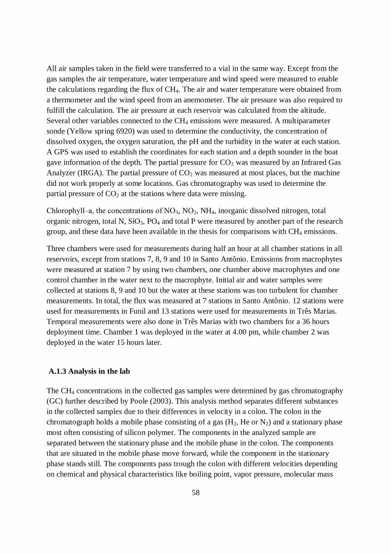
58

All air samples taken in the field were transferred to a vial in the same way. Except from the

gas samples the air temperature, water temperature and wind speed were measured to enable

the calculations regarding the flux of CH4. The air and water temperature were obtained from

a thermometer and the wind speed from an anemometer. The air pressure was also required to

fulfill the calculation. The air pressure at each reservoir was calculated from the altitude.

Several other variables connected to the CH4 emissions were measured. A multiparameter

sonde (Yellow spring 6920) was used to determine the conductivity, the concentration of

dissolved oxygen, the oxygen saturation, the pH and the turbidity in the water at each station.

A GPS was used to establish the coordinates for each station and a depth sounder in the boat

gave information of the depth. The partial pressure for CO2 was measured by an Infrared Gas

Analyzer (IRGA). The partial pressure of CO2 was measured at most places, but the machine

did not work properly at some locations. Gas chromatography was used to determine the

partial pressure of CO2 at the stations where data were missing.

Chlorophyll‒a, the concentrations of NO3, NO2, NH4, inorganic dissolved nitrogen, total

organic nitrogen, total N, SiO3, PO4 and total P were measured by another part of the research

group, and these data have been available in the thesis for comparisons with CH4 emissions.

Three chambers were used for measurements during half an hour at all chamber stations in all

reservoirs, except from stations 7, 8, 9 and 10 in Santo Antônio. Emissions from macrophytes

were measured at station 7 by using two chambers, one chamber above macrophytes and one

control chamber in the water next to the macrophyte. Initial air and water samples were

collected at stations 8, 9 and 10 but the water at these stations was too turbulent for chamber

measurements. In total, the flux was measured at 7 stations in Santo Antônio. 12 stations were

used for measurements in Funil and 13 stations were used for measurements in Três Marias.

Temporal measurements were also done in Três Marias with two chambers for a 36 hours

deployment time. Chamber 1 was deployed in the water at 4.00 pm, while chamber 2 was

deployed in the water 15 hours later.

A.1.3 Analysis in the lab

The CH4 concentrations in the collected gas samples were determined by gas chromatography

(GC) further described by Poole (2003). This analysis method separates different substances

in the collected samples due to their differences in velocity in a colon. The colon in the

chromatograph holds a mobile phase consisting of a gas (H2, He or N2) and a stationary phase

most often consisting of silicon polymer. The components in the analyzed sample are

separated between the stationary phase and the mobile phase in the colon. The components

that are situated in the mobile phase move forward, while the component in the stationary

phase stands still. The components pass trough the colon with different velocities depending

on chemical and physical characteristics like boiling point, vapor pressure, molecular mass

59

and polarity. The substances are getting detected and identified electronically when they reach

the end of the colon.

In the gas chromatograph a Flame Ionization Detector (FID) is used to detect CO2 and CH4.

The FID first detects the CH4 in the gas and then CO2 because CH4 is transported much faster

in the colon than CO2 due to less weight. Normally CH4 and CO2 are analyzed individually.

The FID detector can be programmed to analyze both CO2 and CH4 at the same time but that

takes a long time. To make an analysis 10 ml of gas was transferred into a small syringe. The

gas in the syringe was then injected into the gas chromatograph through an opening close to

the FID. As soon as the gas enters the FID the analysis starts and the gas continues to the

metallic round formed colon. Here the gas is heated to 150 ⁰C which enables the separation of

the components. It took about 6 minutes to analyze the concentration of CH4 in a gas. The

result obtained after an analysis is a curve that has a peak after a certain amount of time,

known as the peak of CH4. The integrated area of the peak corresponds to the detected

concentration of CH4.

To be able to calculate the concentration of CH4 in the gas sample a standard curve was

created. The standard curve consisted of three standard gas samples with known CH4

concentrations but unknown integrated area. Each standard gas was injected by the 10 ml

syringe into the FID in the gas chromatograph. For each gas an area of the CH4 peak was

obtained. The standard curve was constructed by a regression line represented by the three

standards. The curve was created with the measured areas on the x‒axis and the known

concentrations on the y‒axis. Every standard were injected two to three times to make sure

the obtained integrated areas corresponded to each other. If the correspondence for each

standard is high, a reliable standard curve can be created.

When the standard curve was obtained the measured gas samples were injected by the 10 ml

syringe into the FID. The gas was collected with the syringe from each vial. For each sample

an area representing the CH4 concentration appeared. By placing this area on the constructed

standard curve the concentration of CH4 in each sample could be found. The concentrations

of CH4 in 370 out of the 385 samples were determined through this analysis method. The first

five samples were analyzed two times to make sure the results were alike. The remaining

samples were analyzed once each due to lack of time. The time was running out in the end of

the analysis, therefore 15 samples in Três Marias were not analyzed. A standard curve was

created three times during each day of analyses to make sure the gas chromatograph worked

properly and gave correct results. One standard curve was created in the morning at the start,

one at midday and one in the evening before the analyses were finished.

When the CH4 concentrations in the samples were established, CO2 analyses took place for

stations where the partial pressure of CO2 was missing. The same procedure as for CH4 was

used during the analysis. The only difference was that the injected gas had to go through a

methanizer which transferred CO2 into the lighter CH4. It is easier for the gas chromatograph

60

to analyze CH4 than CO2 and this is why CO2 is transferred into CH4. The obtained graphs

were showing the CH4 content this time as well, but now representing the concentration of

CO2. This way of measuring CO2 is not as accurate as the IRGA, since CO2 can leak out from

the vials between the time of sampling and analyzing. CO2 can also leak out when samples are

taken from the vials for the CH4 analysis.

APPENDIX B

B.1 MATLAB CODE FOR THE PCA ANALYSIS

stdr = std(TOTall); %Standardize the data because the variables have

different units sr = TOTall./repmat(stdr,285,1);

[coefs,scores,variances,t2] = princomp(sr); %the PCA is preformed resulting

infour outputs

percent_explained = 100*variances/sum(variances) %calculate var explained

by each princ comp

figure pareto(percent_explained) %screenplot of variability xlabel('Principal Component') ylabel('Variance Explained (%)')

figure biplot(coefs(:,1:2), 'scores',scores(:,1:2),... 'varlabels',VAR); axis([-.5 .5 -.6 .6]);

61

APPENDIX C

C.3 DATA

Station FU SA TM

1 0.438827 -0.32809 -0.07076

1 0.635736 -0.24514 0.023414

1 0.45041 -0.23836 0.048456

2 0.263912 16.59589 -0.00157

2 0.435567 72.212 -0.00166

2 0.237137 29.99214 0.00084

3 0.296694 0.472462 0.002118

3 0.286746 0.445257 0.004504

3 0.265044 0.344056 0.00206

4 0.262501 0.089831 0.102375

4 0.382213 0.179481 0.158729

4 0.352291 -0.06011 0.0815

5 0.006574 20.34974 -0.11494

5 0.039421 11.53069 0.141276

5 0.031521 16.51137 0.560918

6 0.587912 0.316161 0.006969

6 0.563868 0.466036 0.017611

6 0.789109 0.460742 0.022224

7 13.15461 7.557262 -0.07062

7 3.212265

-0.12916

7 0.881387

-0.06377

8 0.031835

0.109027

8 0.004125

0.103679

8 0.078801

0.135686

9 9.97

0.213802

9 0.055562

0.008091

9 0.50738

0.010867

10 -0.03894

0.088431

10 0.039333

0.209068

10 0.01729

-0.31334

11 0.203723

0.390886

11 0.192103

0.387434

11 0.240775

0.357964

12 0.184424

0.210791

12 0.194944

0.212665

12 0.282427

0.34257

13

0.496954

13

0.489506

13

0.448451