Variational Methods

The variational technique represents a completely different way of getting

approximate energies and wave functions for quantum mechanical systems. It

is most frequently used to compute the ground state, but can be extended to

compute the low lying excited states. The technique involves guessing a reason-

able, parametric form for a trial ground state wave function. An example of such

a parametric form for a symmetric well ground state centered about the origin

might be a Gaussian distribution (simple harmonic oscillator ground state) of

the form:

ψ(x) =(√

a

π

)1/2

e−ax2/2 (1)

The adjustable parameter for this wave function is a which is related to the

inverse of the width of the wave function. We will argue later, that choosing

a trial wave function such as the harmonic oscillator ground state which is the

exact solution for another potential is frequently a wise choice since it eliminates

considerable drudge work. The harmonic oscillator ground state is often a good

choice for one dimensional square wells, and the ψ100(�r) hydrogen ground state

is often a good choice for radially symmetric, 3-d problems.

The variational procedure involves adjusting all free parameters (in this case

a) to minimize E where:

E =< ψ|H|ψ > (2)

As you can see E is sort of an expectation value of the actual Hamiltonian using

the trial wave function. The minimum E is generally an excellant estimate of

the true ground state energy, and parameter choice which minimizes E produces

a trial wave function which sometimes reasonably approximates the true ground

state wave function.

Why does it work?

1

Because of the completeness of bound state wave functions we can expand

any function, including our trial wave function, as a linear combination of the

true bound state wave functions which we’ll write as ψn(x) , n ∈ 1, 2, 3.... We

thus know that our trial wave function can be written as:

ψ =∑n

bn ψn (3)

where bn are the relative amplitudes for the trial wave function. Since the ψn are

bound state wave functions, they must be eigenstates of the Hamiltonian with

eigenvalues given the the bound state energies or H ψn = En ψn. Let us evaluate

E in terms of the bn expansion coefficients.

〈E〉 =⟨ψ |H| ψ

⟩= 〈∑m

bm ψm|H|∑n

bn ψn〉

=∑m

∑n

b∗m bn En 〈ψm|ψn〉 =∑n

|bn|2 En (4)

where the last equality follows from the orthonormality of the bound state wave

functions: < ψm|ψn >= 0 unless m = n in which case < ψm|ψm >= 1.† Let

us assume that there is a choice of parameter a which allows the the trial wave

function to closely approach the actual wave function. As ψ → ψ1 it must be

true that bn → 0 for all n �= 1. In this limit Eq.(4) tells us that E → E1.

But how do we know that the trial wave function ψ which provides the best

estimate of E1 is the one with the lowest value for E? If we can show that E ≥ E1

for all trial wave wave functions, it becomes clear that the lowest possible E must

represent the best guess for E1.

† Eq. (4) is also obvious from the measurement axiom since |bn|2 gives the probability ofmeasuring En.

2

The proof of this inequality is quite simple. We note that for all n, En ≥ E1

since E1 is the ground state or lowest energy state.

E =∑n

|bn|2 En ≥∑n

|bn|2 E1 ≥(∑

n

|bn|2)E1 ≥ E1 (5)

where the last inequality follows from condition that the trial wave function is

normalized: (∑n

|bn|2)

= 1

.

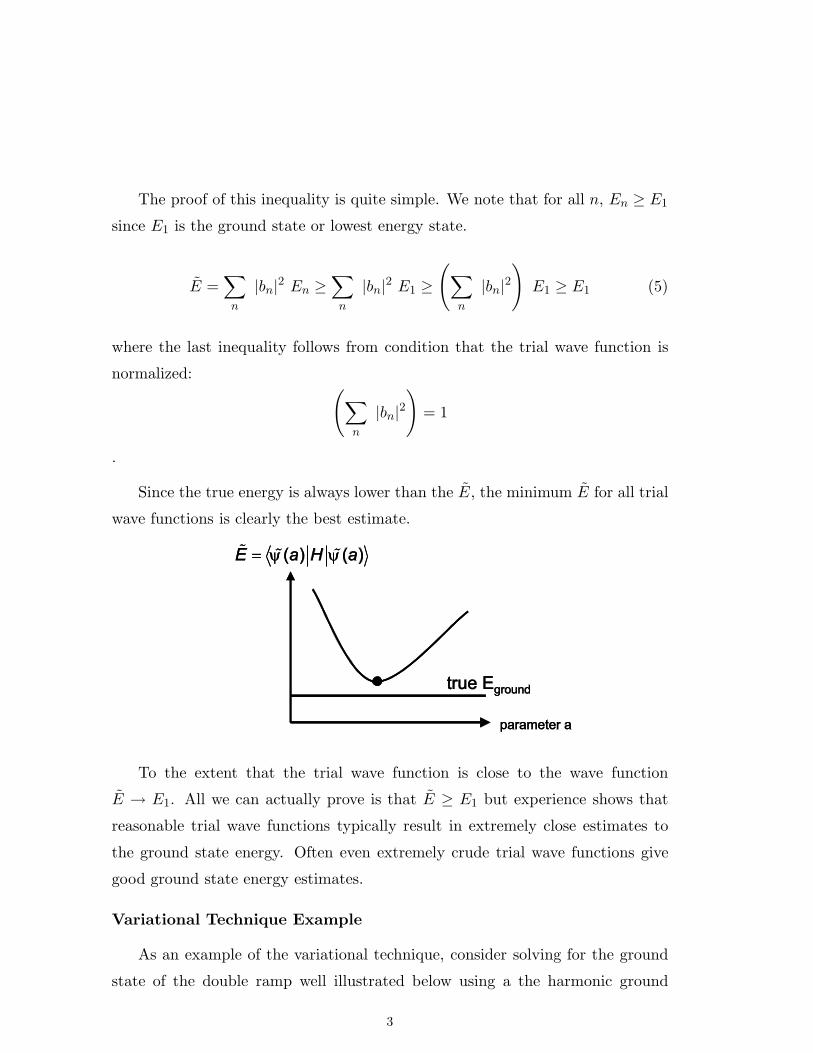
Since the true energy is always lower than the E, the minimum E for all trial

wave functions is clearly the best estimate.

To the extent that the trial wave function is close to the wave function

E → E1. All we can actually prove is that E ≥ E1 but experience shows that

reasonable trial wave functions typically result in extremely close estimates to

the ground state energy. Often even extremely crude trial wave functions give

good ground state energy estimates.

Variational Technique Example

As an example of the variational technique, consider solving for the ground

state of the double ramp well illustrated below using a the harmonic ground

3

state: ψ0 =(√

aπ

)1/2 exp(−ax2

2

)where a is the adjustable parameter which is

inversely related to the width of the wave function.

~

F|x| F | x|

x

V(x)ψ

1/a

2 /2)2xexp(-a=

Our job is to evaluate 〈H〉 = 〈T 〉+〈V 〉. To evaluate 〈V 〉 we will need integals

of the form Jn =∫ +∞0 dy yne−ay2

. These differ from our previous integrals that

appear in the Bound States chapter since they involve odd powers of x and are

integrated from 0 → ∞ rather than from −∞ → ∞. We can get any ”odd”

integrals we need by starting with

J1 =12a−1 and the recursion relation Jn+2 = −∂Jn

∂a

We begin with

〈V 〉 = 〈F |x|〉 = 2(√

a

π

) ∞∫0

dxF x exp(−ax2

)= 2

(√a

π

)F J1 =

F√πa−1/2

We next compute the 〈T 〉. This can in principle be done by brute force

〈T 〉 =h2

2m

⟨ψ0

∣∣∣∣ ∂2

∂x2

∣∣∣∣ψ0

⟩

It is apparent, that 〈T 〉 only involves derivatives and integrals of the trial wave

function and thus can only depend on the shape parameter a and the mass of

4

the particle m and will thus be independent of the potential well. We can thus

exploit the fact that ψ0 is the ground state of a harmonic oscillator which allows

us to compute the kinetic energy very easily by the virial theorem for a harmonic

oscillator wave function: 〈T 〉 = Eo/2 = hω/4. But what ω corresponds to our

trial wave function a parameter? Fortunately this is easy since a = mω/h for the

harmonic oscillator wave function. Hence

〈T 〉 =hω

4=(h

4

)(ha

m

)=h2a

4m

We can now write the E for the trial wave function

E = 〈H〉 =h2a

4m+

F√πa−1/2

The formation of a minimum E is very easy to understand. As a is increased, the

ψ0 becomes narrower and more peaked. Hence its double derivative or kinetic

energy increases. At the same time, the narrowing of ψ0 means that ψ0 probes

closer to the bottom of the well where the potential is lower. There is clearly a

happy balance between lowering the kinetic energy at the expense of raising the

potential.

Minimizing with respect to a we have:

∂E

∂a=

∂

∂a

{h2a

4m+

F√πa−1/2

}= 0 → h2

4m=

F

2√π

a−3/2∗ → a∗ =

(2mFh2√π

)2/3

Inserting a∗ into our expression for E and performing some algebra we have:

E =(

2716π

)1/3 (hF√m

)2/3

It would certainly be great to check our variational estimate for ground state

energy against the true ground state energy. Unfortunately I don’t know the exact

5

answer. We can get some confidence in the answer by comparing the inflection

point of our ψ0 solution to the classical turning point for the two ramp system.

If we had the true solution, the inflection point would equal the turning point.

Recall at the classical turning point E = V and ∂2ψ/∂x2 = 0. The inflection

point of our trial wave function occurs at:

∂2

∂x2e−ax2/2 = (−a+ a2x2) e−a2x2/2 = 0

→ xinflect =1√a

=

(√πh2

2mF

)1/3

= 0.961

(h2

mF

)1/3

(6)

Lets next compute the x coordinate of the classical turning point:

E =(

2716π

)1/3 (hF√m

)2/3

= V = F xturn

or xturn =(

2716π

)1/3(h2

mF

)1/3

= 0.813

(h2

mF

)1/3

Both the classical turning point and inflection point are in reasonable agreement.

It would be very surprising if they were in perfect agreement since a Gaussian

wave function is the correct ground state for an V (x) = K x2/2 potential which

goes to infinity much faster than the linear potential V (x) = F |x| being consid-

ered here.

Just a quick review of the variational strategy. The best bet is to pick a

trial wave function that that is the normalized, ground state of a physical system

that solves a potential similar to that of the novel problem at hand. The virial

theorem will then allow one to quickly write down the kinetic energy part of the

Hamiltonian and avoid all of the work of taking the double derivative of ψ and

then integrating. One is left with doing a single integral over the new potential

in order to set up E and the minimization can frequently be done analytically.

6

One could get better estimates of the true ground state by allowing for more

adjustable parameters. For example in this problem, one could add in another

ground state oscillator contribution, with another adjustable shape parameter

and a third parameter that gives the relative contribution of each ground state

oscillator wave function.

Perturbation versus Variation

Recall that the first order perturbation estimate of the energy when a “small”

perturbation ∆V is added to a Hamiltonian with a known solution Ho is En ≈E0

n + 〈n|∆V |n〉 where |n〉 is the unperturbed state that satisfies Ho|n〉 = E0n|n〉.

We can cast this solution in a form that resembles the variational method:

En = 〈n|H|n〉 = 〈n|Ho + ∆V |n〉 (7)

Now since Ho|n〉 = E0n|n〉 we have 〈n|Ho|n〉 = E0

n we can write Eq. (7) in the

form:

En = 〈ψ|H|ψ〉 = 〈n|H|n〉 = E0n + 〈n|∆V |n〉 where ψ ≡ |n〉 (8)

The interpretation of Eq. (8) is that first order perturbation theory is equivalent

to a variational estimate where the trial wave function is the solution to the un-

perturbed Hamiltonian. The usual case is we are trying to find the ground state

using the variational technique and as discussed above, we always overestimate

the true ground state energy. Eq. (8) then tells us that since first order pertur-

bation theory is equivalent to a variational estimate, the first order perturbation

theory calculation is always an overestimate of the true ground state energy. If

we allow a shape parameter in ψ instead of fixing it to |n〉 we should nearly

always get closer to the true answer than the first order perturbative estimate.

Using ψ100(r) as the ψ(r) in 3-d problems

Often trial wave function based on the hydrogen ground state wave function

is a convenient choice in 3 dimensional problems with spherically sysmmetric

7

potentials.

ψ100(r) =1√π a3

exp(−ra) (9)

In Eq. (9) we think of a as our adjustable parameter rather than setting a = a0

for hydrogen or a = a0/Z for single electron ion. The main convenience of this

form besides its simplicity is the ability to calculate the kinetic energy term 〈T 〉.If we were to set a = a0, to get the actual hydrogen solutions, we would have the

following relationships between a0 and the ground state energy E1:

a =h

αmc, E1 = −1

2mc2α2 where α =

e2

4πεohc=

1137

(10)

We know that 〈T 〉 can really only depend on a, m and h since:

〈T 〉 =h2

2m

⟨ψ∣∣∇2

∣∣ ψ⟩

and a is the only variable in ψ100. Since 〈E〉 = −〈T 〉 as we show shortly from

the virial theorem, it follows that it must be possible to eliminate α and write E

as a function of a, m and h:

α =h

amc, E = −1

2mc2α2 = −1

2mc2

(h

amc

)2

= − h2

2ma2(11)

Our trial wave function is a solution to the Coulomb potential and hence we can

use the virial theorem to relate 〈T 〉 to the total energy E. According to the radial

version of the virial theorem < T >=< r dVdr > /2. For the case of a 1/r potential

< T >=< r dVdr > /2 = −〈V 〉/2. Hence < T > −2 < T >= E or 〈T 〉 = −E.

Hence:

〈T 〉 = −E =h2

2ma2=

h2

2ma20

(a0

a

)2= −E1

(a0

a

)2(12)

The last equality, which is particularly useful in atomic problems, follows from

the observation that if a = a0 then E = E1 = −13.6 eV . Another useful result

8

that we will need shortly also follows from the virial theorem.

⟨1r

⟩=

1a

(13)

This is based on the observation that:

E = − e2

4πεo(2a)(14)

which you can obtain by manipulating the results in Eq. (10). You then use the

virial theorem result 〈V 〉 = −2〈T 〉 and the potential expression for a hydrogen

atom [ V = e2/(4πεo r)] to obtain:

− e2

4πεo(2a)= 〈T 〉 + 〈V 〉 = −〈V 〉

2+ 〈V 〉 =

〈V 〉2

=12

⟨e2

4πεor

⟩→⟨

1r

⟩=

1a

Again this will be true of any solution of the hydrogen ground state and will thus

be true for our trial wave function. We are now very well set up to tackle helium.

The Helium Ground State

The problem of estimating the helium ground state energy is becoming a

classic illustrative problem in the variational technique in quantum mechanics

courses since one gets a value close to the experimental answer, and the problem

can be done analytically - albeit using some clever tricks.

For the chemically challenged, helium has two electrons orbiting about a Z =

2 nucleus. The ground state energy is the total energy of these two electrons which

is less than zero. We can measure this energy by measuring the minimum energy

required to remove both electrons to leave a helium nucleus and two electrons

at rest at infinity. Experimentally it takes 24.6 eV to remove one electron from

a neutral He atom leaving singly ionized He+. Since He+ is a single electron

atom with n = 1 we can reliably compute its energy from the Bohr formula. The

9

ionization energy for the He+ ion is then Z2 13.6 = 4× 13.6 = 54.4 eV . Hence it

takes 54.4+24.6 = 79 eV to remove both electrons. This means the experimental

value for the He ground state is −79 eV .

The helium Hamiltonian is given by:

H = − h2

2m(∇2

1 + ∇22

)− e2

4πεo

(2r1

+2r2

− 1|�r1 − �r2|

)(15)

The factors of 2 come from the nuclear charge. You can easily spot the kinetic

energy terms. The fact that there are 3 particles in the final state means that

there is no obvious reduced mass so we work in the limit of an infinite mass

nucleus. The last term represents the Coulomb repulsion energy between the two

electrons.

In the absence of the 1/|�r1 − �r2| term, the two electron Hamiltonian is just

H = H1 + H2, the ground wave function would be just the direct product:

ψ(�r1, �r2) = ψ100(r1) ψ100(r2)↑1↓2 − ↓1↑2√

2

and the energy would just be E = E(1) + E(2) where E(1),(2) are the energies

of a single electron helium ion in the ground state or −54.4 eV for a total of

−108.8 eV .† Since the true ground state energy of helium is -79 eV the electron-

electron repulsion must be important.

Our approach will be to construct a trial, two electron wave function of the

form: Ψ(�r1, �r2) = ψ100(r1) ψ100(r2) where we use the floating a form given by

Eq. (9). If we set a = a0/Z = a0/2 and use this to evaluate 〈Ψ|H(r1, r2)|Ψ〉 we

will be effectively doing a first order perturbation calculation as described in the

previous section.

† Since the two electrons are identical Fermions, we put the electrons in an antisymmetricspin state with S = 0.

10

If we vary a , to get the minimal E, we are pretty much guaranteed to get a

more accurate answer since the E will be lower with an adjustable compared to

a fixed a parameter and thus closer to the true value.

If we use a = a0/2, we would estimate the ground state energy as:

Eg = 8E1+e2

4πεo< ψ100(�r1)ψ100(�r2)| 1

|�r1 − �r2| |ψ100(�r1)ψ100(�r2) >= 8E1+ < ∆V >

(16)

Although it is surprising how well this approach will work, we clearly seem to

be in a regime where perturbation theory is unreliable given we know the correct

result is -79 eV and the zero order answer is -108.8 eV.

Essentially the bulk of the drudge work is in the calculation of 〈Ψ|∆V |Ψ〉.We will pursue this calculation and then show how we can use the 〈Ψ|∆V |Ψ〉 in

a true variational calculation where we put some adjustable parameters in Ψ.

Computing the ∆V integral

I would have guessed that this 6 dimensional integral is intractable like most

integrals but it can actually be done using an elegant technique. The 〈∆V 〉integral is just 〈∆V 〉 = [e2/(4πε0)] 〈|�r1 − �r2|−1〉 We can be fairly confident that

〈|�r1 − �r2|−1〉 = ξ/a where ξ is a dimensionless number since a is the only length

scale involved with our trial wave function. We will work out the integral in full

detail, just to prove it can be done, but the integral is considerably beyond the

skills of most undergraduates, graduates, or Professor’s who aren’t working in

this branch of computational atomic physics. Our conclusion will be ξ = 5/8 but

getting there is half the fun.

To compute < |�r1 − �r2|−1 > we write |�r1 − �r2|2 in the spherical variables we

will use for the integration.

|�r1 − �r2|2 = (�r1 − �r2) · (�r1 − �r2) = r21 − 2�r1 · �r2 + r22 = r21 − 2r1 r2 cos θ12 + r22

11

where θ12 is the angle between �r1 and �r2. We next insert the ψ100 wave functions

ψ100 =1√π a3

e−r/a

< ∆V >=e2

4πεo

(1

a6 π2

) ∫d3r1 d

3r2e−2r1/a e−2r2/a√

r21 − 2r1 r2 cos θ12 + r22

=e2

4πεo

(1

a6 π2

)I

We note that the ψ100 expression appears four times in the integral (twice in the

bra and twice in the cket) hence some of the surprising numerical factors. We

begin by partitioning the integral as an integral over r1 and �r2.

I =∫d3r1 e

−2r1/a I2(�r1) , I2(�r1) =∫d3r2

e−2r2/a√r21 − 2r1 r2 cos θ12 + r22

(17)

We note that the inner I2 integral will have a dependence on �r1 and no

dependence on �r2 since that is being integrated over. Part of this dependence

will come from the r1 (1st electron radial coordinates) under the √, the other

piece looks like it will come from cos θ12 piece. Now we introduce a famous trick.

We have a double integral. The first integral involves varying �r1 over all of its

space. However in performing the inner integral, one is essentially varying �r2 over

all space but keeping �r1 fixed. Now the trick is since �r1 is fixed, why not use it to

define z direction during the evaluation of the I2 integral? If we do this, we can

equate cos θ12 with the cos θ that desribes �r2 since if �r1 is in the same direction

as z , θ12 will be the usual angle of �r2 with respect to the z axis. We then have:

I2(�r1) =

∞∫0

r2 dr e−2r/a

1∫−1

d cos θ√r21 − 2r1 r cos θ + r2

2π∫0

dφ (18)

The φ integral is just 2π. The θ integral is very easy. Just substitute v =

r21 + r2 − 2rr1 cos θ. Then d cos θ = dv/(−2rr1) and the limits become v1 =

r21 + r2 + 2rr1 = (r1 + r)2 and v2 = (r1 − r)2

12

Iθ =

1∫−1

d cos θ√r21 − 2r1 r cos θ + r2

→ −12rr1

v2∫v1

v−1/2dv

=−1rr1

(√v1 −√

v2) =(r1 + r) − |r1 − r|

rr1=

{2/r1 if r < r1

2/r if r > r1

The last equality is sort of interesting and follows from |r1 − r| is either r1 − r

or r − r1 depending on the magnitude of r versus r1. The conditional is easy to

insert by breaking up Eqn. (18) into 2 pieces:

I2(�r1) = 4π

r1∫

0

r2 dre−2r/a

r1+

∞∫r1

r2 dre−2r/a

r

=

πa3o

r1

[1 −

(1 +

r1a

)e−2r1/a

]

The exponential integrals can be found in any integral table. We can now insert

I2(r1) into Eqn. (17).

I =∫d3r1 e

−2r1/a I2(r1) = 4π2a3

∞∫0

r21dr1 e−2r1/a 1

r1

[1 −

(1 +

r1a

)e−2r1/a

]

Since I integrand has no angular dependence, the angular pieces integrate to 4π.

The remaining r1 integral is very easy using∫∞0 dy yn exp(−by) = n!/bn+1 to

get:

I = 4π2a3 5a2

32= or < ∆V >=

e2

4πεo

(1

a6 π2

)× 4π2a3 5a2

32=

58a

(e2

4πε0

)

< ∆V >= −54

(− e2

4πε0 (2a)

)= −5

4

(− e2

4πε0 (2a0)

) (a0

a

)

Thus < ∆V >= −54E1

(a0

a

)(19)

If we insert a = a0/2 we get < ∆V >= −5E1/2 = +34 eV . We estimate from the

forgoing that the helium ground state energy is Eg < −108.8 + 34 = −74.8 eV .

13

We are thus much closer to the true answer of -79 eV which is remarkable given

either the size of the perturbation or the fact that we used a very naive wave

function which ignores the electron-electron repulsion.

Improving our Bound

We can do better by allowing a to vary. I find it more instructive to write

a = a0/Z and allow Z = Zeffective to be the adjustable parameter. This is a

nice approach since we can think of the Coulomb repulsion of the other electron,

as creating a “shielded” nuclear charge for a given electron. As such we might

expect an effective nuclear charge of Z < 2 and which will place the electrons

further away that we were assuming before with our Z = 2 Bohr wave functions.

Our goal is to compute E from Eqn(15) which gives the true helium Hamil-

tonian:

E = 〈Ψ|T1 + T2|Ψ〉 − e2

4πεo

(2⟨

Ψ∣∣∣∣ 1r1

+1r2

∣∣∣∣Ψ⟩−⟨

Ψ∣∣∣∣ 1|�r1 − �r2|

∣∣∣∣Ψ⟩)

(20)

where T1,2 = − h2

2m∇2

1,2

You will recognize the last term as < ∆V > which we computed in the previous

section in Eq. (19):

< ∆V >= −54

(a0

a

)E1 = −5Z

4E1 (21)

We next compute one of the kinetic energy terms:

〈Ψ(�r1, �r2)|T1|Ψ(�r1, �r2)〉 = 〈ψ100(�r1)|T1|ψ100(�r1)〉〈ψ100(�r2)|ψ100(�r2)〉 = 〈ψ100(�r)|T |ψ100(�r)〉

〈T1〉 =h2

2ma2= Z2 h2

2ma20

= −Z2E1

〈T1 + T2〉 = 2〈T1〉 = −2 Z2E1 (22)

where we have used Eq. (11) to equate E1 with −h2/(2ma20) and the fact that

the two electrons are indistinquishable to conclude 〈T1〉 = 〈T2〉.

14

The same reasoning tells us us 〈1/r1〉 = 〈1/r2〉. Using Eq. (13) we have

〈1/r1〉 = 〈1/r2〉 = 1/a = Z/a0. Hence the second term of Eq. (20) representing

the attraction of the two electrons to the nucleus is:

− e2

4πεo

(2⟨

Ψ∣∣∣∣ 1r1

+1r2

∣∣∣∣Ψ⟩)

= −4Ze2

4πεoa0= 8ZE1 (23)

Assembling Eq. (21) - Eq. (23), we have:

E = −2Z2E1 + 8ZE1 − 5Z4E1 =

(−2Z2 +

274Z

)E1

We thus obtain a classic concave up parabola (remember E1 is negative) with

a minimum at dE/dZ = (−4Z + 27/4)E1 = 0 or Z = 27/16 = 1.69 or Emin =

(36/27)E1 = −77.5 eV which is getting pretty close to the experimental value of

-79 eV. Our first order calculation where we set Z = 2 placed us 4.2 eV above

the true value. By allowing Z to be an adjustable parameter in a variational

calculation, we are now only 1.5 eV above the experimental value. We have thus

shrunk the gap between calculation and observation by a factor of 2.8 with very

little additional work.

The Z value is quite sensible as well. Without the additional electron, a given

electron would see Z = 2. If the additional electron provided perfect shielding

we would have Z = 1. A value of Z = 1.69 seems quite reasonable.

Although this problem is solveable analytically , it would not be that difficult

to perform even the 6 dimensional< ∆V > integral on a computer by summation.

Essentially we know that 〈|�r1 − �r1|−1〉 which is the essence of the < ∆V >

calculation must be of the form 〈|�r1 − �r1|−1〉 = ξ/a where ξ is a numerical

constant since a is the only thing in our Ψ that carries dimensions of length. All

of the clever analytic integration did was to establish that ξ = 5/8. It is likely to

be simpler and faster to write such a program to do the calculation numerically

from the get go. But there is a sense of accomplishment in doing the seemingly

15

impossible analytic calculation. I do hope you find you are able to follow the

basic QM that we used in this example.

The H+2 Molecule

In this section we summarize a variational calculation on the binding energy

H+2 where an electron “orbits” about two protons to form the simplest molecule.

This was one of the earliest attempts to understand the nature of a covalent

bond performed within a few years after the development of the Schrodinger

Equation. I will leave out many of the mathematical details which are discussed

in Griffiths and other quantum mechanics books such as Quantum Mechanics

by Goswami and Quantum Physics by Gasiorowicz. We are describing a

“covalent” bond. There are also ionic bonds in chemistry.

This calulation is concerned with whether or not the H+2 molecule will even

exist. How does the “orbiting” electron’s attraction to either proton, overcome

the Coulomb repulsion between the two protons to form a bound state i.e. a

state with negative energy? Actually the existence of a negative energy state is

really not enough by itself since the molecular configuration must be energetically

favored over a final state consisting of a hydrogen atom plus a free proton. This

means the system must have a total energy of less than E1 or -13.6 eV. It is

really not all that obvious a priori that the H+2 ion should exist. For example

in the upper part of the below figure we placed the electron half way between

the two protons which are separated by 2a0. Adding the potential energies we

find a net potential energy of 3E1 = −40.8 eV which is considerably smaller

than E1 = −13.6 eV suggesting that this configuration lies considerably lower in

energy than a hydrogen atom with an additional proton infinitely far away and

at rest. Of course we need to worry about the fact that the elecron has a kinetic

energy which will raise its energy, perhaps by 〈T 〉 = −E1. It is still plausible

that if the electron were often between the two protons as shown, the hydrogen

molecule might bind even when kinetic energy is considered.

Of course, the electron cannot be precisely located between the two protons

16

but is described by a probability function that extends over all space.

For example the electron could easily be in the position shown in the lower

half of the above figure. In this position the sum of the potential energies is just

E1 which is the same energy as single hydrogen atom with a distant proton at

rest. When kinetic energy is taken into account the electron would bind into

a hydrogen atom rather than forming a molecule with the two protons in this

case. To really know if the H+2 molecule exists we need a legitimate quantum

mechanical calculation which we will base on a variational approach.

Here is the essence of our variational approach. We will place the two protons

a distance R apart and assume they are “nailed” down at these positions. This

will give a positive proton-proton repulsion contribution of

Vpp =e2

4πεoR=

−2ao

R

−e24πεo2ao

= −2ao

RE1

to the total binding energy.† The electron will then have a Hamiltonian given

† It also seems by nailing down the protons we are ignoring their own quantum physics suchas the fact that need to move about to conform to the uncertainty principle. My guess (asa non-expert) is this sort of kinetic energy < p2/2M > may be may be ignorable owing tothe large proton mass.

17

by

H = − h2

2m∇2 − e2

4πεo

(1r1

+1r2

)(24)

where r1 and r2 are shorthands for r1 = |�r − �R1| and r2 = |�r − �R2|, �r is the

coordinate of the electron where �R1, and �R2 are the positions of the two protons

and R = |�R2 − �R1|. Our approach will be to use a trial wave function (Ψ),

compute E =< Ψ|H|Ψ > +Vpp and vary R looking for the minimum of E. If

we agree with the fixed R assumption, the true energy will lie below E hence if

E < −13.6 eV the molecule will form.

We will use a linear combination of the atomic orbits (known LCAO) as our

trial wave function based on the hydrogen ground state. Specifically we will use:

Ψ(�r) = N(ψ100(|�r − �R1|) + ψ100(|�r − �R2|)

)= N (ψ(r1) + ψ(r2))

This Ψ is again motivated for mathematical convenience and physical intu-

ition. We are saying the electron has an equal probability of being in a ground

state hydrogen centered about either proton in the molecule. These wave func-

tions satisfy the Schrodinger equation of a very similar Hamiltonian which cuts

down on the mathematical drudgery. The factor N reflects the fact that we have

a non-trivial normalization. Now it is apparent from symmetry that we want an

equal probability for being attached to either proton but we could also achieve

this with any arbitrary unimodular phase: Ψ = N (ψ(r1) + exp(iδ)ψ(r2)).

Actually the only two possible choices are exp(iδ) = ±1 because the Hamilto-

nian has r1 ↔ r2 symmetry which we will define in terms of a symmetry operator:

χψ(r1, r2) = ψ(r2, r1). This suggests that the wave function can be chosen to be

a simultaneous eigenfunction of χ and x. Writing the eigenvalue of χ as λ we

have: χ2ψ(r1, r2) = ψ(r1, r2) = λ2ψ(r1, r2) which implies λ2 = 1 or λ = ±1. This

18

means

χ (ψ(r1) + exp(iδ)ψ(r2)) = (ψ(r2) + exp(iδ)ψ(r1)) = ± (ψ(r1) + exp(iδ)ψ(r2))

Solving this we see the only two phase choices are exp(iδ) = ±1. It turns out

that our initial phase choice (δ = 0) gives the best bound. You will explore the

other choice ( δ = π ) in the exercises.

Lets begin with the normalization

N 2 〈ψ(r1) + ψ(r2) | ψ(r1) + ψ(r2)〉 = 1 = N 2 (2 + 2 < ψ(r1)|ψ(r2) >)

We use the fact that

< ψ(r1)|ψ(r1) >=< ψ(r2)|ψ(r2) >= 1 , < ψ(r1)|ψ(r2) >=< ψ(r2)|ψ(r1) >

The first relation follows for the atomic orbital normalization. The second follows

from the fact that the wave functions are real. We often call < ψ(r1)|ψ(r2) >≡ I

the “overlap” integral. One form for this, where we put one proton at the origin

and the other on the z axis , would be:

I =1πa3

o

∫d3r exp

(− r

ao

)× exp

(−|�r −Rz|

ao

)

Clearly the overlap integral I can only depend on R and ao and in fact only

depends on the ratio ξ = R/ao. One can show (although its not trivial) that:

I = exp(−ξ)(

1 + ξ +ξ2

3

)and N =

1√2(1 + I)

(25)

We can now proceed to construct E using the Hamiltonian given by Eqn.

(24). However, our wave function is constructed from hydrogen wave functions

19

which are eigenfunctions of pieces of the Hamiltonian. Hence for example:

Hψ(r1) =

{− h2

2m∇2ψ(r1) − e2

4πεo1r1ψ(r1)

}− e2

4πεo1r2ψ(r1)

The piece of the Hamiltonian within the {} is the Hamiltonian for a hydrogen

atom displaced by �R1 acting on a similarly displaced ψ100(�r − �R1). It will thus

return the usual energy E1ψ(r1). Hence:

Hψ(r1) = E1ψ(r1)− e2

4πεo1r2ψ(r1) and similarly Hψ(r2) = E1ψ(r2)− e2

4πεo1r1ψ(r2)

Thus HΨ = N H [ψ(r1) + ψ(r2)] or:

HΨ = E1Ψ −N e2

4πεo

(1r2ψ(r1) +

1r1ψ(r2)

)

Hence:

E =< Ψ|H|Ψ >= E1 < Ψ|Ψ >

−N 2 e2

4πεo

(⟨ψ(r1) + ψ(r2)

∣∣∣∣ 1r2∣∣∣∣ψ(r1)

⟩+⟨ψ(r1) + ψ(r2)

∣∣∣∣ 1r1∣∣∣∣ψ(r2)

⟩)

Taking advantage of some r1 ↔ r2 symmetries:

E = E1 − 2N 2 e2

4πεo

(⟨ψ(r1)

∣∣∣∣ 1r2∣∣∣∣ψ(r1)

⟩+⟨ψ(r1)

∣∣∣∣ 1r1∣∣∣∣ψ(r2)

⟩)

E = E1 − 4N 2 e2

4πεo2ao

(⟨ψ(r1)

∣∣∣∣ao

r2

∣∣∣∣ψ(r1)⟩

+⟨ψ(r1)

∣∣∣∣ao

r1

∣∣∣∣ψ(r2)⟩)

E = E1+4E1N 2(D+X) whereD =⟨ψ(r1)

∣∣∣∣ao

r2

∣∣∣∣ψ(r1)⟩

andX =⟨ψ(r1)

∣∣∣∣ao

r1

∣∣∣∣ψ(r2)⟩

where D and X are dimensionless positive integrals which can be worked out

20

analytically but are non-trivial:

D =1ξ−(

1 +1ξ

)e−2ξ , X = (1 + ξ)e−ξ where ξ = R/ao (26)

We note that the two integralsX , I that are based on< ψ(r1)| anything |ψ(r2) >

fall off as exp(−R/ao) as ξ → ∞ as one might expect since the Bohr ground

state wave functions fall off exponentially as R/ao. We can take D(ξ) to the

R = |�R| → ∞ by realizing �r2 − �r1 = �R thus �r2 = �r1 + �R→ �R and

D =⟨ψ(r1)

∣∣∣∣ao

r2

∣∣∣∣ψ(r1)⟩

→⟨ψ(r1)

∣∣∣ao

R

∣∣∣ψ(r1)⟩

=ao

R=

1ξ

which is borne out by Eq. (26).

Another check is to go to the opposite limit where ξ → 0 or R → 0. In this

limit r2 → r1. Hence

I(ξ) → 〈ψ(r)|ψ(r)〉 = 1 ; D(ξ) → I(ξ) →⟨ψ(r)

∣∣∣ao

r

∣∣∣ψ(r)⟩

= a0

⟨1r

⟩= 1

where we use the result from Eq. (13) that 〈r−1〉 = a−10 . Indeed the forms for all

three functions Eq. (25) and Eq. (26) approach 1 as ξ → 0, although one must

take some care in taking D(ξ) to this limit.

Including the Vpp term, and inserting our expression for N 2 in terms of third

non-trivial integral (I) we have our total energy E

E = E + Vpp = −2ξE1 + E1 + 2E1

D +X

1 + I

Collecting the expressions for the D , X , I integrals we have:

f(ξ) =E

−E1= −1 +

2ξ

((1 − (2/3)ξ2

)e−ξ + (1 + ξ) e−2ξ

1 + (1 + ξ + (1/3)ξ2) e−ξ

)

As ξ → ∞ all three integrals D , X , I vanish as does Vpp and E → E1. This

makes perfect sense since as R → ∞ we are essentially left with a superposition

21

of a hydrogen atoms and a free proton. As R → 0 the Vpp term dominates and

E → +∞. But between these two extremes we have E < E1 with a minimum near

E = −13.6−1.76 eV . The 1.76 eV would be our bound on the molecular binding

energy for the H+ ion. Because this is a variational calculation we know this ion

is more tightly bound and in fact has a binding energy of 2.8 eV implying an

actual energy lower than E . Our estimate was not a great estimate of the binding

energy, indicating our trial wave function wasn’t that realistic. Our minimizing

R is at 1.27 A whereas experimentally the number is closer to 1.06 A. We could

do much better by putting some adjustability in out trial wave functions. But

at least its plausible that molecules will form as stable entities. Given we are

constructed from molecules its good we proved the simplest one exists! Here is

a crude sketch of ours and a much more sophisticated molecular calculation that

agrees with the experimental values.

-13.6 eV R

1.3 A

1.06 A

.

.

energy

2.8 eV

1.76 eV

In the exercises I ask you to consider binding of an alternative trial wave

function Ψ = N (ψ100(r1) − ψ100(r2)) where the normalization is different. I

think you will find that this wave function will not bind. I think the reason is

that with this relative phase, the trial wave function vanishes on the plane where

r1 = r2 and therefore cannot take advantage of the large binding contribution

near this plane. These are called “anti-bonding” orbitals and play an important

role in understanding molecular dynamics in chemical processes.

22

Although we know our variational calculation is not terribly accurate it does

resemble more accurate calculations of the binding energy versus the atomic

separation R. At some risk, I have crudely represented the energy near the

minimum by the dashed parabola shown above to find an effective spring constant

of k = 500 eV/nm2 where the parabola is given by E = kx2/2 − Emin. We

can roughly think of the two protons as interacting through the approximate 1

dimensional simple harmonic oscillator Hamiltonian of the form

H =−h2

2µ∂2

∂x2+

12kx2

where x = x1 − x2 is a relative coordinate and ω =√k/µ where µ = M/2 is

the reduced mass for two protons. We thus expect a set of vibrational molecular

levels separated by energies of ∆E = hω or

∆E = hc

√2kMc2

= 197eV nm

√2 × 500 eV/nm2

940 × 106 eV= 0.203 eV

where we used 940 × 106 eV as Mc2 for a proton. Indeed one does typically

get a series of roughly evenly spaced infrared absorption and emission lines at

energies on the order of a few hundredths to a few tenths of an electron volt due

23

to molecular vibrations. Typically , as in this case, the level spacing will get

smaller for the more highly excited states since the well is only approximately

parabolic.

Another feature of molecular aborption or emission spectra are rotational

excitations. We can think of the H2 molecule as a rigid rotator with a moment

of inertia given by µR2 that can be in various L2 states. The kinetic energy will

then be of the form:

E� =�(�+ 1)h2

2µR2= �(1+�)

(197 eV nm)2

2 12(940 × 106 eV ) (0.13 nm)2

= �(�+1) 2.4×10−3 eV

where we have used the minimum of our admittedly crude potential well calcula-

tion as a bond length of 0.13 nm. In fact measuring the energy level spacing due

to rotational excitations of molecules is a frequently used method for measuring

bond lengths – which of course play a crucial role in constructing chemical models

of molecules.

Hence superimposed on the infrared absorption spectra due to vibrational

modes will be a series of even closer spaced rotational spectrs.

Important Points

1. We discussed the use of a variational technique to compute the approximate

energy of a quantum mechanical ground state. The technique requires

you to guess a “reasonable” trial wave function, ψ(x), with at least one

adjustable (shape) parameter. The wisest choice is to pick an actual of

ground state of a related system such as a harmonic oscillator ground state.

We proved the inequality:

E = < ψ|H|ψ > > Eground

In computing E one must be careful to include both the kinetic and po-

tential energy terms. If one chooses a ground state of a related system the

24

kinetic energy can be written down very easily using the virial theorem.

The minimum value of E (as its parameters are varied) generally provides

a good estimate for the true ground state energy of the system.

2. We applied the variational technique to the helium ground state. The

complication to the quantum mechanics of helium is the electron-electron

repulsion term. For this problem we used the product of two shielded

hydrogen atom ground state orbit to act as a two particle trial wave function

and got within 2% of the experimental result and a reasonable result for

the shielded nuclear charge.

3. We computed the binding energy of the H+2 molecule where an electron

orbits about two protons. We did the calculation by placing the two protons

a distance R apart and then tried a trial wave function of the form Ψ ∝ψ100(r1)+ψ100(r2) where r1 is the distance of the electron to one proton and

r2 is the distance of the electron to the other. This is sometimes called a

LCAO approach or linear combination of atomic orbitals. We found that it

was indeed possible to get a variational estimate that had the total energy

of the system (including the Coulomb repulsion between the two protons)

less than -13.6 eV which means the molecule has a smaller energy than

a hydrogen atom and free proton. We varied the R separation between

the two protons but did not vary the LCAO wave function. The molecular

binding energy was rather small and not terribly accurate but we concluded

that molecules exist.

4. Finally we showed how the E versus R curve can be used to crudely es-

timate bond lengths and effective spring constants that can be used to

estimate the vibrational and rotational energy levels of diatomic molecules.

Typically the vibrational levels absorb infrared photons and the rotational

levels absorb far infrared photons.

25