Variational Autoencoders for Deforming 3D Mesh Models

Qingyang Tan1,2, Lin Gao1∗, Yu-Kun Lai 3, Shihong Xia1∗

1Beijing Key Laboratory of Mobile Computing and Pervasive Device,

Institute of Computing Technology, Chinese Academy of Sciences2School of Computer and Control Engineering, University of Chinese Academy of Sciences

3School of Computer Science & Informatics, Cardiff University

tanqingyang14@mails.ucas.ac.cn, {gaolin, xsh}@ict.ac.cn, LaiY4@cardiff.ac.uk

Abstract

3D geometric contents are becoming increasingly pop-

ular. In this paper, we study the problem of analyzing de-

forming 3D meshes using deep neural networks. Deforming

3D meshes are flexible to represent 3D animation sequences

as well as collections of objects of the same category, al-

lowing diverse shapes with large-scale non-linear deforma-

tions. We propose a novel framework which we call mesh

variational autoencoders (mesh VAE), to explore the prob-

abilistic latent space of 3D surfaces. The framework is easy

to train, and requires very few training examples. We also

propose an extended model which allows flexibly adjusting

the significance of different latent variables by altering the

prior distribution. Extensive experiments demonstrate that

our general framework is able to learn a reasonable rep-

resentation for a collection of deformable shapes, and pro-

duce competitive results for a variety of applications, in-

cluding shape generation, shape interpolation, shape space

embedding and shape exploration, outperforming state-of-

the-art methods.

1. Introduction

With the development of performance capture tech-

niques, 3D mesh sequences of deforming objects (such

as human bodies) become increasingly popular, which are

widely used in computer animation. Deforming meshes can

also be used to represent a collection of objects with differ-

ent shapes and poses, where large-scale non-linear defor-

mations are common. There are still challenging problems

to analyze deforming 3D meshes and synthesize plausible

new 3D models. From the analysis perspective, complex

deformations mean it is difficult to embed such 3D meshes

into a meaningful space using existing methods. Acquir-

ing high quality 3D models is still time consuming, since

∗Corresponding Author

multiple scans are usually required to address unavoidable

occlusion. Thus effectively generating plausible new mod-

els is also highly demanded.

In this paper, we propose a novel framework called mesh

variational autoencoders (mesh VAE), which leverages the

power of neural networks to explore the latent space behind

deforming 3D shapes, and is able to generate new models

not existing in the original dataset. Our mesh VAE model is

trained using a collection of 3D shapes with the same con-

nectivity. Many existing deformable object collections sat-

isfy this. They are not restricted to a single deformable ob-

ject; examples include the MPI FAUST dataset [2] which in-

cludes human bodies of different shapes in different poses.

In general, meshes with the same connectivity can be ob-

tained using consistent remeshing. Although convolutional

neural networks (CNNs) have been widely used for im-

age analysis and synthesis, applying them to 3D meshes is

still quite limited. Previous work focuses on generalizing

CNNs from 2D to 3D while preserving image-like regu-

lar grid connectivity, including 3D convolution over vox-

els (e.g. [46]), and 2D convolution over geometry images

(e.g. [37]). However, the voxel representation is inefficient

and given the practical limit can only represent rough 3D

models without details. The parameterization process to

generate geometry images involves unavoidable distortions

and may destroy useful structure information.

Our work aims to produce a generative model capa-

ble of analyzing model collections and synthesizing new

shapes. To achieve this, instead of using representations

with image-like connectivity, we propose to use a state-of-

the-art surface representation called RIMD (Rotation In-

variant Mesh Difference) [9] to effectively represent de-

formations, along with a variational autoencoder [19]. To

cope with meshes of arbitrary connectivity, we propose to

use a fully-connected network, along with a simple recon-

struction loss based on MSE (mean square error). As we

will show later, the large number of coefficients in this net-

work can be efficiently trained, even with a small number of

15841

training examples. We also propose a new extended model

where an additional adjustable parameter is introduced to

control the variations of different latent variables in the prior

distribution. This provides the flexibility of enforcing cer-

tain dimensions in the latent space to represent the most im-

portant differences in the original dataset. As we will show

later, by using an effective feature representation and a suit-

able network architecture, our general framework is able to

produce competitive results for various applications, includ-

ing shape generation, shape interpolation, shape embedding

and shape exploration, outperforming state-of-the-art meth-

ods, where traditionally dedicated methods are needed for

different applications.

2. Related Work

3D Shape Representation and Interpolation. To effec-

tively represent a collection of shapes with the same con-

nectivity, a naive solution is to take the vertex positions as

the representation. Such representations however are not

translation or rotation invariant. Among various represen-

tations, the RIMD representation [9] is translation and ro-

tation invariant, and suitable for data-driven shape analysis.

Therefore, we use it to represent shapes in our framework.

A natural application for shape representations is to in-

terpolate or blend shapes. Existing methods can be largely

categorized into geometry-based (e.g. [14]) and data-driven

(e.g. [8]) methods. The latter exploits latent knowledge of

example shapes, and so can produce more convincing in-

terpolation results when such examples are available. Our

method is a generic framework and as we will show later,

it produces comparable or even better results than state-

of-the-art data-driven methods. Rustamov et al. [33] and

Corman et al. [7] propose map-based methods to describe

distortions between models, which can be used with PCA

(Principal Component Analysis) to produce linear embed-

ding, while our embedding application is non-linear.

Deep Learning for 3D Shape Analysis. In recent years,

effort has been made to generalize image-based CNN mod-

els to analyze 3D shapes. Su et al. [39] and Qi et al. [31]

use multi-view CNN models for 3D object classification.

Li et al. [22] produce joint embeddings of shapes and im-

ages, which are useful for shape-based image retrieval. Shi

et al. [35] propose a method that converts 3D shapes into a

panoramic view, and propose a variant of CNN to learn the

representation from such views. Maturana and Scherer [28]

combine the volumetric occupancy grid representation with

a 3D CNN to recognize 3D objects in real time. Wu

et al. [45] interpret 3D object structure and 2D keypoint

heatmaps from 2D images. Some other works generalize

CNNs from the Euclidean domain to non-Euclidean domain

[3, 27, 5, 4, 26], which is useful for 3D shape analysis such

as establishing correspondences. Maron et al. [25] define a

natural convolution operator on surfaces for CNNs by pa-

rameterizing the surface to a planar flat-torus. Our work

has a rather different focus for analyzing and synthesizing

3D shapes with large deformations, although it may benefit

from [25] to generate consistent meshes. Verma et al. [42]

propose convolutional filters which can be applied to nodes

in a graph with different degrees so can be used in intrinsic

geometry learning. However, their method is suitable for

shape correspondence at the vertex level (surface domain)

rather than the shape level (shape collection domain) and

thus cannot be directly generalized to our problems such

as shape generation and dimensionality reduction. Tan et

al. [40] propose a specific method to analyze sparse de-

formation patterns using CNNs, while our work provides

a more generic framework for various applications.

3D Model Synthesis. Traditional methods for 3D model

synthesis use probabilistic inference. Xue et al. [47] re-

cover 3D geometry from 2D line drawings using examples

and a maximum-a-posteriori (MAP) probability optimiza-

tion. Huang et al. [13] use a probabilistic model to gener-

ate component-based 3D shapes. Such methods are gener-

ally suitable for specific types of 3D shapes. Recent works

consider exploiting the capability of deep learning for 3D

model synthesis. For this purpose, the voxel representation

is resemblance to 2D images and widely used. Wu et al. [46]

propose a generative model based on a deep belief network

trained on a large, unannotated database of voxelized 3D

shapes. Girdhar et al. [10] jointly train an encoder for 2D

images, and a decoder for voxelized 3D shapes, allowing

3D reconstruction from a 2D image. Yan et al. [48] gen-

erate 3D objects with deep networks using 2D images dur-

ing training with a 3D to 2D projection layer. Rezende et

al. [32] learn strong deep generative models for 3D struc-

tures, which is able to recover 3D structures from 2D im-

ages via probabilistic inference. Choy et al. [6] develop a

recurrent neural network which takes in images of an ob-

ject instance from arbitrary viewpoints and outputs a recon-

struction of the object in the form of 3D occupancy grids.

Sharma et al. [34] propose a convolutional volumetric au-

toencoder without object labels, and learn the representation

from noisy data by estimating the voxel occupancy grids,

which is useful for shape completion and denoising. Such

methods however suffer from high complexity of the voxel

representation and can only practically synthesize coarse

3D shapes lack of details.

Sinha et al. [36] propose to learn CNN models using ge-

ometry images [12], which is then extended to synthesize

3D models [37]. Geometry images allow surface details

to be well preserved. However, the parameterization used

for generating geometry images involves unavoidable dis-

tortions and is not unique. This is more challenging for

shapes with complex topology (e.g. high-genus models).

Tulsiani et al. [41] develop a learning framework to abstract

complex shapes and assemble objects using 3D volumetric

5842

primitives. Li et al. [21] propose a neural network archi-

tecture for encoding and synthesizing 3D shapes based on

their structures. Nash et al. [29] use a variational encoder

to synthesize 3D objects segmented into parts. Both [21]

and [29] are designed to synthesize man-made objects and

require part-based segmentation as input, and cannot cope

with unsegmented or deformed shapes addressed in this pa-

per. Such methods can produce shapes with complex struc-

tures, but the level of details is restricted to the components

and primitives used. We propose a general framework that

uses a rotation invariant mesh representation as features,

along with a variational encoder to analyze shape collec-

tions and synthesize new models. Our method can generate

novel plausible shapes with rich details, as well as a variety

of other applications.

3. Feature Representation

In this section, we briefly summarize the feature used

for training neural networks, as well as reconstructing and

generating new models. We use the rotation-invariant mesh

difference (RIMD) feature [9]. We assume that we have

M (M ≥ 2) models, with n vertices that are in one-to-one

correspondence. Generally, the first model is considered as

the reference model and other models are deformed models.

As we will show later, the choice of base mesh does not

affect the results. The deformation gradient Ti at vertex vi(the i-th vertex) can be obtained by minimizing the energy:

E(Ti) =∑

j∈Ni

cij‖e′ij − Tieij‖2, (1)

where Ni is the one-ring neighbors of vertex vi, e′ij =p′

i − p′

j , and eij = pi − pj . pi and p′

i are the positions of

vi on the reference and deformed models, respectively. cijis the cotangent weight cij = cotαij + cotβij , where αij

and βij are angles opposite to the edge connecting vi and

vj . As shown in [20, 9], the cotangent weight is helpful to

avoid discretization bias from underlying smooth surfaces

to meshes. The deformation gradient can be decomposed

into a rotation part and a scaling/shear part as Ti = RiSi,

where the scaling/shear part Si is rotation invariant [17].

The rotation difference dRij from vi to an adjacent vertex

vj cancels out global rotation and is thus also rotation in-

variant: dRij = RTi Rj . The RIMD representation is ob-

tained by collecting the logarithm of the rotation difference

matrix dRij of each edge (vi, vj) and scaling/shear matrix

Si of each vertex vi:

f = {log dRij ; Si} (∀i, j ∈ Ni). (2)

The use of matrix logarithm helps make the feature linearly

combinable. Given a RIMD feature, which can be the out-

put of our mesh VAE, the mesh model can be reconstructed

efficiently by optimizing the energy in Eqn. 1. See [9] for

details. As shown in Table 2 of [9], the mean reconstruction

error between the reconstructed and ground truth shapes is

extremely small (10−4) with no visual difference, which

shows the high representation power of RIMD feature.

4. Mesh VAE

In this section, we introduce our mesh VAE. We first dis-

cuss how to preprocess the feature representation to make

it more suitable for neural networks, and then introduce the

basic mesh VAE architecture, as well as extended models

taking conditions into account for improved control of the

synthesized shapes and with improved embedding capabil-

ity. Finally we summarize a variety of applications.

4.1. Feature Preprocessing

In our architecture, we propose to use hyperbolic tan-

gent (tanh) as the activation function of the probabilistic

decoder’s output layer. The range of tanh is (−1, 1), and

it has the gradient vanishing problem during training when

the output is near −1 and 1. Although alternative activa-

tion function ReLU does not have the gradient vanishing

problem, its range of (0,+∞) is too large. As a generative

model, we expect the network output to be in a reasonable

range. With the limited range of the output, the broad range

of ReLU would make the model difficult to train. The ac-

tivation function tanh is also applied in recent generation

networks [16, 21]. To avoid the gradient vanishing problem

of tanh, we use uniform normalization to preprocess the

feature to the range of [−a, a], where a is close to but not

equal to 1. The preprocessing is a mapping as follows:

fji = 2a×

fji −minj(f

ji )

maxj(fji )−minj(f

ji )

− a, (3)

where fji is the i-th component of model j’s RIMD feature,

fji is the preprocessed feature. If maxj(f

ji ) = minj(f

ji ) for

examples in the dataset, we replace them with fji ± ǫ. Using

a and ǫ also allows the network to generate reasonable mod-

els with features outside the range of the original dataset. In

our experiments, we choose ǫ = 10−6 and a = 0.9.

4.2. Mesh VAE Architecture

Following [19], our mesh VAE aims to find a probabilis-

tic encoder and a probabilistic decoder. The encoder aims to

map the posterior distribution from datapoint x to the latent

vector z, and the decoder produces a plausible correspond-

ing datapoint x from a latent vector z. In our mesh VAE, the

datapoint x is the preprocessed mesh feature f . Denote by

K the dimension of f . For mesh models with 5000 faces,

a typical input RIMD feature dimension is K = 60012.

By default, we set the dimension of the latent space to 128,

which can be adjusted proportionally with varying K. In or-

der to train a complicated model to fit the large dimension

5843

*

+

K (=60012)

300

128

128

128

300

60012

z

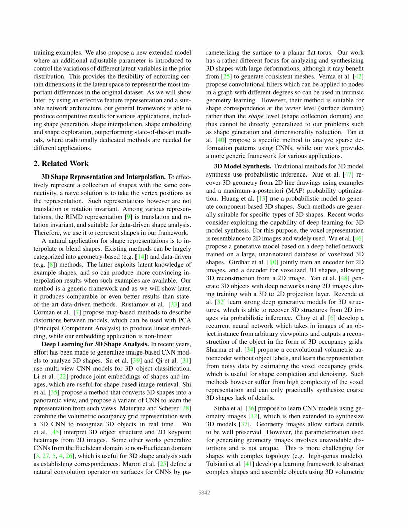
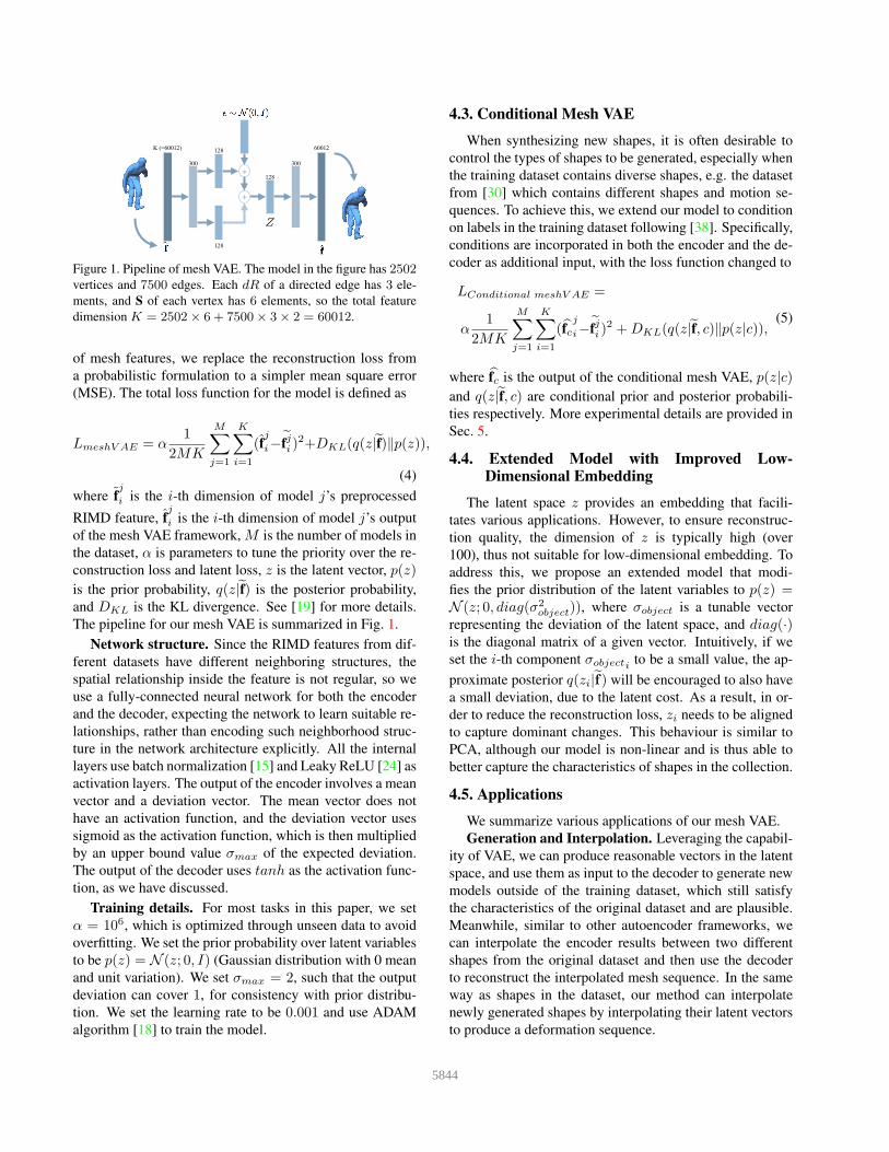
Figure 1. Pipeline of mesh VAE. The model in the figure has 2502

vertices and 7500 edges. Each dR of a directed edge has 3 ele-

ments, and S of each vertex has 6 elements, so the total feature

dimension K = 2502× 6 + 7500× 3× 2 = 60012.

of mesh features, we replace the reconstruction loss from

a probabilistic formulation to a simpler mean square error

(MSE). The total loss function for the model is defined as

LmeshV AE = α1

2MK

M∑

j=1

K∑

i=1

(fj

i−fji )

2+DKL(q(z |f)‖p(z)),

(4)

where fj

i is the i-th dimension of model j’s preprocessed

RIMD feature, fj

i is the i-th dimension of model j’s output

of the mesh VAE framework, M is the number of models in

the dataset, α is parameters to tune the priority over the re-

construction loss and latent loss, z is the latent vector, p(z)

is the prior probability, q(z |f) is the posterior probability,

and DKL is the KL divergence. See [19] for more details.

The pipeline for our mesh VAE is summarized in Fig. 1.

Network structure. Since the RIMD features from dif-

ferent datasets have different neighboring structures, the

spatial relationship inside the feature is not regular, so we

use a fully-connected neural network for both the encoder

and the decoder, expecting the network to learn suitable re-

lationships, rather than encoding such neighborhood struc-

ture in the network architecture explicitly. All the internal

layers use batch normalization [15] and Leaky ReLU [24] as

activation layers. The output of the encoder involves a mean

vector and a deviation vector. The mean vector does not

have an activation function, and the deviation vector uses

sigmoid as the activation function, which is then multiplied

by an upper bound value σmax of the expected deviation.

The output of the decoder uses tanh as the activation func-

tion, as we have discussed.

Training details. For most tasks in this paper, we set

α = 106, which is optimized through unseen data to avoid

overfitting. We set the prior probability over latent variables

to be p(z) = N (z; 0, I) (Gaussian distribution with 0 mean

and unit variation). We set σmax = 2, such that the output

deviation can cover 1, for consistency with prior distribu-

tion. We set the learning rate to be 0.001 and use ADAM

algorithm [18] to train the model.

4.3. Conditional Mesh VAE

When synthesizing new shapes, it is often desirable to

control the types of shapes to be generated, especially when

the training dataset contains diverse shapes, e.g. the dataset

from [30] which contains different shapes and motion se-

quences. To achieve this, we extend our model to condition

on labels in the training dataset following [38]. Specifically,

conditions are incorporated in both the encoder and the de-

coder as additional input, with the loss function changed to

LConditional meshV AE =

α1

2MK

M∑

j=1

K∑

i=1

(fcj

i−fji )

2 +DKL(q(z |f, c)‖p(z|c)),(5)

where fc is the output of the conditional mesh VAE, p(z|c)

and q(z |f, c) are conditional prior and posterior probabili-

ties respectively. More experimental details are provided in

Sec. 5.

4.4. Extended Model with Improved Low-Dimensional Embedding

The latent space z provides an embedding that facili-

tates various applications. However, to ensure reconstruc-

tion quality, the dimension of z is typically high (over

100), thus not suitable for low-dimensional embedding. To

address this, we propose an extended model that modi-

fies the prior distribution of the latent variables to p(z) =N (z; 0, diag(σ2

object)), where σobject is a tunable vector

representing the deviation of the latent space, and diag(·)is the diagonal matrix of a given vector. Intuitively, if we

set the i-th component σobjectito be a small value, the ap-

proximate posterior q(zi |f) will be encouraged to also have

a small deviation, due to the latent cost. As a result, in or-

der to reduce the reconstruction loss, zi needs to be aligned

to capture dominant changes. This behaviour is similar to

PCA, although our model is non-linear and is thus able to

better capture the characteristics of shapes in the collection.

4.5. Applications

We summarize various applications of our mesh VAE.

Generation and Interpolation. Leveraging the capabil-

ity of VAE, we can produce reasonable vectors in the latent

space, and use them as input to the decoder to generate new

models outside of the training dataset, which still satisfy

the characteristics of the original dataset and are plausible.

Meanwhile, similar to other autoencoder frameworks, we

can interpolate the encoder results between two different

shapes from the original dataset and then use the decoder

to reconstruct the interpolated mesh sequence. In the same

way as shapes in the dataset, our method can interpolate

newly generated shapes by interpolating their latent vectors

to produce a deformation sequence.

5844

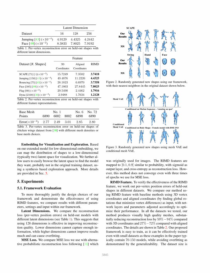
Latent Dimension

Dataset 16 128 256

Jumping [43] (×10−4) 4.9129 4.4325 4.2442Face [49] (×10−2) 8.3833 7.8025 7.9192

Table 1. Per-vertex reconstruction error on held-out shapes with

different latent dimensions.

Feature

Dataset [#. Shapes] 3D Aligned RIMD

Coordinates Coordinates

SCAPE [71] [1](×10−3) 15.7249 7.3582 3.7418

Jumping [150] [43] (×10−4) 49.4876 11.2226 4.4325

Bouncing [75] [43] (×10−4) 28.1823 6.6970 3.7358

Face [385] [49] (×10−2) 47.1863 27.8445 7.8025

Flag [90] (×10−3) 29.5490 2.4462 1.7916

Dyna [2168] [30] (×10−3) 2.9488 1.7634 1.2128

Table 2. Per-vertex reconstruction error on held-out shapes with

different feature representations.

Base Mesh No. 1 No. 6 No. 72Points 6890 6002 8002 6890 6890

Error(×10−4) 2.77 2.49 3.01 2.85 2.80

Table 3. Per-vertex reconstruction error on held-out shapes of

chicken wings dataset from [30] with different mesh densities or

base mesh choices.

Embedding for Visualization and Exploration. Based

on our extended model for low-dimensional embedding, we

can map the distribution of shapes to a low-dimensional

(typically two) latent space for visualization. We further al-

low users to easily browse the latent space to find the model

they want, probably not in the original training dataset, us-

ing a synthesis based exploration approach. More details

are provided in Sec. 5.

5. Experiments

5.1. Framework Evaluation

To more thoroughly justify the design choices of our

framework and demonstrate the effectiveness of using

RIMD features, we compare results with different param-

eters, settings and input within our framework.

Latent Dimensions. We compare the reconstruction

loss (per-vertex position errors) on held-out models with

different latent dimensions (see Table 1). This suggests that

using 128 dimensions is effective in improving reconstruc-

tion quality. Lower dimensions cannot capture enough in-

formation, while higher dimensions cannot improve results

much and can cause overfitting.

MSE Loss. We compare MSE loss we use with alterna-

tive probabilistic reconstruction loss following [11] which

Our

Results

NN

Our

Results

NN

Our

Results

NN

Our

Results

NN

SCAPE

Hand FaceSwing

Figure 2. Randomly generated new shapes using our framework,

with their nearest neighbors in the original dataset shown below.

Mesh VAE

Conditional

Mesh VAE Conditioned on Body Shape - Female model with BMI 29.8

Conditioned on Motion Sequence - ‘running on spot’

Figure 3. Randomly generated new shapes using mesh VAE and

conditional mesh VAE.

was originally used for images. The RIMD features are

mapped to [0.1, 0.9] similar to probability, with sigmoid as

output layer, and cross entropy as reconstruction loss. How-

ever, this method does not converge even with three times

of epochs we use for MSE loss.

RIMD Feature. To verify the effectiveness of the RIMD

feature, we work out per-vertex position errors of held-out

shapes in different datasets. We compare our method us-

ing RIMD feature with baseline methods using 3D vertex

coordinates and aligned coordinates (by finding global ro-

tations that minimize vertex differences) as input, with net-

work layers and parameters adjusted accordingly to opti-

mize their performance. In all the datasets we tested, our

method produces visually high quality meshes, substan-

tially reducing reconstruction loss by 59%−94% compared

with 3D coordinates and 27%−72% compared with aligned

coordinates. The details are shown in Table 2. Our proposed

framework is easy to train, as it can be effectively trained

even with small datasets as these examples in the paper typ-

ically contain 70-150 models, while avoiding overfitting as

demonstrated by the generalizability. The dataset size is

5845

Left Side Back

Linear

Interpolation

Data-Driven

Neural

Network

Neural

Network

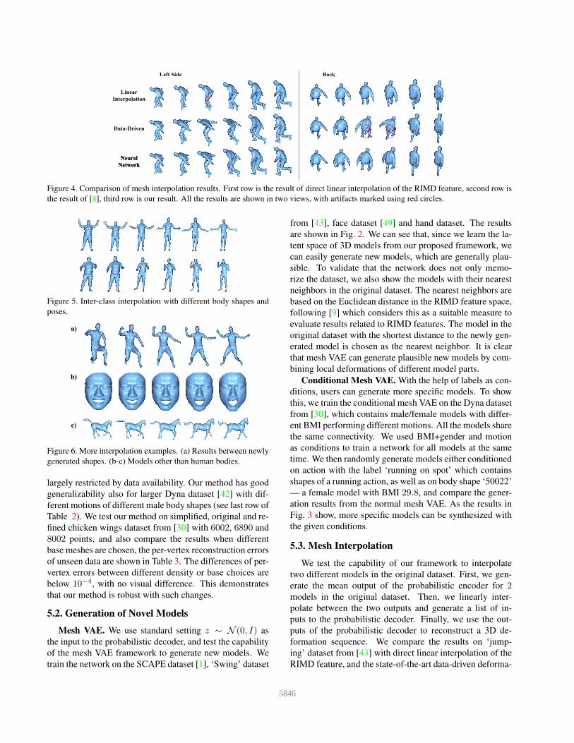
Figure 4. Comparison of mesh interpolation results. First row is the result of direct linear interpolation of the RIMD feature, second row is

the result of [8], third row is our result. All the results are shown in two views, with artifacts marked using red circles.

Figure 5. Inter-class interpolation with different body shapes and

poses.

a)

b)

c)

Figure 6. More interpolation examples. (a) Results between newly

generated shapes. (b-c) Models other than human bodies.

largely restricted by data availability. Our method has good

generalizability also for larger Dyna dataset [42] with dif-

ferent motions of different male body shapes (see last row of

Table 2). We test our method on simplified, original and re-

fined chicken wings dataset from [30] with 6002, 6890 and

8002 points, and also compare the results when different

base meshes are chosen, the per-vertex reconstruction errors

of unseen data are shown in Table 3. The differences of per-

vertex errors between different density or base choices are

below 10−4, with no visual difference. This demonstrates

that our method is robust with such changes.

5.2. Generation of Novel Models

Mesh VAE. We use standard setting z ∼ N (0, I) as

the input to the probabilistic decoder, and test the capability

of the mesh VAE framework to generate new models. We

train the network on the SCAPE dataset [1], ‘Swing’ dataset

from [43], face dataset [49] and hand dataset. The results

are shown in Fig. 2. We can see that, since we learn the la-

tent space of 3D models from our proposed framework, we

can easily generate new models, which are generally plau-

sible. To validate that the network does not only memo-

rize the dataset, we also show the models with their nearest

neighbors in the original dataset. The nearest neighbors are

based on the Euclidean distance in the RIMD feature space,

following [9] which considers this as a suitable measure to

evaluate results related to RIMD features. The model in the

original dataset with the shortest distance to the newly gen-

erated model is chosen as the nearest neighbor. It is clear

that mesh VAE can generate plausible new models by com-

bining local deformations of different model parts.

Conditional Mesh VAE. With the help of labels as con-

ditions, users can generate more specific models. To show

this, we train the conditional mesh VAE on the Dyna dataset

from [30], which contains male/female models with differ-

ent BMI performing different motions. All the models share

the same connectivity. We used BMI+gender and motion

as conditions to train a network for all models at the same

time. We then randomly generate models either conditioned

on action with the label ‘running on spot’ which contains

shapes of a running action, as well as on body shape ‘50022’

— a female model with BMI 29.8, and compare the gener-

ation results from the normal mesh VAE. As the results in

Fig. 3 show, more specific models can be synthesized with

the given conditions.

5.3. Mesh Interpolation

We test the capability of our framework to interpolate

two different models in the original dataset. First, we gen-

erate the mean output of the probabilistic encoder for 2models in the original dataset. Then, we linearly inter-

polate between the two outputs and generate a list of in-

puts to the probabilistic decoder. Finally, we use the out-

puts of the probabilistic decoder to reconstruct a 3D de-

formation sequence. We compare the results on ‘jump-

ing’ dataset from [43] with direct linear interpolation of the

RIMD feature, and the state-of-the-art data-driven deforma-

5846

First Dimension

Our Mesh VAE

Sec

on

d D

imen

sio

n

Sec

on

d D

imen

sio

n

First Dimension

PCA

Sec

on

d D

imen

sio

n

First Dimension

NPE

Sec

on

d D

imen

sio

n

First Dimension

t-SNE

Zoom In

Zoom In

Figure 7. 2D embedding of Dyna dataset. Different colors represent different body shapes. PCA embedding is very sparse so we include

two zoom-in subfigures as shown in the circles.

tion method [8], as shown in Fig. 4. We can see that direct

linear interpolation produces models with self-intersections.

Traditional geometry-based methods such as as-rigid-as-

possible interpolation [23] have similar problems (results

omitted due to space restriction). The interpolation result

in the latent space can avoid these problems. Meanwhile,

the data-driven method tends to follow the movement se-

quences from the original dataset which has similar start

and end states, and the results have some redundant mo-

tions such as the swing of right arm. Our interpolation re-

sult gives a reasonable motion sequence from start to end.

We also test inter-class interpolation on ‘jumping jacks’ and

‘punching’ datasets from [30], interpolating between mod-

els with different body shapes and poses. The results are

shown in Fig. 5. We show more interpolation results in

Fig. 6, including sequences between newly generated mod-

els and models beyond human bodies.

5.4. Embedding

As mentioned in Sec. 4, we adjust the deviation of la-

tent probability to let some dimensions of z capture more

important deformations. We utilize this capability to em-

bed shapes in a low-dimensional space. We use different

motion sequences of different body shapes from [30], and

compare the results of our method with standard dimension-

ality reduction methods PCA, NPE (Neighborhood Preserv-

ing Embedding) and t-SNE (t-Distributed Stochastic Neigh-

bor Embedding). When training meshVAE, we set the devi-

ation of the first two dimensions of the latent space z to be

0.1, and the remaining 1. The K-nearest neighbor setting for

NPE is set to k = 25 and the perplexity for t-SNE is set to

30, which are optimized to give more plausible results. The

comparative results are shown in Fig. 7. Since the dataset

contains a large number of diverse models, our embedding

is able to capture more than one major deformation patterns

in one dimension. When using the first two dimensions for

visualization, our method effectively divides all the models

according to their shapes, while allowing models of similar

poses to stay in close places. PCA is a linear model, and can

only represent one deformation pattern in each direction. In

this case, it can discriminate body shapes but the distribu-

tion is rather sparse. It also cannot capture other modes of

variation such as poses in 2D embedding. The results of t-

SNE have relatively large distances between primary clus-

ters, similar to PCA. This phenomenon is also mentioned

in [44]. NPE cannot even discriminate body shapes, which

shows the difficulty of the task. To quantitatively analyze

the performance of embeddings, we perform experiments

on the retrieval task using styles and poses as labels. The

AUC (area under the curve) values of the precision-recall

curves are: our method (0.5168) > t-SNE (0.4961) > PCA

(0.2272) > NPE (0.1391).

5.5. Synthesis based Exploration of the Shape Space

By adjusting the parameters σobject, our meshVAE

model is able to capture different importance levels of fea-

5847

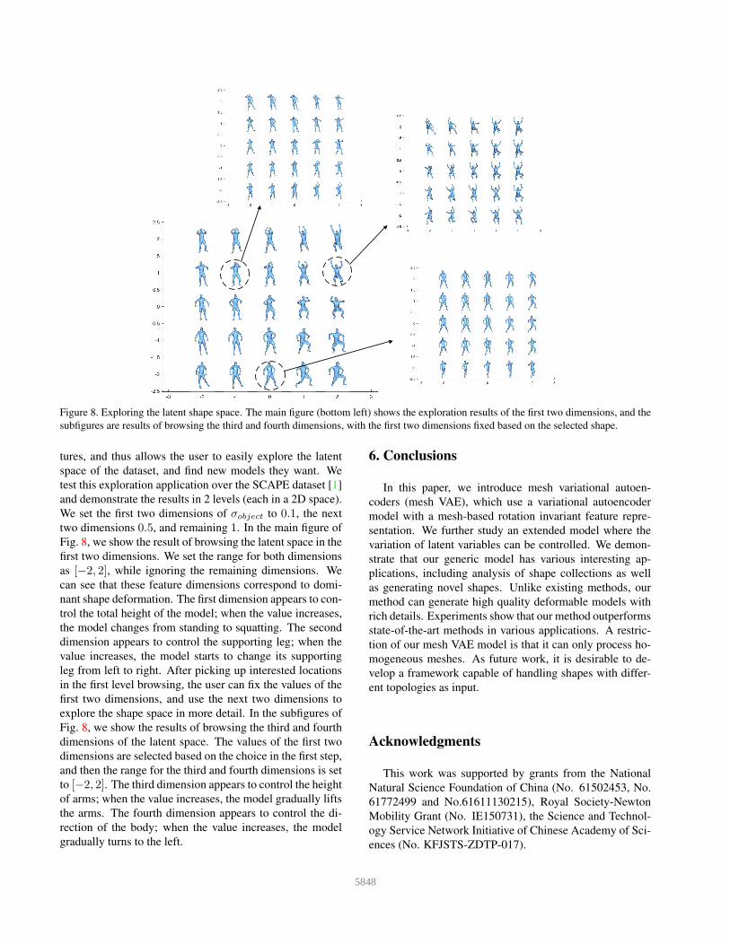
Figure 8. Exploring the latent shape space. The main figure (bottom left) shows the exploration results of the first two dimensions, and the

subfigures are results of browsing the third and fourth dimensions, with the first two dimensions fixed based on the selected shape.

tures, and thus allows the user to easily explore the latent

space of the dataset, and find new models they want. We

test this exploration application over the SCAPE dataset [1]

and demonstrate the results in 2 levels (each in a 2D space).

We set the first two dimensions of σobject to 0.1, the next

two dimensions 0.5, and remaining 1. In the main figure of

Fig. 8, we show the result of browsing the latent space in the

first two dimensions. We set the range for both dimensions

as [−2, 2], while ignoring the remaining dimensions. We

can see that these feature dimensions correspond to domi-

nant shape deformation. The first dimension appears to con-

trol the total height of the model; when the value increases,

the model changes from standing to squatting. The second

dimension appears to control the supporting leg; when the

value increases, the model starts to change its supporting

leg from left to right. After picking up interested locations

in the first level browsing, the user can fix the values of the

first two dimensions, and use the next two dimensions to

explore the shape space in more detail. In the subfigures of

Fig. 8, we show the results of browsing the third and fourth

dimensions of the latent space. The values of the first two

dimensions are selected based on the choice in the first step,

and then the range for the third and fourth dimensions is set

to [−2, 2]. The third dimension appears to control the height

of arms; when the value increases, the model gradually lifts

the arms. The fourth dimension appears to control the di-

rection of the body; when the value increases, the model

gradually turns to the left.

6. Conclusions

In this paper, we introduce mesh variational autoen-

coders (mesh VAE), which use a variational autoencoder

model with a mesh-based rotation invariant feature repre-

sentation. We further study an extended model where the

variation of latent variables can be controlled. We demon-

strate that our generic model has various interesting ap-

plications, including analysis of shape collections as well

as generating novel shapes. Unlike existing methods, our

method can generate high quality deformable models with

rich details. Experiments show that our method outperforms

state-of-the-art methods in various applications. A restric-

tion of our mesh VAE model is that it can only process ho-

mogeneous meshes. As future work, it is desirable to de-

velop a framework capable of handling shapes with differ-

ent topologies as input.

Acknowledgments

This work was supported by grants from the National

Natural Science Foundation of China (No. 61502453, No.

61772499 and No.61611130215), Royal Society-Newton

Mobility Grant (No. IE150731), the Science and Technol-

ogy Service Network Initiative of Chinese Academy of Sci-

ences (No. KFJSTS-ZDTP-017).

5848

References

[1] D. Anguelov, P. Srinivasan, D. Koller, S. Thrun, J. Rodgers,

and J. Davis. SCAPE: shape completion and animation of

people. ACM Trans. Graph., 24(3):408–416, 2005. 5, 6, 8

[2] F. Bogo, J. Romero, M. Loper, and M. J. Black. FAUST:

Dataset and evaluation for 3D mesh registration. In IEEE

CVPR, 2014. 1

[3] D. Boscaini, J. Masci, S. Melzi, M. M. Bronstein, U. Castel-

lani, and P. Vandergheynst. Learning class-specific descrip-

tors for deformable shapes using localized spectral convolu-

tional networks. Computer Graphics Forum, 34(5):13–23,

2015. 2

[4] D. Boscaini, J. Masci, E. Rodola, and M. Bronstein. Learn-

ing shape correspondence with anisotropic convolutional

neural networks. In Advances in Neural Information Pro-

cessing Systems, pages 3189–3197, 2016. 2

[5] D. Boscaini, J. Masci, E. Rodola, M. M. Bronstein, and

D. Cremers. Anisotropic diffusion descriptors. Computer

Graphics Forum, 35(2):431–441, 2016. 2

[6] C. B. Choy, D. Xu, J. Gwak, K. Chen, and S. Savarese. 3D-

R2N2: A unified approach for single and multi-view 3D ob-

ject reconstruction. In ECCV, pages 628–644, 2016. 2

[7] E. Corman, J. Solomon, M. Ben-Chen, L. Guibas, and

M. Ovsjanikov. Functional characterization of intrinsic and

extrinsic geometry. ACM Trans. Graph., 36(2):14:1–14:17,

2017. 2

[8] L. Gao, S.-Y. Chen, Y.-K. Lai, and S. Xia. Data-driven shape

interpolation and morphing editing. Computer Graphics Fo-

rum, 2016. 2, 6, 7

[9] L. Gao, Y.-K. Lai, D. Liang, S.-Y. Chen, and S. Xia. Effi-

cient and flexible deformation representation for data-driven

surface modeling. ACM Trans. Graph., 35(5):158:1–158:17,

2016. 1, 2, 3, 6

[10] R. Girdhar, D. Fouhey, M. Rodriguez, and A. Gupta. Learn-

ing a predictable and generative vector representation for ob-

jects. In ECCV, 2016. 2

[11] K. Gregor, I. Danihelka, A. Graves, D. Rezende, and

D. Wierstra. DRAW: A recurrent neural network for image

generation. In International Conference on Machine Learn-

ing, pages 1462–1471, 2015. 5

[12] X. Gu, S. Gortler, and H. Hoppe. Geometry images. In ACM

SIGGRAPH, pages 355–361, 2002. 2

[13] H. Huang, E. Kalogerakis, and B. Marlin. Analysis and syn-

thesis of 3D shape families via deep-learned generative mod-

els of surfaces. Computer Graphics Forum, 34(5):25–38,

2015. 2

[14] P. Huber, R. Perl, and M. Rumpf. Smooth interpolation of

key frames in a riemannian shell space. Computer Aided

Geometric Design, 52:313–328, 2017. 2

[15] S. Ioffe and C. Szegedy. Batch normalization: Accelerating

deep network training by reducing internal covariate shift. In

International Conference on Machine Learning, pages 448–

456, 2015. 4

[16] P. Isola, J.-Y. Zhu, T. Zhou, and A. A. Efros. Image-to-image

translation with conditional adversarial networks. In IEEE

CVPR, 2017. 3

[17] P. Kelly. Mechanics Lecture Notes Part III. Wiley, 2015. 3

[18] D. Kingma and J. Ba. ADAM: A method for stochastic opti-

mization. In ICLR, 2015. 4

[19] D. P. Kingma and M. Welling. Auto-encoding variational

Bayes. arXiv preprint arXiv:1312.6114, 2013. 1, 3, 4

[20] Z. Levi and C. Gotsman. Smooth rotation enhanced as-

rigid-as-possible mesh animation. IEEE Trans. Vis. Comput.

Graph., 21(2):264–277, 2015. 3

[21] J. Li, K. Xu, S. Chaudhuri, E. Yumer, H. Zhang, and

L. Guibas. GRASS: Generative recursive autoencoders for

shape structures. ACM Trans. Graph., 36(4), 2017. 3

[22] Y. Li, H. Su, C. R. Qi, N. Fish, D. Cohen-Or, and L. J.

Guibas. Joint embeddings of shapes and images via CNN

image purification. ACM Trans. Graph., 34(6):234, 2015. 2

[23] Y.-S. Liu, H.-B. Yan, and R. R. Martin. As-rigid-as-possible

surface morphing. Journal of Computer Science and Tech-

nology, 26(3):548–557, 2011. 7

[24] A. L. Maas, A. Y. Hannun, and A. Y. Ng. Rectifier nonlin-

earities improve neural network acoustic models. In Interna-

tional Conference on Machine Learning, volume 30, 2013.

4

[25] H. Maron, M. Galun, N. Aigerman, M. Trope, N. Dym,

E. Yumer, V. G. Kim, and Y. Lipman. Convolutional neural

networks on surfaces via seamless toric covers. ACM Trans.

Graph., 36(4):71:1–71:10, 2017. 2

[26] J. Masci, D. Boscaini, M. Bronstein, and P. Vandergheynst.

Geodesic convolutional neural networks on riemannian man-

ifolds. In IEEE ICCV Workshops, pages 37–45, 2015. 2

[27] J. Masci, D. Boscaini, M. Bronstein, and P. Vandergheynst.

ShapeNet: Convolutional neural networks on non-Euclidean

manifolds. arXiv preprint arXiv:1501.06297, 2015. 2

[28] D. Maturana and S. Scherer. Voxnet: a 3D convolutional neu-

ral network for real-time object recognition. In IEEE Con-

ference on Intelligent Robots and Systems, pages 922–928,

2015. 2

[29] C. Nash and C. K. Williams. The shape variational autoen-

coder: A deep generative model of part-segmented 3D ob-

jects. Computer Graphics Forum, 36(5):1–12, 2017. 3

[30] G. Pons-Moll, J. Romero, N. Mahmood, and M. J. Black.

Dyna: A model of dynamic human shape in motion. ACM

Trans. Graph., 34(4):120:1–120:14, 2015. 4, 5, 6, 7

[31] C. R. Qi, H. Su, M. Nießner, A. Dai, M. Yan, and L. J.

Guibas. Volumetric and multi-view cnns for object classifi-

cation on 3D data. In IEEE CVPR, pages 5648–5656, 2016.

2

[32] D. J. Rezende, S. A. Eslami, S. Mohamed, P. Battaglia,

M. Jaderberg, and N. Heess. Unsupervised learning of 3D

structure from images. In Advances in Neural Information

Processing Systems, pages 4997–5005, 2016. 2

[33] R. M. Rustamov, M. Ovsjanikov, O. Azencot, M. Ben-Chen,

F. Chazal, and L. Guibas. Map-based exploration of intrin-

sic shape differences and variability. ACM Trans. Graph.,

32(4):72:1–72:12, 2013. 2

[34] A. Sharma, O. Grau, and M. Fritz. VConv-DAE: Deep volu-

metric shape learning without object labels. In ECCV Work-

shops, pages 236–250, 2016. 2

5849

[35] B. Shi, S. Bai, Z. Zhou, and X. Bai. Deeppano: Deep

panoramic representation for 3-d shape recognition. IEEE

Signal Processing Letters, 22(12):2339–2343, 2015. 2

[36] A. Sinha, J. Bai, and K. Ramani. Deep learning 3D shape

surfaces using geometry images. In ECCV, pages 223–240,

2016. 2

[37] A. Sinha, A. Unmesh, Q. Huang, and K. Ramani. SurfNet:

Generating 3D shape surfaces using deep residual networks.

In IEEE CVPR, 2017. 1, 2

[38] K. Sohn, H. Lee, and X. Yan. Learning structured output

representation using deep conditional generative models. In

Advances in Neural Information Processing Systems, pages

3483–3491, 2015. 4

[39] H. Su, S. Maji, E. Kalogerakis, and E. Learned-Miller. Multi-

view convolutional neural networks for 3d shape recognition.

In IEEE ICCV, pages 945–953, 2015. 2

[40] Q. Tan, L. Gao, Y.-K. Lai, J. Yang, and S. Xia. Mesh-based

autoencoders for localized deformation component analysis.

CoRR, abs/1709.04304, 2017. 2

[41] S. Tulsiani, H. Su, L. J. Guibas, A. A. Efros, and J. Malik.

Learning shape abstractions by assembling volumetric prim-

itives. arXiv preprint arXiv:1612.00404, 2016. 2

[42] N. Verma, E. Boyer, and J. Verbeek. Dynamic filters in graph

convolutional networks. arXiv preprint arXiv:1706.05206,

2017. 2, 6

[43] D. Vlasic, I. Baran, W. Matusik, and J. Popovic. Articulated

mesh animation from multi-view silhouettes. ACM Trans.

Graph., 27(3):97:1–9, 2008. 5, 6

[44] M. Wattenberg, F. Viegas, and I. Johnson. How to use t-SNE

effectively. Distill, 2016. 7

[45] J. Wu, T. Xue, J. J. Lim, Y. Tian, J. B. Tenenbaum, A. Tor-

ralba, and W. T. Freeman. Single image 3D interpreter net-

work. In ECCV, pages 365–382, 2016. 2

[46] Z. Wu, S. Song, A. Khosla, F. Yu, L. Zhang, X. Tang, and

J. Xiao. 3D ShapeNets: A deep representation for volumetric

shapes. In IEEE CVPR, pages 1912–1920, 2015. 1, 2

[47] T. Xue, J. Liu, and X. Tang. Example-based 3D object re-

construction from line drawings. In IEEE CVPR, pages 302–

309, 2012. 2

[48] X. Yan, J. Yang, E. Yumer, Y. Guo, and H. Lee. Perspective

transformer nets: Learning single-view 3d object reconstruc-

tion without 3d supervision. In Advances in Neural Informa-

tion Processing Systems, pages 1696–1704, 2016. 2

[49] L. Zhang, N. Snavely, B. Curless, and S. M. Seitz. Spacetime

faces: High-resolution capture for modeling and animation.

In ACM SIGGRAPH, pages 548–558, 2004. 5, 6

5850