1

Introduction 1. Descriptive Statistics vs. Inferential Statistics 2. Terms

Variables - Take on different values

Measurement - Assign #’s

Qualitative Variables - Differ in kind Quantitative Variables - Differ in values

3. Scales of Measurement (Stevens, 1946)

Nominal Scales Ordinal Scales Interval Scales Ratio Scales

4. Exact Numbers vs. Approximate Numbers

Rounding is an issue for approximate numbers.

2

Research Problems The Sources of Problems Experience Deduction from Theory Related Literature The Research Problem Should 1. Advance existing knowledge. 2. Lead to new problems. 3. Be researchable. 4. Be suitable for you. 5. Be ethical. 6. Clarify exactly what is to be determined. 7. Be restricted in the scope. (Bad) ” What is the relationship between anxiety and achievement?” (Better) “Among high school students, is there a relationship between composite Stanford Achievement Test scores and Manifest Anxiety Scale scores?” (Bad) “Is it good to teach a foreign language in kindergarten?” (Better) “ What is the effect of foreign language education in kindergarten on the 3rd grade ITBS reading scores? “

3

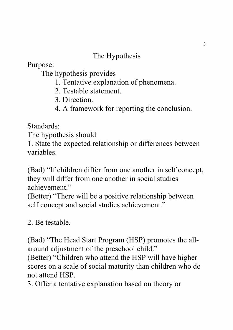
The Hypothesis Purpose: The hypothesis provides 1. Tentative explanation of phenomena. 2. Testable statement. 3. Direction. 4. A framework for reporting the conclusion. Standards: The hypothesis should 1. State the expected relationship or differences between variables.

(Bad) “If children differ from one another in self concept, they will differ from one another in social studies achievement.” (Better) “There will be a positive relationship between self concept and social studies achievement.” 2. Be testable. (Bad) “The Head Start Program (HSP) promotes the all-around adjustment of the preschool child.” (Better) “Children who attend the HSP will have higher scores on a scale of social maturity than children who do not attend HSP. 3. Offer a tentative explanation based on theory or

4

previous research. 4. Be concise. The Null Hypothesis Research hypotheses cannot be tested directly by available statistical procedures. H1: The end-of-year reading test scores are different for students taught by Method A and for those taught by Method B. H1: μA ≠ μB (μA - μB ≠ 0) H0: There is no difference in the end-of-year reading test scores between students taught by Method A and by Method B. H0: μA = μB (μA - μB = 0)

5

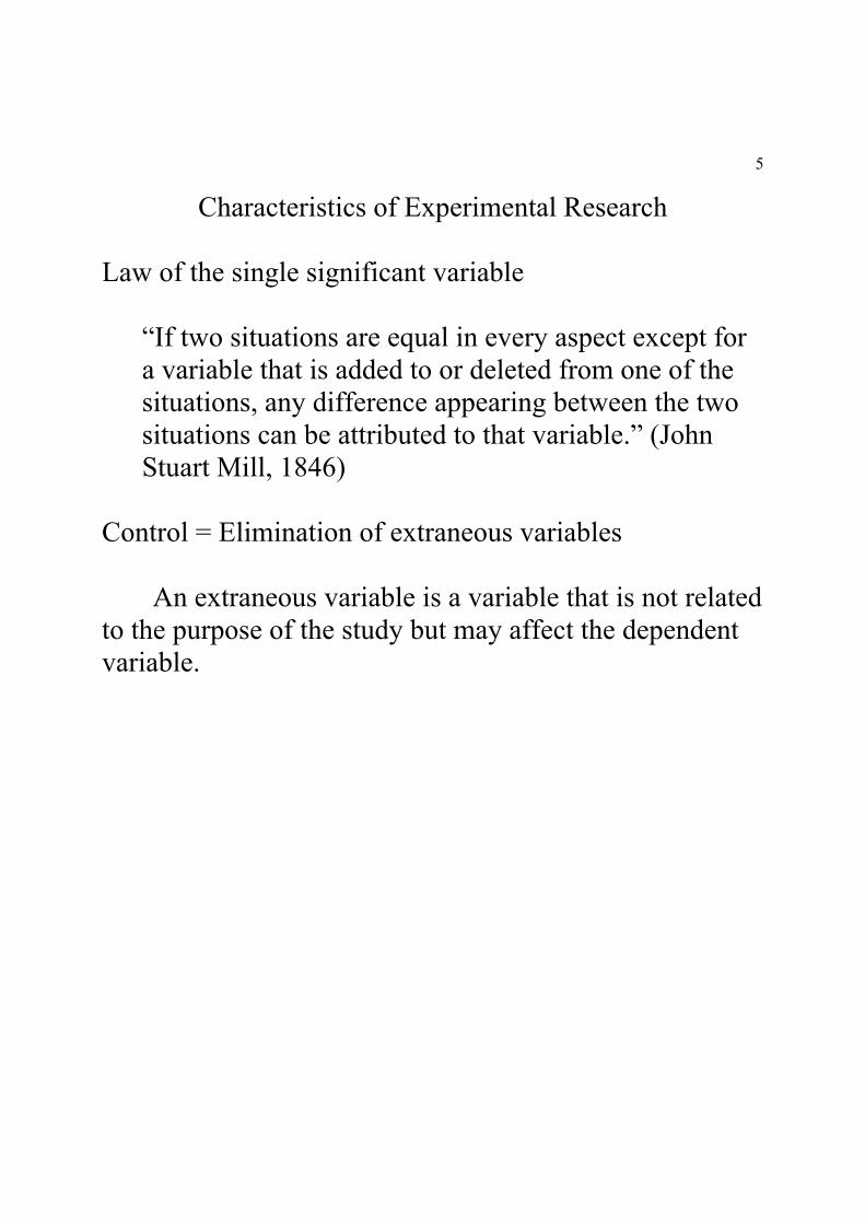
Characteristics of Experimental Research

Law of the single significant variable

“If two situations are equal in every aspect except for a variable that is added to or deleted from one of the situations, any difference appearing between the two situations can be attributed to that variable.” (John Stuart Mill, 1846)

Control = Elimination of extraneous variables An extraneous variable is a variable that is not related to the purpose of the study but may affect the dependent variable.

6

I. Controlling Inter-subject differences 1. Random Assignment

Every member of the population has an equal probability of being assigned to any of the groups.

2. Matching 3. Homogeneous Selection 4. Statistical Designs (ANCOVA, Repeated Measures) II. Controlling Situational Differences 1. Hold them constant.

2. Randomize the extraneous effect. 3. Add as another independent variable.

Control or Comparison Group

Experimental Group

7

Internal Validity (Definition) The degree to which extraneous variables are controlled in concluding or interpreting observed relationships. Campbell and Stanley (1963) have identified eight extraneous variables that frequently represent threats to the internal validity of a research design. 1. History: Incidents or events that occur during the research affect results. 2. Instrumentation (or Measuring instruments): Changes in the instruments affect the results. 3. Maturation: Maturational changes in subjects such as growing older or more tired, or becoming hungry, affect the results in quantitative research. 4. Pretesting: Taking a test can affect the results. 5. Regression (or statistical regression): There is a tendency for extreme scores to become closer to the mean score on a second testing. 6. Interaction of selection by maturation (or Selection-maturation interaction): 7. Selection (or Differential selection of subjects): Differences between groups of subjects affect results. 8. Mortality (or Experimental mortality attrition): Loss of subjects affects the results in quantitative research.

8

External Validity The effect to which results of a study can be generalized to other subjects, conditions, or situations I. Population External Validity The extent to which the results can be generalized to other people II. Ecological External Validity The extent to which the results can be generalized to other conditions Hawthorne Effect Relationship between Internal Validity and External Validity

Internal Validity

External Validity

9

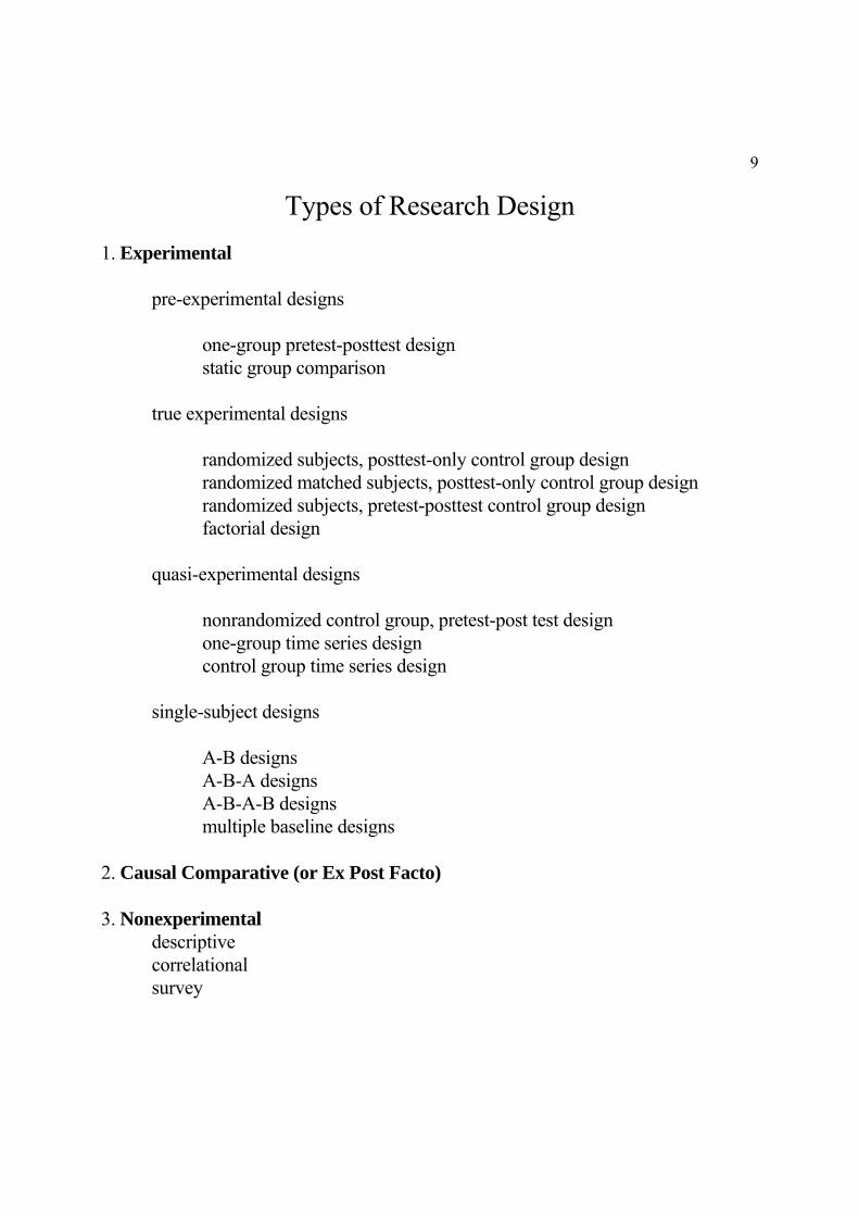
Types of Research Design 1. Experimental pre-experimental designs one-group pretest-posttest design static group comparison true experimental designs randomized subjects, posttest-only control group design randomized matched subjects, posttest-only control group design randomized subjects, pretest-posttest control group design factorial design quasi-experimental designs nonrandomized control group, pretest-post test design one-group time series design control group time series design single-subject designs A-B designs A-B-A designs A-B-A-B designs multiple baseline designs 2. Causal Comparative (or Ex Post Facto) 3. Nonexperimental descriptive correlational survey

10

Frequency Distributions

Organize Data Start with raw data. Then list.

Ungrouped-data frequency distribution Grouped-data frequency distribution

Grouped-Data Frequency Distribution

Minium’s Rules (2 - 6 for artistry) 1. Same i’s 2. Continuous intervals 3. Highest scores on top 4. 10 - 12 intervals (Others say 6 - 8) 5. Odd i 6. Lower score limits = multiple of the i

Steps for Construction

Other Issues

Relative Frequency Distribution (Proportion or %)

Exact Limits Cumulative Frequency and Cumulative % Percentile Scores and Percentile Ranks

11

Graphic Presentation Graphing qualitative data -- bar chart, pie chart Graphing quantitative data -- histogram, polygon Histogram

Labeling class interval

Scale Polygon

Comparison of two or more frequency distributions (Use relative frequency.)

Histogram and Frequency Curve

“The proportion of area under a frequency curve between any two score points is equal to the relative frequency of cases between these points.”

12

Characteristics of Frequency Distributions

Central Tendency

Variability

Shape

Normal Bimodal Skeweness (positive or negative)

Kurtosis (leptokurtic, platykurtic, mesokurtic)

13

Central Tendency and Variability

Data: ___________________ Class Test Scores ___________________ 1 8 10 10 10 12 2 1 5 10 15 19 3 0 2 12 18 18 ___________________ Q: What is the typical score in each class? (Central Tendency)

Mean, Median, Mode Q: How homogeneous is each class? (Variability)

Range, Variance, Standard Deviation

14

Mean Definition Formula Properties

1. Balance Point 2. Sampling Stability 3. Includes all the scores

(thus affected by extreme scores) Note Weighted vs. Unweighted Mean

Median

Definition 50th percentile rank Properties

1. Equal number of scores fall below or above. 2. Not so affected by extreme scores

Mode Definition Most frequently occurring number Properties

1. Used with variable on nominal scale. 2. Not stable 3. Easy

Central Tendency and Distribution Symmetry Which Measure of Central Tendency to Use?

15

Range Definition R = H - L Properties

1. Easy to calculate 2. Affected by extreme scores

Variance Definition Formula (Defining vs. Calculating) Properties

1. Includes all the scores 2. Stable 3. Not on the original scale

Standard Deviation (SD)

Definition Formula Properties

1. Includes all the scores 2. Stable 3. On the original scale

SD and the Normal Distribution Effect Size

16

Normal Curve History Properties of the Normal Curve

1. Symmetrical 2. Unimodal 3. Bell-Shaped 4. Asymptotic

Z Scores

Definition:

A standard score with mean = 0 and SD = 1 Formula:

Z Table

17

Z to Area Suppose mean = 100 and SD = 20

Problem 1: What proportion of cases fall below a score of 80?

Problem 2: Above 120? Problem 3: Above 80? Problem 4: Between the values of 90 and 120? Problem 5: Between the values of 110 and 120?

More Problems: Problem A: Below 85? Problem B: Between 98 and 116?

Area to Z

Problem 6: Find the score that separates the upper 20% of the cases from the lower 80%. Problem 7: Find the score that separates the lower 20% of the cases from the upper 80%. Problem 8: What are the limits within which the central 95% of scores fall?

More Problem: Problem C: Central 40%?

18

Standard Scores Example 1:

Psychology History

Score 85 90 Mean SD Z Example 2:

Test 1 Test 2 Score 65/100 70/100 Mean 50 50 SD Z Other Standard Scores

New Score = New SD (Z) + New Mean Percentile Ranks

19

Correlation

A. Definition Relationship between two variables

B. Strength C. Direction

Positive, Negative, or Zero D. Examples

1. Height and weight? 2. Age (6-12 yrs old) and time to run 50 yards? 3. Reading and math?

E. Scatterplot

20

Numerical Example ____________________ Name HT WT ____________________ George 72 160 Sam 66 144 Bill 68 154 Don 74 210 Jim 68 182 Ron 64 159 Chuck 63 200 Adam 73 198 Walt 61 132 Kyle 62 126 ____________________ Formula

21

Factors That Affect the Size of r 1. Linearity 2. Restriction of Range <<<<<<<<<<<<<<<NOTE>>>>>>>>>>>>>>>>>>>>> Correlation does not imply causation! Coefficient of Determination Spearman’s Rank Correlation (Rho) Coefficient

22

Simple Linear Regression

Correlation: Relationship between two variables, X and Y Regression: Predicting Y from X (or Explaining variation in Y from X) 1. Regression Equation (Regression Line) Y’ = a + bX or 0 1Y b b X= + 2. Prediction Errors (Standard Error of Estimate) 3. Coefficient of Determination (R-Square)

23

Probability An event (E) is a set of possible outcomes (O). P(E) = # of outcomes favorable to E / total # of possible O Probability Distribution

Example: Tossing the coin four times 1/16 4/16 6/16 4/16 1/16 p = .0625 p = .2500 p = .3750 p = .2500 p = .0625

HTTH THTH

HTTT HTHT THHH THTT TTHH HTHH TTHT THHT HHTH

TTTT TTTH HHTT HHHT HHHH _______________________________________________ 0 1 2 3 4 P(A or B) = P(A) + P(B) when A and B are mutually exclusive P(A and B) = P(A) X P(B) when A and B are independent

24

The Normal Curve as a Probability Distribution Example: Peabody Picture Vocabulary Test (PPVT)

Mean 100 SD 15 What is the probability of randomly selecting a PPVT score (i.e., ONE SCORE) of :

Problem 1: 115 or higher?

Problem 2: 91 or lower?

Problem 3: At least 30 points deviating from the mean?

Problem A: somewhere between 85 and 115?

25

Sampling Distribution Population ------- Sample

Parameter------ Statistic Sampling

Random Sampling Simple Random Sampling Stratified Sampling Cluster Sampling Systematic Sampling

Non-Random Sampling

Convenience Samples and Accessible Population Sampling Distributions of Means

Mean Standard Deviation (Standard Error of the Mean)

The Effect of the Sample Size (n)

26

Formula (a) Size of SE vs Size of SD (b) Effect of SD on SE (c) Effect of n on SE

Central Limit Theorem

1. Random sampling distribution of means tend toward a normal distribution irrespective of the shape of the distribution of X. 2. Larger n, closer to normal curve

27

Examples Assume Mean = 100 SD = 16 (Stanford-Binet IQ)

and n = 64 Problem 1: What is the probability of obtaining a sample mean IQ of 105 or higher? Problem 2: What is the probability of obtaining a sample mean IQ that differs from the population mean by 5 points or more? Problem 3: What sample mean IQ is so high that the probability is only .05 of obtaining one high or higher in random sampling? Problem 4: Within what limits would the central 95% of sample means fall? Problem A: Suppose now, mean = 250, SD = 50, (an achievement test) and n = 25

What is the probability of obtaining a sample mean score of 272 or higher?

28

One-Sample z Test (Hypothesis Testing)

Dr. Meyer’s Problem “Does home schooling make a difference - whether good or bad?” (How does the mean of the population of achievement scores for home-schooled fourth graders compare with the state value of 250?) Step 1: Specify the null and alternative hypotheses and set the level of significance. Step 2: Select the sample, calculate the necessary sample statistics. Step 3: Determine the critical values (or the p-value) . Step 4: Make the decision regarding the null hypothesis.

29

Some Issues: (a) Different Significance Levels (b) Type 1 vs. Type 2 Error (c) One-Tailed vs. Two-Tailed Tests (d) The p Value (e) Statistical vs. Practical Significance

30

Interval Estimation Point Estimate and Interval Estimate Back to Dr. Meyer’s Problem “What is the range of values within which I am 95% confident the population mean lies?” General Formula A 95% Confidence Interval

He is 95% confident that the population mean lies in somewhere between 252.4 and 291.6.

A 99% Confidence Interval

He is 95% confident that the population mean lies in somewhere between _____ and _____.

Compare and Contrast Hypothesis Testing vs. Interval Estimation

31

One-Sample t Test If the population standard deviation is known:

Conduct a z test If the population standard deviation is NOT known:

Conduct a t test Dr. Coffey’s Problem “Is the Internet use in her university more than or less than the national average of 6.75 hours per week?” The t Distribution

1. Family of Distributions (Degrees of Freedom) 2. When df is infinity, t = z 3. Mean = 0 4. Symmetric 5. Unimodal

32

Hypothesis Testing: Step 1: Specify the null and alternative hypotheses and set the level of significance. Step 2: Select the sample, calculate the necessary sample statistics. Step 3: Determine the critical values (or the p-value) . Step 4: Make the decision regarding the null hypothesis. Interval Estimation A 95% Confidence Interval

She is 95% confident that the population mean lies in somewhere between ____ and _____.

A 99% Confidence Interval

She is 95% confident that the population mean lies in somewhere between _____ and _____.

33

Independent t Test

Gregory’s Problem “Does the presence of a noticeable scent, both while reading a passage and later while recalling what had been read, affect the amount of information recalled?” Hypothesis Testing (Not Again!): Step 1: Specify the null and alternative hypotheses and set the level of significance. Step 2: Select the sample, calculate the necessary sample statistics. Step 3: Determine the critical values (or the p-value) . Step 4: Make the decision regarding the null hypothesis.

34

Interval Estimation A 95% Confidence Interval

He is 95% confident that the difference of the population means lies in somewhere between ____ and _____.

A 99% Confidence Interval

He is 95% confident that the difference of the population means lies in somewhere between _____ and _____.

Assumptions of the Independent t Test

1. Independence 2. Normality 3. Homoscedasticity

35

Dependent t Test When two groups are independent:

Conduct an independent t test When two groups are dependent:

Conduct a dependent t test Dr. Noname’s problem “Does an herbal treatment make a difference for attention deficit disorder (ADD) children?” Hypothesis Testing (Yes, the exactly the same steps again!): Step 1: Specify the null and alternative hypotheses and set the level of significance. Step 2: Select the sample, calculate the necessary sample statistics.

36

Step 3: Determine the critical values (or the p-value) . Step 4: Make the decision regarding the null hypothesis. Interval Estimation A 95% Confidence Interval

He is 95% confident that the difference of the population means lies in somewhere between ____ and _____.

A 99% Confidence Interval

He is 95% confident that the difference of the population means lies in somewhere between _____ and _____.

37

Hypothesis Testing for r

Dr. O’s Problem “Is there a relationship between the level of anxiety toward statistics and the performance of Quiz 1 in EPRS8530 class?” Hypothesis Testing (Yes, you must have memorized the steps by now!): Step 1: Specify the null and alternative hypotheses and set the level of significance. Step 2: Select the sample, calculate the necessary sample statistics. Step 3: Determine the critical values (or the p-value) . Step 4: Make the decision regarding the null hypothesis.

38

The Chi-Square Test

Used with data that consist of frequency Example: “Do differences exist in the proportion of registered voters preferring each prospective councilor?” Hypothesis Testing (Same steps again, of course.): Step 1: Specify the null and alternative hypotheses and set the level of significance. Step 2: Select the sample, calculate the necessary sample statistics. Step 3: Determine the critical values (or the p-value). Step 4: Make the decision regarding the null hypothesis.

39

One-Way Analysis of Variance (ANOVA)

Used when comparing 2+ means Alison’s Problem “Does the presence of a noticeable scent, both while reading a passage and later while recalling what had been read, affect the amount of information recalled? (A three-group design) Hypothesis Testing (Same steps again, of course.): Step 1: Specify the null and alternative hypotheses and set the level of significance. Step 2: Select the sample, calculate the necessary sample statistics. Step 3: Determine the critical values (or the p-value). Step 4: Make the decision regarding the null hypothesis. (Step 5: Conduct a post hoc test, if necessary.)