Valuing Flexibility - A Real Options Valuation of the...
79
Page 1 of 79 Valuing Flexibility - A Real Options Valuation of the Sisson Tungsten-Molybdenum Project Master Thesis MSc. Finance and International Business Author: Peter Spanner Madsen - Aarhus University, Business and Social Sciences Number of Characters and Pages: 130,175 characters & 79 pages Supervisor: Stefan Hirth, Department of Economics and Business April 2015
Transcript of Valuing Flexibility - A Real Options Valuation of the...

Page 1 of 79
Valuing Flexibility
- A Real Options Valuation of the Sisson
Tungsten-Molybdenum Project
Master Thesis
MSc. Finance and International Business
Author: Peter Spanner Madsen - Aarhus University, Business and Social Sciences
Number of Characters and Pages: 130,175 characters & 79 pages
Supervisor: Stefan Hirth, Department of Economics and Business
April 2015

Page 2 of 79
Abstract
The neoclassical capital budgeting process has been dominated by the DCF analysis, but
recently the real options framework has begun to win acclaim. This is due to the
inherent weaknesses of the DCF framework, which does not recognize uncertainty in
the variables employed in the valuation. As DCF valuation undervalues investment
opportunities under significant uncertainty, companies will underinvest and potentially
miss out on value creating opportunities. The thesis synthesises a real options
framework which recognizes uncertainty as well as the options available to an active
management. A case study approach is employed to illustrate a practical example of the
challenges of the real options analysis, in addition to highlighting the value derived
from the real options. The chosen case is a tungsten-molybdenum mining project in
Canada. The financial data of the project, as well as a comprehensive description of the
project was publicised as part of a Canadian securities regulatory filings. This formed
the basis of the financial data employed in the valuation. Two real options were
identified, the option to abandon the project, and the option to contract the output in the
case of unfavourable conditions. The options were valued separately and combined,
recognizing that the value of the separate real options is not the sum of the two options.
The value of the combined options to the management is estimated at 49.5 C$ Million
(M), an increase of 14.5% compared to the standard NPV value. The thesis concludes
by supporting the propositions made by the real options theory, substantiating the link
between uncertainty, management flexibility and the value of real options.

Page 3 of 79
Contents
1. Introduction............................................................................................................................... 5
1.1 Background & Problem Identification ................................................................................. 5
1.2 Case Study ........................................................................................................................... 7
1.3 Problem Statement ............................................................................................................. 7
1.3.1 Research Questions ...................................................................................................... 8
1.4 Real Options Literature Review ........................................................................................... 9
1.5 Real Options in Practice .................................................................................................... 11
1.6 Transitioning from Financial Options to Real Options ...................................................... 11
2. Theoretical Framework ........................................................................................................... 13
2.1 Valuation Framework ........................................................................................................ 13
2.2 Discounted Cash Flow ....................................................................................................... 14
2.2.1 Assumptions ............................................................................................................... 15
2.2.2 Three Inputs – Discount Rate, Free Cash Flow and Uncertainty ................................ 16
2.3 Simulation ......................................................................................................................... 18
2.4 Decision-tree Analysis ....................................................................................................... 21
2.5 Real Options Valuation ...................................................................................................... 22
2.5.1 When to use Real Options? ........................................................................................ 23
2.5.2 Types of Options......................................................................................................... 24
2.5.3 Determining the Value of an Option .......................................................................... 25
2.5.4 Analytical Approaches ................................................................................................ 27
2.5 Solution Techniques ...................................................................................................... 30
3. Case Study – The Sisson Tungsten-Molybdenum Project ....................................................... 36
3.1 Calculate NPV .................................................................................................................... 36
3.1.1 Assumptions Made in the NI-43-101 ......................................................................... 36
3.1.1.1 Reserves .................................................................................................................. 36
3.1.1.2 Production Capacity ................................................................................................ 37
3.1.2 Calculating the Dynamic Discounted NPV .................................................................. 38
3.1.2.1 Cost of Capital ......................................................................................................... 40
3.1.3 Sensitivity Analysis ..................................................................................................... 46
3.2 Analyse Uncertainty .......................................................................................................... 47
3.2.1 Exchange rate ............................................................................................................. 47
3.2.2 APT Price..................................................................................................................... 48
3.2.3 Modelling Uncertainty of APT Price ........................................................................... 50

Page 4 of 79
3.2.4 Modelling Uncertainty of the Exchange Rate ............................................................ 52
3.2.5 Correlation of Uncertainty Variables ......................................................................... 53
3.2.6 Volatility Estimate of the Underlying Asset ............................................................... 53
3.3 Event Tree ......................................................................................................................... 54
3.4 Create Decision Tree ......................................................................................................... 54
3.5 Estimate Value of Real Options ......................................................................................... 55
3.5.1 Abandonment Option with Changing Strikes ............................................................. 55
3.5.2 Option to Contract with Changing Strikes .................................................................. 56
3.5.3 Real Options Interactions and Non-additivity ............................................................ 57
3.5.4 Options Sensitivity Analysis ........................................................................................ 57
4. Conclusions.............................................................................................................................. 60
4.1 Main insights ..................................................................................................................... 60
4.2 Conclusion ......................................................................................................................... 60
4.3 Limitations and Further Research ..................................................................................... 61
5. References ............................................................................................................................... 63
6. List of Figures........................................................................................................................... 69
7. Appendix ................................................................................................................................. 70

Page 5 of 79
1. Introduction
1.1 Background & Problem Identification
According to Marshallian investment theory (Dixit & Pindyck 1994, p.260), companies
undertake investments to exploit temporary deviations from market-price equilibrium or
to exploit a competitive advantage. However, companies have always found it difficult
to value these investment opportunities. The capital budgeting process has a long
history, but advances in the field are rare. The dominating paradigm in the neoclassical
literature and dating back to the start of the eighties has been the net present value
(NPV) analysis. This is supported by a survey from 1978 which found that in 86% of
423 large companies employed NPV analysis (Schall, Sundem, and Geijsbeek, 1978).
Even before this, discounted cash flow (DCF) was a widely accepted valuation
technique, Segelod (1998) reports that the proportion of Furtune 500 companies using
DCF to value investments has steadily risen from 38% in 1962, 64% in 1977 to 90% in
1990-1993. A more recent study confirms this steady rise, as a survey by Graham and
Campbell (2002) shows that 74.9% of CFO’s in the survey always or almost always
used NPV as their capital budgeting.
However, academics and practicing managers are starting to recognize that NPV
analysis is an inadequate capital budgeting tool. The NPV analysis has several problems
in implementation of the analysis and in the assumptions behind the analysis. The NPV
analysis makes unrealistic assumptions in many cases, such as assuming expected cash
flows to be deterministic and presumes that once an investment decision has been made,
management has no operating flexibility. These kinds of assumptions can lead to
systematic undervaluation of projects as the value of operational flexibility is ignored,
e.g. the possibility to shut down a project (Hayes & Abernathy 1980). This systematic
undervaluation can lead to myopic decisions, underinvestment and a loss of competitive
position, since the companies are not able to properly quantify the value of operational
and strategic flexibility (Hayes and Garvin 1982).
The implementation by managers of the risk adjustment factor in the NPV analysis can
be problematic as the normal approach is to use a company’s weighted average cost of
capital (WACC), however, in practice managers often require hurdle rates much higher
than the cost of capital (Summers 1991, J.P. Morgan 2014), yet they still demand a
Page 6 of 79
positive NPV for projects. Dixit and Pindyck (1995) explain that this systematic
adjustment of the hurdle rate may be a result of managers realising that a company’s
options are valuable and keeping them open is often desirable.
So how should managers value projects that have operational flexibility?
Operational flexibility is potentially valuable when there is uncertainty regarding
expected cash flows and this uncertainty is resolved over time. As the uncertainty is
resolved, management may depart from the original operating strategy to accommodate
for this new information. The management may want to defer, expand, abandon,
contract, shut down or alter the operating strategy in other ways. These options
introduce asymmetry to the probability function of the NPV. This asymmetry makes it
possible to capture additional value available in favourable conditions or limit the
downside losses in unfavourable conditions. To value the options a new valuation
technique has to be employed that applies the expanded net present value criterion. The
sources of the expanded net present value is the traditional NPV (static or passive) of
cash flows plus the option value, which represent the operational flexibility (Trigeorgis
1998).
Expanded NPV (eNPV) = Static (Passive) NPV + Option Premium
The value of the option premium changes the way management should perceive risk.
The risk of the project is a positive factor when determining the value of the option.
This is in contrast to the NPV analysis, which increases the discount rate as the risk of
the project increases, thereby decreasing the NPV of a project. This means that there are
two opposite effects when calculating the real options value.
An investment opportunity in a mining project has been chosen for the case study as it
represents a clear example of the difficulties the traditional NPV approach will
encounter. O’Hara (1982) states that the actual return on investment can differ
substantially from the estimate of the feasibility study (a study determining the
economic viability of a mining project), this is because of errors in estimating capital
costs, ore reserves, operating costs, mineral revenue or operating productivity. This
problem can be alleviated by incorporating flexibility into the valuation to help
management control the errors (Mayer & Kazakidis 2007). To further substantiate the

Page 7 of 79
problem, Davis (1995) reports a discrepancy between the sum of discounted cash flows
in mining companies and its market price.
1.2 Case Study
The research structure applied in the thesis is a linear-analytic structure suggested for
thesis work by Yin (2014). Following this structure, the thesis is compiled as follows:
stating the problem being studied, review of relevant literature, moving on to the
theoretical methods applied, data input collected to be analysed, ending with the
findings, conclusions and implications for the issue being studied.
A case study can be defined in two parts as: “a case study investigates a contemporary
phenomenon (the “case”) in its real-world context, especially when the boundaries
between phenomenon and context may not be clearly evident”. The case is the Sisson
Project, which will be defined below. The second part is a definition of the case study
design and data collection methods (Yin 2014). This case study is designed as a single-
case study to determine whether the circumstances of the case and propositions stated
can be determined to be true or other explanations are more valid. This will enable me
to do a critical test of existing theory.
Case study research allows for a holistic and real-world perspective in the study of a
phenomenon such as capital budgeting processes. At the same time it allows me to do
an exploratory study, as shown in Allison & Zelikow (1999) who utilises a single case
study to form the basis of significant generalization (Cuban missile crises). However,
analytical generalizing of theoretical propositions can also be done by “multiple sets of
experiments that have replicated the same phenomenon under different conditions”. The
analytical technique applied is pattern matching, comparing predictions from theory
with data collected based on the findings of my case.
1.3 Problem Statement
The focus of the thesis is to analyse the valuation process of a natural resource
exploration (NRE) investment project in an uncertain environment to improve the
understanding of why it is necessary to recognize the value of options in corporate
investments. I will develop a framework for valuing options available to an active
management, which will enable managers to make more informed investment decisions

Page 8 of 79
in order to avoid systematic undervaluation and underinvestment of corporate
investment opportunities.
The thesis will apply an eNPV framework to estimate the value of the Sisson Project
when operational flexibility is included in the valuation. The value of the traditional
NPV analysis will be compared to that of the eNPV analysis. This will enable me to
determine if traditional capital budgeting techniques undervalues investment
opportunities with options available to an active management.
The problem statement necessary to uncover this value is:
- What is the expanded net present value of the Sisson Tungsten-Molybdenum
Project in an uncertain environment?
1.3.1 Research Questions
The research questions have been posted as a way of organizing the thesis to help
identify the appropriate research method. At the same time the research questions will
structure which theoretical methods to be analysed.
- Why is DCF methods insufficient? How can the eNPV framework remedy the
problems of other capital budgeting methods?
- How should a valuation of a tungsten mining project be carried out?
- Which solution methods is the most appropriate to be employed in the eNPV
valuation of the case study
- What is the DCF value of the project?
- Which real options are available to the management?
- What is the options and eNPV value of the Sisson project?
Defining the Case: The Sisson Tungsten-Molybdenum Project
The project plans to develop one of the largest undeveloped tungsten deposits in the
world into a long-life mine. The deposit is located in New Brunswick, Canada. The site
will be developed as an open pit mining operation. The location has access to
infrastructure with sea access to the north and south. In addition, it is located in a
mining jurisdiction with a long history of mining projects.

Page 9 of 79
Tungsten is essential in electrical applications, medical equipment and
telecommunications. Its hardness is similar to diamonds and has a very high heat
resistance, making it a crucial metal for cutting and drilling tools. Molybdenum can be
used for high-grade steel alloys to be used in the automotive-, construction-, electrical-
and other industries. Tungsten and molybdenum ore will be extracted and transported to
the primary crusher. The crushed ore will then go to the processing plant where
grinding, flotation, thickening and de-watering processes will be carried out to produce
tungsten (W) and molybdenum (Mo) concentrate. The tungsten concentrate will then be
moved to a value-added processing plant (APT plant), which will refine the tungsten
concentrate to Ammonium Paratungstate (APT). The APT and molybdenum
concentrate will be trucked out for shipping to North America, Europe, Asia and
Australia.
The Sisson Project is operated by Northcliff Resources ltd. (Northcliff). They are a
mineral development company associated with Hunter Dickinson Inc., which is a global
mining group. Northcliff is a company devoted solely to the Sisson Project. It trades on
the Toronto Stock Exchange (TSX) under the ticker symbol NCF. The Sisson Project is
owned by Northcliff, holding the controlling interest (88.5%) and Todd Corporation of
New Zealand holding an 11.5 % share, functioning as a financing partner. In addition,
the Todd Corporation owns 15 % of Northcliff.
A Project feasibility study was conducted, and in January 2013 Northcliff confirmed the
viability of the project. The Project is now waiting for approval of the Environmental
Impact Assessment (EIA) report, which was submitted in July 2013. They are focusing
on finalising the approval by mid 2015 which will allow for arrangement of funding and
construction commencement. Northcliff estimates that, pending approval of EIA, the
project could start construction in late 2015 with a construction period estimated to last
several years. Commercial production has been planned to start in 2018.
1.4 Real Options Literature Review
Real options valuation (ROV) applies financial option pricing theory to real world
investment valuation. Financial options pricing theory was developed by Black, Scholes
and Merton in 1973. They developed the Black-Scholes (B&S) model for valuing no-
dividend European options by constructing a replicating portfolio with the same cash
flows as the option, relying on no arbitrage to price the option (Damodaran 2002). Cox

Page 10 of 79
and Ross (1976) formalized their theory in a concept where securities are valued by
relying on risk-neutral valuation. This meant that if expected rates of return on the
underlying asset are risk-adjusted, the risk-adjusted cash flows can be discounted at the
risk-free rate (Brennan & Trigeorgis 2000). The implication of the breakthrough in
valuing financial options by constructing a replicating portfolio is clear, as evident by
the volume of trading on The Chicago Board Options Exchange (CBOE). It began
trading in 1973 and was the first public options exchange. In 1975 the traders on the
exchange was using the B&S model for pricing and hedging options positions (Merton
1998). In the most recent market report from 2013, the nominal dollar value traded on
CBOE was US$ 551.701.766.386 in put and call options (2013 Market Statistics).
The transition from financial options to real options was greatly influenced by Myers
(1977) as he suggested that corporate assets such as growth opportunities can be viewed
as call options where the real options value depends on the discretionary future
investments of the firm. The valuation of options was further advanced by Cox, Ross &
Rubinstein (1979) as they recognised that an option can be valued by a binomial
discrete-time approach making option valuation simpler and making it possible to value
American type options. In 1985 Brennan & Schwartz applied real options to determine
the optimal production policy in a natural resource investment project. Later Cortazar &
Casassus (1998) implemented real options valuation for a copper mine with the option
to expand production capacity, they found the real option value to be higher than the
NPV used by the case company. Cortazar et al. (2000) studied the option to defer
exploration investments in a copper mine and found that a significant part of the project
value was due to the options available to the management. Empirical research on real
options in mining is limited, although some important papers tests empirically how well
real options theory predicts reality. Moel & Tufano (2002) studies the opening and
closing decision of mining operations. Utilising a database of North American gold
mines from 1988-1997, they find that real options theory can explain the pattern of the
decision to open or shutdown a mining operation. Colwell, Henker & Ho (2002)
focused on the closure option of Australian gold mines in the period of 1992-1995.
They find the average and median closure option to be economically significant, they
do, however, add the caveat that the option values vary over a large range, leading to a
limited usefulness of real options to some individual mines.

Page 11 of 79
1.5 Real Options in Practice
In the mid-1990’s the interest in real options theory grew substantially. This began in
the oil and gas industries before moving into other industries such as management
consulting, where analysts began to use the framework for valuing investment
decisions. Real options theory has now become a mainstay in mainstream academic
finance texts and has won the attention of the industry (Borison 2005). However, there
are different interpretations of what constitute ‘real options’. For some firms real
options is applied as a conceptual tool for strategic planning, whereas others use it in the
in the more conventional form as a valuation technique (Triantis & Borison 2001).
Busby & Pitts (1997) asked all Finance Directors in FTSE 100 index whether they
recognized options in their businesses, which 50% of them did. Most of the identified
options were growth or abandonment options. 35% of respondents thought that options
were highly or extremely important in influencing investment decisions, however, more
than 75% of the respondents did not have procedures for handling real options
valuation. A later survey by Graham & Harvey (2001) conclude that about one third of
company CEOs in Fortune 1000 always or almost always value investments with real
options. Ryan & Ryan (2002) also surveyed CEOs in Fortune 1000 and found about 10-
15% utilised real options. Triantis (2005) suggests that this discrepancy may be down to
the different definitions of real options. I will show that there are pitfalls in real options
valuation as well as practical implementation difficulties, such as limited understanding
of real options by corporate managers. Further, assumptions are often violated in
practice, which may be some of the explanation why real options proponents have yet to
convince many companies of the value of real options theory.
1.6 Transitioning from Financial Options to Real Options
There are difficulties in the transition from financial options to real options, as Merton
(1998, p. 343) noted in a lecture for the Nobel Prize in Economics, in which he issued a
strong word of caution about the theoretical issues of using the financial options theory
for valuing real options. In his concluding remarks he states "the mathematics of
financial models can be applied precisely, but the models are not at all precise in their
application to the complex real world ... The models should be applied in practice only
tentatively, with careful assessment of their limitations in each application." Other
prominent authors within the field of real options are also weary of the complications
when trying to apply financial models to the real world. Copeland & Tufano (2004)

Page 12 of 79
states that two main differences between financial options and real options should be
considered before applying options theory to corporate investments: Firstly, it can be
problematic to estimate the value of the underlying asset, e.g. R&D of drugs has no
observable market price. However, when the underlying asset has a good proxy in the
market, the market can serve as a guiding point. Secondly, financial options and real
options differ in terms of how the options are defined. It can be unclear what a call real
option buys the caller, and how long it will last. E.g., when developing a new factory,
what is the maturity or how long does an option to expand last? - real options are not
always proprietary, which means a competitor may be able to erode the available
profits. Exercising a real option may also trigger the ability to exercise another option
(Trigeorgis 1996), e.g. building a new factory, could enable the management to expand
the factory in the future, which turns the option into a compound option, requiring a
different valuation method (Copeland & Tufano 2004). These examples show that real
options should not be treated like financial options, which can be valued relying on
market data to achieve a precise valuation. However real options can deliver a good
result when inputs are estimated thoroughly, and while it is not a precise measure, it can
function a way of quantifying the value of the option embedded in the project, to help
management in capital budgeting decisions.
Page 13 of 79
2. Theoretical Framework
In this section I will develop the theoretical framework to handle the valuation and
review the separate parts of the real options analysis to show why an eclectic framework
of previous attempts to quantify the value of flexibility will yield significant
improvements to the valuation framework.
2.1 Valuation Framework
The right valuation framework is dependent on the specific investment opportunity, as
the characteristics of an investment have significant impact on the appropriate valuation
method. Several different valuation methods try to extend the standard DCF framework
to incorporate the value of uncertainty and/or options (e.g. decision tree analysis and
simulation). I will show that these valuation techniques have their merits but also
shortcomings. This thorough review will highlight in which situations the methods are
applicable and in which they fail. The review will allow me to explain why the eNPV
framework is the only appropriate valuation method under significant uncertainty and
operational flexibility.
There are three basic valuation approaches for valuing an asset. The DCF valuation
values an asset based on the expected future cash flows this asset will generate. The
relative valuation uses the prices of other comparable assets to value the asset by
comparing variables that are common for both assets, like cash flows or book value.
Option pricing or contingent claims analysis values the asset by using option pricing
methods for assets, which has options characteristics (Damodaran 2006, p.9). DCF is
necessary for applying option pricing, therefore it is important to understand the
fundamentals of DCF (Damodaran 2002, p.12). Before reviewing the NPV model and
elaborating on why it is essential to the real options analysis, I will review the necessary
features of the valuation framework to be able to value the case project.
Trigeorgis (1996, p.52) states that “the presence of contingencies introduced by
managerial flexibility poses more serious problems, necessitating the use of option-
based valuation”.
I have summarized the most important problems and arguments for extending the
traditional NPV framework. Firstly, DCF techniques systematically undervalue
Page 14 of 79
investment opportunities (Copeland, Weston & Shastri 2004, p.308, Hayes &
Abernathy 1980, Hayes & Garvin 1982), as it fails to incorporate operating flexibility
(possibility to make or revise decisions at a future time) and the strategic option value of
a project (interdependence with future and follow-up investments) (Trigeorgis 1998).
Secondly, misapplication of DCF methods such as excessive risk adjustments in
projects with risk patterns that does not follow a random walk i.e. risk could decrease
with time (e.g. in a R&D project with different risk phases) (Hodder & Riggs
1985).This leads me to conclude that the appropriate valuation framework has to be able
to deal with uncertainty, operational flexibility and strategic options.
Although the NPV framework lacks the ability to value options, it is a fundamental part
of simulation techniques, decision-three analysis and real options valuation; therefore I
will review the NPV framework for application in the case valuation. Afterwards,
frameworks attempting to extend and improve upon the NPV analysis by dealing with
uncertainty, operational flexibility and/or strategic options will be reviewed for
applicability. At the same time I will show that the reviewed frameworks are a
complement to the real options analysis. The frameworks reviewed have been suggested
by decision scientists such as: Hertz 1979, Magee 1964, Trigeorgis & Mason 1987,
Kodukula & Papudesu 2006, Mun 2006, Amram & Kulatilaka 1999 and Copeland
2003.
2.2 Discounted Cash Flow
Firstly, I will, in short, review the basics of an NPV analysis. Secondly, I present the
assumptions underlying the NPV analyses to show why they are problematic in a stand-
alone analysis. Lastly, I will look at the application problems that both the real options
analysis and a stand-alone NPV analysis will have to deal with.
Mun (2006, p.63) states, “Value is defined as the single time-value discounted number
that is representative of all future net profitability”. To calculate this value, the NPV
method is the most widely applied method out of hundreds of DCF methods, that all
have a common goal of calculating the NPV of a project by discounting investment
costs and free cash flows by an appropriate discount rate. The calculated value is the
present value of all the project future cash flows less the investment costs (Kodukula &
Papudesu 2006, p.17). The NPV of an investment is an expression of the value to an
investor who has free access to capital markets, and should be compensated according
Page 15 of 79
to the equilibrium expected return on securities with equivalent risk (Myers 1987), or
put another way, risk should be perceived as the risk to the marginal (investor most
likely to be trading on the stock at any given point in time) well diversified investor in
the firm (Damodaran 2006, p.14, p.28).
2.2.1 Assumptions
The assumptions of an NPV analysis are not automatically fulfilled in a real world
scenario. Myers (1987) and Damodaran (2012) both state that DCF is a standard method
for valuing default-free zero coupon bonds, where discounting the bond at the risk-free
rate will find the present value of the bond. When moving away from this simple
valuation, the assumptions underlying the DCF will have to be reconsidered. This could
be going from valuing the default-free zero coupon bonds to valuing a corporate bond
where default risk is introduced. Moving on to investment projects where the expected
cash flows are assumed uncertain (Damodaran 2012, p.12, Myers 1987).
The assumptions of an NPV analysis assume either a reversible or an irreversible now
or never investment (Miller & Park 2002). If the cash flows are certain, then there is no
need for revising the investment, as the optimal investment strategy can be chosen from
the beginning and the assumptions hold true. This means that NPV method is good for
valuing investment projects which can be termed “cash cows” (projects held in a
projects portfolio for the cash generation and not for strategic value). At the same time,
this means that NPV is not suited for valuing businesses with growth opportunities or
R&D, as a significant component of their value is derived from the strategic option
value or management flexibility inherent in the investment. (Myers 1987, Trigeorgis
1999, p.1). If the investment is assumed reversible, which for many investments is
untrue, e.g. mining projects will not be able to recoup all capital expenses and would
incur a clean-up cost, the assumption of reversibility fails. If the investment is assumed
an irreversible now-or-never investment, the assumption breaks down for proprietary
investment projects, e.g. in mining projects where the land has been leased for a set
amount of time or bought, the investment decision may be delayed until the commodity
to be explored moves to a favourable price level (Dixit & Pindyck 1995). As shown, the
assumptions of the NPV analysis breaks down quite easily, highlighting the need for a
new expanded net present value framework.

Page 16 of 79
2.2.2 Three Inputs – Discount Rate, Free Cash Flow and Uncertainty
There are three inputs which determine the value of an NPV analysis. These will be
reviewed for applicability to the real options analysis.
2.2.2.1 Estimating the Discount Rate
The risk aspect of an investment project is notorious for being one of the most difficult
parts of the valuation to handle appropriately. The discount rate should be set at a level
which values the project according to the risk level. Risk is defined by Kodukula &
Papudesu (2006 p.35) as “...the variance of real outcomes around the expected
outcome”. When deciding the appropriate discount rate two factors are important to
consider. First, the magnitude of uncertainty of the cash flows. If there is no uncertainty,
the risk-free rate should be applied. Alternatively, if there is uncertainty, the type of risk
should be determined. There are two general types of risk, market risk and private risk.
Private risks are defined as risks not influenced by market fluctuations, (e.g.
technological success in R&D or geological risks inherent in mining projects estimate
of resource and reserves). Market risks are defined as risks which are driven by market
forces. Investment costs are usually considered private risk. Production phase free cash
flows are usually influenced by market risk because uncertainty (e.g. demand and price
fluctuations) is market driven (Mun 2006, p.68 & Kodukula & Papudesu 2006). If all
cash flow costs are discounted at the risk-adjusted rate, the costs will be too heavily
discounted, making the project appear more valuable than it really is (Mun 2006, p. 68).
Samis et al. (2004) describes this problem as using an all-use discount factor, which
leads projects with a high discount rate to depreciate the operating costs at a high level,
erroneously increasing the NPV of the project.
When the project has cash flows which are market driven, the discount rate for these
cash flows has to be set at a higher level than the risk free rate, as the risks of the cash
flows cannot be diversified, which means the owners are taking on a larger risk. The
discount rate the project should be commensurate with the risk level of the project. To
estimate the risk levels, the company will ideally try to find a proxy investment. This
proxy should have a similar risk profile as the project. If this is possible the returns of
the proxy will then be used as the discount rate for the project. The most common
method for quantifying the discount rate is to use the Capital Asset Pricing Model
(CAPM) (Damodaran 2012). The CAPM model states that the expected return of the
project should be the risk-free rate and a risk premium. The risk premium is calculated

Page 17 of 79
by the beta (measure of systematic undiversifiable risk relative to the capital markets)
times the difference of the market return and the risk free rate. If a proxy cannot be
found the WACC can be used and a premium can then be added if the project has a
higher than normal risk level (Kodukula & Papudesu 2006, p.43-44). WACC is a
commonly used method when the project is representative of the general risky nature of
the company’s activities (Mun 2006, p.69). When applying WACC the implicit
assumption is that companies adjust their debt levels to achieve a relatively constant
market-value leverage ratio, as reported in Copeland & Tufano (2004) companies will
typically not do this.
Other approaches which extends the CAPM model has been developed, although, these
multi factor models has failed in delivering significant improvement compared to the
default CAPM model. If CAPM is applied thoroughly it is still the most effective model
for dealing with risk (Damodaran 2006, p.35)
2.2.2.2 Estimating the Project’s Future Cash Flows
Free cash flows can be hard to predict, especially in projects where the lifetime is long,
as in the case project where the lifetime is projected to be 29 years. There are ways of
making the forecasts more reliable, e.g. econometric regressions, time-series analysis
and Monte Carlo simulation. Free cash flows are assumed predictable in NPV, but are
usually stochastic and risky in nature (Mun 2006, p. 67), as discussed in the previous
section this is problematic, since managers will have to reconsider their options if the
cash flows turn out differently than expected, which means the assumption of
predictable free cash flows break down when there is uncertainty over the free cash
flows. The real options approach (ROA) remedies the problem by assuming uncertainty,
and as well creating a strategy for the possible outcomes.
2.2.2.3 Dealing with Uncertainty
Typical approaches to modelling uncertainty will be to apply a sensitivity analysis to
assess which single uncertainty variable is the most influential. This will allow the
manager to assess how project NPV varies with each uncertainty variable. The manager
is then able to assess the projects economic viability under different market and
technical circumstances. However, sensitivity analysis is an inferior technique
compared to Monte Carlo simulation as this is an extended version of the sensitivity
analysis which considers the impact of all possible combinations (Trigeorgis 1996,

Page 18 of 79
p.54). Scenario analysis is able to gauge the overall level of uncertainty by recalculating
the free cash flows and NPV for different scenarios of the project. However, the
problem is how to choose between these scenarios (Amram & Kulatilaka, p.39-40
1999). Monte Carlo simulation will be used in the case study to create relevant
probabilities of cash flows to give a more detailed representation of the cash flows.
It is apparent that the standard NPV approach is problematic when valuing uncertain
cash flows over a long time horizon. Sensitivity analysis and scenario analysis can be
applied, but they fail in achieving a thorough estimation of the uncertainties of the
valuation. The eNPV approach will combine the NPV analysis with options based
valuation to overcome to inherent limitation of the NPV approach in dealing with
uncertainty. For modelling uncertainty, simulation has been suggested as a way of
improving the understanding of the variables and the probability function of NPV. In
the following section, I will review the basics of simulation and show why it is a crucial
part of a real options valuation.
2.3 Simulation
Before running a simulation, a deterministic NPV analysis is usually conducted and an
accompanying sensitivity analysis to identify the variables with the most impact on the
NPV. To show this graphically a Tornado chart will be applied. The most sensitive
variables are then chosen for a Monte Carlo simulation to be used in the dynamic NPV
analysis.
Simulation has a number of applications. Firstly, it can be used for modelling
uncertainty in an NPV framework. Secondly, it can be used to combine the variable’s
volatility into a single estimate of project volatility, which is necessary for conducting a
thorough real options analysis. Lastly, it can be utilised as a real option solution
technique. In this section I will focus on the characteristics of a dynamic NPV
simulation, application methods and problems in application. This will allow me to
show why simulation is not appropriate for a stand-alone valuation, but is useful in
combination with real options analysis.
Trigeorgis (1996) describes traditional simulation techniques as “repeated random
sampling from the probability distribution for each of the crucial primary variables
underlying the cash flows of a project...” The crucial primary variables are typically
Page 19 of 79
revenue, costs or other cash flow driving variables. This produces a probability
distribution of the NPV for a chosen management strategy. The management strategy is
put into the simulation as a mathematical model to simulate real-world settings where
the project uncertainty will be resolved over time, dependent on the pre-committed
operating strategy. Simulation is applied in an attempt to handle complex investment
decisions with uncertainty and enable management to handle input variables correlated
with each other. The variables stochastic process (e.g. Geometric Brownian Motion) has
to be predefined, and is determined by the characteristics of the variable(s) in the
simulation. Historical data or management judgement provides the source to determine
these characteristics. These variables may be correlated, if they are, this should be
determined and accounted for. Correlations between variables can be handled by
combining the variables into one combined single project volatility estimate.
Alternatively, if the variables are independent and expected to move in opposite
directions they can be kept separate to be able to distinguish the impact on value of the
separate variables. A rainbow type option allows for this, however, the option pricing
becomes much more complicated (Damodaran 2002).
Alternatively, methods for estimating the volatility includes; Logarithmic Cash Flow
Returns Method, Project Proxy Approach, Market Proxy Approach and Management
Assumption Approach. The Simulation Approach has been chosen for its ability to
include negative cash flows as well as being more accurate in asset analysis (Mun 2006,
p.190).
Monte Carlo simulation software such as Crystal Ball® is typically used for the
simulation. The software will generate an NPV value by simulating a value for each
input parameters from the assigned distribution. This is repeated a specified number of
times to generate the NPV probability distribution. The advantage of this method is its
ability to highlight the variability of input variables determining the NPV. It
acknowledges that the confidence of the accuracy of the single-point estimate of NPV,
traditionally supplied by a standard NPV analysis is often low. This is because
predicting the future in such a precise way is incredibly tough, if not impossible for
most investments (Mun 2006, p.104). Instead, Monte Carlo simulation estimates the
NPV probability distribution, to allow the management to get an estimate of the
probability that project NPV value is positive, and the probability of the ranges of value
the NPV can be within. As an example of how misleading a single best estimate can be,
Page 20 of 79
suppose a company makes a $1 million investment with three equally possible
outcomes, zero per year, $200,000 per year or $400,000 per year. This would come to a
best estimated return of $200,000 per year. However, if the company only has this
project, the company would go bankrupt if the project turns out to yield $0 per year, the
company would have a 1/3 chance of bankruptcy, even though the company’s best
estimate was $200,000 (Hertz 1979). This illustrates that even though an investment
may seem favourable, the dangers of high uncertainty has to be recognized.
Using Monte Carlo simulation for a dynamic NPV analysis can be problematic. Firstly,
as with any valuation, simulation is subject to the saying “garbage in, garbage out”. The
probability distribution of the variable inputs (e.g. cash flows, costs) has to be estimated
precise, otherwise the NPV probability distribution will be biased. Secondly, all the
interdependencies of the input variables can be very difficult to capture (Trigeorgis
1996). These two notions are true for simulation of project value and for using
simulation as an estimator of project volatility. Modelling NPV uncertainty by
simulation suffers from some of the same issues as a deterministic NPV analysis. I will
present the issues now and show why it is necessary to value the project by simulating
the probability distribution of the NPV as a way of modelling uncertainty to
complement real options theory.
Simulation is an extension of the traditional NPV analysis, and as such it is fallible to
the same assumptions underlying an NPV analysis. Simulation is applied in a forward
looking way as the management predetermines the strategy to be applied. This means
that Monte Carlo simulation does not allow for management flexibility if uncertainty is
resolved unexpectedly. The Monte Carlo simulation of the probability distribution of
NPV is not representative of a real world scenario with uncertainty, as managements in
the real world will have the ability to adapt their strategy to variables (e.g. cash flows)
which differs from expectations. The management might respond to unexpected cash
flows by abandoning, expanding or otherwise altering their operations strategy. This
means that simulation is better suited for projects which are predictable, such as path-
dependent or history-dependent projects (Trigeorgis 1996).
By applying simulation in the eNPV framework, the benefits of an improved
understanding of the NPV can be achieved and an aggregate volatility estimation can be

Page 21 of 79
produced. Using simulation complimentary to the real options analysis will help
overcome the main drawbacks of simulation.
2.4 Decision-tree Analysis
Decision-tree analysis (DTA) is also an extension of DCF, as it offers information about
future decisions under uncertainty and attempt to deal with the possible future decisions.
Decision trees can be used as a way of mapping graphically the strategic pathways a
company can undertake. This is done by “...mapping out all feasible alternative
managerial actions contingent on the possible states of nature in a hierarchical manner.”
(Trigeorgis 1996, p. 57). This method allows the management to analyse a large array of
complex sequential investment opportunities in an organized fashion. However, when a
lot of investment decisions branches into many decisions, the tree can become very
confusing. Trigeorgis (1996, p.66) refers to this problem as the decision-tree becoming
a decision-bush. The basic setup of the decision tree is a set of alternative decisions,
which are mapped by consequences of each decision dependent on a subjective
probability. Management then uses backwards induction to select the strategy where the
expected risk-adjusted NPV is maximized (Trigeorgis 1996). However, there are
problems in the application of decision tree analysis, especially in applying the correct
discount rate.
The expected value should optimally be calculated using risk-neutral probabilities (see
ROA section), as this would allow for the risk-free rate to be used for discounting.
Using risk-neutral probabilities in decision-tree analysis is erroneous for two reasons.
Firstly, the risk-neutral probabilities are calculated assuming a constant volatility. This
assumption is violated because the risk changes with each decision node, since the
decision will alter the project risk (e.g. shutting down a mine while mineral prices are
low). Secondly, risk-neutral probabilities require that the up and down jumps are
identical in size in the binomial lattice (two bifurcations/branches), to allow
recombining lattice. The jumps are not identical in size because the returns are not the
same for different branches in the decision tree. This requirement is known as the
Martingale process (knowledge of prior observed values does not change the
expectation of the next value). Because these requirements are not satisfied, the risk-
neutral probabilities are invalid. Since risk-neutral probabilities assumptions are
violated, the risk-free rate cannot be used as the discount rate ( Mun 2006, p.58).

Page 22 of 79
Applying DTA without the use of risk-neutral probabilities, but instead relying on
different discount rates at each decision nodes and at different time periods is a way to
solve this problem. Using different discount rates is necessary to account for changing
risks associated with the impact of decision nodes on project structure. Subjective
probabilities have to be applied at each node along with estimation of the appropriate
discount rate at each node. Estimation- and probability of occurrence errors will
compound and lead to incorrect valuations (Mun 2006, p.257). In conclusion, decision-
tree analysis does offer a good way of graphically representing the future decisions
available to the management, as decisions trees can be integrated into the real options
framework to map the contingent decisions where each node can be correctly valued by
a real options solution technique. It is however, on a stand-alone basis an economically
incorrect method because of the discount rate problem (Trigeorgis 1996, p.68). The real
options approach can solve this problem by incorporating the combined volatility from
Monte Carlo simulation to allow for risk-neutral valuation.
Having reviewed the alternative methods for handling investment opportunities with
uncertainty and management flexibility I can conclude they all suffer from problems
that can be remedied by applying simulation and decisions tree analysis in conjunction
with real options theory.
2.5 Real Options Valuation
A real option is any non-financial asset investment decision, be it to invest, divest,
expand or abandonment. The option gives the holder the right, but not obligation to
exercise the option at a predetermined price and time period. This is analogous to a call
or put option in the financial markets (Miller & Park 2002). Figure 1 illustrates how
financial- and real options are connected to each other.
Figure 1: Comparison of financial and real options, source: Felix Stellmaszek

Page 23 of 79
2.5.1 When to use Real Options?
Figure 2: when are options valuable, Source: Koller, et al. 2010
There are a number of prerequisites for applying real options analysis in a meaningful
way. Firstly, it should be possible to build a financial model where uncertainty factors
can be modelled and changed as new information arrives. Secondly, the management
should have flexibility, strategic options and be able to exercise the options as
uncertainty is resolved. Further, there has to be a significant uncertainty level regarding
the project cash flows, otherwise the optimal strategy could be chosen from the onset,
and the contingent decision would not be contingent on the outcome of the uncertainty.
Lastly, the management has to be willing, rational in exercising the options. In
companies where management and ownership is separated, principal-agent corporate
governance problems may come into play in these situations. This could be because a
manager’s remuneration is attached to how a specific investment fairs. The
manager/agent will then choose a course of action for the investment to gain maximum
economic benefit for him- or herself even though this could lead to a decrease in
shareholder value (Amram & Kulatilaka 1999, p.24, Mun 2006, p.135).
The real options framework is best suited for investments where the NPV value is either
modestly positive or slightly negative as this is where managers are forced to rely on
intuition to choose between foregoing an investment or investing. In these cases the real
options analysis can be conducted to supply management with the possibility to rely less
Page 24 of 79
on subjective intuition and more on the logic the option value offers to support or
discourage management intuition (Van Putten & MacMillan 2004).
2.5.2 Types of Options
As stated above, the management has to identify the options available and also the type
of option, as this is important when calculating the option value. There are a number of
generic option types, which are available to a mining operation (Haque, Topal & Lilford
2014).
2.5.2.1 Option to Abandon
The management can decide to create an abandonment option or it may already exist.
The real option analysis is able to enlighten the management about which circumstances
it is optimal to exercise the option. This is useful when deciding to abandon an
operating gold mine if prices decline, making exploration unprofitable. The
abandonment option is an option to sell for salvage value, which could include capital
expenditure and the cost of reclamation and closure. This is analogous to a put option in
the financial options terminology (Mun 2006, Copeland & Antikarov 2004).
2.5.2.2 Option to Expand
An option to expand could be the possibility to expand mining exploration capacity, e.g.
mining twice the amount of ore as usual, by investing additional capital to secure the
necessary surplus capacity for increasing output. This option is typically considered
when the commodity price increases, which can make the thus far non-economically
orebody economically viable because of the increased commodity price. An option to
expand is analogous to a call option.
2.5.2.3 Option to Contract
If a company is unsure of the market development, it might want to reduce its exposure
to the underlying by obtaining an option to contract operations by 50 percent at the time
the company deems it optimal within the next five years. This could be done by signing
a contract with a customer to buy some share of the output at a given price in the future
if the option is exercised. This is analogous to a financial put option.
2.5.2.4 Simultaneous Compound Options
This type of option is used when the value of one option depends on the value of
another option. Compound options were recognized by Black & Scholes in 1973, they

Page 25 of 79
found that the equity of a leveraged firm is actually a call option on the value of the
company, where the strike price is the face value of the debt. If a financial option is
written on the security of the firm, then a compound option is achieved. The option on
the security is then an option on the option on value of the firm. This is a simultaneous
compound option because the two options are active at the same time (Copeland &
Antikarov 2004). The assumptions underlying simultaneous compound options are that
both options occur at the same time and take an equal amount of time (Mun 2006).
2.5.2.5 Sequential Compound Options
In a sequential compound option the investment opportunity has multiple options over
several time phases, where the last option will depend on the success of the previous
option. Developing a factory could require multiple phases, which will depend on the
success of the previous phases.
2.5.2.6 Option to Change Strike Price and Volatility
Some options have changing strike prices or the volatility as time passes. For changing
parameters, it is extremely difficult mathematically to solve these options in a closed-
form model.
2.5.2.7 Option to Choose (Chooser Option)
When multiple mutually exclusive options exist, the management will have to choose
between different options. The combined value of the options are estimated by
incorporating all individual options into one option lattice, stepping backwards in time
by choosing the option which is most valuable at each decision node.
2.5.3 Determining the Value of an Option
2.5.3.1 Volatility (Risk) & Uncertainty
Before moving on to the determination of the value of an option, I will uncover the
difference between uncertainty and risk, as these two variables are sometimes used
interchangeably. However, they are not the same and should be defined, as they are both
important to the real options value.
Cash flows are a main value driver, however, cash flows are not certain in the real world
as cash flows are a forecast of the unknown to be resolved over time, events or actions.
Uncertainty can be thought of as the probability that a foreign exchange rate will be as
forecasted, or put another way the probability of an event occurring. The risk is the

Page 26 of 79
value change on a currency position (short/long) when the exchange rate moves. Mun
(2006) describes risk as “risk is something one bears and is the outcome of uncertainty”.
So if a company has perfectly hedged its exchange rate exposure, it will still be
uncertain about the movement of the exchange rate, but it will bear no risk.
In the real options framework risk is the volatility. The risk of a project is the “net
interaction of all uncertainties on cash flow” (Mun 2006). The risk is calculated using
the volatility of the rates of return. Uncertainty is needed to generate value in an option,
as it is the driver of the value. To be able to graphically show how uncertainty evolves
over time the cone of uncertainty has been developed.
Figure 3: Cone of uncertainty, source: Mun 2006, p.136
The model shows that uncertainty increases over time, which is not necessarily true for
risk. Logically, it makes sense that uncertainty increases over time as it is easier to
predict a project’s cash flows for a few months rather than for the next twenty years.
This is also depicted in the cone of uncertainty as it widens with time. This cone of
uncertainty actually looks like a binomial tree as this widens for every decision node. If
risk changes with time, the bounds of uncertainty become more complex and a
heteroskedastic (volatility changes over time) model for uncertainty need to be
developed. In real options, this is done by using non-recombining lattices.
Having defined the concept of volatility I will now move on to show what determines
the value of a real option. According to Copeland & Antikarov (2004) the value of a
real option depends on five basic variables with the possibility of more, depending on
the characteristic of the real option.

Page 27 of 79
The value of the underlying risky asset: The free cash flow from the project. When
the value of the asset underlying the real option increases, the value of the call option on
the real option increases as well (The opposite is true for a put option).
The exercise price: The exercise price can be seen as the investment cost to exercise
the option if the option is a call option (e.g. the option to expand operations by
increasing the output capacity of a mining operation). If the real option is a put option,
the exercise price is the amount received for exercising the option (e.g. abandoning a
project for salvage value). An increase in exercise price for a call option decreases the
call option value, whereas the value of a put option would increase.
The time to expiration of the option: The time to expiration increases the option
value when the time to expiration increases. This is true for both call and put options.
The standard deviation of the value of the underlying risky asset: The standard
deviation is a measure of the risky nature of the underlying asset. The value of a call
option depends on the value of the underlying exceeding the value of the exercise price.
When the standard deviation increases, the probability of the underlying asset exceeding
the exercise price also increases.
The risk-free rate of investment over the life of the option: The value of the option
increases when the risk-free rate increases.
Dividends: dividends usually belong to the world of financial options, but cash flow
lost to competition etc. can be seen as analogous to dividend in the real options world.
2.5.4 Analytical Approaches
Contradictory analytical approaches for application of real options analysis in practice
have been suggested by academics. It is important that the approach chosen for the real
options valuation is correct. The different approaches will yield different results
depending on the assumptions made in regards to calculating the underlying, what the
calculated value represents. Borison (2005) has analysed different approaches for three
fundamental issues, Applicability, Assumptions and Mechanics. I will review the
approaches and assess which approach is best suited to be applied in the case.
Page 28 of 79
2.5.4.1 The Classic Approach
The classic approach is the most direct application of option pricing theory to non-
financial asset valuation. The value derived from this approach represents financial
market value. This is the same as what the incremental investment would trade for in
the capital markets. The existence of a replicating portfolio from financial option
pricing theory is assumed. (portfolio of traded investments can be constructed to
replicate returns of the option, and the option can be valued based on no-arbitrage
argument). In addition, it is assumed that geometric brownian motion can describe the
asset price movement, which is also an assumption of the B&S model. The replicating
portfolio assumption for real options is lacking empirical evidence to validate that a
traded replicating portfolio of financial assets exists for a typical corporate investment
in real assets. Brealey and Myers (2000) explicitly say that replicating portfolio/no-
arbitrage cannot be used to justify application of real options.
2.5.4.2 The Subjective Approach
This approach uses subjective estimates of inputs instead of identifying a replicating
portfolio (still relies on the assumption that a replicating portfolio exists). The same
assumptions as the classic approach are assumed (the inputs of value of the replicating
portfolio follows a geometric brownian motion). DCF is suggested for determining the
current value of underlying asset. This is a subjective assessment as a proxy for traded
market values. The combination of the replicating portfolio (which is market based)
assumption and the use of subjective data (DCF) is inconsistent. The meaning of an
option value based on subjective DCF data with no-arbitrage assumption is unclear
(Borison 2005).
2.5.4.3 The MAD Approach
The marketed asset disclaimer (MAD) approach does not assume a traded replicating
portfolio, as with option pricing. Instead, the MAD approach assumes that using the
NPV value of the projects expected cash flows without flexibility can be used as an
estimate of the twin security known from the replicating portfolio. This is justified by
arguing that this assumption is not stronger than the assumptions behind the NPV (no-
arbitrage and market equilibrium), which is accepted and widely used. After the
underlying has been calculated the volatility is determined, and the binomial lattice
solution method can be applied.

Page 29 of 79
There is dissent among academics regarding the assumptions of the MAD approach.
Borison (2005) argues that there are differences in the traded twin security known from
DCF to that of option pricing. In DCF, a twin security refers to having the same beta, in
option pricing it refers to a security with the same returns in all states of the world. He
also criticises this approach for the use of subjective data for all input parameters except
cost of capital, which means that arbitrage opportunities may exist. In addition he
criticises Copeland & Antikarov’s (2004) assumption that the value of the underlying
follows a GBM walk which is attributed to Samuelsons Proof. He argues that this
argument is not necessarily true, as “there is no reason why a subjective assessment of
asset value must follow a random walk”. This topic is clearly subject to some
disagreement over the most appropriate method and assumptions to apply. However,
Copeland & Antikarov (2005) has answered this criticism by objecting to the statement
of subjective input parameters, as they clarify that a Monte Carlo simulation should be
used to model the uncertainty to calculate the volatility of the rate of return on the
project, thereby incorporating market data. The simulation can include input variables
correlated or uncorrelated with the market (i.e. public and private). In regards to the
stochastic nature of the input variables, they state that when modelling the inputs for the
cash flows they do not assume a GBM process. However, when estimating the volatility
of the rate of return of the project they argue that this follows a GBM process as
“changes in expectations are random, even though the expected cash flows have a
cyclical pattern” (e.g. mean-reversion in some commodities).
2.5.4.4 The Revised Classic Approach
This approach instructs that classic finance-based real options should be used where
investments are dominated by market-priced/public risks. Dynamic
programming/decision analysis should be used when investments are dominated by
private risks. The classic finance-based real options are interpreted just like with the
classic approach. For dynamic programming/decision analysis it is more complicated,
as the investment is dominated by private risks and subjective assessments are used to
evaluate risks.
Dixit & Pindyck (1994) explains this method as using contingent claims analysis
(option pricing) where the value of the asset is spanned by existing assets in the
economy (e.g. commodities traded on spot and/or future markets and goods that are
correlated with the values of shares or portfolios). When the value of the asset is not

Page 30 of 79
spanned, they suggest using dynamic programming/decision analysis. Amram &
Kulatilaka (1999) use the term ‘tracking’ instead of ‘spanned’ to make a similar
argument.
The primary difficulty in this approach is separating the investments in public or private
risks. After this, the approach suffers from the same problems as the classic approach
when risks are market driven. When risks are private in nature the problems of decision
analysis persists. For decision analysis it is a problem of getting correct subjective
inputs from experts.
2.5.4.5 The Integrated Approach
This approach separates the public and private risks like the revised classic approach,
however, this approach does not choose between an either public or privately dominated
investment, it determines which risks are public and which are private. Public risks are
assessed by identifying the replicating portfolio and applying no-arbitrage assumption
as in the classic approach. Private risks are assessed subjectively as in the revised
classic approach. The Integrated approach does not assume GBM. Borison (2005)
considers this approach to be more burdensome and difficult to explain to management,
however he also concludes that the integrated approach is based on the most accurate
and consistent theoretical and empirical foundation and should be applied where
quality and credibility is important (Borison 2005).
In the case study I will apply The MAD Approach described by Copeland & Antikarov
(2005), as this approach is the most intuitively appealing and it assumes no-arbitrage,
enabling the use of market data. It assumes that there is no perfectly correlated twin
security, but instead uses the NPV of the project without flexibility. The MAD approach
also allows me to estimate the volatility of the rate of return of the project by simulation
of changes in project value, thereby incorporating as much market information as
possible.
2.5 Solution Techniques
There are three general options valuation techniques for valuing real options: Partial
Differential Equations, Simulation and Lattices. Each of these techniques has different
solution methods applicable in different situations (Amram & Kulatilaka 1999,
Kodukula & Papudesu 2006). I will review the basics of these techniques, as well as the
limitations, assumptions, and applicability to the case. This will allow me to illustrate

Page 31 of 79
why the chosen method is applied and how other techniques could be useful in other
instances.
Figure 4: Real options solution techniques, source: Kodukula & Papudesu 2006
2.5.1 Partial Differential Equations
Partial differential equations (PDE) includes closed form solutions, where the most
widely known is the Black-Scholes equation. Other partial differential equations include
analytical approximation and numerical methods such as finite difference method. A
PDE can be defined as “an equation describing the changes in option values to changes
in the underlying asset value”. The option value is calculated by using the PDE and the
boundary conditions (equations describing decision rules and extreme values of the
option value). If possible, an analytical solution or closed-form solution like B&S can
then be calculated. However, option features such as multiple sources of uncertainty or
sequential options will make an analytical solution too complex (Amram & Kulatilaka
1999). If an analytical analysis is unfeasible, another solution method such as the
binomial model can be chosen, as this method can handle many types of real options. I
will only review the B&S model of the PDE’s as they can be very difficult to solve and
has many limitations which other methods can overcome (e.g. numerical methods can
typically only handle two sources of uncertainty) (Amram & Kulatilaka 1999, p.110).
Black & Scholes developed the first closed form equations, which assumes
deterministic exercise price of the real options:
B&S Equation: C = N(d1) S0 – N(d2) X exp(-rT)
C is the value of the call option, S0 is the current value of the underlying asset, X is the
cost of the investment or strike price, r is the risk-free rate, T is the time to expiration, d1

Page 32 of 79
equals [ln (S0/X) + (r + 0.5σ2)T]/T, d2 is equal to d1- σ √T, σ is the annual volatility of
the future cash flows of the underlying asset, and N(d1) and N(d2) are the values of the
standard normal distribution of d1 and d2 (Kodukula & Papudesu 2006). Copeland &
Antikarov (2004) lists seven assumptions of the B&S model. I have reviewed them and
explained why most of the assumption often is not met in a real corporate investment
project.
1. B&S assumes that the option to be valued is a European type option, however
most real options are possible to exercise early (e.g. abandoning a mine before
the resources are exhausted.
2. The option depends on only one source of uncertainty; the cash flows of a
natural resource investment will depend on more variables than the resource
market price, such as investment costs and operating costs.
3. The option depends solely on one underlying asset. This assumption rules out
valuing compound options such as staged construction.
4. No dividend; competition eroding profits can be seen as an analogy to dividends
5. Market price and stochastic process of the underlying are known; when the
market is liquid for the resource in questions this assumption can hold true.
However if the market is illiquid the market price can be unobservable.
6. The volatility is constant; the volatility may change as options are exercised, e.g.
if an option is exercised, it changes the riskiness of the project, the project
volatility will be changed.
7. Exercise price is known and constant; the price of an expansion will be an
estimate, which will often differ from the true cost.
As highlighted, the assumptions of the B&S model are very restrictive in a real options
setting, but other solution method will also require some of the assumptions to be
relaxed. Looking at real options methodologies applied in practice, the B&S model is
applied only sparingly, as the assumptions are generally not met. Further, the formula
does not reveal to the management how the option values are obtained, the term “black
box” has been used to describe the model’s lack of intuitive and explanatory features,
unlike the binomial lattice model (Triantis & Borison 2005).
Page 33 of 79
2.5.2 Monte Carlo Simulation
Monte Carlo simulation (MCS) can be used for valuing European options and American
type options. Boyle (1977) suggested valuing European options by simulating price
movements, thereby approximating a probability distribution of the option. The average
of the cash flow simulation is calculated and then discounted using the risk-free rate
(Gonzalo Cortazar 2000). Simulation for real option solutions are similar to the
technique for the NPV analysis described earlier. American and European options have
to be defined and valued by different approaches. European options can be valued using
methods for valuing cash flows determined by past information, as it is past-dependent.
As uncertainty is resolved, the option is valued by forward induction, which is only
possible when the present cash flows only depend on past events. When the cash flows
depend on the future information (e.g. American style options), forward induction is no
longer appropriate and backward induction has to be applied. (Gonzalo Cortazar 2000).
American type options have typically not been valued using simulation techniques since
each decision point will increase the computational requirements substantially, making
the simulation a very difficult task for even a modern computer (Kodukula & Papudesu
2006, Amram & Kulatiklaka 1999). Decision scientists have tried to modify MCS to be
able to handle American type options. Longstaff & Schwartz 2001 uses Least-Squared
Monte Carlo numerical method for solving American type real options, making it
possible for the simulation to handle multiple sources of uncertainty and path-dependent
cash flows (current value of cash flows depend on its history or path) (Amram &
Kudukilaka p.125, 1999). however, this method is more complex than other solution
methods such as lattices and has only recently been considered for American type
options (Lemelin, Sabour, Roulin 2006). This means that simulation is best suited for
European type options or for valuing path-dependent cash flows, as path-dependence
will increase the complexity of other solution methods as they will need to define state
variables that represent the path dependent information (Cortazar 2000).
2.5.3 Lattice Models
The last commonly used and suggested valuation technique involves using lattices.
Several different lattice solution methods exist, such as binomial, trinomial,
quadrinomial and multinomial. I will only review the binomial model as this is the most
commonly used and intuitively appealing. It also makes the analysis transparent as it
illustrates the future project values and the decision nodes, as well as being flexible in
Page 34 of 79
terms of handling input price and volatility changes. The binomial method is an
approximation of the B&S model, almost reaching the same result as B&S when the
number of time increments is increased enough.
The binomial lattice technique models uncertainty as a representation of the value of the
underlying asset evolution over time. When the underlying reaches a new time period
(the number of time period/increments can be freely chosen to achieve the desired level
of accuracy), the value of the underlying can either move up or down. This is
graphically illustrated in the binomial tree. The starting point is point S0, which is the
initial asset value. The asset value then moves either up or down, represented in the
binomial tree by the cone shape, Su as the up move and Sd as the down move. The factor
of up (u) and down (d) depends on the volatility of the underlying asset. The next time
period repeats this action, the tree widens like the possible values of the underlying
asset. This process continues until the time of expiration.
To solve the binomial lattice and calculate the option value, two approaches can be
chosen, either risk-neutral probabilities or a market-replicating portfolio. They are both
correct, however, the market-replicating portfolio is more difficult to understand and
apply (Mun 2006). I will only review the risk-neutral probability approach as this is the
approach I will apply in the case.
Risk-neutral probabilities rely on making cash flows risk neutral to be able to discount
cash flows (where risk has been accounted for) at the risk-free rate. This is in contrast to
the NPV approach where risky cash flows are discounted at the risk-adjusted rate. To
solve the binomial lattice using risk-neutral probabilities, the following inputs has to be
determined: value of underlying asset (S), exercise price (X), volatility of the natural
logarithm of the underlying free cash flow returns in percent (σ), time to expiration in
years (T), risk-free rate (rf) and dividend (b).
The next step is to calculate the up (u) and down (d) factors in the binomial lattice of the
underlying, calculated as: u = and d = = 1/u
Where is the time-step.
Using these calculations, starting from S0, multiplying the up and down factors by S0,
contintuing to the end of the binomial lattice of the underlying asset value.

Page 35 of 79
To perform a risk-neutral valuation of the option value, the risk-neutral probability has
to be determined. This is a mathematical term and has no economic or financial
meaning, calculated as:
P =
The risk neutral probability can then be applied in a backwards induction analysis to
determine the intermediate notes in the option value lattice going back to the present
time value of the option.
The intermediate note is determined by maximizing option value and the value of
keeping the option open, calculated as:
assuming continuous discounting approach (Mun 2006).
In practice the dominant solution methods are binomial/trinomial lattices, Monte Carlo
simulation and risk-adjusted decision trees. The solution method applied is generally
determined by the abilities of the analyst, time constrains and the nature of the project to
be valued (Triantis & Borison 2005). As described above the binomial model is suited
for handling multiple uncertainty as well as illustrating the option features, and for those
reasons, this is the solution method chosen for the case study.

Page 36 of 79
3. Case Study – The Sisson Tungsten-Molybdenum
Project
Figure 5: 5 step real options methodology, source: Copeland & Antikarov (2005)
For the estimation of the real options value in the case project, I will follow the
methodology outlined by Copeland & Antikarov (2005), which involves a five step
process to calculate the option value.
3.1 Calculate NPV
The data input for the static NPV has been sourced from the NI-43-101 Technical
Report on the Sisson Project. The report was commissioned by North Cliff Resources
ltd. Samuel Engineering, Inc., along with various other consulting firms) contributed to
the consolidated report (NI-43-101, p.25). Further information has been sourced to
analyse the price development factors.
I will now outline the assumptions made by the NI-43-101 report and the necessary
assumption made in the case study to calculate the real options value.
3.1.1 Assumptions Made in the NI-43-101
APT and Molybdenum price are US dollar denominated, necessitating exchange rate
assumptions. The NI-43-101 assumes an exchange rate of US/CAD 1:1 for capital costs.
For revenue estimation the exchange was calculated as 0.98-0.92:1 for the first four
years and 0.90:1 for year five and onwards. The post tax cash flow (not discounted) is
calculated in the NI-43-101 at C$ 1,837.644 M. The valuation is made from end of year
2012 quoted in Canadian dollars.
3.1.1.1 Reserves
When reporting about scientific and technical information concerning mineral projects
to the public in Canada, technical reports about exploration and other mining properties
are governed by the National Instrument 43-101 – Standards of disclosure for mineral

Page 37 of 79
projects (NI 43-101). Standard definitions are defined by the CIM Definition Standards
on Mineral Resources and Reserves (CIM Definition Standards)
CIM Standards are used for defining Mineral Resources and Mineral Reserves.
Mineral resources are a concentration of solid material of economic interest, with
reasonable prospects for eventual economic extraction. Mineral resources are sub-
divided into three groups listed in order of geological confidence; Inferred, Indicated
and Measured Mineral Resource. The Measured Mineral Resource can be converted
into Proven or Probable Mineral Reserve.
Mineral Reserves are the economically mineable part of the Measured and/or Indicated
Mineral Resource. Reserves are also sub-divided, being either Probable or Proven,
where Proven Mineral Reserve is attached with the highest geological confidence level
of the two. To qualify as a Probable or Proven Mineral Reserve it should be
demonstrated to be economic by at least a pre-feasibility study.
The Net Smelting Return cut-off grade (CoG) value is used to measure how much of the
Mineral Resource can be converted into Mineral Reserve (economically mineable
reserve). The CoG was compiled by including contributions from both Tungsten and
Molybdenum. The Value is based on metal prices, plant recovery factors, downstream
treatment, insurance, transportation losses and cost of sales parameters.
The Mineral Resources are estimated at 387 Mt (metric tons) at a NSR cut-off of 9 ($/t)
using both Indicated and Measured Mineral Resources. The Mineral Reserve ore above
CoG has been estimated at 334 Mt at a CoG of 8.83 ($/t) 1
3.1.1.2 Production Capacity
The head grades are the average grade of ore fed into the mill. The recovery is the
portion of metal contained in the ore that can be extracted by processing. These
assumptions determine how much Tungsten and Molybdenum can be extracted. The
annual average recovery is respectfully 77% and 82%.
The project will mill 281 million tonnes ore, with an average of 10.5 kt (thousand tons)
ore pa, to produce 15 M mtu of Tungsten Trixide (WO3) and 111.3 M lb (pound) of
Molybdenum (Mo)2
1 Appendix B
Page 38 of 79
3.1.2 Calculating the Dynamic Discounted NPV
The main value drivers will be analysed, and a probability distribution of NPV will be
estimated in the dynamic NPV valuation to analyse the effect of uncertainty on the NPV
estimate.
NPV = PV of free cash flow – PV of capital expenditure
PV of free cash flow =
,
PV of capital expenditure =
,
n= life of mine, r = risk free rate, = cash flow in period t,
The free cash flow, the capital expenditure as well as the cost of capital will now be
determined to calculate the discounted NPV of the project.
Free Cash Flow Assumptions
The Cash Flow Summary in the NI-43-101 report is grouped in different intervals of 1,
2 or 5 year intervals, therefore it was necessary to divide the cash flows into yearly
intervals. This was done assuming an equal cash flow for each year, i.e. the cash flows
grouped into 2 year intervals was split into yearly cash flows by allocating ½ to the first
year and ½ to the second year. In the production schedule3 it is visible that production
remains fairly stable in the groups, substantiating the assumption.
The project calculations are made from commencement of construction, which is noted
as year -2. The long term price of APT 350 US$ / mtu and a long term price of
Molybdenum (Mo) 15 US$ / lb has been utilised, which is based on the market study in
NI-43-101. The life of mine (LOM) production is estimated at 15 M mtu tungsten
(Wo3) and 111.3 M lb Molybdenum (Mo). Further, the exchange rate used for the
dynamic NPV is estimated using the cash flow summary provided in the NI-43-101
report, as the precise exchange rate assumptions was not provided.
The operating costs are determined by the total net smelter return (NSR) estimated at
491.4 C$ / mtu, which is the NSR of APT and Molybdenum combined. APT costs are
2 Appendix A
3 Appendix A

Page 39 of 79
calculated at 153.3 C$ / mtu. The costs of Molybdenum are incorporated in the APT
costs as by-product credits.
The project is subjected to three tax tiers; federal income tax, provincial income tax and
provincial mining tax under the New Brunswick Metallic Minerals Act (MMA). The
federal income tax in Canada is 15% on mining operations taxable income. The
provincial income tax in New Brunswick is 10%. The provincial mining tax is split in
two tiers, with a 2% royalty on “net income” and 16% tax on “net profits”. The LOM
income and mining taxes for the project is 893 C$ M.4 The Harmonized Sales Tax
(HST) has been excluded from the capital costs estimated as HST or parts of it can be
deferred or reclaimed.
The effective tax rate to be paid by over the life time of the project has been estimated
using the cash flow summary and used as the effective tax rate in the dynamic NPV
calculations.
Initial Capital Expenditure
As capital expenditure is uncorrelated with the market, it should be discounted at the
risk free rate. The capital expenditures estimates are considered to be accurate from
minus 5% to plus 15%. However, the capital expenditures will be included in the
sensitivity analysis for measurement of NPV by deviations from estimate in capital
expenditures.
Figure 6: Capital costs estimate, source: NI-43-101 Technical report
4 Appendix D

Page 40 of 79
Sustaining costs are split into Mining Equipment and Waste Management costs, the
total sustaining cost is estimated at 196 M C$ and are expenses for additional
construction costs and equipment purchases necessary during the operating phase, but
are not included in the regular operating costs.
Figure 7: Sustaining capital costs estimate, source: NI-43-101 Technical report
Capital expenditure in total 578.8 M C$ + 196 M C$ = 774,635 M C$
3.1.2.1 Cost of Capital
The cost of capital will be estimated by the WACC as explained in the NPV framework.
The WACC will be used for discounting the benefits of the project as they are market
driven, and the investment costs will be discounted at the risk free rate as the investment
costs are primarily private in nature and not correlated with the market. Northcliff is the
principal owner and developer of The Sisson Project. WACC is the cost of capital to the
firm, however, it can be applied as a proxy for project risk (Kudukula & Papudesu
2006). Northcliff’s cost of capital will therefore be applied as a proxy for estimation of
the cost of capital for the Sisson Project. The WACC of Northcliff is aligned with the
Sisson Project’s risk profile as Northcliff only has the Sisson Project in their Project
portfolio. Kudukula & Papadesu (2006) describes this as the project representing
“business as usual”.
Calculating WACC:

Page 41 of 79
Cost of Debt
Northcliff is a purely equity financed company which also means that the
part of the WACC equation drops out, leaving cost of equity as the cost of capital.
It should be mentioned that the WACC model assumes that the capital structure of the
firm is kept constant, which could alter the valuation if the company changes its capital
structure (e.g. by increasing debt the company would increase the value of the tax
shield).
Cost of Equity
Cost of equity is determined by the risk free rate, a market risk premium and the
company beta.
Expected return on Northcliff =
The expected return on an investment is the risk free rate plus a return to compensate for
the risk. The CAPM model estimates the extra return to compensate for the risk by
estimating the beta ( ) and the market risk premium, which is estimated by the expected
market return ( ) less the risk free rate ( ).
CAPM will be used to estimate the cost of equity for Northcliff.
Risk Free Rate ( )
When estimating the risk free rate, government default free bonds are normally used as
a proxy. The government bond to be applied should be determined using the currency of
which the cash flows are estimated, or it can be determined using currency
denomination of the cash flows (Koller et al. 2010). I will use the U.S Treasury bond as
the income of the project is US dollar denominated. To determine the appropriate time
period of the bond, I reviewed relevant literature: Bruner et al. (1998) surveyed large
firms and financial analysts who reported using the yields of 10 to 30 year bonds to
determine the risk-free rate. Damodaran (2012) recommends using a matching principle
where the duration of the default free bond is the same duration as the duration of the
cash flows, which is 27 years. However, the difference in U.S 10 and 30-year bond rates
has been less than 0.5% over the last 40 years (Damodaran 2008). At the same time
Page 42 of 79
Koller et al. (2010) argue that due to low liquidity in the 30-year Treasury bond, the
price and yield premiums might not reflect actual current value. Considering these
arguments I will apply the U.S 10-year Treasury bond rate as the risk free rate, in line
with Damodaran (2008) recommendations.
( ) = 1.76% ultimo 2012
Risk Premium ( )
The risk premium is usually estimated by observing the historical returns of a stock
market compared to the return on a default free security (risk-free rate) over a long time
period. When computing the average returns of the market securities and risk free rate,
some of the assumptions of the calculation are debated in regards to which yield the
most precise estimate. Three considerations are debated. These general considerations
include how to calculate the average returns, how long a time period should be used for
estimation and the choice of risk free rate. I apply a geometric average, as arithmetic
average returns would likely overstate the premium due to stock returns being
negatively correlated over time (Fama & French 1988). In regards to the time period
applied, Damodaran (2012) notes that the time period used to estimate the risk premium
can either be short term or long term. The argument for shorter time periods is that
investor risk aversion is likely to change over time. This makes shorter time periods
better for calculating a current estimate. However, this argument is offset by the need to
reduce the noise in the risk premium, as short term (10 or 20 years) time period standard
errors are likely to be as large as the estimated premium itself (Damodaran 2006). This
leads me to conclude that long time periods should be applied, which is in line with
Koller et al. (2010) who states the longest possible period should be used for estimating
risk premium. The risk free rate used has to be the same as applied in estimation of the
expected returns, and the same general considerations apply from when I chose the risk-
free rate. In addition, Koller et al. (2010) suggests using a 10-year government bond,
supporting the choice of U.S 10-year Treasury bond.
Damodaran (2015) has developed a historical premium using the S&P500 as the
historical earnings on the stock market, while the U.S Treasury 10-year constant
maturity bond has been applied as the risk-free rate.

Page 43 of 79
Figure 8: Historical risk premium, source: Damodaran homepage
Figure 8 shows the geometric average risk premium calculated using data from 1928 to
2012 to be 4.20%. However, there are problems with this approach. The risk aversion
issue as well as survivorship upward bias of risk premiums because of large samples
only being available with strong historical returns (Brown et al. 1995). Koller et al.
(2010) believes the market risk premium varies around 4.5% and 5.5% as none of the
risk premium models can estimate the premium precisely.
Figure 9: Geometric historical risk premium for different estimation periods, source: Damodaran (edited)
Figure 9 illustrates the impact of using different time periods in calculating the risk
premium.
Canada has a Aaa Moody rating, which is the same as The United States. No country
risk premium has been added in line with Damodaran (2015) published country risk
premium. The country risk premium is estimated by using Moody’s local currency
sovereign rating over the country bonds. This estimate is then compared to a default free
government bond rate.
Two other methods for estimating risk premium exists, survey premiums and the
Implied Equity risk Premium (forward looking premium).
Survey premiums are reported by large investment banks who report the expectations of
portfolio managers, however, these survey premiums are not widely used in practise as
they are highly volatile and are only short-term. A survey by Merrill Lynch in January
2012 of institutional investors globally reported their sentiment on risk premium, which
yielded a risk premium of 4.08% (Damodaran March 2014). Graham & Harvey (2013)

Page 44 of 79
surveyed CFO’s in the last six months of 2012 for their sentiment of a reasonable equity
risk premium (over the 10-year bond rate), they report an average of 3.83%. Fernandez
et al. (2011) compares the equity risk premium of analysts, companies and professors in
the U.S. Their results vary from 5% to 5.6%.
The implied equity risk premium takes into account the expected inflation and interest
rate increases, as opposed to the historical premiums. The implied equity risk premium
at the end of 2012 was reported at 5.78% calculated from expected return on stocks less
the risk-free rate (Damodaran March 2014). Collectively all these estimates give a range
of risk premiums of 3.83% to 5.78% from which to choose the historical market risk
premium. I follow the guidelines of Damodaran (2014a), who suggests for equity
premiums used to derive cost of capital, the historical premium is the most appropriate
as the cost of capital will determine the long-term investments of the firm.
( ) = 4.2%
Beta ( )
I will begin by estimating the raw beta using regression technique. This beta will be
improved upon by market comparables.
The raw beta regression:
To obtain the company beta, the stock return is regressed upon the market return to
produce a beta best fitting the regression. The stock return should include at least 60
data points. Monthly returns are better suited as more frequent data points will lead to
systematic bias due to returns in nontrading periods are regressed as zero (Damodaran
2012). The 60 data points monthly returns will add to five years worth of returns, which
has been tested and confirmed to be an appropriate measurement period (Alexander &
Chervany 1980). Some financial service companies like Bloomberg use two year
periods since the measurement period is a trade off between more data and the chance
that the company risk has shifted over the measurement period.
For Northcliff it was not possible to use five year data as the company has not been
trading over a five year period. I computed the beta for a two year weekly data-set
ending ultimo 2012. The market portfolio will have to be estimated using a proxy as it is

Page 45 of 79
unobservable. The split and dividend adjusted stock returns were regressed against the
adjusted S&P/TSX Composite Index returns, which represents the largest companies
listed on Toronto Stock Exchange, in line with Damodaran’s (2015a) method for
calculating beta of non-US stocks. The estimated beta was 0.315, which is very low.
This is an indication of low or-nontrading, as this will bias the beta downwards. The
standard deviation is also remarkably large at 0.611, which indicates that the beta could
be anywhere from -0.914 to 1.53 using two standard errors to estimate the beta with
95% confidence. The R2 of 0.003 suggests that the regression explains almost nothing
of the covariance of the stock and the market returns. The regression t-statistic of 0.63
indicates that the beta value cannot be rejected as different from zero. Because it was
not possible to estimate the company specific beta from historic returns, I will estimate
the industry average beta, then unlever the beta to account for financial risks. The
industry unlevered beta is suggested by Damodaran (2012) and Koller et al. (2010) as a
better beta estimate than the company specific beta.
To estimate the industry beta, I estimate each company’s beta, then unlever the beta
using company debt-to-equity.
Then the industry median unlevered beta is calculated by taking the median of the
sample companies (Koller et al. 2010).
Five companies have been identified for the calculation based on the geographical
location of mine sites, minerals produced and availability of market data to support a
five year 60 data point beta estimation regressed on the S&P/TSX Composite Index
returns.
When only a few comparable companies exist, a smoothing technique can be applied to
pull extreme observations towards the average. The technique is applied because of
Blume’s (1975) discovery of mean reversion in betas, reverting to the mean of all betas,
which is 1.
5 See Beta Calculation Excel Sheet for all data concerning beta

Page 46 of 79
Figure 10: List of companies and their respective unlevered beta and the median industry unlevered beta6
To validate this estimate I compared it to the U.S Metal and Mining Unlevered Industry
Beta pr. 01/01/13. In a sample of 77 companies, the beta was 1.54 (Damodaran 2015b).
Koller et al. (2010) argues for the use of a non-local index like the S&P500 as the
market portfolio, because the beta should be estimated according to the marginal
investor. To test the difference of the two indices I converted the S&P500 USD price to
CAD in each period. The adjusted median industry unlevered beta, ceteris paribus, was
estimated at 1.035. The regression results are quite similar, although the standard errors
using S&P 500 was a bit lower and the company General Moly, Inc’s beta became
insignificant.
In the CAPM calculation I will rely on the adjusted median industry unlevered beta
regressed upon the S&P/TSX composite index returns equalling: 1.43.
Cost of Capital Northcliff Resources ltd. =
7
3.1.3 Sensitivity Analysis
To estimate which variables the NPV is most sensitive towards I have conducted a
sensitivity analysis. Five variables were indentified in the NE-43-101 technical as
6 See Beta Calculation Excel Sheet
7 See Option Value Excel Sheet

Page 47 of 79
variables with potential to alter the value of the project. These five variables have been
adjusted by a 10% increase and a 10% decrease to inspect the value change in NPV.
Figure 11: NPV sensitivity analysis
Two variables have been chosen for further analysis, as they are the two most influential
variables. Copeland & Antikarov (2004) argue it is best to limit the number of variables
included and point to the fact that most volatility can be captured in two or three
variables. The variables identified as most influential are the exchange rate USD/CAD
and the price of APT. These two variables will be analysed and the stochastic processes
will be identified to be able to conduct a Monte Carlo simulation. This will enhance the
understanding of the variables interaction with each other as well as provide the
volatility estimate of the underlying asset required in the real options analysis. Applying
a Monte Carlo simulation for estimating volatility will give the most information
regarding the volatility of the underlying asset. The amount of recoverable ore was left
out of the sensitivity analysis, as this variable relies on geological data and specialist
knowledge regarding the uncertainty of the estimates in the NI-43-101 technical report.
3.2 Analyse Uncertainty
3.2.1 Exchange rate
3.2.1.1 Overview and Price Determinants
The USD/CAD exchange rate is ruled by the market, as it is a free floating currency.
The relationship between the USD and the CAD has historically been dominated by the
USD as the stronger currency. In 2012 the exchange rate level was close to parity,
however, the Sisson Project technical report assumes it moves towards the historical
-300000 -200000 -100000 0 100000 200000 300000
exchange rate usd/cdn
apt price
operating costs
capital expenditure
molybdenum price
10% increase
10% decrease

Page 48 of 79
rates. The long-term price level assumptions have been discussed in the NPV analysis.
The long-term price used in the options valuation is set at the same level used by the NI-
43-101 technical report. Samis et al. (2010) argues that the price expectations in the
options valuation should be consistent with the NPV calculations. This is also an
integral part of the comparison basis of the NPV value and the eNPV value.
3.2.2 APT Price
3.2.2.1 Industry Overview and Price Determinants
Tungsten (APT) is considered the universal industry price benchmark (Tungsten Sector
Report). The price is dependent on demand, supply and economic growth. APT is
typically priced in $/mtu (metric ton unit). 1 mtu is equal to 10kg, and 1 mtu of APT
contains 10kg of WO3. (ITIA – Pricing)
Tungsten (W) ore is separated from the ore to produce Ammonium Paratungstate
(APT). APT is an intermediate that can be used to produce Tungsten Trioxide (WO3),
by either thermal decomposition or chemical conversion. WO3 is then ready to be fused
into the desired application.
The demand for tungsten is principally driven by cemented carbide, which is used for
composite materials in oil and gas, power, mining and the automotive industry. This
accounted for 60% of total tungsten demand in 2013. Tungsten has a number of other
uses, where steel alloys are the most important as this makes up 24% of the total
demand.
Figure 12: Tungsten consumption by product, source: Tungsten Sector report
The level of global demand for tungsten has seen a rapid rise, evident by demand almost
doubling from 2000 to 2013, resulting in a demand of 93 kt of Tungsten. This demand

Page 49 of 79
is driven by a large consumption in China (48% of global consumption in 2013). North
America and Europe are the two other main consumers of tungsten with 38% of global
consumption in 2013.
Figure 13: World tungsten demand by region, source: tungsten sector report
The supply of tungsten relies heavily on China as they produce 80% (66.5 kt) of global
tungsten supply in 2013 (Tungsten Sector Report). Canada, Vietnam, Austria and
Portugal are the most important producers outside China (Tungsten Market Summary).
Scrap recycling is becoming a bigger factor in supply, with about 50% of North
American and European consumption supported by scrap recycling. How much scrap
will be recycled will depend on the price level as this determines the profitability scrap
recovery.
Tungsten prices were very low during the 1980’s and 90’s because China was
oversupplying the market, however, at the start of the new millennium China moved to
control tungsten production and export, as they recognized tungsten as a strategic
mineral. They introduced limits on tungsten extraction and export quotas, which forced
the price upwards after the initial build-up stockpile of tungsten had been absorbed by
the market. APT demand is highly correlated with the economic growth, which lead to a
rising APT price at the end of 2005 as the emerging economies experience accelerated
growth (Tungsten Sector Report, p. 11). The rising prices in 2010 are believed to be
caused by China introducing export quotas. The downward trend experienced at the
moment is believed to be caused by the slowing economic growth in emerging markets
and Europe, as well as China being expected to lift the export quotas due to a World
Trade Organization ruling (EU Commission Memo).
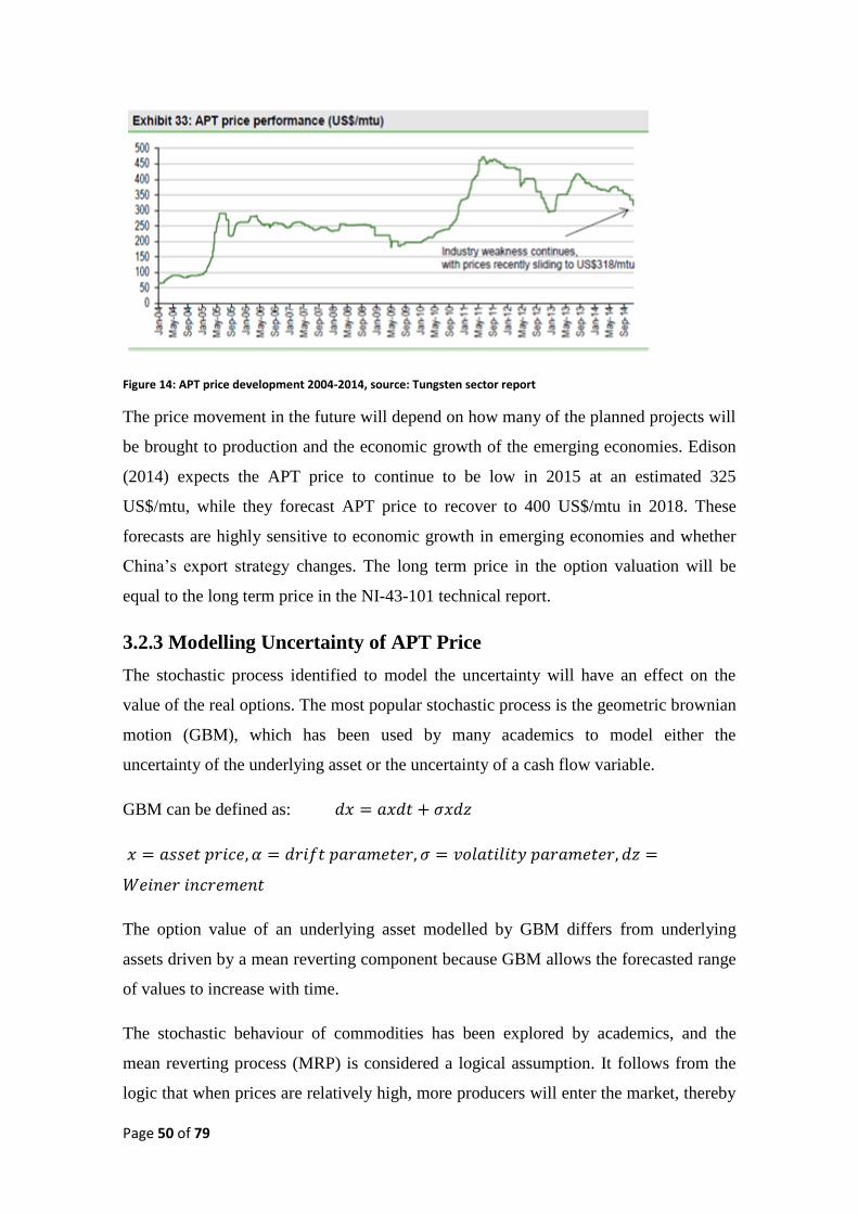
Page 50 of 79
Figure 14: APT price development 2004-2014, source: Tungsten sector report
The price movement in the future will depend on how many of the planned projects will
be brought to production and the economic growth of the emerging economies. Edison
(2014) expects the APT price to continue to be low in 2015 at an estimated 325
US$/mtu, while they forecast APT price to recover to 400 US$/mtu in 2018. These
forecasts are highly sensitive to economic growth in emerging economies and whether
China’s export strategy changes. The long term price in the option valuation will be
equal to the long term price in the NI-43-101 technical report.
3.2.3 Modelling Uncertainty of APT Price
The stochastic process identified to model the uncertainty will have an effect on the
value of the real options. The most popular stochastic process is the geometric brownian
motion (GBM), which has been used by many academics to model either the
uncertainty of the underlying asset or the uncertainty of a cash flow variable.
GBM can be defined as:
The option value of an underlying asset modelled by GBM differs from underlying
assets driven by a mean reverting component because GBM allows the forecasted range
of values to increase with time.
The stochastic behaviour of commodities has been explored by academics, and the
mean reverting process (MRP) is considered a logical assumption. It follows from the
logic that when prices are relatively high, more producers will enter the market, thereby

Page 51 of 79
putting downwards pressure on the price as supply increases. The opposite is expected
to happen when prices are relatively low. The mean reversion process lets the price
fluctuate in the short-term but in the long-run it will converge to the price related to the
marginal cost of production. Contrarily, it can be said that depletion of natural resources
would lead to an upwards trend in commodity prices. However, this could be negated
by technological advances, making it economically viable to extract resources which
were previously considered uneconomical (Ozorio 2012). In this case the theory of the
stochastic processes is inconclusive, therefore I will conduct a test for mean reversion.
MRP can be described by the Ornstein-Uhlenbeck model:
A widely applied tool to test for mean reversion is the Unit Root Test (Augmented
Dickey-Fuller Test). The purpose is to see if the sample (natural logarithm of 503
weekly observations) is stationary (series evolve around a constant mean) or non-
stationary.
The hypothesis: h0: natural log of APT price has a unit root. The t-statistic is -1.996 (P-
value 0.289), which should be compared to the ADF test statistic. This means that the
existence of unit root cannot be rejected at a 10% level. The sample is not stationary
(Ozorio 2012). The model can handle a trend in the test equation, although this was
insignificant and left out. The intercept was significant and included. The data was also
tested for unit root using quarterly observations, yielding the same result.8
The sample was tested for autocorrelation using the Durbin-Watson statistic, which was
2.01, with a test statistic of 2 indicating no autocorrelation. This means the sample does
not exhibit autocorrelation..9
When using the unit root test, a very long series of data could be required to reject the
hypothesis that the data follows a GBM process. Dixit & Pindyck (1994) first used 30-
8 See appendix G
9 See Appendix G
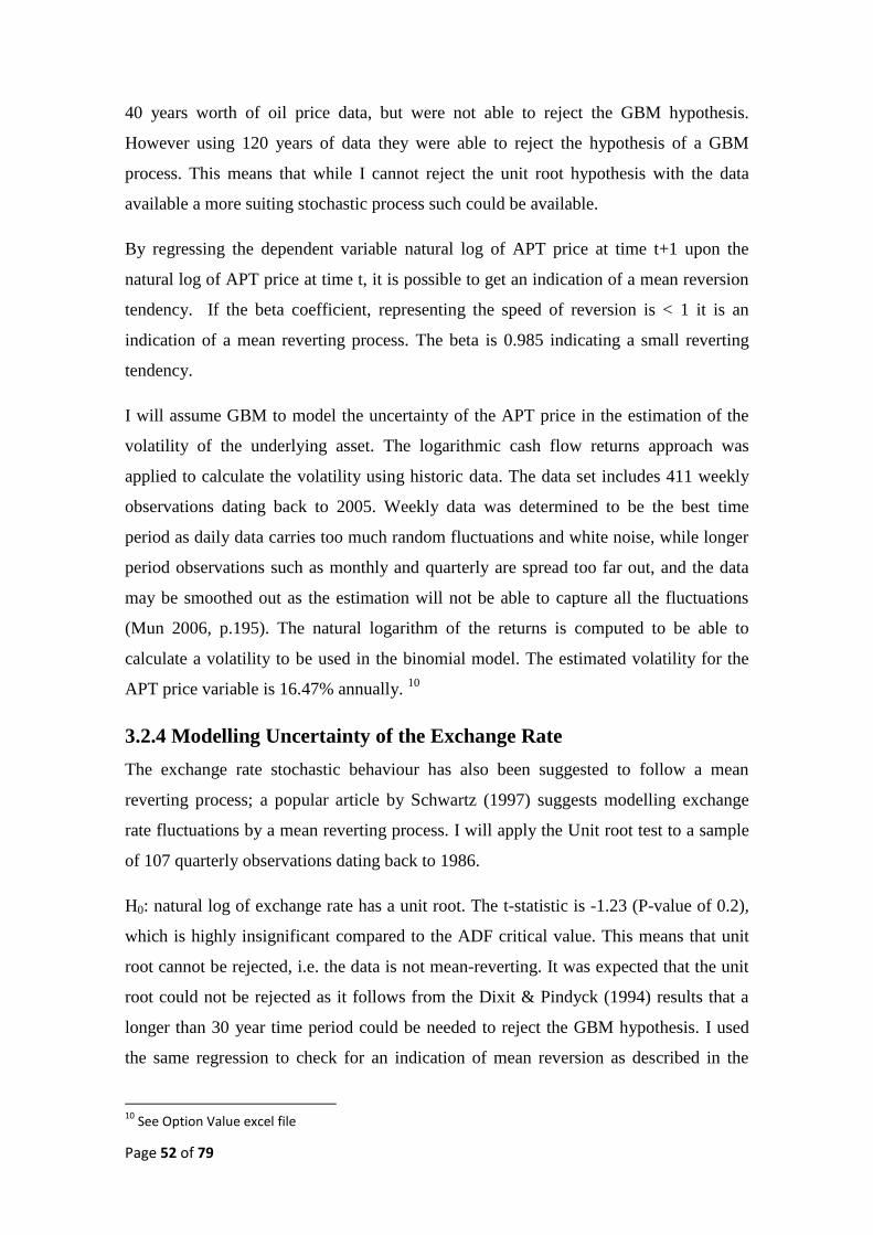
Page 52 of 79
40 years worth of oil price data, but were not able to reject the GBM hypothesis.
However using 120 years of data they were able to reject the hypothesis of a GBM
process. This means that while I cannot reject the unit root hypothesis with the data
available a more suiting stochastic process such could be available.
By regressing the dependent variable natural log of APT price at time t+1 upon the
natural log of APT price at time t, it is possible to get an indication of a mean reversion
tendency. If the beta coefficient, representing the speed of reversion is < 1 it is an
indication of a mean reverting process. The beta is 0.985 indicating a small reverting
tendency.
I will assume GBM to model the uncertainty of the APT price in the estimation of the
volatility of the underlying asset. The logarithmic cash flow returns approach was
applied to calculate the volatility using historic data. The data set includes 411 weekly
observations dating back to 2005. Weekly data was determined to be the best time
period as daily data carries too much random fluctuations and white noise, while longer
period observations such as monthly and quarterly are spread too far out, and the data
may be smoothed out as the estimation will not be able to capture all the fluctuations
(Mun 2006, p.195). The natural logarithm of the returns is computed to be able to
calculate a volatility to be used in the binomial model. The estimated volatility for the
APT price variable is 16.47% annually. 10
3.2.4 Modelling Uncertainty of the Exchange Rate
The exchange rate stochastic behaviour has also been suggested to follow a mean
reverting process; a popular article by Schwartz (1997) suggests modelling exchange
rate fluctuations by a mean reverting process. I will apply the Unit root test to a sample
of 107 quarterly observations dating back to 1986.
H0: natural log of exchange rate has a unit root. The t-statistic is -1.23 (P-value of 0.2),
which is highly insignificant compared to the ADF critical value. This means that unit
root cannot be rejected, i.e. the data is not mean-reverting. It was expected that the unit
root could not be rejected as it follows from the Dixit & Pindyck (1994) results that a
longer than 30 year time period could be needed to reject the GBM hypothesis. I used
the same regression to check for an indication of mean reversion as described in the
10
See Option Value excel file

Page 53 of 79
APT price uncertainty section. The beta coefficient is 0.97 indicating a small mean
reversion. The exchange rate will be modelled as a GBM process in the Monte Carlo
simulation to estimate the volatility of the underlying asset.
As in the APT price analysis, the sample was tested for autocorrelation, yielding a DW
value of close to 211
, which allows me to conclude the sample does not suffer from
autocorrelation.
The exchange rate volatility was estimated using the logarithmic cash flow returns
approach using historic weekly data dating back to 2005. The calculated volatility
estimate is 10.65%
3.2.5 Correlation of Uncertainty Variables
To estimate the correlation of the two uncertainty variables, Monte Carlo simulation
was employed to calculate the spearman correlation coefficient. The estimated
correlation coefficient of the APT price and exchange rate is -52%12
. This means that
there is a moderate negative correlation between the two variables, so an increase in
APT price will be associated with smaller decrease in exchange rate.
3.2.6 Volatility Estimate of the Underlying Asset
A Monte Carlo simulation based on the estimates calculated in the uncertainty section
was conducted. The APT price and exchange rate was modelled as lognormal
distributions, with a mean defined by the NPV calculation long term price, the standard
deviation is the estimated volatility factor for each uncertainty variable. The uncertainty
variables were modelled as correlated, using the spearman correlation coefficient. The
forecast variable (i.e. dependent variable) was set as the variable z, calculated as
, with a constant to allow the time 1 variables to vary in the
simulation. This will allow me to calculate the standard deviation of the percent changes
in the value of the underlying project from time 0 to time 1. This is the volatility of the
underlying, enabling me to build the event tree (Copeland & Antikarov 2003).
11
Appendix G 12
Appendix I

Page 54 of 79
The standard deviation of the Sisson Project is estimated at 0.26, representing a
volatility of 26%. The NPV was estimated to be above 0 for 91.87% of the simulations,
with a simulated minimum of C$ -458.876 M and a maximum of C$ 1.387.756 M. 13
3.3 Event Tree
An event tree (evolution of the underlying) has to be created to model the uncertainty of
the Sisson Project and as an aid to solve the binomial lattice of the option value. The
event tree represents the value the Sisson Project might take as it evolves through time.
Assuming the value of the project follows a GBM, as is widely accepted as a standard
assumption for option pricing (Mun 2006, p. 137), the up and down factors are
determined as: u = = = 1.297 and d = = 1/u = 0.77114
, Where
is the time-steps. S0 = C$ 1,064.052 M
3.4 Create Decision Tree
The management is assumed to be able to abandon the project throughout the life time
of the project, as well as having the ability to contract the output level throughout the
life of the mine. The possibility to defer the project was considered and the option value
estimated15
, however, the option to defer would not be exercised before year 16,
therefore it was excluded. This was done knowing that “Neglecting a particular option
while including others may not necessarily cause significant valuation error” Trigeorgis
(1993). In addition, it seems unrealistic to assume that the management would defer a
positive NPV project for such a long time period.
Figure 15: Event tree representation and binomial option lattice representation, source: Cox, Ross, Rubinstein 1979
13
See appendix J 14
See Option Value Excel Sheet 15
See Option Value Excel Sheet

Page 55 of 79
Using the event tree, a binomial lattice of the option value can be calculated applying
the risk-neutral probability to calculate the binomial lattice value of the option.
The following input values have to be determined:
Value of underlying asset(S) = Present value of operating net income = C$ 1,064.052 M
Exercise price (X) = present Value of capital expenditure = C$ 722764 M
Volatility of the natural logarithm of the underlying free cash flow returns in percent (σ)
= Standard deviation of the Sisson Project = 26%
Time to expiration in years (T) = Life time of the Sisson Project = 29 years
Risk-free rate (rf) = 1.76%
The risk-neutral probability P =
is applied in the backwards induction
analysis = to calculate the binomial option value
lattice. The value at each step was calculated by maximizing the value of keeping the
option open or exercising the option.
3.5 Estimate Value of Real Options
3.5.1 Abandonment Option with Changing Strikes
The option to abandon has been studied by several academics to determine whether it is
valuable. Colwell, Henker and Ho (2003) find that closure options are economically
significant in their empirical analysis. This is supported by Berger, Ofek and Swary
(1996) who finds strong support for the real options abandonment theory predictions of
companies being able to abandon its operations for a salvage value when operating
income is worse than expected. This is also studied by Moel and Tufano (2002), they
show that the option to close down mining operation was exercised for stated-economic
reasons by 20% of operating mines in their sample.
The value of the abandonment option is the maximum value of abandoning or
continuing operations. Continuing operations is the value determined by the lattice of
the underlying. The value of the abandonment is determined by the cost of closure and
the salvage value. The costs of closure involve decommissioning, reclamation and
closure of the mine, as required by provincial and federal legislation and regulation. The

Page 56 of 79
closure costs will grow each year of the life of the mine, ending in a value of C$ 50
million if the mine closes at year 27 of production as reported in the NI-43-101
Technical report. The closure costs will be estimated by a linear function of the C$ 50
million over the 29 year life of the mine. This equates to 1.724 million in closure costs
in the first year of production, rising each year by the same amount.
The salvage value will be estimated as 50% of present value of accumulated capital
expenditure at the time of abandonment, less 10% annual depreciation. The salvage
value also accounts for the present value additional capital investments not yet
undertaken at the time of abandonment. This method has been employed by Trigeorgis
(1996) for valuing a natural resource investment opportunity considered by a
multinational company.
The value of the option to abandon the project during the life time of the mine is valued
at C$ 2.4 M16
3.5.2 Option to Contract with Changing Strikes
The option to contract the output of the mine can be valued as a put option on a
proportion of base scale output with an exercise price equal to the cost savings from
reducing the mineral output of the mine. The mine is assumed to be able to contract its
output, leading to savings in operating costs due to scale backs and potential
remuneration savings. I conducted a thorough review of existing literature on output
contractions in mining to estimate the cost savings involved in an output contraction,
however, academic articles are often hypothetical or theoretical, as company financials
are proprietary. Trigeorgis (1993) suggests that management can operate at a contracted
capacity, which will enable the company to save planned investment outlays, i.e. the
exercise price will be the potential cost savings from the contraction. I have assumed
that Northcliff is able to contract their output by 50%, resulting in 25% savings of
present value yearly operating costs plus the full present value of further planned capital
expenditures in the years after contraction.
The value of the option to contract output by 50% is valued at C$ 49.43 M17
16
Option Value excel Sheet 17
Option Value Excel Sheet

Page 57 of 79
3.5.3 Real Options Interactions and Non-additivity
The two options are mutually exclusive as they cannot both be exercised at the same
time (Mun 2006). This means that the combined option value is not the sum of the two
separate options. The degree of interaction can be either small or large, resulting in a
combined option value, which can be close to the sum of the two separate options or
close to the value of one of the individual options. Valuing the options as the sum of the
two separate options can lead to overestimating the value of the options. The degree of
interaction depends on the type of options being valued, depending on whether it is a
put and a call option or of they are of the same type. Further, the degree of interaction is
decided by the time overlap of the options, the separate degree of being in the money
and the timing of the options. When the options types are opposites (i.e. a put and a call)
they will be exercised opposite to each other as uncertainty unfolds. This means that the
degree of interaction is small and the two options will be largely additive. Alternatively,
if the options are of the same type, the degree of interaction would be large and the
value of options is less additive (Trigeorgis 1993). This means that the value of the
option to abandon and the option to contract, valued as a combined option, will be less
than the sum of the two as they are both put options.
The option to abandon and the option to contract the project valued in combination is
valued at 49.5 C$ M18
, showing a small degree of interaction between the two put
options. Using the real options framework the value of the project has increased by
14.5%.
eNPV value = NPV + options premium = 341.29 + 49.5 = C$ 391 M.
3.5.4 Options Sensitivity Analysis
To analyse the sensitivity of the option premium to deviations from the assumptions
underlying the combined option premium, 4 variables affecting the option value was
adjusted by -50% to +50% from the base case scenario. This will allow me to determine
which variables the option premium is the most sensitive towards if the variables
deviate from the assumptions. At first the risk-free rate was subjected to the
adjustments, the option value reached a maximum of C$ 64.55 M, or a 30% increase in
total option value when the risk-free rate was adjusted upwards by 50%, equalling a
risk-free rate of 2.64%.
18
Option Value Excel Sheet
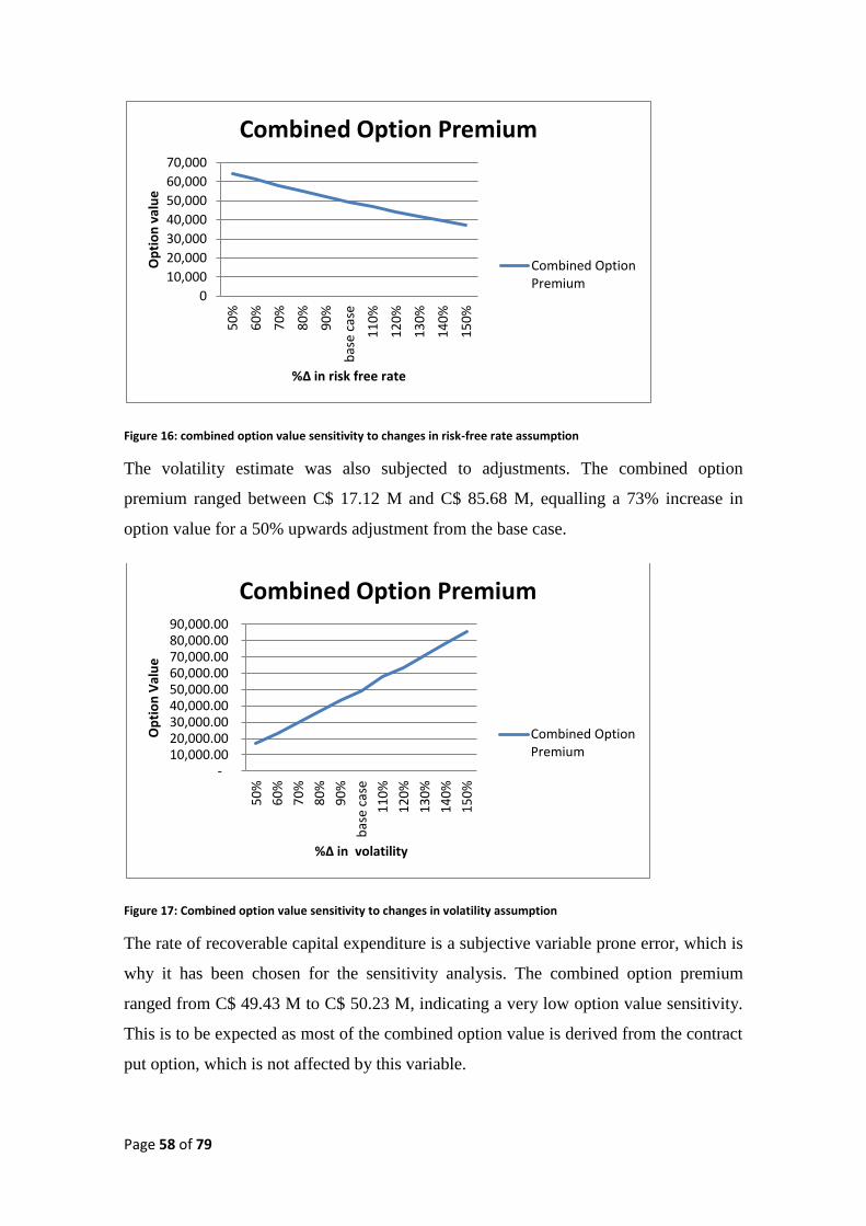
Page 58 of 79
Figure 16: combined option value sensitivity to changes in risk-free rate assumption
The volatility estimate was also subjected to adjustments. The combined option
premium ranged between C$ 17.12 M and C$ 85.68 M, equalling a 73% increase in
option value for a 50% upwards adjustment from the base case.
Figure 17: Combined option value sensitivity to changes in volatility assumption
The rate of recoverable capital expenditure is a subjective variable prone error, which is
why it has been chosen for the sensitivity analysis. The combined option premium
ranged from C$ 49.43 M to C$ 50.23 M, indicating a very low option value sensitivity.
This is to be expected as most of the combined option value is derived from the contract
put option, which is not affected by this variable.
0
10,000
20,000
30,000
40,000
50,000
60,000
70,000
50
%
60
%
70
%
80
%
90
%
bas
e ca
se
11
0%
12
0%
13
0%
14
0%
15
0%
Op
tio
n v
alu
e
%Δ in risk free rate
Combined Option Premium
Combined Option Premium
- 10,000.00 20,000.00 30,000.00 40,000.00 50,000.00 60,000.00 70,000.00 80,000.00 90,000.00
50
%
60
%
70
%
80
%
90
%
bas
e ca
se
11
0%
12
0%
13
0%
14
0%
15
0%
Op
tio
n V
alu
e
%Δ in volatility
Combined Option Premium
Combined Option Premium

Page 59 of 79
Figure 18: Combined option value sensitivity to changes in rate of recoverable capital expenditure assumption
The fraction of further capital expenditure savings from contracting the output was
subjected to an adjustment of -50%, then going back to the base case scenario, in 10%
increments, as it is impossible to save more than the full value of the planned capital
expenditure. The value was estiamted at C$ 2.4 M in the 50% to 80% range of capital
expenditure savings, going up to 23.1 C$ M at 90%, and back to the base case option
value of C$ 49.5 M at a 100%.
Figure 19: Combined option value sensitivity to changes in the fraction of savings of further present value capital expenditure costs
49,000.00
49,500.00
50,000.00
50,500.00
50
%
60
%
70
%
80
%
90
%
bas
e ca
se
11
0%
12
0%
13
0%
14
0%
15
0%
Op
tio
n V
alu
e
%Δ in rate of recoverable capital expenditure
Rate of recoverable capital expenditure
Combined Option Premium
-
20,000.00
40,000.00
60,000.00
50% 60% 70% 80% 90% base case
Op
tio
n V
alu
e
%Δ in the fraction of savings of further present value capital expenditure costs
Fraction of further PV capital expenditure savings
Combined Option Premium
Page 60 of 79
From the sensitivity analysis it can be concluded that the combined option premium is
highly sensitive to the volatility estimate and the fraction of which the project can save
further capital expenditures following a contracting of output.
4. Conclusions
4.1 Main insights
This case study showed how to improve upon the traditional valuation framework to
achieve a capital budgeting process consistent with an uncertain environment. The
thesis highlighted how the traditional NPV model underestimates the value of an
investment project with options. The valuation framework in the thesis utilised the
standard NPV model to support the real options valuation by using the NPV value as the
underlying asset value without flexibility in the real options model. The options
available to the management were shown to be valuable, which corroborates the real
options theory of valuable options in an uncertain environment. Further, the case study
highlighted the points made by Trigeorgis (1993), showing that multiple options have to
be valued in a setting which recognizes the degree of interaction of the real options to
avoid overestimating the value of the combined options.
The sensitivity analysis showed that the project value was highly sensitive towards two
variables and the assumptions made in the thesis. The volatility was estimated after
making a number of choices regarding the length of the estimating period, the length of
the periods used as well as the method for calculating the volatility itself. These choices
and assumptions have a direct effect on the volatility estimate. The sensitivity analysis
highlighted the importance of recognizing that the volatility measure is an estimate,
which could deviate from the true volatility. Finally, the savings from a contraction in
output was shown to be a major driver of the combined option value.
4.2 Conclusion
The thesis initially explored the properties of a capital budgeting process able to handle
both flexibility and uncertainty. The eNPV framework was identified as is it was shown
to be the only framework able to handle both the options available to an active
management as well as the consequences of assuming an uncertain environment. Firstly,
the NPV model was applied to calculate the value of the project without flexibility, as
Page 61 of 79
well as identifying the most sensitive variables in the analysis. Secondly, the variables
chosen as the most influential variables were analysed and modelled to be incorporated
in a Monte Carlo simulation to model to uncertainty of the project. Finally, a decision
tree was built to graphically represent the decision nodes of the two options. The value
of the combined options were estimated at C$ 49.5 M, which represents a 14.5%
increase in project value. The thesis highlighted the limitations of traditional capital
budgeting processes as well as showing a practical application method for real options
valuation to improve the capital budgeting process in companies. This is achieved by
capturing the value of uncertainty and recognizing that the world is uncertain in nature,
requiring a more nuanced capital budgeting process. The consequences of different
scenarios can be recognized and a strategy can be implemented to take advantage of the
knowledge provided by the real options analysis.
4.3 Limitations and Further Research
The thesis was written from an external perspective, therefore only publicly available
information was considered for the valuation. Northcliff is trying to agree upon offtake
agreements for their output, which would lower the option value, depending on how
much output is agreed upon in a contract and the duration of the contract. The NI-43-
101 technical report mentions that no offtake agreements had been signed at the time of
the report drafting. It should be mentioned that the report considers both price volatility
and exchange rate fluctuations as risk factors. In the calculations, assumptions regarding
the financial data had to be made (i.e. effective tax rate and exchange rates over the first
4 years). To create a closer representation of reality, proprietary information would be
needed. However, this is the case in all valuation frameworks, not just the real options
framework. The assumptions made regarding the options available to the management
could have a major influence on the final option valuation. This is true for the
abandonment option as well as the contract option. It has been shown by Moel &
Tufano (2002) that management exhibits hysteretic behaviour in the decision to
abandon a mine, which could lower the actual option value as the management deviates
from the optimal decision strategy (Copeland & Tufano 2004). The option to contract
the output also depends on management actually being able to contract the output, and
realize the savings assumed in the case study. Therefore, there is a need for further
research in real options value where more information regarding the actual options
considered by the management is disclosed. In addition, more information about the

Page 62 of 79
exercise price of option would yield a more accurate value of the options. Lastly,
research into how a cohesive and standard real options framework should be applied is
needed, especially in regards to the analytical approaches described in the thesis.
In closing I want to highlight that unlike financial option valuation, a real options
analysis will not be able to estimate a precise value of the options. Instead, Miller &
Park (2002) suggest that real options analysis should be utilised to identify the options,
the timing of the options and an estimate of the value of the options. The real options
analysis will then provide the manager with a guide to choose the most appropriate
strategy given the identified options.

Page 63 of 79
5. References
Alexander, G & Chervany, N, 1980, On the Estimation and Stability of Beta, Journal of
Financial and Quantitative Analysis, Vol. 15, pp. 123-137.
Amram, M & Kulatilaka, N, 1999, Real Options: Managing Strategic Investments in an
Uncertain World, Harvard Business School Press, Harvard, Cambridge, Massachusetts.
Berk, J & DeMarzo,P, 2011, Corporate Finance, 2nd edition, Pearson Education
Limited, Essex, England.
Berger, P, Ofek, E & Swary, I, 1996, Investor Valuation of the Abandonment Option,
Journal of Financial Economics, No. 42, pp. 257-287.
Black, F & Scholes, M, 1973, The Pricing of Options and Corporate Liabilities, Journal
of Political Economy, Vol. 81, No. 3. p.637-654.
Blume, ME, 1975, Betas and Their Regression Tendencies, The Journal of Finance,
Vol. 30, No.3, pp. 785-795.
Borison, A, 2005, A Response to “Real Options: Meeting the Georgetown Challenge,
Journal of Applied Corporate Finance, Vol. 17, No. 2.
Borison, A, 2005, Real Options Analysis: Where are the Emporor’s Clothes?, Journal of
Applied Corporate Finance, Vol. 17, No. 2.
Brennan, M & Schwartz, E, 1985, Evaluating Natural Resource Investments, Journal of
Business, Vol. 58, No. 2, pp. 135-157.
Brealey, R & Myers, SC, 2000, Principles of Corporate Finance, 6th
edition, Irwin-
McGraw-Hill, Boston.
Brown, S, Goetzmann, W & Ross, S, 1995, Survivorship Bias, Journal of Finance, July,
pp.853-873.
Bruner, R, et al., 1998, Best Practices in Estimating the Cost of Capital: Survey and
Synthesis, Financial Practice and Education, vol. 8, pp. 13-28.

Page 64 of 79
Busby, J & Pitts, C, 1997, Real Options in Practice: An Explanatory Survey of How
Decision Makers in Industry Think About Flexibility, Management Accounting
Research, Vol. 8, pp. 169-186.
CBOE Market Statistics 2013. http://www.cboe.com/data/marketstats-2013.pdf
Copeland, E & Antikarov, V, Real Options: Meeting the Georgetown Challenge,
Journal of Applied Corporate finance, Vol 17, No 2.
Cortazar, G & Casassus, J, 1998, Optimal Timing of a Mine Expansion: Implementing a
Real Options Models, The Quarterly Review of Economics and Finance, Vol. 38,
Special Issue, pp. 755-769.
Cortazar, G, Schwartz, E & Casassus, J, 2001, Optimal Exploration Investments under
Price and Geological-Technical Uncertainty: A Real Options Model, R&D
Management, Vol. 31. No. 2.
Cowell, D, Henker, T & Ho, J, 2002, Real Options Valuation of Australian Gold Mines
and Mining Companies, SSRN.
Cox, J, Ross, S & Rubinstein, M, 1979, Option Pricing: A Simplified Approach, Journal
of Financial Economics, Vol. 7, p. 229-264.
Damodaran, A, 2006, Damodaran on Valuation: Security Analysis for Investment and
Corporate Finance, Johm Wiley & Sons, Onc., Hoboken, New Jersey.
Damodaran, A, 2008, What is the risk-free rate? A Search for the Basic building block,
Stern School of Business, New York University.
Damodaran, A, 2012, Investment Valuation: Tools and techniques for determining the
value of any asset, 3nd edition, Wiley, Hoboken, NJ.
Damodaran, A, 2014, Equity Risk Premiums (ERP): Determinants, Estimation and
Implications – The 2014 Edition, March, Stern School of Business.
Damodaran, A, 2015a, Variables Used in Data Set, Reviewed 02/12/2015,
http://people.stern.nyu.edu/adamodar/New_Home_Page/datafile/variable.htm
Damodaran, A, 2015b, Levered and Unlevered Betas by industry, Reviewed
02/13/2015, http://www.stern.nyu.edu/~adamodar/pc/archives/betas12.xls
Page 65 of 79
Davis, G, 1995, An investigation of the under pricing inherent in DCF valuation
techniques, SME annual meeting, Denver USA.
Dixit, AK & Pindyck, RS, 1994, Investment under Uncertainty, Princeton University
Press, UK, Chicester, West Sussey
Dixit, AK & Pindyck, RS, 1995, The Options Approach to Capital Investment, Harvard
Business review, May-June, pp. 105-118
EU Commision Memo, 08/03/2014, WTO Appellate Body confirms: China’s export
restrictions on rare earths and other raw materials illegal, EU Commision, Brussels,
Reviewed 01/30/2015, http://europa.eu/rapid/press-release_MEMO-14-504_en.htm
Fama, EF & French, KR, 1988, Permanent and Temporary Components of Stock Prices,
Journal of Political Economy, Vol. 96, pp. 246-273.
Fernandez, P, Aguirreamalloa, J & Corres, L, 2011, Equity premium used in 2011 for
the USA by Analysts, Companies and Professors: A Survey, Working Paper,
http://papers.ssrn.com/sol3/papers.cfm?abstract_id=1805852&rec=1&srcabs=1822182.
Graham, JR & Campbell, H 2002, How do CFOs make capital budgeting and capital
structure decisions?, Journal of applied corporate finance, vol. 15, no. 1
https://faculty.fuqua.duke.edu/~jgraham/website/SurveyJACF.pdf
Graham, JR & Harvey, CR, 2013, The Equity Risk Premium in 2013, Working Paper,
http://papers.ssrn.com/sol3/papers.cfm?abstract_id=2206538
Haque, A, Toptal E & Lilford E, 2014, A numerical study for a mining project using
real options valuation under commodity price uncertainty, Resources Policy, Vol. 39,
pp. 115-123.
http://www.sciencedirect.com.ez.statsbiblioteket.dk:2048/science/article/pii/S03014207
13001220%20-%20bib29#bib7
Hayes, RH and Garwin, DA, 1982, Managing as If Tomorrow Mattered, Harvard
business review, Vol. 60, No. 3
Hayes, RH & Abernathy, W, 1980, Managing Our Way to Economic Decline, Harvard
Business Review, July-August.

Page 66 of 79
Hertz, D, 1979, Risk Analysis in Capital Investment, Harvard Business Review,
September.
Howell, S & Jagle, A, 1997, Laboratory Evidence on How Managers Intuitively Value
Real Growth Options, Journal of Business Finance & Accounting, Vol. 24, No.7/8, pp.
915-935.
ITIA , 2011, Pricing, International Tungsten Industry Association, London, Reviewed
01/30/2015, http://www.itia.info/tungsten-prices.html
J.P Morgan, 2014, Bridging the gap between interest rates and investments
https://www.jpmorgan.com/cm/BlobServer/JPMorgan_CorporateFinanceAdvisory_Inte
restRatesAnd.pdf?blobkey=id&blobwhere=1320649301116&blobheader=application/p
df&blobheadername1=Cache-
Control&blobheadervalue1=private&blobcol=urldata&blobtable=MungoBlobs
Kester, CW, 1984, Today’s Options for Tomorrow’s Growth, Harvard Business Review
62, 2, March-April, pp. 14-21
Koller,T, Goedhart, M & Wessels, D, 2010, Valuation: Measuring and Managing the
Value of Companies, 5th
edition, John Wiley & Sons, Hoboken, New Jersey.
Schall, LD, Sundem,GL & Geijsbeek Jr, WR, 1978. Survey and Analysis of Capital
Budgeting Methods, Journal of Finance.
Lemelin, B, Sabour, SAA & Poulin, R, 2006, Valuing mine 2 at raglan using real
options, International Journal of Mining, Reclamation and Environment, 20:01, pp. 46-
56.
Magee, J, 1964, How to Use Decision Trees in Capital Investment, Harvard Business
Review, September-October.
Mayer, Z & Kazakidis, V, 2007,Decision Making in Flexible Mine Production System
Design Using Real Options, Journal of Construction Engineering and Management,
Febuary 1.
Merton, RC, 1998, Applications of Option-Pricing Theory: Twenty-Five Years Later,
The American Economic Review, Vol. 88, No. 3, p. 323-349.
Page 67 of 79
Merton, RC, 1973, “Theory of Rational Options Pricing”, Bell Journal of Economics
and Management Science”, Vol 4, No. 1, p. 141-183.
Miller, LT & Park, CS, 2002, Decision making under under uncertainty – Real options
to the rescue?, The Engineering Economist, Vol. 47, No. 2.
http://www.tandfonline.com/doi/pdf/10.1080/00137910208965029
Moel, A & Tufano, P, 2002, When are Real Options Exercised? An Empirical Study of
Mine Closings, The Review of Financial Studies, Vol. 15, No. 1, pp. 35-64.
Mun, J, 2006, Real options analysis: Tools and Techniques for Valuing Strategic
Investments and Decisions, 2nd edition, John Wiley & Sons, Inc., Hoboken, New
Jersey.
Myers, SC, 1977, Determinants of Corporate Borrowing, Journal of Financial
Economics.
Myers, SC, 1987, Finance Theory and Financial Strategy, Midland Corporate Finance
Journal 5, No. 1, pp. 6-13
Ozorio, LDM, Bastian-Pinto, CDL & Brandão, LET, 2012, The Choice of Stochastic
Process in Real Option Valuation.
Poterba, J & Summers, LH, 1991, Time Horizons of American Firms: New Evidence
from a survey of CEOs, (MIT Working Paper).
Ryan, P & Ryan, G, 2002, Capital Budgeting Practices of the Fortune 1000: How Have
Things Changed?, Journal of Business & Management, Oct.
Samis, M, Martinez, L , Davis, GA & White, JB, 2010, Using Dynamic DCF and Real
Options for Economic Analysis in NI43-101 Technical Reports, Inside Mines.
Samuel Engineering, Canadian National Instrument 43-101 Technical Report on The
Sisson Project New Brunswick, Canada.
http://www.sedar.com/DisplayCompanyDocuments.do?lang=EN&issuerNo=00030606
Search: Technical report (NI 43-101) - English
Schwartz, ES, 1997, The stochastic behaviour of commodity prices: implications for
valuation and hedging., Journal of Finance 52 (3),pp. 923–973.

Page 68 of 79
Segelod, E, 1998, A Note on the Surbey of Project Evaluation Techniques in Major
Corporations, International Journal of Production economics, Vol. 54, 2nd
issue, pp.
207-213
Sinocast Metals, Mining & Chemicals Beat , 12/30/2014, China Cancels 2015
Tungsten, Molybdenum Export Quotas, Kitco News, Canada, Reviewed 01/30/2015,
http://www.kitco.com/news/2014-12-30/China-Cancels-2015-Tungsten-Molybdenum-
Export-Quotas.html
Stellmaszek, F, 2010, Real Options in Strategic Decisions: An Empirical Case Study
Analysis of How Companies Integrate Real Options into Strategic Decisions, Pro
Business, Berlin.
Trigeorgis, L & Mason, SP 1987, Valuing managerial flexibility, Midland Corporate
Finance Journal 5, pp. 14-21. Harvard reference
Trigeorgis, L, 1993,Real Options and Interactions with Financial Flexibility, Financial
Management 22, 3, pp. 202-224.
Trigeorgis, L, 1996, Real Options: Managing Flexibility and Strategy in Resource
Allocation, The MIT Press, Cambridge, Massachusetts, London, England.
Trigeorgis,, L, 1998, A conceptual options framework for capital budgeting, Advances
in Futures and Options Research 3, pp.. 145-167.
Triantis, A, 2005, Realizing the Potential of Real Options: Does Theory Meet Practice?,
Journal of Applied Corporate Finance, Vol. 17, No. 2.
Triantis, A & Borison A, 2005, Real Options: State of the Practice, Journal of Applied
Corporate Finance, Vol. 14.2.
Tungsten Market Research ltd., Tungsten Market Summary, Tungsten Market Research,
Reviewed 01/30/2015, http://www.tungstenresearch.com/tungsten.html
Tungsten Sector Report, December 2014, Small sector for big returns, Edison
Investment Research
Van Putten, AB & MacMillan, I, 2004, Making Real Options Really Work, Harvard
Business Review, Dec., https://hbr.org/2004/12/making-real-options-really-work/ar/1
Page 69 of 79
Yin, RK, 2014, Case Study Research: Design and Methods, 5th
edition, Sage Publication
Inc.
6. List of Figures
Figure 1: Comparison of financial and real options, source: Felix Stellmaszek .......................... 22
Figure 2: when are options valuable, Source: Koller, et al. 2010 ................................................ 23
Figure 3: Cone of uncertainty, source: Mun 2006, p.136 .......................................................... 26
Figure 4: Real options solution techniques, source: Kodukula & Papudesu 2006 ...................... 31
Figure 5: 5 step real options methodology, source: Copeland & Antikarov (2005) .................... 36
Figure 6: Capital costs estimate, source: NI-43-101 Technical report ........................................ 39
Figure 7: Sustaining capital costs estimate, source: NI-43-101 Technical report ....................... 40
Figure 8: Historical risk premium, source: Damodaran homepage ............................................ 43
Figure 9: Geometric historical risk premium for different estimation periods, source:
Damodaran (edited) .................................................................................................................... 43
Figure 10: List of companies and their respective unlevered beta and the median industry
unlevered beta ............................................................................................................................ 46
Figure 11: NPV sensitivity analysis .............................................................................................. 47
Figure 12: Tungsten consumption by product, source: Tungsten Sector report ........................ 48
Figure 13: World tungsten demand by region, source: tungsten sector report ......................... 49
Figure 14: APT price development 2004-2014, source: Tungsten sector report ........................ 50
Figure 15: Event tree representation and binomial option lattice representation, source: Cox,
Ross, Rubinstein 1979 ................................................................................................................. 54
Figure 16: combined option value sensitivity to changes in risk-free rate assumption ............. 58
Figure 17: Combined option value sensitivity to changes in volatility assumption .................... 58
Figure 18: Combined option value sensitivity to changes in rate of recoverable capital
expenditure assumption ............................................................................................................. 59
Figure 19: Combined option value sensitivity to changes in the fraction of savings of further
present value capital expenditure costs ..................................................................................... 59

Page 70 of 79
7. Appendix
Appendix A – Cash flow Summary, Mineral Resource, Reserve, price and recovery
assumptions

Page 71 of 79
Appendix B – Design Parameters for Reserve Estimate
Appendix C – Production Schedule Summary

Page 72 of 79
Appendix D – Tax summary

Page 73 of 79
Appendix E – Cost of Capital Summary

Page 74 of 79
Appendix F – Northcliff Resources ltd. Beta Estimate
Dependent Variable: NCF_RETURN
Method: Least Squares
Date: 02/12/15 Time: 11:56
Sample: 6/13/2011 12/31/2012
Included observations: 82
Variable Coefficient Std. Error t-Statistic Prob.
C -0.006231 0.013280 -0.469236 0.6402
TSX_RETURN 0.308013 0.611093 0.504037 0.6156
R-squared 0.003166 Mean dependent var -0.006350
Adjusted R-squared -0.009295 S.D. dependent var 0.119682
S.E. of regression 0.120237 Akaike info criterion -1.374616
Sum squared resid 1.156555 Schwarz criterion -1.315915
Log likelihood 58.35925 Hannan-Quinn criter. -1.351048
F-statistic 0.254053 Durbin-Watson stat 2.070933
Prob(F-statistic) 0.615621
Appendix G – Unit Root Test
Unit root test weekly ln apt price 2003 to end 2012
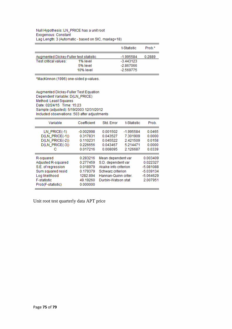
Page 75 of 79
Unit root test quarterly data APT price

Page 76 of 79
Mean reversion regression exchange rate weekly data
Mean reversion regression exchange rate 26 year quarterly data

Page 77 of 79
Appendix H – Variables Correlation
APT price and Exchange rate Spearman correlation
Appendix I – Volatility of Underlying Asset

Page 78 of 79
Appendix J – Dynamic NPV

Page 79 of 79