Value relevant asset measurement and asset

use: Evidence from IAS 41

Adrienna A. Huffman

PhD Candidate

David Eccles School of Business

University of Utah adrienna.huffman@business.utah.edu

November 2013

ABSTRACT: I examine whether asset measurement linked to asset use provides investors with incrementally more value relevant information in a sample of 183 international firms from 35 countries that adopt International Accounting Standard (IAS) 41. IAS 41 prescribes fair value measurement for biological assets, a class of assets previously classified as PP&E and measured at historical cost. I find that book value and earnings information is significantly more value relevant in regressions of stock price, stock returns, and mechanical forecasting models of future operating cash flows and operating income when firms measure their biological assets consistent with their use, relative to when they do not. My findings provide support for early accounting theory that links value relevant asset measurement to the way in which the asset generates value (e.g. Littleton 1935; May 1936), current asset measurement frameworks, and the International Accounting Standards Board’s (2013) recent revisions to the asset measurement section of its conceptual framework. Key words: International accounting; asset measurement; fair value accounting; value relevant information; business valuation. * I would like to thank my dissertation committee, in particular my chair Christine Botosan, Marlene Plumlee, Melissa Lewis, Jim Schallheim, and Haimanti Bhattacharya for all of their support and invaluable feedback. I would also like to thank Steve Stubben for his excellent suggestions and help, and workshop participants at the University of Utah and the Accounting Research Symposium at Brigham Young University. I gratefully acknowledge financial support from the Marriner S. Eccles Graduate Research Fellowship in Political Economy and the David Eccles School of Business. All errors are my own.

1

1. Introduction

Assets generate value via two mechanisms. In-exchange assets (e.g. cash) generate value on a

standalone basis in exchange for cash or other valuable assets, while in-use assets (e.g. property, plant and

equipment (PP&E)) generate value in use in combination with other assets. Early accounting theorists

link value relevant asset measurement to the manner in which an asset generates value (e.g. Littleton

1935). Specifically, this literature claims that fair value applied to in-exchange assets and historical cost

applied to in-use assets has the potential to produce incrementally more value relevant information for

investors. Nevertheless, in some cases, modern accounting standards, do not link asset measurement to

the manner in which the asset generates value. For example, International Accounting Standard (IAS) 41

requires fair value measurement for “biological assets,” which are living plants and animals, regardless of

whether the biological assets derive value in-use or in-exchange.

I use the adoption of IAS 41 as a setting to examine whether asset measurement linked to asset

use provides investors with incrementally more value relevant information. I employ a sample of 183

international firms from 35 countries that adopt IAS 41. In a multi-pronged approach, I assess the value

relevance of book value and earnings information in regressions of stock price, stock returns, future

operating cash flows and future operating income for the firms that measure their biological assets

consistent with their use (consistent measurement sample) and for the firms that measure their biological

assets inconsistent with their use (inconsistent measurement sample). As suggested by some prior

literature, I find that book value and earnings information is more value relevant when asset measurement

is consistent with the manner in which the asset realizes value for the firm, relative to when it is not.

Specifically, I find that book value and earnings information is more value relevant when in-exchange (in-

use) assets are measured at fair value (historical cost) as compared to when in-exchange (in-use) assets

are measured at historical cost (fair value).

Taken together, my findings provide empirical support for the early accounting theory that links

value relevant asset measurement to the way in which the asset generates value (e.g. Littleton 1935; May

1936). Further, my findings support the International Accounting Standards Board’s (IASB) recent

2

revisions to the measurement section of its conceptual framework. Specifically, the IASB (2013a) states

that the relevance and selection of a particular measurement basis depends on how the asset contributes to

the entity’s future cash flows, i.e. is used by the firm, and this occurs either directly (i.e. in-exchange) or

in combination with other assets (i.e. in-use) (¶6.16).

The adoption of IAS 41 offers an advantageous setting to examine the implication of linking asset

measurement to asset use on the value relevance of accounting information, for several reasons. First, the

extent to which assets derive value in-use or in-exchange varies across firms for similar types of

biological assets. For example, some firms grow plantations to produce timber logs (an in-exchange asset)

while other firms grow plantations to produce palm oil (an in-use asset).

Second, when there is a lack of reliable parameters to estimate the fair value of the biological

assets, the standard allows firms to measure their biological assets at historical cost (discussed further in

Section 2.3), although the majority of firms apply fair value measurement as mandated. Thus, upon

adoption of IAS 41, some firms measure their biological assets in a manner consistent with their use (i.e.

historical cost for in-use assets or fair value for in-exchange assets) while others do not (i.e. historical cost

for in-exchange assets or fair value for in-use assets). These combinations allow for a cross-sectional

comparison of biological asset-groups where the asset measurement is consistent with the assets’ use,

versus when it is not for both fair value and historical cost accounting.

Third, IAS 41 mandates the measurement model to be employed. This helps to mitigate the

selection bias in prior research that occurs when firms fair value non-financial assets at discretion (e.g.

Easton et al. 1993; Barth and Clinch 1998; Aboody et al. 1999), or when provided a choice (Cairns et al.

2011; Christensen and Nikolaev 2013). Finally, IAS 41 is a “true” fair value standard: the fair value of

biological assets is reported on the firm’s balance sheet and any change in the fair value of the biological

assets over the reporting period is recognized in periodic income as an unrealized gain or loss. This

mitigates issues related to investors’ perceptions of recognized versus disclosed amounts when firms fair

value non-financial assets in disclosures (e.g. Beaver and Landsman 1983; Ahmed et al. 2006).

3

This paper makes several contributions to the literature. First, to my knowledge, it is the first to

test and provide empirical support for an asset measurement framework that links asset measurement to

asset use. This should be of interest to accounting standard setters since the Financial Accounting

Standards Board (FASB) and the IASB have voiced concern over their lack of a systematic framework to

guide asset measurement standards.1 As a result, asset measurement guidance continues to be a hotly

contested standard setting issue and inconsistencies exist across standards.2 Thus, a framework to guide

standard setters’ asset measurement choices and to support high-quality, consistent standard setting is

greatly needed. I believe my findings provide evidence supporting a systematic framework for asset

measurement that could inform standard setters’ decision-making processes on future asset measurement

standards.

Second, my findings provide evidence that the asset measurement investors find useful in

assessing firm value is sometimes, but not always, fair value, and similarly for historical cost. This is in

contrast to the current academic debate over asset measurement which tends to side exclusively with fair

value or historical cost. By understanding which asset measurement investors find useful in determining

firm value, the accounting community is better positioned to understand cost-benefit tradeoffs and how to

improve the effectiveness of financial statement disclosures; a primary objective of the FASB’s disclosure

framework project (FASB 2012).

Finally, much of the prior literature examining fair value measurement investigates whether fair

value is sufficiently reliable to be value relevant to investors, beyond measurement at historical cost.3

This relative reliability perspective differs from a business valuation perspective, which links value

relevant asset measurement to the manner in which the asset realizes value, not to the relative reliability

1 For example, the opening paragraph of the measurement section from the IASB’s (2013) discussion paper of its conceptual framework states: “The existing Conceptual Framework provides little guidance on measurement and when particular measurement should be used” (¶6.1). 2 The objective of the IASB and FASB’s joint project on an improved conceptual framework for financial reporting is “…for their standards to be clearly based on consistent principles. To be consistent, principles must be rooted in fundamental concepts rather than a collection of conventions” (as quoted in Milburn 2012; from ¶P4, IASB 2008). 3 See, for example, among others: Easton et al. 1993; Barth 1994a,b; Bernard et al. 1995; Barth et al. 1996; Barth and Clinch (1998); Aboody et al. 1999; Song et al. 2010.

4

of the measure. The former perspective, which has its roots in early accounting theory (e.g. Littleton

1935; May 1936), underpins a recent framework for asset measurement proposed in Botosan and

Huffman (2013). In contrast to the relative reliability research, I find that fair value information is more

value relevant for in-exchange biological assets than in-use biological assets. That is, in my study, value

relevance is a function of asset use, not the reliability of the fair value measure.4 I seek to supplement and

contribute to the extant literature by providing evidence regarding the link between value relevant asset

measurement and the manner in which assets realize value.

The remainder of the paper is organized as follows. Section 2 develops the hypothesis, related

literature, and IAS 41 background. Section 3 explains the research design. Section 4 describes the data.

Section 5 presents the results. Section 6 concludes.

2. Hypothesis Development, Related Literature, and Background

This study relates to two primary streams of literature. The first stream of literature develops asset

measurement frameworks from a valuation approach, and suggests that a uniform measurement basis may

not provide investors with all information necessary for business valuation. A second stream provides

evidence on the value relevance of fair value measurement for in-exchange and in-use assets. This paper

empirically tests the link between these two streams of literature by examining whether decision-useful

asset measurement is linked to the manner in which the asset generates value for the firm.

2.1 A Business Valuation Framework for Asset Measurement

The asset measurement framework I adopt suggests that the asset measurement that is decision-

useful to investors is a function of how the asset is expected to realize value for the firm. Value realization

occurs via two mechanisms: in-exchange or in-use (Botosan and Huffman 2013, hereafter BH). In-

exchange assets are expected to realize their contribution to firm value on a standalone basis in exchange

for cash or other economically valuable assets. In-exchange assets derive no additional value from being

4 The fair value of both in-exchange and in-use biological assets is often measured using a discounted cash flow approach, considered a “Level 3” estimation as defined by Statement of Financial Accounting Standard (SFAS) 157 (FASB 2006). Research suggests that investors perceive Level 3 estimates as less reliable than “Level 1” or “Level 2” estimates of fair value, which employ market prices (e.g. Kolev 2009; Song et al. 2010).

5

used in combination with other assets. In contrast, in-use assets are expected to realize their contribution

to firm value employed in combination with other assets. This combination of assets can be referred to as

a “cash generating unit.” The in-use value of the cash generating unit is expected to exceed the sum of the

individual assets’ standalone exchange values (Fortgang and Mayer 1985).

BH employ the following standard model for determining firm value (Vt) to develop their

business valuation framework for asset measurement:5

�� = ��� + ∑ ���� �̃����

���� (1)

Where: ��� = in-exchange assets net of non-operating liabilities, date t. � = one plus the risk-free interest rate. �� = expectation formed based on available information, date t. �� = cash flows from in-use assets, net of investments in those activities, date t.

Equation (1) demonstrates that firm value (Vt) is equal to the value the firm’s net in-exchange

assets generate plus the value the firm’s in-use assets generate, net of investment in those activities.

Because in-exchange assets derive value on a standalone basis, BH conclude from equation (1) that fair

value measurement for in-exchange assets will provide investors with the most decision-useful

information to assess the value in-exchange assets generate for the firm.

Because in-use assets generate value beyond the sum of the individual assets’ standalone

exchange values, the value in-use assets generate in equation (1) is represented by the sum of the

discounted cash flows expected to be generated from the in-use assets used in combination with other

firm assets. The excess value in-use assets generate, beyond the sum of the individual assets’ standalone

exchange values, is sometimes referred to as “goodwill” (Feltham and Ohlson 1995; Hitz 2007). This

notion is captured by equation (2) below:

∑ ���� �̃����

���� = �(���, ��) (2)

Where: ��� = in-use assets net of operating liabilities, date t. �� = goodwill.

All other variables are defined above.

5 This model is presented in most valuation textbooks (e.g. pg 13-16, Easton et al. 2013).

6

In equation (2) goodwill (��) is the incremental value created by using assets in combination.

This incremental value is a joint value. Therefore, it is not possible to meaningfully allocate the goodwill

to individual in-use assets because this incremental value is created by the assets used in combination.

Consequently, BH argue that the in-use value for an asset cannot be meaningfully estimated independent

of the other assets in the cash generating unit.

For example, it is possible to estimate the present value of the future cash flows generated by

machinery, materials, and labor (a cash generating unit), which produces a product sold to produce net

cash inflows for the firm. The resulting value is expected to exceed the sum of the individual market

exchange values of the machinery, materials and labor but that excess value cannot be meaningfully

attributed to any individual asset(s) since it is created by using the assets in combination with one another.

From equations (1) and (2), it becomes apparent that from a business valuation perspective

investors require the following information. First, they require sufficient information to allow them to

assess the market values of in-exchange assets and financial obligations. Second, investors require

sufficient information to allow them to form reliable expectations regarding the future cash flows to be

realized from in-use assets, net of investments in those activities. In particular, (2) demonstrates that the

asset measurement that would faithfully represent the value of an in-use asset is value-in-use, but because

this value is only realized in combination with the firm’s other productive assets, it is not determinable on

a standalone basis. Consequently, BH conclude that fair value measurement will provide investors with

decision-useful information to forecast the value in-exchange assets generate, but fair value measurement

will provide investors with relatively less decision-useful information to forecast the value in-use assets

create. I empirically test the validity of these predictions employing the adoption of IAS 41 and I

operationalize decision-useful information as the comparative value relevance of financial information for

the consistent and inconsistent measurement samples.

The predictions from the BH model are consistent with the IASB’s (2013a) recent revisions to the

measurement section of its conceptual framework. The IASB (2013a) states that the relevance and

7

selection of a particular measurement basis depends on how the asset contributes to the entity’s future

cash flows, i.e. is being used by the firm (¶6.16). Some assets contribute cash flows directly (i.e. derive

value in-exchange) while some assets are used in combination with other assets (i.e. derive value in-use)

(¶6.16a-¶6.16b, IASB 2013). The IASB (2013a) asserts that users of financial statements are likely to find

information about the asset’s current market price useful in assessing in-exchange assets’ contribution to

firm value, but for in-use assets, current market prices may not provide investors with relevant

information (¶6.16a-¶6.16b). Instead, for in-use assets, the IASB (2013a) states, users will often use cost-

based information about transactions and past margins to assess how the assets will contribute to the

entity’s future cash flows (¶6.16b). I test these assertions empirically to investigate whether asset

measurement is linked to the manner in which the asset generates value provides investors with more

value relevant information.

Finally, other asset measurement frameworks that take a business valuation perspective reach

similar conclusions to BH. Specifically, Nissim and Penman (2008) argue that fair value accounting is

sufficient for reporting to shareholders only when the firm does not add value to the input through its

business model (Principle 1). A firm does not add value to the input through its business model when the

asset is bought and sold in the same market, i.e. an in-exchange asset. Otherwise, Nissim and Penman

(2008) maintain that historical cost accounting is designed for business models where the firm transforms

inputs to add value, i.e. in-use assets. Nissim and Penman (2008) argue that under historical cost, the

value in-use assets generate will be better represented by the value they create for the firm upon sale of

the final product, as a revenue, instead of individually measured at fair value on the balance sheet.

In addition, a measurement framework developed by the Institute of Chartered Accountants in

England and Wales (ICAEW, 2010) advocates for market exchange values for assets that are not being

used or created within the firm (¶3.2), i.e. assets that derive value in-exchange. Otherwise, the ICAEW

(2010) framework also advocates for historical cost accounting as the most relevant measurement basis

when the firm’s business model is to transform inputs so as to create new assets or services as outputs.

2.2 Relation to Prior Literature

8

Consistent with the BH framework, prior research has repeatedly established the value relevance

of fair value measurement for a specific class of in-exchange assets: financial securities.6 Moreover, these

findings extend to investors’ use of fair value measurement information for in-exchange assets under all

three levels of the fair value measurement hierarchy defined by Statement of Financial Accounting

Standard (SFAS) 157: market exchange value (Level 1), market exchange value adjusted for specific

asset characteristics (Level 2), and fair value measured using valuation techniques (Level 3) (Kolev 2009;

Song et al. 2010). Accordingly, the value relevance of fair value information is not simply a function of

measurement reliability.

Research regarding equity investors’ use of fair value measurement for in-use assets, however, is

burdened by the lack of measurement variation across in-use asset classes. Accordingly, early research

examining investors’ use of fair value information for in-use assets examines disclosed current cost

estimates for firms’ PP&E required under SFAS 33. This research fails to find that current cost

disclosures are value relevant (e.g. Beaver and Landsman 1983; Beaver and Ryan 1985; Bernard and

Ruland 1987; Hopwood and Schaefer 1989; Lobo and Song 1989). The lack of relevance, however, could

be attributed to investors’ perceptions of disclosed values as less reliable or relevant than recognized

amounts (e.g. Ahmed et al. 2006).

Later research examining investors’ use of fair value measurement for in-use assets employs

settings in which U.K. and Australian firms made discretionary and infrequent revaluations to their

tangible long-lived assets. The research findings are mixed. Easton et al. (1993) find that Australian

firms’ asset revaluations of in-use assets are value relevant, but not associated with the firms’ future

return performance. Barth and Clinch (1998) find that the value relevance of Australian firms’

revaluations of long-lived assets depends on both the firm’s industry and asset class after controlling for

measurement at historical coast (see Table IV). Aboody et al. (1999) find that U.K. firms’ revaluation

6 These studies consistently find that investors perceive fair value estimates for financial securities as more value relevant than historical cost amounts: Barth 1994a, b; Ahmed and Takeda 1995; Bernard et al. 1995; Petroni and Whalen 1995; Barth et al. 1996; Eccher et al. 1996; Nelson 1996.

9

activity is significantly associated with the firms’ future operating performance. As Christensen and

Nikolaev (2013) argue, however, a problem with discretionary asset revaluations is that managers decide

to revalue ex-post and therefore may revalue for a host of reasons that are unrelated to providing investors

with decision-useful information, i.e. when they need to manage reported performance.

Further, few financial accounting standards mandate measurement of in-use assets at fair value;

international accounting standards provide firms with a choice of measurement at cost or fair value for

several classes of in-use assets.7 Accordingly, more recent research on fair value measurement of in-use

assets examines firms’ measurement choice for non-financial assets upon adoption of IFRS. Both Cairns

et al. (2011) and Christensen and Nikolaev (2013) find that few U.K., Australian, and German firms

choose to measure their non-financial assets at fair value upon adoption of IFRS. In particular,

Christensen and Nikolaev (2013) find that firms continue to measure their investment property at fair

value, consistent with the prior U.K. GAAP standard SSAP 19, but almost exclusively choose cost

measurement for intangibles and PP&E asset classes (i.e. in-use assets).

This result contradicts Christensen and Nikolaev’s original hypothesis that upon IFRS adoption,

most firms would move to fair value measurement for non-financial assets. Once more, the lack of an

asset measurement framework that predicts when fair value provides investors with decision-useful

information becomes apparent. Consequently, empirically assessing the relevance, or lack thereof, of fair

value measurement for in-use assets is challenging.

2.3 IAS 41

The recent passage of IAS 41 offers a unique setting to test investors’ use of fair value

measurement for in-exchange and in-use assets because it requires fair value measurement for biological

7 U.K. GAAP mandated fair value measurement of investment property, an in-use asset, pre-IFRS. Upon adoption of IFRS, however, firms were given a choice to measure investment property at cost or fair value under IAS 40. Almost all UK, and German, real estate firms, with large holdings of investment property, continued to measure the assets at fair value (Muller et al. 2011). Again, this provides little variation in asset measurement across in-use assets.

10

assets, an asset class that prior to IFRS was not governed by any unified accounting standard.8 IAS 41

prescribes accounting treatment for biological assets, which are living plants and animals.9 Biological

assets are held by firms involved in agricultural activity. Agricultural activities that produce or employ

biological assets include raising livestock, forestry, cropping, cultivating orchards and plantations,

floriculture and aquaculture (¶6, IASB 2009). IAS 41 became effective for annual reporting periods

beginning on or after January 1, 2003, or alternatively, upon adoption of IFRS.

In contrast, U.S. GAAP does not use the term “biological assets” in its accounting for agricultural

producers (KPMG 2008). U.S. GAAP prescribes accounting treatment for “growing crops” and “animals

being developed for sale,” which would be characterized as “biological assets” under IAS 41 (KPMG

2008). Unlike IAS 41, “biological assets” under U.S. GAAP are stated at the lower of cost and market and

classified as inventory (KPMG 2008).

In certain situations, IAS 41 allows firms to measure biological assets at historical cost if the firm

is able to demonstrate that the fair value of its biological assets cannot be reliably estimated, i.e. there is a

lack of reliable parameters such as known prices, growth rates or physical volumes of the asset (¶30,

IASB 2009). Although the majority of my sample applies the standard as mandated, I utilize this

measurement variation in my research design. Specifically, 32% of the firm-year observations in my

sample contain biological assets measured at cost, while 68% of the firm-year observations contain

biological assets measured at fair value (see Table 1, Panel A). Therefore, IAS 41 provides variation in

asset measurement while helping to mitigate the selection bias that occurs when firms fair value non-

financial assets in disclosures, at discretion, or when provided a choice.

Further, variation exists in the extent to which firms derive value from biological assets.

Specifically, IAS 41 encourages firms to distinguish between “consumable” and “bearer” biological

8 Pre-IFRS, Australian firms had to account for ‘self-generating and re-generating assets’ under AASB 1037, which is similar to (predates) IAS 41. No other countries, however, prescribed accounting treatment for biological assets pre-IFRS adoption. 9 Specifically, IAS 41 prescribes accounting treatment for agricultural activity, or “management by the entity of the biological transformation of living animals and plants (biological assets) for sale, into agricultural produce, or into additional biological assets” (¶IN1, IASB 2009).

11

assets in order to provide information that may help investors in assessing the timing of future cash flows

(¶43, IASB 2009). This distinction maps closely into the way in which the biological assets are expected

to realize value for the firm. Consumable biological assets are agricultural products, like crops or timber,

or sold as biological assets, like commodities (¶44, IASB 2009). Consumable biological assets realize

value on a standalone basis and are therefore closer to in-exchange assets. Bearer biological assets, on the

other hand, are self-regenerating assets, like orchards or oil palm plantations (¶44, IASB 2009). Bearer

biological assets realize value in combination with other assets and are therefore in-use assets.10

Nevertheless, IAS 41 requires fair value measurement for both in-exchange and in-use biological

assets. Under IAS 41, a firm producing palm oil from oil palm trees measures its oil palm plantations, an

in-use asset, at fair value on the balance sheet, excluding any fair value attributable to the land upon

which the oil palms are physically attached or intangible assets related to the oil palm production (¶2,

IASB 2009). Thus, firms are required to measure and report only the oil palm trees component of the cash

generating unit at fair value. Likewise, a firm that harvests logs from timber plantations, an in-exchange

asset, also measures the timber plantations at fair value every reporting period on the balance sheet, less

any costs to sell. Changes in the fair value of the oil palm plantations or timber (i.e. unrealized holding

gains and losses) are recognized in periodic income (IASB 2009).

Prior to IAS 41, most (albeit not all) firms accounted for biological assets at historical cost.11

Such assets were classified as property, plant and equipment (PP&E) on the balance sheet, and were

subject to impairment analysis. Upon adoption of the standard, firms recognize the value of their

10 Recently, the Asian-Oceanian Standard Setters Group (AOSSG) proposed different accounting treatments for bearer and consumable biological assets because of the differences in the way the asset-types are used by the firm (AOSSG 2011). Specifically, the AOSSG (2011) argues that bearer biological assets are held for income generation (derive value in-use) and therefore should be treated as PP&E, while consumable biological assets are held for sale (derive value in-exchange), and as such should continue to be measured at fair value. In light of the AOSSG paper, the IASB issued an exposure draft proposing to amend IAS 41 with respect to bearer biological assets and account for them as part of property, plant and equipment in accordance with requirements in IAS 16 (IASB 2013b). IAS 16 allows for measurement at cost. 11 As I describe in footnote 8, Australian firms accounted for ‘self-generating and re-generating’ assets at fair value on the balance sheet beginning in fiscal year 2000 under a similar standard that pre-dated IAS 41 (AAB 1037). There are 44 firm-year observations in my sample that account for their biological assets under this standard.

12

biological assets on the balance sheet, separate from PP&E. There is no requirement to disclose

measurement at cost in the footnotes, although a handful of firms do so voluntarily.

2.4 Hypothesis

In testing the BH framework, I expect that asset measurement linked to asset use will provide

investors with relatively more decision-useful information to assess firm value than asset measurement

that is not linked to asset use. In their joint conceptual framework for financial reporting, the FASB and

the IASB characterize financial information as decision-useful if it is relevant and faithfully represents

what it purports to represent (¶QC4, IASB 2010). Relevant information, as characterized by the

conceptual framework, is financial information that is capable of making a difference in the decisions

made my users, i.e. it has predictive value (¶QC6-¶QC7, IASB 2010). I adopt this characterization of

decision-useful information in my empirical tests, and I focus on the value relevance of financial

reporting information to users interested in assessing the value of a going concern. For expositional ease, I

refer to such users as “investors.”12

Consequently, my main hypothesis examines the relative value relevance of firm’s financial

statement information when biological assets are measured consistent with their use, relative to when they

are not:

H1: Asset measurement consistent with biological assets’ use provides investors with relatively

more value relevant information than measurement that is inconsistent with the biological assets’

use.

3. Research Design

I adopt a multi-pronged approach to test my hypothesis. First, I examine value relevance

regressions of stock price and returns for the sample of firms that measure their biological assets

12 I recognize that the information needs of some users of financial reporting information are driven by economic decisions that are not informed by an assessment of firm value. I focus on the information needs of users interested in assessing firm value because a rigorous consideration of the information needs of all users is impractical. Moreover, I believe the users I focus on comprise an important set. This is supported by Dichev et al. (2012), who find that 94.7% of the public company CFOs they surveyed identify valuation as the primary reason earnings are important to users.

13

consistent with their use compared to the sample of firms that measure their biological assets inconsistent

with the assets’ use. Second, I examine mechanical forecasting models of operating cash flows and

operating income for the consistent and inconsistent sample.

I sort firm-year observations into the consistent and inconsistent measurement samples in the

following manner. I employ IAS 41’s definition of consumable and bearer biological assets to represent

in-exchange and in-use biological assets, respectively. To be classified as consistent, I group firm-year

observations where in-exchange biological assets are measured at fair value (234 firm-year observations)

or in-use biological assets are measured at historical cost (237 firm-year observations) (see Table 1, Panel

A). To be classified as inconsistent, I group firm-year observations where in-use biological assets are

measured at fair value (384 firm-year observations) or in-exchange biological assets are measured at

historical cost (54 firm-year observations) (see Table 1, Panel A). I exclude firm-year observations where

firms hold both in-use and in-exchange biological assets or where firms employ a mixture of historical

cost and fair value measurement to value their biological assets. This provides a sample of 471 firm-year

observations for the consistent measurement sample and 438 firm-year observations for the inconsistent

measurement sample.

I estimate the models on the pooled sample and then separately by measurement basis. I evaluate

results in the following manner. If value relevant asset measurement is linked to asset use, then I expect

the variables for the consistent sample, in the stock price and return models and the mechanical

forecasting models of operating cash flows and operating income, to be incrementally more significant

than the variables for the inconsistent sample. Specifically, the evidence would suggest that firm inputs

are relatively more predictive of firm performance when measurement is consistent with asset use,

relative to when it is not. This would provide evidence in support of my hypothesis, that measurement

linked to asset use (the consistent sample) provides investors with relatively more value relevant

information than asset measurement that is not linked to asset use (the inconsistent sample).

3.1 Price and Return Tests

14

I follow prior value relevance research and examine the association between price (returns), firm

book value, the book value and the fair value of the biological assets, and income. In a vein similar to

Easton et al. (1993), Barth and Clinch (1998) and Aboody et al. (1999), I estimate the following model:

��,� = �� + �� !" +�#$��%�,� + �&��%�,� + �'$�_$)!�%�,� + �*+�_$)!�%�,�

+�, !" ∗ $�_$)!�%�,� + �. !" ∗ +�_$)!�%�,� +/�(3)

where ��,� is the share price for firm i one month following the annual report filing or, alternatively, four

months following the end of the firm’s fiscal year-end; !" is a dummy variable that takes the value of

one for firm-year observations classified in the consistent measurement sample; $��%�,� is the firm’s

book value per share at fiscal year-end, excluding the book value and the fair value of the biological

assets;��%�,� is earnings per share at fiscal year-end excluding any unrealized gains or losses (URGL)

related to the biological assets recognized in income; $�_$)!�%�,� is the book value per share of the

biological assets measured at historical cost; and+�_$)!�%�,� is the fair value per share of the firm’s

biological assets at fiscal year-end. I include interaction terms to examine whether the book value and fair

value of the biological assets are incrementally more value relevant when biological assets are measured

consistent with their use, i.e. the consistent measurement sample.

I also include the changes estimation of (3), following Easton et al. (1993), Barth and Clinch

(1998) and Aboody et al. (1999). Specifically, I estimate the following model:

��1�,� =�� + �� !" + �#")�,� + �&2")�,� + �' !" ∗ ")�,� + /� (4)

where ��1�,� is the firm i's cumulative 12-month raw return ending the month following the annual report

filing or, alternatively, four months following the end of the firm’s fiscal year-end; ")�,� is the firm’s net

income for the fiscal year; and 2")�,� is the change in net income over the fiscal year. I include the

interaction term to examine whether net income is incrementally more value relevant for firm returns

when measurement is consistent with asset use. All variables are deflated by beginning period market

value of equity. I estimate standard errors clustered by both firm and year for models (3) and (4) because

15

of overlapping return windows and multiple firm-year price observations. I winsorize the price and return

samples at the second and 98th percentiles to minimize the influence of outliers.

3.2 Mechanical Forecast Models

I examine whether asset measurement linked to asset use influences the ability of a mechanical

forecasting model of firms’ future operating cash flows and operating income. I follow prior international

accounting research to estimate forecasts of both operating cash flows and income (e.g. Barth et al. 2012).

The operating cash flows model appears below:

+�,��� = 4 + 5� !" +5# +�,� +5&")�,� +5' !" ∗ ")�,� +/�,� (5)

where net operating cash flows for firm i , +���, one period ahead of fiscal year t are a function of:

operating cash flows for fiscal year t, +�,�; and ")�,� net income for fiscal year t. In addition to future

operating cash flows, I estimate model (5) including the sum of future operating cash flows one, two and

three periods ahead of fiscal year t, as the dependent variable. I include the interaction term to examine

whether net income is incrementally more predictive of future operating cash flows when measurement is

consistent with asset use. All variables are deflated by average total assets.

The operating income model I estimate appears below:

!�_)" ���� = 4 + 6� !" +6#!�_)" �,� + 6&!�_)" �,�� + 6' !" ∗ !�_)" �,� +/�,� (6)

where operating income for firm i, !7_)8�����, one, two or three periods ahead of fiscal year t (e.g τ = 1,

2, 3) is a function of: the current period’s operating income, !7_)8��,�; and lagged operating income,

!7_)8��,��. I calculate operating income using the S&P Capital IQ variable ‘earnings from continuing

operations.’ Again, I include the interaction term to examine whether operating income is incrementally

more predictive of future operating income when measurement is consistent with asset use. All variables

are deflated by average total assets. Variables in both the operating cash flows and income estimations are

winsorized at the second and 98th percentiles to minimize the influence of outliers. I include country fixed

effects in my estimations of (5) and (6) to control for the possibility of country-specific, intertemporally

16

constant omitted variables and for consistency with prior research in international accounting settings (i.e.

Daske et al. 2008; Pownall et al. 2013). I cluster standard errors by firm.

4. Data

4.1 Sample Identification and Data Sources

I identify firms that hold biological assets by conducting a word search in the Morningstar

Document Research Global Report’s subscription and in the S&P Capital IQ databases. I search on the

phrase “biological assets.” I supplement this search with a report issued by the Institute of Charted

Accountants of Scotland that lists Australian, UK and French firms that hold biological assets (see

Appendix 1, Elad and Herbohn 2011). I restrict the Morningstar and the S&P Capital IQ searches to

annual report filings. I then eliminate firms with biological assets that comprise less than 5% of the firm’s

total assets. I eliminate firm-year observations where book equity is negative. I further eliminate firms

that have less than $1 million U.S. Dollars (USD) in total assets, or less than $1 million USD in market

capitalization. Finally, I restrict my analyses to firms with at least five years of financial statement data

available on the S&P Capital IQ database to eliminate outliers from my estimations that may have undue

influence on the results.

I hand collect the IAS 41 data. Specifically, for each fiscal year in my sample I hand collect the

following amounts: the balance sheet value of the biological assets; any URGL related to the change in

the fair value of the biological assets recognized on the income statement or in the footnote; the

classification of the biological assets as consumable or bearer; and whether the firm measures the

biological assets at fair value or historical cost. I collect all financial statement data from S&P Capital IQ

and I collect all price and return data from Datastream.

For firms that are cross-listed on different exchanges, I calculate the price and return variables

using aggregated market data.13 Specifically, I sum the market value and the shares outstanding across all

cross-listed market exchanges. I then calculate an aggregate firm price by dividing the aggregated market

13 Fifty-five percent of firms in the sample are cross-listed on a variety of other exchanges.

17

cap by the aggregated shares amount. I calculate an aggregate firm return by value-weighting the monthly

returns from all the cross-listed market exchanges by market cap.

I pull all financial statement, price, and return data converted to USD from the respective

databases. The hand-collected data, on the other hand, is reported in the filing currency. I convert the

hand collected amounts to USD using the ratio of S&P Capital IQ’s total assets reported in the firm’s

filing currency to S&P Capital IQ’s total assets reported for the firm in USD to calculate a historical

conversion rate. This way I convert the hand-collected amounts using the same historical conversion rate

S&P Capital IQ uses for the other firm financial statement data. I convert all data to USD for descriptive

ease.

4.2 Descriptive Statistics

Tables 1 and 2 provide descriptive statistics for the sample. The sample is comprised of 183 firms

from 35 different countries (Table 1, Panel C). Approximately 42% of the firms in the sample are located

in Australia, Malaysia or Singapore. Moreover, approximately 50% of the firm-year observations are

from fiscal years 2007-2010 (Table 1, Panel B), which coincides with the recent financial crisis. The firm-

year observations from 1999-2001 are Australian firms that reported the fair value of their re-generating

and self-generating assets under the Australian standard AASB 1037 that pre-dated IAS 41 (see footnotes

8 and 11). I include these observations in the sample because they provide variation in value realization

and asset measurement.14

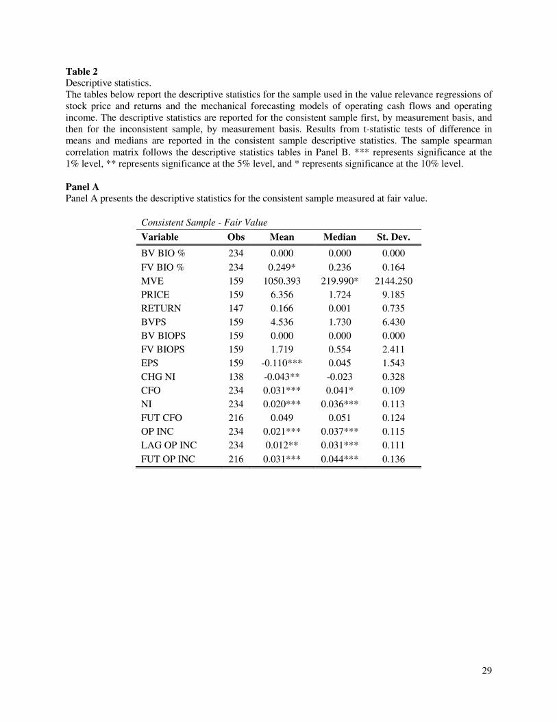
Table 2 provides descriptive statistics for the variables used in the estimations for the consistent and

inconsistent samples, by measurement basis. All data is reported in USD and winsorized at the second

and 98th percentiles to reduce the influence of outliers on results. Panel A (Panel C) provides descriptive

statistics for the consistent (inconsistent) sample with biological assets measured at fair value, while Panel

B (Panel D) provides descriptive statistics for the consistent (inconsistent) sample with biological assets

measured at historical cost. Results from t-statistic tests of differences in means and medians between the

14 My findings are robust to the exclusion of the firm-year observations that pre-date IAS 41.

18

consistent and inconsistent samples by measurement basis are reported in the descriptive statistic tables

for the consistent sample.

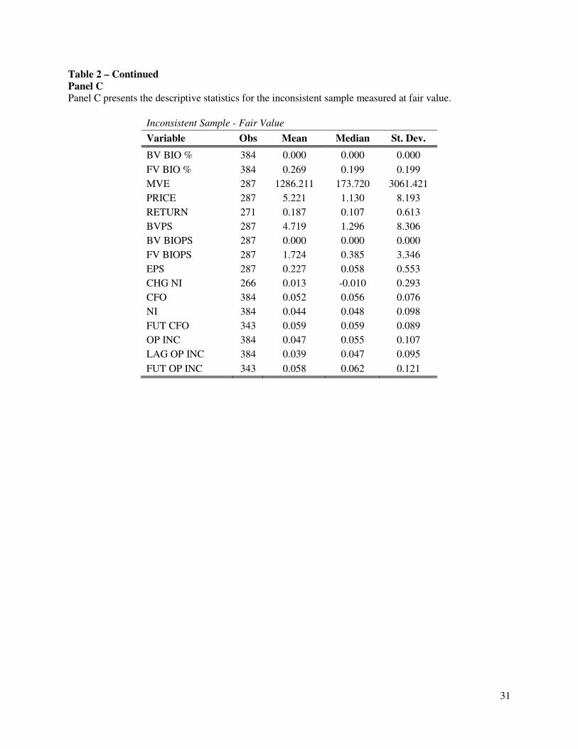
For the sample of firms that measure their biological assets at fair value (Table 2, Panels A and C),

the inconsistent sample holds significantly more biological assets as a percentage of total assets (27% vs

25%). The inconsistent sample is also more profitable than the consistent sample captured by earnings per

share, excluding URGL related to changes in the fair value of the biological assets, ($0.23 vs -$0.11),

operating cash flows ($0.06 vs. $0.03), net income ($0.04 vs. $0.02), operating income ($0.05 vs. $0.02)

and future operating income ($0.06 vs. $0.03). There consistent and inconsistent sample are not

statistically different, however, in terms of market value ($1,050 million vs. $1,286 million), price ($6.36

vs. $5.22) or returns (16.6% vs. 18.7%).

For the sample of firms that measure their biological assets at historical cost (Table 2, Panels B and

D), the inconsistent sample holds significantly more biological assets as a percentage of total assets (27%

vs 21%). The consistent and inconsistent samples are not statistically different on either the price and

return or operating cash flows and income dimensions. On average, earnings per share, excluding URGL,

is $0.08 for the consistent sample and $0.07 for the consistent sample, while average price is $1.36 for the

consistent sample and $1.05 for the inconsistent sample. Overall, the sample of firms that measure their

biological assets at historical cost are smaller, in terms of market value and price, than the sample of firms

that measure their biological assets at fair value.

5. Results

5.1 Price and Return Results

Table 3 Panel A presents the results from the price and return estimations on the full sample.

Column (1) presents the results from the price estimation, while column (2) presents the results from the

return estimation. Consistent with prior value relevance research, both book value and earnings per share

are significantly associated with price. The fair value of the biological assets is significantly associated

with price, but the book value of biological assets is not. Further, for the consistent sample, the fair value

of the biological assets is incrementally more significant. Specifically, the results in column (1) suggest

19

that for the inconsistent sample, for every $1 of biological assets measured at fair value per share, $1.10 is

impounded into price, but for the consistent measurement sample, almost twice as much value is

impounded into price: for every $1 of biological assets measured at fair value $2.01 ($1.10+$0.91) of the

fair value is impounded into price. This suggests that when biological assets are measured consistent with

their use, the value of the biological assets is significantly more value relevant than when measurement is

inconsistent with asset use. Moreover, the return results in column (2) continue to support my main

hypothesis. Specifically, the results in column (2) suggest that only when biological assets are measured

consistent with their use is net income significantly associated with firm returns.

Table 3 Panel B presents the results from the price and return estimations on the sample by

measurement basis. Consistent with the results for the full sample in Panel A, columns (1) and (2) in

Panel B suggest that when measurement is consistent with use, the fair value and book value of the

biological assets are significantly more relevant than when measurement is inconsistent with asset use.

Specifically, column (1) presents the price results for the sample of firms that measure their biological

assets at fair value. The results suggests that when measurement is inconsistent with asset use, only $1.14

of the fair value of the biological assets is impounded into price, while when measurement is consistent

with asset use $1.89 ($1.14+$0.75) of the fair value of the biological assets is impounded into price.

Column (2) presents the price results for the sample of firms that measure their biological assets

at historical cost. The book value of the biological assets is significantly associated with price for the

inconsistent sample, although the coefficient is negative. This result could be driven by the small sample

of firms in the historical cost sample, which may add noise to the coefficient estimates. Nevertheless, the

book value of the biological assets is significantly more relevant when the biological assets are measured

consistent with their use.

Column (3) presents the return results for the fair value sample. Again, consistent with the results

in Panel A for the full sample, net income is incrementally more value relevant when the biological assets

are measured consistent with their use, relative to when they are not. Specifically, the results in column

(3) suggest that when measurement is inconsistent with asset use, $0.52 of net income is impounded into

20

firm returns, but when measurement is consistent with use $0.68 of net income is impounded into price.

In the return estimation for the historical cost sample in column (4), no variables are significantly

associated with firm returns. Again, this result could be driven by the small sample of firms in the

historical cost sample.

Taken together, the price and return results in Panels A and B provide support for my main

hypothesis, namely that asset measurement consistent with asset use provides investors with relatively

more value relevant financial information than measurement that is not linked to asset use.

5.2 Operating Cash Flows and Operating Income Forecasting Results

Table 4, Panel A presents the results from the mechanical forecasting models of future operating

cash flows for the full sample. Column (1) presents the results for future cash flows one period into the

future, while column (2) presents the results for the sum of future operating cash flows one, two and three

periods ahead of fiscal year t.

In both columns (1) and (2), current period operating cash flows are significantly associated with

future cash flows. The results in column (1) suggest, however, that while net income is significantly

predictive of future operating cash flows, it is incrementally more predictive of future operating cash

flows when measurement is consistent with use. Specifically, when measurement is inconsistent with

assets use, $0.14 of net income maps into future operating cash flows, but when measurement is

consistent with asset use, $0.20 more of net income maps into future operating cash flows. Further, the

results in column (2) suggest that net income is predictive of the sum of future operating cash flows one,

two and three periods ahead of the current fiscal year, only when measurement is consistent with use.

When measurement is inconsistent with asset use, net income is not predictive of the sum of future

operating cash flows.

Table 4, Panel B presents the operating cash flows results by measurement basis. Columns (1)

and (2) suggest that when measurement is consistent with asset use, net income is incrementally more

predictive of future operating cash flows, for both the fair value and historical cost samples. Further,

21

columns (3) and (4) suggests that for both the historical cost and fair value samples, net income is

predictive of the sum of future operating cash flows only when measurement is consistent with asset use.

Overall, the operating cash flows results in Table 4 provide support for my hypothesis, that financial

information is more value relevant when measurement is consistent with asset use, relative to when it is

not.

Finally, Table 5, Panel A presents the results from the mechanical forecasting models of future

operating income for the full sample. Column (1) presents the results for future operating income one

period into the future, while column (2) presents the results for future operating income two periods into

the future and column (3) presents the results for future operating income three periods into the future.

Across all time horizons, current period operating income and lagged operating income are significantly

associated with future operating income. Operating income for the consistent sample, however, is

incrementally more predictive of future operating income one period ahead of the current fiscal year. It is

not significantly more predictive of future operating income two and three periods ahead of the current

fiscal year. Panel B presents the results of the mechanical forecasting model of future operating income

by measurement basis. Given the results in Panel A, I only include estimations of future operating income

one period into the future. The results in column (1) suggest that for firms that measure their biological

assets at fair value, operating income is predictive of future operating income only when measurement is

consistent with asset use. The results in column (2) suggest that for firms that measure their biological

assets at historical cost, operating income is incrementally more predictive of future operating income.

Collectively, the results from the mechanical forecasting models of future operating cash flows

and operating income provide support for my hypothesis. Specifically, the results suggest that when

measurement is consistent with the biological assets’ use, net income and operating income are

significantly more predictive of future firm performance.

6. Conclusion

I empirically examine whether asset measurement linked to asset use provides investors with

relatively more value relevant information than when measurement is not linked to asset use. I test a

22

measurement framework proposed by Botosan and Huffman (2013), which predicts that asset

measurement guided by the way in which assets derive value, either in-use or in-exchange, provides

investors with decision-useful information to assess firm value. I test this framework in a sample of 183

firms from 35 different countries that adopt IAS 41. IAS 41 prescribes fair value measurement for

biological assets, which are living plants and animals. Biological assets derive value in-use and in-

exchange. I employ IAS 41’s definition of bearer and consumable biological assets to classify biological

assets as deriving value in-use or in-exchange, respectively. I classify firm-year observations as

measurement consistent with asset use and measurement inconsistent with asset use based on the value

realization of the biological assets, either in-use or in-exchange, and the measurement of the biological

assets, either fair value of historical cost.

I adopt a multi-pronged approach to assess decision-usefulness. First, I examine value relevance

regressions of stock price and returns for the consistent and inconsistent measurement samples. Second, I

examine mechanical forecasting models for operating cash flows and operating income. I find that

measurement consistent with asset use provides investors with relatively more value relevant information

than asset measurement that is inconsistent with asset use. Specifically, I find that firm inputs to price and

return estimations, and mechanical forecasting models of future operating cash flows are significantly

more predictive of future firm performance when biological assets are measured consistent with their use,

relative to when they are not. This finding provides support for early accounting theory that links

decision-useful asset measurement to the way in which the asset generates value (e.g. Littleton 1935; May

1936) and the Botosan and Huffman (2013) framework.

My findings support an asset measurement framework that links asset measurement to asset use, and

suggest that a measurement basis that violates the link to asset use provides investors with relatively less

value relevant information to assess firm value.

23

REFERENCES

Aboody, D., M.E. Barth and R. Kasnik. 1999. “Revaluations of fixed assets and future firm performance: Evidence from the UK.” Journal of Accounting and Economics 26: 149-178.

Ahmed, A.S. and C. Takeda. 1995. “Stock market valuation of gains and losses on commercial banks investment securities: An empirical analysis.” Journal of Accounting and Economics 20: 207- 225.

Ahmed, A.S., E. Kilic, and G.J. Lobo. 2006. “Does recognition versus disclosure matter? Evidence from the value-relevance of banks’ recognized and disclosed derivative financial instruments.” The

Accounting Review 81(3): 567-588. Barth, M.E. 1994a. “Fair Value Accounting: Evidence from investment securities and the market

valuation of banks.” The Accounting Review 69(1): 1-25. Barth, M.E. 1994b. “Fair Value Accounting for banks investment securities: What do bank shares prices

tell us?” Bank Accounting and Finance 7: 13-23. Barth, M.E., M.B. Clement, G. Foster, and R. Kasznik. 1996. “Value-relevance of banks fair value

disclosures under SFAS 107.” The Accounting Review 71:513-537. Barth, M.E. and G. Clinch. 1998. "Revalued Financial, Tangible, and Intangible Assets: Associations with

Share Prices and Non-Market-Based Value Estimates." Journal of Accounting Research 36 (Supplement): 199-233.

Barth, M.E. and W.R. Landsman. 1995. “Fundamental issues related to using fair value accounting for financial reporting.” Accounting Horizons 9(4): 97-107.

Barth, M.E., W.R. Landsman, M. Lang, and C. Williams. 2012. “Are IFRS-based and US GAAP-based accounting amounts comparable?” Journal of Accounting and Economics 54(1): 68-93.

Beaver, W.H. and W.R. Landsman. 1983. Incremental information content of Statement No. 33

disclosures. FASB: Norwalk, CT. Beaver, W.H. and S.G. Ryan. 1985. 'How well do statement no. 33 earnings explain stock returns?'

Financial Analysts Journal 41(5): 66-71. Bernard, V.L. and R. Ruland. 1987. "The incremental information content of historical cost and current

cost income numbers: Time series analyses for 1962-1980." The Accounting Review 62: 707-722. Bernard, V.L., R.C. Merton, and K.G. Palepu. 1995. "Mark-to-market accounting for U.S. banks and

thrifts: Lessons from the Danish experience." Journal of Accounting and Research33:1-32. Botosan, C.A. and A.A. Huffman. 2013. "A Business Valuation Framework for Asset Measurement."

University of Utah Working Paper. Cairns, D., D. Massoudi, R. Taplin and A. Tarca. 2011. "IFRS fair value measurement and accounting

policy choice in the United Kingdom and Australia."The British Accounting Review 43(1): 1-21. Christensen, H. and V. Nikolaev. 2013. "Does Fair Value Accouting for Non-Financial Assets Pass the

Market test?" Review of Accounting Studies Forthcoming.

Daske, H., L. Hail, C. Leuz, and R.S. Verdi. 2008. "Mandatory IFRS reporting around the world: Early evidence on the economic consequences." Journal of Accounting Research 46(5): 1085-1142.

Dechow, P.M., L.A. Myers, and C. Shakespeare. 2012. "Fair value accounting and gains from asset securitizations: A convenient earnings management tool with compensation side-benefits." Journal of Accounting and Economics 49(1-2): 2-25.

Dichev, I.D., J.R. Graham, C.R. Harvey, and S. Rajgopal. 2012. "Earnings quality: Evidence from the field." Working Paper.

Easton, P.D., P.H. Eddey and T.S. Harris. 1993. "An Investigation of Revaluations of Tangible Long-Lived Assets." Journal of Accounting Research 31( Supplement): 1-38.

Easton, P.D., M. McAnally, G. Sommers, and C. Zhang. 2013. Financial Statement Analysis & Valuation

(3rd Edition). Cambridge Business Publishers. Eccher, A., K. Ramesh, and S.R. Thiagarajan. 1996. "Fair value disclosures of bank holding companies."

Journal of Accounting and Economics 22:79-117. Elad, C. and K. Herbohn. 2011. Implementing fair value accounting in the agricultural sector. The

24

Institute of Chartered Accountants of Scotland: Edinburgh. Feltham, G.A. and J.A. Ohlson. 1995. “Valuation and clean surplus accounting for operating and financial

activities.” Contemporary Accounting Research 11(2): 689-731. Financial Accoutning Standards Board. 2006. Preliminary Views on an Improved Conceptual Framework

for Financial Reporting: The Objective of Financial Reportin and Qualitative Characteristics of

Decision-Useful Financial Reporting Information. Financial Accounting Standards Board (FASB). 2012. “Discussion paper: Disclosure framework.”

FASB: Norwalk, CT. Fortgang, C.J. and T.M. Mayer. 1985. "Valuation in Bankruptcy." UCLA Law Review 32

(6): 1061-1133. Hitz, J.M. 2007. “The decision usefulness of fair value accounting – A theoretical perspective.” European

Accounting Review 16(2): 323-362. Hopwood, W. and T. Schaefer. 1989. "Firm-specific responsiveness to input price changes and the

incremental information content in current cost income." The Accounting Review 64: 312-338. Institute of Chartered Accountants in England and Wales (ICAEW). 2010. "Business models in

accounting: The theory of the firm and financial reporting." Information for Better Markets

Initiative Paper. International Accounting Standards Board (IASB). 2008. Exposure draft: An improved conceptual

framework for financial reporting. London, UK: IASB. International Accounting Standards Board (IASB). 2009. International Accounting Standard 41:

Agriculture. London, UK: IASB. International Accounting Standards Board (IASB). 2010. Conceptual Framework for Financial Reporting

2010. London, UK: IASB. International Accounting Standards Board (IASB). 2013a. "Discussion Paper: A Review of the

Conceptual Framework for Financial Reporting." London, UK: IASB. International Accounting Standards Board (IASB). 2013b. Exposure draft: Agriculture: Bearer Plants.

London, UK: IASB. Kolev, K. 2009. "Do investors perceive marking-to-model as marking-to-myth? Early evidence

from FAS 157."Working Paper. KPMG. 2008. IFRS Compared to U.S.GAAP. London, UK: KPMG International Financial Reporting

Group. Littleton, A.C. 1935. "Value or Cost." The Accounting Review 10(3): 269-273. Lobo, G.J. and I.M. Song. 1989. "The incremental information in SFAS No. 33 income disclosures over

historical cost income and its cash and accrual components." The Accounting Review 64: 329- 343.

May, G.O. 1936. “The influence of accounting on the development of the economy.” Journal of

Accountancy 61(1):11-22. Milburn, J.A. 2012. Toward a measurement framework for financial reporting by profit-oriented entities.

Canadian Institute of Chartered Accountants. Muller, K.A., E.J. Riedl, and T. Sellhorn. 2011. "Mandatory fair value accounting and information

asymmetry: Evidence form the European real estate industry." Management Science 57(6): 1138- 1153.

Nelson, K.K. 1996. “Fair Value Accounting for Commercial Banks: An Empirical Analysis of SFAS No. 107.” The Accounting Review 71(2): 161-182.

Nissim, D. and S.H. Penman. 2008. "Principles for the application of fair value accounting." Columbia

Business School Center for Excellence in Accounting and Security Analysis Working Paper.

Petroni, K. and J. Whalen. 1995. "Fair values of equity and debt securities and share prices of property casualty insurance companies." Journal of Risk and Insurance 62: 719-737.

Pownall, G., M. Vulcheva, and X. Wang. 2012. "Increasing liquidity on the global stock exchanges: The structure of Euronext." Working Paper.

Song, C.J., W.B. Thomas, and H. Yi. 2010. “Value Relevance of FAS 157 Fair Value Hierarchy

25

Information and the Impact of Corporate Governance Mechanisms.” The Accounting Review 85(4): 1375-1410.

26

APPENDIX A – Variable definitions and calculations.

Variable Name Definition/Calculation

Basic EPS Basic earnings per share from Capital IQ in fiscal year t.

BV BIO % The book value of biological assets measured at cost scaled by total assets, for the sample of firms that hold biological assets measured at cost, i.e. where FV BIO = 0.

BV BIO PS Book value of the biological assets measured at cost (balance sheet value), per share in fiscal year t.

BVPS Book value of equity excluding the fair value and the book value of the biological assets in fiscal year t. (Total Assets – Book Value of Biological Assets - Fair Value of Biological Assets)-Total Liabilities.

CFO Cash flows from operations in fiscal year t.

CHG NI Change in net income, excluding the URGL, from fiscal year t to fiscal year t-1.

Fut CFO Cash flows from operations in fiscal year t+1.

Fut CFO2 Cash flows from operations in fiscal year t+2.

Fut CFO3 Cash flows from operations in fiscal year t+3.

Fut OPINC Operating income in fiscal year t+1.

Fut OPINC2 Operating income in fiscal year t+2.

Fut OPINC3 Operating income in fiscal year t+3.

FV BIO % The fair value of the biological assets scaled by total assets, for the sample of firms that hold biological assets measured at fair value, i.e. where BV BIO = 0.

FV BIO PS Fair value of the biological assets (balance sheet value), per share in fiscal year t.

NI Net income in fiscal year t excluding any URGL related to the change in the fair value of the biological assets.

OP INC Operating income in fiscal year t. Calculated using Capital IQ variables earnings from continuing operations.

Price Price is calculated for the month following the annual report filing or, alternatively, four months following the firm’s fiscal year end. Price is pulled from the firm’s home country exchange and converted to USD. Data is from Datastream.

Return Cumulated 12-month, raw returns over the fiscal year ending the month following the annual report issuance or alternatively, four months following the firm’s fiscal year end. Returns are calculated on the firm’s home country exchange. Data is from Datastream.

TOT BIO % The book value of the biological assets measured at cost plus the fair value of the biological assets, scaled by total assets.

27

Table 1 Descriptive sample statistics. Panel A reports the sample composition of the consistent and inconsistent samples by value realization and measurement. Cells highlighted in yellow comprise firm-year observations classified in the consistent sample, while the remaining cells comprise firm-year observations classified in the inconsistent sample. Panel B presents the composition of the sample by fiscal year. Panel C presents the composition of the sample by country. Panel A

Sample composition of consistent and inconsistent firm-year observations by biological asset value realization and measurement. Highlighted cells are observations classified in the consistent measurement group.

Measurement

FV HC TOTAL

Value

Realization

IN-USE 384 237 621

42% 26% 68%

IN-EXCH 234 54 288

26% 6% 32%

TOTAL 618 291 909

68% 32% 100%

Panel B

Sample composition of firm-year observations by fiscal year.

FYEAR Observations % of Total

1999 1 0.1%

2000 4 0.4%

2001 10 1.1%

2002 13 1.4%

2003 27 3.0%

2004 40 4.4%

2005 51 5.6%

2006 73 8.0%

2007 89 9.8%

2008 120 13.2%

2009 138 15.2%

2010 137 15.1%

2011 136 15.0%

2012 70 7.7%

TOTAL 909 100.0%

28

Table 1 – Continued

Panel C

Sample composition of firms by country of origin.

Country Firms % of Total Country Firms % of Total

Australia 23 12.6% Mozambique 1 0.5%

Brazil 9 4.9% Netherlands 1 0.5%

Canada 7 3.8% New Zealand 7 3.8%

Channel Islands 2 1.1% Norway 8 4.4%

Chile 4 2.2% Peru 2 1.1%

China 3 1.6% Philippines 4 2.2%

Denmark 1 0.5% Portugal 2 1.1%

Finland 3 1.6% Singapore 12 6.6%

Greece 2 1.1% South Africa 6 3.3%

Hong Kong 9 4.9% Spain 1 0.5%

Indonesia 1 0.5% Sri Lanka 9 4.9%

Jamaica 1 0.5% Sweden 3 1.6%

Latvia 3 1.6% Switzerland 1 0.5%

Lithuania 1 0.5% Turkey 1 0.5%

Luxembourg 2 1.1% Ukraine 3 1.6%

Malaysia 41 22.4% United Kingdom 7 3.8%

Mauritius 1 0.5% Zambia 1 0.5%

Mexico 1 0.5%

TOTAL FIRMS 183 100.0%

29

Table 2 Descriptive statistics. The tables below report the descriptive statistics for the sample used in the value relevance regressions of stock price and returns and the mechanical forecasting models of operating cash flows and operating income. The descriptive statistics are reported for the consistent sample first, by measurement basis, and then for the inconsistent sample, by measurement basis. Results from t-statistic tests of difference in means and medians are reported in the consistent sample descriptive statistics. The sample spearman correlation matrix follows the descriptive statistics tables in Panel B. *** represents significance at the 1% level, ** represents significance at the 5% level, and * represents significance at the 10% level. Panel A Panel A presents the descriptive statistics for the consistent sample measured at fair value.

Consistent Sample - Fair Value

Variable Obs Mean Median St. Dev.

BV BIO % 234 0.000 0.000 0.000

FV BIO % 234 0.249* 0.236 0.164

MVE 159 1050.393 219.990* 2144.250

PRICE 159 6.356 1.724 9.185

RETURN 147 0.166 0.001 0.735

BVPS 159 4.536 1.730 6.430

BV BIOPS 159 0.000 0.000 0.000

FV BIOPS 159 1.719 0.554 2.411

EPS 159 -0.110*** 0.045 1.543

CHG NI 138 -0.043** -0.023 0.328

CFO 234 0.031*** 0.041* 0.109

NI 234 0.020*** 0.036*** 0.113

FUT CFO 216 0.049 0.051 0.124

OP INC 234 0.021*** 0.037*** 0.115

LAG OP INC 234 0.012** 0.031*** 0.111

FUT OP INC 216 0.031*** 0.044*** 0.136

30

Table 2 - Continued

Panel B

Panel B presents the descriptive statistics for the consistent sample measured at historical cost.

Consistent - Historical Cost

Variable Obs Mean Median St. Dev.

BV BIO % 237 0.208*** 0.166 0.145

FV BIO % 237 0.000 0.000 0.000

MVE 199 776.497 88.230 2280.148

PRICE 199 1.360 0.536 3.193

RETURN 195 0.263 0.210** 0.541

BVPS 199 0.821 0.493 1.105

BV BIOPS 199 0.199 0.138*** 0.188

FV BIOPS 199 0.000 0.000 0.000

EPS 199 0.084 0.042** 0.123

CHG NI 197 0.029 0.023 0.198

CFO 237 0.072 0.070 0.077

NI 237 0.047 0.051 0.084

FUT CFO 218 0.086 0.076 0.088

OP INC 237 0.050 0.052 0.087

LAG OP INC 237 0.038 0.047 0.090

FUT OP INC 218 0.064 0.064* 0.097

31

Table 2 – Continued

Panel C

Panel C presents the descriptive statistics for the inconsistent sample measured at fair value.

Inconsistent Sample - Fair Value

Variable Obs Mean Median St. Dev.

BV BIO % 384 0.000 0.000 0.000

FV BIO % 384 0.269 0.199 0.199

MVE 287 1286.211 173.720 3061.421

PRICE 287 5.221 1.130 8.193

RETURN 271 0.187 0.107 0.613

BVPS 287 4.719 1.296 8.306

BV BIOPS 287 0.000 0.000 0.000

FV BIOPS 287 1.724 0.385 3.346

EPS 287 0.227 0.058 0.553

CHG NI 266 0.013 -0.010 0.293

CFO 384 0.052 0.056 0.076

NI 384 0.044 0.048 0.098

FUT CFO 343 0.059 0.059 0.089

OP INC 384 0.047 0.055 0.107

LAG OP INC 384 0.039 0.047 0.095

FUT OP INC 343 0.058 0.062 0.121

32

Table 2 – Continued

Panel D

Panel D presents the descriptive statistics for the inconsistent sample measured at historical cost.

Inconsistent - Historical Cost

Variable Obs Mean Median St. Dev.

BV BIO % 54 0.269 0.186 0.240

FV BIO % 54 0.000 0.000 0.000

MVE 34 206.103 65.420 236.581

PRICE 34 1.046 0.327 2.145

RETURN 32 0.102 -0.140 0.703

BVPS 34 0.865 0.260 1.778

BV BIOPS 34 0.101 0.059 0.079

FV BIOPS 34 0.000 0.000 0.000

EPS 34 0.070 0.011 0.282

CHG NI 32 0.022 0.006 0.099

CFO 54 0.056 0.058 0.095

NI 54 0.018 0.035 0.109

FUT CFO 50 0.066 0.076 0.109

OP INC 54 0.012 0.030 0.101

LAG OP INC 54 0.003 0.034 0.116

FUT OP INC 50 0.024 0.036 0.122

33

Table 2 – Continued

Panel E

Panel E presents the Spearman correlations among the sample variables. Bolded amounts are significant at the 1%, 5% or 10% level.

CON PRICE RETURN BVPS BV BIO

PS

FV BIO

PS EPS CHG NI CFO NI

FUT

CFO

OP

INC

LAG OP

INC

FUT OP

INC

CONSISTENT 1

PRICE -0.1233 1

RETURN 0.0562 0.1411 1

BVPS -0.151 0.9053 0.0108 1

BV BIO PS 0.5019 -0.2072 0.1073 -0.2366 1

FV BIO PS -0.4137 0.6041 -0.0884 0.6638 -0.8259 1

EPS -0.0721 0.5969 0.2122 0.5384 0.0275 0.2129 1

CHG NI 0.0851 -0.0521 0.2882 -0.1071 0.1938 -0.2299 0.336 1

CFO 0.0289 0.3341 0.2494 0.246 0.1891 -0.0264 0.5649 0.2565 1

NI -0.0144 0.2721 0.2967 0.1298 0.1516 -0.0724 0.6316 0.3501 0.5845 1

FUT CFO 0.0623 0.3084 0.2047 0.2113 0.2066 -0.0643 0.4615 0.2291 0.5844 0.509 1

OP INC -0.0174 0.2706 0.2951 0.1334 0.149 -0.0675 0.6278 0.3484 0.5863 0.9888 0.5124 1

LAG OP INC -0.0387 0.2395 -0.026 0.1392 0.1073 -0.0247 0.421 -0.2625 0.4314 0.5769 0.3752 0.5832 1

FUT OP INC 0.0264 0.2395 0.3311 0.0865 0.1879 -0.1237 0.4265 0.2137 0.5235 0.6452 0.6486 0.6549 0.4558 1

34

Table 3 Price and Return Results Table 3 reports the results from the stock price and return estimations. Results for the full sample are reported in Panel A, and results by measurement basis are reported in Panel B. Robust t-statistics, clustered by firm and year, are reported in parentheses below coefficient estimates. Coefficient significance on the interaction terms is determined by a one-tailed test. Price variables are per share. Return variables are scaled by the beginning period market value of equity. See Appendix A for variable definitions. *** represents significance at the 1% level, ** represents significance at the 5% level, and * represents significance at the 10% level. Panel A Price and return results for the full sample.

(1) (2)

VARIABLES Expectations PRICE RETURN

CONSISTENT ? -0.34 0.03***

(-0.81) (5.29)

BVPS + 0.78***

(5.71)

EPS + 1.70***

(3.58)

BV BIO PS + 0.91

(0.26)

FV BIO PS + 1.10***

(4.93)

BV BIO PS * CONSISTENT + 3.41

(0.74)

FV BIO PS * CONSISTENT + 0.91***

(2.46)

NI +

0.11

(0.50)

CHG NI +

0.25*

(1.82)

NI * CONSISTENT +

0.38**

(1.65)

INTERCEPT 0.60* 0.16

(1.92) (1.59)

Observations 679 628

R-squared 0.81 0.04

35

Table 3 – Continued

Panel B

Price and return results by measurement basis.

(1) (2) (3) (4)

FV HC

FV HC

VARIABLES Expectations PRICE PRICE RETURN RETURN

CONSISTENT ? 0.34 -1.08***

-0.00 0.04

(0.60) (-2.90)

(-0.01) (0.39)

BVPS + 0.75*** 1.95***

(5.59) (11.66)

EPS + 1.62*** 3.48*

(3.47) (1.87)

BV BIO PS +

-6.37**

(-2.01)

FV BIO PS + 1.14***

(5.25)

BV BIO PS * CONSISTENT +

9.50***

(2.67)

FV BIO PS * CONSISTENT + 0.75**

(2.00)

NI +

0.14 -0.69

(0.77) (-0.60)

CHG NI +

0.39*** -0.05

(2.67) (-0.14)

NI * CONSISTENT +

0.52** 1.27

(2.01) (1.01)

INTERCEPT

0.68** 0.35

0.16*** 0.17**

(2.07) (1.57)

(3.84) (2.09)

Observations

446 233

402 226

R-squared 0.81 0.72 0.10 0.16

36

Table 4 Operating Cash Flows Results Table 4 reports the results from the mechanical forecasting model for future operating cash flows. Results for the full sample are reported in Panel A, and results by measurement basis are reported in Panel B. Robust t-statistics, clustered by firm, are reported in parentheses below coefficient estimates. Country fixed effects are included in all estimations. Coefficient significance for the interaction terms is determined by a one-tailed test. All variables are scaled by average total assets. See Appendix A for variable definitions. *** represents significance at the 1% level, ** represents significance at the 5% level, and * represents significance at the 10% level. Panel A Operating cash flows results for the full sample.

(1) (2)

VARIABLES Expectations FUT CFO SUM FUT

CFO

CONSISTENT ? 0.004 -0.021

(0.569) (-0.522)

CFO + 0.448*** 1.309***

(6.490) (3.982)

NI + 0.139*** 0.374

(2.848) (1.447)

NI * CONSISTENT + 0.197*** 0.969**

(2.869) (2.165)

INTERCEPT 0.029*** 0.139***

(6.146) (6.517)

Observations 827 536

R-squared 0.450 0.538

Country Fixed Effects Y Y

37

Table 4 – Continued

Panel B

Operating cash flows results by measurement basis.

(1) (2) (3) (4)

FV HC FV HC

VARIABLES Expectations FUT CFO FUT CFO SUM FUT

CFO

SUM FUT

CFO

CONSISTENT ? 0.004 0.022 -0.023 -0.006

(0.316) (1.543) (-0.357) (-0.082)

CFO + 0.507*** 0.278*** 1.647*** 0.612

(5.925) (2.696) (3.813) (1.493)

NI + 0.125** 0.216** 0.360 -0.048

(2.261) (2.127) (1.246) (-0.124)

NI * CONSISTENT + 0.141* 0.285** 0.914* 1.642**

(1.678) (2.029) (1.493) (2.443)

INTERCEPT 0.025*** 0.025* 0.117*** 0.183***

(4.673) (1.895) (4.914) (2.873)

Observations 559 268 353 183

R-squared 0.476 0.389 0.578 0.502

Country Fixed Effects Y Y Y Y

38

Table 5

Operating Income Results Table 5 reports the results from the mechanical forecasting model for operating income. Results for the full sample are reported in Panel A, and results by measurement basis are reported in Panel B. Robust t-statistics, clustered by firm, are reported in parentheses below coefficient estimates. Country fixed effects are included in all estimations. Coefficient significance for the interaction terms is determined by a one-tailed test. All variables are scaled by average total assets. See Appendix A for variable definitions. *** represents significance at the 1% level, ** represents significance at the 5% level, and * represents significance at the 10% level. Panel A Operating income results for the full sample.

(1) (2) (3)

VARIABLES Expectations FUT OP FUT OP2 FUT OP3

CONSISTENT ? -0.008 -0.004 -0.004

(-1.018) (-0.256) (-0.220)

OP INC + 0.563*** 0.348** 0.442**

(7.442) (2.422) (2.273)

LAG OP INC + 0.109* 0.324*** 0.240**

(1.954) (5.004) (2.320)

OP INC * CONSISTENT + 0.202** 0.139 0.045

(2.011) (0.831) (0.190)

INTERCPET 0.025*** 0.035*** 0.047***

(5.128) (3.875) (3.812)

Observations 827 679 536

R-squared 0.513 0.383 0.337

Country Fixed Effects Y Y Y

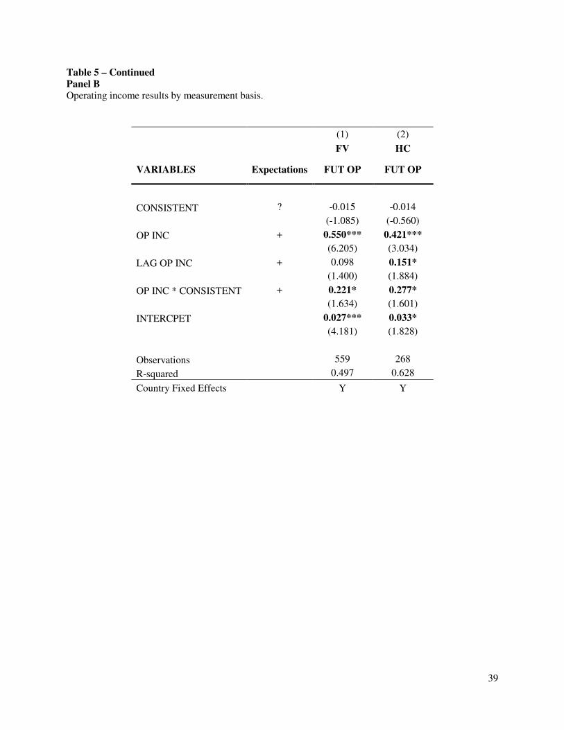
39

Table 5 – Continued

Panel B

Operating income results by measurement basis.

(1) (2)

FV HC

VARIABLES Expectations FUT OP FUT OP

CONSISTENT ? -0.015 -0.014

(-1.085) (-0.560)

OP INC + 0.550*** 0.421***

(6.205) (3.034)

LAG OP INC + 0.098 0.151*

(1.400) (1.884)

OP INC * CONSISTENT + 0.221* 0.277*

(1.634) (1.601)

INTERCPET 0.027*** 0.033*

(4.181) (1.828)

Observations

559 268

R-squared 0.497 0.628

Country Fixed Effects Y Y