Notes Relating to Newton Series for the Riemann Zeta Function

Value-distribution of theRiemann zeta-function and related functions
near the critical line
Dissertationsschrift zur Erlangung des naturwissenschaftlichen
Doktorgrades der Julius-Maximilians-Universität Würzburg
vorgelegt von
Thomas Christ
aus
Ansbach, Deutschland
Würzburg 2013

Eingereicht am 10.12.2013
bei der Fakultät für Mathematik und Informatik
der Julius-Maximilians-Universität Würzburg
1. Gutachter: Prof. Dr. Jörn Steuding
2. Gutachter: Prof. Dr. Ramunas Garunkštis
Tag der Disputation: 22.04.2014

Contents
Notations 1
Acknowledgments 3
Introduction and statement of the main results 5P.1 The Riemann zeta-function . . . . . . . . . . . . . . . . . . . . . . . . . . 5P.2 The Selberg class and the extended Selberg class . . . . . . . . . . . . . . 11P.3 Statement of the main results and outline of the thesis . . . . . . . . . . . 14
I Value-distribution near the critical line 19
1 A Riemann-type functional equation 211.1 The factor ∆p of a Riemann-type functional equation . . . . . . . . . . . . 211.2 The class G . . . . . . . . . . . . . . . . . . . . . . . . . . . . . . . . . . . 24
2 A modified concept of universality near the critical line 292.1 Failure of Voronin’s universality theorem around the critical line . . . . . 292.2 A limiting process in neighbourhoods of the critical line . . . . . . . . . . 302.3 Convergence and non-convergence of the limiting process . . . . . . . . . . 39
2.3.1 Non-convergence of the limiting process . . . . . . . . . . . . . . . 392.3.2 Convergence via the growth behaviour in S# . . . . . . . . . . . . 402.3.3 Convergence via the a-point-distribution in S#
R . . . . . . . . . . . 43
3 Small and Large values near the critical line 473.1 Selberg’s central limit law . . . . . . . . . . . . . . . . . . . . . . . . . . . 473.2 Small and large values on the critical line . . . . . . . . . . . . . . . . . . 493.3 Small and large values near the critical line . . . . . . . . . . . . . . . . . 513.4 Unboundedness on the critical line in the extended Selberg class . . . . . . 56
3.4.1 Characteristic convergence abscissae in the extended Selberg class . 563.4.2 Almost periodicity and a Phragmén-Lindelöf argument . . . . . . . 603.4.3 Mean-square values in the extended Selberg class . . . . . . . . . . 613.4.4 Summary: The quantities αL,inf and αL,sup for L ∈ S# . . . . . . 64
4 a-point-distribution near the critical line 674.1 General results on the a-point-distribution in the extended Selberg class . 684.2 a-points near the critical line - approach via Littlewood’s lemma . . . . . 714.3 a-points near the critical line - approach via normality theory . . . . . . . 75

4.3.1 Filling discs, Julia directions and Julia lines - Basic properties . . . 754.3.2 Julia directions and Julia lines for the Riemann zeta-function . . . 784.3.3 Filling discs induced by a Riemann-type functional equation . . . . 804.3.4 Filling discs induced by Selberg’s central limit law . . . . . . . . . 834.3.5 Filling discs for the Riemann zeta-function via Ω-results for ζ ′(ρa) 85
4.4 Non-trivial a-points to the left of the critical line . . . . . . . . . . . . . . 884.5 Summary: a-points of the Riemann zeta-function near the critical line . . 89
5 Denseness results for the Riemann zeta-function in the critical strip 915.1 The works of Bohr and Voronin . . . . . . . . . . . . . . . . . . . . . . . . 925.2 Qualitative difference of the value-distribution on the critical line . . . . . 955.3 Approaching zero and infinity from different directions . . . . . . . . . . . 975.4 Denseness results on curves approaching the critical line . . . . . . . . . . 995.5 Denseness results on curves approaching the line σ = 1 . . . . . . . . . . . 1045.6 A limiting process to the right of the critical line . . . . . . . . . . . . . . 106
II Discrete and continuous moments 107
6 Arithmetic functions and Dirichlet series coefficients 1116.1 Arithmetic functions connected to the Riemann zeta-function . . . . . . . 1116.2 The coefficients of certain Dirichlet series . . . . . . . . . . . . . . . . . . . 116
7 Dirichlet series and the infinite dimensional torus 1237.1 The infinite dimensional torus, the compact group K and a local product
decomposition of K . . . . . . . . . . . . . . . . . . . . . . . . . . . . . . . 1237.2 An ergodic flow on K and a special version of the ergodic theorem . . . . 1267.3 Extension of Dirichlet series to functions on the infinite dimensional torus 1287.4 The space H 2 of Dirichlet series with square summable coefficients . . . . 131
8 The class N and vertical limit functions 1358.1 The class N and its elements . . . . . . . . . . . . . . . . . . . . . . . . . 1358.2 Normal families related to a function of the class N . . . . . . . . . . . . . 1438.3 The class N and a polynomial Euler product representation . . . . . . . . 1468.4 Vertical limit functions . . . . . . . . . . . . . . . . . . . . . . . . . . . . 149
9 Discrete and continuous moments to the right of the critical line 1519.1 An extension of a theorem due to Tanaka to the class N (u) . . . . . . . . 1519.2 Proof of the main theorem . . . . . . . . . . . . . . . . . . . . . . . . . . . 1579.3 Applications to the value-distribution of the Riemann zeta-function . . . . 170
Appendix: Normal families of meromorphic functions 171
Bibliography 177

Notations
We indicate some of the basic notations that we use in this thesis. Usually, we denote acomplex variable by s = σ + it with real part σ and imaginary part t.
Set of numbers.
N := 1, 2, 3, ..., the set of positive integersN0 := N ∪ 0, the set of non-negative integersP := 2, 3, 5, ..., the set of prime numbersZ := ...,−1, 0, 1, ..., the set of integersQ the set of rational numbersR the set of real numbersR+ the set of positive real numbersR+
0 the set of non-negative real numbersC the set of complex numbers(xn)n := (xn)n∈N := (x1, x2, ...), a sequence of elements xn from a certain set X.
Subsets of the complex plane.
Dr(s0) open disc with radius r > 0 and center s0 ∈ CD := D1(0), unit disc∂Ω the boundary of a domain Ω ⊂ CD := σ + it ∈ C : 0 < σ < 1, t > 0C := C ∪ ∞, the Riemann sphere(xn)n := (xn)n∈N := (x1, x2, ...), a sequence of elements xn from a certain set X.
Classes of functions.
H(Ω) set of functions analytic in a domain Ω ⊂ CM(Ω) set of functions meromorphic in a domain Ω ⊂ CS the Selberg class, defined in Section P.2S# the extended Selberg class, defined in Section P.2S#R a subclass of the extended Selberg class, defined in Section P.2S∗ a subclass of the Selberg class, defined in Section P.2G an extension of S#, defined in Section 1.2N a class of functions, defined in Section 8.1H 2 a space of Dirichlet series, defined in Section 7.4Lpσσσ(K) the Lp space of a compact group K, defined in Section 7.1(xn)n := (xn)n∈N := (x1, x2, ...), a sequence of elements xn from a certain set X.
1

2 Notations
Some further notations.
meas A Lebesgue measure of a measurable set A ⊂ R.#B cardinality of a finite subset B ⊂ R.dens∗J upper density of a subset J ⊂ N, defined in Section 7.2dens∗J lower density of a subset J ⊂ N, defined in Section 7.2(xn)n := (xn)n∈N := (x1, x2, ...), a sequence of elements xn from a certain set Xn|m n is a divisor of m
Landau’s O-notation and the Vinogradov symbols.
We use Landau’s O-notation and the Vinogradov symbols in the following way. Let fand g be real valued functions, which are both defined on a subset of the reals.
f(x) = O(g(x)
)or f(x) g(x),as x→∞
:⇐⇒ ∃C>0 s.t. lim supx→∞
∣∣∣∣f(x)
g(x)
∣∣∣∣ ≤ Cf(x) = o(g(x)),as x→∞ :⇐⇒ lim sup
x→∞
∣∣∣∣f(x)
g(x)
∣∣∣∣ = 0
f(x) = Ω(g(x)
)or f(x) g(x),as x→∞
:⇐⇒ ∃C>0 s.t. lim supx→∞
∣∣∣∣f(x)
g(x)
∣∣∣∣ ≥ Cf(x) ∼ g(x),as x→∞ :⇐⇒ lim
x→∞
∣∣∣∣f(x)
g(x)
∣∣∣∣ = 1
f(x) g(x),as x→∞ :⇐⇒ ∃A,B>0 s.t. lim inf
x→∞
∣∣∣∣f(x)
g(x)
∣∣∣∣ ≥ A and lim supx→∞
∣∣∣∣f(x)
g(x)
∣∣∣∣ ≤ BSometimes we write Oα(·), resp. α, and Ωα(·), resp. α, to indicate that the impliedconstants depend on the parameter α, respectively.

Acknowledgments
First and foremost, I would like to express my deepest gratitude to my supervisor JörnSteuding. I am grateful for his tremendous support and insightful guidance during thelast years without which this thesis would not have been completed. I appreciated thefriendly and uncomplicated atmosphere in our working group and wish to thank forinvolving me into the academic and scientific life in such a marvelous way.
I would like to give my special thanks to Antanas Laurinčikas, Ramunas Garunkštis andJustas Kalpokas from Vilnius university for fruitful collaborations and their warm andkind hospitality during my stay in Vilnius in 2011.
From April 2011 to September 2013, my work was supported by a scholarship of theHanns-Seidel-Stiftung funded by the German Federal Ministry of Education and Research(BMBF). I wish to thank the Hanns-Seidel-Stiftung for their ideational and financialsupport.
I am grateful for the various positions that I could have at the Department of Mathe-matics in Würzburg during my doctorate studies. I would like to thank the members ofchair IV and many other people from the department for their friendship, the inspiringdiscussions and the nice atmosphere at the department.
Last but not least, I owe a great debt of gratitude to my family and my dear friends fortheir enduring support and many unforgettable moments.
Würzburg, December 2013Thomas Christ
3


Introduction and statement of themain results
The Riemann zeta-function is a central object in multiplicative number theory. Itsvalue-distribution in the complex plane encodes deep arithmetic properties of the primenumbers. In fact, many important insights into the distribution of the primes wererevealed by exploring the analytic behaviour of the Riemann zeta-function.
The value-distribution of the Riemann zeta-function, however, is far from being well-understood and bears many interesting analytic phenomena which are worth to be stud-ied, independently of their arithmetical relevance. A crucial role is assigned to theanalytic behaviour of the zeta-function on the so called critical line. The latter formsthe background for several open conjectures; for example, the Riemann hypothesis, theLindelöf hypothesis and Ramachandra’s denseness conjecture.
The scope of this thesis is to understand the behaviour of the Riemann zeta-functionnear and on the critical line in a better way.
In Section P.1 of this introductory chapter, we introduce the Riemann zeta-function andexpose the exceptional character of its behaviour on the critical line.
To figure out which basic features of the Riemann zeta-function are responsible for certainphenomena in its value-distribution, it is reasonable to investigate the zeta-function in abroader context. In Section P.2, we consider the Selberg class, which was introduced bySelberg [171] as a promising attempt to gather all Dirichlet series which satisfy similarproperties as the Riemann zeta-function.
In Section P.3, we provide an outline of this thesis, state the main results and brieflyreport on our methods.
P.1 The Riemann zeta-function
In the following, let s = σ+ it denote a complex variable with real part σ and imaginarypart t. In the half-plane σ > 1, the Riemann zeta-function is defined by an absolutelyconvergent Dirichlet series
ζ(s) :=∞∑n=1
1
ns.
5

6 Introduction and statement of the main result
Euler revealed an intimate connection of ζ(s) to the prime numbers. He discovered thatζ(s) can be rewritten as an infinite product
ζ(s) =∏p∈P
(1− p−s)−1, σ > 1,
where P denotes the set of prime numbers.
In his seminal paper of 1859, Riemann [158] laid the foundations to investigate ζ(s) as afunction of a complex variable s. He discovered that ζ(s) can be continued analyticallyto the whole complex plane, except for a simple pole at s = 1 with residue 1, and satisfiesthe functional equation
(P.1) ζ(s) = ∆(s)ζ(1− s) with ∆(s) = πs−12
Γ(
1−s2
)Γ(s2
) ,
where Γ denotes the Gamma-function. Stirling’s formula allows to describe the analyticbehaviour of the factor ∆(s) appearing in the functional equation in a rather precise way.As |t| → ∞, the asymptotic formula
(P.2) ∆(σ + it) =
( |t|2π
) 12−σ−it
exp(i(t+ π
4 ))
(1 +O(|t|−1))
holds uniformly for σ from an arbitrary bounded interval. The reflection principle
ζ(s) = ζ(s) for s ∈ C
provides a further functional equation for the Riemann zeta-function. Due to the latter,it is sufficient to study the value-distribution of the zeta-function in the upper half-planet ≥ 0.
The functional equation (P.1), together with the reflection principle, evokes a strongsymmetry of the Riemann zeta-function with respect to the so called critical line σ = 1
2 .On the latter, the value-distribution of the Riemann zeta-function is exceptional in manyways.
Zeros of the Riemann zeta-function. The zeta-function has simple zeros at thenegative even integers s = −2n, n ∈ N. These zeros are called trivial zeros. All otherzeros lie inside the so called critical strip 0 ≤ σ ≤ 1. We denote these zeros by ρ =β+ iγ and call them non-trivial zeros. Due to the functional equation and the reflectionprinciple, the non-trivial zeros are symmetrically distributed with respect to the criticalline and the real axis. According to the Riemann-von Mangoldt formula, the numberN(T ) of non-trivial zeros with imaginary part γ ∈ (0, T ] is asymptotically given by
N(T ) =T
2πlog
T
2πe+O(log T ),
as T → ∞. The Riemann hypothesis (RH) states that all non-trivial zeros of theRiemann zeta-function lie on the critical line σ = 1
2 ; or, equivalently, that ζ(s) 6= 0 forσ > 1
2 . The Riemann hypothesis is neither proven nor disproven and is considered asa central open problem in number theory. Its arithmetic relevance lies in the impact ofthe non-trivial zeros on the error term in the prime number theorem. The fact that theRiemann zeta-function is non-vanishing in the half-plane σ ≥ 1 leads to an asymptoticformula for the number π(x) of primes p ∈ P with p ≤ x. Building on ideas of Riemann,

Introduction and statement of the main result 7
this was proved by Hadamard [64] and de La Vallée-Poussin [184], independently. Azero-free region of the Riemann zeta-function to the left of σ = 1 is needed in orderto get an asymptotic formula for π(x) with explicit error term. Up to now, the largestknown zero-free region is due to Korobov [107] and Vinogradov [185]. They showedindependently that, for sufficiently large |t|, the Riemann zeta-function has no zeros inthe region defined by
σ ≥ 1− A
(log |t|) 13 (log log |t|) 2
3
with some constant A > 0. Their result implies that
E(x) := π(x)−∫ x
2
dulog u
x exp
(−B (log x)
35
(log log x)15
)
with some constant B > 0. So far, it is not known whether there exists a θ ∈ [12 , 1)
such that the zeta-function has no zeros in the half-plane σ > θ. Von Koch [106] showedthat E(x) xθ+ε holds, with any ε > 0, if and only if the Riemann zeta-function isnon-vanishing in σ > θ. Thus, in particular, the truth of the Riemann hypothesis wouldimply that E(x) x
12
+ε.
There are some partial results supporting the Riemann hypothesis. Hardy [65] showedthat there are infinitely many zeros on the critical line. His result was improved signif-icantly by Selberg [167] who obtained that a positive proportion of all non-trivial zeroscan be located on the critical line: let N0(T ) denote the number of non-trivial zeroswhich lie on the critical line and have imaginary part γ ∈ (0, T ], then
U := lim infT→∞
N0(T )
N(T )≥ C
with some (computable but very small) constant C > 0. Selberg’s lower bound for U wasimproved considerably by Levinson [116] who obtained that U ≥ 0.3437. Later, Conrey[40] found that U ≥ 0.4088 and, very recently, Bui, Conrey & Young [27] establishedU ≥ 0.4105.
Besides of measuring the number of zeros on the critical line, there are also attempts tobound the number of possible zeros off the critical line. Let N(σ, T ) denote the numberof non-trivial zeros with real part β > σ and imaginary part γ ∈ (0, T ]. Due to a classicalresult of Selberg [168] we know that, uniformly for 1
2 ≤ σ ≤ 1,
(P.3) N(σ, T ) T 1− 14
(σ− 12
) log T.1
Many computer experiments were done in order to find a counterexample for the Riemannhypothesis. However, until now no zero off the critical line was dedected. By usingthe Odlyzko and Schönhage algorithm, Gourdon [61] located the first 1013 zeros of theRiemann zeta-function on the critical line.
According to the simplicity hypothesis, one expects that all zeros of the Riemannzeta-function are simple. Indeed, no multiple zero has been found so far. It is known
1For more advanced zero-density estimates for the Riemann zeta-function the reader is referred toTitchmarsh [182, §9] and Ivić [87, Chapt. 11].
8 Introduction and statement of the main result
that at least a positive proportion of all zeros are simple. Let N∗(T ) denote the numberof simple non-trivial zeros with imaginary part γ ∈ (0, T ]. Levinson [116] proved that
S := lim infT→∞
N∗(T )
N(T )≥ 1
3 .
Bui, Conrey & Young [27] obtained that, unconditionally, S ≥ 0.4058. Very recently,Bui & Heath-Brown [28] proved that S ≥ 19
27 , under the assumption of the Riemannhypothesis.2
Whereas the Riemann hypothesis deals with the horizontal distribution of the non-trivialzeros, there are also many open questions concerning the vertical distribution. Let (γn)ndenote the sequence of all positive imaginary parts of non-trivial zeros in ascending order.Littlewood [119] showed that the gap between two consecutive ordinates γn, γn+1 tendsto zero, as n→∞. In particular, he obtained that, as n→∞,
γn+1 − γn 1
log log log γn.
According to the Riemann-von Mangoldt formula the average spacing between two con-secutive ordinates γn, γn+1 ∈ (T, 2T ] is given by 2π
log T , as T →∞. The gap conjecturepredicts that there appear arbitrarily small and arbitrarily large deviations from theaverage spacing: let
λ := lim supn→∞
(γn+1 − γn) log γn2π
and µ := lim infn→∞
(γn+1 − γn) log γn2π
.
Then, one expects that λ =∞ and µ = 0. It was remarked by Selberg [170] and provedby Fujii [51] that λ > 1 and µ < 1. These are still the only unconditional bounds forλ and µ which are at our disposal. On the assumption of the Riemann hypothesis, thecurrent records in bounding λ and µ are λ > 2.766, according to Bredberg [25], andµ < 0.5154, according to Feng & Wu [50].3
Montgomery [141] studied the pair correlation of ordinates γ, γ′ of non-trivial zeros. Hisinvestigations led him to the conjecture that, for any fixed 0 < α < β,
limT→∞
1
N(T )#
γ, γ′ ∈ (0, T ] : α ≤ (γ − γ′) log T
2π≤ β
=
∫ β
α
(1−
(sinπu
πu
)2)
du.
This is known as Montgomery’s pair correlation conjecture (PCC). The truth ofthe PCC implies that S = 1 and µ = 0. Dyson pointed out to Montgomery that eigen-values of random Hermitian matrices have exactly the same pair correlation function.This observation laid the foundation for many models for the Riemann zeta-function onthe critical line by random matrix theory.
a-points of the Riemann zeta-function. Besides the zeros, it is reasonable to studythe general distribution of the roots of the equation ζ(s) = a, where a is an arbitrarily
2By assuming additionally the truth of the generalized Lindelöf hypothesis, this was already knownto Bui, Conrey & Young [27]. Bui & Heath-Brown [28] succeeded to remove the generalized Lindelöfhypothesis by making careful use of the generalized Vaughan identity.
3If one is willing to assume additional conjectures, there are better results available. By assumingthe generalized Riemann hypothesis, Bui [26] obtained that λ > 3.033. By assuming the Riemannhypothesis and certain moment conjectures originating from random matrix theory, Steuding & Steuding[176] showed that λ =∞, as predicted by the gap conjecture.

Introduction and statement of the main result 9
fixed complex number. We call these roots a-points and denote them by ρa = βa + iγa.For sufficiently large n ∈ N, there is an a-point near every trivial zero s = −2n. Apartfrom these a-points generated by the trivial zeros, there are only finitely many a-pointsin the half-plane σ ≤ 0. We refer to the a-points in σ ≤ 0 as trivial a-points and call allother a-points non-trivial a-points. The non-trivial a-points can be located in a verticalstrip 0 ≤ σ ≤ Ra with a certain real number Ra ≥ 1. In analogy to the case a = 0,Landau [23] established a Riemann-von Mangoldt-type formula for the number Na(T )of non-trivial a-points with imaginary part γa ∈ (0, T ]: as T →∞,
Na(T ) =T
2πlog
T
2πeca+O (log T )
with ca = 1 if a 6= 1 and c1 = 2. Levinson [118] proved that all but O(Na(T )/ log log T )of the a-points with imaginary part γa ∈ (T, 2T ] lie in the strip
(P.4)1
2− (log log T )2
log T< σ <
1
2+
(log log T )2
log T.
Thus, almost all a-points are arbitrarily close to the critical line. Under the assumptionof the RH, this phenomenon was already known to Landau [23]. For a 6= 0, Bohr &Jessen [22] showed that the number Na(σ1, σ2, T ) of non-trivial a-values which lie insidethe strip σ1 < σ < σ2 with arbitrarily chosen 1
2 < σ1 < σ2 < 1 and have imaginary partγa ∈ (0, T ] is given asymptotically by
Na(σ1, σ2, T ) ∼ cT,
as T →∞, with a constant c > 0 that depends on σ1, σ2 and a.
Voronin’s universality theorem. Building on works of Bohr [15, 21, 22] and his col-laborators, Voronin [187] discovered a remarkable universality property of the Riemannzeta-function which states, roughly speaking, that every analytic, non-vanishing functionon a compact set with connected complement inside the strip 1
2 < σ < 1 can be approx-imated by vertical shifts of the Riemann zeta-function. Voronin’s universality theoremwas generalized by Bagchi [4], Reich [154] and others. In its strongest formulation it canbe stated as follows.
Theorem P.1 (Voronin’s universality theorem). Let K be a compact set in the strip12 < σ < 1 with connected complement. Let g be a continuous, non-vanishing functionon K, which is analytic in the interior of K. Then, for every ε > 0,
lim infT→∞
1
Tmeas
τ ∈ (0, T ] : max
s∈K|ζ(s+ iτ)− g(s)| < ε
> 0.
Here and in the following, meas X denotes the Lebesgue measure of a measurable setX ⊂ R. Bagchi [4] discovered that the Riemann hypothesis can be rephrased in termsof universality. The RH is true, if and only if, the zeta-function is recurrent, i.e., ifthe zeta-function can approximate itself in the sense of Voronin’s universality theorem.The RH is true if and only if, for any compact subset K of 1
2 < σ < 1 with connectedcomplement and any ε > 0,
lim infT→∞
1
Tmeas
τ ∈ (0, T ] : max
s∈K|ζ(s+ iτ)− ζ(s)| < ε
> 0.

10 Introduction and statement of the main result
As a direct consequence, the universality theorem implies the following denseness state-ment. For every 1
2 < σ < 1 and n ∈ N0, the set
Vn(σ) := (ζ(σ + it), ζ ′(σ + it), ..., ζ(n)(σ + it)) : t ∈ [0,∞)
lies dense in Cn+1. For n = 0, this was already known to Bohr et. al [15, 21, 22]. Itfollows basically from the Dirichlet representation and the functional equation that, forσ < 0 or σ > 1,
V0(σ) 6= C.
On the assumption of the Riemann hypothesis, Garunkštis & Steuding [54] proved that,for σ < 1
2 ,V0(σ) 6= C.
However, even by assuming the truth of the Riemann hypothesis, it is not known whetherthe values of the zeta-function on the critical line lie dense in C or not. According toRamachandra’s denseness conjecture, we expect that
V0(12) = C.
By assuming several moment conjectures arising from random matrix theory modelsfor the Riemann zeta-function, Kowalski & Nikeghbali [108] obtained that V0(1
2) = C.Garunkštis & Steuding [54] showed that a multidimensional denseness statement for thezeta-function on the critical line does not hold. In particular, they proved that
V1(12) 6= C2.
Mean-square value on vertical lines. An essential ingredient in the proof of Bohr’sdenseness result and Voronin’s universality theorem is the fact that
limT→∞
1
T
∫ T
−T|ζ(σ + it)|2 dt =
∞∑n=1
n−2σ <∞ for σ > 12 .
On the critical line, the methods of Bohr and Voronin collaps, since
1
T
∫ T
−T
∣∣ζ(12 + it)
∣∣2 dt ∼ log T, as T →∞,
according to Hardy & Littlewood [71].
Selberg’s central limit law. Due to Selberg (unpublished), the values of the Riemannzeta-function are Gaussian normally distributed, after some suitable normalization: forany measurable set B ⊂ C with positive Jordan content, as T →∞,
1
Tmeas
t ∈ (0, T ] :log ζ
(12 + it
)√12 log log T
∈ B
∼ 1
2π
∫∫B
exp(−1
2(x2 + y2))dx dy.
For a first published proof, we refer to Joyner [91]. Note that f(x, y) := exp(−1
2(x2 + y2))
defines the density function of the bivariate Gaussian normal distribution.
Growth behaviour of the Riemann zeta-function The Riemann zeta-function is afunction of finite order. For σ ∈ R and any ε > 0,
ζ(σ + it) tθζ(σ)+ε, as |t| → ∞,

Introduction and statement of the main result 11
where θζ(σ) is a continuous, convex function in σ with
θζ(σ) =
0 if σ ≥ 1,12 − σ if σ ≤ 0.
According to the Lindelöf hypothesis (LH), we expect that θζ(12) = 0. This would
imply that
θζ(σ) =
0 if σ ≥ 1
2 ,12 − σ if σ < 1
2 .
However, the Lindelöf hypothesis is neither proven nor disproven. The best known upperbound for θζ(1
2) is due to Huxley [84, 85]. He proved that
θζ(12) ≤ 32
205= 0.1560... .
The truth of the Riemann hypothesis implies the truth of the Lindelöf hypothesis. TheLindelöf hypothesis can be reformulated in terms of power moments to the right of thecritical line. Due to classical works of Hardy & Littlewood [69], the Lindelöf hypothesisis true if and only if, for every k ∈ N and every σ > 1
2 ,
(P.5) limT→∞
1
T
∫ T
1|ζ(σ + it)|2k dt =
∞∑n=1
dk(n)2
n2σ,
where dk denotes the generalized divisor function appearing in the Dirichlet series ex-pansion of ζk. The latter formula is proved only in the cases k = 1, 2 by works of Hardy& Littlewood [68] and Ingham [86].
P.2 The Selberg class and the extended Selberg class
Selberg [171] made a promising attempt to describe axiomatically the class of all Dirichletseries for which an analogue of the Riemann hypothesis is expected to be true.
Definition of the Selberg class. A function L belongs to the Selberg class S if itsatisfies the following properties:
(S.1) Dirichlet series representation. In the half-plane σ > 1, L is given by an absolutelyconvergent Dirichlet series
L(s) =
∞∑n=1
a(n)
ns
with coefficients a(n) ∈ C.
(S.2) Ramanujan hypothesis. The Dirichlet series coefficients of L satisfy the growthcondition a(n) nε for any ε > 0, as n → ∞; here, the implicit constant in theVinogradov symbol may depend on ε.
(S.3) Euler product representation. In the half-plane σ > 1, L has a product representa-tion
L(s) =∏p∈PLp(s),

12 Introduction and statement of the main result
where the product is taken over all prime numbers and
Lp(s) := exp
( ∞∑k=1
b(pk)
pks
)
with suitable coefficients b(pk) ∈ C satisfying b(pk) pkθ with some θ < 12 .
(S.4) Analytic continuation. There exists a non-negative integer k such that (s−1)kL(s)defines an entire function of finite oder.
(S.5) Riemann-type functional equation. L satisfies a functional equation
L(s) = ∆L(s)L(1− s),
where
∆L(s) := ωQ1−2sf∏j=1
Γ (λj(1− s) + µj)
Γ (λjs+ µj),
with positive real numbers Q,λ1, ..., λf and complex numbers µ1, ..., µf , ω withRe µj ≥ 0 and |ω| = 1.
For a concise survey on the Selberg class and a motivation for the choice of the axioms,the reader is referred to Perelli [149].
An important parameter of a function L ∈ S is its so called degree which is defined by
dL := 2
f∑j=1
λj
via the quantities λj from the Riemann-type functional equation. The degree of L ∈ Sis uniquely determined. The Riemann zeta-function is an element of the Selberg class ofdegree one. Its k-th power (k ∈ N) lies also in S and has degree k.
Besides the Riemann zeta-function, the Selberg class contains many other arithmeticalrelevant L-functions. Prominent examples of functions in S are Dirichlet L-functionsattached to primitive characters, Dedekind zeta-functions, Hecke L-functions associatedto algebraic number fields and, under appropriate normalizations, Hecke L-functionsassociated to certain modular forms.
The Euler product representation of these examples has a very special form:
(S.3∗) Polynomial Euler product representation. There exist an integer m ∈ N andα1(p), ..., αm(p) ∈ C such that
L(s) =∏p∈P
m∏j=1
(1− αj(p)
ps
)−1
in the half-plane σ > 1.
In the value-distribution of functions in the Selberg class, there appear similar phenom-ena as in the case of the Riemann zeta-function. It follows from the Euler productrepresentation that L ∈ S has no zeros in the half-plane σ > 1. The function L has zeros

Introduction and statement of the main result 13
which are generated by the poles of the Γ-factors appearing the functional equation.These zeros are called trivial zeros of L and are located at the points
s = −µj + k
λj, k ∈ N0, j = 1, ..., f
All other zeros of L are said to be non-trivial zeros. According to the Grand Riemannhypothesis, one expects that every function L ∈ S satisfies an analogue of the Riemannhypothesis, i.e. the non-trivial zeros of every function L ∈ S are located on the criticalline σ = 1
2 . For general functions in S much less is known than for the special case of theRiemann zeta-function. For example, by now, it is not verified whether every functionL ∈ S satisfies the following zero-density estimate:
(DH) Selberg’s zero-density estimate. Let L ∈ S and N0(σ, T ) denote the number of non-trivial zeros ρ = β + iγ of L with real part β > σ and imaginary part γ ∈ (0, T ].Then, there exists a positive number α such that
N0(σ, T ) T 1−α(σ− 12
) log T
uniformly in σ > 12 , as T →∞.
The Grand density hypothesis asserts that (DH) is true for every L ∈ S. Besides theRiemann zeta-function, (DH) is verified for example for Dirichlet L-functions attachedto primitive characters; see Selberg [169]. Certainly, the truth of the Grand Riemannhypothesis implies the truth of the Grand density hypothesis. Moreover, according to theGrand Lindelöf hypothesis we expect that every function L ∈ S satisfies an analogueof the Lindelöf hypothesis, i.e., for any ε > 0,
L(
12 + it
) tε, as t→∞.
Besides many unsolved analytic questions concerning functions in S, there are also severalstructural problems related to S as a class of Dirichlet series. For example, one expectsthat the Dirichlet series coefficients a(n) of L ∈ S satisfy the following prime mean-squarecondition; see Steuding [175, Chapt. 6.6]:
(S.6) Prime mean-square condition. For L ∈ S, there exist a positive constant κL suchthat
limx→∞
1
π(x)
∑p≤x|a(p)|2 = κL,
here, the summation is taken over all primes p ≤ x.
Selberg [171] conjectured that the Dirichlet series coefficients a(n) of any function L ∈ Ssatisfy the following property:
(S.6∗) Selberg’s prime coefficient condition. For L ∈ S, there exists a positive integer nLsuch that ∑
p∈Pp≤x
|a(p)|2p
= nL log log x+O(1),
as x→∞.

14 Introduction and statement of the main result
We know that the Riemann zeta-function and Dirichlet L-functions attached to primitivecharacters satisfy (S.6) and (S.6∗); see Mertens [131] and Dirichlet [48]. The conditions(S.6) and (S.6∗) are closely related to one another; see Steuding [175, Chapt. 6.6] fordetails. Selberg conjectured that (S.6∗) results from a deeper structure in S: obviously,the Selberg class is multiplicatively closed. We call a function L ∈ S primitive if
L = L1 · L2 with L1,L2 ∈ S
implies that L1 = L or L2 = L. Roughly speaking, primitive functions L ∈ S cannotbe written as a non-trivial product of other functions in S. According to Selberg’sorthogonality conjecture , we expect that the following is true.
(S.6∗∗) Selberg’s orthogonality conjecture. For any primitive functions L1,L2 ∈ S withDirichlet series coefficients aL1(n), resp. aL2(n),
∑p∈Pp≤x
aL1(p)aL2(p)
p=
log log x+O(1) if L1 = L2,
O(1) otherwise.
Besides the Selberg class, we shall also work with certain subclasses or extensions of theSelberg class:
The extended Selberg class S#. A function L 6≡ 0 belongs to the extended Selbergclass S# if it satisfies axioms (S.1), (S.4) and (S.5). The functions in S# do not ne-cessarily satisfy the Riemann hypothesis. The Davenport-Heilbronn zeta-function is anelement of S#, but not of S and has non-trivial zeros off the critical line. However, oneexpects that the Lindelöf hypothesis remains still true for every function L ∈ S#.
The class S#R . A function L ∈ S# with dL > 0 belongs to the class S#
R if it satisfiesadditionally the Ramanujan hypothesis (S.2).
The class S∗. A function L ∈ S belongs to the class S∗ if L satisfies the zero-densityestimate (DH) and Selberg’s prime coefficient condition (S.6∗). One expects that bothconditions hold for every function L ∈ S and, thus, that S∗ = S. We know that theRiemann zeta-function and Dirichlet L-functions attached to primitive characters areelements of S∗.
P.3 Statement of the main results and outline of the thesis
This thesis is divided into two parts. In part I we study the value-distribution of theRiemann zeta-function on and near the critical line. In particular, we focus on thecollapse of the Voronin-type universality property at the critical line and the clusteringof a-points around the critical line. We discuss the interplay of these two features andtheir connection to Ramachandra’s denseness conjecture. In our argumentation, we shalluse several results from the theory of normal families of meromorphic functions. For theconvenience of the reader we summarize the results which we shall need in the appendix.
The critical line is a natural boundary for the Voronin-type universality property of theRiemann zeta-function; see Section 2.1. In Chapter 2 we modify Voronin’s universality

Introduction and statement of the main result 15
12 − λ(τ) + iτ
Re(s)
Im(s)
0
2
112
12 + λ(τ) + iτ
Figure 1: The funnel-shaped region Sλ attached to a certain positive function λ withlimt→∞ λ(t) = 0.
concept. Roughly speaking, we add a scaling factor to the vertical shifts that appear inVoronin’s universality theorem and regard
ζτ (s) := ζ(
12 + λ(τ)s+ iτ
), s ∈ D,
with τ ∈ [2,∞) and a positive function λ satisfying limτ→∞ λ(τ) = 0. By sending τ toinfinity, this leads to a limiting process for the Riemann zeta-function in a funnel-shapedneighbourhood of the critical line, more precisely in the region
Sλ :=σ + it ∈ C : 1
2 − λ(t) < σ < 12 + λ(t), t ≥ 2
.
We shall see in Proposition 2.1 that possible limit functions of this process depend onthe choice of λ and are strongly affected by the functional equation of the Riemannzeta-function. Our results do not only apply for the Riemann zeta-function but hold formeromorphic functions that satisfy a Riemann-type functional equation in general. Forthis purpose, we define in Chapter 1 the class G, which generalizes the extended Selbergclass S#.
In Chapter 3 we shall see that Selberg’s central limit law implies that, for suitablychosen λ, the limiting process of Chapter 2 has a strong tendency to converge to g ≡ 0or to g ≡ ∞; see Theorem 3.2. This provides information on the frequency of smalland large values of the Riemann zeta-function in certain regions Sλ and complementsrecults of Laurinčikas [111, Chapt. 3, Theorem 3.5.1], Bourgade [24] and others whoestablished certain extensions of Selberg’s central limit law; see Section 3.1. For example,we deduce that the Riemann zeta-function assumes both arbitrarily small and arbitrarilylarge values on every path to infinity which lies inside Sλ, where the function λ satisfies
λ(t) =c
log t, t ≥ 2,
with an arbitrary constant c > 0; see Corollary 3.3 and Corollary 5.11. Selberg’s centrallimit law does not only apply to the Riemann zeta-function. Due to Selberg [171] it holds

16 Introduction and statement of the main result
(with suitable adaptions) for every function in the class S∗. Thus, most of our results inChapter 3 hold for arbitrary functions L ∈ S∗.
Levinson [118] showed that the a-points of the Riemann zeta-function cluster around thecritical line. In Chapter 4 we investigate how to choose λ such that almost all or infinitelymany a-points of the Riemann zeta-function lie in the region Sλ. Levinson [118] reliedessentially on a lemma of Littlewood which can be considered as an integrated versionof the principle of argument. Endowed with a result of Selberg [171], resp. Tsang [183,§8], Levinson’s method yields that, for any a ∈ C, almost all a-points of the Riemannzeta-function (in a certain density sense) lie inside the region Sλ, if λ is chosen such that
λ(t) =µ(t)√
log log t
log t, t ≥ 2,
with an arbitrary positive function µ satisfying limt→∞ µ(t) = ∞; see Theorem 4.7.Besides Levinson’s method, we use certain arguments from the theory of normal familiesand rely on the notation of filling discs to study the a-point distribution of the Riemannzeta-function near the critical line. With these concepts we obtain new insights into thea-point distribution, complementing the observations of Levinson. In particular, we showthat, for every a ∈ C, with at most one exception, there are infinitely many a-points ofthe Riemann zeta-function inside the region Sλ, if λ is chosen such that
λ(t) =µ(t)
log t, t ≥ 2,
with any positive function µ satisfying limt→∞ µ(t) =∞; see Theorem 4.7. We shall seethat, under quite general assumptions, the same is true for functions in G. Beyond this,relying on a result of Ng [147], we prove that, under the assumption of the generalizedRiemann hypothesis for Dirichlet L-functions, for every a ∈ C, with at most one excep-tion, there are infinitely many a-points of the Riemann zeta-function inside the regionSλ, if λ satisfies
λ(t) = µ(t) exp
(−c0
log t
log log t
), t ≥ 2,
where µ is any positive function satisfying limt→∞ µ(t) =∞ and c0 any positive constantless than 1√
2.
The results of Chapter 3 and 4 help us to approach Ramachandra’s denseness conjecturein Chapter 5. Obviously, we have
0 ∈ V0(12) =
ζ(1
2 + it) : t ∈ [2,∞).
Ramachandra’s conjecture suggests that zero is in particular an interior point of V0(12).
This is, however, neither proven nor disproven. Relying on the results of Chapter 3, weshow that there is a subinterval A ⊂ [0, 2π) of length at least π
4 such that, for everyθ ∈ A, there is a sequence (tn)n of numbers tn ∈ [2,∞) with
ζ(12 + itn) 6= 0, lim
n→∞ζ(1
2 + itn) = 0 and arg ζ(12 + itn) ≡ θ mod 2π;
see Theorem 5.4. This may be interpreted as a weak counterpart of a result of Kalpokas,Korolev & Steuding [102] who showed that, for every θ ∈ [0, 2π), there is a sequence(tn)n of numbers tn ∈ [2,∞) with limn→∞ tn =∞ such that, for n ∈ N,
|ζ(12 + itn)| ≥ C(log tn)5/4 and arg ζ(1
2 + itn) ≡ θ mod 2π
Introduction and statement of the main result 17
with some positive constant C.
Moreover, we investigate in Chapter 5 whether there are any curves
γ : [1,∞)→ C, t 7→ 12 + ε(t) + it
with limt→∞ ε(t) = 0 such that the values of the Riemann zeta-function on these curveslie dense in C. If we could establish a denseness result for the Riemann zeta-functionon curves γ with ε(t) tending to zero fast enough, then the truth of Ramachandra’sconjecture would follow; see Theorem 5.5. In Theorem 5.8 and Theorem 5.10 we provethat there exist certain curves γ on which the values of the Riemann zeta-function liedense in C. We rely here both on the a-point results of Chapter 4 and on Bohr’s method.However, we shall not be able to derive a denseness statement for the zeta-values on thecritical line.
In part II we study the value distribution of the Riemann zeta-function and related func-tions to the right of the critical line. We aim at a weak version of the Lindelöf hypothesis.According to Hardy & Littlewood [69], the Lindelöf hypothesis can be reformulated interms of power moments to the right of the critical line. In particular, the Lindelöfhypothesis is equivalent to statement (P.5). Tanaka [179] showed recently that (P.5) istrue in the following measure-theoretical sense. Let 111X denote the indicator function ofa set X ⊂ R and Xc := R \X its complement. Tanaka proved that there exists a subsetA ⊂ [1,∞) of density
(P.6) limT→∞
1
T
∫ T
1111A(t) dt = 0,
such that, for every k ∈ N and every σ > 12 ,
(P.7) limT→∞
1
T
∫ T
1|ζ(σ + it)|2k 111Ac(t) dt =
∞∑n=1
dk(n)2
n2σ,
where dk denotes the generalized divisor function. Thus, Tanaka showed that (P.5) holdsif one neglects a certain set A ⊂ [1,∞) of density zero from the path of integration.Tanaka used some ergodic reasoning and methods from abstract harmonic analysis toestablish his results.
In the main theorem of Part II, Theorem 9.1, we extend Tanaka’s result. We rely hereessentially on his methods and ideas.
We provide an integrated and discrete version of (P.7). The discrete version, for example,implies the following:
Let α ∈ (12 , 1] and l > 0 such that
l /∈ 2πk(log nm)−1 : k, n,m ∈ N, n 6= m.
Then, there is a subset J ⊂ N with
limN→∞
1
N
∑n∈Jn≤N
1 = 0

18 Introduction and statement of the main result
such that, for every k ∈ N, uniformly for σ ∈ [α, 2] and λ ∈ [0, l],
limN→∞
1
N
∑n∈Jn≤N
∣∣ζ(σ + iλ+ inl)∣∣2k =
∞∑n=1
dk(n)2
n2σ.
Moreover, we show that Tanaka’s result holds for a large class of functions with Dirichletseries expansion in σ > 1. Our result implies, for instance, the following:
Let L(s) be a Dirichlet series that satisfies the Ramanujan hypothesis. Suppose that L(s)extends to a meromorphic function of finite order in some half-plane σ > u ≥ 1
2 with atmost finitely many poles. Suppose that
lim supT→∞
1
T
∫ T
1|L(σ + it)|2 dt <∞ for σ > u.
Then, for every α ∈ (u, 1], there is a subset A ⊂ [1,∞) satisfying (P.6) such that, forevery k ∈ N, uniformly for σ ∈ [α, 2],
limT→∞
1
T
∫ T
1|L(σ + it)|2k 111Ac(t) dt =
∞∑n=1
|ak(n)|2n2σ
and
limT→∞
1
T
∫ T
1Lk(σ + it)111Ac(t) dt = ak(1),
where the ak(n) denote the coefficients appearing in the Dirichlet series expansion of Lk.If L can be written additionally as a polynomial Euler product in σ > 1, then we find asubset A ⊂ [1,∞) satisfying (P.6) such that, for every k ∈ N, uniformly for σ ∈ [α, 2],
limT→∞
1
T
∫ T
1|L(σ + it)|−2k 111Ac(t) dt =
∞∑n=1
|a−k(n)|2n2σ
,
limT→∞
1
T
∫ T
1|logL(σ + it)|2 111Ac(t) dt =
∞∑n=1
|alogL(n)|2n2σ
and
limT→∞
1
T
∫ T
1
∣∣∣∣L′(σ + it)
L(σ + it)
∣∣∣∣2 111Ac(t) dt =
∞∑n=1
|ΛL(n)|2n2σ
,
where the a−k(n), alogL(n) and ΛL(n) denote the coefficients of the Dirichlet seriesexpansion of L−k, logL and L′/L, respectively.
By working with a certain normality feature we shall relax the conditions posed on Labove; see Section 8.1. Moreover, we shall see that our results are connected to theLindelöf hypothesis in the extended Selberg class and complement existing mean-valueresults due to Carlson [32], Potter [151], Steuding [175], Reich [155], Good [60], Selberg[171] and others; see Section 9.1.

Part I
Value-distribution near the criticalline
19


Chapter 1
A Riemann-type functional equation
In this chapter we define the class G which gathers all meromorphic functions that satisfya Riemann-type functional equation. The class G generalizes the extended Selberg classS#. By investigating the behaviour of functions in G we are able to detect analyticproperties of functions in S# which are solely induced by a Riemann-type functionalequation and do not depend on the Dirichlet series representation.
In Section 1.1 we state some basic facts about the function ∆p that characterizes aRiemann-type functional equation. In Section 1.2 we define the class G and give a briefoverview on its elements.
1.1 The factor ∆p of a Riemann-type functional equation
Definition and basic properties of ∆p. For a given parameter tuple
p := (ω,Q, λ1, ..., λf , µ1, ..., µf ), f ∈ N0,
consisting of positive real numbers Q,λ1, ..., λf and complex numbers ω, µ1, ...µf with|ω| = 1, we set
(1.1) ∆p(s) := ωQ1−2sf∏j=1
Γ (λj(1− s) + µj)
Γ (λjs+ µj),
where Γ denotes the Gamma-function. Here, in contrast to the functions ∆p used inthe definition of the (extended) Selberg class, we do not pose any restriction on the realparts of the µj ’s.
If f = 0, we read (1.1) as ∆p(s) := ωQ1−2s and say that ∆p(s) has degree dp = 0. In thisdegenerate case, ∆p(s) defines an analytic, non-vanishing function in C. Moreover, forevery function ∆p with dp = 0, the corresponding parameter tuple p = (ω,Q) is uniquelydetermined.
If f ≥ 1, we define the degree of ∆p(s) by
dp := 2
f∑j=1
λj .
21

22 Chapter 1. A Riemann-type functional equation
Certainly, in this case, dp is always a positive real number. As the Gamma-function isnon-vanishing and analytic in C, except for simple poles at the non-positive integers,∆p(s) with dp > 0 defines a meromorphic function in C with possible poles located at
s = 1 +n+ µjλj
, n ∈ N0, j = 1, ..., f,
and possible zeros located at
s =−n− µj
λj, n ∈ N0, j = 1, ..., f.
It might happen that zeros and poles arising from different Gamma-quotients cancel eachother or lead to multiply zeros or poles. We observe that all poles and zeros of ∆p lie inthe horizontal strip defined by
(1.2) min− |Im µj |
λj: j = 1, ..., f
≤ t ≤ max
|Im µj |λj
: j = 1, ..., f.
For a given function ∆p with dp > 0, its representation in the form (1.1) and, thus, itsassigned parameter tuple p is not unique: by means of the Gauss multiplication formula
(2π)(n−1)/2n1/2−nsΓ (ns) =n−1∏k=0
Γ
(s+
k
n
), n ∈ N,
and the factorial formulaΓ(s+ 1) = sΓ(s)
for the Gamma-function, we can easily vary the shape of (1.1) and, thus, the data ofp. However, as we shall see below, the degree dp of ∆p remains invariant under thesetransformations.
An asymptotic expansion for ∆p. Using Stirling’s formula
(1.3) log Γ(s) =
(s− 1
2
)log s− s+
1
2log 2π +O
(1
|s|
)which is valid for s ∈ C satisfying |s| ≥ 1 and | arg s| ≤ π − δ with any fixed δ > 0,uniformly in σ, as |s| → ∞, we find that
Γ(σ + it) =√
2π|t|σ−1/2 exp
(−π
2|t|+ i
(t log |t| − t+
πt
2|t|
(σ − 1
2
)))×(
1 +O
(1
|t|
))holds uniformly for σ from an arbitrary bounded interval, as |t| → ∞. From this, wederive by a straightforward computation the following asymptotic expansion for ∆p andits logarithmic derivative.
Lemma 1.1. Let ∆p(s) be defined by (1.1). Then, uniformly for σ from an arbitrarybounded interval, as |t| → ∞,
(1.4) ∆p(σ + it) = ωp
(λpQ
2|t|dp)1/2−σ−it
exp (idpt+ iImµp log |t|)(
1 +O
(1
|t|
))

Chapter 1. A Riemann-type functional equation 23
and
(1.5)∆′p(σ + it)
∆p(σ + it)= −dp log |t| − logQ2λp +O
(1
|t|
).
Here, dp denotes the degree of ∆p(s). The quantities µp, λp and ωp are defined by
µp :=
f∑j=1
(1− 2µj), λp :=
f∏j=1
λ2λjj
and
ωp := ω exp(iπ
4(2Reµp − dp)− iImµp
) f∏j=1
λ−i2Imµjj ,
if dp > 0; and by µp := 0, λp := 1 and ωp := ω, if dp = 0.
We observe that the quantity ωp in Lemma 1.1 has modulus one.
Invariant parameters of ∆p. From the asymptotic expansion (1.4), we deduce that,for every function ∆p, the quantities dp, Q2λp, Imµp and ωp are uniquely determined,although the parameter tuple p is in general not unique. For a deeper understandingof the structure of parameter tuples p leading to the same function ∆p, we refer toKaczorowski & Perelli [95].
The function ∆p on the line σ = 12 . By the definition of ∆p(s), we have
∆p(s) ·∆p(1− s) = 1
for s ∈ C. This implies in particular that for real t∣∣∆p(12 + it)
∣∣ = 1.
A logarithm and a square root function for ∆p. For a given function ∆p, we definethe slitted plane
(1.6) C∆p := C \
⋃z0∈N∆p
Lz0
,
where N∆p denotes the union of all zeros and poles of ∆p and Lz0 the vertical half-linedefined by
Lz0 := Re z0 + it : −∞ < t ≤ Im z0 .As all zeros and poles of ∆p can be located inside the strip (1.2), we observe that C∆p
contains the half-planet > max
|Im µj |λj
: j = 1, ..., f.
Certainly, C∆p is a simply connected domain on which ∆p is analytic and free of zeros.Thus, there exists a continuous argument function of ∆p which we denote by arg ∆p andnormalize such that
arg ∆p(12) ∈ [−π, π),
provided that 12 ∈ C∆p . If this is not the case, we normalize arg ∆p such that
limσ→ 1
2+
arg ∆p(σ) ∈ [−π, π).

24 Chapter 1. A Riemann-type functional equation
With these conventions,
log ∆p(s) := log |∆p(s)|+ i arg ∆p(s)
defines an analytic logarithm and
(1.7) ∆p(s)1/2 := |∆p(s)|1/2 exp
(i1
2 arg ∆p(s)).
an analytic square root function of ∆p on C∆p .
1.2 The class G
In the following, let D denote the half-strip defined by
0 < σ < 1, t > 0.
Definition of the class G. A function G 6≡ 0 belongs to the class G if it is meromorphicin the half-strip D and if it satisfies a Riemann-type functional equation. By this, wemean that there is a parameter tuple
p := (ω,Q, λ1, ..., λf , µ1, ..., µf ), f ∈ N0,
which consists of positive real numbers Q,λ1, ..., λf and complex numbers ω, µ1, ...µfwith |ω| = 1 such that
(1.8) G(s) = ∆p(s)G(1− s)
for s ∈ D, where ∆p(s) is defined by (1.1).
Uniqueness of the functional equation and invariants for G ∈ G. In the following,let G ∈ G and pG be an admissible parameter tuple for which G solves the functionalequation (1.8). Suppose that there is a further admissible parameter tuple p′G 6= pGfor which G satisfies (1.8). Since G(s)/G(1− s) defines a meromorphic function in thehalf-strip D, the identity principle yields that ∆pG(s) = ∆p′G
(s) for s ∈ C. Thus, to everyfunction G ∈ G, there corresponds a unique functional equation of the form (1.8) with auniquely determined function ∆pG , which we denote from now on by ∆G := ∆pG . ForG ∈ G, the admissible parameter tuple pG leading to the function ∆G is in general notuniquely determined. However, from the preceeding section we know that the quantitiesdpG , Q
2λpG , Im µpG and ωpG , defined in Lemma 1.1 via the data of pG, do not dependon the choice of pG. As for every G ∈ G the function ∆G of the functional equationis uniquely determined, we can understand these characteristic quantities of ∆G also ascharacteristic quantities of G. In particular, we refer to dpG not only as degree of ∆G
but also as degree of G and write
dG := dpG = 2
f∑j=1
λj .
The critical line. Due to the functional equation (1.8), the elements of G obey a certainsymmetry with respect to the line σ = 1
2 . For this reason, we refer to the line σ = 12 as
critical line of a function G ∈ G.

Chapter 1. A Riemann-type functional equation 25
Elements in G. Certainly, the class G contains all elements of the extended Selbergclass S# and, thus, all elements of the Selberg class S:
S ⊂ S# ⊂ G.
The set of parameter tuples p for which we can actually find solutions of the functionalequation (1.8) inside S or S# is limited. For d ≥ 0, we set
S#d :=
L ∈ S# : dL = d
and Sd := L ∈ S : dL = d .
Obviously, 1 ∈ S0 and ζn ∈ Sn for every n ∈ N. The degree conjecture for the (extended)Selberg class asserts that⋃
d∈R+0 \N0
S#d = ∅ and
⋃d∈R+
0 \N
Sd = 1.
There are some results in support of this conjecture: Conrey & Gosh [41] obtainedthat all functions L ∈ S \ 1 have degree dL ≥ 1. Essentially, it was already known toRichert [157] and Bochner [10] that there are no functions L ∈ S with degree 0 < dL < 1.Using the machinery of linear and non-linear twists, Kaczorowski & Perelli [96, 97, 100]succeeded to prove that there are neither functions L ∈ S# of degree 0 < dL < 1 nor ofdegree 1 < dL < 2. Beyond the degree conjecture, one expects that S#
n , n ∈ N0, doesnot contain ‘too many’ elements. Hamburger’s theorem for the Riemann zeta-function(see Titchmarsh [182, §2.13]) gives a first impression on how a Riemann-type functionalequation invokes strong restrictions on the Dirichlet series coefficients of L ∈ S#. It is achallenging problem to classify all elements in S# of given degree d ∈ N0. Kaczorowski& Perelli [94] proved that the Riemann zeta-function and shifts L(s+ iθ, χ) of DirichletL-functions attached to a primitive character with θ ∈ R are the only functions in S1.
The situation changes if one is looking for solutions of the functional equation (1.8)among generalized Dirichlet series. Let C denote the set of generalized Dirichlet series
A(s) =
∞∑n=1
a(n)e−λns,
which are absolutely convergent in some half-plane σ ≥ σ0, admit an analytic continua-tion to C as an entire function of finite order and satisfy
0 = λ0 < λ1 < λ2 < ... , limn→∞
λn =∞ and a(n) ∈ C for n ∈ N.
Kaczorowski & Perelli [99] showed that for every admissible parameter tuple p withRe µj ≥ 0 for j = 1, ..., f , the real vector space of all solutions A ∈ C of the functionalequation
A(s) = ∆p(s)A(1− s)has an uncountable basis.
We have seen that G contains both, functions represented by an ordinary Dirichlet seriesand functions represented by a generalized Dirichlet series. Beyond this, there are alsofunctions in G which cannot be written as a Dirichlet series. Let ∆p(s) be as in (1.1) withan admissible parameter tuple p and f a meromorphic function in D, then the functionGf,p given by
Gf,p(s) := f(s) + ∆p(s)f(1− s)

26 Chapter 1. A Riemann-type functional equation
is meromorphic in D and satisfies the functional equation
Gf,p(s) = ∆p(s)Gf,p(1− s).
Hence, Gf,p is an element of G. In general, Gf,p does not have a Dirichlet series repre-sentation. Gonek modeled the Riemann zeta-function on the critical line by truncatedEuler products. More precisely, he worked with
ζX(s) := PX(s) + ∆ζ(s)PX(1− s),
where
PX(s) := exp
∑n≤X
ΛX(n)
ns log n
, X ≥ 2,
and ΛX is a suitably weighted version of the Riemann-von Mangoldt function. We deduceimmediately that ζX is an element of G. We refer to Gonek [59] and Christ, Kalpokas& Steuding [34] for results on the analytic behaviour of ζX on the critical line and itsintimate connection to the Riemann zeta-function.
Other examples of functions in G can be constructed as follows: let G ∈ G and f anymeromorphic function f in the strip 0 < σ < 1. Then, it is easy to see that the functionHf,G defined by
Hf,G(s) := G(s)(f(s) + f(s) + f(1− s) + f(1− s)
),
is an element of G. Functions of the latter type were used by Gauthier & Zeron [55] toconstruct functions that share several properties with the Riemann zeta-function (samefunctional equation, simple pole at s = 1, reflection principle) but have prescribed zerosoff the critical line.
An analogue of Hardy’s Z-function. For X ⊂ C and a, b ∈ C, we set
aX + b := ax+ b : x ∈ X .
For G ∈ G, let C∆Gand ∆G(1
2 + it)1/2 be defined as in (1.6) and (1.7). We set
(1.9) D∗ := D∗G := −i · (C∆G∩ D) + i1
2 .
For G ∈ G and t ∈ D∗, we define
ZG(t) := G(12 + it)∆G(1
2 + it)−1/2.
The function ZG(t) forms the analogue for G ∈ G of Hardy’s classical Z-function andallows us to model G on the critical line as a real-valued function.
Lemma 1.2. Let G ∈ G and D∗ be defined by (1.9). Then, the function
ZG(t) := G(12 + it)∆G(1
2 + it)−1/2
is meromorphic on D∗. Moreover, for real t ∈ D∗,
ZG(t) ∈ R and |ZG(t)| =∣∣G(1
2 + it)∣∣ .

Chapter 1. A Riemann-type functional equation 27
10 20 30 40 50 60t
-3
-2
-1
1
2
3
ZΖHtL, ÈΖH 1
2+itLÈ
Figure 1.1: Hardy’s classical Z-function for the Riemann zeta-function t 7→ Zζ(t)(black) and t 7→ |ζ( 1
2 + it)| (dashed), both plotted in the range 0 ≤ t ≤ 50.
Proof. It is immediately clear that ZG(t) = G(12 + it)∆G(1
2 + it)−1/2 defines a meromor-phic function on the domain D∗. In the sequel, we assume that t ∈ D∗ is real. Then, itfollows from the functional equation that
Z(t) = G(12 + it)∆G(1
2 + it)−1/2 = G(12 + it)∆G(1
2 + it)1/2.
Using the relation ∆(s)∆(1− s) = 1, we deduce that
∆G(12 + it)1/2 = ∆G(1
2 + it)−1/2.
It follows that Im ZG(t) = 0 and, consequently, that ZG(t) ∈ R. Moreover, since
|∆G(12 + it)| = 1,
we obtain that |Z(t)| =∣∣G(1
2 + it)∣∣.
Some special representations for G ∈ G. By Lemma 1.2, we can write any givenfunction G ∈ G in the form
(1.10) G(12 + it) = ZG(t)∆(1
2 + it)1/2, t ∈ D∗.
There is a further possibility to represent a given function G ∈ G. For G ∈ G, we define
D1/2 := D1/2,G := (C∆G∩ D)− 1
2 .
Moreover, we set fG(z) := ZG(−iz). Then,
(1.11) G(12 + z) = fG(z)∆(1
2 + z)1/2 for z ∈ D1/2.
Here, the function fG satisfies a certain reflection principle. Since ZG(t) is real for realt ∈ D∗, the relation
fG(z) = ZG(−iz) = ZG(−iz) = ZG(iz) = fG(−z)
holds for all purely imaginary z ∈ D1/2 and, thus, by the identity principle, for allz ∈ D1/2. This implies that fG is real on the intersection of D1/2 with the imaginaryaxis.


Chapter 2
A modified concept of universalitynear the critical line
In this chapter, we study the collapse of the Voronin-type universality property of theRiemann zeta-function at the critical line and discuss a modified concept of universality.
In section 2.1, we briefly discuss for which L-functions a Voronin-type universality state-ment is known to be true. We provide a heuristic explanation that this universalityproperty cannot persist beyond the critical line.
In section 2.2, we try to maintain universality on the critical line by slightly changingthe concept. Roughly speaking, we add a rescaling (or zooming) factor to the shiftsthat occur in Voronin’s universality theorem and establish a limiting process in funnel-shaped neighbourhoods of the critical line. It will turn out that it is essentially thesymmetry given by the functional equation that restricts the functions to be obtainedby this process. For this reason, we investigate this process not only for the Riemannzeta-function but for all functions of the class G, i.e. all functions that are meromorphicaround the line σ = 1
2 and satisfy a Riemann-type functional equation.
In section 2.3, we discuss convergence and non-convergence issues of this limiting process.
2.1 Failure of Voronin’s universality theorem around thecritical line
Building on works of Bohr [15, 21, 22] and his collaborators, Voronin [187] established aremarkable universality theorem for the Riemann zeta-function; see Theorem P.1. In themeantime, similar universality properties were discovered for many other L-functions.Examples include Dirichlet L-functions (see Voronin [188], Gonek [56] and Bagchi [4]),Dedekind zeta-functions (see Voronin [188], Gonek [56] and Reich [153, 154]) and HeckeL-functions to grössencharacters (see Mishou [135]).
There are even L-functions with a stronger universality property. For them the restrictionon the target function g in Voronin’s universality theorem to be non-vanishing on K canbe omitted. Here, prominent examples are Hurwitz zeta-functions whose allied parameteris either transcendental or rational but not equal to 1
2 or 1; see Bagchi [3] and Gonek
29

30 Chapter 2. A modified concept of universality near the critical line
[56]. For a comprehensive account on different universal L-functions, we refer the readerto Steuding [175, Sect. 1.4-1.6].
Steuding [175, Sect. 5.6] established a universality theorem for a large class of Dirichletseries. In particular, his results imply that every function L ∈ S which has a polynomialEuler product (S.3*) and satisfies the prime mean-square condition (S.6) is universalin the sense of Voronin inside the strip σm < σ < 1, where σm denotes the abscissaof bounded mean-square of L which we define rigorously in Section 3.4.3. For L ∈ S,we know that σm ≤ max1
2 , 1 − 1dL < 1, and under the assumption of the Lindelöf
hypothesis, that σm ≤ 12 .
1
The critical line is a natural boundary for universality in the Selberg class. For a heuris-tic explanation, we restrict to the Riemann zeta-function and assume the truth of theRiemann hypothesis. Firstly, we observe that Voronin’s universality theorem for the Rie-mann zeta-function implies that, for any compact set K inside the strip 1
2 < σ < 1 withconnected complement and any continuous, non-vanishing function g (resp. g ≡ ∞) onK which is analytic in the interior of K, there is a sequence (τk)k of positive real numberstending to infinity such that
(2.1) ζ(s+ iτk)→ g(s)
uniformly on K, as k → ∞. This phenomenon collapses around the critical line σ = 12 .
Let Dr(12) be the open disc with center 1
2 and radius 0 < r < 14 . Assume that there
is a sequence (τk)k of positive real numbers tending to infinity such that ζ(s + iτk)converges locally uniformly on Dr(
12) to an analytic function g 6≡ 0 (resp. to g ≡ ∞).
As g is analytic on Dr(12), it follows that g has at most finitely many zeros in Dr(
12).
According to a result of Littlewood [119], there is a positive constant A such that, forevery sufficiently large t, the interval(
t− A
log log log t, t+
A
log log log t
)contains at least one ordinate of a non-trivial zero of the Riemann zeta-function. As weassumed the truth of the Riemann hypothesis, all non-trivial zeros can be located onthe critical line. Thus, the number of zeros of ζ(s + iτk) in Dr/2(1
2) ⊂ Dr(12) tends to
infinity. By the theorem of Hurwitz (Theorem A.10 in the appendix), we can concludethat g ≡ 0 is the only possible limit function that can be obtained in this case.
Proposition 2.1 (a) of the next section provides an unconditional proof for the failure ofVoronin’s universality theorem around the critical line. We shall see that it is essentiallythe functional equation that is responsible for the collapse of universality.
2.2 A limiting process in neighbourhoods of the critical line
In this section, we try to ‘rescue’ universality on σ = 12 by slightly changing the concept.
Concepts of universality appear in various areas of analysis. There are real universalfunctions due to Fekete (see Steuding [175, Appendix]), entire universal functions ofBirkhoff-type due to Birkhoff [6] and entire universal functions of MacLane-type due
1For details we refer to Section 3.4

Chapter 2. A modified concept of universality near the critical line 31
to MacLane [124]. There are universal Taylor series due to Luh [123] and a conceptof universality for Fourier series of continuous functions on ∂D due to Müller [142].Rubel [160] discovered a universal differential equation; see Elsner & Stein [49] for anoverview on recent developments. There is a concept of differential universality for theRiemann zeta-function for which we refer to Christ, Steuding & Vlachou [38]. Thetheory of hypercyclic operators investigates universality phenomena in a rather abstracttopological and functional analytic setting; see the textbook of Bayart & Matheron [5].For a comprehensive survey on different concepts of universality the reader is referred toGrosse-Erdmann [63] and Steuding [175, Appendix].
Andersson [1] discussed a universality property for the Riemann zeta-function on thecritical line. He restricted the target functions g to compact line segments Lα := [1
2 −iα, 1
2 + iα] with α > 0, i.e. connected compact sets without interior points, and askedfor approximating g by vertical shifts of the zeta-function on σ = 1
2 . He found out thatamong all continuous functions on Lα only the function g ≡ 0 (resp. g ≡ ∞) mightpossibly be approximated in this way.
We shall persue the following approach: we add a scaling factor to the vertical shifts in(2.1) and try to figure out which target functions g are to be obtained by this modifiedlimiting process. We investigate the latter not only for the Riemann zeta-function butfor general functions of the class G.
In the sequel, let M(Ω) denote the set of meromorphic functions on a domain Ω ⊂ C.Moreover, let H(Ω) ⊂ M(Ω) denote the set of analytic functions on Ω. For familiesF ⊂M(Ω) there is a notion of normality. We refer to the appendix for basic definitionsand fundamental results of this concept.
Let µ : [2,∞) → R+ be a positive function satisfying µ(τ) ≤ 12 log τ for all τ ∈ [2,∞).
Every function µ induces a corresponding family ϕµ(τ)τ∈[2,∞) of linear conformal map-pings
(2.2) ϕµ(τ) : D→ C by s := ϕµ(τ)(z) :=1
2+µ(τ)
log τz + iτ.
We observe that ϕµ(τ) maps the center of the unit disc D to 12 + iτ and shrinks its radius
linearly by a factor
λ(τ) :=µ(τ)
log τ.
We call λ(τ) the scaling (or zooming) factor of ϕµ(τ). The action of the map ϕµ(τ) isillustrated in Figure 2.1.
The condition µ(τ) ≤ 12 log τ assures that, for any τ ∈ [2,∞), the image domain ϕµ(τ)(D)
lies completely inside the half-strip D. Thus, for any function G ∈ G and any τ ∈ [2,∞),
(2.3) Gµ(τ)(z) := (G ϕµ(τ))(z) = G(ϕµ(τ)(z)) = G
(1
2+µ(τ)
log τz + iτ
)defines a meromorphic function on D. For sake of simplicity, we usually write ϕτ insteadof ϕµ(τ) and Gτ instead of Gµ(τ).
In the following we regard, for a given function G ∈ G and a given conformal mapping ϕτ ,the family F := Gττ∈[2,∞) ⊂ M(D). We try to figure out which functions g ∈ M(D)appear as limit functions of convergent sequences in F . The following proposition shows

32 Chapter 2. A modified concept of universality near the critical line
Re(s)
Im(s)
0
2
112
ϕτ1(D)
ϕτ2(D)
ϕτ3(D)×
×
×τ1
τ2
τ3
µ(τ1)log τ1
Figure 2.1: The action of the conformal maps ϕτ := ϕµ(τ) with τ ∈ [2,∞) on D. Thefunction ϕτ maps the center of the unit disc D to 1
2 + iτ and shrinks its radius linearlyby the factor λ(τ) = µ(τ)
log τ .
that the set of possible limit functions depend essentially on the speed with which thescaling factor λ(τ) tends to zero as τ →∞ and that the shape of the limiting functionsis strongly affected by the functional equation of G.
Proposition 2.1. Let G ∈ G with degree dG > 0 and µ : [2,∞) → R+ be a positivefunction satisfying µ(τ) ≤ 1
2 log τ for τ ∈ [2,∞). Let Gττ∈[2,∞) be the family offunctions on D, generated by G and µ via (2.3).Assume that there is a sequence (τk)k of real numbers τk ∈ [2,∞) with limk→∞ τk = ∞such that (Gτk)k converges locally uniformly on D to a limit function g.
(a) If limk→∞ µ(τk) =∞, then g ≡ 0 or g ≡ ∞.
(b) If limk→∞ µ(τk) = c with some c ∈ (0,∞), then g ≡ ∞ or g is of the form
(2.4) g(z) = fg(z) exp(− cdG
2 z + i`)
with some ` ∈ [0, π) and some meromorphic function fg on D satisfying
fg(z) = fg(−z) for z ∈ D.
(c) If limk→∞ µ(τk) = 0, then g ≡ ∞ or g is of the form
(2.5) g(z) = fg(z) exp (i`)
with some ` ∈ [0, π) and some meromorphic function fg on D satisfying
fg(z) = fg(−z) for z ∈ D.

Chapter 2. A modified concept of universality near the critical line 33
The condition fg(z) = fg(−z) implies that fg is real on the intersection of the unit discwith the imaginary axis. As we shall see from the proof of Proposition 2.1, the shapes(2.4) and (2.5) of the limit functions g actually result from the representation of G ∈ Gas
G(12 + z) = fG(z)∆(1
2 + z)1/2 for every z ∈ D1/2
with a certain function fG satisfying fG(z) = fG(−z); see (1.11).
Proposition 2.1 is just hypothetical: we assume the convergence of the limiting pro-cess. In general, however, it seems very difficult to verify that a given sequence (Gτk)kconverges locally uniformly on D or not. We will postpone convergence, resp. non-convergence issues to Section 2.3.
If we restrict in Proposition 2.1 to the Riemann zeta-function and assume the truth ofthe Riemann hypothesis, we get additional constraints on the shape of the possible limitfunctions:
(i) According to Littlewood [119], there is a constant A > 0 such that, for everysufficiently large t, the interval(
t− A
log log log t, t+
A
log log log t
)contains at least one imaginary part of a non-trivial zero of the Riemann zeta-function. Under the assumption of the Riemann hypothesis, all non-trivial zeroslie on the critical line. Thus, if
λ(τ) =µ(τ)
log τ>
2A
log log log τ
for sufficiently large τ , we can exclude the case g ≡ ∞ in Proposition 2.1 (a).
(ii) The truth of the Riemann hypothesis implies that the logarithmic derivative ofHardy’s Z-function Zζ(t) is monotonically decreasing between two sufficiently largeconsecutive zeros of Zζ(t); see Ivić [89, Chapt. 2.3]. By (1.10) and (1.11), this haseffects on the shape of the limit functions g in Proposition 2.1.
With suitable adaptions it is also possible to state Proposition (2.1) for functions G ∈ Gwith degree dG = 0.
Proposition 2.2. Let G ∈ G with degree dG = 0 and µ : [2,∞) → R+ be a positivefunction satisfying µ(τ) ≤ 1
2 log τ for τ ∈ [2,∞). Let Gττ∈[2,∞) be the family offunctions on D, generated by G and µ via (2.3).Assume that there is a sequence (τk)k of real numbers τk ∈ [2,∞) with limk→∞ τk = ∞such that (Gτk)k converges locally uniformly on D to a limit function g.
(a) If limk→∞µ(τk)log τk
= c with some c ∈ (0, 12 ], then g ≡ ∞ or g is of the form
g(z) = fg(z) exp(− c logQ2
2 z + i`)
with some ` ∈ [0, π) and some meromorphic function fg on D satisfying
fg(z) = fg(−z) for z ∈ D.

34 Chapter 2. A modified concept of universality near the critical line
(c) If limk→∞µ(τk)log τk
= 0, then g ≡ ∞ or g is of the form
g(z) = fg(z) exp (i`)
with some ` ∈ [0, π) and some meromorphic function f on D satisfying
fg(z) = fg(−z) for z ∈ D.
As Proposition 2.2 can be proved by essentially the same method as Proposition 2.2 andas we are not too much interested in functions of degree zero in the further course of ourinvestigations, we omit a proof.
According to Kaczorowski & Perelli [94], every function L ∈ S# of degree dL = 0 is givenby a certain Dirichlet polynomial. This implies that L ∈ S# with dL = 0 is bounded inthe half-strip D. Thus, if we restrict ourselves in Proposition 2.2 to functions L ∈ S#
with dL = 0, Montel’s theorem assures that the family Lττ∈[2,∞) is normal for anyadmissible function µ.
Proof of Proposition 2.1: Before proving Proposition 2.1, we start with some lemmasfor the function ∆p. Recall that ∆p depends on the parameter tuple p = (ω,Q, λ1, ..., λf , µ1, ..., µf )for which we defined the quantities dp, ωp, µp and λp; see Lemma 1.1.
The following lemma provides an asymptotic expansion for
∆p,τ (z) := ∆p(ϕτ (z)) = ∆p
(1
2+µ(τ)
log τz + iτ
)on D, as τ →∞.
Lemma 2.3. Let ∆p be defined by (1.1) and suppose that dp > 0. Let µ : [2,∞) → R+
be a positive function with µ(τ) ≤ 12 log τ for τ ∈ [2,∞). Let ϕττ∈[2,∞) be the family
of conformal mappings generated by µ via (2.2). Then, uniformly for z ∈ D, as τ →∞,
∆p,τ (z) := ∆p(ϕτ (z)) = ωp exp (−dpµ(τ)z − iνp(τ))
(1 +O
(µ(τ)
log τ
)+O
(1
τ
))with
νp(τ) := dpτ log τ + τ log(λpQ2)− dpτ − Im µp log τ.
Proof. Respecting the conditions posed on the function µ, the assertion follows directlyfrom the asymptotic expansion for ∆p(s) in Lemma 1.1 and a short computation.
By means of the asymptotic expansion for ∆p,τ on D, as τ → ∞, we are now able todescribe the limit behaviour of sequences in ∆p,ττ∈[2,∞).
Lemma 2.4. Let ∆p be defined by (1.1) and suppose that dp > 0. Let µ : [2,∞) → R+
be a positive, (not necessarily strictly) monotonically decreasing or increasing functionwith µ(τ) ≤ 1
2 log τ for τ ∈ [2,∞). Let ϕττ∈[2,∞) be the family of conformal mappingsgenerated by µ via (2.2) and set ∆p,τ (z) := ∆p(ϕτ (z)) for z ∈ D and τ ≥ 2.
(a) If limτ→∞ µ(τ) = ∞, then there is no sequence (τk)k of real numbers τk ∈ [2,∞)with limk→∞ τk =∞ such that (∆p,τk)k converges locally uniformly in some neigh-bourhood of zero.

Chapter 2. A modified concept of universality near the critical line 35
(b) If limτ→∞ µ(τ) = c with some c ∈ (0,∞), then, for every unbounded subset A ⊂[2,∞), there exists a sequence (τk)k of real numbers τk ∈ A with limk→∞ τk = ∞such that (∆p,τk)k converges uniformly on D to a limit function g given by
g(z) = a exp(−cdpz) for z ∈ D
with some a ∈ C satisfying |a| = 1.Conversely, if limτ→∞ µ(τ) = c with some c ∈ (0,∞), then, for every function gof the form above, there exists a sequence (τk)k of real numbers τk ∈ [2,∞) withlimk→∞ τk =∞ such that (∆p,τk)k converges uniformly on D to g.
(c) If limτ→∞ µ(τ) = 0, then, for every unbounded subset A ⊂ [2,∞), there exists asequence (τk)k of real numbers τk ∈ A with limk→∞ τk = ∞ such that (∆p,τk)kconverges uniformly on D to a constant limit function
g ≡ a
with some a ∈ C satisfying |a| = 1.Conversely, if limτ→∞ µ(τ) = 0, then, for every constant function g ≡ a with |a| =1, there exists a sequence (τk)k of real numbers τk ∈ [2,∞) with limk→∞ τk = ∞such that (∆p,τk)k converges uniformly on D to g.
Lemma 2.4 (a) follows immediately from the asymptotic expansion for ∆p,τ on D andimplies that, for any unbounded subset A ⊂ [2,∞), the family ∆p,ττ∈A is not normal inany neighbourhood U ⊂ D of zero. Thus, by the rescaling lemma of Zalcman (TheoremA.18), we find a sequence (τk)k of real numbers τk ∈ A with limk→∞ τk =∞, a sequence(zk)k of complex numbers zk ∈ D with limk→∞ zk = 0 and a sequence (ρk)k of positivereal numbers ρk with limk→∞ ρk = 0 such that
hk(z) := ∆p,τk(zk + ρkz) = ∆
(12 +
µ(τk)
log τk(zk + ρkz) + iτk
)converges locally uniformly on C to a non-constant entire function. Having this in mind,the statement of Lemma (b) 2.4 might not be too surprising. As the functions ∆p arerather smooth, it makes sense that the limit functions of (∆p,τk)k are constant, if theunderlying scaling factor λ(τk) tends to zero fast enough.
Proof of Lemma 2.4. As all poles and zeros of ∆p are located in some horizontal strip,it follows that ∆p,τ is analytic and non-vanishing on D for sufficiently large τ .
Case (a): Let U ⊂ D be an arbitrary neighbourhood of zero. Taking into account thatlimτ→∞ µ(τ) =∞, the asymptotic expansion of Lemma 2.3 yields that, for z = x+iy ∈ Uwith real part x 6= 0,
limτ→∞
∆p,τ (z) =
0 if x > 0,
∞ if x < 0.(2.6)
If there is a sequence (τk)k of real numbers τk ∈ [2,∞) with limk→∞ τk = ∞ such that(∆p,τk)k converges locally uniformly in U , then, according to the theorem of Weierstrass(Theorem A.9), either
g(z) := limk→∞
∆p,τk(z), z ∈ U,

36 Chapter 2. A modified concept of universality near the critical line
defines an analytic function in U or g ≡ ∞ in U . Both cases, however, are in contradictionto (2.6).
Case (b): According to our assumption on µ and the asymptotic expansion for ∆p,τ (z)of Lemma 2.3, we have, uniformly for z = x+ iy ∈ D,
limτ→∞
|∆p,τ (z)| = |ωp| exp(−cdpx) ≤ exp(cdp).(2.7)
This implies that the family F := ∆p,ττ∈[2,∞) is uniformly bounded on D. Accordingto the theorem of Montel, every sequence in F has a subsequence that converges locallyuniformly on D to an analytic function. Thus, we can extract from any given unboundedset A ⊂ [2,∞) a sequence (τk)k with limk→∞ τk =∞ such that (∆p,τk)k converges locallyuniformly on D to an analytic function g. Next we shall figure out the shape of g: Bymeans of (2.7), we have, uniformly for z = x+ iy ∈ D,
|g(z)| = limk→∞
|∆p,τk(z)| = |ωp| exp(−cdpx) = exp(−cdpx).
Obviously, g is non-vanishing on D. This allows us to write
g(z) = ηp exp(−cdpx+ if(x, y)) for z = x+ iy ∈ D
with some continuously differentiable function f : Ω→ R, where
Ω = (x, y) ∈ R2 : x+ iy ∈ D.
The Cauchy-Riemann differential equations,
∂∂x Re g = ∂
∂y Im g,
∂∂y Re g = − ∂
∂x Im g,
yield that, for (x, y) ∈ Ω,
∂∂xf + ∂
∂yf = −cdp,∂∂xf − ∂
∂yf = cdp.
Hence, f(x, y) = −cy + ` with some constant ` ∈ R. By setting a := ωpei`, we get
g(z) = a exp(−cdpz) for z ∈ D.
By rescaling ϕτ in a suitable manner, we deduce from Lemma 2.3, that (∆p,τk)k convergesnot only locally uniformly, but even uniformly on D.
Conversely, let g : D→ C be a function of the form g(z) = a exp(−cdpz) with arbitrarya ∈ C satisfying |a| = |1|. We choose ` ∈ [0, 2π) such that ωpei` = a and regard thefunction
νp(τ) := dpτ log τ + τ(log(λpQ
2)− dp)− Im µp log τ
which is monotonically increasing for sufficiently large τ . We define (τk)k to be thesequence of all solutions τ ≥ 2 of
−νp(τ) ≡ ` mod 2π
in ascending order. As the sequence (τk)k tends to infinity, the asymptotic expansion for∆p,τ in Lemma 2.3 yields that, uniformly for z ∈ D,
limk→∞
∆p,τk(z) = ωp exp (−cdpz + i`) = g(z).

Chapter 2. A modified concept of universality near the critical line 37
The assertion is proved.
Case (c): According to our assumption on µ and the asymptotic expansion for ∆p,τ ofLemma 2.3, we have, uniformly for z = x+ iy ∈ D,
limτ→∞
|∆p,τ (z)| = |ωp| = 1.(2.8)
This implies that the family ∆p,ττ∈[2,∞) is uniformly bounded on D. Thus, Montel’stheorem assures that, from every unbounded subset A ⊂ [2,∞), we can extract a se-quence (τk)k of real numbers τk ∈ A with limk→∞ τk = ∞ such that (∆p,τk)k convergeslocally uniformly on D to an analytic function g. By means of (2.8), we have, uniformlyfor z ∈ D,
|g(z)| = limk→∞
|∆p,τk(z))| = 1
Thus, it follows from the open mapping theorem that g ≡ a with some a ∈ C satisfying|a| = 1.
Conversely, for a given function g ≡ a with a ∈ C satisfying |a| = 1, we can construct asequence (τk)k such that (∆p,τk)k converges uniformly on D to g in the same manner asin case (b).
Proof of Proposition 2.1. For G ∈ G, let ∆G denote the factor of the functional equationfor G. In the following we set ∆G,τ (z) := ∆G(ϕτ (z)).
Note that the locally uniform convergence of a sequence (Gτk)k on D implies that itslimit function g is either meromorphic on D or g ≡ ∞ on D.
Case (a): Suppose that (Gτk)k converges locally uniformly on D to a meromorphic limitfunction g 6≡ 0. Then, we find a compact set K ⊂ D with non-empty interior which liescompletely to the right of the imaginary axis, i.e. Re z > 0 for z ∈ K, and a constantm > 0 such that |g(z)| ≥ m for z ∈ K. In particular, we have∣∣∣∣ lim
k→∞G(ϕτk(z))
∣∣∣∣ = |g(z)| ≥ m for z ∈ K.
If z ∈ D with Re z > 0, then the point −z lies also in D and satisfies Re(−z) < 0.Respecting the growth condition posed on µ, the asymptotic expansion of Lemma 1.1yields that
limk→∞
∆G,τk(−z) =∞ for z ∈ K.
According to the functional equation of G, we get
g(−z) = limk→∞
G (ϕτk(−z)) = limk→∞
∆G(ϕτk(−z))G(
1− ϕτk(−z))
= limk→∞
∆p(ϕτk(−z))G (ϕτk(z))
=∞
for z ∈ K. Thus, it follows from the identity principle, applied to the meromorphicfunction defined by g(−z) on D, that g ≡ ∞ in D. This contradicts our assumption.
Case (b): Suppose that (Gτk)k converges locally uniformly on D to a meromorphic limitfunction g. Certainly, we have for an arbitrary z ∈ D,
limk→∞
G(ϕτk(z)) = g(z).(2.9)

38 Chapter 2. A modified concept of universality near the critical line
Moreover, according to the functional equation, we get that
G(ϕτk(z)) = ∆p(ϕτk(z))G(1− ϕτk(z)) = ∆p(ϕτk(z))G(ϕτk(−z)).
If z ∈ D, then the point −z is also in D. Thus, we obtain that
limk→∞
G(ϕτk(−z)) = g(−z).
Since (G(ϕτk(z)))k converges locally uniformly on D, this is also true for (G(ϕτk(−z)))k.Consequently, g(−z) defines an analytic function on D. According to case (b) of Lemma2.4 we find a subsequence (τkj )j of (τk)k such that, uniformly for z ∈ D,
limj→∞
∆(ϕτkj (z)) = exp(−cdpz + i`)
with some ` ∈ [0, 2π). Thus,
(2.10) limj→∞
G(ϕτkj (z)) = g(−z) exp(−cdpz + i`)
holds locally uniformly for z ∈ D. By the uniqueness of the limit function, we deducefrom (2.9) and (2.10) that g satisfies the functional equation
g(z) = g(−z) exp(−cdpz + i`), z ∈ D.
By setting
fg(z) := g(z) exp
(cdp2z − i `
2
)the functional equation translates to
fg(z) = fg(−z), z ∈ D.
It follows that g(z) = fg(z) exp(− cdp
2 z + i `2
)for z ∈ D. The assertion follows by
substituting `/2 7→ `′.
Case (c): To prove case (c), we follow the lines of the proof for case (b). This time,however, according to Lemma 2.4 (c), we find a subsequence (τkj )j of (τk)k such that,uniformly for z ∈ D,
limj→∞
∆τkj(z) = exp(i`)
with some ` ∈ [0, 2π). This leads to the functional equation
g(z) = g(−z) exp(i`), z ∈ D.
Again, by setting
fg(z) := g(z) exp
(−i `
2
),
this translates tofg(z) = fg(−z) z ∈ D,
and yields the representation g(z) = fg(z) exp(i `2). The assertion follows.

Chapter 2. A modified concept of universality near the critical line 39
2.3 Convergence and non-convergence of the limiting pro-cess
In this section we describe natural mechanisms that enforce the limiting process intro-duced in the preceeding section to converge or not to converge.
2.3.1 Non-convergence of the limiting process
Suppose that, for a given function G ∈ G and a given family ϕττ∈[2,∞) of conformalmappings on D, there is an unbounded subset A ⊂ [2,∞) such that the correspondingfamily Gττ∈A is not normal in D. By Montel’s fundamental normality test (Theo-rem A.16), this bears information on the a-point-distribution of G. Thus, certain non-convergence statements for the limiting process of Section 2.2 are of equal interest asconvergence statements. We will study non-convergence statements and their connec-tion to the a-point-distribution of G ∈ G in Chapter 4 in details. Here, we only state thefollowing observation which follows immediately from Proposition 2.1 (a).
Lemma 2.5. Let G ∈ G and µ : [2,∞)→ R+ be a positive function with limτ→∞ µ(τ) =
∞. For τ ∈ [2,∞) and z ∈ D, let ϕτ (z) := 12 + µ(τ)
log τ · z + iτ and Gτ (z) := G(ϕτ (z)).Suppose that there is an α ∈ (0,∞) and a sequence (τk)k of real numbers τk ∈ [2,∞)with limk→∞ τk =∞ such that
(2.11) limk→∞
∣∣G(12 + iτk)
∣∣ = α.
Then, the sequence (Gτk)k has no subsequence which converges locally uniformly on D.
Proof. Assume that (Gτk)k has a subsequence (Gτkj )j that converges locally uniformlyon D to a function g. Then, it follows from Proposition 2.1 (a) that g ≡ 0 or g ≡ ∞.Our assumption (2.11), however, yields that
g(0) = limj→∞
Gτkj (0) = limj→∞
G(12 + τkj ) = a
with some a ∈ C satisfying |a| = α ∈ (0,∞). This gives a contradiction and the lemmais proved.
Let G ∈ G. Due to the condition (2.11) in Lemma 2.5, it seems reasonable to determinethe quantities
(2.12) αG,inf := lim infτ→∞
∣∣G(12 + iτ)
∣∣ and αG,sup := lim supτ→∞
∣∣G(12 + iτ)
∣∣ .The intermediate value theorem for continuous functions implies that, for every α ∈[αG,inf, αG,sup], we find a sequence (τk)k of real numbers τk ∈ [2,∞) with limk→∞ τk =∞such that
limk→∞
∣∣G(12 + it)
∣∣ = α.
For L ∈ S# with dL > 0, we expect that αL,inf = 0 and αL,sup =∞. However, it appearsto be quite challenging to prove this for functions L ∈ S# in general. We tackle thisproblem later on in Chapter 3.

40 Chapter 2. A modified concept of universality near the critical line
In the class G, things are qualitatively different. Here, we find, for every α1, α2 ∈ [0,∞)with α1 ≤ α2, a function G ∈ G such that αG,inf = α1 and αG,sup = α2: let ∆ζ(s) be thefactor of the functional equation for the Riemann zeta-function. We recall that
(2.13) ∆ζ(s)∆ζ(1− s) = 1 and ∆ζ(s) = ∆ζ(s) for s ∈ C
and observe that ∆ζ(s) defines an analytic non-vanishing function in the half-strip D.Let the square-root function ∆ζ(s)
1/2 be defined according to Section 1.1 and let α1, α2 ∈[0,∞) with α1 ≤ α2. Suppose that ααα := (α1, α2) 6= (0, 0). Then, by means of (2.13), weverify easily that
Gααα(s) :=
(α1 + α2
2+α2 − α1
2· sin
(−i(s− 1
2)))
∆ζ(s)1/2
defines a function in G which fulfills the functional equation Gααα(s) = ∆ζ(s)Gααα(1− s)and satisfies αGααα,inf = α1 and αGααα,sup = α2. If ααα := (α1, α2) = (0, 0), then the function
G000(s) := exp(−s(1− s))∆ζ(s)1/2
lies in G and satisfies αG000,inf = αG000,sup = 0. We observe further that, uniformly for0 < σ < 1, as t→∞,
(2.14) G000(σ + it) exp(−Ct2
)with some constant C > 0. Let µ : [2,∞)→ R+ be a positive function with µ(τ) < 1
2 log τ
for τ ≥ 2 and set G000,τ (z) := G(12 + µ(τ)
log τ z+ iτ) for τ ≥ 2 and z ∈ D. Then, (2.14) impliesthat, for every sequence (τk)k of real numbers τk ∈ [2,∞) with limk→∞ τk = ∞, thecorresponding sequence (G000,τk)k converges locally uniformly on D to the function g ≡ 0.This yields a very first example that convergence of the limiting process in Proposition2.1 is actually possible.
With a little more effort we can adjust the function Gααα above such that analogous resultshold if we admit α1, α2 ∈ [0,∞) ∪ ∞.
2.3.2 Convergence via the growth behaviour in S#
For L ∈ S#, we can enforce the limiting process introduced in the Section 2.2 to convergeby adjusting the underlying conformal mapping ϕτ according to the growth behaviourof L.
Dirichlet series of finite order. We say that a Dirichlet series A(s), resp. its mero-morphic continuation which we suppose to have only finitely many poles, is of finite orderin the strip −∞ ≤ σ1 ≤ σ ≤ σ2 ≤ ∞, if there exists a non-negative real number c suchthat for all σ1 ≤ σ ≤ σ2
(2.15) A(σ + it) |t|c as |t| → ∞.
For a given σ1 ≤ σ ≤ σ2, we define θA(σ) to be the infimum of all c ≥ 0 such that(2.15) holds; see Steuding [175, Chapt. 2.1] and Titchmarsh [181, §9.4]. It follows from aPhragmén-Lindelöf type argument that the function θA(σ) is continuous, non-decreasingand convex-downwards; see Titchmarsh [181, §9.41].

Chapter 2. A modified concept of universality near the critical line 41
The growth behaviour in the extended Selberg class. Let L ∈ S#. Then, L isof finite order in every strip −∞ < σ1 ≤ σ ≤ σ2 < ∞. By the absolute convergence ofL ∈ S# in σ > 1, we have
θL(σ) = 0 for σ > 1.
It follows then basically from the functional equation together with the asymptotic esti-mate ∆L(s) (|t|/2π)dL(1/2−σ), as |t| → ∞, that
θL(σ) = dL(
12 − σ
)for σ < 0.
The convexity of the function θL(σ) implies that
max
0, dL(
12 − σ
)≤ θL(σ) ≤ dL
2(1− σ) for 0 ≤ σ ≤ 1.
For the peculiar case σ = 12 , this yields the bounds 0 ≤ θL(1
2) ≤ dL4 . According to the
Lindelöf hypothesis, we expect that θL(12) = 0.
The growth-behaviour of the derivatives. For a non-negative integer `, let L(`)
denote the `-th derivative of L ∈ S#. Then, Cauchy’s integral formula, applied to discswith center σ + it and radius 1/ log |t|, assures that, as |t| → ∞,
(2.16) L(`)(σ + it)`,ε |t|θL(σ)+ε
with any ε > 0. Thus, L and L(`) have the same order of growth.
Convergence of the limiting process. First, we establish the following lemma whichresults from a ‘smoothness’ argument.
Lemma 2.6. Let L ∈ S#, ` ∈ N0 and δ > 0. For τ ≥ 2, let Dτ be the disc defined by
(2.17) |s− 12 − iτ | < τ−θL( 1
2)−δ.
Then, as τ →∞,max
s1,s2∈Dτ
∣∣∣L(`)(s1)− L(`)(s2)∣∣∣δ,` τ
−δ/2.
Proof. Let L ∈ S#, ` ∈ N0 and δ > 0. By (2.16) and the continuity of the functionθL(σ), the estimate
(2.18)∣∣∣L(`+1)(s)
∣∣∣δ,` τθL(σ)+δ/2
holds uniformly for s ∈ Dτ , as τ → ∞. For s1, s2 ∈ Dτ , we denote the line segmentconnecting s1 and s2 by [s1, s2]. By (2.18) and a trivial estimation, we obtain that,uniformly for s1, s2 ∈ Dτ , as τ →∞,∣∣∣L(`)(s1)− L(`)(s2)
∣∣∣ =
∣∣∣∣∣∫
[s1,s2]L(`+1)(s) ds
∣∣∣∣∣δ,` τ−θL( 12
)−δ · τ θL(σ)+δ/2 = τ−δ/2.
This proves the lemma.
Now, we are ready to give a very first convergent statement for the limiting processintroduced in Section 2.2.

42 Chapter 2. A modified concept of universality near the critical line
Theorem 2.7. Let L ∈ S# and δ > 0. For τ ∈ [2,∞) and z ∈ D, let
ϕτ (z) := 12 + τ−θL( 1
2)−δ · z + iτ and Lτ (z) := L(ϕτ (z)).
(a) Suppose that there is an α ∈ [0,∞) and a sequence (τk)k of real numbers τk ∈ [2,∞)with limk→∞ τk =∞ such that
(2.19) limk→∞
∣∣L(12 + iτk)
∣∣ = α.
Then, there is an a ∈ C with |a| = α and a subsequence of (Lτk)k which convergeslocally uniformly on D to g ≡ a.
(b) Suppose that there is a sequence (τk)k of real numbers τk ∈ [2,∞) with limk→∞ τk =∞ such that
(2.20) limk→∞
∣∣L(12 + iτk)
∣∣ =∞.
Then, there is a subsequence of (Lτk)k which converges locally uniformly on D tog ≡ ∞.
Proof. We observe that ϕτk(D) = Dτk , where Dτk is defined by (2.17) in Lemma 2.6.Suppose that there exists a sequence (τk)k of real numbers τk ∈ [2,∞) with limk→∞ τk =∞ such that
limk→∞
∣∣L(12 + iτk)
∣∣ =∞, resp. limk→∞
∣∣L(12 + iτk)
∣∣ = 0.
Then, Lemma 2.6 yields immediately that (Lτk)k converges locally uniformly on D to g ≡∞, resp. g ≡ 0. Let (τk)k be a sequence of real numbers τk ∈ [2,∞) with limk→∞ τk =∞such that
(2.21) limk→∞
∣∣L(12 + iτk)
∣∣ = α
with some α ∈ (0,∞). Lemma 2.6 assures that, for sufficiently large k,
|Lτk(z)| < α+ 1, for z ∈ D.
Thus, the family Lτkk is bounded on D and, consequently, by Montel’s theorem, normalin D. This means that there is a subsequence (τkj )j of (τk)k such that (Lτkj )j convergeslocally uniformly on D to an analytic function g. Due to (2.21) we have
g(0) = limj→∞
Lτkj (0) = limj→∞
L(12 + iτkj ) = a
with some a ∈ C satisfying |a| = α. From Lemma 2.6 we deduce that
g(z) = limj→∞
Lτkj (z) = a
for z ∈ D. Hence, g ≡ a on D.
With confinements on the scaling factor of the mapping ϕτ , an analogous statementof Theorem 2.7 can be made for every function G ∈ G by means of certain continuityarguments for which we refer the reader to Christ [35, Lemma 2].
In view of the conditions (2.19) and (2.20) in Theorem 2.7, it seems again worth todetermine, for given function G ∈ G, the quantities αG,inf and αG,sup defined by (2.12).

Chapter 2. A modified concept of universality near the critical line 43
Re(s)
Im(s)
0
2
112
ϕτ1(R)
×
×
×
τ1
τ2
τ3
ϕτ2(R)
ϕτ3(R)
τ6τ5
τ4
τ7
Figure 2.2: The images of the rectangular domain R := R(3, 1) under a certainconformal mapping ϕτ for some τ ∈ [2,∞).
2.3.3 Convergence via the a-point-distribution in S#R
There is a further possibility to enforce convergence of the limiting process introducedin Section 2.2, namely by adjusting the underlying conformal mapping ϕτ according tothe a-point-distribution of L ∈ S#.
We shall study the a-point-distribution of functions in the extended Selberg class indetails later on in Chapter 4. Here, we anticipate only some very basic observations. LetL ∈ S# and a ∈ C. A complex number ρa is said to be an a-point of L if L(ρa) = a.We distinguish between trivial and non-trivial a-points. For a given function L ∈ S#,we can fix real numbers Ra > 1 and L < 0 such that there are no a-points of L in thehalf-plane σ > Ra, only trivial ones in the half-plane σ < L and only non-trivial ones inthe strip L ≤ σ ≤ Ra.
Steuding [175, Theorem 7.7] established a Riemann von-Mangoldt formula for a ratherlarge subclass of the extended Selberg class. Let S#
R be the set of all functions L ∈ S#
with dL > 0 which satisfy the Ramanujan hypothesis; see Section P.2. Obviously, wehave
S \ 1 ⊂ S#R ⊂ S#.
For given L ∈ S#R , let Na(T ) denote the number of non-trivial a-points with imaginary
part 0 < γa ≤ T . Then, according to Steuding [175, Theorem 7.7],
(2.22) Na(T ) ∼ dL2πT log T +O(T ), as T →∞.
For a subset X ⊂ R+, we define a density function by
νT (X) :=1
Tmeas (X ∩ (T, 2T ]) , T > 0.

44 Chapter 2. A modified concept of universality near the critical line
Further, let R(x, y) with x, y > 0 denote the rectangular domain defined by the vertices±x± iy. Now, we are ready to prove the following convergence statement.
Theorem 2.8. Let L ∈ S#R and a, b ∈ C with a 6= b. Let c > 0 and R := R(c, 1).
Further, let µ : [2,∞)→ R+ be monotonically decreasing such that
limτ→∞
µ(τ) < κL with κL :=π
2dL.
For τ ≥ 2 and z ∈ R, let ϕτ (z) := 12 + µ(τ)
log τ z + iτ and Lτ (z) := L (ϕτ (z)). Then, forevery 0 < q < 1 with limτ→∞ µ(τ) < κLq, there exists a subset W ⊂ [2,∞) with
lim infT→∞
νT (W) ≥ 1− q
such that the family F := Lττ∈W ⊂ H(R) omits the values a and b on R. In particular,F is normal in R.
Proof. Let L ∈ S#R and let µ : [2,∞) → R+ satisfy the conditions of Theorem 2.8. For
any a ∈ C, let Γa denote the set of all imaginary parts γa of a-points ρa = βa + iγa of Lwhich lie in the region defined by
(2.23) 12 −
µ(t− 1)
log(t− 1)≤ σ ≤ 1
2 +µ(t− 1)
log(t− 1), t > 2.
Furthermore, for any two distinct a, b ∈ C, we set Γa,b := Γa∪Γb and denote the numberof elements γ ∈ Γa,b with 0 < γ ≤ T by NΓa,b(T ).
Now, we fix two distinct a, b ∈ C as required in the assumptions of Theorem 2.8. Cer-tainly, the inequality
NΓa,b(T ) ≤ Na(T ) +Nb(T ).
holds for T > 0; here, Na(T ) denotes the number of non-trivial a-points of L withimaginary part 0 < γa ≤ T . The Riemann-von Mangoldt formula (2.22) for functions inS#R yields that, as T →∞,
(2.24) NΓa,b(T ) ≤ dLπT log T + o(T log T ).
This asymptotic bound for NΓa,b seems to be very rough. However, as we shall brieflydiscuss at the end of this section, in most cases this bound might not be too far fromthe truth.
For γ ∈ R, we set γ′ := γ − 1 and define
Λ :=⋃
γ∈Γa,b
[γ − µ(γ′)
log γ′, γ +
µ(γ′)
log γ′
];
By means of (2.24), we obtain that
νT (Λ) ≤ 1
T· 2µ(T − 1)
log(T − 1)·NΓa,b(T ) ≤ 2dL
π· µ(T − 1) + o(1),
as T →∞. Let 0 < q < 1 be such that limτ→∞ µ(τ) < κLq. Then, we have
(2.25) lim supT→∞
νT (Λ) ≤ q.

Chapter 2. A modified concept of universality near the critical line 45
We choose τ0 ≥ 2 large enough such that 0 < µ(τ)log τ < 1
2 holds for τ ≥ τ0 and setW := [τ0,∞) \ Λ. It follows immediately from (2.25) that
(2.26) lim infT→∞
νT (W) ≥ 1− q.
By the construction of the set W and the monotonicity of µ, the family Lττ∈W omitsthe values a and b on R. Our choice of τ0 assures that a possible pole of L at s = 1 doesnot generate a pole for any function Lτ with τ ∈ [τ0,∞) on R. Thus, the functions Lτwith τ ∈ [τ0,∞) are analytic on R. By Montel’s fundamental normality test (TheoremA.16) we conclude that the family Lττ∈W is normal in R.
It would be interesting to know whether one can replace the constant κL in Theorem 2.8by a larger one. And, in fact, there are two estimates in our proof which appear to bequite rough.
(i) We used the very rough bound
NΓa,b(T ) ≤ Na(T ) +Nb(T ).
We could improve this bound if we knew more about the a-point-distribution of Lin the funnel-shaped strip (2.23). As we shall see in Chapter 4, we expect that, forL ∈ S#
R , almost all of its a-points lie arbitrarily close to the critical line. However, itseems to be difficult to get detailed information on how the a-points cluster aroundthe critical line. Due to works of Levinson [118], Selberg [171] and Tsang [183],there is slightly more information at our disposal if a function L ∈ S possesses arich arithmetical structure. But, in most cases, our knowledge is not sufficient toestimate the number of a- and b-points in the domain (2.23) better than above.If we restrict to the Riemann zeta-function and assume the Riemann hypothesis,then we deduce from a conditional a-point result of Selberg (see Section 4.2) that,for a 6= 0, about half of the a-points lie outside the domain (2.23), provided thatlimt→∞ µ(t) > 0. This allows us to replace the constant κL in Theorem 2.8 by 2κL,provided that a, b 6= 0.
(ii) In bounding νT (Λ) we did not respect that there might be quite many intervals[γ − µ(γ′)
log γ′, γ +
µ(γ′)
log γ′
]with γ′ := γ − 1 and γ ∈ Γa,b
which overlap. However, to deal with this overlapping seems to be out of reach.We refer here to the many obstacles that prevent us from getting control over thegap conjecture and Montgomery’s pair correlation conjecture in the case of theRiemann zeta-function.


Chapter 3
Small and Large values near thecritical line
For functions G ∈ G, we introduced in Chapter 2 a limiting process in neighbourhoodsof the critical line and found out that the functional equation has strong effects on theshape of possible limit functions. In Theorem 2.7 and 2.8 we investigated two naturalmechanisms by which we can enforce the limiting process to converge. For a givenL ∈ S#, the limit functions to be obtained by such a convergent process are connectedwith the quantities
αL,inf := lim infτ→∞
∣∣L(12 + iτ)
∣∣ and αL,sup := lim supτ→∞
∣∣L(12 + iτ)
∣∣ .It appears to be quite challenging to determine αL,inf and αL,sup for general functionsL ∈ S#. We postpone this problem to the end of this chapter and tackle it in Section3.4.
If a function L ∈ S has a sufficiently rich arithmetic structure in its Dirichlet seriescoefficients, Selberg’s central limit implies that αL,inf = 0 and αL,sup = ∞ and, thus,provides a more satisfactory answer than we can state for general functions L ∈ S#. Wepresent Selberg’s central limit law and several of its extensions in Section 3.1. For suitablefunctions L ∈ S, we deduce from Selberg’s central limit law in Section 3.2 informationon the frequency of small and large values on the critical line.
In Section 3.3, we discover that Selberg’s central limit law implies that, for suitablefunctions L ∈ S, the limiting process of Theorem 2.7 and 2.8 has a strong tendency toconverge either to g ≡ 0 or to g ≡ ∞.
3.1 Selberg’s central limit law
In the class S∗ we gather all functions from the Selberg class for which both Selberg’sprime coefficient condition (S.6∗) and Selberg’s zero-density estimate (DH) are true; seeSection P.2.
Selberg’s central limit law. Selberg [171] derived that, for L ∈ S∗, the values oflogL(1
2 + it) are Gaussian normally distributed after some suitable normalization. We
47

48 Chapter 3. Small and Large values near the critical line
setκL,T (σ, t) :=
logL(σ + it)√12nL log log T
,
where nL is defined by Selberg’s prime coefficient condition (S.6∗). Then, for any mea-surable set B ⊂ C with positive Jordan content, we have
1
Tmeas
t ∈ (T, 2T ] : κL,T (1
2 , t) ∈ B∼ 1
2π
∫∫Be−
12
(x2+y2) dx dy,
as T →∞. Note that ϕ(x, y) := 12πe− 1
2(x2+y2) defines the density function of the bivariate
Gaussian normal distribution. Moreover, for any real numbers α and β with α < β, asT →∞,
(3.1)1
Tmeas
t ∈ (T, 2T ] : α ≤ Re
(κL,T (1
2 , t))≤ β
=
1√2π
∫ β
αe−
12x2
dx+O
((log log log T )2
√log log T
)and, similarly, with a slightly better error term,
1
Tmeas
t ∈ (T, 2T ] : α ≤ Im
(κL,T (1
2 , t))≤ β
=
1√2π
∫ β
αe−
12x2
dx+O
(log log log T√
log log T
).
In the case of the Riemann zeta-function, the asymptotic of Selberg’s limit law forRe(κζ,T (1
2 , t))was also discovered by Laurinčikas [110], independently of Selberg’s work;
however, without explicit error term.1 Selberg himself never published a rigorous proofof his limit theorems. For a precise description of Selberg’s method, we refer to Tsang[183], who carried out all details in the case of the Riemann zeta-function. Joyner [91]proved Selberg’s central limit law for a large class of Dirichlet series. Laurinčikas [111]provided proofs for various limit laws connected with the Riemann zeta-function. Hejhal[78] sketches the proof of Selberg’s central limit law for linear combinations of functionsin the class S∗ with polynomial Euler product (S.3∗).
Extensions of Selberg’s central limit law. There are several directions to extendSelberg’s central limit law. In the following, we mainly restrict to the Riemann zeta-function and to limit laws with respect to Re
(κζ,T (1
2 , t)).
Laurinčikas proved that, for the Riemann zeta-function, Selberg’s central limit theoremis also valid on certain line segments to the right of the critical line. Let
0 ≤ ε(T ) ≤ µ(T )√
log log T
log T, T ≥ 2,
with an arbitrary positive function µ satisfying µ(T ) → ∞ and µ(T ) = o(log log T ), asT →∞. Then,
1
Tmeas
t ∈ (T, 2T ] : α ≤ Re
(κζ,T (1
2 + ε(T ), t))≤ β
∼ 1√
2π
∫ β
αe−
12x2
dx,
1We refer to Ivić [88] for a short historical overview on preliminary works leading to Selberg’s limitlaw.

Chapter 3. Small and Large values near the critical line 49
as T →∞; see Laurinčikas [111, Chapt. 3, Theorem 3.5.1]. It is also possible to obtainnormal distribution results if
ε(T ) >µ(T )
√log log T
log T, T ≥ 2.
In this case, however, a change of normalization is necessary: one has to work with
κ′ζ,T (12 + ε(T ), t) :=
log |ζ(12 + ε(T ) + it)|√− log ε(T )
.
For details we refer to Laurinčikas [111, Chapt. 3.4, Theorem 3.4.1 and Corollary 3.4.2].
Under the assumption of the Riemann hypothesis, Hejhal [77] established a central limitlaw for the modulus of the first derivative of the Riemann zeta-function on the criticalline. Let A(t) := (t/2π) log(t/2πe). If the Riemann hypothesis is true, then
1
Tmeas
t ∈ (T, 2T ] : α ≤ log∣∣ζ ′(1
2 + it)/A′(12 + it)
∣∣√12 log log T
≤ β
∼ 1√2π
∫ β
αe−
12x2
dx,
as T →∞.
Hughes, Nikeghbali & Yor [83] and Bourgade [24] gave multidimensional extensions ofSelberg’ central limit law. In the following, let ω be a random variable which is uniformlydistributed on the interval (0, 1). In the terminology of probability theory, Selberg’scentral limit law states that
log |ζ(12 + iωt)|√
log log t
converges in distribution, as t→∞, to a Gaussian normally-distributed random variable.Hughes, Nikeghbali & Yor [83] gave a multidimensional extension of Selberg’s centrallimit law by showing that, for any 0 < λ1 < ... < λn, the vector
1√log log t
(log |ζ(1
2 + iωe(log t)λ1), ..., log |ζ(1
2 + iωe(log t)λn )|)
converges in distribution, as t→∞, to (λ1N1, ..., λnNn), where N1, ...,Nn are indepen-dent Gaussian normally-distributed random variables. Bourgade [24] investigated vectorswith respect to smaller shifts and revealed some interesting correlation structure. Hisresults imply, for instance, that, for any 0 ≤ δ ≤ 1,
1√log log t
(log |ζ(1
2 + iωt), log∣∣∣ζ (1
2 + iωt+ i 1(log t)δ
)∣∣∣)converges in distribution, as t → ∞, to (N1, δN1 +
√1− δ2N2), where N1 and N2 are
independent Gaussian normally-distributed random variables.
3.2 Small and large values on the critical line
Selberg’s central limit law provides information on the frequency of small and large valuesof the Riemann zeta-function on the critical line.

50 Chapter 3. Small and Large values near the critical line
For L ∈ S and any two positive real functions l, u : [2,∞) → R+ satisfying l(t) ≤ u(t)for t ∈ [2,∞), we define
Wl(t),u(t) :=t ∈ [2,∞) : l(t) ≤ |L(1
2 + it)| ≤ u(t).
In consistency with this notation, we set
W−∞,u(t) :=t ∈ [2,∞) : |L(1
2 + it)| ≤ u(t),
Wl(t),+∞ :=t ∈ [2,∞) : |L(1
2 + it)| ≥ l(t).
Recall that, for a given subset X ⊂ R+, we defined a density function by
νT (X) :=1
Tmeas (X ∩ (T, 2T ]) , T > 0.
The subsequent theorem is an immediate consequence of Selberg’s central limit law.
Theorem 3.1. Let L ∈ S∗. Furthermore, let
(3.2) gu(t) := exp
(u√
12nL log log t
), t ≥ 2,
where u is a real parameter and nL is defined by Selberg’s prime coefficient condition(S.3∗), and
(3.3) E(T ) :=(log log log T )2
√log log T
, T > 1.
(a) Let α, β ∈ R with α < β. Then, as T →∞,
νT(W−∞,gα(t)
)=
1√2π
∫ α
−∞e−x
2/2 dx+O (E(T )) ,
νT
(Wgα(t),gβ(t)
)=
1√2π
∫ β
αe−x
2/2 dx+O (E(T )) ,
νT
(Wgβ(t),+∞
)=
1√2π
∫ +∞
βe−x
2/2 dx+O (E(T )) .
(b) Let m be a fixed positive real number. Then, as T →∞,
νT
(W−∞, 1
m
)=
1
2+O (E(T )) ,
νT
(W 1
m,m
)= O (E(T )) ,
νT (Wm,∞) =1
2+O (E(T )) .
(c) Let m : [2,∞) → R+ be a positive function with limt→∞m(t) = ∞ and such that,for any ε > 0, the inequality m(t) ≤ gε(t) holds for sufficiently large t. Then, asT →∞,
νT
(W−∞, 1
m(t)
)=
1
2+ o(1),
νT
(W 1
m(t),m(t)
)= o(1),
νT(Wm(t),∞
)=
1
2+ o(1).

Chapter 3. Small and Large values near the critical line 51
Proof. Statement (a) follows immediately from Selberg’s central limit law by noticingthat Re(logL(1
2 + it)) = log |L(12 + it)|. The statements (b) and (c) can be deduced from
(a) by coupling the parameters α := α(T ) and β := β(T ) with T in a suitable mannerand by observing that
1√2π
∫ 0
−∞e−x
2/2 dx =1√2π
∫ ∞0
e−x2/2 dx =
1
2.
We close this section with a brief remark on large deviations in Selberg’s central limitlaw. Let L ∈ S∗ and α : [2,∞) → R+ be a positive function with limT→∞ α(T ) = ∞.We set
l(T ) := exp
(α(T )
√12nL log log T
), T ≥ 2.
Selberg’s central limit law implies that the asymptotic
νT (Wl(T ),∞) ∼ 1√2π
∫ ∞α(T )
e−12x2
dx, as T →∞,
holds whenever α(T ) ≤ (log log log T )12−ε for sufficiently large T with an arbitrary fixed
ε > 0. For larger deviations, i.e. if
α(T ) = Ω(
(log log log T )12
), as T →∞,
we obtain from Selberg’s central limit law only the trivial bound
νT (Wl(T ),∞) E(T ), as T →∞,
where E(T ) is defined by (3.3). In the case of the Riemann zeta-function, there areunconditional results due to Jutila [93], Soundararajan [172] and Radziwiłł [152] andconditional results (on the assumption of the Riemann hypothesis) due to Soundararajan[173] at our disposal which allow to describe the frequency of large deviations in Selberg’scentral limit law in a more precise manner than we get from the trivial bound (3.2).
3.3 Small and large values near the critical line
Relying on Selberg’s central limit law, in particular on Theorem 3.1, we shall deducethat, for L ∈ S∗, the limiting processes of Theorem 2.7 and 2.8 have a strong tendencyto converge either to g ≡ 0 or to g ≡ ∞.
Theorem 3.2. Let L ∈ S∗ and a ∈ C \ 0. Let c > 0 and R := R(c, 1) be therectangular domain defined by the vertices ±c± i. Let µ : [2,∞)→ R+ be monotonicallydecreasing such that
limτ→∞
µ(τ) < 12κL with κL :=
π
2dL.

52 Chapter 3. Small and Large values near the critical line
For τ ≥ 2 and z ∈ R, we set ϕτ (z) := 12 + µ(τ)
log τ z + iτ and Lτ (z) := L (ϕτ (z)). Then, forevery 0 < q < 1
2 with limτ→∞ µ(τ) < κLq, there exist subsets W0,W∞ ⊂ [2,∞) with
lim infT→∞
νT (W0) ≥ 12 − q,
lim infT→∞
νT (W∞) ≥ 12 − q,
lim infT→∞
νT (W0 ∪W∞) ≥ 1− q,
such that the following holds:
(a) The family F := Lττ∈W0∪W∞ ⊂ H(R) omits the two values 0 and a on R. Inparticular, F is normal in R.
(b) For every sequence (τk)k with τk ∈ W0 and limk→∞ τk = ∞, the sequence (Lτk)kconverges locally uniformly on R to g ≡ 0.
(c) For every sequence (τk)k with τk ∈ W0 and limk→∞ τk = ∞, the sequence (Lτk)kconverges locally uniformly on R to g ≡ ∞.
Proof. Let L ∈ S∗ and a ∈ C \ 0. Furthermore, let the function µ : [2,∞) → R+
satisfy the conditions of the theorem.
Then, according to Theorem 2.8, we find, for every 0 < q < 12 with limτ→∞ µ(τ) < κLq,
a subset W ⊂ [2,∞) withlim infT→∞
νT (W) ≥ 1− q
such that every function Lτ with τ ∈ W is analytic on R and omits there the values0 and a. It follows from Montel’s fundamental normality test (Theorem A.16) that thefamily Lττ∈W is normal in R.
Let gx(t) be defined by (3.2) and let m : [2,∞) → R+ be a positive function withlimt→∞m(t) = ∞ such that, for any ε > 0, the inequality m(t) ≤ gε(t) holds forsufficiently large t. Furthermore, let the sets W−∞,1/m(t),Wm(t),+∞ ⊂ [2,∞) be definedby
W−∞, 1m(t)
:=t ∈ [2,∞) : |L(1
2 + it)| ≤ 1m(t)
,
andWm(t),+∞ :=
t ∈ [2,∞) : |L(1
2 + it)| ≥ m(t).
According to Theorem 3.1 (c),
lim infT→∞
νT
(W−∞, 1
m(t)
)≥ 1
2,
lim infT→∞
νT(Wm(t),+∞
)≥ 1
2
and lim infT→∞
νT
(W−∞, 1
m(t)∪Wm(t),+∞
)= 1.
We setW0 :=W ∩W−∞, 1
m(t)and W∞ :=W ∩Wm(t),+∞.

Chapter 3. Small and Large values near the critical line 53
The lower density estimates for the sets W, W−∞,1/m(t) and Wm(t),+∞ above imply that
lim infT→∞
νT (W0) ≥ 1
2− q,
lim infT→∞
νT (W∞) ≥ 1
2− q
and lim infT→∞
νT (W0 ∪W∞) ≥ 1− q.
AsW0∪W∞ ⊂ W, statement (a) of the theorem follows immediately from the construc-tion of the set W.
Now, let (τk)k be a sequence with τk ∈ W0 and limk→∞ τk =∞. The observations that
|Lτ (0)| =∣∣L(1
2 + iτ)∣∣ ≤ 1
m(τ)for τ ∈ W0 and lim
τ→∞
1
m(τ)= 0,
yield that
(3.4) limk→∞
Lτk(0) = 0.
By the normality of Lττ∈W0 in R, every subsequence of (Lτk)k converges locally uni-formly on R. Assume that there is a subsequence (Lτkj )j of (Lτk)k that converges locallyuniformly on R to a limit function g 6≡ 0. Then, due to (3.4), the function g has a zeroat z = 0. Thus, by the theorem of Hurwitz, every function Lτkj with sufficiently largej has at least one zero in R. This, however, contradicts the assumption that Lττ∈W0
omits the value 0. Statement (b) of our theorem is proved.
Now, let (τk)k be a sequence with τk ∈ W∞ and limk→∞ τk =∞. Then, it follows from
|Lτ (0)| =∣∣L(1
2 + iτ)∣∣ ≥ m(τ) for τ ∈ W∞ and lim
τ→∞m(τ) =∞,
thatlimk→∞
Lτk(0) =∞.
As Lττ∈W∞ is normal in R and omits the value ‘∞’, we conclude that (Lτk)k convergeslocally uniformly on R to g ≡ ∞. This proves statement (c) of the theorem.
Theorem 3.2 provides information on the frequency of small and large values of L ∈ S∗in funnel-shaped neighbourhoods of the critical line. This information complementsSelberg’s central limit law and its extensions stated in Section 3.1: Selberg’s centrallimit law measures the number of points 1
2 + it on the critical line for which a givenfunction L ∈ S∗ takes small or large values. Laurinčikas’ extension allows us to do thesame for points on certain line segments, which lie close to the right of the critical line atdistances of order not exceeding 1/ log t. By Bourgade’s multidimensional extension wecan measure the number of points 1
2 + it on the critical line such that both L(12 + it) and
L(12 + it + i 1
(log t)δ), 0 ≤ δ ≤ 1 take either small or large values. By means of Theorem
3.2 we can measure the number of certain rectangular subsets of the region
1
2− c
log t≤ σ ≤ 1
2+
c
log t, t ≥ 2,
with c > 0, on which a given function L ∈ S∗ assumes small or large values:

54 Chapter 3. Small and Large values near the critical line
Corollary 3.3. Let L ∈ S∗. Let c > 0 and R := R(c, 1) be the rectangular domaindefined by the vertices ±c± i. Let µ : [2,∞)→ R+ be monotonically decreasing such that
limτ→∞
µ(τ) < 12κL with κL :=
π
2dL.
For τ ≥ 2, we set ϕτ (z) := 12 + µ(τ)
log τ z + iτ and denote by Rτ the image of the rect-angle R under the mapping ϕτ , i.e. Rτ := ϕτ
(R). Let Rτ denote the closure of Rτ .
Then, for every real number m > 1, every positive integer ` and every 0 < q < 12 with
limτ→∞ µ(τ) < κLq, there exist subsets W1/m,Wm ⊂ [2,∞) with
lim infT→∞
νT (W 1m
) ≥ 12 − q,
lim infT→∞
νT (Wm) ≥ 12 − q,
lim infT→∞
νT (W 1m∪Wm) ≥ 1− q,
such that the following holds.
(a) For any s ∈ Rτ with τ ∈ W1/m and any integer 0 ≤ l ≤ `
|L(l)(s)| ≤ 1
m·(
log τ
µ(τ)
)land L(s) 6= 0.
(b) For any s ∈ Rτ with τ ∈ Wm
|L(s)| ≥ m and∣∣L′(s)∣∣ ≤ 1
m· log τ
µ(τ)· |L(s)|2 .
Proof. Corollary 3.3 is a direct consequence of Theorem 3.2. However, to deduce thestatements rigorously from Theorem 3.2, some rescaling is necessary. First, we choose asufficiently small η > 1 such that limt→∞ ηµ(t) < κL. Then, we set ϕ∗τ (z) = 1
2 + ηµ(t)log τ z+iτ
and define L∗τ (z) := L(ϕ∗τ (z)). For the family L∗ττ∈[2,∞), the rectangleR := R(c, 1) andan arbitrary 0 < q < 1
2 with limτ→∞ µ∗(τ) < κLq, we choose the sets W0,W∞ ⊂ [2,∞)
according to Theorem 3.2. LetK := R( cη ,
1η )
be the compact rectangular domain defined by the vertices ± cη ± i 1
η . As η > 1, K is acompact subset of R. Moreover, we have
ϕ∗τ (K) = ϕτ (R) = Rτ
for every τ ∈ [2,∞). Let (fk)k be a sequence of functions fk ∈ H(R) which convergeslocally uniformly on R to f ≡ 0. Then, according to the theorem of Weierstrass, thecorresponding sequence (f
(l)k )k of l-th derivatives with l ∈ N0 converges also locally
uniformly on R to f ≡ 0. Thus, it follows from Theorem 3.2 (b) and (c) that, forarbitrary m > 1 and ` ∈ N, we find a number τ0 ≥ 2 such that both∣∣∣∣∣ dl
dzlL∗τ (z)
∣∣∣∣∣ ≤ 1
m

Chapter 3. Small and Large values near the critical line 55
for every z ∈ K, every τ ∈ W 1m
:=W0 ∩ [τ0,∞) and every integer 0 ≤ l ≤ `, and∣∣∣∣∣ dl
dzl1
L∗τ (z)
∣∣∣∣∣ ≤ 1
m
for every z ∈ K, every τ ∈ Wm :=W∞∩ [τ0,∞) and every integer 0 ≤ l ≤ `. We observethat
dl
dzlL∗τ (z) =
(ηµ(τ)
log τ
)l· L∗(l)τ (z)
for 0 ≤ l ≤ ` anddl
dzl1
L∗τ (z)=
(ηµ(τ)
log τ
)l· L∗(l)τ (z)
(L∗τ (z))2.
for l = 0 and l = 1. For sake of simplicity, we omit here to evaluate analogous expressionsfor the l-th derivative if l ≥ 2. Consequently, we obtain that∣∣∣L∗(l)τ (z)
∣∣∣ ≤ 1
m·(
log τ
ηµ(τ)
)l≤ 1
m·(µ(τ)
log τ
)lfor every z ∈ K, every τ ∈ W 1
mand every integer 0 ≤ l ≤ ` and∣∣∣∣∣ L∗(l)τ (z)
(L∗τ (z))2
∣∣∣∣∣ ≤ 1
m·(
log τ
ηµ(τ)
)l≤ 1
m·(
log τ
µ(τ)
)lfor every z ∈ K, every τ ∈ Wm and l = 0, 1. Note that, for the choice l = 0, the latterinequality implies that
|L∗τ (z)| ≥ m.
By setting s := ϕ∗τ (z), we can identify L∗(l)τ (z) on K with L(l)(s) on ϕ∗τ (K) = Rτ . Theestimates
lim infT→∞
νT (W 1m
) ≥ 12 − q,
lim infT→∞
νT (Wm) ≥ 12 − q,
lim infT→∞
νT (W 1m∪Wm) ≥ 1− q,
hold due to the definition of the sets W1/m ⊂ W0, Wm ⊂ W∞ and the choice of W0 andW∞. The corollary is proved.
Corollary 3.3 has some nice applications in the further course of our investigations. Weshall deduce the following:
(i) The Riemann zeta-function assumes both arbitrarily small and arbitrarily largevalues on every path to infinity which lies inside the region defined by
12 −
c
log t< σ < 1
2 +c
log t, t ≥ 2
with any fixed c > 0; see Corollary 5.11.

56 Chapter 3. Small and Large values near the critical line
(ii) Let α, c > 0. Then, there is an a ∈ C with |a| = α and a sequence (tn)n of numberstn ∈ [2,∞) such that
limn→∞
ζ
(12 −
c
log tn+ itn
)= a;
see Corollary 4.22.
(iii) There is a subinterval A ⊂ [0, 2π) of length at least π4 such that, for every θ ∈ A,
there is a sequence (tn)n of numbers tn ∈ [2,∞) with
ζ(12 + itn) 6= 0, lim
n→∞ζ(1
2 + itn) = 0 and arg ζ(12 + itn) ≡ θ mod 2π;
see Theorem 5.4.
3.4 Unboundedness on the critical line in the extended Sel-berg class
Selberg’s central limit law implies that, for L ∈ S∗,
(3.5) αL,inf := lim infτ→∞
∣∣L(12 + iτ)
∣∣ = 0 and αL,sup := lim supτ→∞
∣∣L(12 + iτ)
∣∣ =∞.
Roughly speaking, every L ∈ S∗ assumes both arbitrarily small and arbitrarily largevalues on the critical line. It seems reasonable to expect that (3.5) holds for everyfunction L ∈ S# with dL > 0. However, it turns out to be quite challenging to prove(3.5) for a general function L ∈ S#. In this section, we derive some sufficient conditionsfor a function L ∈ S# to be unbounded on the critical line. Besides some fundamentalinsights in the extended Selberg class due to Kaczorowski & Perelli [96, 97, 100], we relyhere basically on the general theory of ordinary Dirichlet series, for which the reader isreferred to the textbook of Titchmarsh [181, Chapter 9]. At the end of this section, wegive some specific examples of functions in S for which our considerations imply that(3.5) is true.
3.4.1 Characteristic convergence abscissae in the extended Selbergclass
For an ordinary Dirichlet series
(3.6) A(s) =∞∑n=1
a(n)
ns
with coefficients a(n) ∈ C, we can define certain characteristic convergence abscissae. Ifa Dirichlet series converges in a point s0 ∈ C, then it converges uniformly in any angulardomain
Aδ(s0) :=s ∈ C : |arg(s− s0)| ≤ π
2− δ
with an arbitrary real number 0 < δ < π2 . Consequently, the region of convergence
of a Dirichlet series is always a half-plane and it is reasonable to define its abscissa ofconvergence as the real number σc ∈ R ∪ ±∞ such that the Dirichlet series converges

Chapter 3. Small and Large values near the critical line 57
in the half-plane σ > σc and diverges in the half-plane σ < σc. It follows essentially fromAbel’s summation formula that the abscissa of convergence is given by
(3.7) σc = lim supx→∞
log∣∣∣∑n≤x a(n)
∣∣∣log x
or σc = lim supx→∞
log∣∣∑
n>x a(n)∣∣
log x,
according to whether∑∞
n=1 a(n) diverges or converges.
By a similar argument, the region of absolute convergence of a Dirichlet series is also ahalf-plane. For a Dirichlet series, we define the abscissa of absolute convergence as thereal number σa ∈ R ∪ ±∞ such that the Dirichlet series converges absolutely in thehalf-plane σ > σa, but does not converge absolutely in the half-plane σ < σa. Abel’ssummation formula yields that
σa = lim supx→∞
log∑
n≤x |a(n)|log x
or σa = lim supx→∞
log∑
n>x |a(n)|log x
,
according to whether∑∞
n=1 |a(n)| diverges or converges.
Besides σc and σa, we define the abscissa of uniform convergence σu as the infimum ofall σ∗ ∈ R ∪ ±∞ for which the Dirichlet series converges uniformly in the half-planeσ ≥ σ∗.
The abscissae σc, σu and σa of a given Dirichlet series do not necessarily coincide. Triv-ially, one has
(3.8) −∞ ≤ σc ≤ σu ≤ σa ≤ ∞.
It can be shown that
(3.9) σa − σc ≤ 1
if at least one of the two abscissae σc and σa is finite. In particular, the latter inequal-ity is sharp; equality holds, for example, for Dirichlet L-functions with non-principlecharacters. Moreover, one has
(3.10) σa − σu ≤1
2,
if at least one of the two abscissae σu and σa is finite. According to a result of Bohnenblust& Hille [11], this inequality is also sharp.
The analytic character of Dirichlet series. We suppose in the following that A(s)is an ordinary Dirichlet series with finite convergence abscissae σa, σc and σu. As aconsequence of the theorem of Weierstrass, the Dirichlet series A(s) defines an analyticfunction in its half-plane of convergence σ > σc. Possibly, this function may be continuedmeromorphically to a larger half-plane σ > σ0 with σ0 ≤ σc. If existent, we denote thismeromorphic extension also by A(s).
Boundedness in the half-plane of uniform convergence. Bohr [13] proved that aDirichlet series A(s) is bounded in every half-plane σ ≥ σ∗ with σ∗ > σu and that A(s)is unbounded in every half-plane σ ≥ σ∗ with σ∗ < σu to which A(s) can be continuedmeromorphically.
In view of Bohr’s result, for given L ∈ S#, it makes sense to localize the abscissa σu inorder to retrieve information on the boundedness and unboundedness of L.

58 Chapter 3. Small and Large values near the critical line
The abscissae of convergence and absolute convergence for functions in theextended Selberg class. The definition of the extended Selberg class implies thatσa ≤ 1 for every L ∈ S#. According to Kaczorowski & Perelli [94], the elements inthe extended Selberg class of degree dL = 0 are given by certain Dirichlet polynomials.Thus, in this case, we have σc = σu = σa = −∞. For all functions L ∈ S# with non-zerodegree, we expect that σa = 1. However, it seems difficult to prove this in general.
Of course, if L ∈ S# has a pole at s = 1, then σc = σu = σa = 1. Perelli [150] statesthat σa = 1 holds for all L ∈ S if Selberg’s orthonormality conjecture (S.6∗∗) is true.
Relying on non-linear twists of functions in the extended Selberg class, we are able to de-duce lower bounds for σa and σc which depend on the degree dL of L ∈ S#. Kaczorowski& Perelli [96, 97, 100] introduced linear and non-linear twists of functions L ∈ S# tostudy the structure of the Selberg class, resp. the extended Selberg class. Using thismachinery, they were able to obtain partial results towards the degree conjecture; seeSection 1.2. In the sequel, we do not want to go too deep into the theory of non-lineartwists. Thus, we state the results of Kaczorowski & Perelli [97] only in a very weak formwhich is sufficient for our purpose.
Let L ∈ S# with dL > 0 and Dirichlet series representation
(3.11) L(s) =
∞∑n=1
a(n)
ns, σ > 1.
For a parameter α > 0, the standard non-linear twist of L is defined by
L(s, α) =∞∑n=1
a(n)
nsexp
(−2πiαn1/dL
), σ > 1.
It follows from Kaczorowski & Perelli [97, Theorem 1 and 2] that, for every parameterα > 0, the function L(s, α) can be continued meromorphically to the whole complexplane and that there exists an α∗ > 0 such that L(s, α∗) has a simple pole at
s = s0 :=dL + 1
2dL+ i
ImµLdL
,
where µL :=∑f
j=1(1 − 2µj) is defined by the data of the functional equation of L; seeChapter 1. It is essentially the pole of L(s, α∗) at s = s0 which gives us a lower boundfor the abscissa of absolute convergence of the Dirichlet series (3.11).
Corollary 3.4. Let L ∈ S# with dL > 0. Then, the abscissa of absolute convergence σaof the Dirichlet series defining L is bounded by
(3.12)1
2+
1
2dL≤ σa ≤ 1.
Proof. Let L ∈ S# with dL > 0 and Dirichlet series representation (3.11). Let σa denotethe abscissa of absolute convergence of the Dirichlet series defining L. The upper boundσa ≤ 1 follows directly from axiom (S.1) in the definition of the extended Selberg class.Suppose that σa < 1
2 + 12dL
. Since∣∣∣∣a(n)
nsexp
(−2πiαn1/dL
)∣∣∣∣ =
∣∣∣∣a(n)
ns
∣∣∣∣

Chapter 3. Small and Large values near the critical line 59
for every n ∈ N and every α > 0, the Dirichlet series
∞∑n=1
a(n)
nsexp
(−2πiαn1/dL
)converges also absolutely in the half-plane σ > σa. By the identity principle, we concludethat, for every parameter α > 0,
L(s, α) =∞∑n=1
a(n)
nsexp
(−2πiαn1/dL
), σ > σa.
In particular, L(s, α) with α > 0 is analytic in the half-pane σ > σa. However, due to[97, Theorem 1 and 2], there exists an α∗ > 0 such that L(s, α∗) has a simple pole atthe point s = s0 := 1
2 + 12dL
+ i ImµLdL
which lies in the half-plane σ > σa according to ourassumption on σa < 1
2 + 12dL
. This yields a contradiction and the corollary is proved.
As a byproduct of Corollary 3.4, we get that there are no functions L ∈ S# of degree0 < dL < 1.
From the simple pole of L(s, α∗) at the point s = s0, Kaczorowski & Perelli [97] deducedan Ω-result for truncated sums of the Dirichlet coefficients of L. They showed that, forL ∈ S# with dL ≥ 1 and Dirichlet series representation (3.11),
(3.13)∑n≤x
a(n) = x · ress=1 L(s) + Ω
(xdL−1
2dL
).
By means of (3.7), this yields a lower bound for the abscissa of convergence of∑∞
n=1a(n)ns .
Corollary 3.5. Let L ∈ S# with dL > 0. Then, the abscissa of convergence σc of theDirichlet series defining L is bounded by
1
2− 1
2dL≤ σc ≤ 1.
Proof. Let L ∈ S# with dL > 0 and Dirichlet series representation L(s) =∑∞
n=1a(n)ns
in σ > 1. The assumption dL > 0 implies that dL ≥ 1; see Section 1.2. Let σc denotethe abscissa of convergence of the Dirichlet series defining L. The upper bound σc ≤ 1follows directly from axiom (S.1) in the definition of the extended Selberg class. If L hasa pole at s = 1, then we conclude immediately that σc = 1. Thus, we may suppose thatL has no pole at s = 1. In this case, ress=1 L(s) = 0 and we get by combining (3.7) with(3.13) that
σc = lim supx→∞
log∣∣∣∑n≤x a(n)
∣∣∣log x
≥ 1
2− 1
2dL.
The assertion is proved.
By means of (3.8) and (3.10), we deduce from Corollary 3.5 the following bounds for theabscissa of uniform convergence σu.

60 Chapter 3. Small and Large values near the critical line
Corollary 3.6. Let L ∈ S# with dL > 0. Then, the abscissa of uniform convergence σuof the Dirichlet series defining L is bounded by
max
σa −
1
2,1
2− 1
2dL
≤ σu ≤ 1.
We expect that σu = 1 for all L ∈ S#. If L ∈ S has a polynomial Euler productrepresentation (S.3∗) and satisfies the prime mean-square condition (S.6), Steuding [175,Chapt. 5] showed that L is universal in the sense of Voronin at least inside the strip
max
1
2, 1− 1
dL
< σ < 1.
This implies, in particular, that L is unbounded on every vertical line inside this stripand, consequently, by Bohr’s fundamental observation stated above, that σu = 1.
Problem. Is it possible to prove that, for every L ∈ S# with dL > 0,
σu = σa = 1?
3.4.2 Almost periodicity and a Phragmén-Lindelöf argument
According to Bohr [13], we know that L ∈ S# is unbounded in every open half-planecontaining the line σ = σu, where σu is the abscissa of uniform convergence of theDirichlet series defining L. Almost periodicity and a Phragmén-Lindelöf argument allowus to make statements about unboundedness on vertical half-lines to the left of σu.
Almost periodicity in σ > σu. Bohr [17] revealed that every Dirichlet series is almostperiodic in its half-plane of uniform convergence.
Theorem 3.7 (Bohr, 1922). Let A(s) be an ordinary Dirichlet series and σu its abscissaof uniform convergence. Then, for every σ > σu and every ε > 0, there exists a positivereal number ` := `(σ, ε) such that every interval [t0, t0 + `] ⊂ R of length ` contains atleast one number τ with the property that
|A(σ + it)−A(σ + i(t+ τ))| < ε for all t ∈ R.
For the general theory of almost periodic functions, the reader is referred to Bohr [18,19, 20] and Besicovitch [8].
Unboundedness on vertical half-lines in σ < σu. We shall prove the followinglemma.
Lemma 3.8. Let L ∈ S#.
(a) Let σu denote the abscissa of uniform convergence of the Dirichlet series definingL. Suppose, that L is unbounded in the half-plane σ > σu. Then, for every t0 > 0,the function L is unbounded both in the region defined by
σ > σu, t ≥ t0,
and in the region defined by
σ > σu, t ≤ −t0.

Chapter 3. Small and Large values near the critical line 61
(b) Let σ0 ≤ 1 and t0 > 0. Suppose that L is unbounded in the region defined by
σ > σ0, t ≥ t0.
Then, for every σ∗ ≤ σ0, the function L is unbounded on the vertical half-lineLσ∗ := σ∗ + it : t ≥ t0.
Proof. Statement (a) follows directly from the almost periodicity of L in the half-planeσ > σu.
To prove statement (b) we shall apply a Phragmén-Lindelöf theorem for half-strips. LetL ∈ S# and let σ0 ≤ 1 and t0 > 0 such that L is unbounded in the region defined byσ > σ0, t ≥ t0. Note that this necessarily implies that L is unbounded in the half-strip
S1 := σ + it : σ0 ≤ σ ≤ 2, t ≥ t0.
Suppose that there is a σ∗ ≤ σ0 such that L is bounded on the half-line Lσ∗ . By theabsolute convergence, we know that L ∈ S# is bounded on the half-line L2 := 2 + it :t ≥ t0. Certainly, L is also bounded on the horizontal line segment σ+ it0 : σ∗ ≤ σ ≤2. Altogether, we obtain that L is bounded on the boundary ∂S2 of the half-strip
S2 := σ + it : σ∗ ≤ σ ≤ 2, t ≥ t0.
Thus, we can find a constant M > 0 such that |L(s)| ≤ M for all s ∈ ∂S2. As Lis analytic and of finite order in S2, it follows from a Phragmén-Lindelöf theorem (seefor example Levin [115, Chapt. I, §14]) that |L(s)| ≤ M for all s ∈ S2. This is acontradiction to our assumption that the function L is unbounded in S1 ⊂ S2.
In Theorem 3.8 (a) we demand that L ∈ S# is unbounded in its half-plane of uniformconvergence σ > σu. We know that there are functions L ∈ S# which are unboundedin the half-plane σ > σu. For example, if L has a pole at s = 1, then L is necessarilyunbounded in the half-plane σ > σu = 1. In general, however, we cannot exclude thatthere are functions L ∈ S# which are bounded in σ > σu.
3.4.3 Mean-square values in the extended Selberg class
In the theory of Dirichlet series, mean values on vertical lines play an important role.The following fundamental result goes back to Carlson [32].
Theorem 3.9 (Carlson’s theorem, 1922). Let the function A(s) be defined by a Dirichletseries of the form (3.6). Suppose that, for σ ≥ σ0, the function A(s) is analytic exceptfor finitely many poles, of finite order and satisfies
lim supT→∞
1
T
∫ T
−T|A(σ0 + it)|2 dt <∞.
Then, for all σ > σ0,
limT→∞
1
T
∫ T
−T|A(σ + it)|2 dt =
∞∑n=1
|an|2n2σ
.

62 Chapter 3. Small and Large values near the critical line
Carlson’s theorem may be interpreted as a special case of Parseval’s theorem in thetheory of Hilbert spaces. For a proof, we refer to the original paper of Carlson [32] or tothe textbook of Titchmarsh [181, §9.51].
Let A(s) be a Dirichlet series which can be continued meromorphically to the half-planeσ > σ0 with some σ0 ∈ R such that A(s) is of finite order in σ > σ0. In view of Carlson’stheorem, it makes sense to define for A(s) the abscissa of bounded mean-square σm bytaking σm as the infimum of all σ∗ ∈ (σ0,∞) for which
(3.14) lim supT→∞
1
T
∫ T
−T|A(σ∗ + it)|2 dt <∞.
In the following, we call the half-plane σ > σm the mean-square half-plane of A(s).According to Titchmarsh [181, §9.52], the abscissae σm and σa are related as follows:
(3.15) σm ≥ maxσa − 12 , σ0.
Landau [109, §226, Theorem 41] showed that
σm ≤ 12 (σa + σc) .
According to Bohr, A(s) is bounded on every vertical line in the half-plane σ > σu. Thisimplies that the inequality
σm ≤ σuholds.
Let θA(σ) denote the growth order of A(s) as defined in Section 2.3.2. Then, we haveθA(σ) ≤ 1
2 for all σ > σm; see Titchmarsh [181, §9.55].
Mean-square value in the extended Selberg class. Relying on a result of Potter[151], who studied the mean-square value for Dirichlet series satisfying a quite generalfunctional equation, Steuding [175, Chapt. 6, Corollary 6.11 ] deduced that, for everyfunction L ∈ S with dL > 0,
(3.16) σm ≤ max
1
2, 1− 1
dL
.
We easily deduce from Potter’s result that (3.16) holds not only for every function in Sbut also for every function in S#
R .
If L ∈ S#R has degree dL = 1, then the inequalities (3.12), (3.15) and (3.16) assure that
σm = 12 . We expect that σm = 1
2 for every function L ∈ S#R . However, to prove this
in general seems to be very difficult. If we assume that L ∈ S#R satisfies the Lindelöf
hypothesis, then a result of Steuding [175, Chapt. 2.4, set σL = µL = 0 in Lemma 2.4]implies that σm ≤ 1
2 . If we assume that L ∈ S#R has abscissa of absolute convergence
σa = 1, then we deduce from (3.15) that σm ≥ 12 .
A sufficient condition for unboundedness on the critical line. Let L ∈ S#. If
lim supT→∞
1
2T
∫ T
−T|L(σ + it)|2 dt =∞,
then it follows immediately that
αL,sup(σ) := lim supt→∞
∣∣L(12 + it)
∣∣ =∞ or α−L,sup(σ) := lim supt→−∞
∣∣L(12 + it)
∣∣ .

Chapter 3. Small and Large values near the critical line 63
This observation allows us to formulate sufficient conditions for L ∈ S# to be unboundedon certain lines by relying on mean-square value results.
Lemma 3.10. Let L ∈ S# with Dirichlet series representation L(s) =∑∞
n=1a(n)ns in
σ > 1. Suppose that∑∞
n=1|a(n)|2n is divergent, then
lim supT→∞
1
2T
∫ T
−T
∣∣L(12 + it)
∣∣2 dt =∞;
and, in particular,
αL,sup := αL,sup(12) =∞ or α−L,sup := α−L,sup(1
2) =∞.
The statement follows from Carlson’s theorem (Theorem 3.9) and a convexity theoremfor the mean-square value which goes back to Hardy, Ingham & Polya [66].
Theorem 3.11 (Hardy, Ingham & Polya, 1927). Let the function f be analytic in thestrip σ1 < σ < σ2 and such that |f | is continuous on the closure of the strip. Supposethat f satisfies
f(σ + it) eek|t|
with 0 < k < πσ2−σ1
uniformly in σ1 < σ < σ2. If, for arbitrary p > 0, there are constants A,B > 0 such thatfor every T ≥ 0
1
2T
∫ T
−T|f(σ1 + it)|p dt ≤ A and
1
2T
∫ T
−T|f(σ2 + it)|p dt ≤ B,
then1
2T
∫ T
−T|f(σ + it)|p dt ≤ A
σ2−σσ2−σ1B
σ−σ1σ2−σ1
for every σ1 ≤ σ ≤ σ2 and T ≥ 0.
We shall now proceed to prove Lemma 3.10.
Proof of Lemma 3.10. For σ ∈ R, we define
J(σ) := lim supT→∞
1
2T
∫ T
−T|L(σ + it)|2 dt.
Suppose that there exists a constant A > 0 such that J(12) ≤ A. Then, according to
Carlson’s theorem,
J(σ) =∞∑n=1
|a(n)|2n2σ
for σ > 12 .
Due to the divergence of∑∞
n=1 |a(n)|2n−1, we have
(3.17) limσ→ 1
2+J(σ) =∞.
Theorem 3.11, however, implies that
J(σ) ≤ A · J(34) for 1
2 ≤ σ ≤ 34 .
This yields a contradiction to (3.17). Hence, J(12) = ∞ and, consequently, αL,sup = ∞
or α−L,sup =∞.

64 Chapter 3. Small and Large values near the critical line
3.4.4 Summary: The quantities αL,inf and αL,sup for L ∈ S#
In the following corollary we gather sufficient conditions which assure that, for a givenfunction L ∈ S#,
αL,sup := lim supt→∞
∣∣L(12 + it)
∣∣ =∞.
Corollary 3.12. Let L ∈ S# with dL > 0. Suppose that L satisfies at least one of thefollowing conditions.
(a) L is unbounded in some region defined by σ > σ0, t ≥ t0 with some σ0 ≥ 12 and
t0 > 0.
(b) L has a pole at s = 1.
(c) L is universal in the sense of Voronin in some strip 12 ≤ σ1 < σ < σ2 ≤ 1.
(d) L ∈ S∗.
Then, αL,sup =∞.
Proof. If L ∈ S# satisfies property (a), then the statement of the corollary follows fromLemma 3.8 (b). If L ∈ S# has a pole at s = 1, then L is unbounded in the half-planeσ > σu = 1. By Lemma 3.8 (a), L is unbounded in the region defined by σ > 1, t ≥ 1.Thus, property (b) is a special case of property (a). Similarly, property (c) is also aspecial case of (a): a Voronin-type universality property for a given function L ∈ S#
implies that L is unbounded in the region defined by σ > 12 , t ≥ 1. If L satisfies property
(d), the statement follows from Selberg’s central limit law; see for example Theorem 3.2(b).
In the following corollary we gather sufficient conditions which assure that, for a givenfunction L ∈ S#,
αL,sup := lim supt→∞
∣∣L(12 + it)
∣∣ =∞ or α−L,sup := lim supt→−∞
∣∣L(12 + it)
∣∣ =∞.
Corollary 3.13. Let L ∈ S# with dL > 0. Suppose that L satisfies at least one of thefollowing conditions.
(a) The series∑∞
n=1|a(n)|2n is divergent.
(b) L satisfies Selberg’s prime coefficient condition (S.6∗).
Then, αL,sup =∞ or α−L,sup =∞.
Proof. If L ∈ S# satisfies property (a), then the statement of the theorem follows directlyfrom Lemma 3.10. If L ∈ S# satisfies property (b), then it is immediately clear that Lalso satisfies (a).

Chapter 3. Small and Large values near the critical line 65
To prove that, for given L ∈ S#,
αL,inf := lim supt→∞
∣∣L(12 + it)
∣∣ = 0,
seems to be even harder than to show that αL,sup =∞. In the subsequent corollary wegather some more or less trivial conditions which assure that αL,inf = 0.
Corollary 3.14. Let L ∈ S# with dL > 0. Suppose that L satisfies at least one of thefollowing conditions.
(a) There are infinitely many zeros of L with positive imaginary parts located on thecritical line.
(b) L ∈ S∗.
Then, αL,inf = 0.
Proof. If L ∈ S# satisfies property (a), then it is trivially clear that αL,inf = 0. IfL ∈ S# satisfies property (b), then the statement follows from Selberg’s central limitlaw; see Theorem 3.2.
To close this section, we give some specific examples of functions in S for which we knowthat (3.5) holds. According to Hardy [65], the Riemann zeta-function has infinitely manyzeros on the critical line with positive imaginary part. Moreover, the zeta-function isunbounded on the critical line as follows for example from the mean-value result of Hardy& Littlewood [71]:
1
T
∫ T
1
∣∣ζ(12 + it)
∣∣2 dt ∼ log T, as T →∞.
Thus, the Riemann zeta-function satisfies (3.5).
We can partially transfer this reasoning to the Selberg class. Although the Grand Rie-mann hypothesis asserts that every functions L ∈ S has all its non-trivial zeros on thecritical line, very few can be verified about zeros located on σ = 1
2 . There are partialresults only for some L ∈ S of small degree, say dL ≤ 2. Besides the Riemann zeta-function, it is known for Dirichlet L-functions with primitive character that a positiveproportion of their non-trivial zeros lie on the critical line; see Zuravlev [191]. Moreover,Chandrasekharan & Narasimhan [33], resp. Berndt [7], proved that infinitely many non-trivial zeros of a Dedekind zeta-function ζK(s) associated to a quadratic field K lie onthe critical line. Recently, Mukhopadhyay, Srinivas & Rajkumar [143] showed that allfunctions in the Selberg class of degree dL ≤ 2 satisfying some rather general conditions2
have infinitely many zeros on the critical line. Mukhopadhyay et al. rely on a methoddue to Landau,3 which is based on the different asymptotic behaviour of the integrals∫ 2T
TZL(t) dt and
∫ 2T
T|ZL(t)| dt, as T →∞,
2For L ∈ S with dL = 2, the functional equation has to be such that the quantity (2π)dL/2Qλ1/2 isirrational and such that the quantity µL := µpL is real. Moreover, the Dirichlet coefficients of L haveto satisfy
∑n≤x |a(n)|
2 = O(x).3For a description of the method, see Titchmarsh [182, §10.5].

66 Chapter 3. Small and Large values near the critical line
where ZL(t) is the analogue of Hardy’s Z-function for L ∈ S. For all these L-functionsmentioned above, the respective results on their zeros assure that αL,inf = 0.
Both Dirichlet L-functions with primitive character and Dedekind zeta-functions ofquadratic fields have a sufficiently ‘nice’ behaving Euler product such that a Voronin-type universality theorem can be verified for them in the strip 1
2 < σ < 1 (see Bagchi[4] and Reich [154, 156], respectively). By Corollary 3.12, this implies that they satisfyαL,sup =∞.

Chapter 4
a-point-distribution near the criticalline
Let L ∈ S#. For given a ∈ C, we refer to the roots of the equation L(s) = a as a-pointsof L and denote them by ρa = βa + iγa. In view of the Riemann hypothesis, the casea = 0 is of special interest. Nevertheless, it is reasonable to study the distribution ofthe a-points for general a ∈ C. For the Riemann zeta-function, the distribution of a-points was studied, amongst others, by Bohr, Landau & Littlewood [23], Bohr & Jessen[22], Levinson [116, 118], Levinson & Montgomery [117] and Tsang [183]. Selberg [171]discussed the distribution of a-points in the Selberg class. Steuding [174, 175, Chapt. 7]investigated to which extent these methods, in particular the ones initiated by Levinson[118], can be transferred to functions of the extended Selberg class. Their methods relyessentially on a lemma of Littlewood which may be interpreted as an integrated version ofthe principle of argument or as an analogue of Jensen’s formula for rectangular domains.
Lemma 4.1 (Lemma of Littlewood, 1924). Let b < c and T > 0. Let f be an analyticfunction on the rectangular region
R := s = σ + it ∈ C : b ≤ σ ≤ c, T ≤ t ≤ 2T .
and denote the zeros of f in R by ρ = β + iγ. Suppose that f does not vanish on theright edge σ = c of R. Let R′ be R minus the union of the horizontal cuts from the zerosof f in R to the left edge of R, and choose an analytic branch of log f(s) in the interiorof R′. Then,
− 1
2πi
∫∂R
log f(s) ds =∑b<β<cT<γ≤2T
(β − b),
where the integral on the lefthand-side is taken over the counterclockwise orientated rect-angular contour ∂R.
With slight deviations, we took the formulation of Littlewood’s lemma from Steuding[175, Lemma 7.2]. For a proof, the reader is referred to the original paper of Littlewood[120] or to Titchmarsh [182, §9.9].
In Section 4.1 we summarize some general results on the a-point distribution of functionsin the extended Selberg class.
67

68 Chapter 4. a-point-distribution near the critical line
In section 4.2 we study in detail the a-point distribution of L ∈ S# near the criticalline. Levinson [118] (and conditionally under the Riemann hypothesis also Landau [23])revealed an interesting feature of the Riemann zeta-function in its a-point distribution:almost all a-points of the Riemann zeta-function are located arbitrarily close to thecritical line. Levinson’s method builds essentially on the lemma of Littlewood and canbe used to detected similar properties in the a-point distribution of many functions fromthe extended Selberg class; see Steuding [174, 175, Chapt. 7]. By using a result ofSelberg, we shall refine the statement of Levinson’s theorem for functions in S∗
In Section 4.3 we use the notation of filling discs and certain arguments of the theory ofnormal families to describe the clustering of a-points near the critical line. As far as theauthor knows, the concept of filling discs was not yet used to study the value-distributionof L-functions and yields some new insights in their analytic behaviour near the criticalline. In fact, we shall see that the existence of filling discs for L ∈ S# near the criticalline is strongly connected to the non-convergence of the limiting process introduced inSection 2.2.
4.1 General results on the a-point-distribution in the ex-tended Selberg class
Trivial a-points and half-planes free of non-trivial a-points. Let L ∈ S#. Supposethat L has positive degree and Dirichlet series expansion
(4.1) L(s) =∞∑n=1
a(n)
ns, σ > 1,
with leading coefficient a(1) = 1. By the definition of the extended Selberg class, theDirichlet series (4.1) converges absolutely in σ > 1. If L ∈ S, the normalization a(1) = 1holds trivially due to the Euler product representation. Let q > 1 denote the least integersuch that the coefficient a(q) of the Dirichlet expansion of L is not equal to zero. Then,due to the absolute convergence of (4.1) in σ > 1, we obtain that
(4.2) L(σ + it) = 1 +a(q)
qσ+it+O
(1
(q + 1)σ
), as σ →∞.
From this, we derive that, for every a ∈ C, there exists a real number Ra ≥ 1 such thatL is free of a-points in the half-plane σ > Ra.
Besides the right half-plane σ > Ra, which is free of a-points of L, there is also a left half-plane which contains not too many a-points of L. In the particular case of the Riemannzeta-function this observation is due to Landau [23] and in the general setting of theextended Selberg class due to Steuding [175, Chapt. VII]. Their results rely basically onthe functional equation and the principle of argument: let M be the set of all σ∗ > 1 forwhich we find a constant m(σ∗) > 0 such that
(4.3) |L(σ + it)| ≥ m(σ∗) for σ ≥ σ∗.
It follows from (4.2) thatM 6= ∅. We define L := 1− inf M < 0. In the half-plane σ < L,there are a-points connected to the trivial zeros of L. The number of these a-pointswith real part −R < βa < L coincides asymptotically, as R → ∞, with the number of

Chapter 4. a-point-distribution near the critical line 69
non-trivial zeros with real part −R < β0 < L and, thus, grows linear in R; see Steuding[175, Chapt. VII]. It follows from (4.3) and the functional equation that, apart from thea-points generated by the non-trivial zeros of L, there are at most finitely many othera-points in the half-plane σ < L. We call the a-points in the half-plane σ < L triviala-points and refer to all other a-points as non-trivial a-points of L. We observe that allnon-trivial a-points of L are located in the strip L ≤ σ ≤ Ra.
Counting non-trivial a-points. From now on, we assume additionally that L satisfiesthe Ramanujan hypothesis. Recall that we defined the class S#
R to contain all elementsof the extended Selberg class which have positive degree and satisfy the Ramanujanhypothesis. Steuding [175, Chapt. 7] generalized a result of Levinson [118] to the classS#R , which the latter established for the Riemann zeta-function:
Lemma 4.2 (Steuding, 2003). Let L ∈ S#R with a(1) = 1. Then, for a ∈ C \ 1 and
sufficiently large negative b, as T →∞,∑T<γa≤2T
(βa − b) =
(1
2− b)(
dL2πT log
4T
e+ T log(λQ2)
)− T log |1− a|+O(log T ).
The proof of Lemma 4.2 relies essentially on Littlewood’s lemma. Steuding [175, Chapt.7] deduced from Lemma 4.2 a precise Riemann-von Mangoldt type formula for the numberof a-points of L ∈ S#
R . Let Na(T ) denote the number of non-trivial a-points of L withimaginary part 0 < γa ≤ T .
Theorem 4.3 (Steuding, 2003). Let L ∈ S#R with a(1) = 1. Then, for any a ∈ C \ 1,
as T →∞,
(4.4) Na(T ) =dL2πT log
T
e+T
πlog(λQ2) +O(log T ).
For special functions in S#R , asymptotic extensions for Na(T ), in particular in the case
a = 0, were obtained already before. Exemplarily, we discuss the case of the Riemannzeta-function. Here, it was Riemann [158] who stated the asymptotic formula (4.3) fora = 0. A rigorous proof was given by von Mangoldt [129]. The case a 6= 0 was firstestablished by Landau [23, Chapt. II, §4]. Their original methods were based on contourintegration with respect to the logarithmic derivative of ζ(s).
a-points in the mean-square half-plane. Let L ∈ S#R and σm denote its abscissa
of bounded mean-square. Let Na(σ, T ) denote the number of a-points of L with realpart βa > σ and imaginary part 0 < γa ≤ T . As L is of finite order in any strip−∞ < σ1 ≤ σ ≤ σ2 < ∞, it follows from the general theory of Dirichlet series that, forevery a ∈ C and every σ > σm,
(4.5) Na(σ, T ) T ;
see for example Titchmarsh [181, §9.622]. According to the mean-square results due toSteuding [175, Chapt. 4 & 6], we know that unconditionally σm ≤ max1
2 , 1− 1dL and
that σm ≤ 12 , if L satisfies the Lindelöf hypothesis; see Section 3.4.3 for details.
a-points in the strip of universality. Suppose that L is an element of the Selbergclass, is represented by a polynomial Euler product in σ > 1 and satisfies the prime mean-square condition (S.6). Under these assumptions, Steuding [175, Chapt. 5, Theorem 5.14]

70 Chapter 4. a-point-distribution near the critical line
verified a Voronin-type universality property for L in the intersection of its mean-squarehalf-plane σ > σm with the strip 1
2 < σ < 1. Let Na(σ1, σ2, T ) denote the number ofa-points of L with real part σ1 < βa < σ2 and imaginary part 0 < γa ≤ T . As animmediate consequence of the universality property, we obtain that
lim infT→∞
1
TNa(σ1, σ2, T ) > 0
for every a ∈ C\0 and every σm < σ1 < σ2 < 1. Taking into account the upper bound(4.5), this implies that,
(4.6) Na(σ1, σ2, T ) T,
for every a ∈ C \ 0 and every σm < σ1 < σ2 < 1; see Steuding [175]. Kaczorowski &Perelli [98] established a zero-density estimate for functions in the Selberg class. Theyshowed that, for any ε > 0, uniformly for 1
2 ≤ σ ≤ 1,
N0(σ, T ) T 4(dL+3)(1−σ)+ε.
Thus, in particular, N0(σ, T ) = o(T ), if 1 − 14(dL+3) < σ ≤ 1. Together with (4.6), this
reveals a quantitative difference in the a-point distribution of L between a = 0 and a 6= 0.
For the Riemann zeta-function, Bohr & Jessen [22] obtained that
Na(σ1, σ2, T ) ∼ cT
for every a ∈ C \ 0 and every 12 < σ < 1 with a positive constant c := c(σ1, σ2, a)
depending on σ1, σ2 and a. Moreover, in the case of the Riemann zeta function thereare much more precise zero-density estimates at our disposal than the ones provided byKaczorowski & Perelli [98]. We mention here a result of Selberg [168] who obtained that,uniformly for 1
2 ≤ σ ≤ 1,
(4.7) N0(σ, T ) T 1− 14
(σ− 12
) log T.
For more advanced results on zero-density estimates for the Riemann zeta-function thereader is referred to Titchmarsh [182, §9] and Ivić [87, Chapt. 11].
The special case a = 1. The case a = 1 is special, as our assumption a(1) = 1 yieldsthat limσ→∞ L(s) = 1. This leads to some technical problems in the proofs of Lemma4.2 and Theorem 4.3. However, one can easily overcome these obstacles by working with
qs
a(q)(L(s)− 1),
where q > 1 is the least integer such that a(q) 6= 0; see Steuding [175, Chapt. 7] fordetails. In this way, we get analogous results in Lemma 4.2 and Theorem 4.3 for the casea = 1 with a minor change in the asymptotic extensions of magnitude O(T ), respectively.
a-points in the lower half-plane. All the results stated in this section with respectto a-points in the upper half-plane hold in an analogous manner for a-points in the lowerhalf-plane.

Chapter 4. a-point-distribution near the critical line 71
4.2 a-points near the critical line - approach via Little-wood’s lemma
In this section we study in detail the a-point distribution of functions in the extendedSelberg class near the critical line. Under quite general assumptions on L ∈ S#, it isknown that the a-points of L cluster around the critical line. We give an overview onexisting results and provide a refinement of a theorem of Levinson [118].
Let L ∈ S#R . By assuming a certain growth condition for the mean-value of L on the
critical line, Steuding [175, Chapt. 7.2] showed that almost all a-points lie arbitrarilyclose to the critical line. His methods build on works of Levinson [118], who investigatedthe particular case of the Riemann zeta-function.
Theorem 4.4 (Steuding, 2003). Let L ∈ S#R with a(1) = 1 and let a ∈ C. Suppose that,
for any ε > 0, as T →∞,
(4.8)1
T
∫ 2T
T
∣∣L (12 + it
)∣∣2 dt T ε.
Then, for any δ > 0, all but O(δT log T ) of the a-points of L with imaginary part T <γa ≤ 2T lie inside the strip
12 − δ < σ < 1
2 + δ.
In his original formulation of Theorem 4.4, Steuding [175] demands that L ∈ S#R satisfies
the Lindelöf hypothesis. However, a close look at his proof reveals that only the somehowweaker condition (4.8) is needed. We expect that all functions in S#
R satisfy the Lindelöfhypothesis. Thus, all functions L ∈ S#
R should in particular satisfy the growth condition(4.8).
In the case of the Riemann zeta-function, Landau [23, Chapt. II, §5] was the first whonoticed that, for general a ∈ C, almost all a-points lie arbitrarily close to the critical line.However, for his reasoning, he had to assume the Riemann hypothesis. Levinson [118]provided unconditional results for the Riemann zeta-function, exceeding both Landau’sconditional observations and the information that may be retrieved from the generalsituation of Theorem 4.4.
Theorem 4.5 (Levinson, 1975). Let a ∈ C. Then, as T →∞, all butO(T log T/ log log T ) of the a-points of the Riemann zeta-function with imaginary partT < γa ≤ 2T lie inside the strip
12 −
(log log T )2
log T< σ < 1
2 +(log log T )2
log T.
In the special situation of a = 0, there are certain zero-density estimates for the Riemannzeta-function at our disposal which allow a more precise statement than the one providedby Theorem 4.5 for general a ∈ C. The following theorem is an immediate consequenceof Selberg’s zero-density estimate (4.7).
Theorem 4.6 (Selberg, 1946). Let a ∈ C and µ : [2,∞) → R+ be a positive functionwith limt→∞ µ(t) =∞. Then, as T →∞, all but O(T log T exp(−µ(T )/4)) of the zerosof the Riemann zeta-function with imaginary part T < γ ≤ 2T lie inside the strip
12 −
µ(T )
log T< σ < 1
2 +µ(T )
log T.
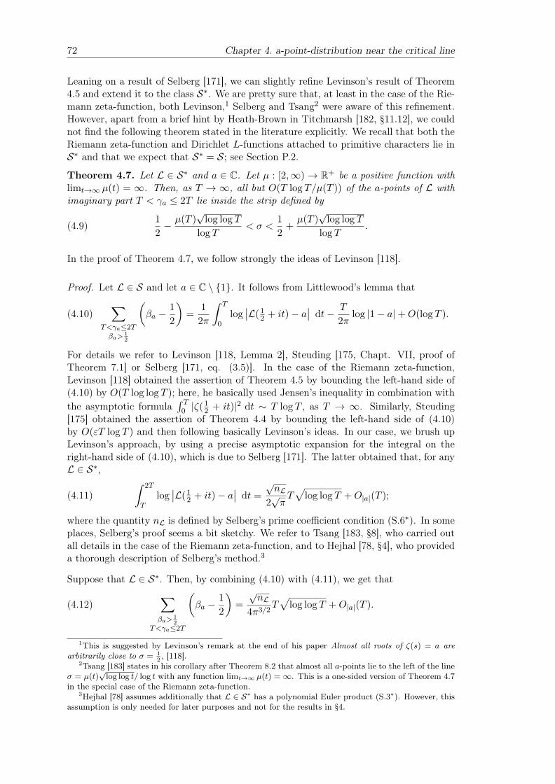
72 Chapter 4. a-point-distribution near the critical line
Leaning on a result of Selberg [171], we can slightly refine Levinson’s result of Theorem4.5 and extend it to the class S∗. We are pretty sure that, at least in the case of the Rie-mann zeta-function, both Levinson,1 Selberg and Tsang2 were aware of this refinement.However, apart from a brief hint by Heath-Brown in Titchmarsh [182, §11.12], we couldnot find the following theorem stated in the literature explicitly. We recall that both theRiemann zeta-function and Dirichlet L-functions attached to primitive characters lie inS∗ and that we expect that S∗ = S; see Section P.2.
Theorem 4.7. Let L ∈ S∗ and a ∈ C. Let µ : [2,∞) → R+ be a positive function withlimt→∞ µ(t) = ∞. Then, as T → ∞, all but O(T log T/µ(T )) of the a-points of L withimaginary part T < γa ≤ 2T lie inside the strip defined by
(4.9)1
2− µ(T )
√log log T
log T< σ <
1
2+µ(T )
√log log T
log T.
In the proof of Theorem 4.7, we follow strongly the ideas of Levinson [118].
Proof. Let L ∈ S and let a ∈ C \ 1. It follows from Littlewood’s lemma that
(4.10)∑
T<γa≤2Tβa>
12
(βa −
1
2
)=
1
2π
∫ T
0log∣∣L(1
2 + it)− a∣∣ dt− T
2πlog |1− a|+O(log T ).
For details we refer to Levinson [118, Lemma 2], Steuding [175, Chapt. VII, proof ofTheorem 7.1] or Selberg [171, eq. (3.5)]. In the case of the Riemann zeta-function,Levinson [118] obtained the assertion of Theorem 4.5 by bounding the left-hand side of(4.10) by O(T log log T ); here, he basically used Jensen’s inequality in combination withthe asymptotic formula
∫ T0 |ζ(1
2 + it)|2 dt ∼ T log T , as T → ∞. Similarly, Steuding[175] obtained the assertion of Theorem 4.4 by bounding the left-hand side of (4.10)by O(εT log T ) and then following basically Levinson’s ideas. In our case, we brush upLevinson’s approach, by using a precise asymptotic expansion for the integral on theright-hand side of (4.10), which is due to Selberg [171]. The latter obtained that, for anyL ∈ S∗,
(4.11)∫ 2T
Tlog∣∣L(1
2 + it)− a∣∣ dt =
√nL
2√πT√
log log T +O|a|(T );
where the quantity nL is defined by Selberg’s prime coefficient condition (S.6∗). In someplaces, Selberg’s proof seems a bit sketchy. We refer to Tsang [183, §8], who carried outall details in the case of the Riemann zeta-function, and to Hejhal [78, §4], who provideda thorough description of Selberg’s method.3
Suppose that L ∈ S∗. Then, by combining (4.10) with (4.11), we get that
(4.12)∑βa>
12
T<γa≤2T
(βa −
1
2
)=
√nL
4π3/2T√
log log T +O|a|(T ).
1This is suggested by Levinson’s remark at the end of his paper Almost all roots of ζ(s) = a arearbitrarily close to σ = 1
2, [118].
2Tsang [183] states in his corollary after Theorem 8.2 that almost all a-points lie to the left of the lineσ = µ(t)
√log log t/ log t with any function limt→∞ µ(t) =∞. This is a one-sided version of Theorem 4.7
in the special case of the Riemann zeta-function.3Hejhal [78] assumes additionally that L ∈ S∗ has a polynomial Euler product (S.3∗). However, this
assumption is only needed for later purposes and not for the results in §4.

Chapter 4. a-point-distribution near the critical line 73
Let µ : [2,∞) → R+ be a positive function with limt→∞ µ(t) = ∞. For positive T , wedenote by N (1)
a (T ) the number of a-points ρa = βa + iγa of L with
βa >1
2+µ(T )
√log log T
log T, T < γa ≤ 2T ;
by N (2)a (T ) the number of a-points with
1
2− µ(T )
√log log T
log T≤ βa ≤
1
2+µ(T )
√log log T
log T, T < γa ≤ 2T ;
and by N (3)a (T ) the number of a-points with
βa <1
2− µ(T )
√log log T
log T, T < γa ≤ 2T.
The trivial estimate ∑βa>
12
T<γa≤2T
(βa −
1
2
)≥ µ(T )
√log log T
log TN (1)a (T )
yields in combination with (4.12) that, for sufficiently large T ,
N (1)a (T ) T log T
µ(T ).
Moreover, for any real b,∑T<γa≤2T
(βa + b) =∑βa>
12
T<γa≤2T
(βa −
1
2
)+
∑βa≤ 1
2T<γa≤2T
(βa −
1
2
)+
∑T<γa≤2T
(1
2+ b
)
≤∑βa>
12
T<γa≤2T
(βa −
1
2
)− µ(T )
√log log T
log TN (3)a (T )+
+
(1
2+ b
)(N (1)a (T ) +N (2)
a (T ) +N (3)a (T )
).
If we take b sufficiently large, we get by means of the asymptotic extensions (4.2) and(4.12) and the Riemann-von Mangoldt formula (4.4) that, for sufficiently large T ,
N (3)a (T ) T log T
µ(T ).
This proves the assertion for a ∈ C \ 1. The case a = 1 can be treated in a similarmanner by relying on suitably adjusted formulas; see the remark at the end of thepreceeding section.
Theorems 4.4, 4.5 and 4.7 hold in an analogous manner for a-points in the lower half-plane.
a-points close to the critical line with real part βa < 12 . Suppose that L ∈ S∗.
Unconditionally, almost nothing is known about how the a-points of Theorem 4.7, which

74 Chapter 4. a-point-distribution near the critical line
lie in the strip (4.9), are distributed to the left and to the right of the critical line. Underthe assumption of the Riemann hypothesis, Selberg [171] obtained the following: forT ≥ 2 and µ > 0, let
σ(T, µ) :=1
2− µ√
log log T
log T.
Then, for every a ∈ C \ 0, as T →∞,
(4.13) Na(σ(T, µ), T ) ∼ Na(T ) · 1√2π
∫ ∞−µ′
e−x2/2 dx
with
µ′ :=
√2dLnL
µ.
Recall that ϕ(x) = 1√2πe−x
2/2 defines the density function of the Gaussian normal dis-tribution. Thus, roughly speaking, Selberg’s result states that about half of the a-pointsof L lie to the left of the critical line and are statistically well distributed at distancesof order
√log log T/ log T . In particular, this means that the left bound of the strip
(4.9) seems to be best possible. Moreover, by assuming the Riemann hypothesis, Selbergdeduced, that, as T → ∞, most of the other a-points with T < γa ≤ 2T in the strip(4.9) lie quite close to the critical line at distances of order not exceeding
O
((log log log T )3
log T√
log log T
).
The proof presented by Selberg [171] is quite sketchy. For a rigorous proof in the specialcase of the Riemann zeta-function, we refer to Tsang [183, Theorem 8.3]. Selberg [171]also provides some heuristic reason in support of the following conjecture.
Selberg’s a-point conjecture. Let L ∈ S. For any a ∈ C \ 0, as T → ∞, about3/4-th of all non-trivial a-points with T < γa ≤ 2T lie to the left of the critical line, andabout 1/4-th of all non-trivial a-points with T < γa ≤ 2T to its right.

Chapter 4. a-point-distribution near the critical line 75
4.3 a-points near the critical line - approach via normalitytheory
In this section we use the concept of filling discs to investigate the a-point distributionof functions L ∈ S# near the critical line. Many of our results hold even for functions inthe more general class G, introduced in Chapter 1.
4.3.1 Filling discs, Julia directions and Julia lines - Definitions andbasic properties
We introduce the notion of filling discs, Julia directions and Julia lines. Roughly speak-ing, these concepts allow a more precise formulation of Picard’s great theorem.
Recall thatM(Ω), resp. H(Ω), denotes the set of all functions which are meromorphic,resp. analytic, on a domain Ω ⊂ C. We say that f ∈M(Ω) satisfies the Picard-propertyon E ⊂ Ω if f assumes on E every value a ∈ C, with at most two exceptions.
Filling discs. We call a sequence of discs Dλn(zn) ⊂ Ω, n ∈ N, a sequence of filling discsfor f ∈M(Ω) if, for arbitrary 0 < ε ≤ 1, the function f satisfies the Picard-property onevery infinite union of the discs Dελn(zn), i.e. on every set of the form
E :=⋃k∈N
Dελnk(znk) with 0 < ε ≤ 1.4
We have necessarily that limn→∞ zn ∈ ∂Ω. Due to rich contributions by French mathe-matical schools,5 filling discs are sometimes referred to as cercles de remplissage.
By Montel’s fundamental normality test (Theorem A.16) and basic convergence proper-ties, the existence of a sequence of filling discs is strongly connected to the non-normalityof a certain family. In fact it is Montel’s fundamental normality test that motivates thedefinition of filling discs and provides a first characterization of the latter.
Proposition 4.8. Let f ∈ M(Ω). Suppose that (zn)n is a sequence of points zn ∈ Ωand (λn)n a sequence of positive real numbers such that Dλn(zn) ⊂ Ω for n ∈ N. Letfn : D→ C be defined by fn(z) := f(zn + λnz).Then, the discs Dλn(zn), n ∈ N, form a sequence of filling discs for f if and only if everyinfinite subset of the family F := fnn is not normal at zero.
The assertion of Proposition 4.8 was observed by many people and, essentially, goes backto Montel [138] and Julia [92].
Proof. Certainly, the functions fn are well-defined on D. Suppose that every infinitesubset of the family F := fnn is not normal at zero. Then, Montel’s fundamentalnormality test (Theorem A.16) implies that every infinite subset of F can omit at mosttwo values a, b ∈ C on any neighbourhood Dε(0) of zero with 0 < ε ≤ 1. By observingthat fn(Dε(0)) = Dελn(zn), this is equivalent to the statement that the discs Dλn(zn),n ∈ N, form a sequence of filling discs for f .
4In the literature it is convenient to demand additionally the growth condition λn ≤ |zn| for the radiiof the filling discs. For our purpose, however, this restriction is not relevant.
5Amongst others, the names of Julia, Milloux and Valiron are here to mention.

76 Chapter 4. a-point-distribution near the critical line
Now, suppose that the discsDλn(zn), n ∈ N, form a sequence of filling discs for f . Assumethat there exists a subsequence (fnk)k of (fn)n which converges locally uniformly on somedisc Dε(0) with 0 < ε ≤ 1. Then, by the theorem of Weierstrass (Theorem A.9), its limitfunction φ is meromorphic on Dε(0). Consequently, taking 0 < ε′ < ε small enough,φ(Dε′(0)) omits a non-empty open subset of C. By uniform convergence, this impliesthat
⋃k≥K fnk(Dε′(0)) omits more than three values for any sufficiently large K ∈ N,
contradicting the definition of filling discs. Consequently, every infinite subset of F isnot normal at zero.
By combining Proposition 4.8 with Marty’s theorem (Theorem A.15), Lehto [114] deriveda powerful characterization of filling discs; we refer here also to Clunie & Hayman [39]and Sauer [163] who pointed out a slight inexactness in Lehto’s original formulation. Forf ∈M(Ω), the spherical derivative f# is defined by
f#(z) :=|f ′(z)|
1 + |f(z)|2 , z ∈ Ω;
for details we refer to the appendix.
Theorem 4.9 (Lehto’s criterion, 1958). Let f ∈M(Ω). Suppose that (zn)n is a sequenceof points zn ∈ Ω and (λn)n a sequence of positive real numbers such that Dλn(zn) ⊂ Ωfor n ∈ N. Then, the discs Dλn(zn), n ∈ N, form a sequence of filling discs for f if andonly if there is a sequence (wn)n of points wn ∈ Ω such that
(4.14) limn→∞
λnf#(wn) =∞ and |zn − wn| = o(λn).
Lehto’s criterion will play a central role in our further investigations.
In a half-strip setting, we equip sequences of filling discs with certain counting functions.Let S be a vertical half-strip in the upper half-plane defined by
(4.15) −∞ < x1 < Re z < x2 < +∞, Im z > 0
For a sequence (zn)n of points zn ∈ S with limn→∞ zn = ∞, we define Nznn(T ) tobe the number of elements in znn with imaginary part less than T . Similarly, forf ∈ M(S), any subset E ⊂ S and any a ∈ C, let Na(E, T ) denote the number ofa-points of f on E with imaginary part less than T .
Lemma 4.10. Let S be a half-strip defined by (4.15) and f ∈ H(S). Let Dλn(zn),n ∈ N, be a sequence of filling discs for f in S such that limn→∞ zn =∞ and Dλn(zn)∩Dλm(zm) = ∅ for n 6= m. Let E :=
⋃n∈NDλn(zn). Then, for all but at most one a ∈ C,
lim supT→∞
Na(E, T )
Nznn(T )> 0.
Proof. Assume that there is an a ∈ C such that
lim supT→∞
Na(E, T )
Nznn(T )= 0.
Then, since the discs Dλn(zn), n ∈ N, are pairwise disjoint, there exists a subsequence(znk)k of (zn)n with
(4.16) limT→∞
Nznkk(T )
Nznn(T )= 1

Chapter 4. a-point-distribution near the critical line 77
such that f omits the values a and ∞ on⋃k∈NDλnk
(znk). Let b ∈ C \ a. Then, wededuce from Proposition 4.8 and an extended version of Montel’s fundamental normalitytest (Theorem A.17 (b)), for any m ∈ N there is an integer K such that f assumes thevalue b more than m-times on every disc Dλnk
(znk) with k ≥ K. Thus, since the discsDλnk
(znk), k ∈ N, are pairwise disjoint, we obtain that for every b ∈ C \ a and everym ∈ N
lim infT→∞
Nb(E, T )
Nznkk(T )> m.
Together with (4.16), this implies that
lim infT→∞
Nb(E, T )
Nznn(T )=∞.
As this holds for any b ∈ C \ a, the assertion is proved.
Julia directions. A complex number eiθ0 with θ0 ∈ R is called Julia direction forf ∈M(Ω) at z0 ∈ ∂Ω if f satisfies the Picard-property in every sectorial domain
ER,ε :=z0 + reiθ ∈ C : 0 < r ≤ R, |θ − θ0| < ε
⊂ Ω
with any ε > 0 and any R > 0. To define a Julia direction for f at z0 = ∞, one has toreplace ER,ε by
E′R,ε :=reiθ ∈ C : r ≥ R, |θ − θ0| < ε
⊂ Ω.
If eiθ0 is a Julia direction for f at z0, then f assumes every value a ∈ C, with at mosttwo exceptions, infinitely often on every set ER,ε, resp. E′R,ε. This follows immediatelyfrom the definition of a Julia direction.
Let f be a function that is analytic in a punctured neighbourhood of an essential singu-larity z0 ∈ C. Lehto [114] proved that
(4.17) lim supz→z0
|z − z0|f#(z) =∞;
here, one has to replace (4.17) by lim supz→z0 |z|f#(z) =∞ if the essential singularity z0
lies at infinity. By means of Lehto’s criterion, we deduce that there is a sequence of pointszn ∈ Ω with limn→∞ zn = z0 such that the discs Dλn(zn), n ∈ N, with λn = |zn − z0|form a sequence of filling discs for f . This implies, in particular, that f satisfies thePicard-property in every punctured neighbourhood of z0. Thus, we have reproducedthe analytic version of Picard’s classical theorem. Moreover, by choosing eiθ0 as anaccumulating point of the set ei arg zn : n ∈ N ⊂ ∂D, we deduce that their exists aJulia direction for f at z0. Thus, we have reproduced the statement of Julia’s classicalresult on Julia directions (see Burckel [29, Theorem 12.27] and Julia [92]).
Julia lines. We call
L := z0 + reiθ0 : r ∈ R with fixed z0 ∈ C, θ0 ∈ [0, 2π)
a Julia line for f ∈M(C) if f satisfies the Picard-property in every open strip containingthe line L.6 Certainly, one can use Lehto’s criterion to detect Julia lines. The followingcorollary is a direct consequence thereof.
6In some literature, the ray reiθ0 , r ∈ R+, connected to a Julia direction eiθ0 is also called Julia line.

78 Chapter 4. a-point-distribution near the critical line
Corollary 4.11. Let f ∈M(C). Suppose that, for a fixed x ∈ R, there exists a sequence(yn)n of positive real numbers yn with limn→∞ yn =∞ and a positive real number α suchthat
limn→∞
|f(x+ iyn)| = α and limn→∞
|f ′(x+ iyn)| =∞.Then, Re z = x defines a Julia line for f .
Proof. For arbitrary λ > 0,
limn→∞
λf#(x0 + iyn) = limn→∞
λ|f ′(x0 + iyn)|
1 + |f(x0 + iyn)|2 =∞.
By Lehto’s criterion (Theorem 4.9), the discs Dλ(x0 + iyn), n ∈ N, form a sequence offilling discs for f and the assertion follows.
Mandelbrojt & Gergen [126] investigated Julia lines of entire functions defined by ageneralized Dirichlet series
A(s) =
∞∑n=0
a(n)e−λns,
which is absolutely convergent in C and satisfies
0 = λ0 < λ1 < λ2 < ... , limn→∞
λn =∞, a(n) 6= 0 for all n > 0.
They derived conditions on the exponents λn and on the growth behaviour of A(s) whichlead to the existence of horizontal Julia lines. Their results mainly rely on the fact thatthe quantities
lim supN→∞
#λn : n ≤ NN
, resp. lim infn→∞
(λn+1 − λn),
are, at least in some mean sense, bounded from above, resp. from below. Thus, theirresults do not apply to ordinary Dirchlet series with non-vanishing coefficients a(n). Forextended results in this direction, we refer to the monographies of Mandelbrojt [127, 128];in [127] particularly to Chapter II for results on analytic functions in strips and ChapterVII for Picard-type results on generalized Dirichlet series in strips, in [128] to Chapter VIagain for Picard-type results. One might interpret the theory developed by Mandelbrojtas a counterpart of lacunary power series for Dirichlet series. It seems that his theory isnot appropriate to describe the value-distribution of functions in the extended Selbergclass.
4.3.2 Julia directions and Julia lines for the Riemann zeta-function
We investigate Julia directions and Julia lines of the Riemann-zeta function. Withsuitable adaptions, similar results can be stated for many functions in the extendedSelberg class. Using another terminology, the following theorem was basically stated byGarunktštis & Steuding [54].
Theorem 4.12. The Julia directions of the Riemann zeta-function are given by eiπ/2,eiπ and ei3π/2.All Julia lines of the Riemann zeta-function are vertical lines. Every line defined byRe z = σ ∈ [1
2 , 1] is a Julia line. There are no Julia lines among the lines Re z = σ ∈(−∞, 0) ∪ (1,∞). Assuming the Riemann hypothesis, the lines Re z = σ ∈ [0, 1
2) are noJulia lines, either.

Chapter 4. a-point-distribution near the critical line 79
Proof. For a given a ∈ C, the discs Dλ(−2n), n ∈ N, with any λ > 0, cover all but finitelymany trivial a-points of the Riemann zeta-function. This follows by a slight refinementof Landau’s proof of Lemma 1 and Lemma 2 in Bohr, Landau & Littlewood [23, Chapt.II]. Thus, they form a sequence of filling discs. Consequently, eiπ is a Julia direction andIm z = 0 defines a Julia line for the zeta-function. As there are left and right half-planesfree of non-trivial a-points, the only further Julia directions are given by eiπ/2 and ei3π/2
and all further Julia lines are vertical lines. Bohr’s and Voronin’s denseness results incombination with Lemma 4.11 yield that every line Re z = σ ∈ (1
2 , 1] is a Julia line. Theclustering of a-points around the critical line (see Theorem 4.7) implies that the same istrue for Re z = 1
2 . By the inequality
ζ(2σ)
ζ(σ)≤ |ζ(s)| ≤ ζ(σ),
which is valid in the half-plane σ > 1, and the functional equation, there is no Juliadirection among Re z ∈ (−∞, 0) ∪ (1,∞). Assuming the Riemann hypothesis, we knowthat, for σ > 1
2 , as t→∞,ζ(σ + it) t−ε
with any ε > 0; see Titchmarsh [182, §14.2]. This in combination with the func-tional equation yields that, under assumption of the the Riemann hypothesis, the linesRe z = σ ∈ [0, 1
2) are no Julia lines either (see Garunkštis & Steuding [54, Lemma 4 andProposition 5]).
In the next section, we shall see that, in main parts, the functional equation is responsiblefor σ = 1
2 being a Julia line.

80 Chapter 4. a-point-distribution near the critical line
4.3.3 Filling discs induced by a Riemann-type functional equation
A Riemann-type functional equation and its symmetry line σ = 12 . A Riemann-
type functional equation for a function G ∈ G invokes a strong connection between Gand G′ on its symmetry line σ = 1
2 .
Lemma 4.13. Let G ∈ G with dG > 0. Then, for t ∈ R with G(12 + it) 6= 0 and
G(12 + it) 6=∞, as |t| → ∞,∣∣∣∣∣G′(1
2 + it)
G(12 + it)
∣∣∣∣∣ ≥ dG2
log |t| − 1
2log(Q2λ) +O
(1
|t|
).
Proof. Logarithmic differentiation of the functional equation yields that
G′(s)
G(s)=
∆′(s)
∆(s)−(G′(1− s)G(1− s)
).
For s = 12 + it, this and the asymptotic extension (1.5) of ∆′/∆ imply that
(4.18) 2 Re
(G′(1
2 + it)
G(12 + it)
)=
∆′(12 + it)
∆(12 + it)
= −dG log |t| − log(Q2λ) +O
(1
|t|
),
provided that |t| is sufficiently large and that s = 12 + it is not a pole of G′(s)/G(s). The
assertion follows from (4.18) by using the relation |z| ≥ |Re z|.
Filling discs induced by a Riemann-type functional equation on σ = 12 . By
Lehto’s criterion, Lemma 4.13 implies that, in most cases, a Riemann-type functionalequation turns σ = 1
2 into a Julia line. The following theorem is a special case of Corollary4.11 for functions satisfying a Riemann-type functional equation.
Theorem 4.14. Let G ∈ G with dG > 0. Suppose that there exists a sequence (τk)k withτk ∈ [2,∞) and limk→∞ τk =∞ and an α ∈ (0,∞) such that
(4.19) limk→∞
|G(12 + iτk)| = α.
Then, for any positive function µ : [2,∞)→ R+ with limτ→∞ µ(τ) =∞, the discs definedby
|s− 12 − iτk| <
µ(τk)
log τk, k ∈ N,
form a sequence of filling discs for G. In particular, σ = 12 is a Julia line of G; and G
assumes every value a ∈ C, with at most two exceptions, infinitely often inside the regiondefined by
(4.20)1
2− µ(t)
log t< σ <
1
2+µ(t)
log t, t ≥ 2.
Proof. Due to our conditions, we can assume without loss of generality that G(12 +iτk) 6=
0,∞ for k ∈ N. We deduce from Lemma 4.13 that∣∣G′(12 + iτk)
∣∣ ≥ dG4
log τk∣∣G(1
2 + iτk)∣∣ ,

Chapter 4. a-point-distribution near the critical line 81
provided that k is large enough. Hence, for sufficiently large k,
G#(12 + iτk) =
|G′(12 + iτk)|
1 + |G(12 + iτk)|2
≥ dG4
log τk|G(1
2 + iτk)|1 + |G(1
2 + iτk)|2
Together with
limk→∞
|G(12 + iτk)|
1 + |G(12 + iτk)|2
=α
1 + α2∈ (0, 1
2 ],
which is true according to our assumption, this yields that
limk→∞
µ(τk)
log τkG#(1
2 + iτk) =∞
for any positive function µ with limτ→∞ µ(τ) =∞. The assertion of the theorem followsimmediately from Theorem 4.9.
For general functionsG ∈ G, the conditions posed onG in Theorem 4.14 are best possible:
Theorem 4.14 does not necessarily apply to functions in G of degree zero: according toKaczorowski & Perelli [94] any function L ∈ S# ⊂ G with dL = 0 is given by a Dirichletpolynomial. Hence, L is bounded in any vertical strip around the critical line.
Condition (4.19) cannot be removed in general as the following two examples show: Letthe function
G000(s) := exp(−s(1− s))∆ζ(s)1/2, s ∈ C∆G000
be defined as in Section 2.3.1. Then, G000 ∈ G with dG000= 1 and limt→∞G000(1
2 + it) = 0.Since
G000(σ + it) exp(−Ct2
)holds uniformly for 0 < σ < 1, as t → ∞, with a certain constant C > 0, the functionG000 ∈ G assumes any given a ∈ C\0 at most finitely often inside the half-strip 0 < σ < 1,t ≥ 2. Thus, the assertion of Theorem 4.14 does not hold for G000. Similarly, the functionG∞∞∞ defined by
G∞∞∞(s) := ∆(s)12 exp(s(1− s)), s ∈ C∆G000
yields an example for a function in G with dG∞∞∞ = 1 and limτ→∞ |G2(12 + iτ)| =∞, but
not satisfying the assertion of Theorem 4.14.
In the general setting of the class G, the radii µ(τk)log τk
of the filling discs are best possible.This can be seen by considering the function
G1,ζ(s) := 1 + ∆ζ(s).
Due to the asymptotic estimate ∆ζ(s) (|t|/2π)1/2−σ, which holds uniformly for 0 ≤σ ≤ 1, as t→∞, the function G1,ζ(s) is bounded in any region defined by
1
2− c
log t≤ σ ≤ 1
2+
c
log t, t > 2,
with an arbitrary constant c > 0.
It seems reasonable to determine the quantities αG,inf and αG,sup defined by (2.12) tocheck whether a given function G ∈ G satisfies condition (4.19). By the intermediate

82 Chapter 4. a-point-distribution near the critical line
value theorem, we find a sequence (τk)k with τk ∈ [2,∞) and limk→∞ τk = ∞ and anα ∈ (0,∞) such that (4.19) holds whenever
αG,inf 6= αG,sup or 0 < αG,inf = αG,sup <∞
For L ∈ S∗ we know that αL,inf = 0 and αL,sup = ∞. We expect that the same is truefor every function L ∈ S#. We refer to Section 3.4.4 for partial results.
Normality approach vs. Levinson’s method. We shall compare the a-point resultof Theorem 4.14, given in terms of filling discs, with the a-point results, obtained byLevinson’s method (Theorems 4.4, 4.5 and 4.7). Both concepts yield qualitatively andquantitatively different information and complement each other: Levinson’s method isappropriate to count the number of a-values in neighbourhoods of line segments 1
2 +it, t ∈[T, 2T ] in a very good manner. Filling discs provide locally more precise information onthe location of some of the a-points (combine for example Theorem A.17 with Proposition4.8). Moreover, the conditions in Theorem 4.14 for the existence of filling discs are ratherweak compared to the conditions needed to evaluate the integrals involved in Levinson’smethod in a precise manner.
In the case of the Riemann zeta-function, Theorem 4.7 provides that almost all non-triviala-values with ordinates 0 < γa ≤ T have a distance less than
µ(γa)√
log log γalog γa
to the critical line; where µ is any positive function tending to infinity. Theorem 4.14yields that, among them, there are infinitely many at distance less than
µ(γa)
log γa
to the critical line.
By assuming certain conjectures, we find filling discs for the Riemann zeta-function whoseradii are significantly smaller than the ones provided by Theorem 4.14. We refer toSection 4.3.5. However, for L ∈ S# the radii of the filling discs cannot shrink arbitrarilyfast, as τ →∞.
Lower bound for the radii of filling discs in S#. The radii λk of a sequence of fillingdiscs Dλk(1
2 + iτk), k ∈ N, for L ∈ S# are trivially bounded from below by |τk|−θL( 12
)−δ,where δ > 0 is an arbitrary positive real number and θL(1
2) defined as in Section 2.3.2.This observation follows from the subsequent lemma.
Lemma 4.15. Let L ∈ S#. Suppose that there are sequences (λk)k, (τk)k with λk, τk ∈R+ and limk→∞ τk =∞ such that Dλk(1
2 + iτk), k ∈ N, forms a sequence of filling discsfor L. Then, for any δ > 0,
limk→∞
(λkτ
θL( 12
)+δ
k
)=∞.
Proof. Assume that there exists a δ > 0 and a subsequence of (λk)k, which we assumeto be (λk)k, such that
λk τ−θL( 1
2)−δ
k

Chapter 4. a-point-distribution near the critical line 83
as k → ∞. We set fk(z) := L(12 + iτk + λkz) and regard the family F := fkk of
functions on D. Then, (2.16) and the continuity of the function θL(σ) assure that
(4.21)∣∣L′(1
2 + iτk + λkz)∣∣δ,` τ
θL(σ)+δ/2k ,
uniformly for z ∈ D, as k →∞. Consequently, we obtain for the spherical derivatives
f#k (z) ≤ λk
∣∣L′(12 + iτk + λkz)
∣∣ τ−θL( 1
2)−δ
k · τ θL(σ)+δ/2k = τ
−δ/2k
uniformly for z ∈ D, as k → ∞. Hence, the family F# := f#k k is bounded on D.
According to Marty’s theorem, F is normal in D. This is in contradiction to Proposition4.8 which states that F is not normal in D.
Generalizations of Theorem 4.14. In Theorem 4.14 we studied filling discs inducedby a Riemann-type functional equation on σ = 1
2 . It would be interesting to investigatewhether similar statements can be retrieved for functions satisfying a different type offunctional equation, for example the Selberg zeta-function.
4.3.4 Filling discs induced by Selberg’s central limit law
In this section, we consider filling discs for functions L ∈ S∗ ⊂ S# which satisfy Selberg’sprime coefficient condition (S.6∗) and the zero-density estimate (DH). Let nL be definedby (S.6∗) and set
gu(t) := exp
(u√
12nL log log t
), t ≥ 2, u ∈ R.
For L ∈ S∗ and α, β ∈ R with α < β, we set
Wgα(t),gβ(t) :=t ∈ [2,∞) : gα(t) ≤
∣∣L(12 + it)
∣∣ ≤ gα(t),
as in Section 3.2.
Theorem 4.16. Let L ∈ S∗ and α, β ∈ R with α < β. Then, for any sequence (τk)kwith τk ∈Wgα(t),gβ(t) ⊂ [2,∞) and limk→∞ τk =∞, the discs defined by
|s− 12 − iτk| <
µ(τk)λα,β(τk)
log τk, k ∈ N,
where µ : [2,∞)→ R+ is any positive function with limt→∞ µ(t) =∞ and
(4.22) λα,β(t) := exp((−α+ max0, 2β)√
12nL log log t),
form a sequence of filling discs for L.
Proof. The existence of a sequence (τk)k with τk ∈Wgα(t),gβ(t) ⊂ [2,∞) and limk→∞ τk =∞ is assured by Theorem 3.1 (a). By Lemma 4.13, we know that, for sufficiently largek ∈ N, ∣∣∣L#(1
2 + iτk)∣∣∣ > 1
3dL log τk|L(1
2 + iτk)|1 + |L(1
2 + iτk)|2.

84 Chapter 4. a-point-distribution near the critical line
Due to the definition of Wgα(t),gβ(t) ⊂ [2,∞), this implies that, for sufficiently largek ∈ N, ∣∣∣L#(1
2 + iτk)∣∣∣ > 1
4dL log τk ·exp(α
√12nL log log τk)
1 + exp(2β√
12nL log log τk)
.
Thus, we obtain that
limk→∞
µ(τk)λα,β(τk)
log τkL#(1
2 + iτk) =∞
for any positive function µ satisfying limt→∞ µ(t) = ∞ and λα,β(t) defined by (4.22).The assertion follows by Lehto’s criterion (Theorem 4.9).
Theorem 3.1 (a) provides a quantitative description of the setWgα(t),gβ(t) ⊂ [2,∞), whichallows us to estimate the number of pairwise disjoint filling discs for L ∈ S∗ in Theorem4.16.
Recall the definition of the counting functions Nznn(T ) and Na(E, T ) introduced inSection 4.3.1. Let L ∈ S∗ and α, β ∈ R with α < β. Further, let λα,β be defined by (4.22)and µ : [2,∞) be a positive function with limt→∞ µ(t) =∞. According to Theorem 3.1and Theorem 4.16, we find a sequence (τk)k of positive real numbers tending to infinitywith
N 12
+iτkk(T ) ≥ N 12
+iτkk(T )−N 12
+iτkk(T2
) T log T
µ(T2
)λα,β(T )
such that the discs defined by
∣∣s− 12 − iτk
∣∣ < µ(τk)λα,β(τk)
log τk, k ∈ N,
form a sequence of pairwise disjoint filling discs for L. By Lemma 4.10, this impliesthat, for every a ∈ C with at most one exception, the number Na(E, T ) of a-points with0 < γa ≤ T inside the region E defined by
12 −
µ(t)λα,β(t)
log t< σ <
1
2+µ(t)λα,β(t)
log t, t ≥ 2.
satisfiesNa(E, T ) T
µ(T2
)λα,β(T )
.
However, by noticing that, for any real α < β and sufficiently large t√log log t < λα,β(t),
we deduce from Theorem 4.7 that Na(E, T ) ∼ dL2πT log T , as T → ∞. Thus, the filling
disc setting of Theorem 4.16 does not beat Theorem 4.7 in counting the a-points insidethe region E.
Nevertheless, as the information retrieved from filling discs is qualitatively different thanthe one provided by Levinson’s method in Theorem 4.7, it is worth stating Theorem4.16.

Chapter 4. a-point-distribution near the critical line 85
4.3.5 Filling discs for the Riemann zeta-function via Ω-results for ζ ′(ρa)
In the case of the Riemann zeta-function there are (conditional) Ω-results for ζ ′(ρa) at ourdisposal which enable us to detect sequences of filling discs whose radii are significantlysmaller than the ones in the general setting of Theorem 4.14.
Discrete moments of ζ ′(s) with respect to non-trivial a-points. Informationabout large values of |ζ ′(ρa)| can be retrieved from asymptotic estimates for discretemoments
Ia(T ) :=1
Na(T )
∑0<γa≤T
ζ ′(ρa), resp. Ja,k(T ) :=1
Na(T )
∑0<γa≤T
∣∣ζ ′(ρa)∣∣2k ;
here Na(T ) denotes as usual the number of non-trivial a-points ρa of the zeta-functionwith imaginary part 0 < γa ≤ T . Asymptotic estimates for Ia(T ) and Ja,k(T ) canbe established by residue methods. Naturally, these asymptotics are powerful tools toestimate the number of simple a-points, in particular the number of simple zeros of theRiemann zeta-function. For works in this direction, we refer to Garunkštis & Steuding[54] concerning simple a-points and exemplarily to Conrey, Gosh & Gonek [42, 43], Bui,Conrey & Young [27] and Bui & Heath-Brown [28] concerning simple zeros.
Garunkštis & Steuding [54] proved that for any fixed a ∈ C, as T →∞,
(4.23) Ia(T ) =1
Na(T )
∑0<γa≤T
ζ ′(ρa) ∼ (12 − a) log
T
2π+ c(a)
with some computable complex constant c(a) depending on a.7 For a = 0, this asymp-totic was already established by Conrey, Gosh & Gonek [42] and later refined by Fujii[52]. From the asymptotic extension (4.23) of Ia(T ), we can immediately deduce thefollowing corollary.
Corollary 4.17. Let a ∈ C \ 12. Then, for every constant 0 < c <
∣∣12 − a
∣∣, there areinfinitely many non-trivial a-points ρa = βa+ iγa of the Riemann zeta-function such that
(4.24)∣∣ζ ′(ρa)∣∣ ≥ c log |γa|.
Proof. Let a ∈ C \ 12 and 0 < c <
∣∣12 − a
∣∣. Assume that for all but finitely manynon-trivial a-points ρa, we have ∣∣ζ ′(ρa)∣∣ < c log |γa|.
Then, as T →∞,
(4.25) |Ia(T )| ≤ 1
Na(T )
∑0<γa≤T
∣∣ζ ′(ρa)∣∣ < c log T + o(1).
This is, however, in contradiction to (4.23).
By Lehto’s criterion (Theorem 4.9), we are now able to show the following.7Actually, Garunkštis & Steuding [54] obtained even a more precise asymptotic formula. They also
give a heuristic explanation why the leading term log T vanishes in the case a = 12.

86 Chapter 4. a-point-distribution near the critical line
Theorem 4.18. For a ∈ C \ 12, there exists a sequence (ρa,k)k of non-trivial a-points
of the Riemann zeta-function with ordinates γa,k > 0 such that the discs defined by
|s− ρa,k| <µ(γa,k)
log γa,k, k ∈ N,
with any positive function µ : [2,∞)→ R+ satisfying limt→∞ µ(t) =∞, form a sequenceof filling discs for ζ.
Proof of Theorem 4.18. Let (ρa,k)k be a sequence of non-trivial a-points with positiveimaginary parts such that (4.24) holds. Then, for any positive function with limt→∞ µ(t),we have
limk→∞
µ(γa,k)
log γa,kζ#(ρa,k) = lim
k→∞
µ(γa,k)
log γa,k
|ζ ′(ρa,k)|1 + |a|2 =∞.
The theorem follows by Lehto’s criterion (Theorem 4.9).
As far as the author knows, non-trivial conditional or unconditional asymptotic estimatesfor Ja,k(T ) are only known in the case a = 0.
Discrete moments of ζ ′(s) with respect to non-trivial zeros. Gonek [58] andHeijhal [77] conjectured independently that J0,k(T ) (log T )k
2+2k for k ∈ R, as T →∞.Hughes, Keating & O’Connell [82] conjectured that J0,k(T ) ∼ Ck(log T )k
2+2k for k >−3/2, as T →∞, with an explicit computable constant Ck derived from models for theRiemann zeta-function by random matrix theory. Assuming the Riemann hypothesis,Gonek [57] obtained that J0,1 ∼ 1
12(log T )3 and Ng [145] that J0,2 (log T )8. Usinga method developed by Rudnick & Soundararajan [162] and assuming the generalizedRiemann hypothesis (GRH) for Dirichlet L-functions, Milinovich & Ng [133] could derivelower bounds for the discrete moments J0,k(T ). For k ∈ N, as T →∞,
(4.26) J0,k(T ) =1
N(T )
∑0<γ≤T
∣∣ζ ′(ρ)∣∣2k (log T )k
2+2k.
where N(T ) := N0(T ) denotes, as usual, the number of non-trivial zeros of ζ withimaginary part 0 < γ ≤ T . The assumption of the GRH is required to derive a suitableasymptotic formula for sums of the shape∑
0<γ≤Tζ ′(ρ)AX(ρ)k−1AX(1− ρ)k
with AX(s) =∑
n≤X n−s. Originally, Milinovich [132] deduced this asymptotic formula
from the main theorem of Ng [146] where it was enough to assume the Riemann hy-pothesis. Later, they discovered a serious mistake in the error term of the asymptoticexpansion in the main theorem of Ng [146]. However, as they indicate in [133], it appearsthat this mistake may be fixed with additional effort. Under the assumption of the Rie-mann hypothesis, Milinovich [134] could bound J0,k(T ) from above by (log T )k
2+2k+ε
with an arbitrary ε > 0. This upper bound together with the lower bound (4.26) sup-ports the conjecture by Gonek [58], Heijhal [77] and Hughes, Keating & O’Connell [82].The following corollary is an immediate consequence of Milinovich’s & Ng’s lower bound(4.26).

Chapter 4. a-point-distribution near the critical line 87
Corollary 4.19. Assume the GRH for Dirichlet L-functions. For δ > 0, let A be theset of all non-trivial zeros ρ of the Riemann zeta function satisfying∣∣ζ ′(ρ)
∣∣ ≥ (log |γ|)δ.
Then, for any η > 0, as T →∞, NA(T ) T 1−η. 8
Proof. For a given δ > 0, we choose K ∈ N such that K2 + 2K > 2Kδ. We denote by Athe set of all non-trivial zeros ρ of the Riemann zeta function satisfying |ζ ′(ρ)| ≥ (log |γ|)δ.Analogously, we denote by B the set of all non-trivial zeros ρ for which |ζ ′(ρ)| < (log |γ|)δis true. Assume that there exists a real number η > 0 such that NA(T ) T 1−η, asT →∞. Then, it follows from the Riemann-von Mangoldt formula that NB(T ) ∼ N(T ),as T → ∞. Under the assumption of the Riemann hypothesis, we know that all non-trivial zeros are on the line σ = 1
2 and that ζ(12 + it) tε for any ε > 0, as t → ∞.
Taking ε = η/2K and putting everything together, we obtain that, as T →∞,
J0,K(T ) =1
N(T )
∑0<γ≤T
∣∣ζ ′(ρ)∣∣2K
1
N(T )
(NA(T ) · T 2K· η
2K +NB(T ) · (log T )2Kδ)
(log T )2Kδ.
By our choice of K, this is in contradiction to (4.26). The assertion is proved.
By Lehto’s criterion (Theorem 4.9), we are now able to show the following.
Theorem 4.20. Assume the GRH for Dirichlet L-functions. Then, for every δ > 0,there is a set A of non-trivial zeros ρ = 1
2 + iγ of the Riemann zeta-function withNA(T ) T 1−η for any η > 0, as T →∞, such that the discs defined by
|s− ρ| < 1
(log |γ|)δ , ρ ∈ A,
form a sequence of filling discs for ζ(s).
Proof. For a given δ > 0, we define A to be the set of all non-trivial zeros ρ = 12 + iγ of
the Riemann zeta-function satisfying
|ζ ′(12 + iγ)| ≥ (log |γ|)δ+1.
Then, Corollary 4.19 assures that NA(T ) T 1−η for any η > 0, as T →∞. Moreover,
lim|γ|→∞
12
+iγ∈A
1
(log |γ|)δ ζ#(1
2 + iγ) = lim|γ|→∞
12
+iγ∈A
1
(log |γ|)δ∣∣ζ ′(1
2 + iγ)∣∣ =∞.
and the theorem follows by Lehto’s criterion (Theorem 4.9).8The function NA(T ) counts all elements in A with positive imaginary part less or equal to T . For a
precise definition, we refer to Section 4.3.1.

88 Chapter 4. a-point-distribution near the critical line
Soundararajan’s resonance method. A resonance method developed by Sounda-rarajan [172] yields another approach to retrieve information about large values of ζ ′(ρ).Ng [147] showed that, under assumption of the GRH for Dirichlet L-functions, there areinfinitely many non-trivial zeros such that
ζ ′(ρ) exp
(c0
log |γ|log log |γ|
)where c0 = 1√
2− ε with any ε > 0. By Lehto’s criterion, we deduce the following.
Theorem 4.21. Assume the GRH for Dirichlet L-functions. Then, there exists a se-quence (ρk)k of non-trivial zeros ρk = 1
2 + iγk of the Riemann zeta-function with γk > 0such that the discs defined by
|s− ρk| < µ(γk) exp
(−c0
log γklog log γk
), k ∈ N,
form a sequence of filling discs for ζ(s), where µ : [2,∞)→ R+ is any positive functionsatisfying limt→∞ µ(t) =∞.
Proof. According to Ng [147], for any fixed 0 < c0 <√
2, there exist a constant C > 0and a sequence (ρk)k of non-trivial zeros ρk = 1
2 + iγk of the Riemann zeta-function withγk > 0 such that ∣∣ζ ′(ρk)∣∣ ≥ C exp
(c0
log γklog log γk
)for every k ∈ N. Hence, for any positive function µ satisfying limt→∞ µ(t) =∞,
limk→∞
µ(γk) exp
(−c0
log |γk|log log |γk|
)ζ#(ρk)
= limk→∞
µ(γk) exp
(−c0
log |γk|log log |γk|
)|ζ ′(ρk)|
=∞.
The assertion follows by Lehto’s criterion (Theorem 4.9).
4.4 Non-trivial a-points to the left of the critical line
According to Selberg’s a-point conjecture, we expect that, for any a ∈ C\0, about 3/4-th of the non-trivial a-points of the Riemann zeta-function lie to the left of the criticalline. However, unconditionally, it is not even known whether there are infinitely manynon-trivial a-points to the left of the critical line. This motivated Steuding to raise thefollowing question at the problem session of the 2011 Palanga conference in honour ofJonas Kubilius. Is it possible to find for every a ∈ C a sequence of points sk = σk + itk,k ∈ N, with σk < 1
2 and limk→∞ tk =∞ such that
limk→∞
ζ(sk) = a.
By means of our results in Section 3.3 concerning small and large values in a neighbour-hood of the critical line, we can give a very first answer to this question.

Chapter 4. a-point-distribution near the critical line 89
Corollary 4.22. Let c > 0 and let ε : [2,∞)→ R be a function satisfying
0 < ε(t) ≤ c
log tfor t ≥ 2.
Then, for every α > 0, there exists an a ∈ C with |a| = α and a sequence (tk) withtk ∈ [1,∞) such that
limk→∞
ζ(12 − ε(tk) + itk) = a.
Proof. The case α = 0 follows directly from Corollary 3.3. Thus, suppose that α > 0. Ifwe take m = α+1 in Corollary 3.3, the intermediate value theorem assures the existenceof a sequence (tk)k with tk ∈ [1,∞) and limk→∞ tk =∞ such that
ζ(12 − ε(tk) + itk) ∈ ∂Dα(0)
for all k ∈ N. As the circle ∂Dα(0) is compact, the set ζ(12 − ε(tk) + itk)k∈N ⊂ ∂Dα(0)
has at least one accumulation point a ∈ ∂Dα(0). Thus, there is a subsequence (tkj )j of(tk)k such that
limj→∞
ζ(12 − ε(tkj ) + itkj ) = a.
4.5 Summary: a-points of the Riemann zeta-function nearthe critical line
Let λ be a positive function on R with limt→∞ λ(t) = 0 and Sλ be the region defined by
12 − λ(t) < σ < 1
2 + λ(t), t ≥ 2.
In the following corollary, we summarize our knowledge on how fast λ(t) can tend tozero, as t→∞, such that, for a given a ∈ C, there are almost all, a positive proportion,resp. infinitely many of all non-trivial a-points of the Riemann zeta-function inside Sλ.For more detailed information the reader is referred to the corresponding theorems ofthe preceeding sections.
Corollary 4.23 (Levinson, Selberg, Tsang, Christ).
(a) Unconditionally, for every a ∈ C, there are almost all a-points of the Riemannzeta-function (in the sense of density) inside the region Sλ if one chooses
λ(t) =µ(t)√
log log t
log t, t ≥ 2,
with any positive function µ satisfying limt→∞ µ(t) =∞.9
9This follows from Theorem 4.7 which was proved in the framework of the class S∗ by refining amethod developed by Levinson [118] with results of Selberg [171], Tsang [183] and Steuding [175].
90 Chapter 4. a-point-distribution near the critical line
(b) Under the assumption of the Riemann hypothesis, for every a ∈ C, there is apositive proportion of all a-points of the Riemann zeta-function (in the sense ofdensity) inside the region Sλ if one chooses
λ(t) =c√
log log t
log t, t ≥ 2,
with any constant c > 0.10
(c) Unconditionally, for every a ∈ C, with at most one exception, there are infinitelymany a-points of the Riemann zeta-function inside the region Sλ if one chooses
λ(t) =µ(t)
log t, t ≥ 2,
with any positive function µ satisfying limt→∞ µ(t) =∞.11
Moreover, one knows unconditionally that almost all zeros of the Riemann zeta-function (in the sense of density) lie in this region.12
(d) Under the assumption of the Riemann hypothesis, for every a ∈ C, there are in-finitely many a-points of the Riemann zeta-function inside the region Sλ if onechooses
λ(t) =µ(t)(log log log t)3
log t√
log log t, t ≥ 2,
with any positive function µ satisfying limt→∞ µ(t) =∞.13
(e) Under the assumption of the GRH for Dirichlet L-functions,14 for every a ∈ C,with at most one exception, there are infinitely many a-points of the Riemann zeta-function inside the region Sλ if one chooses
λ(t) =1
(log t)δ, t ≥ 2,
with any δ > 0.15
(f) Under the assumption of the GRH for Dirichlet L-functions, for every a ∈ C, withat most one exception, there are infinitely many a-points of the Riemann zeta-function inside the region Sλ if one chooses
λ(t) = µ(t) exp
(−c0
log t
log log t
), t ≥ 2
with any positive function µ satisfying limt→∞ µ(t) = ∞ and any constant 0 <c0 <
1√2.16
10This is due to Selberg [171]; see Section 4.1.11This follows from Theorem 4.14 which was proved in the framework of the class G by relying on
normality arguments.12This is due to Selberg [168]; see Theorem 4.6.13This is due to Selberg [171]; see Section 4.1.14Very likely this can be also obtained by only assuming RH; see the remarks in Section 4.3.5.15This follows from Theorem 4.20which was deduced by certain normality arguments from a result of
Milinovich & Ng [133].16This follows from Theorem 4.21 which was deduced by certain normality arguments from a result
of Ng [147].

Chapter 5
Denseness results for the Riemannzeta-function in the critical strip
The critical line is a natural boundary for the universality property of the Riemannzeta-function. Even if we slightly change the concept, the functional equation stronglyrestricts the set of approximable functions; see Chapter 2.
In this chapter we investigate a concept of universality for the Riemann zeta-function onthe critical line that is significantly weaker than the one regarded in Chapter 2. Roughlyspeaking, we set the scaling factor of the limiting process introduced in Section 2.2 tobe constantly equal to zero and drop our request to approximate analytic functions,but restrict to the approximation of complex points a ∈ C by shifts of the Riemannzeta-function on the critical line.
We know that, for every α ∈ [0,∞), there exist a sequence (τk)k of real numbers τk ∈[2,∞) with limk→∞ τk =∞ such that
limk→∞
∣∣ζ(12 + iτk)
∣∣ = α;
see Section 3.4.4. However, except for a = 0, we do not know explicitly any other exampleof an accumulation point a ∈ C of the set
V (12) := ζ(1
2 + it) : t ∈ [1,∞).
According to a conjecture of Ramachandra, we expect that
V (12) = C,
i.e., we conjecture that the values of the Riemann zeta-function on the critical lie densein C. However, to prove or disprove this conjecture with present day’s methods seemsto be out of reach.
Bohr [15, 16, 21, 22] and his collaborators established denseness results for the zeta-valueson vertical lines inside the strip 1
2 < σ ≤ 1. It were their pioneering works that directedVoronin towards his universality theorem. In Section 5.1, we state the main results ofBohr and his collaborators on the value-distribution of the Riemann zeta-function tothe right of the critical line. We briefly report on their methods and discuss why thesemethods fail to obtain a denseness statement for the zeta-values on the critical line.
91

92 Chapter 5. Denseness results for the Riemann zeta-function in the critical strip
In Section 5.2, we point out that a denseness result for the critical line is qualitativelydifferent from the one on vertical lines in 1
2 < σ ≤ 1.
We know that 0 ∈ V (12). According to Ramachandra’s conjecture, we expect that 0 is in
particular an interior point of V (12). In Section 5.3, we show that there is a subinterval
A ⊂ [0, 2π) of length at least π4 such that, for every θ ∈ A, there is a sequence (tn)n of
numbers tn ∈ [2,∞) with
ζ(12 + itn) 6= 0, lim
n→∞ζ(1
2 + itn) = 0 and arg ζ(12 + itn) ≡ θ mod 2π.
In Section 5.4, we approach Ramachandra’s conjecture by asking whether there are curves[1,∞) 3 t 7→ 1
2 + ε(t) + it with limt→∞ ε(t) = 0 such that the values of the Riemannzeta-function on these curves lie dense in C. We obtain some positive answers both byrelying on the a-point results of Section 4.3 and by relying on Bohr’s work.
In Section 5.5, we see that the latter question is much easier to handle if we regard curveswhich do not approach the left but the right boundary line of the strip of universality,i.e. the line σ = 1.
Finally, in Section 5.6, we briefly indicate what happens to the limiting process of Section2.2 if we adjust the underlying conformal mappings such that they map D to discs whichlie completely inside the strip 1
2 < σ < 1, but arbitrarily close to the critical line.
Although we mainly restrict to the Riemann zeta-function in this chapter, most of theresults are true for related functions from quite general classes.
5.1 The works of Bohr and Voronin
At the beginning of the 20th century, Bohr and his collaborators studied the value-distribution of the Riemann zeta-function to the right of the critical line.
Value-distribution on vertical lines in σ > 1. Due to the pole of the Riemannzeta-function at s = 1, the characteristic convergence abscissae of the Dirichlet seriesexpansion of the Riemann zeta-function are given by σc = σu = σa = 1. Thus, accordingto Bohr [17], the behaviour of the zeta-function on vertical lines in the half-plane σ > 1is ruled by almost periodicity; see Theorem 3.7. For every fixed σ > 1, we know that
ζ(2σ)
ζ(σ)≤ |ζ(σ + it)| ≤ ζ(σ) for t ∈ R.
and that these inequalities are sharp; see Apostol [2, Chapt. 7.6]. As
limσ→∞
ζ(2σ)
ζ(σ)= lim
σ→∞ζ(σ) = 1, lim
σ→1+
ζ(2σ)
ζ(σ)= 0 and lim
σ→1+ζ(σ) =∞,
the setV (σ) := ζ(σ + it) : t ∈ [1,∞)
contracts to 1, as σ →∞, and contains both arbitrarily small and arbitrarily large values,as σ → 1. Beyond this observation, we know that, for every σ > 1, the set
log ζ(σ + it) : t ∈ R

Chapter 5. Denseness results for the Riemann zeta-function in the critical strip 93
lies dense in an area of C which is either simply connected and bounded by a convexcurve or which is ring-shaped and bounded by two convex curves; see Bohr & Jessen[21] or Titchmarsh [182, §11.6]. Essential ingredients in the proof are the Euler productrepresentation of the Riemann zeta-function and diophantine approximation.
Bohr’s denseness results on vertical lines in 12 < σ ≤ 1. Bohr & Courant [15]
proved that the values taken by the Riemann zeta-function on an arbitrary vertical lineinside the strip 1
2 < σ ≤ 1 form a dense set in C, i.e.
V (σ) = C for every σ ∈ (12 , 1].
In fact, their proof yields the stronger statement that, for every σ ∈ (12 , 1], every a ∈ C
and every ε > 0,
(5.1) lim infT→∞
1
Tmeas t ∈ [1,∞) : |ζ(σ + it)− a| < ε > 0.
Even more precise results were obtained by Bohr & Jessen [22] and Laurinčikas [111,Chapt. 4], who established probabilistic limit theorems for the values of the logarithmof the zeta-function on vertical lines. In particular, Laurinčikas [111, Chapt. 4, Theorem4.1] showed that, for every σ > 1
2 , there exists a Borel probability measure µσ such that,for every continuous and bounded function f : C→ C,
limT→∞
1
2T
∫ T
−Tf(log ζ(σ + it)
)dt =
∫Cf(z) dµ(z).
If σ ∈ (12 , 1] the support of µσ is the whole complex plane.
Voronin’s denseness results on vertical lines in 12 < σ ≤ 1. Voronin [186] estab-
lished multidimensional extensions of Bohr’s denseness result. For any n ∈ N0 and anyfunction f ∈ H(Ω), we define
∆nf(s) :=(f(s), f ′(s), ..., f (n)(s)
)to be the (n+1)-dimensional vector consisting of the values of f and its first n derivativesevaluated at the point s ∈ Ω. Among other things, Voronin [186] obtained that
(5.2) ∆nζ(σ + it) : t ∈ [1,∞) = Cn+1 for every σ ∈ (12 , 1]
and every n ∈ N0. By a slight refinement of Voronin’s proof, one obtains that, for everyσ ∈ (1
2 , 1], every a ∈ Cn+1 and every ε > 0
(5.3) lim infT→∞
1
Tmeas t ∈ (0, T ] : ‖∆nζ(σ + it)− a‖ < ε > 0;
here and in the following ‖ · ‖ denotes the maximum-norm in the complex vector spaceCn+1. It was this multidimensional extension of Bohr’s result that inspired Voronin [187]to prove his universality theorem (Theorem P.1). In fact, for 1
2 < σ < 1, the densenessresults (5.3) and (5.1) are direct consequences of Voronin’s universality theorem.
Bohr’s method. To prove his denseness result, Bohr modeled the Riemann zeta-function by truncated Euler products
ζN (σ + it) =∏p≤N
(1− p−σ−it
)−1;

94 Chapter 5. Denseness results for the Riemann zeta-function in the critical strip
here the product is taken over all prime numbers p ∈ P with p ≤ N . We fix 12 < σ ≤
1. Bohr noticed that the quantities p−it = e−it log p with p ∈ P, p ≤ N , behave likeindependent random variables, although they all depend on the common variable t.1
Relying on the theory of convex curves and diophantine approximation, in particulara theorem of Kronecker and Weyl, he was able to prove that, for given a ∈ C, thereexists a large subset A ⊂ [1,∞) such that, for all t ∈ A, the truncated Euler productζN (σ + it) is quite close to a. Although ζN (σ + it) does not converge in 1
2 < σ ≤ 1, asN →∞, Bohr showed that the truncated Euler product approximates the zeta-functionin mean-square. Here, the essential tool is the existence of the mean-square value
limT→∞
∫ T
1|ζ(σ + it)|2 dt <∞
for 12 < σ ≤ 1 in combination with Carlson’s theorem. From the approximation in
mean-square, Bohr deduced that there exists a large subset B ⊂ [1,∞) such that, forall t ∈ B, the truncated Euler product ζN (σ + it) is close to ζ(σ + it). Finally, certaindensity estimates assure that A ∩ B 6= ∅ and the result follows. Voronin obtained hisdenseness statement (5.2) basically by refining the ideas of Bohr.
Non-denseness results on vertical lines in σ < 12 . On vertical lines in the half-plane
σ < 12 , we expect that the zeta-function grows too fast than that its values could lie dense
in C. It follows essentially from the functional equation that
(5.4) V (σ) 6= C for σ ≤ 0;
see Garunkštis & Steuding [54]. By assuming the Riemann hypothesis, Garunkštis &Steuding [54] proved that (5.4) persists for all σ < 1
2 . Their proof uses a conditionalΩ-result for the zeta-function on vertical lines in σ > 1
2 together with the functionalequation.
We know that V (σ) = C for 12 < σ ≤ 1 and we expect that V (σ) 6= C for 0 < σ < 1
2 .But how is the situation if σ = 1
2?
Is V (12) = C? During the 1979 Durham conference, Ramachandra formulated the con-
jecture that the values of the Riemann zeta-function on the critical line lie dense in C.Until now, this could not be proved or disproved. The difficulty in handling the valuesof the zeta-function on the critical line is that, due to Hardy & Littlewood [71],
1
T
∫ T
−T
∣∣ζ(12 + it)
∣∣2 dt ∼ log T,
as T →∞. Hence, Bohr’s method collapses on the critical line.
Jacod, Kowalski & Nikeghbali [90] introduced a new type of convergence in probabil-ity theory, which they called ‘mod-Gaussian convergence’. For a given sequence (Zn)nof real-valued random variables Zn, this concept builds basically on working with thecorresponding sequence of characteristic functions (E[eiuZn ])n. Leaning on this type ofconvergence, Kowalski & Nikeghbali [108] were able to show that
V (12) = C
would follow rather directly from a suitable version of the Keating-Snaith moment con-jectures. By generalizing the notion of ‘mod-Gaussian convergence’, Delbaen, Kowalski& Nikeghbali [47] obtained the following quantitative result.
1see Bohr & Jessen [21, p. 6].

Chapter 5. Denseness results for the Riemann zeta-function in the critical strip 95
Theorem 5.1 (Delbaen, Kowalski & Nikeghbali, 2011). If for any k > 0 there exist areal number Ck ≥ 0 such that
(5.5)∣∣∣∣ 1
T
∫ T
0exp
(it · log ζ(1
2 + iu))du∣∣∣∣ ≤ Ck
1 + |t|4(log log T )2
holds for T ≥ 1 and t ∈ R with |t| ≤ k, then, for any bounded Jordan measurable subsetB ⊂ C,
limT→∞
12 log log T
Tmeas
t ∈ (0, T ] : log ζ(1
2 + it) ∈ B
= 12πmeas B.
Models for the zeta-function based on links to random matrix theory suggest that (5.5)should hold; see Keating & Snaith [104, 105].
5.2 Qualitative difference of the value-distribution on thecritical line
A possible denseness statement for the values of the Riemann zeta-function on the criticalline is qualitatively different from the one on vertical lines in 1
2 < σ ≤ 1.
Garunkštis & Steuding [54] showed that, due to the functional equation, a multidimen-sional denseness result in the sense of (5.2) does not hold on the critical line. We caneasily generalize their result to the class G.
Theorem 5.2. Let G ∈ G. Then,(G(1
2 + it), G′(12 + it)) : t ∈ [1,∞)
6= C2.
Proof. We follow the ideas of Garunkštis & Steuding [54]. The basic ingredient in theproof is the observation that for real t of sufficiently large modulus with G(1
2 + it) 6= 0and G(1
2 + it) 6=∞,
(5.6)
∣∣∣∣∣G′(12 + it)
G(12 + it)
∣∣∣∣∣ ≥ dG2
log |t| − 1
2log(Q2λ) +O
(1
|t|
);
see Lemma 4.13. We fix (a, b) ∈ C2 with a, b 6= 0 and set, for a given 0 < ε < min|a|, |b|,
Dε(a, b) :=
(s1, s2) ∈ C2 : |s1 − a| < ε and |s2 − b| < ε
Assume thatW :=
(G(1
2 + it), G′(12 + it)) : t ∈ [1,∞)
= C2.
Then, in particular, Dε(a, b) ⊂W . Due to (5.6), we can fix t0 > 1 such that∣∣∣∣∣G′(12 + it)
G(12 + it)
∣∣∣∣∣ > |b|+ ε
|a| − ε
for all t ≥ t0 with G(12 + it) 6= 0 and G(1
2 + it) 6=∞. By the choice of t0, it follows that(G(1
2 + it), G′(12 + it)) : t ∈ [t0,∞)
⊂ C \Dε(a, b).

96 Chapter 5. Denseness results for the Riemann zeta-function in the critical strip
-2 -1 1 2 3 4 5Re z
-4
-2
2
4Im z
(a) V ( 32
)
-2 -1 1 2 3 4 5Re z
-4
-2
2
4Im z
(b) V (1)
-2 -1 1 2 3 4 5Re z
-4
-2
2
4Im z
(c) V ( 78
)
-2 -1 1 2 3 4 5Re z
-4
-2
2
4Im z
(d) V ( 34
)
-2 -1 1 2 3 4 5Re z
-4
-2
2
4Im z
(e) V ( 58
)
-2 -1 1 2 3 4 5Re z
-4
-2
2
4Im z
(f) V ( 12
)
-2 -1 1 2 3 4 5Re z
-4
-2
2
4Im z
(g) V ( 38
)
-2 -1 1 2 3 4 5Re z
-4
-2
2
4Im z
(h) V ( 14
)
-2 -1 1 2 3 4 5Re z
-4
-2
2
4Im z
(i) V ( 18
)
Figure 5.1: For some σ ∈ R, we plotted the set V50(σ) := ζ(σ + it) : t ∈ [0, 50]restricted to the range −2 ≤ Rez ≤ 6, −4 ≤ Imz ≤ 4.
Consequently, we have
Dε(a, b) ⊂
(G(12 + it), G′(1
2 + it)) : t ∈ [1, t0]
=: W ∗.
This, however, yields a contradiction.
Moreover, according to Selberg’s central limit law, the curve t 7→ ζ(12 +it) has a preference
to visit arbitrarily small neighbourhoods of zero than the ones of any other complex value.
Theorem 5.3. Let a ∈ C and 0 < ε < |a|. Then,
limT→∞
1
Tmeas
t ∈ (0, T ] :
∣∣ζ(12 + it)− a
∣∣ < ε
=
0 if a 6= 0,12 if a = 0.

Chapter 5. Denseness results for the Riemann zeta-function in the critical strip 97
Comparing this with (5.1), we see once more that the value-distribution on the criticalline is qualitatively different.
Proof. According to Theorem 3.1 (b), Selberg’s central limit law implies that, for arbi-trary ε > 0, as T →∞,
1
Tmeas
t ∈ (0, T ] : |ζ(1
2 + it)| < ε
= 12 + o(1).
This proves the case a = 0. Moreover, according to Theorem 3.1 (b), Selberg’s centrallimit law yields that, for arbitrary a ∈ C, a 6= 0 and any 0 < ε∗ < |a|,
1
Tmeas
t ∈ (0, T ] : |a| − ε∗ < |ζ(1
2 + it)| ≤ |a|+ ε∗,= o(1),
as T →∞. Due to the observation that, for any 0 < ε < ε∗ and any T > 0,
0 ≤ 1
Tmeas
t ∈ (0, T ] : |ζ(1
2 + it)− a| < ε
≤ 1
Tmeas
t ∈ (0, T ] : |a| − ε∗ < |ζ(1
2 + it)| ≤ |a|+ ε∗,
the statement for a 6= 0 follows.
5.3 Approaching zero and infinity from different directions
Although the curve t 7→ ζ(12 + it) has a preference to be either close to zero or to infinity,
it is neither known whether zero is an interior point of the set
V (12) =
ζ(1
2 + it) : t ∈ [1,∞)⊂ C
nor whether zero is an interior point of the setζ(1
2 + it)−1 : t ∈ [1,∞)⊂ C.
Relying on Theorem 3.2, resp. Corollary 3.3, we prove that we can approximate zeroand infinity with non-zero values in V (1
2) from quite many directions.
Theorem 5.4. Let L ∈ S∗. Then, there exist real numbers θ0, θ∞ ∈ [0, 2π) with thefollowing properties.
(a) For every θ ∈ (θ0 − π8 , θ0 + π
8 ), there exist a sequence (tk)k with tk ⊂ (1,∞] andlimk→∞ tk =∞ such that
L(12 + itk) ∈ eiθR+ :=
reiθ : r ∈ R+
for k ∈ N and
limk→∞
L(12 + itk) = 0.
(b) For every θ ∈ (θ∞ − π8 , θ∞ + π
8 ), there exist a sequence (tk)k with tk ⊂ (1,∞] andlimk→∞ tk =∞ such that
L(12 + itk) ∈ eiθR+
for k ∈ N andlimk→∞
L(12 + itk) =∞.

98 Chapter 5. Denseness results for the Riemann zeta-function in the critical strip
Proof. We only prove statement (a). Statement (b) can be proved by essentially thesame method.
For L ∈ S∗, there is an analogue of Hardy’s Z-function at our disposal which allows usto write for sufficiently large real t, say t ≥ t0,
L(12 + it) = ZL(t)∆L(1
2 + it)1/2.
For the definition and basic properties of ZL(t) the reader is referred to Section 1.2.Recall here, in particular, that for t ≥ t0,
ZL(t) ∈ R and ∆L(12 + it)1/2 ∈ ∂D.
We fix an arbitrary 0 < q < 12 and set κL := π
2dL. Then, according to Theorem 3.2 (b),
resp. Corollary 3.3 (b), we find a sequence (τk)k with τk ∈ [t0,∞) and limk→∞ τk = ∞such that the functions
Lτk(y) := L(
12 + i
κLlog τk
y + iτk
)= ZL
(κL
log τky + τk
)∆L
(12 + i
κLlog τk
y + iτk
)1/2
do not vanish on the interval [−q, q] for k ∈ N and converge uniformly on [−q, q] to zero,as k →∞.
As the functions Lτk(y), k ∈ N, are real and non-vanishing on the interval [−q, q], wefind, for every k ∈ N, an integer ηk ∈ −1,+1 such that
fk(y) := ηk · ZL(
κLlog τk
y + τk
)> 0 for y ∈ [−q, q] .
The factors ηk assure that fk(y) = |Lτk(y)| for k ∈ N and y ∈ [−q, q]. Further, weobserve that, uniformly for y ∈ [−q, q],(5.7) fk(y)→ 0, as k →∞.Now, we set
hk(y) := η−1k ·∆L
(12 + i
κLlog τk
y + iτk
)1/2
.
Observe that |hk(y)| = 1 and that
(5.8) fk(y) · hk(y) = Lτk(y)
for k ∈ N and y ∈ [−q, q]. Since hk(0) ∈ ∂D, it follows from the compactness of ∂Dthat the set hk(0)k has at least one accumulation point eiθ0 ∈ ∂D with θ0 ∈ [0, 2π).Without loss of generality, we may suppose that
limk→∞
hk(0) = eiθ0 .
Otherwise, we work with a suitable subsequence of (hk(0))k. For k ∈ N, we defineθk ∈ [0, 2π) such that eiθk = hk(0). Then, according to Lemma 2.3, we have, uniformlyfor y ∈ [−q, q],
hk(y) = hk(0) · exp(−i1
2dLκLy)(
1 +O
(1
log τk
))= exp
(iθk − iπ4 y
)(1 +O
(1
log τk
)).

Chapter 5. Denseness results for the Riemann zeta-function in the critical strip 99
as k → ∞. Thus, for any θ ∈ (θ0 − qπ4 , θ0 + qπ
4 ), we find for sufficiently large k ∈ N, areal number yk ∈ [−q, q] with(5.9) hk(yk) = exp(iθ).
Now, we settk := τk +
κLlog τk
yk.
Then, according to (5.7), (5.8) and (5.9), we have L(12 + itk) ∈ eiθR+ for all sufficiently
large k ∈ N and limk→∞ L(12 + itk) = 0. As we can choose arbitrary 0 < q < 1
2 , theassertion is proved.
For the Riemann zeta-function, there are results of Kalpokas, Korolev & Steuding [102] atour disposal which exceed the statement of Theorem 5.4 (b) by far. Kalpokas & Steuding[101] investigated intersection points of the curve R 3 t 7→ ζ(1
2 + it) with straight lineseiθR := reiθ : r ∈ R through the origin. In particular, they observed that
ζ(12 + it) ∈ eiθR ⇐⇒ ζ(1
2 + it) = 0 or ∆ζ(12 + it) = ei2φ.
Their works were extended by Christ & Kalpokas [36, 37] and Kalpokas, Korolev &Steuding [102]. The latter showed that, for every θ ∈ [0, 2π), there is a sequence (tk)kwith tk ∈ R and limk→∞ tk =∞ such that, for all k ∈ N,
ζ(12 + itk) ∈ eiθR+ and |ζ(1
2 + itk)| ≥ C(log tk)5/4
with some positive constant C. Thus, roughly speaking, the values of the Riemannzeta-function on the critical line expand in every direction.
Korolev showed in a talk at the ELAZ conference 2012 at Schloss Schney that thereexists a sequence (tk)k with tk ∈ R and limk→∞ tk =∞ such that, for every k ∈ N,
ζ(12 + itk) ∈ R \ 0 and lim
k→∞ζ(1
2 + itk) = 0.
Korolev’s result is not published yet.
5.4 Denseness results on curves approaching the critical line
In the following, let ε : [1,∞)→ R be a function with limt→∞ ε(t) = 0. For a humble at-tack on Ramachandra’s conjecture, we investigate the value-distribution of the Riemannzeta-function on curves t 7→ 1
2 + ε(t) + it which approach the critical line asymptoticallyas t→∞.
If we could establish a denseness statement for the zeta-values on curves approachingthe critical line sufficiently fast, then the denseness of the zeta-values on the critical linewould follow; see the subsequent theorem. Recall the definition of the function θL(σ)from Section 2.3.2, which indicates the order of growth of a given function L ∈ S#.
Theorem 5.5. Let L ∈ S# and n ∈ N0. Let ε : [1,∞) → R be a function such thatε(t) t−θL( 1
2)−δ, as t→∞, with some δ > 0. Then,
∆nL(12 + it) : t ∈ [1,∞)
= Cn+1
if and only if ∆nL(1
2 + ε(t) + it) : t ∈ [1,∞)
= Cn+1.

100 Chapter 5. Denseness results for the Riemann zeta-function in the critical strip
Proof. Let a ∈ Cn+1 and ε > 0. Let ‖ · ‖ denote the maximum-norm in the complexvector space Cn+1. Then, according to Lemma 2.6, there exist a constant t0 > 1 suchthat ∥∥∆nL(1
2 + ε(t) + it)−∆nL(12 + it)
∥∥ < ε/2
for t ≥ t0. Assume that
∆nL(12 + ε(t) + it) : t ∈ [1,∞)
= Cn+1. Then, we find a
t∗ ≥ t0 such that ∥∥∆nL(12 + ε(t∗) + it∗)− a
∥∥ < ε/2.
By means of the triangle inequality, we obtain that∥∥∆nL(12 + it∗)− a
∥∥< ε.
As we can choose a ∈ Cn+1 and ε > 0 arbitrarily in the argumentation above, we deducethat
∆nL(12 + it) : t ∈ [1,∞)
= Cn+1.
The other implication of the theorem can be proved by the same argument.
A negative denseness results on curves approaching the critical. The propertyof the Riemann zeta-function that a multidimensional denseness result does not hold onthe critical line carries over to certain curves approaching the critical line.
Corollary 5.6. Let L ∈ S# and n ∈ N. Let ε : [1,∞) → R be a function such thatε(t) t−θL( 1
2)−δ, as t→∞, with some δ > 0. Then,
∆nL(12 + ε(t) + it) : t ∈ [1,∞)
6= Cn+1.
Proof. Recalling that S# ⊂ G and noticing that n 6= 0, the corollary follows directly bycombining Theorem 5.2 with Theorem 5.5.
Denseness results on curves approaching the critical line. It seems difficult toobtain a denseness result on curves t 7→ 1
2 + ε(t) + it by adapting Bohr’s method. Thisis due to the fact that, according to a result of Laurinčikas [112], there is a quantitativeswap in the asymptotic behaviour of the mean-square near the critical line.
Theorem 5.7 (Laurinčikas, 1991). Let µ : [2,∞)→ R be a non-negative, (not necessarilystrictly) monotonically increasing or decreasing function satisfying limT→∞
µ(T )log T = 0.
(a) If limT→∞ µ(T ) =∞, then, as T →∞,
1
T
∫ T
2
∣∣∣∣ζ (12 +
µ(T )
log T+ it
)∣∣∣∣2 dt ∼ 1
2µ(T )log T.
(b) If limT→∞ µ(T ) = c with some c > 0, then, as T →∞,
1
T
∫ T
2
∣∣∣∣ζ (12 +
µ(T )
log T+ it
)∣∣∣∣2 dt ∼ 1
2c
(1− e−2c
)log T.
(c) If limT→∞ µ(T ) = 0, then, as T →∞,
1
T
∫ T
2
∣∣∣∣ζ (12 +
µ(T )
log T+ it
)∣∣∣∣2 dt ∼ log T.

Chapter 5. Denseness results for the Riemann zeta-function in the critical strip 101
12 + µ(τ)
log τ + iτ
b
b
b
b
b
b
b
s2
s3
s4
s5
12 − µ(τ)
log τ + iτ
12 + ǫ(τ) + iτ
Re(s)
Im(s)
0 12
2
Figure 5.2: The construction of the curve t 7→ 12 + ε(t) + it in the proof of Theorem
5.8.
For a proof we refer to Laurinčikas [112, Theorems 1, 2 and 3].
Nevertheless, we can use the a-point results from Chapter 4 to deduce the existence ofcertain curves on which the values of the zeta-function lie dense in C.
Theorem 5.8. There exists a continuous function ε : [2,∞) → R with limt→∞ ε(t) = 0such that
ζ(12 + ε(t) + it) : t ∈ [2,∞)
= C.
Here we can demand additionally that,
(a) unconditionally,
|ε(t)| ≤ µ(t)
log t
with any positive function µ satisfying limt→∞ µ(t) =∞.
(b) by assuming the Riemann hypothesis,
|ε(t)| ≤ µ(t)(log log log t)3
log t√
log log t
with any positive function µ satisfying limt→∞ µ(t) =∞.
(c) by assuming the generalized Riemann hypothesis for Dirichlet L-functions,2
|ε(t)| ≤ 1
(log t)δ
with any δ > 0.2Very likely this can be proved by only assuming the Riemann hypothesis; see the remarks in Section
4.3.5.

102 Chapter 5. Denseness results for the Riemann zeta-function in the critical strip
(d) by assuming the generalized Riemann hypothesis for Dirichlet L-functions,
|ε(t)| ≤ µ(t) exp
(−c0
log t
log log t
)with any positive function µ satisfying limt→∞ µ(t) = ∞ and any constant 0 <c0 <
1√2.
Proof. Let (qk)k be an enumeration of Q + iQ. According to Corollary 4.23 (c), we findfor every qk, with at most one exception, infinitely many roots of the equation ζ(s) = qkinside the strip S defined by
12 −
µ(t)
log t< σ < 1
2 +µ(t)
log t, t ≥ 2,
where µ is an arbitrarily positive function satisfying limt→∞ µ(t). Without loss of gener-ality, we may suppose that the enumeration (qk)k is arranged such that q1 is the possiblyexisting value which is not assumed by the zeta-function in S. This agreement as well asthe observation above assure that we find points sk = σk + itk ∈ S such that ζ(sk) = qkand tk < tk+1 for every k ∈ N \ 1. By connecting the point sk with its successor sk+1,respectively, by a straight line segment, we get a continuous function ε : [2,∞) → R+
such that |ε(t)| ≤ µ(t)log t for all t ∈ [2,∞) and 1
2 + ε(tk) + itk = sk for all k ∈ N. Theorem5.8 (a) follows then immediately as Q+ iQ (minus the possibly existent exceptional valueq1) is dense in C.
The statements (b), (c) and (d) follow from Corollary 4.23 (d), (e) and (f) in an analogousmanner.
The curves of Theorem 5.8 can oscillate from the left to the right of the critical line. Itwould be nice to have a similar statement for curves which stay always either to the leftor to the right of the critical line.
Curves approaching the critical line from the left. From Selberg’s conditionalresult concerning a-points to the left of the critical line, we deduce the following densenessstatement.
Theorem 5.9. Assume that the Riemann hypothesis is true. Then, for arbitrary 0 <c1 < c2, there exists a continuous function ε : [1,∞)→ R with
c1√
log log t
log log t≤ ε(t) ≤ c2
√log log t
log log t
such that ζ(1
2 − ε(t) + it) : t ∈ [1,∞)
= C.
Proof. Relying on Selberg’s result (4.13), the proof follows along the lines of the proofof Theorem 5.8.
Curves approaching the critical line from the right. Relying on Bohr’s, resp.Voronin’s denseness result, it is possible to prove the following theorem.

Chapter 5. Denseness results for the Riemann zeta-function in the critical strip 103
Theorem 5.10 (Christ [35], 2012). For every n ∈ N0, there is a positive, piecewise-constant function ε : [1,∞)→ R+ with limt→∞ ε(t) = 0 such that
∆nζ(
12 + ε(t) + it
): t ∈ [1,∞)
= Cn+1.
Proof. To prove Theorem 5.10 we use Voronin’s denseness result in combination witha certain enumeration method. Let (εk)k and (σk)k be sequences with εk > 0 andσk ∈ (0, 1
2) for k ∈ N that tend to zero as k →∞. Furthermore, for a given n ∈ N0, wedefine compact sets
Ak := z ∈ Cn+1 : ‖z‖ ≤ k, k ∈ N.
The sets Ak form a countable covering of the (n+ 1)-dimensional complex plane, i.e.⋃k∈N
Ak = Cn+1.
We set T0 = 1 and choose, inductively for k ∈ N, a positive real number Tk > Tk−1 + 1such that for all a ∈ Ak there is a τ ∈ (Tk−1, Tk] with∥∥∆nζ
(12 + σk + iτ
)− a∥∥ < εk.
The existence of such a number Tk is assured by Voronin’s denseness result applied tothe vertical line σ = 1
2 +σk and basic properties of compact sets. The piecewise-constantfunction ε : [1,∞)→ R+ defined by
ε(t) = σk for t ∈ (Tk−1, Tk] with k ∈ N,
satisfies limt→∞ ε(t) = 0. The construction of the function ε yields that the curve t 7→12 + ε(t) + it has the desired property.
As we are very flexible in choosing the zero-sequences (εk)k, (σk)k and a proper countablecovering of the complex plane (Ak)k∈N, the proof of Theorem 5.10 yields the existenceof uncountable many curves with the desired property.
By adjusting the sets Ak in a proper way, we can use a quantitative version of Voronin’sdenseness result (see Karatsuba & Voronin [103, Chapt. VIII]) to get very rough esti-mates on how ‘fast’ these curves approach the critical line.
With respect to Theorem 5.6, it would be very nice to characterize the changeover of∆2ζ(1
2 + ε(t) + it) : t ∈ [1,∞) from denseness to non-denseness in terms of the speedof convergence of ε(t)→ 0, as t→∞.
Small and large values on curves approaching the critical line. From Corollary3.3, which we obtained by relying on Selberg’s central limit law, we can deduce informa-tion on small and large values of the zeta-function on certain curves t 7→ 1
2 + ε(t) + it.
Corollary 5.11. Let c > 0 and ε : [1,∞) → R be a function satisfying |ε(t)| ≤ clog t for
t ∈ [1,∞). Then,
lim inft→∞
|ζ(12 + ε(t) + it)| = 0 and lim sup
t→∞|ζ(1
2 + ε(t) + it)| =∞.

104 Chapter 5. Denseness results for the Riemann zeta-function in the critical strip
(a) |ζ(σ + it)| (b) |ζ(σ + it)|−1
Figure 5.3: The values |ζ(σ + it)| and |ζ(σ + it)|−1 on the rectangular region 0.3 ≤σ ≤ 0.7 and 1000 ≤ t ≤ 1005.
Proof. The corollary follows directly from Corollary 3.3 by working with the conformalmap ϕτ (z) = 1
2 +κζ/4log τ z + iτ and the rectangular domain R( 4c
κζ, 1).
Roughly speaking, Corollary 5.11 states that the zeta-function assumes both arbitrarilysmall and arbitrarily large values on every path to infinity which lies inside the strip
12 −
c
log t< σ < 1
2 +c
log t, t ≥ 1,
with arbitrary c > 0.
5.5 Denseness results on curves approaching the line σ = 1
By a slight refinement of Bohr’s method, we can show that the values of the zeta-functiontaken on any curve [1,∞) 3 t 7→ 1 + ε(t) + it with limt→∞ ε(t) = 0 are dense in C.
Theorem 5.12 (Christ [35], 2012). Let ε : [1,∞)→ R be a function with limt→∞ ε(t) =0. Then, for every a ∈ C and ε > 0,
lim infT→∞
1
Tmeas t ∈ (0, T ] : |ζ(1 + ε(t) + it)− a| < ε > 0.
We choose the function ε in Theorem 5.12 such that the curve t 7→ 1 + ε(t) + it liescompletely in the half-plane σ > 1. In this case, Theorem 5.12 cannot be deduced fromVoronin’s universality theorem. Moreover, in Theorem 5.12, there are no restrictions onhow fast ε(t) tends to zero as t→∞.
Proof. To prove Theorem 5.12, we rely on the methods of Bohr & Courant [15] andBohr & Jessen [22] who proved a corresponding result for vertical lines inside the strip12 < σ ≤ 1. We will refine their methods by adding a certain continuity argument. AsBohr and his collaborators did, we will prove the result not for ζ(s), but for log ζ(s).The result for ζ(s) is then an immediate consequence therefrom. We define log ζ(s) forσ > 1
2 in a standard way; for details we refer to Steuding [175, Chapt. 1.2]

Chapter 5. Denseness results for the Riemann zeta-function in the critical strip 105
Let ε > 0 and a ∈ C. Let (pn)n be an enumeration of all prime numbers in ascendingorder. For a positive integer N , we define the truncated Euler product
ζN (s) =
N∏n=1
(1− p−sn )−1.
Note that ζN (s) defines an analytic and non-vanishing function in the half-plane σ > 0.Bohr showed that there is positive real number d and a positive integer N1 such that,for all N ≥ N1, we find a subset I(N) ⊂ (0,∞) of lower density
lim infT→∞
1
Tmeas (I(N) ∩ (0, T ]) > d
with the property that
| log ζN (1 + it)− a| < ε/3 for t ∈ I(N).
Furthermore, Bohr proved that, for any ε′ > 0 and any 12 < σ0 < 1, there is a positive
real numbers N2 such that, for every N ≥ N2 and every σ ≥ σ0,
limT→∞
1
T
∫ T
1
∣∣∣∣ ζ(σ + it)
ζN (σ + it)− 1
∣∣∣∣ dt < ε′.
The bounded convergence theorem assures that
limT→∞
∫ T
1
∫ 2
σ0
∣∣∣∣ ζ(σ + it)
ζN (σ + it)− 1
∣∣∣∣2 dσ dt < 2ε′
By carefully adopting Bohr’s reasoning, we can deduce from the estimate above that thereexists a positive integer N3 such that, for all N ≥ N3, we find a subset J (N) ⊂ (0,∞)of lower density
lim infT→∞
1
Tmeas (J (N) ∩ (0, T ]) > 1− d
with the property that
| log ζN (1 + ε(t) + it)− log ζ(1 + ε(t) + it)| < ε/3 for t ∈ J (N).
Now, we apply a certain continuity argument. We fix N0 ≥ maxN1, N3 and choose asufficiently small δ < log(1 − ε
6N0)−1/(N0 log 2). As limt→∞ ε(t) = 0, we find a positive
number T0 such that ε(t) < δ for t ≥ T0. Then, for t ≥ T0,
|log ζN0(1 + it)− log ζN0(1 + ε(t) + it)| =∣∣∣∣∣N0∑n=1
log
(1 +
1− p−ε(t)n
p1+itn − 1
)∣∣∣∣∣≤
N0∑n=1
2
∣∣∣∣∣1− p−ε(t)n
p1+itn − 1
∣∣∣∣∣ ≤ 2N0(1− p−ε(t)N0) < 2N0(1− 2−N0δ) < ε/3.
Here, we used Betrand’s postulate which states that pn ≤ 2n. Although the estimationvia Bertrand’s postulate is quite rough, it is completely sufficient for our purpose.
Altogether, we can deduce that the setM := I(N0)∩J (N0)∩(T0,∞) has positive lowerdensity, i.e.
lim infT→∞
1
Tmeas (M∩ (0, T ]) > 0,

106 Chapter 5. Denseness results for the Riemann zeta-function in the critical strip
and enjoys the property that
| log ζ(1 + ε(t) + it)− a| ≤ | log ζ(1 + ε(t) + it)− log ζN0(1 + ε(t) + it)|+ | log ζN0(1 + ε(t) + it)− log ζN0(1 + it)|+ | log ζN0(1 + it)− a| < ε
for t ∈M. The statement of the theorem follows.
5.6 A limiting process to the right of the critical line
In this final section of Part I, we briefly discuss what happens to the limiting process ofSection 2.2 if we adjust the underlying conformal mappings such that they map the unitdisc to discs which lie completely inside the strip 1
2 < σ < 1, but arbitrarily close to thecritical line. By relying on Voronin’s universality, we can prove the following statement.
Theorem 5.13. Let 0 ≤ η ≤ 14 and let (εk)k, (λk)k be sequences with εk, λk ∈ R,
0 < λk < εk <14 for k ∈ N and limk→∞ εk = limk→∞ λk = η. Further, let
ζk,τ (z) := ζ(12 + εk + λkz + iτ) for τ ≥ 1, k ∈ N and z ∈ D.
Then, there is a sequence (τk)k with τk ∈ [1,∞) and limk→∞ τk = ∞ such that, forevery continuous and non-vanishing function g on D which is analytic in D, there is asubsequence of (ζk,τk)k which converges uniformly on D to g.
Sketch of the proof. Due to the theorem of Mergelyan, see for example [161], it is suffi-cient to establish the assertion of Theorem 5.13 for polynomial target functions g whichhave rational coefficients and do not vanish on D. The proof follows then directly fromVoronin’s universality theorem in combination with a similar enumeration method asthe one that we used in the proof of Theorem 5.10. We refer to Christ [35] for moredetails.

Part II
Discrete and continuous moments
107


109
In part II we aim at extending a result of to Tanaka [179] who established a weak versionof the Lindelöf hypothesis for the Riemann zeta-function.
Recall that, according to Hardy & Littlewood [69], the Lindelöf hypothesis is equivalentto the statement that, for every σ > 1
2 and k ∈ N,
(5.10) limT→∞
1
T
∫ T
1|ζ(σ + it)|2k dt =
∞∑n=1
dk(n)2
n2σ,
where dk denotes the generalized divisor function appearing in the Dirichlet series ex-pansion of ζk. Tanaka showed that (5.10) holds if one neglects a certain set A ⊂ [1,∞)of density zero from the path of integration.
In the sequel, let 111X denote the indicator function of a set X ⊂ R and Xc := R \ Xits complement. So far, formula (5.10) is proved only in the cases k = 1, 2, due toclassical works of Hardy & Littlewood [68] and Ingham [86]. This is sufficient to derivethe following boundedness property of the Riemann zeta-function in σ > 1
2 : for everyε > 0 and α > 1
2 , there exist a constant Mε > 0 and a subset B ⊂ [1,∞) of upper density
lim supT→∞
1
T
∫ T
1111B(t) dt < ε
such that
(5.11) |ζ(σ + it)| ≤Mε for σ ≥ α and t ∈ Bc.
This follows from a standard method which we shall explain later on in the proof ofLemma 8.2 (b).
In particular, we deduce from (5.11) that, for every ε > 0 and α > 12 , there exist a
constant Mε > 0 and a subset B ⊂ [1,∞) of upper density
lim supT→∞
1
T
∫ T
1111B(t) dt < ε
such that, for every σ ≥ α and k ∈ N,
(5.12) lim supT→∞
1
T
∫ T
1|ζ(σ + it)|2k 111Bc(t) dt ≤M2k
ε .
This provides already a weak version of Tanaka’s result.

110
Tanaka used some additional ergodic theoretical reasoning to control the limit in (5.12)as ε→ 0. He obtained that, for every ε > 0 and α > 1
2 , there exist a subset A ⊂ [1,∞)of density
limT→∞
1
T
∫ T
1111A(t) dt = 0
such that, for every σ ≥ α and k ∈ N,
limT→∞
1
T
∫ T
1|ζ(σ + it)|2k 111Ac(t) dt =
∞∑n=1
dk(n)2
n2σ.
We extend Tanaka’s result to a large class of functions which we shall denote by N . Werely here essentially on the ideas and methods developed by Tanaka [179].
Two features of a function L are crucial in order to obtain an asymptotic expansion forthe second power moment (k = 1) of L in the sense of Tanaka:
(i) In the half-plane σ > 1, the function L is represented by a Dirichlet series
L(s) =∞∑n=1
a(n)
ns, σ > 1,
with coefficients a(n) ∈ C satisfying
∞∑n=1
|a(n)|2nσ
<∞, for σ > 1.
(ii) The function L satisfies a certain normality feature in the half-plane σ > 12 which we
shall define later on in Section 8.1. This normality feature is more or less equivalentto the boundedness property (5.11) stated above for the Riemann zeta-function.
In order to obtain asymptotic expansions for the 2k-th moment for L in the sense ofTanaka with k ∈ N, it is necessary that both L and its k-th powers Lk satisfy property(i). For this purpose, we study in Chapter 6 the Dirichlet series expansions of Lk andother functions related to a given Dirichlet series L. Here, we mainly work with Dirichletseries that satisfy the Ramanujan hypothesis.
Dirichlet series can be modeled by an ergodic flow on the infinite dimensional torus. Weoutline this concept in Chapter 7 and focus especially on the results which we shall needlater on to prove our extended version of Tanaka’s result in Chapter 9.
In Chapter 8 we define the normality feature stated in property (ii) above and set upthe class N . We investigate basic properties of functions in N which we shall need lateron to prove our main result.
In Chapter 9 we state and prove our main theorem, i.e. an extended version of Tanaka’sresult.

Chapter 6
Arithmetic functions and Dirichletseries coefficients
In this chapter we study the Dirichlet series expansions of certain functions related toa given Dirichlet series L. We start with some basic properties of certain arithmeticfunctions.
6.1 Arithmetic functions connected to the Riemann zeta-function
A function a : N→ C is said to be an arithmetic function. According to the fundamentaltheorem of arithmetic, for every n ∈ N and every prime number p ∈ P with p|n, thereexist uniquely determined quantities ν(n; p) ∈ N such that
(6.1) n =∏p∈Pp|n
pν(n;p).
We call an arithmetic function a : N→ C multiplicative if
a(n) =∏p∈Pp|n
a(pν(n;p)) for n ∈ N.
If a satisfies the stronger property
a(n) =∏p∈Pp|n
a(p)ν(n;p) for n ∈ N,
we call the function a completely multiplicative. For two arithmetic functions a, b : N→C, the arithmetic function a ∗ b : N→ C defined by
(a ∗ b)(n) :=∑
(n1,n2)∈N2
n1n2=n
a(n1)b(n2) for n ∈ N
is said to be the Dirichlet convolution of a and b.
111

112 Chapter 6. Arithmetic functions and Dirichlet series coefficients
We associate a given arithmetic function a : N→ C, n 7→ a(n) with the formal Dirichletseries
L(s) =
∞∑n=1
a(n)
ns,
and vice versa. We say that the coefficients of a given Dirichlet series are (completely)multiplicative if its associated arithmetic function is (completely) multiplicative. If theDirichlet series
L1(s) =
∞∑n=1
a(n)
nsand L2(s) =
∞∑n=1
b(n)
ns
converge absolutely for a given s ∈ C, then their product L1(s)·L2(s) is also an absolutelyconvergent Dirichlet series given by
(6.2) L1(s) · L2(s) =
∞∑n=1
(a ∗ b)(n)
ns.
The generalized divisor function. We fix κ ∈ R and define, for every prime numberp ∈ P and every ν ∈ N0,
dκ(pν) :=
(κ+ ν − 1
ν
),
where the generalized binomial coefficient is defined in a standard way:(x
0
):= 1 and
(x
ν
):=
1
ν!
ν−1∏j=0
(x− j) for x ∈ R and ν ∈ N.
From the functional equation of the Gamma-function, we derive that
dκ(pν) =Γ(κ+ ν)
Γ(κ)ν!.
We setdκ(n) :=
∏p∈Pp|n
dκ(pν(n;p)).
for every n ∈ N and refer to the arithmetic function dκ : N → N defined by n 7→ dκ(n)as generalized divisor function with parameter κ. By definition, the function dκ is mul-tiplicative. The Dirichlet series associated with dκ can be identified with the Dirichletseries expansion of ζ(s)κ := exp(κ log ζ(s)) in σ > 1, where log ζ(s) is defined in a stan-dard way. For details we refer to Tenenbaum [180, Chapt. II.5.1] or Heath-Brown [72].In the following lemma, we gather some well-known properties of the generalized divisorfunction if its allied parameter is an integer. In this case, dκ has an important numbertheoretical interpretation: for k ∈ N, the quantity dk(n) counts the representations ofn ∈ N as a product of k natural numbers; additionally, we have d−k(n) = 0 if and onlyif there exist a prime number p with p|n such that ν(n; p) ≥ k + 1.
Lemma 6.1. Let k ∈ N.
(a) For n ∈ N,
d0(n) =
1 if n = 1,
0 if n 6= 1,and d1(n) = 1.

Chapter 6. Arithmetic functions and Dirichlet series coefficients 113
(b) The function dk is the k-fold Dirichlet convolution of d1. In particular, for n ∈ N,
dk(n) =∑
(n1,...,nk)∈Nkn1···nk=n
1.
(c) For sufficiently large n ∈ N,
1 ≤ dk(n) ≤ exp
((k − 1) log 2
log n
log log n
(1 +O
(log log log n
log logn
))).
(d) The function d−1 is the classical Möbius function µ. In particular, for n ∈ N,
d−1(n) = µ(n) =
(−1)r if n = p1 · · · pr with pairwise distinct p1, ..., pr ∈ P,0 otherwise.
(e) The function d−k is the k-fold Dirichlet convolution of d−1. In particular, for p ∈ Pand ν ∈ N with ν ≥ k + 1,
d−k(pν) = 0.
(f) For n ∈ N, we have |d−k(n)| ≤ dk(n).
Sketch of the proof: The statements (a) and (d) follow directly from the definition of dkand a short computation. As the Dirichlet series associated with dk can be identified asthe Dirichlet series expansion of ζ(s)k in σ > 1, we obtain that
ζ(s)k =
( ∞∑n=1
1
ns
)k=
∞∑n=1
dk(n)
ns, σ > 1.
Therefrom, we deduce that
(6.3) dk = dk−1 ∗ d1 = d1 ∗ ... ∗ d1︸ ︷︷ ︸k-times
.
Hence, dk is the k-fold Dirichlet convolution of d1. This implies that
(6.4) dk(n) =∑
(n1,...,nk)∈Nkn1···nk=n
1 for n ∈ N.
Alternatively, the latter identity can be derived from the fundamental theorem of arith-metics and a combinatorial argument. Altogether, statement (b) follows. By standardestimates, we obtain that, for sufficiently large n ∈ N,
(6.5) d2(n) ≤ exp
(log 2
log n
log logn
(1 +O
(log log log n
log log n
)));
see, for example, Steuding [175, Chapt. 2.3] or Hardy & Wright [70, Chapt. 18.1]. Itfollows from (6.3) that, for n ∈ N,
dk(n) =∑
(n1,n2)∈N2
n1·n2=n
dk−1(n1)d1(n2) ≤ dk−1(n) ·∑
(n1,n2)∈N2
n1·n2=n
1 = dk−1(n) · d2(n).

114 Chapter 6. Arithmetic functions and Dirichlet series coefficients
Iteratively, we obtain that
dk(n) ≤ d2(n)k−1 for n ∈ N.
Together with (6.5), this proves the upper bound for dk(n) in statement (c). The lowerbound for dk(n), i.e.
dk(n) ≥ 1 for n ∈ N,
follows immediately from the definition of dk. The identity
ζ(s)−k =
( ∞∑n=1
d−1(n)
ns
)k=
∞∑n=1
d−k(n)
ns, σ > 1.
implies that d−k is the k-fold Dirichlet convolution of d−1. Moreover, we deduce fromthe definition of dκ that, for any κ ∈ R, p ∈ P and ν ∈ N,
(6.6) dκ(pν) =1
ν!
ν−1∏j=0
(κ− ν + 1− j) =1
ν!
ν−1∏j=0
(κ+ j).
If we set κ = −k in (6.6), then zero occurs as a factor in the products on the righthand-side, whenever ν ≥ k + 1. Statement (e) follows. Moreover, we deduce from (6.6) that,for p ∈ P and ν ∈ N,
|d−k(pν)| =
∣∣∣∣∣∣ 1
ν!
ν−1∏j=0
(−k + j)
∣∣∣∣∣∣ ≤ 1
ν!
ν−1∏j=0
(k + j) = dk(pν).
Statement (f) follows then from the multiplicity of d−k and dk.
Now, we state some basic properties of dκ in the general situation if its allied parameterκ is an arbitrary real number.
Lemma 6.2. Let κ ∈ R. Then, the following statements are true.
(a) If κ ≥ 0, then dκ(n) ≥ 0 for n ∈ N. If κ ≥ 1, then dκ(n) ≥ 1 for n ∈ N.
(b) For n ∈ N and K ≥ |κ|, we have |dκ(n)| ≤ dK(n).
(c) There is an absolute constant c > 0 such that, for every p ∈ P and every ν ∈ N0,
dκ(pν) < c|κ|νκ−1.
(d) For sufficiently large n ∈ N,
|dκ(n)| ≤ exp
(c(κ) log 2
log n
log logn
(1 +O
(log log log n
log logn
))).
where c(κ) := minn ∈ N : n ≥ |κ| − 1.
(e) For m ∈ N, the function dmκ is the m-fold Dirichlet convolution of dκ. In particu-lar, for n ∈ N,
dmκ(n) =∑
(n1,...,nm)∈Nmn1···nm=n
dκ(n1) · · · dκ(n2) =∏p∈Pp|n
∑k1,...,km∈N0
k1+...+km=ν(n;p)
m∏j=1
dκ(pkj ).

Chapter 6. Arithmetic functions and Dirichlet series coefficients 115
Proof. Let κ ∈ R. It follows immediately from (6.6) and the multiplicativity of dκ that,for n ∈ N,
dκ(n) ≥
0 if κ ≥ 0,
1 if κ ≥ 1.
Statement (a) is proved. Similarly, we derive statement (b) from the observation that,for p ∈ P, ν ∈ N and any K ≥ |κ|,
|dκ(pν)| ≤ 1
ν!
ν−1∏j=0
(|κ|+ j) ≤ dK(pν).
Now, we rewrite (6.6) in the form
(6.7) dκ(pν) =κ
ν·ν−1∏j=1
(1 +
κ
j
).
By using the inequality 1 + x ≤ exp(x), which is true for any real x, we obtain that, forp ∈ P and ν ∈ N,
|dκ(pν)| ≤ |κ|ν
exp
κ ν−1∑j=1
1
j
.
A standard asymptotic estimate for the partial sums of the harmonic series yields theexistence of an absolute constant c > 0 such that, for every p ∈ P and every ν ∈ N0,
dκ(pν) < c|κ|νκ−1.
Statement (c) is proved. Statement (d) follows by combining the estimates of statement(b) and Lemma 6.1 (c). The identity
∞∑n=1
dκm(n)
ns= ζ(s)κm = (ζ(s)κ)m =
( ∞∑n=1
dκ(n)
ns
)mimplies that dmκ is the m-fold Dirichlet convolution of dκ and that
dmκ(n) =∑
(n1,...,nm)∈Nmn1···nm=n
dκ(n1) · · · dκ(n2) for n ∈ N
The multiplicativity of dκ assures that
dmκ(n) =∏p∈Pp|n
∑k1,...,km∈N0
k1+...+km=ν(n;p)
m∏j=1
dκ(pkj ) for n ∈ N.
Statement (e) is proved.
Von Mangoldt function. The von Mangoldt function Λ : N→ R is defined by
Λ(n) =
log p if n = pνwith some p ∈ P and ν ∈ N,
0 otherwise.
The von Mangoldt function appears in the Dirichlet series expansion of the logarithmicderivative of the Riemann zeta-function. More precisely,
ζ ′(s)
ζ(s)= −
∞∑n=1
Λ(n)
ns, σ > 1.

116 Chapter 6. Arithmetic functions and Dirichlet series coefficients
6.2 The coefficients of certain Dirichlet series
Let
(6.8) L(s) =∞∑n=1
a(n)
ns
be a Dirichlet series with coefficients a(n) ∈ C. In the sequel, we shall pose certainconditions on the coefficients of L(s). Here, we work basically with the Ramanujanhypothesis and a polynomial Euler product representation. For the convenience of thereader, we recall the definition of these two features of a Dirichlet series.
Ramanujan hypothesis. L(s) is said to satisfy the Ramanujan hypothesis if, for anyε > 0,
a(n)ε nε,
as n→∞. Here, the constant inherent in the Vinogradov symbol may depend on ε.
Polynomial Euler product. L(s) is said to have a representation as a polynomialEuler product if there exist a positive integer m and complex numbers α1(p),...,αm(p)such that
(6.9) L(s) =∏p∈P
m∏j=1
(1− αj(p)
ps
)−1
.
We call the coefficients α1(p),...,αm(p) the local roots of L(s) at p ∈ P.
The Ramanujan hypothesis regulates the growth behaviour of the coefficients a(n), asn→∞. The polynomial Euler product representation implies a multiplicative structureof the coefficients a(n).
In the following, we study the coefficients of Dirichlet series which are related to L(s) bymeans of certain analytic transformations. In particular, we investigate whether theserelated Dirichlet series satisfy the Ramanujan hypothesis under the presumption thatthe latter is true for L(s). We would like to stress that the theorems of this section arenot to be considered as new. They occur in slightly modified versions in many papersand monographies dealing with Dirichlet series.
First, we observe that the set of Dirichlet series which converge absolutely in a givenpoint s ∈ C and satisfy the Ramanujan hypothesis is closed under finite summation andmultiplication.
Theorem 6.3. Let k ∈ N and
Lj(s) =∞∑n=1
aj(n)
ns, j = 1, ..., k
be absolutely convergent Dirichlet series which satisfy the Ramanujan hypothesis. Then,the following statements are true.
(a) The sum B(s) := L1(s) + · · · + Lk(s) can be written as an absolutely convergentDirichlet series which satisfies the Ramanujan hypothesis. In particular,
B(s) =
∞∑n=1
b(n)
nswith b(n) =
k∑j=1
aj(n).

Chapter 6. Arithmetic functions and Dirichlet series coefficients 117
(b) The product C(s) := L1(s) · · · Lk(s) can be written as an absolutely convergentDirichlet series which satisfies the Ramanujan hypothesis. In particular,
C(s) =
∞∑n=1
c(n)
nswith c(n) =
∑(n1,...,nk)∈Nkn1···nk=n
a1(n1) · · · ak(nk).
Proof. Certainly, the sum of finitely many absolutely convergent Dirichlet series is againan absolutely convergent Dirichlet series. By Riemann’s rearrangement theorem, we canwrite
B(s) =
k∑j=1
∞∑n=1
aj(n)
ns=
∞∑n=1
b(n)
nswith b(n) :=
k∑j=1
aj(n).
As L1(s), ...,Lk(s) satisfy the Ramanujan hypothesis for j = 1, ..., k, respectively, thesame is true for B(s).
In a similar manner, we deduce that the product of finitely many absolutely convergentDirichlet series is again an absolutely convergent Dirichlet series. By means of (6.2), weobtain that
C(s) =k∏j=1
Lj(s) =∑ c(n)
nswith c(n) =
∑(n1,...,nk)∈Nkn1···nk=n
a1(n1) · · · ak(nk).
The Ramanujan hypothesis for the coefficients of the Dirichlet series L1(s), ...,Lk(s)implies that, for any ε > 0,
c(n) nε ·∑
(n1,...,nk)∈Nkn1···nk=n
1 = nε · dk(n),
as n→∞. It follows from the estimate for dk(n) in Lemma 6.2 (d) that the coefficientsC(s) satisfies the Ramanujan hypothesis.
Next, we study absolutely convergent Dirichlet series which possess a representation asa polynomial Euler product. Steuding [175, Chapt. 2.3] revealed the following relationbetween the Dirichlet series coefficient a(n) and the local roots α1(p), ..., αm(p) of L(s).
Theorem 6.4 (Steuding, 2007). Let L(s) be an absolutely convergent Dirichlet seriesof the form (6.8) that can be written as a polynomial Euler product of the form (6.9).Then, the following statements are true.
(a) The Dirichlet series coefficients of L(s) are multiplicative and satisfy
a(1) = 1 and a(n) =∏p∈Pp|n
∑k1,...,km∈N0
k1+...+km=ν(n;p)
m∏j=1
αj(p)kj
for n ∈ N \ 1, where α1(p), ..., αm(p) denote the local roots of L(s) at p ∈ P.
(b) L(s) satisfies the Ramanujan hypothesis if and only if
maxj=1,...,m
|αj(p)| ≤ 1
for every p ∈ P.

118 Chapter 6. Arithmetic functions and Dirichlet series coefficients
For a proof, we refer to Steuding [175, Chapt. 2.3].
Now, we turn our attention to the analytic function that is described by a Dirichlet seriesfor which the Ramanujan hypothesis is true.
Suppose that L(s) satisfies the Ramanujan hypothesis. Then, L(s) is absolutely conver-gent in the half-plane σ > 1 and defines there an analytic function L. For ` ∈ N, let L(`)
denote the `-th derivative of L in σ > 1. We shall see that L(`) has a Dirichlet seriesexpansion in σ > 1 which is related to the one of L.
Theorem 6.5. Let ` ∈ N and L be an analytic function in σ > 1 that is given by aDirichlet series of the form (6.8) for which the Ramanujan hypothesis is true. Then, L(`)
has Dirichlet series expansion
L(`)(s) =
∞∑n=1
a(`)(n)
ns, σ > 1,
wherea(`)(n) = (−1)`a(n)(log n)`.
In particular, the Dirichlet series representing L(`) satisfies the Ramanujan hypothesis.
Proof. The statement follows from the observation that
d`
ds`a(n)
ns=a(n)(log n)`
ns, n ∈ N,
and basic convergence properties of series of analytic functions; see Busam & Freitag [30,Theorem III.1.6].
Suppose that L(s) satisfies the Ramanujan hypothesis and has a polynomial Euler prod-uct representation. Then, L(s) defines an analytic, non-vanishing function L in σ > 1.Thus, there exists an analytic logarithm of L in σ > 1. In the further course of ourinvestigations, we define logL as follows. Due to the polynomial Euler product repre-sentation, the leading Dirichlet series coefficient of L(s) is given by a(1) = 1. By theabsolute convergence of L(s) in σ > 1, we find a σ0 ≥ 1 such that
|L(s)− 1| ≤ 34 , for σ > σ0.
For s ∈ C, let Log s denote the principal branch of the logarithm. If we set
(logL)(s) := Log(L(s)) for σ > σ0,
then (logL)(s) defines a uniquely determined analytic logarithm of L in the half-planeσ > σ0 with the property that
Im (logL(s)) ∈ [−π, π) for σ > σ0.
For all other simply connected domains Ω ⊂ C which do not contain any zero of L andhave a non-empty intersection I with the half-plane σ > σ0, we define logL by extendinglogL|I analytically to Ω. In particular, we obtain in this manner a uniquely determinedanalytic logarithm of L in σ > 1 that satisfies the normalization
limσ→+∞
logL(σ) = 0.

Chapter 6. Arithmetic functions and Dirichlet series coefficients 119
Theorem 6.6. Let L be an analytic function in σ > 1 that is given by a Dirichletseries of the form (6.8) which satisfies the Ramanujan hypothesis and can be written asa polynomial Euler product of the form (6.9). Then, logL has Dirichlet series expansion
logL(s) =
∞∑n=1
alogL(n)
ns, σ > 1,
where
alogL(n) =
−1
ν
m∑j=1
αj(p)ν if n = pνwith some p ∈ P and ν ∈ N,
0 otherwise.
In particular, the Dirichlet series representing logL satisfies the Ramanujan hypothesis.
Proof. Due to Theorem 6.4 (b), the Ramanujan hypothesis implies that
(6.10) maxj=1,...,m
|αj(p)| ≤ 1
for p ∈ P. Consequently, we get that, for p ∈ P and σ > 1,
m∑j=1
log
(1− αj(p)
ps
)−1
= −m∑j=1
∞∑ν=1
αj(p)ν
νpνs= −
∞∑ν=1
1ν
∑mj=1 αj(p)
ν
pνs.
This implies that, for every p ∈ P and σ > 1,∣∣∣∣∣∣m∑j=1
log
(1− αj(p)
ps
)−1∣∣∣∣∣∣ ≤ 2m
pσ.
Hence, the series
f(s) :=∑p∈P
m∑j=1
log
(1− αj(p)
ps
)−1
converges absolutely in σ > 1. By means of the polynomial Euler product representation,f(s) defines an analytic logarithm of L in σ > 1. According to the observation that,uniformly for t ∈ R,
f(σ + it) = o(1), as σ → +∞,the branch of the logarithm f and the branch chosen for logL coincide. Hence, we derivethat, for σ > 1,
logL(s) = −∞∑ν=1
1ν
∑mj=1 αj(p)
ν
pνs=∞∑n=1
alogL(n)
ns.
Due to (6.10), we obtain that |alogL(n)| ≤ m for n ∈ N. Hence, the Dirichlet seriesrepresenting logL satisfies the Ramanujan hypothesis and the theorem is proved.
Next, we consider the logarithmic derivative of L. We shall see that there appears ageneralized form of the von Mangoldt function in the Dirichlet series expansion of L′/L.

120 Chapter 6. Arithmetic functions and Dirichlet series coefficients
Theorem 6.7. Let L be an analytic function in σ > 1 that is given by a Dirichletseries of the form (6.8) which satisfies the Ramanujan hypothesis and can be written asa polynomial Euler product of the form (6.9). Then, the logarithmic derivative L′/L hasDirichlet series expansion
L′(s)L(s)
= −∞∑n=1
ΛL(n)
ns, σ > 1,
where
ΛL(n) =
m∑j=1
αj(p)ν
log p if n = pνwith some p ∈ P and ν ∈ N,
0 otherwise.
In particular, the Dirichlet series representing L′/L satisfies the Ramanujan hypothesis.
Proof. By combining Theorem 6.5 and Theorem 6.6, we get that L′/L has the statedDirichlet series expansion in σ > 1. Theorem 6.4 (b) assures that, for n ∈ N,
|ΛL(n)| ≤ m log n.
Hence, the Dirichlet series representing L′/L satisfies the Ramanujan hypothesis.
For κ ∈ R, we define Lκ by
Lκ(s) := L(s)κ := exp (κ logL(s)) , σ > 1.
The next theorem deals with the Dirichlet series expansion of Lκ.
Theorem 6.8. Let L be an analytic function in σ > 1 that is given by a Dirichletseries of the form (6.8) which satisfies the Ramanujan hypothesis and can be written asa polynomial Euler product of the form (6.9). Then, Lκ has Dirichlet series expansion
Lκ(s) =∞∑n=1
aκ(n)
ns, σ > 1,
where
aκ(1) = 1 and aκ(n) =∏p∈Pp|n
∑(k1,...,km)∈Nm0
k1+...+km=ν(n;p)
m∏j=1
dκ(pkj )αj(p)kj
for n ∈ N \ 1. In particular, the coefficients aκ(n) are multiplicative and the Dirichletseries representing Lκ satisfies the Ramanujan hypothesis.
Proof. Let κ ∈ R. According to Theorem 6.4 (b), the Ramanujan hypothesis assuresthat, for p ∈ P,
(6.11) maxj=1,..,m
|αj(p)| ≤ 1.

Chapter 6. Arithmetic functions and Dirichlet series coefficients 121
The Taylor expansion
(1− z)−κ =∞∑ν=0
(κ+ ν − 1
ν
)zν for z ∈ C with |z| < 1,
yields that, for p ∈ P and σ > 1,(1− αj(p)
ps
)−κ= 1 +
∞∑ν=1
dκ(pν)αj(p)ν
pνs.
From (6.11) and the estimate of Lemma for dκ(n), we derive that the series
∑p∈P
m∑j=1
∞∑ν=1
dκ(pν)αj(p)ν
pνs
converges absolutely in σ > 1. Hence, we conclude that
L(s)κ =∏p∈P
m∏j=1
(1− αj(p)
ps
)−κ=∏p∈P
m∏j=1
(1 +
∞∑ν=1
dκ(pν)αj(p)k
pνs
), σ > 1,
where the infinite product and sum appearing in the latter expression converge absolutelyin σ > 1. By multiplying out and rearranging the terms, we obtain that
L(s)κ =
∞∑n=1
aκ(n)
ns, σ > 1,
with aκ(1) = 1 and
aκ(n) =∏p∈Pp|n
∑(k1,...,km)∈Nm0
k1+...+km=ν(n;p)
m∏j=1
dκ(pkj )αj(p)kj for n ∈ N \ 1.
We deduce from (6.11) and the properties of dκ(n) in Lemma 6.2 (b) and (e) that, forn ∈ N,
|aκ(n)| ≤∏p∈Pp|n
∑(k1,...,km)∈Nm0
k1+...+km=ν(n;p)
m∏j=1
d|κ|(pkj ) = dm|κ|(n).
Now, it follows from Lemma 6.2 (d) that the coefficients aκ(n) satisfy the Ramanujanhypothesis.
Beyond our considerations, it would be interesting to investigate the situation if L(s)cannot be written as a polynomial Euler product representation, but as an Euler productof the general form used in the definition of the Selberg class. In this case, some additionalobstacles occur. Especially, we get problems to control the growth behaviour of thecoefficients appearing in the Dirichlet series expansion of ζ(s)κ, κ < 0, by means ofthe Ramanujan hypothesis; see de Roton [159, Sect. 2] and Kaczorowski & Perelli [98,Lemma 2].


Chapter 7
Dirichlet series and the infinitedimensional torus
It was an ingenious idea of Bohr [14] to model Dirichlet series as functions on the infinitedimensional torus. Meanwhile this approach was translated into the modern languageof functional analysis and probability theory. Concerning the probabilistic approach, werefer to the pioneering work of Bagchi [3] and the extensive work of Laurinčikas, see forexample [111]. Concerning the functional analytic point of view, we refer to the seminalpapers of Helson [75, 76] and the recent works by Hedenmalm, Lindqvist & Seip [73, 74]and Tanaka [178, 179].
7.1 The infinite dimensional torus, the compact group K
and a local product decomposition of K
The discrete group Γ. Let Λ be a countable set of real numbers which are linearlyindependent over Q. Let (λn)n∈N be a denumeration of the elements of Λ in ascendingorder. Further, let Γ be the additive subgroup of R that is generated by Λ. It followsfrom the linear independence of the elements in Λ that, for every γ ∈ Γ, there existuniquely determined quantities νn(γ) ∈ Z, indexed by n ∈ N, such that
(7.1) γ =∞∑n=1
νn(γ) · λn.
For given γ ∈ Γ, all but finitely many of the quantities νn(γ) are equal to zero. Thisimplies, in particular, that the sum in (7.1) is finite.
We endow Γ with the discrete topology. In this way, Γ becomes a locally compact abelianHausdorff group (LCA-group). Moreover, as Γ has only countable many elements, Γ isseparable as a topological space. For LCA-groups there is a generalized concept of Fourieranalysis. We shall briefly sketch the very basics of this concepts. For details and moreinformation the reader is referred to Deitmar [46] and Hewitt & Ross [80].
Excursus: abstract harmonic analysis. Let G be an LCA-group and T := z ∈ C :|z| = 1 denote the circle group, endowed with the standard topology generated by openarcs. A continuous group homomorphism χ : G→ T is said to be a character of G. Under
123

124 Chapter 7. Dirichlet series and the infinite dimensional torus
pointwise multiplication, the set G∗ of all characters of G forms a group, the so calleddual group of G. By endowing G∗ with the compact-open topology, G∗ becomes also anLCA-group. It is a fundamental observation that G∗ is compact, if G is discrete and thatG∗ is discrete, if G is compact; see Deitmar [46, Prop. 7.2.1]. In fact, the Pontryaginduality theorem reveals that G can be identified group-theoretically and topologicallywith its bidual G∗∗; see Hewitt & Ross [80, §24]. A further observation that we shall uselater on is that the dual group G∗ of G is metrizable if G is a separable LCA-group.
On every LCA-group there exist a non-trivial, non-negative, regular and translation-invariant measure, called Haar-measure, which is unique up to scalar multiplication; seefor example Hewitt & Ross [80, §15,16]. Let G be an LCA-group and σσσ a Haar-measureon G, then we define, for p ≥ 1, the space
Lpσσσ(G) :=
f : G→ C :
∫G|f |p dσσσ <∞
.
If f ∈ L1σσσ(G), we call f : G∗ → C, defined by
(7.2) f(χ) =
∫Gf χ dσσσ,
where χ denotes the complex conjugation of a character χ ∈ G∗, the Fourier transformof f .
The theorem of Plancherel connects the L2-norm of f with the L2-norm of its Fouriertransform; see Hewitt & Ross [80, §31]. The theorem of Plancherel can be considered asan analogue of Parseval’s theorem for Fourier series. For sake of simplicity, we assumethat G is compact. Then, firstly, we find a uniquely determined Haar measure on G thatsatisfies the normalization σσσ (G) = 1. Secondly, the Cauchy-Schwarz inequality impliesthat L2
σσσ(G) ⊂ L1σσσ(G). And thirdly, we know that the dual group G∗ of G is discrete. In
this special situation, the theorem of Plancherel states that
(7.3)∫G|f |2 dσσσ =
∑χ∈G∗
∣∣∣f(χ)∣∣∣2 .
Here, a central ingredient in the proof is the fact that, for every two characters χ, ψ ∈ G∗,
(7.4)∫Gχψ dσσσ =
1, if χ = ψ,
0, otherwise.
The dual group K of Γ. In the following, let K be the dual group of Γ. By theremarks above, we conclude that K is a compact and metrizable group. Hence, there isa unique Haar-measure σσσ on K that satisfies the normalization σσσ(K) = 1. In the sequel,we denote the elements of K, i.e. the characters of Γ, by
x : Γ→ T
and the characters of K byχ : K → T.
There is a natural identification of K with the infinite-dimensional torus
T∞ := T1 × T2 × ...,
Chapter 7. Dirichlet series and the infinite dimensional torus 125
which is given as the direct product of countably many copies Tn of the unit circle T.For given
ω :=(eiθn
)n∈N
=(eiθ1 , eiθ2 , ...
)∈ T∞,
we define xω : Γ→ T to be the character of Γ that satisfies
xω(λn) = eiθn , n ∈ N.
As the elements of Λ are both linearly independent over Q and generate the group Γ,the character xω is well-defined and uniquely determined. It is easy to see that the map
h : T∞ → K, ω 7→ xω,
is a group isomorphism. If we endow T∞ with the product topology, then T∞ is com-pact, due to Tychonoff’s theorem; see Loomis [122]. In this case, the map h is alsoa homeomorphism between K and T∞ which allows us to identify K with T∞ in thesequel.
The uniquely determined Haar-measure σσσ′ on T∞ satisfying σσσ′(T∞) = 1 coincides withthe properly normalized product measure on T∞: let λ be the arc length measure on T,normalized such that λ(T) = 1. Then, for every set
E := E1 × ...× EN × T× T× ... ⊂ T∞
with arbitrary Borel subsets E1, ..., EN ⊂ T, we have
σσσ′(E) = λ(E1) · · ·λ(EN ).
A local product decomposition of K. Local product decompositions of compactgroups go back to Hoffman [81]. They are important tools to study the structure ofcompact abelian groups which occur as dual groups of a subgroup of the discrete realline; see Gamlin [53]. Roughly speaking, a local product decomposition of a compactgroup decomposes the latter into a compact subgroup and a real interval. Tanaka [179]used a local product decomposition of K to model the Riemann zeta-function in the righthalf of the critical strip. However, without this abstract background, this idea appearedalready before in the theory of vertical limit functions for Dirichlet series.
For t ∈ R, let et denote the element of K which is given by
et(γ) = e−itγ , γ ∈ Γ.
Let γ ∈ Γ. Then, we denote by χγ the character of K that satisfies χγ(x) = x(γ) forx ∈ K. Let l > 0 such that 2π
l ∈ Γ. We define
K2π/l :=x ∈ K : χ2π/l(x) = 1
.
It can be seen easily that K2π/l is a compact subgroup of K. Let τττ denote the uniquelydetermined Haar measure on K2π/l that satisfies the normalization τττ(K2π/l) = 1. Viathe map
h : K2π/l × [0, l)→ K, (y, u) 7→ y + eu,
we can identify K2π/l× [0, l) with K group theoretically, topologically (if we identify theleft end point 0 of the interval [0, l) with l) and measure-theoretically. Here, the measureσσσ on K corresponds to the measure τττ × 1
l dt on K2π/l × [0, l).

126 Chapter 7. Dirichlet series and the infinite dimensional torus
7.2 An ergodic flow onK and a special version of the ergodictheorem
In this section we consider certain ergodic processes on K2π/l and K. Ergodic theorystudies the long term average behaviour of dynamical systems. For basic definitions andresults in ergodic theory, the reader is referred to Dajani & Dirksin [45], Steuding [177]and Cornfeld, Fomin & Sinai [44, Chapt. 3, §1]. Here, we shall work essentially with theBirkhoff-Khinchine ergodic theorem.
We define the map T : K2π/l → K2π/l by
Ty := y + el.
For n ∈ N, we setTny := (T ... T )︸ ︷︷ ︸
n-times
y = y + nel
It is well-known that the system (T,K2π/l) is uniquely ergodic where the unique T -invariant probability measure is given by τττ . For details, we refer to Cornfeld, Fomin &Sinai [44, Chapt. 3, §1]. The proof relies essentially on a theorem of Kronecker whichstates the following:
Theorem 7.1 (Theorem of Kronecker). Let θ1,...,θM ∈ R such that the numbers 1, θ1,...,θMare linearly independent over Q. Furthermore, let α1,...,αM ∈ R, ε > 0 and N ∈ N.Then, there exist n, q1, ..., qM ∈ N with n > N such that
|nθm − qm − αm| < ε, m = 1, ...,M.
A proof of Kronecker’s theorem can be found in Hardy & Wright [70, Chapt. 23].
Let f ∈ L1τττ (K2π/l). The Birkhoff-Khinchine ergodic theorem implies that, for τττ -almost
every y ∈ K2π/l,
(7.5) limN→∞
1
N
N∑n=1
f (Tny) =
∫Kf dσσσ;
see Cornfeld, Fomin & Sinai [44, Chapt. 1, §2]. Since T is uniquely ergodic, the formula(7.5) holds even for every y ∈ K2π/l, if f is continuous on K2π/l; see Cornfeld, Fomin &Sinai [44, Chapt. 1, §8].
For t ∈ R, we define the map Tt : K → K by
Ttx = x+ et.
The set Ttt∈R forms a one-parameter group of homeomorphisms of K. It is well-known that the flow (Ttt∈R,K) is uniquely ergodic. Its associated unique invariantprobability measure is given by σσσ; see Cornfeld, Fomin & Sinai [44, Chapt. 3, §1]. TheBirkhoff-Khinchine ergodic theorem implies that
(7.6) limT→∞
1
T
∫ T
0f (Ttx) dt =
∫Kf dσσσ.

Chapter 7. Dirichlet series and the infinite dimensional torus 127
holds for σσσ-almost every x ∈ K, if f ∈ L1σσσ(K), and for every x ∈ K, if f is continuous
on K.
The maps T and Tt are strongly connected to one another. If we identify K with K2π/l×[0, l) as described in the preceeding section, the map Tt is represented on K2π/l × [0, l)by
Tt : K2π/l × [0, l)→ K2π/l × [0, l), (y, u) 7→ (TNty, t+ u−Ntl)
whereNt :=
[t+ u
l
]with [x] denoting the largest integer not exceeding x ∈ R.
For y ∈ K2π/l, l > 0 and J ⊂ N, we define
(7.7) El,y(J) := Tny : n ∈ J ⊂ K2π/l,
where the closure is taken with respect to the topology of K2π/l. As every closed set ina compact space is compact, we deduce immediately that El,y(J) is compact.
Further, for a subset J ⊂ N, we define its upper density by
dens∗J = lim supN→∞
# (J ∩ [1, N ])
N
and its lower density by
dens∗J = lim infN→∞
# (J ∩ [1, N ])
N.
If dens∗J = dens∗J = d, we say that J has density d and write dens J := d.
The following lemma is due to Tanaka [179, Lemma 3.1] and relies essentially on theergodicity of T .
Lemma 7.2 (Tanaka, 2008). Let l > 0, y ∈ K2π/l and J ⊂ N. Then,
dens∗(J) ≤ τττ (El,y(J)) .
For a proof, we refer to Tanaka [179, Lemma 3.1]. The following refinement of Lemma7.2 is also due to Tanaka [179, Lemma 3.2] and yields a modified version of the Birkhoff-Khinchine ergodic theorem.
Lemma 7.3 (Tanaka, 2008). Let l > 0, y ∈ K2π/l and J ⊂ N. Suppose that, for anyε > 0, there exists a subset Jε ⊂ N \ J such that
τττ (El,y(J) ∩ El,y(Jε)) = 0 and dens∗(N \ (J ∪ Jε)) < ε.
Let p be a function on K2π/l which is continuous on El,y(J) and zero on K2π/l \El,y(J).Then,
limN→∞
1
N
N∑n=0
p(Tny) =
∫El,y(J)
p(y) dτττ
anddens(J) = τττ(El,y(J)).
For a proof, we refer again to Tanaka [179, Lemma 3.2].

128 Chapter 7. Dirichlet series and the infinite dimensional torus
7.3 Extension of Dirichlet series to functions on the infinitedimensional torus
In this section we outline the basic principles to study Dirichlet series as a function onthe infinite dimensional torus. In our notation, we follow mainly Tanaka [179].
Let l > 0 be a fixed parameter and ΛP = log p : p ∈ P. From now on, let Γ, K andK2π/l be the groups of Section 7.1 that we obtain for the special choice of
Λ =
ΛP ∪ 2π
l if l /∈ 2πk(log nm)−1 : k, n,m ∈ N, n 6= m,
ΛP otherwise.
The fundamental theorem of arithmetic and the transcendence of π assure that theelements of Λ are linear independent over Q.
In the sequel, let L(s) denote a Dirichlet series of the form
(7.8) L(s) =
∞∑n=1
a(n)
ns.
To a given Dirichlet series L(s), we assign a set of allied series which we define formallyby
(7.9) L(s, x) :=∞∑n=1
a(n)
nsχlogn(x) with x ∈ K.
There are some fundamental relations between L(s) and L(s, x). For σ + it ∈ C andx ∈ K, we have
L(σ + it, x) =∞∑n=1
a(n)
nσe−it lognχlogn(x) =
∞∑n=1
a(n)
nσχlogn(et)χlogn(x)
=
∞∑n=1
a(n)
nσχlogn(x+ et) = L(σ, x+ et).
Moreover, let x0 ∈ K denote the principal character in K which is given by
x0(γ) = 1 for γ ∈ Γ.
Then, the relationL(σ + it) = L(σ + it, x0) = L(σ, et)
holds for every σ + it ∈ C. Roughly speaking, these identities allow us to model
R 3 t 7→ L(σ + it),
for a properly chosen σ ∈ R, as an ergodic flow on K.
Formally, L(s, x) defines a function on C×K which we denote by L, i.e.
(7.10) L : (s, x) 7→ L(s, x), (s, x) ∈ C×K.

Chapter 7. Dirichlet series and the infinite dimensional torus 129
Later on, it will be convenient to fix x ∈ K and to consider L as a function on C. Forthis purpose, we define formally the function Lx on C via
(7.11) Lx : s 7→ Lx(s) := L(s, x), s ∈ C,
where we consider x ∈ K as a fixed parameter. Similarly, it will be useful at some placesto fix s ∈ C and to regard L as a function on K. For this purpose, we define formallythe function Ls on K by
(7.12) Ls : x 7→ Ls(x) := L(s, x), x ∈ K,
where s ∈ C is considered as a fixed parameter.
Firstly, we shall consider the Dirichlet series expansion of the functions Lx, x ∈ K,attached to given Dirichlet series L(s) by means of (7.11).
Lemma 7.4. Let L(s) be a Dirichlet series, σa its abscissa of absolute convergence andσu its abscissa of uniform convergence. Then, the following statements are true.
(a) For every x ∈ K, the abscissa of absolute convergence of the Dirichlet series ex-pansion of Lx coincides with σa.
(b) For every x ∈ K, the abscissa of uniform convergence of the Dirichlet series ex-pansion of Lx coincides with σu.
Sketch of the proof: Statement (a) follows directly from the observation that |χlogn(x)| =1 for x ∈ K and n ∈ N. We continue to sketch a proof of statement (b). For any σ0 > σuand any ε > 0, we find an integer N0 ∈ N such that the inequality∣∣∣∣∣L(s)−
N∑n=1
a(n)
ns
∣∣∣∣∣ < ε
holds for every Re s ≥ σ0 and arbitrary N ≥ N0. Let p1, ..., pm denote the prime numbersless than or equal to N in ascending order. Further, let Tm denote the direct product ofm copies of the unit circle. Let Sm : Tm × C→ C be defined by
(7.13) Sm(θ1, ..., θm, s) :=N∑n=1
a(n)
nsφlogn(θ1, ..., θm),
whereφlogn(θ1, ..., θm) = θ
ν(n;p1)1 · · · θν(n;pm)
m
with ν(n; pj) being the uniquely determined quantities for which
n =m∏j=1
pν(n;pj)j .
Certainly, Sm is continuous on Tm×C. According to the theorem of Kronecker (Theorem7.1), the set
e−it log p : t ∈ R

130 Chapter 7. Dirichlet series and the infinite dimensional torus
is dense in Tm. From this observation and the continuity of Sm, we deduce that, for anyσ ∈ R
sup
N∑n=1
a(n)
nσ+it: t ∈ R
= sup
N∑n=1
a(n)φlogn(θθθ)
nσ: θθθ ∈ Tm
.
The latter inequality and the topological correspondence of T∞ and K allow us to con-clude that, for every x ∈ K, N ≥ N0 and σ ≥ σ0,∣∣∣∣∣Lx(s)−
N∑n=1
a(n)
ns
∣∣∣∣∣ ≤ ε.Statement (b) follows.
The following lemma gathers some fundamental analytic properties of the functions Land Lx, x ∈ K, attached to a given Dirichlet series L(s).
Lemma 7.5. Let L(s) be a Dirichlet series and U its half-plane of uniform convergence.Then, the following statements are true
(a) For every x ∈ K, the function Lx is an analytic function in U .
(b) The function L is continuous on U ×K.
Proof. Statement (a) follows immediately from 7.4 (a). Statement (b) can be deducedfrom the continuity of the function Sm on Tm×C, defined by (7.13), and the topologicalcorrespondence of T∞ and K.
The analytic and probabilistic relevance of the functions Lx, x ∈ K, lies in the fact thatthey appear as vertical limit functions of L in its half-plane U of uniform convergence.This observation dates back to Bohr [17]. In particular, we have
Leτ : τ ∈ R = Lx : x ∈ K ⊂ H(U)
and, for arbitrary l > 0,
Lnel : n ∈ N = Ly : y ∈ K2π/l ⊂ H(U).
Here, H(U) denotes the set of analytic functions on U and the closures are taken withrespect to the topology of uniform convergence on compact subsets of U , respectively.Observe further that the relations
Leτ (s) = L(s+ iτ) and Lnel(s) = L(s+ inl)
hold for s ∈ U .
In the half-plane U the analytic behaviour of L and its allied functions Lx, x ∈ K, is quitewell-understood. Things are getting more interesting if L can be continued analyticallybeyond U .

Chapter 7. Dirichlet series and the infinite dimensional torus 131
7.4 The space H 2 of Dirichlet series with square summablecoefficients
Hedenmalm, Lindqvist & Seip [73] investigated a Hilbert space H 2 of Dirichlet serieswhich have square-summable coefficients. This space can be considered as an analoguefor Dirichlet series of the Hardy space H2(T) for Fourier series.
Since we work with the Ramanujan hypothesis, we normalize the space H 2 in a slightlydifferent way than it was done by Hedenmalm, Lindqvist & Seip [73]. We define that aDirichlet series
L(s) =∞∑n=1
a(n)
ns
belongs to the space H 2 if and only if
∞∑n=1
|a(n)|2nσ
<∞ for every σ > 1.
If L(s) ∈ H 2, then also the Dirichlet series expansions of the functions Lx, x ∈ K,attached to L(s) via (7.9), are elements of H 2. The Ramanujan hypothesis is a sufficientcondition for L(s) to lie in H 2. If L(s) satisfies the Ramanujan hypothesis, we deducefrom our considerations in Section 6.2 that several Dirichlet series related to L(s) lie alsoin H 2, for example L(s)k and L(`)(s) with k, ` ∈ N0. If L(s) satisfies the Ramanujanhypothesis and, additionally, L(s) can be written as a polynomial Euler product in σ > 1,then we find also logL(s) and L(s)κ with κ ∈ R in H 2.
Next, we shall consider analytic properties of the functions Lx, x ∈ K, attached to agiven Dirichlet series in H 2 by (7.11). The subsequent lemma follows directly from ofthe Hölder inequality
∞∑n=1
|a(n)|nσ
≤( ∞∑n=1
|a(n)|2nσ
)1/2
·( ∞∑n=1
1
nσ
)1/2
, σ > 1.
Lemma 7.6. Let L(s) ∈H 2. Then, the following statements are true.
(a) For x ∈ K, the Dirichlet series expansion of Lx converges absolutely in σ > 1.
(b) For x ∈ K, the function Lx is analytic in σ > 1.
The functions Lσ with σ > 12 which are attached to a given Dirichlet series L(s) ∈ H 2
by means of (7.12) lie in the space L2σσσ(K) of the compact group K.1 According to
Plancherel’s theorem we obtain that, for σ > 12 ,∫
K|Lσ(x)|2 dσσσ =
∞∑n=1
|a(n)|2n2σ
.
1More precisely, the functions Lσ with σ > 12, are contained in the Hardy space H2
σσσ(K) ⊂ L2σσσ(K) of
the compact group K; for a definition of Hardy spaces of compact groups with ordered duals, we referto Tanaka [179].

132 Chapter 7. Dirichlet series and the infinite dimensional torus
By the unique ergodicity of the flow Ttt∈R and the Birkhoff-Khinchine ergodic theorem,we get that, for every σ > 1
2 and σσσ-almost every x ∈ K,
limT→∞
1
2T
∫ T
−T|Lx(σ + it)|2 dt =
∫K|Lσ(x)|2 dσσσ.
These observations allow to retrieve information on the σσσ-almost sure behaviour of thefunctions Lx, x ∈ K, in the half-plane σ > 1
2 . The next theorem gathers fundamentalresults in this direction.
Theorem 7.7 (Helson, Steuding). Let L(s) ∈H 2. Then, there are subsets E1, E2, E3 ⊂K with σσσ(E1) = σσσ(E2) = σσσ(E3) = 1 such that the following statements hold:
(a) For x ∈ E1, the Dirichlet series expansion of Lx converges in the half-plane σ > 12 .
(b) For x ∈ E2, the function Lx can be continued analytically to the half-plane σ > 12 .
(c) For x ∈ E3, the mean-square of Lx is given by
limT→∞
1
2T
∫ T
−T|Lx(σ + it)|2 dt =
∞∑n=1
|a(n)|2n2σ
for every σ > 12 .
Suppose, additionally, that L(s) ∈ H 2 satisfies the Ramanujan hypothesis. Then, thereexists a subset E4 ⊂ K with σσσ(E4) = 1 such that the following statements hold:
(d) For x ∈ E4,
limT→∞
1
2T
∫ T
−T|Lx(σ + it)|2k dt =
∞∑n=1
|ak(n)|2n2σ
for every σ > 12 and k ∈ N,
where the ak(n) denote the coefficients of the Dirichlet series expansion of Lk inσ > 1.
(e) For x ∈ E4 and σ > 12 , the asymptotic estimate
Lx(σ + it)σ,ε |t|ε
is true for any ε > 0, as |t| → ∞.
Suppose that L(s) ∈H 2 satisfies the Ramanujan hypothesis and can be written as a poly-nomial Euler product. Then, there exist subsets E5, E6, E7 ⊂ K with σσσ(E5) = σσσ(E6) = 1such that the following assertions hold.
(f) For x ∈ E5, the function Lx is analytic and non-vanishing in σ > 12 .
(g) For x ∈ E6 and κ ∈ R,
limT→∞
1
T
∫ T
0|Lx(σ + it)|2κ dt =
∞∑n=1
|aκ(n)|2n2σ
for every σ > 12 ,
where aκ(n) denote the coefficients of the Dirichlet series expansion of Lκ in σ > 1.

Chapter 7. Dirichlet series and the infinite dimensional torus 133
Suppose that L(s) ∈ H 2 satisfies the Ramanujan hypothesis, can be written as a poly-nomial Euler product and satisfies the prime mean-square condition (S.6). Then, thereexist subsets E7, E8 ⊂ K with σσσ(E7) = σσσ(E8) = 1 such that the following holds.
(h) For x ∈ E7, the function Lx is analytic in σ > 12 and universal in the sense of
Voronin inside the strip 12 < σ < 1.
(i) For x ∈ E8, the function Lx has a convergent Dirichlet series expansion in σ > 12
and the set Lx : x ∈ E8 lies dense in the set of all non-vanishing analyticfunctions in 1
2 < σ < 1, with repsect to the topology of uniform convergence oncompact subsets.
Statements (a)-(c) follow directly from Helson [76]. We refer also to Hedenmalm, Lindqvist& Seip [73] for a slightly different proof of statement (c). Statement (d) can be deducedfrom (c) by observing that L(s)k ∈ H 2 for k ∈ N, if L(s) satisfies the Ramanujanhypothesis (see Theorem 6.3), and that the union of countable many sets E ⊂ K withσσσ(E) = 0 is again a set of σσσ-measure zero. Statement (e) can be deduced from (d) bystandard methods; see Titchmarsh [182, §13.1]. If L(s) satisfies the Ramanujan hypoth-esis and can be written as a polynomial Euler product, then both L(s) and L(s)−1 liein H 2; see Theorem 6.8. This together with (b) yields statement (f). Statement (g)follows from (c) and Theorem 6.8. Statements (h) and (i) were proved by Steuding [175,Chapt. 5].
We can interpret statement (e) and (f) as follows: under quite general assumptionson a Dirichlet series L(s) ∈ H 2, almost every of its attached functions Lx, x ∈ K,satisfy an analogue of the Lindelöf hypothesis or an analogue of the Riemann hypothesis.However, for a particular function Lx, it seems very difficult to decide whether it lies inthe exceptional zero-sets of Theorem 7.7 or not. In fact, the zero-sets are not negligibleat all: in the case of the Riemann zeta-function Tanaka [179, §2] showed that one canfind x ∈ K such that ζx has zeros and poles at prescribed points in 1
2 < σ < 1. Moreover,for any 1
2 < σ0 < 1, there exist x ∈ K such that ζx is meromorphic in σ > σ0 but doesnot extend meromorphically to a larger half-plane.
In the next section we shall transfer almost-sure properties of the family Lxx∈K tospecial functions in Lxx∈K .
We conclude with a further observation. Let L(s) ∈H 2. If
l /∈ ΓP := 2πk(log nm)−1 : k, n,m ∈ N, n 6= m,
then Plancherel’s theorem (7.3) together with (7.2) and (7.4) yields that
(7.14)∫K2π/l
|Lσ(y)|2 dτττ =
∫K|Lσ(y)|2 dσσσ =
∞∑n=1
|a(n)|2n2σ
and
(7.15)∫K2π/l
Lσ(y) dτττ =
∫KLσ(y) dσσσ = a(1),
where the a(n) are the coefficients of the Dirichlet series expansion of L. It is slightlymore delicate to evaluate the integrals above if l ∈ ΓP . In the next lemma, we discussthe case if l ∈ ΓP has a very simple form. The works of Reich [155] and Good [60] offermethods to handle the case of arbitrary l ∈ ΓP .

134 Chapter 7. Dirichlet series and the infinite dimensional torus
Lemma 7.8. Let L(s) be a Dirichlet series which satisfies the Ramanujan hypothesisand can be written as a polynomial Euler product. Let l > 0 be of the form
l =2πk
log pwith p ∈ P and k ∈ N.
Then, for σ > 12 and κ ∈ R,
∫K2π/l
|Lσ(y)|2κ dτττ =
∣∣∣∣∣∣m∏j=1
(1− αj(p)
pσ
)−2κ∣∣∣∣∣∣ ·∑n∈Np-n
|aκ(n)|2n2σ
and ∫K2π/l
Lσ(y)κ dτττ = aκ(1) ·m∏j=1
(1− αj(p)
pσ
)−κ,
where the aκ(n) denote the Dirichlet series coefficients of Lκ and αj(p) the local roots ofthe polynomial Euler product of L.
Proof. By the definition of K2π/l, we get that χlog p(y) = 1 for y ∈ K2π/l. Hence, due tothe Euler product representation, we write
Lσ(y) =m∏j=1
(1− αj(p)
pσ
)−1
·∑n∈Np-n
a(n)χlogn(y)
nσ, σ > 1
where the a(n) denote the Dirichlet series coefficients of L. Thus, in particular,
Lκσ(y) =m∏j=1
(1− αj(p)
pσ
)−κ·∑n∈Np-n
aκ(n)χlogn(y)
nσ, σ > 1.
By Theorem 6.8 and Plancherel’s theorem, we obtain that
∫K2π/l
∣∣∣∣∣∣m∏j=1
(1− αj(p)
pσ
)κ· Lσ(y)κ
∣∣∣∣∣∣2
dτττ =∑n∈Np-n
|aκ(n)|2n2σ
, σ > 12 ,
and ∫K2π/l
m∏j=1
(1− αj(p)
pσ
)κ· Lσ(y)κ
dτττ = aκ(1), σ > 12 .
As the factor∏mj=1
(1− αj(p)
pσ
)κdoes not depend on y the statement of the lemma
follows.

Chapter 8
The class N and vertical limitfunctions
In this section we define the class N (u) with u ∈ [12 , 1). Roughly speaking, the class
N (u) gathers all function which have a Dirichlet series expansion in H 2 and satisfy acertain normality feature in the half-plane σ > u. In Chapter 9 we shall see that, forevery function L ∈ N (u), its mean-square exists in a certain measure-theoretical senseon vertical lines in the half-plane σ > u.
8.1 The class N and its elements
In the sequel, we shall work with certain half-strips Qn(α, l) and certain compact rect-angular regions Rn(α, l). For n ∈ Z and α, l ∈ R with α, l > 0, we define Qn(α, l) ⊂ Cto be the open horizontal half-strip
Qn(α, l) := σ + it ∈ C : σ > α, (n− 1)l < t < (n+ 2)l
and Rn(α, l) ⊂ C to be the compact rectangular region
(8.1) Rn(α, l) := σ + it ∈ C : α ≤ σ ≤ 2, nl ≤ t ≤ (n+ 1)l .
Furthermore, we set
(8.2) Q(α, l) := Q0(α, l) = σ + it ∈ C : σ > α, −l < t < 2l .
and
(8.3) R(α, l) := R0(α, l) := σ + it ∈ C : α ≤ σ ≤ 2, 0 ≤ t ≤ l .
For an illustration, we refer to Figure 8.1
Definition of the class N (u). Let u ∈ [12 , 1) and H1 denote the half-plane σ > 1. A
function L : H1 → C belongs to the class N (u) if it satisfies the properties (N.1) and(N.2) stated below.
135

136 Chapter 8. The class N and vertical limit functions
1α
l
2l
3l
4l
2
−l
−2l
u
Q(α, l)
R(α, l)
Figure 8.1: The half-strip Q(α, l) and the compact rectangular set R(α, l).
(N.1) Dirichlet series expansion in H 2. In the half-plane σ > 1, the function L has aDirichlet series expansion that is an element of H 2, i.e.
L(s) =
∞∑n=1
a(n)
ns, σ > 1.
with coefficients a(n) ∈ C satisfying∞∑n=1
|a(n)|2nσ
<∞ for σ > 1.
(N.2) Analytic continuation and normality. Let Lx, x ∈ K, denote the functions asso-ciated to L by means of (7.11). For any real numbers α, l and ε with α ∈ (u, 1]and ε, l > 0, there exists a subset Jε := J(α, l, ε,L) ⊂ N with dens∗Jε > 1− ε suchthat the following holds.
(N.2a) For every n ∈ Jε, the function Lnel extends to an analytic function on thedomain Q(α, l).
(N.2b) The family Lneln∈Jε is normal in Q(α, l).
Let L ∈ N (u) with u ∈ [12 , 1). We start with some remarks on the analytic character of
L. By Lemma 7.6 (b), property (N.1) assures that L is analytic in the half-plane σ > 1.
Property (N.2) implies that L can be continued analytically to a larger domain: forappropriately fixed α, l > 0, let Jε ⊂ N with ε > 0 be the sets defined in (N.2). We set

Chapter 8. The class N and vertical limit functions 137
I :=⋃ε>0 Jε. Then, dens I = 1 and, according to (N.2a), the functions Lnel are analytic
on Q(α, l) for every n ∈ I. From the relation
Lnel(s) = L(s+ inl),
which holds for n ∈ N, l > 0 and s ∈ C, provided that L(s + inl) is well-defined, wededuce that L can be continued analytically to the domain⋃
n∈IQn(α, l) ∪H1.
We proceed with some remarks on the normality feature. Roughly speaking, the nor-mality feature of L assures that, for σσσ-almost every x ∈ K, the function Lx appears asa vertical limit function of L in σ > u; see Section 8.4 for details. Due to this, certainproperties which hold σσσ-almost surely for Lx, x ∈ K, in the half-plane σ > 1
2 pass overto L in a certain measure-theoretical sense in the half-plane σ > u.
According to (N.2b), the families Lneln∈Jε are normal in Q(α, l) for every ε > 0. Note,however, that the family Lneln∈I with I =
⋃ε>0 Jε is not necessarily normal in Q(α, l).
The Dirichlet series expansion of L in σ > 1 assures that property (N.2b) is equivalentto the local boundedness of Lneln∈Jε in Q(α, l). This observation is fundamental forour further considerations and follows from the next lemma.
Lemma 8.1. Let L : H1 → C be a function which satisfies (N.1). Let α < 1, l > 0and Q := Q(α, l) be defined by (8.2). Suppose that J ⊂ N is such that, for n ∈ J ,the functions Lnel are analytic on Q. Then, Lneln∈J is normal in Q if and only ifLneln∈J is locally bounded in Q.
Proof. If Lneln∈J is locally bounded in Q, then Lneln∈J is normal in Q due toMontel’s theorem. In order to prove the converse, suppose that Lneln∈J is normal inQ. In the half-plane σ > 1, L can be written as an absolutely convergent Dirichlet series
L(s) =∞∑n=1
a(n)
ns, σ > 1;
see Lemma 7.6 (a). We set
M :=∞∑n=1
|a(n)|n2
<∞.
By observing that 2 ∈ Q and that
|Lnel(2)| = |L(2 + inl)| ≤M for every n ∈ N,
the local boundedness follows immediately by means of Montel’s theorem (see also theremark after Theorem A.12 in the appendix).
Sufficient conditions for the normality feature. The following theorem providessufficient conditions for a function L with property (N.1) to satisfy the normality feature(N.2).
Theorem 8.2. Let L : H1 → C be a function which satisfies property (N.1). Let u ∈[12 , 1) and suppose that L can be continued meromorphically to the half-plane σ > u withat most finitely many poles. Then, L ∈ N (u) if at least one of the following conditionsis true.

138 Chapter 8. The class N and vertical limit functions
(a) Boundedness. For every α > u, there is a constant M > 0 such that
|L(s)| ≤M for σ ≥ α.
(b) Existence of the mean-square. The function L has finite growth in σ > u andsatisfies, for every σ > u,
lim supT→∞
1
2T
∫ T
−T|L(σ + it)|2 dt <∞.
(c) a-point density estimate. There exist two distinct points a, b ∈ C such that, forσ > u, as T →∞,
Na(σ, T ) = Oσ(T ) and Nb(σ, T ) = oσ(T ).
Here, Na(σ, T ) denotes, as usual, the number of a-points ρa = βa + iγa of L withimaginary part 0 < γa ≤ T and real part βa > σ.
It is an immediate consequence of Montel’s theorem that condition (a) implies thatL ∈ N (u). In fact, condition (a) implies even more. We deduce from (a) that L isanalytic in the half-plane σ > u and that the Dirichlet series representing L convergesuniformly in any half-plane σ ≥ α > u. In particular, we obtain that σunif,L ≤ u, whereσunif,L denotes the abscissa of uniform convergence of the Dirichlet series connected toL. Most of our subsequent results are trivial in this case. We included condition (a) forsake of completeness. In the following, however, we shall focus on the more interestingsituation if L ∈ N (u) and u < σunif,L.
It follows essentially from an integrated version of Cauchy’s integral formula (see Titch-marsh [182, §11.8] or Theorem A.13 in the appendix) that the mean-square condition (b)is sufficient for L to lie in N (u). In fact, the existence of the mean-square is a standardtool used in the theory of vertical limit functions of Dirichlet series and appears alreadyin the works of Bohr; see for example Bohr [14] and Bohr & Jessen [22].
By means of a generalized version of Montel’s fundamental normality test (TheoremA.17), we deduce that the a-point density estimate (c) implies that L ∈ N (u). Asfar as the author knows, except for Lee [113] who derived universality for Hecke L-functions in σ > 1
2 by assuming the truth of Selberg’s zero-density hypothesis, condition(c) or something similar did not appear in the context of vertical limit functions yet. Inparticular, condition (c) is one reason why we set up the class N (u) by means of thenormality feature (N.2) and not, as common, by demanding finite growth for L and theexistence of the mean-square value in σ > u.
Conditions (a), (b) and (c) are not completely independent from one another. If Lsatisfies (a), then also (b) is true for L. Moreover, if L satisfies (b), we deduce that, forevery a ∈ C and σ > u, as T →∞,
Na(σ, T ) = Oa,σ(T );
see Section 3.4.3. However, (b) does not necessarily imply (c) and the latter not neces-sarily (b). In Chapter 9, we shall see that (c) implies (b) in a certain measure-theoreticalsense. We shall now start to prove Theorem 8.2

Chapter 8. The class N and vertical limit functions 139
Proof. We fix arbitrary real numbers l, ε > 0 and α ∈ (u, 1]. Let Q := Q(α, l) be definedby (8.2).
(a): From condition (a), we deduce immediately that, for every n ∈ N, the functionsLnel are analytic on Q and that the family F := Lneln∈N is bounded on Q. Accordingto Montel’s theorem, F is normal in Q. Altogether, as α ∈ (u, 1] and l > 0 were chosenarbitrarily, we conclude that L satisfies property (N.2).
(b): We follow Tanaka [179, §4] to prove the sufficiency of condition (b). According toCarlson’s theorem (Theorem 3.9), we have for σ > u
limT→∞
1
2T
∫ T
−T|L(σ + it)|2 dt =
∞∑n=1
|a(n)|2n2σ
=: f(σ).
Due to the Ramanujan hypothesis, the Dirichlet series f(σ) is absolutely convergent forσ > u ≥ 1
2 . Moreover, f(σ) defines a positive, monotonically decreasing, continuousfunction on the interval (u,∞). The bounded convergence theorem assures that
(8.4) limT→∞
∫ 2
α
(1
2T
∫ T
−T|L(σ + it)|2 dt
)dσ =
∫ 2
αf(σ) dσ =: L <∞.
Let R := R(α, l) be defined by (8.3). We set
B(n) :=
∫∫R|Lnel(σ + it)|2 dσdt.
By Fubini’s theorem and the identity Lnel(s) = L(s+ inl), we can write
1
2Nl
N∑n=−N
B(n) =1
2Nl
∫ 2
α
(∫ Nl
−Nl|L(σ + it)|2 dt
)dσ.
Thus, we obtain by (8.4) that
(8.5) limN→∞
1
2Nl
N∑n=−N
B(n) = L
We set L′ := 6L/ε and define
I :=n ∈ N : B(n) ≤ L′
and Ic := N \ I =
n ∈ N : B(n) > L′
.
We deduce from (8.5) that dens∗Ic < ε3 and obtain consequently that dens∗I > 1 − ε
3 .Now, we set
J :=n ∈ N : maxB(n− 1), B(n), B(n+ 1) ≤ L′
and Jc := N \ J
As dens∗Jc ≤ 3 · dens∗Ic, we get that
dens∗Jc < ε and dens∗J > 1− ε.
We define Q′ to be the rectangular domain which consists of all points that lie in Q butnot in σ ≥ 2, i.e.
Q′ := σ + it ∈ C : α < σ < 2 ,−l < t < 2l .

140 Chapter 8. The class N and vertical limit functions
Then, the construction of the sets J and Q′ assures that, for every n ∈ J ,∫∫Q′|Lnel(σ + it)|2 dσdt ≤ 3L′.
This implies that the family Lneln∈J is locally bounded on Q′ (see Theorem A.13).Moreover, it follows from the Dirichlet series expansion of L in σ > 1 that L is boundedin the half-plane σ ≥ 3
2 . Altogether, we obtain that Lneln∈J is locally bounded on Q.Montel’s theorem implies that Lneln∈J is normal in Q. As α ∈ (u, 1] and l, ε > 0 canbe chosen arbitrarily, we conclude that L satisfies property (N.2)..
(c): For c ∈ C, let Dc(n) denote the number of c-points of Lnel in
R′ := σ + it ∈ C : σ ≥ α, 0 ≤ t < l .
According to our assumption, there are two distinct a, b ∈ C and a constant L > 0 suchthat
(8.6) lim supT→∞
1
TNa(α, T ) ≤ L and lim sup
T→∞
1
TNb(α, T ) = 0.
We set L′ := 3L/ε and define
Ia :=n ∈ N : Da(n) ≤ L′
and Ib := n ∈ N : Db(n) = 0 .
It follows from (8.6) that
dens∗Ia > 1− ε
3and dens Ib = 1.
Now, letJa :=
n ∈ N : maxDa(n− 1), Da(n), Da(n+ 1) ≤ L′
and
Jb :=n ∈ N : Db(n− 1) = Db(n) = Db(n+ 1) = 0 ≤ L′
.
By a similar argumentation as in (b), we deduce from (8.1) that
dens∗Ja > 1− ε and dens Jb = 1.
As L has only finitely many poles in the half-plane σ > u, we find a positive integer Np
such that, for every n ∈ Jp = N \ 1, ..., N∞, the function Lnel is analytic in Q.
We set J := Ja ∩ Jb ∩ Jp. Then, by the construction of J , we get that dens∗J > 1 − εand that the functions in the family F := Lneln∈J are analytic on Q, omit the valueb on Q and do not assume the value a ∈ C \ b at more than L′ points of Q. Anextension of Montel’s fundamental normality test (Theorem A.17 (b)) yields that thefamily Lneln∈J is normal in Q. Since α ∈ (u, 1] and l, ε > 0 can be chosen arbitrarily,we conclude that L satisfies property (N.2).
Basic structure of the class N (u). For distinct u1, u2 ∈ [12 , 1), the classes N (u1) and
N (u2) are related as follows.
Lemma 8.3. Let u1, u2 ∈ [12 , 1) with u1 ≤ u2. Then,
N (u1) ⊂ N (u2).

Chapter 8. The class N and vertical limit functions 141
In the sequel, we setN :=
⋃u∈[ 1
2,1)
N (u).
Elements of the class N . The class N contains functions from the extended Selbergclass. Suppose that L ∈ S# has degree dL = 0. Then, according to Kaczorowski & Perelli[94], L is given by a Dirichlet polynomial and we conclude immediately by Theorem 8.2(a) that
L ∈ N (12).
Now suppose that L ∈ S# has degree dL > 0 and satisfies the Ramanujan hypothesis.Then, according to Theorem 8.2 (b),
L ∈ N (um) where um := max12 , σm
and σm denotes, as usual, the abscissa of bounded mean-square of L. Recall that, forany L ∈ S# which satisfies the Ramanujan hypothesis and has degree dL > 0,
σm ≤ max12 ,
12 − 1
dL < 1.
If L ∈ S satisfies the Lindelöf hypothesis or the Riemann hypothesis, we know thatσm ≤ 1
2 ; see Section 3.4.3 for details. In particular, the truth of the Grand Lindelöfhypothesis or the Grand Riemann hypothesis implies that S ⊂ N (1
2). However, wewould like to stress that a given function L ∈ S does not necessarily have to satisfythe Lindelöf hypothesis or the Riemann hypothesis necessarily, in order to lie in N (1
2).According to Theorem 8.2 (b) and (c), it is sufficient that L ∈ S fulfills the weakercondition σm ≤ 1
2 or the density estimates
Na(σ, T ) = Oσ(T ) and N0(σ, T ) = oσ(T ),
for every σ > 12 and a particular a ∈ C \ 0, as T →∞.
Besides, the class N contains many functions that do not lie in S# at all. DirichletL-functions attached to non-primitive characters, for example, lie in N (1
2), but they arenot contained in S# as they lack an appropriate functional equation. Note further thata function L ∈ N does not necessarily extend to a meromorphic function on the wholecomplex plane. In the next lemma we shall see that, if L lies in N (u) and its Dirichletseries expansion satisfies the Ramanujan hypothesis, then many functions related to Lare also elements of N (u).
Lemma 8.4. Let u ∈ [12 , 1). Suppose that L,L1, ...,Ln ∈ N (u) and that the Dirichlet
series expansions of L,L1, ...,Ln satisfy the Ramanujan hypothesis, respectively. Then,
(a) L1 + ...+ Ln ∈ N (u).
(b) L1 · · · Ln ∈ N (u).
(c) Lk ∈ N (u) for any k ∈ N0.
(d) L(`) ∈ N (u) for any ` ∈ N0.
Proof. Let k, ` ∈ N0, u ∈ [12 , 1) and L,L1, ...,Ln ∈ N (u). We observe the following:

142 Chapter 8. The class N and vertical limit functions
(i) In the half-plane σ > 1, the functions L,L1, ...,Ln are given by a Dirichlet serieswhich satisfies the Ramanujan hypothesis. It follows from Theorems 6.3 and 6.5that, in the half-plane σ > 1, each of the functions
∑nj=1 Lj ,
∏nj=1 Lj , Lk and L(`)
is also given by a Dirichlet series which satisfies the Ramanujan hypothesis; thus,in particular by a Dirichlet series that is an element of H 2.
(ii) If the functions L,L1, ...,Ln are analytic on a domain Q ⊂ C, then the functions∑nj=1 Lj ,
∏nj=1 Lj , Lk and L(`) are also analytic on Q.
(iii) Suppose that the families F ,F1, ...,Fn of analytic functions on a domain Q ⊂ Care locally bounded on Q. Then, we deduce immediately that the families
F+ :=∑n
j=1 fj : fj ∈ Fj, F× :=
∏nj=1 fj : fj ∈ Fj
,
Fk :=fk : f ∈ F
and F (`) :=
f (`) : f ∈ F
are also locally bounded on Q. Here, the statement for F (`) follows from Cauchy’sintegral formula.
(iv) Let ε > 0 and J1, ..., Jn ⊂ N with dens∗J1, ...,dens∗Jn > 1− ε. Then,
dens∗ (J1 ∩ ... ∩ Jn) > 1− nε.
The statement of the lemma follows from (i)-(iv), the definition of N (u) and Lemma8.1.
In fact, Lemma 8.4 was another motivation for us to define the class N (u) by the nor-mality feature (N.2) and not by the mean-square condition of Theorem 8.2 (b): weknow that the Riemann zeta-function is an element of N (1
2) and satisfies the Ramanujanhypothesis. By means of Lemma 8.4 (c), we conclude immediately, that
ζk ∈ N (12) for k ∈ N.
However, as ζk is an element of the Selberg class of degree k, we only know for σ >max1
2 , 1− 1k, that
lim supT→∞
1
2T
∫ T
−T
∣∣∣ζk(σ + it)∣∣∣2 dt <∞.
Thus, we would only get ζk ∈ N (max12 , 1− 1
k) for k ∈ N, if we replace the normalityfeature (N.2) in the definition of N (u) by the mean-square condition of Theorem 8.2 (b).
Let ζK be the Dedekind zeta-function of an abelian number field K. Then, ζK canbe written as a finite product of Dirichlet L-functions; see for example Neukirch [144,Chapt. VII, §5]. As every Dirichlet L-functions is an element of N (1
2) and satisfies theRamanujan hypothesis, we deduce from Lemma 8.4 (b) that
ζK ∈ N (12).
We mention a further implication of Lemma 8.4. Let u ∈ [12 , 1) and L ∈ N (u). Suppose
that L has Dirichlet series expansion
L(s) =
∞∑n=1
a(n)
ns, σ > 1.

Chapter 8. The class N and vertical limit functions 143
Then, it follows from Lemma 8.4 (a) that, for N ∈ N, the function fN defined by
fN (s) := L(s)−N∑n=1
a(n)
ns, σ > 1,
lies also in N (u).
We conclude with a possible extension of Lemma 8.4 which we postpone to future works.Let u ∈ [1
2 , 1) and L ∈ N (u). Further, let H(H1) denote the set of all analytic functionsin the half-plane σ > 1. Is there a nice way to describe axiomatically the set of alloperators T : H(H1)→ H(H1) for which T (L) ∈ N (u).
8.2 Normal families related to a function of the class N
In this section we discuss fundamental properties of the families Lneln∈Jε related toL ∈ N (u) by means of the normality feature (N.2). Several ideas that we use appearin Tanaka [179] and in a slightly different language in the theory of probabilistic limittheorems, see for example Laurinčikas [111]. It is our claim to rely strictly on thenormality feature (N.2) in our argumentation and not to use the mean-square conditionof Theorem 8.2 directly. We shall need the following lemmas to establish our maintheorem in Chapter 9.
Lemma 8.5. Let u ∈ [12 , 1) and L ∈ N (u). Let α ∈ (u, 1], l > 0 and Q := Q(α, l) be
defined by (8.2). Further, let J ⊂ N.
(a) Suppose that d∗ := dens∗J > 0. Then, for every ε > 0, there is a subset Iε ⊂ Jwith dens∗Iε > d∗−ε such that the functions Lnel are analytic on Q for n ∈ Iε andthe family Lneln∈Iε is normal in Q.
(b) Suppose that d∗ := dens∗J > 0. Then, for every ε > 0, there is a subset Iε ⊂ Jwith dens∗Iε > d∗−ε such that the functions Lnel are analytic on Q for n ∈ Iε andthe family Lneln∈Iε is normal in Q.
Proof. Suppose that J ⊂ N. Let ε > 0. Then, due to the normality feature of L, we finda subset Jε ⊂ N with dens∗Jε > 1− ε such that the functions Lnel are analytic on Q forn ∈ Jε and the family Lneln∈Jε is normal in Q. We set Iε := J ∩ Jε. Suppose thatd∗ > 0. Then, we find immediately that
dens∗Iε ≥ 1− dens∗(N \ Iε) > d∗ − ε.
Suppose that d∗ < 0. In view of
d∗ ≤ dens∗Iε + dens∗(J ∩ (N \ Jε)) ≤ dens∗Iε + (1− dens∗Jε)
it follows thatdens∗Iε > d∗ − ε.

144 Chapter 8. The class N and vertical limit functions
The next lemma reflects the fact that a family Lneln∈J is normal on a set Q(α, l) ifand only if Lneln∈J is locally bounded on Q(α, l); see Lemma 8.1.
Lemma 8.6. Let u ∈ [12 , 1) and L ∈ N (u). Let α ∈ (u, 1], l > 0 and Q := Q(α, l) be de-
fined by (8.2). Let R be a compact subset of Q. For M > 0, let J(M) := J(M, l, α,R,L)be the set of all n ∈ N that satisfy the following properties:
(i) The function Lnel is analytic on Q.
(ii) The inequality maxs∈R |Lnel(s)| ≤M holds.
Then, for any ε > 0, there exists a constant Mε > 0 such that
dens∗J(Mε) > 1− ε.
Proof. The normality feature of L assures that, for any ε > 0, we find a subset Jε ⊂ Nwith dens∗Jε > 1 − ε such that, for n ∈ Jε, the functions Lnel are analytic on Q and,additionally, the family Lneln∈Jε is normal in Q. According to Lemma 8.1, the familyLneln∈Jε is locally bounded on Q. AsR is a compact subset of Q, there exist a constantMε > 0 such that
maxs∈R|Lnl(s)| ≤Mε for n ∈ Jε.
Thus, the statement of the lemma follows by setting J(Mε) := Jε.
For functions which satisfy the mean-square condition of Theorem 8.2 (b), the statementof Lemma 8.6 was essentially already known to Bohr (see for example Bohr [16]) andcan also be found in Tanaka [179, Lemma 4.1]. Our motivation was to work out that thestatement of Lemma 8.6 does not only hold for functions which satisfy the mean-squarecondition but in general for those which satisfy the normality feature (N.2); thus, forexample, for functions which satisfy the a-density estimate of Theorem 8.2 (c).
In the subsequent lemma, we gather important properties of a family Lneln∈J if it isnormal in a certain half-strip.
For a subset J ⊂ N and a fixed l > 0, let E(J) ⊂ K2π/l denote from now on the closureof the set nel : n ∈ J, with repsect to the topology of K2π/l.
Lemma 8.7. Let u ∈ [12 , 1) and L ∈ N (u). Let `, l > 0, α ∈ (u, 1] and Q := Q(α, `)
be defined by (8.2). Let the set H(Q) of all analytic functions on Q be endowed with thetopology of uniform convergence on compact subsets of Q. Suppose that J is a subset ofN such that the functions Lnel are analytic on Q for n ∈ J and, additionally, the familyLneln∈J is normal in Q. Then, the following statements are true.
(a) For every y ∈ E(J), the function Ly is analytic on Q. Moreover,
Lnel : n ∈ J = Ly : y ∈ E(J) ⊂ H(Q),
where we regard Lnel : n ∈ J and Ly : y ∈ E(J) as subsets of H(Q) and takethe closure of Lnel : n ∈ J with respect to the topology of H(Q) chosen above.
(b) The function L : (s, y) 7→ Ly(s) is continuous on Q× E(J).

Chapter 8. The class N and vertical limit functions 145
(c) Let R be a compact subset of Q and suppose that there are constants m,M > 0such that
m ≤ maxs∈R|Lnel(s)| ≤M for every n ∈ J.
Then,m ≤ max
s∈R|Ly(s)| ≤M for every y ∈ E(J).
(d) Let R be a compact subset of Q and suppose that, for every n ∈ J , the functionLnel has at least one zero in R. Then, for every y ∈ E(J), the function Ly has atleast one zero in R.
Proof. (a): Let y ∈ E(J). Then, according to Lemma 7.6 (b) and property (N.1) of L,the function Ly is analytic on the intersection Q(1, l) of the domain Q with the half-planeσ > 1. Moreover, due to the definition of E(J), we find natural numbers nk ∈ J , indexedby k ∈ N, such that the sequence (nkel)k converges to y, with respect to the topology ofK2π/l. According to Lemma 7.5 (b) and Lemma 7.6 (a), the function
L : (s, y′) 7→ Ly′(s)
is continuous on Q(1, l)×K2π/l. Thus, for every s ∈ Q(1, l), we have
limk→∞
Lnkel(s) = limk→∞
L(s, nkel) = L(s, y) = Ly(s).
Since the family F := Lneln∈J is normal in Q(α, l), there exists a subsequence of(Lnkel)k which converges locally uniformly on Q(α, l) to a function f ∈ H(Q). It followsfrom the uniqueness of the limit function that f is the analytic continuation of Ly toQ(α, l). We have proved that Ly is analytic on Q and that
Ly : y ∈ E(J) ⊂ Lnel : n ∈ J.
Now, suppose that the natural numbers nk ∈ J are chosen such that the sequence(Lnkel)k converges locally uniformly on Q to a function f ∈ H(Q). We note that the setE(J) ⊂ K2π/l is compact. Thus, we find a subsequence of (nkel)k which converges to acertain element y ∈ E(J). By the continuity of L : (s, y′) 7→ Ly′(s) on Q(1, l) ×K2π/l,we obtain that
f(s) = Ly(s) for s ∈ Q(1, l).
The uniqueness of the limit function implies that f is the analytic continuation of Ly toQ(α, l). This proves that
Lnel : n ∈ J ⊂ Ly : y ∈ E(J).
(b): Let (s0, y0) ∈ Q × E(J) and (sk, yk)k be a sequence of points (sk, yk) ∈ Q × E(J)with
limk→∞
(sk, yk) = (s0, y0).
We choose an arbitrary ε > 0. It follows from (a) that the function Ly0 is analytic and,thus, continuous on Q. Hence, we find a disc Dδ(s0) with δ > 0 such that
Dδ(s0) ⊂ Q

146 Chapter 8. The class N and vertical limit functions
and
(8.7) |Ly0(s)− Ly0(s0)| < ε
2for s ∈ Dδ(s0).
Statement (a) together with Lemma 8.1 implies that the family Lyy∈E(J) is locallybounded on Q and, in particular, normal in Q. Similarly as in the proof of statement(a), we deduce from the continuity of L in Q(1, l) × E(J), that the sequence (Lyk)kconverges locally uniformly on Q to Ly0 . Hence, for sufficiently large k,
(8.8) |Lyk(s)− Ly0(s)| < ε
2for s ∈ Dδ(s0).
By combining (8.7) and (8.8), we obtain that, for sufficiently large k,
|L(sk, yk)− L(s0, y0)| < ε.
The assertion follows.
(c): Statement (c) follows directly from (a).
(d): Statement (d) follows from (a) by means of the theorem of Hurwitz (Theorem A.10).
8.3 The class N and a polynomial Euler product represen-tation
In this section we suppose that L ∈ N (u) satisfies the Ramanujan hypothesis and can bewritten as a polynomial Euler product of the form (6.9). We proceed to investigate theproperties of the families Lneln∈Jε attached to L ∈ N (u) by means of the normalityfeature (N.2). Our main aim of this section is to establish Lemma 8.10 which states,roughly speaking, that the Ramanujan hypothesis together with a polynomial Eulerproduct representation for L ∈ N (u) implies that also logL and Lκ with κ ∈ R areelements of N (u).
If L ∈ N (u) satisfies the Ramanujan hypothesis and has a polynomial Euler productrepresentation in σ > 1, then L is free of zeros in σ > 1. The next lemma states thatpossible zeros of L in the strip u < σ ≤ 1 cannot lie too dense. For functions L ∈ N (u)which satisfy the mean-square condition of Theorem 8.2 (b), the following lemma iswell-known and can be found in a slightly modified version for the peculiar case of theRiemann zeta-function, for example, in the paper of Tanaka [179, Proposition 2.1].
Lemma 8.8. Let u ∈ [12 , 1) and L ∈ N (u). Suppose that L satisfies the Ramanujan
hypothesis and can be written as a polynomial Euler product in σ > 1. Let α ∈ [u, 1),l > 0 and R be a compact subset of the half-strip Q := Q(α, l) defined by (8.2). Then,there exists a subset Jzf := Jzf (α, l,R,L) ⊂ N with the following properties:
(i) Lnel is analytic in Q for n ∈ Jzf .
(ii) Lnel non-vanishing in R for n ∈ Jzf .
(iii) The set Jzf has density dens Jzf = 1.

Chapter 8. The class N and vertical limit functions 147
Proof. According to the normality feature of L, we find a subset J ⊂ N with dens J = 1such that Lnel is analytic on Q for n ∈ J . Suppose that there is a subset Jczf ⊂ J withd := dens∗Jczf > 0 such that, for every n ∈ Jczf , the function Lnel has at least one zeroin R ⊂ Q. We choose 0 < ε < d. Then, according to Lemma 8.5, there is a subsetIε ⊂ Jzf with dens∗ > 1 − ε such that the family Lneln∈Iε is normal in Q. It followsfrom Lemma 8.7 (d) that every function of the family Lyy∈E(Iε) is analytic on Q andhas at least one zero in R. Moreover, due to Lemma 7.2, we have
(8.9) τττ(E(Iε)) ≥ d− ε > 0.
Since R is a compact subset of Q, we find an open set Q′ with
R ⊂ Q′ and Q′ ⊂ Q.
Moreover, due to the relation
Ly+eτ (s) = Ly(s+ iτ),
there exists an interval I ⊂ [0, l) of positive Lebesgue measure such that, for (y, u) ∈E(Iε)× I, the function Ly+eu is analytic on Q′ and has at least one zero in Q′. By ouridentification of K2π/l × [0, l) with K, this and (8.9) imply that there is a subset G ⊂ Kwith σσσ(G) > 0 such that, for x ∈ G, the function Lx is analytic on Q′ and has zeros inQ′. This is in contradiction to statement (f) of Theorem 7.7. Thus, dens Jczf = 0 and,consequently, dens Jzf = 1.
The next lemma deals with the reciprocals L−1nel
of the functions Lnel attached to L.
Lemma 8.9. Let u ∈ [12 , 1) and L ∈ N (u). Suppose that L satisfies the Ramanujan
hypothesis and can be written as a polynomial Euler product in σ > 1. Let α ∈ [u, 1),l > 0 and Q := Q(α, l) be defined by (8.2). Then, for any ε > 0, there exists a subsetJε ⊂ N with dens∗Jε > 1 − ε such that the functions L−1
nelare analytic in Q for n ∈ Jε
and the family Lneln∈Jε is locally bounded in Q.
Proof. Due to the polynomial Euler product and the Dirichlet series representation of Lin σ > 1, the functions Lnel are analytic and non-vanishing in σ > 1 for every n ∈ N; seeTheorem 6.8. Moreover, for any σ0 > 1, we find a constant M ≥ 1 such that, for everyn ∈ N,
(8.10) |Lnel(σ + it)| ≥ 1
Mand |Lnel(σ + it)| ≤M for σ ≥ σ0.
We choose α∗ ∈ (u, 1] with α∗ < α and set Q∗ := Q(α∗, l). Furthermore, let Q′ denotethe half-strip
Q′ := Q(α, 34 l) ⊂ Q∗
and R′ its closure, i.e.
R′ =σ + it ∈ C : σ ≥ α, −3
4 l ≤ t ≤ 32 l⊂ Q∗.
It follows from Lemma 8.5, Lemma 8.8 and (8.10) that, for any ε > 0, there exist asubset Iε ⊂ N with dens∗Iε > 1− ε
3 such that the following holds:
(i) For n ∈ Iε, the functions Lnel are analytic in Q∗ and non-vanishing in R′ ⊂ Q∗.

148 Chapter 8. The class N and vertical limit functions
(ii) The family Lneln∈Iε is normal in Q∗.
From (i) we deduce immediately that the functions L−1nel
are analytic on the domain Q′
for n ∈ Iε.
Moreover, the observation (8.10) implies that the family Lneln∈Iε contains no sequencethat converges locally uniformly on Q′ to f ≡ 0. With respect to this, it follows from thetheorem of Hurwitz and the non-vanishing property (i) that, for every compact subsetK ⊂ Q′, we find a constant M > 0 such that
mins∈K|Lnel(s)| ≥
1
M.
Hence, the family L−1neln∈Iε is locally bounded in Q′. Let Jε be the set of all n ∈ Iε for
which n− 1, n, n+ 1 ⊂ Iε. It is easy to show that dens∗Jε > 1− ε and that Jε fulfillsthe assertions of the lemma.
From Lemma 8.9 we derive that, if L ∈ N (u) has a polynomial Euler product represen-tation in σ > 1, many functions related to L lie also in N (u), in addition to the onesprovided by Lemma 8.4.
Lemma 8.10. Let u ∈ [12 , 1) and L ∈ N (u). Suppose that L satisfies the Ramanujan
hypothesis and can be written as a polynomial Euler product in σ > 1. Then,
(a) Lκ ∈ N (u) for any κ ∈ R.
(b) logL ∈ N (u).
(b) L′/L ∈ N (u).
Proof. Let κ ∈ R, u ∈ [12 , 1) and L ∈ N (u). We observe the following:
(i) In the half-plane σ > 1, the function L is given by a Dirichlet series which satisfiesthe Ramanujan hypothesis and can be written as a polynomial Euler product. Itfollows from Theorem 6.8, 6.6 and 6.7 that, in the half-plane σ > 1, the functionsLκ, logL and L′/L are also given by Dirichlet series which satisfy the Ramanujanhypothesis and, thus, lie in H 2.
(ii) Let α ∈ [u, 1), l, ε > 0 and Q := Q(α, l). For n ∈ N, we define logLnel by
logLnel(s) := logL(s+ inl), σ > 1.
This choice assures that, uniformly for n ∈ N,
(8.11) limσ→∞
logLnel(σ) = 0.
Lemma 8.9 implies that, for any ε > 0, there is a set Jε ⊂ N with dens∗Jε > 1− εsuch that, for every n ∈ J , the functions logLnel , L
κnel
and L′nel/Lnel are well-defined and analytic on Q and such that the families
Flog := logLneln∈Jε , Fκ :=Lκnel
n∈Jε

Chapter 8. The class N and vertical limit functions 149
and
FL′/L :=
L′nelLnel
n∈Jε
are locally bounded on Q. Note that the local boundedness of Flog can be deducedfrom the local boundedness of Lneln∈Jε on Q by means of (8.11) and the Borel-Carathédory theorem; see Titchmarsch [181, §5.5].
The statement of the lemma follows from (i), (ii) and the definition of N (u).
We know that the Riemann zeta-function is an element of N (12). By means of Lemma
8.10 we obtain that also its logarithm log ζ, its logarithmic derivative ζ ′/ζ and its κ-thpower ζκ with any κ ∈ R lie in N (1
2).
8.4 Vertical limit functions
Let L ∈ N (u) with u ∈ [12 , ). By our considerations of the preceeding section, we find
that, for σσσ-almost every x ∈ K, the function Lx occurs as a vertical limit functions of Lin σ > u.
Corollary 8.11. Let u ∈ [12 , 1) and L ∈ N (u). Let α ∈ (u, 1], l > 0 and Q := Q(α, l)
be defined by (8.2). Then, there is a subset G ⊂ K with σσσ(G) = 1 and a subset A ⊂ R+
such that
(a) Lx : x ∈ G ⊂ Leτ : τ ∈ A ⊂ H(Q)
Moreover, there is a subset E ⊂ K with τττ(E) = 1 and a subset J ⊂ N such that
(b) Ly : y ∈ K2π/l ⊂ Lnel : n ∈ J ⊂ H(Q).
Here, H(Q) denotes the set of analytic functions on Q and the closures above are takenwith respect to the topology of uniform convergence on compact subsets of Q.
If L satisfies the Ramanujan hypothesis and the mean-square condition of Theorem 8.2(b) in σ > u, the statement of the lemma is well-known both for L and several functionsrelated to L; for example for Lk with k ∈ N, L(`) with ` ∈ N and, if L has a polynomialEuler product, also for logL and L−1. By the definition of the normality feature, itis natural that the statement persists for all functions in N (u). Here, as far as theauthor knows, it may be considered as new that the statement of Corollary 8.11 holdsfor functions L which satisfy the a-point density estimate of Theorem 8.2 (c).
Proof of Corollary 8.11. Statement (a) follows directly from Lemma 7.2, Lemma 8.5 andLemma 8.7 (a). Statement (b) follows from (a) by observing that we can identify everyx ∈ K with an element (y, u) ∈ K2π/l × [0, l).


Chapter 9
Discrete and continuous moments
9.1 An extension of a theorem due to Tanaka to the classN (u)
In this chapter we extend a result of Tanaka [179], which he obtained for the Riemannzeta-function, to functions in the class N . Building on the preliminary works of thepreceeding sections, we strongly rely on his methods and ideas to prove our result.
We introduce the following notation. For a given l > 0, a set A ⊂ [1,∞) is said to be anl-set of density zero if there exists a subset J ⊂ N with dens J = 0 such that
A =⋃n∈J
[nl, (n+ 1)l).
It is easy to see that an l-set A of density zero satisfies
limT→∞
1
T
∫ T
1111A(t) dt = 0 and lim
T→∞
1
T
∫ T
1111Ac(t) dt = 1,
where 111X denotes the indicator function of a set X ⊂ R and Xc := R\X its complement.
Let u ∈ [12 , 1) and L ∈ N (u). Further, let p : C → C be a continuous function with
p(z) |z|2, as |z| → ∞. We shall establish asymptotic formulas for moments of theform
1
T
∫ T
1p (L(σ + it))111Ac(t) dt, σ > u, as T →∞,
where we omit a certain l-set A ⊂ [1,∞) of density zero from the path of integration.Moreover, for l > 0, we shall derive asymptotic formulas for discrete moments of theform
1
N
N∑n=1
p (L(σ + iλ+ inl))111Ac(nl), σ > u, 0 ≤ λ ≤ l, as N →∞,
where we neglect, by the definition of A, a certain set J ⊂ N of density zero in thesummation.
The next theorem is the main theorem of Part II of this thesis.
151

152 Chapter 9. Discrete and continuous moments to the right of the critical line
Theorem 9.1. Let u ∈ [12 , 1). Let (Lj , pj)j be a sequence of pairs which consist of a
function Lj ∈ N (u) and a continuous function pj : C→ C satisfying
(C) pj(z)j |z|2, as |z| → ∞.Let Lj denote the extension of Lj to C×K defined by (7.12). Then, for any α ∈ (u, 1]and l > 0, there exist an l-set A ⊂ [1,∞) of density zero and a sequence (Nj)j of positiveintegers such that the following holds:
(i) For every j ∈ N, as T →∞,
1
T
∫ T
Nj
∫ α
2pj(Lj(σ + it)
)· 111Ac(t) dσ dt =
∫ 2
α
∫Kpj(Lj(σ, x)
)dσσσ dσ + oj(1).
(ii) For every j ∈ N, uniformly for α ≤ σ ≤ 2, as T →∞,
1
T
∫ T
Nj
pj(Lj(σ + it)
)· 111Ac(t) dt =
∫Kpj(Lj(σ, x)
)dσσσ + oj(1).
(iii) Suppose that l /∈ ΓP := 2πk(log nm)−1 : k, n,m ∈ N, n 6= m. Then, for every
j ∈ N, uniformly for α ≤ σ ≤ 2 and 0 ≤ λ ≤ l, as N →∞,
1
N
N∑n=Nj
pj(Lj(σ + iλ+ inl)
)· 111Ac(nl) =
∫K2π/l
pj(Lj(σ, x)
)dτττ + oj(1).
Tanaka established statement (ii) of Theorem 9.1 for the Riemann zeta-function ζ, itsκ-th power ζκ, κ ∈ R, with the special choices of p given by p(z) = z and p(z) = |z|2.We extend Tanaka’s result to the quite general class N . Moreover, we provide with (i)and (ii) an integrated and a discrete version of (ii). Some remarks to Theorem 9.1 arein order:
1. Suppose that L ∈ N (u) has Dirichlet expansion
L(s) =
∞∑n=1
a(n)
ns, σ > 1
and that l /∈ ΓP = 2πk(log nm)−1 : k, n,m ∈ N. Then, it follows from our
considerations in Section 7.4, in particular from the identities (7.14) and (7.15),that ∫
K2π/l
|L(σ, y)|2 dτττ =
∫K|L(σ, x)|2 dσσσ =
∞∑n=1
|a(n)|2n2σ
, σ > u,
and ∫K2π/l
L(σ, y) dτττ =
∫KL(σ, x) dσσσ = a(1), σ > u.
2. The proof of Theorem 9.1 shall show that statement (iii) remains valid for l ∈ ΓP ,if the function defined by
f(σ) =
∫K2π/l
∣∣Lj(σ, x)∣∣2 dτττ
is continuous for σ > u. The results of Reich [155] and Lemma 7.8 assert that thisis the case, if L ∈ N (u) has a polynomial Euler product representation.

Chapter 9. Discrete and continuous moments to the right of the critical line 153
3. Let Lj , u, pj , Nj and A be as in Theorem 9.1. Let Ac denote the closure ofAc = R \A. If Lj is analytic in the region
s ∈ C : u < σ ≤ 2, t ∈ Ac ∩ [0, Nj ],
then the limits in (i), (ii) and (iii) are not affected by replacing Nj by 1.
4. The statements of Theorem 9.1 can be formulated in an analogous manner for thelower half-plane: there exists an l-set A ⊂ [−1,−∞) of density zero and a sequenceof negative integers (Nj)j such that the statement (i)-(iii) hold as T → −∞.
5. By a diagonal argument (see Tanaka [179, §5]), similarly to the one that we shalluse in the last step of our proof, we find a common l-set A of density zero inTheorem 9.1 such that the limits of statements (i)-(iii) hold for every σ > u. Inthis case, however, we loose the uniformity in σ, resp. the uniformity in σ and λ.
6. In the half-plane where the Dirichlet series expansion of L ∈ N converges uniformly,the statements (i)-(iii) hold trivially for L with A = ∅. This follows essentially fromits almost periodic behaviour. Thus, the statements of Theorem 9.1 are especiallyof interest if α is less than the abscissa of uniform convergence σu of L or if theexact value of σu is not known. We recall here the difficulties to determine σu forfunctions in the extended Selberg class; see Section 3.4.1.
7. In the mean-square half-plane σ > σm of L ∈ N , i.e. in the half-plane where theclassical continuous mean-square of L is bounded, statement (ii) of Theorem 9.1holds trivially with A = ∅ and p(z) = |z|2, due to Carlson’s theorem (Theorem3.9); for any other admissible choice of p the limit superior of the left-hand side of(ii) is at least bounded. By the dominate convergence theorem, the same applies to(i). Additionally, in the half-plane σ > σm, there are methods available that allowto establish asymptotic expansions for discrete mean-values in (iii) with A = ∅;see, for example, Montgomery [140, Chapt. 1], Reich [155] and Good [60]. Thus,statements (i)-(iii) are especially of interest if α < σm or if the exact value of σmis not known.
8. Tanaka’s method is strongly related to a method of Reich [155]. For functionsL with polynomial Euler product representation of order two, Reich showed thatthe discrete and continuous mean-square value of L coincide in its mean-squarehalf-plane, provided that l /∈ ΓP , i.e., for l /∈ ΓP , σ > σm,
limN→∞
1
N
N∑n=1
|L(σ + inl)|2 = limT→∞
1
T
∫ T
0|L(σ + it)|2 dt =
∞∑n=1
|a(n)|2n2σ
.
Reich derived also asymptotic expansions for the case l ∈ ΓP . Reich relied on auniform distribution result and the existence of the classical continuous square-mean of L. By loss of a set of density zero, Tanaka used the uniqueness of theergodic system (K2π/l, Tt) and, instead of working with the continuous mean-squarevalue directly, relied on a property of L which we revealed as the normality feature(N.2) in Section 8.1.
9. By definition, an l-set A ⊂ [1,∞) of density zero satisfies
1
T
∫ ∞1
111Ac(t) dt = o(1), as T →∞.

154 Chapter 9. Discrete and continuous moments to the right of the critical line
It would be interesting if the statements of Theorem 9.1 are also true for l-sets Awhose density can be bounded asymptotically in a better way than above. Here,however, some additional reasoning seems to be necessary.
We state some immediate corollaries of Theorem 9.1.
Corollary 9.2. Let u ∈ [12 , 1) and L ∈ N (u). Suppose that the Dirichlet series expansion
of L satisfies the Ramanujan hypothesis. Let α ∈ (u, 1] and l > 0. Then, there exist anl-set A ⊂ [1,∞) of density zero such that, for every k ∈ N and uniformly for σ ∈ [α, 2],
limT→∞
1
T
∫ T
1|L(σ + it)|2k 111Ac(t) dt =
∞∑n=1
|ak(n)|2n2σ
and
limT→∞
1
T
∫ T
1Lk(σ + it) 111Ac(t) dt = ak(1),
where the ak(n) denote the coefficients of the Dirichlet series expansion of Lk. If L canbe written additionally as a polynomial Euler product in σ > 1, then we find an l-setA ⊂ [1,∞) of density zero such that, for every k ∈ N, uniformly for σ ∈ [α, 2],
(9.1) limT→∞
1
T
∫ T
1|L(σ + it)|−2k 111Ac(t) dt =
∞∑n=1
|a−k(n)|2n2σ
,
(9.2) limT→∞
1
T
∫ T
1|logL(σ + it)|2 111Ac(t) dt =
∞∑n=1
|alogL(n)|2n2σ
and
(9.3) limT→∞
1
T
∫ T
1
∣∣∣∣L′(σ + it)
L(σ + it)
∣∣∣∣2 111Ac(t) dt =∞∑n=1
|ΛL(n)|2n2σ
,
where the a−k(n), alogL(n) and ΛL(n) denote the coefficients of the Dirichlet seriesexpansion of L−k, logL and L′/L, respectively.
Proof. According to Lemma 8.4, we have that Lk ∈ N (u) for any k ∈ N. It followsfrom Lemma 8.10 that L−k with k ∈ N, logL and L′/L are elements of N (u), if L canbe written additionally as a polynomial Euler product in σ > 1. The statement followsdirectly from Theorem 9.1 by respecting Remark 1 and 3 stated after Theorem 9.1.
Let L ∈ S have positive degree dL. The function L satisfies the Lindelöf hypothesis ifand only if, for every σ > 1
2 and k ∈ N,
(9.4) limT→∞
1
2T
∫ T
−T|L(σ + it)|2k dt =
∞∑n=1
|ak(n)|2n2σ
,
where the ak(n) denote the Dirichlet series coefficients of Lk. This follows essentiallyfrom classical methods due to Hardy & Littlewood [69], who settled the case of theRiemann zeta-function; see also Steuding [175, Chapt. 6]. For given k ∈ N, we know sofar only for
(9.5) σ > max12 , 1− 1
kdL

Chapter 9. Discrete and continuous moments to the right of the critical line 155
that (9.4) is true; see Section 3.4.3 for details. Let L1, ...,Ln be primitive functions inthe Selberg class of degree dL1 , ..., dLn such that
L = L1 · · · · · Ln.
We set d∗L = maxdL1 , ..., dLn. We deduce from Lemma 8.4 and Theorem 8.2 (b) that
L ∈ N (max12 , 1− 1
d∗L).
By Theorem 9.1 and Remark 5 after Theorem 9.1, we know that, for any l > 0, there isan l-set A ⊂ [1,∞) of density zero such that, for every k ∈ N and σ > max1
2 , 1− 1d∗L,
limT→∞
1
T
∫ T
1|L(σ + it)|2k 111Ac(t) dt =
∞∑n=1
|ak(n)|2n2σ
.
Thus, in a certain measure-theoretical sense, (9.4) is true in the half-plane
σ > max12 , 1− 1
d∗L.
Let L ∈ S. Due to possible zeros of L in σ > 12 , it is difficult to obtain unconditional
asymptotic expansions for the moments in (9.1), (9.2) and (9.3) with A = ∅. We refer toSelberg [171] for certain conditional results.
Next, we state a discrete version of Corollary 9.2.
Corollary 9.3. Let u ∈ [12 , 1) and L ∈ N (u). Suppose that the Dirichlet series expansion
of L satisfies the Ramanujan hypothesis. Let α ∈ (u, 1] and l > 0.
(a) If l /∈ ΓP := 2πk(log nm)−1 : k, n,m ∈ N, n 6= m, then there exist an l-set
A ⊂ [1,∞) of density zero such that, for every k ∈ N, uniformly for σ ∈ [α, 2] andλ ∈ [0, l],
(9.6) limN→∞
1
N
N∑n=1
∣∣L(σ + iλ+ inl)∣∣2k111Ac(nl) =
∞∑n=1
|ak(n)|2n2σ
and
limN→∞
1
N
N∑n=1
L(σ + iλ+ inl)k 111Ac(nl) = ak(1).
(b) Suppose additionally that L can be written as a polynomial Euler product. If l =2πk/ log p with some k ∈ N and p ∈ P, then there exist an l-set A ⊂ [1,∞) ofdensity zero such that, for every k ∈ N, uniformly for σ ∈ [α, 2] and λ ∈ [0, l],
limN→∞
1
N
N∑n=1
∣∣L(σ + iλ+ inl)∣∣2k · 111Ac(nl) =
∣∣∣∣∣∣m∏j=1
(1− αj(p)
pσ
)−2k∣∣∣∣∣∣ ·∑n∈Np-n
|ak(n)|2n2σ
and
limN→∞
1
N
N∑n=1
L(σ + iλ+ inl)k 111Ac(nl) = ak(1) ·m∏j=1
(1− αj(p)
pσ
)−k.

156 Chapter 9. Discrete and continuous moments to the right of the critical line
Here, the ak(n) denote the coefficient of the Dirichlet series expansion of Lk and αj(p)the local roots of the polynomial Euler product representation of L.
Proof. The statement follows directly from Lemma 8.4 and Theorem 9.1 (ii) by respectingthe Remarks 1,2,3 and Lemma 7.8.
For certain functions L with polynomial Euler product of order two, Reich [155] provedthat (9.6) holds for k = 2 and A = ∅ in the mean-square half-plane of L. Good [60]used a different method to establish (9.6) for certain functions in their mean-squarehalf-plane with A = ∅. Besides a polynomial Euler product of order two, he assumedadditionally the existence of an approximate functional equation and got better boundsin the asymptotic expansion (9.6) than the ones provided by Reich [155]. Both Reich[155] and Good [60] studied also the case l ∈ ΓP .
The next corollary shows that the k-th power Lk of a function L ∈ N (u) which satisfiesthe Ramanujan hypothesis can be approximated in mean-square by certain Dirichletpolynomials in σ > u.
Corollary 9.4. Let u ∈ [12 , 1) and L ∈ N (u). Suppose that L satisfies the Lindelöf
hypothesis. Let α ∈ (u, 1] and l > 0. Then, there exist an l-set A ⊂ [1,∞) of densityzero such that, for every k ∈ N,
limN→∞
limT→∞
1
T
∫ T
1
∫ 2
α
∣∣∣∣∣Lk(σ + it)−N∑n=1
ak(n)
nσ+it
∣∣∣∣∣2
111A(t) dt dσ = 0.
Here, the ak(n) denote the coefficient in the Dirichlet series expansion of Lk.
Proof. Let L ∈ N (u). Then, according to Lemma 8.4, the function defined by
LkN (s) := L(s)−N∑n=1
ak(n)
ns=
∞∑n=N+1
ak(n)
ns, σ > 1,
with k,N ∈ N, lies also in N (u). By observing that
limN→∞
∞∑n=N+1
|ak(n)|2n2σ
= 0, σ >1
2,
the assertion can be derived from Theorem 9.1 (a).
In the mean-square half-plane of Lk the statement of Corollary 9.4 can be establishedfor A = ∅ by standard methods relying on the residue theorem; see for example Steuding[175, Chapt. 4.4]. We refer here also to Lee [113] who proved that the logarithm of HeckeL-functions can be approximated by certain Dirichlet polynomials in σ > 1
2 , under theassumption of a certain zero-density conjecture.

Chapter 9. Discrete and continuous moments to the right of the critical line 157
9.2 Proof of the main theorem
Auxiliary lemmas
We start with some lemmas.
Lemma 9.5. Let I ⊂ N and (an)n be a sequence of complex numbers such that
limN→∞
1
N
∑n∈In≤N
an = a
with some a ∈ C.
(a) Suppose that, for n ∈ N, the quantities an are non-negative real number. Then, thelimit a is real and, for any δ > 0, there exist an integer Nδ ∈ N such that, for everyN ∈ N and every set J ⊂ N with 1, ..., Nδ ⊂ J , the inequality
1
N
∑n∈I\Jn≤N
|an| < a+ δ
is true.
(b) Suppose that there is a constant C > 0 such that |an| ≤ C for n ∈ N. Then, forany subset J ⊂ I with dens J = 0,
limN→∞
1
N
∑n∈I\Jn≤N
an = a.
Proof. The assertions of the lemma follow by standard convergence arguments, respectingthe conditions posed on an and J , respectively.
The next lemma is crucial for the proof of theorem and extends a lemma of Tanaka [179,Lemma 5.2].
Lemma 9.6. Let u ∈ [12 , 1) and L ∈ N (u). Let L be the function connected to L by
means of (7.10). Furthermore, let α′′, α′, α ∈ (u, 1] with α′′ < α′ < α and l > 0. ForM > 0, let J(M) := J(M, l, α′′,R′,L) ⊂ N be defined as in Lemma 8.6, where we chooseR′ to be the compact rectangular set
R′ :=σ + it ∈ C : α′ ≤ σ ≤ 2, −3
4 l ≤ t ≤ 32 l.
Then, either statement (A) or statement (B) is true:
(A) There is a real number M1 ≥ 1 such that τττ(E(J(M1))) = 1. In this case, we setΘ = 1.
(B) There are real numbers Mk ≥ 1 with k ∈ N such that
τττ(E(J(M1))) > 0,

158 Chapter 9. Discrete and continuous moments to the right of the critical line
τττ(E(J(Mk))) < τττ(E(J(Mk+1))) for k ∈ N
and limk→∞
τττ(E(J(Mk))) = 1.
In this case, we set Θ = N.
In both cases, the following holds:
(i) Let M0 := 0 and Ik := J(Mk) \ J(Mk−1) for k ∈ Θ. Then, for any j, k ∈ Θ withj 6= k,
τττ(E(Ij) ∩ E(Ik))) = 0.
(ii) Let p : C→ R+0 be a non-negative, continuous function, k ∈ Θ and
Gk := y + et : (y, t) ∈ E(Ik)× [0, l) ⊂ K.
Then, for any δ > 0, there exists a finite subset ∆k ⊂ Ik such that, for everyσ ∈ [α, 2], every λ ∈ [0, l], every N ∈ N and every J ⊂ N with ∆k ⊂ J ,
(♠) 1
Nl
∑n∈Ik\Jn≤N
∫ (n+1)l
nl
∫ 2
αp(L(σ + it)
)dt dσ ≤
∫ 2
α
∫Gk
p(L(σ, x)
)dσσσ dσ + δ,
(♦) 1
Nl
∑n∈Ik\Jn≤N
∫ (n+1)l
nlp(L(σ + it)
)dt ≤
∫Gk
p(L(σ, x)
)dσσσ + δ
and
(>)1
N
∑n∈Ik\Jn≤N
p(L(σ + iλ+ inl)
)≤∫E(Ik)
p(L(σ, y)
)dτττ + δ.
(iii) Let p : C → C be a continuous function, k ∈ Θ and Gk be defined as above.Further, let J ⊂ N with dens J = 0. Then, uniformly for σ ∈ [α, 2] and λ ∈ [0, l],as N →∞,
(♣) 1
Nl
∑n∈Ik\Jn≤N
∫ l
0
∫ 2
αp(L(σ + it)
)dt dσ =
∫ 2
α
∫Gk
p(L(σ, x)
)dσσσ dσ + o(1),
(O)1
Nl
∑n∈Ik\Jn≤N
∫ l
0p(L(σ + it)
)dt =
∫Gk
p(L(σ, x)
)dσσσ + o(1)
and
(×) 1
N
∑n∈Ik\Jn≤N
p(L(σ + iλ+ inl)
)=
∫E(Ik)
p(L(σ, y)
)dτττ + o(1).

Chapter 9. Discrete and continuous moments to the right of the critical line 159
Proof of Lemma 9.6. We divide the proof into several steps. First we shall figure outthat either statement (A) or statement (B) is true.
The behaviour of τττ(E(J(M))) as M →∞. We consider the function F : R+ → [0, 1]defined by
F (M) := τττ(E(J(M))) for M > 0.
It follows from the definition of J(M) that
J(M) ⊂ J(M ′) for 0 < M < M ′
and, consequently, that
E(J(M)) ⊂ E(J(M ′)) for 0 < M < M ′.
This implies that the function F is monotonically increasing. Lemma 8.6 together withLemma 7.2 yields that
(9.7) limM→∞
F (M) = 1.
If we find a real number M1 > 0 such that
F (M) = 1 for M ≥M1,
then statement (A) is true. Otherwise, if F (M) < 1 for every M > 0, we find, accordingto (9.7), a sequence (Mk)k of real numbers Mk ≥ 1 such that
F (M1) > 0, F (Mk) < F (Mk+1) for k ∈ N and limk→∞
Mk =∞.
In this case, statement (B) is true. In the following, we focus on situation (B). In fact,if statement (A) is true, then the assertions (i), (ii) and (iii) follow easily from thesubsequent consideration by just regarding the case k = 1.
Properties of the sets Ik ⊂ N. Since F is a monotonically increasing function, F isdiscontinuous in at most countably many points. This observation allows us to adjustthe sequence (Mk)k such that F is continuous at every point Mk with k ∈ N. We setM0 := 0 and define Ik := J(Mk) \ J(Mk−1) for k ∈ N. Observe that the sets I1, ..., Ikprovide a disjoint decomposition of J(Mk). Moreover, it follows immediately from thedefinitions of Ik and J(Mk), that for every n ∈ Ik,
(9.8) Mk−1 ≤ maxs∈R′|Lnel(s)| ≤Mk.
We deduce from Montel’s theorem and the local boundedness of the functions Lnel ,n ∈ N, in σ > 1 that the family Lneln∈Ik is normal in the half-strip Q′ := Q(α′, 3
4 l)defined by (8.2). The compact set R := R(α, l) defined by (8.3) is a subset both of Q′
and R′. According to Lemma 8.7 (c) and (9.8), this implies that, for every y ∈ E(Ik),
(9.9) Mk−1 ≤ maxs∈R|Ly(s)| ≤Mk.
Consequently, E(Ij) ∩ E(Ik) = ∅ for j = 1, ..., k − 2. It remains to consider the casej = k − 1. For any δ > 0, we derive that
E(Ik) ∩ E(Ik−1) ⊂ E(J(Mk−1 + δ)) \ E(J(Mk−1 − δ)).

160 Chapter 9. Discrete and continuous moments to the right of the critical line
By the additivity of the measure τττ , this implies that
τττ (E(Ik) ∩ E(Ik−1)) ≤ F (Mk + δ)− F (Mk − δ).
The continuity of F at Mk assures that
limδ→0+
F (Mk + δ)− F (Mk − δ) = 0.
Consequently, we obtain that τττ (E(Ik) ∩ E(Ik−1)) = 0. Altogether, we proved that
τττ(E(Ik) ∩ E(Ij)) = 0 for j, k ∈ N with j 6= k.
Statement (i) follows.
Applicability of Tanaka’s ergodic theorem. Now, we shall figure out that the setsE(Ik) are constructed in a suitable way such that Tanaka’s modified version of the ergodictheorem (Lemma 7.3) can be applied. We fix an arbitrary k ∈ N. For any given ε > 0,we find according to Lemma 8.6 an integer ν0 ∈ N such that
dens∗(J(Mν0)) > 1− ε.
We setS :=
⋃ν=1,...,ν0,ν 6=k
Iν .
From the observation that
S ∪ Ik =
ν0⋃ν=1
Iν = J(Mν0),
we deduce thatdens∗ (N \ (Sε ∪ Ik)) < ε.
Moreover, by statement (i), we have
τττ(E(Sε) ∩ E(Ik)) = 0.
It follows from Lemma 7.3 that, for any continuous function pO : E(Ik)→ C,
(9.10) limN→∞
1
N
∑n∈Ikn≤N
pO(nel) =
∫E(Ik)
pO(y) dτττ
This observation is quite central in our further considerations. In fact, by choosing pO
in a proper way, the statement above implies already a weak version of (ii) and (iii).However, some further work is necessary to establish (ii) and (iii) in full extent. Weproceed with a continuity consideration.
From now on, let p : C→ C be a continuous function. We keep k ∈ N fixed and choosean arbitrary δ > 0. Moreover, we set
Vk := maxz∈C|z|≤Mk
|p(z)| .

Chapter 9. Discrete and continuous moments to the right of the critical line 161
A uniform continuity argument. We define the function p∗ : R(α, l) × E(Ik) → Cby
p∗(s, y) := p(L(s, y)
).
According to Lemma 8.7 (b), the function p∗ is continuous on H := R(α, l)×E(Ik). Thecompactness of E(Ik) ⊂ K2π/l and R ⊂ C imply that H ⊂ C×K2π/l is compact. Thus,p∗ is uniformly continuous on H. Consequently, we find a partition
α = σ1 < σ2 < ... < σM = 2
of the interval [α, 2] and a partition
0 = λ1 < λ2 < ... < λD = l
of the interval [0, l] with the following properties:
※ For any σ ∈ [α, 2], there is an m ∈ 1, ...,M such that, for every (y, t) ∈ E(Ik)×[0, l],
(9.11) |p∗(σ + it, y)− p∗(σm + it, y)| < δ
3.
※ For any (σ, t) ∈ [α, 2]× [0, l], there is an (m, d) ∈ 1, ...,M × 1, ..., D such that,for every y ∈ E(Ik),
(9.12) |p∗(σ + it, y)− p∗(σm + iλd, y)| < δ
3.
Observe further that, according to (9.9), we have
(9.13) max(s,y)∈H
|p∗(s, y)| ≤ Vk.
We are ready to establish statement (ii) and (iii).
Continuous functions on E(Ik). For σ ∈ [α, 2] and λ ∈ [0, l], the functions p♠, p♦σ , p>σ,λ :
E(Ik)→ C defined by
p♠(y) :=1
l
∫ l
0
∫ 2
αp(L(σ + it, y)) dσ dt,
p♦σ (y) :=1
l
∫ l
0p(L(σ + it, y)) dt,
p>σ,λ(y) := p(L(σ + iλ, y))
are continuous on E(Ik). Thus, (9.10) applies to them. In fact, the functions above arespecial cases of functions Pµµµ : E(Ik)→ C defined by
Pµµµ(y) :=
∫[0,l]×[α,2]
p(L(σ + it, y)) dµµµ(σ, t),
where µµµ is an appropriate measure on [0, l] × [α, 2]. It might be reasonable to establishLemma 9.6 and Theorem 9.1 for Pµµµ. However, this general approach bears some furthertechnical obstacles which we want to omit here.

162 Chapter 9. Discrete and continuous moments to the right of the critical line
Statement (ii). First, we establish statement (ii). We suppose that p is non-negative.Consequently,
p♠(y) ≥ 0, p♦(y) ≥ 0, p>(y) ≥ 0
for every y ∈ E(Ik). By means of (9.10) and Lemma 9.5 (a), we find a finite subset∆k ⊂ Ik such that, for every J ⊂ N with ∆k ⊂ J and every N ∈ N, the inequality
(9.14)1
N
∑n∈Ik\Jn≤N
p♠(nel) ≤∫E(Ik)
p♠(y) dτττ + δ
holds. First, we consider the right-hand side of the inequality (9.14). According to (9.13),the function p∗ is bounded on R(α, l)×E(Ik). By a general version of Fubini’s theorem(see for example Deitmar [46, §8.2]) and the topological equivalence of K2π/l × [0, l) andK, we obtain that∫
E(Ik)p♠(y) dτττ =
1
l
∫E(Ik)
∫ l
0
∫ 2
αp(L(σ + it, y)) dσdtdτττ(9.15)
=
∫ 2
α
∫E(Ik)×[0,l)
p(L(σ, y + et)) (dτττ × 1l dt) dσ
=
∫ 2
α
∫Gk
p(L(σ, x)) dσσσ dσ,
where Gk := y+ et : (y, t) ∈ E(Ik)× [0, l) ⊂ K. Next, we regard the left-hand side of(9.14). We get that
1
N
∑n∈Ik\Jn≤N
p♠(nel) =1
Nl
∑n∈Ik\Jn≤N
∫ l
0
∫ 2
αp(L(σ + it+ inl)
)dσ dt(9.16)
=1
Nl
∑n∈Ik\Jn≤N
∫ (n+1)l
nl
∫ 2
αp(L(σ + it)
)dσ dt
Now, the inequality (♠) of statement (ii) follows by combining (9.14), (9.15) and (9.16).
To establish (♦) of statement (ii), we proceed in an analogous manner. Here, however,we use additionally that p∗ is uniform continuous on R(α, l) × E(Ik). Again, (9.10)and Lemma 9.5 (a) assure that we find a finite subset ∆′k ⊂ Ik such that, for everym ∈ 1, ...,M and every N ∈ N,
(9.17)1
Nl
∑n∈Ik\Jn≤N
p♦σm(nel) ≤∫E(Ik)
p♦σm(y) dτττ +δ
3,
where J is an arbitrary subset of N with ∆′k ⊂ J . According to the choice of the partitionα = σ1 < ... < σM = 2, for every σ ∈ [α, 2], we find an m′ ∈ 1, ...,M such that (9.11)holds. Then, we deduce by means of the triangle inequality that, for every N ∈ N
(9.18)1
Nl
∑n∈Ik\Jn≤N
p♦σ (nel) ≤1
Nl
∑n∈Ik\Jn≤N
p♦σm′ (nel) +δ
3

Chapter 9. Discrete and continuous moments to the right of the critical line 163
and
(9.19)∫E(Ik)
p♦σm′ (y) dτττ ≤∫E(Ik)
p♦σ (y) dτττ +δ
3τττ(E(Ik)).
Statement (♦) follows by combining (9.17), (9.18) and (9.19) and by rewriting the ap-pearing sums and integrals in an appropriate way as described in details for p♠.
We can easily repeat the arguments above to prove (>): firstly, by means of (9.10) andLemma 9.5 (a) and (b), we establish (>) for p>σm,λm with (m, d) ∈ 1, ...,M×1, ..., D.Then, we argue via uniform continuity. We omit further details here.
Statement (iii). We proceed to establish statement (iii). Thus, we drop the restrictionthat p is non-negative. Observe that
|p♠(y)| ≤ Vk, |p♦(y)| ≤ Vk, |p>(y)| ≤ Vk
for y ∈ E(Ik). By (9.10) and Lemma 9.5 (b), we get that, for any J ⊂ N with dens J = 0,
1
N
∑n∈Ik\Jn≤N
p♠(nel) =
∫E(Ik)
p♠(y) dτττ + o(1)
as N →∞. By similar arguments as above, this translates to
1
Nl
∑n∈Ik\Jn≤N
∫ (n+1)l
nl
∫ 2
αp(L(σ + it)
)dσ dt =
∫ 2
α
∫Gk
p(L(σ, x)
)dσσσ dσ + o(1),
as N →∞. We proved (♣) of statement (iii).
Moreover, for any J ⊂ N with dens J = 0, we find according to (9.10) and Lemma 9.5(b) a positive integer N0 such that
(9.20)
∣∣∣∣∣ 1
Nl
∑n∈Ik\Jn≤N
p♦σm(nel)−∫E(Ik)
p♦σm(y) dτττ
∣∣∣∣∣ < δ
3
holds for every m ∈ 1, ...,M and N ≥ N0. By means of our choice of the partitionα = σ1 < ... < σM , a simple application of the triangle inequality yields that, for everyσ ∈ [α, 2] and N ≥ N0,
(9.21)
∣∣∣∣∣ 1
Nl
∑n∈Ik\Jn≤N
p♦σ (nel)−∫E(Ik)
p♦σ (y) dτττ
∣∣∣∣∣ < δ
holds. Since ∫E(Ik)
p♦σ (y) dτττ =
∫Gk
p (L(σ, y)) dσσσ
and our choice of δ > 0 was arbitrary, statement (O) is proved.
It is now clear how to prove (×). First, by means of (9.10) and Lemma 9.5 (a) and (b),we establish (×) for p>σm,λd with (m, d) ∈ 1, ...,M × 1, ..., D. Then, we argue viauniform continuity. Again, we omit further details here.

164 Chapter 9. Discrete and continuous moments to the right of the critical line
Proof of Theorem 9.1
We shall now derive Theorem 9.1 from Lemma 9.6. First, we establish Theorem 9.1 fora single function L and a single function p.
Theorem 9.1 for a single pair (L, p). Let u ∈ [12 , 1), L ∈ N (u) with Dirichlet series
expansion
L(s) =∞∑n=1
a(n)
ns∈H 2
and p : C → C be a continuous function such that condition (C) of Theorem 9.1 issatisfied. The latter implies that we find constants c1, c2 ≥ 0 such that
(9.22) |p(z)| ≤ c1|z|2 + c2, z ∈ C.
We define q : C→ R+0 by
q(z) = c1|z|2 + c2, z ∈ C.
Observe that q is a non-negative, continuous function on C. The theorem of Plancherel,in particular (7.14), asserts that, for σ > 1
2 ,
Z(σ) :=
∫Kq (L(σ, x)) dσσσ = c1 ·
∞∑n=1
|a(n)|2n2σ
+ c2 <∞
Hence, due to (9.22), we have, for σ > 12 ,∣∣∣∣∫
Kp (L(σ, x)) dσσσ
∣∣∣∣ ≤ Z(σ) <∞
and, as l ∈ ΓP ,∣∣∣∣∣∫K2π/l
p (L(σ, x)) dτττ
∣∣∣∣∣ ≤∫K2π/l
q (L(σ, x)) dτττ = Z(σ) <∞.
Let (Mk)k∈Θ be a sequence of positive real numbers Mk ≥ 1 such that statements ofLemma 9.6 hold for L and the continuous, non-negative function q. Again, as in theproof of Lemma 9.6, we may suppose without loss of generality that Θ = N. For Mk,let Ik denote the corresponding subset of N as defined in Lemma 9.6. We fix positivenumbers δk, k ∈ N, such that
∞∑k=1
δk <∞.
For k ∈ N and fixed α ∈ (u, 1], let ∆k be a finite subset of Ik such that the statementsof Lemma 9.6 (ii) hold with the special choice of δ = δk, respectively. We set
Υ :=
( ∞⋃k=1
∆k
)∪(N \
∞⋃k=1
Ik
).
Let J(M) be defined as in Lemma (9.6). Then, according to Lemma 8.6, for any ε > 0,we find a natural number ν such that
dens∗J(Mν) > 1− ε
Chapter 9. Discrete and continuous moments to the right of the critical line 165
and, consequently,
(9.23) dens∗ (N \ J(Mν)) ≤ ε.
By the definition of Ik, we obtain that the set N \ J(Mν) contains both⋃∞k=ν+1 Ik and
N \ ⋃∞k=1 Ik. Since the set⋃νk=1 ∆k has only finitely many elements, we conclude by
means of (9.23) thatdens∗Υ ≤ ε.
Since this holds for any ε > 0, we derive that
dens Υ = 0.
From now on, let J be an arbitrary subset of N with
dens J = 0 and Υ ⊂ J.
Due to Υ ⊂ J , we have in particular that ∆k ⊂ J for k ∈ N. We shall see later onwhy it is reasonable not to work with Υ but with an arbitrary set J with the propertiesstated above. Roughly speaking, the set J shall enable us to establish Theorem 9.1 forcountable many pairs (Lj , pj), j ∈ N, of functions Lj and pj simultaneously.
First, we establish statement (i) of Theorem 9.1 for (L, p). We set
Ak :=
∫ 2
α
∫Gk
p(L(σ, x)) dσσσ dσ, A′k :=
∫ 2
α
∫Gk
q(L(σ, x)) dσσσ dσ
Z :=
∫ 2
α
∫Kp(L(σ, x)) dσσσ dσ and Z ′ :=
∫ 2
α
∫Kq(L(σ, x)) dσσσ dσ
where Gk is defined as in Lemma 9.6. Relation (9.22) assures that
|Z| ≤ Z ′ =∫ 2
αZ(σ) dσ <∞.
From the properties of E(Ik) in Lemma 9.6, we deduce that
τττ
( ∞⋃k=1
E(Ik)
)= lim
k→∞τττ(E(Ik)) = 1.
This implies that
σσσ
( ∞⋃k=1
Gk
)= 1.
Consequently, we get that
(9.24)∞∑k=1
Ak = Z and∞∑k=1
A′k = Z ′.
We observe that
(9.25)∞∑k=1
|Ak| ≤∞∑k=1
A′k = Z ′ <∞.

166 Chapter 9. Discrete and continuous moments to the right of the critical line
Furthermore, we set, for n ∈ N \ J ,
Bp(n) :=1
l
∫ 2
α
∫ (n+1)l
nlp(L(σ + it)
)dt dσ
and
Bq(n) :=1
l
∫ 2
α
∫ (n+1)l
nlq(L(σ + it)
)dt dσ
It is immediately clear that |Bp(n)| ≤ Bq(n) for n ∈ N \ J . Since ∆k ⊂ J for k ∈ N, weget by applying statement (♠) of Lemma 9.6 (ii) to q that, for k ∈ N,
(9.26) |Bp(n)| ≤ Bq(n) ≤ Ak + δk,
provided that n ∈ Ik \ J . Hence, for every N ∈ N,
(9.27)1
Nl
∞∑k=1
∑n∈Ik\Jn≤N
|Bp(n)| ≤ 1
Nl
∞∑k=1
∑n∈Ik\Jn≤N
Bq(n) ≤∞∑k=1
A′k +∞∑k=1
δk <∞.
The estimates (9.25) and (9.27) imply, in particular, that both the double series
1
N
∞∑k=1
∑n∈Ik\Jn≤N
B(n) and∞∑k=1
Ak
converge absolutely for every N ∈ N. Thus, we may rearrange their terms, respectively.
Now, let ε > 0. Then, we find a number D ∈ N such that
(9.28)∞∑
k=D+1
A′k <ε
3and
∞∑k=D+1
δk <ε
3.
By the rearrangement theorem and the construction of the set Υ, we obtain that, forN ∈ N, ∣∣∣ 1
N
∑n∈N\Jn≤N
Bp(n)− Z∣∣∣ ≤ ∞∑
k=1
∣∣∣ 1
N
∑n∈Ik\Jn≤N
Bp(n)−Ak∣∣∣
By means of (9.26) and (9.28), we get that the inequality
∣∣∣ 1
N
∑n∈N\Jn≤N
Bp(n)− Z∣∣∣ ≤ ∞∑
k=D+1
(A′k + δk) +D∑k=1
∣∣∣ 1
N
∑n∈Ik\Jn≤N
Bp(n)−Ak∣∣∣+
∑k=D+1
A′k ≤
≤D∑k=1
∣∣∣ 1
N
∑n∈Ik\Jn≤N
Bp(n)−Ak∣∣∣+ ε
holds for every N ∈ N. From statement (♣) of Lemma 9.6 (iii), we derive that
(9.29) lim supN→∞
∣∣∣ 1
N
∑n∈Ik\Jn≤N
Bp(n)− Z∣∣∣ ≤ ε.

Chapter 9. Discrete and continuous moments to the right of the critical line 167
Since this is true for any ε > 0, we conclude that, for any J ⊂ N with Υ ⊂ J anddens J = 0, as N →∞,
(9.30)1
Nl
∑n∈N\Jn≤N
∫ (n+1)l
nl
∫ 2
αp(L(σ + it)
)dσ dt =
∫ 2
α
∫Kp(L(σ, x)
)dσσσ dσ + o(1).
To establish statement (ii) of Theorem 9.1 for the couple (L, p), we proceed in an anal-ogous manner: for σ ∈ [α, 2], we set
Ak(σ) =
∫Gk
p(L(σ, x) dσσσ, A′k(σ) :=
∫Gk
q(L(σ, x)) dσσσ,
Z(σ) :=
∫Kp(L(σ, x)) dσσσ, Z ′(σ) := Z(σ) =
∫Kq(L(σ, x)) dσσσ,
Bp(σ, n) :=1
l
∫ (n+1)l
nlp(L(σ + it)
)dt
and
Bq(σ, n) :=1
l
∫ (n+1)l
nlq(L(σ + it)
)dt.
By replacing the quantities Ak, A′k, Z, Z′, Bp(n), Bq(n) by Ak(σ), A′k(σ), Zk(σ), Z ′k(σ),
Bp(n, σ), Bq(n, σ), respectively, and by using (♦) and (O) of Lemma 9.6 instead of (♠)and (♣), we can follow basically step by step the argumentation above in order to provethat, for any J ⊂ N with Υ ⊂ J and dens J = 0, uniformly for σ ∈ [α, 2], as N →∞,
(9.31)1
Nl
∑n∈N\Jn≤N
∫ (n+1)l
nlp(L(σ + it)
)dt =
∫Kp(L(σ, x)
)dσσσ + o(1).
Additional arguments are necessary in order to establish the uniformity in σ:
First, we consider the choice of D in (9.28). We regard the sequence (fK)K of functionsfK : [α, 2]→ R+
0 defined by
fK(σ) =
K∑k=1
A′k(σ).
Analogously to (9.24), we have, for σ ∈ [α, 2],
limK→∞
fK(σ) =∞∑k=1
A′k(σ) = Z ′(σ) = Z(σ) <∞.
The function Z(σ) is continuous on [α, 2] and, for every σ ∈ [α, 2], the sequence (fK(σ))Kis monotonically increasing, since the function q is real-valued and non-negative. Thisimplies that the sequence (fK)K converges uniformly on [α, 2] to Z. Hence, we find, forany given ε > 0, a positive integer D such that
∞∑k=D+1
A′k(σ) <ε
3
holds for every σ ∈ [α, 2].

168 Chapter 9. Discrete and continuous moments to the right of the critical line
Secondly, we consider the limit superior in (9.29). Here, it is immediately clear from thestatement (O) of Lemma 9.6 (iii) that
lim supN→∞
∣∣∣ 1
N
∑n∈N\Jn≤N
Bp(n, σ)− Z(σ)∣∣∣ ≤ lim sup
N→∞
D∑k=1
∣∣∣ 1
N
∑n∈Ik\Jn≤N
Bp(n, σ)− Ak(σ)∣∣∣+ ε ≤ ε
holds uniformly for σ ∈ [α, 2].
Statement (iii) of Theorem 9.1 follows also along the lines of our considerations above:this time, we set for σ ∈ [α, 2] and λ ∈ [0, l],
Ak(σ) :=
∫E(Ik)
p(L(σ, x) dτττ , A′k(σ) :=
∫E(Ik)
q(L(σ, x)) dτττ ,
Zk(σ) :=
∫K2π/l
p(L(σ, x)) dτττ , Z ′k(σ) :=
∫K2π/l
q(L(σ, x)) dτττ ,
Bp(n, σ, λ) := p(L(σ + iλ+ inl)
)and
Bq(n, σ, λ) := q(L(σ + iλ+ inl)
).
By replacing Ak, A′k, Z, Z′, Bp(n), Bq(n) by Ak(σ), A′k(σ), Zk(σ), Z ′k(σ), Bp(n, σ, λ),
Bq(n, σ, λ), respectively, in our argumentation above and by relying on (>) and (×) ofLemma 9.6, we obtain that, for any J ⊂ N with Υ ⊂ J and dens J = 0, uniformly forσ ∈ [α, 2] and λ ∈ [0, l], as N →∞,
(9.32)1
N
∑n∈N\Jn≤N
p(L(σ + iλ+ inl)
)=
∫K2π/l
p(L(σ, x)
)dσσσ + o(1).
Additionally arguments are necessary in two steps of our argumentation in order toobtain uniformity in σ and λ.
Firstly, we consider the choice of D in (9.28). Since l ∈ ΓP , we have
A′k(σ) = A′k(σ) for k ∈ N.
Due to our analysis above, for given ε > 0, we find a positive integer D such that, forevery σ ∈ [α, 2],
∞∑k=D+1
Ak(σ) < ε.
Secondly, it follows again from statement (O) of Lemma 9.6 (iii) that the limit superiorinvolved in (9.29) is uniform in σ and λ.
In fact, a close look at the proof reveals that we can transfer our arguments to the casel ∈ ΓP , if the function
f(σ) :=
∫K2π/l
q(L(σ, x)) dτττ
is continuous for σ > u.

Chapter 9. Discrete and continuous moments to the right of the critical line 169
Theorem 9.1 for countable many pairs (Lj , pj). For given u ∈ [12 , 1), let (Lj)j be
a sequence of functions Lj ∈ N (u) and let (pj)j be a sequence of continuous functionspj : C→ C that satisfy condition (C) of Theorem 9.1. Then, we find for every pair (pj ,Lj)a set Υj ⊂ N with dens Υj = 0 such that (9.30), (9.31) and (9.32) hold, respectively, forpj and Lj with Υ being replaced by Υj .
We construct a common set J with dens J = 0 such that (9.30), (9.31) and (9.32) holdsimultaneously for every pair (pj , Lj).
Let (εk)k be a sequence of positive real numbers with limk→∞ εk = 0. We set N1 := 1and J1 := Υ1. Inductively for k ∈ N with k ≥ 2, we fix a positive integer Nk ≥ Nk−1
such that, for N ≥ Nk, both
#(Jk−1 ∩ [1, N ]
)N
<εk2
and#(Υk ∩ [1, N ]
)N
<εk2
and set
Jk :=k⋃j=1
(Υj \ [1, Nj)
)By the construction of Jk, we have
#(Jk ∩ [1, N ]
)N
< εk for N ≥ Nk.
This implies that the set
J ′ :=∞⋃j=1
(Υj \ [1, Nj)
)has density zero. Now, it is easy to see that for the special choice of J = J ′, we obtainthat for every j ∈ N, as N →∞,
1
Nl
∑n∈N\J ′Nj≤n≤N
∫ (n+1)l
nl
∫ 2
αpj(Lj(σ + it)
)dσ dt =
∫ 2
α
∫Kpj(Lj(σ, x)
)dσσσ dσ + oj(1);
for every j ∈ N, uniformly for σ ∈ [α, 2], as N →∞,
1
Nl
∑n∈N\J ′Nj≤n≤N
∫ (n+1)l
nlpj(Lj(σ + it)
)dt =
∫Kpj(Lj(σ, x)
)dσσσ + oj(1);
and for every j ∈ N, uniformly for σ ∈ [α, 2] and λ ∈ [0, l], as N →∞,
1
Nl
∑n∈N\J ′Nj≤n≤N
pj(Lj(σ + iλ+ inl)
)=
∫K2π/l
pj(Lj(σ, x)
)dτττ + oj(1).
If we setA :=
⋃n∈J ′
[nl, (n+ 1)l),
then A is an l-set of density zero and the statements above can be translated easily intothe form given in Theorem (9.1) (i), (ii) and (iii). The theorem is proved.

170 Chapter 9. Discrete and continuous moments to the right of the critical line
9.3 Applications to the value-distribution of the Riemannzeta-function
The asymptotic expansions for the moments in Theorem 9.1 yield information on thevalue-distribution of the functions L ∈ N (u) under consideration. Exemplarily, wediscuss the case of the Riemann zeta-function. We can retrieve some unconditionalinformation on the growth behaviour of the Riemann zeta-function in σ > 1
2 .
Corollary 9.7. Let α > 12 and l > 0. Then, there exist an l-set A ⊂ [1,∞) of density
zero such that, for any ε > 0, uniformly for σ ≥ α
(9.33) ζ(σ + it) · 111Ac(t)ε tε, as t→∞
and
(9.34)1
ζ(σ + it)· 111Ac(t)ε t
ε, as t→∞.
Under the assumption of the Lindelöf hypothesis, it is known that (9.33) holds for A = ∅;see Titchmarsh [182, §13.2]. If we assume the truth of the Riemann hypothesis, then(9.34) holds for A = ∅; see Titchmarsh [182, §14.2]. In view of Lemma 8.6 and Lemma8.10, however, the results of Corollary 9.7 are not too surprising and can also be derivedby other techniques.
Proof. We know that ζk ∈ N (12) for any k ∈ Z. According to Theorem 9.1, there exist
an l-set A of density zero such that, uniformly for σ ≥ α, as T →∞,
limT→∞
1
T
∫ T
1|ζ(σ + it)|2k 111Ac(t) dt =
∞∑n=1
dk(n)2
n2σ.
The assertions follows by standard techniques (see Titchmarsh [182, §13.2]).
Corollary 9.7 can be used to obtain a certain non-denseness result for the Riemannzeta-function in σ < 1
2 .
Corollary 9.8. Let α < 12 and l > 0. Then, there exist an l-set A ⊂ [1,∞) of density
zero such that, for every σ ≤ α,
(9.35) ζ(σ + it) : t ∈ Ac 6= C.
Under the assumption of the Riemann hypothesis, Garunkštis & Steuding showed that(9.35) holds for A = ∅.
Proof. This follows directly from (9.34), the functional equation of the Riemann zeta-function and the asymptotic expansion for ∆(s).
It would be nice to find further applications of the moments in Theorem 9.1 to thevalue-distribution of the Riemann zeta-function.
Appendix
Normal families of meromorphic functions
The theory of normal families provides a powerful tool to study the value-distributionof meromorphic functions in the neighbourhood of an essential singularity. We shall usethis section to outline the basic ideas of this concept. For a thorough account of thetheory of normal families and their connection to value-distribution theory, the reader isreferred to a monography by Schiff [164] and a nice survey paper of Zalcman [190] whichwe took as a guideline for most of the following introductory outline.
Sequences of analytic functions. Let H(Ω) denote the set of all analytic functions ona domain Ω ⊂ C. We start with some classical theorems on sequences (fn)n of functionsfn ∈ H(Ω). The locally uniform convergence of (fn)n implies already that the limitfunction is also analytic and that the limiting process is stable with respect to complexdifferentiation.
Theorem A.9 (Theorem of Weierstrass). Let (fn)n be a sequence of functions fn ∈ H(Ω)that converges locally uniformly on Ω to a function f . Then, f is analytic in Ω and thesequence of derivatives (f
(k)n )n converges locally uniformly on Ω to f (k), k ∈ N.
For a proof, we refer to Schiff [164, p. 9]. It follows from the analyticity of the limitfunction f and the theorem of Rouché that, for sufficiently large n, the functions fn andf have essentially the same number of zeros in Ω.
Theorem A.10 (Theorem of Hurwitz). Let (fn)n be a sequence of functions fn ∈ H(Ω)converge locally uniformly on Ω to a non-constant function f . If f has a zero of orderm at z0, then there exists an r > 0 such that for sufficiently large n ∈ N, fn has exactlym zeros (counting multiplicities) in the disc Dr(z0).
A proof can be found in Schiff [164, p. 9].
Sequences of meromorphic functions. LetM(Ω) denote the set of all meromorphicfunctions on a domain Ω ⊂ C. To define convergence for sequences of meromorphicfunctions, one usually relies on the chordal metric on the Riemann sphere C. Recall thatthe chordal metric χ(·, ·) on C is defined by
χ(z1, z2) :=|z1 − z2|√
1 + |z1|2√
1 + |z2|2, z1, z2 ∈ C,
χ(z1,∞) = χ(∞, z1) :=1√
1 + |z1|2, z1 ∈ C,
χ(∞,∞) := 0.
171

172 Normal families
Suppose that a sequence (fn)n of functions fn ∈ M(Ω) converges locally uniformly onΩ to a limit function f , with respect to the chordal metric. Then, it follows from thetheorem of Weierstrass, that f is either meromorphic on Ω or f ≡ ∞. Note that (fn)nconverges locally uniformly on Ω to a limit function f 6≡ ∞ in the chordal metric if andonly if (fn)n converges locally uniformly on Ω to f in the Euclidean one. Moreover, (fn)nconverges locally uniformly on Ω to f ≡ ∞ in the chordal metric if and only if (1/fn)nconverges locally uniformly to f ≡ 0 in the Euclidean one.
Normal families. The concept of normal families dates back to Montel [137, 139]. Afamily F ⊂ M(Ω) is called normal in Ω if every sequence of functions in F contains asubsequence that converges locally uniformly with respect to the chordal metric on Ω.The family F is said to be normal in a point z0 ∈ Ω if F is normal in a neighbourhoodof z0. Normality is a local property: one can show that F is normal in Ω if and only ifit is normal in every point z0 ∈ Ω.
Normality yields a concept for compactness in the space M(Ω) which we obtain byadding f ≡ ∞ to M(Ω). The space M(Ω) be endowed with the topology of uniformconvergence on compact subsets of Ω and a metric generating the latter such that M(Ω)becomes a complete metric space. Then, a family F of meromorphic functions is normalin Ω if and only if F is relatively compact in M(Ω).
Characterizations of normality. In terms of equicontinuity and local boundedness,the Theorem of Arzelà-Ascoli provides necessary and sufficient conditions for subsetsof certain function spaces to be relatively compact. In the case of normal families ofmeromorphic functions this translates to the following.
Theorem A.11 (Theorem of Arzelà-Ascoli for families of meromorphic functions). Afamily F ⊂ M(Ω) is normal in Ω if and only if F is equicontinuous on Ω with respectto the chordal metric.
A proof can be found in Schiff [164, p. 74]. Montel [136] observed that for a family ofanalytic functions locally boundedness implies equicontinuity. We call a family F ⊂ H(Ω)locally bounded on Ω if for every z0 ∈ Ω there exists a neighbourhood U(z0) and a positivereal number M such that |f(z)| ≤M for all z ∈ U(z0) and all f ∈ F .
Theorem A.12 (Montel’s theorem). A family F ⊂ H(Ω) that is locally bounded on Ωis normal in Ω.
For a proof we refer to Schiff [164, p. 35]. The local boundedness of F in Montel’stheorem implies that F has no subsequence that converges locally uniformly to f ≡ ∞.Thus, one can easily see that the converse of Montel’s theorem is not true in general.However, if a family F ⊂ H(Ω) is normal in Ω and, additionally, there is a point z0 ∈ Ωand a positive real number M such that
|f(z0)| ≤M for all f ∈ F ,
then F is locally bounded.
A sufficient condition for the local boundedness of a family F ⊂ H(Ω) can be formulatedby means of an area integral.

Normal families 173
Theorem A.13. Let F ⊂ H(Ω). Suppose that there exists a positive real number Msuch that, for all f ∈ F , ∫∫
Ω|f(x+ iy)|2 dx dy ≤M.
Then, F is locally bounded in Ω.
The proof of Theorem A.13 relies essentially on an integrated version of Cauchy’s integralformula; see Titchmarsh [182, §11.8] or Schiff [164, p. 39].
Schiff [164, p. 39] also mentions the following variation of Montel’s theorem by Mandel-brojt [125].
Theorem A.14 (Mandelbrojt’s variation of Montel’s theorem). Let F ⊂ H(Ω) be afamily of zero-free analytic functions. Then, F is normal in Ω if and only if the corre-spoonding family of functions given by
F (z, w) =f(z)
f(w)
is locally bounded on Ω× Ω.
Marty [130] succeeded to connect the chordal equicontinuity of F in Theorem A.11 withthe boundedness of a suitable derivative. For a meromorphic function f on a domain Ω,we define the spherical derivative by
f#(z) := limh→0
χ(f(z + h), f(z))
|h| =|f ′(z)|
1 + |f(z)|2 , z ∈ Ω.
Theorem A.15 (Marty’s theorem). A family F ⊂M(Ω) is normal in Ω if and only ifthe corresponding family
F# :=f# : f ∈ F
of spherical derivatives is locally bounded on Ω.
For a proof, we refer to Schiff [164, p. 75]. Montel [138] revealed a gainful connection ofnormality to value-distribution theory. We say that a family F ⊂ M(Ω) omits a valuea ∈ C on Ω, if no function f ∈ F assumes the value a on Ω.
Theorem A.16 (Montel’s fundamental normality test (FNT)). A family F ⊂ M(Ω)that omits three pairwise distinct values a, b, c ∈ C is normal in Ω.
Schiff [164] presents five different proofs of Montel’s FNT: via the elliptic modular func-tion (which provides a mapping from the unit disc to the twice punctered plane), viaSchottky’s theorem, via Ahlfor’s five islands theorem, via the rescaling lemma of Zalcmanand via Nevanlinna theory. There are several extensions of Montel’s FNT: assertion (a)of the next theorem deals with the case that all functions in F omit three values, butnot necessarily the same. Assertion (b) treats families that omit just two value.
Theorem A.17 (Extensions of Montel’s FNT). Let F ⊂M(Ω).
174 Normal families
(a) Suppose that there exists a real number ε > 0 such that each f ∈ F omits threepairwise distinct values af , bf , cf ∈ C with
χ(af , bf ), χ(af , cf ), χ(bf , cf ) ≥ ε.
Then, F is normal in Ω.
(b) Suppose that there are three pairwise distinct values a, b, c ∈ C such that F omitsthe values a, b on Ω and that no function in F assumes the value c at more thanm ∈ N0 points. Then, F is normal in Ω.
Assertion (b) was proved by Carathéodory [31, p. 202]. We mention here also Grahl &Nevo [62] who generalized assertion (b) to ‘omitted functions’ instead of ‘omitted values’.Assertion (a) was basically known by Montel [138]. For a proof, the reader is referred toSchiff [164, p. 56].
The rescaling lemma of Zalcman. Bloch [9] observed an analogy between normalfamilies of meromorphic functions and the value distribution of meromorphic functionsin C: certain properties which are responsible for a family F ⊂ M(Ω) to be normal,seem to force a function f ∈M(C) to be constant.1 Bloch summarized this observationin the words “Nihil est in infinito quod non prius fuerit in finito”. Building on works ofLohwater & Pomerenke [121], Bloch’s heuristic principle was made rigorous by Zalcman[189].
Theorem A.18 (Rescaling Lemma of Zalcman). Let F ⊂M(D). Then, F is not normalin zero if and only if there exist
(i) a sequence (fn)n of functions fn ∈ F ,
(ii) a sequence (zn)n of numbers zn ∈ D with limn→∞ zn = 0,
(iii) a sequence (ρn)n of numbers ρn ∈ R+ with limn→∞ ρn = 0,
such thatgn(z) := fn(zn + ρnz)
converges locally uniformly to a non-constant function g ∈ M(C). The function g maybe taken to satisfy the normatlization
g#(z) ≤ g#(0) = 1, z ∈ C.
For a proof of this version of Zalcman’s lemma, we refer to Schwick [166] and also toSchiff [164, p. 102]. There are several generalizations of Zalcman’s lemma known, seefor example Pang [148]. For a given family F ⊂ M(D) which is not normal in zero,it seems in general very difficult to get more detailed information about the sequences(fn)n, (zn)n and (ρn)n satisfying the assertion of the rescaling lemma. By using therescaling lemma one can deduce, for example, Montel’s FNT and its extensions fromPicard-type theorems on the value distribution of functions inM(C).
Schottky’s Theorem. By combining Montel’s fundamental normality test with Mon-tel’s theorem, one can easily deduce a well-known theorem of Schottky [165].
1Compare for example Liouville’s theorem with Montel’s theorem; and Picard’s great theorem withMontel’s FNT.

Normal families 175
Theorem A.19 (Schottky’s Theorem). Let f ∈ H(D). Suppose that f omits the values0 and 1 on D and that |f(0)| ≤ α. Then, for every 0 < r < 1, there exists a positiveconstant M(r, α), which does only depend on r and α, such that
|f(z)| ≤M(r, α) for all z ∈ Dr(0).
To obtain explicit expressions for the boundsM(r, α) in terms of r and α, further methodsare necessary. We refer to Burckel [29, Chapt. XII, §2]. Hempel [79] derived explicitbounds M(r, α) for Schottky’s theorem which are, in a certain sense, best possible.According to his investigations, one can take
M(r, α) =1
16
(min
16α+ 8; eπ ·maxα; 1
) 1+r1−r
.
Moreover, if α < 1, the choice
M(r, α) =1
16exp
(π2
log(16/α)· 1 + r
1− r
)is admissible, too.


Bibliography
[1] J. Andersson, Non universality on the critical line, preprint available at arXiv:1207.4927 (2012).
[2] T.M. Apostol, Modular functions and Dirichlet series in number theory, 2nd edi-tion, Graduate Texts in Mathematics 41, Springer, New York, 1990.
[3] B. Bagchi, The statistical behaviour and universality properties of the Riemannzeta-function and other allied Dirichlet series, Ph.D. thesis, Indian Statistical Insti-tute, Calcutta, 1981.
[4] B. Bagchi, A joint universality theorem for Dirichlet L-functions, Math. Z. 181(1982), 319–334.
[5] F. Bayart, É. Matheron, Dynamics of linear operators, Cambridge universitypress, Cambridge, 2009.
[6] G.D. Birkhoff, Démonstration d’un théorème élèmentaire sur les fonctions en-tières, Compt. Rend. 189 (1929), 473–475.
[7] B.C. Berndt, The number of zeros of the Dedekind zeta-function on the criticalline, Journ. of Numb. Th. 3 (1971), 1–6.
[8] A.S. Besicovitch, Almost periodic functions, Cambridge University Press, Cam-bridge, 1932.
[9] A. Bloch, Les fonctions holomorphes et méromorphes dans le cercle unité,Gauthier-Villars, Paris (1926).
[10] S. Bochner, On Riemann’s functional equation with multiple Gamma factors,Ann. Math. 67 (1958), 29–41.
[11] H.F. Bohnenblust, E. Hille, On the absolute convergence of Dirichlet series,Ann. Math. 32 (1931), 600–622.
[12] H. Bohr, Über das Verhalten von ζ(s) in der Halbebene σ > 1, Nachr. Akad. Wiss.Göttingen II Math.-phys. Kl. (1911), 409–428.
[13] H. Bohr, Über die gleichmässige Konvergenz Dirichletscher Reihen, J. ReineAngew. Math. 143 (1913), 203–211.
[14] H. Bohr, Über die Bedeutung der Potenzreihen unendlich vieler Variabeln in derTheorie der Dirichletschen Reihen
∑ anns , Gött. Nachr. (1913), 441–488.
177
178 BIBLIOGRAPHY
[15] H. Bohr, R. Courant, Neue Anwendungen der Theorie der DiophantischenApproximationen auf die Riemannsche Zetafunktion, J. Reine Angew. Math. 144(1914), 249–274.
[16] H. Bohr, Zur Theorie der Riemann’schen Zetafunktion im kritischen Streifen, ActaMath. 40 (1915), 67–100.
[17] H. Bohr, Über eine quasi-periodische Eigenschaft Dirichletscher Reihen mit An-wendung auf die Dirichletschen L-Funktionen, Math. Ann. 85 (1922), 115-122.
[18] H. Bohr, Zur Theorie der fastperiodischen Funktionen I, Acta Math. 45 (1924),29–127.
[19] H. Bohr, Zur Theorie der fastperiodischen Funktionen II, Acta Math. 46 (1925),101–214.
[20] H. Bohr, Zur Theorie der fastperiodischen Funktionen III, Acta Math. 47 (1926),247–281.
[21] H. Bohr, B. Jessen, Über die Wertverteilung der Riemannschen Zetafunktion,Erste Mitteilung, Acta Math. 54 (1930), 1–35.
[22] H. Bohr, B. Jessen, Über die Wertverteilung der Riemannschen Zetafunktion,Zweite Mitteilung, Acta Math. 58 (1932), 1–55.
[23] H. Bohr, E. Landau, J.E. Littlewood, Sur la fonction ζ(s) dans le voisinagede la droite σ = 1
2 , Bull. de l’Acad. royale de Belgique (1913), 3–35.
[24] P. Bourgade, Mesoscopic fluctuations of the zeta zeros, Probab. Theory Relat.Fields 148 No.3-4 (2010), 479–500.
[25] J. Bredberg, Large gaps between consecutive zeros on the critical line of theRiemann zeta-function, preprint available at arXiv:1101.3197 (2011).
[26] H.M. Bui, Large gaps between consecutive zeros of the Riemann zeta-function, J.Numb. Theory 131 (2011), 67–95.
[27] H.M. Bui, B. Conrey, M.P. Young, More than 41% of the zeros of the zetafunction are on the critical line, Acta Arith. 150 No. 1 (2011), 35–64.
[28] H.M. Bui, D.R. Heath-Brown, On simple zeros of the Riemann zeta-function,preprint available at arXiv:1302.5018 (2013).
[29] R.B. Burckel, An Introduction to Classical Complex Analysis, Vol. 1, BirkhäuserVerlag, Basel, 1979.
[30] R. Busam, E. Freitag, Complex Analysis, 2nd edition, Springer, Berlin-Heidelberg, 2009.
[31] C. Carathéodory, Theory of functions of a complex variable, Vol. II, ChelseaPubl. Co., New York, 1960.
[32] F. Carlson, Contributions à la théorie des séries de Dirichlet, Arkiv. för Mat.,Astr. och Fys. 16 No.18 (1922), 1–19.

BIBLIOGRAPHY 179
[33] K. Chandrasekharan, R. Narasimhan, Zeta-functions of ideal classes inquadratic fields and their zeros on the critical line, Comment. Math. Helv. 43 (1968),18–30.
[34] T. Christ, J. Kalpokas, J. Steuding, Neue Resultate über die Wertverteilungder Riemannschen Zetafunktion auf der kritischen Geraden, Math. Semesterberichte57 No.2 (2010), 201–229.
[35] T. Christ, On the value-distribution of the Riemann zeta-function near the bound-ary of the strip of universality, Analytic and Probabilistic Methods in Number Theory:Proc. of 5th Int. Conf. in Hon. of J. Kubilius (2012), 81–90.
[36] T. Christ, J. Kalpokas, Upper bounds for discrete moments of the derivatives ofthe riemann zeta-function on the critical line, Lith. Math. Jour. 52 (2012) 233–248.
[37] T. Christ, J. Kalpokas, Lower bounds of Discrete moments of the derivatives ofthe Riemann zeta-function on the critical line, to appear in Jour. théo. nomb. Bord..
[38] T. Christ, J. Steuding, V. Vlachou, Differential universality, Math. Nach. 286No.2-3 (2013), 160–170.
[39] J. Clunie, W.K. Hayman, The spherical derivative of integral and meromorphicfunctions, Comment. Math. Helv. 40 (1966), 117–148.
[40] J.B. Conrey, More than two fifths of the zeros of the Riemann zeta-function areon the critical line, J. reine angew. Math. 399 (1989), 1–26.
[41] J.B. Conrey, A. Gosh, On the Selberg class of Dirichlet series: small degrees,Duke Math. J. 72 (1993), 673–693.
[42] J.B. Conrey, A. Ghosh, S.M. Gonek, Simple zeros of zeta functions, in: Col-loque de Theorie Analytique des Nombres “Jean Coquet” (Marseille, 1985), Publ.Math. Orsay, Univ. Paris XI, Orsay (1988), 77–83.
[43] J.B. Conrey, A. Ghosh, S.M. Gonek, Simple zeros of the Riemann zeta-function, Proc. London Math. Soc. 76(3) (1998), 497–522.
[44] I.P. Cornfeld, S.V. Fomin, Y.G. Sinai, Ergodic theory, Springer, New-York,1982.
[45] K. Dajani, S. Dirksin, A Simple Introduction to Ergodic Theory, lecture notes(2008), available athttp://www.staff.science.uu.nl/ kraai101/lecturenotes2009.pdf,retrieved January 2013.
[46] A. Deitmar, A first course in harmonic analysis, Springer, New York, 2002.
[47] F. Delbaen, E. Kowalski, A. Nikeghbali, Mod-ϕ convergence, preprint avail-able at arXiv:1107.5657 (2011).
[48] P.G.L. Dirichlet, Beweis des Satzes, dass jede unbegrenzte arithmetische Progres-sion, deren erstes Glied und Differenz ganze Zahlen ohne gemeinschaftlichen Factorsind, unendlich viele Primzahlen enthält, Abhdl. Königl. Preuss. Akad. Wiss. (1837),45–81.

180 BIBLIOGRAPHY
[49] C. Elsner, M. Stein, Der Widerspenstigen Zähmung: Ein Ausblick auf dieMöglichkeiten universeller Differentialgleichungen, Math. Semesterber. 58 No.2(2011), 157–183.
[50] S. Feng, X. Wu, On gaps between zeros of the Riemann zeta function, preprintavailable at arXiv:1003.0752 (2010).
[51] A. Fujii, On the difference between r consecutive ordinates of the Riemann zetafunction, Proc. Japan. Acad. 51 (1975), 741–743.
[52] A. Fujii, On a conjecture of Shanks, Proc. Japan Acad. 70 (1994), 109–114.
[53] T.W. Gamelin, Uniform Algebras, Prentice-Hall, Englewood Cliffs, 1969.
[54] R. Garunkštis, J. Steuding, On the roots of the equation ζ(s) = a, preprintavailable at arXiv:1011.5339 (2010).
[55] P.M. Gauthier, E.S. Zeron, Small perturbations of the Riemann zeta-functionand their zeros. Comp. Meth. Funct. Th. 4 No.1 (2004), 143–150.
[56] S.M. Gonek, Analytic properties of zeta and L-functions, Ph.D. thesis, Universityof Michigan, 1979.
[57] S.M. Gonek, Mean values of the Riemann zeta-function and its derivatives, Invent.Math. 75:1 (1984), 123–141.
[58] S.M. Gonek, On negative moments of the Riemann zeta-function, Mathematika36 No. 1 (1989), 71–88.
[59] S.M. Gonek, Finite Euler products and the Riemann hypothesis, Trans. Amer.Math. Soc. 364 No.4 (2012), 2157-âĂŞ2191.
[60] A. Good, Diskrete Mittel für einige Zetafunktionen, J. reine angew. Math. 303/304(1978), 51–73.
[61] X. Gourdon, The 1013 first zeros of the Riemann Zeta function, and zeros com-putation at very large height (2004), available athttp://numbers.computation.free.fr/Constants/Miscellaneous/zetazeros1e13-1e24.pdf.
[62] J. Grahl, S. Nevo, An Extension of a Normality Result by Carathéodory, preprintavailable at arXiv:1010.4655.
[63] K.-G. Grosse-Erdmann, Universal families and hypercyclic operators, Bull. Am.Math. Soc. 36 (1999), 345–381.
[64] J. Hadamard, Sur la distribution des zéros de la fonction ζ(s) et ses conséquencesarithmétiques, Bulletin de la Société Mathématique de France 24 (1896), 199–220.
[65] G.H. Hardy, Sur les zéros de la fonction ζ(s) de Riemann, C.R. 158 (1914), 1012–1014.
[66] G.H. Hardy, A.E. Ingham, G. Polya, Theorems concerning mean values ofanalytic functions, Proc. R. Soc. Lond. A 113 (1927), 542–569.
[67] G.H. Hardy, J.E. Littlewood, The zeros of Riemann’s zeta-function on thecritical line, M.Z. 10 (1921), 283–317.

BIBLIOGRAPHY 181
[68] G.H. Hardy, J.E. Littlewood, The approximate functional equation in thetheory of the zeta-function, with applications to the divisor problems of Dirichletand Piltz, Proc. London Math. Soc. 21 (1922) 39–74.
[69] G.H. Hardy, J.E. Littlewood, On Lindelöf’s hypothesis concerning the Rie-mann zeta-function, Proc. Royal Soc. 103 (1923) 403–412.
[70] G.H. Hardy, E.M. Wright, An introduction to the theory of numbers, 5th edition,The Clarendon Press, Oxford University Press, New York, 1979.
[71] G.H. Hardy, J.E. Littlewood, Contributions to the theory of the Riemannzeta-function, Proc. Royal Soc. (A) 113 (1936), 542–569.
[72] D. R. Heath-Brown, Fractional moments of the Riemann zeta-function J. LondonMath. Soc. 24 No.2 (1981), 65–78.
[73] H. Hedenmalm, P. Lindqvist, K. Seip, A Hilbert space of Dirichlet series andsystems of dilated functions in L2(0, 1), Duke Math. J. 86 (1997), 1–37.
[74] H. Hedenmalm, P. Lindqvist, K. Seip, Addendum to ‘A Hilbert space of Dirich-let series and systems of dilated functions in L2(0, 1)’, Duke Math. J. 99 (1999),175–178.
[75] H. Helson, Foundations of the theory of Dirichlet series, Acta Math., 118 (1967),61-77.
[76] H. Helson, Compact groups and Dirichlet series, Ark. Mat. 8 (1969), 139–143.
[77] D.A. Hejhal, On the distribution of log |ζ ′(12 + it)|, in: Number Theory, Trace
Formulas, and Discrete Groups. Proceedings of the 1987 Selberg Symposium, editedby K.E. Aubert, E. Bombieri, D.M. Goldfeld, Academic Press, New York,1989, 343–370.
[78] D.A. Hejhal, On a Result of Selberg Concerning Zeros of Linear Combinations ofL-functions, Int. Math. Res. Not. 11 (2000), 551–577.
[79] J. Hempel, Precise bounds in the theorems of Schottky and Picard, J. Lond. Math.Soc. (2) 21 (1980), 279–286.
[80] E. Hewitt, K.A. Ross, Abstract harmonic analysis, Vol. I & II, 2nd edition,Springer, Berlin-Heidelberg, 1994.
[81] K. Hoffman, Boundary behavior of generalized analytic functions, Trans. Amer.Math. Soc. 87 (1958), 447–466.
[82] C.P. Hughes, J.P. Keating, N. O’Connell, Random matrix theory and thederivative of the Riemann zeta-function, Proceedings of the Royal Society of LondonA 456 No. 2003 (2000), 2611-2627.
[83] C.P. Hughes, A. Nikeghbali, M. Yor, An arithmetic model for the total dis-order process, Probab. Theory Relat. Fields 141 (2008), 47–58.
[84] M.N. Huxley, Integer points, exponential sums and the Riemann zeta function,Number theory for the millennium II, Proc. mill. conf numb. th., Urbana-Champaign,IL, USA, 2000, edited by M.A. Bennett et al. (2002), 275–290.

182 BIBLIOGRAPHY
[85] M.N. Huxley, Exponential sums and the Riemann zeta function V, Lond. Math.Soc. III 90 No.1 (2005), 1–41.
[86] A.E. Ingham, Mean-value theorems in the theory of the Riemann zeta-function,Proc. London Math. Soc. (2) 27 (1926), 273–300.
[87] A. Ivić, The Riemann zeta-function, John Wiley & Sons, New York, 1985.
[88] A. Ivić, On small values of the Riemann zeta-function on the critical line and gapsbetween zeros, Lietuvos Matematikos Rinkinys 42 (2002), 31–45.
[89] A. Ivić, The theory of Hardy’s Z-function, Cambridge University Press, Cambridge,2013.
[90] J. Jacod, E. Kowalksi, A. Nikeghbali, Mod-Gaussian convergence: new limittheorems in probability and number theory, Formum Math. 23 No.4 (2011), 835–873.
[91] D. Joyner, Distribution theorems of L-functions, Pitman Research Notes in Math-ematics (1986).
[92] G. Julia, Sur quelques propriétés nouvelles des fonctions entières ou méromorphesI,II, Ann. de l’Éc. Norm. Ser. III 36 (1919), 93–125; 37 (1920), 165–218.
[93] M. Jutila, On the value distribution of the zeta-function on the critical line, Bull.London Math. Soc. 15 (1983), 513–518.
[94] J. Kaczorowski, A. Perelli, On the structure of the Selberg class, I: 0 ≤ d ≤ 1,Acta Math. 182 No.2 (1999), 207–241.
[95] J. Kaczorowski, A. Perelli, On the structure of the Selberg class, II: invariantsand conjectures, J. reine angew. Math. 524 (2000), 73–96.
[96] J. Kaczorowski, A. Perelli, On the structure of the Selberg class, V: 1 < d <5/3, Invent. Math. 150 (2002), 485–516.
[97] J. Kaczorowski, A. Perelli, On the structure of the Selberg class, VI: non-lineartwists, Acta Arith. 116 (2005), 315–341.
[98] J. Kaczorowski, A. Perelli, On the prime number theorem in the Selberg class,Arch. Math. 80 (2003), 255–263.
[99] J. Kaczorowski, A. Perelli, A remark on solutions of functional equations ofRiemann’s type, Funct. Approx. Comment. Math. 32 (2004), 51–55.
[100] J. Kaczorowski, A. Perelli, On the structure of the Selberg class, VII: 1 <d < 2, Ann. Math. 173 (2011), 1397–1441.
[101] J. Kalpokas, J. Steuding, On the Value-Distribution of the Riemann Zeta-Function on the Critical Line, Mosc. Jour. Comb. Numb. Theo. 1 (2011), 26–42.
[102] J. Kalpokas, M. Korolev, J. Steuding, Negative values of the Riemann Zeta-Function on the Critical Line, Mathematika 59 (2013), 443–462.
[103] A.A. Karatsuba, S.M. Voronin, The Riemann Zeta-Function, Walter deGruyter, 1992.

BIBLIOGRAPHY 183
[104] J.P. Keating, N.C. Snaith, Random matrix theory and L-functions at s = 1/2,Comm. Math. Phys. 214 No.1 (2000), 91–110.
[105] J.P. Keating, N.C. Snaith, Random matrix theory and ζ(12 + it), Comm. Math.
Phys. 214 No.1 (2000), 57–89.
[106] H. von Koch, Sur la distribution des nombres premiers, Comptes Rendus Acad.Sci. Paris 130 (1900), 1243-1246
[107] N.M. Korobov, Estimates of trigonometric sums and their applications, UspehiMat. Nauk 13 (1958), 185–192.
[108] E. Kowalski, A. Nikeghbali, Mod-Gaussian convergence and the value distri-bution of ζ(1
2 + it) and related quantities, J. Lond. Math. Soc. II 86 No.1, 291–319(2012).
[109] E. Landau, Handbuch von der Verteilung der Primzahlen, Volume 1 & 2, ChelseaPublishing Company, New York, 1953.
[110] A. Laurinčikas, Limit theorem for the Riemann zeta-function on the critical lineII (in Russian), Lietuvos Matematikos Rinkinys 27 (1987), 489–500.
[111] A. Laurinčikas, Limit theorems for the Riemann Zeta-Funktion, Kluwer Aca-demic Publishers, Boston, 1991.
[112] A. Laurinčikas, The Atkinson formula near the critical line, in: New Trends inProbab. and Stat. 2, VSP/TEV (1992), 335–354.
[113] Y. Lee, The universality theorem for Hecke L-functions, Math. Zeit. 271 No.3-4,893–909.
[114] O. Lehto, The spherical derivative of a meromorphic function in the neighbour-hood of an isolated singularity, Comment. Math. Helv. 33 (1959), 196–205.
[115] B.Y. Levin, Distribution of zeros of entire functions, American MathematicalSociety 1964 VIII, Providence, 1964.
[116] N. Levinson, More than one third of Riemann’s zeta-function are on σ = 12 , Adv.
Math. 13 (1974), 383–436.
[117] N. Levinson, H.L. Montgomery, Zeros of the derivative of the Riemann zeta-function, Acta Math. 133 (1974), 49–65.
[118] N. Levinson, Almost all roots of ζ(s) = a are arbitrarily close to σ = 1/2, Proc.Nat. Acad. Sci. U.S.A. 72 (1975), 1322–1324.
[119] J.E. Littlewood, Two notes on the Riemann zeta-function, P.C.P.S. 22 (1924),263–266.
[120] J.E. Littlewood, On the zeros of the Riemann zeta-function, Proc. Camb. Philol.Soc. 22 (1924), 295–318.
[121] A.J. Lohwater, Ch. Pommerenke, On normal meromorphic functions, Ann.Acad. Sci. Fenn. A. I. 550 (1973).
[122] L.H. Loomis, An introduction to abstract harmonic analysis, D. van NostrandCompany, Toronto-New York-London, 1953

184 BIBLIOGRAPHY
[123] W. Luh, Universal approximation properties of overconvergent power series onopen sets, Analysis 6 (1986), 191–207.
[124] G.R. MacLane, Sequences of derivatives and normal families, J. Anal. Math. 2(1952), 72–87.
[125] S. Mandelbrojt, Sur les suites de fonctions holomorphes, J. Math. Pures Appl.(9) 8 (1929), 173–195.
[126] S. Mandelbrojt, J.J. Gergen, On entire functions defined by a Dirichlet series,Am. J. Math. 53 No.1 (1931), 1–14.
[127] S. Mandelbrojt, Séries adhérentes, Régulation des suites, Applications, Gau-thier-Villars, Paris, 1952.
[128] S. Mandelbrojt, Séries de Dirichlet, Principes et méthodes, Gauthier-Villars,Paris, 1969.
[129] H. von Mangoldt, Zu Riemanns Abhandlung “Über die Anzahl der Primzahlenunter einer gegebenen Grösse”, Journal f. reine u. angewandte Math. 114 (1895),255–305.
[130] F. Marty, Recherches sur le répartition des valeurs d’une fonction méromorphe,Ann. Fac. Sci. Univ. Toulouse 23 No.3 (1931), 183–261.
[131] F. Mertens, Ein Beitrag zur analytischen Zahlentheorie, J. Reine Angew. Math.78 (1874), 46–62.
[132] M.B. Milinovich, Mean-value estimates for the derivative of the Riemann zeta-function, Ph.D. Thesis, University of Rochester, Rochester NY, 2008.
[133] M.B. Milinovich, N. Ng, Lower bound for the moments of ζ ′(ρ), Int. Math. Res.Notic., published online first (2013).
[134] M.B. Milinovich, Upper bounds for moments of ζ ′(ρ), Bull. Lond. Math. Soc.42 No.1 (2010), 28–44.
[135] H. Mishou, The universality theorem for Hecke L-functions, Acta Arith. 110(2003), 45–71.
[136] P. Montel, Sur les suites infinies de fonctions, Ann. École Norm. Sup. 24 No.3(1907), 233–334.
[137] P. Montel, Sur l’indétermination d’une fonction uniforme dans les voisinages deses points essentiels, Compt. Rend. Acad. Sci. Paris 153 (1911), 1455–1456.
[138] P. Montel, Sur les familles de fonctions analytiques qui admettent des valeursexceptionnelles dans un domaine, Ann. École Norm. Sup 29 No.3 (1912), 487–535.
[139] P. Montel, Sur le rôle des familles de fonctions dans l’analyse moderne, Bull.Soc. Roy. Sci. Liége 15 (1946), 262–267.
[140] H.L. Montgomery, Topics in multiplicative number thoery, Lecture Notes inMathematics 227, Springer, Berlin-Heidelberg, 1971.
[141] H.L. Montgomery, The pair correlation of zeros of the Riemann zeta-functionon the critical line, Proc. Symp. Pure Math. 24 (1973), 181–193.

BIBLIOGRAPHY 185
[142] J. Müller, Continuous functions with universally divergent Fourier series on smallsubsets of the circle, preprint available at arxiv:1010.3527v1 (2010).
[143] A. Mukhopadhyay, K. Srinivas, K. Rajkumar, On the zeros of functions inthe Selberg class, Funct. Approx., Comment. Math. 38 Part 2 (2008), 121–130.
[144] J. Neukirch, Algebraic number theory, Springer, Berlin-Heidelberg, 2010.
[145] N. Ng, The fourth moment of ζ ′(ρ), Duke Math. J. 125 (2004), 243–266.
[146] N. Ng, A discrete mean value of the derivative of the Riemann zeta function,Mathematika 54 (2007), 113–155.
[147] N. Ng, Extreme values of ζ ′(ρ), J. Lond. Math. Soc. II 78 No.2 (2008), 273–289.
[148] X. Pang, Bloch’s principle and normal criterion, Sci. Sinica (7) 32 (1989), 782–791.
[149] A. Perelli, A survey of the Selberg class of L-functions,Milan J. Math. 73 (2005),19–52.
[150] A. Perelli, An introduction to the Selberg class of L-functions, lecture notes fora Ph.D. summer school in Druskininkai, Lithuania, September 2007, available atwww.mif.vu.lt/katedros/ttsk/vs2007/en/.
[151] H.S.A. Potter, The mean values of certain Dirichlet series I, Proc. Lond. Math.Soc. 46 (1940), 467–468.
[152] M. Radziwiłł, Large deviations in Selberg’s central limit theorem, preprint avail-able at arXiv:1108.5092 (2011).
[153] A. Reich, Universelle Wertverteilung von Eulerprodukten, Nach. Akad. Wiss.Göttingen, Math.-Phys. Kl. (1977), 1–17.
[154] A. Reich, Wertverteilung von Zetafunktionen, Arch. Math. 34 (1980), 440–451.
[155] A. Reich, Eulerprodukte und diskrete Mittelwerte, Mh. Math. 90 (1980), 303–309.
[156] A. Reich, Zur Universalität und Hypertranszendenz der Dedekindschen Zetafunc-tion, Abh. Braunschweig. Wiss. Ges. 33 (1982), 197–203.
[157] H.-E. Richert, Über Dirichletreihen mit Funktionalgleichung, Acad. Serbe Sci.Publ. Inst. Math. 11 (1957), 73–124.
[158] B. Riemann, Über die Anzahl der Primzahlen unterhalb einer gegebenen Grösse,Monatsber. Preuss. Akad. Wiss. Berlin (1859), 671–680.
[159] A. de Roton, Une approche séquentielle de l’hypothèse de Riemann généralisée,Jour. Numb. Theo. 129 (2009), 2647–2658.
[160] L.A. Rubel, A Universal Differential Equation, Bull. Amer. Math. Soc. 4 (1981),345–349.
[161] W. Rudin, Real and complex analysis, Mc Graw-Hill, New York, 1966.
[162] Z. Rudnick, K. Soundararajan, Lower bounds for moments of L-functions,Proc. Natl. Sci. Acad. USA 102 (2005), 6837-6838.

186 BIBLIOGRAPHY
[163] A. Sauer, Julia directions of meromorphic functions and their derivatives, Arch.Math. 79 (2002), 182–187.
[164] J.L. Schiff, Normal Families, Springer, New York, 1993.
[165] F. Schottky, Über den Picardschen Satz und die Borelschen Ungleichungen, Sitz.Kon. Preuss. Akad. Wiss. Berlin 42 (1904), 1244–1262.
[166] W. Schwick, Normality criteria for families of meromorphic functions, J. d’Anal.Math. 52 (1989), 241–289.
[167] A. Selberg, On the zeros of Riemann’s zeta-function, Skr. Norske Vid. Akad.Oslo No.10 (1942).
[168] A. Selberg, Contributions to the theory of the Riemann zeta-function, Arch.Math. Naturvid. 48 No.5 (1946), 89–155.
[169] A. Selberg, Contributions to the theory of Dirichlet’s L-functions, Skr. NorskeVid.-Akad., Oslo I 1946 No.3 (1946) 1–62.
[170] A. Selberg, The zeta-function and the Riemann Hypothesis, Skand. Math. kon-gres 10 (1946), 187–200.
[171] A. Selberg, Old and new conjectures and results about a class of Dirichlet series,Proc. Amalfi conf. on analyt. numb. th. (1992), 367–385.
[172] K. Soundararajan, Extreme values of zeta and L-functions, Math. Ann. 342(2008), 467–486.
[173] K. Soundararajan, Moments of the Riemann zeta function, Ann. Math. 170No.2 (2009), No. 2, 981–993.
[174] J. Steuding, On the value-distribution of L-functions, Fiz. Mat. Fak. Moksl.Semin. Darb. 6 (2003), 87–119.
[175] J. Steuding, Value-distribution of L-functions, Lecture Notes in Mathematics1877, Springer, Berlin-Heidelberg, 2007.
[176] J. Steuding, R. Steuding, Gaps between consecutive zeros of the zeta-functionon the critical line and conjectures from random matrix theory, Adva. Stud. PureMath. 49 (2007), 421–432.
[177] J. Steuding, Ergodic Number Theory, lecture notes (2013).
[178] J.-I. Tanaka, Extension of Almost Periodic Functions and Analyticity on Flows,Amer. Math. Soc. Transl. (2) 204 (2001), 63–80.
[179] J.-I. Tanaka, Dirichlet series induced by the Riemann zeta function, Studia Math.187 (2008), 157–184.
[180] G. Tenenbaum, Introduction à la théorie analytique et probabiliste des nombres,2nd edition, Société Mathématique de France, 1995.
[181] E.C. Titchmarsh, The theory of functions, 2nd edition, Oxford University Press,Oxford, 1939.

BIBLIOGRAPHY 187
[182] E.C. Titchmarsh, The Riemann zeta-function, 2nd edition, revised by D.R.Heath-Brown, Oxford University Press, Oxford, 1986.
[183] K.-M. Tsang, The distribution of the values of the Riemann zeta-function, Dis-sertation, University of Princeton, 1984.
[184] C. de La Vallée-Poussin, Recherches analytiques sur la théorie des nombrespremiers, Annales de la Société Scientifique de Bruxelles 20 B (1896), 183–256.
[185] I.M. Vinogradov, A new estimate for the function ζ(1 + it), Izv. Akad. NaukSSSR, Ser. Mat. 22 (1958), 161–164.
[186] S.M. Voronin, On the distribution of nonzero values of the Riemann ζ-function,Izv. Akad. Nauk. SSSR Ser. Mat. 128 (1972), 131–150.
[187] S.M. Voronin, Theorem on the ’universality’ of the Riemann zeta-function. Izv.Akad. Nauk SSSR, Ser. Matem. 39 (1975) (Russian); English translation in Math.USSR Izv. 9 (1975), 443–445.
[188] S.M. Voronin, Analytic properties of Dirichlet gerating functions of arithmeticobjects, Ph.D. thesis, Steklov Math. Institute, Moscow, 1977.
[189] L. Zalcman, A heuristic principle in complex function theory, Am. Math. Month.82 (1975), 813–817.
[190] L. Zalcman, Normal Families: New Perspectives, Bull. Am. Math. Soc. (newseries) 35 No.3 (1998), 215–230.
[191] V.G. Zuravlev, The zeros of Dirichlet L-functions on short intervals of the crit-ical line, Analytic number theory and the theory of functions, Zap. Nauchn. Sem.Leningrad. Otdel. Mat. Inst. Steklov (LOMI) 76 (1978) 72–88, 217.