Dynamical zeta functions - Warwick Insitehomepages.warwick.ac.uk/~masdbl/leiden-lectures.pdf · 1.1...

Dynamical zeta functions

September 16, 2010

AbstractThese notes are a rather subjective account of the theory of dynamical zeta func-

tions. They correspond to three lectures presented by the author at the “Numeration”meeting in Leiden in 2010.

Contents

1 A selection of Zeta functions 21.1 The Riemann zeta function . . . . . . . . . . . . . . . . . . . . . . . . . . . . 31.2 Other zeta functions . . . . . . . . . . . . . . . . . . . . . . . . . . . . . . . . 4

2 Selberg Zeta function 72.1 Definition: Hyperbolic geometry and closed geodesics . . . . . . . . . . . . . . 7

3 Riemann Hypothesis 93.1 The Hilbert-Polya approach to the Riemann hypothesis . . . . . . . . . . . . . . 113.2 Zeros of the Selberg Zeta function . . . . . . . . . . . . . . . . . . . . . . . . 11

4 Dynamical approach 124.1 Binary Quadratic forms . . . . . . . . . . . . . . . . . . . . . . . . . . . . . . 134.2 Discrete transformations . . . . . . . . . . . . . . . . . . . . . . . . . . . . . . 144.3 Suspension flows . . . . . . . . . . . . . . . . . . . . . . . . . . . . . . . . . . 174.4 Transfer operators . . . . . . . . . . . . . . . . . . . . . . . . . . . . . . . . . 184.5 Zeta functions for the Modular surface . . . . . . . . . . . . . . . . . . . . . . 204.6 General Principle . . . . . . . . . . . . . . . . . . . . . . . . . . . . . . . . . . 214.7 Dynamical approach to more general transformations and zeta functions . . . . . 22

5 Special values 235.1 Special values: Determinant of the Laplacian . . . . . . . . . . . . . . . . . . . 235.2 Other special values: Resolvents and QUE . . . . . . . . . . . . . . . . . . . . 245.3 Volumes of tetrahedra . . . . . . . . . . . . . . . . . . . . . . . . . . . . . . . 255.4 Dynamical L-functions . . . . . . . . . . . . . . . . . . . . . . . . . . . . . . 265.5 Dimension of Limit sets . . . . . . . . . . . . . . . . . . . . . . . . . . . . . . 275.6 Integrals and Mahler measures . . . . . . . . . . . . . . . . . . . . . . . . . . . 285.7 Lyapunov exponents for Random matrix products . . . . . . . . . . . . . . . . . 28

1

1 A SELECTION OF ZETA FUNCTIONS

6 Zeta functions and counting 296.1 Prime Number Theorem . . . . . . . . . . . . . . . . . . . . . . . . . . . . . . 296.2 The Prime Geodesic Theorem for κ = −1 . . . . . . . . . . . . . . . . . . . . . 306.3 Prime geodesic theorem for κ < 0 . . . . . . . . . . . . . . . . . . . . . . . . . 316.4 Counting sums of squares . . . . . . . . . . . . . . . . . . . . . . . . . . . . . 326.5 Closed geodesics in homology classes . . . . . . . . . . . . . . . . . . . . . . . 34

7 Circle Problem 357.1 Hyperbolic Circle Problem . . . . . . . . . . . . . . . . . . . . . . . . . . . . . 357.2 Schottky groups and the hyperbolic circle problem . . . . . . . . . . . . . . . . 377.3 Apollonian circle packings . . . . . . . . . . . . . . . . . . . . . . . . . . . . . 397.4 variable curvature . . . . . . . . . . . . . . . . . . . . . . . . . . . . . . . . . 40

8 The extension of ζV (s) for κ < 0 41

9 Appendix: Selberg trace formulae 429.1 The Laplacian . . . . . . . . . . . . . . . . . . . . . . . . . . . . . . . . . . . 429.2 Homogeneity and the trace . . . . . . . . . . . . . . . . . . . . . . . . . . . . 429.3 Explicit formulae and Trace formula . . . . . . . . . . . . . . . . . . . . . . . . 439.4 Return to the Selberg Zeta function . . . . . . . . . . . . . . . . . . . . . . . . 44

10 Final comments 45

1 A selection of Zeta functions

In its various manifestations, a zeta function ζ(s) is usually a function of a complex variables ∈ C. We will concentrate on three main types of zeta function, arising in three different fields,and try to emphasize the similarities and interactions between them.

Number Theory

Riemann !!function

!!function

Dynamical Systems

Ruelle !!function

Special valuesand volumes

Mahler measures

Surfaces with Surfaces with" " <0=#1

QUE

Class numbers ofbinary quadratic forms

"Riemann Hypothesis"

Selberg

Geometry

Figure 1: Three different areas and three different zeta functions

There are three basic questions which apply equally well to all such zeta functions:

2

1.1 The Riemann zeta function 1 A SELECTION OF ZETA FUNCTIONS

Question 1: Where is the zeta function defined and where does it have an analytic or meromorphicextension?

Question 2: Where are the zeros of ζ(s)? What are the values of ζ(s) at particular values of s?

Question 3: What does this tell us about counting quantities?

We first consider the original and best zeta function.

1.1 The Riemann zeta function

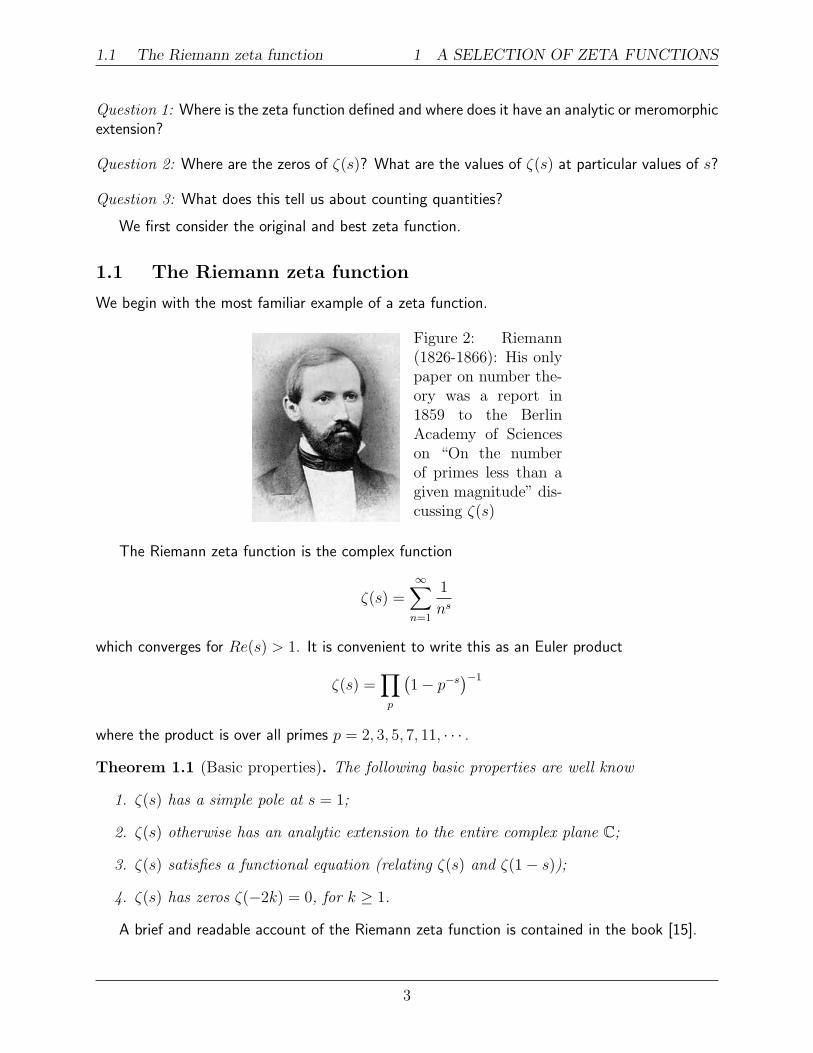
We begin with the most familiar example of a zeta function.

Figure 2: Riemann(1826-1866): His onlypaper on number the-ory was a report in1859 to the BerlinAcademy of Scienceson “On the numberof primes less than agiven magnitude” dis-cussing ζ(s)

The Riemann zeta function is the complex function

ζ(s) =∞∑n=1

1

ns

which converges for Re(s) > 1. It is convenient to write this as an Euler product

ζ(s) =∏p

(1− p−s

)−1

where the product is over all primes p = 2, 3, 5, 7, 11, · · · .

Theorem 1.1 (Basic properties). The following basic properties are well know

1. ζ(s) has a simple pole at s = 1;

2. ζ(s) otherwise has an analytic extension to the entire complex plane C;

3. ζ(s) satisfies a functional equation (relating ζ(s) and ζ(1− s));

4. ζ(s) has zeros ζ(−2k) = 0, for k ≥ 1.

A brief and readable account of the Riemann zeta function is contained in the book [15].

3

1.2 Other zeta functions 1 A SELECTION OF ZETA FUNCTIONS

1.2 Other zeta functions

Let us recall a few other well known zeta functions.

Example 1.2 (Weil zeta function from number theory). Let X be a (n-dimensional) projec-tive algebraic variety over the field Fq with q elements. Let Fqm be the degree m extension ofFq and let Nm denote the number of points of X defined over Fqm. We define a zeta functionby

ζX(s) = exp

(∞∑m=1

Nm

m(q−s)m

).

For the particular case of the projective line we have that Nm = qm + 1 and ζ(s) = 1/(1 −q−s)(1− q1−s). The reader can fine more details in [7].

Theorem 1.3 (Weil Conjectures: Grothendeick-Dwork-Deligne). The function ζX(s) is ra-tional in qs. We can write ζX(s) =

∏2ni=0 Pi(q

−s)(−1)iwhere Pi(·) are polynomials and the

zeros ζX(s) of occur where Re(s) = k2.

An important ingredient of the above theory is a version of the Lefschetz fixed point theorem.The original version of the Lefschetz fixed point theorem can also be used to study another zetafunction.

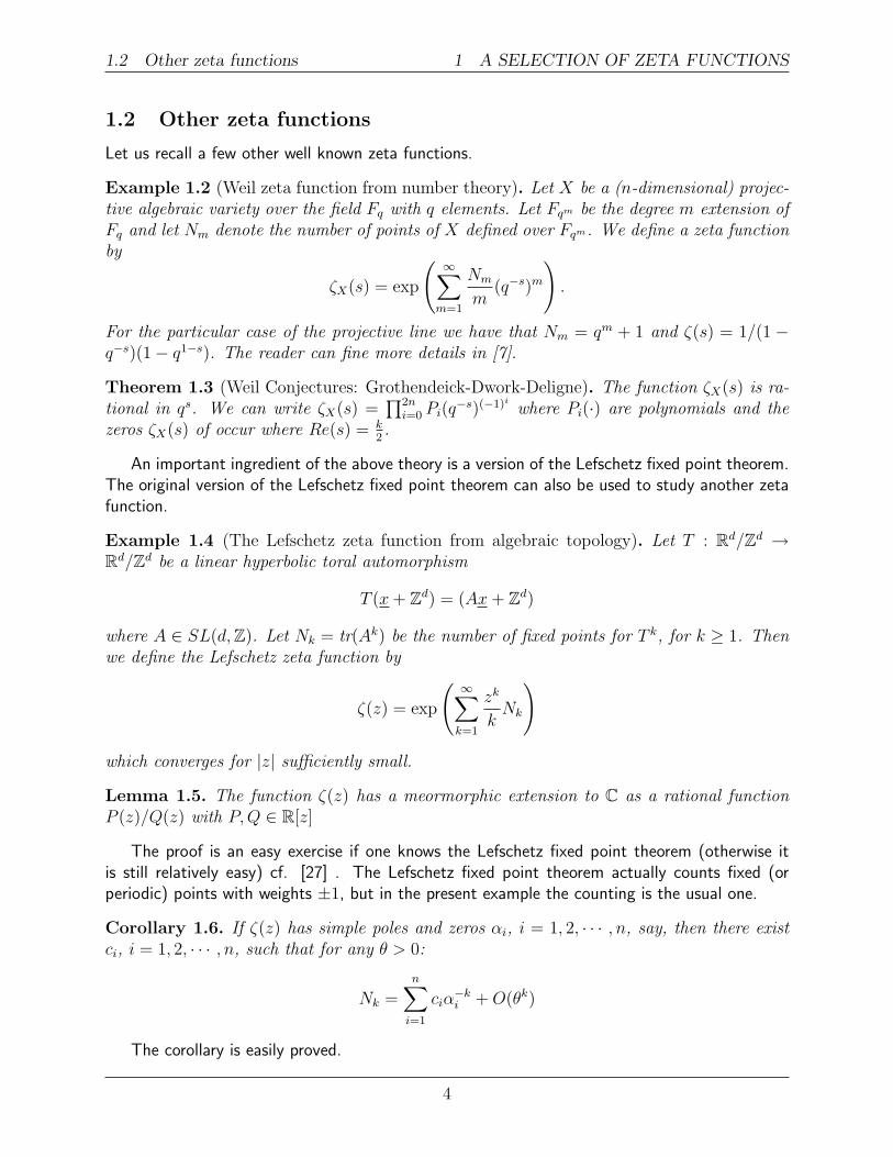
Example 1.4 (The Lefschetz zeta function from algebraic topology). Let T : Rd/Zd →Rd/Zd be a linear hyperbolic toral automorphism

T (x+ Zd) = (Ax+ Zd)

where A ∈ SL(d,Z). Let Nk = tr(Ak) be the number of fixed points for T k, for k ≥ 1. Thenwe define the Lefschetz zeta function by

ζ(z) = exp

(∞∑k=1

zk

kNk

)

which converges for |z| sufficiently small.

Lemma 1.5. The function ζ(z) has a meormorphic extension to C as a rational functionP (z)/Q(z) with P,Q ∈ R[z]

The proof is an easy exercise if one knows the Lefschetz fixed point theorem (otherwise itis still relatively easy) cf. [27] . The Lefschetz fixed point theorem actually counts fixed (orperiodic) points with weights ±1, but in the present example the counting is the usual one.

Corollary 1.6. If ζ(z) has simple poles and zeros αi, i = 1, 2, · · · , n, say, then there existci, i = 1, 2, · · · , n, such that for any θ > 0:

Nk =n∑i=1

ciα−ki +O(θk)

The corollary is easily proved.

4


Exercise 1.7. Derive the Corollary from the Lemma.

Question 1.8. What happens if the poles or zeros are not necessarily simple?

We recall an exam question from Warwick University.

Exercise 1.9 (Example from MA424 exam (Warwick, May 2010)). Compute the zeta func-tion for the hyperbolic toral automorphism T : R2/Z2 → R2/Z2 associated to

A =

(2 11 1

).

Solution: In this case Nm = tr(Am)− 2, for m ≥ 1. Thus

ζ(z) = exp

(∞∑m=1

zm

m(tr(Am)− 2)

)=

1− 2z

det(I − zA).

This is a rational function ζ(z) = 1−2z2z2−3z

.

It would appropriate here to mention also the Milnor-Thurston zeta function (and kneadingmatrices) [13] and the Hofbauer-Keller zeta function for interval maps [5]. Finally, we recall athird type of zeta function.

Example 1.10 (Artin Mazur zeta function for Subshifts of finite type). Let σ : ΣA → ΣA

be a mixing subshift of finite on the space of sequences

ΣA = {x = (xn) ∈ {1, · · · , k}Z : A(xn, xn+1) = 1 for n ∈ Z}

where A is a k×k aperiodic matrix with entries either 0 or 1. Let Nk = tr(Ak) be the numberof periodic points of period k. Then we define a discrete zeta function by

ζ(z) = exp

(∞∑k=1

zk

kNk

)

which converges for |z| sufficiently small. In this case, the following is a simple, but funda-mental, result [2].

Lemma 1.11. The function ζ(z) has a meormorphic extension to C as the reciprocal of apolynomial, i.e., ζ(z) = 1/ det(I − zA).

This follows easily by expressing the periodic points in terms of the traces tr(An) of the powersAn.

Exercise 1.12. Prove the Lemma.

Using this lemma we can easily compute explicitly the zeta functions.

5


Exercise 1.13. Compute the zeta function for the hyperbolic toral automorphism of R2/Z2

associated to

A =

(2 11 1

)Corollary 1.14. If A has simple eigenvalues αi, i = 1, 2, · · · , k, say, then there exist ci,i = 1, 2, · · · , k, such that for any θ > 0:

Nk =k∑i=1

ciα−ki +O(θk)

This follows by considering the power series expansions.

Exercise 1.15. Derive the Corollary from the Lemma.

We recall another exam question from Warwick University.

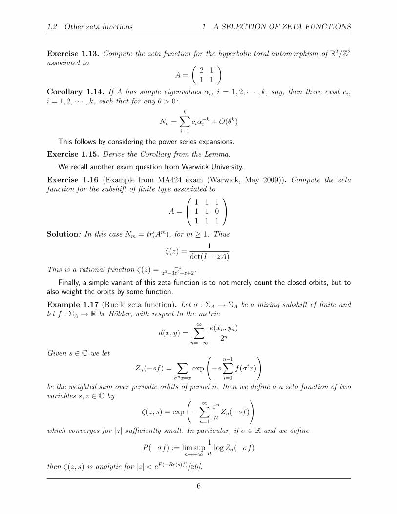
Exercise 1.16 (Example from MA424 exam (Warwick, May 2009)). Compute the zetafunction for the subshift of finite type associated to

A =

1 1 11 1 01 1 1

Solution: In this case Nm = tr(Am), for m ≥ 1. Thus

ζ(z) =1

det(I − zA).

This is a rational function ζ(z) = −1z3−3z2+z+2

.

Finally, a simple variant of this zeta function is to not merely count the closed orbits, but toalso weight the orbits by some function.

Example 1.17 (Ruelle zeta function). Let σ : ΣA → ΣA be a mixing subshift of finite andlet f : ΣA → R be Holder, with respect to the metric

d(x, y) =∞∑

n=−∞

e(xn, yn)

2n

Given s ∈ C we let

Zn(−sf) =∑σnx=x

exp

(−s

n−1∑i=0

f(σix)

)be the weighted sum over periodic orbits of period n. then we define a a zeta function of twovariables s, z ∈ C by

ζ(z, s) = exp

(−∞∑n=1

zn

nZn(−sf)

)which converges for |z| sufficiently small. In particular, if σ ∈ R and we define

P (−σf) := lim supn→+∞

1

nlogZn(−σf)

then ζ(z, s) is analytic for |z| < eP (−Re(s)f)[20].

6

2 SELBERG ZETA FUNCTION

Lemma 1.18. There exists 0 < θ < 1 such that ζ(z, s) has a meromorphic extension to|z| < eP (−Re(s)f)/θ.

A particularly illuminating example is where the function is locally constant.

Exercise 1.19. Let f : ΣA → R depend only on the zeroth and first coordinates x0 andx1 (i.e., f(x) = f(x0, x1)). How does one write ζ(z, s) in terms of the matrix As =(A(i, j)e−sf(i,j))?

In the particular case that f is identically zero, we recover the Artin-Mazer zeta function.The Ruelle zeta function is a useful bridge between certain zeta functions for flows and those

for discrete maps. We will return to this when we discuss suspension flows. However, in order togive a more coherent presentation we will typically present the Ruelle zeta function in the contextof geodesic flows for surfaces of variable negative curvature, giving a natural generalization ofthe Selberg zeta function for surfaces of constant negative curvature.

2 Selberg Zeta function

A particularly important zeta function in both analysis and geometry is the Selberg zeta function.A comprehensive account appears in [6]. A lighter account appears in [28].

2.1 Definition: Hyperbolic geometry and closed geodesics

Perhaps one of the easier routes into understanding dynamical zeta functions for flows is viageometry. Assume that V is a compact surface with constant curvature κ = −1.

Figure 3: The upperhalf plane H2 with thePoincare metric. Inthis Escher picture thecreatures are the samesize, with respect to thePoincare metric. Theyonly seem smaller as weapproach the boundary inthe Euclidean metric.

The covering space is the upper half plane H2 = {z = x + iy : y > 0} with the Poincaremetric

ds2 =dx2 + dy2

y2

(with constant curvature κ = −1). In particular, compared with the usual Euclidean distance, thedistance in the Poincare metric tends to infinity as y tends to zero, to the extent that geodesicsnever actually reach the boundary.

7

2.1 Definition: Hyperbolic geometry and closed geodesics2 SELBERG ZETA FUNCTION

Lemma 2.1. There are a countable infinity of closed geodesics.

Proof. There is a one-one correspondence between closed geodesics and conjugacy classes inthe fundamental group π1(V ). The group π1(V ) is finitely generated and countable, as areits conjugacy classes.

We denote by γ one of the countably many closed geodesics on V . We can write l(γ) for thelength of γ. We can also interpret the closed geodesics dynamically.

Hyperbolic Upper Half Plane

V

Geodesic

Geodesic

Figure 4: The upper half plane H2 isthe universal cover for V . Geodesicson the upper half plane H2 projectdown to geodesics on V . Sometimesthey may be closed geodesics.

Example 2.2 (Geodesic flow). Let V be a compact surface with curvature κ = −1, forx ∈ V . Let

M = SV = {(x, v) ∈ TM : ‖v‖x = 1}denote the unit tangent bundle. then we let φt : M → M be the geodesic flow, i.e., φt(v) =γ(t) where γ : R→ V is the unit speed geodesic with γ(0) = (x, v).

This also corresponds to parallel transporting tangent vectors along geodesics.

xv

γv

φt(v)

x v = ! t (v)

Figure 5: Periodic orbits for the geodesic flow correspond to closed geodesics on surface V .

We now come to the definition of the zeta function.

Definition 2.3. The Selberg zeta function is a function of s ∈ C formally defined by

Z(s) =∞∏n=0

∏γ

(1− e−(s+n)l(γ)

).

8

3 RIEMANN HYPOTHESIS

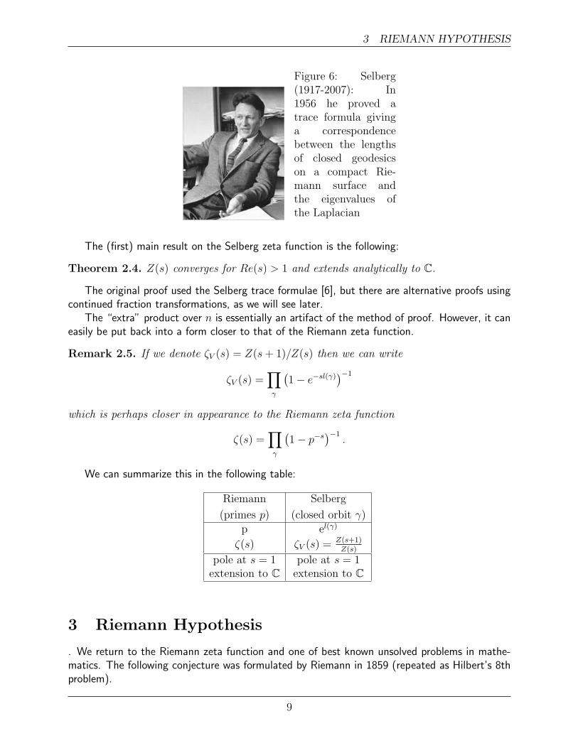
Figure 6: Selberg(1917-2007): In1956 he proved atrace formula givinga correspondencebetween the lengthsof closed geodesicson a compact Rie-mann surface andthe eigenvalues ofthe Laplacian

The (first) main result on the Selberg zeta function is the following:

Theorem 2.4. Z(s) converges for Re(s) > 1 and extends analytically to C.

The original proof used the Selberg trace formulae [6], but there are alternative proofs usingcontinued fraction transformations, as we will see later.

The “extra” product over n is essentially an artifact of the method of proof. However, it caneasily be put back into a form closer to that of the Riemann zeta function.

Remark 2.5. If we denote ζV (s) = Z(s+ 1)/Z(s) then we can write

ζV (s) =∏γ

(1− e−sl(γ)

)−1

which is perhaps closer in appearance to the Riemann zeta function

ζ(s) =∏γ

(1− p−s

)−1.

We can summarize this in the following table:

Riemann Selberg

(primes p) (closed orbit γ)

p el(γ)

ζ(s) ζV (s) = Z(s+1)Z(s)

pole at s = 1 pole at s = 1extension to C extension to C

3 Riemann Hypothesis

. We return to the Riemann zeta function and one of best known unsolved problems in mathe-matics. The following conjecture was formulated by Riemann in 1859 (repeated as Hilbert’s 8thproblem).

9

3 RIEMANN HYPOTHESIS

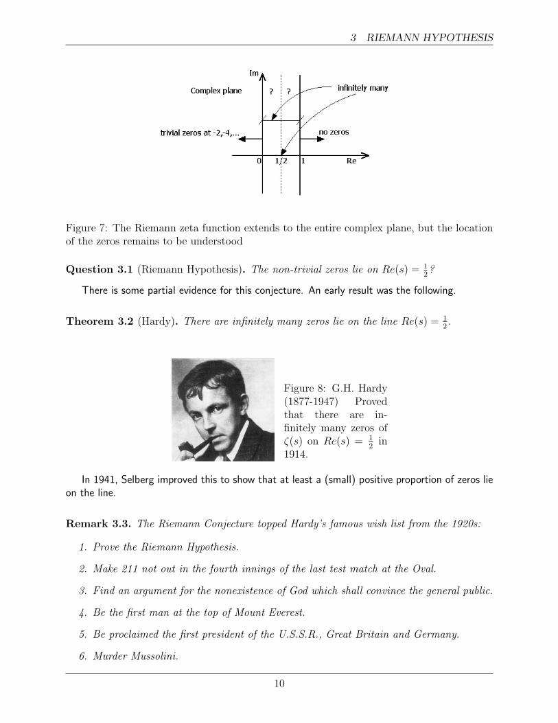
Figure 7: The Riemann zeta function extends to the entire complex plane, but the locationof the zeros remains to be understood

Question 3.1 (Riemann Hypothesis). The non-trivial zeros lie on Re(s) = 12?

There is some partial evidence for this conjecture. An early result was the following.

Theorem 3.2 (Hardy). There are infinitely many zeros lie on the line Re(s) = 12.

Figure 8: G.H. Hardy(1877-1947) Provedthat there are in-finitely many zeros ofζ(s) on Re(s) = 1

2in

1914.

In 1941, Selberg improved this to show that at least a (small) positive proportion of zeros lieon the line.

Remark 3.3. The Riemann Conjecture topped Hardy’s famous wish list from the 1920s:

1. Prove the Riemann Hypothesis.

2. Make 211 not out in the fourth innings of the last test match at the Oval.

3. Find an argument for the nonexistence of God which shall convince the general public.

4. Be the first man at the top of Mount Everest.

5. Be proclaimed the first president of the U.S.S.R., Great Britain and Germany.

6. Murder Mussolini.

10

3.1 The Hilbert-Polya approach to the Riemann hypothesis3 RIEMANN HYPOTHESIS

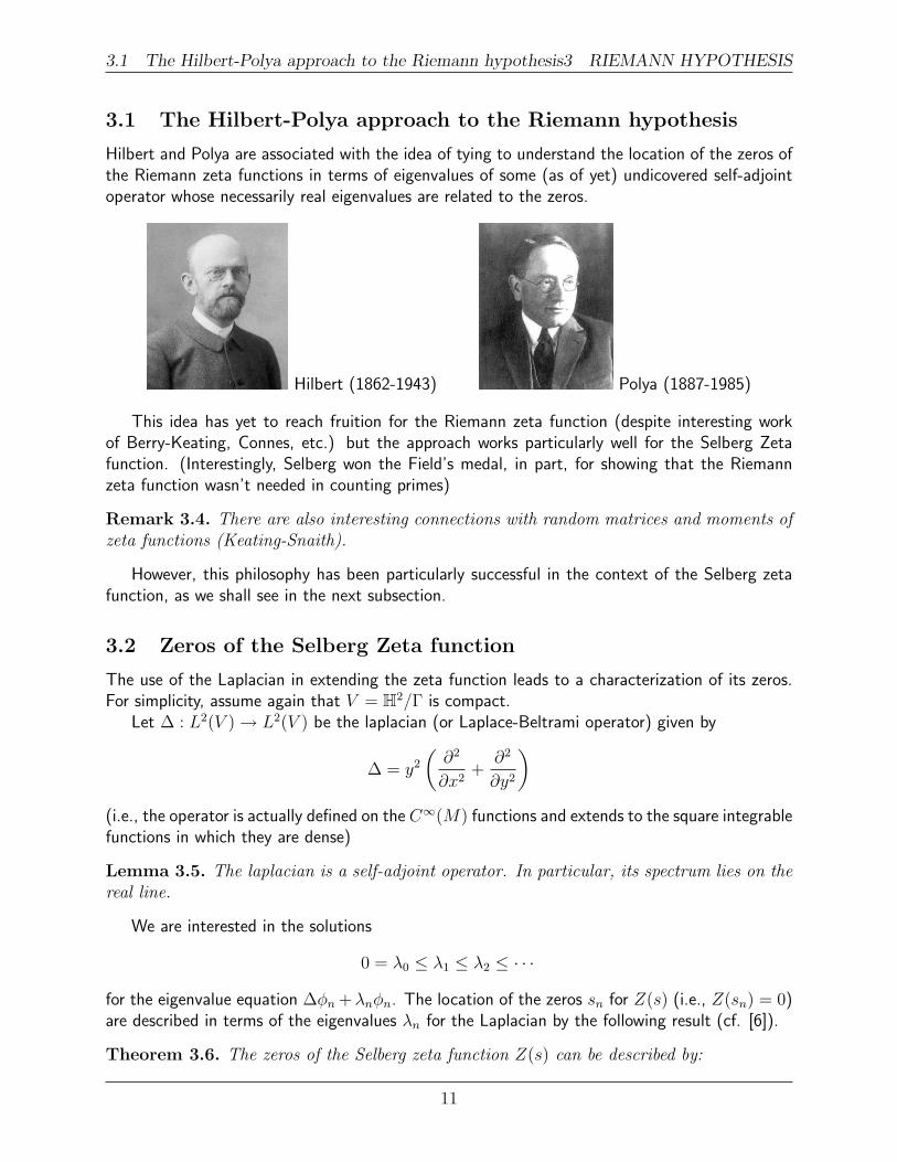
3.1 The Hilbert-Polya approach to the Riemann hypothesis

Hilbert and Polya are associated with the idea of tying to understand the location of the zeros ofthe Riemann zeta functions in terms of eigenvalues of some (as of yet) undicovered self-adjointoperator whose necessarily real eigenvalues are related to the zeros.

Hilbert (1862-1943) Polya (1887-1985)

This idea has yet to reach fruition for the Riemann zeta function (despite interesting workof Berry-Keating, Connes, etc.) but the approach works particularly well for the Selberg Zetafunction. (Interestingly, Selberg won the Field’s medal, in part, for showing that the Riemannzeta function wasn’t needed in counting primes)

Remark 3.4. There are also interesting connections with random matrices and moments ofzeta functions (Keating-Snaith).

However, this philosophy has been particularly successful in the context of the Selberg zetafunction, as we shall see in the next subsection.

3.2 Zeros of the Selberg Zeta function

The use of the Laplacian in extending the zeta function leads to a characterization of its zeros.For simplicity, assume again that V = H2/Γ is compact.

Let ∆ : L2(V )→ L2(V ) be the laplacian (or Laplace-Beltrami operator) given by

∆ = y2

(∂2

∂x2+

∂2

∂y2

)(i.e., the operator is actually defined on the C∞(M) functions and extends to the square integrablefunctions in which they are dense)

Lemma 3.5. The laplacian is a self-adjoint operator. In particular, its spectrum lies on thereal line.

We are interested in the solutions

0 = λ0 ≤ λ1 ≤ λ2 ≤ · · ·

for the eigenvalue equation ∆φn +λnφn. The location of the zeros sn for Z(s) (i.e., Z(sn) = 0)are described in terms of the eigenvalues λn for the Laplacian by the following result (cf. [6]).

Theorem 3.6. The zeros of the Selberg zeta function Z(s) can be described by:

11

4 DYNAMICAL APPROACH

1. s = 1 is a zero.

2. sn = 12± i√

14− λn, for n ≥ 1, are “spectral zeros”.

3. s = −m, for m = 0, 1, 2, · · · , are “trivial zeros”.

0 1

Re(s) = 1/2

Figure 9: Spectral zeros ofthe Selberg Zeta functionThe spectral zeros lie onthe “cross” [0, 1] ∪ [1

2−

i∞, 12

+ i∞].

Remark 3.7. A somewhat easier setting for studying Laplacians is on the standard flattorus Td = Rd/Zd. When d = 1 then ∆ = d2

dx2 and self-adjointness is essentially integrationby parts, i.e.,

∫(∆ψ)φdx =

∫ψ(∆φ)dx, the eigenvalues are {n2} and the eigenfunctions are

ψnm(x, y) = e2πinx. When d = 2 then ∆ = ∂2

∂x2 + ∂2

∂x2 then the eigenvalues are {n2 +m2} andthe eigenfunctions are ψnm(x, y) = e2πi(nx+my).

Remark 3.8. The asymptotic estimate on growth eigenvalues of the Laplace operator comesfrom Weyl’s theorem.

The proof of these results is usually based on using the Selberg trace formula to extend thelogarithmic derivative Z ′(s)/Z(s) [6]. In an appendix we outline the strategy to proving thetheorem.

If V is non-compact, but of finite area (such as the modular surface), then there are extra zeroswhich correspond to those for the Riemann zeta function. In view of the Riemann hypothesis,this illustrates the difficulty is understanding the zeros in that case.

4 Dynamical approach

We would like to use a more dynamical approach to study the Selberg zeta function. This allowsus to recover some of the classical results (such as the existence of an analysic extension to C)and this different perspective also allows us to get additional bounds on the zeta function. Withthis perspective, the ideas are a little clearer if we study the special case of the Modular surface.

We begin with a little motivation for this viewpoint, which includes a connection betweenclosed geodesic for the Modular flow and periodic points for the continued fraction transformation.

12

4.1 Binary Quadratic forms 4 DYNAMICAL APPROACH

4.1 Binary Quadratic forms

Let us begin with a simple connection between closed geodesics and number theory. Considerquadratic forms

Q(x, y) = Ax2 +Bxy + Cy2

where A,B,C ∈ Z.

Definition 4.1. Two quatratic forms Q1(x, y) and Q2(x, y) are said to be equivalent if thereexist α, β, γ, δ ∈ Z with αδ − βγ = 1 and Q1(x, y) = Q2(αx+ βy, γx+ δy).

A fundamental quantity in number theory is that of the Class Number. We recall the definition.

Definition 4.2. Given d > 0, the class number h(d) is the number of inequivalent quadraticforms with given discriminant d := B2 − 4AC.

There is a correspondence between equivalence classes of quadratic forms and closed geodesics.In particular, the distinct roots x, x′ of Ax2 +Bx+C = 0 determine a unique a unique geodesicγ on H2 with γ(+∞) = x and γ(−∞) = x′ which quotients down to a closed geodesic γ on V .

1/2 0 1/2 1−11/2 0 1/2 1−1γ(− ) γ(+ )8 8

V

Figure 10: Geodesics on the Poincar’e upper half plane are determined by their two end-points. Moreover, they project down to geodesics on the Modular surface. Of particularinterest is when this image geodesic is closed.

On the other hand, the group PSL(2,Z) = SL(2,Z)/{±I} acts isometrically on H2 as linearfractional transformations, i.e.,

g =

(a bc d

)acts by g : z 7→ az + b

cz + d.

The quotient space V = H2/PSL(2,Z) is the modular surface.The following result dates back to Sarnak [25].

Lemma 4.3. Equivalence classes [Q] of quadratic forms Q(x, y) = Ax2 + Bxy + Cy2 (ofdiscriminant d) correspond to closed geodesics γ of length

l(γ) = 2 log

(t+ u

√d

2

).

where t2 − du2 = 4 and (t, u) is a fundamental solution. The class number h(d) correspondsthe multiplicity of distinct closed geodesics with the same length.

13

4.2 Discrete transformations 4 DYNAMICAL APPROACH

Of course, the lengths are constrained by the fact that el(γ) + e−l(γ) ∈ Z+ (since it is thetrace of an element of SL(2,Z)).

Exercise 4.4. Show that closed geodesics can have a high multiplicity.

Remark 4.5. Gauss observed that the dependence h(d) on d is very irregular. Siegel showedthat: ∑

d∈D,d≤x

h(d) log εd ∼π2x3/2

18ζ(3)as x→ +∞.

However, using the above correspondence Sarnak [25] gave an asymptotic formula for sumsof class numbers:

1

Card({d ∈ D : εd ≤ x})∑

{d∈D : εd≤x}

h(d) ∼ 8

35

x

2 log xas x→ +∞.

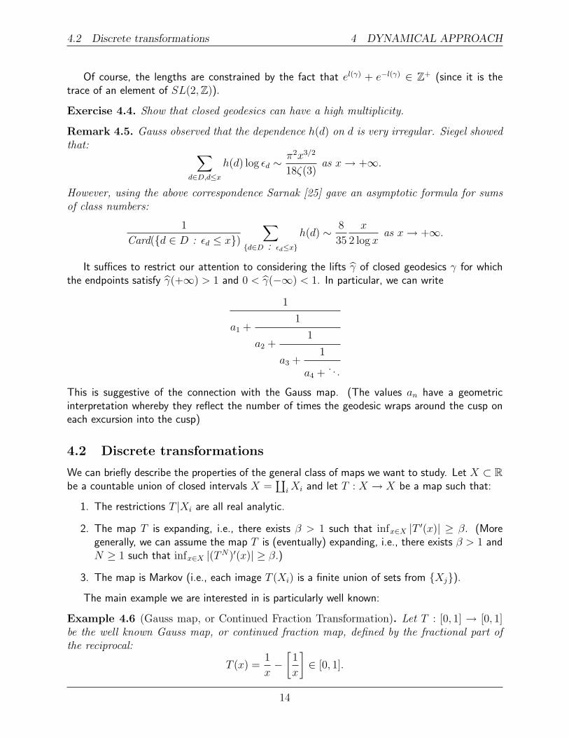
It suffices to restrict our attention to considering the lifts γ of closed geodesics γ for whichthe endpoints satisfy γ(+∞) > 1 and 0 < γ(−∞) < 1. In particular, we can write

1

a1 +1

a2 +1

a3 +1

a4 +. . .

This is suggestive of the connection with the Gauss map. (The values an have a geometricinterpretation whereby they reflect the number of times the geodesic wraps around the cusp oneach excursion into the cusp)

4.2 Discrete transformations

We can briefly describe the properties of the general class of maps we want to study. Let X ⊂ Rbe a countable union of closed intervals X =

∐iXi and let T : X → X be a map such that:

1. The restrictions T |Xi are all real analytic.

2. The map T is expanding, i.e., there exists β > 1 such that infx∈X |T ′(x)| ≥ β. (Moregenerally, we can assume the map T is (eventually) expanding, i.e., there exists β > 1 andN ≥ 1 such that infx∈X |(TN)′(x)| ≥ β.)

3. The map is Markov (i.e., each image T (Xi) is a finite union of sets from {Xj}).

The main example we are interested in is particularly well known:

Example 4.6 (Gauss map, or Continued Fraction Transformation). Let T : [0, 1] → [0, 1]be the well known Gauss map, or continued fraction map, defined by the fractional part ofthe reciprocal:

T (x) =1

x−[

1

x

]∈ [0, 1].

14


(We ignore the complication with the point 0, in the great tradition of ergodic theory). Inthis example X =

∐nXn where Xn = [ 1

n+1, 1n]. In particular,

T ′(x) = − 1

x2

and we can check that T is eventually expanding since |(T 2)′(x)| ≥ 4. Furthermore, for eachXi we have TXi = [0, 1] = X confirming the Markov proprty.

Lemma 4.7 (Artin, Hedlund, Series [26]). There is a bijection between the periodic orbitsof T (of even period) and the closed geodesics for H2/Γ where Γ = PSL(2,Z).

A natural generalization of the Gauss map is the following.

Example 4.8 (Hurewicz-Nakada Continued fractions). We can first consider the HurewiczContinued fraction maps f :

[−1

2, 1

2

]→[−1

2, 1

2

]before by

f(x)− 1

x− 〈−1

x〉

where 〈ξ〉 is the nearest integer to ξ cf. [3]. More generally, for q = 4, 5, 6 · · · , let λq =2 cos(π/q). We define

f :

[−λq

2,λq2

]→[−λq

2,λq2

]by

f(x) = −1

x− 1

x〈−1

x〉qλq

where 〈ξ〉q := [ξ/λq + 1/2].

Lemma 4.9 (Mayer and Muhlenbruch). There is a bijection between the periodic orbits off and the closed geodesics for H2/Γ where Γ = 〈S, Tq〉 is the Hecke group generated by

S =

(0 −11 0

)and Tq =

(1 λq0 1

).

Let us next consider a different type of generalization of the Modular surfaces and the con-tinued fraction transformation.

Example 4.10 (Principle congruence subgroups). For each N ≥ 1 we can consider thesubgroups Γ(N) < PSL(2,Z) such that

Γ(N) = {A ∈ PSL(2,Z) : A = I (mod N)}.

The geodesic flow on H2/Γ(N) is a finite extension of the geodesic flow on the modularsurface with the finite group

G := Γ/Γ(N) = SL(2,Z/NZ).

The new transformation is a skew product over the continued fraction map: T : [0, 1]×G→[0, 1]×G, i.e., T (x, g) = (Tx, g(x)g) where g : [0, 1]→ G.

15


Lemma 4.11 (Chung-Mayer, Kraaikamp-Lopes). There is a bijection between the periodic

orbits of T and the closed geodesics for H2/Γ(N).

One can also consider higher dimensional analogues of continued fraction transformations[22]. Let X ⊂ Rd be a subset of Euclidean space and let X =

∐iXi be a union of sets (where

intXi ∩ intXj = ∅ and Xi = cl(intXi)). Let T : X → X be a map such that:

1. The restrictions Ti = T |Xi are real analytic.

2. The map T is expanding, i.e., there exists β > 1 such that ‖DT (v)‖/‖v‖ ≥ β.

3. The map is Markov (i.e., the image Ti(Xi)) is a finite unions of sets from {Xi}

The following example is useful in studying both Interval Exchange Transformations andTeichmuller flows for translation surfaces.

Example 4.12 (Rauzy-Veech-Zorich). Let us consider a continued fraction transformationon a finite union of copies of the (n − 1)-dimensional simplicies ∆. Let R be (a subset of)the permutations on k-symbols and partition ∆×R = ∪π∈R∆+

π ∪∆−π where

∆+π = {(λ, π) ∈ ∆× {π} : λn > λπ−1n} and ∆−π = {(λ, π) ∈ ∆× {π} : λn < λπ−1n}

(up to a set of zero measure). Define a map T0 : ∆×R → ∆×R by

T0(λ, π) =

(

(λ1,··· ,λn−1,λn−λk)1−λk

, aπ)

if λ ∈ ∆−π((λ1,··· ,λk−1,λk−λn,λn,λk+1,··· ,λn−1)

1−λn, bπ)

if λ ∈ ∆+π

where aπ and bπ are suitably defined new permutations Actually, this doesn’t quite satisfy theexpansion assumption and so one accelerate the map following Zorich, Bufetov and Marmi-Yoccoz, etc.

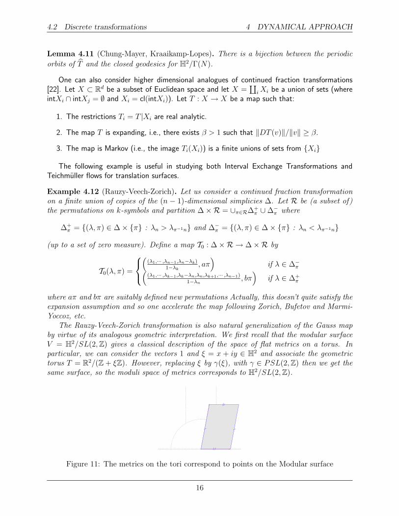
The Rauzy-Veech-Zorich transformation is also natural generalization of the Gauss mapby virtue of its analogous geometric interpretation. We first recall that the modular surfaceV = H2/SL(2,Z) gives a classical description of the space of flat metrics on a torus. Inparticular, we can consider the vectors 1 and ξ = x + iy ∈ H2 and associate the geometrictorus T = R2/(Z + ξZ). However, replacing ξ by γ(ξ), with γ ∈ PSL(2,Z) then we get thesame surface, so the moduli space of metrics corresponds to H2/SL(2,Z).

Figure 11: The metrics on the tori correspond to points on the Modular surface

16

4.3 Suspension flows 4 DYNAMICAL APPROACH

More generally, we can replace the torus by a surface of higher genus with a flat met-ric (i.e., translation surfaces). Then the continued fraction transformation is replaced bythe Rauzy-Veech-Zorich transformation, which encodes orbits for an associated flow (the Te-ichmuller flow). Actually, this doesn’t quite satisfy all of the properties we might want, and soone modify the map (essentially by inducing) following ideas of Bufetov or Marmi-Moussa-Yoccoz, etc.

The associated zeta function is clearly related (in a way which is still not well understood)to the closed geodesics for the Teichmuller flow on the space of translation surfaces (by analogywith the geodesic flow on the Modular surface).

Exercise 4.13. Is there a connection with the asymptotic results of Athreya-Bufetov-Eskin-Mirzakhani for Teichmuller space?

When one discusses higher dimensional continued fraction transformations, it is natural tomention the most famous example:

Example 4.14 (Jacobi-Perron). We can define this two dimensional analogue T : [0, 1]2 →[0, 1]2 of the Gauss map by

T (x, y) =

(y

x−[yx

],

1

x−[

1

x

]).

Unfortunately, it isn’t clear at the present time how the zeta function gives interesting insightsinto this map (e.g., the invariant density, which isn’t explicitly known, or the Lyapunovexponents).

4.3 Suspension flows

A basic construction in ergodic theory is to associate to any discrete transformation a flow onthe area under the graph of a suitable positive function. This flow is called the suspension flow(or special flow). More precisely, given a function r : X → R+ we define a new space by

Y = {(x, u) ∈ X × R : 0 ≤ u ≤ r(x)}

with the identification of (x, r(x)) with (T (x), 0). The (semi)-flow is defined on the space Ylocally by ψt(x, u) = (x, u+ t), subject to the identification, i.e,

ψt(x, u) = (T nx, t+ u−n−1∑i=0

r(T ix)) where 0 ≤ t+ u−n−1∑i=0

r(T ix)) ≤ r(x).

In the present context, a natural choice of function is given by r(x) = log |T ′(x)| (or, moregenerally, in higher dimensions r(x) = log |Jac(T )(x)|).

Lemma 4.15. If r(x) = log |T ′(x)| then the flow ψ has entropy h(ψ) = 1 and the measureof maximum entropy is absolutely continuous.

This is a simple exercise using the variational principle for pressure [14].

17

4.4 Transfer operators 4 DYNAMICAL APPROACH

Exercise 4.16. Prove the lemma.

We can now apply this to the continued fraction transformation.

Example 4.17. The primary example is the continued fraction transformation T (x) = {1/x}and then T ′(x) = 1/x2 and thus r(x) = −2 log x.

4.4 Transfer operators

In order to extend the domain of the zeta function by dynamical methods it is convenient tointroduce a family of bounded linear operators.

Definition 4.18. Given T : X → X and s ∈ C we can associate the transfer operatorLs : C0(X)→ C0(X) by

Lh(x) =∑

T (Xi)⊃Xj

|Jac(DTi)(x)|sf(Tix) where x ∈ Xj

provided the series converges.

We want to consider a smaller space of functions, in order that the spectrum should besufficiently small to proceed further. To begin, assume that we choose a complex neighbourhoodU ⊃ X. We can then consider the space of analytic functions h : U → C which are analyticand bounded. This forms a Banach space, which we denote by A(U) with the supremum norm‖ · ‖∞.

Definition 4.19. We recall that a nuclear operator L (or order zero) is one for which thereare families of functions wn ∈ A(U) and functionals ln ∈ A(U)∗ (with ‖wn‖ = 1 = ‖ln‖)such that

L(·) =∞∑n=0

αnwnln(·).

where |αn| = O(θn), for some 0 < θ < 1.In the case that there are only finitely many branches we have the following result of Ruelle

[23].

Lemma 4.20 (Ruelle). Assume that whenever T (Xi) ⊃ Xj we have that the closure of theimage Ti(U) is contained in U . It then follows that each operator Ls : A(U) → A(U) asdefined above is nuclear.

The easiest way to understand this lemma is through considering simple examples. The basicidea can be seen in the following.

Exercise 4.21. Let U = {z ∈ C : |z| < 1} and let |λ| < 1. By considering the power seriesexpansion about z = 0 that the operator M : A(U) → A(U) defined by Mf(z) = f(λz) isnuclear.

In particular, nuclear operators have countably many eigenvalues and are trace class. We cannow use the following result:

18

4.4 Transfer operators 4 DYNAMICAL APPROACH

Lemma 4.22 (Grothendeick). We can write

det(I − zL) = exp

(−∞∑n=1

zn

ntr(Lns )

)

Moreover, we have the following characterizations of the traces due to Ruelle [23].

Lemma 4.23 (Ruelle). We have the following:

1. The trace of Ls : A(U)→ A(U) is

tr(Ls) =∑Tx=x

|Jac(DT )(x)|−s

det(I −DxT−1).

2. For each n ≥ 1 the trace of Lns : A(U)→ A(U) is

tr(Lns ) =∑Tx=x

|Jac(DT )(x)|−s

det(I −Dx(T n)−1).

Of particular interest is the one dimensional case.

Corollary 4.24. In the particular case that X is one dimensional we have that:

tr(Ls) =∑Tx=x

|T ′(x)|−s

det(I − (T ′(x))−1

Of particular interest is the special case of the continued fraction transformation, which wasstudied by Mayer [11].

Example 4.25 (Mayer). Consider the Gauss map T : [0, 1]→ [0, 1] is defined by

T (x) =1

x−[

1

x

]Let U = {z ∈ : |z − 1| < 3

2} then we can write

Lsw(z) =∞∑n=1

1

(z + n)2sw

(1

z + n

)for w ∈ A(U) . In particular, we can write Ls =

∑∞n=1 Ln,s where

Ls,nw(z) =1

(z + n)2sw

(1

z + n

)are again trace class, and thus tr(Ls) =

∑∞n=1 tr(Ln,s). We can solve the eigenfunction

equation Ls,nw(z) = λw(z) to deduce that the eigenvalues are {(zn + n)−2s+2m : m ≥ 0}where zn satisfies 1/(zn + n) = zn, i.e., zn = [n] (as a periodic continued fraction). This is

19

4.5 Zeta functions for the Modular surface 4 DYNAMICAL APPROACH

achieved by evaluating both sides at the fixed point, and differentiating if w is zero at thispoint. Thus we can write

tr(Ln,s) =[n]2s

1− [n]2and tr(Ls) =

∞∑n=1

[n]2s

1− [n]2.

More generally, we can write

tr(Lks) =∞∑

a1,··· ,ak=1

[a1, · · · , ak]2s

1− [a1, · · · , ak]2.

Exercise 4.26. Confirm these formulae for the eigenvalues and tr(Lks).

The following question is of a more general nature.

Question 4.27. Let Γ be any geometrically finite Fuchsian group. Can we expect to usecoding of the dynamics on the boundary as in [26] to give a functional equation characterizingthe zeros of the Selberg zeta function?

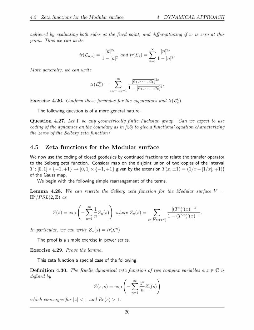
4.5 Zeta functions for the Modular surface

We now use the coding of closed geodesics by continued fractions to relate the transfer operatorto the Selberg zeta function. Consider map on the disjoint union of two copies of the intervalT : [0, 1]×{−1,+1} → [0, 1]×{−1,+1} given by the extension T (x,±1) = (1/x− [1/x],∓1))of the Gauss map.

We begin with the following simple rearrangement of the terms.

Lemma 4.28. We can rewrite the Selberg zeta function for the Modular surface V =H2/PSL(2,Z) as

Z(s) = exp

(−∞∑n=1

1

nZn(s)

)where Zn(s) =

∑x∈Fix(Tn)

|(T n)′(x)|−s

1− (T 2n)′(x)−1.

In particular, we can write Zn(s) = tr(Ln)

The proof is a simple exercise in power series.

Exercise 4.29. Prove the lemma.

This zeta function a special case of the following.

Definition 4.30. The Ruelle dynamical zeta function of two complex variables s, z ∈ C isdefined by

Z(z, s) = exp

(−∞∑n=1

zn

nZn(s)

)which converges for |z| < 1 and Re(s) > 1.

20

4.6 General Principle 4 DYNAMICAL APPROACH

In particular, Z(1, s) = Z(s). For our purposes, we can think of the z terms as being a useful“book-keeping” device for keeping track of the periods with respect to T . One advantage of theRuelle dynamical zeta function formulation is that we can then formally expand

Z(z, s) = exp

(−∞∑n=1

zn

nZn(s)

)= 1 +

∞∑n=1

znan(s)

where a2n−1(s) = 0 and a2n(s) only depends on periodic points T of period ≤ 2n.

Theorem 4.31 (Ruelle). There exists c > 0 such that for each s there exists C > 0 suchthat |an(s)| ≤ Ce−cn

2. In particular, the series above converges for all s, z ∈ C.

Setting z = 1 recovers the Selberg zeta function for the Modular surface V .

Corollary 4.32. We have an expression for the Selberg zeta function

Z(s) = 1 +∞∑n=1

an(s)

which converges for all s ∈ C.

The dual characterization of the zeros of the Selberg zeta function in terms of the continuedfraction transformation and also the spectrum of the laplacian gives an interesting correspondencebetween the two. This bas been explored by Lewis and Zagier, and Mayer. More precisely, thecorrespondence between the spectral interpretation of the zeros and the use of the transferoperator leads to the study of analytic function on |z − 1| < 3

2satisfying

h(z)− h(z + 1) = (z)−2sh(1 + 1/z).

This is called a period function equation. We conclude with the following result.

Lemma 4.33. There is a bijection between zeros s = 1/2 + it for the Selberg zeta functionand the solutions for the period function equation in C− (−∞, 0] and the eigenfunctions ofthe laplacian with u(x) = 0(1/x).

These functions are closely related to the eigenfunctions of the laplacian called non-holomorphicmodular functions, or Maass wave forms.

4.6 General Principle

The dynamical method of extending the zeta function that we have described works for a varietyof other surfaces of constant negative curvature, where the continued fraction transformation isreplaced by other transformations. Typically, given a suitable surface we associate to a piecewiseanalytic expanding interval map T : I → I (replacing the continued fraction transformation) tothe group (replacing PSL(2,Z)).

We can then rewrite the Selberg zeta function as

Z(s) = 1 +∞∑n=1

an(s)

where

21

4.7 Dynamical approach to more general transformations and zeta functions4 DYNAMICAL APPROACH

1. an(s) only depends on periodic points T of period ≤ n;

2. There exists c > 0 such that for each s there exists C > 0 such that |an(s)| ≤ Ce−cn2. In

particular, the series converges for all s ∈ C.

The main conclusion is that we then have an expression for the Selberg zeta function

Z(s) = 1 +∞∑n=1

an(s)


4.7 Dynamical approach to more general transformations and zetafunctions

The versatility of this method is that it may be applied to more general situations than geodesicflows on surfaces. Given any suitable transformation T to which the underlying analysis applies,we can also associate a (suspension) flow and a zeta function.

For example, let X =∐∞

i=1 be a disjoint union of m-dimensional simplices Xi and letT : X → X be a map which:

1. Expand distances locally; and

2. T |Xi is analytic; and

3. is Markov (i.e., each image T (Xi) is a union of some of the other simplices).

We associate to an analytic expanding map T : I → I (replacing the continued fractiontransformation) the suspension flow under the graph of the function r : X → R+ defined byr(x) = log | det(DT )(x)|. We can then rewrite the Selberg zeta function as

Z(s) = 1 +∞∑n=1

an(s)

where

1. an(s) only depends on periodic points T of period ≤ n;

2. There exists c > 0 such that for each s there exists C > 0 such that |an(s)| ≤ Ce−cn(1+ 1

m).

In particular, the series converges for all s ∈ C.

We have an expression for the Selberg zeta function

Z(s) = 1 +∞∑n=1

an(s)


22

5 SPECIAL VALUES

We might then generalize the definition of the zeta function for the continued fraction trans-formation to:

Z(s) = exp

(−∞∑n=1

1

nZn(s)

)where Zn(s) =

∑x∈Fix(Tn)

| det(DT n)(x)|−s

det(I − (DT n)′(x)−1)

and we can conclude that Z(s) has an extension to C.

5 Special values

We return to the basic question of what information is provided by a knowledge of the extensionof the zeta function.

5.1 Special values: Determinant of the Laplacian

We would like to find a way to define a determinant “det(∆) =∏

n λn”. The basic complicationis that the sequence {λn} is unbounded and thus the product is undefined. In order to addressthis we first recall the following result on a slightly different complex function.

Lemma 5.1. The series

η(s) =∞∑n=1

λ−sn

has an analytic extension to the entire complex plane.

This extension now allows us to make the following definition.

Definition 5.2. We define the Determinant of the Laplacian by:

det(∆) = exp (−η′(0)) .

A nice introduction to these ideas is contained in [25].

Remark 5.3. Heuristically, one justifies the name by writing

“η′(0) = −∞∑n=1

(log λn)λ−sn |s=0 = −∞∑n=1

log λn.′′

The determinant has a direct connection with the Selberg zeta function:

Theorem 5.4. There exists C > 0 (depending only on the genus of the surface) such thatdet(∆) = CZ ′(1).

Sarnak, Wolpert and others have studied the smooth dependence of det(∆) on the choice ofmetric on the surface V . However, there appear to still remain questions about, say, the criticalpoints.

Conjecture 5.5 (Sarnak). There is a unique minimum for the determinant of the laplacianamong metrics of constant area.

23

5.2 Other special values: Resolvents and QUE 5 SPECIAL VALUES

5.2 Other special values: Resolvents and QUE

There is also an interesting connection between complex functions related to zeta functions andthe problem of Quantum Unique Ergodicity. We begin by describing a modification to the Selbergzeta function which carries information about a fixed reference function A.

Definition 5.6. Let A ∈ Cω(V ) with∫Ad(vol) = 0. For each closed geodesic γ let A(l) =∫

γA denote the integral of A around the geodesic γ. We then formally define, say,

d(s, z) =∞∏n=0

∏γ

(1− ezA(γ)−(s+n)l(γ)

)for s, z ∈ C

It is easy to see that for any given z ∈ C the function converges for Re(s) sufficiently large.When z = 0 this reduces to the usual Selberg zeta function Z(s) = d(0, s), whose spectral zeroswe denote by {sn}.

Theorem 5.7 (Anarathaman-Zelditch). The function d(s, z) is analytic for s, z ∈ C. Thelogarithic derivative

η(s) :=1

d(s, 0)

∂

∂zd(z, s)|z=0

has poles at s = sn [1].

Moreover, not only are the zeros of the function η(s) described in terms of the spectrumof the Laplacian but the the residues res(η, sn) are related to the corresponding eigenfunctions.This gives a reformulation of a well known conjecture.

Question 5.8. (Quantum Unique Ergodicity: Rudnick-Sarnak) Does res(η, sn)→ 0 as n→+∞?

There have been various important contributions to this conjecture by: Shnirelman, Colin deVerdiere, Zelditch, N. Anantharaman, and E. Lindenstrauss.

An interesting aspect of this particular formulation is that it avoids any mention of the Lapla-cian. A more traditional formulation is the following: Let

∫A(x)µn(x) :=

∫A(x)|φn(x)|2d(V ol)(x).

Then limn→+∞∫A(x)µn(x) = 0.

Remark 5.9. This brings us to some vague speculation on horocycles, zeta functions andFlaminio-Forni invariants. Let Γ < PSL(2,R) be a discrete subgroup such that M =PSL(2,R)/Γ is compact. We define the horocycle flow ψt : M →M by

ψt(gΓ) =

(1 t0 1

)gΓ for t ∈ R.

This flow preserves the Haar measure λ on M .

Theorem 5.10 (Flaminio-Forni [4]). There are countably many obstructions νn : C∞(M)→R, n ≥ 1, such that whenever a function A ∈ C∞(M) with

∫Adλ = 0 satisfies νn(A) = 0,

for all n ≥ 1, then

24

5.3 Volumes of tetrahedra 5 SPECIAL VALUES

1. for all β > 0, 1T

∫ T0A(ψtx)dt = O(T−β); and

2. there exists B ∈ C∞(M) such that A = ddtB(ψtx)|t=0 (i.e., A is a coboundary).

By unique ergodicity of the horocycle flow, this last statement is equivalent to the integralalong each orbit being bounded.

Question 5.11. Can one relate these distributions correspond to the residues of the Anarathaman-Zelditch function η?

In order to generalize this to surfaces V of variable negative curvature we need to generalizethe horocycle flow and find suitable distributions νn : C∞(M)→ R coming from the residues ofa generalization of the associated function η(s).

5.3 Volumes of tetrahedra

For contrast, we now mention a situation where special values of more number theoretic zetafunctions have a more geometric interpretation. Consider the three dimensional hyperbolic space

H3 = {x+ iy + jt : z = x+ iy ∈ C, t ∈ R+}

and the Poincare metric

ds2 =dx2 + dy2 + dt2

t2

Given z ∈ C consider the hyperbolic tetrahedron ∆(z) with vertices {0, 1, z,∞} for some z ∈ C.Let D(z) denote the volume of ∆(z) with respect to the Poincare metric.

0 1

z

i

8

Figure 12: The ideal tetrahedron with vertices 0, 1, z,∞

We recall the following simple characterization of the volume of the tetrahedron.

Lemma 5.12 (Lobachevsky, Milnor). If the three faces meeting at a common vertex have an-gles α, β, δ between them, then D(z) = L(α)+L(β)+L(δ) where L(α) = −

∫ α0

log |2 sin(t)|dt,etc.

These play an interesting role in, for example, Gromov’s proof of the Mostow rigidity theorem.It is easy to see that ζ(2) =

∑∞n=1

1n2 = π2

6. More generally, the Dedekind zeta function

ζK(s) is the analogue of ζ(s) for algebraic number fields K ⊃ Q. We briefly recall the definition.

25

5.4 Dynamical L-functions 5 SPECIAL VALUES

Definition 5.13. We define

ζK(s) =∏

P⊂OK

(1−NK/Q(P )−s

)−1

where the product is over all prime ideals P of the ring of integers OK of K and NK/Q(P )is its norm.

In particular, ζK(s) converges for Re(s) > 1 and has a meromorphic extension to C.

Theorem 5.14 (Zagier). The Dedekind zeta function ζK(s) has values ζK(2) which arerelated to volumes of hyperbolic tetrahedra. [29]

This is best illustrated by a specific example.

Example 5.15. When K = Q(√−7) then the Dedekind zeta function takes the form

ζQ(√−7)(s) =

1

2

∑(x,y)6=(0,0)

1

(x2 + 2xy + 2y2)s

and

ζQ(√−7)(2) =

4π2

21√

7

(2D

(1 +√−7

2

)+D

(−1 +

√−7

2

))which numerically is approximately 1 · 1519254705 · · · .

5.4 Dynamical L-functions

Dynamical L-functions are defined similarly to dynamical zeta functions, except that they addi-tionally keep track of where geodesics lie in homology. For each geodesic γ we can associate anelement [γ] ∈ H1(V,Z), the first homology group. Let χ : H1(V,Z) → C be a character (i.e.,χ(h1h2) = χ(h1)χ(h2)).

Definition 5.16. We formally define a dynamical L-function for a negatively curved surfaceby

LV (s, χ) =∏γ

(1− χ([γ])e−sl(γ)

)−1for s ∈ C.

Of course, this is by analogy with the Dirichlet L-functions for primes, generalizing the Rie-mann zeta function.

In the particular case that V is a surface of constant curvature κ = −1 then this convergesfor Re(s) > 1 and has a meromorphic extension to C. Moreover, the value L(0, χ) at s = 0 hasa purely topological interpretation (in terms of the torsion).

Question 5.17. Are the corresponding results true for surfaces of variable negative curva-ture?

The concept of expressing interesting numerical quantities as special values of dynamicalquestions opens up the possibility of using the closed geodesics (or, more generally, closed orbits)for their numerical computation. We will review this approach in the next few subsections.

26

5.5 Dimension of Limit sets 5 SPECIAL VALUES

5.5 Dimension of Limit sets

Given p ≥ 2, fix 2p disjoint closed discs D1, . . . , D2p in the plane, and Mobius maps g1, . . . , gpsuch that each gi maps the interior of Di to the exterior of Dp+i.

Definition 5.18. The corresponding Schottky group Γ is defined as the free group generatedby g1, . . . , gp. The associated limit set Λ is the accumulation points of the points g(0), whereg ∈ Γ. In particular, Λ is a Cantor set contained the union of the interiors of the discsD1, . . . , D2p. We define a map T on this union by T |int(Di) = gi and T |int(Dp+i) = g−1

i .

The following result is wellknown.

Theorem 5.19 (Bowen, Ruelle). Let Γ be a Schottky group with associated limit set Λ.The Hausdorff dimension of the limit set dim(Λ) is a zero of the associated dynamical zetafunction ζ(s). [24]

This leads to the following.

Theorem 5.20. Let Γ be a Schottky group, with associated limit set Λ and let T : Λ→ Λ bethe associated dynamical system. For each N ≥ 1 we can explicitly define real numbers sN ,using only the derivatives DzT

n evaluated at periodic points T n(z) = z, for 1 ≤ n ≤ N , andassociate C > 0 and 0 < δ < 1 such that

|dim(Λ)− sN | ≤ CδN3/2

.

[8]

A variant of this construction involves reflection groups, which are essentially Schottky groupswith Di = Dp+i for all i = 1, . . . , p.

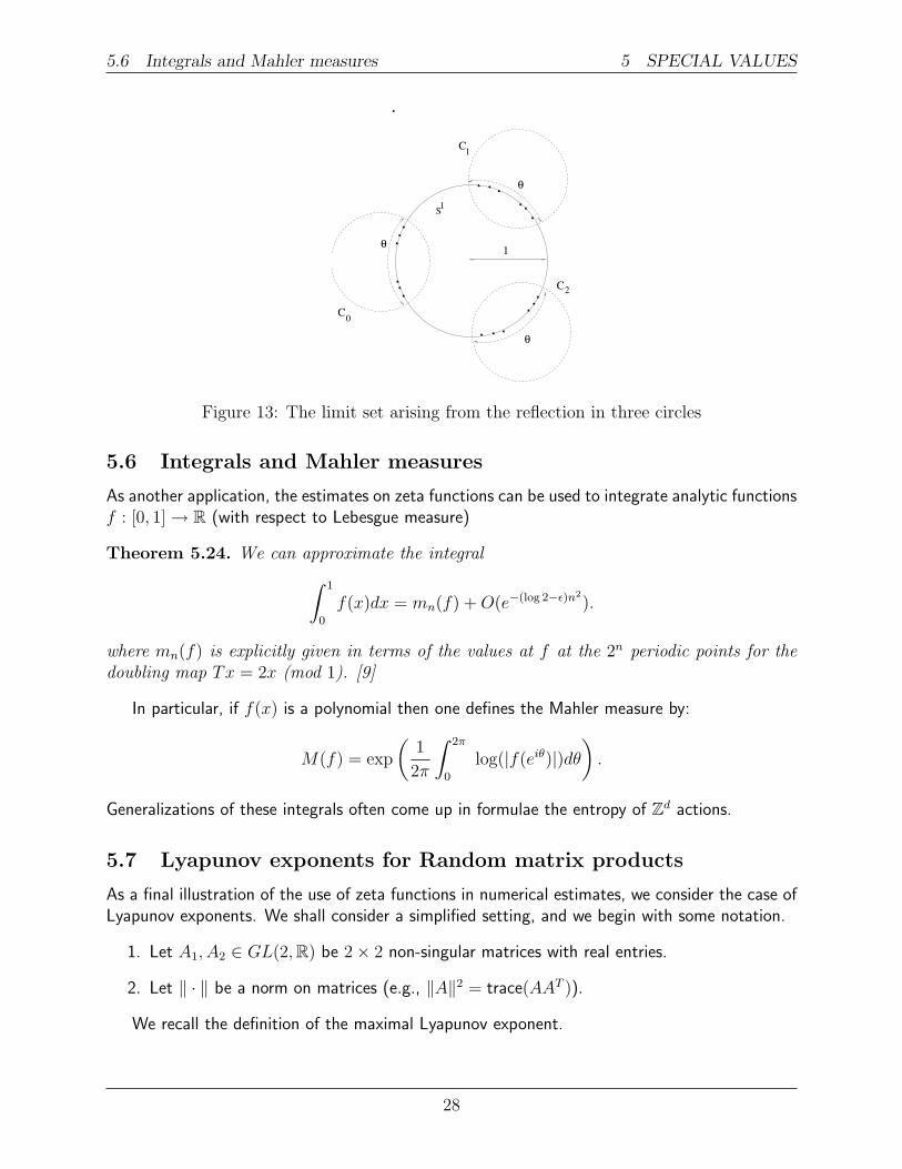
Example 5.21 (McMullen). Consider three circles C0, C1, C2 ⊂ C of equal radius, arrangedsymmetrically around S1, each intersecting S1 orthogonally, and meeting S1 in an arc oflength θ, where 0 < θ < 2π/3 (see Figure 2). Let Λθ ⊂ S1 denote the limit set associated tothe group Γθ of transformations given by reflection in these circles.

For example, with the value θ = π/6 we show that the dimension of the limit set Λπ/6 is

dim(Λπ/6) = 0.18398306124833918694118127344474173288 . . .

which is empirically accurate to the 38 decimal places given.

Remark 5.22. Equivalently, the smallest eigenvalue of the laplacian on H3/Γ is

λ0 = dim(Λπ/6)(2− dim(Λπ/6)) = 0 · 3341163556703682452613106798303932895 · · ·

The main ingredient in the computation of dim(Λ) via the zeros of ζ(z) (or, equalivalently,the determinant) is the following:

Lemma 5.23. Let det(I − zLs) = 1 +∑∞

N=1 dN(s)zN be the power series expansion of thedeterminant of the transfer operator Ls. Then

dN(s) =∑

(n1,...,nm)n1+...+nm=N

(−1)m

m!

m∏l=1

1

nl

∑i∈Fix(nl)

|Dφi(zi)|s

det(I −Dφi(zi)),

where the summation is over all ordered m-tuples of positive integers whose sum is N .

We then choose sN such that ∆N(sN) = 0 where ∆N(s) = 1 +∑∞

N=1 dN(s)zN .

27

5.6 Integrals and Mahler measures 5 SPECIAL VALUES

C

C

C

S

0

1

1

2

1!

!

!

Figure 13: The limit set arising from the reflection in three circles

5.6 Integrals and Mahler measures

As another application, the estimates on zeta functions can be used to integrate analytic functionsf : [0, 1]→ R (with respect to Lebesgue measure)

Theorem 5.24. We can approximate the integral∫ 1

0

f(x)dx = mn(f) +O(e−(log 2−ε)n2

).

where mn(f) is explicitly given in terms of the values at f at the 2n periodic points for thedoubling map Tx = 2x (mod 1). [9]

In particular, if f(x) is a polynomial then one defines the Mahler measure by:

M(f) = exp

(1

2π

∫ 2π

0

log(|f(eiθ)|)dθ).

Generalizations of these integrals often come up in formulae the entropy of Zd actions.

5.7 Lyapunov exponents for Random matrix products

As a final illustration of the use of zeta functions in numerical estimates, we consider the case ofLyapunov exponents. We shall consider a simplified setting, and we begin with some notation.

1. Let A1, A2 ∈ GL(2,R) be 2× 2 non-singular matrices with real entries.

2. Let ‖ · ‖ be a norm on matrices (e.g., ‖A‖2 = trace(AAT )).

We recall the definition of the maximal Lyapunov exponent.

28

6 ZETA FUNCTIONS AND COUNTING

Definition 5.25. The (maximal) Lyapunov Exponent is defined to be

λ := limn→∞

1

2n1

n

∑i1,··· ,in∈{1,2}

log ‖Ai1 · · ·Ain‖︸︷︷︸=:λn

Such Lyapunov exponents play an important role in various setting (e.g., skew product dy-namical systems, hidden Markov processes, etc.). This leads naturally to the following question.

Question 5.26. How do we estimate λ?

We have the following result.

Theorem 5.27. For each n ≥ 1 one can find approximations ξn which converge to λ super-

exponentially, i.e., ∃β > 0 such that |λ− ξn| = O(e−βn

2)

. [17]

For each n ≥ 1, we can consider the finite products of matrices Ai1 · · ·Ain , where i1, · · · , in ∈{1, 2}. The numbers ξn are explicitly defined in terms of the entries and eigenvalues of these 2n

matrices. The number of matrices we need to compute ξn grows exponentially, i.e.,

]{Ai1 · · ·Ain : i1, · · · , in ∈ {1, 2}} = 2n

and so it is particularly significant that the convergence in the theorem is superexponential.

Example 5.28. Let p1 = p2 = 12

and choose

A1 =

(2 11 1

)and A2 =

(3 12 1

)then with n = 9:

λ = 1 · 1433110351029492458432518536555882994025︸︷︷︸=ξn=9

+O(10−40

).

6 Zeta functions and counting

One of the most useful applications of zeta functions is in counting problems.

6.1 Prime Number Theorem

Recall the following classical result proved independently by Hadamard and de Vallee Poussin.

Theorem 6.1 (Prime number theorem). The number π(x) of primes numbers less than xsatisfies

π(x) ∼ x

log xas x→ +∞.

The standard proof uses the Riemann zeta function and two of its basic properties:

29

6.2 The Prime Geodesic Theorem for κ = −1 6 ZETA FUNCTIONS AND COUNTING

1. ζ(s) has a simple pole at s = 1;

2. ζ(s) otherwise has a zero free analytic extension to a neighbourhood of Re(s) = 1.

Thereafter the traditional proofs of the prime number theorem then use either the residure theoremor the Ikehara-Wiener Tauberian theorem.

A knowledge of the Riemann hypothesis would improve the asymptotic in the Prime NumberTheorem to the following:

Conjecture 6.2 (Riemann Hypotheis: alternative formulation).

π(x) =

∫ x

2

1

log udu+O

(x1/2 log x

)This, of course, contains the original Prime Number Theorem since the leading term satisfies∫ x

21

log udu ∼ x

log x. In the absence of the Riemann Conjecture the orginal proof of Hadamard

and de la Vallee Poussin still shows that there were no zeros in a region {s = σ + it : σ >1− C/ log |t| and |t| ≥ 1}. This corresponds to an error term of

π(x) =

∫ x

2

1

log udu+O

(xe−a√

log |x|).

6.2 The Prime Geodesic Theorem for κ = −1

There is a corresponding result for closed geodesics on negatively curved surfaces with curvatureκ = −1, due to Huber.

Theorem 6.3 (Prime geodesic theorem for κ = −1). Let V be a compact surface withκ = −1. The number N(x) of closed geodesics with el(γ) ≤ x less than x satisfies

N(x) ∼ x

log xas x→ +∞.

Equivalently, we have that

Card{γ : l(γ) ≤ T} ∼ eT

Tas T → +∞.

This follows from an analysis of the Selberg Zeta function Z(s). In particular, since a partialanalogue of the Riemann Hypothesis holds in this case, one sees that a partial analogue of theconjectured error term for primes holds:

Theorem 6.4. There exists ε > 0 such that

π(x) =

∫ x

2

1

log udu+O

(x1−ε)

The value of ε > 0 is related to the least distance of the zeros for Z(s) from the lineRe(s) = 1. This is determined by the smallest non-zero eigenvalue of the laplacian. By a resultof Schoen-Wolpert-Yau, this is comparable size to the length of the shortest geodesic dividing thesurface into two pieces. It also has a dynamical analogue, as the rate of mixing of the associatedgeodesic flow.

30

6.3 Prime geodesic theorem for κ < 0 6 ZETA FUNCTIONS AND COUNTING

Figure 14: When κ = −1 then the value ε can be chosen to be comparable to the length l(γ0)of the shortest closed geodesic γ0

6.3 Prime geodesic theorem for κ < 0

We can ask whether these results are still true in the case of manifolds of variable negativecurvature. Indeed, analogues of these results do hold and it is possible to give proofs using zetafunction methods, but in this broader context there is no analogue of the Selberg trace functionapproach and one has to use the transfer operator method (with analytic functions replaced byC1 functions, say).

Let V be a compact surface with negative curvature κ < 0. We can again define a zeta

function by ζV (s) =∏

γ

(1− e−sl(γ)

)−1. The following is easy to show.

Theorem 6.5. The zeta function ζV (s) converges on the half-plane Re(s) > h where h isthe (topological) entropy.

We recall the elegant definition of entropy due to Anthony Manning. Let V be the universalcover of V . Lift the metric from V to V and let BeV (x0, R) be a ball of radius R > 0 about any

fixed reference point x0 ∈ V .

Definition 6.6. We can then write:

h = limR→+∞

1

Rlog(vol(BeV (x0, R)

))For example, if the curvature κ < 0 is constant then h =

√|κ|.

By analogy with the constant curvature case we have the following results on the domain ofthe zeta function.

Theorem 6.7. There exists h > 0 such that:

1. ζV (s) converges for Re(s) > h;

2. ζV (s) has a simple pole at s = h;

3. ζV (s) otherwise has a non-zero analytic extension to a neighbourhood of Re(s) = h

The same basic proof as for the Prime Number Theorem now gives the Prime GeodesicTheorem.

31

6.4 Counting sums of squares 6 ZETA FUNCTIONS AND COUNTING

Theorem 6.8 (Prime geodesic theorem for κ < 0). Let V be a compact surface with κ < 0.The number N(x) of closed geodesics with ehl(γ) ≤ x less than x satisfies

N(x) ∼ x

log xas x→ +∞.

Equivalently, we have that

Card{γ : l(γ) ≤ T} ∼ ehT

hTas T → +∞.

Definition 6.9. There exists h > 0 such that ζV (s) is analytic for Re(s) > h and s = h isa simple pole. (The value h is simply the topological entropy of the flow φ.)

In the case of the zeta function ζV (s) for more general surfaces of variable negative curvaturewe have typically a weaker result for than for surfaces of constant negative curvature.

Theorem 6.10 (after Dolgopyat). The exists ε > 0 such that ζV (s) has an analytic zero-freeextension to Re(s) > h− ε

The biggest difference from the case of constant curvature is that we have no useful estimateon ε > 0. This has the (expected) following consequence.

Corollary 6.11. We can estimate that the number N(x) of closed geodesics γ with l(γ) ≤ xby

N(x) =

∫ ehx

2

1

log udu+O(e(h−ε)x)

[18]

Remark 6.12. Recall that the Teichmuller flow on the moduli space of flat metrics is a gen-eralization of the geodesic flow on the modular surface. Athreya-Bufetov-Eskin-Mirzakhaniproved the asymptotic formula in this case.

6.4 Counting sums of squares

Let us now recall a result from number theory which will also prove to have a geometeric analogue.Recall that there are asymptotic estimates on the natural numbers which are also sums of twosquares 1, 2, 4, 5, 8, · · · , u2 + v2, · · · (where u, v ∈ N) less than x. For example, we can write:

1 = 02 + 12

2 = 12 + 12

4 = 02 + 22

5 = 12 + 22

8 = 22 + 22

...

32

6.4 Counting sums of squares 6 ZETA FUNCTIONS AND COUNTING

Definition 6.13. Let S(x) = Card{u2 + v2 ≤ x} be the number of such sums of squares lessthan x.

Theorem 6.14 (Ramamnujan-Landau). Then

S(x) ∼ x

(log x)12

as x→ +∞

The theorem was originally proved by Landau in 1908, although it was independently statedin Ramanujan’s first famous letter to Hardy from 16 January 1913.

Hadamard (1865-1963) Ramanujan (1887-1920)

There is a very interesting account of this in the excellent book of Hardy: “Ramanujan:Twelve lectures on subjects suggested by his life and work”. The basic idea of Landau’s proof isthat in place of the zeta function, one uses another complex function (generating function) givenby

η(s) =∞∑n=1

bnn−s where bn =

{1 if n = u2 + v2 is a sum of squares

0 if n is not a sum of squares

This converges for Re(s) > 1. But this has an algebraic pole at s = 1:

Lemma 6.15. We can write

η(s) =C√s− 1

+ A(s)

where A(s) is analytic in a neighbourhood of Re(s) ≥ 1.

Using complex analysis one can write

S(x) =1

2π

∫ c+i∞

c−i∞η(s)

xs

sds for c > 1

and the asymptotic formula comes from moving the line of integration to the left. One canactually get more detailed asymptotic formulae.

Theorem 6.16 (Expansion for sums of squares). There exist constants b0, b1, b2 · · · suchthat

S(T ) =T√

log T

(b0 +

b1

log T+

b2

(log T )2+ · · ·

)as T → +∞.

33

6.5 Closed geodesics in homology classes 6 ZETA FUNCTIONS AND COUNTING

6.5 Closed geodesics in homology classes

Philips and Sarnak considered the problem of additionally restricting to geodesics in a givenhomology class. In particular, they gave an asymptotic formulae for the number N0(T ) of suchclosed geodesics on a surface of constant negative curvature whose length is at most T .

Figure 15: We can restrict the counting to those closed geodesics which are, say, null inhomology as shown in the second figure

More precisely, they established the following result.

Theorem 6.17 (Phillips-Sarnak). For a surface of negative curvature κ = −1, and genusg > 1, there exists c0 such that

N0(T ) ∼ c0eT

T g+1as T → +∞

Moreover, there exist constants c0, c1, c2 such that

N(a, T ) =ehT

T g+1

(c0 + c1/T + c2/T

2 + · · ·)

as T → +∞

[16]

Recall that the asymptotic estimate for counting closed geodesics without the homologyrestrictions gave π(T ) ∼ ehT

hT, which is necessarily larger than N0(T ).

The similar form of the asymptotic arises for the same reason, when on defining the appropriatezeta function using only those geodesics null in homology it leads to a singularity of the form(s − h)−1/2. As one would expect the result extends to surfaces of variable negative curvature,using a similar approach to that used for ζV (s) in order to study the corresponding zeta functionin this case.

Theorem 6.18. For a surface of (variable) negative curvature and genus g > 1 there existconstants c0, c1, c2 such that

N0(T ) =ehT

T g+1(c0 + c1/T + c2/T

2 + ...) as T → +∞.

[10], [19]

34

7 CIRCLE PROBLEM

7 Circle Problem

We begin with another famous result in number theory. We can consider estimates on the numberN(r) of pairs (n,m) ∈ Z2 such that m2 + n2 ≤ r2. It is easy to see that N(r) ∼ πr2. In fact,there is a better estimate due to Gauss.

Lemma 7.1 (Gauss). N(r) = πr2 +O(r)

The following remains an open problem.

Conjecture 7.2 (Circle problem). For each ε > 0 we have that N(r) = πr2 +O(r1/2+ε)

In the case of the analogue of the circle problem for spaces of negative curvature it is aproblem to even find the main term in the corresponding asymptotic.

Question 7.3. What happens if we replace R2 by the Poincare disk D2, and we replace Z2

by a discrete (Fuchsian) group of isometries?

We address this question in the next subsection.

7.1 Hyperbolic Circle Problem

Let D2 = {z ∈ C : |z| < 1} be the unit disk with the Poincare metric

ds2 =dx2 + dy2

(1− (x2 + y2))2.

of constant curvature κ = −1. This is equivalent to the Poincare upper half plane H2, but thismodel has the advantage that the circle counting pictures look more natural.

Figure 16: This famous Escher picture represents the hyperbolic disk

Consider the action g : D2 → D2 defined by g(z) = az+bbz+a

for g lying in a discrete group

Γ <

{(a b

b a

): a, b ∈ C, |a|2 − |b|2 = 1

}35

7.1 Hyperbolic Circle Problem 7 CIRCLE PROBLEM

Let us assume that Γ is cocompact, i.e., the quotient D2/Γ is compact.Consider the orbit Γ0 orbit of the fixed reference point 0 ∈ D2. The following is the analogue

of the circle problem for negative curvature.

Question 7.4. What are the asymptotic estimates for the counting function N(T ) = Card{g ∈Γ : d(0, g0) ≤ T} as T → +∞?

T

0

Figure 17: We want to count the points in the orbit Γ0 of 0 which are at a distance at mostT from 0.

More generally, we can consider the orbit of a fixed reference point x ∈ D2. We want to findasymptotic estimates for the counting function

N(T ) = Card{g ∈ Γ : d(x, gx) ≤ T}

Assume that Γ is cocompact, i.e., the quotient surface V = D2/Γ is compact.

Theorem 7.5. There exists C > 0. N(R) ∼ CeT as T → +∞.

In fact there is an error term in this case too.

Theorem 7.6. There exists C > 0 and ε > 0. N(R) = CeT +O(e(1−ε)T ) as T → +∞.

The basic method of proof is the same as for counting primes and closed geodesics. In placeof the zeta function one wants to study the Poincare series.

Definition 7.7. We define the Poincare series by

η(s) =∑g∈Γ

e−sd(gx,x)

where s ∈ C. This converges to an analytic function for Re(s) > 1.

The Poincare series can be shown to have the following analyticity properies:

Lemma 7.8. The Poincare series has a meromorphic extension to C with a simple pole ats = 1 and no poles other poles on the line Re(s) = 1.

36

7.2 Schottky groups and the hyperbolic circle problem 7 CIRCLE PROBLEM

The proof of this result is usually based on the Selberg trace formula (and this is wherewe use that Γ is cocompact). In order to show how it leads to a proof of the theorem, letL(T ) = Card{g ∈ Γ : exp(d(x, gx)) ≤ T} for T > 0. We can then write

η(s) =

∫ ∞1

t−sdL(t)

and employ the following standard Tauberian Theorem

Lemma 7.9 (Ikehara-Wiener). If there exists C > 0 such that

ψ(s) =

∫ ∞1

t−sdL(t)− C

s− 1

is analytic in a neighbourhood of Re(s) ≥ h then L(T ) ∼ CT as T → +∞.

Finally, we can deduce from L(T ) ∼ CT that N(T ) ∼ CeT as T → +∞., which completesthe proof.

7.2 Schottky groups and the hyperbolic circle problem

Assume that Γ is a Schottky group. In particular, we require that Γ is a free group, althoughwe shall assume that D2/Γ is non-compact. In this context the hyperbolic analogue of the circlecounting problem takes a slightly different form.

Theorem 7.10. There exists C > 0 and δ > 0 such that

N(T ) := Card{g ∈ Γ : d(0, g0) ≤ T} ∼ CeδT

as T → +∞.

Here 0 < δ < 2 is the Hausdorff dimension of the limit set (i.e., the Euclidean accumulationpoints of the orbit Γ0 on the unit circle). We can briefly sketch the proof in this case.

1st step of proof: We define the Poincare series by

η(s) =∑g∈Γ

e−sd(g0,0).

This converges to an analytic function for Re(s) > δ. Moreover, we can establish the followingresult on the domain of η(s)

Lemma 7.11. The Poincare series has a meromorphic extension to C with:

1. a simple pole at s = δ; and

2. no poles other poles on the line Re(s) = δ.

37

7.3 Apollonian circle packings 7 CIRCLE PROBLEM

When D2/Γ is compact then this result is based on the Selberg trace formula. However, whenΓ is Schottky group a dynamical approach works better, as in step 3 (with a hint of automaticgroup theory, as in step 2)

2nd step of proof: Consider the model case of a Schottky group Γ = 〈a, b〉. In this case, eachg ∈ Γ− {e} can be written g = g1g2 · · · gn, say, where gi ∈ {a, b, a−1, b−1} with gi 6= g−1

i+1.

Definition 7.12. Consider the space of infinite sequences

ΣA = {(xn)∞n=0 : A(xn, xn+1) = 1 for n ≥ 0}, where A =

(1 1 0 11 1 1 00 1 1 11 0 1 1

)and the shift map σ : ΣA → ΣA given by (σx)n = xn+1.

We then have the following way to enumerate the displacements d(g0, 0):

Lemma 7.13. There exists a (Holder) continuous function f : ΣA → R and x′ ∈ ΣA suchthat there is a correspondence between the sequences {d(g0, 0) : g ∈ Γ} and{

n−1∑k=0

f(σky) : σny = x′, n ≥ 0

}.

1st step of proof: Extending the Poincare series comes from the following.

Corollary 7.14. We can write that

η(s) =∞∑n=1

∑σny=x0

exp

(−s

n−1∑k=0

f(σky)

)

To derive the corollary, we define families of transfer operators Ls : C(ΣA)→ C(ΣA), s ∈ C,by

Lsw(x) =∑σy=x

e−sf(y)w(y), where w ∈ C(ΣA)

then we can formally write

η(s) =∞∑n=1

Lns1(x).

Finally, the better spectral properties of the operators Ls on the smaller space of Holder functionsgive the meromorphic extension and the other properties follow by more careful analysis.

4th step of proof: The final step is just by using the Tauberian theorem, by analogy with theprevious counting results.

38

7.3 Apollonian circle packings 7 CIRCLE PROBLEM

Figure 18: Two very different example of Apollonian circle packings. The numbers representthe curvatures of the circles, i.e., the reciprocal of their radii

7.3 Apollonian circle packings

There is an interesting connection between the hyperbolic circle problem and a problem forApollonian circle packings. Consider a circle packing where four circles are arranged so that eachis tangent to the other three.

Assume that the circles have radii r1, r2, r3, r4 and denote their curvatures by ci = 1ri

.

Lemma 7.15 (Descartes). The curvatures satisfy 2(c21 + c2

2 + c23 + c2

4) = (c1 + c2 + c3 + c4)2

Fir the most familiar Apollonian circle packing we can consider the special case c1 = c2 = 0and c3 = c4 = 1.

The curvatures of the circles are 0, 1, 4, 9, 12, · · ·

Question 7.16 (Lagarias et al). How do these numbers grow?

We want to count these curvatures with their multiplicity.

Definition 7.17. Let C(T ) be the number of circles whose curvatures are at most T .

There is the following asymprotic formula.

Theorem 7.18 (Kontorovich-Oh). There exists K > 0 and δ > 0 such that

C(T ) ∼ KT δ as T → +∞

Remark 7.19. For the standard Apollonian circle packing:

39

7.4 variable curvature 7 CIRCLE PROBLEM

1. The value δ = 1 · 30568 · · · is the dimension of the limit set; and

2. The value K = 0 · 0458 · · · can be estimated too

The proof is dynamical and comes from reformulating the problem in terms of a discreteKleinian group acting on three dimensional hyperbolic space. We briefly recall idea of the proof:

Figure 19: The black circles generate the Apollonian circle packing. Reflecting in the compli-mentary red circles generates the Schottky group

• Given a family of tangent circles (in black) leading to a circle packing, we associate a newfamily of tangent circles (red).

• One then defines isometries of three dimensional hyperbolic space H3 by reflecting in theassociated geodesic planes (i.e., hemispheres in upper half-space).

• Let Γ be the Schottky group (for H3) then one can reduce the theorem to a countingproblem for Γ.

Question 7.20. Can these results be generalized to other circle packings?

7.4 variable curvature

Let now assume that V is a surface of variable negative curvature. Let V be the universal coveringspace for V with the lifted metric d. The covering group Γ = π1(V ) acts be isometries on V

and V /Γ. We want to find asymptotic estimates for the counting function

N(T ) = Card{g ∈ Γ : d(x, gx) ≤ T}

Let h > 0 be the topological entropy.

Theorem 7.21. There exists C > 0. N(R) ∼ CehT as T → +∞.

One might expect the following result to be true:

Conjecture 7.22. There exists C > 0 and ε > 0. N(T ) = CeT +O(e(1−ε)T ) as T → +∞.

40

8 THE EXTENSION OF ζV (S) FOR κ < 0

The basic method of proof is the same as for counting primes and closed geodesics. In placeof the zeta function one wants to study the Poincare series.

Definition 7.23. We define

η(s) =∑g∈Γ

e−sd(gx,x)

This converges to an analytic function for Re(s) > h.

Lemma 7.24. The Poincare series has a meromorphic extension to C with a simple pole ats = 1 and no poles other poles on the line Re(s) = h.

Let M(T ) = Card{g ∈ Γ : exp(hd(x, gx)) ≤ T} then we can write

η(s) =

∫ ∞1

t−sdM(t)

and use the Tauberian Theorem to deduce that M(T ) ∼ CT and thus that N(T ) ∼ CehT asT → +∞.

8 The extension of ζV (s) for κ < 0

Consider a compact surface V of variable curvature κ < 0 and the associated geodesic flowφt : M → M on the unit tangent bundle M = SV . In order to extend the zeta function ζV (s)to all s ∈ C we need to develop different machinery. Motivated by work of Gouezel-Liverani (andBaladi-Tsujii) for Anosov diffeomorphisms, we want to employ the basic philosophy: We want tostudy simple operators on complicated Banach spaces” . More precisely, following Butterley andLiverani:

Definition 8.1. For each s ∈ C let R(s) : C0(M)→ C0(M) be the operator defined by

R(s)w(x) =

∫ ∞0

e−stLtw(x)dt where w ∈ C0(M)

where Ltw(x) = w(φtx) is simply composition with the flow.

We need to replace C0(M) by a “better” Banach space, for which there is less spectrum.Actually, we need a family of complicated Banach spaces. For each k ≥ 1 we can associate aBanach space of distributions Bk such that the restriction R(s) : Bk → Bk has only isolatedeigenvalues for Re(s) > −k.

We then want to use the operator Lt to extend ζV (s). We need to make sense of

“det(I −R(s)) = exp

(∞∑n=1

1

ntr (R(s)n)

)′′for operators R(s) which are not trace class.

Finally, we need to relate ζV (s) to “det(I−R(s))′′, which in fact means we have to do repeatthe analysis all over again for Banach spaces of differential forms as well as functions in order tofix up the identities.

41

9 APPENDIX: SELBERG TRACE FORMULAE

Theorem 8.2 (Giulietti-Liverani-P.). For compact surfaces V with κ < 0:

1. The zeta function ζV (s) has a meromorphic extension to C.

2. For each k ≥ 1, the poles and zeros s = sn for ζV (s) in the region Re(s) > −kcorrespond to 1 being an eigenvalue for R(s).

9 Appendix: Selberg trace formulae

In this survey, we are actually more interested in the dynamical approach to zeta functions, butfor completeness we attempt to sketch the original approach using the Selberg trace formula.

9.1 The Laplacian

Assume that the surface V is compact then there are countably many distinct solutions ∆φi +λiφi = 0 (with ‖φi‖2 = 1 and 0 = λ0 ≤ λ1 ≤ λ2 ≤ · · · → +∞ are real valued, since theoperator is self-adjoint). We define the Heat Kernel on V by

K(x, y, t) =∑n

φn(x)φn(y)e−λnt.

(This has a nice interpretation as the probability of a Brownian Motion path going from x to yin time t > 0.) In particular we can define the trace:

tr(K(·, ·, t)) :=

∫M

K(x, x, t)dν(x) =∑n

e−λnt.

9.2 Homogeneity and the trace

We can consider the Poincare distance between x, y ∈ H2 given by

d(x, y) = cosh−1

(1 +

|x− y|2

2Im(x).Im(y)

).

The heat kernel is homogeneous, i.e., the heat kernel K(·, ·, t) on H2 depends only on the relativedistance d(x, y) apart of x, y ∈ H2. Let us now fix lifts x and y of x and y, respectively, in somefundamental domain F . We can then write

K(x, y.t) =∑γ∈Γ

K(x, γy, t) =∑γ∈Γ

K(d(x, γy), t)

and evaluate the trace

tr(K(·, ·, t)) :=

∫F

K(x, x, t)dν(x) =

∫F

K(d(x, x), t)dν(x) +∑

γ∈Γ−{e}

∫F

K(d(x, γx), t)dν(x).

Lemma 9.1. There is a correspondence between Γ and {kpnk−1 : n ∈ Z, p, k ∈ Γ/Γp} wherep runs through the non-conjugate primitive elements of Γ and g ∈ Γ.

42

9.3 Explicit formulae and Trace formula9 APPENDIX: SELBERG TRACE FORMULAE

Since ν is preserved by translation by elements of the group, we can write

∑γ∈Γ−{e}

∫F

K(d(x, γx), t)dν(x) =∞∑n=1

∑p

∑k∈Γ/Γp

∫F

K(d(k−1x, pnk−1x), t)dν(x)

︸︷︷︸

=R

FpeK(d(x,pnx),t)dν(x)

. (1)

where Fp is a fundamental domain for Γp. Without loss of generality, we can take the fundamentaldomain z = x+ iy where 1 ≤ y ≤ m2 (where l(g) = 2 logm) and the integral can be explicitlyevaluated

l(p)√cosh(l(pn))− 1

∫ ∞cosh l(pn)

K(s)ds√s− cosh l(pn)

. (2)

([12], page 232).

9.3 Explicit formulae and Trace formula

The heat kernel K(x, y, t) on H2 has the following standard explicit form, which we state withoutproof.

Lemma 9.2. One can write

K(x, y, t) = K(d(x, y), t) =

√2

(4πt)3/2e−t/4

∫ ∞d(x,y)

ue−u2/4t√

cosh(u)− cosh(d(x, y))du

and, in particular,

K(0, t) =1

(4π)3/2

∫ ∞0

ue−u2/4t

sinh(u/2)du.

We start with the first term in (1):∫M

K(0, t)dν(x) =ν(M)e−t/4

(4πt)3/2

∫ ∞0

se−s2/4t

sinh(s/2)ds.

The connection with the orginal problem comes via the standard result: The length of a closedgeodesic in the conjugacy class of g is given by l(g) = infx∈H d(xg, x). Moreover, l(gn) = |n|l(g).

Lemma 9.3. There is a bijection between nontrivial conjugacy class and closed geodesics onthe surface. Moreover, tr(g) = 2 cosh(l(γ)).

Furthermore, we can write∑γ∈Γ−{e}

∫M

K(d(x, γx), t)dν(x) =∑[γ]

∫M

K(d(x, γx), t)dν(x)

which allows us to write the rest of the trace explicitly:

43

9.4 Return to the Selberg Zeta function9 APPENDIX: SELBERG TRACE FORMULAE

Corollary 9.4 (McKean). The trace takes the form

ν(M)e−t/4

(4πt)3/2

∫ ∞0

se−s2/4t

sinh(s/2)ds+

e−t/4

(16πt)1/2

∞∑n=1

∑γ

l(γ)

sinh(nl(γ)/2)e(nl(γ))2/4t

where the sum if over γ if over conjugacy classes in Γ.

This is an explicit computation. Using Lemma 9.2 and (2) we have that∫ ∞cosh l(pn)

K(s)ds√s− cosh l(pn)

=

√2e−t/4

(4πt)3/2

∫ ∞cosh l(pn)

∫ ∞s

se−s2/4t√

cosh(u)− cosh(s)duds

which we can immediately evaluate as e−t/4√

8πte−l(p

n)2/4t, and we are done.

9.4 Return to the Selberg Zeta function

The connection to the Selberg zeta function is actually via its logarithmic derivative Z ′(s)/Z(s).

Lemma 9.5. We can write

Z ′(s)

Z(s)= (2s− 1)

∫ ∞0

e−s(s−1)tθ(t)dt

where

θ(t) =∞∑n=0

e−tλn − ν(M)e−t/4

(4πt)3/2

∫ ∞0

se−s2/4t

sinh(s/2)ds

Proof. For s > 1 we can explicitly write

Z ′(s)

Z(s)=∑p

∞∑k=0

l(p)e−(s+k)l(p)

1− e−(s+k)l(p)=∑p

∞∑k=0

l(p)

sinh(l(pn)/2)e−(s−1/2)l(pn)

In particular, we can write

1

2s− 1

Z ′(s)

Z(s)=

∫ ∞0

e−s(s−1)t

(∞∑n=0

e−tλn − 2ν(M)e−t/4

(4πt)3/2

∫ ∞0

se−s2/4t

∞∑n=0

e−(n+1/2)sds

)dt

This can formally be written as

∞∑n=0

(1

s(s− 1)− λn− ν(M)

4π

1

s+ n

)where:

1. The solutions s to s(s− 1) = λn correspond to poles for Z′(s)Z(s)

; and

2. By Gauss-Bonnet ν(M) = 4π(g − 1) and the solutions s = −n correspond to poles forZ′(s)Z(s)

.

44

REFERENCES

10 Final comments

Of course there have been many important contributions to number theory using ergodic theorywhich I have not even touched upon, but which I felt it appropriate to commend to the reader.

1. The first of Khinchin’s pearls was van de Waerden’s theorem (on arithmetic progressions).This, and many deep generalizations, including the recent work of Green and Tao, haveergodic theoretic proofs in the spirit of Furstenberg, etc.

2. Margulis’ proof of the Oppenheim Conjecture (on the values of indefinite quadratic forms)

3. The work of Einseidler, Katok and Lindenstrauss work on the Littlewood conjecture (onsimultaneous diophantine approximations).

4. Benoist-Quint work on orbits of groups on homogeneous spaces.

References

[1] N. Anantharaman and S. Zelditch, Patterson-Sullivan distributions and quantum ergodicity. Ann. HenriPoincar 8 (2007), no. 2, 361–426.

[2] Zeta functions of restrictions of the shift transformation. 1970 Global Analysis (Proc. Sympos. Pure Math.,Vol. XIV, Berkeley, Calif., 1968) pp. 43–49 Amer. Math. Soc., Providence, R.I.

[3] K. Dajani and C. Kraaikamp, Ergodic theory of numbers. Carus Mathematical Monographs, 29. MathematicalAssociation of America, Washington, DC, 2002

[4] L. Flaminio and G. Forni, Invariant distributions and time averages for horocycle flows. Duke Math. J. 119(2003), no. 3, 465–526.

[5] F. Hofbauer and G. Keller, Zeta-functions and transfer-operators for piecewise linear transformations. J.Reine Angew. Math. 352 (1984), 100–113.

[6] D. Hejhal, The Selberg trace formula for PSL(2, R) Vol. I. Lecture Notes in Mathematics, Vol. 548. Springer-Verlag, Berlin-New York, 1976.

[7] K. Ireland, M. Rosen, A classical introduction to modern number theory, Grad. Text. in Math., 84, Springer,Berlin, 1990.

[8] O. Jenkinson and M. Pollicott, Calculating Hausdorff dimensions of Julia sets and Kleinian limit sets. Amer.J. Math. 124 (2002) 495–545.

[9] O. Jenkinson and M. Pollicott, A dynamical approach to accelerating numerical integration with equidis-tributed points. Proc. Steklov Inst. Math. 256 (2007) 275–289

[10] A. Katsuda and T. Sunada, Closed orbits in homology classes. Inst. Hautes tudes Sci. Publ. Math. 71 (1990)5–32

[11] On a ζ function related to the continued fraction transformation. Bull. Soc. Math. France 104 (1976)195–203.

[12] H. McKean, Selberg’s trace formula as applied to a compact Riemann surface. Comm. Pure Appl. Math. 25(1972), 225–246.

45

REFERENCES REFERENCES

[13] J. Milnor and W. Thurston On iterated maps of the interval, Dynamical systems (College Park, MD, 1986–87), 465–563, Lecture Notes in Math., 1342, Springer, Berlin, 1988.

[14] W. Parry and M. Pollicott, Zeta functions and the periodic orbit structure of hyperbolic dynamics. AstrisqueNo. 187-188 (1990) 1-268.

[15] S. J. Patterson, An introduction to the theory of the Riemann zeta-function, Cambridge Studies in AdvancedMathematics, 14. Cambridge University Press, Cambridge, 1988.

[16] R. Phillips and P. Sarnak, Geodesics in homology classes. Duke Math. J. 55 (1987) 287–297.

[17] M. Pollicott, Maximal Lyapunov exponents for random matrix products. Invent. Math. 181 (2010) 209–226.

[18] M. Pollicott and R. Sharp, Exponential error terms for growth functions on negatively curved surfaces. Amer.J. Math. 120 (1998) 1019–1042

[19] M. Pollicott and R. Sharp, Asymptotic expansions for closed orbits in homology classes. Geom. Dedicata 87(2001) 123–160.

[20] D. Ruelle, Generalized zeta-functions for Axiom A basic sets. Bull. Amer. Math. Soc. 82 (1976) 153–156.

[25] P. Sarnak, Class numbers of indefinite binary quadratic forms. J. Number Theory 15 (1982), no. 2, 229–247.

[22] F. Schweiger, Multidimensional continued fractions. Oxford Science Publications. Oxford University Press,Oxford, 2000.

[23] D. Ruelle, Zeta-functions for expanding maps and Anosov flows. Invent. Math. 34 (1976) 231–242

[24] D. Ruelle, Repellers for real analytic maps. Ergodic Theory Dynamical Systems 2 (1982) 99–107

[25] P. Sarnak, Arithmetic quantum chaos. The Schur lectures (1992) (Tel Aviv), 183–236, Israel Math. Conf.Proc., 8, Bar-Ilan Univ., Ramat Gan, 1995.

[26] C. Series, Symbolic dynamics for geodesic flows. Acta Math. 146 (1981) 103–128

[27] S. Smale, Differentiable dynamical systems. Bull. Amer. Math. Soc. 73 1967 747–817.

[28] A. Terras, Harmonic analysis on symmetric spaces and applications. I. Springer-Verlag, New York, 1985.

[29] D. Zagier, Hyperbolic manifolds and special values of Dedekind zeta-functions. Invent. Math. 83 (1986)285–301

46

Dynamical zeta functions - Warwick Insitehomepages.warwick.ac.uk/~masdbl/leiden-lectures.pdf · 1.1...

Documents

Transcript of Dynamical zeta functions - Warwick Insitehomepages.warwick.ac.uk/~masdbl/leiden-lectures.pdf · 1.1...