NBER WORKING PAPER SERIES

VALUATION RISK AND ASSET PRICING

Rui AlbuquerqueMartin S. Eichenbaum

Sergio Rebelo

Working Paper 18617http://www.nber.org/papers/w18617

NATIONAL BUREAU OF ECONOMIC RESEARCH1050 Massachusetts Avenue

Cambridge, MA 02138December 2012

We benefited from the comments and suggestions of Fernando Alvarez, Ravi Bansal, Frederico Belo,Jaroslav Borovika, John Campbell, John Cochrane, Lars Hansen, Anisha Ghosh, Ravi Jaganathan,Tasos Karantounias, Howard Kung, Junghoon Lee, Dmitry Livdan, Jonathan Parker, Alberto Rossi,Costis Skiadas, Ivan Werning, and Amir Yaron. We thank Robert Barro, Emi Nakamura, Jón Steinsson,and José Ursua for sharing their data with us and Benjamin Johannsen for superb research assistance.Albuquerque gratefully acknowledges financial support from the European Union Seventh FrameworkProgramme (FP7/2007-2013) under grant agreement PCOFUND-GA-2009-246542. The views expressedherein are those of the authors and do not necessarily reflect the views of the National Bureau of EconomicResearch. A previous version of this paper was presented under the title "Understanding the EquityPremium Puzzle and the Correlation Puzzle," http://tinyurl.com/akfmvxb.

At least one co-author has disclosed a financial relationship of potential relevance for this research.Further information is available online at http://www.nber.org/papers/w18617.ack

NBER working papers are circulated for discussion and comment purposes. They have not been peer-reviewed or been subject to the review by the NBER Board of Directors that accompanies officialNBER publications.

© 2012 by Rui Albuquerque, Martin S. Eichenbaum, and Sergio Rebelo. All rights reserved. Shortsections of text, not to exceed two paragraphs, may be quoted without explicit permission providedthat full credit, including © notice, is given to the source.

Valuation Risk and Asset PricingRui Albuquerque, Martin S. Eichenbaum, and Sergio RebeloNBER Working Paper No. 18617December 2012, Revised June 2015JEL No. G12

ABSTRACT

Standard representative-agent models fail to account for the weak correlation between stock returnsand measurable fundamentals, such as consumption and output growth. This failing, which underliesvirtually all modern asset-pricing puzzles, arises because these models load all uncertainty onto thesupply side of the economy. We propose a simple theory of asset pricing in which demand shocksplay a central role. These shocks give rise to valuation risk that allows the model to account for keyasset pricing moments, such as the equity premium, the bond term premium, and the weak correlationbetween stock returns and fundamentals.

Rui AlbuquerqueBoston UniversitySchool of Management595 Commonwealth AvenueBoston, MA 02215and Portuguese Catholic Universityralbuque@bu.edu

Martin S. EichenbaumDepartment of EconomicsNorthwestern University2003 Sheridan RoadEvanston, IL 60208and NBEReich@northwestern.edu

Sergio RebeloNorthwestern UniversityKellogg School of ManagementDepartment of FinanceLeverone HallEvanston, IL 60208-2001and NBERs-rebelo@northwestern.edu

1. Introduction

In standard representative-agent asset-pricing models, the expected return to an asset re-

flects the covariance between the asset’s payo§ and the agent’s stochastic discount factor.

An important challenge to these models is that the correlation and covariance between

stock returns and measurable fundamentals, especially consumption growth, is weak at both

short and long horizons. Cochrane and Hansen (1992), Campbell and Cochrane (1999), and

Cochrane (2001) call this phenomenon the correlation puzzle. More recently, Lettau and Lud-

vigson (2011) document this puzzle using di§erent methods. According to their estimates,

the shock that accounts for the vast majority of asset-price fluctuations is uncorrelated with

consumption at virtually all horizons.

The basic disconnect between measurable macroeconomic fundamentals and stock re-

turns underlies virtually all modern asset-pricing puzzles, including the equity-premium

puzzle, Hansen-Singleton (1982)-style rejection of asset-pricing models, violation of Hansen-

Jagannathan (1991) bounds, and Shiller (1981)-style observations about excess stock-price

volatility.

A central finding of modern empirical finance is that variation in asset returns is over-

whelmingly due to variation in discount factors (see Campbell and Ammer (1993) and

Cochrane (2011)). A key question is: how should we model this variation? In classic

asset-pricing models, all uncertainty is loaded onto the supply side of the economy. In Lucas

(1978) tree models, agents are exposed to random endowment shocks, while in production

economies they are exposed to random productivity shocks. Both classes of models abstract

from shocks to the demand for assets. Not surprisingly, it is very di¢cult for these models

to simultaneously resolve the equity premium puzzle and the correlation puzzle.

We propose a simple theory of asset pricing in which demand shocks, arising from sto-

chastic changes in agents’ rate of time preference, play a central role in the determination

of asset prices. These shocks amount to a parsimonious way of modeling the variation in

discount rates stressed by Campbell and Ammer (1993) and Cochrane (2011). Our model

implies that the law of motion for these shocks plays a first-order role in determining the

equilibrium behavior of variables like the price-dividend ratio, equity returns and bond yields.

So, our analysis is disciplined by the fact that the law of motion for time-preference shocks

must be consistent with the time-series properties of these variables.

In our model, the representative agent has recursive preferences of the type considered by

1

Kreps and Porteus (1978), Weil (1989), and Epstein and Zin (1991). When the risk-aversion

coe¢cient is equal to the inverse of the elasticity of intertemporal substitution, recursive

preferences reduce to constant-relative risk aversion (CRRA) preferences. We show that, in

this case, time-preference shocks have negligible e§ects on key asset-pricing moments such

as the equity premium.

We consider two versions of our model. The benchmark model is designed to highlight the

role played by time-preference shocks per se. Here consumption and dividends are modeled

as random walks with conditionally homoscedastic shocks. While this model is very useful

for expositional purposes, it su§ers from some clear empirical shortcomings, e.g. the equity

premium is constant. For this reason, we consider an extended version of the model in which

the shocks to the consumption and dividend process are conditionally heteroskedastic. We

find that adding these features improves the performance of the model.1

We estimate our model using a Generalized Method of Moments (GMM) strategy, im-

plemented with annual data for the period 1929 to 2011. We assume that agents make

decisions on a monthly basis. We then deduce the model’s implications for annual data, i.e.

we explicitly deal with the temporal aggregation problem.2

It turns out that, for a large set of parameter values, our model implies that the GMM esti-

mators su§er from substantial small-sample bias. This bias is particularly large for moments

characterizing the predictability of excess returns and the decomposition of the variance of

the price-dividend ratio proposed by Cochrane (1992). In light of this fact, we modify the

GMM procedure to focus on the plim of the model-implied small-sample moments rather

than the plim of the moments themselves. This modification makes an important di§erence

in assessing the model’s empirical performance.

We show that time-preference shocks help explain the equity premium as long as the risk-

aversion coe¢cient and the elasticity of intertemporal substitution are either both greater

than one or both smaller than one. This condition is satisfied in the estimated benchmark

and extended models.

Allowing for sampling uncertainty, our model accounts for the equity premium and the

volatility of stock and bond returns, even though the estimated degree of agents’ risk aversion

is very moderate (roughly 1.5). Critically, the extended model also accounts for the mean,

1These results parallel the findings of Bansal and Yaron (2004) who show that allowing for conditionalheteroskedasticity improves the performance of long-run risk models.

2Bansal, Kiku, and Yaron (2013) pursue a similar strategy in estimating a long-run risk model. Theyestimate the frequency with which agents make decisions and find that it is roughly equal to one month.

2

variance and persistence of the price-dividend ratio and the risk-free rate. In addition, it

accounts for the correlation between stock returns and fundamentals such as consumption,

output, and dividend growth at short, medium and long horizons. The model also accounts

for the observed predictability of excess returns by lagged price-dividend ratios.

We define valuation risk as the part of the excess return to an asset that is due to the

volatility of the time-preference shock. According to our estimates, valuation risk is a much

more important determinant of asset returns than conventional risk. We show that valuation

risk is an increasing function of an asset’s maturity. So, a natural test of our model is whether

it can account for bond term premia and the return on stocks relative to long-term bonds.

We pursue this test using stock returns as well as real returns on bonds of di§erent maturity

and argue that the model’s implications are consistent with the data.

An important distinction between our model and leading alternatives lies in the predic-

tions for the slope of the yield curve. With this distinction in mind, we discuss evidence on

the slope of the yield curve obtained using data for the U.S. and the U.K. We then assess the

quantitative implications of di§erent models for the slope of the yield curve. Finally, we show

that the estimated SDF for our model has the properties that Backus and Zin (1994) argue

are necessary to simultaneously account for the slope of the yield curve and the persistence

of bond yields.

There is a literature that models shocks to the demand for assets as arising from time-

preference or taste shocks. For example, Garber and King (1983) and Campbell (1986)

consider these types of shocks in early work on asset pricing. Stockman and Tesar (1995),

Pavlova and Rigobon (2007), and Gabaix and Maggiori (2013) study the role of taste shocks

in explaining asset prices in open economy models. In the macroeconomic literature, Eg-

gertsson and Woodford (2003) and Eggertsson (2004), model changes in savings behavior

as arising from time-preference shocks that make the zero lower bound on nominal interest

rates binding.3 Hall (2014) stresses the importance of variation in discount rates in explain-

ing the cyclical behavior of unemployment. Bai, Rios-Rull and Storesletten (2014) stress the

importance of demand shocks in generating business cycle fluctuations.

Time-preference shocks can also be thought of a simple way of capturing the notion that

fluctuations in market sentiment contribute to the volatility of asset prices, as emphasized

by authors such as in Barberis, Shleifer, and Vishny (1998) and Dumas, Kurshev and Up-

3See also Huo and Rios-Rull (2013), Correia, Farhi, Nicolini, and Teles (2013), and Fernandez-Villaverde,Guerron-Quintana, Kuester, Rubio-Ramírez (2013).

3

pal (2009). Finally, in independent work, contemporaneous with our own, Maurer (2012)

explores the impact of time-preference shocks in a calibrated continuous-time representative

agent model with Du¢e-Epstein (1992) preferences.4

Our paper is organized as follows. In Section 2 we document the correlation puzzle using

U.S. data for the period 1929 to 2011 and the period 1871 to 2006. In Section 3, we present

our benchmark and extended models. We discuss our estimation strategy in Section 4. In

Section 5, we present our empirical results. In Section 6, we study the empirical implications

of the model for bond term premia, as well as the return on stocks relative to long-term

bonds. Section 7 concludes.

2. The correlation puzzle

In this section we examine the correlation between stock returns and fundamentals as mea-

sured by the growth rate of consumption, output, dividends, and earnings.

2.1. Data sources

We consider two sample periods: 1929 to 2011 and 1871 to 2006. For the first sample, we

obtain nominal stock and bond returns from Kenneth French’s website. We use the measure

of real consumption expenditures and real Gross Domestic Product constructed by Barro and

Ursúa (2011), which we update to 2011 using National Income and Product Accounts data.

We compute per-capita variables using total population (POP).5 We obtain data on real

S&P500 earnings and dividends from Robert Shiller’s website. We use data from Ibbotson

and Associates on the nominal return to one-month Treasury bills, the nominal yield on

intermediate-term government bonds (with approximate maturity of five years), and the

4Normandin and St-Amour (1998) study the impact of preference shocks in a model similar to ours.Unfortunately, their analysis does not take into account the fact that covariances between asset returns,consumption growth, and preferences shocks depend on the parameters governing preferences and technology.As a result, their empirical estimates imply that preference shocks reduce the equity premium. In addition,they argue that they can explain the equity premium with separable preferences and preference shocks. Thisclaim contradicts the results in Campbell (1986) and the theorem in our Appendix B.

5This series is not subject to a very important source of measurement error that a§ects another commonly-used population measure, civilian noninstitutional population (CNP16OV). Every ten years, the CNP16OVseries is adjusted using information from the decennial census. This adjustment produces large discontinuitiesin the CNP16OV series. The average annual growth rates implied by the two series are reasonably similar:1.2 for POP and 1.4 for CNP16OV for the period 1952-2012. But the growth rate of CNP16OV is threetimes more volatile than the growth rate of POP. Part of this high volatility in the growth rate of CNP16OVis induced by large positive and negative spikes that generally occur in January. For example, in January2000, 2004, 2008, and 2012 the annualized percentage growth rates of CNP16OV are 14.8, −1.9, −2.8, and8.4, respectively. The corresponding annualized percentage growth rates for POP are 1.1, 0.8, 0.9, and 0.7.

4

nominal yield on long-term government bonds (with approximate maturity of twenty years).

We convert nominal returns and yields to real returns and yields using the rate of inflation

as measured by the consumer price index. We also use inflation-adjusted U.K. government

bonds (index-linked gilts) with maturities 2.5, 5, 10, 15, and 25 years.

For the second sample, we use data on real stock and bond returns from Nakamura,

Steinsson, Barro, and Ursúa (2013). We use the same data sources for consumption, expen-

ditures, dividends and earnings as in the first sample.

In our estimation, we use two measures of real bond returns. Our primary measure

is the ex-ante real return on nominal, one-year, five-year and twenty-year Treasury bonds

taken from Luo (2014). Luo (2014) constructs alternative models of expected inflation for

one, five and twenty-year horizons. He argues that the random walk model does a better

job at forecasting one-year inflation than more sophisticated models like time-varying VAR

methods of the sort considered by Primiceri (2005). It also does better than Bayesian vector

autoregressions embodying Minnesota priors. However, he argues that the latter does best

at forecasting inflation at the five- and twenty-year horizons.

We also report results for a second measure of real bond returns: the realized real return

on nominal one-year, five-year and twenty-year Treasury bonds. The one-year rate is the

measure of the risk-free rate used in Mehra and Prescott (1985) and the associated literature.

We compute dynamic correlations between stock returns and consumption growth for the

G7 and OECD countries. The data on annual real stock returns for the G7 and the OECD

countries are from Global Financial Statistics. The data on real per capita personal consumer

expenditures and real per capita Gross Domestic Product (GDP) for these countries comes

from Barro and Ursúa (2008) and was updated by these authors until 2009. The countries

(beginning of sample period) included in our data set are: Australia (1901), Austria (1947),

Belgium (1947), Canada (1900), Chile (1900), Denmark (1900), Finland (1923), France

(1942), Germany (1851), Greece (1953), Italy (1900), Japan (1894), Korea (1963), Mexico

(1902), Netherlands (1947), New Zealand (1947), Norway (1915), Spain (1941), Sweden

(1900), Switzerland (1900), United Kingdom (1830), and United States (1869).

2.2. Empirical results

Table 1, panel A presents results for the sample period 1929 to 2011. We report correlations

at the one-, five- and ten-year horizons. The five- and ten-year horizon correlations are

computed using five- and ten-year overlapping observations, respectively. We report Newey-

5

West (1987) heteroskedasticity-consistent standard errors computed with ten lags.

There are three key features of Table 1, panel A. First, consistent with Cochrane and

Hansen (1992) and Campbell and Cochrane (1999), the growth rates of consumption and

output are uncorrelated with stock returns at all the horizons that we consider. Second, the

correlation between stock returns and dividend growth is similar to that of consumption and

output growth at the one-year horizon. However, the correlation between stock returns and

dividend growth is substantially higher at the five and ten-year horizons than the analogue

correlations involving consumption and output growth. Third, the pattern of correlations

between stock returns and dividend growth is similar to the analogue correlations involving

earnings growth.

Table 1, panel B reports results for the longer sample period (1871-2006). The one-

year correlation between stock returns and the growth rates of consumption and output

are very similar to those obtained for the shorter sample. There is evidence in this sample

of a stronger correlation between stock returns and the growth rates of consumption and

output at a five-year horizon. But, at the ten-year horizon the correlations are, once again,

statistically insignificant. The results for dividends and earnings are very similar across the

two subsamples.

Table 2 assesses the robustness of our results for the correlation between stock returns

and consumption using three di§erent measures of consumption for the period 1929 to 2011,

obtained from the National Product and Income Accounts. With one exception, the corre-

lations in this table are statistically insignificant. The exception is the five-year correlation

between stock returns and the growth rate of nondurables and services which is marginally

significant.

Table 3 reports the correlation between stock returns and the growth rate of consumption

and output for the G7, and the OECD. We report correlations at the one-, five- and ten-

year horizons. We compute correlations for the G7 and the OECD countries pooling data

across all countries. This procedure implies that countries with longer time series receive

more weight in the calculations. Again, there is also a relatively weak correlation between

consumption and output growth and stock returns at all the horizons we consider.

We have focused on correlations because we find them easy to interpret. One might

be concerned that a di§erent picture emerges from the pattern of covariances between stock

returns and fundamentals. It does not. For example, using quarterly U.S. data for the period

6

1959 to 2000, Parker (2001) argues that one would require a risk aversion coe¢cient of 379

to account for the equity premium given his estimate of the covariance between consumption

growth and stock returns.6

We conclude this subsection by considering the dynamic correlations between consump-

tion growth and stock returns. Authors like Parker (2001), Campbell (2003), and Jaganathan

and Wang (2007) find that in the U.S. post-war quarterly data, stock returns are correlated

with future consumption growth.7 Figure 1 reports the correlation between returns at time

t and consumption growth at time t+ τ , where τ ranges from −10 years to +10 years. The

dotted lines are the limits of the 95 percent confidence interval. The figure also reports the

analogue correlations involving output growth. Three key features are worth noting. First,

for the U.S. and Canada there does appear to be a significant correlation between returns

at time t and both consumption and output growth at time t + 1. Second, this result is

not robust across the other G7 countries. Third, there is no other value of τ for which the

correlation is significant for any of the countries. So, we infer that, even taking dynamic cor-

relations into account, there is a weak correlation between stock returns and fundamentals,

as measured by consumption and output growth. Nevertheless, because we estimate our

structural model using U.S. data, we assess its ability to be consistent with the correlations

between stock returns at t and consumption growth at t+ 1.

Viewed overall, the results in this section serve as our motivation for introducing shocks

to the demand for assets. Classic representative-agent models load all uncertainty onto the

supply-side of the economy. As a result, they have di¢culty in simultaneously accounting

for the equity premium and the correlation puzzle.8 This di¢culty is shared by the habit-

formation model proposed by Campbell and Cochrane (1999) and the long-run risk models

proposed by Bansal and Yaron (2004) and Bansal, Kiku, and Yaron (2012). Rare-disaster

models of the type proposed by Rietz (1988) and Barro (2006) also share this di¢culty

because all shocks, disaster or not, are to the supply side of the model. A model with a time-

varying disaster probability, of the type considered by Wachter (2012) and Gourio (2012),

6Parker (2001) finds that there is a larger covariance between current stock returns and the cumulativegrowth rate of consumption over the next 12 quarters. He shows that using this covariance measure, onewould require a risk aversion coe¢cient of 38 to rationalize the equity premium (see also Grossman, Melinoand Shiller (1987)).

7In related work, Backus, Routledge, and Zin (2010) show that equity returns is a leading indicator ofthe business-cycle components of consumption and output growth.

8Lynch (1996) and Gârleanu, Kogan, and Panageas (2012) provide interesting analyses of overlapping-generations models which generate an equity premium, even though the correlation between consumptiongrowth and equity returns is low.

7

might be able to rationalize the low correlation between consumption and stock returns

as a small-sample phenomenon. The reason is that changes in the probability of disasters

induce movements in stock returns without corresponding movements in actual consumption

growth. This force lowers the correlation between stock returns and consumption in a sample

where rare disasters are under represented. This explanation might account for the post-war

correlations. But we are more skeptical that it accounts for the results in Table 1, panel B,

which are based on the longer sample period, 1871 to 2006, which includes disasters such as

the Great Depression and two World Wars.

Below, we focus on demand shocks as the source of the low correlation between stock

returns and fundamentals, rather than the alternatives just mentioned. We model these

demand shocks in the simplest possible way by introducing shocks to the time preference of

the representative agent. Consistent with the references in the introduction, these shocks can

be thought of as capturing changes in agents’ attitudes towards savings or, more generally,

investor sentiment.

3. The model

In this section, we study the properties of a representative-agent endowment economy modi-

fied to allow for time-preference shocks. The representative agent has the constant-elasticity

version of Kreps-Porteus (1978) preferences used by Epstein and Zin (1991) and Weil (1989).

The life-time utility of the representative agent is a function of current utility and the cer-

tainty equivalent of future utility, U∗t+1:

Ut = maxCt

hλtC

1−1/ t + δ

"U∗t+1

#1−1/ i1/(1−1/ ), (3.1)

where Ct denotes consumption at time t and δ is a positive scalar. The certainty equivalent

of future utility is the sure value of t+ 1 lifetime utility, U∗t+1 such that:

"U∗t+1

#1−γ= Et

"U1−γt+1

#.

The parameters and γ represent the elasticity of intertemporal substitution and the coef-

ficient of relative risk aversion, respectively. The ratio λt+1/λt determines how agents trade

o§ current versus future utility. We assume that this ratio is known at time t.9 We refer to9We obtain similar results with a version of the model in which the utility function takes the form:

Ut =hC1−1/ t + λtδ

"U∗t+1

#1−1/ i1/(1−1/ ). The assumption that the agents knows λt+1 at time t is made

to simplify the algebra and is not necessary for any of the key results.

8

λt+1/λt as the time-preference shock. Propositions 6.9 and 6.18 in Skiadas (2009) provide a

set of axioms that applies to recursive utility functions with preference shocks.10

3.1. The benchmark model

To highlight the role of time-preference shocks, we begin with a very simple stochastic process

for consumption:

log(Ct+1/Ct) = µ+ σc"ct+1. (3.2)

Here, µ and σc are non-negative scalars and "ct+1 follows an i.i.d. standard-normal distribu-

tion.

As in Campbell and Cochrane (1999), we allow dividends, Dt, to di§er from consumption.

In particular, we assume that:

log(Dt+1/Dt) = µ+ πdc"ct+1 + σd"

dt+1. (3.3)

Here, "dt+1 is an i.i.d. standard-normal random variable that is uncorrelated with "ct+1. To

simplify, we assume that the average growth rate of dividends and consumption is the same

(µ). The parameter σd ≥ 0 controls the volatility of dividends. The parameter πdc controls

the correlation between consumption and dividend shocks.11

The variable Λt+1 = log(λt+1/λt) determines how agents trade o§ current versus future

utility. This ratio is known at time t. We refer to Λt+1 as the time-preference shock. This

shock evolves according to:

Λt+1 = ρΛΛt + σΛ"Λt , (3.4)

where, "Λt is an i.i.d. standard-normal random variable. In the spirit of the original Lucas

(1978) model, we assume, for now, that "Λt is uncorrelated with "ct and "

dt . We relax this

assumption in Subsection 3.4.

The CRRA case In Appendix A we solve this model analytically for the case in which

γ = 1/ . Here preferences reduce to the CRRA form:

Vt = Et

1X

i=0

δiλt+iC1−γt+i , (3.5)

10Skiadas (2009) derives a parametric SDF that satisfies the axioms in proposition 6.9 and 6.18 (see hisequation 6.35). This SDF can be modified to obtain a generalized Epstein and Zin (1989) parametric utilityfunction with stochastic risk aversion, intertemporal substitution, and time-preference shocks. We thankSoohun Kim and Ravi Jagannathan for pointing this result out to us.11The stochastic process described by equations (3.2) and (3.3) implies that log(Dt+1/Ct+1) follows a

random walk with no drift. This implication is consistent with our data.

9

with Vt = U1−γt .

We denote the risk-free rate and the rate of return on a claim on consumption by Rf,t+1,

and Rc,t+1, respectively. The unconditional risk-free rate depends on the persistence and

volatility of time-preference shocks:

E (Rf,t+1) = exp

&σ2Λ/2

1− ρ2Λ

'δ−1 exp(γµ− γ2σ2c/2).

The unconditional equity premium implied by this model is proportional to the risk-free

rate:

E (Rc,t+1 −Rf,t+1) = E (Rf,t+1)(exp

"γσ2c#− 1). (3.6)

Both the average risk-free rate and the volatility of consumption are small in the data.

Moreover, the constant of proportionality in equation (3.6), exp (γσ2c) − 1, is independent

of σ2Λ. So, time-preference shocks do not help to resolve the equity premium puzzle when

preferences are of the CRRA form.

3.2. Solving the benchmark model

We define the return to the stock market as the return to a claim on the dividend process.

The realized gross stock-market return is given by:

Rd,t+1 =Pd,t+1 +Dt+1

Pd,t, (3.7)

where Pd,t denotes the ex-dividend stock price.

It is useful to define the realized gross return to a claim on the endowment process:

Rc,t+1 =Pc,t+1 + Ct+1

Pc,t. (3.8)

Here, Pc,t denotes the price of an asset that pays a dividend equal to aggregate consump-

tion. We use the following notation to define the logarithm of returns on the dividend and

consumption claims, the logarithm of the price-dividend ratio, and the logarithm of the

price-consumption ratio:

rd,t+1 = log(Rd,t+1),

rc,t+1 = log(Rc,t+1),

zdt = log(Pd,t/Dt),

zct = log(Pc,t/Ct).

10

In Appendix B we show that the logarithm of the stochastic discount factor (SDF) implied

by the utility function defined in equation (3.1) is given by:

mt+1 = θ log (δ) + θΛt+1 −θ

∆ct+1 + (θ − 1) rc,t+1, (3.9)

where θ is defined as:

θ =1− γ

1− 1/ . (3.10)

When γ = 1/ , the case of CRRA preferences, the value of θ is equal to one and the

stochastic discount factor is independent of rc,t+1.

We solve the model using the approximation proposed by Campbell and Shiller (1988),

which involves linearizing the expressions for rc,t+1 and rd,t+1 and exploiting the properties

of the log-normal distribution.12

Using a log-linear Taylor expansion we obtain:

rd,t+1 = κd0 + κd1zdt+1 − zdt +∆dt+1, (3.11)

rc,t+1 = κc0 + κc1zct+1 − zct +∆ct+1, (3.12)

where ∆ct+1 ≡ log (Ct+1/Ct) and ∆dt+1 ≡ log (Dt+1/Dt). The constants κc0, κc1, κd0, and

κd1 are given by:

κd0 = log [1 + exp(zd)]− κd1zd,

κc0 = log [1 + exp(zc)]− κc1zc,

κd1 =exp(zd)

1 + exp(zd), κc1 =

exp(zc)

1 + exp(zc),

where zd and zc are the unconditional mean values of zdt and zct.

The Euler equations associated with a claim to the stock market and a consumption

claim can be written as:

Et [exp (mt+1 + rd,t+1)] = 1, (3.13)

Et [exp (mt+1 + rc,t+1)] = 1. (3.14)

We solve the model using the method of undetermined coe¢cients. First, we replace

mt+1, rc,t+1 and rd,t+1 in equations (3.13) and (3.14), using expressions (3.11), (3.12) and

12See Hansen, Heaton, and Li (2008) for an alternative solution procedure.

11

(3.9). Second, we guess and verify that the equilibrium solutions for zdt and zct take the

form:

zdt = Ad0 + Ad1Λt+1, (3.15)

zct = Ac0 + Ac1Λt+1. (3.16)

This solution has the property that price-dividend ratios are constant, absent movements

in Λt+1. This property results from our assumption that the logarithm of consumption and

dividends follow random-walk processes. We compute Ad0, Ad1, Ac0, and Ac1 using the

method of undetermined coe¢cients.

The equilibrium solution has the property that Ad1, Ac1 > 0. We show in Appendix B

that the conditional expected return to equity is given by:

Et (rd,t+1) = − log (δ)− Λt+1 + µ/ (3.17)

+

*(1− θ)

θ(1− γ)2 − γ2

+σ2c/2 + πdc (2γσc − πdc) /2− σ2d/2

+,(1− θ) (κc1Ac1) [2 (κd1Ad1)− (κc1Ac1)]− (κd1Ad1)

2-σ2Λ/2.

Recall that κc1 and κd1 are non-linear functions of the parameters of the model.

Using the Euler equation for the risk-free rate, rf,t+1,

Et [exp (mt+1 + rf,t+1)] = 1,

we obtain:

rf,t+1 = − log (δ)− Λt+1 + µ/ − (1− θ) (κc1Ac1)2 σ2Λ/2 (3.18)

+

*(1− θ)

θ(1− γ)2 − γ2

+σ2c/2.

Equations (3.17) and (3.18) imply that the risk-free rate and the conditional expectation

of the return to equity are decreasing functions of Λt+1. When Λt+1 rises, agents value the

future more relative to the present, so they want to save more. Since risk-free bonds are

in zero net supply and the number of stock shares is constant, aggregate savings cannot

increase. So, in equilibrium, returns on bonds and equity must fall to induce agents to save

less.

The approximate response of asset prices to shocks, emphasized by Borovicka, Hansen,

Hendricks, and Scheinkman (2011) and Borovicka and Hansen (2011), can be directly inferred

12

from equations (3.17) and (3.18). The response of the return to stocks and the risk-free rate

to a time-preference shock corresponds to that of an AR(1) with serial correlation ρΛ.

Using equations (3.17) and (3.18) we can write the conditional equity premium as:

Et (rd,t+1)− rf,t+1 = πdc (2γσc − πdc) /2− σ2d/2 (3.19)

+κd1Ad1 [2 (1− θ)Ac1κc1 − κd1Ad1]σ2Λ/2.

We define the compensation for valuation risk as the part of the one-period expected

excess return to an asset that is due to the volatility of the time preference shock, σ2Λ. We

refer to the part of the one-period expected excess return that is due to the volatility of

consumption and dividends as the compensation for conventional risk.

The component of the equity premium that is due to valuation risk, vd, is given by the

last term in equation (3.19). Since the constants Ac1, Ad1, κc1, and κd1 are all positive, θ < 1

is a necessary condition for valuation risk to help explain the equity premium (recall that θ

is defined in equation (3.10)).13

The intuition for why valuation risk helps account for the equity premium is as follows.

Consider an investor who buys the stock at time t. At some later time, say t + τ , τ > 0,

the investor may get a preference shock, say a decrease in Λt+τ+1, and want to increase

consumption. Since all consumers are identical, they all want to sell the stock at the same

time, so the price of equity falls. Bond prices also fall because consumers try to reduce their

holdings of the risk-free asset to raise their consumption in the current period. Since stocks

are infinitely-lived compared to the one-period risk-free bond, they are more exposed to this

source of risk. So, valuation risk, vd, gives rise to an equity premium. In the CRRA case

(θ = 1) the e§ect of valuation risk on the equity premium is generally small (see equation

3.6)).

It is interesting to highlight the di§erences between time-preference shocks and conven-

tional sources of uncertainty, which pertain to the supply-side of the economy. Suppose that

there is no risk associated with the physical payo§ of assets such as stocks. In this case,

standard asset pricing models would imply that the equity premium is zero. In our model,

there is a positive equity premium that results from the di§erential exposure of bonds and

13As discussed in Epstein et al (2014), the condition θ < 1 also plays a crucial role in generating a highequity premium in long-run risk models. Because long-run risks are resolved in the distant future, they aremore heavily penalized than current risks. For this reason, long-run risk models can generate a large equitypremium even when shocks to current consumption are small.

13

stocks to valuation risk. Agents are uncertain about how much they will value future divi-

dend payments. Since Λt+1 is known at time t, this valuation risk is irrelevant for one-period

bonds. But, it is not irrelevant for stocks, because they have infinite maturity. In general,

the longer the maturity of an asset, the higher is its exposure to time-preference shocks and

the large is the valuation risk.

We conclude by considering the case in which there are supply-side shocks to the economy

but agents are risk neutral (γ = 0). In this case, the component of the equity premium

that is due to valuation risk is always positive as long as < 1. The intuition is as follows:

stocks are long-lived assets whose payo§s can induce unwanted variation in the period utility

of the representative agent, λtC1−1/ t . Even when agents are risk neutral, they must be

compensated for the risk of this unwanted variation.

3.3. Relation to the long-run risk model

In this subsection, we briefly comment on the relation between our model and the long-run-

risk model pioneered by Bansal and Yaron (2004). Both models emphasize low-frequency

shocks that induce large, persistent changes in the agent’s stochastic discount factor.14 To

see this point, it is convenient to re-write the representative agent’s utility function, (3.1),

as:

Ut =hC1−1/ t + δ

"U∗t+1

#1−1/ i1/(1−1/ ), (3.20)

where Ct = λ1/(1−1/ )t Ct. Taking logarithms of this expression we obtain:

log.Ct

/= 1/ (1− 1/ ) log(λt) + log (Ct) .

Bansal and Yaron (2004) introduce a highly persistent component in the process for log(Ct),

which is a source of long-run risk. In contrast, we introduce a highly persistent component

into log(Ct) via our specification of the time-preference shock. From equation (3.9), it is

clear that both specifications can induce large, persistent movements in mt+1. Despite this

similarity, the two models are not observationally equivalent. First, they have di§erent

implications for the correlation between observed consumption growth, log(Ct+1/Ct), and

asset returns. Second, the two models have very di§erent implications for the average return

to long-term bonds, and the term structure of interest rates. We return to these points

when we discuss our empirical results in Section 6. There we present empirical evidence for

14See Dew-Becker (2014) for a version of a long-run risk model in a production economy.

14

the implications of di§erent models for the slope of the yield curve. In addition, we assess

whether the SDFs of the di§erent models have the properties that Backus and Zin (1994)

argue are necessary for explaining the slope of the yield curve and the persistence of bond

yields.

3.4. The extended model

The benchmark model just described is useful to highlight the role of time-preference shocks

in a§ecting asset returns. But its simplicity leads to two important empirical shortcomings.15

First, since consumption is a martingale, the only state variable that is relevant for asset

returns is Λt+1. This property means that all asset returns are highly correlated with each

other and with the price-dividend ratio. Second, and related, the model displays constant

risk premia and so it cannot generate predictability in excess returns.

In this subsection, we address the shortcomings of the benchmark model by allowing for

a richer model of consumption and dividend growth:

log(Ct+1/Ct) = µc + ρc log(Ct/Ct−1) + αc"σ2t+1 − σ2

#+ πcΛ"

Λt+1 + σt"

ct+1, (3.21)

log(Dt+1/Dt) = µd+ρd log(Dt+1/Dt)+αd"σ2t+1 − σ2

#+σdσt"

dt+1+πdΛ"

Λt+1+πdcσt"

ct+1, (3.22)

and

σ2t+1 = σ2 + v"σ2t − σ2

#+ σwwt+1, (3.23)

where "ct+1, "dt+1, "

Λt+1, and wt+1 are mutually uncorrelated standard-normal variables. We

restrict the unconditional average growth rate of consumption and dividends to be the same:

µc1− ρc

=µd

1− ρd.

Relative to the benchmark model, equations (3.21)-(3.23) incorporate three new features.

First, motivated by the data, we allow for serial correlation in the growth rates of consump-

tion and dividends. Second, as in Kandel and Stambaugh (1990) and Bansal and Yaron

(2004), we allow for conditional heteroskedasticity in consumption. This feature generates

time-varying risk premia: when volatility is high the stock is risky, its price is low and its

expected return is high. High volatility leads to higher precautionary savings motive so that

the risk-free rate falls, reinforcing the rise in the risk premium. Third, we allow for a corre-

lation between time-preference shocks and the growth rate of consumption and dividends.15The shortcomings of our benchmark model are shared by other simple models like model I in Bansal

and Yaron (2004), which abstract from conditional heteroskedasticity in consumption and dividends.

15

In a production economy, time-preference shocks would generally induce changes in aggre-

gate consumption. For example, in a simple real-business-cycle model, a persistent increase

in Λt+1 would lead agents to reduce current consumption and raise investment in order to

consume more in the future. Taken literally, an endowment economy specification does not

allow for such a correlation. Importantly, only the innovation to time-preference shocks en-

ters the law of motion for log(Ct+1/Ct) and log(Dt+1/Dt). So, equations (3.21)-(3.23) do not

introduce any element of long-run risk into consumption or dividend growth.

Since the price-dividend ratio and the risk-free rate are driven by a single state variable

in the benchmark model, they have the same degree of persistence. But, according to our

empirical estimates, the price-dividend ratio is more persistent than the risk-free rate. A

straightforward way to address this shortcoming of the benchmark model is to assume that

the time-preference shock is the sum of a persistent shock and an i.i.d. shock:

Λt+1 = xt + σηηt+1, (3.24)

xt+1 = ρΛxt + σΛ"Λt+1.

Here "Λt+1 and ηt+1 are uncorrelated, i.i.d. standard normal shocks. We think of xt as

capturing low-frequency changes in the growth rate of the discount rate. In contrast, ηt+1can be thought of high-frequency changes in investor sentiment that a§ect the demand for

assets (see, for example, Dumas et al. (2009)). If ση = 0 and x1 = Λ1, we obtain the

specification of the time-preference shock used in the benchmark model. Other things equal,

the larger is ση, the lower is the persistence of the time-preference shock.

4. Estimation methodology

We estimate the parameters of our model using the Generalized Method of Moments (GMM).

Our estimator is the parameter vector Φ that minimizes the distance between a vector of

empirical moments, ΨD, and the corresponding model moments, Ψ(Φ). Our estimator, Φ, is

given by:

Φ = argminΦ

[Ψ(Φ)−ΨD]0Ω−1D [Ψ(Φ)−ΨD] .

We found that, for a wide range of parameter values, the model implies that there is small-

sample bias in terms of various moments, especially the predictability of excess returns. We

therefore focus on the plim of the model-implied small-sample moments when constructing

Ψ(Φ), rather than the plim of the moments themselves. For a given parameter vector, Φ, we

16

create 500 synthetic time series, each of length equal to our sample size. For each sample,

we calculate the sample moments of interest. The vector Ψ(Φ) that enters the criterion

function is the median value of the sample moments across the synthetic time series.16 In

addition, we assume that agents make decisions at a monthly frequency and derive the

model’s implications for variables computed at an annual frequency. We estimate ΨD using

a standard two-step e¢cient GMM estimator with a Newey-West (1987) weighting matrix

that has ten lags. The latter matrix corresponds to our estimate of the variance-covariance

matrix of the empirical moments, ΩD.

When estimating the benchmark model, we include the following 19 moments in ΨD: the

mean and standard deviation of consumption growth, the mean and standard deviation of

dividend growth, the contemporaneous correlation between the growth rate of dividends and

the growth rate of consumption, the mean and standard deviation of real stock returns, the

mean, standard deviation and autocorrelation of the price-dividend ratio, the mean, standard

deviation and autocorrelation of the real risk-free rate, the correlation between stock returns

and consumption growth at the one, five and ten-year horizon, the correlation between stock

returns and dividend growth at the one, five and ten-year horizon. We constrain the growth

rate of dividends and consumption to be the same. In practice, when we estimate the

benchmark model we find that the standard deviation of the point estimate of the risk-free

rate across the 500 synthetic time series is very large. So here we report results corresponding

to the case where we constrain the median risk-free rate to exactly match our point estimate.

For the benchmark model, the vector Φ includes nine parameters: γ, the coe¢cient of

relative risk aversion, , the elasticity of intertemporal substitution, δ, the rate of time pref-

erence, σc, the volatility consumption growth shocks, πdc, the parameter that controls the

correlation between consumption and dividend growth shocks, σd, the volatility of dividend

growth shocks, ρΛ, the persistence of time-preference shocks, σΛ, the volatility of the innova-

tion to time-preference shocks, and µ, the mean growth rate of dividends and consumption.

In the extended model, the vector Φ includes nine additional parameters: ρc and ρd,

which control the serial correlation of consumption and dividend growth, αc and αd, which

control the e§ect of volatility on the growth rate of consumption and dividends, respectively,

πcΛ and πdΛ, which control the e§ect of time preference shock innovations on consumption

and dividends, respectively, ν, which governs the persistence of volatility, σw, the volatility

16As the sample size grows, our estimator becomes equivalent to a standard GMM estimator so that theusual asymptotic results for the distribution of the estimator apply.

17

of innovations to volatility, and ση, the volatility of transitory shocks to time preference. In

estimating the extended model, we add to ΨD the following six moments: the first-order

serial correlation of consumption growth, the average yield for 5 and 20-year bonds, and the

slope coe¢cients from the regressions of the excess-equity returns over holding periods of 1,

3 and 5 years on the lagged price-dividend ratio.

5. Empirical results

In the main text, we discuss the results that we obtain estimating the models using the ex-

ante measures of real bond yields. In appendix D, we report the analogue results obtained

estimating the models with ex-post measures of real bond yields.

Table 4 reports our parameter estimates along with standard errors. Several features

are worth noting. First, the coe¢cient of risk aversion is quite low, 1.5 and 2.4, in the

benchmark and extended models, respectively. We estimate this coe¢cient with reasonable

precision. Second, for both models, the intertemporal elasticity of substitution is somewhat

larger than one. Third, for both models, the point estimates satisfy the necessary condition

for valuation risk to be positive, θ < 1. Fourth, the parameter ρΛ that governs the serial

correlation of the growth rate of Λt is estimated to be close to one in both models, 0.991 and

0.992 in the benchmark and extended model, respectively. Fifth, the parameter ν, which

governs the persistence of consumption volatility in the extended model, is also quite high

(0.997). The high degree of persistence in both the time-preference and the volatility shock

are the root cause of the small-sample biases in our estimators.

Table 5 compares the small-sample moments implied by the benchmark and extended

models with the estimated data moments. Recall that in estimating the model parameters

we impose the restriction that the unconditional average growth rate of consumption and

dividends are the same. To assess the robustness of our results to this restriction, we present

two versions of the estimated data moments, with and without the restriction. With one

exception, the constrained and unconstrained data moment estimates are similar, taking

sampling uncertainty into account. The exception is the average growth rate of consumption,

where the constrained and unconstrained estimates are statistically di§erent.

Implications for the equity premium Table 5 shows that both the benchmark and

extended model give rise to a large equity premium, 5.81 and 3.88, respectively. This result

18

holds even though the estimated degree of risk aversion is quite moderate in both models.

In contrast, long-run risk models require a high degree of risk aversion to match the equity

premium.

Recall that in order for valuation risk to contribute to the equity premium, θ must be less

than one. This condition is clearly satisfied by both our models: the estimated value of θ is

−1.6 and −2.6 in the benchmark and extended model, respectively (Table 4). In both cases,

θ is estimated quite accurately. Taking sampling uncertainty into account, the benchmark

model easily accounts for the equity premium, while the extended model does so marginally.

We can easily reject the null hypothesis of θ = 1, which corresponds to the case of constant

relative risk aversion.

The basic intuition for why our model generates a high equity premium despite a low

coe¢cient of relative risk aversion is as follows. From the perspective of the model, stocks

and bonds are di§erent in two ways. First, the model embodies the conventional source of an

equity premium, namely a di§erential covariance of bonds and stocks with the SDF. Since γ

is relatively small, this traditional covariance e§ect is also small. Second, the model embodies

a compensation for valuation risk that is particularly pronounced for stocks because they

they have longer maturities than bonds. Recall that, given our timing assumptions, when

an agent buys a bond at time t, the agent knows the value of Λt+1, so the only source of risk

are movements in the marginal utility of consumption at time t+ 1. In contrast, the time-t

stock price depends on the value of Λt+j, for all j > 1. So, agents are exposed to valuation

risk, a risk that is particularly important because time-preference shocks are very persistent.

Implications for the risk-free rate A problem with some explanations of the equity

premium is that they imply counterfactually high levels of volatility for the risk-free rate

(see e.g. Boldrin, Christiano and Fisher (2001)). Table 5 shows that the volatility of the

risk-free rate and stock market returns implied by our model are similar to the estimated

volatilities in the data.

An empirical shortcoming of the benchmark model is its implication for the persistence

of the risk-free rate. Recall that, according to equation (3.18), the risk-free rate has the same

persistence as the growth rate of the time-preference shock. Table 5 shows that the AR(1)

coe¢cient of the risk-free rate, as measured by the ex-ante real returns to one-year treasury

bills, is only 0.52, with a standard error of 0.07. This estimate is substantially smaller than

the analogue statistic implied by the benchmark model (0.90). The extended model does a

19

much better job at accounting for the persistence of the risk-free rate (0.51). In this model

there are both transitory and persistent shocks to the risk-free rate. The former account for

roughly 44 percent of the variance of Λt.

Implications for the correlation puzzle Table 6 reports the model’s implications for

the correlation of stock returns with consumption and dividend growth.17 Recall that in

the benchmark model consumption and dividends follow a random walk. In addition, the

estimated process for the growth rate of the time-preference shock is close to a random walk.

So, the correlation between stock returns and consumption growth implied by the model is

essentially the same across di§erent horizons. A similar property holds for the correlation

between stock returns and dividend growth.

In the extended model, persistent changes in the variance of the growth rate of consump-

tion and dividends can induce persistent changes in the conditional mean of these variables.

As a result, this model produces correlations between stock returns and fundamentals that

vary across di§erent horizons.

The benchmark model does well at matching the correlation between stock returns and

consumption growth in the data, because this correlation is similar at all horizons. In

contrast, the empirical correlation between stock returns and dividend growth increases with

the time horizon. The estimation procedure chooses to match the long-horizon correlations

and does less well at matching the yearly correlation. This choice is dictated by the fact that

it is harder for the model to produce a low correlation between stock returns and dividend

growth than it is to produce a low correlation between stock returns and consumption growth.

This property reflects the fact that the dividend growth rate enters directly into the equation

for stock returns (see equation (3.11)).

The extended model does better at capturing the fact that the correlations between

equity returns and dividend growth rises with the horizon for two reasons. When volatility

is high, the returns to equity are high. Since αd < 0, the growth rate of dividends is low. As

a result, the one-year correlation between dividend growth and equity returns is negative.

The variance of the shock to the dividend growth rate is mean reverting. So, the e§ect

of a negative value of αd becomes weaker as the horizon extends. The direct association

17The moments reported in this table are slightly di§erent from those reported in Table 1. The reason isthat the moments in the two tables were computed using di§erent samples. In Table 6, we compute a leadedand a lagged correlation, so we lose one observation in the beginning of the sample and another in the endof the sample.

20

between equity returns and dividend growth (see equation (3.11)), which induces a positive

correlation, eventually dominates as the horizon gets longer.

An additional force that allows the extended model to generate a lower short-term cor-

relation between equity returns and dividend growth, is that the estimated value of πdΛ is

negative. The estimation algorithm chooses parameters that allow the model to do rea-

sonably well in matching the one- and five-year correlation, at the cost of doing less well

at matching the ten-year correlation. Presumably, this choice reflects the greater precision

with which the one-year and five-year correlations are estimated relative to the ten-year

correlation. Taking sampling uncertainty into account, the extended model matches the cor-

relation between stock returns and consumption growth at di§erent horizons. Interestingly,

the correlation between stock returns and consumption growth increases with the horizon.

We conclude by highlighting an important di§erence between our model and two leading

alternatives. The first is the external-habit model proposed by Campbell and Cochrane

(1999).18 Working with their parameter values, we find that the correlation between stock

returns and consumption growth are equal to 0.53, 0.69, and 0.62 at the one-, five- and

ten-year horizon, respectively.

The second alternative is the long-run risk model proposed by Bansal, Kiku, and Yaron

(2012). Working with their parameter values, we find that the correlation between stock

returns and consumption growth are equal to 0.34, 0.49, and 0.54 at the one-, five- and

ten-year horizon, respectively. Their model also implies correlations between stock returns

and dividend growth equal to 0.64, 0.90, and 0.93 at the one-, five- and ten-year horizon,

respectively.

Our estimates reported in Table 1 imply that, for both models, the correlations between

fundamentals and returns are counterfactually high. The source of this empirical shortcoming

is that all the uncertainty in the long-run risk model stems from the endowment process.

Implications for the price-dividend ratio In Table 5 we see that both the benchmark

and the extended models match the average price-dividend ratio very well. The benchmark

model somewhat underpredicts the persistence and volatility of the price-dividend ratio. The

extended model does much better at matching those moments. The moments implied by

this model are within two standard errors of their sample counterparts.

18As in Wachter (2005), we consider a version of the model in which equities are a claim to consumption.We thank Jessica Wacher for sharing her program for solving the Campbell-Cochrane model with us.

21

Table 7 presents evidence reproducing the well-known finding that excess returns are

predictable based on lagged price-dividend ratios. We report the results of regressing excess-

equity returns over holding periods of 1, 3 and 5 years on the lagged price-dividend ratio.

The slope coe¢cients are −0.10, −0.27, and −0.42, respectively, while the R-squares are

0.07, 0.14, and 0.26, respectively.

The analogue results for the benchmark model are shown in the top panel of Table 7.

In this model, consumption is a martingale with conditionally homoscedastic innovations.

So, by construction, excess returns are unpredictable in population at a monthly frequency.

Since we aggregate the model to annual frequency, temporal aggregation produces a small

amount of predictability (see column titled “Model (plim)”).

Stambaugh (1999) and Boudoukh et al. (2008) argue that the predictability of excess

returns may be an artifact of small-sample bias and persistence in the price-dividend ratio.

Our results are consistent with this hypothesis. The column labeled “Model (median)”

reports the plim of the small moments implied by our model. The slope coe¢cients for the

1, 5, and 10 year horizons, are −0.05, −0.14 and −0.21, respectively. In each case, the

median Monte Carlo point estimates are contained within a two-standard deviation band of

the respective data estimates.

Table 7 also presents results for the extended model. Because of conditional heteroskedas-

ticity in consumption, periods of high volatility in consumption growth are periods of high

expected equity returns and low equity prices. So, in principle, the model is able to generate

predictability in population. At our estimated parameter values this predictability is quite

small. But, once we allow for the e§ects of small-sample bias, the extended model does quite

well at accounting for the regression slope coe¢cients. Finally, we note that the benchmark

model understates the regression R-squares. Taking sampling uncertainty into account, the

extended model does better on this dimension.

Cochrane (1992) proposes a decomposition of the variation of the price-dividend ratio

into three components: excess returns, dividend growth, and the risk-free rate.19 While this

decomposition is not additive, authors like Bansal and Yaron (2004) use it to compare the

importance of these three components in the model and data.

In our sample, the point estimate for the percentage of the variation in price—dividend

19The fraction of the volatility of the price-dividend ratio attributed to variable x is given by15X

j=1

Ωjcov(zdt, xt+j)/var(zdt), where Ω = 1/(1 + E(Rd,t+1)). See Cochrane (1992) for details.

22

ratio due to excess return fluctuations is 102.2 percent, with a standard error of 30 percent.

Dividend growth accounts for −14.5 with a standard error of 13 percent. Finally, the risk-

free rate accounts for −20.4 percent with a standard error of 14.8 percent. These results are

similar to those in Cochrane (1992) and Bansal and Yaron (2004).

Based on the small-sample moments implied by the benchmark model, the fraction of

the variance of the price-dividend ratio accounted for by excess returns, dividend growth,

and the risk-free rate is 34.6, −2.8, and 54.2, respectively. So, this model clearly overstates

the importance of the risk-free rate and understates the importance of excess returns in

accounting for the variance of the price-dividend ratio.

The extended model does substantially better than the benchmark model. Based on the

small-sample moments implied by the extended model, the fraction of the variance of the

price-dividend ratio accounted for by excess returns, dividend growth, and the risk-free rate

is 51.2, −38.5, and 5.6, respectively. The fraction attributed to excess returns is just within

two standard errors of the point estimate. The fraction attributed to dividend growth is well

within two standard errors of the point estimate.

It is interesting to contrast these results to those in Bansal and Yaron (2004). Their

model also attributes a large fraction of the variance of the price-dividend ratio to excess

returns. At the same time, their model substantially overstates the role of dividend growth

in accounting for the variance of the price-dividend ratio.

Correlation between the price-dividend ratio and the risk-free rate We now dis-

cuss the implications of our model for the correlation between the price-dividend ratio and

the risk-free rate. Table 5 reports that our estimate of this correlation is 0.27 with a stan-

dard error of 0.11. The benchmark model predicts that this correlation should be sharply

negative (−0.95). The intuition for this result is clear. When there is a shock to the rate of

time preference, agents want to save more, both in the form of bonds and stocks. So, the

price-dividend ratio must rise to clear the equity market and the risk-free rate must fall to

clear the bond market. The extended model does much better along this dimension of the

data (−0.20). Recall that a positive shock to "Λt drives the risk-free rate down. Since πdΛ is

negative, the same shock lowers the growth rate of dividends which causes the price dividend

ratio to fall. So the extended mode embodies a force that generates a positive correlation

between the risk-free rate and the price dividend ratio. This forces helps to substantially

lower the sharp negative correlation between these variables in the benchmark model.

23

It is interesting to compare our model with Bansal, Kiku and Yaron (2012). The long-run

risk shock in that model induces a counterfactually sharp positive correlation: 0.65. The

intuition is straightforward. A shock that induces a persistent change in the growth rate of

dividends causes stock prices to go up since equity now represents a claim to a higher flow of

dividends. Dividends do not change much in the short run, so the price-dividend ratio goes

up. At the same time, the shock causes agents to want to shift away from bond holdings and

into equity. So, the risk-free rate must rise to clear the bond market. Other things equal,

the long-run risk shock induces a positive correlation between the price-dividend ratio and

the risk-free rate. In contrast to our model, the Bansal, Kiku and Yaron (2012) does not

embody any forces that would lead to a negative correlation between the price-dividend ratio

and the risk-free rate. The net result is that their model overstates this correlation.

We are hesitant to use this correlation as a litmus test to choose between our model

and Bansal, Kiku and Yaron’s for two reasons. First, the point estimate of this correlation

is sensitive to sample period selection. The correlation is positive (0.17) before 1983 but

negative (−0.44) after 1983. Second, the sign of this correlation varies substantially across

the G7 countries and is again sensitive to breaking the sample in 1983 (see Table 8).

6. Bond term premia

As we emphasize above, the equity premium in our estimated models results primarily from

the valuation risk premium. Since this valuation premium increases with the maturity of an

asset, a natural way to assess the plausibility of our model is to evaluate its implications for

the slope of the real yield curve.

This section is organized as follows. First, we discuss evidence on the slope of the yield

curve obtained using data for the U.S. and the U.K. Second, we discuss the implications

of di§erent models for the yield curve. Third, we evaluate whether the estimated SDF in

our extended model has the properties that Backus and Zin (1994) argue are necessary to

simultaneously account for the slope of the yield curve and the persistence of bond yields.

Finally, we discuss and evaluate the implications of our model for the long-term equity

premium.

Empirical evidence Table 9 reports the mean and standard deviation of ex-ante real

yields on short-term (one year) Treasury Bills, intermediate-term government bonds (with

24

approximate maturity of five years), and long-term government bonds (with approximate

maturity of twenty years).20 The ex-ante yields on five (twenty) year bonds are computed

as the di§erence between the five (twenty) year nominal yield and the ex-ante five (twenty)

year inflation rate (yields are expressed on an annualized basis), which are taken from Luo

(2014).

A number of features are worth noting. First, consistent with Alvarez and Jermann

(2005), the term structure of real yields is upward sloping. Second, the real yield on long-

term bonds is positive. This result is consistent with Campbell, Shiller and Viceira (2009)

who report that the real yield on long-term TIPS has always been positive and is usually

above two percent.

We use data on inflation-index U.K. gilts to shed further light on the slope of the real yield

curve. Table 10 reports the di§erence between the yield of a bond with 2.5 years maturity

and yields of bonds with 5, 10, 15, and 20 years of maturity. Our benchmark sample period

is 1985 to 2015. In every case, the longer duration bond has, on average, a higher yield than

the bond with duration 2.5 years.21 One might be concerned about the e§ect of the recent

financial crisis on these results. As Table 10 indicates, the qualitative results are una§ected

if we use a sample period from 1985 to 2006.22

Model implications Our model implies that long-term bonds command a positive risk

premium that increases with the maturity of the bond (see Appendix C for details on the

pricing of long-term bonds). The latter property reflects the fact that longer maturity assets

are more exposed to valuation risk. Table 9 shows that, taking sampling uncertainty into

account, the benchmark and extended models are consistent with the observed mean yields,

except that the former model generates slightly larger yields for long-term bonds than in the

data. The table also shows that the estimated models account for the volatility of the yields

on short-, intermediate-, and long-term bonds.

Piazzesi and Schneider (2007) and Beeler and Campbell (2012) argue that the bond term

20The moments reported in this table are slightly di§erent from those reported in Table 5. The reason isthat the moments in the two tables were computed using di§erent samples. In Table 5, we compute a leadedand a lagged correlation, so we lose one observation in the beginning of the sample and another in the endof the sample.21The statistical significance of these average di§erences depend on whether we use zero or 12 lags in

computing Newey-West standard errors.22Evans (1998) and Piazzesi and Schneider (2006) finds that the U.K. real yield curve is downward sloping

for the periods January 1983-November 1995 and December 1995-March 2006. Our results indicate thattheir findings depend on the sample period that they work with.

25

premium and the yield on long-term bonds are useful for discriminating between compet-

ing asset pricing models. For example, they stress that long-run risk models, of the type

pioneered by Bansal and Yaron (2004), imply negative long-term bond yields and a nega-

tive bond term premium. The intuition is as follows: in a long-run risk model agents are

concerned that consumption growth may be dramatically lower in some future state of the

world. Since bonds promise a certain payout in all states of the world, they o§er insurance

against this possibility. The longer the maturity of the bond, the more insurance it o§ers

and the higher is its price. So, the term premium is downward sloping. Indeed, the return

on long-term bonds may be negative. Beeler and Campbell (2012) show that the return on

a 20-year real bond in the Bansal, Kiku and Yaron (2012) model is −0.88.

Standard rare-disaster models also imply a downward sloping term structure for real

bonds and a negative real yield on long-term bonds. See, for example the benchmark model

in Nakamura et al. (2013). According to these authors, these implications can be reversed

by introducing the possibility of default on bonds and assuming that probability of partial

default is increasing in the maturity of the bond.23 So, we cannot rule out the possibility

that other asset-pricing models can account for bond term premia and the rate of return on

long-term bonds. Still, it seems clear that valuation risk is a natural explanation of these

features of the data.

Accounting for the slope of the yield curve and the persistence of bond yields

Backus and Zin (1994) investigate the properties of the log of the SDF that are consistent

with two key features of nominal yields: the yield curve is upward sloping and yields are very

persistent. They estimate various ARMA representations for the log of the SDF using data

on the mean and autocovariance of bond yields.24 Their best statistical fit is an ARMA(2,3).

These properties can be summarized as follows. First, the log of the SDF must have negative

serial correlation to account for the positive slope of the nominal yield curve. Second, the

log of the SDF must be close to i.i.d. but still have a small predictable component.25 The

log of the real SDF in both our benchmark and extended model satisfy these two properties.

For an ARMA(2,3), these properties are most easily seen in the impulse response function

23Nakamura et al (2013) consider a version of their model in which the probability of partial default ona perpetuity is 84 percent, while the probability of partial default on short-term bonds is 40 percent. Thismodel generates a positive term premium and a positive real return on long-term bonds.24Bansal and Viswanathan (1993) follow a similar approach but use a semi-nonparametric approximation

to the SDF.25See Ljungqvist and Sargent ( 2000) for a detailed exposition of these two properties.

26

of the extended model’s log SDF, which we display in Panel A of Figure 2.26

The first-order serial correlation of the extended model’s log of the real SDF is −0.07.

Interestingly, the first-order serial correlation of the log SDF in Bansal, Kiko and Yaron

(2012) is 0.002. These results are consistent with the fact that our model implies an upward-

sloping yield curve, while Bansal, Kiko and Yaron (2012) implies a downward-sloping yield

curve.

To deduce the implications of our model for the nominal yield curve, we proceed as

follows. First, we generate 1000 synthetic time series for the log of the real SDF, each of

length equal to our sample size. We think of the first synthetic time-series observation as

corresponding to 1929. Second, for each synthetic time series, we obtain the nominal SDF

by dividing each realized value of the real SDF by the corresponding actual gross rate of

inflation. By working with ex-post inflation rates, we avoid taking a stand on the stochastic

process for inflation.27 For each of the 1000 synthetic time series, we estimate an ARMA(2,3)

for the log of the nominal SDF and compute the impulse response function to an innovation.

Panel B of Figure 2 displays the average impulse response functions of the log of the

nominal SDF along with a 95 percent confidence interval computed across the 1000 synthetic

time series. The impulse response function of the log of the real and the nominal SDFs are

very similar. The first-order serial correlation of the log of the nominal SDF is −0.073,

which is very similar to first-order serial correlation of the log of the real SDF. A 95 percent

confidence interval computed across the 1000 simulations spans the interval from −0.134

to −0.008. So we can exclude, at conventional significant levels, that the first-order serial

correlation of the log of the nominal SDF is positive.

In sum, the estimated SDF for our extended model has the two characteristics that

Backus and Zin (1994) argue to be required to explain an upward sloping nominal and real

yield curve and the persistence of bond yields.

Long-term equity premium According to Table 9, the benchmark and extended models

imply that the di§erence between stock returns and 20-year bond yield is roughly 1 percent.

In the data, the di§erence between stock returns and the 20-year bond yields is roughly 4.16

percent with a standard error of 2.39. So, taking sampling uncertainty into account, both

26The dotted lines are the limits of the 95 percent confidence interval.27The results for mt are calculating using a very long simulation, so they are close to the plim of the

ARMA(2,3). In contrast, the results forMt, we rely on realized inflation, correspond to the plim of the smallsample for the ARMA(2,3).

27

the benchmark and extended models are consistent with the data.

In our model, the positive premium that equity commands over long-term bonds reflects

the di§erence between an asset of infinite and twenty-year maturity. Consistent with this

perspective, Binsbergen, Hueskes, Koijen, and Vrugt (2011) estimate that 90 (80) percent

of the value of the S&P 500 index corresponds to dividends that accrue after the first five

(ten) years.

It is important to emphasize that the equity premium in our model is not solely driven

by the term premium. One way to see this property is to consider the results of regressing

the equity premium on two alternative measures of excess bond yields. The first measure is

the di§erence between yields on bonds of 20-year and 1-year maturities. The second measure

is the di§erence between yields on bonds of 5-year and 1-year maturities. Table 12 reports

our results. Not surprisingly, the benchmark model does poorly since the expected equity

premium and the term premia are constant. The extended model does better in the sense

that the model slopes are within one standard error of the slope point estimates. Also, both

models are consistent with the fact that the R2 in these regressions are quite low.

We conclude with an interesting observation made by Binsbergen, Brandt, and Koijen

(2012). Using data over the period 1996 to 2009, these authors decompose the S&P500 index

into portfolios of short-term and long-term dividend strips. The first portfolio entitles the

holder to the realized dividends of the index for a period of up to three years. The second

portfolio is a claim on the remaining dividends. Binsbergen et al (2012) find that the short-

term dividend portfolio has a higher risk premium than the long-term dividend portfolio, i.e.

there is a negative stock term premium. They argue that this observation is inconsistent with

habit-formation, long-run risk models and standard of rare-disaster models. Our model, too,

has di¢culty in accounting for the Binsbergen et al (2012) negative stock term premium.28

Of course, our sample is very di§erent from theirs and their negative stock term premium

result is heavily influenced by the recent financial crisis (see Binsbergen et al (2011)). Also,

Boguth, Carlson, Fisher, and Simutin (2012) argue that the Binsbergen et al (2012) results

may be significantly biased because of the impact of small pricing frictions.

28Recently, Nakamura et al (2013) show that a time-vaying rare disaster model in which the componentof consumption growth due to a rare disaster follows an AR(1) process is consistent with the Binsbergen etal (2012) results. Belo et al. (2013) show that the Binsbergen et al. (2012) result can be reconciled in avariety of models if the dividend process is replaced with processes that generate stationary leverage ratios.

28

7. Conclusion

In this paper we argue that allowing for demand shocks substantially improves the per-

formance of representative-agent, asset-pricing models. Specifically, it allows the model to

account for the equity premium, bond term premia, and the correlation puzzle with low

degrees of estimated risk aversion. According to our estimates, valuation risk is by far the

most important determinant of the equity premium and the bond term premia.

The recent literature has incorporated many interesting features into standard asset-

pricing models to improve their performance. Prominent examples, include habit formation,

long-run risk, time-varying endowment volatility, and model ambiguity. We abstract from

these features to isolate the empirical role of valuation risk. But they are, in principle,

complementary to valuation risk and could be incorporated into our analysis. We leave this

task for future research.

29

References

[1] Alvarez, Fernando, and Urban J. Jermann, “Using Asset Prices to Measure the Persis-

tence of the Marginal Utility of Wealth,” Econometrica, 73 (6): 1977—2016, 2005.

[2] Backus, David K., and Stanley E. Zin. Reverse engineering the yield curve. No. w4676.

National Bureau of Economic Research, 1994.

[3] Backus, David, Bryan R. Routledge, and Stanley E. Zin, The Cyclical Component of

US Asset Returns, manuscript, New York University, April 2010.

[4] Bai, Yan, José Victor Ríos-Rull and Kjetil Storesletten “Demand Shocks as Productivity

Shocks,” manuscript, University of Minnesota, 2014.

[5] Bansal, Ravi and S. Viswanathan “No Arbitrage and Arbitrage Pricing: A New Ap-

proach,” The Journal of Finance, 48:4, 1231-1262, 1993.

[6] Bansal, Ravi and Amir Yaron, “Risks for the Long Run: A Potential Resolution of

Asset Pricing Puzzles,” The Journal of Finance, 59 (4): 1481-509, 2004.

[7] Bansal, Ravi, Dana Kiku and Amir Yaron, “An Empirical Evaluation of the Long-Run

Risks Model for Asset Prices,” Critical Finance Review, 1: 183—221, 2012.

[8] Bansal, Ravi, Dana Kiku, and Amir Yaron. “Risks for the Long Run: Estimation with

Time Aggregation,” manuscript, Wharton School, 2013.

[9] Barberis, Nicholas, Andrei Shleifer, and Robert Vishny. “A Model of Investor Senti-

ment,” Journal of Financial Economics 49 (3): 307-43, 1998.

[10] Barro, Robert J. “Rare Disasters and Asset Markets in the Twentieth Century,” Quar-

terly Journal of Economics, 121: 823—66, 2006.

[11] Barro, Robert J., and José F. Ursúa. “Rare Macroeconomic Disasters,” working paper

No. 17328, National Bureau of Economic Research, 2011.

[12] Beeler, Jason, and John Y. Campbell. “The Long-Run Risks Model and Aggregate Asset

Prices: An Empirical Assessment,” Critical Finance Review, 1: 141—82, 2012.

[13] Belo, Frederico, Pierre Collin-Dufresne, and Robert S. Goldstein. “Dividend Dynamics

and the Term Structure of Dividend Strips,” manuscript, University of Minnesota, 2013.

30

[14] Binsbergen, Jules H. van, Michael W. Brandt, and Ralph S.J. Koijen. “On the Timing

and Pricing of Dividends,” American Economic Review, 102 (4): 1596-618, 2012.

[15] Binsbergen, Jules H. van, Wouter Hueskes, Ralph Koijen, and Evert Vrugt. “Equity

Yields,” working paper N. 17416, National Bureau of Economic Research, 2011.

[16] Boldrin, Michele, Lawrence J. Christiano, and Jonas Fisher. “Habit Persistence, Asset

Returns, and the Business Cycle,” American Economic Review, 91: 149-66, 2001.

[17] Borovicka, Jaroslav, and Lars Peter Hansen. “Examining Macroeconomic Models

through the Lens of Asset Pricing,” manuscript, University of Chicago, 2011.

[18] Borovicka, Jaroslav, Lars Peter Hansen, Mark Hendricks, and José A. Scheinkman.

“Risk-Price Dynamics,” Journal of Financial Econometrics 9 (1): 3-65, 2011.

[19] Boguth, Oliver, Murray Carlson, Adlai Fisher, and Mikhal Simutin. “Leverage and the

Limits of Arbitrage Pricing: Implications for Dividend Strips and the Term Structure

of Equity Risk Premia,” manuscript, Arizona State University, 2012.

[20] Boudoukh, Jacob, Matthew Richardson, and Robert F. Whitelaw. “The Myth of Long-

Horizon Predictability,” Review of Financial Studies 24 (4): 1577-605, 2008.

[21] Campbell, John Y. “Bond and Stock Returns in a Simple Exchange Model,” The Quar-

terly Journal of Economics 101 (4): 785-803, 1986.

[22] Campbell, John Y. “Consumption-Based Asset Pricing,” in Handbook of the Economics

of Finance, Eds. G.M. Constantinides, M. Harris and R. Stulz, 801-85, 2003.

[23] Campbell, John Y., and John Ammer. “What Moves the Stock and Bond Markets? A

Variance Decomposition for Long-Term Asset Returns,” The Journal of Finance 48 (1):

3-37, 1993.

[24] Campbell, John Y., and John H. Cochrane. “By Force of Habit: A Consumption-based

Explanation of Aggregate Stock Market Behavior,” Journal of Political Economy, 107

(2): 205-51, 1999.

[25] Campbell, John Y., and Robert J. Shiller. “The Dividend-price Ratio and Expectations

of Future Dividends and Discount Factors,” Review of Financial Studies 1 (3): 195-228,

1988.

31

[26] Campbell, John, Robert Shiller, and Luis Viceira. “Understanding Inflation-Indexed

Bond Markets,” Brookings Papers on Economic Activity, 79-120, 2009.

[27] Cochrane, John H. “Explaining the Variance of Price Dividend Ratios,” Review of Fi-

nancial Studies 5: 243-80, 1992.

[28] Cochrane, John H. Asset Pricing, Princeton University Press, 2001.

[29] Cochrane, John H. “Presidential Address: Discount Rates,” The Journal of Finance,

66 (4): 1047-108, 2011.

[30] Cochrane, John H., and Lars Peter Hansen. “Asset Pricing Explorations for Macro-

economics,” NBER Macroeconomics Annual 1992, Volume 7, pp. 115-82. MIT Press,

1992.

[31] Correia, Isabel, Emmanuel Farhi, Juan Pablo Nicolini, and Pedro Teles. “Unconven-

tional Fiscal Policy at the Zero Bound,” American Economic Review, 103 (4): 1172-211,

2013.

[32] Dew-Becker, Ian “A Model of Time-Varying Risk Premia with Habits and Production,”

manuscript, Northwestern University, 2014.

[33] Dumas, Bernard, Alexander Kurshev, and Raman Uppal. “Equilibrium Portfolio Strate-

gies in the Presence of Sentiment Risk and Excess Volatility,” The Journal of Finance,

64 (2): 579-629, 2009.

[34] Du¢e, Darrell, and Larry G. Epstein. “Stochastic Di§erential Utility,” Econometrica,

60: 353-94, 1992.

[35] Eggertsson, Gauti. “Monetary and Fiscal Coordination in a Liquidity Trap,” Chapter

3 of Optimal Monetary and Fiscal Policy in the Liquidity Trap, Ph.D. dissertation,

Princeton University, 2004.

[36] Eggertsson, Gauti B., and Michael Woodford. “Zero Bound on Interest Rates and Op-

timal Monetary Policy,” Brookings Papers on Economic Activity, 1: 139-233, 2003.

[37] Epstein, Larry G., and Stanley E. Zin. “Substitution, Risk Aversion, and the Temporal

Behavior of Consumption and Asset Returns: A Theoretical Framework,” Econometrica,

57 (4): 937-69, 1989.

32

[38] Epstein, Larry G., and Stanley E. Zin. “Substitution, Risk Aversion, and the Tempo-

ral Behavior of Consumption and Asset Returns: An Empirical Analysis,” Journal of

Political Economy, 99: 263-86, 1991.

[39] Epstein, Larry, Emmanuel Farhi, and Tomasz Strzalecki “How Much Would You Pay

to Resolve Long-Run Risk?,” American Economic Review, 104, (2014) 2680—2697

[40] Fernandez-Villaverde, Jesus, Pablo Guerron-Quintana, Keith Kuester, and Juan Rubio-

Ramírez. “Fiscal Volatility Shocks and Economic Activity,” manuscript, University of

Pennsylvania, 2013.

[41] Gabaix, Xavier, and Matteo Maggiori. “International Liquidity and Exchange Rate

Dynamics,” manuscript, New York University, 2013.

[42] Garber, Peter M., and Robert G. King. “Deep Structural Excavation? A Critique of

Euler Equation Methods,” working paper No. 31, National Bureau of Economic Re-

search, 1983.

[43] Gârleanu, Nicolae, Leonid Kogan, and Stavros Panageas. “Displacement Risk and Asset

Returns,” Journal of Financial Economics, 105 (3): 491-510, 2012.

[44] Gourio, François. “Disaster Risk and Business Cycles,” American Economic Review,

102 (6): 2734-66, 2012.

[45] Grossman, Sanford J., Angelo Melino, and Robert J. Shiller. “Estimating the Continu-

ous Time Consumption Based Asset Pricing Model”, Journal of Business and Economic

Statistics, 5: 315-28, 1987.

[46] Hall, Robert E. “High Discounts and High Unemployment,” working paper No. 19871,

National Bureau of Economic Research, 2014.

[47] Hansen, Lars Peter, John C. Heaton, and Nan Li. “Consumption Strikes Back? Mea-

suring Long-Run Risk,” Journal of Political Economy, 116 (2): 260-302, 2008.

[48] Hansen, Lars Peter, and Ravi Jagannathan. “Implications of Security Market Data for

Models of Dynamic Economies,” Journal of Political Economy, 99 (2): 225-62, 1991.

33

[49] Hansen, Lars Peter, and Kenneth J. Singleton. “Generalized Instrumental Variables

Estimation of Nonlinear Rational Expectations Models,” Econometrica, 50, 1269-86,

1982.

[50] Huo, Zhen, and José-Víctor Ríos-Rull. “Paradox of Thrift Recessions,” working paper

No. 19443, National Bureau of Economic Research, 2013.

[51] Kandel, Shmuel, and Robert F. Stambaugh. “Expectations and Volatility of Consump-

tion and Asset Returns,” Review of Financial Studies 3 (2): 207-32, 1990.

[52] Kreps, David M., and Evan L. Porteus. “Temporal Resolution of Uncertainty and Dy-

namic Choice Theory,” Econometrica, 46, 185-200, 1978.

[53] Lettau, Martin, and Sydney C. Ludvigson. “Shocks and Crashes,” manuscript, New

York University, 2011.

[54] Lucas Jr, Robert E. “Asset Prices in an Exchange Economy,” Econometrica, 46, 1429-45,

1978.

[55] Luo, Victor. “Using Bond Yields to Discriminate Between Long-run and Valuation Risk

Models,” manuscript, Northwestern University, 2014.

[56] Lynch, Anthony W. “Decision frequency and synchronization across agents: Impli-

cations for aggregate consumption and equity return,” The Journal of Finance 51.4:

1479-1497, 1996.

[57] Ljungqvist, Lars and Thomas Sargent Recursive Macroeconomic Theory, 2nd edition,

Massachusetts Institute of Technology, 2000.

[58] Maurer, Thomas A. “Is Consumption Growth Merely a Sideshow in Asset Pricing?,”

manuscript, London School of Economics, 2012.

[59] Mehra, Rajnish, and Edward C. Prescott. “The Equity Premium: A Puzzle,” Journal

of Monetary Economics, 15 (2): 145-61, 1985.

[60] Nakamura, Emi, Jón Steinsson, Robert Barro, and José Ursúa. “Crises and Recover-

ies in an Empirical Model of Consumption Disasters,” American Economic Journal:

Macroeconomics, 5 (3), 35-74, 2013.

34

[61] Newey, Whitney K., and Kenneth D. West. “A Simple, Positive Semi-definite, Het-

eroskedasticity and Autocorrelation Consistent Covariance Matrix,” Econometrica, 55

(3): 703-8, 1987.

[62] Normandin, Michel, and Pascal St-Amour. “Substitution, Risk Aversion, Taste Shocks

and Equity Premia,” Journal of Applied Econometrics, 13 (3): 265-81, 1998.

[63] Parker, Jonathan A. “The Consumption Risk of the Stock Market,” Brookings Papers

on Economic Activity, 2: 279-348, 2001.

[64] Pavlova, Anna, and Roberto Rigobon. “Asset Prices and Exchange Rates,” Review of

Financial Studies, 20 (4): 1139-81, 2007.

[65] Piazzesi, Monika, and Martin Schneider. “Equilibrium Yield Curves,” NBER Macroeco-

nomics Annual 2006, 21: 389-472, 2007.

[66] Primiceri, Giorgio. “Time Varying Structural Vector Autoregressions and Monetary

Policy,” The Review of Economic Studies, 72: 821-852, 2005.

[67] Rietz, Thomas A. “The Equity Risk Premium a Solution,” Journal of Monetary Eco-

nomics, 22 (1): 117-31, 1988.

[68] Shiller, Robert. “Do Stock Prices Move Too Much to be Justified by Subsequent Divi-

dends,” American Economic Review, 71: 421-36, 1981.

[69] Skiadas, Costis. “Asset Pricing Theory,” Princeton University Press, 2009.

[70] Stambaugh, Robert F. “Predictive Regressions,” Journal of Financial Economics, 54,

375-421, 1999.

[71] Stockman, Alan C., and Linda L. Tesar. “Tastes and Technology in a Two-Country

Model of the Business Cycle: Explaining International Comovements,” The American

Economic Review, 85 (1): 168-185, 1995.

[72] Wachter, Jessica A. “Solving models with external habit,” Finance Research Letters

2.4: 210-226, 2005.

[73] Wachter, Jessica A. “Can Time-varying Risk of Rare Disasters Explain Aggregate Stock

Market Volatility?, Journal of Finance, forthcoming.

35

[74] Weil, Philippe. “The Equity Premium Puzzle and the Risk-free Rate Puzzle,” Journal

of Monetary Economics, 24 (3): 401-421, 1989.

36

Horizon Consumption Output Dividends Earnings

16year 80.05 0.05 0.05 0.10(0.12) (0.10) (0.11) (0.10)

56years 0.00 0.00 0.30 0.20(0.14) (0.12) (0.13) (0.13)

106years 80.11 80.09 0.59 0.30(0.20) (0.14) (0.14) (0.11)

Horizon Consumption Output Dividends Earnings

16year 0.09 0.14 80.04 0.13(0.09) (0.10) (0.10) (0.10)

56years 0.40 0.25 0.38 0.44(0.18) (0.14) (0.15) (0.18)

106years 0.25 0.00 0.64 0.41(0.18) (0.11) (0.17) (0.13)

Growth6Rates6of6FundamentalsCorrelation6Between6Stock6Returns6and6Per6Capita

Table61

Panel A, 1929-2011

Panel B, 1871-2006

Horizon Durables Non-durables Non-durables and services

1"year '0.04 0.05 0.27(0.13) (0.14) (0.14)

5"years 0.07 '0.08 0.18(0.11) (0.09) (0.08)

10"years 0.21 '0.20 0.06(0.15) (0.13) (0.14)

NIPA measures of consumption, 1929-2011

Correlation"Between"Stock"Returns"and"Per"CapitaGrowth"Rates"of"Fundamentals

Table"2

Horizon Consumption- Output Horizon Consumption- Output

1-year 0.013 0.178 1-year 0.038 0.125(0.061) (0.079) (0.033) (0.045)

5-years 0.189 0.345 5-years 0.130 0.272(0.105) (0.091) (0.067) (0.067)

10-years 0.280 0.397 10-years 0.151 0.262(0.130) (0.117) (0.103) (0.104)

G7 OECD

Correlation-Between-Stock-Returns-and-Per-CapitaGrowth-Rates-of-Fundamentals

Table-3

Parameter Benchmark,model Extended,model Parameter Benchmark,model Extended,model

γ 1.516 2.3961 ρ 0.99132 0.99168(0.029616) (0.11244) (0.00056369) (0.00078787)

ψ 1.4567 2.2107 σλ 0.00058631 0.00038594(0.041753) ,(0.17437) ,(2.8373e?05) (1.8036e?05)

δ 0.99795 0.99796 Implied value of θ ?1.6459 ?2.5492,(0.0017074) ,(8.0205e?05) ,(0.19603) (0.29743)

σc 0.0069004 0.0046033 ν 0.00 0.99717,(0.00014956) (0.00013664) (0.00030196)

µ 0.0015644 0.0010428 σω 0.00 1.68E?06,(4.4976e?05) ,(7.8579e?05) (4.9166e?08)

πcλ 0.00 ?0.0029185 αc 0.00 ?95.3767(0.00023329) (4.1769)

σd 0.017103 0.025274 αd 0.00 ?151.8814,(0.00039626) (0.19243) (22.7162)

πdc 0.00049127 ?1.3205 ρc 0.00 0.094708,(0.00044218) (0.2236) (0.045391)

πdλ 0.00 ?0.010907 ρd 0.00 0.33427(0.0015436) (0.11204)

ση 0.00 0.0077828(0.00024356)

Parameter Estimates and Standard Errors

Table 4

Models estimated with ex-ante real bond yields

Moments Data*(constrained) Data*(unconstrained) Benchmark*model Extended*model

Average*growth*rate*of* 1.4941 2.2197 1.87 1.38of*consumption (0.30) (0.22413)

Average*growth*rate 1.4941 0.12538 1.87 1.38of*dividends (0.30395) (0.65732)

Standard*deviation*of*the*growth 2.1865 2.1624 2.38 2.65rate*of*consumption (0.34494) (0.31345)

Standard*deviation*of*the*growth 6.914 6.5181 5.85 7.25rate*of*dividends (1.0409) (1.1219)

Contemporaneous*correlation 0.2215 0.23722 0.03 0.29between*consumption*growth*and (0.1006) (0.10649)dividend*growth

FirstMorder*serial*correlation 0.20014 0.1584 M0.01 0.30of*consumption (0.1475) (0.1240)

Correlation*between*stock*returns M0.1555 M0.26065 0.00 M0.03*and*oneMperiod*lagged*consumption*growth (0.1070) (0.0999)

Correlation*between*stock*returns 0.49504 0.50929 0.01 0.17*and*oneMperiod*lead*consumption*growth (0.0670) (0.0490)

Average*return*to*equities 7.8252 6.3948 5.94 4.00(1.7396) (1.8804)

Standard*deviation*of*return*to 17.2537 17.6831 17.37 19.23equities (1.3783) (1.461)

Average*riskMfree*rate 0.12613 0.12087 0.13 0.13(0.8088) (0.8088)

Standard*deviation*of*the*riskMfree 3.5615 3.4989 4.30 4.06rate (0.81818) (0.83447)

FirstMorder*serial*correlation*of*the 0.51802 0.52154 0.90 0.51riskMfree*rate (0.068326) (0.070816)

Equity*premium 7.6991 6.2739 5.81 3.88(1.8141) (1.9485)

Average*priceMdividend*ratio 3.3761 3.3775 3.22 3.32(0.14887) (0.14887)

Standard*deviaton*of*priceM 0.47324 0.44502 0.31 0.46dividend*ratio (0.074827) (0.081116)

FirstMorder*serial*correlation*of 0.95041 0.93257 0.84 0.89price*dividend*ratio (0.034499) (0.042679)

Contemporaneous*correlation *0.2736, 0.30705 M0.95 M0.20between*risk*free*rate*and (0.11356) (0.11909)priceMdividend*ratio

Table*5

Model*estimated*with*exMante*real*bond*yields

Moments

Data*(constrained)

Data*(unconstrained)

Benchmark*model Extended*model

19year*correlation*between 90.07 90.05 0.02 90.19equity*returns*and (0.11) (0.12)consumption*growth

59year*correlation*between 90.01 90.05 0.02 90.05equity*returns*and *(0.16) (0.13)consumption*growth

109year*correlation*between 90.08 90.21 0.03 0.11equity*returns*and *(0.30) *(0.21)consumption*growth

19year*correlation*between 0.08 0.05 0.34 90.10equity*returns*and *(0.11) *(0.11)dividend*growth

59year*correlation*between 0.22 0.29 0.32 0.03equity*returns*and *(0.14) (0.14)dividend*growth

109year*correlation*between 0.51 0.59 0.38 0.20equity*returns*and *(0.22) (0.15)dividend*growth

Table*6

Correlation*Between*Stock*Returns*and*Per*CapitaGrowth*Rates*of*Consumption*and*Dividends

Consumption*growth

Dividend*growth

Model*estimated*with*ex9ante*real*bond*yields

DataModel)(median)

Model)(plim) Data

Model)(median)

Model)(plim)

R1square (%)of)values)larger)thanR1square)in)data)

1)year 10.10 10.05 0.008 0.07 0.01 0.0002(0.03) (0.03)

3)years 10.27 10.14 0.027 0.14 0.03 0.001(0.06) (0.08)

5)years 10.42 10.21 0.034 0.26 0.04 0.001)(0.12) (0.05)

1)year 10.10 10.07 10.04 0.07 0.03 0.01(0.03) ()0.13)

3)years 10.27 10.19 10.10 0.14 0.08 0.04(0.06) (0.23)

5)years 10.42 10.30 10.16 0.26 0.12 0.06)(0.12) (0.15)

Table)7

Predictability)of)Excess)Returns)by)Price1dividend)Ratio)at)Various)Horizons

Benchmark*model

Slope)coefficient

Extended*model

Model)estimated)with)ex1ante)real)bond)yields

Sample Full)sample Pre-1983 Post-1983

Canada 1952)2014 0.0223 0.288 )0.213(0.139) (0.136) (0.239)

France 1932)2014 )0.484 )0.576 0.132(0.152) (0.124) (0.179)

Germany 1968)2014 )0.115 )0.382 )0.117(0.105) (0.189) (0.277)

Italy 1940)2014 )0.588 )0.725 0.344(0.166) (0.0823) (0.2)

Japan 1960)2014 0.342 )0.128 0.682(0.176) (0.16) (0.109)

U.K. 1934)2014 0.246 0.147 )0.253(0.122) (0.0819) (0.216)

US 1939)2011 0.30705 0.39 )0.42(0.11909) (0.113) -(0.227)

Table-8

Correlation-of-price)dividend-ratio-and-ex)ante-risk)free-rate

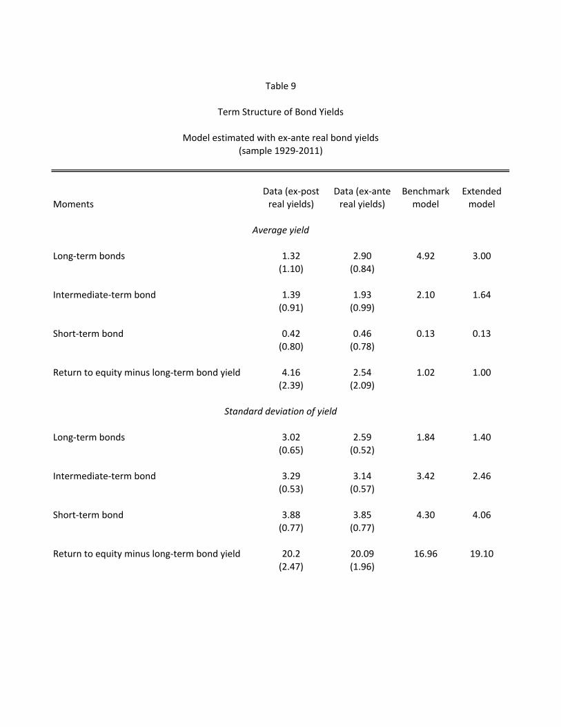
MomentsData*(ex-post*real*yields)

Data*(ex-ante*real*yields)

Benchmark*model

Extended*model

Long-term*bonds 1.32 2.90 4.92 3.00(1.10) (0.84)

Intermediate-term*bond 1.39 1.93 2.10 1.64(0.91) (0.99)

Short-term*bond 0.42 0.46 0.13 0.13(0.80) (0.78)

Return*to*equity*minus*long-term*bond*yield 4.16 2.54 1.02 1.00(2.39) (2.09)

Long-term*bonds 3.02 2.59 1.84 1.40(0.65) (0.52)

Intermediate-term*bond 3.29 3.14 3.42 2.46(0.53) (0.57)

Short-term*bond 3.88 3.85 4.30 4.06(0.77) (0.77)

Return*to*equity*minus*long-term*bond*yield 20.2 20.09 16.96 19.10(2.47) (1.96)

Table*9

Term*Structure*of*Bond*Yields

Model*estimated*with*ex-ante*real*bond*yields

Average'yield

Standard'deviation'of'yield

(sample*1929-2011)

Sample Mean Zero,lags,in,weighting,matrix

12,lags,in,weighting,matrix

5,year,minus,2.5,year 1985<2015, 0.19 0.03 0.101985<2006.Q3 0.09 0.03 0.11

10,year,minus,2.5,year 1985<2015, 0.38 0.05 0.171985<2006.Q3 0.22 0.05 0.17

15,year,minus,2.5,year 1985<2015 0.42 0.06 0.201985<2006.Q3 0.26 0.06 0.19

20,year,minus,2.5,year 1985<2015, 0.42 0.08 0.261985<2006.Q3 0.24 0.08 0.27

Table,10

Difference,between,long<term,yields,and,2.5,year,yieldsInflation<indexed,U.K.,gilts

Newey<West,standard,errors

Data$1929(2011 Benchmark$model Extended$model

R(square 0.03 0.13 0.03

Slope 0.91 3.48 0.98(0.46)

R(square 0.02 0.07 0.02

Slope 0.72$ 3.36 1.01(0.51)

Table$11

Regressions$of$Excess$Stock$Returns$on$Long(term$Bond$Yields$in$Excess$of$Short$Rate

Long%term*government*bonds*(20*years)

Intermediate*term*government*bonds*(5*years)

Model$estimated$with$ex(ante$real$bond$yields

8. Appendix

8.1. Appendix A

In this appendix, we solve the model in Section 3 analytically for the case of CRRA utility.

Let Ca,t denote the consumption of the representative agent at time t. The representative

agent solves the following problem:

Ut = maxEt

1X

i=0

δiλt+iC1−γa,t+i

1− γ,

subject to the flow budget constraints

Wa,i+1 = Rc,i+1 (Wa,i − Ca,i) ,

for all i ≥ t. The variable Rc,i+1 denotes the gross return to a claim that pays the aggregate

consumption as in equation (3.8), financial wealth is Wa,i = (Pc,i + Ci)Sa,i, and Sa,i is the

number of shares on the claim to aggregate consumption held by the representative agent.

The first-order condition for Sa,t+i+1 is:

δiλt+iC−γa,t+i = Et

"δi+1λt+i+1C

−γa,t+i+1Rc,i+1

#.

In equilibrium, Ca,t = Ct, Sa,t = 1. The equilibrium value of the intertemporal marginal

rate of substitution is:

Mt+1 = δλt+1λt

&Ct+1Ct

'−γ. (8.1)

The Euler equation for stock returns is the familiar,

Et [Mt+1Rc,t+1] = 1.

We now solve for Pc,t. It is useful to write Rc,t+1 as

Rc,t+1 =(Pc,t+1/Ct+1 + 1)

Pc,t/Ct

&Ct+1Ct

'.

In equilibrium:

Et

*Mt+1

&Pc,t+1Ct+1

+ 1

'&Ct+1Ct

'+=Pc,tCt. (8.2)

Replacing the value of Mt+1 in equation (8.2):

Et

"δλt+1λt

&Ct+1Ct

'−γ &Pc,t+1Ct+1

+ 1

'&Ct+1Ct

'#=Pc,tCt.

37

Using the fact that λt+1/λt is known as of time t we obtain:

δλt+1λtEt

*exp

"µ+ σc"

ct+1

#1−γ&Pct+1Ct+1

+ 1

'+=PctCt.

We guess and verify that Pct+1/Ct+1 is independent of "ct+1. This guess is based on the

fact that the model’s price-consumption ratio is constant absent time-preference shocks.

Therefore,

δλt+1λt

exp((1− γ)µ+ (1− γ)2 σ2c/2

)Et

&Pc,t+1Ct+1

+ 1

'=Pc,tCt. (8.3)

We now guess that there are constants k0, k1,..., such that

Pc,tCt

= k0 + k1 (λt+1/λt) + k2 (λt+1/λt)1+ρ + k3 (λt+1/λt)

1+ρ+ρ2 + ... (8.4)

Using this guess,

Et

&Pc,t+1Ct+1

+ 1

'

= Et

.k0 + k1

"(λt+1/λt)

ρ exp"σλ"

λt+1

##+ k2

"(λt+1/λt)

ρ exp"σλ"

λt+1

##1+ρ+ ...+ 1

/

= k0 + k1 (λt+1/λt)ρ exp

"σ2λ/2

#+ k2 (λt+1/λt)

ρ(1+ρ) exp"(1 + ρ)2 σ2λ/2

#+ ...+ 1. (8.5)

Substituting equations (8.4) and (8.5) into equation (8.3) and equating coe¢cients leads to

the following solution for the constants ki:

k0 = 0,

k1 = δ exp((1− γ)µ+ (1− γ)2 σ2c/2

),

and for n ≥ 2

kn = kn1 exp

nh1 + (1 + ρ)2 +

"1 + ρ+ ρ2

#2+ ...+

"1 + ...+ ρn−2

#2iσ2λ/2

o.

We assume that the series kn converges, so that the equilibrium price-consumption ratio

is given by equation (8.4). Hence, the realized return on the consumption claim is

Rc,t+1 =Ct+1Ct

k1 (λt+2/λt+1) + k2 (λt+2/λt+1)1+ρ + ...+ 1

k1 (λt+1/λt) + k2 (λt+1/λt)1+ρ + ...

. (8.6)

The equation that prices the one-period risk-free asset is:

Et [Mt+1Rf,t+1] = 1.

38

Taking logarithms of both sides of this equation and noting that Rf,t+1 is known at time t,

we obtain:

rf,t+1 = − logEt (Mt+1) .

Using equation (8.1),

Et (Mt+1) = δλt+1λtEt(exp

"−γ"µ+ σc"

ct+1

##)

= δλt+1λt

exp"−γµ+ γ2σ2c/2

#.

Therefore,

rf,t+1 = − log (δ)− log (λt+1/λt) + γµ− γ2σ2c/2.

Using equation (3.4), we obtain

E((λt+1/λt)

−1) = exp&σ2λ/2

1− ρ2

'.

We can then write the unconditional risk-free rate as:

E (Rf,t+1) = exp

&σ2λ/2

1− ρ2

'δ−1 exp(γµ− γ2σ2c/2).

Thus, the equity premium is given by:

E [(Rc,t+1)−Rf,t+1] = exp&σ2λ/2

1− ρ2

'δ−1 exp(γµ− γ2σ2c/2)

(exp

"γσ2c#− 1),

which can be written as:

E [(Rc,t+1)−Rf,t+1] = E (Rf,t+1)(exp

"γσ2c#− 1).

8.2. Appendix B

This appendix provides a detailed derivation of the equilibrium of the model economy where

the representative agent has Epstein-Zin preferences and faces time-preference shocks. The

agent solves the following problem:

U (Wt) = maxCt

hλtC

1−1/ t + δ

"U∗t+1

#1−1/ i1/(1−1/ ), (8.7)

where U∗t+1 =(Et"U (Wt+1)

1−γ#)1/(1−γ). The optimization is subject to the following budgetconstraint:

Wt+1 = Rc,t+1 (Wt − Ct) .

39

The agent takes as given the stochastic processes for the return on the consumption claim

Rc,t+1 and the preference shock λt+1. For simplicity, we omit the dependence of life-time

utility on the processes for λt+1 and Rc,t+1.

The first-order condition with respect to consumption is,

λtC−1/ t = δ

"U∗t+1

#−1/ (Et"U (Wt+1)

1−γ#)1/(1−γ)−1Et"U (Wt+1)

−γ U 0 (Wt+1)Rc,t+1#,

and the envelope condition is:

U 0 (Wt) = U (Wt)1/ δ

"U∗t+1

#−1/ (Et"U (Wt+1)

1−γ#)1/(1−γ)−1Et"U (Wt+1)

−γ U 0 (Wt+1)Rc,t+1#.

Combining the first-order condition and the envelope condition we obtain:

U 0 (Wt) = U (Wt)1/ λtC

−1/ t . (8.8)

This equation can be used to replace the value of U 0 (Wt+1) in the first order condition:

λtC−1/ t = δ

"U∗t+1

#−1/ (Et"U (Wt+1)

1−γ#)1/(1−γ)−1Et.U (Wt+1)

1/ −γ λt+1C−1/ t+1 Rc,t+1

/.

Using the expression for U∗t+1, this last equation can be written after some algebra as,

1 = Et (Mt+1Rc,t+1) . (8.9)

Here, Mt+1 is the stochastic discount factor, or intertemporal marginal rate of substitution,

which is given by:

Mt+1 = δλt+1λt

U (Wt+1)1/ −γ

"U∗t+1

#1/ −γC−1/ t+1

C−1/ t

.

We guess and verify the policy function for consumption and the form of the utility

function. As in Weil (1989) and Epstein and Zin (1991), we guess that:

U (Wt) = atWt,

Ct = btWt.

Replacing these guesses in equation (8.8) and simplifying yields:

a1−1/ t = λtb

−1/ t . (8.10)

Using the same guesses in the Hamilton-Jacobi-Bellman equation (8.7) and simplifying, we

obtain:

at =

2

64λtb1−1/ t + δ

0

@"Et

&at+1

Wt+1

Wt

'1−γ!#1/(1−γ)1

A1−1/

3

75

1/(1−1/ )

.

40

Finally, using the budget constraint to replace Wt+1/Wt we obtain:

at =

*λtb

1−1/ t + δ

.(Et"(at+1 (1− bt)Rc,t+1)

1−γ#)1/(1−γ)/1−1/ +1/(1−1/ )

. (8.11)

Equations (8.10) and (8.11) give a solution to at and bt.

Combining equations (8.10) and (8.11) we obtain:

λtb−1/ t (1− bt) = δ

.(Et"(at+1 (1− bt)Rc,t+1)

1−γ#)1/(1−γ)/1−1/ ,

which we can replace in the expression for the stochastic discount factor together with (8.10)

to obtain:

Mt+1 =

&δλt+1λt

'(1−γ)/(1−1/ )&bt+1bt(1− bt)

'−((1/ −γ)/ )/(1−1/ )&Ct+1Ct

'−1/ (Rc,t+1)

1/ −γ .

Now note that θ = (1− γ) / (1− 1/ ), and that

Ct+1Ct

Rc,t+1=bt+1Rc,t+1 (Wt − Ct) / (btWt)

Rc,t+1=bt+1 (1− bt)

bt,

to finally get,

Mt+1 =

&δλt+1λt

'θ &Ct+1Ct

'− θ

(Rc,t+1)θ−1 .

Taking logarithms of both sides and equating the consumption of the representative agent

to aggregate consumption yields equation (3.9).

The rest of the equilibrium derivation involves solving for rc,t+1, rd,t+1, and rf,t+1. Un-

til this point, we did not need to specify the process for the time-preference, consumption

growth, and dividend growth shocks. We solve the rest of the model assuming the general

processes of Subsection 3.4 given in equations (3.21) through (3.24). Recovering the equi-

librium values for the benchmark model is easily done by setting πcΛ = πdΛ = ση = 0 and

ν = σw = αc = αd = ρc = ρd = 0.

To price the consumption claim, we must solve the pricing condition:

Et [exp (mt+1 + rc,t+1)] = 1.

We guess that the logarithm of the price consumption ratio, zct ≡ log (Pc,t/Ct), is

zct = Ac0 + Ac1xt + Ac2ηt+1 + Ac3σ2t + Ac4∆ct,

and approximate

rc,t+1 = κc0 + κc1zct+1 − zct +∆ct+1. (8.12)

41

Replacing the approximation and the guessed solution for zct on the pricing condition gives

Et [exp (θ log (δ) + θ log (λt+1/λt) + (1− γ)∆ct+1 + θκc0 + θκc1zct+1 − θzct)] = 1.

Computing this expectation requires some algebra and yields the equation

0 = θ log (δ) + (1− γ + θκc1Ac4)µc − (1− γ + θκc1Ac4)αcσ2 + ((1− γ + θκc1Ac4)αc + θκc1Ac3) (1− ν)σ2

+((1− γ + θκc1Ac4) πcΛ + θκc1Ac1σΛ)2 /2 + (θκc1Ac2)

2 /2 + ((1− γ + θκc1Ac4)αc + θκc1Ac3)2 σ2w/2

+θxt + θκc1Ac1ρxt − θAc1xt + θσηηt+1 − θAc2ηt+1 + (1− γ + θκc1Ac4) ρc∆ct − θAc4∆ct − θAc0

+((1− γ + θκc1Ac4)αc + θκc1Ac3) vσ2t − θAc3σ

2t + (1− γ + θκc1Ac4)

2 σ2t/2 + θκc1Ac0 + θκc0.

In equilibrium, this equation must hold in all possible states resulting in the restrictions:

Ac1 =1

1− κc1ρ,

Ac2 = ση,

Ac3 =αcv +

(1−γ)/21−κc1ρc

1− κc1v

1− 1/ 1− κc1ρc

,

Ac4 =(1− 1/ ) ρc1− κc1ρc

,

and

Ac0 =log (δ) + (1− 1/ + κc1Ac4) (µc − αcσ

2) + κc0 + ((1− 1/ + κc1Ac4)αc + κc1Ac3) (1− ν)σ2

1− κc1

+θ ((1− 1/ + κc1Ac4) πcΛ + κc1Ac1σΛ)

2 /2 + θ (κc1Ac2)2 /2 + θ ((1− 1/ + κc1Ac4)αc + κc1Ac3)

2 σ2w/2

1− κc1.

To solve for the risk-free rate, we again use the stochastic discount factor to price the

risk-free asset. In logarithms, the Euler equation is:

rf,t+1 = − log (Et (exp (mt+1)))

= − log&Et

&exp

&θ log (δ) + θ log (λt+1/λt)−

θ

∆ct+1 + (θ − 1) rc,t+1

'''.

Using equation (8.12), we get:

rf,t+1 = − log (Et (exp (θ log (δ) + θ log (λt+1/λt)− γ∆ct+1 + (θ − 1) (κc0 + κc1zct+1 − zct)))) .

42

Substituting in the consumption process and the solution for the price-consumption ratio,

and after much algebra, we obtain,

rf,t+1 = −θ log (δ) + γ1µc − γ1αcσ2 − (θ − 1)κc0 − (θ − 1)κc1Ac0 − ((θ − 1)κc1Ac3 − γ1αc) (1− ν)σ2

+(θ − 1)Ac0 − ((θ − 1)κc1Ac1σΛ − γ1πcΛ)2 /2− ((θ − 1)κc1Ac2)

2 /2− ((θ − 1)κc1Ac3 − γ1αc)2 σ2w/2

−xt − σηηt+1 + (1/ ) ρc∆ct − ((θ − 1)κc1Ac3 − γ1αc) vσ2t + (θ − 1)Ac3σ

2t − γ21σ

2t/2,

where

γ1 = γ − (θ − 1)κc1Ac4.

Setting πcΛ = πdΛ = ση = 0 and ν = σw = αc = αd = ρc = ρd = 0 = 0, we get the

benchmark-model value of the risk-free rate (3.18).

Finally, we price a claim to dividends. Again, we assume the price-dividend ratio is given

by

zdt = Ad0 + Ad1xt + Ad2ηt+1 + Ad3σ2t + Ad4∆ct + Ad5∆dt,

and approximate the log-linearized return to the claim to the dividend:

rd,t+1 = κd0 + κd1zdt+1 − zdt +∆dt+1. (8.13)

The pricing condition is

Et [exp (mt+1 + rd,t+1)] = 1.

Using the expressions for mt+1, rc,t+1 and rd,t+1,

1 = Et

*exp θ log (δ) + θ log (λt+1/λt)−

θ

∆ct+1 + (θ − 1) (κc0 + κc1zct+1 − zct +∆ct+1)

+κd0 + κd1zdt+1 − zdt +∆dt+1] .

Replacing the consumption and dividend growth processes and of the price-consumption and

price-dividend ratios, and solving for the expectations, we obtain:

Ad1 =1

1− κd1ρ,

Ad2 = ση,

Ad4 =− (1/ ) ρc1− κd1ρc

,

Ad5 =ρd

1− κd1ρd,

43

Ad3 =(1 + κd1Ad5)αdv − bγαcv −

.αcv +

1−γ1−κc1ρc

/2/

1/ −γ1−κc1ρc

+ (1 + κd1Ad5)2 σ2d/2 + ((1 + κd1Ad5) πdc − bγ)

2 /2

1− κd1v,

where

bγ = γ − (θ − 1)κc1Ac4 − κd1Ad4,

and

Ad0 (1− κd1) = θ log (δ)− bγµc + (1 + κd1Ad5)µd − ((1 + κd1Ad5)αd − bγαc)σ2 + (θ − 1)κc0 + (θ − 1)κc1Ac0 + κd0

+((1 + κd1Ad5)αd − bγαc + (θ − 1)κc1Ac3 + κd1Ad3) (1− v)σ2 + ((θ − 1)κc1Ac2 + κd1Ad2)2 /2

+ ((1 + κd1Ad5) πdΛ − bγπcΛ + ((θ − 1)κc1Ac1 + κd1Ad1)σΛ)2 /2

+ ((1 + κd1Ad5)αd − bγαc + (θ − 1)κc1Ac3 + κd1Ad3)2 σ2w/2− (θ − 1)Ac0.

Equality of the long run mean of consumption growth and of dividend growth requires that

µc1− ρc

=µd

1− ρd.

Having solved for these constants, we can compute the expected return on the dividend

claim, Et (rd,t+1). Setting the relevant parameters to zero, we obtain the benchmark-model

value of Et (rd,t+1) given in equation (3.17). The expression for the conditional risk premium

in the benchmark model can be obtained by solving:

Et (rd,t+1)− rf,t+1 = Et (κd0 + κd1zdt+1 − zdt +∆dt+1)− rf,t+1.

8.3. Appendix C

In this appendix we solve for the prices of zero-coupon bonds of di§erent maturities. Again,

we present the equilibrium prices for the model of Subsection 3.4. Recovering the equilibrium

values for the benchmark model is easily done by setting πcΛ = πdΛ = ση = 0 and ν = σw =

αc = αd = ρc = ρd = 0. Let P (n)t be the time-t price of a bond that pays one unit of

consumption at t+n, with n ≥ 1. The Euler equation for the one-period risk-free bond price

P(1)t = 1/Rf,t+1 is

P(1)t = Et (Mt+1) .

The price for a risk-free bond maturing in n > 1 periods can be written recursively as:

P(n)t = Et

.Mt+1P

(n−1)t+1

/.

44

In Appendix B we derive the value of the risk-free rate:

rf,t+1 = − lnhP(1)t

i.

It is useful to write the risk-free rate as:

rf,t+1 = − log&λt+1λt

'+ (1/ ) ρc∆ct − p

1 − q1σ2t ,

where

p1 = θ log (δ)− γ1µc + γ1αcσ2 + (θ − 1)κc0 + (θ − 1)κc1Ac0 − (θ − 1)Ac0

+((θ − 1)κc1Ac3 − γ1αc) (1− ν)σ2

+((θ − 1)κc1Ac2)2 /2 + ((θ − 1)κc1Ac1σΛ − γ1πcΛ)

2 /2

+ ((θ − 1)κc1Ac3 − γ1αc)2 σ2w/2,

and

q1 = γ21/2 + ((θ − 1)κc1Ac3 − γ1αc) v − (θ − 1)Ac3.

Let p(n)t = lnhP(n)t

i. Therefore,

p(1)t = −rf,t+1

= p1 + xt + σηηt+1 − (1/ ) ρc∆ct + q1σ2t .

We now compute the price of a risk-free bond that pays one unit of consumption in two

periods:

p(2)t = lnEt

hexp

.mt+1 + p

(1)t+1

/i.

Using the expression formt+1 and the solution for rc,t+1 and zct we obtain, after much algebra,

p(2)t = p2 + (1 + ρ) xt + σηηt+1 + q2σ

2t − (γ2ρc + (θ − 1)Ac4)∆ct,

with

γ2 = γ1 + (1/ ) ρc,

p2 = θ log (δ)− γ2µc + γ2αcσ2 + (θ − 1)κc0 + (θ − 1)κc1Ac0 − (θ − 1)Ac0

+((θ − 1)κc1Ac3 − γ2αc + q1) (1− ν)σ2

+((θ − 1)κc1Ac2 + ση)2 /2 + (((θ − 1)κc1Ac1 + 1) σΛ − γ2πcΛ)

2 /2

+ (−γ2αc + (θ − 1)κc1Ac3 + q1)2 σ2w/2 + p

1,

45

q2 = γ22/2 + ((θ − 1)κc1Ac3 − γ2αc) v − (θ − 1)Ac3 + vq1.

Following the same procedure, we obtain the general formula for n ≥ 2:

p(n)t = pn +

"1 + ρ+ ...+ ρn−1

#xt + σηηt+1 + qnσ

2t − (γnρc + (θ − 1)Ac4)∆ct,

where:

qn = γ2n/2 + ((θ − 1)κc1Ac3 − γnαc) v − (θ − 1)Ac3 + νqn−1,

pn = θ log (δ)− γnµc + γnαcσ2 + (θ − 1)κc0 + (θ − 1)κc1Ac0 − (θ − 1)Ac0

+((θ − 1)κc1Ac3 − γnαc + qn−1) (1− ν)σ2

+((θ − 1)κc1 + 1)2 σ2η/2 +

""(θ − 1)κc1Ac1 +

"1 + ρ+ ...+ ρn−2

##σΛ − γnπcΛ

#2/2

+ ((θ − 1)κc1Ac3 − γnαc + qn−1)2 σ2w/2 + p

n−1,

with p1 and q1 given above, and the sequence of γ given by

γn = γ1"1 + ρc + ...+ ρn−2c

#+ (1/ ) ρn−1c +

"1 + ρc + ...+ ρn−3c

#(θ − 1)Ac4

...

γ3 = γ1 (1 + ρc) + (1/ ) ρ2c + (θ − 1)Ac4

γ2 = γ1 + (1/ ) ρc

γ1 = γ − (θ − 1)κc1Ac4.

Finally, we define the yield on an n-period zero-coupon bond as y(n)t = − 1np(n)t .

8.4. Appendix D

This Appendix contains a set of tables that provide versions of the results dicussed in the

main text that use ex-post, instead of ex-ante versions of the real interest rate.

46

Parameter Benchmark,model Extended,model Parameter Benchmark,model Extended,model

γ 1.7005 2.2228 ρ 0.99143 0.99108(0.017871) (0.22671) (0.00047649) (0.00059552)

ψ 1.4623 2.3876 σλ 0.00054228 0.00040323,(0.043679) (0.62451) ,(2.0143e?05) (2.6299e?05)

δ 0.99784 0.9978 Implied value of θ ?2.2158 ?2.1041,(0.0021963) ,(0.00013075) (0.099733) ,(0.50544)

σc 0.0068554 0.0046005 ν 0.00 0.99673(0.00015674) ,(0.00046367) ,(0.00057417)

µ 0.0015234 0.0009117 σω 0.00 1.70E?06,(5.2956e?05) (5.7211e?05) ,(2.6272e?07)

πcλ 0.00 ?0.0018895 αc 0.00 ?119.3912(0.00029618) (28.7094)

σd 0.017153 0.025564 αd 0.00 ?145.5293(0.00041145) (0.52335) (68.6766)

πdc 0.0015658 ?1.3161 ρc 0.00 0.090348(0.00041998) (0.80412) (0.045439)

πdλ 0.00 ?0.010369 ρd 0.00 0.33438(0.0054912) (0.39606)

ση 0.00 0.0082606(0.00043981)

Table 4 (appendix)

Parameter Estimates and Standard ErrorsModels estimated with ex-post real bond yields

Moments(Matched(in(EstimationData((constrained,(

ex4post(bond(yields)

Data((unconstrained,(ex4post(bond(yields)

Benchmark(model Extended(model

Average(growth(rate(of( 1.4941 2.2197 1.84 1.20of(consumption (0.30395) (0.22413)

Average(growth(rate(of(dividends 1.4941 0.12538 1.84 1.20(0.30395) (0.65732)

Standard(deviation(of(the(growth 2.1865 2.1624 2.36 2.72rate(of(consumption (0.34494) ((0.31345)

Standard(deviation(of(the(growth 6.914 6.5181 5.89 6.95rate(of(dividends ((1.0409) ((1.1219)

Contemporaneous(correlation 0.2215 0.23722 0.09 0.21between(consumption(growth(and ((0.1006) (0.10649)dividend(growth

First4order(serial(correlation 0.2001 0.1584 40.01 0.43of(consumption (0.1475) (0.1240)

Correlation(between(stock(returns 40.1555 40.2607 0.00 40.04(and(one4period(lagged(consumption(growth(0.1070) (0.0999)

Correlation(between(stock(returns 0.4950 0.5093 0.01 0.22(and(one4period(lead(consumption(growth(0.0670) (0.0490)

Average(return(to(equities 7.8252 6.3948 6.25 3.87(1.74) (1.8804)

Standard(deviation(of(return(to 17.2537 17.6831 15.93 16.67equities (1.3783) (1.461)

Average(risk4free(rate 0.19347 0.10476 0.19 0.19(0.84341) (0.84457)

Standard(deviation(of(the(risk4free 3.4656 3.5054 3.99 4.23rate (0.82769) (0.83489)

First4order(serial(correlation(of(the 0.59242 0.59736 0.90 0.49risk4free(rate (0.082348) (0.078284)

Equity(premium 7.6318 6.29 6.06 3.68(1.758) (1.8812)

Average(price4dividend(ratio 3.3761 3.3775 3.12 3.30(0.14887) (0.14887)

Standard(deviaton(of(price4 0.47324 0.44502 0.28 0.40dividend(ratio (0.074827) (0.081116)

First4order(serial(correlation(of 0.95041 0.93257 0.84 0.89price(dividend(ratio (0.034499) (0.042679)

Contemporaneous(correlation 0.20139 0.21274 40.95 40.24between(risk(free(rate(and (0.12648)( (0.12982)(price(dividend(ratio

Table(5((appendix)

Models estimated with ex-post real bond yields

Moments

Data*(constrained)

Data*(unconstrained)

Benchmark*model Extended*model

19year*correlation*between 90.07 90.05 0.04 90.14equity*returns*and (0.11) *(0.12)consumption*growth

59year*correlation*between 90.01 90.05 0.05 0.01equity*returns*and (0.16) (0.13)consumption*growth

109year*correlation*between 90.08 90.21 0.05 0.18equity*returns*and *(0.30) (0.21)consumption*growth

19year*correlation*between 0.08 0.05 0.37 90.11equity*returns*and *(0.11) *(0.11)dividend*growth

59year*correlation*between 0.22 0.29 0.35 0.07equity*returns*and *(0.14) *(0.14)dividend*growth

109year*correlation*between 0.51 0.59 0.41 0.26equity*returns*and *(0.22) (0.15)dividend*growth

Table*6*(appendix)

Model*estimated*with*ex9post*bond*returns

Dividend'growth

Consumption'growth

Correlation*Between*Stock*Returns*and*Per*CapitaGrowth*Rates*of*Consumption*and*Dividends

DataModel)(median)

Model)(plim) Data

Model)(median)

Model)(plim)

R1square (%)of)values)larger)thanR1square)in)data)

1)year 10.10 10.05 0.008 0.08 0.01 0.0003)(0.03) (0.02)

3)years 10.27 10.14 0.027 0.14 0.03 0.001(0.07) (0.08)

5)years 10.41 10.21 0.034 0.26 0.04 0.001)(0.12) (0.04)

1)year 10.10 10.06 10.03 0.08 0.02 0.01)(0.03) (0.05)

3)years 10.27 10.18 10.08 0.14 0.06 0.02(0.07) (0.19)

5)years 10.41 10.26 10.13 0.26 0.09 0.04)(0.12) (0.12)

Predictability)of)Excess)Returns)by)Price1dividend)Ratio)at)Various)Horizons

Table)7)(apendix)

Benchmark*model

Slope)coefficient

Extended*model

Model)estimated)with)ex1post)real)bond)yields

Sample Full)sample Pre-1983 Post-1983

Canada 1952)2014 0.02 0.55 )0.31(0.14) (0.06) (0.25)

France 1932)2014 )0.56 )0.67 0.07(0.17) (0.13) (0.17)

Germany 1968)2014 )0.11 )0.10 )0.20(0.08) (0.13) (0.20)

Italy 1940)2014 )0.54 )0.63 0.35(0.14) (0.08) (0.21)

Japan 1960)2014 0.39 )0.01 0.66(0.16) (0.20) (0.08)

U.K. 1934)2014 0.32 0.27 )0.25(0.11) (0.06) (0.22)

US 1939)2011 0.21274 0.172 )0.44(0.12982)- (0.148) -(0.21)

Correlation-of-price)dividend-ratio-and-ex)post-risk)free-rate

Table-8-(appendix)

MomentsData*(ex-post*real*yields)

Data*(ex-ante*real*yields)

Benchmark*model

Extended*model

Long-term*bonds 1.32 2.90 5.30 2.53(sample*1929-1992) (1.10) (0.84)

Intermediate-term*bond 1.39 1.93 2.25 1.53(sample*1929-2007) (0.91) (0.99)

Short-term*bond 0.42 0.46 0.19 0.19(sample*1929-2011) (0.80) (0.78)

Return*to*equity*minus*long-term*bond*yield 4.16 2.54 0.95 1.34(sample*1929-1992) (2.39) (2.09)

Long-term*bonds 3.02 2.59 1.73 1.39(sample*1929-1992) (0.65) (0.52)

Intermediate-term*bond 3.29 3.14 3.19 2.49(sample*1929-2007) (0.53) (0.57)

Short-term*bond 3.88 3.85 3.99 4.23(sample*1929-2011) (0.77) (0.77)

Return*to*equity*minus*long-term*bond*yield 20.2 20.09 15.59 16.53(sample*1929-1992) (2.47) (1.96)

Table*9*(appendix)

Term*Structure*of*Bond*Yields

Model*estimated*with*ex-post*yields

Average'yield

Standard'deviation'of'yield

Data$1929(2011 Benchmark$model Extended$model

R(square 0.02 0.12 0.04

Slope 0.60 3.40 0.97(0.96)

R(square 0.002 0.07 0.03

Slope (0.30 3.30 0.97(1.10)

Long%term*government*bonds*(20*years)

Intermediate*term*government*bonds*(5*years)

Regressions$of$Excess$Stock$Returns$on$Long(term$Bond$Yields$in$Excess$of$Short$Rate

Table$11$(appendix)

Model$estimated$with$ex(post$real$yields

τ-10 -8 -6 -4 -2 0 2 4 6 8 10

-1

-0.8

-0.6

-0.4

-0.2

0

0.2

0.4

0.6

0.8

1United States - Correlogram of Returns (t) and Consumption Growth (t+ τ)

Figure 1: Correlograms of stock returns and fundamentals

Panel A

τ-10 -8 -6 -4 -2 0 2 4 6 8 10

-1

-0.8

-0.6

-0.4

-0.2

0

0.2

0.4

0.6

0.8

1United States - Correlogram of Returns (t) and GDP Growth (t+ τ)

τ-10 -5 0 5 10

-1

-0.5

0

0.5

1Canada: corr(rt, ∆ct+τ)

τ-10 -5 0 5 10

-1

-0.5

0

0.5

1Canada: corr(rt, ∆yt+τ)

τ-10 -5 0 5 10

-1

-0.5

0

0.5

1France: corr(rt, ∆ct+τ)

τ-10 -5 0 5 10

-1

-0.5

0

0.5

1France: corr(rt, ∆yt+τ)

τ-10 -5 0 5 10

-1

-0.5

0

0.5

1Italy: corr(rt, ∆ct+τ)

Figure 1: Correlograms of stock returns and fundamentals

Panel B

τ-10 -5 0 5 10

-1

-0.5

0

0.5

1Italy: corr(rt, ∆yt+τ)

τ-10 -5 0 5 10

-1

-0.5

0

0.5

1Germany: corr(rt, ∆ct+τ)

τ-10 -5 0 5 10

-1

-0.5

0

0.5

1Germany: corr(rt, ∆yt+τ)

τ-10 -5 0 5 10

-1

-0.5

0

0.5

1Japan: corr(rt, ∆ct+τ)

τ-10 -5 0 5 10

-1

-0.5

0

0.5

1Japan: corr(rt, ∆yt+τ)

τ-10 -5 0 5 10

-1

-0.5

0

0.5

1United Kingdom: corr(rt, ∆ct+τ)

Figure 1: Correlograms of stock returns and fundamentals

Panel C

τ-10 -5 0 5 10

-1

-0.5

0

0.5

1United Kingdom: corr(rt, ∆yt+τ)