Valuation Risk and Asset Pricing∗

Rui Albuquerque†, Martin Eichenbaum‡, and Sergio Rebelo§

November 2013

Abstract

Standard representative-agent models have diffi culty in accounting for the weakcorrelation between stock returns and measurable fundamentals, such as consumptionand output growth. This failing underlies virtually all modern asset-pricing puzzles.The correlation puzzle arises because these models load all uncertainty onto the supplyside of the economy. We propose a simple theory of asset pricing in which demandshocks play a central role. These shocks give rise to valuation risk that allows themodel to account for key asset pricing moments, such as the equity premium, the bondterm premium, and the weak correlation between stock returns and fundamentals.

J.E.L. Classification: G12.Keywords: Equity premium, bond yields, risk premium.

∗We benefited from the comments and suggestions of Fernando Alvarez, Frederico Belo, JaroslavBorovicka, Lars Hansen, Anisha Ghosh, Ravi Jaganathan, Tasos Karantounias, Junghoon Lee, JonathanParker, Costis Skiadas, and Ivan Werning. We thank Robert Barro, Emi Nakamura, Jón Steinsson, andJosé Ursua for sharing their data with us and Benjamin Johannsen for superb research assistance. Albu-querque gratefully acknowledges financial support from the European Union Seventh Framework Programme(FP7/2007-2013) under grant agreement PCOFUND-GA-2009-246542. A previous version of this paperwas presented under the title “Understanding the Equity Premium Puzzle and the Correlation Puzzle,”http://tinyurl.com/akfmvxb.

†Boston University, Portuguese Catholic University, CEPR, and ECGI.‡Northwestern University, NBER, and Federal Reserve Bank of Chicago.§Northwestern University, NBER, and CEPR.

1. Introduction

In standard representative-agent asset-pricing models, the expected return to an asset re-

flects the covariance between the asset’s payoff and the agent’s stochastic discount factor.

An important challenge to these models is that the correlation and covariance between

stock returns and measurable fundamentals, especially consumption growth, is weak at both

short and long horizons. Cochrane and Hansen (1992), Campbell and Cochrane (1999), and

Cochrane (2001) call this phenomenon the correlation puzzle. More recently, Lettau and Lud-

vigson (2011) document this puzzle using different methods. According to their estimates,

the shock that accounts for the vast majority of asset-price fluctuations is uncorrelated with

consumption at virtually all horizons.

The basic disconnect between measurable macroeconomic fundamentals and stock re-

turns underlies virtually all modern asset-pricing puzzles, including the equity-premium

puzzle, Hansen-Singleton (1982)-style rejection of asset-pricing models, violation of Hansen-

Jagannathan (1991) bounds, and Shiller (1981)-style observations about excess stock-price

volatility. It is also at the root of the high estimates of risk aversion and correspondingly

enormous amounts that agents would pay for early resolution of uncertainty in long-run risk

models of the type proposed by Bansal and Yaron (2004) (see Epstein, Farhi, and Strzalecki

(2013)).

A central finding of modern empirical finance is that variation in asset returns is over-

whelmingly due to variation in discount factors (see Cochrane (2011)). A key question is:

how should we model this variation? In classic asset-pricing models, all uncertainty is loaded

onto the supply side of the economy. In Lucas (1978) tree models, agents are exposed to

random endowment shocks, while in production economies they are exposed to random pro-

ductivity shocks. Both classes of models abstract from shocks to the demand for assets.

Not surprisingly, it is very diffi cult for these models to simulateneously account for key asset

pricing phenomena like the equity premium puzzle and the correlation puzzle.

We propose a simple theory of asset pricing in which demand shocks, arising from sto-

chastic changes in agents’rate of time preference, play a central role in the determination

of asset prices. These shocks amount to a parsimonious way of modeling the variation in

discount rates stressed by Cochrane (2011). An important implication of our model is that

the law of motion for these shocks play a first-order role in determining the equilibrium

behavior of objects like the price-dividend ratio. As a result, our analysis is disciplined the

1

fact that the law of motion for preference shocks must be consistent with the time-series

properties of variables like the price-dividend ratio.

In our model, the representative agent has recursive preferences of the type considered

by Kreps and Porteus (1978), Weil (1989), and Epstein and Zin (1991). Time-preference

shocks help account for the equity premium as long as the risk-aversion coeffi cient and

the elasticity of intertemporal substitution are either both greater than one or both are

smaller than one. When the risk-aversion coeffi cient is equal to the inverse of the elasticity

of intertemporal substitution, recursive preferences reduce to constant-relative risk aversion

(CRRA) preferences. We show that, in this case, time-preference shocks have negligible

effects on key asset-pricing moments such as the equity premium.

We estimate our model using data over the sample period 1929 to 2011. The condition for

time-preference shocks to help explain the equity premium puzzle is always satisfied in the

different versions of the model that we estimate. Taking sampling uncertainty into account,

our model accounts for the equity premium and the volatility of stock and bond returns,

even though the estimated degree of agents’risk aversion is very moderate (roughly one).

Critically, the model also accounts for the time series of the price-dividend ratio as well as

the correlation between stock returns and fundamentals such as consumption, output, and

dividend growth at short, medium and long horizons. The model can also account for the

observed predictability of excess returns by lagged price-dividend ratios.

We define valuation risk as the risk associated with changes in the way that future cash

flows are discounted due to time-preference shocks. According to our estimates, valuation

risk is a much more important source of variation in asset prices than conventional covariance

risk. The model has no diffi culty in accounting for the average rate of return to stocks and

bonds. But, absent preference shocks, our model implies that stocks and bonds should, on

average, have very similar rates of return.

Valuation risk is an increasing function of an asset’s maturity. So, a natural test of our

model is whether it can account for the bond term premia and the return on stocks relative

to long-term bonds. We pursue this test using stock returns as well as ex-post real returns

on bonds of different maturity and argue that the model’s implications are consistent with

the data. We are keenly aware of the limitations of the available data on real bond returns,

especially at long horizons. Still, we interpret our results as being very supportive of the

hypothesis that valuation risk is a critical determinant of asset prices.

2

There is a literature that models shocks to the demand for assets as arising from time-

preference or taste shocks. For example, Garber and King (1983) and Campbell (1986)

consider these types of shocks in early work on asset pricing. Tesar and Stockman (1995)

and Pavlova and Rigobon (2007) study the role of taste shocks in explaining asset prices in

an open economy model. In the macroeconomic literature, Eggertsson and Woodford (2003),

Eggertsson (2004), model changes in savings behavior as arising from time-preference shocks

that make the zero lower bound on nominal interest rates binding.1 A common property of

these papers is that agents have CRRA preferences. In independent work, contemporaneous

with our own, Maurer (2012) explores the impact of time-preference shocks in a calibrated

continuous-time representative agent model with Duffi e-Epstein (1992) preferences.2

The key contribution of our paper is empirical. We consider two main variants of our

model. In both versions consumption follows a martingale with conditionally homoscedastic

shocks. These models account for the predictability of excess returns by past price-dividend

ratios as an artifact of small-sample bias.

In the first variant of the model, time-preference shocks are uncorrelated with endowment

shocks. This variant is very useful for highlighting the basic role of demand shocks in asset

pricing. In a production economy, these shocks would generally induce changes in aggregate

output and consumption. To assess the robustness of our results to this possibility, we

consider a variant of the model that allows endowment and time-preference shocks to be

correlated.

Our paper is organized as follows. In Section 2 we document the correlation puzzle using

U.S. data for the period 1929-2011 as well as the period 1871-2006. In Section 3 we present

our benchmark model where time-preference shocks are uncorrelated with the growth rate

of consumption. We discuss our estimation strategy and present our benchmark empirical

results in Section 4. In Section 5 we present the variant of our model in which time-preference

shocks are correlated with consumption shocks and its empirical performance. In Section 6

we study the empirical implications of the model for bond term premia, as well as the return

1See also Huo and Rios-Rull (2013), Correia, Farhi, Nicolini, and Teles (2013), and Fernandez-Villaverde,Guerron-Quintana, Kuester, Rubio-Ramírez (2013).

2Normandin and St-Amour (1998) study the impact of preference shocks in a model similar to ours.Unfortunately, their analysis does not take into account the fact that covariances between asset returns,consumption growth, and preferences shocks depend on the parameters governing preferences and technology.As a result, their empirical estimates imply that preference shocks decrease the equity premium. In addition,they argue that they can explain the equity premium with separable preferences and preference shocks. Thisclaim contradicts the results in Campbell (1986) and the theorem in our Appendix B.

3

on stocks relative to long-term bonds. In Section 7 we study the predictability of excess

stock returns by the price-dividend ratio. Section 8 concludes.

2. The correlation puzzle

In this section we examine the correlation between stock returns and fundamentals as mea-

sured by the growth rate of consumption, output, dividends, and earnings.

2.1. Data sources

We consider two sample periods: 1929 to 2011 and 1871 to 2006. For the first sample,

we obtain nominal stock and bond returns from Kenneth French’s website. We convert

nominal returns to real returns using the rate of inflation as measured by the consumer

price index. We use the measure of consumption expenditures and real per capita Gross

Domestic Product constructed by Barro and Ursua (2011), which we update to 2011 using

National Income and Product Accounts data. We compute per-capita variables using total

population (POP).3 We obtain data on real S&P500 earnings and dividends from Robert

Shiller’s website. We use data from Ibbotson and Associates on the real return to one-

month Treasury bills, intermediate-term government bonds (with approximate maturity of

five years), and long-term government bonds (with approximate maturity of twenty years).

For the second sample, we use data on real stock and bond returns from Nakamura,

Steinsson, Barro, and Ursua (2010) for the period 1870-2006. We use the same data sources

for consumption, expenditures, dividends and earnings as in the first sample.

As in Mehra and Prescott (1985) and the associated literature, we measure the risk-

free rate using realized real returns on nominal, one-year Treasury Bills. This measure is

far from perfect because there is inflation risk, which can be substantial, particularly for

long-maturity bonds.

3This series is not subject to a very important source of measurement error that affects another commonly-used population measure, civilian noninstitutional population (CNP16OV). Every ten years, the CNP16OVseries is adjusted using information from the decennial census. This adjustment produces large discontinuitiesin the CNP16OV series. The average annual growth rates implied by the two series are reasonably similar:1.2 for POP and 1.4 for CNP16OV for the period 1952-2012. But the growth rate of CNP16OV is threetimes more volatile than the growth rate of POP. Part of this high volatility in the growth rate of CNP16OVis induced by large positive and negative spikes that generally occur in January. For example, in January2000, 2004, 2008, and 2012 the annualized percentage growth rates of CNP16OV are 14.8, −1.9, −2.8, and8.4, respectively. The corresponding annualized percentage growth rates for POP are 1.1, 0.8, 0.9, and 0.7.

4

2.2. Empirical results

Table 1, panel A presents results for the sample period 1929-2011. We report correlations

at the one-, five- and ten-year horizons. The five- and ten-year horizon correlations are

computed using five- and ten-year overlapping observations, respectively. We report Newey-

West (1987) heteroskedasticity-consistent standard errors computed with ten lags.

There are three key features of Table 1, panel A. First, consistent with Cochrane and

Hansen (1992) and Campbell and Cochrane (1999), the growth rate of consumption and

output are uncorrelated with stock returns at all the horizons that we consider. Second, the

correlation between stock returns and dividend growth is similar to that of consumption and

output growth at the one-year horizon. However, the correlation between stock returns and

dividend growth is substantially higher at the five and ten-year horizons than the analogue

correlations involving consumption and output growth. Third, the pattern of correlations

between stock returns and dividend growth are similar to the analogue correlations involving

earnings growth.

Table 1, panel B reports results for the longer sample period (1871-2006). The one-

year correlation between stock returns and the growth rates of consumption and output

are very similar to those obtained for the shorter sample. There is evidence in this sample

of a stronger correlation between stock returns and the growth rates of consumption and

output at a five-year horizon. But, at the ten-year horizon the correlations are, once again,

statistically insignificant. The results for dividends and earnings are very similar across the

two subsamples.

Table 2 assesses the robustness of our results for the correlation between stock returns

and consumption using three different measures of consumption for the period 1929-2011,

obtained from the National Product and Income Accounts. With one exception, the corre-

lations in this table are statistically insignificant. The exception is the one-year correlation

between stock returns and the growth rate of nondurables and services which is marginally

significant.

In summary, there is remarkably little evidence that the growth rates of consumption or

output are correlated with stock returns. There is also little evidence that dividends and

earnings are correlated with stock returns at short horizons.

We have focused on correlations because we find them easy to interpret. One might be

concerned that a different pictures emerges from the pattern of covariances between stock

5

returns and fundamentals. It does not. For example, using quarterly U.S. data for the period

1959 to 2000, Parker (2001) argues that one would require a risk aversion coeffi cient of 379

to account for the equity premium given his estimate of the covariance between consumption

growth and stock returns. Parker (2001) observes that there is a larger covariance between

current stock returns and the cumulative growth rate of consumption over the next 12

quarters. However, even with this covariance measure he shows that one would require

a risk aversion coeffi cient of 38 to rationalize the equity premium.

Viewed overall, the results in this section serve as our motivation for introducing shocks

to the demand for assets. Classic asset-pricing models load all uncertainty onto the supply-

side of the economy. As a result, they have diffi culty in simultaneously accounting for the

equity premium and the correlation puzzle. This diffi culty is shared by the habit-formation

model proposed by Campbell and Cochrane (1999) and the long-run risk models proposed

by Bansal and Yaron (2004) and Bansal, Kiku, and Yaron (2012). Rare-disaster models

of the type proposed by Rietz (1988) and Barro (2006) also share this diffi culty because

all shocks, disaster or not, are to the supply side of the model. A model with a time-

varying disaster probability, of the type consider by Wachter (2012) and Gourio (2012),

might be able to rationalize the low correlation between consumption and stock returns

as a small sample phenomenon. The reason is that changes in the probability of disasters

induces movements in stock returns without corresponding movements in actual consumption

growth. This force lowers the correlation between stock returns and consumption in a sample

where rare disasters are under represented. This explanation might account for the post-war

correlations. But we are more skeptical that it accounts for the results in Table 1, panel B,

which are based on the longer sample period, 1871 to 2006.

Below, we focus on demand shocks as the source of the low correlation between stock

returns and fundamentals, rather than the alternatives just mentioned. We model these

demand shocks in the simplest possible way by introducing shocks to the time preference of

the representative agent. These shocks can be thought of as capturing changes in agents’

attitudes towards savings, such as those emphasized by Eggertsson and Woodford (2003).

These shocks can also reflect changes in institutional factors, such as the tax treatment

of retirement plans. Finally, these shocks could also capture the effects of changes in the

demographics of stock market participants (see Geanakoplos, Magill, and Quinzii (2004)).

In Appendix A we provide a simple example of an overlapping-generations model in which

6

uncertainty about the growth rate of the population gives rise to shocks in the demand for

assets.

3. The benchmark model

In this section, we study the properties of a simple representative-agent endowment economy

modified to allow for time-preference shocks. The representative agent has the constant-

elasticity version of Kreps-Porteus (1978) preferences used by Epstein and Zin (1991) and

Weil (1989). The life-time utility of the representative agent is a function of current utility

and the certainty equivalent of future utility, U∗t+1:

Ut = maxCt

[λtC

1−1/ψt + δ

(U∗t+1

)1−1/ψ]1/(1−1/ψ)

, (3.1)

where Ct denotes consumption at time t and δ is a positive scalar. The certainty equivalent

of future utility is the sure value of t+ 1 lifetime utility, U∗t+1 such that:(U∗t+1

)1−γ= Et

(U1−γt+1

).

The parameters ψ and γ represent the elasticity of intertemporal substitution and the coef-

ficient of relative risk aversion, respectively. The ratio λt+1/λt determines how agents trade

off current versus future utility. We assume that this ratio is known at time t.4 We refer to

λt+1/λt as the time-preference shock.

3.1. Stochastic processes

To highlight the role of time-preference shocks, we adopt a very simple stochastic process

for consumption:

log(Ct+1) = log(Ct) + µ+ σcεct+1. (3.2)

Here, µ and σc are non-negative scalars and εct+1 follows an i.i.d. standard-normal distribu-

tion.

As in Campbell and Cochrane (1999), we allow dividends, Dt, to differ from consumption.

In particular, we assume that:

log(Dt+1) = log(Dt) + µ+ πdcεct+1 + σdε

dt+1. (3.3)

4We obtain similar results with a version of the model in which the utility function takes the form:

Ut =[C1−1/ψt + λtδ

(U∗t+1

)1−1/ψ]1/(1−1/ψ).

7

Here, εdt+1 is an i.i.d. standard-normal random variable that is uncorrelated with εct+1. To

simplify, we assume that the average growth rate of dividends and consumption is the same

(µ). The parameter σd ≥ 0 controls the volatility of dividends. The parameter πdc controls

the correlation between consumption and dividend shocks.5

The growth rate of the time-preference shock evolves according to:

log (λt+1/λt) = ρ log (λt/λt−1) + σλελt+1. (3.4)

Here, ελt+1 is an i.i.d. standard-normal random variable. In the spirit of the original Lucas

(1978) model, we assume, for now, that ελt+1 is uncorrelated with εct+1 and ε

dt+1. We relax

this assumption in Section 5. We assume that λt+1/λt is highly persistent but stationary

(ρ very close to one). The idea is to capture, in a parsimonious way, persistent changes in

agents’attitudes towards savings.

The CRRA case In Appendix B we solve the model analytically for the case in which

γ = 1/ψ. Here preferences reduce to the CRRA form:

Vt = Et

∞∑i=0

δiλt+iC1−γt+i , (3.5)

with Vt = U1−γt .

The unconditional risk-free rate is affected by the persistence of volatility of time-preference

shocks:

E (Rf,t+1) = exp

(σ2λ/2

1− ρ2

)δ−1 exp(γµ− γ2σ2

c/2).

The unconditional equity premium implied by this model is proportional to the risk-free

rate:

E (Rc,t+1 −Rf,t+1) = E (Rf,t+1)[exp

(γσ2

c

)− 1]. (3.6)

Both the average risk-free rate and the volatility of consumption are small in the data.

Moreover, the constant of proportionality in equation (3.6), exp (γσ2c) − 1, is independent

of σ2λ. So, time-preference shocks do not help to resolve the equity premium puzzle when

preferences are of the CRRA form.

5The stochastic process described by equations (3.2) and (3.3) implies that log(Dt+1/Ct+1) follows arandom walk with no drift. This implication is consistent with our data.

8

3.2. Solving the model

We define the return to the stock market as the return to a claim on the dividend process.

The realized gross stock-market return is given by:

Rd,t+1 =Pd,t+1 +Dt+1

Pd,t, (3.7)

where Pd,t denotes the ex-dividend stock price.

It is useful to define the realized gross return to a claim on the endowment process:

Rc,t+1 =Pc,t+1 + Ct+1

Pc,t, (3.8)

where Pc,t denotes the price of an asset that pays a dividend equal to aggregate consumption.

We use the following notation to define logarithm of returns on the dividend and consumption

claims, the logarithm of the price-dividend ratio, and the logarithm of the price-consumption

ratio:

rd,t+1 = log(Rd,t+1),

rc,t+1 = log(Rc,t+1),

zdt = log(Pd,t/Dt),

zct = log(Pc,t/Ct).

In Appendix C we show that the logarithm of the stochastic discount factor (SDF) implied

by the utility function defined in equation (3.1) is given by:

mt+1 = log(δ) + log(λt+1/λt)−1

ψ∆ct+1 + (1/ψ − γ) log(Ut+1/U

∗t+1). (3.9)

It is useful to rewrite this equation as:

mt+1 = θ log (δ) + θ log (λt+1/λt)−θ

ψ∆ct+1 + (θ − 1) rc,t+1, (3.10)

where θ is given by:

θ =1− γ

1− 1/ψ. (3.11)

When γ = 1/ψ, the case of CRRA preferences, the value of θ is equal to one and the

stochastic discount factor is independent of rc,t+1.

We solve the model using the approximation proposed by Campbell and Shiller (1988),

which involves linearizing the expressions for rc,t+1 and rd,t+1 and exploiting the properties

of the log-normal distribution.6

6See Hansen, Heaton, and Li (2008) for an alternative solution procedure.

9

Using a log-linear Taylor expansion we obtain:

rd,t+1 = κd0 + κd1zdt+1 − zdt + ∆dt+1, (3.12)

rc,t+1 = κc0 + κc1zct+1 − zct + ∆ct+1, (3.13)

where ∆ct+1 ≡ log (Ct+1/Ct) and ∆dt+1 ≡ log (Dt+1/Dt). The constants κc0, κc1, κd0, and

κd1 are given by:

κd0 = log [1 + exp(zd)]− κd1zd,

κc0 = log [1 + exp(zc)]− κc1zc,

κd1 =exp(zd)

1 + exp(zd), κc1 =

exp(zc)

1 + exp(zc),

where zd and zc are the unconditional mean values of zdt and zct.

The Euler equations associated with a claim to the stock market and a consumption

claim can be written as:

Et [exp (mt+1 + rd,t+1)] = 1, (3.14)

Et [exp (mt+1 + rc,t+1)] = 1. (3.15)

We solve the model using the method of undetermined coeffi cients. First, we replace

mt+1, rc,t+1 and rd,t+1 in equations (3.14) and (3.15), using expressions (3.12), (3.13) and

(3.10). Second, we guess and verify that the equilibrium solutions for zdt and zct take the

form:

zdt = Ad0 + Ad1 log (λt+1/λt) , (3.16)

zct = Ac0 + Ac1 log (λt+1/λt) . (3.17)

This solution has the property that price-dividend ratios are constant, absent movements

in λt. This property results from our assumption that the logarithm of consumption and

dividends follow random-walk processes. We compute Ad0, Ad1, Ac0, and Ac1 using the

method of indeterminate coeffi cients.

We show in Appendix C that the conditional expected return to equity is given by:

Et (rd,t+1) = − log (δ)− log (λt+1/λt) + µ/ψ (3.18)

+

[(1− θ)θ

(1− γ)2 − γ2

]σ2c/2 + πdc (2γσc − πdc) /2− σ2

d/2

+

(1− θ) (κc1Ac1) [2 (κd1Ad1)− (κc1Ac1)]− (κd1Ad1)2σ2λ/2.

10

Recall that κc1 and κd1 are non-linear functions of the parameters of the model.

We define the compensation for valuation risk as the part of the one-period expected

return to an asset that is due to the volatility of the time preference shock, σ2λ. We refer to

the part of the expected return that is due to the volatility of consumption and dividends

as the compensation for conventional risk.

For stocks, the compensation for valuation risk, vd, is given by the last term in equation

(3.18):

vd =[2 (1− θ) (κc1Ac1) (κd1Ad1)− (κd1Ad1)2 − (1− θ) (κc1Ac1)2]σ2

λ/2.

To gain intuition about the determinants of vd, it is useful to consider the simple case in

which the stock market is a claim on consumption. In this case vd is given by:

vd = −θ (κc1Ac1)2 σ2λ/2.

The compensation for valuation risk is positive as long as θ is negative. In terms of the

underlying structural parameters, this condition holds as long as γ > 1 and ψ > 1 or γ < 1

and ψ < 1.7 Put differently, if agents have a coeffi cient of risk aversion higher than one, the

condition requires that agents have a relatively high elasticity of intertemporal substitution.

Alternatively, if agents have a coeffi cient of risk aversion lower than one, they must have a

relatively low elasticity of intertemporal substitution. The value of θ is negative in all our

estimated models, so the value of vd is positive.

Using the Euler equation for the risk-free rate, rf,t+1,

Et [exp (mt+1 + rf,t+1)] = 1,

we obtain:

rf,t+1 = − log (δ)− log (λt+1/λt) + µ/ψ − (1− θ) (κc1Ac1)2 σ2λ/2 (3.19)

+

[(1− θ)θ

(1− γ)2 − γ2

]σ2c/2.

Equations (3.18) and (3.19) imply that the risk-free rate and the conditional expectation

of the return to equity are decreasing functions of log (λt+1/λt). When log (λt+1/λt) rises,

7The condition θ < 0 is different from the condition that guarantees preference for early resolution ofuncertainty: γ > 1/ψ, which is equivalent to θ < 1. As discussed in Epstein (2012), the latter conditionplays a crucial role in generating a high equity premium in long-run risk models. Because long-run risks areresolved in the distant future, they are more heavily penalized than current risks. For this reason, long-runrisk models can generate a large equity premium even when shocks to current consumption are small.

11

agents value the future more relative to the present, so they want to save more. Since risk-

free bonds are in zero net supply and the number of stock shares is constant, aggregate

savings cannot increase. So, in equilibrium, returns on bonds and equity must fall to induce

agents to save less.

The approximate response of asset prices to shocks, emphasized by Borovicka, Hansen,

Hendricks, and Scheinkman (2011) and Borovicka and Hansen (2011), can be directly inferred

from equations (3.18) and (3.19). The response of the return to stocks and the risk-free rate

to a time-preference shock corresponds to that of an AR(1) with serial correlation ρ.

Using equations (3.18) and (3.19) we can write the conditional equity premium as:

Et (rd,t+1)− rf,t+1 = πdc (2γσc − πdc) /2− σ2d/2 (3.20)

+κd1Ad1 [2 (1− θ)Ac1κc1 − κd1Ad1]σ2λ/2.

Since the constants Ac1, Ad1, κc1, and κd1 are all positive, θ < 1 is a necessary condition for

time-preference shocks to help explain the equity premium.

The component of the equity premium that is due to valuation risk is given by the last

term in equation (3.20). It is useful to consider the case in which the stock is a claim on

consumption. In this case, that term reduces to:

(1− 2θ)

(κc1

1− ρκc1

)2

σ2λ/2.

This expression is positive as long as one of the following conditions holds:

γ < 0.5(1 + 1/ψ) and ψ < 1,γ > 0.5(1 + 1/ψ) and ψ > 1.

(3.21)

As it turns out, this condition is always satisfied in the estimated versions of our model.

It is interesting to highlight the differences between time-preference shocks and conven-

tional sources of uncertainty, which pertain to the supply-side of the economy. Suppose that

there is no risk associated with the physical payoff of assets such as stocks. In this case,

standard asset pricing models would imply that the equity premium is zero. In our model,

there is a positive equity premium that results from the different exposure of bonds and

stocks to valuation risk. Agents are uncertain about how much they will value future divi-

dend payments. Since λt+1 is known at time t, this valuation risk is irrelevant for one-period

bonds. But, it is not irrelevant for stocks, because they have infinite maturity. In general,

the longer the maturity of an asset, the higher is its exposure to time-preference shocks and

the large is the valuation risk.

12

Finally, we conclude by considering the case in which there are supply-side shocks to

the economy but agents are risk neutral (γ = 0). In this case, the component of the equity

premium that is due to valuation risk is positive as long as ψ is less than one. The intuition

is as follows: stocks are long-lived assets whose payoffs can induce unwanted variation in the

period utility of the representative agent, λtC1−1/ψt . Even when agents are risk neutral, they

must be compensated for the risk of this unwanted variation.

3.3. Relation to long-run risk models

In this subsection we briefly comment on the relation between our model and the long-run-

risk model pioneered by Bansal and Yaron (2004). Both models emphasize low-frequency

shocks that induce large, persistent changes in the agent’s stochastic discount factor. To see

this point, it is convenient to re-write the representative agent’s utility function, (3.1), as:

Ut =[C

1−1/ψt + δ

(U∗t+1

)1−1/ψ]1/(1−1/ψ)

where Ct = λ1/(1−1/ψ)t Ct. Taking logarithms of this expression we obtain:

log(Ct

)= 1/ (1− 1/ψ) log(λt) + log (Ct)

Bansal and Yaron (2004) introduce a highly persistent component in the process for log(Ct),

which is a source of long-run risk. In contrast, we introduce a highly persistent component

into log(Ct) via our specification of the time-preference shocks. From equation (3.9), it

is clear that both specifications can induce large, persistent movements in mt+1. Despite

this similarity, the two models are not observationally equivalent. First, they have different

implications for the correlation between observed consumption growth, log(Ct+1/Ct) and

asset returns. Second, the two models have very different implications for the average return

to long-term bonds, and the term structure of interest rates. We return to these points when

we discuss our empirical results in Sections 5 and 6.

4. Estimating the benchmark model

We estimate the parameters of our model using the Generalized Method of Moments (GMM).

Our estimator is the parameter vector Φ that minimizes the distance between a vector of

empirical moments, ΨD, and the corresponding model population moments, Ψ(Φ).

We proceed as follows. We estimate ΨD, which includes the following 20 moments: the

mean and standard deviation of consumption growth, the mean and standard deviation of

13

dividend growth, the correlation between the one-year growth rate of dividends and the one-

year growth rate of consumption, the mean and standard deviation of real stock returns, the

mean, standard deviation and autocorrelation of the real risk-free rate, the mean, standard

deviation and autocorrelation of the price-dividend ratio, the correlation between stock re-

turns and the risk-free rate, the correlation between stock returns and consumption growth at

the one, five and ten-year horizon, the correlation between stock returns and dividend growth

at the one, five and ten-year horizon. The parameter vector Φ includes nine parameters: γ

(the coeffi cient of relative risk aversion), ψ (the elasticity of intertemporal substitution), δ

(the rate of time preference), σc (the volatility of innovation to consumption growth), πdc

(the parameter that controls the correlation between consumption and dividend shocks),

σd (the volatility of dividend shocks), ρ (the persistence of time-preference shocks), and σλ

(the volatility of the innovation to time-preference shocks), and µ (the mean growth rate of

dividends and consumption). We constrain the growth rate of dividends and consumption

to be the same. We estimate ΨD using a standard two-step effi cient GMM estimator with

a Newey-West (1987) weighting matrix that has ten lags. The latter matrix corresponds to

our estimate of the variance-covariance matrix of the empirical moments, ΩD.

We assume that agents make decisions at a monthly frequency and derive the model’s

implications for population moments computed at an annual frequency, Ψ(Φ). See Appendix

D for details.

We compute our estimator Φ as:

Φ = arg minΦ

[Ψ(Φ)−ΨD]′Ω−1D [Ψ(Φ)−ΨD] .

Table 3 reports our parameter estimates along with GMM standard errors. Several

features are worth noting. First, both the estimates of the coeffi cient of risk aversion and

the intertemporal elasticity of substitution are close to one. The point estimates satisfy the

condition θ < 1 which is necessary for time-preference shocks to help explain the equity

premium. The estimates also satisfy the more stringent condition (3.21), required for a

positive equity premium in the absence of consumption and dividend shocks. Second, the

estimate of θ is statistically significant at normal significance levels and so are the estimates

of γ and ψ. Third, the growth rate of λt is estimated to be highly persistent, with a first-

order serial correlation close to one (0.995). Fourth, the volatility of the innovation to the

growth rate of dividends is much higher than that of the innovation to the growth rate of

consumption. Finally, the estimate of δ is close to one.

14

Table 4 compares the moments implied by the benchmark model with the estimated data

moments. Recall that in estimating the model parameters we impose the restriction that

the unconditional average growth rate of consumption and dividends coincide. To assess the

robustness of our results to this restriction, we present two versions of the estimated data

moments, one that imposes this restriction and one that does not. With one exception, the

constrained and unconstrained moment estimates are similar, taking sampling uncertainty

into account. The exception is the average growth rate of consumption, where the constrained

and unconstrained estimates are statistically different.

Table 4 shows that the model generates a high average equity premium (5.14) and a low

average risk-free rate (0.77). Neither of these model moments is statistically different from

our estimates of the corresponding data moments. Even though the coeffi cient of relative

risk aversion is close to one, the model is consistent with the observed equity premium. This

result might seem surprising because our estimates of γ and 1/ψ are close to each other.

However, the implied value of θ, the key determinant of the equity premium, is −2.108.

The basic intuition for why our model generates a high equity premium despite a low

coeffi cient of relative risk aversion is as follows. From the perspective of the model, stocks

and bonds are different in two ways. First, the model embodies the conventional source of

an equity premium, namely bonds have a certain payoff that does not covary with the SDF

while the payoff to stocks covaries negatively with the SDF (as long as πdc > 0). Since γ is

close to one, this traditional covariance effect is very small. Second, the model embodies a

compensation for valuation risk that is particularly pronounced for stocks given their long-

lived nature relative to bonds. Recall that, given our timing assumptions, when an agent

buys a bond at t, the agent knows the value of λt+1, so the only source of risk are movements

in the marginal utility of consumption at time t + 1. In contrast, the time-t stock price

depends on the value of λt+j, for all j > 1. So, agents are exposed to valuation risk, a risk

that is particularly important because time-preference shocks are very persistent.

In Table 5 we decompose the equity premium into the valuation risk premium and the

conventional risk premium. We calculate these premia at the benchmark parameter estimates

using various values of ρ. Two key results emerge from this table. First, the conventional

risk premium is always roughly zero. This result is consistent with Kocherlakota’s (1996)

discussion of why the equity premium is not explained by endowment models in which

the representative agent has recursive preferences and consumption follows a martingale.

15

Second, consistent with the intuition discussed above, the valuation risk premium and the

equity premium are increasing in ρ. The larger is ρ, the more exposed agents are to large

movements in stock prices induced by time-preference shocks.

Implications for the correlation puzzle Table 6 reports the model’s implications for the

correlation of stock returns with consumption and dividend growth. Recall that consumption

and dividends follow a random walk. In addition, the estimated process for the growth rate

of the time-preference shock is close to a random walk. So, the correlation between stock

returns and consumption growth implied by the model is essentially the same across different

horizons. A similar property holds for the correlation between stock returns and dividend

growth.

The model does well at matching the correlation between stock returns and consumption

growth in the data, because this correlation is similar at all horizons. In contrast, the

empirical correlation between stock returns and dividend growth increases with the time

horizon. The estimation procedure chooses to match the long-horizon correlations and does

less well at matching the yearly correlation. This choice is dictated by the fact that it is

harder for the model to produce a low correlation between stock returns and dividend growth

than it is to produce a low correlation between stock returns and consumption growth. This

property reflects the fact that the dividend growth rate enters directly into the equation for

stock returns (see equation (3.12)).

Implications for the risk-free rate A problem with some explanations of the equity

premium is that they imply counterfactually high levels of volatility for the risk-free rate

(see e.g. Boldrin, Christiano and Fisher (2001)). Table 4 shows that the volatility of the

risk-free rate and stock market returns implied by our model are similar to the estimated

volatilities in the data. Notice also that, taking sampling uncertainty into account, the model

accounts for the correlation between the risk-free rate and stock returns.

An empirical shortcoming of the benchmark model is its implication for the persistence

of the risk-free rate. Recall that, according to equation (3.19), the risk-free rate has the same

persistence as the growth rate of the time-preference shock. Table 4 shows that the AR(1)

coeffi cient of the risk free rate, as measured by the ex-post realized real returns to one-year

treasury bills, is only 0.61, with a standard error of 0.11, which is substantially smaller that

our estimate of ρ (0.96). We address this issue in the next section.

16

5. Extensions of the benchmark model

In this section we present two extensions of the benchmark model. In the first extension

we present a simple perturbation of the benchmark model that renders it consistent with

the observed persistence of the risk free rate. We refer to this extension as the augmented

model. Second, we modify this extension to allow for correlation between time preference

shocks and the growth rate of consumption and dividends. We refer to this version as the

quasi-production model.

An important advantage of our benchmark model is its simplicity and its ability to

account for both the equity premium and the correlation puzzle with low risk aversion.

However, this model suffers from an important shortcoming: it overstates the persistence

of the risk-free rate. It is straightforward to resolve this issue by assuming that the time-

preference shock is the sum of a persistent shock and an i.i.d. shock:

log(λt+1/λt) = xt+1 + σηηt+1, (5.1)

xt+1 = ρxt + σλελt+1,

where ελt+1 and ηt+1 are uncorrelated, i.i.d. standard normal shocks. If ση = 0 and x1 =

log(λ1/λ0) we obtain the specification of the time-preference shock used in the benchmark

model. Other things equal, the larger is ση, the lower the persistence of the time-preference

shock.

We define the augmented model as a version of the benchmark model in which we replace

equation (3.4) with (5.1). We estimate the augmented model by adding ση to the vector Φ.

Tables 3 through 6 report our results. With the exception of ση, the estimated structural

parameters are very similar across the two models. With one important exception, the

models’implications for the data moments are also very similar, taking sampling uncertainty

into account. The exception pertains to the serial correlation of the risk-free rate that falls

from 0.96 in the benchmark model to 0.77 in the augmented model, a value that is within

two standard errors of the sample moment. According to our point estimates, the i.i.d.

component of the time-preference shock accounts for 80 percent of the variance of the shock.

We now turn to a more interesting shortcoming of the benchmark and augmented models:

they do not allow the growth rate of consumption and/or dividends to be correlated with

the time-preference shocks. In a production economy, time-preference shocks would gener-

ally induce changes in aggregate consumption. For example, in a simple real-business-cycle

17

model, a persistent increase in λt+1/λt would lead agents to reduce current consumption and

invest more in order to consume more in the future. Taken literally, an endowment economy

specification does not allow for such a correlation. We can, however, modify the augmented

model to mimic a production economy along this dimension by allowing the growth rate of

dividends, consumption and the time-preference shock to be correlated. We refer to this

extension as the quasi-production model.

We assume that the stochastic process for consumption and dividend growth is given by:

log(Ct+1) = log(Ct) + µ+ σcεct+1 + πcλε

λt+2, (5.2)

εct+1 ∼ N(0, 1),

log(Dt+1) = log(Dt) + µ+ πdcεct+1 + σdε

dt+1 + πdλε

λt+2,

εdt+1 ∼ N(0, 1),

where εct+1, εdt+1, ε

λt+1, and ηt+1 are mutually uncorrelated. As long as the two new parame-

ters, πcλ and πdλ are different from zero, log(λt+1/λt) is correlated with log(Ct+1/Ct) and

log(Dt+1/Dt). Only the innovation to time-preference shocks enters the law of motion for

log(Ct+1/Ct) and log(Dt+1/Dt). So, we are not introducing any element of long-run risk

into consumption or dividend growth. As in the benchmark and augmented models, both

consumption and dividends are martingales.

In estimating the model we add πcλ, πdλ, and ση to the vector Φ. Table 3 reports our point

estimates. As in the benchmark model, γ and ψ are still close to one and are statistically

significant at normal significance levels. First, the point estimates continue to satisfy the

condition θ < 1, required for time-preference shocks to generate an equity premium. The

value of θ is still large (equal to −2.35) and statistically significant. Second, even though

ρ continues to be close to one, the growth of λt is less persistent than in the benchmark

model because of the i.i.d. shock in equation (5.1). The values of πcλ are πdλ are negative

and statistically significant. Below we argue that these values allow the model to match the

yearly correlation between stock returns and dividend growth.

Tables 4 through 6 report the implications of the quasi-production model for various data

moments. A number of features are worth noting. First, this version of the model generates

a similar equity premium to that in the benchmark model (5.32 percent versus 5.14 percent).

Second, the average risk-free rate implied by the model is lower (0.18) and closer to the point

18

estimate in the data. Third, the volatility of stock returns and the risk-free rate implied by

the model are close to the point estimates. Fourth, taking sampling uncertainty into account,

the model accounts for the correlation between the risk-free rate and stock returns. Fifth,

the persistence of the risk-free rate implied by the model matches that in the data accounting

for sampling uncertainty.

Recall that the benchmark model produces correlations between stock returns and con-

sumption growth that are similar to those in the data. The quasi-production model continues

to succeed on this dimension by setting the πcλ to a value that is close to zero. The coeffi -

cient πdλ allows the model to fit the low level of the one-year and the five-year correlations

between stock returns and dividend growth. The cost is that the model does less well than

the benchmark model at matching the ten-year correlation. The reason the estimation pro-

cedure chooses to match the one-year and five-year correlations is that these correlations are

estimated with more precision than the ten-year correlation.

To document the relative importance of the correlation puzzle and the equity premium

puzzle, we re-estimate the model subject to the constraint that it matches the average equity

premium and the average risk-free rate. We report our results in Tables 3, 4 and 6. Even

though the estimates of γ and ψ are similar to those reported before, the implied value of

θ goes from −2.35 to −3.71, which is why the equity premium implied by the model rises.

This version of the model continues to produce low correlations between stock returns and

consumption growth. However, the one-year correlation between stock returns and dividend

growth implied by the model is much higher than that in the data (0.56 versus 0.08). The

one-year correlation between stock returns and dividend growth is estimated much more

precisely than the equity premium. So, the estimation algorithm chooses parameters for

the quasi-production model that imply a lower equity premium in return for matching the

one-year correlation between stock returns and dividend growth.

We conclude by highlighting an important difference between our model and long-run risk

models. For concreteness, we focus on the recent version of the long-run risk model proposed

by Bansal, Kiku, and Yaron (2012). Working with their parameter values, we find that the

correlation between stock returns and consumption growth are equal to 0.66, 0.88, and 0.92

at the one-, five- and ten-year horizon, respectively. Their model also implies correlations

between stock returns and dividend growth equal to 0.66, 0.90, and 0.93 at the one-, five-

and ten-year horizon, respectively. Our estimates reported in Table 1 imply that both sets

19

of correlations are counterfactually high. The source of this empirical shortcoming is that

all the uncertainty in the long-run risk model stems from the endowment process.

6. Bond term premia

As we emphasize above, the equity premium in our estimated models results primarily from

the valuation risk premium. Since this valuation premium increases with the maturity of an

asset, a natural way to assess the plausibility of our model is to evaluate its implications for

the slope of the real yield curve.

Table 7 reports the mean and standard deviation of ex-post real yields on short-term (one-

month) Treasury Bills, intermediate-term government bonds (with approximate maturity of

five years), and long-term government bonds (with approximate maturity of twenty years).

A number of features are worth noting. First, consistent with Alvarez and Jermann (2005),

the term structure of real yields is upward sloping. Second, the real yield on long-term bonds

is positive. This result is consistent with Campbell, Shiller and Viceira (2009) who report

that the real yield on long-term TIPS has always been positive and is usually above two

percent.

Our model implies that long-term bonds command a positive risk premium that increases

with the maturity of the bond (see Appendix E for details on the pricing of long term bonds).

The latter property reflects the fact that longer maturity assets are more exposed to valuation

risk. Table 7 shows that, taking sampling uncertainty into account, both the augmented and

the quasi-production model are consistent with the observed mean yields for short- and

intermediate-term bonds, but generate slightly larger yields on long-term bonds than in the

data. The table also shows that the estimated models account for the volatility of the returns

on short-, intermediate-, and long-term bonds. So, our model can account for key features

of the intermediate and long-term bond returns, even though these models were not used to

estimate the model.

According to Table 7, the augmented and quasi-production models imply that the differ-

ence between stock returns and long-term bond yields is roughly 2 percent. This value is well

within two standard errors of our point estimate. From the perspective of our model, the

positive premium that equity commands over long-term bonds reflects the difference between

an asset of infinite and twenty-year maturity. Consistent with this perspective, Binsbergen,

Hueskes, Koijen, and Vrugt (2011) estimate that 90 (80) percent of the value of the S&P

20

500 index corresponds to dividends that accrue after the first 5 (10) years.

Piazzesi and Schneider (2007) and Beeler and Campbell (2012) argue that the bond term

premium and the yield on long-term bonds are useful for discriminating between compet-

ing asset pricing models. For example, they stress that long-run risk models, of the type

pioneered by Bansal and Yaron (2004), imply negative long-term bond yields and a nega-

tive bond term premium. The intuition is as follows: in a long-run risk model agents are

concerned that consumption growth may be dramatically lower in some future state of the

world. Since bonds promise a certain payout in all states of the world, they offer insurance

against this possibility. The longer the maturity of the bond, the more insurance it offers

and the higher is its price. So, the term premium is downward sloping. Indeed, the return

on long-term bonds may be negative. Beeler and Campbell (2012) show that the return on

a 20-year real bond in the Bansal, Kiku and Yaron (2012) model is −0.88.

Standard rare-disaster models also imply a downward sloping term structure for real

bonds and a negative real yield on long-term bonds. See, for example the benchmark model

in Nakamura, Steinsson, Barro, and Ursúa (2010). According to these authors, these impli-

cations can be reversed by introducing the possibility of default on bonds and to assume that

probability of partial default is increasing in the maturity of the bond.8 So, we cannot rule

out the possibility that other asset-pricing models can account for bond term premia and

the rate of return on long-term bonds. Still, it seems clear that valuation risk is a natural

explanation of these features of the data.

We conclude with an interesting observation made by Binsbergen, Brandt, and Koijen

(2012). Using data over the period 1996 to 2009, these authors decompose the S&P500 index

into portfolios of short-term and long-term dividend strips. The first portfolio entitles the

holder to the realized dividends of the index for a period of up to three years. The second

portfolio is a claim on the remaining dividends. Binsbergen et al (2012) find that the short-

term dividend portfolio has a higher risk premium than the long-term dividend portfolio, i.e.

there is a negative stock term premium. They argue that this observation is inconsistent with

habit-formation, long-run risk models and standard of rare-disaster models.9 Our model, too,

8Nakamura et al (2010) consider a version of their model in which the probability of partial default ona perpetuity is 84 percent, while the probability of partial default on short-term bonds is 40 percent. Thismodel generates a positive term premium and a positive return on long-term bonds.

9Recently, Nakamura et al (2012) show that a time-vaying rare disaster model in which the componentof consumption growth due to a rare disaster follows an AR(1) process, is consistent with the Binsbergenet al (2012) results. Belo et al. (2013) show that the Binsbergen et al. (2012) result can be reconciled in avariety of models if the dividend process is replaced with processes that generate stationary leverage ratios.

21

has diffi culty in accounting for the Binsbergen et al (2012) negative stock term premium.

Of course, our sample is very different from theirs and their negative stock term premium

result is heavily influenced by the recent financial crisis (see Binsbergen et al (2011)). Also,

Boguth, Carlson, Fisher, and Simutin (2012) argue that the Binsbergen et al (2012) results

may be significantly biased because of the impact of small pricing frictions.

7. Excess return predictability

Table 8 presents evidence reproducing the well-known finding that excess returns are pre-

dictable based on lagged price-dividend ratios. Specifically, we report the results of regressing

excess-equity returns over holding periods of 1, 3 and 5 years on the lagged price-dividend

ratio. The slope coeffi cients are −0.09, −0.26 and −0.39, respectively, while the R-squares

are 0.04, 0.13 and 0.23, respectively. In our simple model, consumption is a martingale

with conditionally homoscedastic innovations. So by construction excess returns are unpre-

dictable in population. However, Stambaugh (1999) and Boudoukh et al. (2008) argue that

the apparent predictability of excess returns may be an artifact of small-sample bias. To pur-

sue this hypothesis, we take as the data generating process our estimated quasi-production

model and generate 50,000 artificial data sets. Each data set is monthly and spans 85 years.

We convert each monthly data sets into 85 annual observations. We then estimate the pre-

dictive regressions on each of the artificial data sets. Table 8 reports the median estimate of

the slope coeffi cients and R-squares. Note that the slope coeffi cients are −0.04, −0.12 and

−0.20, respectively, with standard deviations across the artificial data sets equal to 0.06,

0.16 and 0.24,respectively. So in each case, the point estimate from the data is contained

within a two-standard deviation band of the median Monte Carlo point estimate. Also note

that the median R-squares for the 1, 3 and 5 year predictive regressions on the artificial data

sets are 0.01, 0.03 and 0.05, respectively (these R-squares are comparable to those reported

in Bansal et al. (2012) on predictive regressions using the long run risk model). The fraction

of R-squares in the Monte Carlo data sets greater than or equal to the R-squares from the

predictive regressions in the actual data are 13.1%, 9.8% and 7.1%. Taken together we con-

clude there is relatively little evidence against the view that our simple model can account

for the slopes and R-squares in the predictive regressions estimated from the actual US data.

The question of whether predictability is a small sample phenomenon is diffi cult and a

full analysis is beyond the scope of this paper. However, we do two simple exercises in the

22

spirit of Brennan and Xia (2005) that suggest the predictive power of the price-dividend ratio

may be spurious in the sense stressed by Boudoukh et al. (2008). In particular we redo the

predictive regressions using two alternative right-hand variables: the stock-price divided by

aggregate per capita consumption (price-consumption ratio) and the stock price divided by

a deterministic series that grows at a constant rate equal to the mean dividend growth rate

(price-trend ratio). The results are reported in Table 8. Notice that the slope coeffi cients and

R-squares are very similar to those obtained with the price-dividend ratio. In our view, this

result casts some doubt on the economic significance of the predictive regressions obtained

with the price-dividend ratio.

8. Conditional Heteroscedasticity in Consumption

TBA

9. Conclusion

In this paper we argue that allowing for demand shocks in an otherwise standard asset pricing

model substantially improves the performance of the model. Specifically, it allows the model

to account for the equity premium, bond term premia, and the correlation puzzle with low

degrees of estimated risk aversion. According to our estimates, valuation risk is by far the

most important determinant of the equity premium and the bond term premia.

The recent literature has incorporated many interesting features into standard asset-

pricing models to improve their performance. Prominent examples, include habit formation,

long-run risk, time-varying endowment volatility, and model ambiguity. We abstract from

these features to isolate the empirical role of valuation risk. But they are, in principle,

complementary to valuation risk and could be incorporated into our analysis. We leave this

task for future research.

23

References

[1] Alvarez, Fernando, and Urban J. Jermann, “Using Asset Prices to Measure the Persis-

tence of the Marginal Utility of Wealth,”Econometrica, 73 (6): 1977—2016, 2005.

[2] Bansal, Ravi, and Amir Yaron. “Risks for the Long Run: A Potential Resolution of

Asset Pricing Puzzles,”The Journal of Finance, 59, n. 4: 1481-1509, 2004.

[3] Bansal, Ravi, Dana Kiku and Amir Yaron “An Empirical Evaluation of the Long-Run

Risks Model for Asset Prices,”Critical Finance Review, 1: 183—221, 2012.

[4] Barro, Robert J. “Rare Disasters and Asset Markets in the Twentieth Century,”Quar-

terly Journal of Economics, 121:823—66, 2006.

[5] Barro, Robert J., and José F. Ursua, “Rare Macroeconomic Disasters,”working paper

No. 17328, National Bureau of Economic Research, 2011.

[6] Beeler, Jason and John Y. Campbell, “The Long-Run Risks Model and Aggregate Asset

Prices: An Empirical Assessment,”Critical Finance Review, 1: 141—182, 2012.

[7] Belo, Frederico, Pierre Collin-Dufresne and Robert S. Goldstein, “Dividend Dynamics

and the Term Structure of Dividend Strips,”working paper, University of Minnesota,

2013.

[8] Binsbergen, Jules H. van, Michael W. Brandt, and Ralph S.J. Koijen “On the Timing

and Pricing of Dividends,”American Economic Review,102 (4), 1596-1618, June 2012.

[9] Binsbergen, Jules H. van, Wouter Hueskes, Ralph Koijen and Evert Vrugt “Equity

Yields,”National Bureau of Economic Research, working paper N. 17416, 2011.

[10] Boldrin, Michele, Lawrence J. Christiano, and Jonas Fisher “Habit Persistence, Asset

Returns, and the Business Cycle,”American Economic Review, 149-166, 2001.

[11] Borovicka, Jaroslav, Lars Peter Hansen “Examining Macroeconomic Models through

the Lens of Asset Pricing,”manuscript, University of Chicago, 2011.

[12] Borovicka, Jaroslav, Lars Peter Hansen, Mark Hendricks, and José A. Scheinkman

“Risk-price dynamics,”Journal of Financial Econometrics 9, no. 1: 3-65, 2011.

24

[13] Boguth, Oliver, Murray Carlson, Adlai Fisher and Mikhal Simutin “Leverage and the

Limits of Arbitrage Pricing: Implications for Dividend Strips and the Term Structure

of Equity Risk Premia,”manuscript, Arizona State University, 2012.

[14] Boudoukh, Jacob, Matthew Richardson and Robert F. Whitelaw, “The Myth of Long-

Horizon Predictability,”Review of Financial Studies 24, no. 4: 1577-1605.

[15] Brennan, Michael J., and Yihong Xia, “tay’s as good as cay,”Finance Research Letters

2, 1:14, 2005.

[16] Campbell, John Y. “Bond and Stock Returns in a Simple Exchange Model,”The Quar-

terly Journal of Economics 101, no. 4: 785-803, 1986.

[17] Campbell, John Y., and Robert J. Shiller “The Dividend-price Ratio and Expectations

of Future Dividends and Discount Factors,”Review of Financial Studies 1, no. 3: 195-

228, 1988.

[18] Campbell, John Y., and John H. Cochrane “By Force of Habit: A Consumption-based

Explanation of Aggregate Stock Market Behavior,”Journal of Political Economy, 107,

2: 205-251, 1999.

[19] Campbell, John, Robert Shiller and Luis Viceira “Understanding Inflation-Indexed

Bond Markets,”Brookings Papers on Economic Activity, 79-120, 2009.

[20] Cochrane, John H., Asset Pricing, Princeton University Press, 2001.

[21] Cochrane, John H. and Lars Peter Hansen “Asset Pricing Explorations for Macroeco-

nomics,”NBER Macroeconomics Annual 1992, Volume 7, pp. 115-182. MIT Press, 1992.

[22] Cochrane, John H. “Presidential Address: Discount Rates,”The Journal of Finance

66.4: 1047-1108, 2011.

[23] Correia, Isabel, Emmanuel Farhi, Juan Pablo Nicolini, and Pedro Teles “Unconventional

Fiscal Policy at the Zero Bound,”American Economic Review, 103(4): 1172-1211, 2013

[24] Duffi e, Darrell, and Larry G. Epstein “Stochastic Differential Utility,”Econometrica,

353-394, 1992.

25

[25] Eggertsson, Gauti “Monetary and Fiscal Coordination in a Liquidity Trap,”Chapter

3 of Optimal Monetary and Fiscal Policy in the Liquidity Trap, Ph.D. dissertation,

Princeton University, 2004.

[26] Eggertsson, Gauti B., and Michael Woodford “Zero Bound on Interest Rates and Op-

timal Monetary Policy”Brookings Papers on Economic Activity 2003, no. 1: 139-233,

2003.

[27] Epstein, Larry G. “How Much Would You Pay to Resolve Long-Run Risk?,”mimeo,

Boston University, 2012.

[28] Epstein, Larry G., and Stanley E. Zin “Substitution, Risk Aversion, and the Tempo-

ral Behavior of Consumption and Asset Returns: An Empirical Analysis,”Journal of

Political Economy, 263-286, 1991.

[29] Fernandez-Villaverde, Jesus, Pablo Guerron-Quintana, Keith Kuester, Juan Rubio-

Ramírez, “Fiscal Volatility Shocks and Economic Activity,”manuscript, University of

Pennsylvania, 2013.

[30] Garber, Peter M. and Robert G. King “Deep Structural Excavation? A Critique of

Euler Equation Methods,”National Bureau of Economic Research Technical Working

Paper N. 31, Nov. 1983.

[31] Geanakoplos, John, Michael Magill, and Martine Quinzii “Demography and the Long-

Run Predictability of the Stock Market,”Brookings Papers on Economic Activity 1:

241—307, 2004.

[32] Gourio, François “Disaster Risk and Business Cycles,” American Economic Review,

102(6): 2734-2766, 2012.

[33] Hansen, Lars Peter, John C. Heaton, and Nan Li, “Consumption Strikes Back? Mea-

suring Long-Run Risk,”Journal of Political Economy 116, no. 2: 260-302, 2008.

[34] Hansen, Lars Peter, and Ravi Jagannathan “Implications of Security Market Data for

Models of Dynamic Economies,”Journal of Political Economy 99, no. 2: 225-262, 1991.

[35] Hansen, Lars Peter, and Kenneth J. Singleton “Generalized Instrumental Variables Es-

timation of Nonlinear Rational Expectations Models,”Econometrica: 1269-1286, 1982.

26

[36] Kreps, David M., and Evan L. Porteus “Temporal Resolution of Uncertainty and Dy-

namic Choice Theory,”Econometrica, 185-200, 1978.

[37] Kocherlakota, Narayana R. "The Equity Premium: It’s Still a Puzzle," Journal of

Economic Literature, 42-71, 1996.

[38] Lettau, Martin and Sydney C. Ludvigson “Shocks and Crashes,”manuscript, New York

University, 2011.

[39] Lucas Jr, Robert E. “Asset Prices in an Exchange Economy,”Econometrica, 1429-1445,

1978.

[40] Maurer, Thomas A. “Is Consumption Growth Merely a Sideshow in Asset Pricing?,”

manuscript, London School of Economics, 2012.

[41] Mehra, Rajnish, and Edward C. Prescott “The Equity Premium: A Puzzle,” Journal

of Monetary Economics 15, no. 2: 145-161, 1985.

[42] Nakamura, Emi, Jón Steinsson, Robert Barro, and José Ursúa “Crises and Recoveries

in an Empirical Model of Consumption Disasters,”working paper No. 15920, National

Bureau of Economic Research, 2010.

[43] Newey, Whitney K., and Kenneth D. West “A Simple, Positive Semi-definite, Het-

eroskedasticity and Autocorrelation Consistent Covariance Matrix”Econometrica, 703-

708, 1987.

[44] Normandin, Michel, and Pascal St-Amour “Substitution, Risk Aversion, Taste Shocks

and Equity Premia,”Journal of Applied Econometrics 13, no. 3: 265-281, 1998.

[45] Parker, Jonathan A. “The Consumption Risk of the Stock Market,”Brookings Papers

on Economic Activity 2001, no. 2: 279-348, 2001.

[46] Pavlova, Anna and Roberto Rigobon “Asset Prices and Exchange Rates,”Review of

Financial Studies, 20(4), pp. 1139-1181, 2007.

[47] Piazzesi, Monika, and Martin Schneider “Equilibrium Yield Curves”NBER Macroeco-

nomics Annual 2006, Volume 21, 389-472. MIT Press, 2007.

27

[48] Rietz, Thomas A. “The Equity Risk Premium a Solution,”Journal of Monetary Eco-

nomics 22, no. 1: 117-131, 1988.

[49] Shiller, Robert “Do Stock Prices Move Too Much to be Justified by Subsequent Divi-

dends,”American Economic Review, 71: 421-436, 1981.

[50] Stambaugh, Robert F., “Predictive Regressions,”Journal of Financial Economics 54,

375-421.

[51] Stockman, Alan C. and Linda L. Tesar “Tastes and Technology in a Two-Country

Model of the Business Cycle: Explaining International Comovements,”The American

Economic Review : 168-185, 1995.

[52] Wachter, Jessica A. “Can Time-varying Risk of Rare Disasters Explain Aggregate Stock

Market Volatility?, forthcoming, Journal of Finance, 2012.

[53] Weil, Philippe “The Equity Premium Puzzle and the Risk-free Rate Puzzle,”Journal

of Monetary Economics 24, no. 3: 401-421, 1989.

28

10. Appendix

10.1. Appendix A

This appendix provides a simple overlapping-generations model in which uncertainty about

the growth rate of the population gives rise to shocks in the demand for assets. In period

t there are xt young agents and xt−1 old agents. Young agents have an endowment (labor

income) of w and can buy St stock shares. These shares yield Pt+1 + Dt+1 at time t + 1,

where Pt+1 is the price at which the generation that is young at time t+ 1 is willing to buy

the stock. We normalize the total number of stock shares to one. The economy’s time t

output is: xtw +Dt. We will show that xt and Dt represent two sources of aggregate risk.

Consider the optimization problem faced by a young agent at time t. Assume for simplic-

ity that agents have logarithmic preferences. Each young agent solves the following problem:

maxcyt ,c

ot+1,St

[log (cyt ) + δEt

(log(cot+1

))],

subject to the resource constraint as young

cyt = w − PtSt,

and the resource constraint as old

cot+1 = St (Pt+1 +Dt+1) .

The first-order condition for St is:

Pt (w − PtSt)−1 = δEt[(St (Pt+1 +Dt+1))−1 (Pt+1 +Dt+1)

],

orPtSt

w − PtSt= δ. (10.1)

In period t, the equilibrium in the stock market requires that the young buy all the shares

from the old:

xtSt = 1.

Substituting the equilibrium condition in equation (10.1), we obtain the solution for the

stock price:

Pt =δ

1 + δxtw.

29

We can compute the risk-free rate using the condition:

(cyt )−1 = Rf,t+1δEt

((cot+1

)−1).

Substituting in the equilibrium values of cyt and cot+1 obtain:

Rf,t+1 = Et

(xt+1

xt+

Dt+1

δ1+δ

xtw

)−1−1

.

The equity premium is given by:

Et

(Pt+1 +Dt+1

Pt

)−Rf,t+1 = Et

(xt+1

xt+

Dt+1

δ1+δ

xtw

)− Et

(xt+1

xt+

Dt+1

δ1+δ

xtw

)−1−1

.

The risk premium thus depends on the volatility of xt+1/xt, the volatility of dividends and

the covariance between xt+1/xt and Dt+1.

10.2. Appendix B

In this appendix, we solve the model in Section 3 analytically for the case of CRRA utility.

Let Ca,t denote the consumption of the representative agent at time t. The representative

agent solves the following problem:

Ut = maxEt

∞∑i=0

δiλt+iC1−γa,t+i

1− γ ,

subject to the flow budget constraints

Wa,i+1 = Rc,i+1 (Wa,i − Ca,i) ,

for all i ≥ t. The variable Rc,i+1 denotes the gross return to a claim that pays the aggregate

consumption as in equation (3.8), financial wealth is Wa,i = (Pc,i + Ci)Sa,i, and Sa,i is the

number of shares on the claim to aggregate consumption held by the representative agent.

The first-order condition for Sa,t+i+1 is:

δiλt+iC−γa,t+i = Et

(δi+1λt+i+1C

−γa,t+i+1Rc,i+1

).

In equilibrium, Ca,t = Ct, Sa,t = 1. The equilibrium value of the intertemporal marginal

rate of substitution is:

Mt+1 = δλt+1

λt

(Ct+1

Ct

)−γ. (10.2)

30

The Euler equation for stock returns is the familiar,

Et [Mt+1Rc,t+1] = 1.

We now solve for Pc,t. It is useful to write Rc,t+1 as

Rc,t+1 =(Pc,t+1/Ct+1 + 1)

Pc,t/Ct

(Ct+1

Ct

).

In equilibrium:

Et

[Mt+1

(Pc,t+1

Ct+1

+ 1

)(Ct+1

Ct

)]=Pc,tCt. (10.3)

Replacing the value of Mt+1 in equation (10.3):

Et

[δλt+1

λt

(Ct+1

Ct

)−γ (Pc,t+1

Ct+1

+ 1

)(Ct+1

Ct

)]=Pc,tCt.

Using the fact that λt+1/λt is known as of time t we obtain:

δλt+1

λtEt

[exp

(µ+ σcε

ct+1

)1−γ(Pct+1

Ct+1

+ 1

)]=PctCt.

We guess and verify that Pct+1/Ct+1 is independent of εct+1. This guess is based on the

fact that the model’s price-consumption ratio is constant absent time-preference shocks.

Therefore,

δλt+1

λtexp

[(1− γ)µ+ (1− γ)2 σ2

c/2]Et

(Pc,t+1

Ct+1

+ 1

)=Pc,tCt. (10.4)

We now guess that there are constants k0, k1,..., such that

Pc,tCt

= k0 + k1 (λt+1/λt) + k2 (λt+1/λt)1+ρ + k3 (λt+1/λt)

1+ρ+ρ2 + ... (10.5)

Using this guess,

Et

(Pc,t+1

Ct+1

+ 1

)= Et

(k0 + k1

((λt+1/λt)

ρ exp(σλε

λt+2

))+ k2

((λt+1/λt)

ρ exp(σλε

λt+2

))1+ρ+ ...+ 1

)= k0 + k1 (λt+1/λt)

ρ exp(σ2λ/2)

+ k2 (λt+1/λt)ρ(1+ρ) exp

((1 + ρ)2 σ2

λ/2)

+ ...+ 1. (10.6)

Substituting equations (10.5) and (10.6) into equation (10.4) and equating coeffi cients leads

to the following solution for the constants ki:

k0 = 0,

k1 = δ exp[(1− γ)µ+ (1− γ)2 σ2

c/2],

31

and for n ≥ 2

kn = kn1 exp[

1 + (1 + ρ)2 +(1 + ρ+ ρ2

)2+ ...+

(1 + ...+ ρn−2

)2]σ2λ/2.

We assume that the series kn converges, so that the equilibrium price-consumption ratio

is given by equation (10.5). Hence, the realized return on the consumption claim is

Rc,t+1 =Ct+1

Ct

k1 (λt+2/λt+1) + k2 (λt+2/λt+1)1+ρ + ...+ 1

k1 (λt+1/λt) + k2 (λt+1/λt)1+ρ + ...

. (10.7)

The equation that prices the one-period risk-free asset is:

Et [Mt+1Rf,t+1] = 1.

Taking logarithms on both sides of this equation and noting that Rf,t+1 is known at time t,

we obtain:

rf,t+1 = − logEt (Mt+1) .

Using equation (10.2),

Et (Mt+1) = δλt+1

λtEt[exp

(−γ(µ+ σcε

ct+1

))]= δ

λt+1

λtexp

(−γµ+ γ2σ2

c/2).

Therefore,

rf,t+1 = − log (δ)− log (λt+1/λt) + γµ− γ2σ2c/2.

Using equation (3.4), we obtain

E[(λt+1/λt)

−1] = exp

(σ2λ/2

1− ρ2

).

We can then write the unconditional risk-free rate as:

E (Rf,t+1) = exp

(σ2λ/2

1− ρ2

)δ−1 exp(γµ− γ2σ2

c/2).

Thus, the equity premium is given by:

E [(Rc,t+1)−Rf,t+1] = exp

(σ2λ/2

1− ρ2

)δ−1 exp(γµ− γ2σ2

c/2)[exp

(γσ2

c

)− 1],

which can be written as:

E [(Rc,t+1)−Rf,t+1] = E (Rf,t+1)[exp

(γσ2

c

)− 1].

32

10.3. Appendix C

This appendix provides a detailed derivation of the equilibrium of the model economy where

the representative agent has Epstein-Zin preferences and faces time-preference shocks. The

agent solves the following problem:

U (Wt) = maxCt

[λtC

1−1/ψt + δ

(U∗t+1

)1−1/ψ]1/(1−1/ψ)

, (10.8)

where U∗t+1 =[Et(U (Wt+1)1−γ)]1/(1−γ)

. The optimization is subject to the following budget

constraint:

Wt+1 = Rc,t+1 (Wt − Ct) .

The agent takes as given the stochastic processes for the return on the consumption claim

Rc,t+1 and the preference shock λt+1. For simplicity, we omit the dependence of life-time

utility on the processes for λt+1 and Rc,t+1.

The first-order condition with respect to consumption is,

λtC−1/ψt = δ

(U∗t+1

)−1/ψ [Et(U (Wt+1)1−γ)]1/(1−γ)−1

Et(U (Wt+1)−γ U ′ (Wt+1)Rc,t+1

),

and the envelope condition is

U ′ (Wt) = U (Wt)1/ψ δ

(U∗t+1

)−1/ψ [Et(U (Wt+1)1−γ)]1/(1−γ)−1

Et(U (Wt+1)−γ U ′ (Wt+1)Rc,t+1

).

Combining the first-order condition and the envelope condition we obtain:

U ′ (Wt) = U (Wt)1/ψ λtC

−1/ψt . (10.9)

This equation can be used to replace the value of U ′ (Wt+1) in the first order condition:

λtC−1/ψt = δ

(U∗t+1

)−1/ψ [Et(U (Wt+1)1−γ)]1/(1−γ)−1

Et

(U (Wt+1)1/ψ−γ λt+1C

−1/ψt+1 Rc,t+1

).

Using the expression for U∗t+1 this last equation can be written compactly after some algebra

as,

1 = Et (Mt+1Rc,t+1) . (10.10)

Here, Mt+1 is the stochastic discount factor, or intertemporal marginal rate of substitution,

which is given by:

Mt+1 = δλt+1

λt

U (Wt+1)1/ψ−γ(U∗t+1

)1/ψ−γC−1/ψt+1

C−1/ψt

.

33

We guess and verify the policy function for consumption and the form of the utility

function. As in Weil (1989) and Epstein and Zin (1991), we guess that:

U (Wt) = atWt,

Ct = btWt.

Replacing these guesses in equation (10.9) and simplifying yields:

a1−1/ψt = λtb

−1/ψt . (10.11)

Substitute the guess also in the Hamilton-Jacobi-Bellman equation (10.8) and simplifying

we obtain:

at =

λtb1−1/ψt + δ

[Et((at+1Wt+1

Wt

)1−γ)]1/(1−γ)

1−1/ψ

1/(1−1/ψ)

.

Finally, use the budget constraint to replace Wt+1/Wt and get

at =

[λtb

1−1/ψt + δ

([Et((at+1 (1− bt)Rc,t+1)1−γ)]1/(1−γ)

)1−1/ψ]1/(1−1/ψ)

. (10.12)

Equations (10.11) and (10.12) give a solution to at and bt.

Combining equations (10.11) and (10.12) gives:

λtb−1/ψt (1− bt) = δ

([Et((at+1 (1− bt)Rc,t+1)1−γ)]1/(1−γ)

)1−1/ψ

,

which we can replace in the expression for the stochastic discount factor together with (10.11)

to obtain:

Mt+1 =

(δλt+1

λt

)(1−γ)/(1−1/ψ)(bt+1

bt(1− bt)

)−((1/ψ−γ)/ψ)/(1−1/ψ)(Ct+1

Ct

)−1/ψ

(Rc,t+1)1/ψ−γ .

Now note that θ = (1− γ) / (1− 1/ψ), and that

Ct+1Ct

Rc,t+1

=bt+1Rc,t+1 (Wt − Ct) / (btWt)

Rc,t+1

=bt+1 (1− bt)

bt,

to finally get,

Mt+1 =

(δλt+1

λt

)θ (Ct+1

Ct

)− θψ

(Rc,t+1)θ−1 .

Taking logarithms on both sides and equating the consumption of the representative agent

to aggregate consumption yields equation (3.10).

34

The rest of the equilibrium derivation solves for rc,t+1 and rd,t+1 as well as for the risk

free rate rf,t+1. Up to now, we did not need to specify the process for the time-preference

shock, the process for consumption growth or the process for dividend growth. We solve

the rest of the model assuming the general processes of Section 5 given in equations (5.1)

through (??). Recovering the equilibrium values for the benchmark model is easily done by

setting πcλ = πdλ = ση = 0.

To price the consumption claim, we must solve the pricing condition:

Et [exp (mt+1 + rc,t+1)] = 1.

Guess that the log of the price consumption ratio, zct ≡ log (Pc,t/Ct), is

zct = Ac0 + Ac1xt+1 + Ac2ηt+1,

and approximate

rc,t+1 = κc0 + κc1zct+1 − zct + ∆ct+1. (10.13)

Replacing the approximation and the guessed solution for zct on the pricing condition gives

Et [exp (θ log (δ) + θ log (λt+1/λt) + (1− γ) ∆ct+1 + θκc0 + θκc1zct+1 − θzct)] = 1.

Calculation of the expectation requires some algebra and yields the equation

0 = θ log (δ) + θκc0 + θκc1Ac0 − θAc0 + (1− γ)µ+ (1− γ)2 σ2c/2 + ((1− γ) πcλ + θκc1Ac1σλ)

2 /2

+ (θκc1Ac2)2 /2 + θ (κc1Ac1ρ− Ac1 + 1)xt+1 + θ (ση − Ac2) ηt+1.

In equilibrium, this equation must hold in all possible states resulting in the restrictions:

Ac1 =1

1− κc1ρ,

Ac2 = ση,

and

Ac0 =θ log (δ) + θκc0 + (1− γ)µ+ (1− γ)2 σ2

c/2 + ((1− γ) πcλ + θκc1Ac1σλ)2 /2 + (θκc1Ac2)2 /2

θ (1− κc1).

To solve for the risk free rate, we again use the stochastic discount factor to price the

risk free asset. In logs, the Euler equation is

rf,t+1 = − log (Et (exp (mt+1)))

= − log

(Et

(exp

(θ log (δ) + θ log (λt+1/λt)−

θ

ψ∆ct+1 + (θ − 1) rc,t+1

))).

35

Using equation (10.13), we get:

rf,t+1 = − log (Et (exp (θ log (δ) + θ log (λt+1/λt)− γ∆ct+1 + (θ − 1) (κc0 + κc1zct+1 − zct)))) .

Substituting in the consumption process and the solution for the price consumption ratio,

and after much algebra, we obtain,

rf,t+1 = − log (δ)− log (λt+1/λt) +µ

ψ− 1− θ

θ((1− γ)πcλ + θκc1Ac1σλ)

2 /2

+

[θ − 1

θ(1− γ)2 − γ2

]σ2c/2− ((θ − 1)κc1Ac1σλ − γπcλ)2 /2− (1− θ) (κc1Ac2)2 /2.

Setting πcλ = ση = 0 we get the benchmark-model value of the risk free rate (3.19).

Finally, we price a claim to dividends. Again, we assume the price dividend ratio is given

by

zdt = Ad0 + Ad1xt+1 + Ad2ηt+1,

and approximate the log linearized return to the claim to the dividend:

rd,t+1 = κd0 + κd1zdt+1 − zdt + ∆dt+1. (10.14)

The pricing condition is

Et [exp (mt+1 + rd,t+1)] = 1.

Substituting in for mt+1, rc,t+1 and rd,t+1,

1 = Et

(exp

(θ log (δ) + θ log (λt+1/λt)−

θ

ψ∆ct+1 + (θ − 1) (κc0 + κc1zct+1 − zct + ∆ct+1)

+κd0 + κd1zdt+1 − zdt + ∆dt+1)) .

Further substitution of the consumption growth and dividend processes and of the price con-

sumption and price dividend ratios, and after significant algebra, we get that in equilibrium

Ad1 =1

1− κd1ρ,

Ad2 = ση,

and

Ad0 (1− κd1)

= θ log (δ) + (1− γ)µ+ (((θ − 1)κc1Ac1 + κd1Ad1)σλ − γπcλ + πdλ)2 /2 + (πdc − γσc)2 /2

+κd0 + (θ − 1) (κc0 + κc1Ac0 − Ac0) + (κd1Ad2 + (θ − 1)κc1Ac2)2 /2 + σ2d/2.

36

Having solved for these constants, we can compute the expected return on the dividend

claim Et (rd,t+1). When πcλ = πdλ = ση = 0 we obtain the benchmark-model value of

Et (rd,t+1) given in equation (3.18).

We are now solve for the conditional risk premium:

Et (rd,t+1)− rf,t+1 = Et (κd0 + κd1zdt+1 − zdt + ∆dt+1)− rf,t+1.

Substituting the values of zdt and ∆dt+1,

Et (rd,t+1)− rf,t+1 = Et(κd0 + κd1

(Ad0 + Ad1xt+2 + Ad2ηt+2

)− Ad0 − Ad1xt+1 − Ad2ηt+1

)+Et

(µ+ σdε

dt+1 + πdλε

λt+2 + πdcε

ct+1

)− rf,t+1.

Computing expectations:

Et (rd,t+1)− rf,t+1 = κd0 + κd1 (Ad0 + Ad1ρxt+1)− Ad0 − Ad1xt+1 − Ad2ηt+1 + µ− rf,t+1.

Substituting the values of Ad0 and rf,t+1 and simplifying, we obtain:

Et (rd,t+1)− rf,t+1 = πdc (2γσc − πdc) /2− σ2d/2 + κd1 (2 (1− θ)κc1 − κd1)σ2

η/2

+ (κd1Ad1σλ + πdλ) (2 ((1− θ)κc1Ac1σλ + γπcλ)− (κd1Ad1σλ + πdλ)) /2.

10.4. Appendix D

This appendix provides details on the model’s implications for population moments computed

at an annual frequency.

Yearly average of consumption growth:

E

(11∑j=0

∆ct−j

)= 12µ.

Yearly standard deviation of consumption growth:√√√√V

(11∑j=0

∆ct−j

)=√

12(σ2c + π2

cλ).

Yearly mean growth rate of dividends:

E

(11∑j=0

∆dt−j

)= 12µ.

37

Yearly standard deviation of the mean growth rate of dividends:√√√√V

(11∑j=0

∆dt−j

)=√

12(π2dc + σ2

d + π2dλ).

Yearly risk-free rate:

rf ≡ E

(11∑j=0

rf,t+1−j

)= 12

− log (δ) + µ

ψ−(γ2 − θ−1

θ(1− γ)2)σ2

c/2 + (θ − 1) (κc1Ac2)2 /2

+ θ−1θ

((1− γ)πcλ + θκc1Ac1σλ)2 /2− ((θ − 1)κc1Ac1σλ − γπcλ)2 /2

.

The n-period risk-free rate:

n∑j=0

rf,t+1−j =constant−n∑j=0

(σηηt−j + xt−j

)=constant− σηηt − σλελt − ρσλελt−1 − ρ2ελt−2 + · · ·

− σηηt−1 − σλελt−1 − ρσλελt−2 − ρ2ελt−3 + · · ·

+ · · ·

− σηηt−n − σλελt−n − ρσλελt−n−1 − ρ2σλελt−n−2 + · · ·

The variance of the n-period risk-free rate is given by:

V

(n∑j=0

rf,t+1−j

)= (n+ 1)σ2

η +n−1∑m=0

(σλ

m∑j=0

ρj

)2

+

(σλ∑n

j=0 ρj)2

1− ρ2.

38

The covariance between the year t and the year t− 1 interest rate is given by:

E

[

11∑j=0

(rf,t+1−j − rf )][11∑j=0

(rf,t+1−12−j − rf )]

=E[(

11∑j=0

[xt−j + σηηt−j])(

11∑j=0

[xt−12−j + σηηt−12−j])

=E(

11∑j=0

xt−j)(

11∑j=0

xt−12−j)

=E[σλε

λt + ρσλε

λt−1 + ρ2σλε

λt−2 + · · ·+ ρ22σλε

λt−22 + ρ23xt−23

+ σλελt−1 + ρσλε

λt−2 + ρ2σλε

λt−3 + · · ·+ ρ21σλε

λt−22 + ρ22xt−23

+ σλελt−2 + ρσλε

λt−3 + ρ2σλε

λt−4 + · · ·+ ρ20σλε

λt−22 + ρ21xt−23

+ · · ·+

+ σλελt−11 + ρσλε

λt−12 + ρ2σλε

λt−13 + · · ·+ ρ11σλε

λt−22 + ρ12xt−23

]×[σλε

λt−12 + ρσλε

λt−13 + ρ2σλε

λt−14 + · · ·+ ρ10σλε

λt−22 + ρ11xt−23

+ σλελt−13 + ρσλε

λt−14 + ρ2σλε

λt−15 + · · ·+ ρ9σλε

λt−22 + ρ10xt−23

+ σλελt−14 + ρσλε

λt−15 + ρ2σλε

λt−16 + · · ·+ ρ8σλε

λt−22 + ρ9xt−23

+ · · ·+

σλελt−22 + ρxt−23

+ xt−23

].

Grouping terms we obtain:

σ2λ

10∑m=0

E(ελt−12−m)2ρm+1

m∑n=0

ρn11∑j=0

ρj + E(x2t−23)ρ12

11∑n=0

ρn11∑j=0

ρj,

which simplifies to

σ2λ

10∑m=0

ρm+1

m∑n=0

ρn11∑j=0

ρj +σ2λ

1− ρ2ρ12

11∑n=0

ρn11∑j=0

ρj.

The AR(1) statistic is given by:

σ2λ

∑10m=0 ρ

m+1∑m

n=0 ρn∑11

j=0 ρj +

σ2λ1−ρ2ρ

12∑11

n=0 ρn∑11

j=0 ρj

12σ2η +

∑11m=0

(σλ∑m

j=0 ρj)2

+(σλ

∑11j=0 ρ

j)2

1−ρ2

.

39

The one-year average equity return is:

rd ≡ E

(11∑j=0

rd,t−j

)= 12 κd0 + (κd1 − 1)Ad0 + µ .

The n-period standard deviation of equity returns is given by the expression below. Notice

that

rd,t =constant+ κd1zd,t − zd,t−1 + σdεdt + πdλε

λt+1 + πdcε

ct

=constant+ κd1σηηt+1 − σηηt + Ad1κd1xt+1 − Ad1xt + σdεdt + πdλε

λt+1 + πdcε

ct

=constant+ κd1σηηt+1 − σηηt

+ Ad1κd1

( ∞∑m=0

ρmσλελt+1−m

)− Ad1

( ∞∑m=0

ρmσλελt−m

)+ σdε

dt + πdλε

λt+1 + πdcε

ct

=constant+ κd1σηηt+1 − σηηt

+ (Ad1κd1σλ + πdλ)ελt+1 + Ad1(κd1ρ− 1)

( ∞∑m=0

ρmσλελt−m

)+ σdε

dt + πdcε

ct .

Note that (κd,1ρ− 1)Ad,1 = −1, so

rd,t =constant+ κd1σηηt+1 − σηηt + (Ad1κd1σλ + πdλ)ελt+1 − σλ

( ∞∑m=0

ρmελt−m

)+ σdε

dt + πdcε

ct

Then

n∑j=0

rd,t−j =constant+n∑j=0

κd1σηηt+1−j − σηηt−j + (Ad1κd1σλ + πdλ)ε

λt+1−j − σλ

( ∞∑m=0

ρmελt−m−j

)

+ σdεdt−j + πdcε

ct−j

So

V

(n∑j=0

rd,t−j

)=[κ2

d1 + n(κd1 − 1)2 + 1]σ2η

+ (Ad1κd1σλ + πdλ)2 +

n−1∑j=0

(Ad1κd1σλ + πdλ −

j∑m=0

ρjσλ

)2

+σ2λ

1− ρ2

(n∑j=0

ρj

)2

+ (n+ 1)(σ2d + π2

dc)

40

The one-year covariance between consumption and dividend growth is given by:

E

[11∑j=0

(∆ct−j − µ)

][11∑j=0

(∆dt−j − µ)

]

= E

[11∑j=0

(πcλε

λt+2−j + σcε

ct+1−j

)] [ 11∑j=0

(σdε

dt+1−j + πdλε

λt+2−j + πdcε

ct+1−j

)]= 12(πcλπdλ + πdcσc).

The n-year covariance between consumption growth and equity returns is given by:

E

[12N−1∑j=0

(∆ct−j − µ)/N

][12N−1∑j=0

(rd,t−j − µr)/N]

= E

[12N−1∑j=0

(πcλελt+2−j + σcε

ct+1−j)/N

]×[

12N−1∑j=0

(κd1 (zd,t+1−j − zd)− (zd,t−j − zd) + σdεdt+1−j + πdλε

λt+2−j + πdcε

ct+1−j)/N

]

=12

Nπdcσc + E

[12N−1∑j=0

πcλελt+2−j/N

]×[

12N−1∑j=0

(κd1 (zd,t+1−j − zd)− (zd,t−j − zd) + σdεdt+1−j + πdλε

λt+2−j)/N

].

Now consider the second term:

1

N2E

[12N−1∑j=0

πcλελt+2−j

]×[

κd,1Ad,1xt+2 − Ad,1xt−12N+2 +

12N−2∑j=0

(κd1 − 1)Ad,1xt+1−j +

12N−1∑j=0

πdλελt+2−j

].

Expanding xj, this second term becomes

E(∑12N−1

j=0 πcλελt+2−j

)N2

(κd,1Ad,1

∞∑j=0

ρjσλελt+2−j +

12N−2∑j=0

(κd1 − 1)Ad,1

∞∑m=0

ρmσλελt+1−j−m +

12N−1∑j=0

πdλελt+2−j

)

=1

N2

[κd,1Ad,1πcλσλ

12N−1∑j=0

ρj + 12Nπcλπdλ + πcλ(κd,1 − 1)Ad,1σλ

12N−2∑m=0

m∑j=0

ρj

].

So the covariance is given by:

12

Nπdcσc +

πcλN2

[σλκd,1Ad,1

12N−1∑j=0

ρj + 12Nπdλ + σλ(κd,1 − 1)Ad,1

12N−2∑m=0

m∑j=0

ρj

].

41

The n-year covariance between dividend growth and equity returns:

E

[12N−1∑j=0

(∆dt−j − µ)/N

][12N−1∑j=0

(rd,t−j − µr)/N]

= E

[12N−1∑j=0

(σdεdt+1−j + πdλε

λt+2−j + πdcε

ct+1−j)/N

]

×[

12N−1∑j=0

(κd1 (zd,t+1−j − zd)− (zd,t−j − zd) + σdεdt+1−j + πdλε

λt+2−j + πdcε

ct+1−j)/N

].

We can exploit the similarities with the analogue expression for consumption growth. The

first term on the left hand side is new. However, it reduces to 12Nσ2d. The third term yields

12Nπ2dc. The middle term is the same as in the previous analysis with πdλ replacing πcλ.

Thus, the covariance is:

12

Nσ2d +

12

Nπ2dc +

πdλN2

[σλκd,1Ad,1

12N−1∑j=0

ρj + 12Nπdλ + σλ(κd,1 − 1)Ad,1

12N−2∑m=0

m∑j=0

ρj

].

We now compute the covariance between the risk-free rate and the equity return. In

terms of timing, note that rf,t+1 and rd,t+1 are both returns from t to t+ 1. We compute the

covariance over 12N months and annualize:

1

N2E

[12N−1∑j=0

(rf,t+1−j − rf )12N−1∑j=0

(rd,t+1−j − rd)]

=1

N2E

[12N−1∑j=0

(−σηηt+1−j − xt+1−j

) 12N−1∑j=0

(κd1 (zd,t+1−j − zd)− (zd,t−j − zd) + (∆dt+1−j − µ))

].

Using

zd,t = Ad,0 + Ad,1xt+1 + σηηt+1,

the covariance can be written as,

1

N2E

[12N−1∑j=0

(−σηηt+1−j − xt+1−j

)×

12N−1∑j=0

[κd1

(Ad,1xt+2−j + σηηt+2−j

)−(Ad,1xt+1−j + σηηt+1−j

)+ σdε

dt+1−j + πdλε

λt+2−j + πdcε

ct+1−j

]].

42

Simplifying this expression gives,

1

N2E

[12N−1∑j=0

(−σηηt+1−j − xt+1−j

)×

12N−1∑j=0

[κd1

(Ad,1xt+2−j + σηηt+2−j

)−(Ad,1xt+1−j + σηηt+1−j

)+ πdλε

λt+2−j

]],

or,

− 1

N2E

[12N−1∑j=0

σηηt+1−j

12N−1∑j=0

[κd1σηηt+2−j − σηηt+1−j

]]

− 1

N2E

[12N−1∑j=0

xt+1−j

12N−1∑j=0

[κd1Ad,1xt+2−j − Ad,1xt+1−j + πdλε

λt+2−j

]].

Consider the first term:

−σ2η

N2E

[κd1

12N−1∑j=0

ηt+1−j

12N−1∑j=0

ηt+2−j −12N−1∑j=0

ηt+1−j

12N−1∑j=0

ηt+1−j

]

= −σ2η

N2E

[κd1

12N−2∑j=0

ηt+1−j

12N−1∑j=1

ηt+2−j − 12N

]

= −σ2η

N2[κd1 (12N − 1)− 12N ] .

Consider the second term:

− 1

N2E

κd1Ad,1

12N−1∑j=0

xt+1−j

12N−1∑j=0

xt+2−j − Ad,1

(12N−1∑j=0

xt+1−j

)2

+ πdλ

12N−1∑j=0

xt+1−j

12N−1∑j=0

ελt+2−j

.Note that,

xt+1−j =∞∑m=0

ρmσλελt+1−j−m,

so that,12N−1∑j=0

xt+1−j = σλ

∞∑m=0

12N−1∑j=0

ρmελt+1−j−m

= σλ(ελt+1 + ελt + ...+ ελt+1−(12N−1)

)+σλρx

(ελt + ελt−1 + ...+ ελt−(12N−1)

)+...

= σλ[ελt+1 + (1 + ρ) ελt + ...+

(1 + ...+ ρ12N−1

)ελt+1−(12N−1)

]+σλρ

(1 + ...+ ρ12N−1

) ∞∑n=0

ρnελt−(12N−1)−n.

43

We may then compute,

E

(12N−1∑j=0

xt+1−j

)2 = σ2

λE

[12N−1∑j=0

( ∞∑m=0

ρmελt+1−j−m

)12N−1∑j=0

( ∞∑n=0

ρnελt+1−j−n

)]

= σ2λ

[1 + (1 + ρ)2 + ...+

(1 + ...+ ρ12N−1

)2]

+ σ2λρ

2(1 + ...+ ρ12N−1

)2∞∑n=0

ρ2n.

Also,

E

[12N−1∑j=0

xt+1−j

12N−1∑j=0

xt+2−j

]

= σ2λE

[12N−1∑j=0

( ∞∑m=0

ρmελt+1−j−m

)12N−1∑j=0

( ∞∑n=0

ρnελt+2−j−n

)]

= E

[σλ

[ελt+1 + (1 + ρ) ελt + ...+

(1 + ...+ ρ12N−1

)ελt+1−(12N−1)

]+σλρ

(1 + ...+ ρ12N−1

)∑∞n=0 ρ

nελt−(12N−1)−n

]

×[σλ

[ελt+2 + (1 + ρ) ελt+1 + ...+

(1 + ...+ ρ12N−1

)ελt+2−(12N−1)

]+σλρ

(1 + ...+ ρ12N−1

)∑∞n=0 ρ

nελt+1−(12N−1)−n

]

= E

[σλ

[ελt+1 + (1 + ρ) ελt + ...+

(1 + ...+ ρ12N−1

)ελt+1−(12N−1)

]+σλρ

(1 + ...+ ρ12N−1

)∑∞n=0 ρ

nελt−(12N−1)−n

]

×[σλ[(1 + ρ) ελt+1 + ...+

(1 + ...+ ρ12N−1

)ελt+2−(12N−1)

]+σλρ

(1 + ...+ ρ12N−1

)ελt+1−(12N−1) + σλρ

2(1 + ...+ ρ12N−1

) ∞∑n=0

ρnελt−(12N−1)−n

]= σ2

λ

[(1 + ρ) + (1 + ρ)

(1 + ρ+ ρ2

)+ ...+

(1 + ...+ ρ12N−2

) (1 + ...+ ρ12N−1

)]+σ2

λ

(1 + ...+ ρ12N−1

)ρ(1 + ...+ ρ12N−1

)+ σ2

λρ3(1 + ...+ ρ12N−1

)2∞∑n=0

ρ2n,

44

and lastly,

E

[12N−1∑j=0

xt+1−j

12N−1∑j=0

ελt+2−j

]= E

[12N−1∑j=0

( ∞∑m=0

ρmσλελt+1−j−m

)12N−1∑j=0

ελt+2−j

]

= E

[(σλ[ελt+1 + (1 + ρ) ελt + ...+

(1 + ...+ ρ12N−1

)ελt+1−(12N−1)

]+σλρ

(1 + ...+ ρ12N−1

)×

∞∑n=0

ρnελt−(12N−1)−n

)[ελt+2 + ελt+1 + ...+ ελt+2−(12N−1)

] ]= σλE

[ελt+1 + (1 + ρ) ελt + ...+

(1 + ...+ ρ12N−2

)ελt+2−(12N−1)

]×[ελt+1 + ...+ ελt+2−(12N−1)

]= σλ

[1 + (1 + ρ) + ...+

(1 + ...+ ρ12N−2

)].

So, the covariance is:

−σ2η

N2[κd1 (12N − 1)− 12N ]

− κd1Ad1

N2

(σ2λ

[(1 + ρ) + (1 + ρ)

(1 + ρ+ ρ2

)+ ...+

(1 + ...+ ρ12N−2

) (1 + ...+ ρ12N−1

)]+ σ2

λ

(1 + ...+ ρ12N−1

)ρ(1 + ...+ ρ12N−1

)+ σ2

λρ3(1 + ...+ ρ12N−1

)2∞∑n=0

ρ2n

)

+Ad,1N2

(σ2λ

[1 + (1 + ρ)2 + ...+

(1 + ...+ ρ12N−1

)2]

+ σ2λρ

2(1 + ...+ ρ12N−1

)2∞∑n=0

ρ2n

)− πdλN2

σλ[1 + (1 + ρ) + ...+

(1 + ...+ ρ12N−2

)].

or

−σ2η

N2[κd1 (12N − 1)− 12N ]

− σ2λκd1Ad1

N2

(12N−1∑j=1

(j∑

m=0

ρm

)(j−1∑m=0

ρm

)+

(12N−1∑j=0

ρj

)2(ρ+ ρ3

∞∑n=0

ρ2n

))

+ σ2λ

Ad,1N2

12N−1∑j=0

(j∑

m=0

ρm

)2

+ρ2

1− ρ2

(12N−1∑j=0

ρj

)2

− πdλN2

σλ

12N−2∑j=0

(j∑

m=0

ρm

).

45

10.5. Appendix E

In this appendix we solve for the prices of zero coupon bonds of different maturities. Let

P(n)t be the time-t price of a bond that pays one unit of consumption at t + n, with n ≥ 1.

The Euler equation for the one-period risk-free bond price P (1)t = 1/Rf,t+1 is

P(1)t = Et (Mt+1) .

The price for a risk free bond maturing n > 1 in the future can be written recursively as

P(n)t = Et

(Mt+1P

(n−1)t+1

).

In Appendix C we derived the value of the risk free rate:

rf,t+1 = − ln(P

(1)t

).

It is useful to write the risk free rate as

rf,t+1 = −θ log (δ)− xt+1 − σηηt+1 − (θ − 1) (κc0 + (κc1 − 1)Ac0) + γµ− γ2σ2c/2

− ((θ − 1)κc1Ac1σλ − γπcλ)2 /2− ((θ − 1)κc1Ac2)2 /2.

Let p(n)t = ln

(P

(n)t

). Therefore,

p(1)t = −rf,t+1

= p1 + xt+1 + σηηt+1.

We now compute the price of a risk free bond that pays one unit of consumption in two

periods:

p(2)t = lnEt

(exp

(mt+1 + p

(1)t+1

)).

Using the expression formt+1 and the solution for rc,t+1 and zt we obtain, after much algebra,

p(2)t = p2 + (1 + ρ)xt+1 + σηηt+1,

with

p2 = p1 + θ log (δ)− γµ+ γ2σ2c/2 + (θ − 1) (κc0 + (κc1 − 1)Ac0)

+ (((θ − 1)κc1Ac1 + 1)σλ − γπcλ)2 /2

+ ((θ − 1)κc1 + 1)2 σ2η/2.

46

Continuing similarly, we obtain the general formula for n ≥ 2 :

p(n)t = pn +

(1 + ρ+ ...+ ρn−1

)xt+1 + σηηt+1,

where

pn = pn−1 + θ log (δ)− γµ+ γ2σ2c/2 + (θ − 1) (κc0 + (κc1 − 1)Ac0)

+((

(θ − 1)κc1Ac1 +(1 + ρ+ ...+ ρn−2

))σλ − γπcλ

)2/2 + ((θ − 1)κc1 + 1)2 σ2

η/2.

Finally, we define the yield on an n-period zero coupon bond as y(n)t = − 1

np

(n)t .

47

48

Table 1

Correlation between stock returns and per capita growth rates of fundamentals

Panel A, 1929-2011 Horizon Consumption Output Dividends Earnings

1 year -0.05 0.05 0.05 0.10

(0.12) (0.10) (0.11) (0.10) 5 years 0.01 0.00 0.30 0.20

(0.19) (0.12) (0.13) (0.13) 10 years -0.01 -0.09 0.59 0.30

(0.49) (0.14) (0.14) (0.11)

Panel B, 1871-2006 Horizon Consumption Output Dividends Earnings

1 year 0.09 0.14 -0.04 0.13

(0.09) (0.10) (0.10) (0.10) 5 years 0.40 0.25 0.38 0.44

(0.18) (0.14) (0.15) (0.18) 10 years 0.25 0.00 0.64 0.41

(0.18) (0.11) (0.17) (0.13)

49

Table 2

Correlation between stock returns and per capita growth rates of fundamentals

NIPA measures of consumption, 1929-2011

Horizon Durables Non-durables Non-durables and services

1 year -0.04 0.05 0.27 (0.13) (0.14) (0.14) 5 years 0.07 -0.08 0.18 (0.11) (0.09) (0.08) 10 years 0.21 -0.2 0.06 (0.15) (0.13) (0.14)

50

Table 3

Benchmark model

Augmented model

Quasi-production

Quasi-production

match equity

premium γ 1.012 1.0006 1.002 1.115 (0.039) (0.0005) (0.01)

ψ 1.006 1.0003 1.001 1.032 (0.017) (0.0003) (0.005)

δ 0.998 0.998 0.998 0.999 (0.0015) (0.0007) (0.005)

σc 0.0064 0.007 0.007 0.006 (0.0002) (0.0002) (0.0002)

µ 0.0016 0.0016 0.001 0.002 (0.0005) (0.0005) (0.00006)

πcλ 0.00 0.00 -0.0004 -4.05e-05 (0.0001)

σd 0.0154 0.017 0.020 0.018 (0.0004) (0.0005) (0.0005)

πdc 0.0025 -0.00002 -0.0002 0.003 (0.0004) (0.0006) (0.0006)

πdλ 0.00 0.00 -0.005 0.003 (0.0008)

ση 0.00 0.006 0.006 0.005 (0.0003) (0.0004)

ρ 0.995 0.995 0.995 0.995 (0.0004) (0.0004) (0.0004)

σλ 0.0004 0.0003 0.0004 0.0003 (0.0002) (0.00002) (0.0002)

Implied value of θ -2.108 -2.344 -2.35 -3.71 (0.619) (1.358) (0.81)

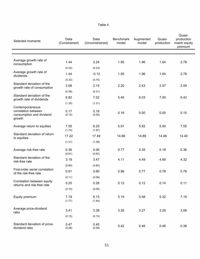
51

Table 4

Selected moments Data (Constrained)

Data (Unconstrained)

Benchmark model

Augmented model

Quasi-production

Quasi-production

match equity premium

Average growth rate of consumption 1.44 2.24 1.95 1.96 1.64 2.78

(0.32) (0.23) Average growth rate of dividends 1.44 -0.12 1.95 1.96 1.64 2.78

(0.32) (0.75) Standard deviation of the growth rate of consumption 2.08 2.15 2.20 2.43 2.57 2.09

(0.38) (0.31) Standard deviation of the growth rate of dividends 6.82 7.02 5.40 6.03 7.00 6.42

(1.35) (1.31) Contemporaneous correlation between consumption and dividend growth

0.17 (0.12)

0.16 (0.09) 0.16 0.00 0.00 0.15

Average return to equities 7.55 6.20 5.91 5.92 5.50 7.55 (1.74) (1.87) Standard deviation of return to equities 17.22 17.49 14.66 14.89 14.48 14.40

(1.31) (1.39) Average risk-free rate 0.36 0.06 0.77 0.35 0.18 0.36 (0.81) (0.83) Standard deviation of the risk-free rate 3.19 3.47 4.11 4.49 4.69 4.32

(0.80) (0.80) First-order serial correlation of the risk-free rate 0.61 0.60 0.96 0.77 0.78 0.78

(0.11) (0.08) Correlation between equity returns and risk-free rate 0.20 0.26 0.12 0.12 0.14 0.11

(0.10) (0.09) Equity premium 7.19 6.13 5.15 5.58 5.32 7.19 (1.77) (1.84) Average price-dividend ratio 3.41 3.38 3.26 3.27 3.29 3.08

(0.15) (0.15) Standard deviation of price-dividend ratio

0.47 (0.08)

0.45 (0.08) 0.42 0.46 0.46 0.38

52

Table 5: Equity and Valuation Risk Premiums

Benchmark Model Augmented Model Quasi-production model

ρ Equity

premium

Conventio- nal Risk

Premium

Valuation Risk

Premium ρ

Equity premium

Conventio- nal Risk

Premium

Valuation Risk

Premium ρ

Equity premium

Conventio- nal Risk

Premium

Valuation Risk

Premium

0.000 -0.0013 -0.0013 0.0000 0.000 -0.0007 -0.0007 0.0000 0.000 -0.0013 -0.0013 0.0000 0.100 -0.0013 -0.0013 0.0000 0.100 -0.0007 -0.0007 0.0000 0.100 -0.0014 -0.0014 0.0000 0.300 -0.0013 -0.0013 0.0000 0.300 -0.0007 -0.0007 0.0000 0.300 -0.0014 -0.0014 0.0000 0.500 -0.0012 -0.0012 0.0000 0.500 -0.0007 -0.0007 0.0000 0.500 -0.0014 -0.0014 0.0000 0.700 -0.0012 -0.0012 0.0000 0.700 -0.0006 -0.0006 0.0000 0.700 -0.0014 -0.0014 0.0000 0.900 -0.0009 -0.0013 0.0004 0.900 -0.0003 -0.0006 0.0003 0.900 -0.0014 -0.0018 0.0004 0.950 0.0003 -0.0012 0.0015 0.950 0.0007 -0.0006 0.0013 0.950 -0.0007 -0.0023 0.0016 0.960 0.0011 -0.0012 0.0023 0.960 0.0014 -0.0007 0.0021 0.960 0.0000 -0.0025 0.0025 0.970 0.0028 -0.0012 0.0040 0.970 0.0029 -0.0007 0.0036 0.970 0.0014 -0.0029 0.0043 0.980 0.0072 -0.0012 0.0084 0.980 0.0069 -0.0006 0.0075 0.980 0.0054 -0.0036 0.0090 0.990 0.0248 -0.0012 0.0260 0.990 0.0230 -0.0007 0.0237 0.990 0.0225 -0.0053 0.0278 0.991 0.0288 -0.0012 0.0300 0.991 0.0268 -0.0006 0.0274 0.991 0.0265 -0.0055 0.0320 0.992 0.0336 -0.0013 0.0349 0.992 0.0313 -0.0007 0.0320 0.992 0.0313 -0.0059 0.0372 0.993 0.0395 -0.0012 0.0407 0.993 0.0369 -0.0007 0.0376 0.993 0.0372 -0.0062 0.0434 0.994 0.0465 -0.0013 0.0478 0.994 0.0436 -0.0007 0.0443 0.994 0.0442 -0.0067 0.0509 0.995 0.0549 -0.0013 0.0562 0.995 0.0517 -0.0007 0.0524 0.995 0.0527 -0.0070 0.0597 0.996 0.0649 -0.0012 0.0661 0.996 0.0613 -0.0007 0.0620 0.996 0.0626 -0.0076 0.0702 0.997 0.0765 -0.0012 0.0777 0.997 0.0726 -0.0007 0.0733 0.997 0.0742 -0.0081 0.0823 0.998 0.0898 -0.0013 0.0911 0.998 0.0857 -0.0007 0.0864 0.998 0.0875 -0.0086 0.0961 0.999 0.1049 -0.0012 0.1061 0.999 0.1006 -0.0007 0.1013 0.999 0.1025 -0.0091 0.1116

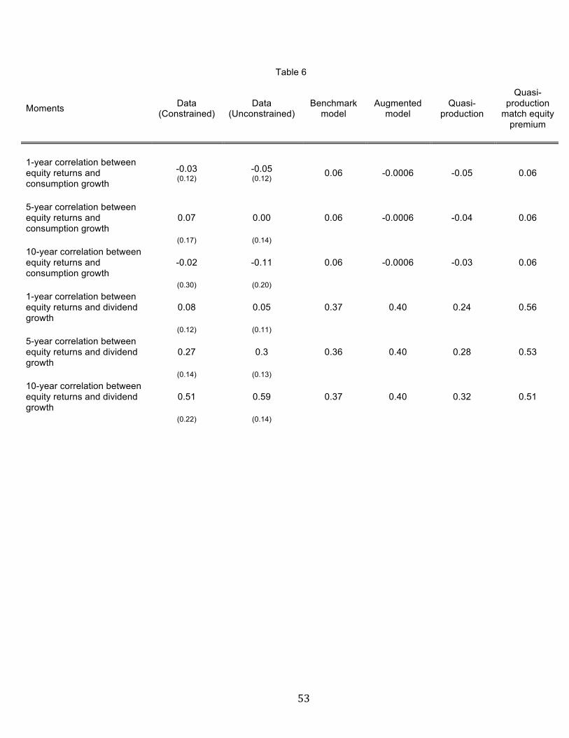
53

Table 6

Moments Data (Constrained)

Data (Unconstrained)

Benchmark model

Augmented model

Quasi-production

Quasi-production

match equity premium

1-year correlation between equity returns and consumption growth

-0.03 (0.12)

-0.05 (0.12) 0.06 -0.0006 -0.05 0.06

5-year correlation between equity returns and consumption growth

0.07 0.00 0.06 -0.0006 -0.04 0.06

(0.17) (0.14) 10-year correlation between equity returns and consumption growth

-0.02 -0.11 0.06 -0.0006 -0.03 0.06

(0.30) (0.20) 1-year correlation between equity returns and dividend growth

0.08 0.05 0.37 0.40 0.24 0.56

(0.12) (0.11) 5-year correlation between equity returns and dividend growth

0.27 0.3 0.36 0.40 0.28 0.53

(0.14) (0.13) 10-year correlation between equity returns and dividend growth

0.51 0.59 0.37 0.40 0.32 0.51

(0.22) (0.14)

54

Table 7

Moments Data (Unconstrained)

Benchmark model

Augmented model

Quasi-production

model

Average yield Long-term bond 1.66 4.60 4.38 4.53 (0.85) Intermediate-term bond 1.06 2.16 1.81 1.79 (0.90) Short-term bond 0.36 0.77 0.35 0.18 (0.81) Return to equity minus long-term bond yield 4.54 1.62 2.02 1.25 (1.84) Standard deviation Long-term bond 3.54 2.32 2.43 2.45 (0.76) Intermediate-term bond 3.65 3.53 3.5 3.36 (0.82) Short-term bond 3.20 4.11 4.49 4.69 (0.80) Return to equity minus long-term bond yield 16.7 14.41 14.64 14.42 (1.48)

55

Table 8

Predictability of excess returns

Data

Price/Dividend Price/Consumption Price/Trend Price/Dividend Price/Consumption Price/Trend Slope R-square 1 year -0.09 -0.17 -0.24 0.04 0.11 0.17 (0.03) (0.06) (0.09) 3 years -0.26 -0.37 -0.49 0.13 0.20 0.29 (0.07) (0.012) (0.14) 5 years -0.39 -0.49 -0.55 0.23 0.27 0.29 (0.11) (0.14) (0.15)

Model (median) Price/Dividend Price/Consumption Price/Trend Price/Dividend Price/Consumption Price/Trend Slope R-square* 1 year -0.04 -0.04 -0.04 0.01 0.01 0.01 (0.06) (0.06) (0.05) 13.1% 0.9% 0.0% 3 years -0.12 -0.12 -0.11 0.03 0.03 0.04 (0.16) (0.15) (0.13) 9.8% 4.3% 0.9% 5 years -0.20 -0.20 -0.19 0.05 0.06 0.06 (0.24) (0.23) (0.21) 7.1% 6.5% 5.9%

Notes: Excess returns over holding periods of 1, 3, and 5 years are regressed on lagged RHS variables Price-dividend ratio, price-consumption ratio, and price-trend ratio. Slope coefficient for each of the regressions is reported as well as the R-square of the regressions. Regressions are estimated with US data and simulated data from the quasi-production model economy. (*) The number underneath the median R-squared is the fraction of simulations that yield an R-square that is at least as large as the sample R-square.