Hydraulics Tutorial - Energy Dissipation in a Drop-Structure Flow

Problem Description & Objectives The flow of water over a vertical drop structure will be simulated where the only known flow characteristic is the upstream depth. The purpose of this exercise is to determine and validate the energy loss of the flow over the drop. To do this, we will simulate the problem and use the results to identify:

the volumetric flow rate over the drop the location, depth, and velocity of critical flow without assuming an a priori flow regime the depth and length of the drop pool the downstream depth of flow the energy loss of the flow over the drop, and empirical results in the literature, compared to the model results for validation

It would be much easier to determine the objectives if the flow rate was known already; it makes a better learning problem to assume only an upstream depth.

FLOW-3D Learning Objectives In this exercise we will learn techniques to:

create the drop structure geometry create the computational domain specify appropriate boundary conditions input fluid properties activate required physical models run the simulation analyze the simulation results compute drop characteristics from results

Figure 1: Rectangular vertical drop structure

Problem Specification Unit System

Simulation units – SI

Geometry Specifications

Drop height: 0.62 m Drop length upstream of the brink: 0.7 m Channel length downstream of the brink: 2.0 m

Flow Conditions

Upstream flow depth = 0.24 m Fluid Properties (Water) Viscosity = 0.001 Pa-s Density = 1000 kg/m3

Simulation Specifications

2D in x and z Free surface with sharp interface Incompressible fluid

Create Workspace and Simulation File Open the FLOW-3D interface by double-clicking the FLOW-3D icon on your desktop.

Create a new workspace

Select the Navigator tab from the tab menu at the top of the screen. Select File and New Workspace. Enter "Energy Dissipater Simulations" in the workspace.

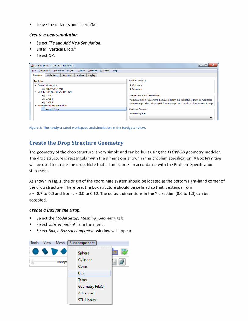
Leave the defaults and select OK.

Create a new simulation

Select File and Add New Simulation. Enter "Vertical Drop." Select OK.

Figure 2: The newly created workspace and simulation in the Navigator view.

Create the Drop Structure Geometry The geometry of the drop structure is very simple and can be built using the FLOW-3D geometry modeler. The drop structure is rectangular with the dimensions shown in the problem specification. A Box Primitive will be used to create the drop. Note that all units are SI in accordance with the Problem Specification statement.

As shown in Fig. 1, the origin of the coordinate system should be located at the bottom right-hand corner of the drop structure. Therefore, the box structure should be defined so that it extends from x = -0.7 to 0.0 and from z = 0.0 to 0.62. The default dimensions in the Y direction (0.0 to 1.0) can be accepted.

Create a Box for the Drop.

Select the Model Setup, Meshing_Geometry tab. Select subcomponent from the menu. Select Box, a Box subcomponent window will appear.

Figure 3: Use Box Primitive to create the drop structure

Enter X, Y and Z dimensions of the geometry as shown in Fig. 4 below.

Figure 4: Dimensions of the geometry

Click OK. The box is a solid, so select Standard as the Component Type. Name the component Drop, like the subcomponent, and click OK.

You should now see a cube in the Meshing and Geometry windows as shown in Fig. 5. This block is the drop structure. A mesh block will be added in the next step to specify the computational domain.

Figure 5: Dimensions of the geometry

Specify the Computational Domain (Mesh) Limits At this point the geometry of the drop structure is specified and the next step is to specify the computational domain and apply a mesh to it. A computational mesh will be added so that it encompasses the drop structure and also extends downstream 2.0 m from the end of the drop. The upstream and downstream flow characteristics will be represented by mesh boundaries. Since the cross-stream flow variations are negligible, a 2-D mesh with one cell and unit length (1.0 m) in the Y direction is appropriate.

According to the sketch in Fig. 1, the computational domain should be defined from x =-0.7 m to x = 2.0 m. The decision on how far upstream and downstream the computational domain should extend from the brink is based on two criteria:

Minimize the size of the computational domain to avoid unnecessary computations. Do not minimize the size of the computational domain to the point where the boundary conditions are

too close to regions of high flow gradients as this can affect the results.

In the Model Setup > Meshing and Geometry tab, add a mesh block by right-clicking on Mesh – Cartesian and selecting Add a mesh block.

Change the definitions of Fixed Pt.s (1) and (2) (the mesh boundaries) to -0.7 and 2.0, respectively, so the mesh is defined as shown in Fig. 6. Name the block 2-D Domain.

Figure 6: Default mesh block included in all simulations

RULE OF THUMB: PLACING ADDITIONAL FIXED POINTS IN REGIONS OF THE COMPUTATIONAL DOMAIN WHERE

SOLID/FLUID FLOW INTERFACES OCCUR OFTEN PRODUCES BETTER MODEL RESULTS. ALSO, FIXED POINTS CAN BE USEFUL

FOR RESOLVING SOLID SURFACES MORE ACCURATELY WITHOUT USING AN UNNECESSARILY FINE MESH FOR THE ENTIRE

PROBLEM. IT IS RECOMMENDED THAT FIXED POINTS BE SPECIFIED ALONG FLAT SURFACES OF GEOMETRY, BUT NEVER

ALONG FREE SURFACES OF FLUID.

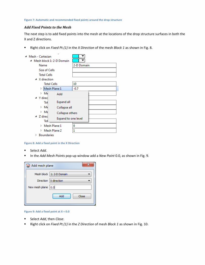
Figure 7: Automatic and recommended fixed points around the drop structure

Add Fixed Points to the Mesh

The next step is to add fixed points into the mesh at the locations of the drop structure surfaces in both the X and Z directions.

Right click on Fixed Pt.(1) in the X Direction of the mesh Block 1 as shown in Fig. 8.

Figure 8: Add a fixed point in the X Direction

Select Add. In the Add Mesh Points pop-up window add a New Point 0.0, as shown in Fig. 9.

Figure 9: Add a fixed point at X = 0.0

Select Add, then Close. Right click on Fixed Pt.(1) in the Z Direction of mesh Block 1 as shown in Fig. 10.

Figure 10: Add a fixed point in the Z Direction

Select Add. In the Add Mesh Points pop-up window, add a New Point 0.62 in the Z Direction, as shown in Fig. 11.

Figure 11: Add a fixed point at Z = 0.62

Select Add, then Close. Save your work.

Resolving Flow Features The choice of mesh cell size is an important one. The computational mesh should be only fine enough to resolve the geometry and capture the flow features of interest. An excessively fine mesh will needlessly increase the simulation runtime and may require more hardware (memory, video).

Without knowing the flow characteristics beforehand, it can be difficult to specify the mesh resolution with great precision. One solution is to run the simulation several times with decreasing mesh resolutions until no significant change in results is observed. A better approach, when possible, is to determine the critical flow feature using general characteristics such as flow depth or rate, and select the necessary mesh size to resolve it. If it is noticed after running the simulation that some flow features are still not well resolved, the simulation can be re-run or restarted with a smaller mesh resolution. Restarting simulations at a midway point in the run will be covered as a later topic in this class.

RULE OF THUMB: A RULE OF THUMB FOR MESH RESOLUTION IS THAT AT LEAST 3 CELLS ARE REQUIRED TO RESOLVE A

FLOW FEATURE SUCH AS A FREE-SURFACE JET.

Figure 12: Critical Flow Feature to Determine Optimal Mesh Size.

In order to follow the rule of thumb, we need to determine the size of the cells necessary to adequately resolve the free-surface jet. To do that we need to determine the minimum thickness of the nappe. As the water flows over the drop and forms the nappe, it accelerates under gravity and becomes thinner, so the minimum thickness occurs at the impact between the nappe and the receiving pool, as shown in Fig. 12.Let's estimate the thickness of the nappe:

Empirical relations by Rand (1955) will be used to estimate the nappe thickness dnappe at the pool impact. The depth of the flow at the inlet (Hupstream) = 0.24 m as defined in the Problem Specification, above.

From Rand (1955), .

Critical flow depth for a rectangular channel is defined as .

The upstream discharge per unit width (qW) is unknown, so we must take intermediate steps to determine the flow rate. This simulation runs quickly, so we will run the simulation with an assumed (coarse) mesh size and use a feature of FLOW-3D called Probe along with a set of generated simulation data called Mesh Dependent History to determine the volumetric flow rate. Before we can run the simulation, we need to define the boundary conditions and fluid properties, as well as physical parameters like gravity.

Specify Boundary Conditions Boundaries conditions define what happens at the edges of the mesh. They can be used to add fluid to the boundary over time, act as sinks for the fluid, maintain pressure, act as walls, and for other functions.

A Pressure boundary condition with specified fluid height will be specified at the upstream (minimum X) boundary since the depth of the flow is known there. Downstream conditions are not known except for the fact that the flow leaves the computational domain at the maximum X boundary so we will use outflow boundary condition downstream.

Specify a Pressure Boundary Condition

A pressure boundary condition with a fluid depth needs to be specified at the X-minimum boundary (the upstream boundary).

Select the Model Setup > Meshing & Geometry > Mesh – Cartesian > Mesh Block 1 > Boundaries tree, and then select the X-min boundary by expanding the tree at the left. The dialog box shown in Fig. 13 will appear.

Select the Specified pressure radio button. Enter 0.86 in the Fluid height box. (Fluid depth upstream is 0.24m and height of the drop is 0.62m from

the x-axis so the Fluid height, in the Z coordinate, = 0.24 + 0.62 = 0.86 m). Keep the Pressure box entry blank which means a value of zero will be used as reference to set

hydrostatic pressure at the boundary. Set F Fraction = 1.0 (all fluid entering the simulation is 100% water) and leave Stagnation Pressure active (flow enters at zero velocity, as from a reservoir. This means that steady-state flow velocity is computed within the mesh, which will give the most accurate result, assuming the boundary is far enough away from the drop structure edge).

Click OK.

Figure 13: Pressure boundary condition

Specify Outflow Boundary Condition

An outflow boundary condition will be specified at X-maximum boundary (the downstream boundary). Fluid is permitted to leave the boundary, but not to enter. This option assumes that the flow through the boundary is super-critical (Froude number greater than 1).

Select the X-max boundary. Select the Outflow radio button. Click OK.

Set Wall Boundary Condition

Boundary condition at Z-minimum boundary (the downstream channel bottom) to be set to Wall boundary condition. For this problem, friction losses from the channel bottom are assumed to be negligible, so no roughness will be assigned to the wall boundary.

Select the Boundaries tab and then select the Z-min boundary. Select the Wall radio button.

Click OK. Save your work.

Symmetry Boundary Conditions

The remaining boundaries are pre-set as Symmetry boundary conditions. This means that the boundaries will be treated as if conditions outside of the boundary were identical to conditions inside the boundary. For the Y boundaries, this implies that the drop structure is much wider than the mesh. For the Z-maximum boundary, the void above the flow extends infinitely. If the model were poorly designed and flow reached the Z-maximum boundary, it would be reflect downward unphysically.

Specify Fluid Properties From the Problem Specification in the beginning of the exercise, the working fluid in the simulation is water. The viscosity is 0.001 Pa-s and the density is 1000 Kg/m3. The properties can either be entered manually or loaded from the materials database. The properties will be loaded from the materials database for demonstration purposes.

Add Fluid Properties

Select the Model Setup > Fluids tab. From the menu bar at the top of the screen, select Materials > Fluids Database. In the Fluid database under Material Name select Water at 293 K with SI units. Select the Load Fluid 1 button, and then select Convert units to SI (this sets the simulation to SI units,

which can also be set on the General tab). Properties for water in SI system will be loaded. Expand the Properties tree as shown in Fig. 14. Verify that the values for viscosity and density have been

loaded. Note that the viscosity values are grayed out, because we have not activated viscous flow on the Physics tab.

Save your work.

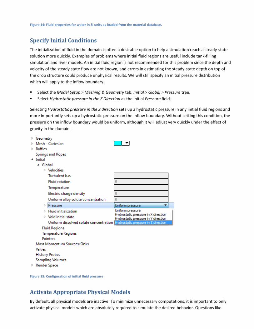
Figure 14: Fluid properties for water in SI units as loaded from the material database.

Specify Initial Conditions The initialization of fluid in the domain is often a desirable option to help a simulation reach a steady-state solution more quickly. Examples of problems where initial fluid regions are useful include tank-filling simulation and river models. An initial fluid region is not recommended for this problem since the depth and velocity of the steady state flow are not known, and errors in estimating the steady-state depth on top of the drop structure could produce unphysical results. We will still specify an initial pressure distribution which will apply to the inflow boundary.

Select the Model Setup > Meshing & Geometry tab, Initial > Global > Pressure tree. Select Hydrostatic pressure in the Z Direction as the initial Pressure field.

Selecting Hydrostatic pressure in the Z direction sets up a hydrostatic pressure in any initial fluid regions and more importantly sets up a hydrostatic pressure on the inflow boundary. Without setting this condition, the pressure on the inflow boundary would be uniform, although it will adjust very quickly under the effect of gravity in the domain.

Figure 15: Configuration of initial fluid pressure

Activate Appropriate Physical Models By default, all physical models are inactive. To minimize unnecessary computations, it is important to only activate physical models which are absolutely required to simulate the desired behavior. Questions like

“Should I treat the simulation is inviscid?” and “Do I need to model surface tension effects?” should be answered early in the modeling process.

The flow below the drop structure is likely highly turbulent so the flow will be modeled as Turbulent with Newtonian viscosity. The only other model which needs to be activated is Gravity. Surface tension effects are insignificant due to the size of the problem, so the Surface Tension model can be left inactive. This can

be demonstrated by calculating the Weber number ( 2We V L / sρ= )where ρ is the fluid density, V is a

characteristic velocity, L is a length scale, and σ is the surface tension coefficient. If We >> 1, surface tension effects can be ignored. Since we do not know the velocity yet, we will have to make a safe assumption that surface tension does not contribute significantly to the flow effects.

In the next step, the appropriate physical models will be activated.

Activate the Gravity Model

Select the Model Setup > Physics tab. Select the Gravity button. Set the value of Gravity component in the Z Direction to -9.81 as shown below.

Figure 16. Gravity Definition

Click OK.

There are a number of choices for Turbulence models in FLOW-3D. The most robust and widely applicable turbulence model is the RNG (Renormalized Group) model. That model requires a maximum turbulent mixing length, which represents the upper limit of the size of an expected turbulent eddy in the simulation and is used to limit the amount of turbulent energy created by the turbulence models.

RULE OF THUMB: A GOOD ESTIMATE OF THE TURBULENT LENGTH SCALE IS 7% OF THE HYDRAULIC DIAMETER (FLOW

DEPTH) IN A HIGHLY TURBULENT REGION WHICH IS LIKELY TO CONTROL THE FLOW. AN ESTIMATE OF THE MAXIMUM

TURBULENT MIXING LENGTH USED IN FLOW-3D IS 7% - 13% OF THE CONTROLLING DEPTH.

One of the problem objectives for this simulation is to determine the depth of the pool. This depth is just upstream of the point where the nappe impinges on the bottom of the channel. This impingement point is the most turbulent region in the domain and also controls significant flow features. Therefore, the thickness of the nappe could be used to estimate the turbulent length scale. Since we do not know the thickness yet, we will ask FLOW-3D to determine the turbulent length scale for us. Specifying your own turbulent mixing

length scale is sometimes preferable to letting FLOW-3D determine the scale automatically, but it can be difficult to estimate.

Activate Viscosity and Turbulence

Activate Newtonian viscosity and RNG turbulence with dynamically-computed max mixing length. Select the Model Setup > Physics tab. Select the Viscosity and turbulence button. The dialog shown in Fig. 17 will appear. Under the Viscosity options, activate the Viscous flow option. Under Turbulence options, select Renormalized group (RNG) model. Under Maximum turbulent mixing length, activate Dynamically computed. Click OK.

Figure 17: Select the RNG turbulence model and set dynamically computed turbulent length scale.

Specify Simulation Finish Time Although it can be difficult to estimate the time at which steady state is reached, a Finish time always needs to be specified so that the simulation knows when to terminate.

RULE OF THUMB: A REASONABLE MEASURE OF THE TIME FOR A FLUID DYNAMIC SYSTEM TO REACH STEADY STATE IS 10

TO 20 CHARACTERISTIC TIME SCALES. THE CHARACTERISTIC TIME SCALE REPRESENTS THE TIME REQUIRED FOR A FLUID

PACKET TO PASS THROUGH THE SYSTEM. A CHARACTERISTIC VELOCITY IN THE DOMAIN NEEDS TO BE ESTIMATED TO

DETERMINE THE CHARACTERISTIC TIME.

Without experimental or simulation data we can only estimate the characteristic velocity. The velocity of the water falling under gravity though a distance of 0.62 m (drop height) is (2*9.81 m/s2*0.62 m)1/2 = 3.5 m/s. The total length of the domain is 2.7 m, so the characteristic time scale is about 0.77 seconds (2.7 / 3.5) and 20 time scales is then about 15 seconds (0.77 * 20).

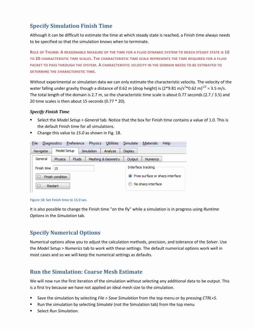
Specify Finish Time

Select the Model Setup > General tab. Notice that the box for Finish time contains a value of 1.0. This is the default Finish time for all simulations.

Change this value to 15.0 as shown in Fig. 18.

Figure 18: Set Finish time to 15.0 sec.

It is also possible to change the Finish time "on the fly" while a simulation is in progress using Runtime Options in the Simulation tab.

Specify Numerical Options Numerical options allow you to adjust the calculation methods, precision, and tolerance of the Solver. Use the Model Setup > Numerics tab to work with these settings. The default numerical options work well in most cases and so we will keep the numerical settings as defaults.

Run the Simulation: Coarse Mesh Estimate We will now run the first iteration of the simulation without selecting any additional data to be output. This is a first try because we have not applied an ideal mesh size to the simulation.

Save the simulation by selecting File > Save Simulation from the top menu or by pressing CTRL+S. Run the simulation by selecting Simulate (not the Simulation tab) from the top menu Select Run Simulation.

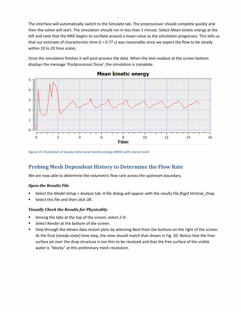
The interface will automatically switch to the Simulate tab. The preprocessor should complete quickly and then the solver will start. The simulation should run in less than 1 minute. Select Mean kinetic energy at the left and note that the MKE begins to oscillate around a mean value as the simulation progresses. This tells us that our estimate of characteristic time (t = 0.77 s) was reasonable since we expect the flow to be steady within 10 to 20 time scales.

Once the simulation finishes it will post-process the data. When the text readout at the screen bottom displays the message 'Postprocessor Done', the simulation is complete.

Figure 19: Oscillation of steady-state mean kinetic energy (MKE) with coarse mesh

Probing Mesh Dependent History to Determine the Flow Rate We are now able to determine the volumetric flow rate across the upstream boundary.

Open the Results File

Select the Model Setup > Analyze tab. A file dialog will appear with the results file flsgrf.Vertical_Drop. Select this file and then click OK.

Visually Check the Results for Physicality

Among the tabs at the top of the screen, select 2-D. Select Render at the bottom of the screen. Step through the eleven data restart plots by selecting Next from the buttons on the right of the screen.

At the final (steady-state) time step, the view should match that shown in Fig. 20. Notice that the free-surface jet over the drop structure is too thin to be resolved and that the free surface of the visible water is “blocky” at this preliminary mesh resolution.

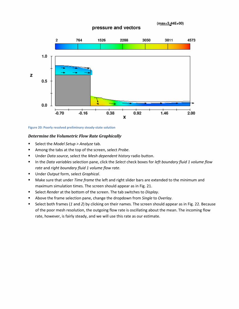
Figure 20: Poorly resolved preliminary steady-state solution

Determine the Volumetric Flow Rate Graphically

Select the Model Setup > Analyze tab. Among the tabs at the top of the screen, select Probe. Under Data source, select the Mesh dependent history radio button. In the Data variables selection pane, click the Select check boxes for left boundary fluid 1 volume flow

rate and right boundary fluid 1 volume flow rate. Under Output form, select Graphical. Make sure that under Time frame the left and right slider bars are extended to the minimum and

maximum simulation times. The screen should appear as in Fig. 21. Select Render at the bottom of the screen. The tab switches to Display. Above the frame selection pane, change the dropdown from Single to Overlay. Select both frames (1 and 2) by clicking on their names. The screen should appear as in Fig. 22. Because

of the poor mesh resolution, the outgoing flow rate is oscillating about the mean. The incoming flow rate, however, is fairly steady, and we will use this rate as our estimate.

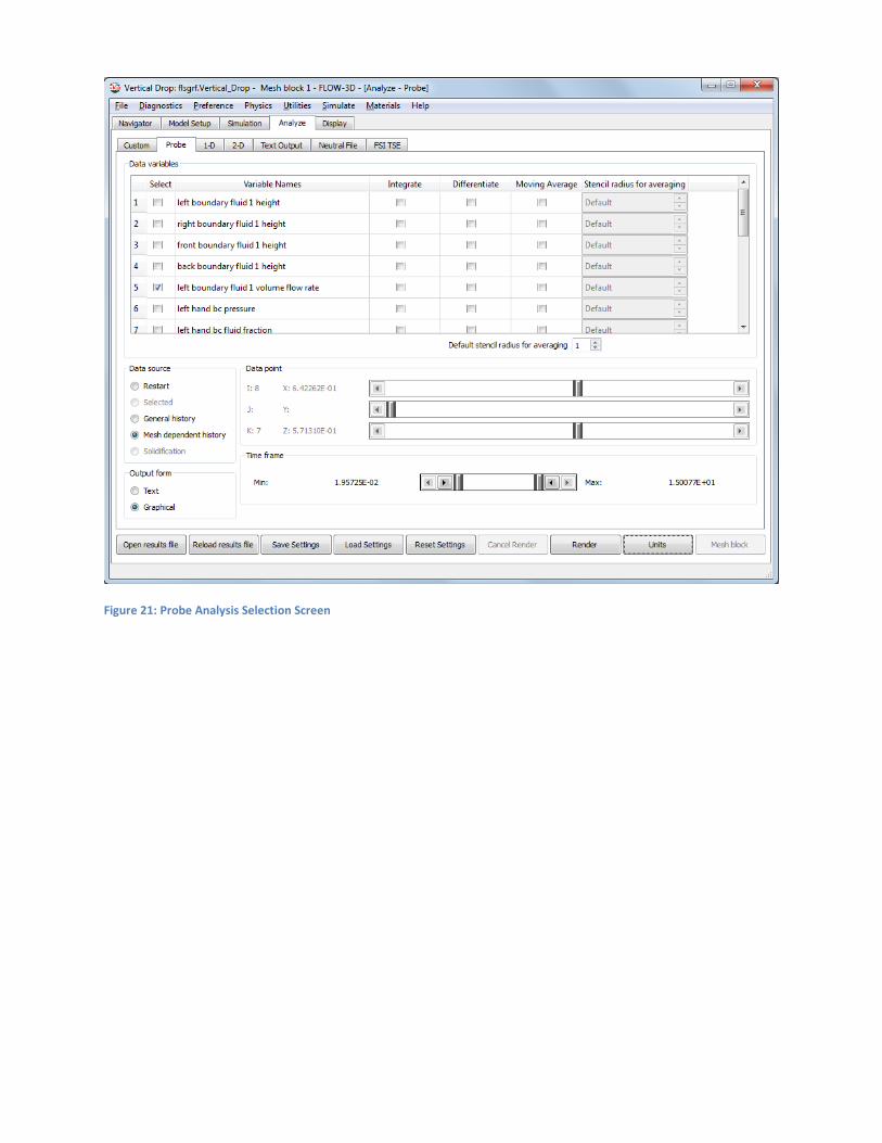
Figure 21: Probe Analysis Selection Screen

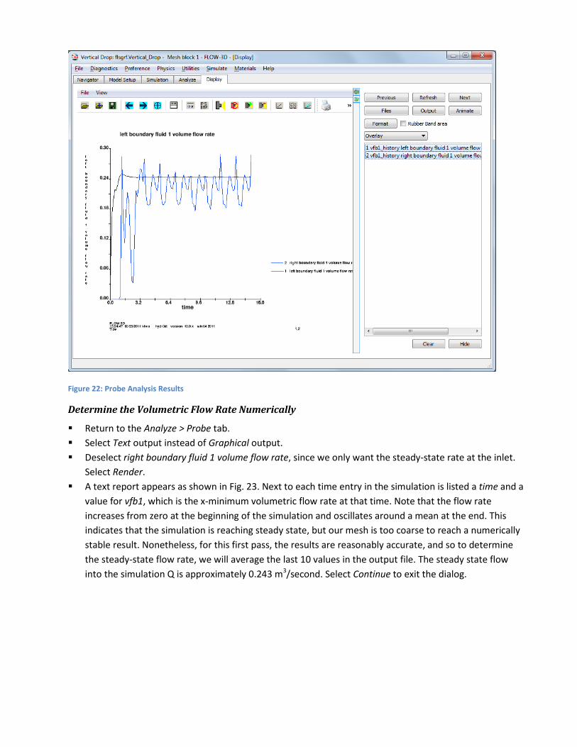
Figure 22: Probe Analysis Results

Determine the Volumetric Flow Rate Numerically

Return to the Analyze > Probe tab. Select Text output instead of Graphical output. Deselect right boundary fluid 1 volume flow rate, since we only want the steady-state rate at the inlet.

Select Render. A text report appears as shown in Fig. 23. Next to each time entry in the simulation is listed a time and a

value for vfb1, which is the x-minimum volumetric flow rate at that time. Note that the flow rate increases from zero at the beginning of the simulation and oscillates around a mean at the end. This indicates that the simulation is reaching steady state, but our mesh is too coarse to reach a numerically stable result. Nonetheless, for this first pass, the results are reasonably accurate, and so to determine the steady-state flow rate, we will average the last 10 values in the output file. The steady state flow into the simulation Q is approximately 0.243 m3/second. Select Continue to exit the dialog.

Figure 23: Text Output of Volumetric Flow Rate

Using the Coarse Flow Rate to Estimate the Nappe Width Now we are ready to adjust the mesh to the minimum necessary to resolve our problem. First, we return to the equations of Rand (1955) to estimate the nappe width.

From Rand (1955), .

The drop height Hdrop = 0.62 meters as defined in the Problem Specification, above.

Critical flow depth for a rectangular channel is defined as .

qW is the flow rate per unit width. Since our simulation is 1 meter wide (the mesh extents in the y-coordinate are 0,1), qW = 0.243 m2/s.

Gravity was previously defined on the Physics tab as g = 9.81 m/s2 in the downward direction.

We can estimate the thickness of the nappe is about 0.069 m. Therefore, a mesh size of 0.069/3 = 0.023 m is probably adequate to resolve the flow. Rounding down, we will use a mesh resolution of 0.02 m.

Refine the Mesh Using the Nappe Width

Refine the Mesh to Resolve the Flow at the Nappe.

Select the Model Setup > Meshing and Geometry tab. Expand the Mesh - Cartesian > Mesh Block 1 tree at the left. Right click on Mesh Block 1 (as shown in Fig. 23) and select Auto mesh.

Figure 23: Use Auto Mesh to generate mesh cells

In the Auto Mesh pop-up window select X Direction and Z Direction. Select Size of Cells and enter the cell lengths as 0.02.

Figure 24: Specify a cell size of 0.02 m in the X and Z Directions

Click OK. Save your work.

Apply a Constant Maximum Turbulent Mixing Length As previously discussed, it is usually more appropriate to use a dynamically calculated maximum turbulent mixing length. This is somewhat a matter of taste and experience, and there are situations (like sediment scour simulations) where a manually selected length is more effective. We will now select a manual length for demonstration purposes. Normally this step would only be applied if there was a problem with the turbulence modeling.

The nappe was estimated to have a thickness of 0.07 m, and the depth of the flow in the impingement region is probably about twice the nappe thickness (this is a rough estimate). This gives an estimate of the turbulent length scale of 2 * 0.07 m * 7% = 0.0098 m.

Change the Turbulent Mixing Length Method

Select the Model Setup > Physics tab. Select the Viscosity and turbulence button. The dialog shown in Fig. 25 will appear. Under Maximum turbulent mixing length, change the method to select Constant, and enter 0.0098 as

the constant turbulent mixing length. Click OK.

Figure 25: Switch to a manually calculated turbulent length scale.

Add Flux Surfaces to Analysis We are interested in the depth of flow db at the edge of the drop. Because the edge of the drop is a precise location we would rather not use a cell-centered average value. We will use a flux surface to find the flow depth directly. Flux surfaces, also called flux planes, are a diagnostic feature in FLOW-3D for recording time-dependent fluid and energy flow rates and other hydraulic parameters as well as counting particles and scalar concentrations. Although they can have any porosity, flux surfaces that are used as sampling points are represented as 100% porous baffles so they do not affect the flow in any way.

Set up a Flux Surface at the Drop Edge.

Select the Model Setup > Meshing & Geometry tab. Since the edge of the drop structure is at x = -0.0, we will place our first flux surface there. Note that

baffles, including flux surfaces, occur by definition at the interface between cell planes. Because of this constraint, flux surfaces will be moved during pre-processing to the nearest cell face, and this means that baffles that are slanted relative to the mesh will become stepped.

In the meshing tree on the left, right-click Baffles, and select Add. Expand the newly added Baffle 1 tree and activate Define as Flux Surface. Expand the Definitions portion of the Baffle 1 > Baffle Region 1 tree and enter 0.0 as the X Coordinate.

This creates a flux plane across the entire Y-Z plane at x = 0. Note that we could also use the Limiters portion of the tree to create a flux surface that is like a window within the mesh.

Expand the Porosity Properties for Baffle 1 and set Porosity to 1.0. Give the Baffle Name as Edge and Save your work. The tree should appear as in Fig. 26.

Figure 26: Adding a Flux Plane Baffle

Check your work using FAVORize. FAVORize is a tool that allows you to see your geometry and initial fluid regions the way the FLOW-3D solver will see it. It is a useful tool for checking the resolution of meshes, as well as data that is not visible in the normal Meshing & Geometry view, such as the location

of baffles and initialized fluid. Select the FAVORize button above the display; it looks like this: . Use the radio buttons to View Component Volume as Solid. Select Render.

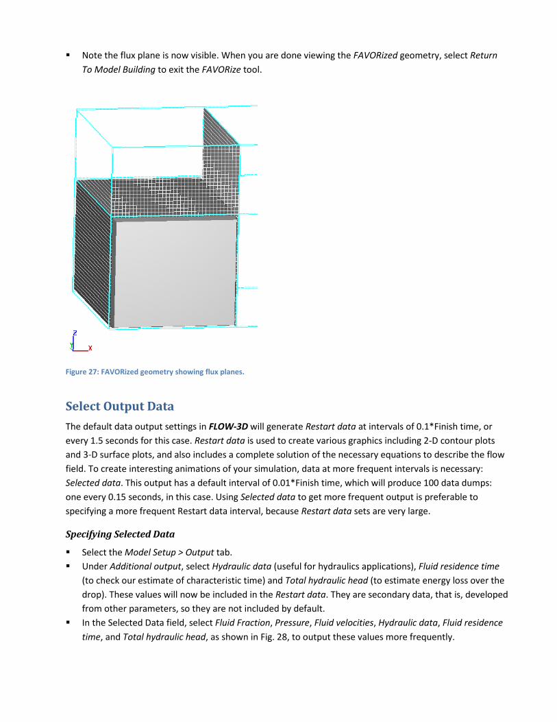
Note the flux plane is now visible. When you are done viewing the FAVORized geometry, select Return To Model Building to exit the FAVORize tool.

Figure 27: FAVORized geometry showing flux planes.

Select Output Data The default data output settings in FLOW-3D will generate Restart data at intervals of 0.1*Finish time, or every 1.5 seconds for this case. Restart data is used to create various graphics including 2-D contour plots and 3-D surface plots, and also includes a complete solution of the necessary equations to describe the flow field. To create interesting animations of your simulation, data at more frequent intervals is necessary: Selected data. This output has a default interval of 0.01*Finish time, which will produce 100 data dumps: one every 0.15 seconds, in this case. Using Selected data to get more frequent output is preferable to specifying a more frequent Restart data interval, because Restart data sets are very large.

Specifying Selected Data

Select the Model Setup > Output tab. Under Additional output, select Hydraulic data (useful for hydraulics applications), Fluid residence time

(to check our estimate of characteristic time) and Total hydraulic head (to estimate energy loss over the drop). These values will now be included in the Restart data. They are secondary data, that is, developed from other parameters, so they are not included by default.

In the Selected Data field, select Fluid Fraction, Pressure, Fluid velocities, Hydraulic data, Fluid residence time, and Total hydraulic head, as shown in Fig. 28, to output these values more frequently.

Figure 28: Choose selected data for output

Throughout the simulation these selected flow quantities will be written out at intervals of 0.01*the Finish time. In this case, Selected data will be written at t = 0.00, 0.15, 0.30, 0.45 ... 15.00 seconds.

Run the Simulation: Refined Mesh We will now run the second iteration of the simulation with our additional output data selected.

Save the new simulation by selecting File > Save Simulation from the top menu or by pressing CTRL+S. Select the menu bar dropdown Simulate (not the Simulation tab) from the top menu bar. Select Run

Simulation. When notified that the output file flsgrf.Vertical_Drop already exists, select Overwrite. Note that if the

goal were to compare the model results with the coarse mesh and the refined mesh, we would want to save the new results file with a different name. The simulation run time will vary depending on many factors: the type and number of processors available and used for the simulation, the number and type of other programs running (including operating system processor use), available memory, hard disk space available, and others.

Select Mean kinetic energy at the left. Note that this time, with the refined mesh, the MKE comes to steady state without oscillating. This is one indicator that our mesh size is reasonable.

Click on the red Warnings and Errors button to get a readout of notable moments in the simulation.

There is one convective flux error at the beginning of the simulation: convective flux iterations (by the explicit solver) do not affect accuracy, and can safely be ignored when they do not cause excessively small time steps, and especially when they occur at the beginning of the simulation.

There is one Mentor Tip that the fluid volume error exceeds 5%. Looking at the output plot on the Simulation tab for Conv. volume error (% lost) shows an erroneous fluid gain of about 14% before the first second of the simulation elapsed. This indicates that mass conservation is negatively affected, and implies an incorrect solution at that time. However, by the beginning of the quasi-

steady state solution at t = 8 seconds, the total error is less than 2% and improves from there, so we have confidence in our results.

There are several Mentor Tips that the flow is nearly steady: these confirm that we selected an adequate Finish time, and let us know that the flow is nearly steady by 8.7 seconds (we will use this later to derive time-averaged values).

Once the simulation finishes it will post-process the data. When the text readout at the screen bottom displays the message 'Postprocessor Done,' the simulation is complete.

Figure 29: No oscillation of steady-state mean kinetic energy (MKE) with resolved mesh

Analyze Simulation Results The ultimate goal of the simulation is to determine the flow characteristics such as flow depths and energy losses. The results of the simulation can be analyzed while the simulation is running or after the simulation has completed.

Open the Results File and Check for Physicality

Select the Analyze tab. Note that the option Reload results file is highlighted in red. Select this to reload the newly overwritten

flsgrf.Vertical_Drop results file. Among the tabs at the top of the screen, select 2-D. Accept the default contour variable (pressure) and

vector type (plain velocity vectors). Select the Vector Options box and a vector spacing of one per every two cells by entering 2 for X and

Z.Select OK to close the dialog. Expand the X Limits Sliders and Z Limits Sliders to display the entire domain. Expand the Time Frame Sliders to cover all available Restart data time steps (t = 0 to t = 15 seconds).

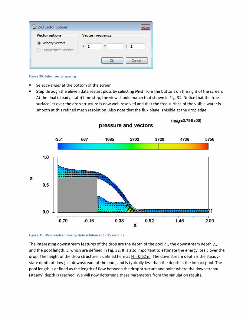
Figure 30: Select vector spacing

Select Render at the bottom of the screen. Step through the eleven data restart plots by selecting Next from the buttons on the right of the screen.

At the final (steady-state) time step, the view should match that shown in Fig. 31. Notice that the free-surface jet over the drop structure is now well-resolved and that the free surface of the visible water is smooth at this refined mesh resolution. Also note that the flux plane is visible at the drop edge.

Figure 31: Well-resolved steady-state solution at t = 15 seconds

The interesting downstream features of the drop are the depth of the pool hp, the downstream depth yp, and the pool length, L, which are defined in Fig. 32. It is also important to estimate the energy loss E over the drop. The height of the drop structure is defined here as H = 0.62 m. The downstream depth is the steady-state depth of flow just downstream of the pool, and is typically less than the depth in the impact pool. The pool length is defined as the length of flow between the drop structure and point where the downstream (steady) depth is reached. We will now determine these parameters from the simulation results.

Figure 32: Characteristics of flow over the drop structure.

Determine Pool Length L

The pool length L is the distance from the drop surface to the point where the angle of the nappe entering the pool coincides with the floor. Because the angle of the nappe varies after entering the pool, it can be difficult to define the location of the downstream end of the pool. We will estimate this point as the point at which the vertical component of velocity approaches zero.

Select the Analyze > Text Output tab. Select Selected as the Data source. This selects the output data that was written every hundredth of the

simulation time (every 0.15 seconds). Select z-velocity in the Data variable list. Select the X Limits sliders to output values for the cells between x = 0.51 m and x = 1.99 m (the locations

listed are the cell centers). Move the Z Limits sliders together to output the component velocity at cell center z = 0.01. Move both sliders in Time frame to the last time frame, t = 15 seconds, as this is the only time frame

we're interested in currently. Click the Render button. The results will appear as shown in Fig. 33 below. The z-magnitude velocity is very negative where the pool entry occurs, quickly leveling out by x = 0.91

m, and then slightly positive as the flow thickens downstream of the nappe. We can interpolate the inflection point where z-velocity = 0 to be the end of the pool at x = L = 0.913 m at the final time step.

We might expect that the location of the inflection point will vary with time, even though the simulation has reached steady state. For many problems, it would be sufficient to use the final time step value as our steady-state estimate. We can check this assumption by moving the X Limits sliders to plot only x = 0.81 to x = 0.97, and extending the Time frame sliders to cover the time period from t = 8.7 seconds to t = 15 seconds (the time period during which the solver reported the flow as nearly steady). Select Render to see the output as shown in Fig. 34.

Copying this data to a spreadsheet program for manipulation allows us to take the time average of the interpolated inflection points to compare to the final time step. This gives a more accurate estimate

than in the previous step, as it shows the oscillation of the pool length due to turbulence. The pool length L varies between 0.841 and 0.938 m, and the average pool length L is 0.883 m.

Figure 33: Text output of Z-Velocity showing inflection point at last time-step

Figure 34: Text output of Z-Velocity showing inflection point varying with time

Determine the Downstream Depth y1

Now that we have determined the location of downstream depth y1 in the x-direction (coinciding with the pool length), we can take a time average of the depth at that location. If we are confident with our spreadsheet approach to analyzing the data, we can continue with that method. If we would like FLOW-3D to interpolate the data for us, we can use a Neutral File. To do this, we must write a transf.in file, which is described in more detail later in this manual.

Select the Navigator tab. If you are using Windows, look on the right under Selected Simulation and right-click the path listed for Simulation Input File. The folder containing the simulation will open with the prepin file for the simulation highlighted. If you are using a version of Linux, navigate to the simulation manually.

Create a text file called transf.in using a text editor. Write the file as shown in Fig. 35. The first three lines are optional title lines, the -1 and 0 lines are required placeholders, and the -0.7 0.0 0.0 line gives the x, y, and z coordinates of the minimum domain boundaries, respectively. After that a single point is given with x, y, z coordinates where we wish to interpolate data. The x point is our average pool length L, the y point is the cell center since it is a 2-D simulation, and the z point is also a cell center, since Fluid Depth output is the same for all z-values at a given x and y. We could list as many points as we are

interested in, and get interpolated output for all of them, but we are only interested in one point currently.

Figure 35: Text output of Z-Velocity showing inflection point varying with time

Note that some operating systems (Windows) will attempt to append .txt to the file name. You must remove the added characters by unselecting Hide Extensions for Known File Types under Folder and Search Options and then renaming the file (see your operating system help for more detail).

Once the file is saved, return to the user interface and select Analyze > Neutral File. Under Data Source choose Selected. In the Data variables window select Fluid Depth and deselect any other variables that are highlighted. Move the X Limits and Z Limits Sliders to cover the entire domain. Move the Time-frame sliders to cover the range of times from t = 8.7 seconds to t = 15.0 seconds, as

before. Click the Render button. As shown in Fig. 36, the output (which is also written to a text file called transf.out in the simulation

folder) follows the same format as the input file, with time, title, and placeholder lines followed by the number of output variables (1), the name of the variables (fldpt), a line with the minimum mesh coordinates for reference, and then a line with the interpolation coordinates and variable value(s).

The depth oscillates less than 2 mm at the average inflection point. Taking the time average of the interpolated values shows the downstream depth y1 varies between 0.0562 and 0.0579 m, and averages 0.0572 m.

Figure 36: Interpolated neutral file output showing fluid depth at average pool end location.

Determine the Pool Depth yp

From Fig. 32 it can be seen that the pool depth yp must be measured at a location where two free surfaces exist in the vertical direction (the flow over the drop structure and the pool below it both have free surfaces). Using fluid depth as an output variable, as we did to find the downstream depth, will not work for the pool depth since the output only indicates the depth of the uppermost fluid surface. Instead, fraction of fluid will be used to locate the lower free surface. We will determine the lowest elevation at which the fluid fraction (per cell) transitions from nearly 100% to nearly 0%. This is the free surface transition. The location h1 is just slightly downstream of the drop face which is located at x = 0.0. A text output of fraction of fluid in the vertical row of cells just downstream of the drop will tell us the location of yp.

Select the Analyze > Text Output tab Move both X sliders in the Limits group box to x = 1.0e-2 (sliders move from cell center to cell center,

and our cell size is 0.02 in the x-direction, so 0.01 is the center of the cell adjacent to the x=0 axis, which is also the face of the drop structure).

Select Fraction of Fluid in the Data variables list and deselect any other variables. We want to look at these values in the first column of cells downstream from the drop structure, which

is 0.62 m high. Slide the Z sliders in the Limits group box to include the z-range from 1.0e-2 to 6.1e-1. Move both Time-frame sliders to the last time frame, 15 sec. By doing this, we will only plot the fluid

fractions in the column of cells adjacent to the drop structure face at the final time step. We are assuming that the pool depth is at steady state at this time. If the pool depth is oscillating, then we

would want to include the time average of the steady-state period of the simulation. The selections should appear as in Fig. 37.

Click Render button. The results will appear as shown in Fig. 38.

Figure 37: Limits for using fraction of fluid to determine pool depth

Figure 38: Locating the pool depth water-air transition

In the displayed results you will see that X, Y and Z points are arranged with Z in ascending order. The fluid fraction is displayed for each cell starting at the bottom of the pool and proceeding to the top, cell by cell. Each z-coordinate corresponds to the center of a cell (rounding shows that the cell centers are spaced every 0.02 m, with the lowest cell center at 0.01 m, following our mesh specifications). In the cell with center z = 0.31, the fluid fraction is 0.671 (67.1%). The cell above this, with center z = 0.33, has a fluid fraction of zero (air), and the cell below this (center z = 0.29) has a fluid fraction of 0.99 (wet), so it is in the cell with center 0.31 that the free surface is found. Interpolating using the cell edges: z = 0.30 + 0.671*(0.32 - 0.30) = 0.3134 gives the precise elevation of the free surface at the final time step.

As an optional step, choose Selected data, select z limits = 0.28 to 0.32 m, open the time sliders to cover the steady-state period from t = 8.7 to 15 seconds to the finish, and take the average of the pool depth using fluid fraction as explained above. This is best accomplished in a spreadsheet, although it is helpful to plot it graphically from the Probe tab as shown in Fig. 39. The pool depth ranges between 0.301 and 0.303, and the average pool depth yp is 0.302 m.

Fluid fraction is greater than 0 and less than 1 (0.627) at this location. This indicates the pool free surface is located 62.7% of the distance between 0.30 and 0.32 m.

I i Z

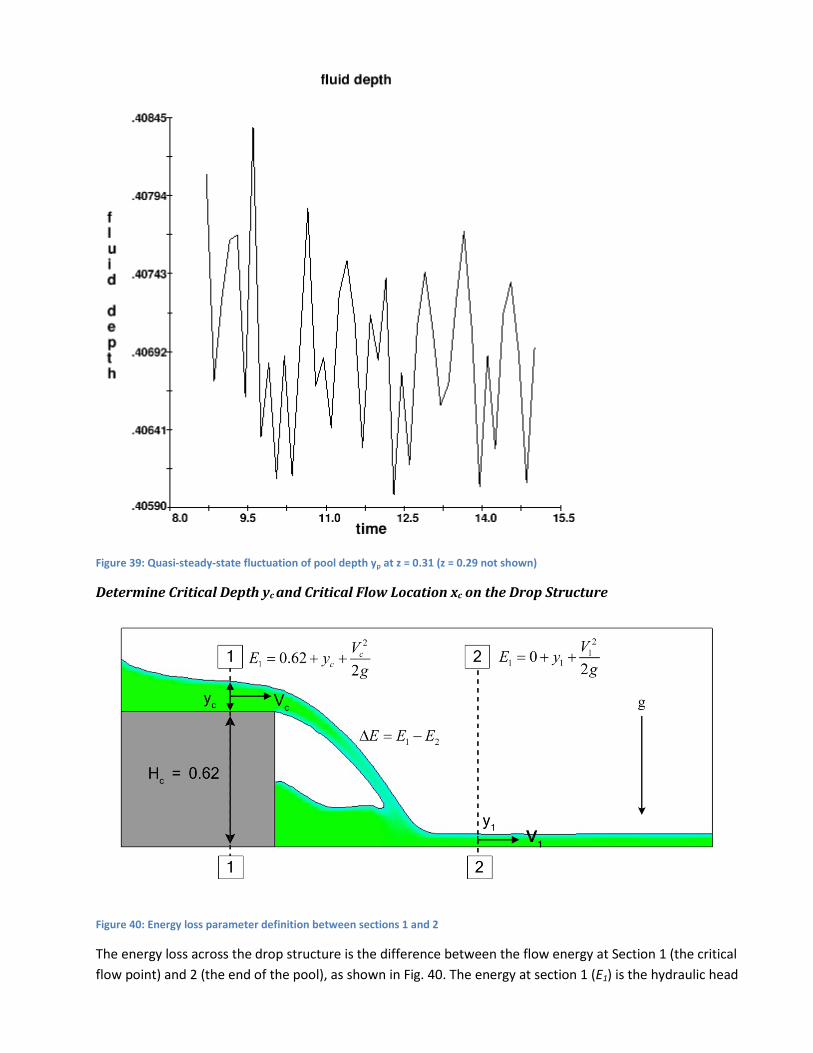
Figure 39: Quasi-steady-state fluctuation of pool depth yp at z = 0.31 (z = 0.29 not shown)

Determine Critical Depth yc and Critical Flow Location xc on the Drop Structure

Figure 40: Energy loss parameter definition between sections 1 and 2

The energy loss across the drop structure is the difference between the flow energy at Section 1 (the critical flow point) and 2 (the end of the pool), as shown in Fig. 40. The energy at section 1 (E1) is the hydraulic head

of the fluid at xc, where subscript c indicates the critical flow section. We will locate the critical flow transition and the hydraulic head of the critical flow point and pool end using FLOW-3D's output.

We must first determine the location xc of the critical transition and the depth yc. The definition of critical flow is flow with Froude number Fr equal to 1, so we need to determine the X location on the drop structure where the Froude number changes from subcritical (Fr < 1.0) to critical (Fr = 1.0). This can be done by creating Text Output of Froude number above the drop structure.

Select the Analyze > Text Output tab. We want to look at Froude number and fluid depth along the X Direction. Choose Selected from the Data

source box on the left. Select (only) Froude Number and Fluid Depth in the Data variable list. Check the sliders in the Limits box: time and z should be maximum only. Fluid depth and Froude number

are reported by FLOW-3D for each column of z-cells, rather than separately for each cell in the column. Using only the top-most z-cell as the reporting criteria prevents repeating the same data over and over for each layer of z-coordinates. The X limit sliders should include the domain from x = -0.69 to x = -0.01 m (upstream of the drop face).

Click Render button. The results will appear as shown in Fig. 41 below.

Figure 41: Identifying critical depth yc

Critical depth can be determined at the point where the Froude number = 1.0. Interpolating the fluid depths and X-direction cell centers between the points where Fr = 0.9975 and 1.0218 in Fig. 39 gives the exact result for the final time step, which if we check does not vary (to four significant digits) during the steady-state period from t = 8.1 to t=15 seconds. The minimum, maximum, and average critical depth yc is 0.1576 m, and occurs at xc = - 0.448 m.

Use the Flux Surface to find Flow Rate Q at the Drop Edge

Select the Analyze > Probe tab, and under Data source select General history (this is where flux surface output is found). In Output form, select Graphical.

In the Data variables window select fluid1 flowrate at Edge. Select Render. The plot will appear as in Fig. 42. To determine the flow rate Q more accurately, re-render the plots in Text mode. Flow rate Q ranges

from 0.1952 to 0.1965 m3/s, with average flow rate Q of 0.1958 m3/s. Note that this differs significantly from our original estimate of 0.243 m3/s, although probably not

significantly enough to warrant recalculating the nappe width and readjusting the turbulent mixing

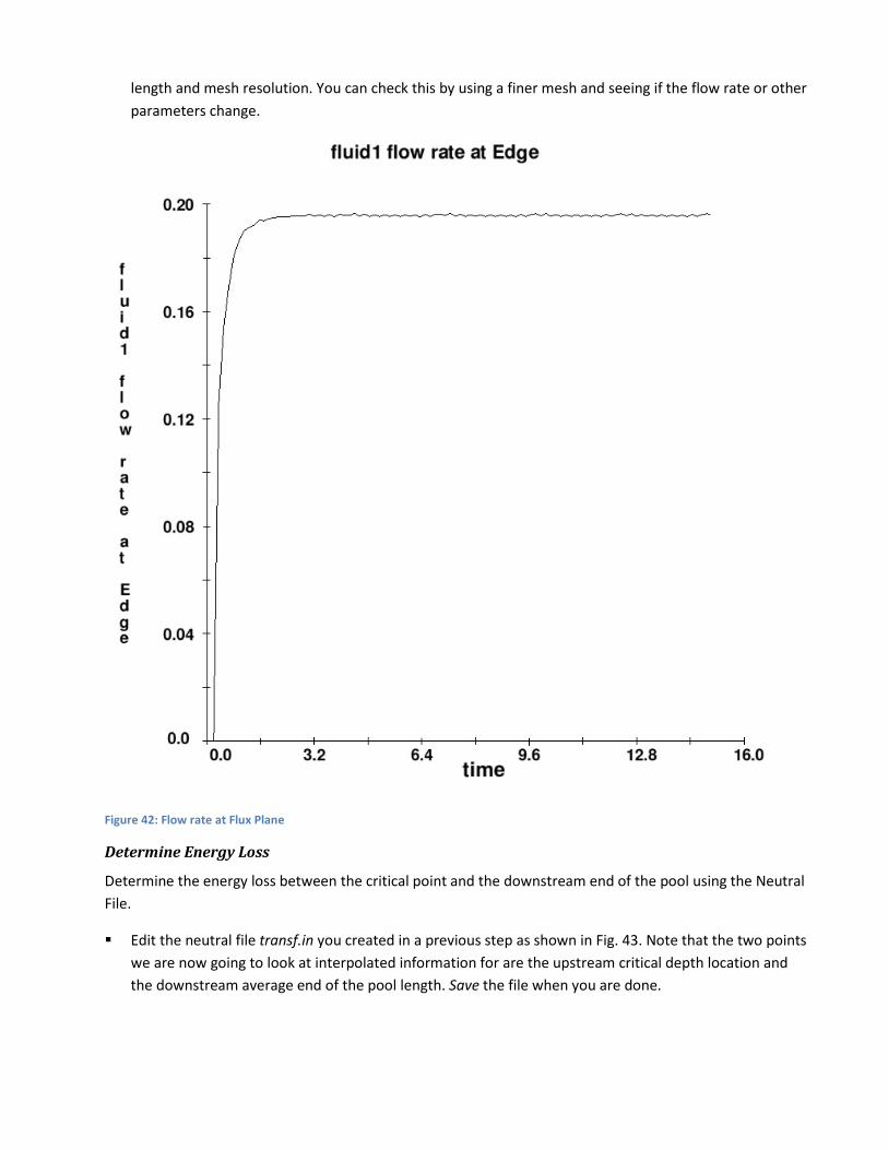
length and mesh resolution. You can check this by using a finer mesh and seeing if the flow rate or other parameters change.

Figure 42: Flow rate at Flux Plane

Determine Energy Loss

Determine the energy loss between the critical point and the downstream end of the pool using the Neutral File.

Edit the neutral file transf.in you created in a previous step as shown in Fig. 43. Note that the two points we are now going to look at interpolated information for are the upstream critical depth location and the downstream average end of the pool length. Save the file when you are done.

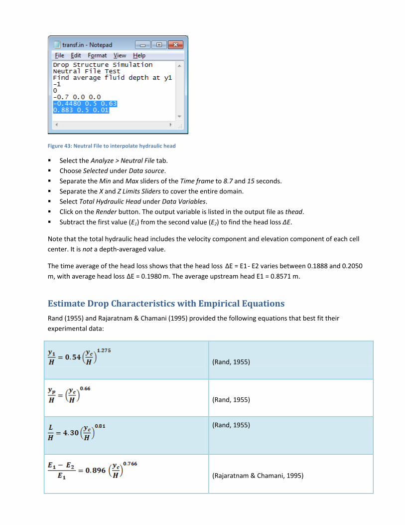
Figure 43: Neutral File to interpolate hydraulic head

Select the Analyze > Neutral File tab. Choose Selected under Data source. Separate the Min and Max sliders of the Time frame to 8.7 and 15 seconds. Separate the X and Z Limits Sliders to cover the entire domain. Select Total Hydraulic Head under Data Variables. Click on the Render button. The output variable is listed in the output file as thead. Subtract the first value (E1) from the second value (E2) to find the head loss ∆E.

Note that the total hydraulic head includes the velocity component and elevation component of each cell center. It is not a depth-averaged value.

The time average of the head loss shows that the head loss ∆E = E1 - E2 varies between 0.1888 and 0.2050 m, with average head loss ∆E = 0.1980 m. The average upstream head E1 = 0.8571 m.

Estimate Drop Characteristics with Empirical Equations Rand (1955) and Rajaratnam & Chamani (1995) provided the following equations that best fit their experimental data:

(Rand, 1955)

(Rand, 1955)

(Rand, 1955)

(Rajaratnam & Chamani, 1995)

Where h1 = pool depth, h2 = downstream depth, L = pool length, yc = critical depth (0.1576 m), and H = the drop height (0.62 m).

Compare FLOW-3D Results with Empirical Equation Results The following table shows the comparison between FLOW-3D results and the results from empirical equations.

FLOW-3D average results

Fitted experimental results

Percent difference

Downstream depth y1 0.057 0.058 2%

Pool depth yp 0.302 0.251 -20%

Pool length L 0.883 0.879 -0.4%

Relative Energy Loss ∆E/E1 0.231 0.314 26% Table 1: Results of the 2-D FLOW-3D simulation compared to the results computed from experimental fit equations by Rand (1955) and Rajaratnam and Chamani (1995).

Discussion of 2-D Results While the downstream depth and pool length matched the experiments almost exactly, the pool depth and energy losses were 20% - 30% different from the experimental values. Both the pool depth and the relative energy loss are sensitive to the effects of turbulence and involve rotating flows in the recirculating pool. There are several parameters that could be experimented with to determine if a better result is possible, and should at least be included in estimating the uncertainty of the results:

Try letting FLOW-3D calculate the maximum turbulent mixing length (TLEN) dynamically instead of setting it on the Model Setup > Physics tab. Our initial guess assumed that the nappe width is the controlling hydraulic diameter, and at the impact point it probably is. But what about in the pool, and downstream? There are multiple controlling diameters, and the dynamic computation allows for this to be taken into account by assigning each cell a unique maximum turbulent mixing length. This option is often equivalent to assigning an arbitrarily high TLEN.

Experiment with reducing the cell size on the Model Setup > Meshing & Geometry tab: does this change the results? This is called a mesh-dependency or mesh-sensitivity study, and is often part of hydraulic projects to get an understanding of how sensitive the results are to the size.

Try using the 2nd-order, monotonicity-preserving momentum advection on the Model Setup > Numerics tab: this is more accurate but slower than the default 1st-order.

Adjust the values on the Model Setup > Fluids tab to include more a precise density and viscosity: the default FLOW-3D values for water are approximations only. An equation-of-state relating pressure and temperature to these parameters can be used.

Add 'limited compressibility' (RCSQL) to the water on the Model Setup > Fluids tab. This value is physically the inverse of the bulk modulus of elasticity, or 1/(RHOF * w2) where RHOF is the fluid density, and w is the adiabatic speed of sound in the fluid. Limited compressibility allows the model to propagate pressure waves in a physical way, and this eases the stiffness of the problem (increasing solver efficiency) and also provides a more physical result.

The actual flume experiment by Rajaratnam and Chamani took place in a 0.46-m wide flume with Plexiglas sides. The wall effects are probably not negligible, and the turbulent mixing in the recirculation zone takes place in three dimensions. Simplifying this problem to a 2-D case as we have ignores these, and so probably is contributing to an insufficient energy loss (and therefore an exaggerated pool depth). A 3-D case should be run to investigate whether this supposition is true.

The flow are upstream of the drop structure appears to be short, and it is unlikely that a boundary layer is forming sufficiently before the drop occurs: this might affect the drop turbulence characteristics. This discrepancy may be affecting the results, which are being compared to an experiment that took place in a much longer flume.

References Chanson, H. (1996). Energy Loss at Drops - Discussion. Journal of Hydraulic Research, IAHR, Vol. 34, No. 2, pp. 273-278 (ISSN 0022-1686).

Rajaratnam, N. and M.R. Chamani (1995), Energy loss at drops, Journal of Hydraulic

Research, IAHR, Vol. 33, No. 3, pp. 373-384.

Rand, W. (1955), Flow Geometry at straight drop spillway, Proc ASCE., Vol. 81, No. 791, pp. 1-13.