UWFDM-1410 Environmental and Policy Analysis of Renewable

•

W I S C O N SI N

•

FU

SIO

N•

TECHNOLOGY• INS

TIT

UT

E

FUSION TECHNOLOGY INSTITUTE

UNIVERSITY OF WISCONSIN

MADISON WISCONSIN

Environmental and Policy Analysis of RenewableEnergy Enabling Technologies

Paul L. Denholm

December 2004

UWFDM-1410

Ph.D. thesis.

Environmental and Policy Analysis of

Renewable Energy Enabling Technologies

Paul L. Denholm

Fusion Technology InstituteUniversity of Wisconsin1500 Engineering Drive

Madison, WI 53706

http://fti.neep.wisc.edu

December 2004

UWFDM-1410

Ph.D. thesis.

http://fti.neep.wisc.edu/

ENVIRONMENTAL AND POLICY ANALYSIS OF

RENEWABLE ENERGY ENABLING TECHNOLOGIES

By

Paul L. Denholm

A dissertation submitted in partial fulfillment of the requirements

for the degree of

Doctor of Philosophy

(Land Resources)

at the

UNIVERSITY OF WISCONSIN – MADISON

2004

i

Abstract

For intermittent electricity generation sources such as wind and solar energy to meet a large

fraction (>20%) of the nation’s electricity supply, two enabling technologies, energy storage and

long distance transmission, will need to be deployed on a large scale. This research uses life-

cycle analysis to evaluate the environmental performance of energy storage and transmission

technologies in terms of their compatibility with the goals of deploying renewable energy

systems. Metrics were developed to evaluate net efficiency, fossil fuel use, and greenhouse gas

emissions that result from the use of enabling technologies with both conventional and

renewable energy sources.

Storage technologies that are economically and technically mature for deployment in the near

term include pumped hydro storage, compressed air energy storage, and battery energy storage.

Since pumped hydro storage is unlikely to be expanded due to environmental considerations and

geographic constraints, compressed air energy storage is the most likely technology for large-

scale storage of wind energy. Batteries may play an increased role for distributed energy systems

such as solar PV.

In terms of environmental impact, energy storage systems are mostly “pass through”

technologies. The “life-cycle” components of energy storage systems, such as construction and

O&M are a relatively small fraction of net environmental impact for most technologies. Only the

fuel delivery component of CAES produces a large amount of energy use and emissions,

especially compared to emissions and energy use from fossil energy production.

iiSince the energy use and CO2 emissions from energy storage systems are largely a function of

the primary generation source, the lowest efficiency technologies such as PSB-BES will result in

the greatest energy use and emissions, particularly when coupled to highly polluting sources. The

net GHG emission rate from PSB-BES is about 15% higher than the VRB-BES or PHS. The

unique hybrid-CAES system has lower GHG emissions than any other storage technologies

when coupled to fossil sources. When coupled to coal, GHG emissions from CAES are at least

25% lower than any other storage technology.

Considering both transmission and distribution provides additional insights into the actual

environmental impact of electricity generation technologies. While the impact of T&D

construction and O&M is relatively small, T&D losses can significantly increase the impact from

fossil sources. This issue is of particular concern when considering large-scale development of

the nation’s extensive lignite resources in the upper Midwest. Emissions related only to the T&D

of lignite-derived electricity will typically exceed 100 kg/MWh.

Integrated renewable/storage/transmission systems can be an alternative to conventional

generation systems. Wind/CAES can be deployed on a large scale, and demonstrates high levels

of fossil energy sustainability, delivering more than 5 times the amount of electrical energy from

a unit of fossil fuel than the most efficient combustion system available. The GHG emissions

from a wind/CAES system are about 20% of the lowest emission fossil system in existence. Both

wind/PHS and Solar PV/BES also demonstrate superior performance to fossil energy systems in

terms of energy sustainability and GHG emissions for intermediate and peaking generation.

iiiSince the environmental impact of energy storage systems reflect the primary generation

source, their use is not necessarily positive in terms of air emissions. Near term deployment of

energy storage will likely take advantage of low cost off-peak energy from existing coal plants.

The unique “grandfathering” provisions of the U.S. Clean Air Act allow for increased output

from these older plants that produce high levels of emissions. Energy storage provides a loophole

that could be used to increase output from these plants, instead of building cleaner alternatives. A

proposed CAES plant that has been permitted will effectively produce SO2 at a rate more than 10

times the amount allowed by law for a new power plant. Its effective NOx emission rate could be

as high as 5 times greater than legally permitted for a new plant. This loophole has been largely

overlooked, and should be examined critically if new technologies for generation of peaking and

load-following power are to be compared equally to the use of energy storage with existing coal-

fired power plants.

iv

Acknowledgements

This work was supported in part by the Energy Center of Wisconsin, the University of

Wisconsin-Madison, and the U.S. Department of Energy. Wind farm data provided by Yih-Huei

Wan at the National Renewable Energy Laboratory is gratefully acknowledged, as is additional

information about the Vanadium battery provided by Carl J. Rydh, University of Kalmar.

I offer my gratitude to my major advisor, Professor Gerald L. Kulcinski for this opportunity. I

extend additional appreciation to my committee members Professors Erhard Joeres, Brian Stone,

and especially Professors Paul P.H. Wilson and Tracey Holloway for their valuable insight.

Discussions with Paul J. Meier also provided considerable assistance. Finally, I would like to

thank Susan Crisfield, for her more than marginal role in enabling this work.

vContents Abstract ............................................................................................................................................ i Acknowledgements........................................................................................................................ iv 1. Introduction................................................................................................................................. 1

1.1 Background........................................................................................................................... 1 1.2 Objectives of this Work ........................................................................................................ 7 1.3 Review of Literature ............................................................................................................. 9

1.3.1 Limits of Renewable Energy without Energy Storage .................................................. 9 1.3.2 Benefits of Energy Storage to Traditional Generation ................................................ 11 1.3.3 Methods and Metrics of Environmental Life-Cycle analysis ...................................... 11 1.3.3 Environmental Analysis of Energy Storage Systems .................................................. 12 1.3.4 Environmental Analysis of Transmission and Distribution Systems .......................... 14 1.3.5 Environmental Analysis of Integrated Renewable Energy/Storage Systems .............. 15 1.3.6 Environmental and Policy Assessment of Fossil/Storage Systems ............................. 17

1.4 Chapter References ............................................................................................................. 18 2. The Need for Renewable Energy Enabling Technologies........................................................ 28

2.1 The Limitations of Wind Energy without Energy Storage ................................................. 28 2.1.1 Operation of Conventional Electric Power Systems.................................................... 29 2.1.2 Wind Energy in an Ideal Electric Power System......................................................... 33 2.1.3 Wind Energy in an Electric Power System with Baseload Capacity........................... 39 2.1.4 Additional Integration Costs Due to Intermittency...................................................... 43 2.1.5 Utility Studies of Intermittency Costs.......................................................................... 47 Table 2.1: Results of Utility Wind Integration Cost Studies ................................................ 48

2.2 Wind energy and the Need for Transmission ..................................................................... 51 2.2.1 Benefits of Intra-regional Trade Enabled by Transmission......................................... 51 2.2.2 Benefits of Increased Spatial Diversity and Capacity Credit....................................... 52 2.2.3 Access to Wind Resources Enabled by Transmission ................................................. 53

2.3 The Need for Enabling Technologies to Achieve National Wind Energy Goals ............... 55 2.4 The Benefits of Energy Storage to Solar PV Generated Electricity ................................... 60 2.5 Use of Energy Storage and Long Distance Transmission in Conventional Electric Power

Systems ................................................................................................................................... 64 2.5.1 Benefits of Energy Storage to Traditional Generation Sources................................... 65 2.5.2 Long Distance Transmission........................................................................................ 67

2.6 Conclusions......................................................................................................................... 67 2.7 Chapter References ............................................................................................................. 68

3. Methods and Metrics................................................................................................................. 71

3.1 Life-Cycle Environmental Impact Assessment .................................................................. 71 3.2 Metrics for the Evaluation of Energy Storage Systems ...................................................... 73

3.2.1 Storage System Efficiency........................................................................................... 73 3.2.2 Life Cycle Energy Requirements and Efficiency ........................................................ 76

vi 3.2.3 Greenhouse Gas Emissions.......................................................................................... 78 3.2.4 Energy/Power Ratio ..................................................................................................... 79 3.2.5 Summary of Energy Storage Metrics........................................................................... 80

3.3 Metrics for the Evaluation of Electricity Transmission and Distribution Systems ............ 80 3.3.1 T&D Loss Effects ........................................................................................................ 81 3.3.2 Other T&D Life-Cycle Energy Requirements............................................................. 81 3.3.3 Greenhouse Gas Emissions Resulting from Electricity T&D...................................... 82 3.3.4 Application of T&D Metrics........................................................................................ 82

3.4 Metrics for the Evaluation of Integrated Renewable Energy/Storage Systems.................. 83 3.4.1 System Boundary ......................................................................................................... 83 3.4.2 Life Cycle Energy Efficiency ...................................................................................... 84 3.4.3 GHG Emission Evaluation........................................................................................... 89

3.5 Metrics for the Evaluation of Storage Systems used with Fossil Energy Sources ............. 91 3.6 Life-Cycle Efficiency and Emissions from Current Generation Technologies .................. 92 3.7 Chapter References ............................................................................................................. 93

4. Environmental Analysis of Electrical Energy Storage Systems ............................................... 95 4.1 Available Energy Storage Technologies for Intermittent Renewables............................... 95 4.2 Net Energy and Emissions - Pumped Hydro Storage ......................................................... 98

4.2.1 Plant Construction and Decommissioning................................................................. 100 4.2.2 Operation.................................................................................................................... 103 4.2.3 Results........................................................................................................................ 104

4.3 Net Energy and Emissions – Compressed-Air Energy Storage (CAES) Systems............ 105 4.3.1 Plant Construction and Decommissioning................................................................. 109 4.3.2 Operation.................................................................................................................... 110 4.3.3 Discussion of the Operational and Life-Cycle “Efficiency” of the CAES system.... 112 4.3.4 Results........................................................................................................................ 115

4.4 Net Energy and Emissions - Battery Energy Storage (BES) ............................................ 116 4.4.1 Plant Construction and Decommissioning................................................................. 119 4.4.2 Operation.................................................................................................................... 121 4.4.3 Results........................................................................................................................ 123

4.5 Comparison of Storage Technologies............................................................................... 124 4.5.1 Construction Energy .................................................................................................. 124 4.5.2 Operational Efficiency ............................................................................................... 124 4.5.3 Life-Cycle Energy and Efficiency ............................................................................. 125 4.5.4 Life-Cycle Greenhouse Gas Emissions ..................................................................... 126 4.5.5 Future Developments ................................................................................................. 128

5. Analysis of Electricity Transmission and Distribution Systems............................................. 134

5.1 Introduction to Electricity Transmission and Distribution Systems ................................. 134 5.1.1 Components of the T&D System............................................................................... 134 5.1.2 The Existing Transmission System in the U.S........................................................... 138

5.2 Alternative Transmission Technologies ........................................................................... 138 5.2.1 Underground Cables .................................................................................................. 139

vii 5.2.2 High Voltage DC ....................................................................................................... 139 5.2.3 Superconducting Transmission Systems.................................................................... 140 5.2.4 Hydrogen.................................................................................................................... 140

5.3 Analysis of Transmission and Distribution Losses........................................................... 141 5.3.1 Conductor Losses....................................................................................................... 141 5.3.2 Transformer Losses.................................................................................................... 142 5.3.3 Transmission Loss Evaluation for Conventional Generation .................................... 144 5.3.4 Transmission Loss Evaluation for Long Distance Transmission .............................. 145 5.3.5 Distribution Loss Evaluation ..................................................................................... 146 5.3.6 Results........................................................................................................................ 147

5.4 Analysis of T&D Operation and Maintenance ................................................................. 148 5.5 Construction Related Emissions ....................................................................................... 149

5.5.1 Analysis of T&D Lines.............................................................................................. 150 5.5.2 Effects of Biomass Clearing ...................................................................................... 151 5.5.3 Results........................................................................................................................ 152

5.6 Net T&D Effects for Conventional and Renewable Energy Systems .............................. 153 5.7 Emissions Related to Electricity Sources Enabled by Long Distance Transmission ....... 154 5.8 Chapter References ........................................................................................................... 158

6. Environmental Assessment of Integrated Renewable/Storage Systems................................. 160

6.1 Environmental Analysis of a Wind/CAES System........................................................... 161 6.1.1 System Model ............................................................................................................ 162 6.1.2 Model Results ............................................................................................................ 169 6.1.3 Environmental Assessment........................................................................................ 172 6.1.4 Results........................................................................................................................ 175

6.2 Environmental Analysis of Wind/PHS Systems............................................................... 179 6.3 Environmental Analysis of PV/BES Systems................................................................... 180 6.4 Conclusions and Comparisons.......................................................................................... 182

7. Environmental and Policy Assessment of Energy Storage used with Fossil Sources ............ 188

7.1 Evaluation of the U.S. Clean Air Act Applied to Energy Storage.................................... 189 7.1.1 Basic Provisions of the Clean Air Act and New Source Review .............................. 189 7.1.2 The EPA’s Attempts to Clarify the New Source Review Provisions Regarding Existing Facilities................................................................................................................ 193 7.1.3 The Hours of Operation Exemption and Energy Storage .......................................... 196 7.1.5 New Source Review and On-Site Energy Storage..................................................... 199 7.1.6 Recent Administration Actions on New Source Review and Their Impact on Energy Storage ................................................................................................................................ 203 7.1.6 Conclusions................................................................................................................ 205

7.2 Emissions Resulting from the Use of Storage Systems with Coal Fired Power Plants .... 207 7.2.1 Availability Generation for Energy Storage Systems................................................ 207 7.2.2 Emission Rates of Existing Coal-Fired Generators ................................................... 209 7.2.3 Air Emissions Associated with Fossil-Energy Storage Systems ............................... 210

viii7.2.4 Analysis of the Emissions from a Proposed Energy Storage Facility – The Norton CAES Project ...................................................................................................................... 215

7.3 Policy Options for Addressing the Energy Storage Loophole.......................................... 218 7.3.1 Accounting for Emissions from Energy Storage System .......................................... 219 7.3.2 Closing the Energy Storage Loophole ....................................................................... 220

7.4 Conclusions....................................................................................................................... 223 7.5 Chapter References ........................................................................................................... 223

8. Conclusions and Recommendations for Further Study .......................................................... 227

8.1 Conclusions....................................................................................................................... 227 8.2 Recommendations for Further Study ................................................................................ 229

Appendix A: Regional Wind Energy Requirements................................................................... 232 Appendix B: Pumped Hydro Storage Data................................................................................. 234 Appendix C: Compressed Air Energy Storage Data................................................................... 240 Appendix D: Battery Energy Storage Data................................................................................. 245 Appendix E: Calculation of Transmission Line Losses.............................................................. 249 Appendix F: Transmission Line Construction Data ................................................................... 251 Appendix G: WES Model Flow Diagram................................................................................... 254 Appendix H: Calculation of Life-Cycle Efficiency and GHG Emissions from Wind/PHS and PV/BES Systems......................................................................................................................... 255 Appendix I: Performance of Existing Coal Plants in the Midwestern U.S. Used in this Study . 257

ixFigures Figure 1.1: Distribution of Energy Sources for Electricity Generation in the U.S. ........................ 1 Figure 2.1: Weekly Load Patterns for Madison Gas and Electric ................................................ 30 Figure 2.2: Load Duration Curve for MGE .................................................................................. 31 Figure 2.3: Wind Energy Production Costs as a Function of Annual Spill Rate.......................... 35 Figure 2.4: Wind Energy Production Superimposed on a MGE Hourly Load Data for a Two-Week Period.................................................................................................................................. 37 Figure 2.5: Spill Rate and Production Cost as a Function of Wind Energy Contribution for the Ideal System.................................................................................................................................. 38 Figure 2.6: Wind Energy Production Superimposed on a MGE Hourly Load Data for a Two-Week Period Considering Production from “Must-Run” Baseload Plants................................... 41 Figure 2.7: Wind Energy Spill Rate and Production Cost as a Function of Wind Energy Use in Flexible and Inflexible Power Systems......................................................................................... 43 Figure 2.8: Simulated Hourly Load With and Without Wind Energy (Spring 2002)................... 44

Figure 2.9: Simulated Hourly Load with and without Wind Energy (Summer 2002) ................. 44

Figure 2.10: Simulated Hourly Load With and Without Wind Energy (Winter 2002) ................ 46

Figure 2.11: Wind Integration Costs as a Function of Wind Energy Provision ........................... 49 Figure 2.12: Wind Energy Cost as a Function of Energy Penetration.......................................... 50 Figure 2.13:Distribution of Economic U.S. Wind Resources....................................................... 54 Figure 2.14: Wind Resource Regions Used to Evaluate the Potential Use of Wind Energy in the U.S. ............................................................................................................................................... 56 Figure 2.15: Region 2 Wind Requirements to Meet National Wind Energy Goals with Transmission Constraints.............................................................................................................. 58 Figure 2.16: Region 2 Wind Requirements to Meet National Wind Energy Goals with New Transmission and Storage Capacity.............................................................................................. 60 Figure 2.17: Time-Dependant Power Output for Five PV Sites in Madison, WI, July 1-7, 2002 ....................................................................................................................................................... 62

xFigure 2.18: MGE Simulated Hourly Load With and Without 200 MW of Solar PV for July 1-7, 2002............................................................................................................................................... 63 Figure 2.19: MGE Load With and Without 200 MW of Time Shifted Solar PV.......................... 64 Figure 2.20: Hourly Wholesale Price of Electricity in the PJM Interconnect, February 16-23, 2004............................................................................................................................................... 66 Figure 3.1: Additional Transmission Components Required by Energy Storage......................... 75 Figure 3.2: Energy Flow in an Energy Storage System................................................................ 75 Figure 3.3: System Boundaries for an Energy Storage System and a Dispatchable Renewable Energy Source............................................................................................................................... 84 Figure 4.1: Power and Energy Ratings for Currently Available Energy Storage Technologies .. 95 Figure 4.2: Pumped Hydro Storage .............................................................................................. 99 Figure 4.3: Schematic Diagrams of Gas Turbine Generation and Compressed Air Energy Storage..................................................................................................................................................... 107 Figure 4.4: Energy Flow in Compressed Air Energy Storage .................................................... 114 Figure 4.5: Distribution of CAES Energy Requirements by Source .......................................... 116 Figure 4.6: Flow Battery ............................................................................................................. 118 Figure 4.7: Artist’s Rendering of a Complete Utility Scale BES system ................................... 120 Figure 4.8: Life Cycle System Losses per MWhe Delivered by Energy Storage ....................... 126 Figure 4.9: Life Cycle GHG Emissions from Electricity Storage Systems as a Function of Primary Electricity Source GHG Emissions............................................................................... 127 Figure 5.1: Typical Transmission and Distribution System ....................................................... 137 Figure 5.2: GHG Emissions from Electricity Exported from North Dakota .............................. 157 Figure 6.1: Sample Baseload Wind Generator Output (Target Output = 900 MW)................... 166 Figure 6.2: Sample Baseload Wind Generator Output (Target Output = 1100 MW)................. 166 Figure 6.3: Spill Rate vs. Operating Capacity Factor for the Seven Baseload Wind Cases....... 168

xiFigure 6.4: Wind Energy Spill Rate as a Function of Storage Time for Baseload Wind Case 1 169 Figure 6.5: Peak Power Ratio vs. Operating Capacity Factor for the Seven Baseload Wind Cases..................................................................................................................................................... 171 Figure 6.6: System Heat Rate vs. Operating Capacity Factor for the Seven Baseload Wind Cases..................................................................................................................................................... 172 Figure 6.7: Life-Cycle Fossil Fuel Efficiency vs. Operating Capacity Factor for the Seven Baseload Wind Cases.................................................................................................................. 175 Figure 6.8: Distribution of Energy Sources for Baseload Wind Case 2 Operating at an 80% Average Capacity Factor............................................................................................................. 176 Figure 6.9: System GHG Emission Rate vs. Operating Capacity Factor for the Seven Baseload Wind Cases ................................................................................................................................. 177 Figure 6.10: Distribution of GHG Emissions Sources for Baseload Wind Case 2 Operating at an 80% Average Capacity Factor .................................................................................................... 177 Figure 6.11: Fossil Fuel Efficiency of Wind/PHS Systems........................................................ 179 Figure 6.12: Life-Cycle Greenhouse Gas Emissions of Wind/PHS Systems............................. 180 Figure 6.13: Fossil Fuel Efficiency of PV/BES Systems ........................................................... 181 Figure 6.14: Life-Cycle Greenhouse Gas Emissions of PV/BES Systems................................. 182 Figure 6.15: Life-Cycle Fossil-Fuel Efficiency for Electric Power Generation (Including T&D)..................................................................................................................................................... 183 Figure 6.16: Life-Cycle GHG Emissions from Electric Power Generation (Including T&D)... 183 Figure 6.17: Life-Cycle GHG Emissions from Non-Fossil Based Electric Power Generation (Including T&D) ......................................................................................................................... 184 Figure 7.1: Average and Marginal Heat Rates as a Function of Load for a Coal-Fired Power Plant ............................................................................................................................................ 211 Figure 7.2: Point Source CO2 Emission Rates from New Sources of Load-Following Electricity..................................................................................................................................................... 213 Figure 7.3: Point Source SO2 Emission Rates from New Sources of Load-Following Electricity..................................................................................................................................................... 214

xiiFigure 7.4: Point Source NOX Emission Rates from New Sources of Load-Following Electricity.................................................................................................................................... 214

xiiiTables Table 2.1: Results of Utility Wind Integration Cost Studies ........................................................ 48 Table 3.1: Life-Cycle Emissions from Electric Power Plants ...................................................... 92 Table 4.1: Modern U.S. Dedicated PHS Facilities Evaluated in this Study ............................... 100 Table 4.2: Life Cycle Energy Inputs and GHG Emissions Related to PHS Plant Construction 102 Table 4.3: Energy and GHG Emissions Parameters for Pumped Hydro Storage....................... 104 Table 4.4: Life Cycle Energy Inputs and GHG Emissions Related to Construction of CAES Systems ....................................................................................................................................... 110 Table 4.5: Energy and Emissions Parameters for Compressed Air Energy Storage .................. 115 Table 4.6: Primary Energy Requirements for Installation of BES Systems ............................... 121 Table 4.7: GHG Emissions Associated with Installation of BES Systems................................. 121 Table 4.8: Energy Parameters for BES Systems......................................................................... 123 Table 4.9: GHG Emissions Parameters for BES Systems .......................................................... 123 Table 4.10: Life-Cycle Energy Parameters for Electricity Storage Systems.............................. 125 Table 5.1: Major HVDC Transmission Lines in the U.S............................................................ 139 Table 5.2: Typical Transmission Loss Rates for Electricity Generated in the Upper Midwestern U.S. ............................................................................................................................................. 147 Table 5.3: Typical Distribution Loss Rates for Electricity Consumed in the Upper Midwestern U.S. ............................................................................................................................................. 147 Table 5.4: GHG Emissions Rates for T&D System Maintenance in the Midwestern U.S......... 148 Table 5.5: Maximum GHG Emissions Resulting from the Development of Overhead Transmission and Distribution Lines .......................................................................................... 152 Table 5.6: GHG Emission Rates for Electricity Used by a Typical Residential Consumer in the Upper Midwestern U.S. .............................................................................................................. 154 Table 5.7: Characteristics of a Hypothetical HVDC Line from North Dakota to Eastern Wisconsin or Northern Illinois.................................................................................................... 156

xivTable 6.1: System Parameters for Simulated Wind Systems...................................................... 163 Table 6.2: Operational Parameters for Baseload Wind Systems Operating with a Capacity Factor of 70-85%.................................................................................................................................... 172 Table 6.3: Life-Cycle Environmental Parameters for Baseload Wind Systems Operating at a 70-85% Capacity Factor (Including Transmission) ......................................................................... 175 Table 7.1: Emissions Characteristics of U.S. Coal-Fired Power Plants ..................................... 210 Table 7.2: Point Source Emissions from New Load-Following Electricity Generators Providing 5913 GWh Annually ................................................................................................................... 217

11. Introduction

This study evaluates environmental and policy aspects of the large scale deployment of two

“renewable energy enabling” technologies: energy storage and long distance transmission. These

technologies enable renewable energy to perform in a manner similar to conventional energy

sources and will be necessary if renewable energy is to provide a large fraction of the nation’s

electrical energy supply.

1.1 Background

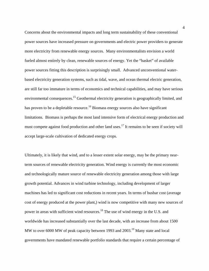
Current methods of producing electrical energy in the U.S. produce significant environmental

impacts and have limited long-term sustainability. In 2003 the U.S. derived about 70% of its

electricity from fossil sources, including coal, natural gas, and oil.1 The bulk of the remaining

electricity was produced by nuclear energy, and hydroelectric sources. Figure 1.1 illustrates the

major fuel sources for U.S. electricity generation.

Coal51%

Nuclear20%

Natural Gas17%

Other2%

Oil3%Hydro

7%

Figure 1.1: Distribution of Energy Sources for Electricity Generation in the U.S. (2003 Data)2

2The four major sources of electricity in the U.S. (coal, nuclear, natural gas, and hydro) are

considered by many to be unsustainable due either to their large-scale environmental impact, or

to limits of fuel source availability.

The U.S. has abundant coal resources, with no significant limits on supply for hundreds of years,

even at greatly increased consumption rates.3 Electricity generation from coal is considered

unsustainable due to the production of waste products that have significant impacts on land, air,

and water. Among the major byproducts of coal combustion are sulfur dioxide (SO2) and

nitrogen oxides (NOx), which are precursors to acid rain.4 Electricity generation from coal in the

U.S. in 2000 produced over 11 million tonnes of SO2, and over 4 million tonnes of NOx.5 Coal

combustion also produces a number of other pollutants with significant environmental and health

effects, such as fine particulates that contribute to regional haze and respiratory conditions, and

mercury, which is a potent toxin that bioaccumlates in animals and humans.6 Coal combustion’s

most significant byproduct, in terms of volume, is carbon dioxide (CO2), a greenhouse gas that is

considered largely responsible for anthropogenic climate change.7 The production of CO2 is

fundamental to the combustion process, and unlike mercury and oxides of sulfur and nitrogen,

CO2 cannot be easily filtered or chemically reduced through commercially demonstrated

technologies. Carbon sequestration from coal, involving capture, transport, and disposal, has yet

to be tested on any significant scale, and its economic costs and environmental impacts are

largely unknown. Large-scale restrictions on carbon emissions represent an uncertain future for

significant expansion of electricity generation from coal.

3Nuclear power is also not significantly constrained by the availability of fuel. U.S. reserves of

uranium can supply the existing reactor fleet for many hundreds of years, even with the relatively

inefficient “once-through” cycle currently used in the U.S.8 Reprocessing and breeder cycles

would provide an essentially infinite supply of nuclear fuels. Nuclear power is considered by

many to be unsustainable due to the production of radioactive waste products that remain highly

toxic for many thousands of years. Concerns about the risks associated with spent nuclear fuel,

as well as the potential for accidents and weapons proliferation have led to significant opposition

to the expansion of nuclear power. As a result of an unfavorable economic climate driven in part

by this opposition, no new nuclear plants have been ordered in the U.S. since 1979, and many

utility observers see large-scale expansion of conventional or advanced nuclear power (including

breeder cycles or fusion) unlikely in the near future.9,10

Natural gas generation is often perceived as a much cleaner source of energy than coal or nuclear

power, although it does produce significant quantities of CO2. Natural gas generation is limited

by the security and sustainability of fuel supplies in the U.S. Concerns about long-term

availability of natural gas are illustrated by recent increase in cost, with the average price of

natural gas in the U.S. roughly doubling between 1999 and 2003.11 The limitations of cost and

fuel availability will likely limit growth of natural gas based generation.12

Hydroelectric generation is not significantly expandable in the U.S. and most other parts of the

developed world.13 In addition, there is increasing pressure to remove existing large dams

because of the significant environmental impacts on river ecosystems.14 Many environmentalists

do not consider large hydroelectric facilities a “green” source of energy.

4Concerns about the environmental impacts and long term sustainability of these conventional

power sources have increased pressure on governments and electric power providers to generate

more electricity from renewable energy sources. Many environmentalists envision a world

fueled almost entirely by clean, renewable sources of energy. Yet the “basket” of available

power sources fitting this description is surprisingly small. Advanced unconventional water-

based electricity generation systems, such as tidal, wave, and ocean thermal electric generation,

are still far too immature in terms of economics and technical capabilities, and may have serious

environmental consequences.15 Geothermal electricity generation is geographically limited, and

has proven to be a depletable resource.16 Biomass energy sources also have significant

limitations. Biomass is perhaps the most land intensive form of electrical energy production and

must compete against food production and other land uses.17 It remains to be seen if society will

accept large-scale cultivation of dedicated energy crops.

Ultimately, it is likely that wind, and to a lesser extent solar energy, may be the primary near-

term sources of renewable electricity generation. Wind energy is currently the most economic

and technologically mature source of renewable electricity generation among those with large

growth potential. Advances in wind turbine technology, including development of larger

machines has led to significant cost reductions in recent years. In terms of busbar cost (average

cost of energy produced at the power plant,) wind is now competitive with many new sources of

power in areas with sufficient wind resources.18 The use of wind energy in the U.S. and

worldwide has increased substantially over the last decade, with an increase from about 1500

MW to over 6000 MW of peak capacity between 1993 and 2003.19 Many state and local

governments have mandated renewable portfolio standards that require a certain percentage of

5electricity to be generated from renewable sources.20 Much of this new capacity is expected to

be met with wind power.

Solar photovoltaic generation is significantly more expensive than many traditional sources, but

shows promise as a source of valuable peak-demand energy (particularly in the U.S.) if sufficient

cost reductions and efficiency gains occur.

Currently only a very small fraction (<1%) of the U.S. electricity supply is generated by wind

and solar energy,21 but there is significant opportunity for growth in the use of these resources.

The potential from these renewable energy sources is vast: the combined wind resources in the

upper Midwestern states is sufficient to meet the electrical energy needs of the entire U.S., if the

limitations of intermittency and transmission can be overcome with the use of enabling

technologies.22

Intermittency is a significant limitation to solar and wind based generation. Intermittency

significantly reduces the fraction of time energy is produced by a renewable resource.

A wind turbine generator rated at 1 MW peak capacity will produce anywhere between 0 and 1

MW at any particular moment in time, but on average will produce significantly less than half its

rated power. The uncontrollable and somewhat unpredictable nature of wind generation is a

significant burden on electric power systems. In addition, turbines located in many parts of the

U.S. produce more than average amounts of power during the spring, when energy is least

valuable, and less than average amounts of energy when it is most valuable: during summer

afternoons. While the fact that “the wind doesn’t always blow” and “the sun doesn’t always

6shine” may be cited as the limiting factors for the use of intermittent renewables, it is the

changes in output that often cause the most problems in some areas. Wind energy ramp rates can

be very high, going from no output to full power in as little as one hour. Solar PV generation can

produce even more rapid swings in output. Electric power systems can accept only a limited

amount of energy from sources that perform in this manner. Energy storage can address these

issues by smoothing renewable generation output and increasing reliability, predictability, and

economic value of renewable energy sources.

The other major factor limiting the use of wind energy in particular is resource location. Areas

with large amounts of wind resources are largely in the Midwestern U.S., while major load

centers are concentrated on the east and west coasts. Long distance transmission allows

Midwestern wind energy to supply energy to distant load centers. Increased transmission

capacity also increases the “spatial diversity” of wind resources, increasing the overall use of

wind energy in a large system.

The combination of intermittency and resource availability prevents renewable energy sources

like solar and wind generation from providing a significant fraction of the nation’s power supply

without the use of enabling technologies. It is important to determine if these enabling

technologies are compatible with the goals of deploying renewable energy, including increased

energy sustainability, lower greenhouse gas emissions, and reduced use of polluting fossil energy

sources. Many “life-cycle” studies of wind and solar PV systems (without storage) have

demonstrated these favorable qualities.23 If enabling technologies must be deployed for

renewable energy to provide large amounts of electrical energy, then these enabling technologies

7must also have favorable environmental characteristics to produce the desired environmental

benefits.

1.2 Objectives of this Work

To understand the potential environmental impacts of enabling technologies, the degree to which

enabling technologies are needed must first be established. This work creates a basic

intermittency cost model in an attempt to find a “break even” cost for energy storage in the

Midwestern U.S. The results of this model are used to estimate how much wind can be used

before storage becomes economically necessary for further use of this intermittent resource. The

quantitative results of this model are combined with a qualitative discussion of the system-wide

requirements of energy storage and transmission that are needed for intermittent wind energy to

provide a large fraction of the nation’s electrical energy.

To evaluate the environmental impacts associated with electricity storage and transmission,

several “life-cycle” metrics are developed. The primary measures of environmental impact used

in this work are total fossil energy usage and greenhouse gas emissions. These metrics are then

applied to a number of storage technologies considered economically and technically mature,

including compressed air energy storage (CAES), pumped hydro storage (PHS), and battery

energy storage (BES). Similar analysis is performed on transmission and distribution systems,

including both conventional AC and high voltage DC technologies.

The evaluation of energy storage and transmission system components ultimately allows for a

“systems approach” to equitably compare renewable energy sources to traditional energy

8sources. Several models of dispatchable renewable energy systems, which combine generation,

storage, and transmission, were created to compare the environmental performance of

intermittent wind and solar PV to fossil and nuclear based generation.

This work also evaluates energy storage and long distance transmission used with conventional

energy systems. While energy storage and transmission have been described as “renewable

energy enabling” technologies, they also can provide substantial economic benefits to traditional

generation sources, including coal. As with renewable energy systems, this work takes a life-

cycle approach to examine the environmental consequences of the use of energy storage with

fossil electricity generation.

This evaluation forms a framework to examine existing clean air regulations, and how the use of

energy storage effectively circumvents emission standards for new power sources. Current

emissions regulations do not sufficiently address the potential negative impacts that may result

when energy storage is combined with older coal fired power plants. This work provides a

detailed analysis of the actual emissions that result from the construction and use of a new

energy storage facility, compared to non-storage alternatives, and illustrates the energy storage

“loophole” that exists in U.S. power plant regulations. Policy options to address the use of

energy storage in an environmentally friendly manner are evaluated in terms of feasibility and

effectiveness.

This thesis makes several contributions to the interdisciplinary field of energy and environmental

analysis. Major contributions include:

9• Adding to the understanding of the limits of intermittent sources in conventional electric

power systems.

• Development of new metrics to compare energy storage systems to other electric power

technologies.

• Providing new life-cycle analysis on several different energy storage and transmission

technologies.

• Enabling a more equitable environmental comparison between intermittent and firm

sources of power.

• Addressing previously unconsidered aspects of policies regulating new energy

technologies.

1.3 Review of Literature

1.3.1 Limits of Renewable Energy without Energy Storage

Many researchers have addressed the impacts and limitations of intermittent energy sources in

electric power systems that do not incorporate energy storage. While these studies are ultimately

addressing the same issue, the impacts of intermittency, their goals and focus are quite diverse.

Some research examines the specific technical impacts on system operation. An example

includes work by Belanger and Gagnon24 who evaluate a scenario where wind provides 11% of

the total energy into a system that is largely hydro, therefore very flexible. At this penetration

rate they find considerable system disruption, resulting in alteration in river flows that could

have unacceptable environmental consequences. The study concluded that extra spinning backup

would be required, although the study did not account for import/export capacity, nor a large

geographical dispersion of wind turbines. A significant amount of research has been performed

10on technical impacts of large wind deployment in Europe. An example is work by Dany25 who

discusses the substantial increase in generation reserves necessary for wind integration in

Europe, but does not quantify the costs.

There have been a number of studies that examine the economics of wind energy use in small

power grids. Examples include Tande26 and Beyer and Degner,27 who found that wind energy

can economically provide large amounts (up to about 30%) of the energy on a small systems that

use flexible, but expensive diesel generators. However, these studies are of limited use when

examining the wind energy in large systems, particularly those in the U.S. that rely heavily on

relatively inflexible coal and nuclear generation.

Studies of the economic costs of wind intermittency in large power grids tend to take two

approaches. Some studies evaluate the decreased value of wind energy as more wind is used in

an electric power system. Examples include Grubb28 and Munter29 who both find that value of

wind falls with increased use, but arrive at significantly different conclusions. A 1988 study by

Grubb estimates that the value of wind falls by about 50% when wind contributes about 50% of

total demand over a large area in England. However, Grubb’s models provide a level of

flexibility to conventional power systems that is probably overly optimistic, and more recent

models tend to be far more conservative. Munter’s study finds that the value of wind can fall to

0 or less at wind contribution as low as 25% of total energy in South Denmark. A study in the

U.S. by Hirst and Hild30 found that the value of wind dropped by more than 2/3 when wind

produces about 25% of a system’s electrical energy.

11Most studies in the U.S. evaluate the additional costs imposed on system operation by wind

intermittency. In a 1993 report, Wan and Parsons31 review the results of early integration studies

and conclude that achieving 10% of a systems energy with renewables would not impose

significant technical or economic burdens. A significant number of studies of wind integration

costs were completed more recently. A summary of 4 such studies is provided by Parsons et al.32

These studies tend to confirm that wind providing 10% of energy imposes little addition cost, but

none of these studies examine the costs of very high wind energy penetration. These results of

these and several other studies are discussed in more detail in Chapter 2.

1.3.2 Benefits of Energy Storage to Traditional Generation

The advantages of energy storage to traditional generators have been extensively reviewed.

Examples include Boyd et al.,33 Price,34 and Linden35 who all conclude that several current

energy storage technologies including CAES and BESS can provide economic benefits to

existing generation systems

1.3.3 Methods and Metrics of Environmental Life-Cycle analysis

A variety of metrics have been developed in an attempt to compare different energy systems

from a net energy perspective. Spreng36 presents a comprehensive review of energy analysis

methods, but this review makes little attempt to utilize energy accounting as a measure of

environmental impact. The limitations of energy accounting as a measure of sustainability have

been discussed by a few authors, including Chwalowski,37 Leach38 Specific application of energy

sustainability metric to energy storage system has been applied by Rydh,39although the metrics

used by Rydh are not broadly applicable for comparisons across broad classifications of

technologies. An extensive review of the methods and metrics of environmental life-cycle

12analysis applied to electric power systems is provided by Meier.40 Meier discusses the

standard metrics used to evaluate energy sustainability including energy payback ratio, and life-

cycle energy efficiency, and demonstrates their inherent limitations as comparative metrics.

Meier also concludes that metrics currently used by the National Renewable Energy Laboratory

41, , ,42 43 44are among the most useful for comparisons across technology groups. The primary

sustainability measurement used in this work is based on the NREL metrics.

1.3.3 Environmental Analysis of Energy Storage Systems

Many technical and economic comparisons of energy storage systems have been performed.

Reviews by Kondoh et al.45 and Cavallo,46 conclude that pumped hydro storage (PHS),

compressed air energy storage (CAES), and advanced battery energy storage (BES) are the most

economic storage systems for large scale energy storage for intermittent renewables. A review of

technologies by the Electricity Storage Association47 concludes that in addition to lead-acid

batteries, flow battery technologies, including Vanadium and Polysulphide batteries are the most

economic for large scale application.

Most environmental analysis of PHS focus on biological, hydrological, or aesthetic issues.

Examples include work by Simmons and Neff,48 Clugston and U.S. Fish and Wildlife Service,49

New England River Basins Commission, 50 and U.S. Bureau of Reclamation51 that consider

ecosystem alteration, and biological impacts. Several pumped hydro projects have been proposed

since the passage of the National Environmental Policy Act (NEPA), which require an

environmental impact statement (EIS) for most major hydro projects. Examples include the

Summit Energy Storage Project52 and the River Mountain Project.53 The various studies and EIS

13documents in the literature address the significant impacts on land and water from PHS

construction and use, but do not consider net energy impacts or upstream emissions which are

the focus of this work.

While no life-cycle energy or emissions studies of PHS systems were located, a number of life-

cycle studies have been performed on conventional hydro projects, which are similar in nature to

PHS. Studies by Gagnon and Van de Vate,54 Rashad and Ismail,55 Navrud,56 Oak Ridge National

Laboratories,57 and Uchiyama58 found very low life-cycle energy requirements and greenhouse

gas emissions from hydro project construction and operation. However, ongoing studies by

Fearnside59 and Gagnon60 have found decaying biomass in flooded reservoirs can have

significant GHG consequences, although this appears to be limited to projects in tropical regions.

This is an active area of research. Most other environmental analyses on dams focus on other

environmental and social impacts, such as such as land use and displacement of native

populations, and disruption of natural habitats.

Several authors have evaluated the net efficiency of CAES including Zaugg and Stys61 and

Najjar and Zaamout62 These works do not perform a complete life-cycle assessment, nor do they

assess environmental impacts. Since CAES has many similarities to gas turbines, previous

analyses of this technology are directly applicable. Studies by Meier and Kulcinski63 and Spath

and Mann64 found significant life-cycle impacts from natural gas production and transmission

Interest in potential large scale use of electric vehicles resulted in a number of life-cycle studies

of batteries, including lead-acid batteries. Environmental assessments of lead-acid batteries

14include work by Tsoulfas et al.,65 Socolow and Thomas,66 Cobas-Flores et al.,67 Lankley and

Micheael68 and Steele and Allen.69 Wronski70 and Rade and Andersson71 reviews life-cycle

material requirements for electric vehicle batteries. Steele and Allen (1996)72 discusses recycling

impacts. Since many of these studies focus on transportation, their conclusions compare life-

cycle impacts of electric vehicles compared to conventional combustion engines. While these

conclusions are not particularly relevant to this work, the data and analysis of the batteries

themselves were used in this analysis.

There is limited assessment of flow batteries, a more recent technology likely to be used for

energy storage applications. Several economic comparisons have been published include work

by Lotspeich73 and McDowall.74 A life-cycle assessment of several flow battery technologies has

been performed by Rydh,75,76 including a life-cycle comparison between Vanadium and Lead-

acid batteries. The Tennessee Valley Authority77 prepared an environmental impact statement for

the proposed Regenesys polysulphide battery, which focuses primarily on land use and potential

toxic chemical release.

1.3.4 Environmental Analysis of Transmission and Distribution Systems

Most environmental analysis of electric transmission systems focus on aesthetics, land use,

wildlife impacts or possible health effects related to EMF. Examples include studies by DeCicco

and Beyea,78 Hammons,79 Knoepfel,80 and Hull and Bishop.81 Among the more significant

conclusions from this body of work is that high voltage DC is generally preferable to

conventional AC due to its overall lower footprint for a given power rating.

15The review of literature performed for this work, as well as other published reviews such as

Bergeson and Lave82 and Curran et al.83 have found that the effects of T&D are generally

ignored or addressed superficially by most life-cycle studies. There are a few international

studies related to the life-cycle energy studies related to T&D systems, including Dethlefsen et

al.,84 who examines the T&D system in Sweden and Uchiyama85 who examines T&D in Japan.

In both of these studies, the analysis of T&D is a relatively minor part, with little details

regarding methods or comprehensive results.

There are a number of life-cycle studies on individual T&D system components. The results of

many of these studies were incorporated into this work to develop system-wide analysis.

Examples of component studies include a comparative LCA on transformer insulators performed

by Sakai and Hoshino86 Preisegger et al.87 who found net environmental benefits of sulfur

hexaflouride compared to other insulating materials. Studies by Kunniger and Richter88 and

Erlandsson and Edlund89 found wood to be superior to other materials in terms of energy usage

and GHG emissions for utility power poles. This study also used previous life-cycle studies of

transformers performed by the Green Design Initiative.90

1.3.5 Environmental Analysis of Integrated Renewable Energy/Storage Systems

A very large number of studies have been published on the energy and environmental

performance of wind turbines. A recent review of results is provided by Lenzena and

Munksgaardb.91 However, no comprehensive environmental performance analysis of a combined

wind/CAES or wind/PHS system was found. A number of studies have been published

describing the technical and economic performance of combined wind/storage systems.

16Sorenson92 published an analysis in 1976 that found wind/storage systems could produce

“baseload” performance from wind energy. Previous evaluation of the technical performance of

a combined wind/pumped hydro has been performed by Loewus and Millham93 and Bollmeier.94

The use of CAES for wind energy storage has been suggested at least as early as 1990 by

Bogdanic and Buden.95 More recently, Cavallo analyzed the various storage and transmission

technologies and concluded that a wind/CAES/HVDC system is the most likely scenario for

large scale use of wind energy.96, ,97 98 Cavallo models such systems and find such systems can

provide high capacity factors and reasonable economic performance compared to conventional

systems. Similar analysis has been applied to systems in China by Lew et al.99 DeCarolis and

Keith100 provides an economic analysis of more modern wind/CAES/HVDC systems considering

carbon taxes on fossil sources, and discusses emission reduction benefits of a wind/CAES

system. The economic and technical performance of a specific wind/CAES system in Texas has

been analyzed by Desai et al.101 and Desai and Pemberton.102 None of the above studies performs

a comprehensive life-cycle analysis, nor to they provide details results about fuel usage over a

variety of operating scenarios.

There is a substantial body of work on the environmental performance of PV systems deployed

without storage. Examples include Meier and Kulcinski103 and Keoleian and Lewis.104 There are

also a number of environmental assessments of integrated PV/Battery systems including work by

Alsema,105 Celik,106 and Johnson et al.107 These existing studies evaluate stand-alone systems

using lead-acid or nickel cadmium batteries sized to deliver power for off-grid applications.

Recent work by Rydh108 evaluates the performance of PV systems with advanced batteries, but

the analysis is based on continuous duty, not peaking duty, which was the primary focus of this

17study. Existing studies have demonstrated PV/BESS systems to be superior to fossil-based

systems, in terms of resource sustainability and GHG emissions, but limited by the energy

intensity of the storage system compared to most other non-combustion energy systems. There

are a number of studies of the technical or economic performance of PV/battery systems for

peaking duties. These studies, include work by Marwali,109 Chowdhury and Rahman,110 Borrowy

and Salameh,111 Muselli et al.112 and Largen et al.113 were used to estimate the battery size

requirements for this work.

1.3.6 Environmental and Policy Assessment of Fossil/Storage Systems

A review of literature found that most policy and legal concerns related to future energy storage

systems involve unique aspects of individual technologies. Examples include a discussion of

potential impacts of magnetic fields from the use of superconducting magnetic energy storage by

Wolsky,114 and a discussion by Moy115 of the legal concerns related to hazards associated with

the use hydrogen gas for energy storage.

Most research appears to overlook potential negative air emissions consequences of utility scale

energy storage used with existing sources. For example, Gallob116 and Baumann117 discuss the

potential environmental benefits of using SMES energy storage, focusing mainly on increased

utilization and efficiency of existing plants, and decreasing the need for new plants. There are a

number of studies that directly or indirectly analyze the use of environmental impacts of energy

storage, including CAES, with fossil plants, including Bradshaw and Brewer118 and Lee and

Hall.119 However, these studies generally do not compare the use of storage with older, dirtier

plants, with the constructing newer, cleaner plants. These studies also do not consider the

18

compatibility of increasing output at older plants with existing clean air regulations. This area

of study is particularly suited to a more comprehensive, interdisciplinary approach, which

combines a technical analysis of existing generation, with a legal and policy analysis of the intent

and goals of existing U.S. clean air legislation.

1.4 Chapter References

1 U.S Department of Energy (2004). Electric Power Monthly March 2004. Energy Information Administration, Office of Coal, Nuclear, Electric and Alternate Fuels. Washington, DC. DOE/EIA-0226 (2004/03).

2 Ibid. 3 U.S Department of Energy (1999). U.S. Coal Reserves: 1997 Update. Energy Information

Administration, Office of Coal, Nuclear, Electric and Alternate Fuels. Washington, DC. DOE/EIA-0529(97).

4 Ramage, J. (1997). Energy: A Guidebook, Oxford University Press. 5 U.S. Environmental Protection Agency (2004). Via

http://www.epa.gov/cleanenergy/egrid/highlights.html#totals, Accessed Feb 13, 2004. 6 Wisconsin Department of Natural Resources (1999). Recommended Strategy for Mercury

Reductions to the Atmosphere in Wisconsin. 7 Ramage, J. (1997). 8 U.S Department of Energy (2001). Uranium Industry Annual 2000. Energy Information

Administration, Office of Coal, Nuclear, Electric and Alternate Fuels. Washington, DC. DOE/EIA-0478(2000).

9 Numark;, N. J. and M. O. Terry (2003). New nuclear construction: Still on hold. Public

Utilities Fortnightly 141(22): pp. 32. 10 Deutch, J., et al. (2003). The Future of Nuclear Power: An Interdisciplinary MIT Study.

Massachusetts Institute of Technology. Cambridge, MA. 11 U.S Department of Energy (2004). Via http://tonto.eia.doe.gov/dnav/ng/hist/n9190us3M.htm,

Accessed April 12, 2004.

19 12 Attanasi, E. (2001). U.S. Gas Production: Can We Trust the Projections? Public Utilities

Fortnightly 139(15): pp. 12-19. 13 Ramage, J. (1997). 14 Anon. (2000). Saving the Snake River Salmon. The New York Times. April 2, 2000. Section

4; Page 14. 15 Ramage, J. (1997). 16 Ramage, J. (1997). 17 Pimentel, D., et al. (2002). Renewable Energy: Current and Potential Issues. BioScience

52(12). 18 American Wind Energy Association (2004) The Economics of Wind Energy. Via

http://www.awea.org/pubs/factsheets/EconomicsofWind-March2002.pdf. 19 American Wind Energy Association (2004) Via http://www.awea.org/faq/instcap.html,

Accessed April 18, 2004. 20 Murphy, K. (2004). States set example with green power policies. Stateline.org March 26,

2004. At http://www.stateline.org/stateline/?pa=story&sa=showStoryInfo&id=360123. 21 U.S Department of Energy (2004). 22 Petersik, T. (1999). Modeling the Costs of U.S. Wind Supply. Issues in Midterm Analysis and

Forecasting. U.S. Department of Energy. Washington D.C. DOE/EIA-0607(99). 23 Gagnon, L., et al. (2002). Life-cycle assessment of electricity generation options: The status of

research in year 2001. Energy Policy 30(14): pp. 1267-1278. 24 Belanger, C. and L. Gagnon (2002). Adding wind energy to hydropower. Energy Policy

30(14): pp. 1279-1284. 25 Dany, G. (2001). Power reserve in interconnected systems with high wind power production.

Proceedings of the 2001 IEEE Porto Power Tech Conference. 26 Tande, J. O. (2000). Assessing high wind energy penetration. Renewable Energy 6(5-6): pp.

633-637. 27 Beyer, H. G. and T. Degner (1997). Assessing the maximum fuel savings obtainable in simple

wind-diesel systems. Solar Energy 61(1): pp. 1-64.

20 28 Grubb, M. J. (1988). The economic value of wind energy at high power system penetrations:

an analysis of models, sensitivities and assumptions. Wind Engineering 12(1). 29 Munter, P. (1999) RE-Value2 activity report for task A4. 30 Hirst, E. and J. Hild (2004). Integrating Large Amounts of Wind Energy with a Small Electric-

Power System. 31 Wan, Y.-h. and B. K. Parsons (1993). Factors Relevant to Utility Integration of Intermittent

Renewable Technologies. National Renewable Energy Laboratory. Golden, CO. NREL/TP-463-4953.

32 Parsons, B., et al. (2003). Grid Impacts of Wind Power: A Summary of Recent Studies in the

United States. Proceedings of the European Wind Energy Conference, Madrid, Spain. 33 Boyd, D. W., et al. (1983). Assessment of Market Potential of Compressed-Air Energy-Storage

Systems. Journal of Energy 7(6): pp. 549-556. 34 Price, A. (2000). The future of energy storage in a deregulated environment. IEEE 2000

Power Engineering Society Summer Meeting, Piscataway, NJ, USA. 35 Linden, S. v. d. (2002). CAES For Today’s Market. EESAT 2002 Electrical Energy Storage -

Applications and Technology, San Francisco, CA. 36 Spreng, D. (1988). Net Energy Analysis and the Energy Requirements of Energy Systems.,

Praeger Publishers, New York. 37 Chwalowski, M. (1996). Critical Questions about the Full Fuel Cycle Analysis. Energy

Conversion & Management 37(6-8): pp. 1259-1263. 38 Leach, G. (1975). Net Energy Analysis: Is it Any Use? Energy Policy 3(4). 39 Rydh, C. J. (2003). Energy Analysis of Batteries in Photovoltaic Systems. Electrical Energy

Storage - Applications and Technology, San Francisco, CA. 40 Meier, P. J. (2002). Life-Cycle Assessment of Electricity Generation Systems and

Applications for Climate Change Policy Analysis, Ph.D. Dissertation, University of Wisconsin - Madison.

41 Summary and Recommendations: Total Fuel Cycle Assessment Workshop. (1995). NREL

Report No. TP-463-7671. 42 Fuel Cycle Assessment: A Compendium of Models, Methodologies and Approaches. (1994).

NREL Report No. TP-463-6155.

21 43Spath, P. L., et al. (1999). Life Cycle Assessment of Coal-fired Power Production. National

Renewable Energy Laboratory. Golden, Colorado. NREL/TP-570-25119. 44 Spath, P. L. and M. K. Mann (2000). Life Cycle Assessment of a Natural Gas Combined-Cycle

Power Generation System. National Renewable Energy Laboratory. Golden, CO. NREL/TP-570-27715.

45 Kondoh, J., et al. (2000). Electrical energy storage systems for energy networks. Energy

Conversion and Management 41(17): pp. 1863-74. 46 Cavallo, A. J. (2001). Energy Storage Technologies for Utility Scale Intermittent Renewable

Energy Systems. Journal of Solar Energy Engineering 123: pp. 387-389. 47 Electricity Storage Association (2002) Via

http://www.electricitystorage.org/technology/ratings.htm. Accessed 8/27/02. 48 Simmons, G. M. and S. E. Neff (1969). The effect of pumped-storage reservoir operation on

biological productivity and water quality. Blacksburg, Water Resources Research Center, Virginia Polytechnic Institute.

49 Clugston, J.P. and U.S. Fish and Wildlife Service (1980). Proceedings of the Clemson

Workshop on Environmental Impacts of Pumped Storage Hydroelectric Operations, Clemson, South Carolina, U.S. Dept. of the Interior Fish and Wildlife Service Southeast Reservoir Investigations. U.S. Dept. of the Interior Fish and Wildlife Service Southeast Reservoir Investigations.

50 New England River Basins Commission (1972). An environmental profile system for

comparison of pumped storage versus gas turbine plants for peaking power production. 51 United States Bureau of Reclamation and Colorado State University (1993). Aquatic ecology

studies of Twin Lakes, Colorado 1971-86 effects of a pumped-storage hydroelectric project on a pair of montane lakes. U.S. Bureau of Reclamation. Denver, CO.

52 United States. Office of Hydropower Licensing. and Summit Energy Storage Inc., (1991).

Final environmental impact statement proposed Summit pumped storage hydroelectric project, Summit County, Ohio. Washington, D.C., Office of Hydropower Licensing.

53 United States. Office of Hydropower Licensing., (1994). Final environmental impact statement

River Mountain pumped storage hydroelectric project, Logan County, Arkansas : FERC no. 10455. Washington, DC, The Office of Hydropower Licensing.

54 Gagnon, L. and J. Van de Vate (1997). Greenhouse gas emissions from hydropower. Energy

Policy 25(1): pp. 7-13.

22 55 Rashad, S. M. and M. A. Ismail (2000). Environmental-impact assessment of hydro-power in

Egypt. Applied Energy 65(1-4): pp. 285-302. 56 Navrud, S. (2001). Environmental costs of hydro compared with other energy options.

International Journal on Hydropower & Dams 8(2): pp. 44-48. 57 Oak Ridge National Laboratory and Resources for the Future. (1992-1996). Estimating

Externalities of Fuel Cycles. Utility Data Institute and the Integrated Resource Planning Report. USA.

58 Uchiyama, Y. (1996). Life Cycle Analysis of Electricity and Supply Systems: Net energy

analysis and greenhouse gas emission. Proceedings of a Symposium on Electricity, Health and the Environment: Comparative Assessment in Support of Decision Making, IAEA-SM-38/33, Vienna.

59 Fearnside, P. M. (2002). Greenhouse Gas Emissions from a Hydroelectric Reservoir (Brazil's

Tucurui Dam) and the Energy Policy Implications. Water, Air, & Soil Pollution 133(1-4): pp. 69-96.

60 Gagnon, L. (1993). Emissions from Hydroelectric reservoiurs and comparison of

hydroelectric, natural gas, and oil. Ambio 22: pp. 568-569. 61 Zaugg, P. and Z. S. Stys (1980). Air-Storage Power Plants with Special Consideration of USA

Conditions. Brown Boveri Review 67: pp. 723-733. 62 Najjar, Y. S. H. and M. S. Zaamout (1998). Performance analysis of compressed air energy

storage (CAES) plant for dry regions. Energy Conversion & Management 39(15): pp. 1503-1533.

63 Meier, P. J. and G. L. Kulcinski (2000). Life-Cycle Energy Cost and Greenhouse Gas

Emissions for Gas Turbine Power. Energy Center of Wisconsin. Research Report 202-1. 64 Spath, P. L. and M. K. Mann (2000). 65 Tsoulfas, G. T., et al. (2002). An environmental analysis of the reverse supply chain of SLI

batteries. Resources, Conservation and Recycling 36(2): pp. 135-154. 66 Socolow, R. and V. Thomas (1997). The Industrial Ecology of Lead and Electric Vehicles.

Journal of Industrial Ecology 1(1): pp. 13-36. 67 Cobas-Flores, E., et al. (1996). Life cycle analysis of batteries using economic input-output

analysis. Proceedings of the 1996 IEEE International Symposium on Electronics and the Environment

23 68 Lankey, R. L. and F. C. Micheael (2000). Life-Cycle Methods for Comparing Primary and

Rechargeable Batteries. Environmental Science & Technology 34: pp. 2299-2304. 69 Steele, N. L. C. and D. T. Allen (1998). An abridged life-cycle assessment of electric vehicle

batteries. Environmental Science & Technology 32(1): pp. 40A-46A. 70 Wronski, Z. S. (2001). Materials for rechargeable batteries and clean hydrogen energy

sources. International Materials Reviews 46(1): pp. 1-49. 71 Rade, I. and B. A. Andersson (2001). Requirement for metals of electric vehicle batteries.

Journal of Power Sources 93(1-2): pp. 55-71. 72 Steele, N. and D. Allen (1996). Evaluation of recycling and disposal options for batteries.

Proceedings of the 1996 IEEE International Symposium on Electronics and the Environment. 73 Lotspeich, C. (2002). A Comparative Assessment of Flow Battery Technologies. Electrical

Energy Storage - Applications and Technology Conference, San Francisco, CA. 74 McDowall, J. (2001). Battery life considerations in energy storage applications and their

effect on life cycle costing. Power Engineering Society Summer Meeting, 2001. 75 Rydh, C. J. (2001). Environmental Assessment of Battery Systems in Life Cycle Management.

Department of Technology, University of Kalmar. Göteborg, Sweden, Chalmers University of Technology.

76 Rydh, C. J. (1999). Environmental assessment of vanadium redox and lead-acid batteries for

stationary energy storage. Journal of Power Sources 80: pp. 21-29. 77 Tennessee Valley Authority (2001). Environmental Assessment: The Regenesys Energy

Storage System. Tennessee Valley Authority. Muscle Shoals, Alabama. 78 DeCicco, J. M. B., S.S. and Beyea, J. (1992). Environmental Concerns Regarding Electric

Power Transmission in North America. Energy Policy 20(1): pp. 30-39. 79 Hammons, T. J. (2001). Environmental Implications and Potential of International High-

Voltage Connections. Electric Power Components and Systems 29(11): pp. 1035-1059. 80 Knoepfel, I. H. (1996). A framework for environmental impact assessment of long-distance

energy transport systems. Energy 21(7-8): pp. 693-702. 81 Hull, R. B. and I. D. Bishop (1988). Scenic Impacts of Electricity Transmission Towers - The

Influence of Landscape Type and Observer Distance. Journal Of Environmental Management 27(1): pp. 99-108.

24 82 Bergerson, J. and L. Lave (2002). A Life Cycle Analysis of Electricity Generation

Technologies: Health and Environmental Implications of Alternative Fuels and Technologies. Carnegie Mellon

Electricity Industry Center. 83 Curran, M. A., et al. (2002). Report on the International Workshop on Electricity Data for Life

Cycle Inventories Held at the Breidenbach Research Center, Cincinnati, Ohio, October 23-25, 2001. Environmental Protection Agency. EPA/600/R-02/041.

84 Dethlefsen, U., et al. (1998). Vattenfall's Electricity Production System - A Quantitative and

Qualitative Study of Emissions of Greenhouse Gases Throughout the Life-Cycle. 17th World Energy Congress held in Houston, Texas, USA in September 1998.

85 Uchiyama (1996). 86 Sakai, K. and S. Hoshino (1996). Environmental assessment of gas-insulated power-

distribution transformers. Mitsubishi Electric Advance 74: pp. 15-17. 87 Preisegger, E., et al. (2001). Life cycle assessment-electricity supply using SF6 technology.

Proceedings of 2001 International Symposium on Electrical Insulating Materials. 88 Kunniger, T. and K. Richter (1995). Life Cycle Analysis of Utility Poles, A Swiss Case Study.

Proceedings of the 3rd International Wood Preservation Symposium: The Challenge – Safety and Environment, Cannes-Mandelieu, France.

89 Erlandsson M., K. O., and M.L. Edlund (1992). Environmental consequences of various

materials to utility poles – A life cycle analysis. 23rd Annual Meeting of IRG/Stockholm. 90 Green Design Initiative (2003) Economic Input-Output Life Cycle Assessment. Sectors for

Electrical Equipment, Appliances, and Lighting. Via http://www.eiolca.net/cgi-bin/multimatrix/browse.pl Accessed July 17, 2003.

91 Lenzena, M. and J. Munksgaardb (2002). Energy and CO2 life-cycle analyses of wind

turbines—review and applications. Renewable Energy 26: pp. 339–362. 92 Sorenson, B. (1976). Dependability of Wind Energy Generators with Short-Term Energy

Storage. Science 194(4268). 93 Loewus, D. and C. B. Millham (1984). Simulating the productivity of a wind-powered

pumped-storage power facility. Energy Engineering 81: pp. 4-28.

25 94 W. Bollmeier, et al. (1994). Wind/pumped-hydro integration and test project: preliminary

system test results. Symposium Proceedings for Wind Energy 1994 The Energy-Source Technology Conference, New Orleans, Louisiana.

95 Bogdanic, A. and R. Budin (1990). Compressed air as wind energy storage. Energy and the

Environment Into the 1990s. Proceedings of the 1st World Renewable Energy Congress. Pergamon, Oxford,

UK. 96 Cavallo, A. J. (1995). High-Capacity Factor Wind Energy Systems. Journal of Solar Energy

Engineering 117: pp. 137-143. 97 Cavallo, A. (1996). Transforming Intermittent Wind Energy To A Baseload Power Supply

Economically. Power-gen '96 : the Ninth International Power Generation Exhibition & Conference, Orlando, Florida.

98 Cavallo, A. J. (1997). Utility scale baseload wind energy plants. Proceedings of the American

Power Conferences, Chicago, IL, (USA). 99 Lew, D. J., et al. (1998). Large scale baseload wind power in China. Natural Resources Forum

22(3): pp. 165-184. 100 DeCarolis, J. and D. W. Keith. (2002). Is the Answer to Climate Change Blowing in the

Wind? Proceedings of the first International Doctoral Consortium on Technology, Policy, and Management., Delft, The Netherlands, Delft University.

101 Desai, N., et al. (2003). Study of Electric Transmission in Conjunction with Energy Storage

Technology. Texas State Energy Conservation Office. 102 Desai, N. and D. Pemberton (2003). Economic Value of Compressed Air Energy Storage in

Conjunction with Large Scale Wind in McCamey. Ridge Energy Storage & Grid Services, LP. 103 Meier, P. J. and G. L. Kulcinski (2002). Life-Cycle Energy Requirements and Greenhouse

Gas Emissions for Building-Integrated Photovoltaics. Energy Center of Wisconsin Research Report 210-1.

104 Keoleian, G. A. and G. M. Lewis (2003). Modeling the life cycle energy and environmental

performance of amorphous silicon BIPV roofing in the US. Renewable Energy 28: pp. 271–293.

105 Alsema, E. A. (1998). Energy Requirements and CO2 Mitigation Potential of PV systems.

BNL/NREL Workshop "PV and the Environment 1998", Keystone, CO.

26 106 Celik, A. N. (2003). Techno-economic analysis of autonomous PV-wind hybrid energy

systems using different sizing methods. Energy Conversion and Management 44(12): pp. 1951-1968.

107 Johnson, A. J., et al. (1997). A Life Cycle Assessment of Grid, Grid Connected PV and Stand-

alone PV Power Systems for Household Energy Supply. 14th European PVSEC, Barcelona, Spain.

108 Rydh, C. J. (2003). Energy Analysis of Batteries in Photovoltaic Systems. Electrical Energy

Storage - Applications and Technology, San Francisco, CA 109 Marwali (1998). Short term generation scheduling in photovoltaic-utility grid with battery

storage. IEEE Transactions on Power Systems. 13(3): pp. 1057-1062. 110 Chowdhury, B. H. and S. Rahman (1988). Analysis of interrelationships between photovoltaic

power and battery storage for electric utility load management. IEEE Transactions on Power Systems 3(3): pp. 900-907.

111 Borowy, B. S. and Z. M. Salameh (1996). Methodology for optimally sizing the combination

of a battery bank and PV array in a wind/PV hybrid system. IEEE Transactions on Energy Coversion 11(2): pp. 367-375.

112 Muselli, M., et al. (2000). PV-hybrid power systems sizing incorporating battery storage: an

analysis via simulation calculations. Renewable Energy 20(1): pp. 1-7. 113 Largen, R., et al. (1993). Improved PV System Performance Using Vanadium Batteries.

Proceedings IEEE 23rd Photovoltaic Specialists Conference, Louisville, Kentucky. 114 Wolsky, A. (2000). Environment, safety, and health impact of HTS power equipment. IEEE

Power Engineering Review 20(6): pp. 12-15. 115 Moy, R. (2003). Tort Law Considerations for the Hydrogen Economy. Energy Law Journal

24(2): pp. 349-363. 116 Gallob, J. A. (1990). In Search of Beneficial Environmental Impacts: Superconductive

Magnetic Energy Storage, The National Environmental Policy Act and an Analysis of Environmental Benefits. Harvard Environmental Law Review 14: pp. 411-486.

117 Baumann, P. D. (1992). Energy conservation and environmental benefits that may be realized

from superconducting magnetic energy storage. IEEE Transactions on Energy Conversion 7(2): pp. 253 -259.

27 118 Bradshaw, D. T. and J. E. Brewer (1992). Potential strategic operating and environmental

benefits of TVA's compressed air energy storage (CAES) program. Proceedings of the American Power Conference.54 pt 1.

119 Lee, S. T. and J. A. Hall (1993). Utility application study of energy storage dynamic benefits

using dynastore. Proceedings of the American Power Conference, Chicago, IL.55 pt. 2.

28

2. The Need for Renewable Energy Enabling Technologies

Two general categories of renewable energy enabling technologies are analyzed in this work:

energy storage and long distance transmission. A study of these technologies is motivated by the

limitations of generating electric power with intermittent solar and wind resources.

This chapter presents a basic analysis of the limitations of intermittent energy sources without

the use of energy storage and increased transmission. It also provides a discussion of how

renewable enabling technologies can provide economic benefits to traditional generation sources.

The result of this analysis demonstrates the high level of motivation that exists for the

development and use of energy storage and long distance transmission in the U.S.

2.1 The Limitations of Wind Energy without Energy Storage

It is often quoted that wind energy can provide up to 10-20% of a system’s demand. Beyond this

point, it is hypothesized, wind energy becomes too expensive due to the problems imposed by

wind intermittency. The question of how much wind energy can be integrated into an electric

power system is economic as much as technical. As the use of wind energy increases its value

drops, or its cost rises, depending on one’s perspective. The origin of the 10-20% value is

unclear, but it appears to hold up reasonably well as a rough estimate of the potential role of

wind energy.

The purpose of this section is to provide an overview of the technical issues associated with the

use of wind energy, and provide a basic economic analysis of the cost of wind energy

29

integration. Wind energy systems must be effectively integrated into the existing power

system, which is fundamentally based on providing instantaneous response to electric demand.

Wind energy can be described as a source of negative demand, which is highly variable, largely

uncontrollable, and somewhat unpredictable. The use of wind energy introduces additional

variation in normal electricity demand patterns. When a relatively small amount of wind is added

to an electric power system, this variation can be accommodated by utilities, just as normal

changes in demand are accommodated. As the use of wind energy increases, its output variations

add additional technical and economic burdens on the system. Energy storage is an effective

method of dealing with intermittency, and allows greater use of wind energy than would

otherwise be possible. To determine the limits of wind energy without storage, and the potential

benefits of energy storage, the economic effects of wind energy on electric power systems must

be evaluated.

2.1.1 Operation of Conventional Electric Power Systems

Electric power systems must respond to the instantaneous consumer demand, which constantly

varies as a function of time of day and season, depending on the requirements for heat, light, and

other services provided by electricity. Instantaneous electricity demand is dominated by the daily

demand cycle, illustrated by Figure 2.1, a set of four weekly demand curves in the year 2001 for

the service territory of Madison Gas and Electric (MGE), a regulated utility located in Madison,

Wisconsin. The plots are smoothed curves based on average demand in one-hour increments.

Each of the four plots begins on a Monday, and there is a noticeable drop in demand during the

weekends. Figure 2.1 also demonstrates the seasonal variation in demand, driven by heating,

cooling, and lighting. The peak demand is driven by air conditioning requirements in late

30

afternoons on hot summer days. Minimum demand generally occurs in the spring, when

heating and cooling loads are at a minimum.

200

300

400

500

600

700

800

0 24 48 72 96 120 144 168

Hour

Dem

and

(MW

)

Summer PeakTypical SummerTypical WinterSpring Minimum

Figure 2.1: Weekly Load Patterns for Madison Gas and Electric (2001 data)1

There are a number of important features on this graph that heavily influence the manner in

which utilities construct and operate electric generation facilities, including wind. The most

obvious is the presence of large, rapid swings in power output on a daily basis, typically equal to

30% to 40% of the peak load. However, these swings are also very predictable. Utilities can

accurately predict demand on a day-ahead and hour-ahead basis, using historical records,

weather forecasts and a variety of modeling techniques that have been updated and refined over

the many decades of regulated electric utility service.2 This predictability is used to dispatch

various power plants in a “merit order” based on the marginal cost of producing electricity.

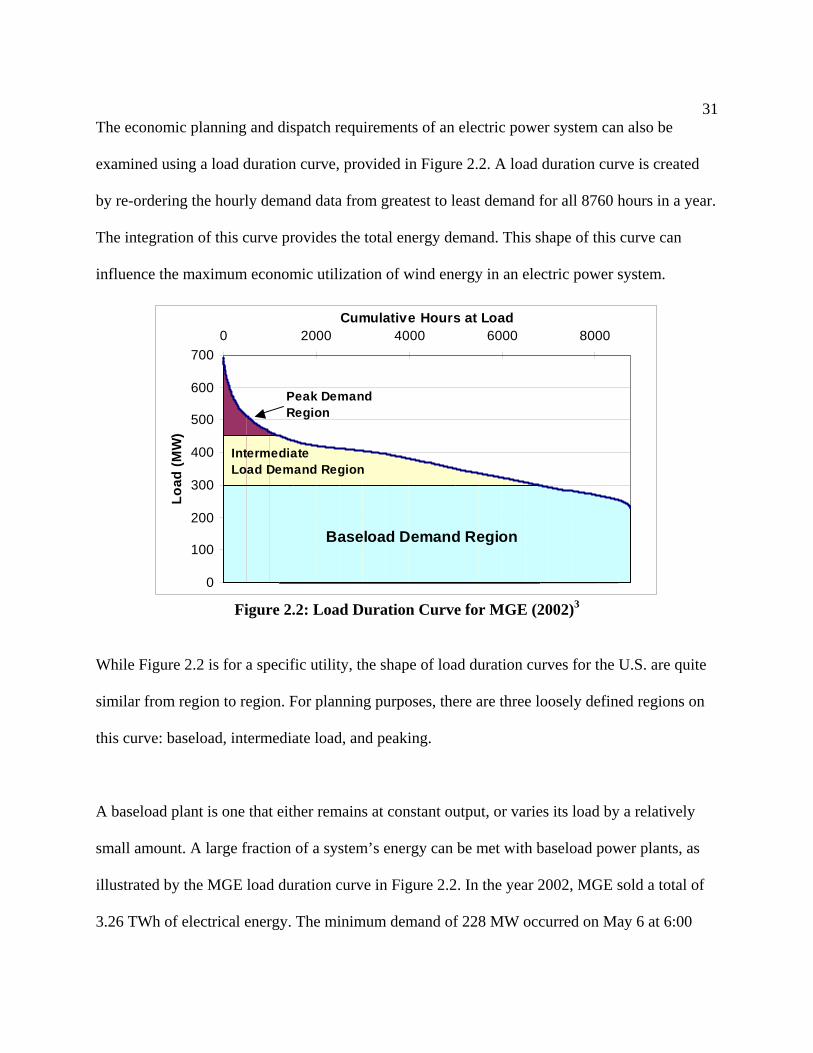
31

The economic planning and dispatch requirements of an electric power system can also be

examined using a load duration curve, provided in Figure 2.2. A load duration curve is created

by re-ordering the hourly demand data from greatest to least demand for all 8760 hours in a year.

The integration of this curve provides the total energy demand. This shape of this curve can

influence the maximum economic utilization of wind energy in an electric power system.

0

100

200

300

400

500

600

700

Load

(MW

)

0 2000 4000 6000 8000Cumulative Hours at Load

Baseload Demand Region

Intermediate Load Demand Region

Peak Demand Region

Figure 2.2: Load Duration Curve for MGE (2002)3

While Figure 2.2 is for a specific utility, the shape of load duration curves for the U.S. are quite

similar from region to region. For planning purposes, there are three loosely defined regions on

this curve: baseload, intermediate load, and peaking.

A baseload plant is one that either remains at constant output, or varies its load by a relatively

small amount. A large fraction of a system’s energy can be met with baseload power plants, as

illustrated by the MGE load duration curve in Figure 2.2. In the year 2002, MGE sold a total of

3.26 TWh of electrical energy. The minimum demand of 228 MW occurred on May 6 at 6:00

32

am. A power plant that produced a constant 228 MW over the year would produce a total of

2.00 TWh, or 61% of MGE’s total demand. This means that despite the tremendous variations in

load, a plant that does not or cannot vary load could meet well over half of MGE’s electricity

supply. An analysis of 7 utility systems in the U.S., including large utility areas in California,

Texas, New England, Pennsylvania, Wisconsin, and Minnesota found that about 60% of total

demand could be met with plants that do not cycle.4 An even greater fraction of the total demand

is met by plants whose output is almost always constant. For MGE, 65% of the load is met by

plants whose output can remain constant for 99% of the time.

Baseload plants are used to “fill” most of the bottom half of the load duration curve because they

have characteristics that are suited for continuous operation with low operation costs.

Intermediate load plants are typically used to fill the daily demand “bump” in the mid-day,

illustrated in Figure 2.1. Peaking plants primarily provide energy during the summer peak, and

may operate for only a few hundred hours per year.

Using these basic characteristics of electricity supply and demand, including the hourly load data

used to create Figure 2.2, an evaluation of the economic limitations of wind energy without

storage can be performed. Sections 2.1.2-2.1.5 describe several progressively more advanced

economic models that examine the economic advantages of using energy storage with wind

energy generation.

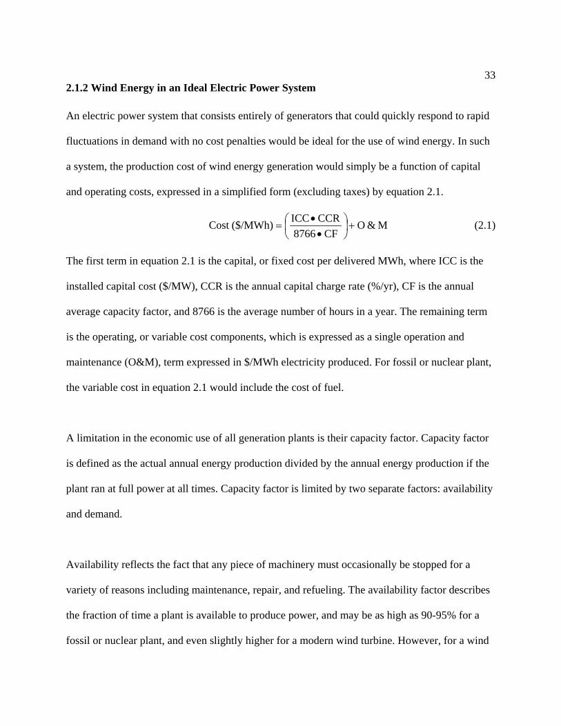
33

2.1.2 Wind Energy in an Ideal Electric Power System

An electric power system that consists entirely of generators that could quickly respond to rapid

fluctuations in demand with no cost penalties would be ideal for the use of wind energy. In such

a system, the production cost of wind energy generation would simply be a function of capital

and operating costs, expressed in a simplified form (excluding taxes) by equation 2.1.

M&O CF 8766

CCR ICC($/MWh)Cost +⎟⎠⎞

⎜⎝⎛

••

= (2.1)

The first term in equation 2.1 is the capital, or fixed cost per delivered MWh, where ICC is the

installed capital cost ($/MW), CCR is the annual capital charge rate (%/yr), CF is the annual

average capacity factor, and 8766 is the average number of hours in a year. The remaining term

is the operating, or variable cost components, which is expressed as a single operation and

maintenance (O&M), term expressed in $/MWh electricity produced. For fossil or nuclear plant,

the variable cost in equation 2.1 would include the cost of fuel.

A limitation in the economic use of all generation plants is their capacity factor. Capacity factor

is defined as the actual annual energy production divided by the annual energy production if the

plant ran at full power at all times. Capacity factor is limited by two separate factors: availability

and demand.

Availability reflects the fact that any piece of machinery must occasionally be stopped for a

variety of reasons including maintenance, repair, and refueling. The availability factor describes

the fraction of time a plant is available to produce power, and may be as high as 90-95% for a

fossil or nuclear plant, and even slightly higher for a modern wind turbine. However, for a wind

34

turbine there is the additional aspect of fuel (wind) availability. As a result, the average

capacity factor of a wind turbine is much lower, depending on wind resources. Capacity factors

for wind turbines range from close to 0% in places with very poor wind resources, to 45% in

areas with excellent wind resources. Wind turbines considered economic generally are sited in

areas that produce capacity factors from 25-40%.

The net capacity factor of a plant may be reduced by insufficient demand. Figure 2.2 illustrates

the fact that at any given time, a large fraction of a generator fleet is sitting idle. As a capacity

factor of any generator drops, the resulting cost of electricity increases, because the fixed capital

costs are divided over a smaller amount of electricity actually sold. This limitation applies to any

type of generator, including wind turbines.

Returning to the example of an “ideal” electric power system, with its ability to vary output

without limitations, MGE could hypothetically construct 228 MW of wind energy generation,

which at an average capacity factor of 33% would provide about 20% of the total energy

supplied in this system. The cost of electricity from this system would be about 4.6 cents/kWh,

using representative values of $1000/kW for total installed capital cost, a 12% annual capital

charge rate, an average annual capacity factor (CF) of 33%, and O&M cost of $5/MWh.5 If more

than 228 MW of wind energy generation is constructed, there is a probability that wind energy

would be produced when there is no demand (assuming no increase in minimum demand.) This

excess energy must either be exported or curtailed (wind turbines must be shut down

temporarily.) If it is assumed that the utility cannot sell this excess wind energy (which is not

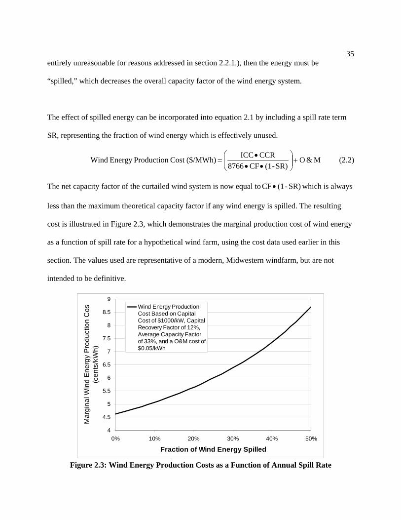
35

entirely unreasonable for reasons addressed in section 2.2.1.), then the energy must be

“spilled,” which decreases the overall capacity factor of the wind energy system.

The effect of spilled energy can be incorporated into equation 2.1 by including a spill rate term

SR, representing the fraction of wind energy which is effectively unused.

M&O SR)-(1 CF 8766

CCR ICC($/MWh)Cost ProductionEnergy Wind +⎟⎟⎠

⎞⎜⎜⎝

⎛••

•= (2.2)

The net capacity factor of the curtailed wind system is now equal to SR)-(1 CF • which is always

less than the maximum theoretical capacity factor if any wind energy is spilled. The resulting

cost is illustrated in Figure 2.3, which demonstrates the marginal production cost of wind energy

as a function of spill rate for a hypothetical wind farm, using the cost data used earlier in this

section. The values used are representative of a modern, Midwestern windfarm, but are not

intended to be definitive.

4

4.5

5

5.5

6

6.5

7

7.5

8

8.5

9

0% 10% 20% 30% 40% 50%

Fraction of Wind Energy Spilled

Mar

gina

l Win

d E

nerg

y P

rodu

ctio

n C

os(c

ents

/kW

h)

Wind Energy ProductionCost Based on CapitalCost of $1000/kW, CapitalRecovery Factor of 12%,Average Capacity Factorof 33%, and a O&M cost of$0.05/kWh

Figure 2.3: Wind Energy Production Costs as a Function of Annual Spill Rate

36

As wind energy capacity is constructed beyond the point of the minimum demand of an electric

power system, the spill rate and average production cost increase, due to the effective decrease in

capacity factor.

The spill rate that would occur in an ideal system can be estimated by comparing wind

generation data to load data. An Excel spreadsheet model was developed which superimposed

actual hourly wind energy production from a wind farm located in the Midwest6 on the MGE

hourly demand data for 2002. In this model, the size of the wind farm was scaled to provide

differing levels of supply. At each hour in time, the model compares demand to wind production,

and any energy that cannot be used is recorded as “spilled” energy. The model calculates the

spill rate by summing the total amount of energy spilled, and dividing this value by the total

wind energy produced. The average capacity factor of the wind farm for this model was 34%,

which can be compared to wind turbines in western Wisconsin that produce energy with a CF of

about 25%7, or turbines in western Minnesota that produce a annual CF of about 35%.8 An entire

year’s worth of data was used to account for seasonal variations in demand and wind energy

production.

Figure 2.4 shows the results of one possible scenario over a two-week period. In this case, wind

energy capacity of 418 MW is annually providing about 35% of the system’s total energy. The

area under the lighter shaded curve represents the total energy demand, while the solid dark line

is wind energy production. On four occasions in this two-week period, the wind energy supply

exceeds demand by as much as 150MW, and will need to be curtailed (spilled.) The dark shaded

37

area is this spilled energy, which is wind energy that the utility cannot sell, and as a result,

raises the average cost of the wind energy it can sell.

050

100150200250300350400450500

0 24 48 72 96 120 144 168 192 216 240 264 288 312 336Hour

Pow

er (M

W)

Spilled Wind Demand Wind Production

Figure 2.4: Wind Energy Production Superimposed on a MGE Hourly Load Data for a

Two-Week Period As the wind energy capacity is increased, a greater fraction of the system’s energy will be

provided by wind, but more wind energy will be spilled, increasing the average cost. Using the

annual spill rates determined by the model illustrated in Figure 2.4, the cost of wind energy can

be calculated using equation 2.2. Figure 2.5 illustrates the results of combing the spill rate data

with the cost curve in Figure 2.3

38

0%

5%

10%

15%

20%

25%

30%

35%

40%

45%

50%

20% 30% 40% 50% 60% 70%Fraction of System Energy from Wind

Perc

enta

ge o

f Win

d E

nerg

y S

pille

d

4.0

4.5

5.0

5.5

6.0

6.5

7.0

7.5

8.0

8.5

9.0

Mar

gina

l Win

d E

nerg

y P

rodu

ctio

n C

ost (

cent

s/kW

h)

Wind Energy SpilledWind Energy Cost

Figure 2.5: Spill Rate and Production Cost as a Function of Wind Energy Contribution for

the Ideal System

The wind energy cost curve in Figure 2.5 is the marginal cost, or cost of the next additional

amount of wind energy introduced into the system. In this figure, the cost of wind is constant, at

about 4.5 cents/kWh to the point where wind provides 25% of the total demand. Beyond this

contribution, additional wind energy has higher costs. At some point, the cost of wind energy

will exceed an acceptable price to a utility or consumer, and alternative generation will be

deployed. One alternative generation source would be the combination of wind energy and

storage. With storage, less of the wind generation will be spilled, which will reduce the cost of

wind energy at higher contribution. However, storage adds both capital costs and losses due to

storage inefficiencies. As a result, the cost of wind with storage will be higher than wind without

storage, at least at low penetration of wind energy. These issues are discussed in more detail in

Chapter 6. One estimate for the effective “adder” resulting from the use of storage is about 1.5 –

2.0 cents/kWh.9 The combination of wind and storage provides an alternative to wind without

39

storage, or alternative sources. In Figure 2.5, the cost of wind at low contribution is 4.5

cents/kWh, and if the storage “adder” is 2.0 cents/kWh, then the combined wind storage cost

would be about 6.5 cents/kWh. This value represents the “breakeven point” at which wind with

storage becomes more economic than simply increasing the use of wind without storage. If the

goal is to economically maximize the use of wind energy, then storage becomes necessary when

the incremental cost of wind without storage is greater than the cost of wind energy with storage,

or when the “spill cost penalty” exceeds the “storage cost penalty.” In Figure 2.5, wind energy

can deliver more than 50% of the system’s energy before storage becomes the most cost

effective method of further increasing the share of wind energy.

While this model provides a start in understanding the limitations of wind energy use, there are

several other factors to consider. Among the more important of these is the existence of “must

run” baseload generators in conventional electric power systems, which is addressed in section

2.1.3.

2.1.3 Wind Energy in an Electric Power System with Baseload Capacity

Returning to the load duration curve in Figure 2.2, it is important to recognize that an electric

utility attempts to meet electricity demand at all times at the least cost. It does so by constructing

and operating power plants with characteristics that best match the variation in demand. As

discussed in section 2.1.1, utilities can rely on a very large fraction of their energy to be

delivered by power plants that do not need to substantially vary load, and they plan and build

around this fact.

40

In the Midwest, baseload demand is met almost exclusively with nuclear and coal-fired units.

Nuclear units are held at constant output because their operational cost is very low relative to the

cost of cycling the units. Nuclear plants are also limited in their generation ramp rate, so utilities

do not risk turning down nuclear units if there is a high probability that demand may suddenly

increase. A nuclear power plant cannot simply spill excess energy, and to indicate the relative

cost of cycling, it can be noted that plant operators have actually sold electricity at negative

prices during periods of very low demand rather than reduce the power output of the plant.10 As a

result, it is extremely unlikely that a nuclear unit of any type currently used or licensed for use in

the U.S. would ever be used to respond to variations in wind energy production.

Baseload coal units are more flexible, and generally have the ability to cycle to respond to

energy demand. However, in all cases, operators of baseload coal plants avoid reducing their

output to below minimum operational levels, typically around 50% of full output.11 These units

have low operational cost while running, but high costs associated with startup and shutdown, so

utilities charge very low rates for power during periods of low demand to avoid the substantial

economic penalties associated with shutting these units down.12

The existence and use of baseload power plants reduces the amount of wind energy that can be

economically integrated into electric power systems. These baseload plants eliminate much of

the bottom half of the load duration curve from use by wind energy. Much of the area under the

curve in Figure 2.2 is effectively “filled” by must-run units, whose output cannot fall below a

certain amount without incurring substantial operational and economic penalties. The fraction of

the baseload demand met by must-run units depends on the utility and generation mix. For MGE,

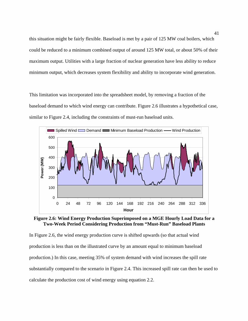
41

this situation might be fairly flexible. Baseload is met by a pair of 125 MW coal boilers, which

could be reduced to a minimum combined output of around 125 MW total, or about 50% of their

maximum output. Utilities with a large fraction of nuclear generation have less ability to reduce

minimum output, which decreases system flexibility and ability to incorporate wind generation.

This limitation was incorporated into the spreadsheet model, by removing a fraction of the

baseload demand to which wind energy can contribute. Figure 2.6 illustrates a hypothetical case,

similar to Figure 2.4, including the constraints of must-run baseload units.

0

100

200

300

400

500

600

0 24 48 72 96 120 144 168 192 216 240 264 288 312 336

Hour

Pow

er (M

W)

Spilled Wind Demand Minimum Baseload Production Wind Production

Figure 2.6: Wind Energy Production Superimposed on a MGE Hourly Load Data for a

Two-Week Period Considering Production from “Must-Run” Baseload Plants In Figure 2.6, the wind energy production curve is shifted upwards (so that actual wind

production is less than on the illustrated curve by an amount equal to minimum baseload

production.) In this case, meeting 35% of system demand with wind increases the spill rate

substantially compared to the scenario in Figure 2.4. This increased spill rate can then be used to

calculate the production cost of wind energy using equation 2.2.

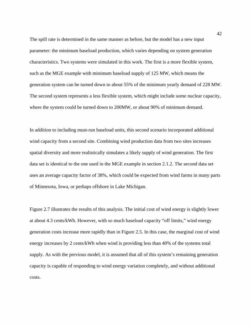
42

The spill rate is determined in the same manner as before, but the model has a new input

parameter: the minimum baseload production, which varies depending on system generation

characteristics. Two systems were simulated in this work. The first is a more flexible system,

such as the MGE example with minimum baseload supply of 125 MW, which means the

generation system can be turned down to about 55% of the minimum yearly demand of 228 MW.

The second system represents a less flexible system, which might include some nuclear capacity,

where the system could be turned down to 200MW, or about 90% of minimum demand.

In addition to including must-run baseload units, this second scenario incorporated additional

wind capacity from a second site. Combining wind production data from two sites increases

spatial diversity and more realistically simulates a likely supply of wind generation. The first

data set is identical to the one used in the MGE example in section 2.1.2. The second data set

uses an average capacity factor of 38%, which could be expected from wind farms in many parts

of Minnesota, Iowa, or perhaps offshore in Lake Michigan.

Figure 2.7 illustrates the results of this analysis. The initial cost of wind energy is slightly lower

at about 4.3 cents/kWh. However, with so much baseload capacity “off limits,” wind energy

generation costs increase more rapidly than in Figure 2.5. In this case, the marginal cost of wind

energy increases by 2 cents/kWh when wind is providing less than 40% of the systems total

supply. As with the previous model, it is assumed that all of this system’s remaining generation

capacity is capable of responding to wind energy variation completely, and without additional

costs.

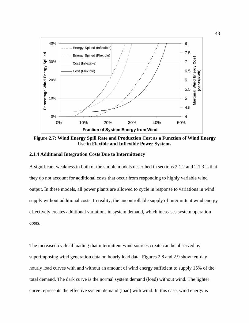
43

0%

10%

20%

30%

40%

0% 10% 20% 30% 40% 50%Fraction of System Energy from Wind

Perc

enta

ge W

ind

Ener

gy S

pille

d

4

4.5

5

5.5

6

6.5

7

7.5

8

Mar

gina

l Win

d En

ergy

Cos

t (c

ents

/kW

h)

Energy Spilled (Inflexible)

Energy Spilled (Flexible)

Cost (Inflexible)

Cost (Flexible)

Figure 2.7: Wind Energy Spill Rate and Production Cost as a Function of Wind Energy

Use in Flexible and Inflexible Power Systems

2.1.4 Additional Integration Costs Due to Intermittency

A significant weakness in both of the simple models described in sections 2.1.2 and 2.1.3 is that

they do not account for additional costs that occur from responding to highly variable wind

output. In these models, all power plants are allowed to cycle in response to variations in wind

supply without additional costs. In reality, the uncontrollable supply of intermittent wind energy

effectively creates additional variations in system demand, which increases system operation

costs.

The increased cyclical loading that intermittent wind sources create can be observed by

superimposing wind generation data on hourly load data. Figures 2.8 and 2.9 show ten-day

hourly load curves with and without an amount of wind energy sufficient to supply 15% of the

total demand. The dark curve is the normal system demand (load) without wind. The lighter

curve represents the effective system demand (load) with wind. In this case, wind energy is

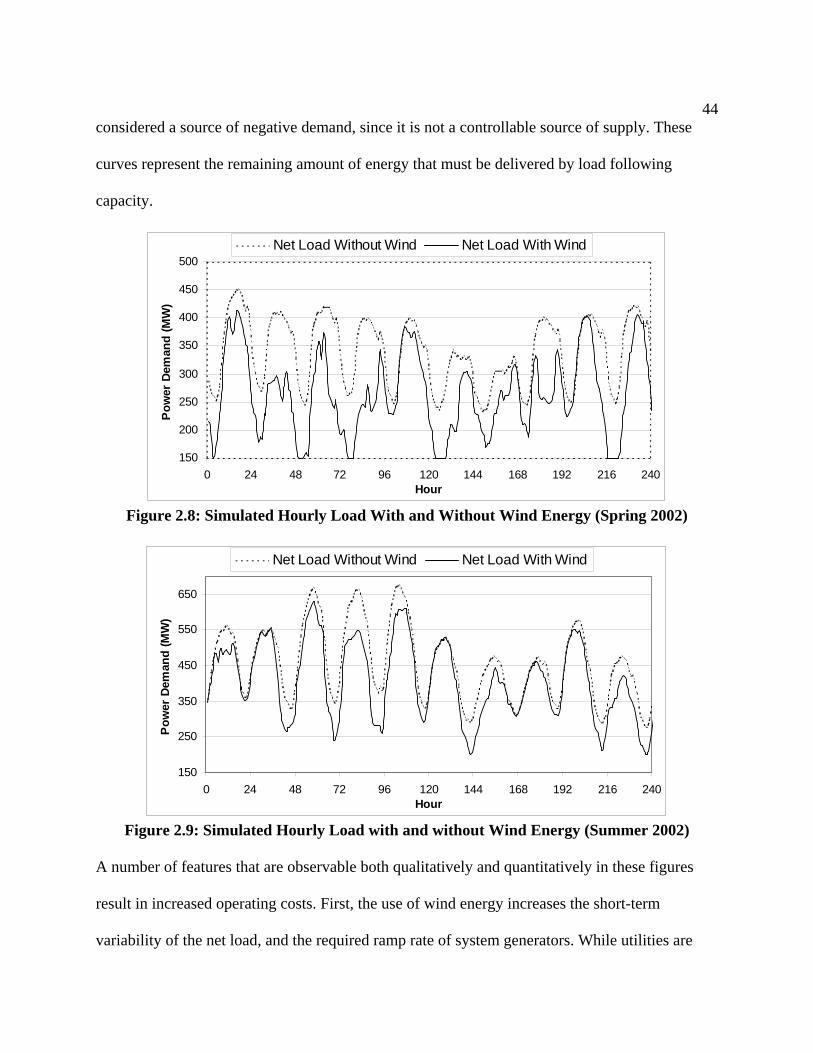
44

considered a source of negative demand, since it is not a controllable source of supply. These

curves represent the remaining amount of energy that must be delivered by load following

capacity.

150

200

250

300

350

400

450

500

0 24 48 72 96 120 144 168 192 216 240Hour

Pow

er D

eman

d (M

W)

Net Load Without Wind Net Load With Wind

Figure 2.8: Simulated Hourly Load With and Without Wind Energy (Spring 2002)

150

250

350

450

550

650

0 24 48 72 96 120 144 168 192 216 240Hour

Pow

er D

eman

d (M

W)


Figure 2.9: Simulated Hourly Load with and without Wind Energy (Summer 2002)

A number of features that are observable both qualitatively and quantitatively in these figures

result in increased operating costs. First, the use of wind energy increases the short-term

variability of the net load, and the required ramp rate of system generators. While utilities are

45

almost always adjusting their power output, ramping does result in added costs, and utilities

would like to minimize variations in load as much as possible. In the case illustrated by Figures

2.8 and 2.9, the average ramp rate increases about 12% from 7.4 MW/hour without wind to 8.3

MW/hour with wind. In addition, fluctuations in wind energy increase the number of times the

system passes through 0 in terms of generator ramping (generally from increasing load to

decreasing load or vice versa). The number of “zero crossings” increases roughly 17% from

5/day without wind to 5.7/day with wind. Finally, the fluctuations in wind energy produce a

greater number of startup and shutdowns of intermediate load and peaking power plants. Each

additional startup cycle incurs additional fuel costs, and increased O&M costs.

The use of wind energy at the level illustrated in this case also decreases the overall

predictability of the total system load, which may result in increased operational costs. The

variation of daily system demand without wind is typically quite predictable, and utilities

generally know well in advance when individual generators will be needed. Utilities schedule

generators and certain power purchase contracts on a day-ahead and hour-ahead basis. The use of

wind energy may reduce the short-term and long-term predictability of the system to the point

where generators may not be online when needed, or (more likely) generators are kept on when

not needed. Utilities also may be unable to effectively schedule wholesale power transactions.

The potential impact of predictability is striking in Figure 2.10. In this figure, wind generation

substantially reduces demand on day 3 (hours 48-72), and greatly reduces the need for firm, load

following capacity. On the very next day, however, limited wind output results in the need for

nearly all of the conventional (non-wind) generation capacity.

46

150

200

250

300

350

400

450

500

0 24 48 72 96 120 144 168 192 216 240Hour

Pow

er D

eman

d (M

W)


Figure 2.10: Simulated Hourly Load With and Without Wind Energy (Winter 2002)

A number of techniques have been developed to predict the availability of wind generation,

which reduces the penalty associated with unpredictability. However, no forecast is 100%

accurate, and studies have found wind forecasting errors can incur increased costs for utilities

that use a substantial amount of wind in their generation portfolio.13

If the costs associated with increased ramping, plant start-up, and predictability can be

quantified, they can be added to the “curtailment costs” evaluated in section 2.1.4. The

combination of these costs can improve the wind cost curves generated in Figure 2.7. This would

provide a more accurate assessment of the economic conditions necessary for the use of storage

with wind energy. However, quantifying the various costs associated with plant ramping and

startup requires extensive knowledge of the individual generator characteristics, as well as

sophisticated modeling tools. Only recently have utilities and researchers attempted to account

for the costs associated with integrating intermittent wind energy.

47

2.1.5 Utility Studies of Intermittency Costs

Utilities have begun the process of quantifying the operational costs that are incurred when wind

energy is added to an electric power system. A review of literature found seven U.S. studies that

estimate the incremental cost penalties associated wind energy integration.14-20 Each study

evaluates one or more of the three general categories of operational impacts of wind energy:

short term, long term, and reserve requirements. Short term and long term variations are

described in section 2.1.4, and include the increased cost of responding to wind energy variation

(increased ramping, uncertain unit commitment, limited certainty of market conditions etc.)

Reserve requirements consider the additional cost of spinning reserves and standby reserves that

are required for sources that cannot be reliably “controlled” such as wind.

Table 2.1 summarizes the results of these studies, providing the fraction of energy provided by

wind and the intermittency cost penalty, or “adder” which must be added to the production cost

calculated by equation 2.2 to derive the total cost of wind energy. There are several major

limitations in applying these results when calculating the intermittency penalty associated with

wind energy without storage. First, each study uses different methods and evaluates different

operational impacts of wind energy. Second, many of these studies quote wind energy

penetration in terms of power capacity, which is the ratio of installed wind capacity to peak

power demand. This makes it difficult to determine the actual fraction of the load supplied by

wind, which is a more useful measure of the ability of wind energy to provide meaningful

contribution to an electric power system. For the cases where the actual energy fraction are not

reported, it is assumed that the energy fraction is equal to ½ of the power fraction, which is a

reasonable approximation for typical utility load profiles and wind energy capacity factors.

48

Third, these studies do not address certain additional costs that may occur as a result of wind

energy use, such as increased O&M costs from increased plant cycling and efficiency reduction

due to non-optimal generator loads. Finally, the fraction of energy provided by wind in these

studies is relatively low, with the largest use of wind energy at 12% of total supply.

Table 2.1: Results of Utility Wind Integration Cost Studies Study Location % Peak

Capacity % Total Energy

Cost Adder (cents/kWh)

PJM14 East Coast 0.12 0.06* 0.03 Xcel15 Minnesota 3.5 1.75* 0.2 Pacificorp16 Northwest 20 10* 0.55 BPA17 Pacific Northwest 5.9 2.95* 0.18 WE Energies18 Eastern Wisconsin 29,15,7 12,6,3 0.29, 0.28, 0.25 CA19 California 4 2 0.17 GRE20 Minnesota 4.3,16.6 2.4,9.5 0.32, 0.45

*Indicates that % total energy is assumed to be ½ of % peak capacity The maximum integration cost in Table 2.1 is only about 0.55 cents/kWh, with wind providing

about 10% of system energy. The WE Energies study shows a smaller impact, with an

integration cost of about 0.29 cents/kWh at 12% of energy supplied by wind. These studies

indicate that a 10% energy supply from wind should have a relatively small effect on system

costs. For a wind turbine producing electricity at 4.5 cents/kWh, the 0.29 cent and 0.55 cent

penalty represents an increase of 6.4% and 12.2% respectively.

Since the goal of this study is to combine the “intermittency penalty cost” evaluated in Table 2.1,

with the “curtailment cost” demonstrated in Figure 2.7, the data in table 2.1 must be extrapolated

to higher levels of wind energy use. Figure 2.11 provides a plot of integration cost data from

table 2.1. Only the WE Energies and Great River Energy studies provide data over a variety of

wind deployment scenarios, so these studies provide the only data sets from which cost curves

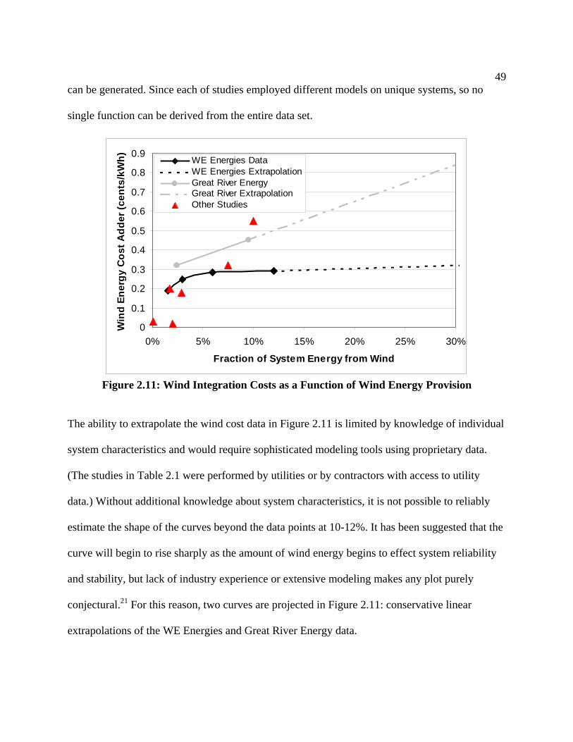
49

can be generated. Since each of studies employed different models on unique systems, so no

single function can be derived from the entire data set.

0

0.1

0.2

0.3

0.4

0.5

0.6

0.7

0.8

0.9

0% 5% 10% 15% 20% 25% 30%

Fraction of System Energy from Wind

Win

d En

ergy

Cos

t Add

er (c

ents

/kW

h) WE Energies DataWE Energies ExtrapolationGreat River EnergyGreat River ExtrapolationOther Studies

Figure 2.11: Wind Integration Costs as a Function of Wind Energy Provision

The ability to extrapolate the wind cost data in Figure 2.11 is limited by knowledge of individual

system characteristics and would require sophisticated modeling tools using proprietary data.

(The studies in Table 2.1 were performed by utilities or by contractors with access to utility

data.) Without additional knowledge about system characteristics, it is not possible to reliably

estimate the shape of the curves beyond the data points at 10-12%. It has been suggested that the

curve will begin to rise sharply as the amount of wind energy begins to effect system reliability

and stability, but lack of industry experience or extensive modeling makes any plot purely

conjectural.21 For this reason, two curves are projected in Figure 2.11: conservative linear

extrapolations of the WE Energies and Great River Energy data.

50

With these caveats in mind, the total cost of wind energy without energy storage is estimated

by adding the intermittency cost values in Figure 2.11 to the wind curtailment costs in Figure

2.6. Figure 2.12 shows the results, based on two scenarios. The first “flexible case” uses the

lower cost system data from Figure 2.7 and the lower integration costs estimated by WE

Energies. The second “inflexible system” uses higher cost system data from Figure 2.7, and the

higher integration costs estimated Great River Energy. These two curves create an envelope of

likely marginal wind energy costs, although neither curve is a worst or best case, given the

uncertainties and limits of this model.

4.00

4.25

4.50

4.75

5.00

5.255.50

5.75

6.00

6.25

6.50

6.75

7.00

0% 5% 10% 15% 20% 25% 30% 35% 40%

Fraction Total Energy from Wind

Mar

gina

l Win

d En

ergy

Cos

t (ce

nts/

kWh)

Inflexible SystemFlexible System2 cent breakeven1.5 cent breakeven

Figure 2.12: Wind Energy Cost as a Function of Energy Penetration

Figure 2.12 provides a measure of the economic impact of wind intermittency when deployed

without storage. Unlike traditional energy sources, the cost of adding wind energy to a system

depends highly on the nature of the system, reflected in the cost envelope in Figure 2.12. Exact

quantification of the cost, or the rate of cost increase depends on many variables, but it is clear

51

that there is a substantial increase in wind energy cost at system penetration as low as 15% of

total energy from wind. This rapid rise in cost decreases the economic competitiveness of wind

energy, a situation that can be partially mitigated with energy storage. Economic considerations

will require the use of energy storage if wind is to provide an amount of electrical energy equal

to other generation sources, such as fossil, nuclear, or hydroelectric generation, each of which

often contributes greater than 50% of a region’s electrical energy demand.

2.2 Wind energy and the Need for Transmission

Long distance transmission is another enabling technology for wind energy. In some cases,

transmission may provide an alternative to energy storage to increase the amount of wind energy

that can be used in an electric power system. Regional trade of wind energy allows various

utilities to increase the overall flexibility of the electric power system, increasing economic use

of wind energy even without storage. Transmission also increases spatial diversity of wind

energy resources, and greater capacity credit. The most significant use of long distance

transmission will likely be in connecting areas with large wind resources to major load centers.

2.2.1 Benefits of Intra-regional Trade Enabled by Transmission

The various models described in section 2.1 all ignore the ability of a region to import and export

power as a method of increasing wind energy penetration. Intra-regional trade of energy may

allow some regions to increase their use of wind energy. This is particularly beneficial when

systems with different technical characteristics can be connected. An example would be

connecting a region with large amounts of hydro resources, but poor wind resources, with an

area with large amounts of inflexible coal or nuclear generation and good wind resources.

52

The use of import/export capacity should be examined critically, however, if wind energy is to

be deployed on a large scale, and not in isolated regions as it is currently used in the U.S. The

use of transmission as a method of addressing intermittency may leads to erroneous conclusions

about the ability to wind energy to economically serve load. Denmark is commonly cited as an

example of the ability of wind to serve a large fraction of a regions energy supply, with the

nation deriving roughly 15% of its electrical energy from wind generation in 2002.22 This high

level of wind energy use is partially enabled by Denmark’s large import/export transmission

capacity to Germany, Sweden, and Norway. Norway provides particular benefits because its

electric power system is based primarily on large scale hydro systems with built-in storage.23 If

this export/import capacity was reduced, this would increase operational burdens on the Danish

power system, increasing costs, and possibly requiring energy storage. Export/import

transmission capacity can be effectively reduced if surrounding regions derive a large amount of

electrical energy from wind power.

2.2.2 Benefits of Increased Spatial Diversity and Capacity Credit

Capacity credit describes the reliability of an electric generator to be able to provide energy on

demand. A typical fossil or nuclear generator can be scheduled well in advance to be available

when needed. As an example, a fossil generation plant may have a 97% chance of being

available when needed, so a 100 MW plant would have a capacity credit of 97 MW. Wind

turbines cannot be relied on to have performance anywhere close to this level of reliability. The

actual capacity credit that should be applied to wind generation is an active area of research, but

many utilities currently assign a very low or zero capacity credit to individual turbines.24 The use

of very low capacity credit for turbines is partially based on a common utility measure of

53

reliability, which is generator availability under peak load conditions, typically hot summer

days. Unfortunately, wind turbine generation in many parts of the U.S. is well below average

under these conditions, which reinforces current negative attitudes regarding the capacity credit

of wind turbines. Utilities regard wind energy almost exclusively as a mechanism to meet

renewable portfolio standards, receive tax benefits, or decrease overall fuel consumption and

emissions from load-following plants.

A highly developed transmission network could link highly diverse wind energy resources,

resulting in decreased intermittency impacts of wind energy and increased capacity credit.25

Research has demonstrated a non-zero capacity credit for wind generators that are spatially

diverse, meaning wind turbines may have the ability to offset traditional baseload generation.26 If

the capacity credit of spatially diverse wind turbines is high enough to offset generation capacity,

this could increase wind energy use by effectively shifting the “minimum baseload production”

in Figure 2.6 downward. This could effectively increase the economic use of wind energy, even

without storage, by decreasing the amount of “must run” capacity required in the system. As a

result, transmission provides a potentially more economic alternative to storage in certain

circumstances.

2.2.3 Access to Wind Resources Enabled by Transmission

Potentially the most important reason for increased transmission capacity is to provide access to

the vast untapped resources of wind energy in the Midwestern U.S. The need for long distance

transmission for renewable energy is demonstrated by a map of wind energy resources currently

considered economically exploitable, provided in Figure 2.13.

54

Figure 2.13:Distribution of Economic U.S. Wind Resources 27

Areas with class 4 or better are the most economically competitive for development of wind

energy, but some class 3 resources are being developed. This map shows that the major low-cost

wind resources are located in the upper Midwest and Rocky Mountain states. The areas that are

most compatible with very large scale wind energy deployment, in terms low population density

and limited impact on scenic areas, include northwestern Iowa, western Minnesota, and the

Dakotas.

Wind resources in the upper Midwestern U.S. have the theoretical potential to provide most of

the entire 2003 U.S. electricity demand, in terms of energy.28 In 2003, a total of about 1200 MW

55

of wind energy was in operation in the region, which produced only about 0.1% of the nations

electricity supply.29 Unfortunately, this region is extremely constrained in its ability to export

power.30 Significant transmission upgrades will be required if the U.S. is to tap into its

significant reserves of wind energy located in the upper Midwest.

2.3 The Need for Enabling Technologies to Achieve National Wind Energy Goals The basic analysis performed in sections 2.1 and 2.2 can be used to provide a “big picture”

viewpoint of possible wind energy utilization in large regions of the U.S., or in the nation as a

whole. It is not overly simplistic to claim that wind energy is currently the only renewable

energy technology economically competitive with coal and nuclear power, and that renewable

energy proponents have placed great expectations upon this technology capturing a significant

share of U.S. electricity generation.31 It is useful then to evaluate the fraction of the nation’s

electrical energy that can be met with wind energy with and without enabling technologies.

A simple regional model was developed to evaluate the need for both energy storage, and

transmission, in the context of meeting specific national goals for the use of wind energy. The

model divides the country into five regions, based on their proximity to areas with good wind

resources. Figure 2.14 provides a map of the U.S., divided into these 5 resource regions.

Additional details are provided in Appendix A.

56

Region 1 Up to 15% Energy from Wind


Region 4 No Economic Wind Resources



Figure 2.14: Wind Resource Regions Used to Evaluate the Potential Use of Wind Energy in

the U.S.

Region 1 includes far western and southwestern states. These states have good wind resources,

but in the case of Oregon and Washington, they are located in the eastern part of the states, with

little transmission. Texas also has excellent wind resources, but they are concentrated in the

western part of the state where there is little population and limited transmission.

Region 2 includes remaining western and many midwestern states. Each of these states has very

large wind resources, and in most cases could produce wind energy exceeding their demand.

Region 3 includes four midwestern states with moderate wind energy resources.

Region 4 includes southeastern states with virtually no exploitable wind resources.

Region 5 includes all remaining eastern states. Many of these states have considerable wind

energy resources, but it is unclear how much of the actual wind potential can be exploited in

these densely populated areas.

57

This model assumes that all regions except Region 2 are ultimately constrained in their ability to

meet electrical energy demand using wind generation due to resource and siting limitations. As a

result, achieving a large national wind energy goal may rely on large utilization of wind energy

in Region 2. The goal of this model was to determine the fraction of electrical energy supplied by

wind in Region 2 necessary to meet a range of possible national wind energy goals. This value

can be compared to the amount of energy that can be economically supplied without the use of

energy storage.

The model is described by the relationship

2

553311USUS2 D

)DFDF DF(DFF

++−= (2.3)

where F is the fraction of the regions electricity demand met by wind energy and D is the total

annual electrical energy demand in each region in year 2001.32 This simple model holds demand

in each region constant. Subscripts indicate regions where US represents the entire U.S. The

values for F1, F3, and F5 are determined by the wind energy resource constraints in each of the

three regions, while FUS is the desired goal for national wind energy use.

Two scenarios were evaluated. The first “transmission constrained” scenario considers limited

transmission system expansion, which limits bulk transfers of power from the Midwest to the

eastern states or far western states. In this scenario, each region relies mostly on its own wind

energy resources. Figure 2.15 shows the results with three possible curves, representing the

“aggressiveness” of wind deployment in Regions 1, 3, and 5. The low wind curve represents 0%

58

wind energy in Region 5, with 2% in Regions 1 and 3. The medium wind curve represents 2%

in Region 5 and 8% in Regions 1 and 3. This number represents a fairly aggressive but possible

target, given the limitations on land use, particularly on the east coast. The high wind curve

represents 5% wind energy in Region 5 and 15% in Regions 1 and 3.

0%

10%

20%

30%

40%

50%

60%

70%

80%

90%

100%

0% 5% 10% 15% 20% 25%

National Wind Energy Goal (Fraction of Total Electricity Supply)

Frac

tion

of R

egio

n 2

Elec

trici

ty

Supp

lied

by W

ind

Low WindMedium WindHigh Wind

Figure 2.15: Region 2 Wind Requirements to Meet National Wind Energy Goals with

Transmission Constraints In all cases, the values chosen for F in the resource constrained regions are not considered

definitive, but represent a fairly reasonable range of values, perhaps generous considering likely

opposition to wind siting in scenic and populated areas in the various regions. These values in

the high wind case are very aggressive, particularly for the east coast where the 5% target would

require about 27,000 MW of wind energy generation, compared to an installed base in 2003 of

only about 257 MW. This development would likely require extensive use of offshore wind

resources in the Atlantic, as well as controversial deployment in the eastern mountains. An

example of the challenges faced in deploying this amount of wind energy is the proposed 420

MW Cape Wind project, planned for Nantucket Sound off the coast of Massachusetts, which

faces considerable local opposition.33 The high wind case would also require substantial

transmission expansion, especially in the West and Southwest.

59

Appendix A provides additional details about the model parameters, which can be used to

generate curves for any desired values of F and D for the various regions.

Assuming the medium wind deployment is realistic, achieving a national wind energy goal of

10% would require about 60% of the electricity in Region 2 to be derived from wind, an amount

that would require extensive use of energy storage. Even if 100% of the electrical energy in

Region 2 was derived from wind energy, wind would not equal nuclear power (about 20% of

U.S. energy supply) under the very aggressive “high wind” scenario.

Figure 2.16 considers a second scenario, which substantially increases transmission export

capacity out of the high wind regions. It considers a large scale, coordinated building effort, of

10-15 new very high capacity long distance power lines, which could carry energy out of region

2 to major load centers within 1000 km of significant wind energy resources, such as eastern

Missouri, Northern Illinois, East Texas, and the Pacific Northwest. These lines could carry up to

about 30 GW, equal to the capacity of 30 large baseload power plants. This new transmission

capacity is coupled to wind generation using storage, to increase its effective capacity factor to

75%, a value which is based on models developed in Chapter 6. This is an aggressive building

plan, considering there are only four such major long distance “export” transmission lines in the

U.S., and new transmission lines are difficult to complete due in part to strong local opposition.

However, it is assumed that the perceived environmental benefits of these projects, which would

deliver an amount of energy equal to about 6% of the 2001 U.S. electricity demand, would allow

this scenario to be possible. The curves in Figure 2.16 are based on equation 2.3, but where DUS

60

is reduced by the amount generated by the export capacity. All other resource constraints in

this scenario are the same.

0%

10%

20%

30%

40%

50%

60%

70%

80%

90%

100%

0% 5% 10% 15% 20% 25%

National Wind Energy Goal (Fraction of Total Electricity Supply)

Frac

tion

of R

egio

n 2

Elec

trici

ty

Supp

lied

by W

ind

Low WindMedium WindHigh Wind

Figure 2.16: Region 2 Wind Requirements to Meet National Wind Energy Goals with New

Transmission and Storage Capacity

The increased transmission/storage scenario increases the ability of wind to meet a larger

fraction of the U.S. energy supply, although achieving a national share equal to 20% would

require more than 60% of the electricity in Region 2 to be produced by wind generation, even in

the “high wind” scenario. Regardless of what specific target is desired, it is clear that both energy

storage AND new transmission capacity will be required to meet large scale national goals for

the deployment of wind energy in the U.S.

2.4 The Benefits of Energy Storage to Solar PV Generated Electricity

Solar photovoltaic (PV) generation has the advantage of being a distributed generation source,

generating energy at the point of demand, which potentially reduces the transmission and

distribution requirements. Solar PV is also cited as a valuable source of peaking power, with

generation occurring when electricity is needed most, and most expensive. A simple analysis

61

demonstrates that for solar PV to be significant in reducing the need for peaking power

capacity, storage will be required.

PV generation without storage is limited in its ability to offset traditional peaking power

generation for two reasons. First, solar generation peak and electricity demand peak are non-

coincident by several hours. Second, solar electricity generation can experience rapid swings in

output due to weather phenomenon, such as passing clouds. Distributed PV generation would

limit the effects of such events, but a high concentration of solar PV deployed in a relatively

compact area could produce relatively large changes in output that would have to be addressed

with increased spinning reserves, or energy storage.

The potential benefits of energy storage to PV generation can be observed by comparing PV

generation to electricity demand on an hourly basis. A number of PV units have been installed on

schools in Madison, Wisconsin, and historical data in 15-minute increments is available on the

Internet.34 Figure 2.17 shows the output from two of these individual PV units, along with the

combined total output data from five separate sites. The data is for the first week of July 2002.

Each PV unit is rated at about 2 kW at peak output.

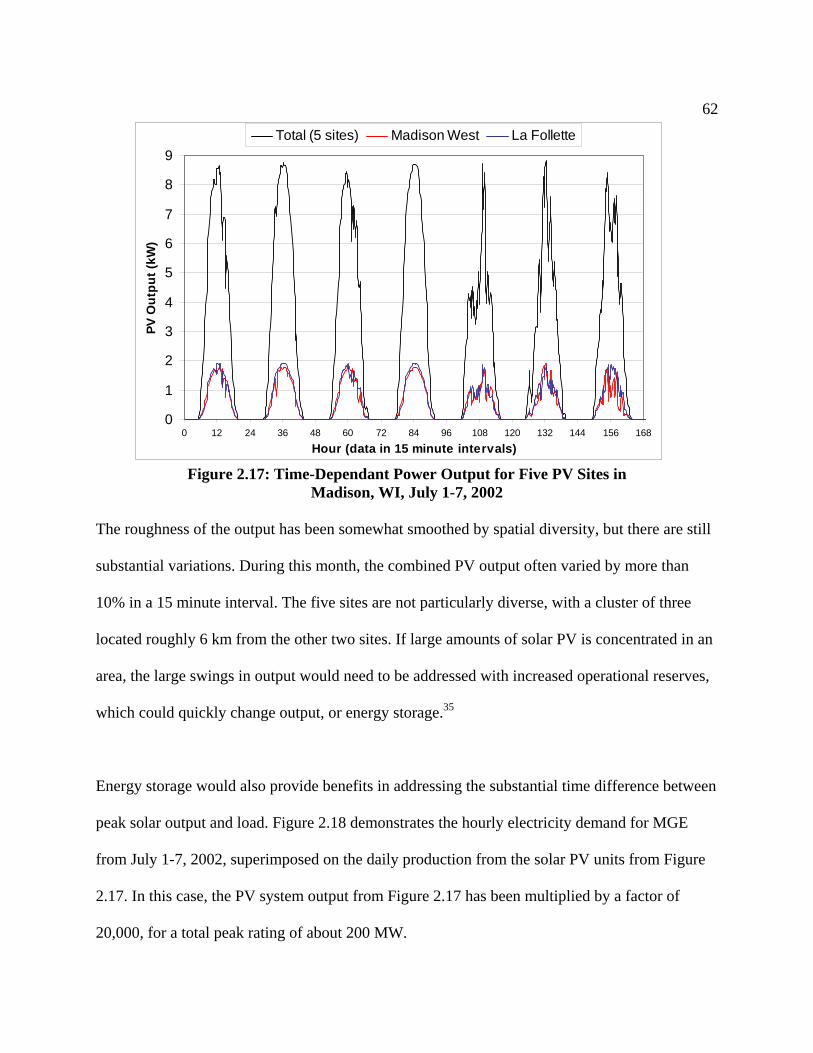
62

0

1

2

3

4

5

6

7

8

9

0 12 24 36 48 60 72 84 96 108 120 132 144 156 168

Hour (data in 15 minute intervals)

PV O

utpu

t (kW

)Total (5 sites) Madison West La Follette

Figure 2.17: Time-Dependant Power Output for Five PV Sites in

Madison, WI, July 1-7, 2002 The roughness of the output has been somewhat smoothed by spatial diversity, but there are still

substantial variations. During this month, the combined PV output often varied by more than

10% in a 15 minute interval. The five sites are not particularly diverse, with a cluster of three

located roughly 6 km from the other two sites. If large amounts of solar PV is concentrated in an

area, the large swings in output would need to be addressed with increased operational reserves,

which could quickly change output, or energy storage.35

Energy storage would also provide benefits in addressing the substantial time difference between

peak solar output and load. Figure 2.18 demonstrates the hourly electricity demand for MGE

from July 1-7, 2002, superimposed on the daily production from the solar PV units from Figure

2.17. In this case, the PV system output from Figure 2.17 has been multiplied by a factor of

20,000, for a total peak rating of about 200 MW.

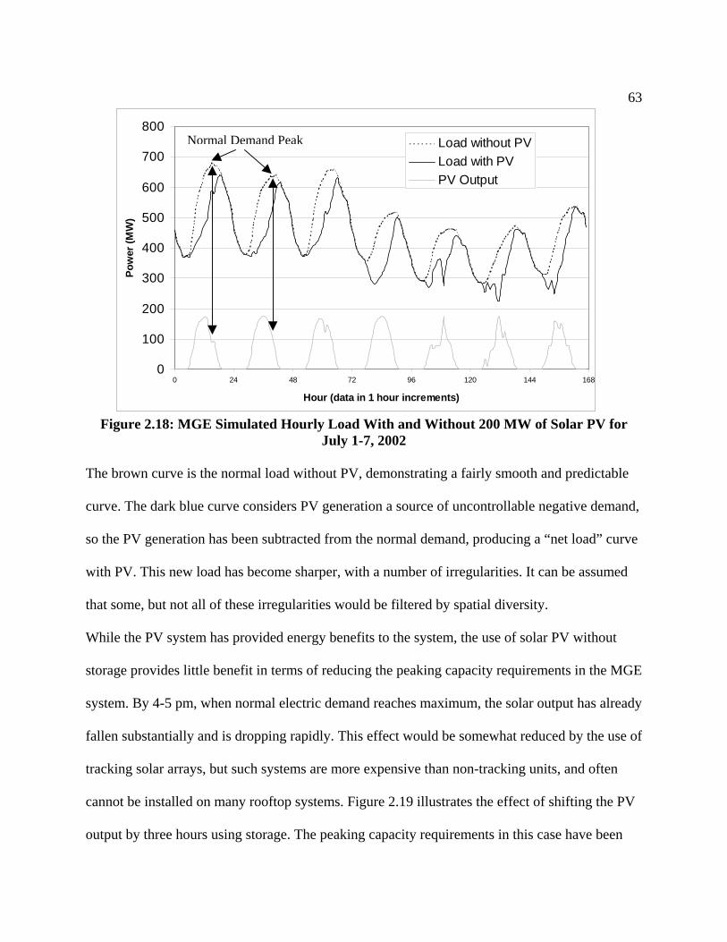
63

0

100

200

300

400

500

600

700

800

0

Pow

er (M

W)

Load without PV

Figure 2.18: M

The brown curve

curve. The dark b

so the PV genera

with PV. This ne

that some, but no

While the PV sys

storage provides

system. By 4-5 p

fallen substantial

tracking solar arr

cannot be installe

output by three h

Normal Demand Peak

24 48 72 96 120 144 168

Hour (data in 1 hour increments)

Load with PVPV Output

GE Simulated Hourly Load With and Without 200 MW of Solar PV for

July 1-7, 2002

is the normal load without PV, demonstrating a fairly smooth and predictable

lue curve considers PV generation a source of uncontrollable negative demand,

tion has been subtracted from the normal demand, producing a “net load” curve

w load has become sharper, with a number of irregularities. It can be assumed

t all of these irregularities would be filtered by spatial diversity.

tem has provided energy benefits to the system, the use of solar PV without

little benefit in terms of reducing the peaking capacity requirements in the MGE

m, when normal electric demand reaches maximum, the solar output has already

ly and is dropping rapidly. This effect would be somewhat reduced by the use of

ays, but such systems are more expensive than non-tracking units, and often

d on many rooftop systems. Figure 2.19 illustrates the effect of shifting the PV

ours using storage. The peaking capacity requirements in this case have been

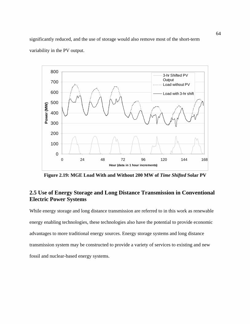
64

significantly reduced, and the use of storage would also remove most of the short-term

variability in the PV output.

0

100

200

300

400

500

600

700

800

0 24 48 72 96 120 144 1Hour (data in 1 hour increments)

Pow

er (M

W)

68

3-hr Shifted PVOutputLoad without PV

Load with 3-hr shift

Figure 2.19: MGE Load With and Without 200 MW of Time Shifted Solar PV

2.5 Use of Energy Storage and Long Distance Transmission in Conventional Electric Power Systems While energy storage and long distance transmission are referred to in this work as renewable

energy enabling technologies, these technologies also have the potential to provide economic

advantages to more traditional energy sources. Energy storage systems and long distance

transmission system may be constructed to provide a variety of services to existing and new

fossil and nuclear-based energy systems.

65

2.5.1 Benefits of Energy Storage to Traditional Generation Sources

Most energy is stored in the form of primary fuels such as coal, uranium or water, and converted

into electrical energy on demand. Limitations in the economic and technical ability and of

generators to quickly convert primary fuel into electricity has motivated the use of energy

storage long before large-scale renewable energy systems were considered. Energy storage can

provide three general categories of services to electric power systems:

1) Provision of demand responsive energy. Energy storage can respond rapidly to variations

in demand, by both producing electricity on demand, and “absorbing” excess supply.

This ability creates a number of opportunities to couple energy storage with traditional

sources. First, it can decrease cycling of baseload coal units, increasing their efficiency

and decreasing their O&M costs. Second it replaces natural gas and petroleum with lower

cost coal and uranium for peaking fuels. Nuclear generated electricity particularly

benefits from this application due to its limited cycling ability.

2) Reserves. Energy storage systems are often superior for providing power reserves. They

can generally respond to rapid swings in demand, without the cost associated with

partially loaded boilers or turbines. Most pumped hydro facilities represent a significant

source of spinning reserve, and several large batteries have been constructed primarily to

provide spinning reserve. Energy storage can also provide standby reserves or “black

start” capacity for large power plants that is typically provided by large diesel generators

or gas turbines.

3) Distribution of generation and transmission resources. Energy storage systems can

replace electricity generation in areas where generation would be difficult to build for a

variety of reasons. It can also provide an alternative to increased transmission capacity.

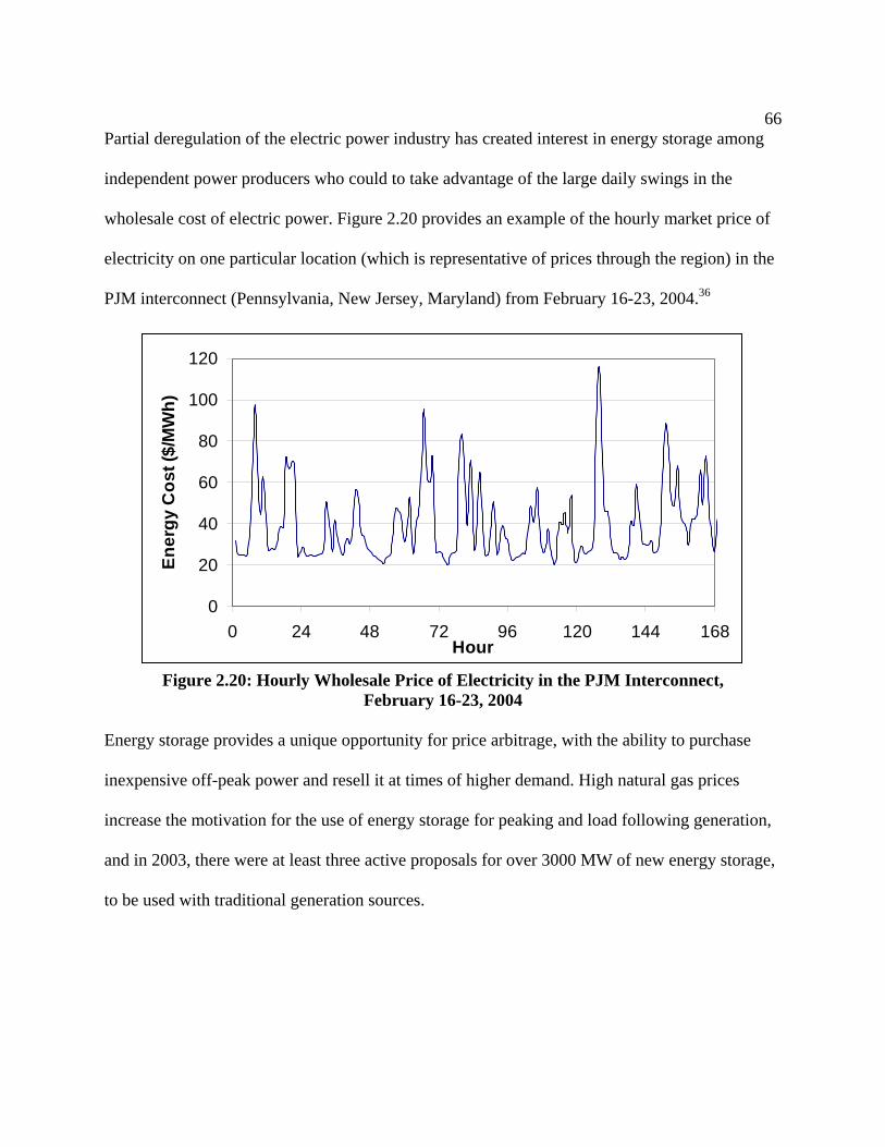
66

Partial deregulation of the electric power industry has created interest in energy storage among

independent power producers who could to take advantage of the large daily swings in the

wholesale cost of electric power. Figure 2.20 provides an example of the hourly market price of

electricity on one particular location (which is representative of prices through the region) in the

PJM interconnect (Pennsylvania, New Jersey, Maryland) from February 16-23, 2004.36

0

20

40

60

80

100

120

0 24 48 72 96 120 144 168Hour

Ener

gy C

ost (

$/M

Wh)

Figure 2.20: Hourly Wholesale Price of Electricity in the PJM Interconnect,

February 16-23, 2004

Energy storage provides a unique opportunity for price arbitrage, with the ability to purchase

inexpensive off-peak power and resell it at times of higher demand. High natural gas prices

increase the motivation for the use of energy storage for peaking and load following generation,

and in 2003, there were at least three active proposals for over 3000 MW of new energy storage,

to be used with traditional generation sources.

67

2.5.2 Long Distance Transmission

Long distance transmission enables the use of three general classes of electricity production

technologies, based on the fuel source: fuels that cannot be moved for technical reasons, such as

hydro and wind power; fuels that cannot moved for economic reasons, such as low density

lignite coal; and fuels that be cannot moved for social or policy reasons, such as the use of coal

in southern California. Since coal (especially lignite coal) is relatively expensive to transport,

and difficult to site in populated areas, several long distance “coal by wire” transmission lines

have been constructed in the U.S., with additional projects being actively pursued.37,38 Long

distance transmission enables otherwise uneconomic coal resources to be effectively integrated

into the electric power system.

2.6 Conclusions

The majority of the electric power used in the U.S. is provided by baseload energy sources. Most

of this baseload energy is derived from sources considered by many to be environmentally

harmful. Wind energy is currently the only renewable energy source capable of providing

competitively priced baseload energy. Yet without enabling technologies, including storage and

transmission, wind is only capable of economically providing a relatively small fraction of the

nation’s electrical energy requirements. It is likely that large-scale deployment of wind energy

systems in the U.S. will require the extensive development of new long distance transmission

and energy storage.

Even without large-scale deployment of renewable energy, new development of transmission and

energy storage is likely, given its benefits to traditional systems. For these reasons, it is important

68

to examine the various environmental consequences of deployment of energy storage and

transmission technologies used with both renewable and traditional energy sources.


1 Federal Energy Regulatory Commission Via http://www.ferc.gov/docs-filing/eforms/form-714/data/2001/01MAIN.EXE Accessed November 2, 2003.

2 Gellings, C. W., Ed. (1996). Demand Forecasting in the Electric Utility Industry, Pennwell

Publishing Co. 3 Federal Energy Regulatory Commission Via http://www.ferc.gov/docs-filing/eforms/form-

714/data/2002/MAIN3.EXE Accessed March 1, 2004. 4 Federal Energy Regulatory Commission. FERC 714 data for 2002 for the following regions:

WSCC, PJM, ERCOT, WEPCO, MGE, MAPP, NE ISO. Via http://www.ferc.gov/docs-filing/eforms/form-714/data.asp.

5 United States. Dept. of Energy. Office of Utility Technologies. and Electric Power Research

Institute. (1997). Renewable energy technology characterizations. Pleasant Hill, CA. 6 Yih-huei Wan (2003) National Renewable Energy Laboratory. Personal Communications.

October 20 – December 2, 2003. 7 Wisconsin Energy Corporations 2002 Performance Report. Available at http://www.wec-performancereport.com/pdf/env/env_renewable.pdf. 8 Hirst, E. (2001). Interaction of Wind Farms with Bulk-power operation and Markets. Project

for Sustainable FERC Energy Policy. Alexandria, Virginia. 9 Cavallo, A. J. (1995). High-Capacity Factor Wind Energy Systems. Journal of Solar Energy

Engineering 117: pp. 137-143. 10 Denny, F. I. and D. E. Dismukes (2002). Power System Operations and Electricity Markets,

CRC Press. 11 Termuehlen, H. and W. Emsperger (2003). Clean and Efficient Coal-Fired Power Plants. New

York, ASME Press. 12 Hirst, E. (2001). Real-Time Balancing Operations and Markets: Key to Competitive Wholesale

Electricity Markets. Edison Electric Institute and Project for Sustainable FERC Energy Policy. 13 Milligan, M. R., et al. (1995). Estimating the Economic Value of Wind Forecasting to Utilities.

Windpower '95, Washington, D.C.

69

14 Hirst, E. (2001). Interaction of Wind Farms with Bulk-power operation and Markets. 15 Brooks, D. L., et al. (2002). Assessing the Impact of Wind Generation on System Operations at

Xcel Energy – North and Bonneville Power Administration. Electrotek Concepts, Inc. Available at http://www.uwig.org/opimpactspaper.pdf.

16 Dragoon, K. and M. Milligan (2003). Assessing Wind Integration Costs with Dispatch Models:

Case Study of PacifiCorp. National Renewable Energy Laboratory. NREL/CP-500-34022. 17 Hirst, E. (2002). Integrating Wind Energy with the BPA Power System: Preliminary Study.

Bonneville Power Administration. Portland, OR. 18 Electrotek Concepts, Inc. (2003). We Energies System Operations Impacts of Wind Generation

Integration Study. We Energies. ETK-2044. 19 Kirby, B., et al. (2003). California Renewables Portfolio Standard: Renewable Generation

Integration Cost Analysis, Phase I: One Year Analysis of Existing Resources Results and Recommendations, Final Report. California Wind Energy Collaborative. CWEC-2003-06.

20 Seck, T. (2003). GRE Wind Integration Study. UWIG Technical Wind Workshop. 21 Yih-huei Wan (2003) National Renewable Energy Laboratory. Personal Communication.

February 17, 2004. 22 Lund, H. and E. Munster (2003). Modeling of energy systems with a high percentage of CHP

and wind power. Renewable Energy 28(14): pp. 2179-2193. 23 Lund, H. and E. Munster (2003). Management of surplus electricity-production from a

fluctuating renewable-energy source. Applied Energy 76(1-3): pp. 65-74. 24 Milligan, M., et al. (2002). Wind Energy and Power System Operations: A Survey of Current

Research and Regulatory Actions. The Electricity Journal 15(2): pp. 56-67. 25 Archer, C. L. and M. Z. Jacobson (2003). Spatial and temporal distributions of U.S. winds and

wind power at 80 m derived from measurements. Journal of Geophysical Research 108(D9): pp. 4289.

26 Milligan, M. R. (2002). Modeling Utility-Scale Wind Power Plants, Part 2: Capacity Credit.

National Renewable Energy Laboratory. Golden, Colorado. NREL/TP-500-29701. 27 Elliott, D. L., et al. (1987). Wind Energy Resource Atlas of the United States. Solar Energy

Research Institute. Golden, CO. DOE/CH 10093-4

70

28 Petersik, T. (1999). Modeling the Costs of U.S. Wind Supply. Issues in Midterm Analysis and

Forecasting. U.S. Department of Energy. Washington D.C. DOE/EIA-0607(99). 29 American Wind Energy Association Via http://www.awea.org/projects/ Accessed May 01,

2004. 30 Wisconsin Public Service Corporation. (2003) Certificate of Public Convenience and

Necessity Application. Arrowhead to Weston Transmission Project. Available at: http://psc.wi.gov/electric/cases/05ce113/document/vol1.pdf.

31 Brown, L. R. (2003). Wind Power Set to Become World's Leading Energy Source. Earth Policy

Institute. 32 U.S Department of Energy (2003). Electric Power Annual. Energy Information

Administration. Washington, DC. 33 Burkett, E. (2003). A Mighty Wind. New York Times Magazine. June 15. 34 Madison Gas & Electric Via http://www.mge.com/environment/solar/host/index.htm Accessed

February 13, 2004. 35 Rahman, S. and M. Bouzguenda (1994). A Model to Determine the Degree of Penetration and

Energy Cost of Large Scale Utility Interactive Photovoltaic Systems. IEEE Transactions on Energy Conversion 9(2): pp. 224-230.

36 PJM Interconnection (2004) Via http://www.pjm.com/markets/energy-market/real-time.html

Accessed March 3, 2004. 37 Lignite Vision 21 Program. (2004) Via http://www.lignitevision21.com/061402news.htm

Accessed March 3, 2003. 38 Black & Veatch TransAmerica Generation Grid (2004) Via

http://www2.bv.com/services/projects/pd/tagg/technical_sites.asp Accessed March 3, 2004.

71

3. Methods and Metrics

To accurately assess the environmental impact of renewable enabling technologies and to

provide a uniform comparison between these technologies and other energy supply systems, a

uniform set of metrics was derived. These metrics focus on analyzing the life-cycle

environmental impacts of each energy supply technology.

3.1 Life-Cycle Environmental Impact Assessment

The evaluation of renewable enabling technologies is based on environmental life-cycle

assessment. Life-cycle assessment (LCA) is a general accounting methodology that considers

various environmental impacts produced by a product over its lifetime.1 A typical life-cycle

analysis may consider such issues total energy use, consumption of various natural resources,

and releases of environmentally harmful waste products to air, land, and water. Each of these

impacts is measured for the construction, operation, and decommissioning of the evaluated

product. Many life-cycle analyses focus primarily on energy consumption, because

environmental impact generally proportional with energy use.

There are two basic tools used in life cycle assessment, Process Chain Analysis (PCA) and

Economic Input/Output (EIO).2 The PCA method uses material inventories and process flows to

evaluate energy usage at each stage of product manufacture and use. A complete PCA requires

knowledge of the quantity of each material (steel, plastic, etc.) in a product, and also an

understanding of the total energy and emissions associated with manufacturing each of the

72

materials. This method of life-cycle analysis also requires an understanding of the energy and

emissions involved with many different manufacturing processes.

Complete material inventories are often not available, and manufacturing data for complete

systems is often difficult to estimate. Manufacturing may require hundreds of integration steps,

some of which may be proprietary and difficult to evaluate. In many products, such as batteries

and electrical equipment, the manufacturing energy exceeds the energy required to obtain raw

materials. Economic Input/Output methods avoid such difficulties by using estimates of the

relationship between energy and the monetary value of materials and processes. The EIO method

requires an accurate accounting of purchases of energy and fuels throughout the manufacturing

process. Groups in several countries have performed this accounting across many manufacturing

sectors. In the U.S., an EIO database is currently maintained by the Green Design Initiative at

Carnegie-Mellon University that estimates energy use and emissions related to the dollar value

of 485 products and service categories, based on the U.S. Department of Commerce’s

commodity model of the U.S. economy.3 This database includes EIO data on many common

manufactured products such as metal products, structures, transportation equipment, and

chemicals.

In general, PCA assessments are more difficult, but often more accurate than EIO assessments.4

Since EIO aggregates data across entire industries, the specific product being evaluated (a

particular $20,000 automobile, for example) is likely different than the average product ($20,000

worth of automobile averaged across the entire industry). To maximize both accuracy and ease, a

hybrid-LCA approach is often used, where the majority of the product assessment uses PCA,

73

with EIO used where PCA would be too difficult, or complete information is not available.5

For example, evaluation of a wind turbine may require an estimation of the amount of energy

required to manufacture a steel tower, and an electric generator. The most accurate method of

estimating energy usage for the steel tower would be a PCA assessment using data that

establishes the relationship between the mass of a material (steel) and its embodied energy. The

generator consists of many different materials, and involves manufacturing processes that are

difficult to assess. It is far easier to estimate the embodied energy in the generator by obtaining

its monetary value, and using an EIO estimate for electrical apparatus. This study uses this

hybrid approach, with PCA used for most material assessment, and EIO used to assess system

operation and maintenance (O&M), certain manufacturing steps, and other less material-intense

activities.

3.2 Metrics for the Evaluation of Energy Storage Systems

The evaluation of energy storage systems in this study focused on their energy usage and

greenhouse gas emissions, using several different metrics: storage system efficiency, life cycle

efficiency, life-cycle greenhouse gas emission rate, and the storage system energy/power ratio.

3.2.1 Storage System Efficiency

The most important technical parameter of an energy storage system is the “round trip

efficiency,” which represents the conversion efficiency during the storage and generation cycle.

Since all storage facilities incur losses, the round trip efficiency is less than 100%. Storage

efficiency is an important environmental parameter, because losses require an increase in

primary electricity production, resulting in increased environmental impacts. The electrical AC-

74

AC roundtrip efficiency of the storage conversion process may be expressed as the storage

energy ratio (ERs), defined as:

out

ins kWh

kWhER = . (3.1)

Since the energy ratio measured by equation 3.1 is effectively the inverse of efficiency, it is

greater than 1 for all energy storage systems except CAES, which is a hybrid storage-generation

system described in Chapter 4. While the ERs reflects the losses that occur in the power

conversion stages, additional storage-related inefficiencies occur from electricity transmission

and losses that may occur over time in the storage medium.

Additional transmission losses are due to the extra “path” that electricity must travel due to the

use of storage. Figure 3.1 shows a highly simplified transmission infrastructure from generation

to load. Generation occurs at a voltage typically between 10 and 21 kVAC, which is stepped-up

to a much higher transmission voltage for maximum efficiency. The voltage is then stepped-

down (generally several times) through transmission and distribution substations before final

load. The use of energy storage requires additional transmission components, including an

additional transformer step-down and step-up stage, and the incremental transmission line “path”

that electricity must travel from generator to load.

75

Figure 3.1: Additional Transmission Components Required by Energy Storage

Storage medium losses occur due to the time-related degradation of the storage medium, such as

evaporation or seepage of water in pumped hydro reservoirs. Figure 3.2 is a generalized energy

flow diagram showing the sources of losses associated with energy storage.

Electricity Output

Electricity Output

Total Losses (Waste Heat)

Figure 3.2: Energy Flow in an Energy Storage System

The total net energy ratio, ERnet can be calculated by including transmission losses resulting from

the use of storage in addition to losses associated with the storage process.

76

ERnet = ERs · ERT · ERM (3.2)

The multipliers in equation 3.2 are ERT, which is the transmission loss multiplier and ERM,

which is the medium loss multiplier. Each of the factors in equation 3.2 are equal to or greater

than 1.

3.2.2 Life Cycle Energy Requirements and Efficiency

In addition to the electricity stored, energy is required to construct, operate, and decommission

an energy storage facility. This “embodied” energy can be considered part of the overall life-

cycle efficiency of an energy storage system. To calculate this life cycle efficiency, energy

associated with construction and operation must be assessed.

Energy associated with storage plant construction, EES, can be expressed in terms of energy per

unit of storage plant constructed (GJt/MWhe). To calculate the energy requirements of plant

construction per unit energy stored, EES must be divided by the total amount of energy stored

over the life of the plant.

Construction energy requirement per unit energy stored = LS

S

EEE P•

(3.3)

Where P is the storage plant size in MWhe and is the total amount of electrical energy

(MWh) stored over the lifetime of the storage plant.

LSE

To estimate we must know both the estimated life of the storage plant, and its annual

production rate, or capacity factor. Lifetimes of energy storage facilities are highly variable

depending on technology, and discussed in detail in Chapter 4. The maximum capacity factor (as

LSE

77

defined in section 2.1.2) of an energy storage plant is 50%, which would result in the plant

always either generating, or storing at full power. Most storage plants currently in operation have

capacity factors of 10-25%, with about 20% being typical.6

Operational energy requirements per unit of energy stored (excluding stored electricity) is

described by EEop (GJt/GWh).

The net energy requirements for each unit of electricity delivered to load by an energy storage

system can be calculated by summing the net energy ratio (equation 3.2) and the additional life

cycle energy requirements (equation 3.3 and EEop.) The inverse of this value can be expressed as

the life-cycle efficiency, . LSη

t

LS

Pη

η

•⎟⎟⎠

⎞⎜⎜⎝

⎛⎟⎟⎠

⎞⎜⎜⎝

⎛ •++

=

LS

Sopnet E

EEEEER

1 (3.4)

where ηt is the thermal to electric energy conversion efficiency, which accounts for the

difference in quality between thermal energy and electrical energy. Both EES and EEop are

expressed in terms of primary thermal energy, since the majority of energy related to

construction and operation results from the combustion of fossil fuels.7

The uniform treatment of ηt is an important limitation to the calculation of life-cycle efficiency,

and is discussed in more detail in section 3.4.

78

3.2.3 Greenhouse Gas Emissions

The life-cycle greenhouse gas emissions from electricity delivered by an energy storage facility

originate from three major sources: generation of electricity to be stored, storage plant

operations, and construction of the energy storage facility. GHG emissions are generally reported

in terms of CO2-equivalent (CO2e) emissions, and include non CO2 greenhouse gasses such as

methane (CH4) and nitrous oxide (N2O). Greenhouse gas emissions are typically reported in the

numerically equivalent terms of g/kWh, kg/MWh, or tonnes/GWh.

The life-cycle emissions rate (kg COLSEF 2e/MWh) describes the average emissions per unit of

energy delivered to the consumer by the energy storage unit. The rate is calculated in a manner

similar to the life-cycle efficiency.

Emissions related to stored electricity are a function of the emissions factor for primary

electricity generation, EFgen, and the net energy ratio, ERnet. Life-cycle emissions related to

storage plant construction may be expressed as the total construction-related emissions divided

by the lifetime output of the storage plant, similar to the life-cycle energy calculated in equation

3.3. Emissions related to plant operations are given by EFop. The complete life-cycle emissions

factor, is then defined as: LSEF

( ) ⎟⎟⎠

⎞⎜⎜⎝

⎛ •++•=

LS

Sopnetgen

LS

EEM

EFEREF EFP

(3.5)

where EMS (kg CO2e/MWhe ) is the emissions per unit of storage plant constructed.

79

3.2.4 Energy/Power Ratio

An energy storage system consists of both an energy component and a power component. The

energy component is the storage vessel, and the storage medium, which may be water, air, an

electrolyte, or some other medium. The power component is a power converter, which may be a

water or gas turbine, or a battery stack.

The energy and power components are generally independent of one another in terms of size. As

an example, a storage system may be able to deliver 50kW for 8 hours, or 400 kW for 1 hour,

both of which have identical storage capacity (400 kWh) but with different power components.

The energy/power ratio of an energy storage system is defined as the amount of time the system

can deliver full rated power. The energy/power ratio, which describes the relative size of the

energy storage and power components, is unrelated to the energy ratio (ER) described in section

3.2.1, which is a measure of storage plant efficiency. Storage facilities are designed for local

conditions and requirements, which results in substantial differences in the energy/power ratio

(MWh/MW) for different applications and different technologies. This ratio can vary from about

1 hour for power quality battery systems, to 30 hours or more for some pumped hydro facilities.8

However, most bulk energy storage facilities planned or in place are sized by economic

constraints to deliver energy during one to two 8-hour peaking loads, so the energy/power ratio is

generally between 8 and 16 hours. Variations in the energy/power ratio produces some degree of

inconsistency, since the energy storage component is a large fraction of the embodied energy,

particularly in BES systems.

80

3.2.5 Summary of Energy Storage Metrics

Using equations 3.1-3.5 we can summarize the basic values that describe the basic energy and

GHG emissions performance of any energy storage system.

ERnet: a multiplier that increases the primary electrical energy requirements and

emissions per unit of energy stored (MWhin/MWhout)

EES: the “embodied” energy associated with storage plant construction per unit of

storage required (GJt/MWhe)

EEop: the operational energy requirement per unit of energy stored and delivered by the

storage system to the load (GJt/GWhe)

EMS: the “embodied” emissions associated with storage plant construction per unit

storage required (kg CO2e/MWhe)

EFop: the operational emissions factor per unit of energy stored and delivered by the

storage system to the load (kg CO2e/MWhe)

3.3 Metrics for the Evaluation of Electricity Transmission and Distribution Systems The evaluation of transmission and distribution (T&D) systems is motivated by providing an

equitable comparison between traditional energy sources and renewable alternatives. Typically,

life-cycle analysis of electric power generation provides measures of impact at the “busbar”

representing the impact per unit electricity produced by the power plant. If the impacts of

electricity actually used are to be measured accurately, the effects of T&D must be considered.

Consideration of T&D is important for two reasons. First, T&D losses act as multipliers, not

adders, which means they tend to magnify the effects of high environmental impact sources.

Second, T&D effects are largely a function of proximity between source and load, which varies

depending on the generation technology.

81

This proximity effect is of particular importance to renewable energy sources including wind

and solar PV. For wind, the great distances between resource and load will likely mean greater

than average transmission distances, requiring greater amounts of transmission infrastructure and

losses per unit of delivered energy. For PV, generation of electricity at the load eliminates most

or all of the T&D path for generated electricity. In this case, only by adding T&D affects to

traditional sources can the full benefits of distributed sources such as solar PV be recognized.

3.3.1 T&D Loss Effects

In terms of energy use, the most significant impacts of T&D systems are due to losses that occur

between generation and load. The T&D loss rate, Ltd, is typically between 3% and 12%. Losses

in the transmission system require an increase in the system size to produce a desired output.

This multiplier effect can be written as:

tdL-1(MW)Capacity Power Delivered (MW)Capacity Power Installed = (3.6)

This multiplier effect increases both the system size (power) and the required input energy (fuel).

As an example, a LCA may evaluate the total impacts from a generator that delivers 1 MWh of

electricity to the load, at a rate of 1 MW. If the total T&D loss rate is 10%, the analysis will

actually need to consider the production of 1.11 MWh by a plant 1.11 MW in size.

3.3.2 Other T&D Life-Cycle Energy Requirements

Losses in the T&D system can be combined with the T&D construction and operation

components to derive a life-cycle energy requirement for energy delivered by an electric

generator. These additional adder terms include EEop for the T&D system, and the normalized

construction energy, which is calculated in a manner similar to equation 3.3:

82

Construction energy requirement per unit energy transmitted = Ltd

td

EEE

(3.7)

Where EEtd is the embodied energy in the T&D system, and is the amount of energy

transmitted by the T&D system over its lifetime.

LtdE

3.3.3 Greenhouse Gas Emissions Resulting from Electricity T&D

Losses from transmission and distribution, along with construction and O&M of T&D equipment

results in increased greenhouse gas emission related to electricity generation. The net emissions

resulting from electricity delivered by T&D system can be calculated using the life-cycle

components, similar to equation 3.5. This can be described by an emissions factor which

includes T&D, EFTD, (kg CO2e./MWh) given by:

⎟⎟⎠

⎞⎜⎜⎝

⎛++⎟⎟

⎠

⎞⎜⎜⎝

⎛= L

td

tdop

td

genTD E

EMEFL-1

EFEF (3.8)

where EFgen is the life-cycle GHG gas emissions factor for electricity generation.

EFop is the Emissions Factor due to operation of the T&D system.

EMtd is the embodied emissions associated with T&D system construction.

3.3.4 Application of T&D Metrics

The T&D metrics derived in this section must be applied appropriately for equitable comparison

of generation sources. For example, many analyses consider the effect of coal or nuclear

generation at the point where these plants enter the local transmission grid. A comparison

between these and a distant wind source would require adding the additional transmission

requirements to deliver the wind energy to approximately the same distance to load as the

83

nuclear or coal plant. However, comparison between PV system and any other centralized

generation facility must add on the entire T&D system to the centralized source, since the PV

system effectively includes all transmission and distribution.

3.4 Metrics for the Evaluation of Integrated Renewable Energy/Storage Systems An energy storage system may be electrically coupled to a renewable energy source to create an

energy system that is equivalent to a traditional fossil or nuclear energy source.

3.4.1 System Boundary

An integrated renewable energy system includes renewable energy generation, energy storage,

and certain transmission components.

Figure 3.3 illustrates the system boundary for a complete “dispatchable renewable” energy

system. The assessment of such a system includes the entire life cycle of the generation system,

storage system, and transmission. The elements of the energy storage sub-system are shown in

the dotted box in Figure 3.3

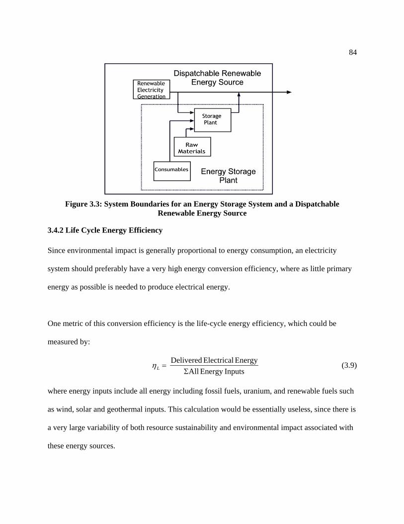
84

Figure 3.3: System Boundaries for an Energy Storage System and a Dispatchable

Renewable Energy Source

3.4.2 Life Cycle Energy Efficiency

Since environmental impact is generally proportional to energy consumption, an electricity

system should preferably have a very high energy conversion efficiency, where as little primary

energy as possible is needed to produce electrical energy.

One metric of this conversion efficiency is the life-cycle energy efficiency, which could be

measured by:

InputsEnergy AllEnergy Electrical Delivered

Σ=Lη (3.9)

where energy inputs include all energy including fossil fuels, uranium, and renewable fuels such

as wind, solar and geothermal inputs. This calculation would be essentially useless, since there is

a very large variability of both resource sustainability and environmental impact associated with

these energy sources.

85

A more valuable metric of environmental performance is the life-cycle fossil efficiency, where

only fossil energy inputs are considered in equation 3.9. This metric is useful for a number of

reasons. First life-cycle fossil fuel efficiency provides a measure of energy resource

sustainability, especially since fossil fuels account for more than 70% of electricity generation

and 85% of the total energy used in the U.S.9 In addition, fossil energy consumption is a more

accurate indicator of environmental impact than total energy consumption, since fossil energy

sources generally have much greater environmental impact than renewable energy sources.

The energy sustainability metric used in this work is defined as the fossil-fuel efficiency, or

electrical energy produced per unit of fossil thermal energy.

InputsEnergy Thermal Fossil AllOutEnergy Electrical Delivered

Σ=Lη (3.10)

This measurement is a reasonable indicator of energy sustainability, and many analyses use some

formulation of this metric. For this assessment, all primary energy is assumed to be derived from

fossil sources.

Life cycle efficiencies for conventional fossil sources are typically less than 50% and are limited

by thermal conversion processes and fuel delivery requirements. For example, a combined-cycle

gas turbine with a plant thermal efficiency of 50% has a life-cycle fuel efficiency of about 42%,

mostly due to losses in the fuel delivery system.10 The net life-cycle fossil fuel efficiency of

renewable energy systems may be substantially greater than 100%, since their fossil fuel

requirements are typically much less than their production of electrical energy.

86

A renewable energy system could have a life-cycle efficiency of less than 100% and still be

superior to a fossil based system in terms of energy resource sustainability. A unit of natural gas

energy that produces 0.4 units of electrical energy from a combustion system could alternately be

used to construct a wind energy system that, over its lifetime, delivers 0.9 units of electrical

energy. In this case the renewable system produces less energy than it takes to construct it, yet it

still produces more than twice the amount of electrical energy than would be extracted by

combustion. This example illustrates the counter-intuitive result that it may be quite reasonable

for a renewable energy system to consume more energy than it produces.

Equation 3.10 is expressed as fossil fuel efficiency, but this metric can also be applied to sources

whose input energy is derived from any input fuel mix including both conventional and

renewable fuels. In this case, ηL represents the input energy multiplier, or energy return on

investment, as each unit of energy produced by the energy system requires an amount of input

energy equal to the reciprocal of ηL. The energy inputs considered in this metric must be

measured consistently for this definition to be valuable. The energy input component can be

calculated in terms of electrical or thermal energy. Using thermal energy input is a more

meaningful measure, as it requires less estimation of thermal-electrical conversion, since greater

than 96% of the energy used in the U.S. is derived from thermal sources.11 However, the large

variations in energy source impacts makes the energy return on investment metric less useful as

an environmental performance indicator than the fossil fuel efficiency metric.12

In all cases, ηL ignores the energy content of the renewable energy inputs, and assumes that there

are no significant opportunity costs or environmental impacts associated with extracting energy

87

from renewable sources. Ignoring the energy content of renewable fuels has certain problems

and limits the relevance of ηL as a comparative metric. For example, the use of solar PV energy

incident on a rooftop may have little environmental impact, but it does incur opportunity costs,

since a solar PV array displaces the opportunity for solar water heating, an application which

may have greater environmental benefits. The use of wind energy has a variety of environmental

impacts from avian mortality,13 to possible effects on local climate.14 Significant environmental

impacts that are unique to the use of renewable fuels need to be incorporated into an appropriate

sustainability metric for accurate comparison.

In addition to ignoring the energy content of renewable fuels, there are other significant

limitations to the sustainability metric defined in equation 3.10. First, it values all fossil energy

inputs equally, with the “value” of 1 unit of natural gas energy equal to 1 unit of coal energy.

Fossil energy sources are obviously not equal in terms of economic cost, sustainability of supply,

or environmental impact. However, this variation is not nearly as great as that between fossil

and renewable energy sources.

In addition, the life-cycle metric defined by equation 3.10 does not account for the differences in

time when both input and output occur. This limitation is quite common in energy assessment;

most assessments simply sum inputs and outputs and divide, regardless of when inputs and

outputs occur.15 This scenario is not necessarily inaccurate when inputs and outputs occur in

similar time frames. For example, most emissions from coal and natural gas energy production

occur at roughly the same time the energy is put into the system. For many other systems,

88

particularly renewable energy systems, most energy and emissions are “invested” before

energy production begins.

A simplified example illustrates the potential problem in a direct comparison between systems

with time-dependant energy inputs. Two different electricity systems (fossil and renewable) may

produce 1 unit of electrical output per year over 10 years. The renewable system would require

20 units of input energy at the beginning of year 1, and no input afterward. The fossil system

would require 2 units of energy per year over the 10 year system lifetime.

Traditional LCA would claim equivalent life-cycle efficiencies of 10/20 or 50% for both

systems. An economic life-cycle analysis of these two systems would likely find a much

different result if future costs were discounted to their net present value. There are legitimate

reasons why appropriate discounting should be applied in this situation. Financial discounting

occurs for a variety of reasons, including risk of default or other financial failure. The situation

with energy systems is similar. There is a real chance that the renewable system will be

damaged or destroyed before the end of its projected lifetime. This is just one reason why time-

dependant inputs and outputs should probably be discounted.16 Most life-cycle analysis ignores

the issue of time-dependent impacts. Issues related to discounting of environmental benefits and

impacts are well understood and discussed in the field of environmental economics, but these

issues are not sufficiently addressed in the fields of life cycle analysis and energy accounting.

Despite these limitations, the metric described in equation 3.10 provides a good “first-order”

approach to understanding the comparative environmental impacts of various energy systems.

89

Equation 3.10 is most accurate when comparing generation technologies that use similar

“types” of energy inputs, such as renewable energy sources. Regardless of the limitations of the

ηL metric, however, the results often demonstrate very large differences between energy systems,

often by a factor of 10 or more. While this does not necessarily mean that one system has 10

times greater impact, it does provide an relative indicator of sustainability and environmental

impact, since energy use is generally proportional to environmental impact.

3.4.3 GHG Emission Evaluation

The life-cycle greenhouse gas (GHG) emission rate is a more easily definable indicator of

environmental performance for electric power systems. The GHG emission rate can be

calculated in a manner similar to the net energy requirement. Greenhouse gas emissions from the

initial construction of dispatchable renewable energy systems result from current reliance on

fossil fuels for manufacturing and transportation.

The life-cycle greenhouse gas emissions rate from electricity produced by a dispatchable

renewable energy system is calculated in a manner similar to the life-cycle efficiency.

Energy Electrical Delivered

EmissionsGHG EFnetΣ

= (3.11)

While equation 3.11 describes the net emission rate, it provides little insight into the origin of

emissions and their calculation. Specifically, the calculation of EFnet from a system using energy

storage requires an understanding of how much electricity is placed into storage.

The net emissions factor for a generation source using energy storage system, EFnet, is the

weighted average of the emissions of energy stored and energy not stored:

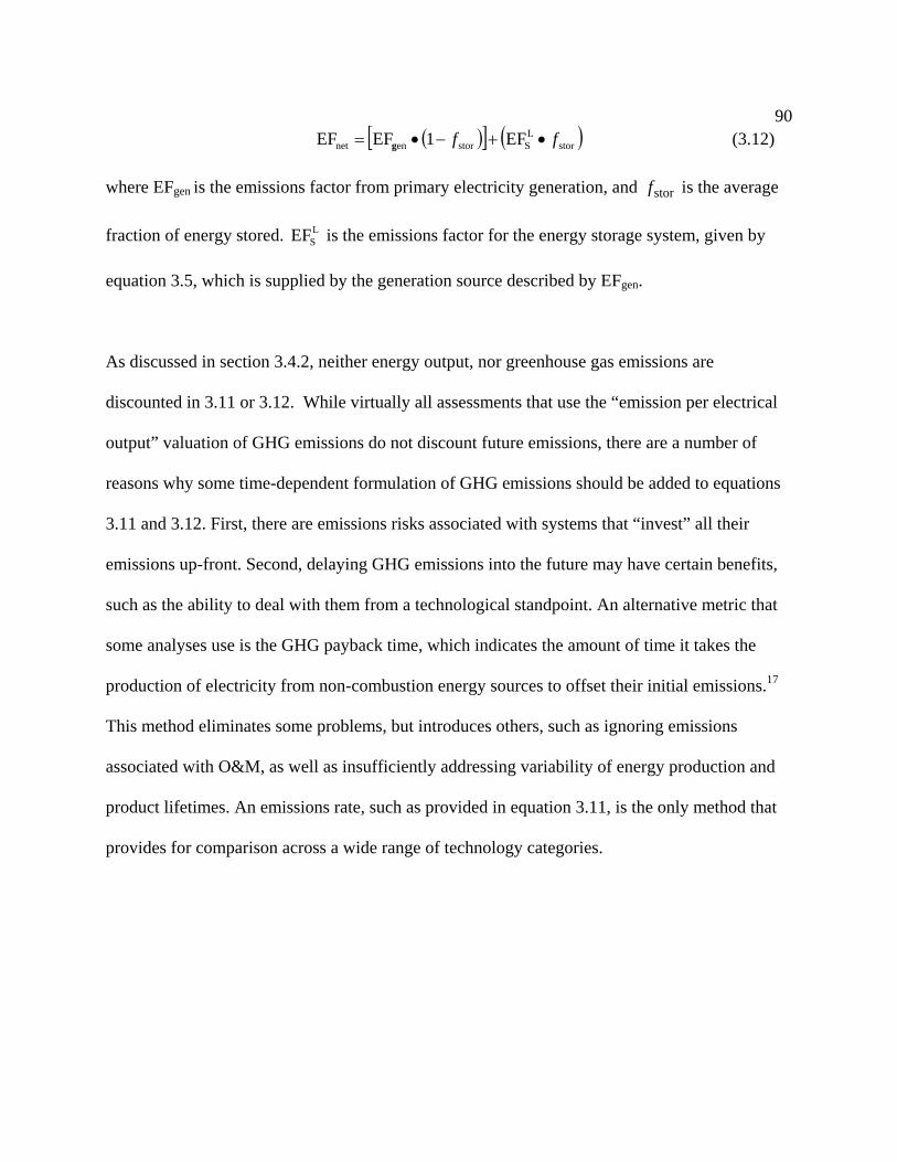
90

( )[ ] ( )storL

Sstorennet EF1EFEF ff •+−•= g (3.12)

where EFgen is the emissions factor from primary electricity generation, and is the average

fraction of energy stored. is the emissions factor for the energy storage system, given by

equation 3.5, which is supplied by the generation source described by EF

storf

LSEF

gen.

As discussed in section 3.4.2, neither energy output, nor greenhouse gas emissions are

discounted in 3.11 or 3.12. While virtually all assessments that use the “emission per electrical

output” valuation of GHG emissions do not discount future emissions, there are a number of

reasons why some time-dependent formulation of GHG emissions should be added to equations

3.11 and 3.12. First, there are emissions risks associated with systems that “invest” all their

emissions up-front. Second, delaying GHG emissions into the future may have certain benefits,

such as the ability to deal with them from a technological standpoint. An alternative metric that

some analyses use is the GHG payback time, which indicates the amount of time it takes the

production of electricity from non-combustion energy sources to offset their initial emissions.17

This method eliminates some problems, but introduces others, such as ignoring emissions

associated with O&M, as well as insufficiently addressing variability of energy production and

product lifetimes. An emissions rate, such as provided in equation 3.11, is the only method that

provides for comparison across a wide range of technology categories.

91

3.5 Metrics for the Evaluation of Storage Systems used with Fossil Energy Sources As discussed in Chapter 2, near term deployment of energy storage systems will likely be

dominated by their use with fossil energy sources. Both the fossil-fuel efficiency and GHG

emission rates described in section 3.4 can be applied to fossil/storage systems.

Potentially more important, however, is the evaluation of local or regional emissions of a variety

of air pollutants, including mercury, SO2, NOx, and particulates. The use of energy storage with

existing fossil energy sources may raise or lower these emissions, depending on how the system

is used.

The emissions rate of a pollutant X that result from the operation of an energy storage system

can be calculated in a manner similar to the life-cycle emission rate of GHG. Since most

concern regarding pollutants is regional in nature, this assessment ignores life-cycle components

such as construction and maintenance.

Calculation of this pollution emission rate is complicated by the interaction between the storage

system and the generator, as discussed in Chapter 2. As a result, the emission rate due to storage

is the product of the ERnet and the marginal emission rate of the generator, which considers the

improved efficiency of the generation plant due to the use of storage. To this must be added the

point source emission rate from the storage plant. Finally, the use of energy storage for ancillary

services, such as spinning reserve, results in a decrease in emissions. This produces a storage

emission rate of pollutant X, , defined by XSEF

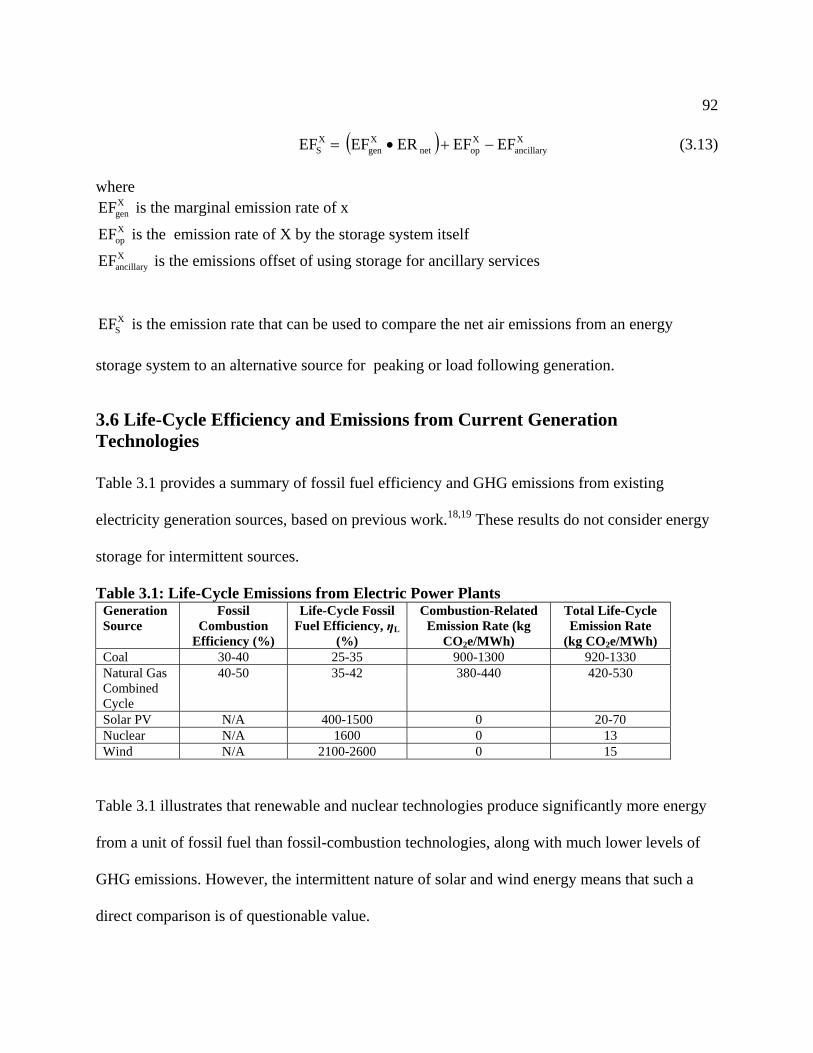
92

( ) X

ancillaryXopnet

Xgen

XS EFEFEREF EF −+•= (3.13)

where

XgenEF is the marginal emission rate of x XopEF is the emission rate of X by the storage system itself XancillaryEF is the emissions offset of using storage for ancillary services

XSEF is the emission rate that can be used to compare the net air emissions from an energy

storage system to an alternative source for peaking or load following generation.

3.6 Life-Cycle Efficiency and Emissions from Current Generation Technologies Table 3.1 provides a summary of fossil fuel efficiency and GHG emissions from existing

electricity generation sources, based on previous work.18,19 These results do not consider energy

storage for intermittent sources.

Table 3.1: Life-Cycle Emissions from Electric Power Plants Generation Source

Fossil Combustion

Efficiency (%)

Life-Cycle Fossil Fuel Efficiency, ηL

(%)

Combustion-Related Emission Rate (kg

CO2e/MWh)

Total Life-Cycle Emission Rate

(kg CO2e/MWh) Coal 30-40 25-35 900-1300 920-1330 Natural Gas Combined Cycle

40-50 35-42 380-440 420-530

Solar PV N/A 400-1500 0 20-70 Nuclear N/A 1600 0 13 Wind N/A 2100-2600 0 15

Table 3.1 illustrates that renewable and nuclear technologies produce significantly more energy

from a unit of fossil fuel than fossil-combustion technologies, along with much lower levels of

GHG emissions. However, the intermittent nature of solar and wind energy means that such a

direct comparison is of questionable value.

93

In addition to consideration of renewable intermittency, Table 3.1 also does not include the

effects of transmission and distribution. Including the effects of energy storage and T&D

provides a more equitable comparison between intermittent and dispatchable sources of electric

power. These effects are evaluated in Chapters 4-6.


1 Curran, M. A. (1996). Environmental life-cycle assessment. New York, McGraw-Hill. 2 Hendrickson, C., et al. (1997). In Comparing Two Life-Cycle Assessment Approaches: A

Process Model vs. Economic Input-Output Based Assessment. Proceedings of the 1997 International Symposium on Electronics and the Environment; Institute of Electrical and Electronics Engineers, Piscataway, NJ.

3 Green Design Initiative, Carnegie Mellon University. Via www.eiolca.net. Accessed 6/12/02. 4 Meier, P. J. (2002). Life-Cycle Assessment of Electricity Generation Systems and Applications

for Climate Change Policy Analysis, Ph.D. Dissertation, University of Wisconsin - Madison. 5 Ibid. 6 Phillips, J. (2000). Pumped storage in a deregulated environment. International Journal on

Hydropower & Dams 7(1): pp. 32-35. 7 U.S Department of Energy (2003). Annual Energy Review 2002. Energy Information

Administration, Office of Coal, Nuclear, Electric and Alternate Fuels. Washington, DC. 8 Schoenung, S. M. (2001). Characteristics and Technologies for Long- vs. Short-Term Energy

Storage: A Study by the DOE Energy Storage Systems Program. Sandia National Laboratories. SAND2001-076.

9 U.S Department of Energy (2003). 10 Spath, P. L. and M. K. Mann (2000). Life Cycle Assessment of a Natural Gas Combined-Cycle


11 U.S Department of Energy (2003). 12 Chwalowski, M. (1996). Critical Questions about the Full Fuel Cycle Analysis. Energy

Conversion & Management 37(6-8): pp. 1259-1263.

94

13 Sinclair, K. (2001). Status of Avian Research at the National Renewable Energy Laboratory.

National Renewable Energy Laboratory. Golden, CO. NREL/CP-500-30546. 14 Keith, D. W., J. F. DeCarolis, et al. The influence of large-scale wind-power on global climate.

Science. (Submitted) 15 Spreng, D. (1988). Net Energy Analysis and the Energy Requirements of Energy Systems.,

Praeger Publishers, New York. 16 Thompson, P. B. (1997). Evaluating energy efficiency investments: accounting for risk in the

discounting process. Energy Policy 25(12): pp. 989-996. 17 Tahara, K., et al. (1997). Evaluation of CO2 payback time of power plants by LCA. Energy

Conversion and Management 38: pp. S615-S620. 18 White, S. W., and G. L. Kulcinski (2000). Birth to Death Analysis of the Energy Payback

Ratio and CO2 Gas Emission Rates from Coal, Fission, Wind, and DT Fusion Electrical Power Plants. Fusion Engineering and Design 48(248): pp. 473-481.

19 Gagnon, L., et al. (2002). Life-cycle assessment of electricity generation options: The status of

research in year 2001. Energy Policy 30(14): pp. 1267-1278.

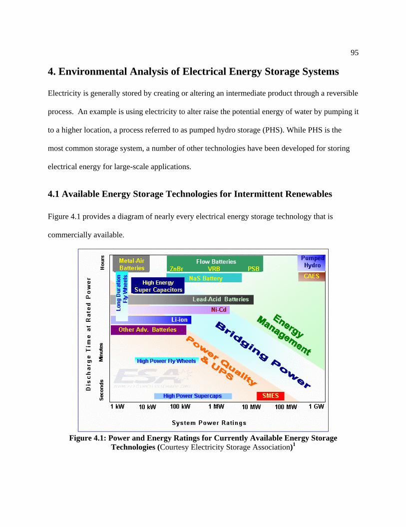
95

4. Environmental Analysis of Electrical Energy Storage Systems Electricity is generally stored by creating or altering an intermediate product through a reversible

process. An example is using electricity to alter raise the potential energy of water by pumping it

to a higher location, a process referred to as pumped hydro storage (PHS). While PHS is the

most common storage system, a number of other technologies have been developed for storing

electrical energy for large-scale applications.

4.1 Available Energy Storage Technologies for Intermittent Renewables

Figure 4.1 provides a diagram of nearly every electrical energy storage technology that is

commercially available.

Figure 4.1: Power and Energy Ratings for Currently Available Energy Storage

Technologies (Courtesy Electricity Storage Association)1

96

The x-axis in Figure 4.1 represents the system power ratings for the various energy

technologies, while the y-axis shows the amount of time the storage technology can deliver rated

power. Figure 4.1 shows three regions. In the lower left is the region of power quality and UPS

(uninterruptible power supply.) These technologies are primarily suitable for momentary

interruptions of power to end users, and currently dominated by the lead-acid battery. The upper

left hand corner also represents technologies suitable for small-scale renewable applications,

such as off-grid PV and wind system. The intermediate band is “bridging power.” This region

represents storage technologies that can deliver larger amounts of energy and power to “bridge”

the gap of large system failures. An example would be to deliver power to a commercial

building or industrial facility during a short outage. Another use is to provide “black start”

capability, or the power needed by a power plant to bring it back online. The third band, energy

management, represents large energy storage systems that can provide large amounts of power,

typically for several hours.

Since utility-scale storage of intermittent renewable sources requires both large power and

energy requirements, this study focused on technologies illustrated in the upper right hand corner

of Figure 4.1. Only three technology classes are currently economically viable for bulk energy

storage: pumped hydro storage, compressed air energy storage, and advanced batteries. While

these are the only technologies evaluated in this study, there are a number of other technologies

that may provide economic alternatives for large-scale renewable energy storage in the future.

SMES (Superconducting Magnetic Energy Storage) stores electricity in a magnetic field by

running current in loops of superconducting material. When first developed, the technology

97

looked very promising for both large scale and distributed applications, due to very high round

trip efficiencies and the potential low cost as a result of forecast improvements in materials.2

However, SMES is still burdened with high capital costs,3 and the technology is currently limited

to the niche market of “power storage,” due to its ability to deliver large amounts of power.4

SMES units are generally applied in areas of weak electric grids, with large “shock loads” of

large, sudden demand. Until there are additional fundamental breakthroughs in superconducting

materials, SMES will remain too costly for bulk power storage.

Capacitors store energy in an electric field across charged conducting plates. Capacitors are

typically used for high power, low energy applications like SMES.5 Capacitors may eventually

provide an alternative to batteries in smaller renewable storage applications currently dominated

by batteries.

Flywheels store mechanical kinetic energy by spinning a mass to a high rotational speed.

Flywheels now provide a competitive alternative to batteries in some small applications.6 While

it is unlikely that flywheels will ever be appropriate for bulk energy storage, local storage of PV

power may be a possibility for this technology.

There are two other significant energy storage technologies not shown on Figure 4.1:

Thermal energy storage describes a number of different technologies. Thermal energy storage

is often used as a load management tool by both utilities and customers to shift demand for

electricity from peak to off-peak times. An example is the production of ice or chilled water

98

during evening hours to use for cooling during peak periods. Thermal energy storage is also

used with solar thermal electricity generation, a technology not considered in this study.

Hydrogen energy storage is considered by many to be the ultimate energy storage medium, but

it can easily be disregarded in the near term due to its economic and technical limitations. The

current cost of a hydrogen energy storage system, consisting of an electrolyzer, storage tanks,

and fuel cell, is significantly greater than the cost of the other technologies evaluated.7 In

addition, it is much less efficient than the other storage technology evaluated.8 Hydrogen may be

more competitive as part as a complete storage-transmission system, an application discussed in

Chapter 5.

In the near term, pumped hydro storage (PHS), compressed-air energy storage (CAES), and

battery energy storage (BES), represent the most likely candidates for utility-scale storage

applied to renewable energy systems.

4.2 Net Energy and Emissions - Pumped Hydro Storage

Pumped hydro storage (PHS) is the most widely used form of storage, with U.S. installed

capacity exceeding 18 GW at 36 installations, and worldwide capacity exceeding 90 GW.9 PHS

stores hydraulic potential energy by pumping water from a lower reservoir to an upper reservoir.

The amount of stored energy is proportional to the height difference (head) between the upper

and lower reservoir and the volume of water stored. During periods of high demand, water is

extracted through a turbine in a manner similar to traditional hydroelectric facilities. A schematic

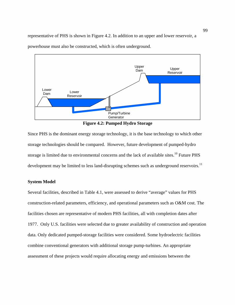
99

representative of PHS is shown in Figure 4.2. In addition to an upper and lower reservoir, a

powerhouse must also be constructed, which is often underground.

Upper Dam

Lower Dam

Pump/Turbine Generator

Upper Reservoir

Lower Reservoir

Figure 4.2: Pumped Hydro Storage

Since PHS is the dominant energy storage technology, it is the base technology to which other

storage technologies should be compared. However, future development of pumped-hydro

storage is limited due to environmental concerns and the lack of available sites.10 Future PHS

development may be limited to less land-disrupting schemes such as underground reservoirs.11

System Model

Several facilities, described in Table 4.1, were assessed to derive “average” values for PHS

construction-related parameters, efficiency, and operational parameters such as O&M cost. The

facilities chosen are representative of modern PHS facilities, all with completion dates after

1977. Only U.S. facilities were selected due to greater availability of construction and operation

data. Only dedicated pumped-storage facilities were considered. Some hydroelectric facilities

combine conventional generators with additional storage pump-turbines. An appropriate

assessment of these projects would require allocating energy and emissions between the

100

generation and storage components, as well as other tradition multi-purpose hydro uses such

as irrigation and flood control.

Table 4.1: Modern U.S. Dedicated PHS Facilities Evaluated in this Study Facility Location Completion

Date Capacity

(MW) Storage (MWh)

Bad Creek Salem, SC 1991 1000 24,000 Balsam Meadow Shaver Lake, CA 1987 200 1,600 Bath County Warm Springs, VA 1985 2,100 23,100 Clarence Cannon Center, MO 1984 31 279 Fairfield Jenkinsville, SC 1978 512 4,096 Helms Shaver Lake, CA 1984 1,206 84,000 Mt. Elbert Leadville, CO 1981 200 2,400 Raccoon Mtn. Chattanooga, TN 1978 1,530 32,130 Rocky Mtn. Armuchee, GA 1995 760 6,080

4.2.1 Plant Construction and Decommissioning

Site Preparation and Reservoir Development

Most pumped hydro projects are large in scale, with sizes often exceeding 1000 MW and

requiring construction or modification of two or more reservoirs and multiple dams. In a few

cases the lower reservoir is a river or an existing lake.

The major components of energy utilization and emissions associated with construction of PHS

dams and reservoirs include earth moving, rock quarrying, drilling and blasting, concrete

manufacturing and transport, and installation of rock fill, earth, and concrete dams.

PCA and EIO data were utilized to calculate energy and emissions for each project based on the

following parameters: amount of material moved to create reservoirs, total volume and

composition of reservoir dams, total volume of rock displaced for shafts, tunnels and

powerhouses, and the volume of installed tunnel and reservoir liners.

101

There is considerable variation in PHS projects based on diverse local topography and geological

variations. PHS dams are typically earth- or rock-fill, which require substantially less

construction energy than concrete dams.

Capital Equipment

Most of the capital equipment associated with PHS is the electrical system, including pump-

turbines and motor-generator sets, as well as transformers, switchgear, and transmission systems.

EIO data and capital equipment costs12 were used to estimate total energy and GHG emissions.

Reservoir Carbon Emissions

The development of hydroelectric reservoirs can result in considerable GHG emissions.13

Biomass cleared from the land prior to the construction of the reservoir creates a net increase in

atmospheric carbon. In addition, flooded biomass decays both aerobically, producing carbon

dioxide, and anaerobically, producing both CO2 and methane. The amount of GHG generated

depends on reservoir size, previous vegetation, and climate. The science of reservoir GHG

emissions is relatively recent and includes many uncertainties related to methane production.14

PHS development generally involves clearing and tree removal in a large percentage of the

reservoir area, so this assessment assumes carbon emissions will result from the aerobic decay of

biomass based on reservoir size. The GHG emissions associated with reservoir creation are a

significant, but largely “reversible” source, since the reservoirs can be drained and replanted.

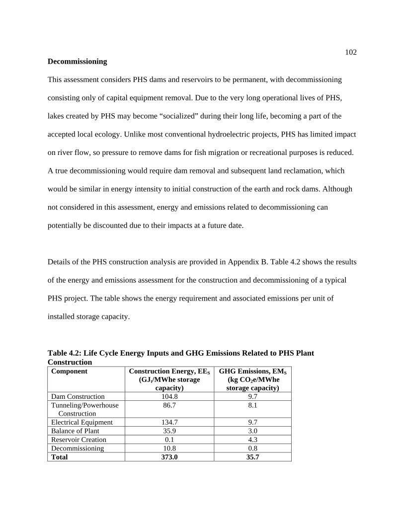
102

Decommissioning

This assessment considers PHS dams and reservoirs to be permanent, with decommissioning

consisting only of capital equipment removal. Due to the very long operational lives of PHS,

lakes created by PHS may become “socialized” during their long life, becoming a part of the

accepted local ecology. Unlike most conventional hydroelectric projects, PHS has limited impact

on river flow, so pressure to remove dams for fish migration or recreational purposes is reduced.

A true decommissioning would require dam removal and subsequent land reclamation, which

would be similar in energy intensity to initial construction of the earth and rock dams. Although

not considered in this assessment, energy and emissions related to decommissioning can

potentially be discounted due to their impacts at a future date.

Details of the PHS construction analysis are provided in Appendix B. Table 4.2 shows the results

of the energy and emissions assessment for the construction and decommissioning of a typical

PHS project. The table shows the energy requirement and associated emissions per unit of

installed storage capacity.

Table 4.2: Life Cycle Energy Inputs and GHG Emissions Related to PHS Plant Construction Component Construction Energy, EES

(GJt/MWhe storage capacity)

GHG Emissions, EMS (kg CO2e/MWhe storage capacity)

Dam Construction 104.8 9.7 Tunneling/Powerhouse Construction

86.7 8.1

Electrical Equipment 134.7 9.7 Balance of Plant 35.9 3.0 Reservoir Creation 0.1 4.3 Decommissioning 10.8 0.8 Total 373.0 35.7

103

4.2.2 Operation

Delivered Electricity and Energy Ratio

The net energy ratio is provided by equation 3.2, where ERS represents evaporation and seepage

in the upper storage vessel.

Most modern PHS plants operate with round trip efficiency of 75%-80%.15 Efficiency data

provided by the operating utilities includes both conversion efficiency and storage losses. A

weighted average of the evaluated plants’ efficiencies was used to derive an overall average PHS

efficiency of 78%.

Ideal PHS sites are typically found in mountainous regions, which are often well away from load

centers, resulting in substantial transmission losses. A 5% round-trip transmission loss factor is

applied to electricity stored by PHS for this assessment, based on methods described in Chapter

5.

The net efficiency of an average PHS system is calculated at 74%, or a net energy ratio (ERnet) of

1.35.

Operation and Maintenance Requirements

Operation and maintenance includes all operations of the plant that have not been accounted for

elsewhere. Energy and emissions data was calculated using EIO data for factory plant

maintenance and administration, and O&M cost data from 24 U.S. PHS facilities. 16,17,18 This

assessment assumes O&M costs are generally proportion to net facility output.19

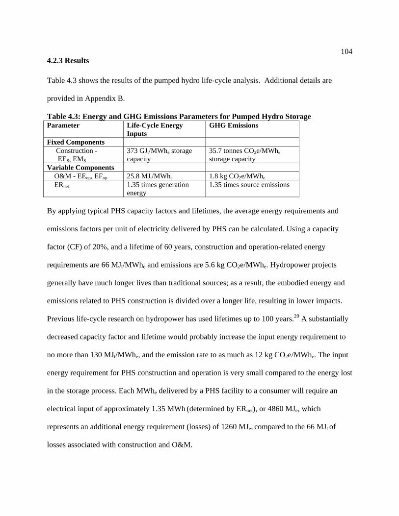
104

4.2.3 Results

Table 4.3 shows the results of the pumped hydro life-cycle analysis. Additional details are

provided in Appendix B.

Table 4.3: Energy and GHG Emissions Parameters for Pumped Hydro Storage Parameter Life-Cycle Energy

Inputs GHG Emissions

Fixed Components Construction - EES, EMS

373 GJt/MWhe storage capacity

35.7 tonnes CO2e/MWhe storage capacity

Variable Components O&M - EEop, EFop 25.8 MJt/MWhe 1.8 kg CO2e/MWhe

ERnet 1.35 times generation energy

1.35 times source emissions

By applying typical PHS capacity factors and lifetimes, the average energy requirements and

emissions factors per unit of electricity delivered by PHS can be calculated. Using a capacity

factor (CF) of 20%, and a lifetime of 60 years, construction and operation-related energy

requirements are 66 MJt/MWhe and emissions are 5.6 kg CO2e/MWhe. Hydropower projects

generally have much longer lives than traditional sources; as a result, the embodied energy and

emissions related to PHS construction is divided over a longer life, resulting in lower impacts.

Previous life-cycle research on hydropower has used lifetimes up to 100 years.20 A substantially

decreased capacity factor and lifetime would probably increase the input energy requirement to

no more than 130 MJt/MWhe, and the emission rate to as much as 12 kg CO2e/MWhe. The input

energy requirement for PHS construction and operation is very small compared to the energy lost

in the storage process. Each MWhe delivered by a PHS facility to a consumer will require an

electrical input of approximately 1.35 MWh (determined by ERnet), or 4860 MJe, which

represents an additional energy requirement (losses) of 1260 MJe, compared to the 66 MJt of

losses associated with construction and O&M.

105

4.3 Net Energy and Emissions – Compressed-Air Energy Storage (CAES) Systems Compressed-air energy storage (CAES) plants in Germany and the U.S. have demonstrated their

technical and economic viability for use as utility-scale energy storage.21 The one existing U.S.

facility is a 110 MW, 26 hour plant completed in 1991 by the Alabama Electric Cooperative

(AEC) facility in McIntosh, Alabama.22 While the low price of peaking fuels (oil and gas)

reduced the economic competitiveness of CAES technology during most of the 1980’s and

1990’s, recent increases in fuel prices have prompted renewed interest in CAES.

In 1999, CAES Development Company (CDC) announced plans to build a 2700 MW facility in

Norton, Ohio using an abandoned limestone mine as the storage vessel.23 Another company,

Ridge Energy Storage, has announced plans to develop CAES using salt domes in the Texas.24

The use of CAES with existing or planned wind farms has also been proposed.25,26

Potential CAES sites have been identified in many areas of the U.S. (including the West and

Midwest) and internationally.27,28 If privately developed and operated CAES is successful, it may

hasten the development of these sites. These plants may demonstrate the first large-scale

profitable alternative to pumped hydro storage and may increase the use of CAES technology

worldwide. A pumped hydro facility utilizing the Norton, Ohio limestone mine for the lower

reservoir was proposed, but later cancelled, perhaps demonstrating favorable economics for

CAES facilities when an underground air-tight cavern is available.29

106

Description of System

CAES systems are based on conventional gas turbine technology. A schematic diagram of a gas

turbine and CAES system is provided in Figure 4.3. In a single-cycle gas turbine air is

compressed and then combined with natural gas in a combustion chamber. Combustion produces

high-pressure gas, which is then expanded through a turbine, which drives both a generator and

the input air compressor. The principle of CAES is the utilization of the elastic potential energy

of compressed air. Energy is stored by compressing air into an airtight underground storage

cavern. To extract the stored energy, compressed air is drawn from the storage vessel, heated,

and then expanded through a high-pressure (HP) turbine, which captures some of the energy in

the compressed air. The air is then mixed with fuel and combusted in a low-pressure (LP) gas

turbine. Both the high- and low-pressure expanders are connected to an electrical generator.

Turbine exhaust heat is then captured in the recuperator to pre-heat cavern air (supplemented by

gas burners.)

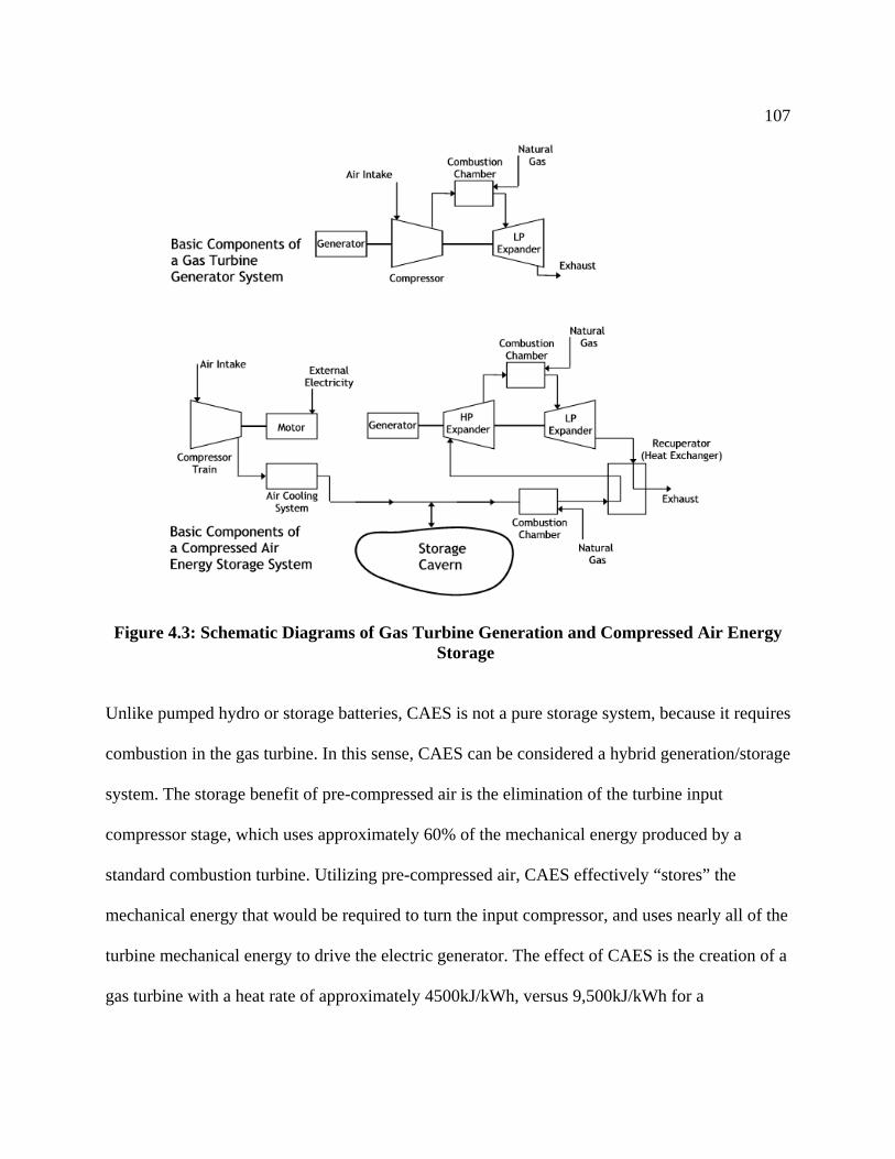
107

Figure 4.3: Schematic Diagrams of Gas Turbine Generation and Compressed Air Energy

Storage

Unlike pumped hydro or storage batteries, CAES is not a pure storage system, because it requires

combustion in the gas turbine. In this sense, CAES can be considered a hybrid generation/storage

system. The storage benefit of pre-compressed air is the elimination of the turbine input

compressor stage, which uses approximately 60% of the mechanical energy produced by a

standard combustion turbine. Utilizing pre-compressed air, CAES effectively “stores” the

mechanical energy that would be required to turn the input compressor, and uses nearly all of the

turbine mechanical energy to drive the electric generator. The effect of CAES is the creation of a

gas turbine with a heat rate of approximately 4500kJ/kWh, versus 9,500kJ/kWh for a

108

conventional single-cycle combustion turbine. Of course, these gains are more than offset by

the energy required to compress the air into the storage vessel.

The AEC’s demonstration system uses a common shaft turbo machinery train, with both

compressors and turbine expanders connected to a common motor-generator set via clutches.30

The next generation of CAES designs use dedicated motor-compressors and generators which

allow for optimally sized and more efficient equipment, as well as faster transition from

compression to generation (or even simultaneous operation) which is important for wind-energy

systems that experience rapid changes in energy output.

While based on gas-turbine technology and requiring natural gas fuel, CAES technology

provides several advantages over gas turbines as a load-following source, enabling intermittent

renewables to be competitive in the peaking power market. These include:

• Very fast ramp rates, greater than traditional peaking gas turbines due to the lack of

input compressor inertia.31 Fast ramp rates allow for load following, as well as

potentially fast response to intermittent renewables.

• Nearly constant heat rate at variable load and ambient conditions due to the constant

fuel/air ratio made possible by a regulated input airflow. CAES also avoids the

decreased efficiencies experienced by gas turbines when compressing hot ambient air

during daytime peaking conditions.

• Low capital costs and system complexities approaching those of single stage CT’s,

due to lack of steam cycle.

109

CAES System Model

The model for the evaluated system is the proposed Norton, Ohio facility, which was approved

by the Ohio Power Siting Board in early 2002. If constructed, this facility would be the largest

CAES system in the world, with peak output of 2700 MW, and a total energy storage capacity of

43.2 GWh (energy/power ratio of 16 hours.)32 The storage cavern is an abandoned limestone

mine with a volume of 9.6 million cubic meters. Since most CAES projects require the

construction of a storage vessel, this study evaluates a salt-solution mined cavern, which is the

likely type of storage vessel for many future CAES projects.33


Site Preparation and Mine Development

Site preparation primarily consists of land clearing and mine development. Salt solution mining

consists of injecting heated water into a salt dome, and pumping out the resulting brine.

Capital Equipment

Capital equipment includes air compressors and associated cooling equipment, combustion

turbine expanders, inlet air heat recuperators, AC electric generators, and transmission

components. Other system components are similar to a natural gas plant of similar size. 34,35

The use of natural gas fuel requires an increase in gas infrastructure, primarily pipeline and

pumping stations. Energy and emissions data for the natural gas delivery systems and gas turbine

components were derived from a previous study of natural gas systems.36

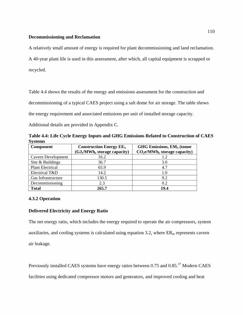
110

Decommissioning and Reclamation

A relatively small amount of energy is required for plant decommissioning and land reclamation.

A 40-year plant life is used in this assessment, after which, all capital equipment is scrapped or

recycled.

Table 4.4 shows the results of the energy and emissions assessment for the construction and

decommissioning of a typical CAES project using a salt dome for air storage. The table shows

the energy requirement and associated emissions per unit of installed storage capacity.

Additional details are provided in Appendix C.

Table 4.4: Life Cycle Energy Inputs and GHG Emissions Related to Construction of CAES Systems Component Construction Energy EES

(GJt/MWhe storage capacity) GHG Emissions, EMS (tonne

CO2e/MWhe storage capacity) Cavern Development 16.2 1.2 Site & Buildings 36.7 3.0 Plant Electrical 65.9 4.7 Electrical T&D 14.2 1.0 Gas Infrastructure 130.5 9.2 Decommissioning 2.3 0.2 Total 265.7 19.4

4.3.2 Operation

Delivered Electricity and Energy Ratio

The net energy ratio, which includes the energy required to operate the air compressors, system

auxiliaries, and cooling systems is calculated using equation 3.2, where ERm represents cavern

air leakage.

Previously installed CAES systems have energy ratios between 0.75 and 0.85.37 Modern CAES

facilities using dedicated compressor motors and generators, and improved cooling and heat

111

recovery systems are expected to have a energy ratio of about 0.7.38 The energy ratio for

CAES systems is less than 1 because additional electricity is generated from natural gas

combustion.

CAES site requirements result in transmission losses similar to those of PHS, and these losses

increase both electricity and natural gas consumption.

Negligible leak rates have been demonstrated in both hard rock mines and salt caverns, resulting

in an ERm ~1. 39,40 No substantially energy-intensive maintenance on either a salt dome or hard

rock cavern is expected over the life of the project. 41,42

Natural Gas Delivery and Combustion

Previous studies of natural gas turbine systems demonstrate a substantial energy requirement for

the exploration, production, and transmission of gas. 43,44 About 1 unit of natural gas is consumed

to deliver 10 units of natural gas to a customer, which results in fairly substantial GHG

emissions.

After heated air is extracted through a high-pressure turbine, it is mixed with natural gas fuel and

combusted in the same manner as a traditional gas turbine. The heat rate (HR) of the combustion

stage is 4536 kJ/kWh.45 The largest component of direct plant emissions results from the

combustion process. Using a standard emission factor of 0.503 g CO2/kJ gas consumed, the

CAES facility produces 228.3 kg CO2e/MWhe from the combustion of natural gas.46

112

Emissions Controls

Selective Catalytic Reduction (SCR) is commonly used in gas turbine power plants to reduce

nitrogen oxide (NOx) emissions.47 SCR utilizes a catalyzed reaction between NOx and ammonia

(NH3), which is injected into the exhaust gas stream. In the presence of a catalyst, NOx, NH3, and

O2 react to form nitrogen gas and water vapor. Energy inputs related to emissions controls are

the production, transportation, and storage of ammonia, as well as the operations of the SCR

equipment.

Life-cycle energy requirements and emissions evaluated by Spath and Mann48 were adjusted to

the CAES heat rate and emission standard49 for this assessment.

Operation and Maintenance

Operation and maintenance includes all daily operations of the plant that have not been

accounted for in construction or fuel usage. This includes repair and replacement of major

mechanical and electrical components, as well as energy associated with cooling water

acquisition and treatment. Energy and emissions data was calculated using EIO data and

estimates for CAES O&M costs.50

4.3.3 Discussion of the Operational and Life-Cycle “Efficiency” of the CAES system

Calculating the overall efficiency of the CAES system is complicated by the use of supplemental

fuel. The simplest method is to calculate the net thermal efficiency of the system:

netthermal ERHR

1 +

=η (4.1)

where HR is the heat rate measured in kWh, reflecting the electrical energy content of the fuel.

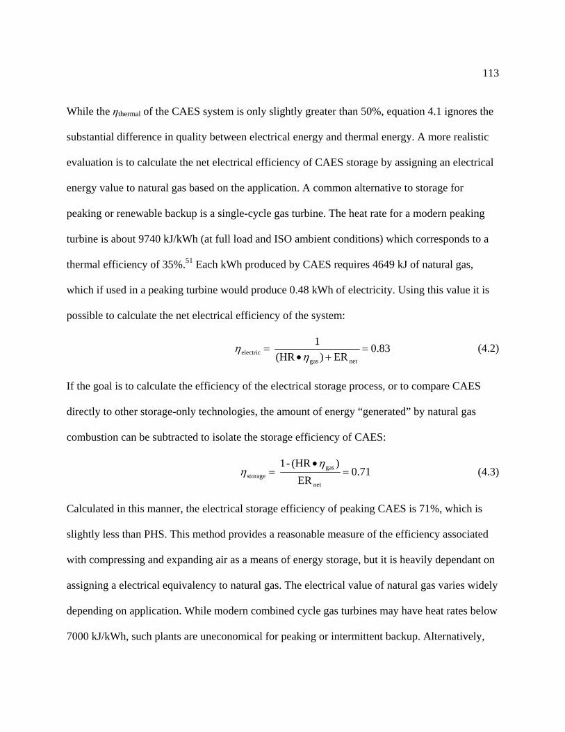
113

While the ηthermal of the CAES system is only slightly greater than 50%, equation 4.1 ignores the

substantial difference in quality between electrical energy and thermal energy. A more realistic

evaluation is to calculate the net electrical efficiency of CAES storage by assigning an electrical

energy value to natural gas based on the application. A common alternative to storage for

peaking or renewable backup is a single-cycle gas turbine. The heat rate for a modern peaking

turbine is about 9740 kJ/kWh (at full load and ISO ambient conditions) which corresponds to a

thermal efficiency of 35%.51 Each kWh produced by CAES requires 4649 kJ of natural gas,

which if used in a peaking turbine would produce 0.48 kWh of electricity. Using this value it is

possible to calculate the net electrical efficiency of the system:

83.0ER)(HR

1 netgas

electric =+•

=η

η (4.2)

If the goal is to calculate the efficiency of the electrical storage process, or to compare CAES

directly to other storage-only technologies, the amount of energy “generated” by natural gas

combustion can be subtracted to isolate the storage efficiency of CAES:

71.0ER

)(HR-1

net

gasstorage =

•=

ηη (4.3)

Calculated in this manner, the electrical storage efficiency of peaking CAES is 71%, which is

slightly less than PHS. This method provides a reasonable measure of the efficiency associated

with compressing and expanding air as a means of energy storage, but it is heavily dependant on

assigning a electrical equivalency to natural gas. The electrical value of natural gas varies widely

depending on application. While modern combined cycle gas turbines may have heat rates below

7000 kJ/kWh, such plants are uneconomical for peaking or intermittent backup. Alternatively,

114

the heat rates of standard peaking gas turbines often exceed 10,000 kJ/kWh when operating

under partial load or high ambient temperatures common in mid-day peaking conditions.

The life cycle efficiency for CAES can be calculated by replacing the ERnet term in equation 4.3

with the denominator term in equation 3.4.

t

LS

Pη

ηη

•⎟⎟⎠

⎞⎜⎜⎝

⎛⎟⎟⎠

⎞⎜⎜⎝

⎛ •++

•−=

Lstor

storopnet

gas

EEEEEER

)(HR1 (4.4)

Figure 4.4 provides a detailed flow of the life-cycle input energy requirements for 1 kWh of

electrical energy delivered by CAES storage, including a 2.5% transmission loss rate on both the

input and output sides of the system.

Figure 4.4: Energy Flow in Compressed Air Energy Storage

115

As can be seen, a majority of the energy requirements are from natural gas. A more detailed

analysis of thermal losses in the CAES process is provided by Zaugg and Stys.52

4.3.4 Results

Table 4.5 shows the results of the CAES life-cycle analysis. Additional details are provided in

Appendix C.

Table 4.5: Energy and Emissions Parameters for Compressed Air Energy Storage

Parameter Life-Cycle Energy Inputs

GHG Emissions

Fixed Components Construction - EES, EMS

266 GJt/MWhe storage capacity

19 tonnes/MWhe storage capacity

Variable Components Fuel 4649 MJt/MWhe 234 kg/MWhe

Fuel Delivery 518 MJt/MWhe 51 kg/MWhe

O&M & SCR 42 MJt/MWhe 3 kg/MWhe

Total Variable - EEop, EFop 5210 MJt/MWhe 288 kg/MWhe

ERnet 0.735 times primary energy

0.735 times source emissions

Average emissions and energy requirements can be estimated using a capacity factor of 20%

and equipment life of 40 years. The generation of 1 MWh of electricity from CAES requires

0.735 MWh of electricity and 5270 MJ of thermal energy, of which only 49 MJ are related to

construction and O&M, with the remainder comprised of natural gas fuel and fuel delivery.

While the energy input requirements of natural gas exceeds the electricity requirements, it is

possible to examine the energy distribution recognizing the greater “value” of electrical energy

compared to thermal energy, as discussed in section 4.3.3. Figure 4.5 shows the distribution of

CAES energy requirements considering the value of 1MJe = 2.5MJt.

116

Normalized Thermal Energy Requirements for CAES Energy

0.4%

4.4%

56.5%

38.7%

Electricity

Gas Fuel

Gas Delivery

Plant, O&M

Figure 4.5: Distribution of CAES Energy Requirements by Source

Excluding primary electricity generation, the total GHG emission rate from CAES is 292 kg

CO2e/MWh. Direct CAES-related emissions mostly result from the combustion and

transportation of natural gas.

4.4 Net Energy and Emissions - Battery Energy Storage (BES)

Utility battery storage is rare due to a variety of factors. Until recently, the only battery

technology that was economically feasible was lead-acid batteries. These batteries are only

marginally economic compared to non-storage alternatives such as diesel generators, and have

substantial space and maintenance requirements. Lead-acid batteries also suffer from a limited

life, which decreases rapidly if the battery is discharged below 30%.53 This effectively reduces

the energy density and increases capital costs. Lead-acid batteries are commonly installed in

uninterruptible power supply (UPS) systems as well as off-grid applications such as renewable

and fossil-based distributed power systems. There are a few utility-scale lead-acid BES systems

in place. Two examples are the 20MW, 14MWh system in Puerto-Rico and the 10MW, 40 MWh

system in Chino, California.54 These systems are designed primarily to solve local power quality

issues as opposed to bulk energy storage as demonstrated by their low energy/power ratio.

117

While lead-acid will likely be the choice for small renewable-storage systems for the near

future, it appears that several new battery technologies are on the verge of surpassing the basic

economic and technical performance of lead-acid batteries for large stationary applications. As a

result, it is likely that future utility scale battery storage will be less likely to utilize lead-acid

technology, but an analysis of lead-acid batteries is important for reference as the “base”

technology.

Perhaps the most promising battery storage technology for large stationary applications to

emerge recently is the flow battery. Flow batteries use liquid electrolytes that are pumped

through a “stack” which contains either an ion-exchange membrane or an electrode array. Three

electrolyte materials have been developed in recent years. These include Vanadium-Acid,

Sodium-Bromide/Sodium-Polysulphide (trademarked as Regenesys) and Zinc-Bromine.55, ,56 57

The Vanadium (typically referred to as Vanadium-Redox Battery or VRB) and Regenesys

(referred to as Polysulfide Battery or PSB) batteries use an ion-exchange membrane similar to

fuel cells, and are sometimes referred to as regenerative fuel cells (RFCs). These two

technologies are the most flexible in size and best suited for very large storage applications, so

they are the representative technologies evaluated in this study. Figure 4.6 shows a schematic of

the basic RFC-type flow-battery components.

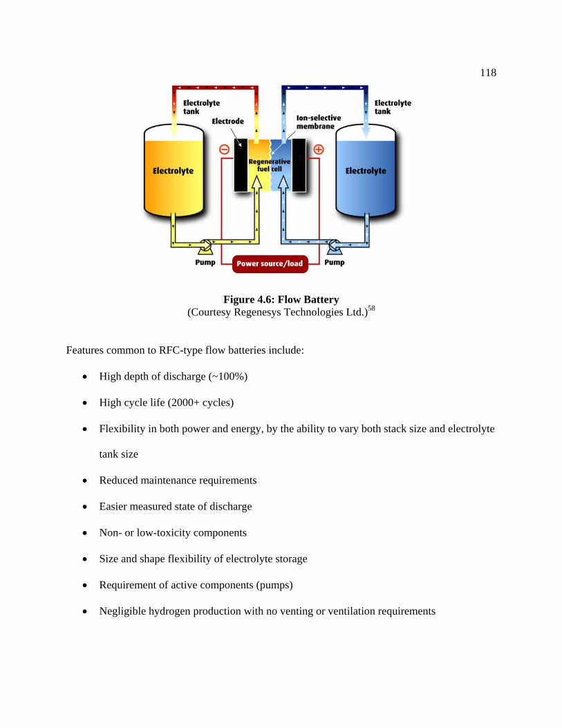
118

Figure 4.6: Flow Battery (Courtesy Regenesys Technologies Ltd.)58

Features common to RFC-type flow batteries include:

• High depth of discharge (~100%)

• High cycle life (2000+ cycles)

• Flexibility in both power and energy, by the ability to vary both stack size and electrolyte

tank size

• Reduced maintenance requirements

• Easier measured state of discharge

• Non- or low-toxicity components

• Size and shape flexibility of electrolyte storage

• Requirement of active components (pumps)

• Negligible hydrogen production with no venting or ventilation requirements

119

Large flow batteries are still in the very early stages of commercialization. A 2 MWh

Vanadium battery was installed near Moab, Utah in 2003. A 15 MW, 120MWh Regenesys

system was planned for installation near Columbus Mississippi, 59 but the Regenesys parent

company discontinued technology development in the end of 2003.60 The technology is still

considered commercially viable and is now being pursued by other parties.61

Functional Unit Definition

This assessment assumes a large BES system with an energy/power ratio of 8 hours, which

approximates the energy/power ratio of PHS and CAES systems. The lead-acid BES system is

based on the Chino installation, while the PSB and VRB systems are based on the proposed TVA

Regenesys project.


Site Preparation and Structures

A BES facility is typically much smaller than a PHS or CAES facility, largely because there are

no geological requirements, fewer economy of scale factors, and because BES facilities can be

placed close to the load. Site buildings are dependent on the type of battery: lead-acid batteries

can be housed in a single enclosed structure, while flow batteries may use separate external

storage tanks, depending on the application. The presence of potentially hazardous liquid

electrolytes may restrict siting and require additional monitoring and containment equipment.62

Figure 4.7 shows the basic features of a large 15 MW, 120 MWh flow battery system, including

external electrolyte tanks, and an enclosed structure that contains the stack and PCS system. For

a 120 MWh PSB, two freestanding electrolyte storage tanks are required, each with a volume of

approximately 2 million liters.63 A VRB system of similar energy capacity would require

120

approximately 6 million liters of electrolyte.64 The flow battery system would occupy

approximately 1.6 hectares of a 5 hectare site.65

Figure 4.7: Artist’s Rendering of a Complete Utility Scale BES system (Courtesy Regenesys Technologies Ltd.)66

Capital Equipment

A complete BES system consists of the battery stacks, electrolyte materials and infrastructure, as

well as the power conditioning system (PCS), which consists of AC-DC and DC-AC converters

and regulators, and associated cooling equipment. The VRB and PSB are assessed equally for all

components except for those related to the electrolytes and battery stack. Electrolytes were

evaluated using PCA methods based on primary materials. Energy requirements related to the

VRB battery stack are based on a previous study.67

For equal comparison, the lead-acid battery is oversized by 30%, due to its limited (70%) depth

of discharge. During the plant lifetime, the lead-acid batteries will require replacement. This

assessment considers the additional lead-acid battery components to be derived from a closed-

loop recycling process.

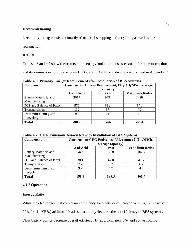
121

Decommissioning

Decommissioning consists primarily of material scrapping and recycling, as well as site

reclamation.

Results

Tables 4.6 and 4.7 show the results of the energy and emissions assessment for the construction

and decommissioning of a complete BES system. Additional details are provided in Appendix D.

Table 4.6: Primary Energy Requirements for Installation of BES Systems Component Construction Energy Requirement, EES (GJt/MWhe storage

capacity) Lead-Acid PSB Vanadium Redox Battery Materials and Manufacturing

2017 943 1439

PCS and Balance of Plant 572 661 671 Transportation 132 87 79 Decommissioning and Recycling

98 64 64

Total 2819 1755 2253

Table 4.7: GHG Emissions Associated with Installation of BES Systems Component Construction GHG Emissions, EMS (tonnes CO2e/MWhe

storage capacity) Lead-Acid PSB Vanadium Redox Battery Materials and Manufacturing

144.9 66.8 102.7

PCS and Balance of Plant 38.1 47.0 47.7 Transportation 7.2 6.7 6.2 Decommissioning and Recycling

9.7 4.7 4.7

Total 199.9 125.3 161.4

4.4.2 Operation Energy Ratio

While the electrochemical conversion efficiency for a battery cell can be very high, (in excess of

90% for the VRB,) additional loads substantially decrease the net efficiency of BES systems.

Flow battery pumps decrease overall efficiency by approximately 3%, and active cooling

122

requirements result in additional losses. Unlike PHS or CAES, batteries store and produce

low voltage direct current, which requires solid-state AC-DC and DC-AC converters; losses

associated with roundtrip AC-AC conversion are at least 4% and can be significantly higher

depending on load conditions.68 Manufacturer’s data and operational experience for the complete

BES system was used to derive an ERnet for each type.69, ,70 71

A substantial advantage of BES is the ability to place the unit at or near the point of use. There

are no geologic requirements, and since there are no operation-related emissions, batteries can be

placed near or in occupied buildings. BES units may be placed at substations for local voltage

support, and may also provide additional economic benefits such as transmission and delivery

(T&D) deferral and increased system reliability. This geographical benefit translates to

substantially reduced transmissions losses associated with BES use as compared with CAES or

PHS. Placement at substations reduces the incremental BES transmission distance to near zero.

Operation and Maintenance Requirements

There are no major consumables associated with BES operation, so additional energy

requirements are derived primarily from system maintenance and repair. Energy and emissions

requirements were calculated using EIO methods based on estimated annual maintenance costs.72

Costs for lead-acid batteries are generally available, while O&M costs for flow-batteries is more

difficult to assess due to a lack of an installed base. Flow batteries are expected to require

substantially less maintenance then lead-acid batteries; primarily electrolyte evaluation, and

periodic replacement of pumps and stack components. Large scale advanced BES systems do not

require full-time manual supervision.

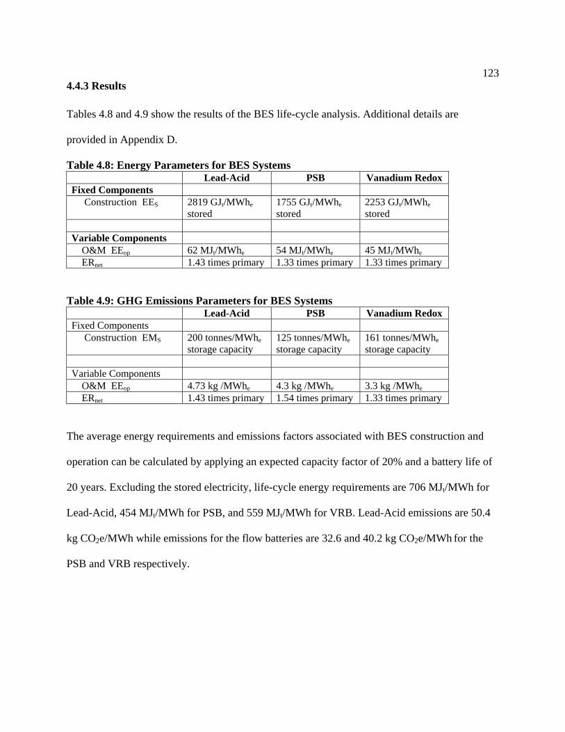
123

4.4.3 Results

Tables 4.8 and 4.9 show the results of the BES life-cycle analysis. Additional details are

provided in Appendix D.

Table 4.8: Energy Parameters for BES Systems Lead-Acid PSB Vanadium Redox Fixed Components Construction EES 2819 GJt/MWhe

stored 1755 GJt/MWhe stored

2253 GJt/MWhe stored

Variable Components O&M EEop 62 MJt/MWhe 54 MJt/MWhe 45 MJt/MWhe

ERnet 1.43 times primary 1.33 times primary 1.33 times primary

Table 4.9: GHG Emissions Parameters for BES Systems Lead-Acid PSB Vanadium Redox Fixed Components Construction EMS 200 tonnes/MWhe

storage capacity 125 tonnes/MWhe storage capacity

161 tonnes/MWhe storage capacity

Variable Components O&M EEop 4.73 kg /MWhe 4.3 kg /MWhe 3.3 kg /MWhe

ERnet 1.43 times primary 1.54 times primary 1.33 times primary

The average energy requirements and emissions factors associated with BES construction and

operation can be calculated by applying an expected capacity factor of 20% and a battery life of

20 years. Excluding the stored electricity, life-cycle energy requirements are 706 MJt/MWh for

Lead-Acid, 454 MJt/MWh for PSB, and 559 MJt/MWh for VRB. Lead-Acid emissions are 50.4

kg CO2e/MWh while emissions for the flow batteries are 32.6 and 40.2 kg CO2e/MWh for the

PSB and VRB respectively.

124

4.5 Comparison of Storage Technologies

4.5.1 Construction Energy

BES systems have substantially greater (roughly 4-8 times) the energy requirements associated

with plant construction compared to equivalent size PHS and CAES systems. Salt solution

mining and earth dam preparation for CAES and PHS are relatively low in energy intensity

compared with building structures to house battery components and electrolytes. The geologic

components of CAES and PHS are also very long-lived compared to batteries. PHS and CAES

use essentially energy-free storage media (water or air) as opposed to BES electrolytes, which

require energy intensive mining and ore processing. Energy requirements for the power

components of battery systems are also much higher than those for PHS and CAES. Turbines,

compressors, and generators are simpler in terms of materials and manufacturing per unit power

compared to battery electrodes, stacks, and PCS equipment. Batteries also require much more

transportation energy, considering the large mass of electrolytes.

O&M energy requirements for BES systems are slightly higher than PHS or CAES systems,

likely due to the comparatively complicated storage medium and power conversion equipment.

4.5.2 Operational Efficiency

The large variability in efficiencies makes a direct comparison between storage technologies

complicated. The VRB has the highest net efficiency of about 75%, with PHS being only 1%

lower. Both the lead-acid and PSB batteries have significantly lower round-trip efficiencies. The

additional inefficiencies in PHS resulting from additional transmission is more than offset by the

DC-AC conversion process, as well as heating, cooling and electrolyte pumping requirements

125

from BES systems. As previously discussed, deriving a true efficiency for CAES requires a

number of assumptions about the electrical “value” of natural gas, but the efficiency of the

electricity storage component can be considered about the same as PHS.

4.5.3 Life-Cycle Energy and Efficiency

The parameters for calculating the life-cycle efficiency for each storage system are reported in

Table 4.10.

Table 4.10: Life-Cycle Energy Parameters for Electricity Storage Systems

Parameter PHS CAES Pb-Acid VRB PSB Estimated Plant Life (years) 60 40 20 20 20 Estimated Capacity Factor (%) 20 20 20 20 20 ERnet 1.35 0.735 1.43 1.33 1.54 Construction and O&M* Energy Ratio (GWhin/GWhout)

0.01 0.07 0.07 0.06 0.04

Fuel Energy Ratio (GWhin/GWhout)

0 0.48 0 0 0

Life-Cycle Efficiency, Lsη 74% 65% 66% 72% 63%

*Includes delivery of natural gas fuel for CAES

With the exception of CAES, the net energy requirements for storage systems are dominated by

the input electricity, most of which is “passed through” the system. Identifying the sources of

energy losses is of potentially greater value. Figure 4.8 shows the distribution of system losses

for each MWh of electricity delivered by the energy storage system.

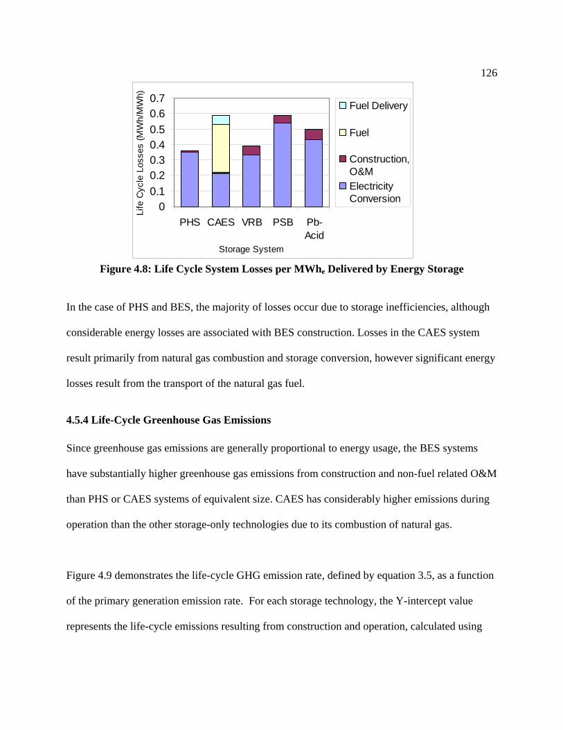
126

00.10.20.30.40.50.60.7

PHS CAES VRB PSB Pb-Acid

Storage System

Life

Cyc

le L

osse

s (M

Wh/

MW

h)

Fuel Delivery

Fuel

Construction,O&MElectricityConversion

Figure 4.8: Life Cycle System Losses per MWhe Delivered by Energy Storage

In the case of PHS and BES, the majority of losses occur due to storage inefficiencies, although

considerable energy losses are associated with BES construction. Losses in the CAES system

result primarily from natural gas combustion and storage conversion, however significant energy

losses result from the transport of the natural gas fuel.

4.5.4 Life-Cycle Greenhouse Gas Emissions

Since greenhouse gas emissions are generally proportional to energy usage, the BES systems

have substantially higher greenhouse gas emissions from construction and non-fuel related O&M

than PHS or CAES systems of equivalent size. CAES has considerably higher emissions during

operation than the other storage-only technologies due to its combustion of natural gas.

Figure 4.9 demonstrates the life-cycle GHG emission rate, defined by equation 3.5, as a function

of the primary generation emission rate. For each storage technology, the Y-intercept value

represents the life-cycle emissions resulting from construction and operation, calculated using

127

the plant lifetimes and capacity factors in reported Table 4.11. The slope represents the net

energy ratio.

0

200

400

600

800

1000

1200

1400

1600

0 100 200 300 400 500 600 700 800 900 1000Electricity Source GHG Emissions (kg CO2e./MWh)

Life

-Cyc

le S

tora

ge G

HG

Em

issi

ons

(kg

CO

2e/M

Wh)

PSB

Pb-Acid

VRB

PHS

CAES

Nuclear /Renewable

Natural Gas CCGT Coal

Figure 4.9: Life Cycle GHG Emissions from Electricity Storage Systems as a Function of

Primary Electricity Source GHG Emissions

The three categories of generation are labeled on the top of the x-axis in Figure 4.9, based on

emission rates provided in Table 3.1. The range of emission rates in Figure 4.9 reflects this large

variation in primary electricity emissions. Due to natural gas combustion, CAES exhibits higher

GHG emissions than PHS or BES when coupled to low GHG electricity generation. As

emissions from the primary electricity generation increase, CAES becomes more favorable. The

emissions rate from CAES equals the rate from non-combustion storage systems when the

electricity source emissions rate is between 325 and 475 kg CO2e/MWh. This value is equal to or

less than the minimum emissions from currently available fossil generation technology. As a

128

result, CAES is the lowest GHG emitting storage technology when coupled with gas, oil, and

coal generation sources.

The unique features of CAES, including a low energy ratio (ERs<1), and the use of natural gas

for the “remainder” of the electricity generated results in a large difference of over 300 kg

CO2e./MWh between it and PHS or BES using current coal-derived electricity. The effect of

“fuel switching” in the CAES system substantially reduces GHG emissions and makes CAES the

preferred technology to store electricity derived from coal.

PHS and the VRB BES are generally similar in performance with regard to GHG emissions, with

PHS having slightly lower overall GHG emissions due to lower construction related emissions.

The low round-trip efficiency of the lead-acid and PSB batteries results in the highest level of

emissions when coupled with fossil sources.

4.5.5 Future Developments

PHS is a very mature technology, with little forecast improvement for either energy input or

efficiency. Improved turbines, along with other improvements in CAES technology are possible,

although these improvements will be incremental in nature.73 A number of improvements in BES

systems could potentially improved their environmental performance. Improved electrolyte

manufacturing techniques could decrease energy intensity, while increased efficiency of PCS

may improve the round trip efficiency. Increased use of recycled materials would also

dramatically reduce energy and emissions from BES systems. The VRB particularly could

benefit from secondary material recovering from industrial processes.74 The most significant

129

improvement would likely result from the development of new electrolyte materials, with

lithium based electrolytes currently being the most promising.75


1 Electricity Storage Association (2002) Via

http://www.electricitystorage.org/technology/ratings.htm. Accessed 8/27/02. 2 Gallob, J. A. (1990). In Search of Beneficial Environmental Impacts: Superconductive

Magnetic Energy Storage, The National Environmental Policy Act and an Analysis of Environmental Benefits. Harvard Environmental Law Review 14: pp. 411-486.

3 Luongo, C. A. (1996). Superconducting storage systems: an overview. IEEE Transactions on

Magnetics 32(4 part 1): pp. 2214-2223. 4 Feak, S. (1997). Superconducting Magnetic Energy Storage (SMES) Utility Application

Studies. IEEE Transactions on Power Systems 12(3): pp. 1094-2003. 5 Sels, T., et al. (2001). New energy storage devices for an improved load managing on

distribution level. 2001 IEEE Porto Power Tech Proceedings. 6 Hockney, R. L. and C. A. Driscoll (1997). Powering of Standby Power Supplies Using

Flywheel Energy Storage. INTELEC 9. 7 Padró, C. E. G. and V. Putsche (1999). Survey of the Economics of Hydrogen Technologies.

National Renewable Energy Laboratory. Golden, Colorado. NREL/TP-570-27079. 8 Ter-Gazarian, A. and Institution of Electrical Engineers. (1994). Energy storage for power

systems. Stevenage, Peter Peregrinus on behalf of the Institution of Electrical Engineers. 9 Task Committee on Pumped Storage of the Hydropower Committee of the Energy Division of

the American Society of Civil Engineers. (1993.) Compendium of Pumped Storage Plants in the United States (American Society of Civil Engineers, New York.

10 Strauss, P. L. (1991). Pumped storage, the environment and mitigation. Waterpower 91, New

York. 11 Tanaka, H. (2000). The role of pumped-storage in the 21st century. International Journal on

Hydropower & Dams 7(1): pp. 27. 12 U.S Department of Energy. (1992). Electric Plant Cost and Power Production Expenses 1990.

Energy Information Agency. DOE/EIA-0455(90). Washington, D.C.

130

13 Gagnon, L. and J. Van de Vate (1997). Greenhouse gas emissions from hydropower. Energy

Policy 25(1): pp. 7-13. 14 Rosa, L. P. and M. A. dos Santos (2000). Certainty & Uncertainty in the Science of

Greenhouse Gas Emissions from Hydroelectric Reservoirs (Part 2) Thematic Review. World Commission on Dams.

15 Ter-Gazarian(1994). 16 Sadden, B. E. (1990). Mainenance of Pumped Storage Plants. Pumped Storage: Proceedings

of the conference organized by the Institution of Civil Engineers at Imperial College of Science, Technology and Medicine, London, The Institution of Civil Engineers.

17 Ramacumar, R., et al. (1993). Economic Aspects of Advanced Energy Technologies.

PROCEEDINGS OF THE IEEE 81(3): pp. 318-332. 18 Schoenung, S. M. and C. Burns (1996). Utility energy storage applications studies. IEEE

Transactions on Energy Conversion 11(3): pp. p. 658-65. 19 Ferreira, A. (1990). Sixteen Years Operating and Maintenance Experience of the 1080 MW

Northfield Mountain Pumped Storage Plant. Pumped Storage: Proceedings of the conference organized by the Institution of Civil Engineers at Imperial College of Science, Technology and Medicine, London, The Institution of Civil Engineers.

20 Gagnon, L. and J. Van de Vate (1997). 21 Ter-Gazarian (1994). 22 Boutacoff, D. (1989). Pioneering CAES for Energy Storage. EPRI Journal: pp. 31-39. 23 Norton Energy Storage L.L.C. (2000). Application to the Ohio Power Siting Board for a

Certificate of Environmental Compatibility and Public Need. Summit County, Ohio. 24 Ridge Energy Corporation. (2002) Via http://www.ridgeenergystorage.com/ Accessed 8/27/02. 25 Desai, N., et al. (2003). Study of Electric Transmission in Conjunction with Energy Storage

Technology. Texas State Energy Conservation Office. 26 Iowa Stored Energy Project. (2004). Via http://www.idea.iastate.edu/isep/index.asp. Accessed

March 4, 2004. 27 Cavallo, A. J. (2001). Energy Storage Technologies for Utility Scale Intermittent Renewable

Energy Systems. Journal of Solar Energy Engineering 123: pp. 387-389.

131

28 Ter-Gazarian (1994). 29 Willett, D. C. (1990). Summit Hydroelectric Pumped Storage Project. Pumped Storage:

Proceedings of the conference organized by the Institution of Civil Engineers at Imperial College of Science, Technology and Medicine, London, The Institution of Civil Engineers.

30 Hounslow, D. R., et al. (1998). The development of a combustion system for a 110 MW CAES

plant. Journal of Engineering for Gas Turbines and Power 120(4): pp. 875-83. 31 Ridge Energy Corporation. (2002) . 32 Norton Energy Storage L.L.C. (2000). 33 Ridge Energy Corporation. (2002). 34 Electric Power Research Institute. (1994). Standard compressed-air energy storage plant:

design and cost. EPRI. Palo Alto, Calif. TR-103209. 35 Shepard, S. and S. v. d. Linden (2001). Compressed air energy storage adapts proven

technology to address market opportunities. Power Engineering 105(4): pp. 34-37. 36 Meier, P. J. and G. L. Kulcinski (2000). Life-Cycle Energy Cost and Greenhouse Gas

Emissions for Gas Turbine Power. Energy Center of Wisconsin. Research Report 202-1. 37 Totten, P. A., et al. (1989). Electricity From Air. Civil Engineering (July). 38 Norton Energy Storage L.L.C. (2000). 39 King, M. J., et al. (2000). Norton Compressed-Air Energy Storage Project: Air Storage System

Characterization and Performance Review. The Hydrodynamics Group. LLC. Edmonds, WA. 40 Ter-Gazarian (1994). 41 Bauer, S. J. and S. W. Webb (2000). Summary Report on Studies and Analyses Supporting

Underground Aspects of a CAES Facility at Norton, Ohio. Sandia National Laboratories. Albuquerque. SAND2000-3111.

42 Crotogino, F. and K. U. Mohmeyer (2001). Huntorf CAES: More than 20 Years of Successful

Operation. Solution Mining Research Institute Spring 2001 Meeting, Orlando, Florida, USA. 43 Meier, P. J. and G. L. Kulcinski (2000). 44 Spath, P. L. and M. K. Mann (2000). Life Cycle Assessment of a Natural Gas Combined-Cycle


132

45 Norton Energy Storage L.L.C. (2000). 46 U.S. Environmental Protection Agency (1996). 5th Edition AP-42. Compilation of Air

Pollutant Emission Factors, AP-42, Fifth Edition, Volume I: Stationary Point and Area Sources.

47 Biewald, B., et al. (2000). Use of Selective Catalytic Reduction for Control of NOx Emissions

from Power Plants in the U.S. Synapse Energy Economics, Inc. 48 Spath, P. L. and M. K. Mann (2000). 49 Norton Energy Storage L.L.C. (2000). 50 Ibid. 51 Siemens AG. (2002) Via http://www.siemenswestinghouse.com/en/ratings/index.cfm.

Accessed 6/10/02. 52 Zaugg, P. and Z. S. Stys (1980). Air-Storage Power Plants with Special Consideration of USA

Conditions. Brown Boveri Review 67: pp. 723-733. 53 Rydh, C. J. (1999). Environmental assessment of vanadium redox and lead-acid batteries for

stationary energy storage. Journal of Power Sources 80: pp. 21-29. 54 Parker, C. D. (2001). Lead-Acid Battery Energy-Storage Systems for Electricity Supply

Networks. Journal of Power Sources 100: pp. 18-24. 55 Price, A., et al. (1999). A novel approach to utility scale energy storage. Power Engineering

Journal 13(3): pp. 122 –129. 56 Lex, P. and B. Jonshagen (1999). The zinc/bromine battery system for utility and remote area

applications. Power Engineering Journal 13(3): pp. 142 -148. 57 Shibata, A. S., K. (1999). Development of vanadium redox flow battery for electricity storage.

Power Engineering Journal 13(3): pp. 130-135. 58 Regenesys Technologies Limited. (2002) Via http://www.regenesys.com/download/index.htm.

Accessed 6/05/02. 59 Tennessee Valley Authority. (2001). Environmental Assessment: The Regenesys Energy

Storage System. Tennessee Valley Authority. Muscle Shoals, Alabama.

133

60 Tennessee Valley Authority. (2001). Current Events. January 9, 2004 Via

http://www.tva.com/finance/info/events_archive/1-9-04.htm Accessed May 1, 2004. 61 Stephen Shaw (2004) Personal Communication. January 17, 2004. 62 Tennessee Valley Authority. (2001). 63 Fairley, P. (2003). Recharging the Power Grid. MIT Technology Review 106(2): pp. 50-57. 64 Shibata, A. S., K. (1999). 65 Tennessee Valley Authority. (2001). 66 Regenesys Technologies Limited. (2002) . 67 Rydh, C. J. (1999). 68 Rodriguez, G. D., et al. (1990). Operating the world's largest lead/acid battery energy storage

system. Journal of Power Sources 31(1-4): pp. 311-320. 69 Lotspeich, C. (2002). A Comparative Assessment of Flow Battery Technologies. Electrical

Energy Storage - Applications and Technology Conference, San Francisco, CA. 70 Price, A. (2000). Technologies for energy storage-Present and future: flow batteries. IEEE

Power Engineering Society Summer Meeting, 2000.vol 3. 71 Tokuda, N., et al. (2002). Development of a redox flow (RF) battery for energy storage.

Proceedings of the 2002 Power Conversion Conference, 2002., Osaka, Japan.vol. 3. 72 Lotspeich, C. (2002). 73 Ter-Gazarian (1994). 74 Hepworth, M. and R. Slimane (1997). Recovery of vanadium, nickel, and carbon from orinoco

crudes via flexicoking. Journal of Solid Waste Technology and Management 24(2): pp. 104-11. 75 Terada, N., et al. (2001). Development of lithium batteries for energy storage and EV

applications. Journal of Power Sources 100(1-2): pp. 80-92.

134

5. Analysis of Electricity Transmission and Distribution Systems An analysis of electricity T&D increases the accuracy of an environmental assessment of

electricity actually used by the consumer. Considering the effects of T&D provides a better basis

to compare the environmental impact of different sources of electricity generation, as T&D

losses vary among these different generation sources. As discussed in section 3, some

intermittent renewable sources have unique T&D requirements that require inclusion of T&D

effects for equal comparison to traditional sources. A life-cycle approach can be used to assess

the effects of T&D losses, as well as effects related to construction and operation of T&D

systems.

5.1 Introduction to Electricity Transmission and Distribution Systems

The T&D system consists of the various components required to deliver electricity from the

generator to the consumer. The number of components required depends on both the type of

generator and the type of customer.

5.1.1 Components of the T&D System

Transmission and distribution consists of several different levels of voltage and current,

depending on proximity to generation or load. Power leaves a generator at high voltage and

current, and voltages are reduced and current paths are split as the power flows towards the

consumer. A general model of a typical T&D system is outlined below and illustrated in Figure

5.1. It consists of the following components:

a) Generation/Step-Up Transformer

135 Nearly all of the electricity used in the U.S. is generated at centralized power stations by

rotating synchronous generators. These generators produce 60 Hz alternating current

(AC) at voltages of 10-20 kV. This voltage is stepped up to the local transmission

voltage, typically between 69-765 kV, depending on the generator’s proximity to a load

center.

b) Extra-High Voltage (EHV) Transmission Line (230, 345, 500 or 765 kV)

Large EHV transmission lines are designed to carry large amounts of power from very

large distant power sources close to load centers. Large power generators, such as

baseload coal and nuclear power plants, are typically located at some distance from

population centers for environmental, safety, or aesthetic reasons. EHV lines typically

carry 500-3000 MW.

c) Splitting/Switching Substation

These stations split the large EHV lines into multiple lines at a lower voltage, so that

several large blocks of power can be brought closer to load centers.

d) High Voltage (HV) Transmission Line (115-230 kV)

HV Transmission lines bring large amounts of power, typically 100-1000 MW, to various

points close to load centers. Intermediate load plants located close to load centers often

tie in at this point.

e) Splitting/Switching Substation

Voltage is again lowered and split into multiple paths to better distribute the power within

a load center. This lower voltage is often referred to as subtransmission.

f) Subtransmission Line (69-130 kV)

136 Subtransmission lines carry smaller blocks of power, typically 50-200 MW through load

centers. Smaller peaking power plants that are located close to or within load centers

often bypass the transmission level and tie in to the subtransmission system.

g) Distribution Substation

A distribution substation converts transmission or subtransmission voltage into

distribution voltage, typically 5-35 kV. Substations are typically located within load

centers, such as residential neighborhoods, or adjacent to end users, such as commercial

or industrial facilities.

h) Distribution/Feeder Line (5-35 kV)

Distribution lines run through residential neighborhoods or commercial areas.

Distribution lines in populated areas typically carry 5-50 MW each.

i) Service Transformer

The service transformer converts distribution voltage to end use voltage, typically

240/120 V for residential users. Service transformers are typically located within 100

meters of the end user. They are either mounted on poles and resemble large cans, or in

areas with underground distribution, are placed in small above-ground structures.

j) Service Line (120/240 V)

These relatively short lines carry end-usable voltage to the consumer’s meter.

The voltage levels for transmission, subtransmission, and distribution are not strictly defined,

and there may be some overlap in definition: 118 kV may be considered transmission in one

system, and subtransmission in another.

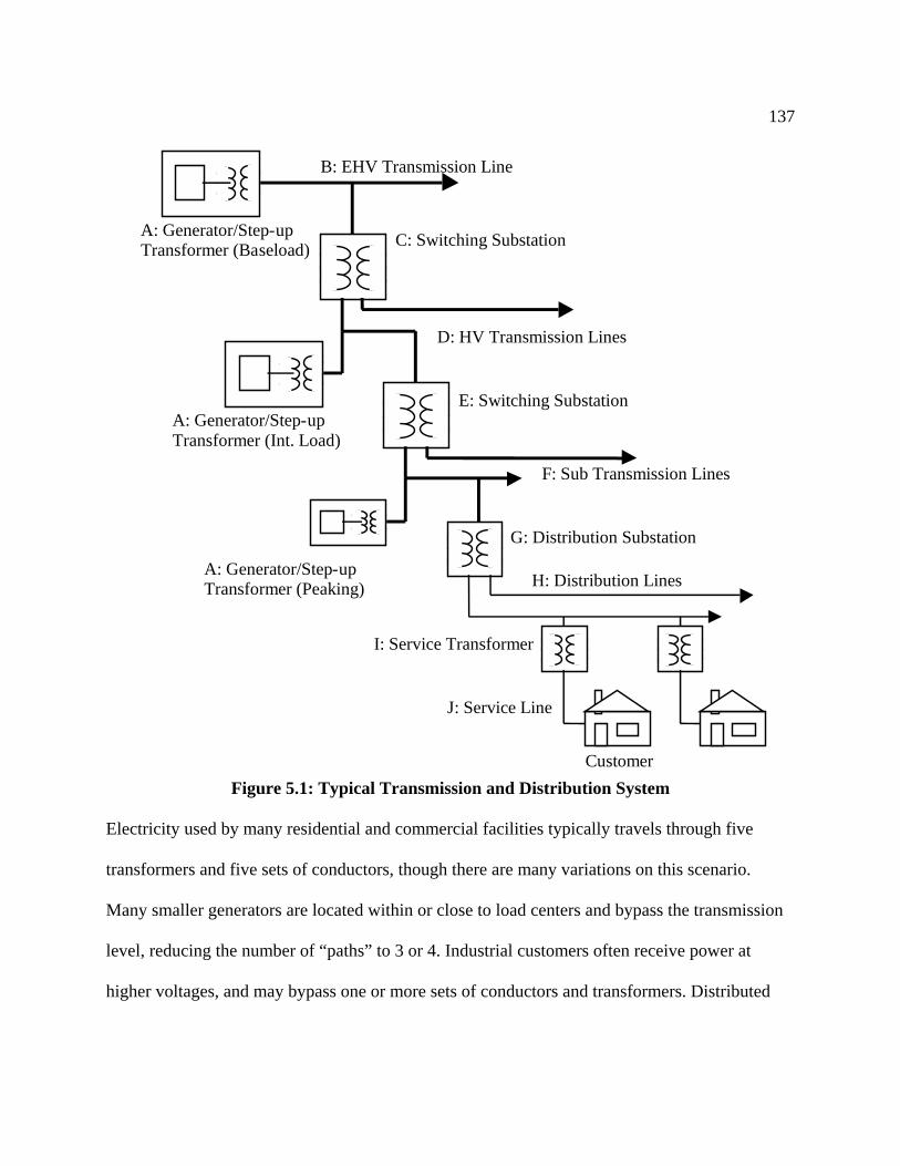
137

B: EHV Transmission Line

C: Switching Substation

D: HV Transmission Lines

F: Sub Transmission Lines

E: Switching Substation

H: Distribution Lines

G: Distribution Substation

A: Generator/Step - up Transformer (Ba seload)

A: Generator/Step - up Transformer (Int. Load)

A: Generator/Step - up Transformer (Peaking)

I: Service Transformer

J: Service Line

Customer

Figure 5.1: Typical Transmission and Distribution System

Electricity used by many residential and commercial facilities typically travels through five

transformers and five sets of conductors, though there are many variations on this scenario.

Many smaller generators are located within or close to load centers and bypass the transmission

level, reducing the number of “paths” to 3 or 4. Industrial customers often receive power at

higher voltages, and may bypass one or more sets of conductors and transformers. Distributed

138 power sources such as solar PV systems may produce electricity at the same location it is used,

and bypass the T&D system altogether.

Additional components in the T&D system are necessary for its safe and efficient operation,

including meters, circuit breakers, switches, fuses, and electronic control systems. In addition,

certain components are required to control the quality of electrical power. The voltage and

current in AC power systems generally do not flow in step with one another. This quality, known

as reactive power, can a have major impact on system operation, stability, and losses, and is

discussed in more detail in section 5.3.

5.1.2 The Existing Transmission System in the U.S.

Bulk transfer of power between regions occurs mostly on EHV lines (230 kV and above.) There

are approximately 254,000 km of EHV lines in the U.S.1 Despite this extensive transmission

network, the majority of electricity used in the U.S. is generated relatively close to its use.

Traditional regulation has required utilities to be relatively self-sufficient in terms of meeting

demand without depending on large amounts of external imports via transmission. In 2002, the

net amount of electricity that flowed across state borders was less than 15%.2

5.2 Alternative Transmission Technologies

While the existing grid is dominated by overhead high voltage AC, there are a number of

alternative technologies that are currently used, or may possibly be used in future transmission

systems.

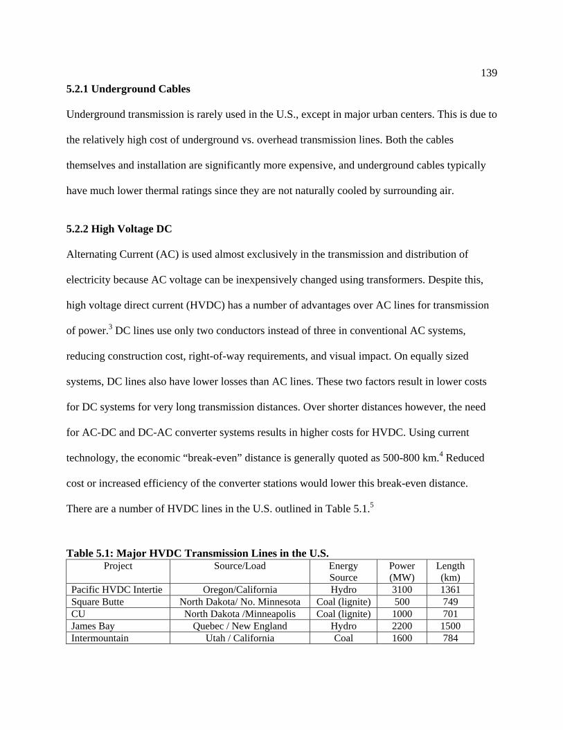
139 5.2.1 Underground Cables

Underground transmission is rarely used in the U.S., except in major urban centers. This is due to

the relatively high cost of underground vs. overhead transmission lines. Both the cables

themselves and installation are significantly more expensive, and underground cables typically

have much lower thermal ratings since they are not naturally cooled by surrounding air.

5.2.2 High Voltage DC

Alternating Current (AC) is used almost exclusively in the transmission and distribution of

electricity because AC voltage can be inexpensively changed using transformers. Despite this,

high voltage direct current (HVDC) has a number of advantages over AC lines for transmission

of power.3 DC lines use only two conductors instead of three in conventional AC systems,

reducing construction cost, right-of-way requirements, and visual impact. On equally sized

systems, DC lines also have lower losses than AC lines. These two factors result in lower costs

for DC systems for very long transmission distances. Over shorter distances however, the need

for AC-DC and DC-AC converter systems results in higher costs for HVDC. Using current

technology, the economic “break-even” distance is generally quoted as 500-800 km.4 Reduced

cost or increased efficiency of the converter stations would lower this break-even distance.

There are a number of HVDC lines in the U.S. outlined in Table 5.1.5

Table 5.1: Major HVDC Transmission Lines in the U.S. Project Source/Load Energy

Source Power (MW)

Length (km)

Pacific HVDC Intertie Oregon/California Hydro 3100 1361 Square Butte North Dakota/ No. Minnesota Coal (lignite) 500 749 CU North Dakota /Minneapolis Coal (lignite) 1000 701 James Bay Quebec / New England Hydro 2200 1500 Intermountain Utah / California Coal 1600 784

140 HVDC technology is a likely candidate for long distance transmission of wind power from the

Midwest to distant load centers.6

5.2.3 Superconducting Transmission Systems

The use of superconducting materials has long been envisioned as an important component of

future transmission systems. Superconductors conduct electricity without losses, and could

greatly increase the amount of power flowing on a single line, reducing the need for large

numbers of conductors to carry power.

Superconducting power cables are still in the development phase, with major use in this decade

unlikely. 7 The largest planned project in the U.S. is a 2000-foot, 600 MW cable scheduled to be

installed on Long Island, NY in 2005.8 Superconducting transmission will not become a

mainstream alternative until there are dramatic reductions in price.

5.2.4 Hydrogen

Hydrogen was not analyzed in this work for either its potential use as an energy storage or

transmission mechanism because of its very high cost, low efficiency, and unlikely near-term

application. The efficiency of long distance transmission of electricity via hydrogen is less than

50%, compared to at least 85% for transmission by wires due largely to the low efficiency of

converting hydrogen into electricity. Even as a combined storage/transmission system it is far

less efficient and cost effective than more conventional alternatives. Its only significant

advantage is the potential ease of siting relative to long distance overhead lines.

141 Hydrogen is not currently competitive as an energy storage or transmission mechanism, but has

been examined as an alternative energy “medium” to integrate renewable energy storage,

transmission, and conversion to transportation fuel. The use of electric/hydrogen systems is often

referred to as the “hydrogen economy” or “hydricity.” The development of such a system will

probably depend on significant reductions (in excess of 90%) in the cost of fuel cells for vehicle

applications.

Hydrogen could eventually be integrated with superconducting transmission technology. The

proposed “continental supergrid” uses underground superconducting transmission cooled by

liquid hydrogen.9 These systems would carry both electricity and hydrogen from remote

generation to major load centers. This very advanced technology will probably not be deployed

before other renewable energy enabling technologies are needed.

5.3 Analysis of Transmission and Distribution Losses

Transmission losses occur in both conductors and transformers. A transmission loss factor for a

delivered unit of energy requires understanding total losses in both the conductor paths and in the

transformers between generator and load.

5.3.1 Conductor Losses

The power losses in a section of conductor are primarily a function of resistance and current,

given by the relationship

P=I2R (5.1)

Resistance is primarily a function of conductor type, size, line length, and temperature. Utilities

choose conductor size and type by balancing the economic benefits of lower losses with the

142 increased cost of more efficient conductors. Utilities also use the maximum possible voltage at

each transmission stage, which keeps line current and system losses to a minimum.

Data on line resistance and voltage is easily obtainable, so an estimate of instantaneous losses

can be calculated using equation 5.1 if line power flow is known. Determining average

transmission line losses is more complex. Power flow through a conductor is seldom constant,

and since transmission losses are proportional to the square of the current transmitted, it is not

possible to simply multiply the total power transmitted by a constant loss factor. There are

additional losses due to secondary effects, discussed in Appendix E.

In addition, reactive power effects can be substantial and must be considered. Reactive power

results from the fact that the current and voltage in a conductor may not be in-phase. The result

of reactive power is increased current flow for a given amount of power, resulting in higher

losses. The amount of reactive power depends on system conditions, which vary over time.

Appendix E provides a sample loss calculation for a proposed Midwestern transmission line, and

describes methods used by utilities to estimate conductor losses for planning purposes.

5.3.2 Transformer Losses

Transformers change voltage from one level to another to facilitate the transmission of

electricity. Transformers pass current through coils of wire which creates a varying magnetic

field which then passes through another coil of wire, inducing a current at higher or lower

143 voltage. The voltage change is determined by the ratio of coils on the primary and secondary

side. Losses in transformers are categorized as two types: load losses and no-load losses.10

Load losses are primarily a result of resistance in the transformer windings, and the losses vary

with the amount of power being transmitted as described by equation 5.1. No-load losses result

from magnetic inefficiencies in the transformer, and are independent of power consumption,

similar in nature to “phantom loads” in appliances, which occur even when the device is turned

off.

Due to the variation of load-losses, and other factors, average transformer efficiencies are easiest

to determine by direct measurement. Typically, efficiencies for large transmission-level

transformers are extremely high. Efficiencies for large utility transformers used at generators and

substations are often above 99.8%. The total combined efficiency for the transformer sections

associated with power transmission (items A,C, and E in Figure 5.1) can often exceed 99%.

Efficiencies for smaller distribution transformers and service transformers are much lower.

Transformers are most efficient when operated at full load, and distribution and service

transformers are typically used at much less than full load. Efficiencies of small distribution

transformers are typically in the 98%-99% range, while service transformers are typically 96%-

99% efficient. The high level of losses in service transformers puts an upper bound on the overall

efficiency of the T&D system. At least 1% (and probably closer to 2%) of the electricity

generated and delivered to low-voltage consumers in the U.S. is lost in the final transformer

stage.

144 5.3.3 Transmission Loss Evaluation for Conventional Generation

In theory, deriving loss factors for a complete electric power system is possible, but would

require a vast amount of data about the system. Data required would include:

• Composition and length of each transmission and distribution line.

• Total load on each transmission line at each moment, including power factor (a measure

of reactive power.)

• Loss rate on each transformer.

• Total load on each transformer at each moment, including power factor.

Knowing the path of electricity flow is extremely difficult. Electricity may travel through many

different paths at different times, so modeling the system requires knowledge of conditions

throughout a region. Utilities and system operators use very powerful (and expensive)

simulations to estimate losses for load forecasting and economic planning, and use vast amounts

of often proprietary data to model regional T&D systems. Not only is certain data proprietary,

previously available data is now restricted. FERC Form 715, which provides substantial details

about transmission system loads, has been removed from the public domain since the Sept 11,

2001 terrorist attacks. In addition, many utilities, state agencies and system operators have also

restricted public access to information about transmission systems. Without complete system

data, estimating transmission losses from this “bottom-up” approach is unrealistic in anything

but the simplest cases.

145 As an alternative to such calculations, publicly available loss data recorded by utilities and other

electricity service providers can be used to reasonably estimate losses in T&D systems. Data

from different electricity providers can be used to determine loss rates for various sections of the

system, including local distribution, T&D within a region, or transmission of electricity between

regions. Such methods are limited by the amount of data available, but can provide a reasonable

estimate of T&D losses at the system level.

In general, transmission losses are a function of proximity of generator to load centers. Loss rates

were evaluated for two general classes of generators: transmission level sources and

subtransmission level sources.

Transmission level sources are plants generally located outside a load center, and feed into the

EHV system. These are typically baseload sources such as coal and nuclear plants.

Subtransmission level sources are generally smaller power plants that provide intermediate load,

or peaking service. A large fraction of these plants are natural gas and oil-fired turbines and

reciprocating generators, although some smaller coal-fired plants operate partially as

intermediate load and peaking facilities.

5.3.4 Transmission Loss Evaluation for Long Distance Transmission

Long distance transmission is used for a relatively small amount of the electricity used in the

U.S. There are two general categories of long distance transmission. The first is transmission that

occurs on multiple paths on the conventional EHV system. An example would be the flow of

146 electricity from an existing generator in Minnesota to Chicago, where the electricity would flow

along multiple lines, and be difficult to precisely identify. Average loss rates for long distance

transmission must be quantified to facilitate deregulated market transactions. As a result,

regional transmission organizations, such as the Midwest Independent System Operator, have

developed estimates of average loss rates that occur between various systems, which can be

applied to estimate losses between a specific generator and load area.

The second class of long distance transmission is the flow of electricity on a limited number of

dedicated point to point lines, such as the two coal by wire HVDC lines running from North

Dakota to eastern Minnesota. Loss rates for point-to-point transmission can be directly based on

I2R losses if the voltage, conductor properties, and load characteristics are known.

5.3.5 Distribution Loss Evaluation

While transmission losses are generally a function of distance, distribution losses are a function

of both distance and customer type. Customer type may be categorized by the size and type of

load. Distribution is a major component of power delivery to most residential and commercial

customers, while industrial customers may bypass distribution completely.

Distribution losses were evaluated by examining loss rate records for utility systems that include

only distribution. These systems include municipals, co-ops, and small local utilities, which

meter their incoming electricity at a distribution substation. A total of 107 systems were

examined. Utility and industry data can also be used to identify loss rate differences between

customer classes.

147 5.3.6 Results

It is impossible to precisely determine the T&D losses for any particular class of generation

technology or customer. However, analysis can provide a typical loss rate, as well as a typical

loss range for a representative group. Given this limitation, Table 5.2 and 5.3 provides estimates

for total transmission and distribution losses based on generator and customer class for utilities in

the upper Midwestern U.S. The first data column in each table provides a typical or

representative loss rate for each class. The second column provides the typical range of results

Table 5.2: Typical Transmission Loss Rates for Electricity Generated in the Upper Midwestern U.S.

Type Typical Loss Rate (%)

Typical Loss Range (%)

Subtransmission-level Sources 0.5% 0.5-2% Transmission-Level Sources (Urban) 1.8% 1-2% Transmission-Level Sources (Rural) 3.6% 2-6% Long Distance on EHV system 3.7% 2-10% Long Distance on HVDC system 6.4% 5-9%

Table 5.3: Typical Distribution Loss Rates for Electricity Consumed in the Upper Midwestern U.S.

Type Typical Loss Rate (%)

Typical Loss Range (%)

Urban Customers (Average of all types) 3.6% 2-8% Urban Customer (Residential/Commercial) 4.1% 3-10% Rural Customer (Average of all types) 6.3% 5-10% Rural Customer (Residential/Commercial) 6.9% 5-12%

From Tables 5.2 and 5.3, a total T&D loss rate can be determined by summing the loss rates for

the appropriate generator type and consumer. As an example, a typical urban residential

customer receiving power from a baseload coal plant would incur a total T&D loss rate of about

5.9% (1.8% + 4.1%), while a typical loss rate for a rural residence would be about 10.5% (3.6%

+ 6.9%).

148

5.4 Analysis of T&D Operation and Maintenance

Operation and maintenance (O&M) of T&D systems results in emissions from two major

sources. Fossil fuel combustion is associated with the periodic maintenance and replacement of

T&D components such as lines, cables, poles and service transformers. In addition, certain

transmission equipment releases sulfur hexafluoride, a potent greenhouse gas.

5.4.1 Energy Requirements and Emissions from System Maintenance

Emissions resulting from system maintenance can be estimated by applying economic

input/output (EIO) emissions factors to annual maintenances costs reported by utilities.

Expenditures for T&D related maintenance were compiled from 6 major utility systems, and 60

municipal electric systems in the upper Midwest for the years 2001 and 2002. EIO data was

applied to this data to derive an effective emissions rate (kg CO2e/MWh transmitted.)

Table 5.4 provides the results of the analysis, and includes a net T&D emissions rate for three

customer types: urban/suburban, rural, and a weighted average of all types.

Table 5.4: GHG Emissions Rates for T&D System Maintenance in the Midwestern U.S.

Utility T&D O&M Cost ($/MWh)

Energy Requirement (GJt./MWh)

GHG Emission Rate (kg CO2e/MWh)

Urban/Suburban Utilities 3.12 1.5 1.5 Rural Utilities 7.03 3.5 3.5 Weighted Average 3.45 1.7 1.7

5.4.2 Sulfur Hexafluoride Emissions

Sulfur Hexafluoride (SF6) is widely used as an insulating gas in large high-voltage circuit

breakers and switchgear.11 It has a number of useful properties, including chemical and thermal

149 stability, and is non-flammable and non-toxic. Its primary disadvantage is its very high global

warming potential, approximately 23,900 times that of CO2 per unit mass. The SF6 emissions

associated with electricity T&D are primarily from leaks in older circuit breakers.

The U.S. EPA SF6 Emissions Reduction Partnership program, tracks emissions of SF6 from 65

electric utilities.12 While emissions of SF6 are not tracked by all utilities, emissions are generally

proportional to transmission system size; estimates from reporting utilities can be applied to

other utilities if transmission size is known. Total average SF6 emissions were estimated based on

various reporting utilities. 13,14

Based on this data, GHG emissions associated with SF6 emissions are roughly 1 kg CO2e/MWh.

A downward trend in SF6 emissions has been reported by most utilities, due largely to

replacement of older equipment and better handling practices, motivated by increasing costs of

SF6 supplies. Since most of the older leaking equipment has been upgraded, the EPA expects this

downward trend to slow and future emission rates to remain roughly constant.

5.5 Construction Related Emissions

As with O&M, the emissions and energy consumption associated with T&D system construction

produces “adders” that may be incorporated with other life-cycle aspects of electricity

generation. This section provides the results of life-cycle analysis that estimates energy

consumption and emissions related to construction of T&D components including transmission

lines, and substations. Net GHG emissions that result from biomass losses in transmission line

right-of-ways are also estimated. The results of this analysis may be used in several ways. Using

150 data from individual components, a complete system may be “assembled” to determine the total

GHG emission rate for a typical T&D system. This can be used to compare conventional

generation to generation technologies that do not require T&D, such as off-grid renewable

energy systems.

Another application of this analysis is to determine the additional energy and GHG burden that

may result from the long distance transmission of distant energy sources such as wind, compared

to conventional generation systems.

5.5.1 Analysis of T&D Lines

Overhead transmission systems consist primarily of conductors and support structures. Most

conductors use aluminum reinforced with steel, referred to as “aluminum conductor, steel-

reinforced” (ACSR). Transmission towers that support EHV lines above 345 kV are most

commonly lattice-type structures constructed of steel and aluminum. A variety of structures are

used to support lines at or below 345 kV and are made of materials such as wood, cement, and

steel. There are many combinations of tower and conductor types. In this study, a representative

sampling of tower and conductor types were chosen for each transmission voltage class and

power level, with a total of 6 different overhead T&D line types.

Analysis primarily used PCA, based on material composition and mass, with EIO methods

applied to construction and installation. Details of the analysis are provided in Appendix F.

151 5.5.2 Effects of Biomass Clearing

Development of transmission line corridors decreases the amount of vegetation present, and can

produce a net increase in atmospheric carbon. To estimate the maximum increase in atmospheric

carbon that results from T&D line installation, it was assumed that trees are cleared, but short

grasses, brush and other vegetation remain. An average Midwestern forest, consisting of Pine,

Spruce, Fir and Oak is estimated to contain 50-80 metric tons of carbon per hectare. This results

in a CO2 emissions factor of 18-29 kg/m2 of forest cleared, if the forest is not allowed to

regenerate.15 Utility data for right-of-way (ROW) requirements were used to estimate total area

required for typical transmission lines. Tree clearing for power line ROW can result in

significant net GHG emissions. A new line that requires complete removal of trees can produce

emission levels greatly exceeding those from line construction. As a result, GHG emissions from

land use may be the most significant aspect of transmission line construction. However, the

actual amount of emissions resulting from ROW development is generally much lower than the

maximum value, since lines may follow roads, previously cleared land, or land with low density

of trees. The majority of line distance in a T&D system is distribution, and most distribution

lines follow roads and other cleared paths that would be developed regardless of the need for

electrical transmission.

While underground lines are generally considered more environmentally friendly due to their

reduced land use and visual impact, emissions from installation of underground lines may exceed

those from overhead conductors, depending on the amount of biomass cleared for each type.

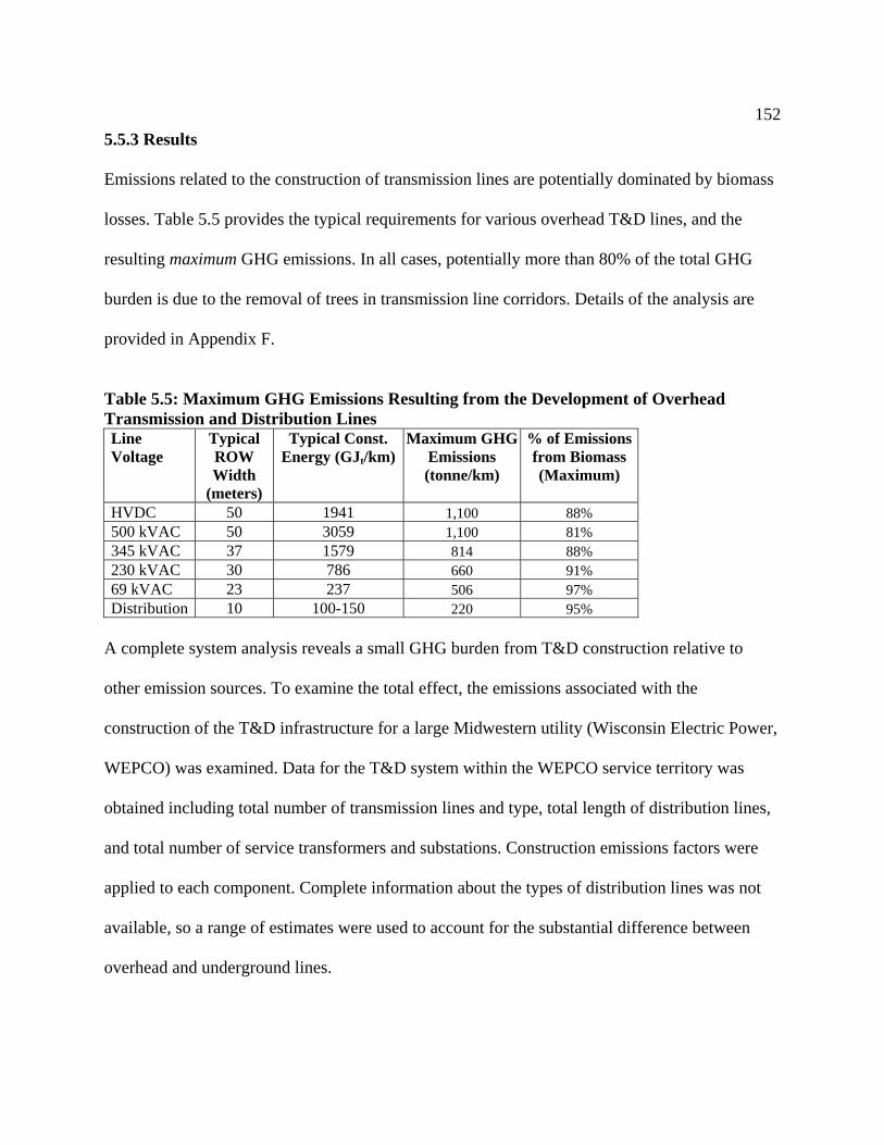
152 5.5.3 Results

Emissions related to the construction of transmission lines are potentially dominated by biomass

losses. Table 5.5 provides the typical requirements for various overhead T&D lines, and the

resulting maximum GHG emissions. In all cases, potentially more than 80% of the total GHG

burden is due to the removal of trees in transmission line corridors. Details of the analysis are

provided in Appendix F.

Table 5.5: Maximum GHG Emissions Resulting from the Development of Overhead Transmission and Distribution Lines Line Voltage

Typical ROW Width

(meters)

Typical Const. Energy (GJt/km)

Maximum GHG Emissions (tonne/km)

% of Emissions from Biomass (Maximum)

HVDC 50 1941 1,100 88% 500 kVAC 50 3059 1,100 81% 345 kVAC 37 1579 814 88% 230 kVAC 30 786 660 91% 69 kVAC 23 237 506 97% Distribution 10 100-150 220 95%

A complete system analysis reveals a small GHG burden from T&D construction relative to

other emission sources. To examine the total effect, the emissions associated with the

construction of the T&D infrastructure for a large Midwestern utility (Wisconsin Electric Power,

WEPCO) was examined. Data for the T&D system within the WEPCO service territory was

obtained including total number of transmission lines and type, total length of distribution lines,

and total number of service transformers and substations. Construction emissions factors were

applied to each component. Complete information about the types of distribution lines was not

available, so a range of estimates were used to account for the substantial difference between

overhead and underground lines.

153 Three estimates were used to derive the emissions factors for T&D construction based on the

system lifetime and amount of land consumed in transmission corridors. The worst case estimate,

using a 20-year lifetime for all components and maximum land use for ROW found an emissions

rate related to T&D construction of about 11 kg CO2e/MWh. A more likely scenario found a rate

of about 5 kg CO2e/MWh, while a best case estimate produced a rate of about 2 kg CO2e/MWh.

While this range of results is large in percentage terms, the absolute burden from construction is

quite small, especially compared to fossil generation and T&D losses.

5.6 Net T&D Effects for Conventional and Renewable Energy Systems

Using the results from sections 5.3 through 5.5, it is possible to estimate the impacts of T&D

losses for different conventional and renewable energy systems.

Table 5.6 shows the life-cycle emissions associated with electricity used by a typical suburban or

urban customer in the Midwestern U.S., including T&D effects, based on average losses

associated with each generator class.

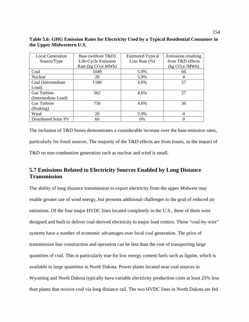
154 Table 5.6: GHG Emission Rates for Electricity Used by a Typical Residential Consumer in the Upper Midwestern U.S.

Local Generation Source/Type

Base (without T&D) Life-Cycle Emission Rate (kg CO2e.MWh)

Estimated Typical Loss Rate (%)

Emissions resulting from T&D effects (kg CO2e./MWh)

Coal 1049 5.9% 66 Nuclear 20 5.9% 4 Coal (Intermediate Load)

1180 4.6% 57

Gas Turbine (Intermediate Load)

562 4.6% 27

Gas Turbine (Peaking)

750 4.6% 36

Wind 20 5.9% 4 Distributed Solar PV 60 0% 0

The inclusion of T&D losses demonstrates a considerable increase over the base emission rates,

particularly for fossil sources. The majority of the T&D effects are from losses, so the impact of

T&D on non-combustion generation such as nuclear and wind is small.

5.7 Emissions Related to Electricity Sources Enabled by Long Distance Transmission

The ability of long distance transmission to export electricity from the upper Midwest may

enable greater use of wind energy, but presents additional challenges to the goal of reduced air

emissions. Of the four major HVDC lines located completely in the U.S., three of them were

designed and built to deliver coal-derived electricity to major load centers. These “coal-by-wire”

systems have a number of economic advantages over local coal generation. The price of

transmission line construction and operation can be less than the cost of transporting large

quantities of coal. This is particularly true for low energy content fuels such as lignite, which is

available in large quantities in North Dakota. Power plants located near coal sources in

Wyoming and North Dakota typically have variable electricity production costs at least 25% less

than plants that receive coal via long distance rail. The two HVDC lines in North Dakota are fed

155 by “mine mouth” generation facilities that have conveyor systems to carry coal directly from the

mine to the power plant.

The most significant, largely exploitable wind energy resources in the U.S. include the low

population areas of western North Dakota and eastern Wyoming. These areas also include much

of the nation’s least expensive coal resources, including the Powder River Basin in Wyoming,

and the rich lignite beds in North Dakota. The coincidence of these two resources presents a

major challenge to the use of wind energy, both from a policy and economic standpoint. Current

policy requires open access of transmission systems, which means that any transmission line

built may not be restricted to any particular utility or fuel source.

There are several proposals to construct major coal by wire systems from Wyoming and North

Dakota. These systems would employ HVDC technology to deliver electricity to major load

centers in California and the Midwest. Some of these proposals include some wind energy, but

only a relatively small fraction, compared to coal based generation. Without storage, wind is

economically limited in terms of the fraction of energy it could produce in a combined coal/wind

energy system, similar to the limits evaluated in Chapter 2.

The export of lignite-derived electricity is of particular interest for a number of reasons. Lignite

is relatively cheap to extract through modern surface mining techniques, but is expensive to

transport, due to its low energy density (energy/mass). This means that unlike Wyoming coal,

lignite is particularly dependent on nearby transmission. The low energy content of the fuel also

produces a higher GHG emission rate relative to other types of coal. Energy providers in North

156 Dakota have proposed the “Lignite 21” project which includes up to 2,000 MW of new

transmission export capacity to be coupled to a new generation of lignite generation facilities.16

The more ambitious TransAmerica Generation Grid (TAGG) proposes 18,000 MW of HVDC

transmission coupled to 4,000 MW of wind, and 14,000 MW of coal, much of which is lignite.17

Table 5.7 reviews the properties of a new 1000 km, 1000MW HVDC power line. This type of

line could provide electricity from lignite or wind energy from North Dakota to a major load

center such as Milwaukee or Chicago. System parameters were based on similar long distance

lines described in Table 5.1.

Table 5.7: Characteristics of a Hypothetical HVDC Line from North Dakota to Eastern Wisconsin or Northern Illinois Voltage +/- 450 kV DC Power 1000 MW Length 1000 km Approximate Cost $650 Million Line + DC Converter Loss Rate 6.4% Total Loss Rate (all T&D) 10.0% Total Annual Losses (based on 85% system capacity factor)

745 GWh

Figure 5.2 illustrates the GHG emissions that would result from electricity delivered by a new

HVDC line powered by a combination of lignite and wind.

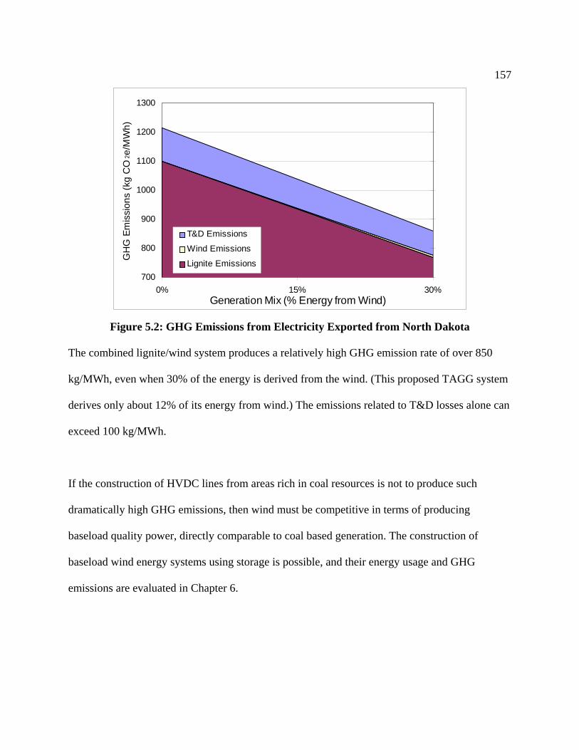
157

700

800

900

1000

1100

1200

1300

0% 15% 30%Generation Mix (% Energy from Wind)

GH

G E

mis

sion

s (k

g C

O 2 e

/MW

h) a

T&D Emissions

Wind Emissions

Lignite Emissions

Figure 5.2: GHG Emissions from Electricity Exported from North Dakota

The combined lignite/wind system produces a relatively high GHG emission rate of over 850

kg/MWh, even when 30% of the energy is derived from the wind. (This proposed TAGG system

derives only about 12% of its energy from wind.) The emissions related to T&D losses alone can

exceed 100 kg/MWh.

If the construction of HVDC lines from areas rich in coal resources is not to produce such

dramatically high GHG emissions, then wind must be competitive in terms of producing

baseload quality power, directly comparable to coal based generation. The construction of

baseload wind energy systems using storage is possible, and their energy usage and GHG

emissions are evaluated in Chapter 6.

158


1 National Electric Reliability Council (2004) Via http://www.nerc.com/~esd/. 2 U.S. Department of Energy. Annual Energy Review 2002. Energy Information Administration:

Washington, DC, 2003. 3 Hauth, R. L., et al. (1997). HVDC Power Transmission Technology Assessment Report. Oak

Ridge National Laboratory . ORNL/Sub/95-SR893/1. 4 Public Service Commission of Wisconsin. (2000). Final Environmental Impact Statement

Arrowhead – Weston Electric Transmission Line Project – Volume 1. Docket 05-CE-113. (2000).

5 CIGRE (1996). Compendium of HVDC Schemes Throughout the World. Version C.

CE/SC:14. 6 Cavallo, A. J. (1995). High-Capacity Factor Wind Energy Systems. Journal of Solar Energy

Engineering 117: pp. 137-143. 7 Politano, D. S., M.; Schnyder, G.; Rhyner, J. (2001). Technical and economical assessment of

HTS cables. IEEE Transactions on Applied Superconductivity 11(1 Part: 2): pp. 2477 -2480. 8 American Superconductor (2003). Via http://www.amsuper.com/ August 20, 2003. 9 Grant, P. (2002). Energy for the City of the Future. The Industrial Physicist 8(1): pp. 22-25. 10 Suechoey, B., et al. (2000). An analysis and selection of distribution transformer for losses

reduction. IEEE Power Engineering Society Winter Meeting, 2000. 11 Christophorou, L. G., et al. (1997). Sulfur hexafluoride and the electric power industry. IEEE

Electrical Insulation Magazine 13(5): pp. 20-24. 12 U.S. Environmental Protection Agency. (2001) SF6 Emissions Reduction Partnership for

Electric Power Systems Annual Report — 2000. 13 Danihel, D. (2003). Senior Environmental Specialist, WE Energies. Personal Communication -

August 12, 2003. 14 Wisconsin Energy Corporation. (2002) Wisconsin Energy Corporation 2001 Performance

Report. 15 U.S. Environmental Protection Agency.(2001) Inventory of U.S. Greenhouse Gas Emissions

and Sinks: 1990-2000.

159 16 Lignite Vision 21 Program. (2004) Via http://www.lignitevision21.com/061402news.htm

Accessed March 3, 2003. 17 Black & Veatch TransAmerica Generation Grid (2004) Via

http://www2.bv.com/services/projects/pd/tagg/technical_sites.asp Accessed March 3, 2004.

160

6. Environmental Assessment of Integrated Renewable/Storage Systems There are a number of likely combinations of intermittent renewable generation and energy

storage, based on utility application and economics. Among the likely possible scenarios are

wind/CAES, wind/PHS, and solar PV/BES.

Wind/CAES is the most likely possibility for near-term renewable storage systems in the U.S.

The vast majority of the wind resources in the U.S. are located in the Midwest, which does not

have the geologic features required for PHS, but does have many locations suitable for CAES.1

There are currently two proposals for the development of CAES for wind energy storage in

Iowa2 and Texas.3

While wind/PHS is unlikely in the Midwestern U.S., there are sufficient wind resources and

geologic features in the far western states for some wind/PHS development. The use of BES for

wind storage is unlikely in the near future due to the high cost. The combination of solar PV and

BES is possible for distributed and peaking power applications, although currently more

expensive than many alternatives.

For these reasons, this analysis of renewable/storage systems focused primarily on wind/CAES,

but provides an analysis of wind/PHS and PV/BES systems for comparison. The life-cycle

energy efficiency and greenhouse gas emissions were evaluated for each of these three

combinations of renewable generation and energy storage.

161

6.1 Environmental Analysis of a Wind/CAES System

Electric power systems in the midwestern U.S. are dominated by coal and nuclear systems. As

previously discussed, these energy sources limit the operational flexibility of utilities and reduce

the opportunity for intermittent wind energy to supply a large fraction of these region’s energy

supply. Wind energy generation, integrated with energy storage, can provide a source of power

functionally equivalent to a baseload coal or nuclear plant, and may be considered as an

alternative to these conventional sources. Baseload wind/CAES systems have been previously

proposed, but not deployed due to the high cost of wind generation. The declining cost of

electricity from wind turbines has now made such systems economically feasible,4 and as a

result, wind/CAES systems may become a significant part of future electric power systems in the

midwestern U.S.

To evaluate the environmental performance of a baseload wind/CAES system, a simulation

model was developed. (The combined wind/CAES system is referred to as a “baseload wind”

system in the remainder of this section.)

The model develops a system that increases the capacity factor of a typical wind generator (25-

40%) to a baseload level (greater than 70%),5 and increases output stability, and predictability.

The development of the model was strongly influenced by the constraints of electricity

transmission. A high system capacity factor is required to maximize the use of expensive

transmission assets. However, the transmission system also establishes the maximum output of

the wind system. As a result, the model is designed to produce an amount of power that is equal

162

to, but does not exceed a level established by the transmission capacity. The effects of losses in

the transmission system were also considered in the model.

6.1.1 System Model

The Wind Energy Storage (WES) model uses a spreadsheet format (Microsoft Excel™) and

simulates the hourly performance of a wind farm integrated with energy storage. Based on wind

energy data and input parameters including storage efficiency and capacity, the WES model

calculates the number of wind turbines and other infrastructure required to deliver performance

similar to traditional baseload sources. The model compares the wind farm output to the target

output on an hourly basis and attempts to provide constant power output by storing, or releasing

from storage, the appropriate amount of energy. The objective of the WES model is to maximize

the use of limited, capital-intensive transmission capacity to provide a constant amount of power

equal to the size of the transmission system. Appendix G provides a logic diagram of the model,

with sample input and output.

The performance of a wind energy system is dependent on a number of factors, including wind

resource, turbine technology, and the size of the wind array. To consider these factors, a total of

seven different cases were evaluated. Each case used at least one full year’s worth of hourly

wind data to consider seasonal variations in wind speed.

Two cases were created to evaluate the performance of modern, state-of-the-art baseload wind

power plants. Case 1 simulates a medium size (in terms of traditional thermal generation)

baseload power plant, with an output of 300 MW, located relatively close to a population center

163

in the Midwestern U.S. Case 2 simulates a large baseload plant, with an output of 1000 MW,

which could serve a significant fraction of the baseload energy demand of a large load center.

The wind farm in Case 2 is located in a very remote, rural location, with excellent wind

resources. Additional details about the two cases are provided in table 6.1.

Table 6.1: System Parameters for Simulated Wind Systems System Parameter Case 1

Case 2

System Size (Constant Power Output – MW)

300 MW 1000 MW

Hub Height (m) 80 100 Avg. wind speed at hub height (m/s)

8.2 8.7

Turbine Capacity Factor (%) 40.3 42.3 Distance to load center (km) 300 km 1200 km

Since very large wind farms using the latest turbine technology do not yet exist, hourly power

data for these cases was simulated. Monthly average wind speed data from two likely wind farm

locations was used to synthesize hourly wind speed data using a program created by the National

Renewable Energy Laboratory.6 This hourly wind speed data was then used to generate hourly

power data based on the performance curve for a large modern turbine.7

Both simulated cases account for reduced system output due to periodic turbine maintenance,

transmission losses within the wind farm, and array losses that occur in turbines situated

downwind from neighboring turbines. (Transmission losses between the wind farm and the load

center are considered separately). A total array loss rate of 12% was used, based on estimates

from the U.S. Department of Energy.8

164

In addition to these two simulated cases, five cases were evaluated using data from existing wind

farms. Three cases use data from existing midwestern U.S. wind power plants, provided by the

National Renewable Energy Laboratory. Data from existing single wind turbines in North

Dakota was modified (adding loss factors to simulate large arrays) to provide two additional

cases.9 The capacity factor for the existing wind turbine systems ranged from 33.1% to 37.3%.

Since existing wind farms for which long term data is available use smaller, less efficient

turbines than are currently being deployed, these cases likely represent the lower limit of system

performance for new baseload wind systems located in the midwestern U.S.

CAES System

Performance of CAES is based on the analysis in Chapter 5. This analysis assumes that a kWh of

electricity generated by the CAES turbine requires 4649 kJ of fuel plus 0.735 kWh of

compressor electricity. CAES efficiency and heat rate are considered constant in all cases.

The size of the cavern in this study is measured in terms of the number of hours the CAES

turbine can run at full output. Actual storage size would be dictated by economic and geological

constraints. The results reported in this study assume a CAES system with a total storage time of

24 hours at full load.

Transmission Loss Effects

New transmission development will be required to deliver baseload wind energy to load centers.

To evaluate the effect of transmission losses, two transmission systems were used. Case 1

assumed a 300 km, 345 kV AC system, while Case 2 used a 1200 km, +/- 500 kV HVDC

system. Using data from chapter 5, the transmission loss rate, LT, is estimated at 3% for the AC

165

line and 10% for the HVDC line. Data from existing wind farms was modified to reflect a 3%

transmission loss rate. These loss rates were incorporated using the transmission multiplier effect

in equation 3.6.

System Optimization

Figures 6.1 and 6.2 provide sample profiles of a 2-week period for two possible wind-CAES

operating scenarios, which demonstrate the need for system optimization. In each operating

scenario, hourly wind energy data from a fixed wind turbine capacity is used to create a baseload

source with a different target output level. The WES model then combines this target output level

with other constraints such as storage size, to calculate the operational parameters including

capacity factor and spill rate.

Short and long-term variations in wind speeds and limited storage capacity size cause

overproduction and underproduction to frequently occur in both operating scenarios.

Overproduction occurs when the storage cavern is full and when the wind output is greater than

the maximum system output, resulting in unused, or “spilled” energy. It is assumed that

transmission constraints prohibit this excess output from entering the grid. Underproduction

occurs when storage cavern reserves have been depleted and extended periods of low wind

conditions cause the total production to fall below the desired output level. It is assumed that an

operating utility will avoid energy shortfalls by purchasing and storing inexpensive off-peak

power as necessary.

166

0200400600800

100012001400160018002000

0 24 48 72 96 120 144 168 192 216 240 264 288 312 336Hour

Pow

er (M

W)

Wind Farm Output Stored Wind EnergyStorage System Output Spilled Wind Energy

Figure 6.1: Sample Baseload Wind Generator Output (Target Output = 900 MW)

0200400600800

100012001400160018002000

0 24 48 72 96 120 144 168 192 216 240 264 288 312 336Hour

Pow

er (M

W)

Wind Farm Output Stored Wind EnergyStorage System Output Spilled Wind Energy

Figure 6.2: Sample Baseload Wind Generator Output (Target Output = 1100 MW)

Figure 6.1 illustrates a scenario where the constant output level is set to 900MW, resulting in an

overall capacity factor of 90% for the two week period illustrated. To achieve this high capacity

factor, a relatively large amount of wind energy is placed into storage. However, this also causes

a greater amount of spilled energy, relative to Figure 6.2. In Figure 6.2, the constant output is set

167

to 1100 MW, resulting in a lower spill rate, and a lower capacity factor (about 84% for the two

week period illustrated.).

Energy storage systems allow utilities to take advantage of inexpensive off-peak power to fill

depleted storage reservoirs and “ride-through” periods of low wind conditions. Thus, operating

utilities will likely choose lower spill rates over higher capacity factors because the cost of off-

peak energy from existing baseload plants is typically much less than the cost of building new

wind energy.10 The use of off-peak power for energy storage would be limited by availability of

this resource, as well as the desire to avoid increasing emissions at existing fossil plants. The

baseload wind systems analyzed in this study are not designed nor intended to serve as peaking

power plants or energy price arbitrage systems. Rather, they are designed to produce new

baseload capacity from a renewable source. The system impact of the use of energy storage for

fossil-energy price arbitrage is addressed in Chapter 7.

Figure 6.3 shows the wind energy spill rate as a function of system operating capacity factor for

the seven evaluated cases. The gray lines show performance of the five cases that use data from

existing wind farms. The dark lines show results from the simulated cases. All of the existing

wind farms can achieve capacity factors greater than 70% with spill rates under 10%, while the

simulated cases achieve greater than an 80% capacity factor with a 10% spill rate.

168

0%5%

10%15%20%25%30%35%40%45%50%

50% 55% 60% 65% 70% 75% 80% 85% 90%Baseload Wind System Operating Capacity Factor (%)

Win

d En

ergy

Spi

ll R

ate

Existing Wind FarmsSimulated Case1Simulated Case 2

Figure 6.3: Spill Rate vs. Operating Capacity Factor for the Seven Baseload Wind Cases

While the evaluated cases used a fixed 24-hour storage time, economic or technical

considerations may dictate a different storage time to optimize storage capital costs with the

costs associated with different spill rates. Figure 6.4 illustrates the spill rate as a function of

storage time for different capacity factors using data from Case 1. This figure illustrates that for

any given storage size, spill rate and capacity factor are inversely related and shows that both

high capacity factors and low spill rates are possible from baseload wind systems given

sufficiently long storage times. Figure 6.4 assumes the storage and transmission system are

100% reliable. Assuming that very large storage times and high spill rates are uneconomic, this

case appears to be limited to a capacity factor of about 90%. This limit is mostly a result of the

significant seasonal variations in wind energy, and can be compared to conventional thermal

generation. Given the appropriate level of demand, top performing coal or nuclear plants can

achieve a 90-95% capacity factor, while lower values (80-85% for coal) are more common.11

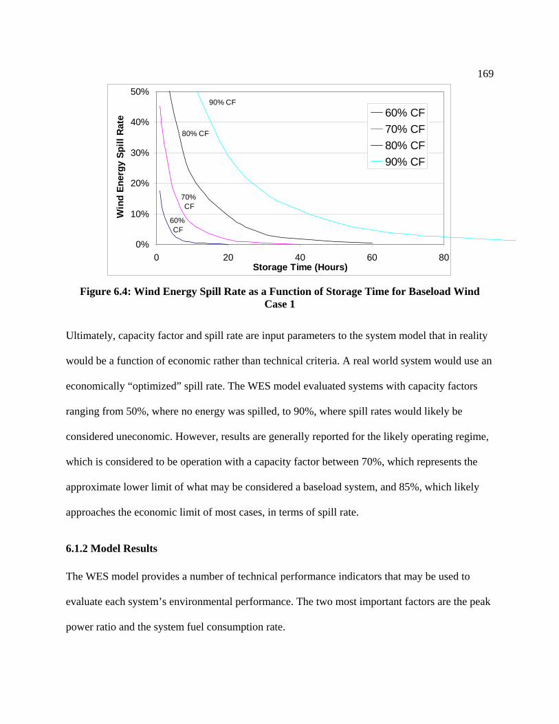
169

70% CF

80% CF

90% CF

60% CF

0%

10%

20%

30%

40%

50%

0 20 40 60 8Storage Time (Hours)

Win

d En

ergy

Spi

ll R

at

0

e 60% CF70% CF80% CF90% CF

Figure 6.4: Wind Energy Spill Rate as a Function of Storage Time for Baseload Wind

Case 1

Ultimately, capacity factor and spill rate are input parameters to the system model that in reality

would be a function of economic rather than technical criteria. A real world system would use an

economically “optimized” spill rate. The WES model evaluated systems with capacity factors

ranging from 50%, where no energy was spilled, to 90%, where spill rates would likely be

considered uneconomic. However, results are generally reported for the likely operating regime,

which is considered to be operation with a capacity factor between 70%, which represents the

approximate lower limit of what may be considered a baseload system, and 85%, which likely

approaches the economic limit of most cases, in terms of spill rate.

6.1.2 Model Results

The WES model provides a number of technical performance indicators that may be used to

evaluate each system’s environmental performance. The two most important factors are the peak

power ratio and the system fuel consumption rate.

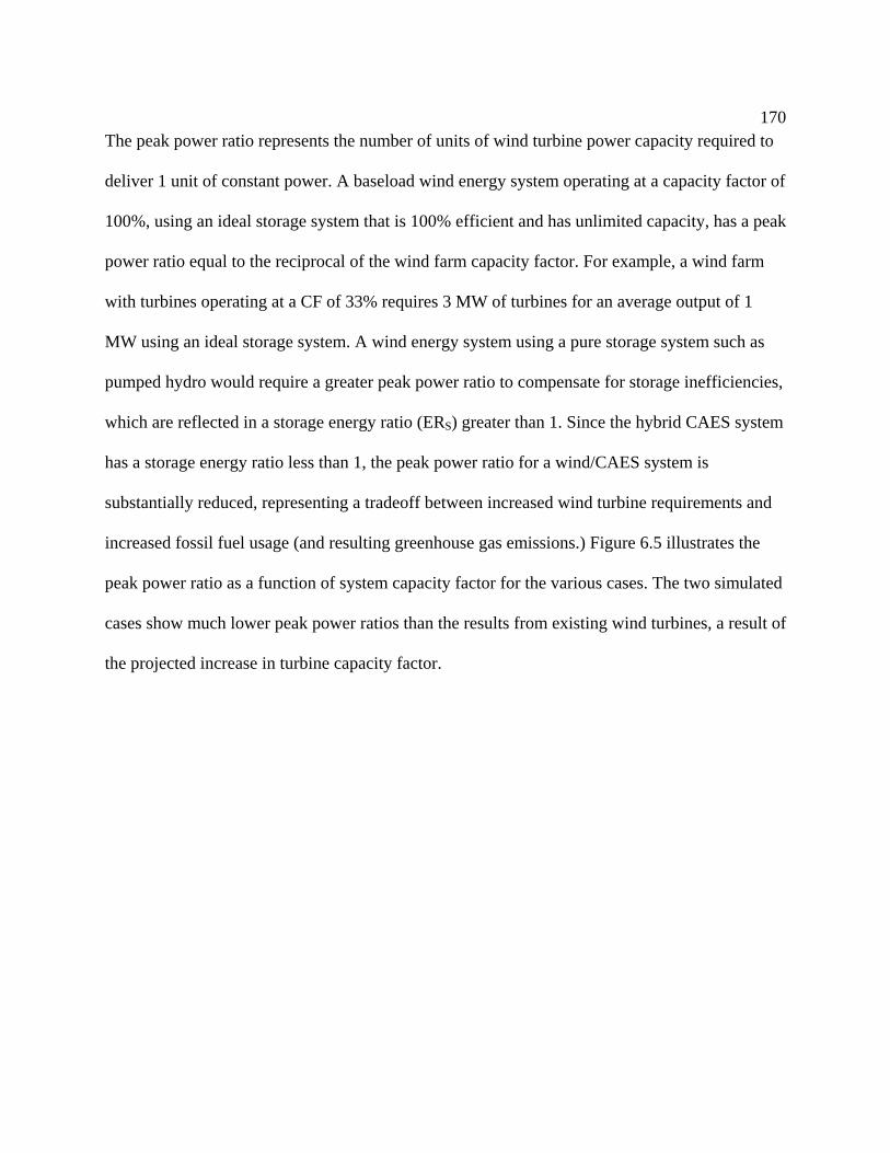
170

The peak power ratio represents the number of units of wind turbine power capacity required to

deliver 1 unit of constant power. A baseload wind energy system operating at a capacity factor of

100%, using an ideal storage system that is 100% efficient and has unlimited capacity, has a peak

power ratio equal to the reciprocal of the wind farm capacity factor. For example, a wind farm

with turbines operating at a CF of 33% requires 3 MW of turbines for an average output of 1

MW using an ideal storage system. A wind energy system using a pure storage system such as

pumped hydro would require a greater peak power ratio to compensate for storage inefficiencies,

which are reflected in a storage energy ratio (ERS) greater than 1. Since the hybrid CAES system

has a storage energy ratio less than 1, the peak power ratio for a wind/CAES system is

substantially reduced, representing a tradeoff between increased wind turbine requirements and

increased fossil fuel usage (and resulting greenhouse gas emissions.) Figure 6.5 illustrates the

peak power ratio as a function of system capacity factor for the various cases. The two simulated

cases show much lower peak power ratios than the results from existing wind turbines, a result of

the projected increase in turbine capacity factor.

171

1.01.52.02.53.03.54.04.55.0


Peak

Pow

er R

atio


Figure 6.5: Peak Power Ratio vs. Operating Capacity Factor for the Seven

Baseload Wind Cases

Figure 6.6 illustrates the system fuel consumption rate, or heat rate, defined as the CAES fuel

energy input per unit of total system output, excluding transmission effects. For systems

operating at a 70-85% capacity factor, the heat rate ranges from roughly 800- 1350 kJ/kWh, and

can be compared to a traditional fossil plant heat rate, which is typically 7,000-12,000 kJ/kWh.12

At higher capacity factors, the simulated cases demonstrate higher heat rates than most of the

existing wind farms. This is due to the simulated cases’ greater use of storage. For a given

capacity factor, the simulated cases spill less energy, and instead store it and use it in the CAES

turbine, resulting in higher fuel usage. Figure 6.6 provides additional information about system

operation. The system heat rate, divided by the constant CAES heat rate (4649 kJ/kWh,) is the

fraction of electricity ultimately provided by the storage system, which ranges from 17-29% for

the cases operating at 70-85% capacity factor.

172

0200400600800

1000120014001600


Syst

em H

eat R

ate

(kJ/

kWh)


Figure 6.6: System Heat Rate vs. Operating Capacity Factor for the Seven

Baseload Wind Cases

Table 6.2 summarizes the output parameters for various cases in their likely operating regimes

(70-85% capacity factor, using 24 hours of storage).

Table 6.2: Operational Parameters for Baseload Wind Systems Operating with a Capacity Factor of 70-85% Operational Parameter Case 1

Case 2

Range of Results for 5 Existing Wind Farms

Wind Energy Spilled (%) 1.0-12.7 0.2-6.5 3.0-31.2 Peak Power Ratio 1.4-1.9 1.4-1.7 1.8-3.4 System fuel consumption (heat) rate (kJ/kWh)

1011-1356 915-1335 783-1187

6.1.3 Environmental Assessment

The life-cycle fossil energy efficiency and greenhouse gas emissions were assessed for each case

using the operational data from table 6.2 and a component analysis of the wind and CAES

subsystems.

173

Component Analysis

This study used existing life-cycle analyses of wind energy systems to derive the energy use and

emissions associated with modern wind turbines.13,14 Life-cycle energy requirements and

emissions related to CAES and the transmission system were based on analysis performed in

chapters 4 and 5. Case 1 and the existing wind farms are assumed to use the AC transmission

line, while Case 2 uses the HVDC line. Details of the component analysis for construction and

operation of the wind/CAES system are provided in Appendix G.

Emissions and energy requirements for recharging the CAES reservoir from external sources

during low wind periods are not considered in this analysis. This is justified given the relatively

high capacity factor of the system, which is comparable to a conventional baseload plant. The net

emissions reported for most conventional systems include only emissions during operation. For

example, the net emissions from nuclear and coal-fired power plants do not include emissions

from other sources that replace their output during refueling or maintenance outages.

Fossil Fuel Efficiency

Fossil fuel efficiency is described in section 3.4.2. This measure of energy use is particularly

relevant to wind/CAES systems, since natural gas fuel is a major system input.

Fossil energy is required to construct and operate baseload wind systems. The energy related to

plant construction and decommissioning may be expressed as the total construction-related

energy, EEP (MJt), divided by the lifetime output of the storage plant EL (MWhe). The life of the

plant is assumed to be 30 calendar years. Energy for CAES fuel (natural gas) is reflected by the

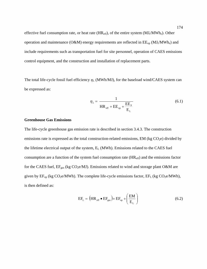
174

effective fuel consumption rate, or heat rate (HReff), of the entire system (MJt/MWhe). Other

operation and maintenance (O&M) energy requirements are reflected in EEop (MJt/MWhe) and

include requirements such as transportation fuel for site personnel, operation of CAES emissions

control equipment, and the construction and installation of replacement parts.

The total life-cycle fossil fuel efficiency ηL (MWh/MJ), for the baseload wind/CAES system can

be expressed as:

L

Popeff E

EEEEHR

1 ++

=Lη (6.1)

Greenhouse Gas Emissions

The life-cycle greenhouse gas emission rate is described in section 3.4.3. The construction

emissions rate is expressed as the total construction-related emissions, EM (kg CO2e) divided by

the lifetime electrical output of the system, EL (MWh). Emissions related to the CAES fuel

consumption are a function of the system fuel consumption rate (HReff) and the emissions factor

for the CAES fuel, EFgas (kg CO2e/MJ). Emissions related to wind and storage plant O&M are

given by EFop (kg CO2e/MWh). The complete life-cycle emissions factor, EFL (kg CO2e/MWh),

is then defined as:

( ) ⎟⎟⎠

⎞⎜⎜⎝

⎛++•=

LopgaseffL E

EMEFEFHR EF (6.2)

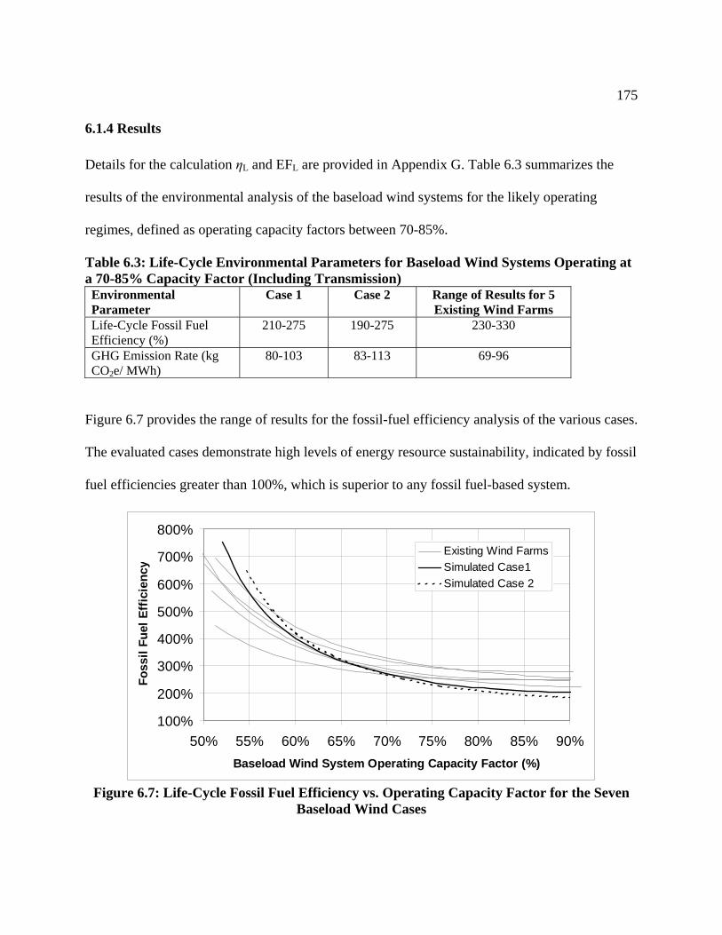
175

6.1.4 Results

Details for the calculation ηL and EFL are provided in Appendix G. Table 6.3 summarizes the

results of the environmental analysis of the baseload wind systems for the likely operating

regimes, defined as operating capacity factors between 70-85%.

Table 6.3: Life-Cycle Environmental Parameters for Baseload Wind Systems Operating at a 70-85% Capacity Factor (Including Transmission) Environmental Parameter

Case 1

Case 2

Range of Results for 5 Existing Wind Farms

Life-Cycle Fossil Fuel Efficiency (%)

210-275 190-275 230-330

GHG Emission Rate (kg CO2e/ MWh)

80-103 83-113 69-96

Figure 6.7 provides the range of results for the fossil-fuel efficiency analysis of the various cases.

The evaluated cases demonstrate high levels of energy resource sustainability, indicated by fossil

fuel efficiencies greater than 100%, which is superior to any fossil fuel-based system.

100%

200%

300%

400%

500%

600%

700%

800%


Foss

il Fu

el E

ffic

ienc

y


Figure 6.7: Life-Cycle Fossil Fuel Efficiency vs. Operating Capacity Factor for the Seven

Baseload Wind Cases

176

Figure 6.8 illustrates the distribution of fossil energy inputs for a delivered unit of electrical

energy from Case 2 when operating with an average capacity factor of 80%. Most of the energy

input is the CAES fuel, which requires about 80% of total energy input requirements when

considering both the fuel and fuel delivery.

Fuel71%

Fuel Delivery

8%Trans. Losses

10%

O&M5%

Construction6%

Figure 6.8: Distribution of Energy Sources for Baseload Wind Case 2 Operating at an 80%

Average Capacity Factor

Figure 6.9 provides the range of greenhouse gas emission rates for the various baseload wind

cases.

177

0

20

40

60

80

100

120

140


GH

G E

mis

sion

Rat

e (k

g C

O 2e

/MW

h)


Figure 6.9: System GHG Emission Rate vs. Operating Capacity Factor for the Seven

Baseload Wind Cases

The dominant source of air emissions from the wind/CAES system is natural gas combustion.

This is illustrated in Figure 6.10, the distribution of GHG emissions from Case 2 when operating

at a system capacity factor of 80%.

Construction13%

O&M6%

Trans. Losses

10%

Fuel Delivery

13%

Fuel58%

Figure 6.10: Distribution of GHG Emissions Sources for Baseload Wind Case 2 Operating

at an 80% Average Capacity Factor As can be expected, the distribution of sources is similar to Figure 6.9, since there is a general

relationship between energy use and greenhouse gas emissions. The lower fraction of emissions

178

from the CAES fuel shown in Figure 6.10 is due to the lower GHG emission rate of natural gas

compared to the higher carbon content fuels used for construction and transportation. Emissions

related to biomass clearing also increases the relative share of emissions from initial

construction.

Figures 6.8 and 6.10 shows that system fossil fuel efficiency and GHG emissions are relatively

insensitive to the parameters related to system construction and O&M. A 50% reduction in

construction-related emissions results in a life cycle GHG emissions reduction of less than 7%.

The most significant factor affecting the environmental performance of these baseload wind

systems is the consumption of natural gas fuel reflected in the heat rate. As the system capacity

factor increases, more energy is placed into storage, and consequently, more gas is burned in the

CAES turbine. This results in an increase in the greenhouse gas emission rate, and a decrease in

fossil fuel efficiency.

Substantial increases in environmental performance would require a change in the storage

system, such as an increase in the CAES turbine efficiency. Use of a storage system that does not

require fossil fuels could dramatically increase the fossil fuel efficiency and decrease the net

GHG emissions. An alternative, wind/CAES system, independent of fossil fuels, could burn

renewably-generated hydrogen, although this is probably uneconomic based on the current cost

of electrolytic hydrogen.15 Biofuels are another alternative to natural gas for the CAES system, if

CAES remains economically superior to advanced batteries or other forms of electrical energy

storage.

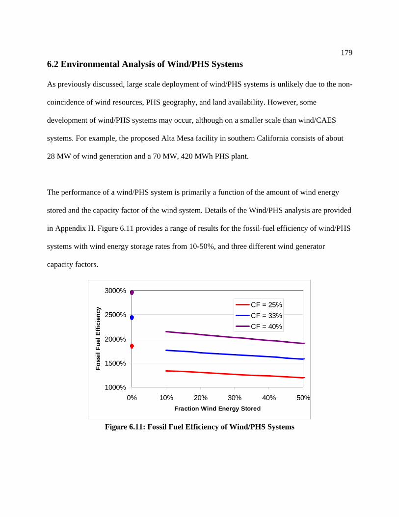
179

6.2 Environmental Analysis of Wind/PHS Systems

As previously discussed, large scale deployment of wind/PHS systems is unlikely due to the non-

coincidence of wind resources, PHS geography, and land availability. However, some

development of wind/PHS systems may occur, although on a smaller scale than wind/CAES

systems. For example, the proposed Alta Mesa facility in southern California consists of about

28 MW of wind generation and a 70 MW, 420 MWh PHS plant.

The performance of a wind/PHS system is primarily a function of the amount of wind energy

stored and the capacity factor of the wind system. Details of the Wind/PHS analysis are provided

in Appendix H. Figure 6.11 provides a range of results for the fossil-fuel efficiency of wind/PHS

systems with wind energy storage rates from 10-50%, and three different wind generator

capacity factors.

1000%

1500%

2000%

2500%

3000%

0% 10% 20% 30% 40% 50%Fraction Wind Energy Stored

Foss

il Fu

el E

ffici

ency

CF = 25%CF = 33%CF = 40%

Figure 6.11: Fossil Fuel Efficiency of Wind/PHS Systems

180

The points on the far left of Figure 6.11 (0% wind energy stored) show the fossil-fuel efficiency

of wind energy used without storage. The obvious discontinuity on the graph is due to the lack of

energy required to construct the PHS system in the non-storage case. The worst case wind/PHS

system produces more than 10 units of electrical energy per unit of fossil energy – and effective

fossil fuel efficiency of more than 1000%.

Figure 6.12 provides the range of results for the life-cycle GHG emissions over the same range

of operational parameters. It also demonstrates the substantial reduction in life-cycle emission

rate when storage is not required.

1012141618202224262830

0% 10% 20% 30% 40% 50%Fraction Wind Energy Stored

GHG

Em

issi

on R

ate

(kg

CO2e

/MW

h)

CF = 25%CF = 33%CF = 40%

Figure 6.12: Life-Cycle Greenhouse Gas Emissions of Wind/PHS Systems

6.3 Environmental Analysis of PV/BES Systems

A common proposal for solar PV is to provide peak-load generation to offset peaking power and

T&D requirements. The operation of a PV/BES system in this manner would be similar to the

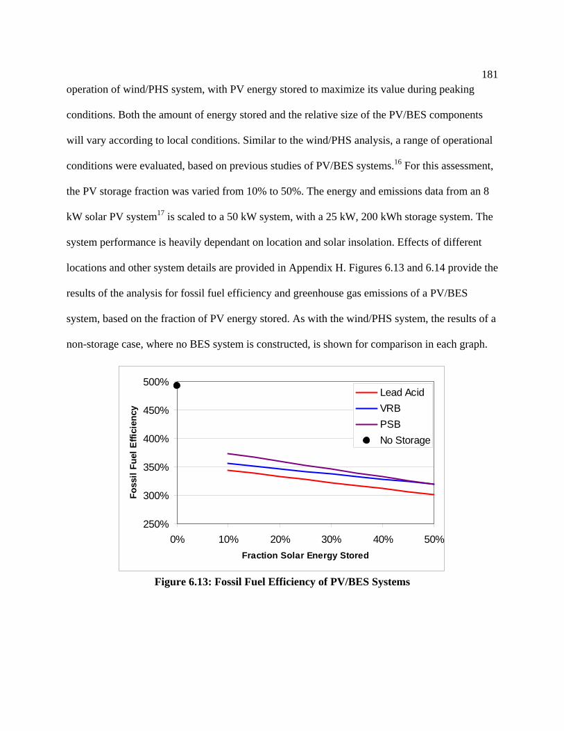
181

operation of wind/PHS system, with PV energy stored to maximize its value during peaking

conditions. Both the amount of energy stored and the relative size of the PV/BES components

will vary according to local conditions. Similar to the wind/PHS analysis, a range of operational

conditions were evaluated, based on previous studies of PV/BES systems.16 For this assessment,

the PV storage fraction was varied from 10% to 50%. The energy and emissions data from an 8

kW solar PV system17 is scaled to a 50 kW system, with a 25 kW, 200 kWh storage system. The

system performance is heavily dependant on location and solar insolation. Effects of different

locations and other system details are provided in Appendix H. Figures 6.13 and 6.14 provide the

results of the analysis for fossil fuel efficiency and greenhouse gas emissions of a PV/BES

system, based on the fraction of PV energy stored. As with the wind/PHS system, the results of a

non-storage case, where no BES system is constructed, is shown for comparison in each graph.

250%

300%

350%

400%

450%

500%

0% 10% 20% 30% 40% 50%Fraction Solar Energy Stored

Foss

il Fu

el E

ffici

ency

Lead AcidVRBPSBNo Storage

Figure 6.13: Fossil Fuel Efficiency of PV/BES Systems

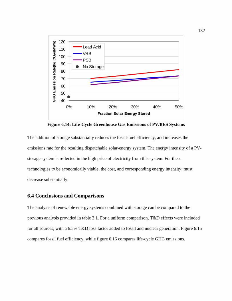
182

40

5060

70

80

90100

110

120

0% 10% 20% 30% 40% 50%Fraction Solar Energy Stored

GH

G E

mis

sion

Rat

e(kg

CO 2

e/M

Wh)

Lead AcidVRBPSBNo Storage

Figure 6.14: Life-Cycle Greenhouse Gas Emissions of PV/BES Systems

The addition of storage substantially reduces the fossil-fuel efficiency, and increases the

emissions rate for the resulting dispatchable solar-energy system. The energy intensity of a PV-

storage system is reflected in the high price of electricity from this system. For these

technologies to be economically viable, the cost, and corresponding energy intensity, must

decrease substantially.

6.4 Conclusions and Comparisons

The analysis of renewable energy systems combined with storage can be compared to the

previous analysis provided in table 3.1. For a uniform comparison, T&D effects were included

for all sources, with a 6.5% T&D loss factor added to fossil and nuclear generation. Figure 6.15

compares fossil fuel efficiency, while figure 6.16 compares life-cycle GHG emissions.

183

Data Labels are Energy Return on Fossil Investment (Efficiency/100)

0.4 0.3

16

3.46

4

17

25

0%

500%

1000%

1500%

2000%

2500%

3000%

Wind (nostorage)

Wind/PHS Wind/CAES PV (nostorage)

PV/BES Fission Gas CCGT Coal

Foss

il Fu

el E

ffici

ency

Figure 6.15: Life-Cycle Fossil-Fuel Efficiency for Electric Power Generation

(Including T&D)

7039105

2415 16

1050

500

0

200

400

600

800

1000

1200

Wind (nostorage)


PV/BES Fission Gas CCGT Coal

GH

G E

mis

sion

s (k

g C

O 2e

/MW

h)

T&DCombustionConst., O&M, Fuel

Figure 6.16: Life-Cycle GHG Emissions from Electric Power Generation (Including T&D)

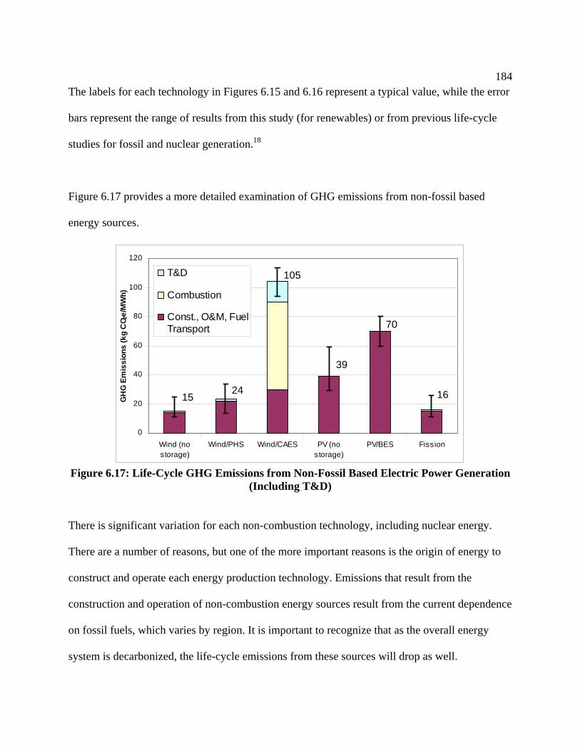
184

The labels for each technology in Figures 6.15 and 6.16 represent a typical value, while the error

bars represent the range of results from this study (for renewables) or from previous life-cycle

studies for fossil and nuclear generation.18

Figure 6.17 provides a more detailed examination of GHG emissions from non-fossil based

energy sources.

161524

105

39

70

0

20

40

60

80

100

120

Wind (nostorage)


PV/BES Fission

GH

G E

mis

sion

s (k

g C

O 2e

/MW

h)

T&D

Combustion

Const., O&M, FuelTransport

Figure 6.17: Life-Cycle GHG Emissions from Non-Fossil Based Electric Power Generation

(Including T&D)

There is significant variation for each non-combustion technology, including nuclear energy.

There are a number of reasons, but one of the more important reasons is the origin of energy to

construct and operate each energy production technology. Emissions that result from the

construction and operation of non-combustion energy sources result from the current dependence

on fossil fuels, which varies by region. It is important to recognize that as the overall energy

system is decarbonized, the life-cycle emissions from these sources will drop as well.

185

While the addition of storage substantially reduces the fossil fuel efficiency of all renewable

energy systems, their life cycle efficiency remains substantially higher than any fossil based

system. The use of natural gas fuel in CAES results in a significant difference between the two

wind/storage systems. Wind/PHS shows a fossil fuel efficiency of over 1600%, producing more

than 8 times more electricity from a unit of fossil energy than the wind/CAES system. Despite

the decrease in performance resulting from CAES operation, the least efficient wind/storage

system evaluated produces greater than 4 times more electricity per unit of fossil input than a

highly efficient combined-cycle gas turbine.

The relatively poor fossil efficiency of the PV/BES system results from the combination of

highly energy intensive generation and storage technologies.

The wind/PHS system shows emission levels that are not significantly higher (in absolute terms)

than wind without storage. The wind/CAES net emission rate of 69-113 g CO2e/kWh for the

various analyzed cases is significantly higher than the life-cycle emission rate of wind without

storage or nuclear-generated electricity. The PV/BES system’s high energy intensity is reflected

in its’ relatively high GHG emission rate, relative to other non-combustion energy sources. The

emission rate from all dispatchable renewable energy systems is substantially lower than any

fossil technology.

The use of energy storage with renewable energy systems increases their value to electric power

systems. As a result, even though their environmental performance decreases, this decrease is

186

likely offset by their increased capacity credit and system-wide impacts. As the capacity credit of

intermittent renewable energy systems is increased, they will likely displace a larger amount of

fossil-generated electricity, and provide greater overall environmental benefits, since the life-

cycle emissions rate and fuel efficiency of a renewable energy/storage system is significantly

better than any fossil fuel generator.


1 Mehta, B. (1992). CAES Geology. EPRI Journal: pp. 38-41. 2 Iowa Stored Energy Project. (2004). Via http://www.idea.iastate.edu/isep/index.asp. Accessed March 4, 2004.

3 Desai, N. and D. Pemberton (2003). Economic Value of Compressed Air Energy Storage in Conjunction with Large Scale Wind in McCamey. Ridge Energy Storage & Grid Services, LP.

4 United States. Dept. of Energy. Office of Utility Technologies. and Electric Power Research Institute. (1997). Renewable energy technology characterizations. Pleasant Hill, CA.

5 Black & Veatch. (1996) Power Plant Engineering, Chapman & Hall. 6 National Renewable Energy Laboratory. (2003) Homer V2.0. http://analysis.nrel.gov/homer/ 7 GE Wind Energy. (2003) Official Power Curves for GE Wind Energy 1.5sl, 60 Hz, Revision 2. 8 United States. Dept. of Energy. Office of Utility Technologies. and Electric Power Research Institute. (1997).

9 Minnkota Power Cooperatives. (2003) Via http://www.minnkota.com/infinity.htm. 10 McGowan, J. G. and S. R. Connors (2000). WINDPOWER: A Turn of the Century Review.

Annual Review of Energy and the Environment 25: pp. 147-197. 11 National Electric Reliability Countcil (2004) GADS database http://www.nerc.com/~gads/ 12 Elliot, T. C., K. Chen, et al.(1998) Standard Handbook of Powerplant Engineering, McGraw-

Hill.

187

13 White, S. W., and G. L. Kulcinski (2000). Birth to Death Analysis of the Energy Payback

Ratio and CO2 Gas Emission Rates from Coal, Fission, Wind, and DT Fusion Electrical Power Plants,. Fusion Engineering and Design 48(248): pp. 473-481.

14 Schleisner, L. (2000). Life cycle assessment of a wind farm and related externalities.

Renewable Energy 20: pp. 279-288. 15 Padró, C. E. G. and V. Putsche (1999). Survey of the Economics of Hydrogen Technologies.

National Renewable Energy Laboratory. Golden, Colorado. NREL/TP-570-27079. 16 Marwali (1998). Short term generation scheduling in photovoltaic-utility grid with battery

storage. IEEE Transactions on Power Systems. 13(3): pp. 1057-1062. 17 Meier, P. J. and G. L. Kulcinski (2002). Life-Cycle Energy Requirements and Greenhouse Gas

Emissions for Building-Integrated Photovoltaics. Energy Center of Wisconsin Research Report 210-1.

18 Gagnon, L., et al. (2002). Life-cycle assessment of electricity generation options: The status of

research in year 2001. Energy Policy 30(14): pp. 1267-1278.

188

7. Environmental and Policy Assessment of Energy Storage used with Fossil Sources

The analysis in Chapter 4 found that electricity delivered from energy storage when coupled to

low-carbon energy sources, such as nuclear and renewable energy, produces far less GHG

emissions than fossil generation sources. Chapter 6 demonstrated that integrated renewable

energy/storage systems also deliver relatively low levels of carbon emissions. While these results

indicate that energy storage may be an effective tool in lowering carbon emissions from

electricity generation, near term applications of energy storage may not have a net positive

impact on carbon emissions, or emissions of harmful air pollutants.

The proposed Norton CAES plant is designed to use inexpensive, off peak coal generation, and

resell this energy at times of higher demand. This application raises an interesting question of

how the effective emissions from this plant should be measured and regulated. Any conventional

generator must meet certain clean air standards which are different (generally more stringent)

than those applied to existing plants. Energy storage appears to be able to take advantage of a

loophole in federal regulation regarding the construction of new power plants.

This chapter provides an overview of the U.S. Clean Air Act, and examines the regulations that

affect the use energy storage with existing power plants. It also provides an analysis of the actual

emissions that will result from the construction and operation of energy storage facilities,

compared to conventional alternatives. This chapter also proposes and evaluates policies that will

189encourage storage to be used to assist, rather than hinder the progress towards improved air

quality.

7.1 Evaluation of the U.S. Clean Air Act Applied to Energy Storage

An energy storage facility can be regarded as an electric power plant with several unique

characteristics, including its geographical and temporal displacement of air emissions. Most or

all of their effective emissions are produced at another location, and there are no federal

regulations that specifically address the interaction between energy storage and existing

facilities. The emissions created by the use of energy storage originate from existing power

plants with spare capacity. These plants are regulated by various provisions of the U.S. Clean Air

Act, including the New Source Review program.

7.1.1 Basic Provisions of the Clean Air Act and New Source Review

The U.S. Congress has passed a number of laws designed to reduce air pollution and improve

national air quality. The most important of these laws are embodied in the Clean Air Act (CAA),

and its amendments. In 1970 the CAA established national ambient air quality standards

(NAAQS), which establish upper limits for the ambient concentration of six “criteria” pollutants:

sulfur dioxide (SO2), nitrogen oxides (NOx), carbon monoxide (CO), lead (Pb), particulate matter

(PM), and ground-level ozone (O3).1 Each state is responsible for establishing a State

Implementation Plan to ensure that these air quality standards are met in each geographic area in

the state.2

In 1977 the CAA was amended, to establish a two-track system for addressing air quality

standards. The first set of rules addresses “non-attainment” areas, which do not meet NAAQS.3

190The second set of rules establishes Prevention of Significant Deterioration (PSD) program,

which addresses areas in attainment, where air quality does meet NAAQS.4

A major component of both tracks is the New Source Review (NSR) program that establishes

specific rules regulating emissions from large stationary sources, such as electric power plants.5

This program regulates the construction and operation of electric power facilities that have the

potential to annually emit more than 100 tons of a regulated pollutant.6

When new major emission sources are proposed, pre-construction permits must first be obtained

from the state permitting authority, which oversees the requirements of the federal CAA

standards, including those of the NSR program.7 Application for a permit must be accompanied

by a technical evaluation of the projected emissions from the plant, including models of possible

distribution of pollution concentration, and qualifications of other potential impacts on human

health and the environment.8

The NSR program also contains technical standards referred to as New Source Performance

Standards (NSPS) that establish emissions rates and emissions control equipment that must be

installed on new plants. The NSPS depend on type and size of plant, and also on existing local

air quality. If the area is in attainment, then the new source must conform to PSD rules.9 In this

case, the utility must install “best available control technology” (BACT) to control its emissions

of each of the six criteria pollutants.

191If the proposed plant is in an area not in attainment, then stricter rules are required for a new

plant. Instead of BACT, the proposed facility must install technology that achieves “lowest

achievable emission rate” (LAER.)10 In addition, the facility’s emissions must be offset by

emission reductions from other facilities in the area.11

It should be noted that NSPS are input-based emission standards as opposed to output-based

standards. The standards establish the amount of emissions that are allowed per unit of fuel

burned, not per unit of electricity produced. As a result, there is no defined standard for the

amount of pollutants produced per unit of electricity generated. Input-based standards also

provide little incentive for increased efficiency, nor substantial penalties for low efficiency.

Determining the actual “emission standard” for a new plant is complicated by the technology

requirements. Technology requirements such as BACT generally create more stringent emission

standards than NSPS. For example, current NSPS allows for up to 0.6 lb or 1.2 lb of SO2

emissions for each MMBTU of fuel input, depending on fuel type.12 The standards also require

BACT for SO2, which includes a number of flue-gas desulfurization technologies, generally

referred to as scrubbers. The actual scrubber types that are allowed by the EPA must achieve

specific SO2 emission reduction rates of at least 70% or 90%, again depending on fuel type. The

effective result of the current BACT standards is a maximum input emission rate generally

between 0.06 and 0.32 lb SO2/MMBTU, depending on fuel sulfur content. As a result, the

technology standards render the NSPS emission standards irrelevant, and further complicate the

process of attempting to precisely identify the legally required emission rates for electric

192generators affected by NSR. Some state and federal regulations for electric power plants

include output-based standards, but the majority of CAA regulations continue to be based on fuel

input.

When Congress was developing rules for new sources, they were faced with the issue of how to

deal with existing plants, whose emissions often greatly exceeded NSR standards. In areas where

local NAAQS are not met, states must develop plans that may include retrofits on existing

facilities.13 However, it was recognized that requiring immediate retrofit of all of the nation’s

generation facilities, especially those in areas that already meet NAAQS standards, would be

economically disruptive.14 It was decided that existing facilities in attainment areas would be

allowed to continue to emit at their existing high level emission rates, until the facilities were

upgraded or otherwise modified, at which point they would be considered new sources, and

required to meet NSR rules. This decision, known as grandfathering, is probably the most

controversial and contentious aspect of the New Source Review program.

While there is no “sunset” provision for these grandfathered power plants, it is generally

concluded that Congress believed that power plants, like any technology, have limited lifetimes,

and would eventually be replaced.15 In addition, it is suggested that Congress viewed the

generation of electric power like other industries – that improved technology would force the

upgrade of existing plants to remain competitive. As a result, it is generally believed that

Congress thought that older plants would eventually be retired or upgraded out of economic

necessity. New construction or major upgrades provide the most economic opportunity for

installation of new pollution equipment, so NSR is triggered for existing plants at the time of a

193major modification. This rule, referred to as the “change rule” in this chapter, states that NSR

shall be triggered by:

any physical change in, or change in the method of operation of, a stationary source which increases the amount of any air pollutant emitted by such source or which results in the emission of any air pollutant not previously emitted.16

Despite the fairly clear language, this terminology is insufficient to guide an operating utility.

Terms such as “physical change” and “method of operation” must be sufficiently defined for a

utility to follow the rules. Since enactment of the CAA, federal agencies have attempted to

clarify the change rule to more precisely define these terms. These decisions have a significant

impact on the use of energy storage with existing facilities.

7.1.2 The EPA’s Attempts to Clarify the New Source Review Provisions Regarding Existing Facilities The Administrative Procedures Act (APA) of 1948 grants federal agencies certain powers to

draft rules and regulations in order to accomplish the stated goals of Congressional legislation.17

The Clean Air Act is an example of an “enabling act” which creates a new program, with

specific goals. The APA establishes the authority of a designated agency (in this case the

Environmental Protection Agency) to implement specific rules and regulations to effectively

achieve legislative goals. This allows the necessary specific technical details of regulation to be

developed by experts, as opposed to Congress, whose members may lack the necessary

background to implement complicated technical programs.

The administering agency often has the responsibility of creating rules to achieve legislative

goals for specific circumstances that have not been completely defined by the legislature. The

194specific, technical definition of “physical change” in the CAA is an example. The EPA must

conform, as much as possible, to Congressional intent when defining this term. The

“reasonableness” of agency rulemaking is often the subject of considerable scrutiny and

litigation.

The responsibilities and constraints of the EPA with regard to this type of rulemaking were

addressed by the Supreme Court in 1984.18 The court decision in Chevron v. Natural Resources

Defense Council, Inc established a two-step test (often referred to as the Chevron test) for

determining the legality of agency rulemaking. First, Congressional intent must be established:

“If the intent of Congress is clear, that is the end of the matter; for the court, as well as the

agency, must give effect to the unambiguously expressed intent of Congress.”19 Second, if intent

is unclear or not sufficiently defined, deference must be given to the agency, and a court is

limited in its ability to create its own rules: "a court may not substitute its own construction of a

statutory provision for a reasonable interpretation made by the administrator of an agency."20

The court explains its decision by stating that public policy, if unaddressed by Congress

specifically, is better decided by an administering agency, which has both greater expertise and

greater public accountability than the courts.

Judges are not experts in the field, and are not part of either political branch of the Government. Courts must, in some cases, reconcile competing political interests, but not on the basis of the judges’ personal policy preferences. In contrast, an agency to which Congress has delegated policy-making responsibilities may, within the limits of that delegation, properly rely upon the incumbent administration’s view of wise policy to inform its judgments. While agencies are not directly accountable to the people, the Chief Executive is, and it is entirely appropriate for this political branch of the Government to make such policy choices – resolving competing interests

195which Congress itself either inadvertently did not resolve, or intentionally left to be resolved by the agency charged with the administration of the statute in the light of everyday realities.21

This rule, while simple in principle, does not necessarily simplify implementation of the CAA, or

the change rule. Since initial passage of the CAA, the EPA has promulgated a number of rules

attempting to define “physical change.” Many have been challenged, because for NSR, both

“tests” established by the Chevron ruling do not provide clear answers. In most challenges to

EPA rule making, both sides have claimed fairly clear Congressional intent in their favor, and

also have claimed that rules promulgated by the EPA have not provided a “reasonable

interpretation” of Congressional intent.

The EPA’s first attempt to provide a definition of “physical change” was a rule that defined a

“change” as resulting in an annual increase of 100 or 250 tons per year of any regulated

pollutant, depending on the source category.22 The EPA also provided several categorical

exemptions from the definition of physical change, including “routine maintenance and repair.”

In 1979 several of the EPA’s rules were challenged, and the court in Alabama Power v. Costle

rejected the “annual increase” definition of change, stating “EPA has extremely limited authority

to exempt activities from the definition of ‘modification’. . . . The Agency’s authority is limited

to circumstances of administrative necessity and circumstances having a ‘de minimis’ or ‘trivial

impact on emissions.”23 The court also stated “[T]he term ‘modification’ is nowhere limited to

physical changes exceeding a certain magnitude.”24

196The ruling did not address the various exemptions, nor did it help establish clear limitations

on what modifications may occur, and it left industry with little additional guidance. Since this

ruling, the EPA has made several attempts to clarify these rules, with limited success, and the

change rule as of 2004 is still only defined by what it is not, established by a number of

exemptions.25 Major exemptions to the “change rule” include:

1) Routine maintenance, repair, and replacement

2) Increase in production rate, if unaccompanied by capital expenditure

3) An increase in the hours of operation

4) Use of alternate fuels

5) Installation of new pollution control equipment

The most important of these exemptions for energy storage is the “hours of operation”

exemption, which establishes the legal use of energy storage without triggering new source

review.

7.1.3 The Hours of Operation Exemption and Energy Storage

The hours of operation exemption has a clear impact on the use of electricity storage. An energy

storage facility may store off-peak power from an older coal plant in an area currently in

attainment, substantially increasing the hours of operation of this plant, and consequently, its air

emissions. As long as NAAQS standards are not exceeded, the increase in emissions and

potential decrease in air quality that result from the use of energy storage is allowed due to the

hours of operation exemption.

197It is important to consider, however, whether or not the hours of operation exemption was

intended to allow for significant increases in emissions that are not the result of demand

variations. In many ways the hours of operation exemption appears reasonable. Electric demand

is highly variable, largely uncontrollable, and somewhat unpredictable. While utilities can

roughly estimate the expected annual increases in electric demand, it would be impossible for

them to predict exactly how much a plant will need to produce from year to year, especially

considering the effects of weather-related demand. It is probably not reasonable for NSR to be

triggered if a residence turns on an extra light bulb and increases the demand on a utility’s

intermediate load coal plant. Implementation of NSR is expensive and time consuming, and it is

not practical for utilities to address small uncontrollable changes in demand through the NSR

processs. The EPA recognized this limitation and justified the hours of operation exemption by

stating “Congress could never have intended a company to have to obtain an NSR permit before

it could lawfully change hours or rate of operation.”26

The use of energy storage, however, is unlike daily, seasonal, and yearly variations in demand,

many of which are fairly unpredictable. Use of energy storage is a planned business action that

would likely require long term purchase contracts between the generator and the storage facility.

In other words, the generator would know ahead of time that an increase in output (and

emissions) was anticipated.

As a result, the use of energy storage would not necessarily be external to the operation of the

generating plant – there must be a synergistic relationship between the ability of the plant to

198increase output, and the requirements of the energy storage facility. This difference could be

deemed “controllable” vs. “uncontrollable” load growth.

This potential difference has been previously noted by legal scholars who have questioned the

legality of the hours of operation exemption under certain circumstances similar to the use of

energy storage (but not referring directly to its use).

when a utility makes a long-term, strategic decision to increase the utilization of a power plant from 30 percent on average to 60 percent on average over an extended period, it is hard to understand why this is not an “operational change.” Such a change, if accompanied by a significant emissions increase, would appear to require the NSR under the statutory definition of “modification.” 27

From another perspective, it is reasonable to ask why Congress would include the term “change

in the method of operation” in the law if it did not intend to address long-term, strategic

decisions such as the use of energy storage. It is reasonable then to consider that a planned

business decision to increase output and turn an intermediate load plant into a baseload plant via

the use of energy storage might be a “change in the method of operation” as defined by

Congress. Furthermore, such a change clearly “increases the amount of any air pollutant emitted

by such source.” As a result, it is possible that the hours of operation applied to the use of energy

storage is outside the bounds of “administrative necessity and circumstances having a ‘de

minimis’ or ‘trivial impact on emissions’” which is the intent of Congress, as interpreted by the

court in Alabama Power v. Costle.

1997.1.5 New Source Review and On-Site Energy Storage

The “reasonableness” of the hours of operation exemption applied to energy storage can be

further examined by considering a hypothetical application: a large storage plant constructed on-

site and physically attached to an existing fossil-based power plant. While such a plant has not

been built since passage of the CAA, an examination of NSR interpretation and enforcement

action by the EPA tends to reinforce the view that the use of energy storage is an unreasonable

application of the “hours of operation” exemption.

The CAA change rule establishes that NSR is triggered by two “events” at a major facility: first,

a physical change, or change in method of operation must occur, and second, there must be a

significant increase in emissions.

As discussed in section 7.1.4, the only definition of physical change in EPA rules is what it is

not, based on exemptions. It is unlikely that an energy storage facility could be interpreted in any

of the three “physical” exemptions. Energy storage is not a replacement or repair, it does not

allow for alternative fuels to be burned, and it is unlikely to be interpreted as a pollution control

project.

A utility would likely claim that an energy storage facility is a “stand-alone” addition to a plant,

which does not trigger NSR for the existing source. (For example, an addition of a second boiler

to an existing plant does not result in the first boiler being subject to NSR.) A utility would likely

claim that an on-site energy storage facility would be exempted. However, this exemption

assumes that the new equipment does not somehow interact with the first, which is not the case

200for energy storage. The precedent is established by the second part of the test, a

determination if there is an increase in emissions as a result of the physical change.

The EPA has proposed several rules to establish the measurement of post-change emissions, and

this issue has been litigated a number of times. The EPA originally promoted an “actual to

potential” test, which compares historical annual emissions to potential emissions that would

result if the plant were to run constantly at full capacity. This test was struck down by the court

in Wisconsin Electric Power (WEPCO) v. Reilly,28 which is reasonable considering the actual to

potential test will always result in a theoretical increase in emissions, since no plant can operate

at full capacity at all times.

After the WEPCO ruling, the EPA promulgated the “actual to projected actual” test (referred to

as part of the “WEPCO rule”) that compares the actual annual emissions in the two years before

the physical change, to the likely actual annual emissions after the physical change. An onsite

energy storage facility would result in increased annual output, and based on the WEPCO rule, it

appears likely that the use of on-site storage would trigger NSR.

This WEPCO rule has been the basis for recent EPA actions again power plant owners that have

performed upgrades on coal-fired power plants. After the WEPCO rule was established, the EPA

began investigation of suspected NSR violations. In 1999 and 2000, the Department of Justice

filed eight actions on behalf of the EPA against utilities for CAA violations.29 Recent court

opinions in these cases provide additional insight into the potential legality of on-site energy

201storage, as they specifically address the hour of operation exemption rule, when accompanied

by a physical change to the facility.

One of the EPA suits in 1999 was against Ohio Edison, claiming that eleven construction

projects at its large Sammis coal-fired power plant were significant modifications that resulted in

increased emissions. While the projects did not involve energy storage, a primary purpose of the

Sammis projects was to “prevent or at least diminish the number and duration of outages,

meaning unplanned periods of time when the unit was offline and unproductive.”30 This means

that the work was not intended to increase the rate of production, but to increase the number of

hours of availability.

Ohio Edison’s defense included two major points: first, that the routine maintenance, repair, and

replacement (RMRR) exclusion applied, and second, even if the modifications were major, they

were still exempted because the emission rate did not increase. The increased hours of

availability that resulted from the project resulted only in increased hours of operation, which is

specifically exempted from NSR. This argument could be applied to the addition of energy

storage, as it results in an increased number of hours per year that the plant produces saleable

electricity.

The court rejected the RMRR exclusion, concluding that the projects were not routine. More

importantly for energy storage, the court took a narrow view of the hours of operation

exemption, stating that the exclusion in this case is not applicable under the new WEPCO rule:

202The language of this regulation clearly creates an exemption to the definition of "physical change" that applies when there is an increase in hours of operation unaccompanied by physical construction to the unit itself. For example, the exemption applies when there is a temporary increase in electricity demand which, without a physical change at a unit, results in an increased output of electricity. See WEPCO, 893 F.2d at 916, citing 45 Fed.Reg. 52676, 52704 (1980).31

Furthermore, the court specifically addresses modifications that allow increased annual output,

which would directly be applicable in the case of on-site energy storage:

[T]he [Ohio Edison] projects were all intended to result in increased hours of operation as a result of a reduction in the number and length of forced outages, or shutdown for repair or maintenance. A significant decrease in outages results in a significant increase in both production and emissions. Given the actual goals placed on the construction projects by Ohio Edison, and the substantial increase in emissions certain to follow, the company was required to project future emissions. If those projected increases were substantial, as defined by regulations noted below, preconstruction approval, which was never sought, was required by law.32

The basic conclusion of the Ohio court is fairly straightforward: a physical modification,

accompanied by an increase in annual emission rate, is subject to NSR regulation, as established

by the WEPCO rule.

It should be noted however, that the new WEPCO rule for determining post-modification

emission rates has not been universally accepted by the courts. In an NSR case very similar to

the Ohio Edison case, the court in United States v. Duke Energy Corp. ruled that the older hours

of operation exemption cannot be invalidated by the newer WEPCO rule without sufficient

justification, which according to the court, is not provided.33 In this case, the court does not defer

to the agency and claims that the intent of Congress has clearly allowed the hours of operation

exemption to remain, since it did not address the issue in the 1977 or 1990 amendments to the

CAA. The court essentially agrees with the defendant in the Ohio Edison case, that while a

203modification may not be exempted, if the result is only an increase in hours of operation, than

this is exempted. (The court does, however, agree that an increase in emissions rate would

trigger NSR.)

Both the Ohio Edison and Duke Energy courts quote various interpretations of the hours of

operation exemption made by various EPA officials over the years, with opinions often a

function of the political leanings of the current administration.

While the resolution of the applicability of the hours of operation exemption may lie with a

higher court, it appears reasonable that the onsite use of energy storage would be interpreted as a

physical change, resulting in increased emissions. This conclusion reinforces the idea that off-

site energy storage, coupled with existing plants, is a loophole in NSR, since an energy storage

device can be a physical modification to an existing plant, which is attached not with pipes and

valves, but with electric wires. A utility considering energy storage would likely avoid

constructing the facility on-site to avoid triggering NSR, but instead could locate the facility a

short distance away, and couple the two facilities via transmission. These two applications, while

having the exact same results from an engineering and emission standpoint are treated differently

by existing policy.

7.1.6 Recent Administration Actions on New Source Review and Their Impact on Energy Storage The EPA under the administration of President Bush has made several attempts to modify New

Source Review that could have some impact on the use of energy storage.

204On December 31, 2002, the EPA promulgated a new rule that revises the WEPCO “actual to

potential actual” test.34 Of most concern to environmentalists was the change in baseline for

measuring pre-modification emissions levels. The older rule used emissions measured over the

24 months prior to the modification as the baseline, while the new rule allows the baseline

measurement to occur over any 24 month period in the last 10 years. This weakens the previous

rule by allowing a utility to use the “dirtiest” 24 month period as a baseline. The new rule did,

however, continue the use of an annual emission rate, instead of an hourly emission rate, when

considering the change. This tends to reinforce the notion that the EPA recognizes that annual

emissions are a better measure of actual impact than hourly rates. In defending its decision to

keep annual emissions in the new test, the EPA states:

[The EPA] also expressed concern about the environmental consequences associated with the Exhibit B provisions [which measured only hourly rates, and not annual rates]. For one, you could modernize your aging facilities (restoring lost efficiency and reliability while lowering operating costs) without undergoing preconstruction review, while increasing annual pollution levels as long as hourly potential emissions did not change.35

This new rule would tend to reinforce the conclusion in the Ohio Edison case that considers

annual emission rates the more important factor in measuring change.

Of far greater concern to environmentalists, and having potentially more impact on the actual use

of energy storage is the rule promulgated on August 27, 2003.36 This rule is a modification of the

RMRR exclusion rule, and represents a significant change to the EPA’s interpretation of NSR

The rule allows any plant operator to perform any modification to the plant, as long as the cost of

the modification does not exceed 20% of the value of the plant. More importantly, the rule places

205no restriction on the number of modifications that may be performed over an extended time

period. This rule would appear to allow the complete reconstruction of a plant, one 20% at a

time, without ever triggering new source review.

While neither of these new rules directly addresses the legality of energy storage, they do make

energy storage easier to implement in practice. Before these rules were proposed, a plant

operator may have been unable to increase annual plant output due to the need for plant upgrades

that may have triggered NSR. The new 20% rule now allows for extensive upgrades, which

could be performed for the express purpose of increasing plant availability in order to sell to a

new merchant storage facility. These upgrades can be performed without triggering new source

review and the storage facility can sell energy that produces emissions that greatly exceed NSPS,

while any competitive new source of generation must meet NSPS.

The modification rules were perceived by many environmentalists as a complete “rollback” of

NSR, and quickly challenged in court by several states.37 On December 24, 2003, the D.C.

Circuit Court of Appeals halted implementation of the rules.38 The de minimus ruling in

Alabama Power v. Costle appears to challenge the ability of the EPA to create such categorical

exemptions such as the greatly expanded RMRR rule, but the new rules have certainly set the

stage for another round of courtroom challenges that will likely take many years to resolve.

7.1.6 Conclusions

Some interpretations of NSR make a compelling case that the use of energy storage is an

unjustified application of the hours of operation exemption. Alternately, a strict interpretation of

206the hours of operation exemption would allow the use of energy storage with existing power

plants, even if constructed on-site, and resulting in considerable increases in emissions. The

disparate viewpoints taken in recent litigation involving existing and proposed EPA rules have

led some observers to suggest that the definition of “any physical change in, or change in the

method of operation…. which increases the amount of any air pollutant” may ultimately lie

with the Supreme Court’s interpretation of Congressional intent.

While a complete analysis of Congressional intent regarding NSR is beyond the scope of this

work, a few observations can be made about the use of energy storage and new source review:

1) The nature of electricity means that a “physical change” to a power plant may occur at a

location some distance from the plant.

2) The long term contracts associated with the planned use of energy storage could

reasonably be interpreted as a “change in the method of operation”

3) While the hours of operation exemption seems reasonable for unplanned and

uncontrollable demand growth, it is less reasonable when applied to the planned use of

energy storage.

4) Many of the rules established in the CAA specifically address emissions in yearly

amounts and hourly emission rates. Congress recognized that both measurements of

emissions are important to protect human health and the environment. Allowing large

annual increases of emissions through the hours of operation exclusion is incompatible

with this viewpoint.

5) The “de minimus” ruling of Alabama v. Costle implies that the court considers an annual

increase of 100 or 250 tons to be greater than an acceptable value, and beyond the intent

207of Congress. This ruling appears to be incompatible with the hours of operation

exemption, especially considering this exemption may produce an annual increase at a

plant that is much higher than this value.

6) The hours of operation exclusion does little to protect the health and welfare of the

citizens of the U.S., while at the same time it provides substantial distortion of the

marketplace. It allows incumbent utilities to use low cost, high emissions electricity with

storage to compete with new sources that must bear the costs of NSR.

The potential effects of the energy storage loophole can be evaluated by measuring the emission

rates and annual emissions that may result from the use of energy storage systems with existing

coal-fired power plants.

7.2 Emissions Resulting from the Use of Storage Systems with Coal Fired Power Plants This chapter suggests that energy storage systems should be viewed as a new source of peaking

and load following electricity, and that net air emission impacts should be analyzed from that

perspective. To perform this analysis, it is necessary to understand in detail the sources of stored

energy, as well as the interaction between energy storage and fossil energy sources.

7.2.1 Availability Generation for Energy Storage Systems

The suggestion that the use of energy storage represents a loophole in the CAA implies that there

is a great deal of unused capacity from existing grandfathered power plants. If this is not true,

this “loophole” will be of little consequence to actual increases in air emissions. A power plant

survey was performed to identify the availability of off-peak coal-based generation. This was

208performed by comparing the actual production of the nation’s coal plants to their potential

output if used at maximum capacity.

Since the bulk of the existing coal generation capacity is in near the industrial Midwest, and

since the largest proposed CAES plant is located in Ohio, coal plants in the six state region

around Ohio, including Michigan, Indiana, Kentucky, West Virginia, and Pennsylvania, were

evaluated. Actual annual production data was derived from the EPA’s E-Grid database39 for the

year 2000 for each plant. The actual production data was then compared to their maximum

potential output, based on average availability for plants in each class (size) of plants, derived

from the National Electric Reliability Council (NERC) Generating Availability Data System

(GADS) database.40 The total difference provides an approximate idea of how much spare

capacity exists in the coal-fired power plants in this region.

The facilities evaluated were dedicated electric generation facilities, and excluded cogeneration

facilities, small plants (under 25 MW), and plants with very low (<5%) capacity factors.

Overall, there are a total of 111 plants meeting these criteria, with a total capacity of about 104

GW. In 2000, these plants generated with an average capacity factor of 61%, while the average

availability of these plants was 82-86%, with a capacity weighted average of about 84%,

according to the GADS database. The difference between actual and potential generation is a

potential increase of roughly 205,000 GWh, equivalent to about 28 GW (28 large plants) of

“new” baseload generation operating at 84% CF. There is clearly significant capacity available

for energy storage in this region.

2097.2.2 Emission Rates of Existing Coal-Fired Generators

The EPA E-Grid database was used to evaluate emissions from existing sources that may provide

electricity to energy storage facilities. There is considerable variation in the emission rates of

CO2, SO2, and NOx, among these older plants. The CO2 emission rate is a direct function of the

overall thermal efficiency (heat rate) of the plant. The emissions of SO2 are a function of both

heat rate and coal sulfur content, which varies from about 0.3-1.5% for “low sulfur” western

coal, to 3-4% for high sulfur eastern coal.41 Most grandfathered plants do not use SO2 scrubbers,

which are currently required by NSR regulations. NOx emissions are a function of heat rate and

the combustion characteristics of the power plant. Most existing plants use “low NOx” burners,

but do not employ post-combustion controls, such as selective catalytic reduction (SCR), which

is required by NSR for new plants. Modern plants meeting NSPS have several additional

environmental benefits due to increased thermal efficiency, including lower thermal pollution,

reduced fine particulate emissions, and lower mercury emissions. Prior to 2004 mercury was

unregulated, but in 2004 the EPA proposed a cap-and-trade system to control mercury

emissions.42

Appendix I provides additional details of availability and emissions rates of representative plants

that can be used to provide off-peak electricity for the use of energy storage. Table 7.1 provides a

summary of typical rates for high, low and average emission rates for existing grandfathered

plants, as well as rates for more contemporary plants. Emission rates are based on fuel inputs and

are expressed in English units (lbs. and BTU) since these are the units used by reporting agencies

and codifed in federal law.

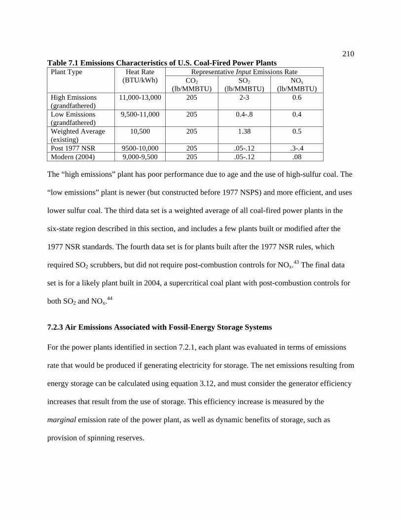
210Table 7.1 Emissions Characteristics of U.S. Coal-Fired Power Plants

Representative Input Emissions Rate Plant Type Heat Rate (BTU/kWh) CO2

(lb/MMBTU) SO2

(lb/MMBTU) NOx

(lb/MMBTU) High Emissions (grandfathered)

11,000-13,000 205 2-3 0.6

Low Emissions (grandfathered)

9,500-11,000 205 0.4-.8 0.4

Weighted Average (existing)

10,500 205 1.38 0.5

Post 1977 NSR 9500-10,000 205 .05-.12 .3-.4 Modern (2004) 9,000-9,500 205 .05-.12 .08

The “high emissions” plant has poor performance due to age and the use of high-sulfur coal. The

“low emissions” plant is newer (but constructed before 1977 NSPS) and more efficient, and uses

lower sulfur coal. The third data set is a weighted average of all coal-fired power plants in the

six-state region described in this section, and includes a few plants built or modified after the

1977 NSR standards. The fourth data set is for plants built after the 1977 NSR rules, which

required SO2 scrubbers, but did not require post-combustion controls for NOx.43 The final data

set is for a likely plant built in 2004, a supercritical coal plant with post-combustion controls for

both SO2 and NOx.44

7.2.3 Air Emissions Associated with Fossil-Energy Storage Systems

For the power plants identified in section 7.2.1, each plant was evaluated in terms of emissions

rate that would be produced if generating electricity for storage. The net emissions resulting from

energy storage can be calculated using equation 3.12, and must consider the generator efficiency

increases that result from the use of storage. This efficiency increase is measured by the

marginal emission rate of the power plant, as well as dynamic benefits of storage, such as

provision of spinning reserves.

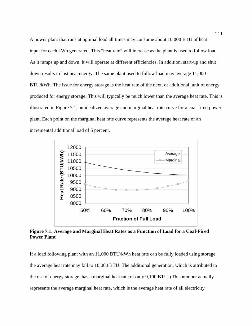
211A power plant that runs at optimal load all times may consume about 10,000 BTU of heat

input for each kWh generated. This “heat rate” will increase as the plant is used to follow load.

As it ramps up and down, it will operate at different efficiencies. In addition, start-up and shut

down results in lost heat energy. The same plant used to follow load may average 11,000

BTU/kWh. The issue for energy storage is the heat rate of the next, or additional, unit of energy

produced for energy storage. This will typically be much lower than the average heat rate. This is

illustrated in Figure 7.1, an idealized average and marginal heat rate curve for a coal-fired power

plant. Each point on the marginal heat rate curve represents the average heat rate of an

incremental additional load of 5 percent.

8000850090009500

1000010500110001150012000

50% 60% 70% 80% 90% 100%

Fraction of Full Load

Hea

t Rat

e (B

TU/k

Wh) Average

Marginal

Figure 7.1: Average and Marginal Heat Rates as a Function of Load for a Coal-Fired Power Plant

If a load following plant with an 11,000 BTU/kWh heat rate can be fully loaded using storage,

the average heat rate may fall to 10,000 BTU. The additional generation, which is attributed to

the use of energy storage, has a marginal heat rate of only 9,100 BTU. (This number actually

represents the average marginal heat rate, which is the average heat rate of all electricity

212produced raising the power plant from partial to full load.) This efficiency gain is realized

only because of the decreased cycling that results from the use of energy storage and can

potentially produce lower emission rates from existing sources, particularly compared to

relatively inefficient load-following alternatives.

The heat rate curves for individual power plants are generally not available. In addition,

published heat rate curves do not include the efficiency losses associated with shutdowns. The

average marginal heat rate for Midwestern coal plants was estimated by using theoretical heat

rate curves45, and also by comparing heat rates of various plants under different operating

conditions. The marginal heat rate will vary substantially between plants, with a typical range of

8000-10,000 BTU/kWh. A 5% reduction in heat rate was added to account for dynamic benefits,

including reduced spinning reserve requirements.

Using the power plant marginal heat rates and the input emission rates from Table 7.1, the

average emission rates for energy storage systems coupled with existing coal plants can be

calculated. The net emissions from energy storage systems coupled with existing coal plants for

CO2, SO2, and NOx are shown in Figures 7.2-7.4. Results are shown for CAES, PHS, and the

PSB-BES. Results for the VRB-BES would be nearly equal to PHS, and Pb-Acid BES would be

about midway between PHS and the PSB. Also shown are two non-storage alternatives that

could be constructed as an alternative to provide load-following and peaking power. In addition,

the results for CAES are provided if the use of CAES triggered NSR for the coal plant providing

electricity for storage. In all cases, only point-source emissions are included, ignoring

construction, O&M, etc.

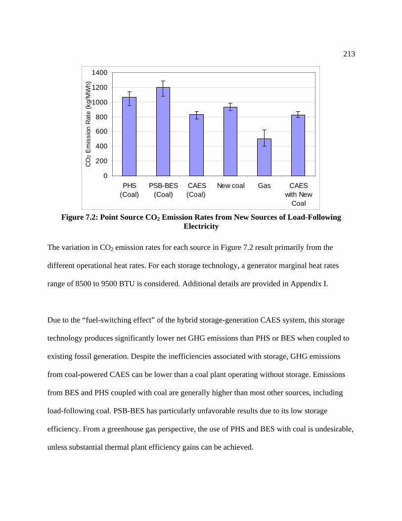
213

0

200

400

600

800

1000

1200

1400

PHS(Coal)

PSB-BES(Coal)

CAES(Coal)

New coal Gas CAESwith New

Coal

CO

2 E

mis

sion

Rat

e (k

g/M

Wh)

Figure 7.2: Point Source CO2 Emission Rates from New Sources of Load-Following

Electricity

The variation in CO2 emission rates for each source in Figure 7.2 result primarily from the

different operational heat rates. For each storage technology, a generator marginal heat rates

range of 8500 to 9500 BTU is considered. Additional details are provided in Appendix I.

Due to the “fuel-switching effect” of the hybrid storage-generation CAES system, this storage

technology produces significantly lower net GHG emissions than PHS or BES when coupled to

existing fossil generation. Despite the inefficiencies associated with storage, GHG emissions

from coal-powered CAES can be lower than a coal plant operating without storage. Emissions

from BES and PHS coupled with coal are generally higher than most other sources, including

load-following coal. PSB-BES has particularly unfavorable results due to its low storage

efficiency. From a greenhouse gas perspective, the use of PHS and BES with coal is undesirable,

unless substantial thermal plant efficiency gains can be achieved.

214Figures 7.3 and 7.4 provide SO2 and NOx emissions rates for the various load-following

sources.

0.0

4.0

8.0

12.0

16.0

20.0

PHS(Coal)

PSB-BES(Coal)

CAES(Coal)

New coal Gas CAESwith New

Coal

SO2

Emis

sion

Rat

e (k

g/M

Wh)

Figure 7.3: Point Source SO2 Emission Rates from New Sources of

Load-Following Electricity

0.0

1.0

2.0

3.0

4.0

5.0

6.0

7.0

PHS(Coal)

PSB-BES(Coal)

CAES(Coal)

New coal Gas CAES withNew Coal

NO

x Em

issi

on R

ate

(kg/

MW

h)

Figure 7.4: Point Source NOX Emission Rates from New Sources of

Load-Following Electricity

215The impacts of NSR are dramatic in terms of SOx and NOx emission rates. While there is a

large variation in emission rates for the storage systems coupled to older coal plants, their

emissions rates are typically much higher than any new source that could be legally constructed

for the generation of load-following or peaking power.

7.2.4 Analysis of the Emissions from a Proposed Energy Storage Facility – The Norton CAES Project As discussed previously, energy storage facilities are not required to consider their net emissions

under NSR, and therefore are not required to report these emissions when applying for pre-

construction permits. As a result, the public and regulators are left unaware of the actual impacts

on air quality that may result from the use of storage. This situation can be examined in detail by

estimating the annual emissions that will result from the operation of an actual proposed plant –

the Norton CAES facility.

As a major stationary source, the preconstruction permit application for the Norton CAES

facility was required to include an emissions and air quality analysis.46 This analysis, and the

other documents filed in support of the Norton CAES facility, provide no indication of the actual

emissions that will result from operation.47 In fact, there is very little mention of the fact that this

plant will be coupled primarily to power plants whose emissions greatly exceed NSPS. Section

7.2.3 demonstrates that even with the dramatically reduced marginal heat rate and the “fuel

switching effect” of coal-powered CAES, this new source of load-following and peaking power

will produce significantly higher levels of emissions than any other generation source that could

be legally constructed.

216Using the analysis in section 7.2.3, it is possible to estimate the emission rates and annual

emissions that will result from the operation of the Norton CAES facility. The net emissions

from this new source can then be compared to the emissions from alternatives that meet NSPS.

Alternatives include CAES coupled to a coal plant that meets NSPS, and two non-storage

alternatives: the combination of an intermediate load NSPS coal plant and a simple cycle gas

turbine, and the combination of combined cycle and simple cycle gas turbines.

According to the Norton CAES application, the completed plant will operate at a capacity factor

of 23-48%, with a maximum output of 2700 MW. The higher capacity factor is probably

optimistic, since PHS facilities in the U.S. seldom exceed 25% capacity factor, and are often

under 20%.48 This assessment assumes an annual capacity factor of 25%, producing annual

electric generation of 5913 GWh. Table 7.2 provides the total emissions that would result from

each of four systems that provide this amount of electricity. The two CAES/coal cases are based

on emission rates calculated in section 7.2.3, with the CAES ERnet reduced to 0.72, since the

CAES plant is located relatively close to load centers. The non-storage case with a NSPS coal

plant assumes an intermediate load coal plant with an average heat rate of 10,000 BTU,

producing 3000 GWh annually, and a simple-cycle gas turbine producing the remaining 2914

GWh at a heat rate of 10,500 BTU/kWh. The natural gas case assumes that 3000 GWh is

produced by a combined-cycle gas turbine operating at a heat rate of 8,500 BTU/kWh, with the

remainder produced by a single-cycle gas turbine.

217Table 7.2: Point Source Emissions from New Load-Following Electricity Generators Providing 5913 GWh Annually

Annual Fuel Consumption and Emissions for a 2700 MW Plant Operating at a 25% CF

Fuel Consumed (Billion BTU)

CO2 (tonnes) SO2 (tonnes) NOx (tonnes)

CAES with Typical Existing Coal Plant CAES Coal Total

24,834,600 36,613,296 61,447,896

1,806,153 3,411,693 5,217,846

7 22,967 22,974

339 8,321 8,660

CAES with Coal Plant Meeting NSPS CAES Coal Total

24,834,600 36,187,560 61,022,160

1,806,153 3,372,023 5,178,175

7 1,645 1,652

339 1,316 1,655

NSR Coal and GT Coal Gas Turbine Total

30,000,000 32,043,000 62,043,000

2,795,455 2,330,400 5,125,855

1,636

9 1,645

1,091 583

1,674 NSR Gas CCGT GT Total

25,500,000 32,043,000 57,543,000

1,854,545 2,330,400 4,184,945

7 9

16

348 583 930

CAES coupled to existing coal generation produces much higher levels of SO2 and NOx than

competing new sources of load-following power. The CAES plant will effectively produce at

least 13 times more SO2 and 5 times more NOx than the alternative plants that can legally be

constructed. These new sources must perform air modeling and conform to BACT standards.

The CAES plant must only consider the CAES turbines in its air modeling, and can completely

ignore the significant emissions that result from the coal combustion component of the CAES

facility.

Operating at a 25% capacity factor, the CAES plant coupled to an existing coal-fired plant will

annually “burn” in excess of 24 trillion BTU, roughly equivalent to the annual consumption of a

350 MW baseload coal power plant. In other words, the construction and use of the CAES

218facility in this manner is equivalent to constructing and operating a baseload 350 MW

coal-burning power plant without meeting any of the requirements of NSR.

While CAES coupled to pre-NSR plants produce high levels of SO2 and NOx, CAES coupled to a

new coal plant performs roughly equivalent to the new coal/gas combination, and would clearly

be superior to an all new coal scenario. In addition, the new coal/CAES system uses less natural

gas than the non-storage alternatives, so would be more fuel sustainable, have lower fuel costs,

and provide additional system benefits unique to energy storage.

This analysis demonstrates that for an accurate comparison of the emissions from CAES to an

alternative load following facility, emissions from the CAES electricity source should be

evaluated. Without such an analysis, there is tremendous bias towards the storage facility that is

potentially far more polluting than a new plant.

7.3 Policy Options for Addressing the Energy Storage Loophole

The analysis in section 7.2.3 demonstrates considerable emissions from the use of the Norton

CAES facility, or any facility coupled to an older coal generation facility. Any new conventional

source of electricity generation must meet NSR, which includes both providing an analysis of

emissions, and meeting certain emission standards. It is worth evaluating how an energy storage

system might meet the standards of NSR.

219

7.3.1 Accounting for Emissions from Energy Storage System An examination of the various application documents from the Norton CAES project and as the

TVA Regenesys project provides no indications of the air emissions that will result from storage

plant operations, beyond storage plant point source emissions. This omission limits the ability of

the public and policymaker to reasonably evaluate the emissions from different load-following

and peaking energy sources.

Application materials, testimony, and supporting information for the Norton Energy Storage

(NES) CAES facility give no indication of the fact that large amounts of emissions will result

from the use of CAES. During hearings on the proposed Norton CAES facility, testimony from a

NES official implies that off peak nuclear power may be used for the CAES compression cycle,

despite the clear lack of significant off-peak nuclear capacity. 49 In addition, the stated

“demonstrable environmental benefits associated with this CAES project” include “the use of

off-peak electric energy, and a [low] natural gas heat rate [that] combine to create a point source

emissions profile lower than any other available fossil-fired generation technology.”50

While this statement is technically correct, nowhere in the testimony or filings is any estimate of

total emissions that will result from CAES operation, even under hypothetical scenarios that

must have been generated for such a facility to be proposed as an IPP project.

220Another example of incomplete information regarding the actual emissions resulting from

energy storage is a statement in an article promoting CAES published by another CAES

developer, Ridge Energy Storage:

CAES is an environmentally friendly technology….Per-megawatt emissions from CAES are about one-third of conventional fossil fuel generation plants… The low thermal heat rate of a CAES plant (less than 4,500 Btu/kWh) enables it to produce power with about 60% fewer emissions than a comparably sized simple cycle plant or 30% fewer emissions than a similarly sized combined-cycle plant.51

This statement is demonstrably untrue, unless all compressor electricity is derived from nuclear

or renewable sources, which is highly unlikely for any of the proposed CAES facilities.

To provide the public and regulators with sufficient information to evaluate energy storage as a

source of load-following and peaking power, full accounting of emissions resulting from energy

storage should be required. Required documents, such as environmental impact statements,

should provide estimates of the emissions that will result from expected power purchases. Such

disclosures should, of course, estimate and report the substantial environmental benefits of

storage, including increased plant efficiency, reduced spinning reserve requirements, and any

other advantages unique to energy storage. Full accounting would be a first step in

acknowledging and addressing the energy storage loophole.

7.3.2 Closing the Energy Storage Loophole

If the energy storage loophole is to be considered significant enough to be specifically addressed,

there are two possible general remedies. If the net emissions from the use of energy storage are

221to meet NSPS, either the storage system operator or the electricity provider must be

responsible for ensuring that the standards are met. Each of these options can be examined

critically.

Option 1) Consider storage as a new source, whose effective emissions must meet NSPS One possible solution would be to require the storage plant to be responsible for its net

emissions. The storage plant would be responsible for tracking its net emissions by summing the

emissions that result from increased power plant output, and dividing this by its production rate.

To encourage the beneficial use of energy storage, the facility would be able to deduct offsets

that result from efficiency increases, as well as reduced emissions resulting from spinning

reserve provisions and other gains. To enable maximum economic efficiency, the emissions rate

would be measured as an average. Such a method would allow for flexible purchase agreements,

to meet a net output-based emissions standard.

Unfortunately, closing the loophole in this method would likely face significant opposition, and

has some significant practical limitations. Tracking emissions reductions due to efficiency

increases is difficult, and complicated by current input-based emissions standards. Measuring

energy storage emissions using an output-based standard would require a fundamental shift in

the manner in which emissions are monitored and recorded. Potentially more significant is the

amount of regulatory oversight that would be necessary to enforce provisions, and avoid

deceptive emissions accounting practices. As an example, the energy storage facility could

arrange to purchase power from a regulated utility that operates two power plants, a nuclear plant

which always runs at full capacity, and a grandfathered coal plant with spare off-peak capacity.

The operating utility could potentially increase the existing coal plant output (using the hours of

222operation exemption) to meet the baseload, which would free up the nuclear plant to sell its

“spare” capacity to the storage facility. Careful oversight would be necessary to monitor such

transactions. The significant technical and regulatory limitations of this approach makes this

solution unlikely. This solution also violates the basic “polluter pays” principle which is the

general standard for emissions responsibility. Any realistic solution will likely address emissions

at the source.

Option 2) Require the electricity sales to energy storage to meet NSR

Electricity sales to energy storage facilities could be required to meet NSR by altering the hours

of operation exemption. The EPA could promulgate a rule that limits the hours of operation

exemption in cases that consist of fundamental changes in method of operation. Long term,

planned, and utility-initiated increases in hours of operation that are accompanied by the use of

enabling technologies such as energy storage would fall outside the hours of operation

exemption. This rule would appear to be consistent with the language of the CAA. This solution

would also remove a market inconsistency for competing sources for new peaking power.

This solution is less complicated to administer, and is more transparent than the first option. It is

also more consistent with the general “polluter pays” principle, where the generator of emissions

is the responsible party for tracking and compliance. While this method does not account for the

potential emission reduction benefits of energy storage, it does not require any new accounting

methods that would be required with output-based standards.

223

7.4 Conclusions

Energy storage provides unique opportunities to electric power systems to increase the overall

flexibility of low emission sources such as nuclear and wind generation. However, in the near

term, the likely sources of electricity for energy storage are older coal-fired power plants with

high rates of emissions. The combination of energy storage and an older coal-fired plant creates a

new source of peaking power with emissions that typically greatly exceed the maximum

allowable emissions for a source that could be legally constructed. Since NSR allows for

increased output at older plants due to increased demand, NSR will not be triggered if a power

plant increases its output due to the use of energy storage. As a result, energy storage is a new

source of power that, while legal, appears to violate the intention of New Source Review. As

long as the hours of operation exemption remains in place, energy storage will be able to take

advantage of these older grandfathered plants, and energy storage will have an economic

advantage over sources of energy that produce lower amounts of environmentally harmful air

emissions.


1 40 C.F.R. Part 50. 2 42 U.S.C §7410. 3 42 U.S.C §7501-7515. 4 42 U.S.C §7470-7492. 5 42 U.S.C §7411. 6 42 U.S.C §7602(j). 7 42 U.S.C §7661.

224 8 40 C.F.R §52.21. 9 42 U.S.C §7475. 10 42 U.S.C §7501(3) and 7503(a)(2). 11 42 U.S.C §7501(a)(1)(A). 12 40 C.F.R §60.43(a). 13 42 U.S.C §7502(c). 14 H.R. Rept. 95-284, 145; 1977 CRS Legislative History, 2652. 15 National Academy of Public Administration. (April 2003) Breath of Fresh Air: Reviving the New Source Review Program Washington, D.C. 16 42 U.S.C §§7411(a)(4),7475(a),7479(2)(C),7501,7503 . 17 5 U.S.C §§551-559. 18 Chevron U.S.A., Inc. v. Natural Res. Def. Council, Inc., 467 U.S. 837, 104 S.Ct. 2778, 81

L.Ed.2d 694 (1984). 19 Id. at 862. 20 Id. at 865-866. 21 Id. at 865-66. 22 43 Federal Register 26830 (June 19, 1978). 23 Alabama Power v. Costle, 636 F.2d 323 (D.C. Cir. 1979) 636 F.2d at 358-361. 24 Id at 400. 25 40 C.F.R §60.14(e). 26 45 Fed Reg 52,676, 52,704 Aug 7, 1980. 27 Ayres, R.E. and R.W. Parker, (1992) The Proposed WEPCo Rule: Making the Problem Fit the

Solution. Environmental Law Reporter. 22(3): p. 10201-10210. 28 Wisconsin Electric Power Co. V. Reilly, 893 F.2d 901, (7th Cir. 1990).

225 29 U.S. Department of Justice, Office of Legal Policy. New Source Review: An Analysis of the

Consistency of Enforcement Actions with the Clean Air Act and Implementing Regulations. January 2002.

30 United States v. Ohio Edison Company, Case No. 2:99-CV-1181 (S.D. Ohio, August 2003). 31 Id. At 83. 32 Id. At 6. 33 United States v. Duke Energy Corp., 278 F.Supp.2d 619 (M.D.N.C. 2003). 34 67 Federal Register 80,205 (December 31, 2002). 35 Ibid. 36 68 Federal Register 61,248 (October 27, 2003). 37 State of New York v. United States Environmental Protection Agency, No. 03-1380 (D.C. Cir.

filed Oct. 27, 2003). 38 State and Territorial Air Pollution Program Administrators Viahttp://www.4cleanair.org/members/010204wklyupdateshell.pdf 39 Environmental Protection Agency (2004). E-Grid Database Via

http://www.epa.gov/cleanenergy/egrid/. 40 National Electric Reliability Council (2004) Generating Availability Data System Database

Via http://www.nerc.com/~gads/. 41 Black & Veatch., Power Plant Engineering. 1996: Chapman & Hall. 42 Environmental Protection Agency (2004). Proposed National Emission Standards for

Hazardous Air Pollutants; and, in the Alternative, Proposed Standards of Performance for New and Existing Stationary Sources:Electric Utility Steam Generating Units.

43 Intermountain Power Agency. (2003) Annual Report 2003. http://www.ipautah.com/pdf/IPA-

AnnaulReport-2003.pdf. 44 Wisconsin Public Service Corporation. (2003). Certificate of Public Convenience and

Necessity Application. Supercritical Pulverized Coal Electric Generating Facility Weston Unit 4 Project.

226 45 Termuehlen, H. and W. Emsperger (2003). Clean and Efficient Coal-Fired Power Plants. New

York, ASME Press. 46 Norton Energy Storage L.L.C. (2000). Application to the Ohio Power Siting Board for a

Certificate of Environmental Compatibility and Public Need (Summit County, Ohio). 47 Ohio Power Siting Board. (2001). In the Matter of the Application of Norton Energy Storage,

LLC for a Certificate of Environmental Compatibility and Public Need for an Electric Power Generating Facility In Norton, Ohio. Case 99-1626-EL-BGN (Summit County, Ohio).

48 Phillips, J., Pumped storage in a deregulated environment. International Journal on

Hydropower & Dams, 2000. 7(1): p. 32-35. 49 Ohio Power Siting Board. (2001) Testimony of Michael J. McGill. In the Matter of the

Application of Norton Energy Storage, LLC for a Certificate of Environmental Compatibility and Public Need for an Electric Power Generating Facility In Norton, Ohio Case 99-1626-EL-BGN (Summit County, Ohio).

50 Ibid. 51 Webb, R., (2001). An Electricity Savings Account. Energy Markets. 6(3).

227

8. Conclusions and Recommendations for Further Study

8.1 Conclusions

1) Intermittent electricity generation sources such as wind and solar energy impose burdens on

electric power systems that result in added costs. As the fraction of electrical energy provided by

intermittent increases, the delivered cost of this energy can increase dramatically. At some point,

energy storage becomes an economic necessity to allow an increase in the use of intermittent

sources. This amount is dependant on many factors, including renewable resource characteristics,

existing generation capabilities, and available energy storage technology. While much more

research is required to determine this economic break-even point, certainly 10-30% is reasonable

bound for the amount of wind energy that can be economically deployed in coal-based systems

where CAES geology is available.

2) The location of economic intermittent renewable resources such as wind will require a large

expansion of long distance transmission capacity. If intermittent wind energy is to provide a

large share (>20%) of the nation’s electrical energy supply, both transmission and energy storage

will need to be deployed on a large scale.

3) The number of storage technologies available for use with intermittent renewables is quite

small. Since pumped hydro is unlikely to be expanded due to environmental considerations and

geographic constraints, compressed air energy storage is the most likely technology for large-

scale storage of wind energy. Batteries may play an increased role for distributed energy systems

such as solar PV.

2284) In terms of environmental impact, energy storage systems are mostly “pass through”

technologies. The “life-cycle” components of energy storage systems, such as construction and

O&M are a relatively small fraction of net environmental impact for most technologies. Only the

fuel delivery component of CAES produces a large amount of energy use and emissions,

especially compared to emissions and energy use from fossil energy production.

5) Since the energy use and CO2 emissions from energy storage systems are largely a function of

the primary generation source, the lowest efficiency technologies such as PSB-BES will result in

the greatest energy use and emissions, particularly when coupled to highly polluting sources. The

net GHG emission rate from PSB-BES is about 15% higher than the VRB-BES or PHS. The

unique hybrid-CAES system has lower GHG emissions than any other storage technologies

when coupled to fossil source. When coupled to coal, GHG emissions from CAES are at least

25% lower than any other storage technology.

6) Considering both transmission and distribution provides additional insights into the actual

environmental impact of electricity generation technologies. While the impact of T&D

construction and O&M is relatively small, T&D losses can significantly increase the impact from

fossil sources. This issue is of particular concern when considering large-scale development of

the nations extensive lignite resources in the upper Midwest. Emissions related only to the T&D

of lignite derived electricity will typically exceed 100 kg/MWh.

7) Integrated renewable/storage/transmission systems can be an alternative to conventional

generation systems. Wind/CAES can be deployed on a large scale, and demonstrates high levels

229of fossil energy sustainability, delivering more 5 times the amount of electrical energy from a

unit of fossil fuel than the most efficient combustion system available. The GHG emissions from

a wind/CAES system are about 20% of the lowest emission fossil system in existence. Both

wind/PHS and Solar PV/BES also demonstrate superior performance to fossil energy systems in

terms of energy sustainability and GHG emissions for intermediate and peaking generation.

8) Since the environmental impact of energy storage systems reflect the primary generation

source, their use is not necessarily positive in terms of air emissions. The unique

“grandfathering” provisions of the U.S. clean air act allow for increased output from existing

coal plants that produce high levels of emissions. Energy storage provides a loophole that could

be used to increase output from these plants, instead of building cleaner alternatives. A proposed

CAES plant that has been permitted will effectively produce SO2 at a rate more than 10 times the

amount allowed by law for a new power plant. Its effective NOx emission rate could be as high

as 5 times greater than legally permitted for a new plant. This loophole has been largely

overlooked, and should be examined critically if new technologies for generation of peaking and

load-following power are to be compared equally to the use of energy storage with existing coal

fired power plants.

8.2 Recommendations for Further Study

1) Significant work remains in understanding the economic limits of intermittent sources in

existing electric power networks. Potentially the most significant benefits would be a better

quantification of the incremental cost of wind energy integration at higher capacity and energy

penetration. Furthermore, this quantification should be able to account for the changing nature of

230the electric power grid, including the use of different generation technologies, but also

considering the effects of deregulation.

2) A more advanced model of national wind energy penetration should be developed. This has

significant policy implications. If wind energy is only able to provide a fairly small percentage of

the U.S. electric demand without significant transmission developments, long-term transmission

planning policies in the U.S. must be developed appropriately. The interaction between wind

energy and future low-carbon sources should also be examined. The use of large amounts of

wind energy in a system without the use of storage is dependent on overall system flexibility.

Two possible low-carbon power sources, nuclear energy and integrated gasification combined-

cycle (IGCC) with carbon capture are far less flexible than current gas and coal generation

technologies. In a sense, nuclear energy and wind are, to a certain extent, mutually exclusive

technologies. It is conceivable that large scale deployment of wind energy could limit the use of

these technologies (or the opposite may alternatively be true.)

3) The metrics of energy analysis and environmental impact related to electric power systems

can be improved with additional research. As suggested in Chapter 3, energy discounting would

provide more meaningful results in terms of net energy production. Discounting of carbon

emissions would provide a better assessment of GHG emission rates. In additional, appropriate

“weighting” of energy sources should be addressed.

2314) The large scale use of intermittent renewables will require new metrics for understanding

their social and environmental impacts. Significant areas of research must consider relative land

use, aesthetics, and risk perception.

The large scale deployment of renewable energy systems will require the construction of new

technologies that will have a fundamentally different set of visual impacts and perceived risks

compared to existing technologies. New development is potentially challenged by increased

concerns regarding the environmental impacts of electric power systems, concerns that did not

exist when much of the existing electric power infrastructure was developed. Much work

remains to understand the social acceptability of large scale renewable energy systems.

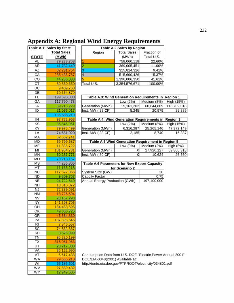
232

Appendix A: Regional Wind Energy Requirements Table A.1: Sales by State

STATETotal Sales

(MWh)Region Total Sales

(MWh)Fraction of Total U.S.

AL 79,233,768 1 758,060,118 22.60%AR 41,732,449 2 369,005,451 11.00%AZ 62,281,754 3 315,814,326 9.41%CA 235,438,767 4 515,690,426 15.37%CO 44,236,038 5 1,396,006,350 41.61%CT 30,530,550 Total U.S. 3,354,576,671 100.00%DC 9,409,760DE 10,664,879FL 199,698,300GA 117,790,473 Low (2%) Medium (8%) High (15%)IA 39,213,229 Generation (MWh) 15,161,202 60,644,809 113,709,018ID 21,096,017 Inst. MW (.33 CF) 5,245 20,979 39,335IL 135,685,219IN 97,733,968KS 35,846,951 Low (2%) Medium (8%) High (15%)KY 79,975,499 Generation (MWh) 6,316,287 25,265,146 47,372,149LA 74,681,020 Inst. MW (.33 CF) 2,185 8,740 16,387MA 52,662,741MD 59,799,687ME 11,835,722 Low (0%) Medium (2%) High (5%)MI 101,954,781 Generation (MWh) 0 27,920,127 69,800,318MN 60,287,771 Inst. MW (.30 CF) 0 10,624 26,560MO 73,213,157MS 44,286,865MT 11,165,218NC 117,622,866 30ND 9,809,757 0.75NE 24,722,640 197,100,000NH 10,316,372NJ 72,339,691NM 18,726,594NV 28,167,293NY 141,398,705OH 154,458,595OK 49,666,725OR 45,884,830PA 137,893,545RI 7,846,557SC 74,832,367SD 8,626,999TN 95,320,199TX 316,061,963UT 23,217,308VA 96,122,996VT 5,617,438 Consumption Data from U.S. DOE "Electric Power Annual 2001" WA 79,666,210 DOE/EIA-0348(2001) Available at:WI 65,183,501 http://tonto.eia.doe.gov/FTPROOT/electricity/034801.pdfWV 27,669,432WY 12,949,505

Table A.6 Parameters for New Export Capacity for Scenario 2

System Size (GW)Capcity FactorAnnual Energy Production (GWh)

Table A.3: Wind Generation Requirements in Region 1

Table A.5 Wind Generation Requirement in Region 5

Table A.2 Sales by Region

Table A.4: Wind Generation Requirements in Region 3

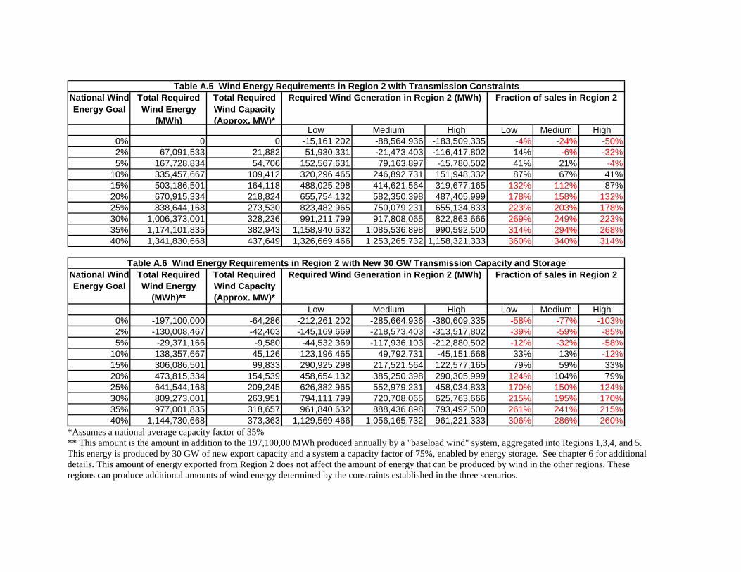
National Wind Energy Goal

Total Required Wind Energy

(MWh)

Total Required Wind Capacity (Approx. MW)*

Low Medium High Low Medium High0% 0 0 -15,161,202 -88,564,936 -183,509,335 -4% -24% -50%2% 67,091,533 21,882 51,930,331 -21,473,403 -116,417,802 14% -6% -32%5% 167,728,834 54,706 152,567,631 79,163,897 -15,780,502 41% 21% -4%

10% 335,457,667 109,412 320,296,465 246,892,731 151,948,332 87% 67% 41%15% 503,186,501 164,118 488,025,298 414,621,564 319,677,165 132% 112% 87%20% 670,915,334 218,824 655,754,132 582,350,398 487,405,999 178% 158% 132%25% 838,644,168 273,530 823,482,965 750,079,231 655,134,833 223% 203% 178%30% 1,006,373,001 328,236 991,211,799 917,808,065 822,863,666 269% 249% 223%35% 1,174,101,835 382,943 1,158,940,632 1,085,536,898 990,592,500 314% 294% 268%40% 1,341,830,668 437,649 1,326,669,466 1,253,265,732 1,158,321,333 360% 340% 314%

National Wind Energy Goal

Total Required Wind Energy

(MWh)**

Total Required Wind Capacity (Approx. MW)*

Low Medium High Low Medium High0% -197,100,000 -64,286 -212,261,202 -285,664,936 -380,609,335 -58% -77% -103%2% -130,008,467 -42,403 -145,169,669 -218,573,403 -313,517,802 -39% -59% -85%5% -29,371,166 -9,580 -44,532,369 -117,936,103 -212,880,502 -12% -32% -58%

10% 138,357,667 45,126 123,196,465 49,792,731 -45,151,668 33% 13% -12%15% 306,086,501 99,833 290,925,298 217,521,564 122,577,165 79% 59% 33%20% 473,815,334 154,539 458,654,132 385,250,398 290,305,999 124% 104% 79%25% 641,544,168 209,245 626,382,965 552,979,231 458,034,833 170% 150% 124%30% 809,273,001 263,951 794,111,799 720,708,065 625,763,666 215% 195% 170%35% 977,001,835 318,657 961,840,632 888,436,898 793,492,500 261% 241% 215%40% 1,144,730,668 373,363 1,129,569,466 1,056,165,732 961,221,333 306% 286% 260%

Table A.5 Wind Energy Requirements in Region 2 with Transmission ConstraintsRequired Wind Generation in Region 2 (MWh) Fraction of sales in Region 2

Required Wind Generation in Region 2 (MWh) Fraction of sales in Region 2Table A.6 Wind Energy Requirements in Region 2 with New 30 GW Transmission Capacity and Storage

*Assumes a national average capacity factor of 35% ** This amount is the amount in addition to the 197,100,00 MWh produced annually by a "baseload wind" system, aggregated into Regions 1,3,4, and 5. This energy is produced by 30 GW of new export capacity and a system a capacity factor of 75%, enabled by energy storage. See chapter 6 for additional details. This amount of energy exported from Region 2 does not affect the amount of energy that can be produced by wind in the other regions. These regions can produce additional amounts of wind energy determined by the constraints established in the three scenarios.

234

Mt. Elbert CO 1981 200 12 2410 a,Racoon Mtn. TN 1978 1530 21 31400 a,Rocky Mtn. GA 1995 760 8 6080 a,h,I

Table B.1: Basic Data Related to PHS Systems Analyzed

Appendix B: Pumped Hydro Storage Data

Project Name Location First Power Date

Power (MW)

Storage Time

(hours)

Storage Energy (MWh)

References

Bad Creek SC 1991 1000 24 24000 a,bBalsam Meadow CA 1987 200 8 1600 a,Bath County VA 1985 2100 11 23700 a,c,d,eClarence Cannon MO 1984 31 9 265 a,Fairfield SC 1978 512 8 4096 a,Helms CA 1984 1206 15* 18090 a,f,g

*Storage time for Helms based on weighted average on remaining plants due to inconsistencies in reported data. All Data for the Basic Data, Dams, Underground Components, Power House, Excavation, and Land Use is derived from the following references: a) Task Committee on Pumped Storage of the Hydropower Committee of the Energy Division of the American Society of Civil Engineers. (1993.) Compendium of Pumped Storage Plants in the United States, American Society of Civil Engineers, New York. b) McLaren, D. G., et al. (1989). Design features of the Bad Creek pumped storage project generators motors. IEEE Transactions on Energy Conversion 4(2): pp. 191-6. c) Anon. (1985). Bath county pumped storage. Civil Engineering (American Society of Civil Engineers) 55: pp. 55. d) Danilevsky, A. (1984). Superhydro: Virginia's Bath County Pumped Storage Project. Civil Engineering 54: pp. p. 54-7. e) Zagars, A. and J. M. Hagood (1977). Bath County, a 2100 MW Development in the USA. International Water Power and Dam Construction Oct. f) Anon. (1985). Helms pumped storage project. Civil Engineering (American Society of Civil Engineers) 55: pp. 50 g) Paul, K. (1989). Design features of the Helms pumped storage project. IEEE Transactions on Energy Conversion 4(1): pp. 9-14. h) Konstantellos, C., et al. (1997). Rocky Mountain Pumped-Storage Project in Operation since the Summer of 1995. Waterpower '97 i) Murphy, D. R. and W. R. Ivarson (1991). Rocky Mountain Project Will Provide Peak Power for Georgia. International Water Power and Dam Construction Feb.: pp. 22-24.

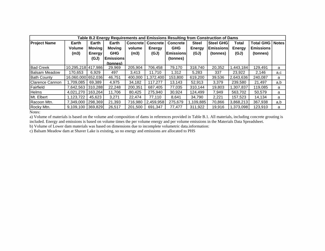
Project Name Earth Volume

(m3)

Earth Moving Energy

(GJ)

Earth Moving

GHG Emissions (tonnes)

Concrete volume

(m3)

Concrete Energy

(GJ)

Concrete GHG

Emissions (tonnes)

Steel Energy

(GJ)

Steel GHG Emissions (tonnes)

Total Energy

(GJ)

Total GHG Emissions (tonnes)

Notes

Bad Creek 10,295,218 417,986 29,969 205,904 706,458 79,170 318,740 20,352 1,443,184 129,491 aBalsam Meadow 170,653 6,929 497 3,413 11,710 1,312 5,283 337 23,922 2,146 a,cBath County 16,060,000 652,036 46,751 400,000 1,372,400 153,800 619,200 39,536 2,643,636 240,087 aClarence Cannon 1,709,085 69,389 4,975 34,182 117,277 13,143 52,913 3,379 239,580 21,497 a,bFairfield 7,642,563 310,288 22,248 200,351 687,405 77,035 310,144 19,803 1,307,837 119,085 aHelms 4,021,270 163,264 11,706 80,425 275,940 30,924 124,499 7,949 563,702 50,579 aMt. Elbert 1,123,722 45,623 3,271 22,474 77,110 8,641 34,790 2,221 157,523 14,134 aRacoon Mtn. 7,349,000 298,369 21,393 716,980 2,459,958 275,679 1,109,885 70,866 3,868,213 367,938 a,bRocky Mtn. 9,109,100 369,829 26,517 201,500 691,347 77,477 311,922 19,916 1,373,098 123,910 a

Table B.2 Energy Requirements and Emissions Resulting from Construction of Dams

Notes: a) Volume of materials is based on the volume and composition of dams in references provided in Table B.1. All materials, including concrete grouting is included. Energy and emissions is based on volume times the per volume energy and per volume emissions in the Materials Data Spreadsheet. b) Volume of Lower dam materials was based on dimensions due to incomplete volumetric data.information: c) Balsam Meadow dam at Shaver Lake is existing, so no energy and emissions are allocated to PHS

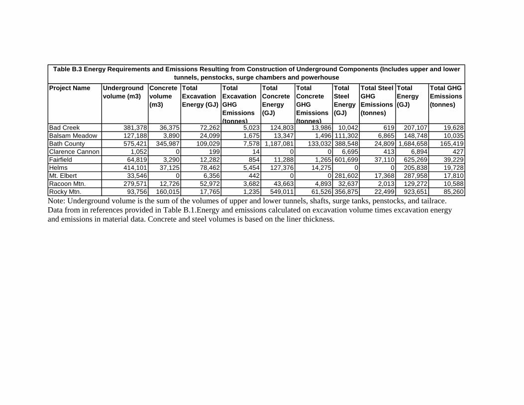
Project Name Underground volume (m3)

Concrete volume (m3)

Total Excavation Energy (GJ)

Total Excavation GHG Emissions (tonnes)

Total Concrete Energy (GJ)

Total Concrete GHG Emissions (tonnes)

Total Steel Energy (GJ)

Total Steel GHG Emissions (tonnes)

Total Energy (GJ)

Total GHG Emissions (tonnes)

Bad Creek 381,378 36,375 72,262 5,023 124,803 13,986 10,042 619 207,107 19,628Balsam Meadow 127,188 3,890 24,099 1,675 13,347 1,496 111,302 6,865 148,748 10,035Bath County 575,421 345,987 109,029 7,578 1,187,081 133,032 388,548 24,809 1,684,658 165,419Clarence Cannon 1,052 0 199 14 0 0 6,695 413 6,894 427Fairfield 64,819 3,290 12,282 854 11,288 1,265 601,699 37,110 625,269 39,229Helms 414,101 37,125 78,462 5,454 127,376 14,275 0 0 205,838 19,728Mt. Elbert 33,546 0 6,356 442 0 0 281,602 17,368 287,958 17,810Racoon Mtn. 279,571 12,726 52,972 3,682 43,663 4,893 32,637 2,013 129,272 10,588Rocky Mtn. 93,756 160,015 17,765 1,235 549,011 61,526 356,875 22,499 923,651 85,260

Table B.3 Energy Requirements and Emissions Resulting from Construction of Underground Components (Includes upper and lower tunnels, penstocks, surge chambers and powerhouse

Note: Underground volume is the sum of the volumes of upper and lower tunnels, shafts, surge tanks, penstocks, and tailrace. Data from in references provided in Table B.1.Energy and emissions calculated on excavation volume times excavation energy and emissions in material data. Concrete and steel volumes is based on the liner thickness.

237

Project Name Total Underground Excavation in Table B.3 m3

Total Fill Required m3

Total Excavation Required to

provide Fill (m3)

Additional Fill

Required (m3)

Energy For Additional

Fill (GJ)

GHG Emissions For Additional Fill

(tonnes)

Bad Creek 381,378 10,295,218 2,573,805 2,192,427 251,766 17,548Balsam Meadow 118,716 170,653 42,663 -76,053 -8,733 -609Bath County 575,421 16,060,000 4,015,000 3,439,579 394,982 27,530Clarence Cannon 1,052 1,709,085 427,271 426,219 48,945 3,411Fairfield 64,819 7,642,563 1,910,641 1,845,822 211,964 14,774Helms 414,101 4,021,270 1,005,318 591,217 67,892 4,732Mt. Elbert 33,546 1,123,722 280,931 247,385 28,408 1,980Racoon Mtn. 266,067 7,349,000 1,837,250 1,571,183 180,426 12,576Rocky Mtn. 93,756 9,109,100 2,277,275 2,183,519 250,743 17,477

Table B.4 Energy Requirements and Emissions Resulting from Excavation

This table calculates the energy required to quarry rock fill for dams. Much of the material is derived from required underground excavation. This chart calculates additional fill materials to be quarried. Assumes all fill materials require 25% rock composition. Any material not derived from tunneling is quarried on site and requires normal fill moving operation.

Project Name

Total Land Area Cleared or Flooded (m2)

Total Land Intensity M2/MWh Total energy Emissions Notes

Bad Creek 1,490,000 62 1,323 46,047Balsam Meadow 240,000 150 213 7,417Bath County 3,310,000 140 2,939 102,292 cClarence Cannon 48,862

807,0101,900,886

2,411,571

184 43 1,510Fairfield 197 717 24,940Helms 105 1,688 58,745Mt. Elbert 1,140,000 473 1,012 35,230 bRacoon Mtn. 77 2,141 74,527Rocky Mtn. 4,505,000 741 4,000 139,222 a

Table B.5 Energy Requirements and Emissions Resulting from Land Clearing and Biomass Removal

Notes a. Rocky mountain auxillary pools "primarily for recreation" but also provide make-up water, allocated 50% to PHS b. Lower reservoir partially existing, so only upper area used. c. Balsam Meadow dam at Shaver Lake is existing, so no energy and emissions are allocated to PHS

238

Item Typical Cost (1997 $/kW)

EIO Energy Factor (MJ/ 1997 $)

EIO Emissions Factor (grams/ 1997 $)

Energy Factor (GJ/MW)

Emissions Factor (kg/MW)

Turbine/Generator 195 7.19 520.39 1,403 101,476Other Electrical 40.5 8.00 575.00 324 23,288Misc Equipment 15 5.911613 429.987506 89 6,450Other Civil Works 45 9.93 844.36 447 37,996Total NA NA NA 2,262 169,210

Table B.6 Calculation of Energy and Emissions Related to Electrical System and Balance of Plant

The cost of each component was based on the weighted average costs (based on power) of components at Bad Creek, Bath County, Helms, and Rocky Mountain, derived from FERC Form 1 financial data. All EIO factors derived from Green Design Initiative. (2001) EIOLCA.net - Economic Input-Output Life Cycle Assessment. Carnegie Mellon University. Via http://www.eiolca.net. Accessed November 24, 2001.

Table B.7 Energy Requirements and Emissions Related to PHS Electrical System and Balance of Plant

Project Name Power (MW) Energy (GJ) GHG Emissions (tonnes)

Bad Creek 1000 2,262,306 169,210Balsam Meadow 200 452,461 33,842Bath County 2100 4,750,843 355,340Clarence Cannon 31 70,131 5,245Fairfield 512 1,158,301 86,635Helms 1206 2,728,341 204,067Mt. Elbert 200 452,461 33,842Raccoon Mtn. 1530 3,461,329 258,891Rocky Mtn. 760 1,719,353 128,599 Energy and emission factors in Table B.6 were multiplied by the size of each facility.

239

Project Name Cost (k$) Total Energy

(GJ)

GHG Emissions (tonnes)

Bad Creek 9,078 44,409 3,273Balsam Meadow 1,579 7,723 569Bath County 53,017 259,354 19,114Clarence Cannon 245 1,197 88Fairfield 4,041 19,770 1,457Helms 9,520 46,569 3,432Mt. Elbert 1,579 7,723 569Racoon Mtn. 12,077 59,079 4,354Rocky Mtn. 5,999 29,347 2,163

Table B.8 Energy Requirements and Emissions Resulting from Decommisioning

Decommissioning costs estimated at 10% of capital equipment costs. Frank R. Walker Company, (1999) The Building Estimator's Reference Book (26th ed.) Chicago, IL. EIO factor for general construction derived from Green Design Initiative. (2001) EIOLCA.net - Economic Input-Output Life Cycle Assessment. Carnegie Mellon University. Via http://www.eiolca.net. Accessed November 24, 2001.

Table B.9 Total Energy Requirements and Emissions Resulting from the Construction of PHS Systems Project Name Total

Construction Energy (GJ)

Total Construction GHG Emissions (tonnes)

EES (GJ/MWh storage time)

EMS (tonnes CO2e/MWh storage time)

Life-Cycle Energy Rate (GJ/MWh)

Life Cycle Emissions Rate (kg CO2e/MWh)

Weighted EES

Weighted EMS

Bad Creek 4,210,095 385,197 175 16 40 4 175,421 16,050 Balsam Meadow 624,333 53,401 390 33 30 3 78,042 6,675 Bath County 9,736,412 909,782 411 38 44 4 862,720 80,614 Clarence Cannon 366,790 32,178 1,384 121 113 10 42,908 3,764 Fairfield 3,323,858 286,120 811 70 62 5 415,482 35,765 Helms 3,614,030 341,282 200 19 29 3 240,935 22,752 Mt. Elbert 935,086 103,565 388 43 44 5 77,601 8,595 Raccoon Mtn. 7,700,460 728,873 245 23 48 5 375,214 35,515 Rocky Mtn. 4,300,192 496,630 707 82 54 6 537,524 62,079 Weighted Average Results: EES = 372 GJ/MWh Storage Time EMS = 36 tonnes CO2e/MWh Storage Time

240

Appendix C: Compressed Air Energy Storage Data

Table C.1 Results: Energy Requirements and GHG Emissions from Operation Component Electrical

Energy Input (kWhin/kWhout)

Thermal Energy Input (kJ/kWhout)

GHG EmissionRate (kg CO2e/MWh)

Source Table

Primary Electricity 0.735 C.3 Delivered Natural Gas Fuel 4,649.40 233.96 C.3 Natural Gas Delivery 518.01 52.01 C.7 Other Variable (O&M + SCR) 27.08 2.00 C.7 Total Plant (without gas infrastructure) 26.31 1.98 C.4 & C.5 Natural Gas Infrastructure 29.78 2.11 C.4 Total 0.735 5,251 292

241Table C.2 Summary of CAES System Performance Specifications

Item Value Units Ref Notes CAES Heat Rate 4536 kJ/kWh 1pg5 A Net Heat Rate 4649.4 kJ/kWh B CAES Energy Ratio 0.7 kWhin/kWhout 1pg5 Storage Loss Factor 1 None No cavern losses (see text) Transmission Loss Factor 1.025 None 2.5% each way (see text) Net Energy Ratio 0.735 kWhin/kWhout C Natural Gas Capacity Req. 3402 MJ/sec D Maximum Power Output 2700 MW 1pg5 Storage Capacity 43200 MWh 1 Minimum CF 0.23 None 1pg19 This assesment does Maximum CF 0.48 None 1pg19 not use these CFS Annual Plant Output (min) 5,439,960 MWh Annual Plant Output (max) 11,352,960 MWh Annual O&M Cost (min) 20 $Million 1 pg 62 Annual O&M Cost (max) 30 $Million 1 pg 62 Assumed Plant Lifetime 40 Years Assumed Annual Plant Output 4,730,400 MWh Assumes .20 CF Assumed Total Plant Output 189,216 GWh Natural Gas Emission Factor 0.0503 tonnes co2e/gj 2 Point Source GHG Emissions 233.96 kg CO2e/MWh References 1. Norton Energy Storage L.L.C. (2000). Application to the Ohio Power Siting Board for a Certificate of Environmental Compatibility and Public Need. Summit County, Ohio. 2. Spath, P. L. and M. K. Mann (2000). Life Cycle Assessment of a Natural Gas Combined-Cycle Power Generation System. National Renewable Energy Laboratory. Golden, CO. NREL/TP-570-27715. Notes: A) The quoted heat rate of 3884 btu/kwh uses a lower heating value (LHV) of natural gas. This is equivalent to 4303.4 BTU/kWh using the higher heating value (HHV) which has a ratio 1.108 (22985 btu/lb hhv and 20745 btu/lb lhv from ref 2 which is equivalent to 4535.6 kJ/kWh B) Equals heat rate times output transmission loss factor C) Equals ER * output TL factor * input TL factor (both of which are = in this calculation) D) Equals power*heat rate (NOT net heat rate)

242

Table C.3: Plant Construction and Decommissioning (gas plant components)

Component Std. Plant Energy (GJ)

Std Plant Emissions (tonnes CO2e)

CAES adjustment Factor (multiplier)

CAES ConstructionEnergy (GJ)

CAES Construction Emissions (tonnes CO2e)

Combustion Turbines 570,073 41,273.21 1.70 968,205 70,098Recuperator (Roughly equiv. to CCGT HRSG) 35,187 2,566.00 1.70 59,761 4,358Transformers 65,158 4,725.48 4.35 283,751 20,579Pumps 38,067 2,714.79 1.00 38,067 2,715Electrical Equipment 83,048 5,893.54 4.35 361,659 25,665Noise Attenuation 1,780 125.94 1.00 1,780 126Road upgrades 4,638 300.54 1.00 4,638 301Pipeline & Header Interconnect 42,064 2,926.06 4.35 183,182 12,743construction 695,305 48,582.08 1.70 1,180,898 82,511building materials 125,891 20,736.95 1.70 213,811 35,219Decommissioning 59,221 3,959.72 1.70 100,581 6,725Natural Gas Infrastructure 2,140,248 151,426.82 2.70 5,777,924 408,800

Scaling Factors: Proportional 4.35 Turbines 1.70 Gas Infrastructure 2.70 Notes on Calculations: Since there are many common components between a CAES plant, and a gas turbine plant, the results for each CAES component was calculated by scaling the results from a previous study of a gas-turbine power plant. The previous study was an evaluation of a 620 MW combined cycle plant. This study is a 2700MW CAES plant. Each component was scaled based on the relative size. Four scaling factors were used: Scaling factor = 1 for the few components that would be nearly identical in both cases. Scaling factor = 2700/630 or 4.35 was used for certain power components, such as electrical equipment that are directly proportional to plant size. Scaling factor = 1.7 was used for several other components. This scaling factor is a result of the effective power output of a CAES turbine, which is equal to about 300/117 that of a conventional gas turbine (see text) So this scaling factor is actually 2700/630 times 117/300. Scaling factor = 2.7 was used for the natural gas infrastructure required by CAES. This factor is a the result of upscaling the natural gas fuel consumption rate for the gas plant (equal to the product of capcity and heat rate) to the CAES consumption rate. This is equal to 2700/630 times (4649*7500) where 7500 is the heat rate of the gas plant. Source of gas turbine data: Meier, P. J. (2002). Life-Cycle Assessment of Electricity Generation Systems and Applications for Climate Change Policy Analysis, Ph.D. Dissertation, University of Wisconsin - Madison.

243

Table C.4 Plant Construction and Decommissioning (CAES specific components)

Component Cost (M$)

cpi adj Total CAES Cost in 1997M$

EIO Factor (GJ/M$ 1997)

EIO Factor (tonnes CO2e/ M$ 1997)

Total Energy (GJ)

Total Emissions (tonnes CO2e)

Notes

Compressors/related 76.50 1.2 93.57 6,301.35 454.41 589,648 42,521A Cavern Development 94.35 1.2 115.40 3,858.36 277.25 445,267 31,996B Additional T&D 45.00 1.0 45.00 9,000.84 642.79 405,038 28,926C Notes: A: Cost derived from EPRI (1994), scaled to reflect a total of 9 compressors. EIO Factor is for "Pumps and Compressors" at EIOLCA.net B: Cost derived from EPRI (1994), scaled to reflect total cavern size of 43200 MWh. EIO Factor is for "Well Drilling" at EIOLCA.net C: Cost derived from NES (2002). EIO Factor is for were derived from the Green Design Initiative at EIOLCA.net References: Electric Power Research Institute. (1994). Standard compressed-air energy storage plant: design andcost. EPRI. Palo Alto, Calif. TR-103209. Norton Energy Storage L.L.C. (2000). Application to the Ohio Power Siting Board for a Certificate ofEnvironmental Compatibility and Public Need. Summit County, Ohio. EIOLCA.net is the Economic Input/Output LCA Database maintained by the Green Design Initiative. Website at www.eiolca.net. All data is from the 1997 data set.

Table C.5 Total Energy Input and Emissions for Construction (EES and EMS) Total CAES Const.

Energy (GJ) Total CAES

Const. Emissions

(tonnes CO2e)

EES (GJt/MWh Storage Capacity)

EMS (tonnes CO2e/MWh Storage

Capacity)

10,614,209 773,282 246 18 These are the totals of all fixed components from tables C.3 and C.4. The EES and EMS values are the totals divided by the CAES storage capacity (43200 MWh)

244

Table C.6 Operation and Maintenance, and Fuel Delivery Natural Gas Delivery

Energy Requirements (GJt/GJ gas delivered)

Emissions (tonnes CO2e/GJ Gas Delivered)

Energy (GJt/GWh)

Emissions (kg CO2e/MWh)

Notes/ Source

0.1114 0.0112 518.01 52.01A Non Fuel O&M Cost ($/MWh)Energy

Intensity of Maint (GJ/$)

co2 Intensity of Maint (tonnes/GJ)

Energy (GJt/GWh)


Notes/ Source

5.5 0.0049 362.8 27.08 2.00B SCR Gas Plant

Heat Rate (GJ/GWHe)

Gas Plant SCR Energy Rate (GJ/GWHe)

Gas Plant SCR Emission Rate (kg CO2e/MWh)

Energy (GJt/GWh)


Notes/ Source

7378 8.5 0.44 5.23 0.28C Notes: A: Natural Gas energy requirement is based on Meier (2002) where 136,151,287 GJ of Gas is required to deliver 1,222,020,000 GJ of Gas. Emissions to deliver this amount of gas is equal to 13,671,272 tonnes CO2e. These energy and emissions factor were then scaled to the CAES heat rate B: O&M cost data from Table C.3. EIO factor is for "Other Repair and Maintenance Construction" at EIOLCA.net. C: SCR data derived from Spath and Mann (2000) These values scaled to CAES plant heat rate. Refs: Meier, P. J. (2002). Life-Cycle Assessment of Electricity Generation Systems and Applications for Climate Change Policy Analysis, Ph.D. Dissertation, University of Wisconsin - Madison. Spath, P. L. and M. K. Mann (2000). Life Cycle Assessment of a Natural Gas Combined-Cycle Power Generation System. National Renewable Energy Laboratory. Golden, CO. NREL/TP-570-27715.

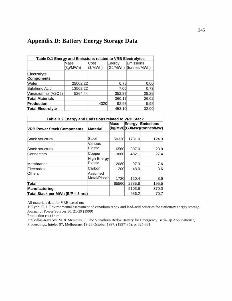
245

Appendix D: Battery Energy Storage Data

Table D.1 Energy and Emissions related to VRB Electrolytes

Mass (kg/MWh)

Cost ($/MWh)

Energy (GJ/MWh)

Emissions (tonnes/MWh)

Electrolyte Components Water 25002.22 0.75 0.00Sulphuric Acid 13562.22 7.05 0.73Vanadium as (V2O5) 5264.44 352.37 25.29Total Materials 360.17 26.02Production 4320 92.93 5.98Total Electrolyte 453.10 32.00

Table D.2 Energy and Emissions related to VRB Stack

VRB Power Stack Components Material Mass (kg/MW)

Energy (GJ/MW)

Emissions (tonnes/MW)

Stack structural Steel 50320 1731.0 124.3

Stack structural Various Plastic 6560 307.0 23.9

Connectors Copper 3680 482.1 27.4

Membranes High Energy Plastic 2080 97.3 7.6

Electrodes Carbon 1200 48.0 3.6Others Assumed

Metal/Plastic 1720 120.4 8.6Total 65560 2785.8 195.5Manufacturing 5103.6 370.0Total Stack per MWh (E/P = 8 hrs) 986.2 70.7 All materials data for VRB based on: 1: Rydh, C. J. Environmental assessment of vanadium redox and lead-acid batteries for stationary energy storage. Journal of Power Sources 80, 21-29 (1999) Production cost from: 2: Skyllas-Kazacos, M. & Menictas, C. The Vanadium Redox Battery for Emergency Back-Up Applications", Proceedings, Intelec 97, Melbourne, 19-23 October 1997. (1997).(5): p. 825-831.

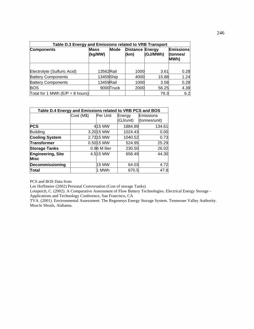
246

Table D.3 Energy and Emissions related to VRB Transport Components Mass

(kg/MW) Mode Distance

(km) Energy (GJ/MWh)

Emissions (tonnes/ MWh)

Electrolyte (Sulfuric Acid) 13562Rail 1000 3.61 0.28 Battery Components 13459Ship 4000 15.88 1.24 Battery Components 13459Rail 1000 3.58 0.28 BOS 9000Truck 2000 56.25 4.39 Total for 1 MWh (E/P = 8 hours) 79.3 6.2

Table D.4 Energy and Emissions related to VRB PCS and BOS Cost (M$) Per Unit Energy

(GJ/unit) Emissions (tonnes/unit)

PCS 4 15 MW 1884.89 134.61Building 3.20 15 MW 1024.43 0.00Cooling System 2.73 15 MW 1040.52 0.73Transformer 0.50 15 MW 524.95 25.29Storage Tanks 0.9 6 M liter 230.50 26.02Engineering, Site Misc

4.5 15 MW 658.49 44.30

Decommissioning 15 MW 64.03 4.72Total 1 MWh 670.5 47.8 PCS and BOS Data from Lee Hoffmeier (2002) Personal Conversation (Cost of storage Tanks) Lotspeich, C. (2002). A Comparative Assessment of Flow Battery Technologies. Electrical Energy Storage - Applications and Technology Conference, San Francisco, CA TVA. (2001). Environmental Assessment: The Regenesys Energy Storage System. Tennessee Valley Authority. Muscle Shoals, Alabama.

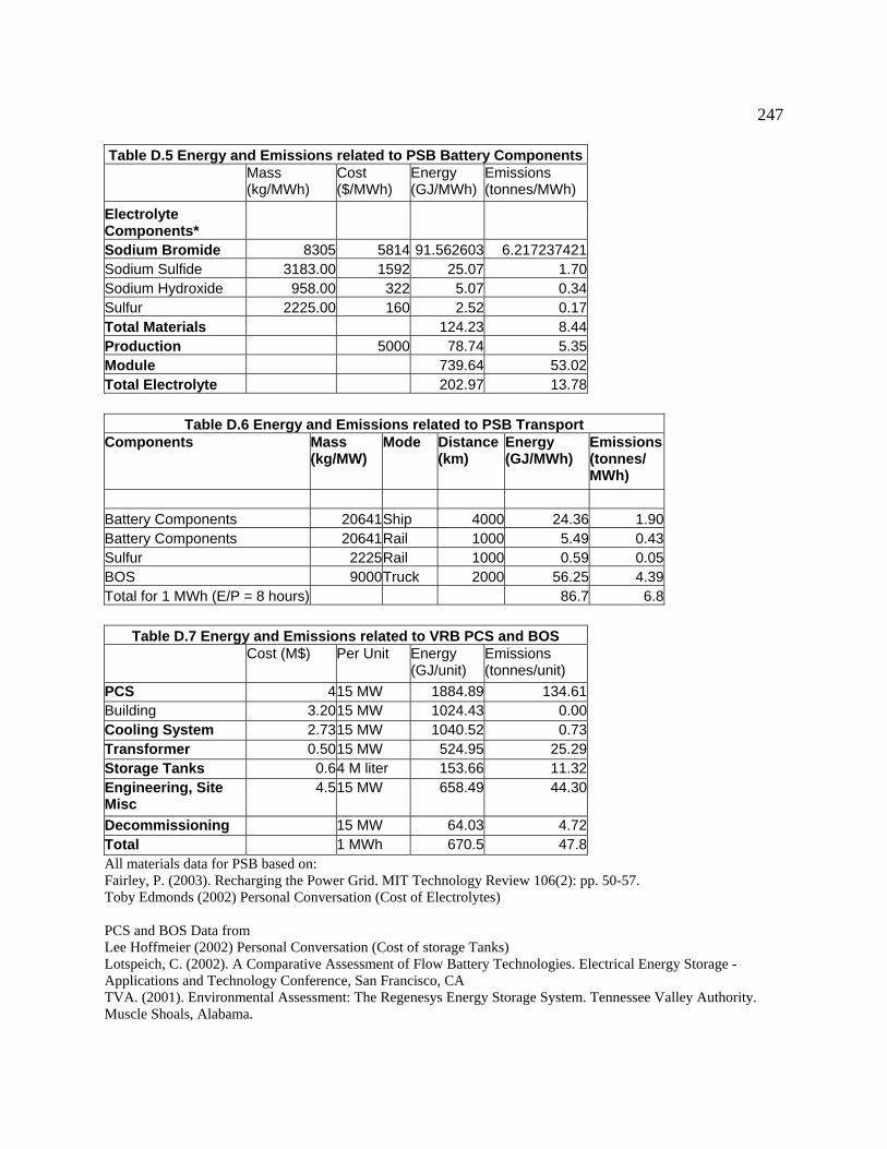
247 Table D.5 Energy and Emissions related to PSB Battery Components

Mass (kg/MWh)

Cost ($/MWh)

Energy (GJ/MWh)


Electrolyte Components* Sodium Bromide 8305 5814 91.562603 6.217237421Sodium Sulfide 3183.00 1592 25.07 1.70Sodium Hydroxide 958.00 322 5.07 0.34Sulfur 2225.00 160 2.52 0.17Total Materials 124.23 8.44Production 5000 78.74 5.35Module 739.64 53.02Total Electrolyte 202.97 13.78

Table D.6 Energy and Emissions related to PSB Transport Components Mass

(kg/MW) Mode Distance



Battery Components 20641Ship 4000 24.36 1.90 Battery Components 20641Rail 1000 5.49 0.43 Sulfur 2225Rail 1000 0.59 0.05 BOS 9000Truck 2000 56.25 4.39 Total for 1 MWh (E/P = 8 hours) 86.7 6.8

Table D.7 Energy and Emissions related to VRB PCS and BOS Cost (M$) Per Unit Energy


PCS 4 15 MW 1884.89 134.61Building 3.20 15 MW 1024.43 0.00Cooling System 2.73 15 MW 1040.52 0.73Transformer 0.50 15 MW 524.95 25.29Storage Tanks 0.6 4 M liter 153.66 11.32Engineering, Site Misc

4.5 15 MW 658.49 44.30

Decommissioning 15 MW 64.03 4.72Total 1 MWh 670.5 47.8All materials data for PSB based on: Fairley, P. (2003). Recharging the Power Grid. MIT Technology Review 106(2): pp. 50-57. Toby Edmonds (2002) Personal Conversation (Cost of Electrolytes) PCS and BOS Data from Lee Hoffmeier (2002) Personal Conversation (Cost of storage Tanks) Lotspeich, C. (2002). A Comparative Assessment of Flow Battery Technologies. Electrical Energy Storage - Applications and Technology Conference, San Francisco, CA TVA. (2001). Environmental Assessment: The Regenesys Energy Storage System. Tennessee Valley Authority. Muscle Shoals, Alabama.

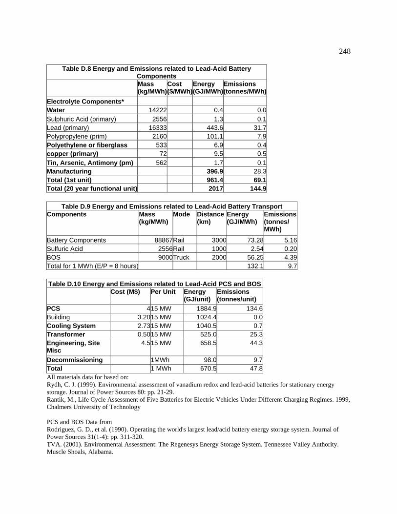
248

Table D.8 Energy and Emissions related to Lead-Acid Battery Components

Mass (kg/MWh)

Cost ($/MWh)

Energy (GJ/MWh)


Electrolyte Components* Water 14222 0.4 0.0Sulphuric Acid (primary) 2556 1.3 0.1Lead (primary) 16333 443.6 31.7Polypropylene (prim) 2160 101.1 7.9Polyethylene or fiberglass 533 6.9 0.4copper (primary) 72 9.5 0.5Tin, Arsenic, Antimony (pm) 562 1.7 0.1Manufacturing 396.9 28.3Total (1st unit) 961.4 69.1Total (20 year functional unit) 2017 144.9

Table D.9 Energy and Emissions related to Lead-Acid Battery Transport Components Mass

(kg/MWh) Mode Distance



Battery Components 88867Rail 3000 73.28 5.16Sulfuric Acid 2556Rail 1000 2.54 0.20BOS 9000Truck 2000 56.25 4.39Total for 1 MWh (E/P = 8 hours) 132.1 9.7 Table D.10 Energy and Emissions related to Lead-Acid PCS and BOS Cost (M$) Per Unit Energy


PCS 4 15 MW 1884.9 134.6Building 3.20 15 MW 1024.4 0.0Cooling System 2.73 15 MW 1040.5 0.7Transformer 0.50 15 MW 525.0 25.3Engineering, Site Misc

4.5 15 MW 658.5 44.3

Decommissioning 1MWh 98.0 9.7Total 1 MWh 670.5 47.8All materials data for based on: Rydh, C. J. (1999). Environmental assessment of vanadium redox and lead-acid batteries for stationary energy storage. Journal of Power Sources 80: pp. 21-29. Rantik, M., Life Cycle Assessment of Five Batteries for Electric Vehicles Under Different Charging Regimes. 1999, Chalmers University of Technology PCS and BOS Data from Rodriguez, G. D., et al. (1990). Operating the world's largest lead/acid battery energy storage system. Journal of Power Sources 31(1-4): pp. 311-320. TVA. (2001). Environmental Assessment: The Regenesys Energy Storage System. Tennessee Valley Authority. Muscle Shoals, Alabama.

249

Appendix E: Calculation of Transmission Line Losses 1: Instantaneous Losses on an AC Line The following example demonstrates estimation of losses that will occur on a proposed transmission line under various operating conditions. Line Details:1

Voltage: 345 kV AC, three-phase Maximum Power Transfer: roughly 1000 MW (typical transfer rates will be lower) Line Length: 370 km Conductor Type: 954 kcmil ACSR “Cardinal”, two conductors/bundle Conductor resistance:2 0.108 ohms/mile at 25C

0.117 ohms/mile at 50C 0.120 ohms/mile at 75C From this information, it is possible to calculate the instantaneous losses. The majority of line losses are due to conductor resistance. Instantaneous power losses in a conductor are given by.

P=I2RT (E.1) where RT is resistance as a function of temperature. Manufacturers data can be used to supply resistance information. Total resistance of a complete line section is calculated by:

/bundleconductors no.

AC) phase-3(for 3 length totallengthohms R total ××= (E.2)

Current in a three-phase power system is calculated from the relationship:

pf3 V

P I××

= (E.3)

where pf is the power factor, assumed to be a constant 0.9 for this estimate. Table E-1 provides instantaneous losses for the line for 3 power transfer cases.

1 Public Service Commission of Wisconsin. Final Environmental Impact Statement Arrowhead – Weston Electric Transmission Line Project – Volume 1 Docket 05-CE-113, October 2000 2 Southwire Corporation. Via http://www.mysouthwire.com/ Accessed July 18, 2003

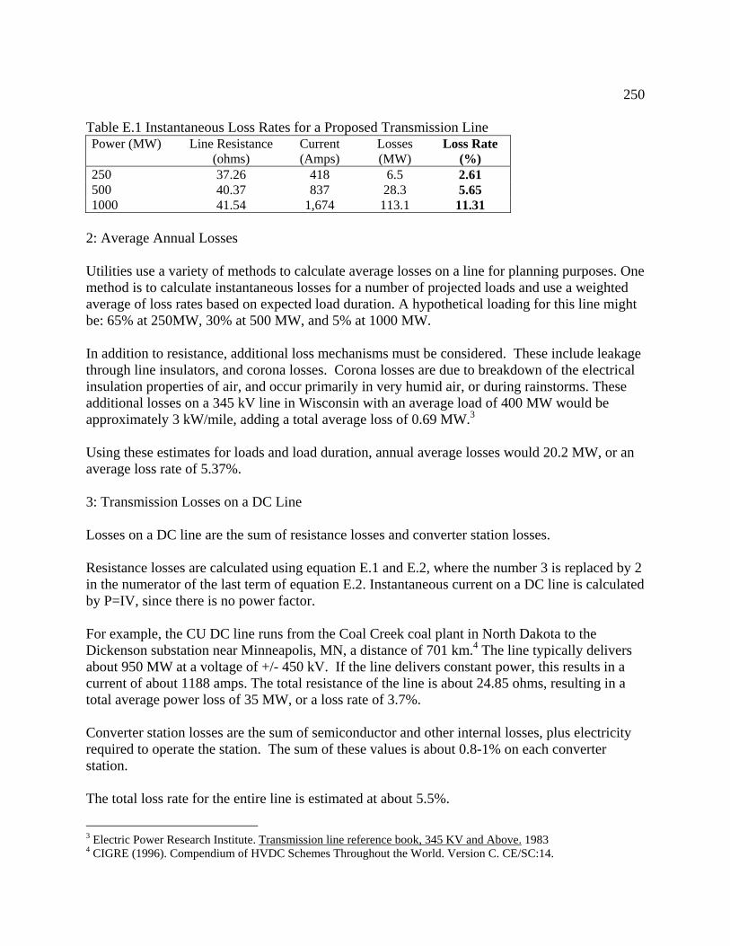
250 Table E.1 Instantaneous Loss Rates for a Proposed Transmission Line Power (MW) Line Resistance

(ohms) Current (Amps)

Losses (MW)

Loss Rate (%)

250 37.26 418 6.5 2.61 500 40.37 837 28.3 5.65 1000 41.54 1,674 113.1 11.31

2: Average Annual Losses Utilities use a variety of methods to calculate average losses on a line for planning purposes. One method is to calculate instantaneous losses for a number of projected loads and use a weighted average of loss rates based on expected load duration. A hypothetical loading for this line might be: 65% at 250MW, 30% at 500 MW, and 5% at 1000 MW. In addition to resistance, additional loss mechanisms must be considered. These include leakage through line insulators, and corona losses. Corona losses are due to breakdown of the electrical insulation properties of air, and occur primarily in very humid air, or during rainstorms. These additional losses on a 345 kV line in Wisconsin with an average load of 400 MW would be approximately 3 kW/mile, adding a total average loss of 0.69 MW.3 Using these estimates for loads and load duration, annual average losses would 20.2 MW, or an average loss rate of 5.37%. 3: Transmission Losses on a DC Line Losses on a DC line are the sum of resistance losses and converter station losses. Resistance losses are calculated using equation E.1 and E.2, where the number 3 is replaced by 2 in the numerator of the last term of equation E.2. Instantaneous current on a DC line is calculated by P=IV, since there is no power factor. For example, the CU DC line runs from the Coal Creek coal plant in North Dakota to the Dickenson substation near Minneapolis, MN, a distance of 701 km.4 The line typically delivers about 950 MW at a voltage of +/- 450 kV. If the line delivers constant power, this results in a current of about 1188 amps. The total resistance of the line is about 24.85 ohms, resulting in a total average power loss of 35 MW, or a loss rate of 3.7%. Converter station losses are the sum of semiconductor and other internal losses, plus electricity required to operate the station. The sum of these values is about 0.8-1% on each converter station. The total loss rate for the entire line is estimated at about 5.5%.

3 Electric Power Research Institute. Transmission line reference book, 345 KV and Above. 1983 4 CIGRE (1996). Compendium of HVDC Schemes Throughout the World. Version C. CE/SC:14.

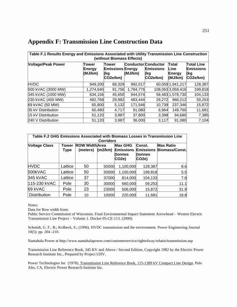
251

Appendix F: Transmission Line Construction Data Table F.1 Results Energy and Emissions Associated with Utility Transmission Line Construction

(without Biomass Effects) Voltage/Peak Power Tower

Energy (MJ/km)

Tower Emissions (kg CO2e/km)

Conductor Energy (MJ/km)

Conductor Emissions (kg CO2e/km)

Total Line Energy (MJ/km)

Total Line Emissions (kg CO2e/km)

HVDC 949,200 68,329 992,017 60,059 1,941,217 128,387500 kVAC (3000 MW) 1,274,640 91,756 1,784,776 108,063 3,059,416 199,818345 kVAC (1000 MW) 634,156 45,650 944,574 58,483 1,578,730 104,133230 kVAC (400 MW) 482,768 29,982 483,444 29,272 966,212 59,25369 kVAC (50 MW) 65,800 5,132 171,546 10,739 237,346 15,87235 kV Distribution 60,480 4,717 91,080 6,964 149,760 11,68115 kV Distribution 51,120 3,987 37,800 3,398 94,680 7,385240 V Distribution 51,120 3,987 36,000 3,117 91,080 7,104

Table F.2 GHG Emissions Associated with Biomass Losses in Transmission Line Corridors

Voltage Class Tower Type

ROW Width(meters)

Area (m2/km)

Max GHG Emissions (tonnes CO2e)

Const. Emissions (tonnes CO2e)

Max Ratio Biomass/Const.

HVDC Lattice 50 50000 1,100,000 128,387 8.6500kVAC Lattice 50 50000 1,100,000 199,818 5.5345 kVAC Lattice 37 37000 814,000 104,133 7.8115-230 kVAC Pole 30 30000 660,000 59,253 11.169 kVAC Pole 23 23000 506,000 15,872 31.9 Distribution Pole 10 10000 220,000 11,681 18.8 Notes: Data for Row width from: Public Service Commission of Wisconsin. Final Environmental Impact Statement Arrowhead – Weston Electric Transmission Line Project – Volume 1. Docket 05-CE-113. (2000). Schmidt, G. F., B.; Kolbeck, S.; (1996). HVDC transmission and the environment. Power Engineering Journal 10(5): pp. 204 -210. Nantahala Power at http://www.nantahalapower.com/customerservice/rightofway/whatis/transmission.asp Transmission Line Reference Book, 345 KV and Above / Second Edition, Copyright 1982 by the Electric Power Research Institute Inc., Prepared by Project UHV. Power Technologies Inc (1978). Transmission Line Reference Book, 115-1389 kV Compact Line Design. Palo Alto, CA, Electric Power Research Institute Inc.

Table F.3 Energy and Emissions Associated with Utility Pole and Tower Construction Voltage Class Type Weight

(kg) Number/kmTower

Energy (MJ/tower)

Tower Emissions (kg CO2e/tower)

Install Cost($)

Install Energy (MJ/tower)

Install Emissions (kg CO2e/tower)

Notes

HVDC Steel Lattice 10500 2.5 361,200 25,946 4,620 18,480 1,386a 500 kv Steel Lattice 14100 2.5 485,040 34,841 6,204 24,816 1,861a 345 kV (single circuit) Steel Lattice 6100 2.875 209,840 15,073 2,684 10,736 805a230 kV Steel Pole 1100 8 58,410 3,603 484 1,936 145a 69 kv Wood Pole 65,800 5,132 b 35 kV Distribution Wood Pole 60,480 4,717 b 15 kV Distribution Wood Pole 51,120 3,987 b Notes: a) Data for Weight, composition and other tower data is Transmission Line Reference Book, 345 KV and Above / Second Edition, Copyright 1982 by the Electric Power Research Institute Inc., Prepared by Project UHV. Install cost based on Ghannoum, E. Y., S.J.; (1989). Optimization of transmission towers and foundations based on their minimum cost. IEEE Transactions on Power Delivery 4(1): pp. 614 -62. b) Data is for 1 km section of wood poles. Data includes entire life-cycle of construction and installation, including 2 poles for wood due to aging Sources: Data is taken from: Kunniger, T. a. K. R. Life Cycle Analysis of Utility Poles, A Swiss Case Study. Proceedings of the 3rd International Wood Preservation Symposium: The Challenge – Safety and Environment (1995). Sedjo, R. Wood materials used as a means to reduce greenhouse gases (GHG): An examination of wooden utility poles.” in Mitigation and Adaptation Strategies for Global Change, Vol. 7, No. 2, 2002, pp191-200, Kluwer Academic Publishers.

Table F.4 Energy and Emissions Associated with Line Conductors

Voltage Peak MVA(approx.)

Conductor Name and number per phase

Size (MCM)

Alum. Weight (kg/km)

Steel Weight (kg/km)

Alum. Energy (MJ/km)

Alum. Emissions (kg CO2e/km)

Steel. Energy (MJ/km)

Steel Emissions (kg CO2e/km)

69 kv 50linnet 336 472 217 49,088 2,885 8,094 694230 kv 400Ortolan 1033 1448 283 150,592 8,852 10,556 906345kv 1000Cardinal use 2/phase 954 1338 490 139,152 8,179 18,277 1,568500 kv 3000bittern use 3/phase 1272 1782 348 185,328 10,893 12,980 1,114HVDC 900kv 1000Lapwing use 2/phase 1590 2229 434 231,816 13,626 16,188 1,389 Notes: Energy and emissions data is for a single conductor! Multiply by number of phases and #of conductors per phase Conductor Data from Walker, M., Ed. (1982). Aluminum Electrical Conductor Handbook, The Aluminum Association. Line Details from Transmission Line Reference Book, 345 KV and Above / Second Edition, Copyright 1982 by the Electric Power Research Institute Inc., Prepared by Project UHV. Power Technologies Inc (1978). Transmission Line Reference Book, 115-1389 kV Compact Line Design. Palo Alto, CA, Electric Power Research Institute Inc.

254

Appendix G: WES Model Flow Diagram

Desired hourly energy

output (ED)

Calculate energy supply deficitESD = EW - ED

ESD = 0

Stock >ABS ESD?

Spare > ESD? Subtract ESD from Stock

Nth hour system output =

Ew + Stock

Calculate spare capacity:Spare =

Capacity - Stock

Add ESD to Stock Stock = Capacity

Nth hour spill =

ESD - Spare

Nth hour system output

= desired output

noyes

noyes

noyes

Stock = 0

Proceed to next hour

Nth hourly wind energy data

(EW)

Stock (energy

currently in storage

Capacity (total energy

storage capacity)

WES Model Flow Diagram. This diagram describes the basic flow of the WES model. In each hour, actual wind output is compared to desired output, and the energy surplus or deficit is met by storage. The amount of energy actually placed into or withdrawn from storage is determined by the storage system energy ratio (ER).

255

Appendix H: Calculation of Life-Cycle Efficiency and GHG Emissions from Wind/PHS and PV/BES Systems

Table H.1 Energy and Emissions Associated with Wind and PHS Subsystems

Const. Energy Input (GJ/MW)

Const. Emissions(tonnes/ MW)

O&M Energy (MJ/MWh)

O&M Emissions (kg CO2e/ MWh)

ER

Wind 8510 769.8 NA NA NA PHS 2984 285.6 25.8 1.8 1.35 Wind Data Includes O&M over lifetime. From White, S. W., and G. L. Kulcinski (2000). Birth to Death Analysis of the Energy Payback Ratio and CO2 Gas Emission Rates from Coal, Fission, Wind, and DT Fusion Electrical Power Plants,. Fusion Engineering and Design 48(248): pp. 473-481.

Table H.2 Life-Cycle Fossil Fuel Efficiency and GHG Emissions Associated with Wind/PHS Systems

Total Annual Energy

Produced (MWh) Fossil Fuel Efficiency

(x100) Life-Cycle GHG Emissions

(kg CO2e/MWh) CF = 0.25 CF = 0.33CF = 0.40CF = 0.25CF = 0.33CF = 0.40CF = 0.25CF = 0.33CF = 0.40Fraction Wind Stored

0 2190 2891 3504 18.5 24.5 29.6 17.6 13.3 11.0

0.10 2133 2816 3413 13.4 17.6 21.4 24.9 18.9 15.6 0.15 2105 2778 3368 13.2 17.4 21.1 25.3 19.3 15.9 0.20 2076 2741 3322 13.0 17.2 20.8 25.8 19.6 16.2 0.25 2048 2703 3277 12.8 16.9 20.5 26.2 20.0 16.6 0.30 2020 2666 3231 12.7 16.7 20.2 26.7 20.3 16.9 0.35 1991 2628 3186 12.5 16.5 20.0 27.1 20.7 17.2 0.40 1963 2591 3141 12.3 16.2 19.7 27.6 21.1 17.5 0.45 1935 2554 3095 12.1 16.0 19.4 28.1 21.5 17.9 0.50 1906 2516 3050 11.9 15.8 19.1 28.6 21.9 18.2

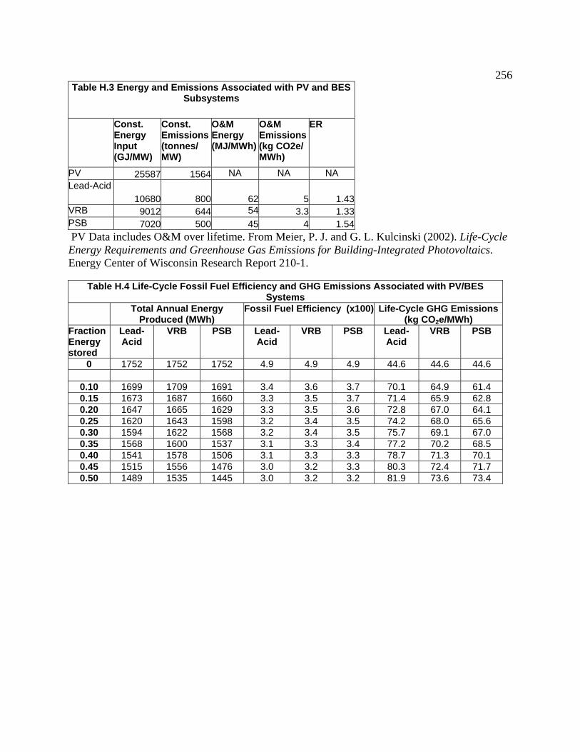
256Table H.3 Energy and Emissions Associated with PV and BES

Subsystems

Const. Energy Input (GJ/MW)

Const. Emissions (tonnes/ MW)

O&M Energy (MJ/MWh)

O&M Emissions (kg CO2e/ MWh)

ER

PV 25587 1564 NA NA NA Lead-Acid

10680 800 62 5 1.43VRB 9012 644 54 3.3 1.33PSB 7020 500 45 4 1.54 PV Data includes O&M over lifetime. From Meier, P. J. and G. L. Kulcinski (2002). Life-Cycle Energy Requirements and Greenhouse Gas Emissions for Building-Integrated Photovoltaics. Energy Center of Wisconsin Research Report 210-1.

Table H.4 Life-Cycle Fossil Fuel Efficiency and GHG Emissions Associated with PV/BES Systems

Total Annual Energy

Produced (MWh) Fossil Fuel Efficiency (x100) Life-Cycle GHG Emissions

(kg CO2e/MWh) Fraction Energy stored

Lead-Acid

VRB PSB Lead- Acid

VRB PSB Lead-Acid

VRB PSB

0 1752 1752 1752 4.9 4.9 4.9 44.6 44.6 44.6

0.10 1699 1709 1691 3.4 3.6 3.7 70.1 64.9 61.4 0.15 1673 1687 1660 3.3 3.5 3.7 71.4 65.9 62.8 0.20 1647 1665 1629 3.3 3.5 3.6 72.8 67.0 64.1 0.25 1620 1643 1598 3.2 3.4 3.5 74.2 68.0 65.6 0.30 1594 1622 1568 3.2 3.4 3.5 75.7 69.1 67.0 0.35 1568 1600 1537 3.1 3.3 3.4 77.2 70.2 68.5 0.40 1541 1578 1506 3.1 3.3 3.3 78.7 71.3 70.1 0.45 1515 1556 1476 3.0 3.2 3.3 80.3 72.4 71.7 0.50 1489 1535 1445 3.0 3.2 3.2 81.9 73.6 73.4

257

Appendix I: Performance of Existing Coal Plants in the Midwestern U.S. Used in this Study EPA eGRID2002 Version 2.01 Plant File (Year 2000 Data) State Plant name Plant

capacity factor

Plant generator capacity (MW)

Plant 2000 annual NOx input emission rate (lbs/MMBtu)

Plant 2000 annual SO2 input emission rate (lbs/MMBtu)

Plant 2000 nominal heat rate (Btu/kWh)

OH O H HUTCHINGS 0.2260 447 0.588 1.258 11,967 PA CROMBY 0.2422 420 0.343 0.800 13,819 PA EDDYSTONE 0.2469 1569 0.264 0.404 13,181 KY TYRONE 0.2477 138 0.654 1.250 13,981 MI HARBOR BEACH 0.2601 125 0.921 1.344 11,740 MI DAN E KARN 0.2930 1761 0.326 0.896 11,690 IN LOGANSPORT 0.2990 61 0.871 2.380 14,543 KY E W BROWN 0.3212 1606 0.389 1.991 11,205 WV NORTH BRANCH 0.3212 80 0.356 0.311 14,676 OH PAINESVILLE 0.3351 54 0.866 3.006 15,205 PA PORTLAND 0.3410 620 0.271 2.173 10,080 PA SEWARD 0.3850 218 0.440 2.551 11,605 IN DEAN H MITCHELL 0.3917 547 0.272 0.551 12,317 IN NOBLESVILLE 0.4009 100 0.972 3.116 12,563 IN ELMER W STOUT 0.4039 1000 0.333 2.085 10,928 OH R E BURGER 0.4128 538 0.679 4.605 10,560 OH ORRVILLE 0.4155 85 0.956 6.642 15,462 IN EDWARDSPORT 0.4176 144 0.696 2.630 15,552 IN H T PRITCHARD 0.4242 396 0.515 2.045 11,727

PA MITCHELL POWER STATION 0.4337 449 0.370 0.141 11,085

PA NEW CASTLE PLANT 0.4343 431 0.378 2.547 11,819 MI ST CLAIR 0.4354 1929 0.478 1.256 10,896

PA SUNBURY GENERATION LLC 0.4443 498 0.565 2.439 11,875

OH PICWAY 0.4504 106 0.483 4.484 11,238 KY GREEN RIVER 0.4518 264 0.578 3.380 13,246 MI ECKERT STATION 0.4557 375 0.381 0.646 13,805 IN MICHIGAN CITY 0.4610 680 0.512 0.739 11,139 OH NILES 0.4647 293 0.929 2.991 11,136 OH EASTLAKE 0.4657 1289 0.562 2.252 10,571 KY HMP&L STATION TWO 0.4682 405 0.472 0.460 15,442 IN BAILLY 0.4933 653 1.308 0.323 11,282 IN WABASH RIVER 0.4942 1173 0.439 2.115 10,906 MI J B SIMS 0.4975 85 0.388 0.324 10,438

258State Plant name Plant

capacity factor





PA ELRAMA POWER PLANT 0.4997 510 0.482 0.308 13,470

MI B C COBB 0.4999 511 0.348 1.275 11,286 IN R M SCHAHFER 0.5063 2201 0.384 0.635 11,275 OH BAY SHORE 0.5159 655 0.734 0.580 10,552 WV RIVESVILLE 0.5389 110 0.783 1.711 13,249 KY SHAWNEE 0.5506 1750 0.380 0.658 12,280 IN A B BROWN 0.5516 619 0.435 0.435 10,547 KY CANE RUN 0.5552 661 0.411 0.929 11,676 PA TITUS 0.5616 261 0.315 2.246 10,624

MI ENDICOTT GENERATING 0.5622 55 0.399 0.376 14,831

OH CONESVILLE 0.5685 2175 0.529 2.525 10,088 OH W H SAMMIS 0.5855 2468 0.503 1.847 10,320 KY PARADISE 0.5870 2558 0.867 2.039 10,815 PA SHAWVILLE 0.5951 631 0.425 2.863 10,246 WV JOHN E AMOS 0.5990 2933 0.590 1.223 9,683 KY MILL CREEK 0.6005 1717 0.379 0.640 11,942 PA HOMER CITY STATION 0.6043 2194 0.442 2.188 10,333 IN TANNERS CREEK 0.6054 1100 1.121 2.315 9,989

PA G F WEATON POWER STATION 0.6065 120 0.561 0.390 11,626

OH WALTER C BECKJORD 0.6100 1376 0.547 1.798 10,825 MI J H CAMPBELL 0.6151 1542 0.499 0.956 10,262 KY GREEN STATION 0.6158 586 0.424 0.196 10,935 OH W H ZIMMER 0.6173 1426 0.472 0.491 10,266 WV MITCHELL 0.6175 1633 0.581 1.268 9,641 KY COOPER 0.6182 321 0.427 1.976 10,546 MI JAMES DE YOUNG 0.6187 63 0.648 1.270 14,001 WV ALBRIGHT 0.6221 278 0.507 2.475 12,139 MI BELLE RIVER 0.6231 1709 0.268 0.554 11,371 WV PLEASANTS 0.6240 1368 0.358 1.110 9,891 OH MUSKINGUM RIVER 0.6274 1530 0.706 3.876 9,578 MI MONROE 0.6362 3293 0.534 1.220 9,606 IN R GALLAGHER 0.6365 600 0.432 3.393 10,397 WV KANAWHA RIVER 0.6369 439 0.615 1.210 9,967 KY GHENT 0.6378 2226 0.356 0.882 10,791 WV MOUNTAINEER (1301) 0.6449 1300 0.505 1.087 9,604

PA CHESWICK POWER PLANT 0.6454 565 0.366 2.575 10,919

PA HATFIELD'S FERRY POWER STATION 0.6474 1728 0.473 3.375 10,019

259State Plant name Plant

capacity factor





IN WHITEWATER VALLEY 0.6495 94 0.434 3.611 12,514

PA

ST NICHOLAS COGENERATION PROJECT 0.6514 117 2.069 0.718 12,421

MI ERICKSON 0.6534 155 0.419 1.379 10,650 MI J R WHITING 0.6622 346 0.309 0.887 11,668 OH CARDINAL 0.6632 1880 0.564 2.346 9,316 KY ELMER SMITH 0.6772 445 0.759 0.410 12,646 PA BRUCE MANSFIELD 0.6831 2741 0.370 0.372 9,535 OH J M STUART 0.6845 2452 0.591 1.443 9,963 WV KAMMER 0.6891 713 0.769 2.149 9,283 IN STATE LINE ENERGY 0.6899 532 0.595 0.559 10,014 OH MIAMI FORT 0.7021 1358 0.563 1.795 10,874 KY TRIMBLE COUNTY 0.7031 566 0.393 0.415 10,494 WV PHIL SPORN 0.7039 1106 0.622 1.696 9,367 IN MEROM 0.7244 1080 0.386 0.401 12,252 OH GEN J M GAVIN 0.7268 2600 0.483 0.281 10,625 IN PETERSBURG 0.7271 1881 0.335 0.626 11,214

KY KENNETH C COLEMAN STATION 0.7273 521 0.431 2.516 10,816

WV ALLOY STEAM STATION 0.7285 40 0.906 0.438 12,597

IN GIBSON 0.7297 3340 0.446 1.599 10,045 PA KEYSTONE 0.7309 1883 0.327 2.755 9,242 PA CONEMAUGH 0.7324 1883 0.342 0.118 9,954 IN CLIFTY CREEK 0.7328 1304 0.753 1.008 10,117 KY BIG SANDY 0.7410 1097 0.540 1.550 9,388 IN F B CULLEY 0.7506 411 0.461 0.733 11,860 KY DALE 0.7528 176 0.491 1.249 11,399 WV HARRISON 0.7534 2052 0.469 0.088 10,585 MI J C WEADOCK 0.7534 333 0.306 0.814 10,744 OH KILLEN STATION 0.7636 687 0.454 1.059 10,126 KY EAST BEND 0.7670 648 0.381 0.653 10,446 WV FORT MARTIN 0.7767 1152 0.715 2.445 9,400 IN ROCKPORT 0.7874 2600 0.406 0.696 10,154 WV MT STORM 0.7900 1681 0.624 1.825 10,652 WV WILLOW ISLAND 0.7956 213 1.076 2.097 11,774

WV GRANT TOWN POWER PLANT 0.8107 96 1.004 0.348 12,465

IN FRANK E RATTS 0.8169 233 0.491 2.505 11,028 KY D B WILSON STATION 0.8270 440 0.435 0.504 12,580 OH KYGER CREEK 0.8413 1086 0.781 3.303 9,546

UWFDM-1410 Environmental and Policy Analysis of Renewable

Documents

Transcript of UWFDM-1410 Environmental and Policy Analysis of Renewable