•

W I S C O N SI N

•

FU

SIO

N•

TECHNOLOGY• INS

TIT

UT

E

FUSION TECHNOLOGY INSTITUTE

UNIVERSITY OF WISCONSIN

MADISON WISCONSIN

Monte Carlo Isotopic Inventory Analysis forComplex Nuclear Systems

Phiphat Phruksarojanakun

January 2007

UWFDM-1323

Ph.D. thesis.

Monte Carlo Isotopic Inventory Analysis for

Complex Nuclear Systems

Phiphat Phruksarojanakun

Fusion Technology InstituteUniversity of Wisconsin1500 Engineering Drive

Madison, WI 53706

http://fti.neep.wisc.edu

January 2007

UWFDM-1323

Ph.D. thesis.

MONTE CARLO ISOTOPIC INVENTORY ANALYSIS FOR

COMPLEX NUCLEAR SYSTEMS

by

Phiphat Phruksarojanakun

A dissertation submitted in partial fulfillment of

the requirements for the degree of

Doctor of Philosophy

(Nuclear Engineering and Engineering Physics )

at the

UNIVERSITY OF WISCONSIN – MADISON

2007

i

ABSTRACT

Monte Carlo Inventory Simulation Engine or MCise is a newly developed method for

calculating isotopic inventory of materials. The method offers the promise of modeling

materials with complex processes and irradiation histories, which pose challenges for current

deterministic tools. Monte Carlo techniques based on following the history of individual

atoms allows those atoms to follow randomly determined flow paths, enter or leave the system

at arbitrary locations, and be subjected to radiation or chemical processes at different points

in the flow path.

The method has strong analogies to Monte Carlo neutral particle transport. The funda-

mental of analog method is fully developed, including considerations for simple, complex and

loop flows. The validity of the analog method is demonstrated with test problems under var-

ious flow conditions. The method reproduces the results of a deterministic inventory code for

comparable problems. While a successful and efficient parallel implementation has permit-

ted an inexpensive way to improve statistical precision by increasing the number of sampled

atoms, this approach does not always provide the most efficient avenue for improvement.

Therefore, six variance reduction tools are implemented as alternatives to improve precision

of Monte Carlo simulations. Forced Reaction is designed to force an atom to undergo a pre-

defined number of reactions in a given irradiation environment. Biased Reaction Branching

is primarily focused on improving statistical results of the isotopes that are produced from

rare reaction pathways. Biased Source Sampling is aimed at increasing frequencies of sam-

pling rare initial isotopes as the starting particles. Reaction Path Splitting increases the

population by splitting the atom at each reaction point, creating one new atom for each de-

cay or transmutation product. Delta Tracking is recommended for a high-frequency pulsing

ii

to greatly reduce the computing time. Lastly, Weight Window is introduced as a strategy

to decrease large deviations of weight due to the uses of variance reduction techniques.

A figure of merit is necessary to evaluate the efficiency of a variance reduction technique.

A number of possibilities for the figure of merit are explored, two of which offer robust figures

of merit. One figure of merit is based on the relative error of a known target isotope (1/R2T )

and another on the overall detection limit corrected by the relative error (1/DkR2T ). An

automated Adaptive Variance-reduction Adjustment (AVA) tool is developed to iteratively

define necessary parameters for some variance reduction techniques in a problem with a

target isotope. Initial sample problems demonstrate that AVA improves both precision and

accuracy of a target result in an efficient manner.

Potential applications of MCise include molten salt fueled reactors and liquid breeders in

fusion blankets. As an example, the inventory analysis of an actinide fluoride eutectic liquid

fuel in the In-Zinerator, a sub-critical power reactor driven by a fusion source, is examined

using MCise. The result reassures MCise as a reliable tool for inventory analysis of complex

nuclear systems.

iii

Dedicated to my late grandfather,

Silapachai Phruksarojanakun.

1920–2006

iv

ACKNOWLEDGEMENTS

I would like to extend my greatest gratitude and regard to my advisor, Professor Paul

Wilson, for years of invaluable advice and guidance on this work. I have learned a great

deal from his methodical analysis and engineering judgment which I can never learn in the

classroom.

Sincere thanks are given to individuals in the Department of Engineering Physics, espe-

cially those in Fusion Technology Institute (FTI), who have helped me during the course of

my study. Tony Hammond has done a good job keeping a cluster active. Milad Fatenejad

has been a reliable person to talk to when I struggle with a programming problem. I would

also like to thank Professor Douglass Henderson, Dr. Timothy Tautges, Research Professor

Laila El-Guebaly and Research Professor Mohamed Sawan for all their help.

I would like to thank my friends who have made my stay in Madison a memorable

experience. Thanks to the wonderful people from the Badminton Club, I am fortunate

enough to know and hang out with them. I feel privileged to be a part of this university

from which I have learned so much. Though the Badgers sports let me down at times, they

are always fun to watch. I will forever be a Badgers fan. On Wisconsin!

Finally, I would like to express my deepest thank to the Suns family, my grandmother,

mother, father, brothers Phichat and Phinat and a very special person, Tulaya Limpiti, for

the endless love and support they have given me. Without their encouragement, I would not

have reached my goal. I am deeply grateful to have the family that I have.

v

TABLE OF CONTENTS

Page

ABSTRACT . . . . . . . . . . . . . . . . . . . . . . . . . . . . . . . . . . . . . . . i

ACKNOWLEDGEMENTS . . . . . . . . . . . . . . . . . . . . . . . . . . . . . . iv

LIST OF TABLES . . . . . . . . . . . . . . . . . . . . . . . . . . . . . . . . . . . . ix

LIST OF FIGURES . . . . . . . . . . . . . . . . . . . . . . . . . . . . . . . . . . . xi

1 Introduction . . . . . . . . . . . . . . . . . . . . . . . . . . . . . . . . . . . . . 1

1.1 Overview on Traditional Methods . . . . . . . . . . . . . . . . . . . . . . . . 21.2 Overview of a Monte Carlo Method . . . . . . . . . . . . . . . . . . . . . . . 51.3 Advantages of a Monte Carlo Method in Isotopic Inventory . . . . . . . . . . 71.4 Goals . . . . . . . . . . . . . . . . . . . . . . . . . . . . . . . . . . . . . . . . 7

2 Analog Monte Carlo Isotopic Inventory . . . . . . . . . . . . . . . . . . . . 10

2.1 Introduction . . . . . . . . . . . . . . . . . . . . . . . . . . . . . . . . . . . . 102.2 Methodology . . . . . . . . . . . . . . . . . . . . . . . . . . . . . . . . . . . 10

2.2.1 Problem Formulation . . . . . . . . . . . . . . . . . . . . . . . . . . . 112.2.2 Basic Elements . . . . . . . . . . . . . . . . . . . . . . . . . . . . . . 122.2.3 Enabling Concepts . . . . . . . . . . . . . . . . . . . . . . . . . . . . 142.2.4 Compound Capabilities . . . . . . . . . . . . . . . . . . . . . . . . . . 162.2.5 Relationship to Monte Carlo neutral particle transport . . . . . . . . 19

2.3 Testing . . . . . . . . . . . . . . . . . . . . . . . . . . . . . . . . . . . . . . . 202.3.1 Single Control Volume: 0-D Analytic and Numerical . . . . . . . . . 202.3.2 Simple, Complex and Loop Flow . . . . . . . . . . . . . . . . . . . . 252.3.3 Sources, Tallies, Decay and Sinks . . . . . . . . . . . . . . . . . . . . 272.3.4 Parallel Performance . . . . . . . . . . . . . . . . . . . . . . . . . . . 33

2.4 Summary . . . . . . . . . . . . . . . . . . . . . . . . . . . . . . . . . . . . . 35

vi

Page

3 Variance Reduction Techniques . . . . . . . . . . . . . . . . . . . . . . . . . 36

3.1 Introduction . . . . . . . . . . . . . . . . . . . . . . . . . . . . . . . . . . . . 363.2 Forced Reaction . . . . . . . . . . . . . . . . . . . . . . . . . . . . . . . . . . 37

3.2.1 Methodology . . . . . . . . . . . . . . . . . . . . . . . . . . . . . . . 373.2.2 Test Problems . . . . . . . . . . . . . . . . . . . . . . . . . . . . . . . 393.2.3 Simulation Results . . . . . . . . . . . . . . . . . . . . . . . . . . . . 40

3.3 Biased Reaction Branching . . . . . . . . . . . . . . . . . . . . . . . . . . . . 423.3.1 Methodology . . . . . . . . . . . . . . . . . . . . . . . . . . . . . . . 433.3.2 Test Problems . . . . . . . . . . . . . . . . . . . . . . . . . . . . . . . 443.3.3 Simulation Results . . . . . . . . . . . . . . . . . . . . . . . . . . . . 45

3.4 Biased Source Sampling . . . . . . . . . . . . . . . . . . . . . . . . . . . . . 483.4.1 Methodology . . . . . . . . . . . . . . . . . . . . . . . . . . . . . . . 483.4.2 Test Problems . . . . . . . . . . . . . . . . . . . . . . . . . . . . . . . 493.4.3 Simulation Results . . . . . . . . . . . . . . . . . . . . . . . . . . . . 49

3.5 Reaction Path Splitting . . . . . . . . . . . . . . . . . . . . . . . . . . . . . . 513.5.1 Methodology . . . . . . . . . . . . . . . . . . . . . . . . . . . . . . . 513.5.2 Test Problem . . . . . . . . . . . . . . . . . . . . . . . . . . . . . . . 523.5.3 Simulation Results . . . . . . . . . . . . . . . . . . . . . . . . . . . . 52

3.6 Weight Window . . . . . . . . . . . . . . . . . . . . . . . . . . . . . . . . . . 553.6.1 Development Scope . . . . . . . . . . . . . . . . . . . . . . . . . . . . 553.6.2 Methodology . . . . . . . . . . . . . . . . . . . . . . . . . . . . . . . 563.6.3 Testing . . . . . . . . . . . . . . . . . . . . . . . . . . . . . . . . . . . 57

3.7 Delta Tracking . . . . . . . . . . . . . . . . . . . . . . . . . . . . . . . . . . 603.7.1 Methodology . . . . . . . . . . . . . . . . . . . . . . . . . . . . . . . 613.7.2 Test Problems . . . . . . . . . . . . . . . . . . . . . . . . . . . . . . . 633.7.3 Simulation Results . . . . . . . . . . . . . . . . . . . . . . . . . . . . 64

3.8 Summary . . . . . . . . . . . . . . . . . . . . . . . . . . . . . . . . . . . . . 66

4 Figures of Merit . . . . . . . . . . . . . . . . . . . . . . . . . . . . . . . . . . . 68

4.1 Introduction and Importance of Figure of Merit . . . . . . . . . . . . . . . . 684.2 Principles and Constraints of Figure of Merit . . . . . . . . . . . . . . . . . . 694.3 Development of Figures of Merit . . . . . . . . . . . . . . . . . . . . . . . . . 70

4.3.1 Statistical Error of Single Result (1 / R2T) . . . . . . . . . . . . . . . 714.3.2 Number of Qualified Isotopes (Nk) . . . . . . . . . . . . . . . . . . . 744.3.3 Detection Limit (1 /DkT ) . . . . . . . . . . . . . . . . . . . . . . . . 754.3.4 Error Corrected Detection Limit (1/DkR

2T ) . . . . . . . . . . . . . . 784.4 Summary . . . . . . . . . . . . . . . . . . . . . . . . . . . . . . . . . . . . . 80

vii

Page

5 Efficiency Assessment . . . . . . . . . . . . . . . . . . . . . . . . . . . . . . . 81

5.1 Problem Definitions . . . . . . . . . . . . . . . . . . . . . . . . . . . . . . . . 815.1.1 Standard test problem . . . . . . . . . . . . . . . . . . . . . . . . . . 815.1.2 Study problem 1 . . . . . . . . . . . . . . . . . . . . . . . . . . . . . 815.1.3 Study problem 2 . . . . . . . . . . . . . . . . . . . . . . . . . . . . . 82

5.2 Simulation Results . . . . . . . . . . . . . . . . . . . . . . . . . . . . . . . . 825.2.1 Study problem 1 . . . . . . . . . . . . . . . . . . . . . . . . . . . . . 825.2.2 Study Problem 2 . . . . . . . . . . . . . . . . . . . . . . . . . . . . . 87

5.3 Summary . . . . . . . . . . . . . . . . . . . . . . . . . . . . . . . . . . . . . 90

6 AVA: Adaptive Variance-reduction Adjustment . . . . . . . . . . . . . . . 91

6.1 Algorithm . . . . . . . . . . . . . . . . . . . . . . . . . . . . . . . . . . . . . 936.1.1 Forced Reaction . . . . . . . . . . . . . . . . . . . . . . . . . . . . . . 956.1.2 Biased Reaction Branching . . . . . . . . . . . . . . . . . . . . . . . . 956.1.3 Biased Source Sampling . . . . . . . . . . . . . . . . . . . . . . . . . 97

6.2 Sample Problems . . . . . . . . . . . . . . . . . . . . . . . . . . . . . . . . . 986.3 Results and Discussions . . . . . . . . . . . . . . . . . . . . . . . . . . . . . 986.4 Summary . . . . . . . . . . . . . . . . . . . . . . . . . . . . . . . . . . . . . 104

7 Applications . . . . . . . . . . . . . . . . . . . . . . . . . . . . . . . . . . . . . 105

7.1 Coolant Activation . . . . . . . . . . . . . . . . . . . . . . . . . . . . . . . . 1057.1.1 Problem Modifications . . . . . . . . . . . . . . . . . . . . . . . . . . 1067.1.2 MCise Simulation . . . . . . . . . . . . . . . . . . . . . . . . . . . . . 1077.1.3 Numerical Result . . . . . . . . . . . . . . . . . . . . . . . . . . . . . 109

7.2 In-Zinerator . . . . . . . . . . . . . . . . . . . . . . . . . . . . . . . . . . . . 1127.2.1 MCise Simulation . . . . . . . . . . . . . . . . . . . . . . . . . . . . . 1137.2.2 Analysis Methodology . . . . . . . . . . . . . . . . . . . . . . . . . . 1177.2.3 Results and Discussion . . . . . . . . . . . . . . . . . . . . . . . . . . 119

7.3 ARIES-CS . . . . . . . . . . . . . . . . . . . . . . . . . . . . . . . . . . . . . 1237.3.1 MCise Simulation . . . . . . . . . . . . . . . . . . . . . . . . . . . . . 1237.3.2 Numerical Results . . . . . . . . . . . . . . . . . . . . . . . . . . . . 1257.3.3 Statistical Improvement Using ALARA-based AVA . . . . . . . . . . 127

8 Future Research and Summary . . . . . . . . . . . . . . . . . . . . . . . . . 131

8.1 Weight Window Development . . . . . . . . . . . . . . . . . . . . . . . . . . 1318.2 Analog Delta Tracking . . . . . . . . . . . . . . . . . . . . . . . . . . . . . . 132

viii

Page

8.3 Automated ALARA-based AVA . . . . . . . . . . . . . . . . . . . . . . . . . 1338.4 Research Summary . . . . . . . . . . . . . . . . . . . . . . . . . . . . . . . . 134

BIBLIOGRAPHY . . . . . . . . . . . . . . . . . . . . . . . . . . . . . . . . . . . . 136

ix

LIST OF TABLES

Table Page

2.1 Contributions to different tally types from sample reaction sequence shown inFigure 2.2. . . . . . . . . . . . . . . . . . . . . . . . . . . . . . . . . . . . . . . 17

2.2 Analogies between elements of Monte Carlo neutral particle transport and MonteCarlo inventory analysis. . . . . . . . . . . . . . . . . . . . . . . . . . . . . . . . 19

2.3 Comparing improvements in results (relative to deterministic calculation) andstatistical error with increasing number of initial atoms. . . . . . . . . . . . . . 23

2.4 Summary of computing efficiency as different numbers of processors were used onthe same problem. Nearly 100% parallel efficiency can be achieved for problemsof fixed total work. . . . . . . . . . . . . . . . . . . . . . . . . . . . . . . . . . . 34

2.5 Constant run-time can be achieved for problems with fixed work per processor. 34

3.1 Comparisons of different characteristic numbers of products between the analyt-ical result and Monte Carlo results governed by six forced reaction parameters.The mean reative differences and mean statistical errors are derived from twenty-six isotopes common in all cases. . . . . . . . . . . . . . . . . . . . . . . . . . . 41

3.2 Comparisons of different characteristic numbers of products between the analogresult and the results from a uniform reaction branching. The mean relativedifferences and mean statistical errors are derived from those with statisticalerror less than 5% in each case. . . . . . . . . . . . . . . . . . . . . . . . . . . . 45

3.3 Quantitative comparisons of different characteristic numbers of products betweenthe analog result and the results from a reaction path splitting. The mean relativedifferences and mean statistical errors are derived from those with statistical errorless than 10% in each case. . . . . . . . . . . . . . . . . . . . . . . . . . . . . . 54

3.4 Summary of characteristics of the results from the simulations with differentdefinitions of weight window. . . . . . . . . . . . . . . . . . . . . . . . . . . . . 59

x

Table Page

5.1 The values of figure of merit (1/R2T ) were calculated from nine test runs and theanalog problem (1010 particles for case 0) when 51Cr was a target isotope. Thevalues of one-percent error corrected detection limit (1/D1R

2T ) were included tocompare the general efficiencies of all test cases. One million simulated particleswere used for each test problem. . . . . . . . . . . . . . . . . . . . . . . . . . . 83

5.2 Reaction channels leading to the most productions of 49Ti, 53Mn and 60Ni weredescribed and used for estimating the optimal values of variance reduction pa-rameters. . . . . . . . . . . . . . . . . . . . . . . . . . . . . . . . . . . . . . . . 84

5.3 The most efficient configurations of variance reduction parameters for detectingthree isotopes in the study cases are shown. . . . . . . . . . . . . . . . . . . . . 87

5.4 Comparisons of relative error, computing time and FOM between an analogproblem and study cases with optimal sets of variance reduction parameters areshown. Improvements in all areas from the analog problem are observed in allcases. . . . . . . . . . . . . . . . . . . . . . . . . . . . . . . . . . . . . . . . . . 88

5.5 Comparison of some characteristics of the results from the six study cases withdifferent force parameter. . . . . . . . . . . . . . . . . . . . . . . . . . . . . . . 88

7.1 Residence times in the core, reactor and outer circuit, and relative volumetricflow rates in the core and reactor are assumed. . . . . . . . . . . . . . . . . . . 108

7.2 Isotopic compositions of sources used in the MCise simulation are shown. . . . . 115

7.3 Values for six parameters necessary for the MCise simulation are assumed andshown. . . . . . . . . . . . . . . . . . . . . . . . . . . . . . . . . . . . . . . . . . 117

7.4 Isotopic compositions of the LiPb liquid breeder. Li is 90-percent enrichmentwith 6Li. The theoretical density is 8.80 g/cm3. . . . . . . . . . . . . . . . . . . 124

xi

LIST OF FIGURES

Figure Page

1.1 A simple example of mixing flow paths. Two flows of coolant coming from a hardand soft spectrum region mix in the heat exchanger and re-enter the reactor. . . 4

2.1 Four different flow and complexity regimes: a) 0-D b) simple flow c) complexflow, d) loop flow. . . . . . . . . . . . . . . . . . . . . . . . . . . . . . . . . . . 13

2.2 Representative reaction sequence between points of time to illustrate differencebetween current and population tallies. . . . . . . . . . . . . . . . . . . . . . . . 17

2.3 An arbitrary flow system (with complex and loop flows) representing a simplifiedtwo region coolant (A1 and A2) with chemical cleaning step (C) following theheat exchanger (B). In addition to the 40/60 flow split between regions A1 andA2, 5% of the flow leaving the heat exchanger is diverted to the cleanup system. 18

2.4 Comparison of Monte Carlo results to analytic benchmark results showing goodagreement. Since the half life of 14O was 70.60 seconds long, an initial unitamount of 14O was reduced to a half and a quarter after 70.60 seconds and141.20 seconds, respectively. . . . . . . . . . . . . . . . . . . . . . . . . . . . . . 21

2.5 Variation of relative difference between Monte Carlo (MC) and deterministicresults as a function of the deterministic result. The expected statistical error(2σ) as a function of the result is also shown for a MC problem with 1010 initialatoms. Results with a 1σ statistical error greater than 5% are shown with opensymbols (¦). . . . . . . . . . . . . . . . . . . . . . . . . . . . . . . . . . . . . . . 21

2.6 The average ratio (averaged over all isotopes) improves with more atom histo-ries. The statistical error of the average is the root-mean-squared average of theindividual statistical errors and is shown here as a 1σ statistical error. . . . . . 23

2.7 Physically equivalent/comparable test cases for testing flow capabilities. . . . . 26

xii

Figure Page

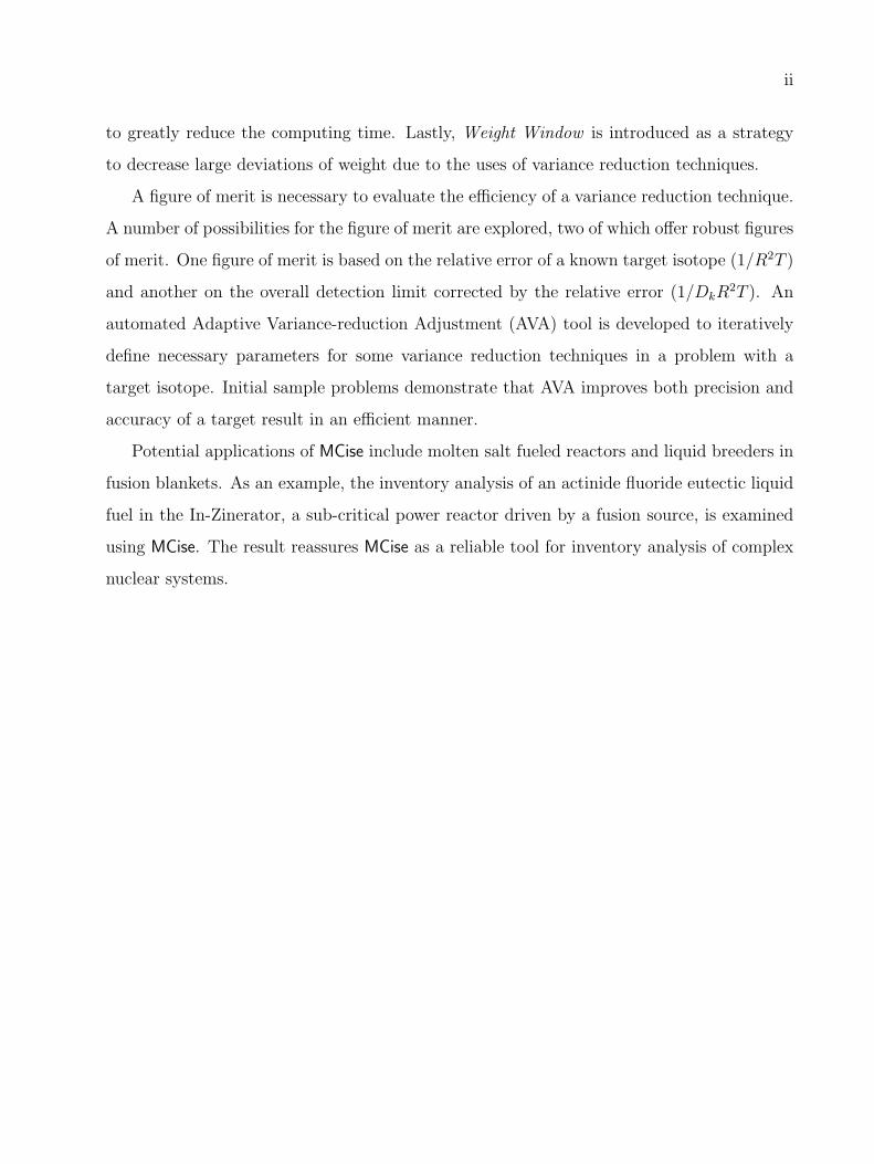
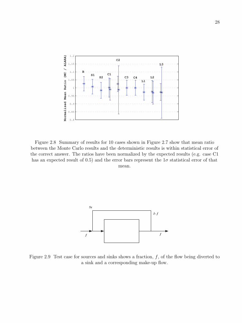
2.8 Summary of results for 10 cases shown in Figure 2.7 show that mean ratio betweenthe Monte Carlo results and the deterministic results is within statistical errorof the correct answer. The ratios have been normalized by the expected results(e.g. case C1 has an expected result of 0.5) and the error bars represent the 1σstatistical error of that mean. . . . . . . . . . . . . . . . . . . . . . . . . . . . . 28

2.9 Test case for sources and sinks shows a fraction, f , of the flow being diverted toa sink and a corresponding make-up flow. . . . . . . . . . . . . . . . . . . . . . 28

2.10 Relative isotopic inventories for a select sample of isotopes. Declining transmu-tation rates accompany a higher loss rate in source/sink problems because theaverage atom spends less time in the neutron flux. . . . . . . . . . . . . . . . . 29

2.11 A comparison of relative difference as a function of the benchmark result com-pared to the statistical error shows agreement for values of f=0, 0.5, and 1. . . 32

2.12 Relative difference as a function of deterministic result for shutdown and twodifference cooling times for a 10-year steady-state irradiation of 56Fe. Two arrowsdemonstrate the decay of 55Fe resulting in the accumulation of 55Mn. . . . . . . 32

3.1 Average relative differences (%) from an analog case and five non-analog casesare compared. The error bars represent 2σ statistical errors. . . . . . . . . . . . 41

3.2 The statistical errors of products in one reaction chain of 56Fe as a function offorce parameter. . . . . . . . . . . . . . . . . . . . . . . . . . . . . . . . . . . . 42

3.3 Most of the reaction chains leading to productions of 53Mn from a uniform-branching problem, including all five chains from a biased-branching problem(◦), are shown. The latter case fails to include most 53Mn’s production pathwaysand thus results in much higher errors. . . . . . . . . . . . . . . . . . . . . . . . 47

3.4 Relative Differences between Monte Carlo results with statistical errors less than5% and deterministic results as a function of the deterministic result. . . . . . . 50

3.5 A histogram representing numbers of products from a reaction path splitting testproblem characterized by statistical errors . . . . . . . . . . . . . . . . . . . . . 53

3.6 Relative Differences between Monte Carlo results with statistical errors less than10% and deterministic results as a function of the deterministic result. Dash-dotlines connect relative differences to their corresponding statistical errors. . . . . 53

xiii

Figure Page

3.7 Relative differences (%) between deterministic results and Monte Carlo resultsfrom the test problem with the exact pulsing schedule were plotted as a functionof deterministic results. NPS = 106. . . . . . . . . . . . . . . . . . . . . . . . . 65

3.8 Relative differences (%) between deterministic results and Monte Carlo resultsfrom the test problem with the delta tracking technique were plotted as a functionof deterministic results. NPS = 107. . . . . . . . . . . . . . . . . . . . . . . . . 65

4.1 Traditional figure of merit based on relative error, shown for three different iso-topes as a function of time and for different forced reaction(FR) parameters:a)56Fe b)54Cr c)59Co. . . . . . . . . . . . . . . . . . . . . . . . . . . . . . . . 73

4.2 Number of qualified isotopes with relative error less than 1%. The performancesof the test problem with different FR parameters are compared using the numberof qualified isotope metric. . . . . . . . . . . . . . . . . . . . . . . . . . . . . . . 74

4.3 Detection limit as a function of computing time for an analog problem and threedifferent forced reaction (FR) parameters. For each case, the points at the leadingedge have been used to generate a power law fit whose parameters are also shown. 77

4.4 The detection limit based figure of merit is shown for the analog case and 5different forced reaction (FR) variance reduction parameters. . . . . . . . . . . 78

4.5 Figure of merit using error corrected detection limit provides a measure of theoverall efficiency of the problem with a nearly constant value for a given modelingscheme. . . . . . . . . . . . . . . . . . . . . . . . . . . . . . . . . . . . . . . . . 79

6.1 Data flowchart of AVA algorithm. . . . . . . . . . . . . . . . . . . . . . . . . . . 92

6.2 A schematic illustration of reaction chains with relative contributions (Ci) tothe target isotope is shown. A gray, white and black circle represent a source,intermediate and target node, respectively. . . . . . . . . . . . . . . . . . . . . . 94

6.3 Probabilities of source sampling from the first sample problem were shown as afunction of iterations. There were five source isotopes present after the prelimi-nary run. Each iteration was run for 104 NPS. . . . . . . . . . . . . . . . . . . . 99

6.4 Probabilities of reaction branching from the second sample problem were shown. 100

xiv

Figure Page

6.5 Figures of merit from the second sample problem with 400 iterations are shown.Note that FOMs are based on the statistical errors of 53Mn and a dash red lineindicates the overall trend of FOMs. . . . . . . . . . . . . . . . . . . . . . . . . 103

7.1 The coolant circuit is composed of core, reflector and outer circuit. . . . . . . . 106

7.2 Sample neutron fluxes are taken from UWNR and normalized to an operatingcondition of 1000 MW. . . . . . . . . . . . . . . . . . . . . . . . . . . . . . . . . 108

7.3 An MCise model for a coolant activation problem is consisted of three controlvolumes, one source and one tally. . . . . . . . . . . . . . . . . . . . . . . . . . 109

7.4 A atomic concentration of 24Na from MCise is plotted as a function of operationtime. A dash-dot line indicates a relative production at equilibrium from adeterministic calculation. . . . . . . . . . . . . . . . . . . . . . . . . . . . . . . 110

7.5 Axial and radial cross section of the MCNP model of the In-Zinerator. . . . . . 112

7.6 Schematic of In-Zinerator MCise model, showing sources in red and sinks in blue. 113

7.7 The initial flux is obtained from MCNP. The number of energy groups and energystructures are in correspondence to a CINDER data format. . . . . . . . . . . . 118

7.8 Inventories of eleven isotopes with highest concentrations and fission products asa function of operation times are shown. . . . . . . . . . . . . . . . . . . . . . . 120

7.9 Tritium breeding ratio (TBR) for whole system, with and without replenishmentof 6Li. . . . . . . . . . . . . . . . . . . . . . . . . . . . . . . . . . . . . . . . . . 121

7.10 Energy multiplication for whole system with and without replenishment of 6Li. 121

7.11 Total system multiplication factor with and without replenishment of 6Li. . . . 122

7.12 An MCise schematic showing the two breeding zones and the tritium extractionprocess. This cycle repeats for one year. . . . . . . . . . . . . . . . . . . . . . . 126

7.13 A histogram of relative statistical errors from the tally at the end of one-yearoperation. . . . . . . . . . . . . . . . . . . . . . . . . . . . . . . . . . . . . . . . 126

7.14 The periodic irradiation schedule used in ALARA to estimate the forward solu-tion for AVA. . . . . . . . . . . . . . . . . . . . . . . . . . . . . . . . . . . . . . 128

xv

Figure Page

7.15 Total decay heat at various cooling times from MCise and ALARA . . . . . . . 129

8.1 Implementation of the analog delta tracking. . . . . . . . . . . . . . . . . . . . 132

1

Chapter 1

Introduction

Many current nuclear power systems rely on the fuel cycles in which material is exposed to

a small number of irradiation environments over long periods of time, with little to none on-

line chemical processing. However, the fuel cycles for future systems are gradually changing

as ongoing developments for the fuel cycles tend to involve dynamic material. The material is

anticipated to mix and circulate throughout the system and, therefore, be exposed to a wide

range of neutron spectra over much shorter time scales. This dynamic nature of fuel cycle

also allows the possibility of integrating an on-line chemical process as a component of the

system. Aside from improving overall performance of the system, such changes are typically

introduced with the purpose of reducing the burden of the disposal facility. It is hoped that

the amount of high-level waste repository can eventually be decreased. Furthermore, such

changes often raise concerns about an increase in the proliferation risk of the system, regard-

less of possible intrinsic proliferation barriers, because the fuel cycle is no longer confined

in a highly radioactive reactor. Both radioactive waste disposal and proliferation risk are

sensitive issues that need to be addressed before future nuclear power systems become more

viable options of global energy resource. Although the realization of novel nuclear systems

and fuel cycles may not be practical in a number of years, early investigations of these issues

would certainly promote efforts in developing technology in this area.

A precise study of how these changes affect the waste streams and proliferation risk

requires tools that allow the transient analysis of the isotopic inventory throughout the

2

lifetime of the system or fuel cycle. For example, the accurate determination of isotopic

inventory, particularly the actinides inventory, of the nuclear power systems is one of the

inputs most used to quantitatively assess their waste disposal and to evaluate their resistance

to proliferation. The current tools and methodologies for performing this type of analysis

are designed for the slowly varying systems of today. They are not suitable for the dynamic

systems of the future. The work in this thesis employs a Monte Carlo (MC) technique to

provide a new approach for performing isotopic inventory analyses of dynamic material in a

complicated fuel cycle.

1.1 Overview on Traditional Methods

Accurate determination of isotopic inventory, particularly the actinide inventory, of the

nuclear power systems is one of the most important inputs used to quantitatively assess their

waste disposal and to evaluate their resistance to proliferation. Such calculation requires tools

and methodologies that permit a transient analysis of the isotopic inventories throughout the

lifetime of the system or fuel cycle. Traditional methodologies for inventory analysis focus

on the conversion of a macroscopic mixture of isotopes via transmutation, fission, and decay

reactions. The first order ordinary differential equations (ODE) that describe the reactions

for each isotope are collected into a system of equations that can be written as

~N(t) = A ~N(t), (1.1)

where ~N(t) is the inventory of isotopes at time t and A is a transfer matrix that represents

decay, production and destruction rates of all isotopes. The general solution to Equation (1.1)

is given in terms of matrix exponential [1]:

~N(t) = eAt ~N(0), (1.2)

where ~N(0) is the initial inventory vector. Equation (1.1) can be solved using a variety

of methods. Several activation codes, such as FISPIN [2], FISPACT [3] and RACC [4],

use simple time-step methods by applying a difference operator to approximate the time

3

derivative on the left hand side of Equation (1.1) and converting a system of first order

differential equations into a system of algebraic equations. An alternative method treats the

system of equations as a matrix and employs one of existing computational techniques to

solve the exponential as in Equation (1.2). ORIGEN [5] employs Taylor’s series expansion

to calculate the term eAt. In addition to above methods which attempt to solve the problem

as one large system of ODE’s, a linear chain method which is implemented by DKR [6]

and CINDER [7] breaks down the reaction tree into a number of chains such that each

isotopic node has only one product. Each linear chain has its associated transfer matrix A

which is bi-diagonal. Its analytical solution is popularly known as the Bateman equations [8].

Lastly, ALARA [1], the most recent activation code, considers a combination of mathematical

methods and selects the optimal technique for a particular problem. Even though ALARA

makes a tremendous improvement over its preceding activation codes, the drawback is that

it is not appropriate for accurate modeling of dynamic problems.

All of the mentioned techniques have their own limitations and advantages, depending

on the physical problems they model. When the numerical methods are used to simulate

complicated systems, dynamic systems in particular, their effectiveness and accuracy are

the issues of concern. The highly stiff nature of a transfer matrix A is a major difficulty

that affects the performance of the numerical methods. Several other issues that need to

be accounted for in using these methods are briefly discussed here. First, most methodolo-

gies assume a priori that a finite set of isotopes is produced during the simulation time.

Approaches taken to construct the set ranges from including all isotopes for which data

exists, to arbitrarily applying the maximum number of isotopes in each reaction chain, to

specifying the size of reaction tree based on desired accuracy and truncation of the simu-

lation. Secondly, these traditional techniques are suitable for analyzing a fixed volume of

static material exposed to a steady-state, pulsed or slowly varying irradiation environment.

As mentioned earlier, future nuclear systems and fuel cycles are likely to have constant or

regular addition or removal of material, which causes flowing streams of fuel or other mate-

rials to experience a variety of neutron flux throughout the operating lifetime of the system.

4

Hard Spectrum

Soft Spectrum

Heat

Exchanger

Figure 1.1 A simple example of mixing flow paths. Two flows of coolant coming from ahard and soft spectrum region mix in the heat exchanger and re-enter the reactor.

While current methodologies are capable of modeling some of these characteristics of future

system to some degree of accuracy, they are clearly short of the ability to perform the com-

putation efficiently. Finally, the implementation of flowing streams of fuel or other materials

into a nuclear system suggests two supplementary features to the model: on-line chemical

processes and mixing of flow paths. The on-line chemical processes would create a unique set

of equations that must be solved concurrently with those representing transmutation and

decay processes. The definition of chemical processes may be extended to include a sink

in the system. Flow paths can have an unpredictable effect because the materials in the

flow paths previously experience different neutron fluxes. The performances of traditional

techniques are susceptible to error in modeling the mixing of flow paths.

A simple reactor design as shown in Figure 1.1 is used to illustrate a problem from

using traditional techniques to approximate the mixing of flow paths. Inside the reactor,

the coolant passes through two different regions (hard spectrum and soft spectrum). Two

coolant outflows mix in the heat exchanger. The following reaction chain that involves

two consecutive transmutation reactions, both with energy threshold in the 1 MeV range is

considered.

A(n,α)−→ B

(n,2n)−→ C

To approximate this situation, one traditional approach is to have samples of coolant

alternately flowing through the hard spectrum region and the soft spectrum region. In

5

this case, the approximation would overestimate the amount of C in the hard region while

underestimating the amount of C in the soft region, with respect to its average value in the

real calculation because in reality, the coolant would randomly pass through the two regions

after leaving the heat exchanger.

Aiming to overcome the drawbacks of traditional techniques, MC techniques for modeling

isotopic inventories offer the promise of modeling materials with complex flowing paths and

irradiation histories. They are particularly suitable in the situations where the arbitrary

flow paths lead to non-predetermined irradiation histories. Overview and benefits of MC

techniques are discussed in the following section.

1.2 Overview of a Monte Carlo Method

A MC method is a stochastic technique that provides approximate solutions to a variety

of physical and mathematical problems of which the quantities of interest can be described in

terms of their probability density functions (PDFs) [9]. The MC methods have been widely

used in many fields, for example, computer science, economics, finance, molecular dynamics,

statistics, and radiation transport. The last application of the MC method appears to be

useful to the isotopic inventory problem because of the similarities of the underlying PDFs,

which will be discussed in the later chapters of this thesis. The close analogy between

radiation transport and isotopic inventory, along with a lack of literature on MC isotopic

inventory prompt us to rely on existing literature in the field of transport. Some of this

literature are reviewed in this section.

The MC method utilizes random numbers, or more precisely, pseudo-random numbers,

to perform statistical sampling experiments and the desired result is obtained by taking an

average over the number of observations. This result is always associated with a statistical

error, which is governed by the central limit theorem [10] and is given by

error ∼ constant√N

. (1.3)

6

where N is the number of experiments and is sufficiently large. In order to reduce the

statistical error by a factor of two, N must be quadrupled. The development of variance

reduction techniques is the result of an effort to reduce the statistical error by reducing the

constant in the error expression instead of increasing N , and therefore improve efficiency

of the simulations. To quantitatively evaluate the efficiency of a given MC simulation,

Hammersley and Handscomb [11] proposed that the efficiency is given by 1εT

, where ε is

a sampling variance and T is a computational time. This quantity has been used as an

efficiency estimator in many subsequent Monte Carlo codes.

In the field of MC radiation transport, variance reduction techniques such as forced

collision [12], source biasing [13], and weight window [14] have been thoroughly studied and

thus can be used as references for the development of variance reduction techniques in MC

isotopic inventory. For a forced collision technique, a particle is forced to undergo a specific

number of collision in a given phase space. A source biasing technique increases the sampling

frequencies of initial source particles with high importances. A weight window technique is

designed to keep a weight variation among simulated particles within designated bounds by

fairly splitting over-weighted particles or killing under-weighted particles.

Use of variance reduction techniques requires adjusting various parameters to achieve the

highest level of efficiency attainable. It is not a simple task for a user to define an optimum

set of parameters required by different techniques in a given simulation. In responding to

this difficulty, researchers have developed a variety of automated algorithms to help define

variance reduction parameters. In general, there are two categories of the automated al-

gorithms: Monte Carlo and deterministic. Booth and Hendricks [14] developed a Monte

Carlo-based importance estimation technique to generate parameters for weight window.

This technique is called the forward-adjoint generator, which becomes widely known as the

weight window generator as implemented in the Monte Carlo N-Particle transport code or

MCNP. Alternatively, the AVATAR method [15] relies on adjoint deterministic solutions to

generate a weight window for source-detector problems.

7

1.3 Advantages of a Monte Carlo Method in Isotopic Inventory

In isotopic inventory, MC techniques are based on tracing the history of individual atoms,

allowing atoms to randomly follow determined flow paths, to enter or leave the circulating

system at arbitrary locations, and to be exposed to radiation or chemical processes at differ-

ent portions of the flow paths. Under MC methodology, a simulation of a flowing network is

realized by defining control volumes into which a set of flow paths merge and other control

volumes from which a set of flow paths diverge. As the tracked atom reaches the end of

a control volume, it must continue on to one of the defined flow paths leading to the next

control volume. The simplest approach is for the probability that the atom will flow into

each of the flow paths to be governed by the relative macroscopic flow rates in each path. It

is also possible to use other factors to determine such probability such as atomic identities

as a model for chemical separation.

Some early potential applications of these MC methods include liquid breeder in fusion

blankets, molten salt fueled reactor, and possibly advanced fuel cycles based on symbiotic

combinations of reactors. The liquid breeder probably is the most immediate application of

MC techniques. A Pb-Li coolant is used in many designs to ensure adequate tritium (3H)

production. Lead and its impurities are subject to activation under different neutron flux

environments as the coolant arbitrarily enters various regions of the reactor, e.g., first wall,

shield, blanket. After exiting the reactor, the coolant is diverted to the heat exchanger,

a chemical treatment system installed to extract the tritium, and back to the reactor. In

summary, MC methods appear to have distinct advantages over traditional methodologies

when a dynamic nuclear system is of concerns.

1.4 Goals

The goal of this work is to develop a MC inventory simulation engine(MCise) to perform

isotopic inventory analysis of dynamic materials exposed to a variety of nuclear and chemical

environments in complex nuclear systems. This development proceeds in a number of phases.

8

The goal of the first phase is to develop the fundamental methodology for an analog

system and test it for situations with flowing and mixing materials. This is described in

Chapter 2. This chapter presents the basic concepts of Monte Carlo isotopic inventory.

The development begins with the solution for a mixture of isotopes under a fixed steady-

state irradiation environment. The complexity is increased by allowing the mixture to flow

through a network of irradiation environments. Atom source and different types of tally are

defined. The validity of the Monte Carlo isotopic inventory methodology is tested with a

variety of test problems. Finally, high-efficiency parallel computing is developed to increase

the number of simulations for a given computational time.

The goal of the second phase is to develop variance reduction techniques to improve

computational efficiency. Chapter 3 discusses six variance-reduction tools implemented to

increase the simulation efficiency for different types of analog problems. The validity of each

developed technique is demonstrated using an analytical proof or a numerical benchmark

with a deterministic calculation. Chapter 4 explores potential formulae for the figure of

merit and discusses their usefulness. A figure of merit is a quantitative metric that measures

the efficiency of a given simulation. It is necessary for a fair comparison among problems

with different sets of variance reduction parameters. Chapter 5 applies two figure of merit

formulae developed in Chapter 4 in two test problems and observes the characteristics of

both figures of merit in response to the variations of variance reduction parameters.

The goal of the third phase is to automate the determination of variance reduction

parameters. Chapter 6 develops Adaptive Variance-reduction Adjustment (AVA), which is

an iterative scheme that automatically generates variance reduction parameters for forced

reaction, biased reaction branching and biased source sampling techniques. A goal of AVA is

to improve statistics of the target result. Sample problems are used to illustrate the efficacy

of AVA.

Chapter 7 uses MCise to model three real-world applications, namely a water-cooled

reactor, the In-Zinerator and the ARIES-CS. The responses such as decay heat, isotopic

inventory and activity, can be effectively calculated with the algorithm.

9

Chapter 8 discusses some potential ideas for future direction of this research. The thesis

is concluded with an overall research summary.

10

Chapter 2

Analog Monte Carlo Isotopic Inventory

2.1 Introduction

This section introduces the methodology with specifics for implementing single point

steady-state activation calculations, the first step in this development. The basic extensions

to allow flowing systems are described and demonstrated. Finally, some additional enabling

concepts and fundamental capabilities are shown. A variety of well-crafted problems, some

with analytic solutions and others with solutions from deterministic methods, are used to

demonstrate the validity of the method.

2.2 Methodology

The development of this methodology follows a logical progression of complexity. First,

it is necessary to develop and implement the solution for a mixture of isotopes exposed to

a single steady-state flux. This is extended by adding the possibility of a simple flow path–

one in which all material flows through the same sequence of control volumes– and then

by allowing for complex flow paths with splitting/combining of flows. Finally, loop flow

allows an atom to return to a previous control volume. Many combinations of these different

flow/complexity regimes are possible. Throughout this development, a number of enabling

concepts must be implemented, most importantly sources of atoms and tallies of results.

This section discusses the development of both the primary methodology and its enabling

concepts.

11

2.2.1 Problem Formulation

The Monte Carlo simulation of isotopic inventory is based upon following the histories

of individual atoms as they pass between control volumes. An atom always has a specific

isotopic identity characterized by its atomic number, mass number and isomeric state, but

this identity is subject to change due to transmutation reactions and radioactive decay

processes. Each control volume is characterized by a (neutron) flux 1 and a residence time,

tres. The flux for each control volume, typically expressed as a multi-group spectrum, is

assumed to be constant throughout the control volume. The residence time represents the

average amount of time that any atom spends in the control volume. By placing an atom in a

control volume, a number of new important quantities can be determined. The total effective

reaction rate coefficient for an isotope i in control volume v, λvi,eff , can be determined by

collapsing the total transmutation cross-section for that isotope, σi,tot(E), with the neutron

flux for that control volume, φv(E), and adding the decay constant for that isotope, λi,decay:

λvi,eff = λi,decay +

∫φv (E) σi,tot(E) dE (2.1)

(For simplicity, the index for the isotope, i, and control volume, v, will henceforth be sup-

pressed unless necessary for clarity.) The mean reaction time is defined as the inverse of this

total effective reaction rate coefficient, tm ≡ λ−1eff . The probability of the atom undergoing a

reaction of any kind between time, t, and time, t + dt, is

p(t) dt = λeffe−λeff t dt. (2.2)

The corresponding cumulative density function is given by integrating Equation (2.2),

P (t) =

t∫

0

λeffe−λeff t′ dt′

P (t) = 1− e−λeff t (2.3)

1In principle, if nuclear data is available, this methodology could treat transmutation by fluxes of anytype of particle and even fluxes of more than one type of particle.

12

At any point in time, an atom has a known amount of time before it leaves the current

control volume, the remaining residence time, 0 < trem(≤ tres), and thus a remaining number

of mean reaction times,

nrem = λeff trem =tremtm

. (2.4)

2.2.2 Basic Elements

Steady-State Simulation

Consider an atom that has just entered a control volume 2; its remaining residence time

is equal to the control volume’s residence time, trem = tres, and its remaining number of mean

reaction times is defined by equation (2.4). The number of mean reaction times until the next

reaction, nrxn, can be randomly sampled, using the inverse transformation of Equation (2.3)

with a uniform random variable between 0 and 1, ξ:

nrxn = − ln(ξ). (2.5)

If nrxn < nrem, the atom reacts before leaving the control volume. The remaining residence

time is updated,

trem ← trem − nrxntm. (2.6)

A new isotopic identity is determined by randomly sampling the list of possible reaction

pathways, and a new value is calculated based on the new isotopic identity. Finally, nrem is

updated using equation (2.4), and nrxn for the next reaction is sampled using equation (2.5).

The history continues by repeating the comparison of nrxn and nrem.

If nrxn > nrem, the atom leaves the control volume before reacting (and in a 0-D simulation

the history is ended).

It is perhaps clear at this point that standard steady state inventory analysis can be

performed with this simple 0-D treatment. Since the physics/mathematics of inventory

analysis does not introduce coupling between spatial regions, “multi-dimensional ” steady-

state problems are solved by simply performing a 0-D solution at each spatial point of interest

2Note that for a 0-D analog simulation, entering and leaving the control volume represent the beginning(birth) and end (death) of the history for that atom, respectively.

13

a) b)

c) d)

Figure 2.1 Four different flow and complexity regimes: a) 0-D b) simple flow c) complexflow, d) loop flow.

in the problem.

Simple Flow

In a simple flow system, as an atom leaves one control volume, it enters another (Figure

2.1(b)). In this case, nrxn is updated

nrxn ← nrxn − nrem, (2.7)

a new value for λeff is calculated based on the new flux in this control volume, and trem is

reset to the residence time for the new control volume, tres. Finally, nrem is updated using

equation (2.4). Again, the history continues by repeating the comparison of nrxn and nrem.

Note that for simple flows, entering a new control volume requires no random sampling.

So far, time is only measured relative to the time at which a control volume is entered.

It is useful to introduce a more universal definition of time, the absolute simulation time,

tsim, measured relative to some arbitrary starting time, most logically the beginning of the

first control volume. This would be a property of each atom and be incremented each time a

reaction takes place or a control volume boundary is reached. Furthermore, since the atoms

now flow from one control volume to another, it is more important that the current control

volume of an atom be maintained as a property of that atom. In systems with simple flows

14

and simple sources, all atoms would originate in the first control volume at tsim = 0.

Complex Flow

In complex flow systems, atoms leaving one control volume may flow into one of any

number of other control volumes — flows split and combine so that not all atoms follow the

same flow path (Figure 2.1(c)). Implementing this is straightforward under the assumption

that the relative volumetric flow rate to each control volume is known and properly charac-

terizes the probability that a given atom will take each path. As such, random sampling of

the discrete probability density function [PDF] derived from these relative flow rates fully

determines which flow path a given atom takes. The absolute simulation time becomes more

important here since different atoms may experience different flow paths and irradiation

histories but still need to be tallied on an absolute time scale to report results.

Loop Flow

The distinguishing feature of loop flow is the ability for a given atom to return to a

control volume in which it has already been resident (Figure 2.1(d)). Loop constructs can be

combined with both simple and complex flow. If the total simulation time is being tracked

properly, the implementation of loop flow does not introduce complexity to the methodology.

2.2.3 Enabling Concepts

Atom Sources

To this point, this discussion has quietly implied that all atoms come from the same simple

source, their histories beginning in the same control volume at the same time (tsim = 0).

As such, implementation of the source would be trivial — random sampling of a discrete

PDF representing the isotopic mix of the initial material. The method is rendered far

more versatile; however, by accommodating different source locations, compositions and

time-dependencies. In fact, the implementation is not significantly complicated by such

improvements.

15

In its most general form, each source would be associated with a single control volume,

have a single specific isotopic composition, and would have a well-defined time-dependence,

r(t). In a problem with many sources, the total strength of each source, Rs, would be defined

by integrating the time-dependent form over the total simulation time:

Rs =

tmaxsim∫

0

r(t) dt. (2.8)

The set of total source strengths defines a discrete PDF which can be sampled to deter-

mine from which source a new atom comes. Once a particular source is chosen, its initial

control volume is explicitly defined and its isotopic identity and birth time can be randomly

sampled from the discrete PDF representing the isotopic mix and from the time-dependent

source strength, r(t),respectively. Note that the 0-D steady state source is still supported

by this generalized scheme by defining a source with a delta function time-dependence,

r(t) = Rsδ(tsim).

Further accommodations are needed to allow atoms to begin their histories at arbitrary

places in a control volume, allowing a simulation to start with control volumes already

containing material, some of which just entered and some of which is almost leaving. This is

implemented by permitting different PDFs for the remaining residence time, trem, when an

atom is created from a source.

Tallies

The primary result to be estimated by tallies is the time-dependent population of atoms,

possibly separated into bins based on the isotopic identity. From this result, most other

quantities of interest (activity, decay heat, radiation dose) can be derived by simple scalar

transformations based on nuclear data or using this result as the input to another simulation.

Two types of tallies have been developed: atom current tallies that take a snapshot of the

isotopic spectrum and atom population tallies that average the isotopic spectrum over a time

interval.

An atom current tally simply counts the atoms as they reach user-defined points in time,

but scoring in bins based upon the isotopic identity of the atom. In the simplest case,

16

these points in time correspond to the simulation times at which atoms leave specific control

volumes. In an analog simulation, every history contributes the same total score (unity)

to each tally. As a result, this type of tally provides an accurate estimate of the isotopic

inventory at that particular point in time but is susceptible to missing the existence of very

short-lived isotopes that are both produced and consumed between two points in time. This

consequence of atom current tallies is related to the analog detection limit discussed in the

results of the next section.

An atom population tally is designed to counter this limitation. In such tallies, histories

contribute scores to time bins, rather than points in time. Again each history contributes the

same total score (unity) to each time bin in each tally. However, the total score is divided

among bins that correspond to the isotopic identity of the atom during that time bin. Each

isotope bin receives a score that is equal to the fraction of the time bin that the atom existed

as that isotope. While this is guaranteed to detect all isotopes regardless of when they are

produced or consumed, since the results are time-averaged over the width of the bins, they

only estimate the results at a specific time within a discretization error of first order in time.

As the number of bins becomes very large within a fixed time interval, a population tally

and a current tally approach the same result.

Figure 2.2 shows a representative reaction sequence occurring between two points in time

and Table 2.1 indicates how each tally type would respond to this reaction sequence. None

of the time bins in the current tally would include a contribution for isotope B but will be

exact at the times indicated. Conversely, the population tally will not be exact at any time,

but will include a contribution for isotope B.

2.2.4 Compound Capabilities

Taken in various combinations, the above elements and concepts can be used to derive

additional capabilities. This section outlines some of these compound capabilities.

Arbitrary Flow

17

A CB

t i t i+ 1

Figure 2.2 Representative reaction sequence between points of time to illustrate differencebetween current and population tallies.

Tally type Time binContribution to isotopic tally bin

Exact timeIsotope A Isotope B Isotope C

Currenti 1 0 0 ti

i + 1 0 0 1 ti+1

Population i 1/ 3 1/ 3 1/ 3 none

Table 2.1 Contributions to different tally types from sample reaction sequence shown inFigure 2.2.

18

A1

A2

B C5%

38%

57%

40%

60%

Figure 2.3 An arbitrary flow system (with complex and loop flows) representing asimplified two region coolant (A1 and A2) with chemical cleaning step (C) following the

heat exchanger (B). In addition to the 40/60 flow split between regions A1 and A2, 5% ofthe flow leaving the heat exchanger is diverted to the cleanup system.

Once the basic constructs of simple, complex and loop flow have been implemented and

validated, they can be combined in simulations with arbitrary complexity without adding

complexity to the implementation of the methodology. A simplified schematic of a two

region coolant with chemical cleanup system is shown in Figure 2.3. In this system, as the

coolant loops through the system repeatedly, the flow through the two cooling regions is split

unevenly and only 5% of the flow passes through the chemical cleanup system in each pass

through the system.

Atom Reservoirs: After Shutdown Decay Calculations and Atom Sinks

In many activation calculations, the isotopic composition at various times following the

shutdown of the facility is of primary importance because of its role in performing analysis of

decay heat removal of waste disposal alternatives. The basic constructs of this methodology

make this possible by having all material flow into a control volume with no neutron flux and

a residence time that is longer than the longest cooling time of interest, an atom reservoir.

A tally in this control volume at all the cooling times of interest will represent the shutdown

decay inventory of the system.

19

Element Transport Inventory Analysis

Source quanta Neutral particles Individual atoms

Characteristic dimension Length of geometric cell Residence time in control volume

Basic sampling quanta

Mean free paths between Mean times between reactions

reactions (macroscopic (effective transmutation &

cross-section) decay rate)

Primary particleEnergy Isotopic identity

characteristic

Fundamental talliesSurface & volume flux Atom current & population

(energy dependent) (Isotope dependent)

Table 2.2 Analogies between elements of Monte Carlo neutral particle transport andMonte Carlo inventory analysis.

Some systems might include the removal of material either at regular intervals or con-

tinuously throughout the operation period. Moreover, it may be important to simulate the

instantaneous or cumulative isotopic composition of such atom sinks over the operation pe-

riod. In fact, most systems with complex atom sources will require atom sinks to ensure that

atom quantities of the system are conserved appropriately. This is implemented as an atom

reservoir, placed anywhere in the system, representing the effluent of a chemical processing

step, possible diversionary pathway or some other extraction process.

2.2.5 Relationship to Monte Carlo neutral particle transport

Many of the elements of Monte Carlo inventory analysis have natural analogs in the field

of Monte Carlo neutral particle transport [16].

Table 2.2 highlights the most important of these.

20

2.3 Testing

This section describes a variety of cases that have been designed to test and demonstrate

the operation of the methodology described in the previous section. Following a fundamental

test with a simple decay problem, a numerical benchmark for 0-D steady state problem

was used as the foundation for testing each of the basic elements and enabling concepts.

The results of the ALARA activation code were used as the reference solution for this

benchmarking exercise. ALARA adaptively employs a variety of exact and approximate

methods to solve the matrix exponential that arises as the solution of the system of first

order ordinary differential equations. Finally, some sample calculations were then performed

to demonstrate the compound capabilities using the 0-D steady state problem as a reference.

2.3.1 Single Control Volume: 0-D Analytic and Numerical

In order to demonstrate that the underlying methodology is valid, the simplest possible

analytic test case was used: pure decay from a single isotope. Figure 2.4 shows the results of

this comparison for 1010 Monte Carlo particles simulated for 4 half-lives where the statistical

error of the results is 0.001%. This simple result serves to demonstrate the fundamental

validity of this technique for modeling the first order ordinary differential equations that

govern isotopic inventory problems and a verification of its correct implementation.

With the basic Monte Carlo sampling technique validated, the next test case was a full

transmutation and decay problem: a single isotope, 56Fe, irradiated for 10 years with a

steady-state 175-group (vitamin-j) neutron flux where the first seven groups fluxes are zero

and the remaining group fluxes are 5 × 1012 n/cm2·s. The FENDL-2/A activation library

and FENDL-2/D decay library were used in the calculation. The Monte Carlo results using

1010 atoms were compared to ALARA using a truncation tolerance of 10−9.

The ALARA results included 39 isotopes whereas the Monte Carlo results only included

20. Figure 2.5 shows the relative difference between the Monte Carlo result and the determin-

istic result for 19 of these isotopes (56Fe is not included) as a function of the deterministic

result itself. The line indicates the statistical error ( 2σ ) associated with a result of that

21

0 50 100 150 200 250 3000

0.2

0.4

0.6

0.8

1.0

Time(s)

Mean

MC O-14

MC N-14

Analytic O-14

Analytic N-14

Figure 2.4 Comparison of Monte Carlo results to analytic benchmark results showing goodagreement. Since the half life of 14O was 70.60 seconds long, an initial unit amount of 14Owas reduced to a half and a quarter after 70.60 seconds and 141.20 seconds, respectively.

10-10

10 -8

10 -6

10 -4

10 -2

100

10 -2

10 -1

100

101

102

Deterministic Result

Relative Difference (%) 2σ statistical relative error

Figure 2.5 Variation of relative difference between Monte Carlo (MC) and deterministicresults as a function of the deterministic result. The expected statistical error (2σ) as a

function of the result is also shown for a MC problem with 1010 initial atoms. Results witha 1σ statistical error greater than 5% are shown with open symbols (¦).

22

magnitude in an analog Monte Carlo calculation. For each isotope, the relative difference is

a consequence both of the statistical variations in the Monte Carlo results and of the approx-

imations in the deterministic calculation. The deterministic solution will include truncation

errors due to the physical modeling techniques as well as an accumulation of numerical er-

rors introduced by the mathematical methods. This representation permits some qualitative

assessment of the relative contribution of these two sources of discrepancy. For seven of the

isotopes, the relative difference is larger than the 2σ statistical error, with relative differences

ranging from 0.15% to 2.41%. In this case, the relative difference is most likely dominated

by modeling discrepancies. The remaining 12 isotopes have results with relative differences

that are less than the statistical error. Of these, six have statistical errors that indicate

they are statistically credible results (2σ < 10%). For these isotopes, the difference is most

likely dominated by the statistical variations in the results, suggesting that smaller relative

differences could result from improved statistics, i.e. more initial atoms.

This hypothesis was tested by performing the same calculation with 32 times as many

initial atoms. In particular, there are five isotopes that represent the intersection between

those isotopes that have statistically credible results (2σ < 10%) and those that have a rela-

tive difference greater than 1%. If the relative difference for these isotopes does not decrease,

it would indicate a potentially unreasonable difference between the techniques. Table 2.3

shows how both the relative difference and the statistical error change with an increased

number of initial atoms. Two isotopes, 54Fe and 56Mn, converge to relative differences less

than 1%. Two more isotopes, with relative differences initially between 1% and 2%, 59Co

and 50Ti, converge to relative differences that remain above 1% and are larger than the 2σ

statistical error. The last isotope, 60Co, converges to a relative difference greater than 1%

but still less than its statistical error. This suggests that the modeling discrepancy could be

as large as 1.28% for some isotopes.

Figure 2.6 shows how the ratio between the Monte Carlo and the deterministic results,

averaged over all 20 isotopes, varies with increasing Monte Carlo sample size. For each

sample size, the average ratio for all isotopes is shown. The statistical error of this average

23

Isotope

1010 MC Atoms 32× 1010 MC Atoms

Relative 2σ Statistical Relative 2σ Statistical

Difference Error Difference Error

50Ti 1.86% 5.6% 1.18% 0.97%

56Mn 4.49% 6.3% 0.65% 1.1%

54Fe 2.41% 1.7% 0.46% 0.31%

59Co 1.49% 3.0% 1.20% 0.54%

60Co 1.15% 9.1% 1.28% 1.6%

Table 2.3 Comparing improvements in results (relative to deterministic calculation) andstatistical error with increasing number of initial atoms.

0 5 10 15 20 25 30 350.85

0.9

0.95

1

1.05

1.1

1.15

1.2

1.25

Number of Atom Histories (1010)

Average Ratio (MC / ALARA)

Figure 2.6 The average ratio (averaged over all isotopes) improves with more atomhistories. The statistical error of the average is the root-mean-squared average of the

individual statistical errors and is shown here as a 1σ statistical error.

24

is calculated by propagating the individual statistical errors using the standard root-mean-

squared summation, and is shown with error bars representing 1σ statistical error (68%

confidence). Such a plot demonstrates the (expected) steadily improving precision of the

Monte Carlo results even if the mean value does not change monotonically.

Returning to the isotopes missing from the Monte Carlo results, it is important to note

that their production rate according to ALARA is less than 10−10 in all cases. This draws

attention to a fundamental limitation of atom current tallies for the analog Monte Carlo

methodology — a raw detection limit that is the inverse of the number of MC atoms, N,

and a statistically significant detection limit (assuming a goal of a relative statistical error,

R < 5%) of 400/N. The relative statistical error for the tally of a given isotope, j, can be

derived as

Rj =

√√√√√√√√√√

N∑i=1

x2ij

(N∑

i=1

xij

)2 −1

N, (2.9)

and by the definition of analog Monte Carlo, the score contribution to isotope j, xij, from

a given sample atom, i, is 1 if that atom is the isotope in question and 0 otherwise. By

defining the yield, Yj, as the probability of producing isotope j from a source atom, this can

be reduced to

Rj =

√Yj ·N

(Yj ·N)2− 1

N

=

√1

N

(1

Yj

− 1

). (2.10)

Since the goal is to determine the detection limit for rare product isotopes, Yj ¿ 1, and

Rj ≈√

1

Yj ·N ⇒ Yj ≈ 1

N ·R2j

⇒ N ≈ 1

Yj ·R2j

(2.11)

statistical error of less than 5% for results with yields of 10−9 requires N = 4×1011 for an

analog implementation. Moreover, if an important product isotope derives only from a single

25

isotope, k, that has a small relative initial concentration, Ck, the statistically significant

detection limit for this resultant isotope is reduced to Ck ·(N ·R2

j

)−1. Fortunately, variance

reduction techniques are available to improve this situation and this methodology is well-

suited to parallelization; both will later be explored.

2.3.2 Simple, Complex and Loop Flow

A steady-state problem with a single control volume (CV) can be duplicated by a steady-

state problem with two CVs in series (Figure 2.7(S1)), provided they each have identical

neutron fluxes and the two residence times add to the same residence time of the single

CV problem (Figure 2.7(B)). The same is true for 10 CVs in series each with 10% of the

single CV residence time (Figure 2.7(S2)). This is the strategy for testing the simple flow

capability.

If the second CV is replaced by two CVs in parallel (Figure 2.7(C1,C2)), each with the

same neutron flux and the same residence time, valid results at the end of the two parallel

CVs will have two predictable features: a) they will sum to the same as the 1 CV results,

b) their ratio to each other will be equal to the flow distribution between them. Two cases

are analyzed, one with a 50/50 flow split (C1) and another with a 90/10 flow split (C2).

Another test of the complex flow is achieved by having the flow split and rejoin, with a total

of 4 CVs and the total residence time through either path being identical to the residence

time in the single (Figure 2.7(C3,C4)). The same two flow distributions, 50/50 in C3 and

90/10 in C4, are used to test this model. In this case, the final results should be the same

as the single CV results and independent of the flow split.

Finally, both simple and complex loop flow can be tested by looping through short

residence time CVs enough times to be equivalent (or comparable) to the single 0-D base

case (Figure 2.7(L1, L2, L3)). These three cases include a simple loop (L1), a 50/50 flow

split loop (L2) and a 90/10 flow split loop (L3).

Figure 2.8 summarizes the results for all 10 cases, including the steady-state base case,

compared to the deterministic results from ALARA and normalized for the correct solution

26

B

S1

C3

C2

C1

S2

C4

5x

L1 L2 L3

5x 5x

Figure 2.7 Physically equivalent/comparable test cases for testing flow capabilities.

27

(e.g. the case C1 [50/50 complex flow] should have a result of 0.5). In all cases, the total

number of Monte Carlo atoms is 1010 and the error bars represent the 1σ statistical error of

the mean. All results are within the statistical error of the correct result. The importance

of variance reduction is further demonstrated here, especially in cases C2 and L3 where

the number of atoms reaching some tally points is 10% of the total due to the 90/10 flow

splitting. In general, however, this set of results serves to demonstrate the functionality of

this method for this varied set of flow conditions.

2.3.3 Sources, Tallies, Decay and Sinks

With the basic elements implemented and tested, some of the enabling concepts and

compound capabilities can be demonstrated. The first case demonstrates sources and sinks

using a variation, shown in Figure 2.9, of the L1 loop case. A single control volume has a

residence time of two years and a steady-state flux of 5 × 1012 n/cm2s. A fraction, f , of

the flow leaving the control volume is diverted to a sink while the rest simply returns to the

control volume. The same flow rate of source material is used to make-up the flow entering

the first control volume. Note that to conserve the atom volume of the control volume, the

atoms that begin in the control volume must have the same simulation time (tsim = 0s)

but must have their remaining residence time, trem, distributed uniformly throughout the

two-year residence time of the control volume, allowing some to leave immediately to make

room for those that are entering.

Figure 2.10 shows the declining isotopic inventories of transmutation products as the

loss rate, f , increases. Qualitatively, this is consistent with expectations since the average

amount of time each atom spends in the control volume decreases with increasing loss rate.

In order to quantitatively benchmark these results, a mathematically equivalent problem

can be constructed as the superposition of six more simple problems. The first simple

problem tracks only the atoms that begin in the control volume, those with their remaining

residence time, trem, uniformly distributed in the two-year time span of the control volume.

Each of the atoms that are still in the control volume at the end of ten years has faced

28

0.8

0.85

0.9

0.95

1

1.05

1.1

1.15

1.2

Normalized Mean Ratio (MC / ALARA)

BS1

S2C1

C2

C3 C4L1

L2

L3

Figure 2.8 Summary of results for 10 cases shown in Figure 2.7 show that mean ratiobetween the Monte Carlo results and the deterministic results is within statistical error ofthe correct answer. The ratios have been normalized by the expected results (e.g. case C1has an expected result of 0.5) and the error bars represent the 1σ statistical error of that

mean.

f

1- f

5x

f

Figure 2.9 Test case for sources and sinks shows a fraction, f , of the flow being diverted toa sink and a corresponding make-up flow.

29

0 0.2 0.4 0.6 0.8 110

-6

10 -5

10 -4

10 -3

10 -2

Loss rate, f

Relative Inventory 1H

55Fe

55Mn

53V

2H

58Fe

Figure 2.10 Relative isotopic inventories for a select sample of isotopes. Decliningtransmutation rates accompany a higher loss rate in source/sink problems because the

average atom spends less time in the neutron flux.

30

five decisions about whether or not to leave the system, and chosen, with probability 1− f ,

to remain each time. More importantly, those that have remained have been exposed to a

constant flux for 10 years, regardless of the initial value of trem, so that the contribution from

these atoms is simply

[gBi (10y)](1− f)5, (2.12)

where gBi (10y) is the solution to the base single CV case for isotope, i. The other five

simple problems track the atoms that are introduced during each of the five 2-year periods,

facing successively fewer decision points about whether or not to stay in the system. More

specifically, during each of the 2-year periods, the atoms enter with the same remaining

residence time, trem = 2y, but with a simulation time, tsim, uniformly distributed between

2(j − 1) and 2j years, where j = [1, 5], and are tallied at tsim = 10y. By simple variable

transformation, this can instead be considered as five problems in which all the initial atoms

have trem = 2y, tsim uniformly distributed between 0 and 2 years, and tallied at 2j years.

Thus, the results of a single such problem with a tally at 2, 4, 6, 8, and 10 years, g(2)i (t), will

provide the necessary information to include these contributions. Each of the contributions

is thus

f · [g(2)i (j · 2y)](1− f)(j−1), (2.13)

where j=[1,5]. The benchmark solution for the fully modeled loop extraction case shown in

Figure 2.9 will therefore be the results of this six source superposition

gbenchi = [gB

i (10y)](1− f)5 + f

5∑j=1

[g(2)i (j · 2y)](1− f)(j−1). (2.14)

Figure 2.11 shows the relative difference between the test case and the benchmark case

for three different loss rates, 0, 0.5 and 1. While numerical results gBi (t) have been described

above, a simple Monte Carlo problem was performed to generate results for the g(2)i (t) prob-

lem. The 2σ statistical error in this case is found by combining the 2σ errors for the test

case and the benchmark case in quadrature since both are Monte Carlo calculations. These

results show the expected level of agreement, with most isotopes falling within the 2σ error

for all values of f .

31

The functionality of the two tally types was compared by performing the base case, B,

with both a current tally every 0.5 years and a population tally with 0.5 year bins. Over

the 10 year simulation time, the current tally detected 20 isotopes while the population tally

detected 26. For the 20 common isotopes, the two tallies produce nominally the same results

but differ in their precision depending on the half-life of the isotope in question. For relatively

short-lived isotopes (those with half-lives less than 0.5 y in this case) the population tally is

more precise than the current tally, sometimes significantly. The population tally is nearly

25 times more precise than the current tally for 56Mn with a 3.6 h half-life. For longer-lived

or stable isotopes, the current tally is slightly more precise, typically by a multiple of 1.25

or less, and decreasing at later times. The six isotopes missed by the current tally are all

present in the population tally at levels below 10−11 (below the detection limit) and all had

half-lives below 11 minutes.

This half-life dependent behavior is a natural consequence of the tallying methods. The

population tally detects all isotopes that occur within its time bin no matter when they

occur and for how long they occur while the current tally only detects isotopes that occur

when the atom crosses a certain point in time. Thus current tallies are less likely to detect

the presence of a short-lived isotope. Conversely, long-lived isotopes that build up slowly

throughout the simulation are rare at early times and only contribute over a fraction of

a time bin to population tallies while they contribute a uniform (unit) amount to current

tallies. Even if the same number of atoms is detected by the two tallies, at early times the

population tally will have a more statistically diverse set of contributions than the current

tally.

Finally, the ability to model post-irradiation decay time, where the isotopes are not

subjected to a flux was demonstrated by adding a 100-year cooling time to the base case,

B. This is implemented simply as a control volume with uniformly zero flux and a 100-year

residence time. Figure 2.12 shows the relative difference between the MC results and the

deterministic (ALARA) results, as a function of the deterministic result, for three times:

shutdown, 10 years post-shutdown and 100 years post-shutdown.

32

10-10

10 -8

10 -6

10 -4

10 -2

100

10 -3

10 -2

10 -1

100

101

102

Six Sources Superposition Result

Relative Difference (%)

f=0f=0.5f=12σ Statistical Error

Figure 2.11 A comparison of relative difference as a function of the benchmark resultcompared to the statistical error shows agreement for values of f=0, 0.5, and 1.

10-10

10 -8

10 -6

10 -4

10 -2

10 -2

10 -1

100

101

102

Deterministic Result

Relative Difference (%)

Shutdown

10 yr cooling

100 yr cooling

2σ Statistical Error

Figure 2.12 Relative difference as a function of deterministic result for shutdown and twodifference cooling times for a 10-year steady-state irradiation of 56Fe. Two arrows

demonstrate the decay of 55Fe resulting in the accumulation of 55Mn.

33

The results are consistent with the previous analyses. All results are either within 1% of

the deterministic result or within 2σ statistical error of the deterministic result. Additionally,

however, the impact of the statistical error in closely matching results can be seen in the

simple decay paths. Figure 2.12 includes an indication of the decay of 55Fe to 55Mn in

this representation. One arrow shows the decay of 55Fe (t 12

= 2.73 years) over the first

10 years (the Monte Carlo results do not include any 55Fe after 100 years) while the other

arrow shows the accumulation of additional 55Mn as a result of this decay. In both cases,

the relative difference between the MC results and the deterministic result changes as the

inventories change, most clearly in the 55Fe case. Pure (deterministic) exponential decay

based on the same decay constant, would result in a relative difference that is independent

of time. The changing relative difference here reflects the role of the statistical uncertainty

as a contribution to the total relative difference. As the decay occurs, the contribution from

statistical uncertainty changes while the contribution from the modeling differences is likely

unchanged.

2.3.4 Parallel Performance

As indicated above, the analog Monte Carlo methodology has clear limits on its detection

precision that can only be overcome by sampling more atoms. Fortunately, this type of

problem is straightforward to parallelize with good performance. Two different approaches

can be used to demonstrate this: problems of fixed total work (i.e. work per processor

decreases) and problems of fixed work per processor (i.e. total work increases). Table 2.4

and Table 2.5 show the performance for each of these approaches, respectively, on a typical

Linux cluster (1.4 GHz AMD Athlon, 512 MB RAM, 100 Mbps LAN).

In both tables, wall time refers to the time that a user would wait for the code to

produce results where cpu time refers to the amount of computational resources used to

produce those results. Such high parallel performance allows for improved statistical results

by simply adding more computers to a computing cluster; however, given the scaling of

34

Number of Wall Time CPU TimeSpeedup

Efficiency

Processors (seconds) (seconds) (percent)

1 941.496 941.496

2 475.556 951.070 1.980 98.989

4 241.665 966.370 3.896 97.397

8 122.296 977.347 7.699 96.231

10 98.553 984.341 9.553 95.532

Table 2.4 Summary of computing efficiency as different numbers of processors were usedon the same problem. Nearly 100% parallel efficiency can be achieved for problems of fixed

total work.

Number of Number of Atoms Wall Time CPU Time

Processors (106 particles) (seconds) (seconds)

1 30 279.808 279.808

2 60 283.064 566.075

4 120 282.777 1130.767

8 240 284.041 2271.366

10 300 282.929 2828.671

Table 2.5 Constant run-time can be achieved for problems with fixed work per processor.

35

statistical error with the number of particles in analog Monte Carlo simulation, only modest

gains can be realized in this fashion.

2.4 Summary

A new methodology has been developed and implemented for the simulation of changing

isotopic inventories in nuclear systems, particularly those with material flowing in arbitrary

paths through the system. The current tool focuses primarily on “activation type” problems

where the change in isotopics is assumed to have negligible impact on the neutron flux. The

current implementation includes the ability to simulate simple, complex and loop flows, and

any combination of those. These advanced abilities can then be used to implement features

of real systems including sources, sinks, post-irradiation decay and extraction processes.

Pure analog calculations are limited in the relative inventories they are able to detect,

either absolutely or statistically. Without implementing variance reduction techniques, large

numbers of source atoms must be modeled requiring either long runtimes or large parallel

clusters to achieve necessary precision. In the following chapter, many variance reduction

techniques are being explored and expected to improve the ability of this method to provide

useful results in a broader range of problems.

36

Chapter 3

Variance Reduction Techniques

3.1 Introduction

The early benchmarks of analog results with results from a well-validated activation code

in various flowing schemes were found to be successful. At the early stage, using a large

number of sampled atoms, which requires long runtimes or large parallel clusters, was the

only means to improve precision. It was intuitively simple as it eliminated the need to

modify an existing code or exploit the physics of the problem. However, this approach was

not always favorable as the computing time was linearly proportional to number of sampled

atoms and the detection limit might not be improved quickly enough. An effort to develop

variance reduction techniques as alternatives to improve precision has been investigated.

Variance reduction techniques are applied to improve statistical precision of the analog Monte

Carlo method by modifying the underlying probability distributions that govern Monte Carlo

processes so that the desired effects are produced more frequently. The importance or weight

of each particle must be adjusted to obtained unbiased results.

Several variance reduction techniques have been explored and are expected to provide

useful results in a broad range of problems. Each has its own unique implementation and

capability for different types of problems. Accuracy and precision improvement will be

thoroughly evaluated by specifically designed test problems for each variance reduction tech-

nique. The test problems here are traditionally simple so that results from a traditional

37

code, ALARA in this case, can be used to benchmark results from Monte Carlo simula-

tions. The efficiency enhancement will not be discussed until after the appropriate efficiency

measurement tool is developed.

3.2 Forced Reaction

In the activation analysis, isotopes with low inventories are sometimes the most concern-

ing. The results of these isotopes are not reliable due to their production nature. They

often occur in the reaction tree which has an isotope with a very low total effective reaction

rate coefficient in front of them. Based on a current analog calculation, the Monte Carlo

simulation spends an inordinate amount of time to follow a history of this almost stable

isotope without advancing further into the reaction tree. Even though some Monte Carlo

particles manage to transmute through this isotope, a small overall contribution yields poor

statistical results for all consequent isotopes. A variance reduction technique, forced reaction

(FR), improves the precision of low-production isotopes by requiring an atom to undergo a

specified number of reactions in a control volume. The weight is adjusted accordingly by

considering how likely each of the forced reactions would be. This technique increases the

contributions not only from the isotopes produced after an almost stable isotope but also

from the isotopes produced after many reactions.

3.2.1 Methodology

The forced reactions technique is directly analogous to the forced collision technique

common in Monte Carlo radiation transport methods [12]. The forced reaction technique

is based on sampling the mean time needed by an atom to undergo a reaction from the

conditional probability that the reaction is to occur within the remaining residence time,

trem, of a control volume. The underlying probability distribution can be described by an

exponential distribution with a parameter λeff where λeff is a total effective reaction rate

coefficient of a current atom entering a control volume. If t is a random variable that

represents the amount of time the atom resides before having a reaction, the probability

38

density function is then given by

f(t) = λeffe−λeff t , t ≥ 0 (3.1)

A reaction time, trxn, can then be randomly sampled from the conditional probability

density. Given that the reaction occurs within the remaining residence time of the control

volume, trem, the probability that the atom will spend trxn before undergoing a reaction is

given by:

P (t ≤ trxn|t ≤ trem) =P ((t ≤ trxn) ∩ (t ≤ trem))

P (t ≤ trem)

=P (t ≤ trxn)

P (t ≤ trem)∵ trxn ≤ trem

=1− e−λeff trxn

1− e−λeff trem(3.2)

If ξ is a uniform random variable in [0,1), trxn can be calculated by inverting the above

conditional cumulative density function.

trxn = − 1

λeff

ln[1− ξ(1− e−λeff trem)] (3.3)

Consequently, a number of mean reaction times until the next reaction, nrxn, can be

obtained.

nrxn = λeff · trxn = − ln[1− ξ(1− e−λeff trem)] (3.4)

To ensure an unbiased simulation, a Monte Carlo particle with an initial weight, w0,

must be split into two particles: a reacted particle and a non-reacted particle with weights,

wreacted and wnon, respectively. Both particles have the same identity as the initial particle.

The weights of both particles depend on how likely the atom will undergo a reaction and

both weights are added up to be w0.

39

wreacted = w0 · P (t ≤ trem)

= w0 ·trem∫

0

f(t) dt

= w0 ·trem∫

0

λeffe−λeff t dt

= w0(1− e−λeff trem) (3.5)

wnon = w0 · P (t > trem)

= w0 ·∞∫

trem

f(t) dt

= w0 ·∞∫

trem

λeffe−λeff trem dt

= w0e−λeff t (3.6)

The non-reacted particle will leave the control volume without having a reaction while

the reacted particle will be forced to transmute within the control volume at the sampled

trxn.

The forced reaction is controlled by the forced reaction parameter, which defines how many

times a reaction is forced in a given control volume. While the forced reaction parameter is

still greater than zero, another forced reaction will occur and the forced reaction parameter

will be decremented by one.

3.2.2 Test Problems

The precision(statistical error) and accuracy(difference from reference) of FR were tested

by calculating the inventory at shutdown following a 10-year steady-state irradiation of 56Fe

with a uniform multi-group neutron flux of 5×1012 n/cm2s. The results from five non-analog

test cases were compared to the analytical results by ALARA using a truncation tolerance

40

of 10−9. The test cases with 1010 atoms had different forced reaction parameters: 1, 2, 3, 5

and 8. In all cases the FENDL-2/A activation library and FENDL-2/D decay library were

used.

3.2.3 Simulation Results

The analytical result yields 39 isotopes but only 26 isotopes are produced at levels above

the absolute analog MC detection limit (10−10) and only 21 are above the 10% detection

limit1 (10−8) whereas the Monte Carlo analog case produces 26 isotopes. As the forced reac-

tion parameter increases from 1 to 8 in non-analog cases, very rare/deep reaction pathways

are followed, producing isotopes at levels far below the relative production tolerance used

to truncate the ALARA calculation, and increasing the number of isotopes from 34 to 94,

respectively. For non-analog cases, the number of isotopes that have a relative statistical

error less than 10% increases from 25 to 46. Some characteristics of the results are summa-

rized in Table 3.1. Figure 3.1 shows the average relative differences for 26 isotopes common

to all cases, with error bars representing the 2σ statistical error of their respective means.

It is important to note that based on this metric alone, the effectiveness of forced reaction

technique reaches a saturation limit, in this case, when a forced reaction parameter is three.

This suggests two possible scenarios. First, these 26 isotopes occur within three reactions

of the 56Fe root in the activation tree. Once the forced reaction parameter is greater than

three, the additional forced reactions do not contribute significantly to their tallies. Second,

there might be a number of isotopes with relatively low total effective reaction rate coeffi-

cients, occurring within three reactions from the initial isotope, 56Fe; therefore, the effects of

additional forced reactions greater than three are not relevant. Since there is no significant

improvement after increasing force parameter beyond three, it is likely that a number of

inert isotopes occur at the third ranks of the reaction tree. These species limit the depth of

the reaction tree of the problem.

1The k -percent detection limit is later defined and discussed in 4.3.3

41

Category ALARAMonte Carlo

Analog 1 2 3 5 8

A number of products (n) 39 26 34 42 57 71 94

n > 10% detection limit 21 26 27 26 26 26 26

n < 10% statistical error - 21 25 29 35 44 46

Mean statistical error - 4.90% 1.97% 1.97% 0.47% 0.46% 0.52%

Mean relative difference - 5.53% 1.71% 1.87% 1.16% 1.21% 1.26%

Table 3.1 Comparisons of different characteristic numbers of products between theanalytical result and Monte Carlo results governed by six forced reaction parameters. Themean reative differences and mean statistical errors are derived from twenty-six isotopes

common in all cases.

-30

-20

-10

0

10

20

30

Forced Reaction Parameter

Mean Relative Difference (%)

0 8 5 3 2 1

Figure 3.1 Average relative differences (%) from an analog case and five non-analog casesare compared. The error bars represent 2σ statistical errors.

42

0.0001

0.001

0.01

0.1

1

10

100

Forced Reaction Parameter

Statistical Error (%)

56Fe

53Cr

50Ti

49Ti

0 1 2 3 5 8

Figure 3.2 The statistical errors of products in one reaction chain of 56Fe as a function offorce parameter.

To further illustrate the effectiveness/limitations of forced reaction technique in reducing

the statistical errors of specific isotopic products, the sample reaction chain of 56Fe–53Cr–

50Ti–49Ti was investigated. Figure 3.2 shows the statistical errors of four isotopes as a

function of the number of forced reactions. As the number of forced reactions increases, the

statistical errors of the products deeper in the chain are improved while the statistical errors

of the earlier isotopes reach their minima. Forcing an additional reaction will only reduce

the variance of deeper products in the reaction chain. Hence, each daughter’s statistical

error reaches its minimum at different numbers of forced reactions depending on its position

in the reaction chain. The forced reaction technique is effective at increasing the number

of isotopes with statistically significant results, but its effectiveness for any given isotope is

limited. This suggests that other variance reduction techniques are needed.

3.3 Biased Reaction Branching

As a simulated atom undergoes a reaction, it will be assigned a new isotopic identity by

sampling a discrete random variable representing a list of possible products whose probabil-

ity density is characterized by the effective reaction rates for each reaction pathway. The

product isotopes with small effective reaction rates will rarely be selected. Consequently,

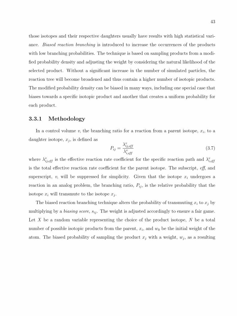
43

those isotopes and their respective daughters usually have results with high statistical vari-

ance. Biased reaction branching is introduced to increase the occurrences of the products

with low branching probabilities. The technique is based on sampling products from a modi-

fied probability density and adjusting the weight by considering the natural likelihood of the

selected product. Without a significant increase in the number of simulated particles, the

reaction tree will become broadened and thus contain a higher number of isotopic products.

The modified probability density can be biased in many ways, including one special case that

biases towards a specific isotopic product and another that creates a uniform probability for

each product.

3.3.1 Methodology

In a control volume v, the branching ratio for a reaction from a parent isotope, xi, to a

daughter isotope, xj, is defined as

Pij =λv

ij,eff

λvi,eff

(3.7)

where λvij,eff is the effective reaction rate coefficient for the specific reaction path and λv

i,eff

is the total effective reaction rate coefficient for the parent isotope. The subscript, eff, and

superscript, v, will be suppressed for simplicity. Given that the isotope xi undergoes a

reaction in an analog problem, the branching ratio, Pij, is the relative probability that the

isotope xi will transmute to the isotope xj.

The biased reaction branching technique alters the probability of transmuting xi to xj by

multiplying by a biasing score, sij. The weight is adjusted accordingly to ensure a fair game.

Let X be a random variable representing the choice of the product isotope, N be a total

number of possible isotopic products from the parent, xi, and w0 be the initial weight of the

atom. The biased probability of sampling the product xj with a weight, wj, as a resulting

44

product is given by

Bij = P (X = xj) =sijPij

N∑

k=1

sikPik

(3.8)

wj = w0Pij

Bij

(3.9)

It can easily be shown that the above formulations conserve the overall weight of Monte

Carlo particles by showing that the expected value of W is the same for the analog and

non-analog case.

E(W ) =N∑

k=1

wk · P (W = wk) =N∑

k=1

wk ·Bik

= w0

N∑

k=1

Pik

Bik

·Bik = w0

N∑

k=1

Pik = w0

Additionally, a fair game can be demonstrated by calculating the expected value of Wj. The

expectation of Wj corresponds to the branching ratio of the product, xj, multiplied by the

initial weight.

E(Wj) = wj · P (W = wj) = wj ·Bij = w0Pij

Bij

·Bij = w0Pij

Uniform reaction branching is a special case for biased reaction branching when sij is equal

to 1/Pij. Each product is sampled with equal biased probability, Bij = 1/N , and the weight

is multiplied by that product’s branching ratio multiplied by the total number of isotopic

products, N · Pij.

3.3.2 Test Problems

The inventories at shutdown following a 10-year steady state irradiation of 56Fe with a

uniform multi-group neutron flux of 5×1012 n/cm2s were calculated from three test problems

with different reaction sampling schemes. The first problem was a pure analog test problem

while the second problem had a uniform reaction branching technique applied and the third

problem was designed to improve the results of 53Mn. If 53Mn was present as a product, the

45

Category AnalogUniform

Reaction Branching

A number of products (n) 26 63

n < 5% statistical error 17 19

Mean statistical error 1.58% 1.84%

Mean relative difference 0.91% 2.13%

Table 3.2 Comparisons of different characteristic numbers of products between the analogresult and the results from a uniform reaction branching. The mean relative differences and

mean statistical errors are derived from those with statistical error less than 5% in eachcase.

biased reaction rates were calculated by increasing the 53Mn reaction rate by a factor of ten

and renormalizing the set of reaction rates. The test cases were simulated with 1010 Monte

Carlo particles and FENDL-2/A activation library and FENDL-2/D decay library were used

throughout. In addition, the results were compared with deterministic results from ALARA

using the truncation tolerance of 10−9.

3.3.3 Simulation Results

Table 3.2 compares the results between the analog problem and the non-analog test

problems. The analog problem produced 26 isotopes, including 56Fe. Of these, 17 have

statistical errors less than 5%. When compared to deterministic results, the average relative

difference of these seventeen isotopes was 0.91%. As expected, the test problem with uniform

reaction branching produced a much wider spectrum of isotopes than did the analog test

problem. Sixty-three isotopes were produced and 19 of these have statistical errors less than

5%. The average relative difference of these isotopes was found to be 2.13%. The variance

of some isotopes increased, in comparison to the analog case, because the uniform reaction

branching approach biases the solution away from those previously likely isotopes. In some

cases, this also resulted in larger deviations from the deterministic solution.

46

In particular, there were 15 isotopes from each case that had a statistical error less

than 5%. The analog problem had two isotopes that were not detected by the uniform

reaction branching problem. They were 59Co and 60Co because they occurred at least five

reactions from the initial isotope, 56Fe, and the uniform reaction branching widened and

implicitly shortened a reaction tree for the same number of Monte Carlo particles as the

analog case. Since the analog case allowed more histories to follow the reaction pathways

with high reaction rates, more histories were able to reach deep isotopes in the reaction tree.

On the other hand, the uniform reaction branching case produced four new isotopes with

statistical errors less than 5%. These isotopes(3H, 3He, 51V and 53Mn) were produced in the

analog case with extremely high statistical errors, as high as 44% for 3He. Those results

were statistically improved in the uniform reaction branching case because the technique

increased contributions from isotopes that were produced through reaction paths with low

probability. The light ions, 3H and 3He, benefitted most from the technique because they

were produced with low probability at many locations throughout the reaction tree.

In order to study the impact of biased reaction branching on a single isotope, the results

for 53Mn were studied. In the analog problem, the statistical error (precision) and the differ-

ence relative to the deterministic solution (accuracy) were 13.36% and 8.20%, respectively.

The substantial variance for this solution suggested that applying a variance reduction tech-

nique to improve precision would likely also lead to a better accuracy of the result. With

uniform reaction branching, both precision and accuracy improved, to 3.24% and 2.68% re-

spectively. However, the reaction branching biased specifically toward 53Mn did not perform

better than the uniform case as precision and accuracy became 4.92% and 7.84%.

The reaction chains of 53Mn from both cases were carefully examined to explain larger

errors of the biased reaction branching problem. The test problem with uniform reaction

branching produced sixty-seven reaction chains leading to the production of 53Mn while the

biased test problem generated only five such chains, all of which were included in the uniform

case. Based on a small number of reaction chains of 53Mn in the latter case, lack of accuracy

and precision in the 53Mn result was a direct consequence of the technique’s inability to

47

56Fe

55Fe55Mn

54Mn

53Mn

55Mn

54Mn

53Mn 54Mn 54Fe

53Mn 53Mn

53Mn

Figure 3.3 Most of the reaction chains leading to productions of 53Mn from auniform-branching problem, including all five chains from a biased-branching problem (◦),

are shown. The latter case fails to include most 53Mn’s production pathways and thusresults in much higher errors.

detect the 53Mn productions through reaction paths containing isotopes with relatively low

total effective reaction rate coefficients. Examples of those reaction chains are given below:

56Fe → 56Mn → 56Fe → 55Fe → 54Fe. → 53Fe → 53Mn,

56Fe → 54Mn → 53Mn → 52Mn → 53Mn → 54Mn → 53Mn,

56Fe → 54Mn → 53Mn → 54Mn → 53Mn → 54Mn → 53Mn,

56Fe → 54Mn → 55Mn → 55Cr → 55Mn → 54Mn → 53Mn,

56Fe → 55Mn → 56Mn → 56Fe → 55Fe → 54Mn → 53Mn,

56Fe → 54Mn → 53Mn → 52mMn → 52Mn → 52mMn → 52Mn → 53Mn.

Biasing only towards the target isotope fails to increase the probability of these relatively

rare precursor pathways, whereas uniform reaction branching raises the probability of rare

48

pathways and reduces the probability of likely pathways. Therefore, biasing a reaction tree

toward a particular isotope does not always maximize the accuracy and precision of its result

as the technique tends to underestimate significant contributions to the isotope’s inventory

from other reaction pathways. Defining a set of appropriate biasing scores that optimizes the

accuracy and precision of the isotope in question is a research challenge and might require

prior knowledge of the whole reaction tree and the extensive use of figure of merit that will

later be discussed.

3.4 Biased Source Sampling

Currently, the source is implemented by randomly sampling an isotopic identity and a

birth time from a probability density representing the isotopic compositions of the initial

material and from a time-dependent source strength, respectively. The simplest form is

the 0-D steady state source which is composed of a single isotope and the birth time is

characterized by a delta function. However, it is often not the case in a real world problem,

where the initial material can be composed of hundreds different isotopes. With analog

source sampling, isotopes with low concentrations give way to relatively small numbers of

sampled atom source, leading to statistically poor results for their respective products. The

biased source sampling technique is introduced to help increase the likelihood of sampling

the rare isotopic compositions. As a result, the technique reduces the statistical errors of

those products derived from rare initial isotopes. For example, the sampling mechanism can

be uniform among isotopic compositions or biased in favor of a specific isotope.

3.4.1 Methodology

The weight of the starting particle will be adjusted according to its real relative concen-

tration and biasing score. The implementation of this technique is strongly analogous to

the biased reaction branching technique with source compositions, atomic fractions and the

number of initial isotopes replacing reaction products, branching ratios and the number of

49

possible products, respectively. Formulations of biased source sampling hence are omitted

here.

3.4.2 Test Problems

The ability of biased source sampling to improve results of product isotopes transmuted

from rare initial isotopes was tested by studying the inventory at shutdown following a 10-

year steady state irradiation of natural iron(91.75% 56Fe, 5.85% 54Fe, 2.12% 57Fe and 0.28%

58Fe) with a uniform multi-group neutron flux of 5 × 1012 n/cm2s. Three test problems

with different sampling schemes were conducted. The first problem was a pure analog test

problem. The second one was a test problem with a uniform sampling technique and the

third one had its source biased toward 58Fe, which was the least abundant isotope in the

source. The test cases were simulated with 1010 Monte Carlo particles and FENDL-2/A

activation library and FENDL-2/D decay library were used. In addition, the results were

compared with deterministic results from ALARA, which solved the activation problems of

each initial source isotope individually to the specified truncation tolerance of 10−9.

3.4.3 Simulation Results

The test problem with uniform source sampling technique applied was expected to equally

distribute initial Monte Carlo particles among isotopic source compositions. Isotopes with

relatively high concentrations would be chosen less frequently; therefore, the statistical errors

of their respective products would be higher than results from an analog problem. At the

same time, the occurrences of the rare source isotopes would be more favorable and would

yield results with lower statistical errors than those from an analog problem. As a result,

the overall variation in statistical errors of isotopic products would be smaller. The uniform

source sampling problem produced 41 products and 27 of those had statistical errors less

than 5% while the analog problem yielded 35 products with 26 products having statistical

errors less than 5%. Figure 3.4 compared the results from both problems to the deterministic

results by showing the relative differences of results with statistical errors less than 5% as a

50

10-10

10 -8

10 -6

10 -4

10 -2

100

0.001

0.01

0.1

1

10

100

Deterministic Result

Relative Difference (%)

Analog SamplingUniform Sampling

Figure 3.4 Relative Differences between Monte Carlo results with statistical errors lessthan 5% and deterministic results as a function of the deterministic result.

function of the deterministic results. Slight improvements on both accuracy and precision

were achieved as the average relative differences were found to be 0.7582% and 0.9646%

and the statistical errors of the averages were 1.32% and 1.79% for uniform source sampling

results and analog results, respectively.

It is important to note that uniform source sampling is simply equivalent to performing

calculations on individual isotopic compositions independently and weight-averaging all of

the results, according to their initial source concentrations. The technique is only useful in

a problem where there is no target isotope or the overall statistical improvement is desired.

The last test problem was designed to evaluate the capabilities of biased source sampling.

It was aimed to increase the sampling frequency of the least abundant isotope, 58Fe, and thus

reduce statistical errors of its products. 59Fe was a direct product of 58Fe and had a statistical

error of 1.27% from an analog problem with 1010 particles. The test problem was set up

such that 58Fe was likely to be sampled three times as often as the other isotopes combined.

As a result, the statistical error of 59Fe was reduced to 0.08% with the same number of

simulated particles. However, the statistical error of about 1.20% could be achieved in the

biased problem using only 5 × 107 particles. In this case, the computing time was reduced

by about two orders of magnitude; however, the improvement of 59Fe’s result came at the

expense of the other isotopic results’ statistical qualities.

51

3.5 Reaction Path Splitting

As mentioned earlier, a new isotopic identity for a current atom undergoing a reaction is

obtained from randomly sampling a probability density function made of a list of possible

daughters and a corresponding list of effective reaction rate coefficients. This sampling

mechanism results in fewer histories for those daughters with smaller effective reaction rate

coefficients. Even though Biased Reaction Branching could be used to increase frequencies

of such histories, it could essentially create another statistical problem by sampling fewer

histories of unbiased isotopes. Moreover, it could also introduce a weight factor substantially

larger than one. Reaction Path Splitting is implemented to allow a simulation to track

down every possible reaction pathway by splitting the atom having a reaction into as many

new atoms as the number of pathways and adjusting their weights relatively according to

their actual effective reaction rate coefficients. While the technique might still produce

large variations in weight factors, it would ensure that all histories of reaction products are

followed, regardless of the effective reaction rate coefficients.

3.5.1 Methodology

At a reaction point of a parent isotope, xi, the atom will be split into x1, x2, x3, ..., xk,

where k is the total number of possible products. A weight, wj, of each newly created atom

must be adjusted, based on the initial weight, w0 and the branching ratio, Pij, which was

previously defined in Equation (3.7).

wj = w0 · Pij j = 1, 2, 3, ..., k (3.10)

It can easily be shown that the overall weight is conserved after a splitting process.

k∑j=1

wj =k∑

j=1

(w0 · Pij)

= w0

k∑j=1

Pij

= w0

52

3.5.2 Test Problem

The isotopic inventories following a 10-year steady state irradiation of 56Fe with a uniform

multi-group neutron flux of 5 × 1012 n/cm2s were obtained from a test problem in which

Reaction Path Splitting was applied. FENDL-2/A activation library and FENDL-2/D decay

library were used in the simulation.

3.5.3 Simulation Results

The test problem with 15000 simulated particles and a computing time of 524 seconds

produced 82 isotopes while the analog problem with a comparable computing time produced

22 isotopes. Table 3.3 quantitatively compares results between the test problem and the

analog problem. The test problem detected isotope productions ranging from 9.7780×10−54

to 9.8299 × 10−1 with statistical errors of 100% and 0.8227%, respectively. For the analog

problem to have a chance to detect this minute production, the problem would require at

least 1.0227×1053 particles or 4.0908×1055 if a statistical error of less than 5% were desired,

according to Equation (2.11). Moreover, most isotopes in the test problem were tallied

with statistical errors above 10% whereas there were only five such isotopes in the analog

case. Based on this metric, the analog case seemed to reach its saturation limit in terms

of precision improvement. This suggested that increasing the number of simulated particles

in the analog case would not improve the overall precision as much as it would in the test

problem. The reaction path splitting technique clearly improved the detection limit without

spending too much computational effort on the problem while the technique also ensured

that every reaction pathway was followed in an event of the atom having a reaction.

To evaluate the validity of the reaction path splitting technique, only statistically reliable

results of nine isotopes were compared to deterministic results from ALARA. Relative dif-

ferences and statistical errors were plotted as a function of deterministic results as shown in

Figure 3.6. In all cases, the relative differences were less than 5% and, more importantly,

lower than statistical errors which indicated that the discrepancies were likely dominated

53

0 10 20 30 40 50 60 70 80 90 1000

5

10

15

20

25

Interval (Statistical error %)

Number of isotopic products

Figure 3.5 A histogram representing numbers of products from a reaction path splittingtest problem characterized by statistical errors

10-6

10 -4

10 -2

100

10 -1

100

101

Deterministic Result

Relative Difference (%)

Relative ErrorStatistical Error

4.60

0.13

Figure 3.6 Relative Differences between Monte Carlo results with statistical errors lessthan 10% and deterministic results as a function of the deterministic result. Dash-dot lines

connect relative differences to their corresponding statistical errors.

54

Category AnalogReaction

Path Splitting

NPS 250M 15k

Computing Time (s) 546 524

A number of products (n) 22 82

n < 10% stat. error 14 9

10% < n < 20% stat. error 0 5

20% < n < 30% stat. error 2 2

30% < n < 40% stat. error 2 2

40% < n < 50% stat. error 2 10

50% < n < 60% stat. error 0 11

60% < n < 70% stat. error 0 12

70% < n < 80% stat. error 1 5

80% < n < 90% stat. error 0 5

90% < n < 100% stat. error 1 21

Mean statistical error 2.11% 5.58%

Mean relative difference 1.44% 1.40%

Table 3.3 Quantitative comparisons of different characteristic numbers of productsbetween the analog result and the results from a reaction path splitting. The mean relativedifferences and mean statistical errors are derived from those with statistical error less than

10% in each case.

55

by statistical variations in the simulation. This relationship suggested that smaller relative

differences could be obtained from the simulation with improved statistics.

3.6 Weight Window

The use of variance reduction techniques can increase the number of desired histories but

often introduce large fluctuations in the weights of the particles following these histories.

The latter effect somewhat negates the purpose of applying variance reduction techniques as

these fluctuations usually contribute to larger variances of the results.

Traditionally in Monte Carlo transport, a weight-window technique has been employed

to control the weight variations in the non-analog simulation [13]. A weight window, or for

short, a window, is defined for each spatial region and energy range and characterized by the

upper and lower bound on a particle’s weight. If a particle’s weight is below the lower bound,

Russian roulette is applied and the particle’s weight is increased to be within the window

or the particle is terminated. On the other hand, if the particle’s weight is higher than the

upper bound, the particle will be split such that the weights of new particles are within the

window. Due to a strong analogy to Monte Carlo transport, Monte Carlo inventory analysis

might be able to take full advantage of the well-established concept of window. This chapter

introduces the application of window in the current work.

3.6.1 Development Scope

The development is focused on the implementation of the time-dependent window analo-

gous to the space-dependent window in Monte Carlo transport. The time-dependent window

in Monte Carlo inventory is strictly defined as a function of control volumes. It is indepen-

dent of isotopic identities. This type of window is the simplest definition of a weight window

which serves as the initial stage of validating the benefits of weight window in Monte Carlo

inventory and to provide the concrete stepping stone for future extensions, for example, an

automated weight-window generator or a time-isotope dependent weight window.

56

3.6.2 Methodology

A weight window in any control volume is characteristically defined with a lower-bound(wl),

upper-bound(wu) and target(wt) weight. A primary task of weight window is to split or

roulette a particle when its weight, w, is higher than the upper-bound weight or less than

the lower-bound weight without unbiasedly affecting the simulation. In both cases, the num-

ber of newly created particles, n, is given by the combined Russian rouletting & splitting

scheme [17]:

n = b w

wt

+ ξc, ξ ∈ Unif [0, 1). (3.11)

The initial particle is discarded and replaced with n particles, each with the same weight

of wt. It can be shown that the overall weight is conserved after the splitting or rouletting

processes by calculating the expected weight of the particles.

E(W ) = E(wtn) = wt · E(n) (3.12)

The expected value of n can be calculated with aid from the following expression derived

from Equation (3.11).

n =

b w

wtc if ξ ≤ 1− ( w

wt− b w

wtc)

b wwtc+ 1 if ξ > 1− ( w

wt− b w

wtc)

(3.13)

57

Hence,

E(n) =k∑

i=1

ni · P (n = ni)

= b w

wt

c · P (n = b w

wt

c) + (b w

wt

c+ 1) · P (n = (b w

wt

c+ 1))

= b w

wt

c · (1− (w

wt

− b w

wt

c)) + (b w

wt

c+ 1) · ( w

wt

− b w

wt

c)

= b w

wt

c − b w

wt

c w

wt

+ b w

wt

cb w

wt

c+ b w

wt

c w

wt

− b w

wt

cb w

wt

c+w

wt

− b w

wt

c

=w

wt

(3.14)

∴ E(W ) = wt · w

wt

= w (3.15)

3.6.3 Testing

After the fundamental concept of the window is established, the implementation of the

window is tested by applying a number of different weight windows in a simulation expected

to have a broad range of particle weights and comparing these results to the deterministic

result. The simulation is based on isotopic inventories following a 10-year steady state

irradiation of 56Fe with a uniform multi-group neutron flux of 5 × 1012 n/cm2s. The forced

reaction technique with a parameter of 1 and the reaction path splitting technique are applied

in the simulation. Five weight windows with different lower bounds are used in the simulation

to construct five testing problems. The upper-bound and target weight of all windows are

2 and 10−2, respectively, while the lower-bound weights are 10−10, 10−20, 10−30, 10−40 and

10−50. All five testing problems run with 105 NPS.

Some characteristics of the results are summarized in Table 3.4. As expected, the test

problems with wider weight windows produce more products and smaller detection limits

than the test problems with narrower windows. The detection limit in each case is slightly

lower than its respective lower-bound weight because any simulated particles with weight less

than the lower bound is either terminated or promoted by increasing its weight to be within

the window. As a result, the smallest possible isotopic result in a single tally bin is equal to a

58

ratio of the lower bound and NPS where only one Monte Carlo particle with the same isotopic

identity and the lower bound weight reaches that tally bin in the simulation. Improvements

of detection limits and numbers of products come with the expense of computing times and

statistical errors. The computing time increases dramatically with increasing the width of

the window. This is due to a higher number of Monte Carlo particles being tracked by the

simulation. The root-mean-squared relative error also increases with increasing the width

of the window, reflecting a larger variance from a higher variation of particles’ weights. To

verify the validity of the weight window implementation, the results with relative errors

less than 10% are compared to the deterministic results from ALARA. They are in good

agreements as the average relative differences range from 1.80% to 3.85% and are less than

their relative errors in all cases. This relationship suggests that smaller relative differences

can be achieved by means of improving statistics, i.e. increasing NPS.

After the implementation of the window is validated, the next challenging task is to

select appropriate values of window parameters: lower-bound weight and window width.

Defining the latter implies the value of an upper-bound weight. A target weight would be

defined within the window. Strong analogy between MC inventory analysis and neutron

transport suggests that existing selection process of weight window parameters in neutron

transport could be readily applicable to MC inventory. Thus, extensive literature review

of this topic has been conduct for possible solutions. Recently, an approach of using a

forward deterministic solution to compute weight window for a deep-penetration problem

in slab geometry has been studied [18]. Even though this technique greatly increases the

efficiency of Monte Carlo simulations, its applicability is likely limited to problems with

simple geometry. When the geometry is more complicated, there might not be a theoretical

analysis for the optimal width and the selection of the width is empirical.

The default upper bound in MCNP and its descendants is five times the lower bound,

although it is observed that different window widths made slight difference to the efficiency

of the simulation [19]. In most cases, the weight window is generally quite insensitive to

the window width and there is a broad range of window parameters in which the weight

59

CategoryLower-bound weight

10−10 10−20 10−30 10−40 10−50

Number of products 23 40 61 84 94

Detection limit2.99e-14 1.37e-22 3.95e-34 3.43e-44 3.87e-53

(per initial source)

Computing time9.05 16.22 89.15 1126.48 14978.90

(seconds)

R.M.S. relative error34.47 54.90 59.93 61.00 68.87

(percent)

Only results with relative errors less than 10% are considered.

Avg. relative difference2.13 1.80 3.16 3.85 2.78

(percent)

R.M.S. relative error3.83 4.11 4.15 4.08 4.02

(percent)

Table 3.4 Summary of characteristics of the results from the simulations with differentdefinitions of weight window.

60

window perform equally well [20]. An importance generator, later known as a weight window

generator, has been developed to efficiently set the window parameters for energy-dependent

problems [20]. Essentially, it is a bookkeeping algorithm which empirically estimates the

importance function of a cell for subsequent calculations [14].

In conclusion, an analytic method to determine the optimal parameters for the weight

window in general inventory problems may not exist. In addition, the effect of different

weight window on computational efficiency is undetermined. For these reasons, along with

the goal of providing a more user-friendly environment, a weight window generator and

time-isotope dependent window would be the subjects of interest for future development.

Borrowing from MCNP, one approach is to model the weight window generator following

the forward-adjoint generator [14]. Note that when defining parameters for the window, a

precaution must be taken as too narrow window might terminate or split too many particles

and too wide window might not improve enough efficiency.

3.7 Delta Tracking

One of the most important issues in many activation problems is accounting for pulsed

or intermittent operation of the neutron source. While exact treatment of this pulsing is not

always required [21], some cases do require it for accurate determination of the activation

products. The current methodology could be used to simulate a pulsed neutron source on

a non-flowing material by using the loop and flow capabilities. One control volume would

represent the irradiation time (on-time) and another would represent the dwell time (off-time)

between pulses. However, there are two potential problems with such an implementation.

First, for systems with high pulse frequencies and operation times of many years, this might

result in excessive computation as an MC atom passes through the loop many times without

any reactions. More importantly, however, is the situation where flowing material, moving

through the system with one characteristic frequency, is subjected to a pulsed neutron source

of another characteristic frequency. This can result in a complex and potentially long series

of control volumes before it repeats. Furthermore, if the physical flowing system is modeled

61

by a complex loop flow, there may be no definable characteristic flow frequency and it would

be impossible to define a set of control volumes that would represent all atoms.

The solution is to handle the time-varying nature of the neutron flux in a different

manner within the control volumes rather than as a defining aspect of the control volumes.

At least two approaches are being considered for this, one that relates to the concept of delta

tracking [17] and one that explores the validity of various pulse approximations.

The delta tracking technique is considered to be an interesting approach and is well

established in neutron transport. The implementation of delta tracking for MC inventory

analysis will follow a close analogy to MC transport.

3.7.1 Methodology

The delta tracking technique is applied in a control volume with a pulsing schedule. In

order to demonstrate this technique, the pulsing schedule is limited to include only pulsing

time, tp, and dwelling time, td, between two pulses. These two characteristic times must

be defined in addition to other quantities necessary for a complete definition of a pulsing

control volume. The effective reaction rate coefficient during the pulse, λp, can be calculated

from a prescribed neutron spectrum in the control volume while the effective reaction rate

coefficient during a delay, λd, is simply equal to a decay constant.

The underlying methodology of delta tracking is to give a simulated atom a constant

effective reaction rate coefficient, λ′, which is given by

λ′ = λT (t) + λδ(t), λ′ ≥ λT (t), λδ(t) ≥ 0 for all t > 0, (3.16)

where λT (t) is a true effective reaction rate coefficient and λδ(t) is a fictitious effective

reaction rate coefficient, representing ”pseudo-reaction” events.

A potential reaction time is randomly sampled based on λ′. This can easily be done using

the following expression.

t′ = − ln ξ

λ′, where ξ ∈ Unif[0, 1) (3.17)

62

Based on durations of pulsing and dwelling time, an effective reaction rate coefficient at

this potential reaction time, λT (t′), can be randomly determined.

λT (t′) =

λp if η ≤ tptp+td

, where η ∈ Unif[0, 1)

λd Otherwise

(3.18)

Whether the simulated atom undergoes a reaction at this point in time entirely depends

on a rejection sampling method, which is based on a ratio of λδ(t′) and λ′. With probability

λδ(t′)λ′ , this potential reaction time is rejected. Otherwise, the atom undergoes a reaction, the

daughter will be randomly sampled from a set of products corresponding to a region which

is previously determined from Equation 3.18.

This procedure is repeated until the atom exits the control volume or its history is

terminated.

Note that the delta tracking technique should be used in a problem where a pulsing

frequency is so high that a duration of each pulse is short compared to the residence time

of the control volume. The technique can produce statistically invalid results if it is used in

a problem with very long pulses and delays. Equation 3.18 would yield the same expected

mean from two problems with drastically different frequencies but same total on-times and

off-times.

It can be shown that the delta tracking technique is an unbiased sampling method. The

following proof is recast from Monte Carlo Fundamentals by Brown and Sutton [17].

Let P (u) be the total probability of traveling through a time, u, without a real reaction

and P (u|n) be the probability of having exactly n pseudo-reactions during this time, u.

63

Therefore, P (u) =∞∑

n=0

P (u|n).

P (u|0) = 1−u∫

0

λ′e−λ′tdt

P (u|0) = e−λ′u (3.19)

P (u|1) =

u∫

0

P (t|0)P (u− t|0)λδ(t)dt =

u∫

0

e−λ′te−λ′(u−t)λδ(t)dt

= e−λ′u

u∫

0

λδ(t)dt = e−λ′uΘδ(u) ∵ Θδ(u) =

u∫

0

λδ(t)dt (3.20)

P (u|2) =

u∫

0

P (t|1)P (u− t|0)λδ(t)dt =

u∫

0

Θδ(t)e−λ′te−λ′(u−t)λδ(t)dt

= e−λ′u

u∫

0

Θδ(t)λδ(t)dt =[Θδ(u)]2

2e−λ′u (3.21)

P (u|n) =

u∫

0

P (t|n− 1)λδ(t)P (u− t|0)dt =[Θδ(u)]n

n!e−λ′u for all n ≥ 1 (3.22)

P (u) =∞∑

n=0

P (u|n) =∞∑

n=0

[Θδ(u)]n

n!e−λ′u

P (u) = eΘδ(u)e−λ′u = e(Θδ(u)−λ′u)

P (u) = exp

u∫

0

λδ(t)dt−u∫

0

λ′dt

= exp

−

u∫

0

λT (t)dt

(3.23)

Equation 3.23 agrees with the interpretation of the total effective reaction rate coefficient in

the analog sampling.

3.7.2 Test Problems

The inventories at shutdown following a 10-year pulsing irradiation of 56Fe with a uniform

multi-group neutron flux of 5 × 1012 n/cm2s were calculated from two test problems with

different schemes to model the same pulsing schedule. The pulsing time and dwelling time

between pulses were defined to be three and two minutes, respectively. The first test problem

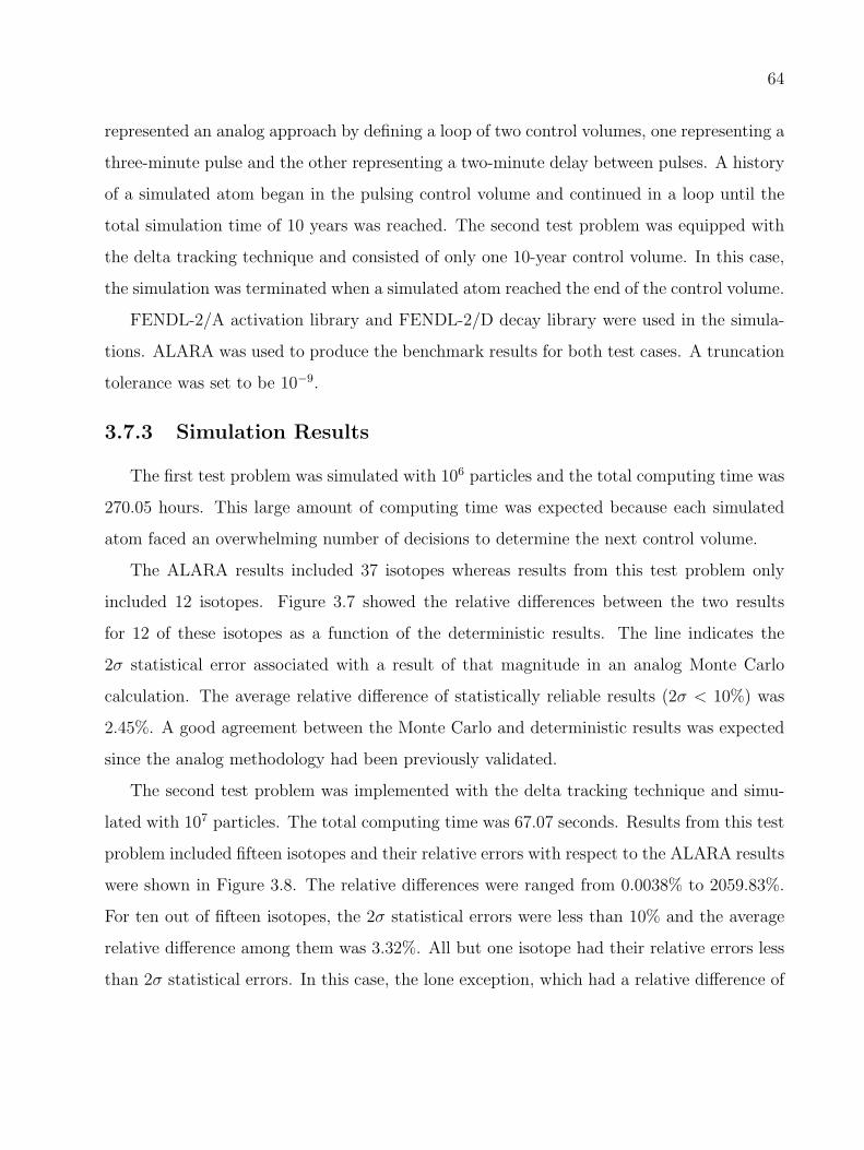
64

represented an analog approach by defining a loop of two control volumes, one representing a

three-minute pulse and the other representing a two-minute delay between pulses. A history

of a simulated atom began in the pulsing control volume and continued in a loop until the

total simulation time of 10 years was reached. The second test problem was equipped with

the delta tracking technique and consisted of only one 10-year control volume. In this case,

the simulation was terminated when a simulated atom reached the end of the control volume.

FENDL-2/A activation library and FENDL-2/D decay library were used in the simula-

tions. ALARA was used to produce the benchmark results for both test cases. A truncation

tolerance was set to be 10−9.

3.7.3 Simulation Results

The first test problem was simulated with 106 particles and the total computing time was

270.05 hours. This large amount of computing time was expected because each simulated

atom faced an overwhelming number of decisions to determine the next control volume.

The ALARA results included 37 isotopes whereas results from this test problem only

included 12 isotopes. Figure 3.7 showed the relative differences between the two results

for 12 of these isotopes as a function of the deterministic results. The line indicates the

2σ statistical error associated with a result of that magnitude in an analog Monte Carlo

calculation. The average relative difference of statistically reliable results (2σ < 10%) was

2.45%. A good agreement between the Monte Carlo and deterministic results was expected

since the analog methodology had been previously validated.

The second test problem was implemented with the delta tracking technique and simu-

lated with 107 particles. The total computing time was 67.07 seconds. Results from this test

problem included fifteen isotopes and their relative errors with respect to the ALARA results

were shown in Figure 3.8. The relative differences were ranged from 0.0038% to 2059.83%.

For ten out of fifteen isotopes, the 2σ statistical errors were less than 10% and the average

relative difference among them was 3.32%. All but one isotope had their relative errors less

than 2σ statistical errors. In this case, the lone exception, which had a relative difference of

65

10-6

10 -4

10 -2

100

10 -3

10 -2

10 -1

100

101

102

103

Deterministic Result

Relative Difference (%) 2σ Statistical Error(%)

Figure 3.7 Relative differences (%) between deterministic results and Monte Carlo resultsfrom the test problem with the exact pulsing schedule were plotted as a function of

deterministic results. NPS = 106.

10-10

10 -8

10 -6

10 -4

10 -2

100

10 -3

10 -2

10 -1

100

101

102

103

104

Deterministic Result

Relative Difference (%)

2σ Statistical Error(%)

Figure 3.8 Relative differences (%) between deterministic results and Monte Carlo resultsfrom the test problem with the delta tracking technique were plotted as a function of

deterministic results. NPS = 107.

66

2059.83%, occurred in a region where a statistical error was too high that this result would

be disregarded.

Having statistical errors higher than relative differences suggested that the differences

were likely dominated by the statistical variations in the results and smaller differences

could result from improved statistics of the simulation. More importantly, this behavior

verified that the delta tracking technique had been successfully implemented.

Computing times of both test problems were compared to evaluate their efficiency to

model the pulsing schedule. The first test problem required 270.05 hours while the second

test problem with the delta tracking technique only needed 67.07 seconds to perform the

same physical task. In addition to a significant reduction in a computing time, the second

problem was able to simulated ten times more particles than the first problem. Clearly,

employing the delta tracking was a better alternative to using a loop of two control volumes

representing a pulse and a delay as evident by a substantial difference of computing times

by several orders of magnitude.

3.8 Summary

In addition to simply increasing the number of simulated particles, variance reduction

techniques are alternative methods to improve the precision of the results of isotopic in-

ventory problems. To this point, six variance reduction techniques: forced reaction, biased

source sampling, biased reaction branching, reaction path splitting, weight window and delta

tracking have been studied and successfully implemented. With variance reduction tech-

niques applied , precision, accuracy and efficiency of the problem have been tremendously

improved. However, using only one technique at a time might not produce the most efficient

modeling scheme in most situations. The combination of several techniques and appropri-

ate parameter inputs are recommended. As an example, forced reaction and reaction path

splitting would be used together to both deepen and broaden a reaction tree. Nonetheless,

finding suitable parameters for each technique that yields optimal performance is quite a

challenging task. Furthermore, use of variance reduction techniques can be less efficient

67

than the analog simulation because the statistical improvement might not be high enough

to surplus the increase in computing time per each Monte Carlo history. A figure of merit

was then introduced as a tool to evaluate the efficiencies of different modeling schemes on

the same physical problem, leading to the optimal variance reduction parameters.

68

Chapter 4

Figures of Merit

Monte Carlo isotopic inventory analysis is directly analogous in many ways to Monte

Carlo neutral particle radiation transport; instead of neutral particles traveling through 3-

dimensional space and having interactions with the underlying materials that change their

energy, inventory analysis simulates atoms moving through (1-D) time and having interac-

tions with the underlying neutron flux that change their isotopic identity. After a description

of the fundamental Monte Carlo methodology, including some basic variance reduction meth-

ods, and of the motivation and goals for the development of a figure of merit, this chapter

will explore a number of possible figures of merit and discuss their applicability to different

types of simulations.

4.1 Introduction and Importance of Figure of Merit

Even though the variance reduction techniques have tremendously reduced the statistical

error and increased the spectrum of isotopes generated in the Monte Carlo simulation, they

also increase the computer time spent calculating each history and thus are not guaranteed

to optimize the computing resource for such calculations. That is, in some cases it may be

more efficient to simply simulate more histories than use a variance reduction technique.

A figure of merit (FOM) is introduced to monitor the efficiency of the Monte Carlo code

as different variance reduction techniques are attempted on the same problem [11]. FOMs

representing relative efficiencies from biased and unbiased runs of the same physical problem

can be calculated and compared quantitatively, assisting a user in determining the optimal

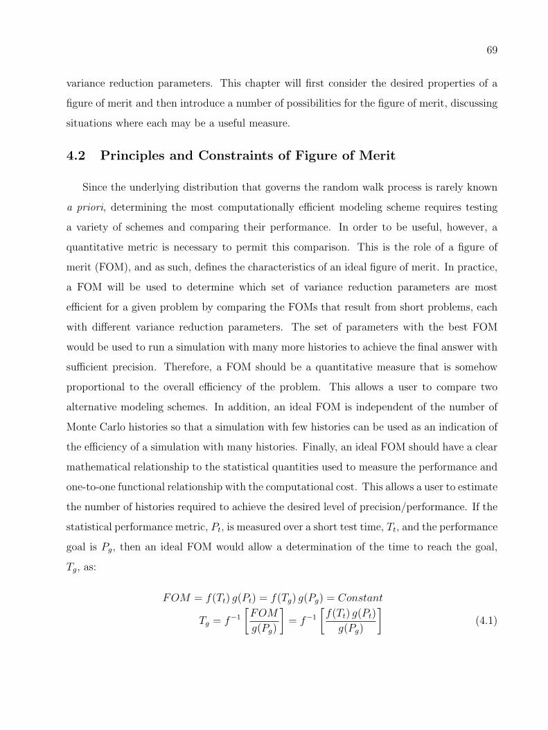
69

variance reduction parameters. This chapter will first consider the desired properties of a

figure of merit and then introduce a number of possibilities for the figure of merit, discussing

situations where each may be a useful measure.

4.2 Principles and Constraints of Figure of Merit

Since the underlying distribution that governs the random walk process is rarely known

a priori, determining the most computationally efficient modeling scheme requires testing

a variety of schemes and comparing their performance. In order to be useful, however, a

quantitative metric is necessary to permit this comparison. This is the role of a figure of

merit (FOM), and as such, defines the characteristics of an ideal figure of merit. In practice,

a FOM will be used to determine which set of variance reduction parameters are most

efficient for a given problem by comparing the FOMs that result from short problems, each

with different variance reduction parameters. The set of parameters with the best FOM

would be used to run a simulation with many more histories to achieve the final answer with

sufficient precision. Therefore, a FOM should be a quantitative measure that is somehow

proportional to the overall efficiency of the problem. This allows a user to compare two

alternative modeling schemes. In addition, an ideal FOM is independent of the number of

Monte Carlo histories so that a simulation with few histories can be used as an indication of

the efficiency of a simulation with many histories. Finally, an ideal FOM should have a clear

mathematical relationship to the statistical quantities used to measure the performance and

one-to-one functional relationship with the computational cost. This allows a user to estimate

the number of histories required to achieve the desired level of precision/performance. If the

statistical performance metric, Pt, is measured over a short test time, Tt, and the performance

goal is Pg, then an ideal FOM would allow a determination of the time to reach the goal,

Tg, as:

FOM = f(Tt) g(Pt) = f(Tg) g(Pg) = Constant

Tg = f−1

[FOM

g(Pg)

]= f−1

[f(Tt) g(Pt)

g(Pg)

](4.1)

70

In summary, an ideal figure of merit has the following characteristics:

• quantitative measure of statistical performance,

• independent of number of Monte Carlo histories, and

• a one-to-one function of the computational cost.

While previous work on determining the efficiency of simulations provides a rigorous

decision-theoretic framework evaluating and possibly determining the efficiency of simula-

tions [22], this work takes an approach based more directly on the desired physical outcomes

of the simulation. Future work can be carried out to reconcile the efficiency measures devel-

oped here with the mathematical development in [22].

The following sections will consider a variety of potential FOMs, both for these charac-

teristics and for other ways that they provide information about the problems performance.

Test Problem

The performance of each FOM was tested by calculating the proposed FOM at shutdown

following a 10-year steady state irradiation of 56Fe with a uniform multi-group neutron flux

of 5× 1012 n/cm2 s. In all cases the FENDL-2/A activation library and FENDL-2/D decay

library were used. The results for the analog case were compared to non-analog cases with

forced reaction parameters of 1, 2, 3, 5, and 8. The forced reaction parameter indicates the

number of times an isotope will be forced to undergo a reaction within the 10-year irradiation

period. The FOM was calculated for each case as a function of time, in increments of 1000

seconds of computer time.

4.3 Development of Figures of Merit

Based on the above characteristics, developing a Figure of Merit requires first choosing

a statistical performance metric and then examining its relationship to the computational

cost to arrive at a formulation that is independent of the number of histories. A variety

71

of statistical performance metrics are available and they form the basis for distinguishing

among the four FOM formulations proposed in this section. The behavior of the specific

statistical performance metric will be considered first and then its usefulness in formulating

a FOM will be addressed.

4.3.1 Statistical Error of Single Result (1 / R2T)

The strong analogy between this methodology and Monte Carlo neutral particle transport

results in an obvious suggestion for a FOM based on the statistical error of the result. In

this case, the statistical performance metric is the square of the relative statistical error,

R, which is known to vary inversely with the number of Monte Carlo particles and hence

inversely with the computational cost, T. Thus, a FOM based on this metric is

FOM =1

R2T(4.2)

Implicitly, this metric/FOM is based on the relative error of a single tally result, or single

tally bin. Consequently, optimizing this FOM amounts to optimizing the results for only that

tally bin and only improves the whole problem to the extent that the tally bin in question

represents the rest of the problem. In the current Monte Carlo inventory implementation, the

tally bins are based on time (analogous to space in Monte Carlo transport) and/or isotopic

identity (analogous to energy in Monte Carlo transport). Using this FOM, therefore, requires

the choice of a specific time and isotopic identity.

It is important at this stage to point out a distinct difference between the inventory

analysis and the neutral particle transport methods. The energy domain of neutral particle

transport is a continuous dimension where two different energies have a clear physically

meaningful relationship to each other. This often allows a single energy bin (or the total over

all energy bins) to be representative of the results over the entire energy domain. The isotopic

identity domain is discrete and two isotopic identities may not have any clear relationship to

each other. Hence a single isotopic identity bin is unlikely to be representative of many other

isotopic identities, and rarely representative of the whole problem. This FOM is therefore

only valuable in optimizing the modeling scheme for a particular isotope, i. For this study,

72

the inventories at the end of a 10-year irradiation period were used to calculate while the

FOMs, comparing results for a variety of specific represented isotopes, still remained in

question.

Since R2 is inversely proportional to T and T is directly proportional to the number

of histories, FOM should be constant with respect to the number of histories (allowing for

statistical fluctuations at very small numbers of histories). Three isotopes from the test

problem, 56Fe, 54Cr and 59Co, with different relative expected end-of-problem inventories of

9.82×10−1, 3.10×10−5 and 4.29×10−7, were chosen to be isotopes in question. The behaviors

of the three resulting FOM values are shown in Figure 4.1(a-c), demonstrating the effects

of increasing the forced reaction parameter. The FOM for all three isotopes are constant as

expected. For 56Fe, this FOM suggests that the analog scheme is much more efficient than

forced reactions technique. This agrees with the physical nature of the problem; because 56Fe

is the initial isotope, forcing a reaction will only reduce the variance of the products in the

reaction chain, but will make each history have a higher computational cost. On the other

hand, both 54Cr and 59Co are produced predominantly from the third reaction from 56Fe

and the forced reaction technique with parameter of 3 improves the likelihood of producing

these isotopes with the minimum increase in the computational cost of each history. This

FOM confirms that this is the optimal choice for these isotopes.

Finally, this FOM can be used to estimate a computing time to achieve a target error for

the isotope in question:

Tg =1

R2g · FOM

=R2

t Tt

R2g

, (4.3)

as described in Equation (4.1). This FOM has all of the characteristics of an ideal FOM

defined above, but the performance metric itself is only useful in special circumstances. Since

the important isotopes are not always known a priori and one isotope’s results are rarely

indicative of another’s, other potential performance metrics and FOMs will be explored.

73

0 5 10

0

1

2

3

4

5

6

7

8

[× 104 s]

1 / R2 T [

× 100]

Analog

FR1

FR2

FR3

FR5

FR8

59Co

c)

0 5 100

0.5

1

1.5

2

Computational Time[× 104 s]

1 / R2 T [

× 105]

Analog

FR1

FR2

FR3

FR5

FR8

56Fe

a)

Computational Time

0 5 100

0.5

1

1.5

2

2.5

Computational Time [× 104 s]

1 / R2 T [

× 100]

Analog

FR1

FR2

FR3

FR5

FR8

54Cr

b)

Figure 4.1 Traditional figure of merit based on relative error, shown for three differentisotopes as a function of time and for different forced reaction(FR) parameters: a)56Fe

b)54Cr c)59Co.

74

0 2 4 6 8 10

0

5

10

15

20

25

Computational Time [× 104 s]

N1%

analog 1 2 3 5 8

Figure 4.2 Number of qualified isotopes with relative error less than 1%. Theperformances of the test problem with different FR parameters are compared using the

number of qualified isotope metric.

4.3.2 Number of Qualified Isotopes (Nk)

Another performance metric for the Monte Carlo inventory method is the number of

isotopes produced by a given set of modeling parameters. If the statistical error for a

particular isotope is too high; however, it should be disregarded. The number of qualified

isotopes, Nk, is defined as the number of isotopes that have relative errors less than k

percent. This quantity is the simplest measurement of the performance for a given modeling

technique.

Figure 4.2 shows the results for this performance metric for a k of 1% and for a variety of

modeling schemes represented by the forced reaction parameter. For very short run times, all

cases produce approximately the same number of qualified isotopes. As the computing time

progresses, Figure 4.2 clearly shows that forced reaction problems with higher parameter(3,

5 and 8) perform similarly, but better than problems with lower forced reaction parameters.

Increasing the number of Monte Carlo particles and thus computing time would decrease

relative errors of all isotopes. Consequently, more isotopes would be counted as qualified

isotopes. This performance measure is expected to have this step behavior until the max-

imum number of isotopes is qualified, with the more efficient variance reduction schemes

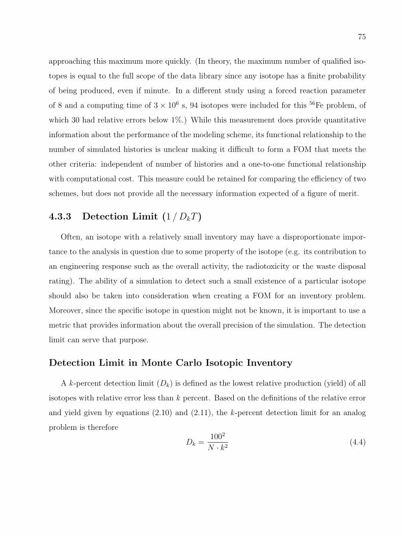
75

approaching this maximum more quickly. (In theory, the maximum number of qualified iso-

topes is equal to the full scope of the data library since any isotope has a finite probability

of being produced, even if minute. In a different study using a forced reaction parameter

of 8 and a computing time of 3 × 106 s, 94 isotopes were included for this 56Fe problem, of

which 30 had relative errors below 1%.) While this measurement does provide quantitative

information about the performance of the modeling scheme, its functional relationship to the

number of simulated histories is unclear making it difficult to form a FOM that meets the

other criteria: independent of number of histories and a one-to-one functional relationship

with computational cost. This measure could be retained for comparing the efficiency of two

schemes, but does not provide all the necessary information expected of a figure of merit.

4.3.3 Detection Limit (1 /DkT )

Often, an isotope with a relatively small inventory may have a disproportionate impor-

tance to the analysis in question due to some property of the isotope (e.g. its contribution to

an engineering response such as the overall activity, the radiotoxicity or the waste disposal

rating). The ability of a simulation to detect such a small existence of a particular isotope

should also be taken into consideration when creating a FOM for an inventory problem.

Moreover, since the specific isotope in question might not be known, it is important to use a

metric that provides information about the overall precision of the simulation. The detection

limit can serve that purpose.

Detection Limit in Monte Carlo Isotopic Inventory

A k -percent detection limit (Dk) is defined as the lowest relative production (yield) of all

isotopes with relative error less than k percent. Based on the definitions of the relative error

and yield given by equations (2.10) and (2.11), the k -percent detection limit for an analog

problem is therefore

Dk =1002

N · k2(4.4)

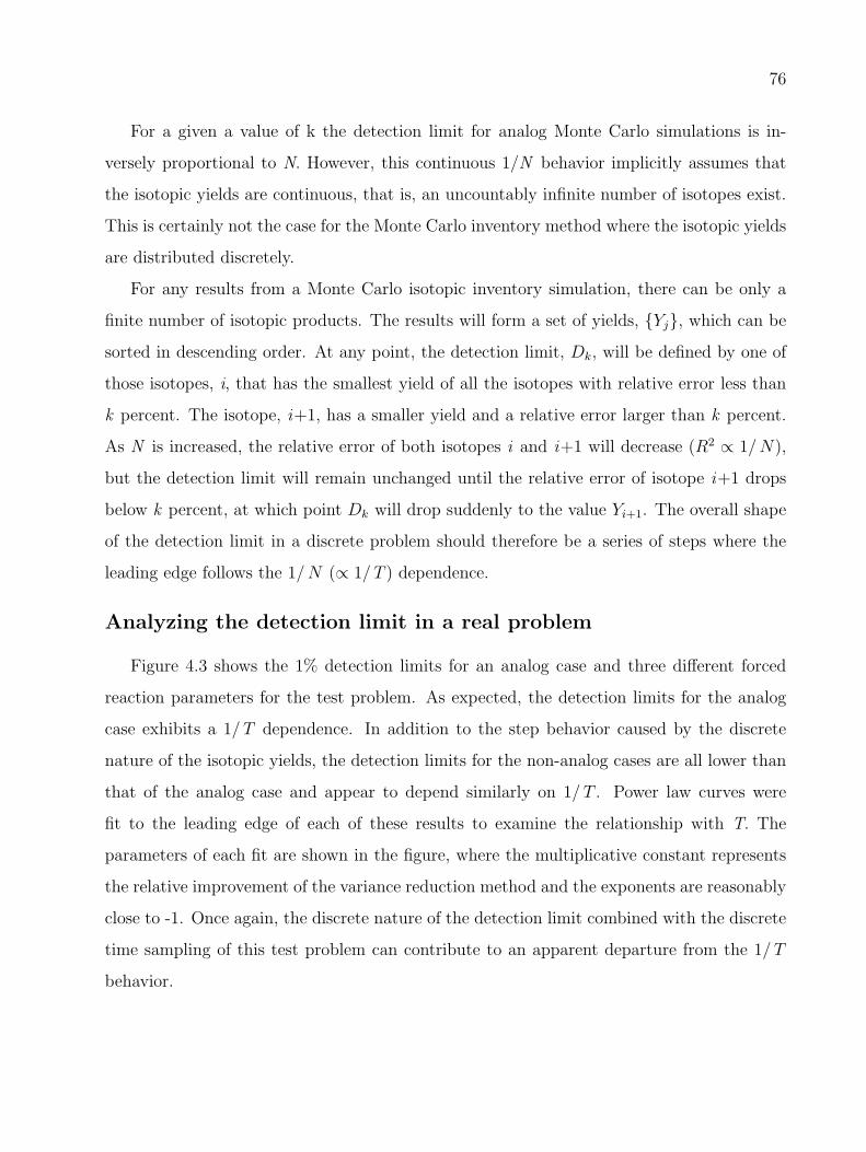
76

For a given a value of k the detection limit for analog Monte Carlo simulations is in-

versely proportional to N. However, this continuous 1/N behavior implicitly assumes that

the isotopic yields are continuous, that is, an uncountably infinite number of isotopes exist.

This is certainly not the case for the Monte Carlo inventory method where the isotopic yields

are distributed discretely.

For any results from a Monte Carlo isotopic inventory simulation, there can be only a

finite number of isotopic products. The results will form a set of yields, {Yj}, which can be

sorted in descending order. At any point, the detection limit, Dk, will be defined by one of

those isotopes, i, that has the smallest yield of all the isotopes with relative error less than

k percent. The isotope, i+1, has a smaller yield and a relative error larger than k percent.

As N is increased, the relative error of both isotopes i and i+1 will decrease (R2 ∝ 1/N),

but the detection limit will remain unchanged until the relative error of isotope i+1 drops

below k percent, at which point Dk will drop suddenly to the value Yi+1. The overall shape

of the detection limit in a discrete problem should therefore be a series of steps where the

leading edge follows the 1/N (∝ 1/ T ) dependence.

Analyzing the detection limit in a real problem

Figure 4.3 shows the 1% detection limits for an analog case and three different forced

reaction parameters for the test problem. As expected, the detection limits for the analog

case exhibits a 1/ T dependence. In addition to the step behavior caused by the discrete

nature of the isotopic yields, the detection limits for the non-analog cases are all lower than

that of the analog case and appear to depend similarly on 1/ T . Power law curves were

fit to the leading edge of each of these results to examine the relationship with T. The

parameters of each fit are shown in the figure, where the multiplicative constant represents

the relative improvement of the variance reduction method and the exponents are reasonably

close to -1. Once again, the discrete nature of the detection limit combined with the discrete

time sampling of this test problem can contribute to an apparent departure from the 1/ T

behavior.

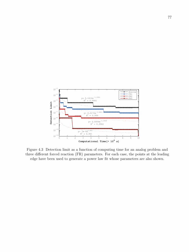
77

0 1 2 3 4 5 6 7 8 9 10

10-11

10 -10

10 -9

10 -8

10 -7

10 -6

10 -5

10 -4

10 -3

[× 104 s]

Detection Limit

AnalogFR1FR2FR5y= 0.1616x -1.0991

R2 = 0.9901

y= 0.0172x -1.0811

R2 = 0.999

y= 0.0004x -1.0059

R2 = 0.9962

y= 7e -6x -1.061

R2 = 0.961

Computational Time

Figure 4.3 Detection limit as a function of computing time for an analog problem andthree different forced reaction (FR) parameters. For each case, the points at the leading

edge have been used to generate a power law fit whose parameters are also shown.

78

0 1 2 3 4 5 6 7 8 9 10 11

100

102

104

106

108

Computational Time[× 104 s]

1 / DkT

Analog FR1 FR2 FR3 FR5 FR8

Figure 4.4 The detection limit based figure of merit is shown for the analog case and 5different forced reaction (FR) variance reduction parameters.

The detection limit, Dk, can be used to evaluate the overall performance of the modeling

scheme since a lower value Dk indicates a greater precision in the answer. In Figure 4.3,

orders of magnitude improvement are seen in the precision of the problem by invoking forced

reaction variance reduction. Because of the 1/ T dependence of the detection limit, the most

appropriate choice for a FOM is

FOM =1

Dk T(4.5)

This FOM for the various cases of the test problem are shown in Figure 4.4. As expected,

the overall shape of detection-limit-based FOM still exhibits the step behavior from 1/Dk.

However, the 1/ T factor helps to lessen a strong step-function behavior and causes the FOM

to oscillate about a constant value.

4.3.4 Error Corrected Detection Limit (1/DkR2T )

The fluctuations in the detection limit based FOM are due to the 1 /T factor while the

detection limit, Dk, is constant. Similarly, the relative error, Ri, of the isotope, i, that is

defining the detection limit is declining continuously with time while the detection limit is

constant at that isotope’s yield, Yi. It should therefore be possible to mitigate the oscillatory

79

0 1 2 3 4 5 6 7 8 9 10 11

106

108

1010

1012

[× 104 s]

1 / Dk R2 T

Analog FR1 FR2 FR3 FR5 FR8

Computational Time

Figure 4.5 Figure of merit using error corrected detection limit provides a measure of theoverall efficiency of the problem with a nearly constant value for a given modeling scheme.

behavior of the detection-limit-based FOM by using the relative error as a correction. In

particular, it can be shown that a figure of merit, 1/DkR2T , is constant for the analog case.

FOM =1

DkR2T(4.6)

In regions where Dk is constant, this FOM is constant since R2 behaves as 1/ T . Consider

how Dk and R2 vary across a jump in the detection limit:

D−k

D+k

≡ Yi

Yi+1

=Ni+1

Ni

=Ti+1

Ti

R2−

R2+

≡ R2i

k2= k2 Ti

Ti+1

1

k2=

Ti

Ti+1

,

∴ D−k R2

− = D+k R2

+ (4.7)

where D−k and D+

k are the detection limit on the left and right of the jump, respectively,

and R2− and R2

+ are the squares of the relative errors on the left and right of the jump,

respectively. Thus, for analog problems this FOM is constant across a jump in the detection

limit as well as during the periods where the detection limit does not change.

Figure 4.5 shows results for an FOM with this formulation. The results agree with the

analytic calculation that FOM is constant for analog case and nearly constant for the variance

80

reduction cases. Even though, this FOM is likely to experience some fluctuations due to the

discrete behavior of the detection limit, it can be used in a problem without a target isotope

to compare the overall efficiency of different schemes. Most importantly, it is effective at

providing an estimate of the necessary computing time for a given modeling technique to

achieve a certain overall precision, as indicated by the detection limit.

4.4 Summary

A number of statistical measures can be employed to assess the performance of different

Monte Carlo modeling schemes for a given isotopic inventory problem. From these, two

valuable figures of merit have been derived that meet the criteria described above: a figure

or merit should provide quantitative information about statistical performance, independent

of the number of simulated histories, providing guidance on the relationship between compu-

tational cost and performance. The FOM based on the relative error of a single tally result

(1/R2T ) is recommended for the problem with a known target isotope. In these situations,

the modeling scheme can be optimized for that single result and the necessary computing

time to achieve a target precision can be calculated. However, since many problems do not

have readily identified target isotopes, or may have multiple important isotopes, a FOM

based on the detection limit, corrected by the relative error, (1/DkR2T ) is useful for as-

sessing the overall efficiency of the problem. With this FOM, the modeling scheme can be

optimized against the detection limit and then the necessary computing time to achieve a

target detection limit can be calculated.

81

Chapter 5

Efficiency Assessment

This chapter uses the figures of merit defined in the previous chapter to evaluate the

possible computational efficiency improvements for a typical problem. A combination of

variance reduction techniques will be used, each with varying parameters, to determine a

best choice for different cases from a standard test problem. Study problem 1 is concerned

with a scenario in which a statistical quality of one specific isotopic product is of interest.

Study problem 2 is intended to study efficiency from using a reaction path splitting technique

as a means to improve the global efficiency of the Monte Carlo simulation. Both problems

illustrate how FOM responds to changing variance reduction parameters.

5.1 Problem Definitions

5.1.1 Standard test problem

A standard test problem is defined as the analog simulation in which isotopic inven-

tories following 10-year steady-state irradiation of 56Fe under a uniform neutron flux of

5×1012 n/cm2s are calculated. It is used in the study problems where each problem employs

a different set of variance reduction techniques. The FENDL-2/A activation library and

FENDL-2/D decay library are used.

5.1.2 Study problem 1

Following the irradiation in the standard test problem, several isotopic products are

selected such that their statistical errors are in distinctive ranges. Each chosen isotope is

82

assumed to be an isotope of interest in separate study cases. Each study case is composed of

many short test problems with different sets of variance reduction parameters. FOMs from

short test problems are used to determine a set of variance reduction parameters that yields

the most efficient scheme for producing that particular isotope. The forced reaction and

biased reaction branching techniques are used in all cases. The biased reaction branching

scheme is configured to increase the probability of the isotope of interest when it appears as

a product, but otherwise to invoke uniform reaction branching to ensure that each reaction

branch is followed with equal probability. The number of simulated particles in each short

test problem is 106.

5.1.3 Study problem 2

In this study problem, a forced reaction and reaction path splitting technique are applied

in the analog problem, aiming to obtain a deep and wide reaction tree. Six separate runs

are constructed from using different forced reaction parameters: 1, 2, 4, 6, 7 and 8. For each

run, an FOM, the error-corrected detection limit (1/DkR2T ), is calculated to quantitatively

evaluate the global efficiency. The number of simulated particles in each run is 105.

5.2 Simulation Results

5.2.1 Study problem 1

Based on an analog problem with 1010 simulated particles, four isotopes, 51Cr, 49Ti, 53Mn

and 60Ni, with statistical errors of 100%, 37.80%, 13.74% and 8.80%, respectively, were chosen

in the study. The reaction tree obtained from ALARA was used to make preliminary choices

for variance reduction parameter sets to be tested. In addition, the test sets were defined

based on an assumption that the overall statistical quality of a particular isotope depends

heavily on the qualities of the reaction branches that dominate the production of that isotope.

Thus, improving statistical qualities of those branches was likely to subsequently better the

statistical quality of the result.

83

CaseForced Biasing Relative Error FOM[s−1] FOM[s−1]

Parameter Score (%) 1/R2T 1/D1R2T

0 analog analog 100.00 4.98× 10−5 4.98× 105

1 3 5 8.95 2.4026 1.21× 1010

2 4 5 11.16 1.1158 1.21× 1010

3 5 5 32.42 0.1252 1.17× 1010

4 3 10 9.93 2.2060 1.50× 1010

5 4 10 5.28 5.9746 1.15× 1010

6 5 10 5.04 5.1763 1.18× 1010

7 3 100 15.79 0.9112 1.51× 1010

8 4 100 13.35 0.9355 1.63× 1010

9 5 100 11.21 1.0478 1.12× 1010

Table 5.1 The values of figure of merit (1/R2T ) were calculated from nine test runs andthe analog problem (1010 particles for case 0) when 51Cr was a target isotope. The valuesof one-percent error corrected detection limit (1/D1R

2T ) were included to compare thegeneral efficiencies of all test cases. One million simulated particles were used for each test

problem.

84

Target Isotope Dominant Reaction Chains

49Ti

56Fe → 52Cr → 49Ti

56Fe → 53Cr → 52Cr → 49Ti

56Fe → 53Cr → 50Ti → 49Ti

53Mn

56Fe → 55Fe → 55Mn → 54Mn → 53Mn

56Fe → 55Fe → 53Mn

56Fe → 55Fe → 54Fe → 53Mn

60Ni

56Fe →57Fe → 58Fe → 59Fe → 59Co

→ 60Co → 60Ni

56Fe → 57Fe → 58Fe → 59Fe → 59Co

→ 60mCo → 60Co → 60Ni

Table 5.2 Reaction channels leading to the most productions of 49Ti, 53Mn and 60Ni weredescribed and used for estimating the optimal values of variance reduction parameters.

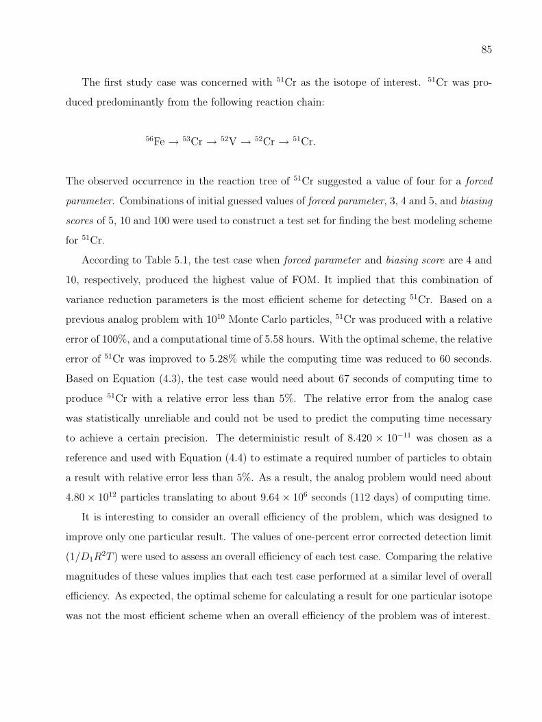
85

The first study case was concerned with 51Cr as the isotope of interest. 51Cr was pro-

duced predominantly from the following reaction chain:

56Fe → 53Cr → 52V → 52Cr → 51Cr.

The observed occurrence in the reaction tree of 51Cr suggested a value of four for a forced

parameter. Combinations of initial guessed values of forced parameter, 3, 4 and 5, and biasing

scores of 5, 10 and 100 were used to construct a test set for finding the best modeling scheme

for 51Cr.

According to Table 5.1, the test case when forced parameter and biasing score are 4 and

10, respectively, produced the highest value of FOM. It implied that this combination of

variance reduction parameters is the most efficient scheme for detecting 51Cr. Based on a

previous analog problem with 1010 Monte Carlo particles, 51Cr was produced with a relative

error of 100%, and a computational time of 5.58 hours. With the optimal scheme, the relative

error of 51Cr was improved to 5.28% while the computing time was reduced to 60 seconds.

Based on Equation (4.3), the test case would need about 67 seconds of computing time to

produce 51Cr with a relative error less than 5%. The relative error from the analog case

was statistically unreliable and could not be used to predict the computing time necessary

to achieve a certain precision. The deterministic result of 8.420 × 10−11 was chosen as a

reference and used with Equation (4.4) to estimate a required number of particles to obtain

a result with relative error less than 5%. As a result, the analog problem would need about

4.80× 1012 particles translating to about 9.64× 106 seconds (112 days) of computing time.

It is interesting to consider an overall efficiency of the problem, which was designed to

improve only one particular result. The values of one-percent error corrected detection limit

(1/D1R2T ) were used to assess an overall efficiency of each test case. Comparing the relative

magnitudes of these values implies that each test case performed at a similar level of overall

efficiency. As expected, the optimal scheme for calculating a result for one particular isotope

was not the most efficient scheme when an overall efficiency of the problem was of interest.

86

As stated, biased reaction branching was not applied at a reaction where 51Cr was not

present as a product. This has a negative impact on the performance compared to a case that

biases towards the pathways that eventually produce the target isotope. Further increase

in efficiency may be achieved with a more elaborately defined sets of variance reduction

parameters for every reaction.

Table 5.2 shows the reaction pathways with the most production of 49Ti, 53Mn and 60Ni.

It is important to point out that uniform reaction branching was not used in the study

case with 60Ni because both of the product channels in the chains resulting in 60Ni were

extremely active and thus probable. The use of uniform reaction branching would, in fact,

decrease frequency of 60Ni-terminated histories and consequently worsen the precision of

60Ni’s detection.

The most efficient sets of forced parameter and biasing score for calculating the inventories

of 49Ti, 53Mn and 60Ni were summarized in Table 5.3. With a simple application of variance

reduction techniques, as large as four orders of magnitude improvement in efficiency was

obtained in the study case of 49Ti. According to Table 5.4, the results of 49Ti and 60Ni showed

significant improvements in both statistical errors and computing time, with the statistical

errors errors under two percent and computing time of 54 and 136 seconds, respectively.

Although the statistical errors of 53Mn was only improved slightly, the computing time for

this studied isotope was greatly reduced from 5.58 hours to 54 seconds.

The simulation results confirmed the initial guess that the optimal values of forced pa-

rameter were in the proximity of the position of the target isotope in the dominant reaction

channels. For example, for 49Ti, the target isotope appeared 3th and 4th within the reaction

channels, and the optimal forced parameter for 49Ti is 3. On the other hand, the most effi-

cient choices of biasing score were determined on a trial-and-error basis. It was also worth

noting that the effect of biased reaction branching tended to be insignificant in a case when

a target isotope was the most active product. 60Ni was produced predominantly from a β−

decay of 60Co. This reaction channel was far more active than others of 60Co. A high value

of biasing score for this reaction channel would decrease the importance of each history due

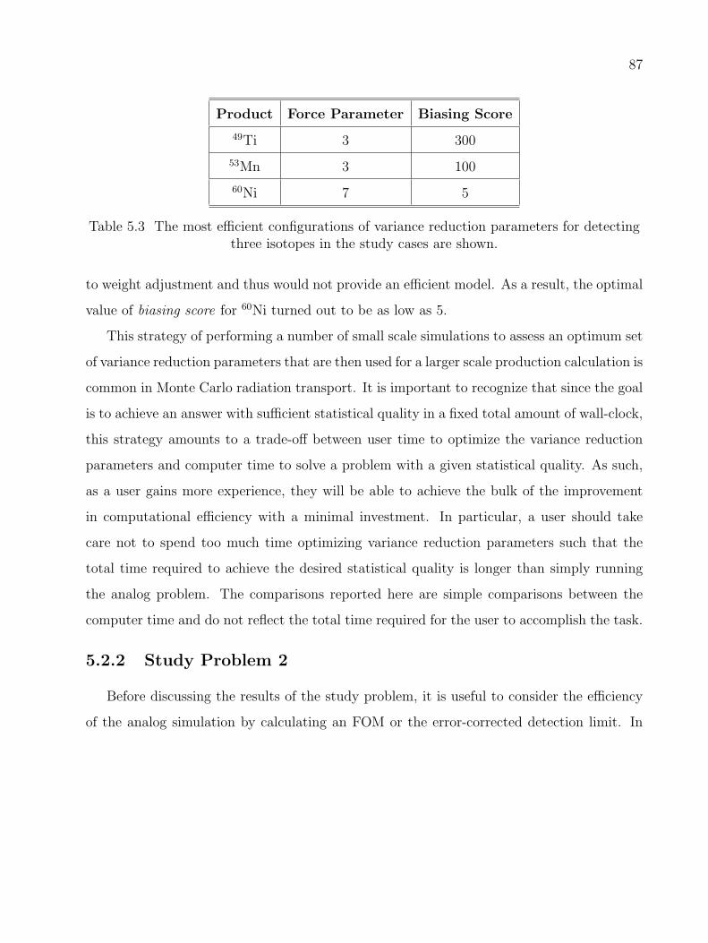
87

Product Force Parameter Biasing Score

49Ti 3 300

53Mn 3 100

60Ni 7 5

Table 5.3 The most efficient configurations of variance reduction parameters for detectingthree isotopes in the study cases are shown.

to weight adjustment and thus would not provide an efficient model. As a result, the optimal

value of biasing score for 60Ni turned out to be as low as 5.

This strategy of performing a number of small scale simulations to assess an optimum set

of variance reduction parameters that are then used for a larger scale production calculation is

common in Monte Carlo radiation transport. It is important to recognize that since the goal

is to achieve an answer with sufficient statistical quality in a fixed total amount of wall-clock,

this strategy amounts to a trade-off between user time to optimize the variance reduction

parameters and computer time to solve a problem with a given statistical quality. As such,

as a user gains more experience, they will be able to achieve the bulk of the improvement

in computational efficiency with a minimal investment. In particular, a user should take

care not to spend too much time optimizing variance reduction parameters such that the

total time required to achieve the desired statistical quality is longer than simply running

the analog problem. The comparisons reported here are simple comparisons between the

computer time and do not reflect the total time required for the user to accomplish the task.

5.2.2 Study Problem 2

Before discussing the results of the study problem, it is useful to consider the efficiency

of the analog simulation by calculating an FOM or the error-corrected detection limit. In

88

Product

Analog Problem Study Case

Relative Comp.F.O.M

Relative Comp.F.O.M

Error Time (s) Error Time (s)

51Cr 100% 20088 0.00005 5.28% 60 5.97

49Ti 30.15% 20088 0.00055 1.87% 54 52.76

53Mn 13.13% 20088 0.00290 11.08% 54 1.51

60Ni 8.64% 20088 0.00670 0.73% 136 139.37

Table 5.4 Comparisons of relative error, computing time and FOM between an analogproblem and study cases with optimal sets of variance reduction parameters are shown.

Improvements in all areas from the analog problem are observed in all cases.

CategoryStudy Case

F.P. 1 F.P. 2 F.P. 4 F.P. 6 F.P. 7 F.P. 8

Computing time (s) 192 274 3584 32902 97616 268823

Number of products 71 76 117 126 129 135

Dk, k = 10% 4.36e-13 1.92e-14 1.85e-21 1.93e-21 3.82e-28 4.19e-28

1/DkR2T , k = 10% 2.66e16 2.11e17 2.49e23 2.73e24 3.38e29 1.51e29

Dk, k = 5% 5.86e-9 4.09e-10 5.50e-17 1.93e-21 3.82e-28 4.19e-28

1/DkR2T , k = 5% 9.44e12 6.15e13 4.53e20 2.73e24 3.38e29 1.51e29

Table 5.5 Comparison of some characteristics of the results from the six study cases withdifferent force parameter.

89

this case, the FOM can be derived from Equation (4.4) and Equation (4.6) and given by

FOManalog =1

DkR2T

=N

1002k2

1002k2

T

=N

T(5.1)

where N is the number of histories and T is the total computing time. Since N is linearly

proportional to T , this quantity should always be constant. Based on the analog simulation

with 5 × 106 histories, the FOM is found to be 8.17e11. This FOM will later be used as

a basis to justify the efficiency gained for each study case. Note that for each study case

two values of FOMs are calculated: the error-corrected detection limit at 10% and 5%. A

magnitude comparison between these two FOMs provides a crude indication of the efficiency

limit for the current variance reduction techniques. That is, if the two values are exact, the

current simulation is unable to detect the next lowest product with a statistical error less

than 10%. Modifying parameters of the variance reduction techniques in use is not likely to

significantly decrease the detection limit, i.e. increase the efficiency.

Table 5.5 summarizes some characteristics of the results, which are important to the

efficiency assessment of the simulations. As expected, the numbers of products increase

with increasing force parameter. With higher force parameter, the simulation is able to

follow the particles deeper in a reaction tree and, at the same time, split the particles to

capture more possible reaction pathways. However, such an improvement is computationally

expensive as the computing time grows from 192 seconds to 74 hours when force parameter

is increased from 1 to 8, respectively. All FOMs from the study cases indicate that each

study case performs with a higher efficiency than the analog simulation. In addition, they

suggest that the study case with force parameter of 7 is the most efficient scheme. In fact, it

seems that a combination of forced reaction and reaction path splitting technique reaches its

efficiency limit when a force parameter is equal to 6 and both values of FOM are identical.

More evidently, the decreases in both FOMs after a force parameter of 7 indicate that

the simulation does not reduce the statistical errors as much as it increases the computing

90

time. Other variance reduction techniques are recommended for a further improvement in

efficiency. In this situation, a weight window technique is expected to be an appropriate

addition as it helps eliminate histories with insignificant weights.

5.3 Summary

A reaction tree from a deterministic calculation was an important input for defining an

initial set of variance reduction parameters to optimize the efficiency of production toward

one particular isotope. It was shown that an optimal value of forced parameters depended

on the position of that isotope in the reaction chain with the most relative production.

Another factor that influenced the efficiency was biasing scores, which were more difficult

to predict. The magnitude of biasing score of each reaction branch was likely to depend

on its relative contribution toward that isotope’s result. Improving the efficiency by all

means would likely require a priori knowledge of a reaction tree, which sometimes can be

computationally expensive.

A combination of forced reaction and reaction path splitting technique greatly broadens

and deepens a reaction tree, resulting in decreasing a detection limit and increasing a number

of isotopic products. The efficiency of this strategy is monitored by using FOM defined as

the error-corrected detection limit. Based on its defnition, this type of FOM can be used to

provide an estimate of the efficiency limit of the current variance reduction techniques.

91

Chapter 6

AVA: Adaptive Variance-reduction Adjustment

During the initial stage of MCise development, there are six different types of variance

reduction techniques. All of them have distinct advantages and require specific parameters to

operate. Optimizing these parameters by hand to create an efficient Monte Carlo simulation

for calculating a result of interest is a challenging task. For example, a simple simulation

might involve as many as thirty isotopes and each isotope is assumed to have ten possible

reaction products. The biased reaction technique, if used, needs three hundreds independent

parameters for each of the control volumes to make up a complete set of biasing scores. Such

a task is difficult to impossible to do within a reasonable amount of time. In fact, experts

in Monte Carlo transport, Booth and Hendricks, voice their opinion on selecting parameters

for variance reduction techniques and state, “The selection is more art than science, and

typically, the user makes a few short trial runs and uses the information these trials provide

to better guess the parameters; that is, the user learns to adjust parameters on the basis of

previous experience.”[14].

Fortunately, it is possible to develop an algorithm for the computer to recognize important

reaction pathways. The algorithm, which is described in more detail in the next section, is

called the Adaptive Variance-reduction Adjustment, or AVA for short. The algorithm is

an iterative process that adjusts variance reduction parameters for subsequent calculations

based on the information from a current short trial run. The algorithm is terminated when

a specific number of iterations or a desired efficiency are reached and a set of variance

92

Done?

AVAkernel

Input

FinalCalculation

Reaction tree

VR Parameters

Trial run

Isotopicresults

- problem definition- target isotope- tally bin

No

Yes

Figure 6.1 Data flowchart of AVA algorithm.

93

reduction parameters from the final iteration is used in an actual calculation with a much

higher number of simulated particles. The data flowchart of AVA is shown in Figure 6.1.

6.1 Algorithm

During the initial development stage of AVA, it was determined that an AVA scheme

should be intuitively simple and yet applicable to generic MCise simulations. More impor-

tantly, the scheme should be devised based on existing MCise capabilities. One possible

scheme was to exploit information from a reaction tree, which was automatically generated

during the simulation, to estimate importances of any isotopes to the production of a tar-

get result. These importances were used as primary inputs to define variance reduction

parameters.

AVA iteratively modifies complete sets of parameters for three different variance reduction

techniques to optimize the detection of a target isotope in a tally bin. The target isotope and

tally bin must be identified in advance for each specific problem. The techniques included

in AVA are forced reaction, biased reaction branching and biased source sampling. In each

AVA iteration, a short trial problem is simulated to obtain a reaction tree, generating tally

result in the bin of interest. Only valid reaction chains are extracted from the reaction tree.

The valid reaction chains are defined as linear reaction chains leading to the generation of

the target isotope in the specified tally bin. A sample schematic of valid reaction chains is

shown in Figure 6.2. Each valid reaction chain contains three types of nodes– a source node,

intermediate node and target node– and a relative contribution. The relative contribution

of any given valid reaction chain is defined as a fraction of the score of the target isotope

produced from that particular chain. Generally, a node carries an isotopic identity and

contains the hierarchical information about its parent and daughter nodes. A reaction chain

has only one source node and one target node, but may have multiple intermediate nodes

in the chain. Isotopic identities and physical locations of the nodes, along with relative

contributions from the reaction chains, are primarily used to initialize parameters for the

three variance reduction techniques as described below.

94

1

2

3

4

5

C1

C2

C3

C4

C5

Chain (i)SourceNode Intermediate Node Target Node

Relative Contribution (Ci)

Figure 6.2 A schematic illustration of reaction chains with relative contributions (Ci) tothe target isotope is shown. A gray, white and black circle represent a source, intermediate

and target node, respectively.

95

6.1.1 Forced Reaction

Since the sole purpose of a forced reaction technique is to force a simulated atom to

undergo a specific number of reactions, the numbers of reactions and relative contributions

from reaction chains are primarily inputs used to define a parameter for this technique.

A force reaction parameter is defined as the weight-averaged number of reactions among

the valid reaction chains. Its mathematical expression is given below:

Force Parameter =k∑

i=1

(ni + 1)Ci, (6.1)

ni = a number of intermediate nodes in the ith chain,

Ci = a relative contribution to the target result from the ith chain,

k = a total number of valid chains.

This initialization is designed to give considerations to all valid reaction chains, yet em-

phasize the ones with highest relative contributions. It implies that the simulation does not

force the simulated atoms to have many more reactions than the length of the reaction chain

that dominates the production of the target result. Note that the algorithm’s performance

matches the experience of previous chapters under these conditions.

6.1.2 Biased Reaction Branching

Typically, at any reaction point a reacting atom will be randomly assigned a new iso-

topic identity from a discrete probability density function (PDF) based on a list of possible

products. The PDF is calculated from the individual pathway cross-sections weighted by the

current neutron flux and/or decay rates. However, during an MCise simulation, this PDF

can be artificially modified by using a biased reaction branching technique. This technique

alters the PDF in favor of specified product isotopes and appropriately adjusts the weight

of a resultant product to ensure a fair simulation.

AVA uses information from the extracted reaction chains to define degrees of preference of

all product isotopes. The degrees of preference are subsequently used during the simulation

96

by a biased branching technique when it is modifying a discrete PDF for sampling a reaction

product. A probability of sampling each possible product at any reaction point is set to be

equal to its normalized degree of preference. For example, it is assumed that only isotopes,

a, b and c, have degrees of preference of Da, Db and Dc, respectively. A parent isotope, x, is

having a reaction and its possible daughter products are isotopes, a, b and f . In this case,

the sampling probabilities of a, b and c are given by Da

Da+Db, Db

Da+Dband 0 and correspond

to Bxa, Bxb and Bxf from the definition of Bij in Equation 3.8. Nonetheless, the analog

sampling is used if all of possible daughter isotopes has degree of preference equal to zero.

The degree of preference is designed based on an assumption that increasing simulated

populations of isotopes in the chains leading to the target isotope results in a more efficient

simulation for detecting the target isotope. Therefore, the degree of preference of a product

isotope is derived from the occurrences of the product isotope in the chains and the chains’

relative contributions to the target result. A degree of preference of an isotope j is defined

as a relative frequency of nodes representing an isotope j in a chain weighted-averaged by

the chain’s relative contribution. Mathematically, the degree of preference of any product

isotope j is given by:

Dj =k∑

i=1

δij

mi

Ci, (6.2)

Ci = a relative contribution from the ith valid chain,

k = a total number of valid chains,

δij = a number of nodes that represent the isotope j in the ith valid chain,

mi = a total number of nodes in the ith chain.

A fraction number of nodes is used, instead of a number of nodes representing a particular

isotope, to prevent AVA from assigning too high preferences for product isotopes in the long

valid chains. In addition, it preserves relative importances among the valid chains, based on

their relative contributions, Ci.

97

6.1.3 Biased Source Sampling

Currently, an isotopic identity of a source atom in an analog MCise simulation is randomly

sampled from a discrete PDF characterizing the isotopic compositions of the initial material.

The biased source sampling technique is implemented to help increasing the likelihood of

sampling the initial isotopes of interest. During an AVA process, this technique uses infor-

mation from AVA to adjust an underlying discrete PDF of the initial source composition,

aiming to improve statistics of the target result.

AVA provides degrees of preference of all source isotopes for the biased source sampling

technique, using a similar approach to the biased reaction branching technique. In this case,

only source nodes and relative contributions from the reaction chains are considered. A

degree of preference of a source isotope j is defined as the sum of relative contributions from

all valid reaction chains that have a source isotope as a source node. Mathematically, a

degree of preference of a source isotope j is expressed by the following:

Dj =k∑

i=1

βijCi, (6.3)

Ci = a relative contribution from the ith valid chain,

k = a total number of valid chains,

βij =

1, if the isotope j is a source isotope for the ith valid chain,

0, otherwise.

The degree of preference is designed such that a source isotope occurring more frequently

and heading the valid reaction chain with a higher relative contribution is given a higher

importance. This implementation ensures that reaction chains, which dominate the target

result, are more likely to be followed more often than those reaction chains with smaller

relative contributions.

98

6.2 Sample Problems

Two sample problems were designed to test the performance of AVA in two areas. The

first problem focused on the ability of AVA to adjust biasing scores for biased source sampling.

The inventory of 53Mn at shutdown following a 10-year steady-state of a mixture with a

uniform multi-group neutron flux of 5 × 1012n/cm2s was calculated from a problem using

AVA. The mixture was made up of equal atom fractions of chromium1, manganese2, iron3,

cobalt4 and nickel5. The test problem was defined to have ten iterations and each iteration

ran for 103 NPS. Prior to the AVA process, uniform reaction branching, uniform source

sampling and forced reaction with a force parameter of one were initially applied to generate

inputs necessary to define parameters for the first iteration. Biased reaction branching was

turned off during the AVA iterations. The final set of parameters from AVA would be applied

in the problem with 105 NPS. The result would then be compared with a deterministic

relative production of 4.505× 10−5 from ALARA.

The second problem had the same description as the first one except that the activated

mixture was replaced with 56Fe to simplify the source definition of the problem. This problem

focused on the ability of AVA to adjust biasing scores for biased reaction branching. A

deterministic relative production from ALARA for this case was 6.1× 10−9.

6.3 Results and Discussions

The value of NPS used in the preliminary run was set to be ten times higher than the

one used during AVA iterations. It initialized the set of parameters which would be updated

in subsequent AVA iterations. The larger amount of NPS is expected to provide good initial

estimates of the parameters, which in turn should give a final result with smaller statistical

error.

1Atom percent abundances: 50Cr - 4.35%, 52Cr - 83.79%, 53Cr - 9.50% and 54Cr - 2.36%2Atom percent abundance: 55Mn - 100%3Atom percent abundances: 56Fe - 91.75%, 54Fe - 5.85%, 57Fe - 2.12% and 58Fe - 0.28%4Atom percent abundance: 59Co - 100%5Atom percent abundances: 58Ni - 68.08%, 60Ni - 26.22%, 61Ni - 1.14%, 62Ni - 3.63% and 64Ni - 0.93%

99

0 2 4 6 8 10 1210-20

10 -15

10 -10

10 -5

100

Iteration

Source Sampling Probability

55Mn54Fe56Fe58Ni60Ni

Figure 6.3 Probabilities of source sampling from the first sample problem were shown as afunction of iterations. There were five source isotopes present after the preliminary run.

Each iteration was run for 104 NPS.

A preliminary run from the first test problem produced twenty five reaction chains lead-

ing to the production of 53Mn. Out of fifteen possible source isotopes, 54Fe, 55Mn, 58Ni,

56Fe and 60Ni, in an increasing order of relative contributions, were found at the top of

those reaction chains. The probabilities for source sampling were initialized and iteratively

increased according to Equation (6.3). The evolutions of those probabilities are illustrated

in Figure 6.3.

Probabilities for sampling 54Fe heavily dominated other probabilities at all iterations.

They contributed to the fact that 53Mn occurred predominantly from two reactions: 54Fe(n,np)−→

53Mn and 54Fe(n,d)−→ 53Mn. Increasing frequencies of source isotopes leading to 53Mn was the

only means to statistically improve its result since biased reaction branching was unavail-

able. The other source isotope that was significant to the production of 53Mn was 55Mn by

a reaction, 55Mn(n,2n)−→ 54Mn

(n,2n)−→ 53Mn. At the end of the AVA process, the probabilities for

source sampling 54Fe and 55Mn were approximately 96.30% and 3.70% while the probabilities

for other sources were extremely small that could be negligible. The final value of the force

100

0 2 4 6 8 10

0

0.05

0.1

0.15

0.2

0.25

0.3

0.35

Iteration

Reaction Branching Probability 53Mn

54Mn55Mn53Fe54Fe55Fe56Fe

Figure 6.4 Probabilities of reaction branching from the second sample problem were shown.

101

parameter was 1.00675 which agreed with a physical observation that a majority of 53Mn

was from a two-node reaction chain starting with 54Fe.

The inventory of 53Mn from the final calculation was 4.512× 10−5 with a statistical error

of 1.09%. The result was in great agreement with the deterministic result as the relative

difference was 0.16%. The simulation required a total computing time of 5.97 seconds,

including the AVA process, to achieve these levels of accuracy and precision. To evaluate the

efficiency of AVA, an analog problem with 107 NPS was run and timed with a computing

time of 35.71 seconds. The analog problem would require at least 1.87× 108 NPS if it were

to reproduce the result of 53Mn with the same accuracy and precision. This amount of NPS

translated into a computing time of about 668 seconds. The difference of those computing

times showed that AVA performed with a reasonable efficiency.

The next test problem involved adjusting biasing scores for biased reaction branching.

Once again, a preliminary run preceding the AVA was required. Initially, five valid reaction

chains containing nineteen nodes were obtained. Each node was considered to initialize a

probability for sampling a reaction product in favor of its corresponding isotope, according

to Equation (6.2). The initial force parameter was initialized to be 2.514. After all, seven

different isotopes were given initial probabilities which would be thr basis for subsequent

AVA iterations. Those seven isotopes included a source isotope, 56Fe, a target isotope,

53Mn, and five intermediate isotopes, 54Mn, 55Mn, 53Fe, 54Fe, and 55Fe. The first AVA

iteration produced nineteen valid reaction chains; however, there were only two different

parent isotopes, 55Fe and 54Mn, in those chains before the target. Almost all occurrences

of 55Fe came from the reaction chain, 56Fe(n,2n)−→ 55Fe

(n,t)−→ 53Mn. On the other hand, 54Mn

appeared in many reaction chains due to an active loop reaction, 54Mn(n,2n)−−−−⇀↽−−−−(n,γ)

53Mn. The

sizes of those reaction chains ranged from three to seven nodes. The probability progressions

of all seven isotopes at all iterations were shown in Figure 6.4.

Expectedly, biasing probabilities for 56Fe and 53Mn were higher than others since they

appeared in every valid reaction chain as a source and target node, respectively. Overall,

marginal changes of probabilities were observed after the first iteration and the probabilities

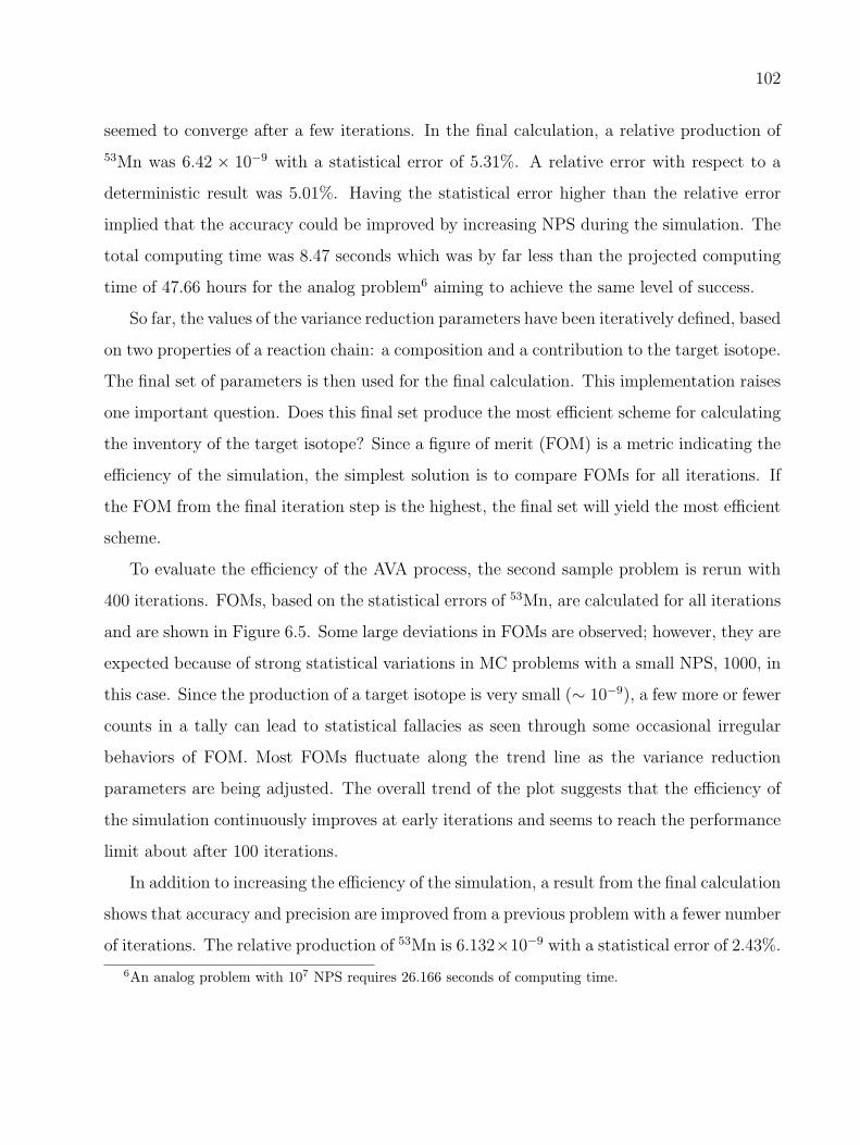
102

seemed to converge after a few iterations. In the final calculation, a relative production of

53Mn was 6.42 × 10−9 with a statistical error of 5.31%. A relative error with respect to a

deterministic result was 5.01%. Having the statistical error higher than the relative error

implied that the accuracy could be improved by increasing NPS during the simulation. The

total computing time was 8.47 seconds which was by far less than the projected computing

time of 47.66 hours for the analog problem6 aiming to achieve the same level of success.

So far, the values of the variance reduction parameters have been iteratively defined, based

on two properties of a reaction chain: a composition and a contribution to the target isotope.

The final set of parameters is then used for the final calculation. This implementation raises

one important question. Does this final set produce the most efficient scheme for calculating

the inventory of the target isotope? Since a figure of merit (FOM) is a metric indicating the

efficiency of the simulation, the simplest solution is to compare FOMs for all iterations. If

the FOM from the final iteration step is the highest, the final set will yield the most efficient

scheme.

To evaluate the efficiency of the AVA process, the second sample problem is rerun with

400 iterations. FOMs, based on the statistical errors of 53Mn, are calculated for all iterations

and are shown in Figure 6.5. Some large deviations in FOMs are observed; however, they are

expected because of strong statistical variations in MC problems with a small NPS, 1000, in

this case. Since the production of a target isotope is very small (∼ 10−9), a few more or fewer

counts in a tally can lead to statistical fallacies as seen through some occasional irregular

behaviors of FOM. Most FOMs fluctuate along the trend line as the variance reduction

parameters are being adjusted. The overall trend of the plot suggests that the efficiency of

the simulation continuously improves at early iterations and seems to reach the performance

limit about after 100 iterations.

In addition to increasing the efficiency of the simulation, a result from the final calculation

shows that accuracy and precision are improved from a previous problem with a fewer number

of iterations. The relative production of 53Mn is 6.132×10−9 with a statistical error of 2.43%.

6An analog problem with 107 NPS requires 26.166 seconds of computing time.

103

0 100 200 300 400

1000

2000

3000

4000

Iteration

Figure of Merit

Figure 6.5 Figures of merit from the second sample problem with 400 iterations are shown.Note that FOMs are based on the statistical errors of 53Mn and a dash red line indicates

the overall trend of FOMs.

104

When compared to the deterministic result, a relative error is found to be 0.525%. The total

computing time is 29.18 seconds.

6.4 Summary

To employ variance reduction techniques to the highest capabilities, their parameters

must be properly defined. Traditionally, the parameters have been computed manually.

First, the initial set of parameters is derived from intuition and experience. A short problem

is run and its result is considered to determine whether or not it is satisfactory. If not, those

parameters are re-adjusted. AVA is developed to eliminate the guesswork in developing

the initial set of parameters and a series of trials for manually adjusting those parameters.

Based on two sample problems, AVA is successfully implemented to define an efficient set

of parameters for forced reaction, biased reaction branching and biased source sampling

techniques. Precision and accuracy of AVA problems are greatly improved from an analog

problem as evident from dramatic decreases in both computing time and relative error.

105

Chapter 7

Applications

In this chapter, isotopic inventories of three systems with flowing materials are examined

to demonstrate capabilities of MCise in modeling the activation process without having to

deploy approximation strategies on an irradiation schedule. The first system is a hypothetical

problem taken from Introduction to Nuclear Engineering 2nd Edition by John R. Lamarsh

(Problem 10.35)[23]. In this problem, an activity at equilibrium is determined analytically,

and is compared to a numerical result from MCise. This problem serves as a good benchmark

for MCise because an analytical solution can be derived. The second system involves the

study of transmutation and burnup of liquid fuel in In-Zinerator [24]. This system poses a

unique challenge in that the model must incorporate the on-line fission product separation

and time-dependent continuous feed of fresh fuel hoping to keep a thermal power constant.

Lastly, the activation assessment of a LiPb liquid breeder in the ARIES compact stellarator

power plant or ARIES-CS [25] is investigated. A challenge in modeling this system is due to

the fact that the breeder passes through two different radial blankets and hence experiences

two different spectrums. Two outflows then mix in the external vessel where tritium is

extracted and re-enter the blankets.

7.1 Coolant Activation

The problem description below is excerpted from Introduction to Nuclear Engineering

2nd Edition by John R. Lamarsh (Problem 10.35):

106

Core tc

Reflectortr

to

fc

fr

α

Figure 7.1 The coolant circuit is composed of core, reflector and outer circuit.

In many water cooled reactors the water acts as moderator and reflector as well as

coolant. The coolant circuit is then as shown in [Figure 7.1], where the fraction

fc of the coolant entering the reactor passes through the core, the remaining

fraction fr going to the reflector. The average activation rates per unit volume in

the core and reflector are (Σactφav)c and (Σactφav)r, respectively, and the water

spends the times tc, tr and to in the core, reflector and outer circuit. Show that

the specific activity leaving the reactor is given by

α =fc(Σactφav)c(1− e−λtc) + fr(Σactφav)r(1− e−λtr)

1− fce−λ(tc+to) − fre−λ(tr+to). (7.1)

7.1.1 Problem Modifications

Several modifications are made to the problem so that the comparison between analytical

and MCise results are well presented. These modifications are described as follows.

Neutron Flux

The neutron fluxes in the core and the reflector in this study are obtained from the real

values in the University of Wisconsin’s Nuclear Reactor. 1 The flux is normalized to simulate

an energy production of 1000 MWth, as shown in Figure 7.2. Although these values are not

1Benjamin Schmitt, a UWNR operator, provides the sample neutron fluxes.

107

perfect representatives of the operational fluxes in the actual power plants, they are readily

available and are sufficient for our purposes.

Coolant

In general, there are a few important reactions by which coolants are activated [23]:

16O(n,p)16N, 17O(n,p)17N, 18O(n,γ)19O, 23Na(n,γ)24Na and 40Ar(n,γ)41Ar. The first three

reactions are the primary sources of radioactivity in the water cooled reactor while the

last two reactions are significant contributors in the reactors with sodium and air coolant,

respectively. In the context of this exercise, a sodium activation has a distinct advantage over

oxygen activation because its activation can occur with neutrons at all energies. Therefore,

sodium coolant is assumed to be used and a reaction, 23Na(n,γ)24Na, is considered.

Output Response

The amount of 24Na relative to an initial amount of 23Na is the current output response

from MCise tally. The final solution in (7.1) must be manipulated to give the answer com-

parable to the output from MCise. Terms, (Σactφav)c and (Σactφav)r, must be replaced with

the effective reaction rate coefficients for a reaction, 23Na(n,γ)−→ 24Na, in the core and reflector,

respectively. They can be calculated by collapsing the (n, γ) cross section with the neutron

fluxes for the core and reflector. With simple manipulations on Equation (7.1), the relative

amount of 24Na is given by

NNa−24

NNa−23

=fc

(σγφav)c

λ(1− e−λtc) + fr

(σγφav)r

λ(1− e−λtr)

1− fce−λ(tc+to) − fre−λ(tr+to). (7.2)

7.1.2 MCise Simulation

To construct the model in MCise, the initial values for the variables are assigned in Ta-

ble 7.1. Note that a parametric study can be performed by varying each variable in question

individually while keeping other variables fixed. Three control volumes are defined to rep-

resent components through which simulated atoms must progress. The core and reflector

108

10-12

10 -10

10 -8

10- 6

10- 4

10-2

100

102

1012

1013

1014

1015

Energy (MeV)

Magnitude (n/cm2s)

ReflectorCore

Figure 7.2 Sample neutron fluxes are taken from UWNR and normalized to an operatingcondition of 1000 MW.

Variable Value

tc 2600 s

tr 3600 s

to 1000 s

fc 50%

fr 50%

Table 7.1 Residence times in the core, reactor and outer circuit, and relative volumetricflow rates in the core and reactor are assumed.

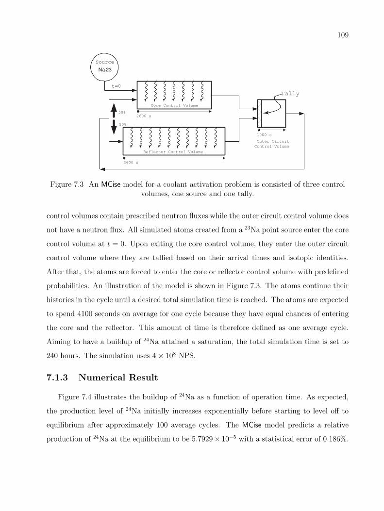
109

Tally

Source

Na-23

Core Control Volume

Reflector Control Volume

Outer Circuit

Control Volume

1000 s

2600 s

3600 s

50%

50%

t=0

Figure 7.3 An MCise model for a coolant activation problem is consisted of three controlvolumes, one source and one tally.

control volumes contain prescribed neutron fluxes while the outer circuit control volume does

not have a neutron flux. All simulated atoms created from a 23Na point source enter the core

control volume at t = 0. Upon exiting the core control volume, they enter the outer circuit

control volume where they are tallied based on their arrival times and isotopic identities.

After that, the atoms are forced to enter the core or reflector control volume with predefined

probabilities. An illustration of the model is shown in Figure 7.3. The atoms continue their

histories in the cycle until a desired total simulation time is reached. The atoms are expected

to spend 4100 seconds on average for one cycle because they have equal chances of entering

the core and the reflector. This amount of time is therefore defined as one average cycle.

Aiming to have a buildup of 24Na attained a saturation, the total simulation time is set to

240 hours. The simulation uses 4× 108 NPS.

7.1.3 Numerical Result

Figure 7.4 illustrates the buildup of 24Na as a function of operation time. As expected,

the production level of 24Na initially increases exponentially before starting to level off to

equilibrium after approximately 100 average cycles. The MCise model predicts a relative

production of 24Na at the equilibrium to be 5.7929× 10−5 with a statistical error of 0.186%.

110

0 40 80 120 160 200 2400

2

4

6

x 10-5

Operation time (hr)

Atomic concentration of 24Na

1 average cycle = 4100 s

50 average cycles

100 average cycles

200 average cycles

Analytical Result at Equilibrium5.8152

MCise Result

Figure 7.4 A atomic concentration of 24Na from MCise is plotted as a function of operationtime. A dash-dot line indicates a relative production at equilibrium from a deterministic

calculation.

111

This numerical result is in remarkable agreement with the result of 5.812× 10−5 calculated

using the deterministic model. However, a high-frequency fluctuation at the equilibrium

observed in the MCise result with this small statistical error is not typical. After a careful

review of the problem description, the reasoning behind this unusual characteristic can be

explained as follows.

As the coolant leaves the outer circuit control volume, it faces a decision whether to

enter the reflector or the core control volume. In MCise model, the probabilities of entering

either control volumes is assumed to be the same. Each particle history can be viewed

as a unique physical realization of a stochastic irradiation history. The statistical nature

of the problem requires large numbers of physical realizations to see convergence, adding

significant complication to the calculation. In this particular case, a number of required

physical realizations can be calculated and given by 2k, where k is a number of cycles. As

the system reaches equilibrium, the number of possible physical realizations grows to about

2100, which is in the order of 1030. This situation in the inventory analysis is analogous to

that of particle transport in stochastic mixtures[26].

To attain the ensemble average of the solution is a simple but extremely computationally

expensive procedure– a Monte Carlo simulation and tally of the quantities of interest is

recorded for each particular physical realization before averaging. Given infinite computing

resources, this procedure yields the exact solution. Nevertheless, it is clearly impractical for

routine use. Therefore, many efficient algorithms have been developed to produce reasonable

approximations to the exact solution. An algorithm proposed by Zimmerman[27] and its

later extensions by Donovan and Danon[28] are based on the use of a chord-length sampling

technique to avoid the need to create a set of physical realizations in order to obtain the

solution. This problem is a potential research direction for inventory analysis which requires

further extensive investigation and is beyond the scope of this thesis.

112

D-T Target D-T Target500 cm

200 cm

Coolant Blanket

Reflector

Fuel Tubes

Hasteloy-N Wall

Figure 7.5 Axial and radial cross section of the MCNP model of the In-Zinerator.

7.2 In-Zinerator

The Z-pinch transmuter uses a D-T fusion target, which produces a point source of 14.1-

MeV neutrons, to drive sub-critical cylindrical channels containing actinides in a fluid form.

The 200-MJ fusion target is ignited every ten seconds to provide a 20-MW fusion source for

the blanket. The In-Zinerator, with its MCNP model shown in Figure 7.5, is designed to

keep the channels sub-critical and to maintain a desired power level of 3000 MWth. The

fusion target is located in the center of the chamber and is 2 meters from the first wall. The

first wall is a 5-cm thick cylindrical sheet of Hasteloy-N. The coolant blanket is 57-cm thick.

The actinides are contained in a fluid fuel form within 1150 tubes in the blanket. Each tube

is made of Hasteloy-N and has an inner and outer radius of 2.2 cm and 2.4 cm, respectively.

Surrounding the coolant blanket are a 50-cm and 5-cm thick layer of lead and Hasteloy-N,

respectively. The former serves as a reflector to increase neutron multiplications.

The liquid fuel is an eutectic at 675 ◦C formed by LiF and AnF3 (actinides fluoride) with

a molar ratio of 2 to 1. Actinides in the problem are made of transuranic isotopes(TRU) from

spent LWR fuel. One advantage of liquid fuel is that, a portion of fluid can be taken out of

the reactor and processed to remove fission products. The processed fuel is then replenished

113

Fresh TRUFeed FP

ExtractionReactor Core

tr

FPSink

Initial Core Loading

Figure 7.6 Schematic of In-Zinerator MCise model, showing sources in red and sinks inblue.

with some fresh TRU necessary to maintain constant inventories and returns to the reactor.

While most, if not all, traditional tools are not suitable for performing activation and burnup

calculation on this type of fuel cycle, MCise is implemented with capabilities to handle online

material addition into and extraction out of the system.

The goal of this study problem is to use MCise to calculate detailed isotopic distributions

at all operation times.

7.2.1 MCise Simulation

A schematic of the MCise model of the In-Zinerator is illustrated in Figure 7.6. The

two control volumes in this schematic are the reactor core and fission product extraction

environments. The reactor core is characterized by the average neutron flux that the eutectic

fuel experiences while the second control volume has a neutron flux of zero. For the purpose

of this analysis, a residence time of 100 days in the reactor was chosen corresponding to the

processing of 1% of the total inventory per day in the fission product extraction step. The

residence time of the FP extraction represents a processing period of the fuel and was chosen

to be zero during the initial stages of this study.

All of the flow leaving the reactor core goes to the FP extraction process, but the flow

leaving the FP extraction process is divided into two streams based on the atomic species.

All fission products flow to the sink and all actinides (and Li and F) are returned to the

reactor core. This model was chosen to represent an ideal separations process and the flow

distribution of each species can be adjusted to represent the real separations efficiencies.

114

There are two atom sources in the In-Zinerator model. Isotopic distributions of both

sources are summarized in Table 7.2.

The first one is the source representing the isotopic mix of the initial core loading and

is assigned to the reactor core control volume. Mathematically, its time-dependent source

strength is defined as

r1(tsim) = R1δ(tsim), (7.3)

where R1 is the total number of atoms at the initial core loading. Since the atoms sampled

from this source would start their history uniformly inside the reactor core, a PDF describing

their remaining residence time is given by:

p1(trem) = 1/tr. (7.4)

The other source accounts for the addition of fresh fuel (TRU) to replace the consumed

fuel. For this model, it was assumed that actinides could only be added as rapidly as

fission products were being removed, to maintain a constant inventory in the reactor. More

precisely, since each actinide fission results in two fission products, the rate of addition of

actinides should be half the rate of removal of fission products. The fission product removal

rate is determined by the inventory of fission products in the system. Under the assumption

of a constant power level in the reactor, this can be calculated analytically:

F = κP − εC

IF, (7.5)

F (0) = 0, (7.6)

115

IsotopeInitial Core Loading Feed Stream

(atomic fraction) (atomic fraction)

Li-6 1.2501e-2 -

Li-7 2.3753e-1 -

F-19 6.2507e-1 -

Np-236 9.0012e-9 7.3147e-8

Np-237 9.0761e-3 7.3435e-2

Np-238 - 3.1085e-11

Np-239 - 1.7966e-8

Pu-236 - 1.4384e-12

Pu-238 3.3129e-3 2.6630e-2

Pu-239 5.6632e-2 4.5452e-1

Pu-240 3.2879e-2 2.6288e-1

Pu-241 1.1576e-3 9.2095e-3

Pu-242 7.2382e-3 5.7352e-2

Pu-243 1.4127e-6 1.3491e-16

Pu-244 - 1.1055e-5

Am-241 1.1576e-2 9.2075e-2

Am-242 2.0627e-5 1.9542e-9

Am-242m - 1.6305e-4

Am-243 2.6003e-3 2.0530e-2

Am-244 - 1.5457E-20

Cm-242 4.9754e-8 3.9434e-7

Cm-243 3.5004e-6 2.7573e-5

Cm-244 2.6878e-4 2.1100e-3

Cm-245 1.1051e-4 8.6423e-4

Cm-246 2.4878e-5 1.9336e-4

Cm-247 4.8005e-7 3.7225e-6

Cm-248 5.5381e-8 4.2804e-7

Bk-249 1.2501e-10 -

Cf-249 1.2501e-10 -

Cf-250 1.2501e-10 -

Table 7.2 Isotopic compositions of sources used in the MCise simulation are shown.

116

where

F = a total inventory of fission products [atoms]

P = a desired power level [energy/time]

κ = a number of fission products produced for an average fission energy released

≈ 2

180MeVatoms/energy

ε = an efficiency of a fission product separation process [dimensionless]

C = a processing capacity rate [atoms/time]

I = a total initial inventory [atoms],

therefore,

F (t) =κPI

εC

(1− e−εCt/I

). (7.7)

The feed rate of fresh TRU needed is also equivalent to the time-dependent source

strength of the second source in the MCise simulation and given by:

r2(tsim) =1

2

εC

IF (tsim) =

κP

2

(1− e−

εCtsimI

), 0 < tsim < Tsim. (7.8)

Since the feed stream always enters at the beginning of the reactor control volume, a

PDF describing the remaining residence time of the feed is defined with a delta function,

p2(trem) = δ(trem − tr). (7.9)

The CINDER90 nuclear data library is used in this study. It uses a 63 group energy

structure and includes both transmutation reactions and fission reactions with fission product

yields. The fission product yields are not explicitly dependent on the neutron flux spectrum,

but are defined for a number of representative spectrum types: thermal, fast and high-

energy. For some isotopes, spontaneous fission product yields are also given. CINDER

does not provide fission yields for all possible fission reactions. In such cases, when a fission

reaction occurs, the product isotopes will be assigned a placeholder isotopic identity, unknown

fission product. This isotope is stable and neutronically transparent and will accumulate. An

accumulation of this isotope could result in underestimating decay heat and specific activity

of the system.

117

Parameter Value Description

P 3.7233× 103 MWth

A F6 tally in MCNP is used to detect energy

absorption in the reactor structure. The fusion

source strength is taken to be 7.1× 1018s−1.

I 2.8293× 1029 A total number of atoms from the initial core loading

ε 100% Assumed

C I/100 day−1 Assumed

tr 100 days I/C

Table 7.3 Values for six parameters necessary for the MCise simulation are assumed andshown.

7.2.2 Analysis Methodology

As in any fissile system, a calculation of the long term isotopics requires a tight coupling

between the neutron transport calculation and the changing isotopics. In this system, jus-

tified in part by the constant replenishment of TRU fuel, the system was modeled with a

constant neutron flux, both magnitude and energy spectrum, and assumed to have a constant

power level. Even though the assumptions are not realistic, they provide a good starting

point for the analysis.

In addition to these assumptions, several key parameters must be assumed to initiate an

MCise simulation. Those parameters are summarized in Table 7.3. The neutron flux at the

initial core loading can be obtained from MCNP and is shown in Figure 7.7 using the same

63 energy groups defined by the CINDER data library.

Based on these assumptions and parameters, an MCise simulation is performed with a

constant neutron flux in the reactor core for 20,000 days of operation, with isotopic inventory

results recorded every 20 days.

118

10-8

10 -6

10 -4

10 -2

100

102105

107

109

1011

1013

1015

Energy (MeV)

Magnitude (n/cm2-s)

Figure 7.7 The initial flux is obtained from MCNP. The number of energy groups andenergy structures are in correspondence to a CINDER data format.

119

7.2.3 Results and Discussion

Results for the 11 isotopes with the highest concentrations and fission products are shown

in Figure 7.8. Fission products build up very rapidly at the beginning of the system’s life.

Many actinides approach equilibrium levels after about 10 years of operation. Other actinides

gradually reach the equilibrium at times closer to 30 years.

The tritium breeding ratio (TBR), energy multiplication and keff are calculated as a

function of time and are shown in Figures 7.9 to 7.11, respectively. Energy multiplication is

calculated by dividing the total thermal power, measured in MeV per source neutron (total

neutron and photon heating in entire problem geometry) by 12.8 MeV per source neutron

(the average neutron energy as it leaves the target region). Error bars in the figures represent

1σ statistical errors. These are calculated using MCNP with material compositions based

on the results of MCise.

Original results based on a replenishment of only TRU do not take into account the

substantial depletion of 6Li during the operation. This depletion is partly responsible for

a decrease in tritium breeding ratio and increase in energy multiplication. Results are also

shown with a constant 6Li inventory, based on the same MCise isotopic inventory results

but with the 6Li inventory maintained in the MCNP input file. As expected, the tritium

breeding ratio increases and equilibrium is reached within about 1 year based on the energy

multiplication and multiplication factor.

The rapid drop in energy multiplication at early times affects the fission product accumu-

lation. At early times, the fission product inventory increases towards an equilibrium value

that is a function of the power level. Since the power level drops on the same time scale that

the fission product inventory is accumulating, the fission product inventory reaches a level

that is higher than the long term equilibrium level and must drop to reach that level.

These results demonstrate that a reactivity control mechanism will be necessary to ensure

a constant energy multiplication over the life of the system. If such a mechanism were to

preserve the neutron energy spectrum and magnitude, then the modeling assumptions made

here would continue to be valid. However, preliminary results show that this may not

120

0 10 20 30 40 50 6010

24

1025

1026

1027

1028

1029

Operation Time (years)

Inventory (atoms)

Pu−238

Pu−239

Pu−240

Pu−241

Pu−242

Np−237

Am−241

Am−242m

Am−243

Cm−242

Cm−244

FP

Figure 7.8 Inventories of eleven isotopes with highest concentrations and fission productsas a function of operation times are shown.

121

0 400 800 1200 1600 2000

0.6

0.9

1.2

1.5

1.8

Operation Time (days)

TBR

TRU Feed TRU and Li−6 Feed

Figure 7.9 Tritium breeding ratio (TBR) for whole system, with and withoutreplenishment of 6Li.

0 200 400 600 800 1000 1200 1400 1600 1800 2000100

150

200

250

300

350

Operation Time (days)

Energy Multiplication

TRU Feed TRU and Li−6 Feed

Figure 7.10 Energy multiplication for whole system with and without replenishment of 6Li.

122

0 400 800 1200 1600 2000

0.960

0.965

0.970

0.975

0.980

0.985

0.990

Operation Time (days)

keff

TRU Feed TRU and Li−6 Feed

Figure 7.11 Total system multiplication factor with and without replenishment of 6Li.

123

be the case, requiring a tighter coupling between the neutronics, isotopics, and reactivity

configuration of the system.

An iterative calculation between MCNP and MCise must be employed to accurately

determine burnup and activation of the materials. The following iterative scheme is proposed

for the future work.

1. At time, ti, use MCNP to iteratively find the reactivity control state, Si, that achieves

a desired energy multiplication for the current isotopic inventory state, Ii,

2. Use the neutron flux from step 1 with MCise to determine isotopic distributions for the

next time step, Ii+1.

7.3 ARIES-CS

This problem is developed to assess the activation level of LiPb liquid breeder in ARIES-

CS. In this system, the breeder consistently flows into and out of two radial breeding zones

for on-line tritium removal. As the breeder returns to the breeding zones, it may not enter

the same zone it previously exits. In addition, the ARIES-CS neutronics is radially de-

pendent; therefore, the breeding zones have different spectra. This flowing nature makes

it impossible for a deterministic activation code to design an exact pulsing schedule for a

realistic irradiation history. On the other hand, MCise is able to follow histories of individual

atoms as they go through a network of different irradiation volumes. Therefore, MCise can

realistically model this type of system by taking advantages of its underlying methodology,

which does not require a definition of an irradiation schedule.

7.3.1 MCise Simulation

This study problem is based on an ongoing development of ARIES-CS, whose radial

builds and compositions are fully described in [29]. Only aspects of ARIES-CS relevant to

the MCise simulation are discussed here.

124

Element Weight Fraction(%)

Pb 99.29

Li 0.70

Zn 1e-3

Fe 1e-3

Bi 4.3e-3

Cd 5e-4

Ag 5e-4

Sn 5e-4

Ni 2e-4

Table 7.4 Isotopic compositions of the LiPb liquid breeder. Li is 90-percent enrichmentwith 6Li. The theoretical density is 8.80 g/cm3.

125

In the most recent ARIES-CS design, the LiPb liquid breeder flows through in-blanket

and ex-vessel where it spends 1 and 1.5 minutes, respectively. The in-blanket contains

two tritium-breeding zones. Each breeding zone is divided into thirteen radial regions. The

DANTSYS transport code[30] is used to calculate neutron spectrums in those regions. There-

fore, twenty six control volumes are defined to represent all regions in the two breeding zones.

All of the flows leaving the breeding zones go to a control volume that represents the ex-vessel

and the tritium extraction process. Two streams, one containing only tritium and the other

carrying all other atoms, leave the ex-vessel. The tritium stream flows to the sink while the

other stream returns to the breeding zones. This cycle is repeated until the total operation

time reaches one year.

The total decay heat at the end of one-year operation is a target of this study. Simulated

atoms are originated at the initial time from a source with isotopic compositions shown in

Table 7.4. Detailed number densities of the isotopes are recorded using the atom population

tally, which covers the last second of the simulation. The atom population tally is aimed to

detect the existence of very short-lived isotopes that are the major contributors to the total

decay heat at shutdown. These results are then used as an input for a calculation of the

total decay heat at shutdown.

A schematic of MCise model is shown in Figure 7.12.

7.3.2 Numerical Results

A total computing time of the simulation with 7 × 106 NPS is 618.93 hours. A major

contribution to this long computing time is due to the large number of decisions on the

next control volume each simulated atom must face in a single history. At shutdown, the

simulation produces 205 isotopes with a histogram of relative statistical errors shown in

Figure 7.13.

The decay heat contributed from any isotope, Hi, is calculated by multiplying its resultant

number density, Ni, with a corresponding decay constant and average decay energy, (λE)i,

Hi = Ni(λE)i. (7.10)

126

Ex-vessel+

3H extractionBreeding Zone 1 Breeding Zone 2

In-blanket

1 m

1.5 m

50%50%

Breeder + 3H

Breeder

Tally

SourceLiPb Sink

3H

t=0

PL

AS

MA

Figure 7.12 An MCise schematic showing the two breeding zones and the tritiumextraction process. This cycle repeats for one year.

0 0.1 0.2 0.3 0.4 0.5 0.75 1 0

10

20

30

40

50

60

Relative Statistical Error

Count

0.01 0.05

Figure 7.13 A histogram of relative statistical errors from the tally at the end of one-yearoperation.

127

The total decay heat, H, is simply the sum of decay heat from all isotopes, which can be

represented in a vector form as,

H = ~N · −−−→(λE). (7.11)

Substituting in the values for all variables on the right-handed side of Equation 7.11, the

total decay heat is found to be 1.6623× 105 W/m3. The relative statistical error associated

with the total decay heat must also be evaluated. This composite statistical error is deter-

mined using the error propagation formula to properly combine all related statistical errors.

There is an associated standard deviation, σi, for each resultant number density, Ni, whereas

a decay constant and average decay energy have no associated uncertainty. In this case, the

relative statistical error of the total decay heat is given by

RH =

√(σ1λ1E1)2 + (σ2λ2E2)2 + (σ3λ3E3)2 + . . .

H

RH =

√−−−−→(σλE) · −−−−→(σλE)

H(7.12)

According to Equation 7.12, the statistical error of the total decay heat is found to be

49.47%. This value is extremely high, making the resultant total decay heat unacceptable.

With an already lengthy computation, increasing the number of simulated particles in the

current simulation is not a viable option for improving the statistics. Additional use of

variance reduction techniques will be explored in the following section as a possible approach

to this problem.

7.3.3 Statistical Improvement Using ALARA-based AVA

As described in Section 6.1, AVA uses the results from the forward calculation to generate

variance reduction parameters that optimize statistics of a target number density. This

present AVA strategy is not appropriately designed for the problem at hand because in this

case the forward calculation requires too much computing time and the physical response of

interest is not a number density. Hence, AVA must be modified to address these two issues

before it can be used efficiently.

128������one sub-schedule: 26 pulses and 25 delays

8087 sub-schedules

1 full-year operation

Figure 7.14 The periodic irradiation schedule used in ALARA to estimate the forwardsolution for AVA.

ALARA is used to calculate the forward deterministic solution for AVA. The use of

ALARA greatly decrease the computational time by eliminating the time-consuming iterative

Monte Carlo calculations. While ALARA is unable to model the pulsing schedule with

materials being randomly exposed to different fluxes over time, it is capable of handling

a pre-defined irradiation schedule. As shown in Figure 7.14, the irradiation schedule for

ALARA contains one type of sub-schedule which is repeated for 8087 times. This sub-

schedule is composed of twenty six 1-min pulses randomly selected from all radial zones and

twenty five 1.5-min dwelling times between pulses. This is physically similar to the problem

of interest, and so ALARA’s result and reaction tree for such problem are considered to be

decent substitutes for the initial Monte Carlo results.

A response metric for AVA is changed to the total decay heat. In this case, the first six

isotopes that contribute most to the total decay heat are considered target isotopes. They

are Pb-207m, Pb-203, Zn-65, Zn-69, Mn-54 and Ag-110m. Improving statistical results of

these six isotopes are likely to increase the precision of the total decay heat to a certain

degree. Therefore, these six isotopes are set to be target isotopes when AVA is predicting

the optimal set of variance reduction parameters. In addition, the forced reaction technique

is applied in the last control volume of the simulation.

With the implementation of the ALARA-based AVA, a relative statistical error of the

total decay heat at shutdown is 1.32%, and the computing time is reduced to 328.26 hours.

129

1s 100s 1h 1d 6d 30d

100

101

102

103

104

105

106

Cooling time

Total decay heat (W/m3)

MCiseALARA HighALARA LowALARA Periodic

Figure 7.15 Total decay heat at various cooling times from MCise and ALARA

Significant improvement in efficiency is observed when comparing figures of merit from the

two simulations. Quantitatively, the overall efficiency is increased by a factor of 2600. The

total decay heat is found to be 5.803× 104 W/m3.

The total decay heat after shutdown is another response that is important to safety

assessment, especially in the loss of coolant accident analysis. The total decay heat at

each cooling time can easily be derived from its respective isotopic number densities, using

the procedure mentioned earlier. A pure decay simulation, which has its initial source

defined as the isotopic distribution at shutdown, is set up to calculate isotopic number

densities at various cooling times. This simulation is run sufficiently long that the numerical

solutions approach the analytical solutions and the statistical errors of resultant decay heat

are inherited from the initial isotopic distribution.

While ALARA cannot produce an exact deterministic solution to be used as a benchmark

for MCise, it can nonetheless provide expected bounds of the total decay heat. Two ALARA

problems are defined with two different pulsing schedules to generate these reference decay

heat values. The pulsing schedules are designed to calculate the highest and lowest possible

decay heat. To obtain the highest possible decay heat, the LiPb breeder is always exposed

130

to the highest neutron fluence in a region closest to the plasma. On the other hand, the

LiPb breeder which is assumed to always return to a region furthest away from the plasma

is expected to yield the lowest decay heat over times. In addition, the average decay heat

of twenty periodic pulsing schedules, each representing a different physical realization of

Figure 7.14, is included. This effort is made in order to better capture the random flowing

nature of the LiPb breeder in the breeding zones. The total decay heat after shutdown up

to 30 days are shown in Figure 7.15.

Qualitatively, decay heat from MCise is consistent with the expectation since it is within

the reference bounds from ALARA. This realistic ARIES-CS problem demonstrates that

MCise can be used to accurately perform activation analysis of materials in complex nuclear

systems. Unavoidable calculational burden associated with some applications can make

MCise impractical for production calculations. Nevertheless, it can serve as a reliable bench-

mark for evaluating approximation made by other deterministic tools.

131

Chapter 8

Future Research and Summary

8.1 Weight Window Development

Based on a successful implementation of a time dependent weight window, an extension

of this type of window, a time-isotope dependent weight window, can be developed. This

weight window allows MCise to control weight variations of all simulated atoms, specifically

according to their time domain and isotopic identities. In terms of data structure and

handling of the time-isotope dependent weight window, an additional index must be added

to associate the existing time dependent weight window with an isotopic identity. This

implementation should be a straightforward extension.

Another interesting research area is the development of a weight window generator for

isotopic inventory analysis. The generator is designed to automatically define the weight

window parameters for each time and isotope domain to optimize the simulation’s efficiency.

Ultimately, defining proper weight window parameters is a matter of correctly estimating

particle importances of all time-isotope regions in the problem. The importance is then used

to define a lower bound for its respective region by the following,

wl =A

Importance, (8.1)

where A is a constant chosen appropriately for a reference region.

The importance function can be determined using either Monte Carlo or deterministic

method [31]. At this stage of the MCise development, implementing a Monte Carlo approach

seems to be more logical for the next work phase as it involves many particle-tracking

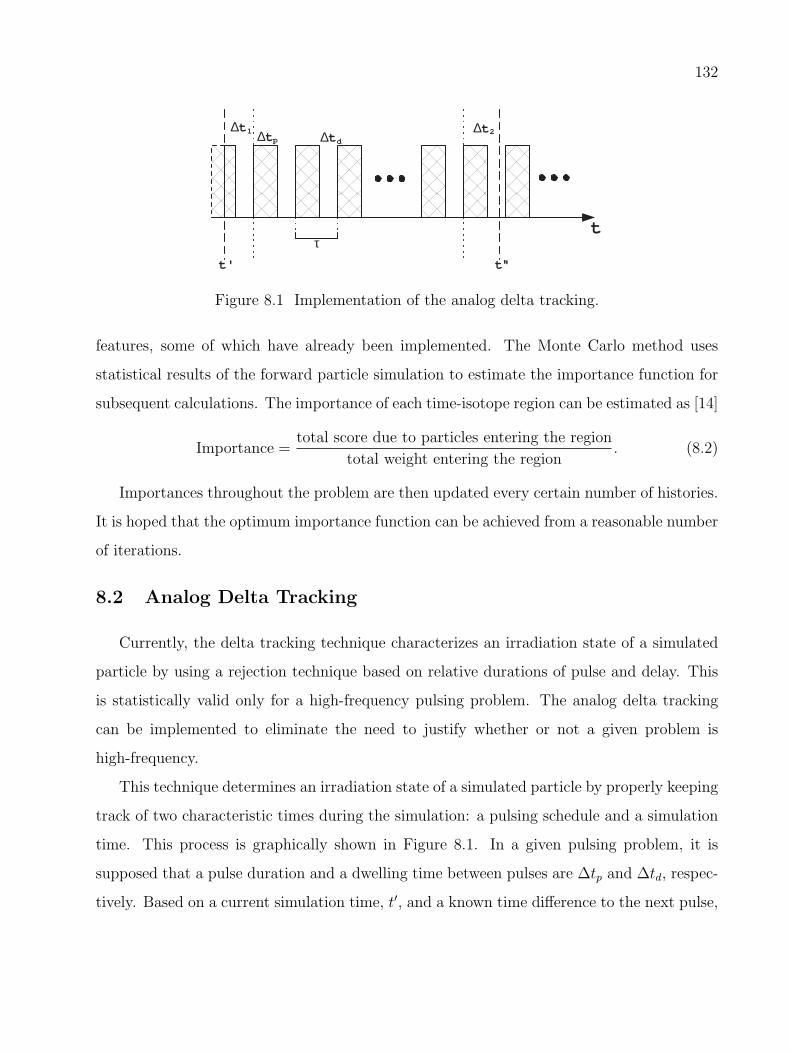
132����������������∆t ∆t

τ

21

t

t' t'

∆t ∆tp d

'

Figure 8.1 Implementation of the analog delta tracking.

features, some of which have already been implemented. The Monte Carlo method uses

statistical results of the forward particle simulation to estimate the importance function for

subsequent calculations. The importance of each time-isotope region can be estimated as [14]

Importance =total score due to particles entering the region

total weight entering the region. (8.2)

Importances throughout the problem are then updated every certain number of histories.

It is hoped that the optimum importance function can be achieved from a reasonable number

of iterations.

8.2 Analog Delta Tracking

Currently, the delta tracking technique characterizes an irradiation state of a simulated

particle by using a rejection technique based on relative durations of pulse and delay. This

is statistically valid only for a high-frequency pulsing problem. The analog delta tracking

can be implemented to eliminate the need to justify whether or not a given problem is

high-frequency.

This technique determines an irradiation state of a simulated particle by properly keeping

track of two characteristic times during the simulation: a pulsing schedule and a simulation

time. This process is graphically shown in Figure 8.1. In a given pulsing problem, it is

supposed that a pulse duration and a dwelling time between pulses are ∆tp and ∆td, respec-

tively. Based on a current simulation time, t′, and a known time difference to the next pulse,

133

∆t1, it is always possible to indicate a position in a pulsing period of another simulation

time, t′′. The modulo operation between (t′′ − (t′ + ∆t1)) and τ is used to calculate ∆t2,

which ultimately determines the location of t′′. If ∆t2 is less than ∆tp, t′′ will be in the

pulsing region. It will fall in one of the dwelling times, otherwise.

8.3 Automated ALARA-based AVA

A coupled Monte Carlo-deterministic method or a hybrid method, which has been pur-

sued in the area of neutron transport [32, 33], has motivated a similar approach to promote

efficiency in inventory analysis problem. This approach is to apply an iterative algorithm

starting with the approximation of the overall reaction tree obtained from a deterministic

calculation. The importance of each reaction pathway is evaluated based on the contribution

it may eventually lead to the response metric.

The concept of a hybrid method is experimented when ARIES-CS is being analyzed

(Section 7.3.3). In this sample problem, AVA driven by the initial input from ALARA is

proved to be a promising technique. However, setting up the hybrid simulation is done

manually and requires a great deal of intrinsic code modifications. These issues must be

resolved before the ALARA-based AVA can be available for a production calculation in a

more practical manner. One solution is to develop interfaces within AVA to handle the

output response from ALARA. AVA then processes the imported information into its usable

fashion. After that, other AVA routines are proceeded as usual.

The automated ALARA-based AVA is hoped to provide an automated and efficient way

of defining a set of parameters for several variance reduction techniques.

134

8.4 Research Summary

MCise is a unique activation code that employs a Monte Carlo technique to simulate

transmutation or decay processes of materials in complex systems with a variety of flowing

conditions. The basic concept of this Monte Carlo method enables the code to provide addi-

tional modeling capabilities, for example, a chemical process, an atom sink and a continuous

source. The analog methodology has been successfully implemented and its solutions of

various activation problems have been validated against comparable solutions produced by

a well validated deterministic activation code, ALARA.

In order to improve precision and accuracy of the analog methodology, several variance re-

duction techniques have been developed. Each technique has its own unique implementation

and advantages that determine a type of simulation in which it can be best applied. Every

implemented technique is proved to provide a distinctive improvement on the corresponding

analog model. Using any variance reduction technique typically increases a computing time

per history and therefore creates a concern over the efficiency. The efficiency of any Monte

Carlo simulation is quantitatively measured by a figure of merit. Two types of figure of

merit offer rigorous approaches to monitor the efficiency of the simulations: (1/R2T ) for a

simulation with a target isotope and (1/DkR2T ) for any generic simulation. Both figures of

merit are successfully tested with different types of simulations. Their performances are as

expected.

Adaptive Variance-reduction Adjustment (AVA) is a simple iterative scheme proposed

to automatically adjust parameters for some variance reduction techniques with a goal to

improve a statistical result of a target isotope. The sample problems demonstrate that

AVA achieves the same accuracy and precision as the analog simulation, with a considerably

shorter computing time.

Finally, the proposed methodology is proved to be applicable to performing a transient

isotopic inventory analysis in nuclear systems with mixing and splitting of material flows as

several engineering samples are examined. As many of the future fuel cycle designs tend to

135

involve complex processes including chemical reactions, mixing of flow paths, and sources

and sinks of material, MCise is hoped to become a reliable activation code and a benchmark

for a deterministic approximation in this research area.

136

BIBLIOGRAPHY

[1] P. P. H. Wilson. ALARA: Analytic and Laplacian Adaptive Radioactivity Analysis.PhD thesis, University of Wisconsin–Madison, 1999.

[2] R. F. Burstall. FISPIN – A Computer Code for Nuclide Inventory Calculations, October1979. ND–R–328(R).

[3] R. A. Forrest and J-Ch. Sublet. FISPACT3 – Users Manual, April 1993. AEA/FUS 227.

[4] J. Jung. RACC: Theory and Use of the Radioactivity code RACC. Argonne NationalLaboratory, May 1979. ANL/FPP/TM–122.

[5] M. J. Bell. ORIGEN – The ORNL Isotope Generation and Depletion Code. Oak RidgeNational Laboratory, May 1973. ORNL–4628.

[6] D. L. Henderson and O. Yasar. DKR-ICF: A Radioactivity and Dose Rate CalculationCode Package (Volume 1). Fusion Technology Institute, University of Wisconsin, April1987. UWFDM–714.

[7] T. R. England and et al. CINDER–7: An Interim Report for Users. Los AlamosNational Laboratory, April 1975.

[8] H. Bateman. Proc. cambridge phil. soc., 1910.

[9] N. Metropolis and S. Ulam. The Monte Carlo method. Journal of the AmericanStatistical Association, 44:335–341, 1949.

[10] M. H. Kalos and P. A. Whitlock. Monte Carlo Methods. J.Wiley and Sons, 1986.

[11] J.M. Hammersley and D.C. Handscomb. Monte Carlo Methods. Fletcher & Son Ltd.,1964.

[12] J. F. E. Briesmeister. MCNP – A General Monte Carlo N-Particle Transport Code,Version 4C. Los Alamos National Laboratory, 2000.

[13] Ivan Lux and Laszlo Koblinger. Monte Carlo Particle Transport Methods: Neutronand Photon Calculations. CRC Press, 1991.

137

[14] Thomas E. Booth and John S. Hendricks. Importance estimation in forward MonteCarlo calculations. Nuclear Technology/Fusion, 5:90–100, January 1984.

[15] K. A. Van Riper and et al. Generation of a Monte Carlo variance reduction map from adeterministic transport calculation. Technical report, Los Alamos National Laboratory,1995.

[16] J. Spanier and E. M. Gelbard. Monte Carlo Principles and Neutron Transport Prob-lems. Addison–Wesley Pub. Co., 1969.

[17] F.B. Brown and T.M. Sutton. Monte Carlo Fundamentals. Knolls Atomic PowerLaboratory, 1996.

[18] Marc A. Cooper. An Automated Variance Reduction Method for Global Monte CarloNeutral Particle Transport Problems. PhD thesis, University of Michigan, 1999.

[19] John S. Hendricks. Private communication, 2006.

[20] Thomas E. Booth. Private communication, 2006.

[21] J. F. Latkowski, J. Sanz, and J. L. Vujic. Impact of pulsed irradiation upon neutronactivation calculations for inertial and magnetic fusion energy power plants. FusionTechnology, 30(3):1470–1474, December 1996.

[22] P. W. Glynn and W. Whitt. The asymptotic efficiency of simulation estimators. Oper-ations Research, 40(3), May–June 1992.

[23] John R. Lamarsh. Introduction to Nuclear Engineering. Addison Wesley, 2nd edition,February 1983.

[24] B. B. Cipiti. Fusion transmutation of waste and the role of the in-zinerator in thenuclear fuel cycle. Technical Report SAND2006-3522, Nuclear and Risk Technologies,Sandia National Laboratories, P.O. Box 5800 Albuquerque, NM 87185-0748, June 2006.

[25] L. El-Guebaly, P. Wilson, and D. Paige. Initial activation assessment for aries compactstellarator power plant. Fusion Science & Technology, 47(3):440–444, April 2005.

[26] G. C. Pomraning. Linear Kinetic Theory and Particle Transport in Stochastic Mixtures.World Scientific Publishing Co. Pte. Ltd., 1991.

[27] G. B. Zimmerman. Recent developments in Monte Carlo techniques. Technical ReportUCRL-JC-105616, Lawrence Livermore National Laboratory, 1990.

[28] T. J. Donovan and Y. Danon. Application of Monte Carlo chord-length samplingalgorithms to transport through a two-dimensional binary stochastic mixture. NuclearScience and Engineering, 143:226–239, 2003.

138

[29] L. El-Guebaly. Fusion Technology Institute, Department of Engineering Physics, Uni-versity of Wisconsin-Madison. http://fti.neep.wisc.edu/aries-cs/builds/build.html.

[30] R. E. Alcouffe, F. W. Brinkley, D. R. Marr, R. D. O’Dell, and W. F. Walters.DANTSYS: A Diffusion Accelerated Neutral Particle Transport Code System. LosAlamos National Laboratory, 1995. LA-12969-M.

[31] M. W. Mickael. A fast, automated, semideterministic weight windows generator forMCNP. Nuclear Science and Engineering, 119:34–43, January 1995.

[32] Alireza Haghighat and John C. Wagner. Monte Carlo variance reduction with deter-ministic importance functions. Progress in Nuclear Energy, 42(1):25–53, 2003.

[33] Edward W. Larsen. Hybrid Monte Carlo-deterministic methods for nuclear reactor-related criticality calculatons. Technical Report DE-FG07-00ID13920, Department ofEnergy, 2003.