Karlstads universitet 651 88 Karlstad Tfn 054-700 10 00 Fax 054-700 14 60

Information@kau.se www.kau.se

Fakulteten för hälsa, natur- och teknikvetenskap Miljö- och energisystem

Linus Zimmerman

Utveckling och validering av propellermodell baserat på rörelsemängdskälla för ett

friströmningsfall

Development and validation of momentum source propeller model in open-water conditions

Examensarbete 30 hp Civilingenjör: Energi- och miljöteknik

Juni 2015 Handledare: Kamal Rezk Examinator: Roger Renström

Master Thesis

DEVELOPMENT AND VALIDATION OF MOMENTUM SOURCE PROPELLER MODEL IN OPEN-WATER CONDITIONS Date : 2015-06-23 Author : Linus Zimmerman Reference: Johan Lundberg Adress : Rolls-Royce Hydrodynamic Research Centre P.O Box 1010, S-681 29 Kristinehamn, Sweden

Abstract

Propeller simulation by Computational Fluid Dynamics (CFD) is more and more used in an early design stage of marine propulsion. Rolls-Royce Hydrodynamic Research Centre has long experience with propeller design and analysis through both model testing and numerical simulations, and CFD is today used in a wide range of applications and purposes.

Utilizing a time efficient and simple simulation approach is a valuable strategy, and time against accuracy is a trade off a designer need to do all the time. In this case the study will concern a modelling approach where the propeller is represented by a cylindrical volume with the same diameter and proportions as an actual propeller. This volume, called an actuator disc volume zone is implemented with the propulsive forces as local source terms into the model and thereby provides momentum into the fluid. Work will be concentrated on developing this simulation model and evaluate its performance by comparison with a more complex propeller geometry model.

The purpose of this work is to investigate the result from a simplified propeller model in regard to the induced velocity field for a propeller operating in a homogeneous inflow field. Analysis of the induced velocity profile is an important step in the design process of propeller-rudder configuration and a computationally efficient method in doing this is highly desirable.

Results from the simulations show that the modelling approach enables simple employment of different propeller types and improves computational efficiency with a third of required time amount compared to the complex propeller model. The induced velocity profiles also demonstrate a relatively accurate behaviour and the model provide useful tools in altering their appearance. Further work need to be considered in optimizing the discretization method and thereby possibly improve solution efficiency, together with examining of a non-uniform inflow velocity condition inspired by the wake created behind a ship hull.

Sammanfattning

Propellersimulering genom Computational Fluid Dynamics (CFD) används mer och mer i ett tidigt designstadium gällande fartygs framdrift. Rolls-Royce Hydrodynamic Research Centre har lång erfarenhet av propellerdesign och analysarbete genom både modelltester och numerisk simulering, och CFD används idag för ett flertal olika tillämpningar och syften. Att utnyttja en tidseffektiv och enkel simuleringsmetod är en betydelsefull strategi och tid gentemot noggrannhet är en avvägning som designers alltid måste göra. I detta fall kommer en förenklad modelleringsprincip studeras där propellern representeras av en cylindrisk volym med samma diameter och proportioner som den faktiska propellern. Denna volym, kallad en aktuatordisk-volym implementeras med framdrivningskrafterna genom inmatning av lokala källtermer i modellen och överför på så vis rörelsemängd till fluiden. Arbetet har fokuserats på utveckling av denna simuleringsmodell och att utvärdera dess prestanda genom jämförelse mot en geometriskt mer komplex propellermodell. Syftet med detta arbete är att undersöka resultat från en förenklad propellermodell med avseende på inducerat hastighetsfält för en propeller som verkar i ett homogent inflödesfält. Analys av den inducerade hastighetsprofilen är ett viktigt steg i designprocessen för propeller-roder-konfiguration och en beräkningseffektiv metod för att uppnå detta är mycket önskvärd. Resultat från simuleringarna visar att modelleringsprincipen möjliggör enkel användning av olika propellertyper och förbättrar beräkningseffektiviteten med en tredjedel av tidsåtgången som krävs för den komplexa propellermodellen. Inducerade hastighetsprofiler visar även på relativt god överensstämmelse och modellen erbjuder användbara verktyg för att variera dess utseende. Fortsatt arbete bör övervägas för att optimera diskretiseringsmetod och på så vis även möjliggöra förbättring av lösningstiden, tillsammans med undersökning av icke-uniformt inflödesvillkor inspirerat av strömningen som skapas bakom en fartygskropp.

Foreword

The work in this master thesis is the result of my last semester at the Energy and Environmental Engineering programme at Karlstad University. It has been written in collaboration with Rolls-Royce Hydrodynamic Research Centre in Kristinehamn, to whom I would like to extend a special thank you. My warmest thanks also goes to Johan Lundberg and my mentor Kamal Rezk who both have been an important support and provided helpful guidance along the way. Additionally my appreciations go to friends and family for their encouragement and confidence in me. Detta examensarbete har redovisats muntligt för en i ämnet insatt publik. Arbetet har därefter diskuterats vid ett särskilt seminarium. Författaren av detta arbete har vid seminariet deltagit aktivt som opponent till ett annat examensarbete. Linus Zimmerman Karlstad 2015-06-23

Nomenclature

Symbol Unit Description

D m Propeller diameter

J - Number of advance

g m/s2 Gravitational acceleration

KQ or KQ - Torque coefficient

KT or KT - Thrust coefficient

n r/s Propeller rate of revolutions

P m Propeller pitch (at 0.7R)

p Pa Pressure

Q Nm Propeller torque

r m Intermediate blade radius

R m Propeller radius

r/R - Non-dimensional blade radius

Re - Reynolds number

T N Propeller thrust

VA m/s Speed of advance

Vf m/s Free-stream velocity

ηo - Propeller efficiency, open water

ρ kg/m3 Density of water

y+ - Non-dimensional wall distance

u, v, w m/s Velocity components

U m/s Mean velocity (u-component)

u’ m/s Fluctuating velocity (u-component)

uτ m/s Friction velocity

t s Time

x, y, z - Cartesian coordinates

ycc m Wall distance to first Cell centre

µ Pa s Dynamic viscosity

∇ - Divergence operator

Contents 1   Introduction .......................................................................................................... 1   2   Background and theory ....................................................................................... 3  

2.1   Earlier work ...................................................................................................... 3  2.2   Propeller Testing .............................................................................................. 5  

2.2.1   Scale effects ............................................................................................... 5  2.3   CFD .................................................................................................................. 6  

2.3.1   Discretization .............................................................................................. 7  2.3.2   Stationary & moving reference frame simulation ........................................ 8  

2.4   Governing equations ........................................................................................ 8  2.4.1   Continuity equation ..................................................................................... 8  2.4.2   Momentum equation ................................................................................... 9  2.4.3   The Navier-Stokes equations ..................................................................... 9  

2.5   Turbulence and modelling ................................................................................ 9  2.5.1   Boundary layer ......................................................................................... 10  2.5.2   y+ ............................................................................................................. 10  2.5.3   Shear Stress Transport k-ω ..................................................................... 11  

3   Method ................................................................................................................. 12  

3.1   Propeller reference ......................................................................................... 12  3.1.1   Model data ................................................................................................ 13  

3.2   ADM ............................................................................................................... 14  3.2.1   User-Defined Functions and Scheme macro ........................................... 14  

3.3   Modelling of geometry for ADM ...................................................................... 15  3.3.1   Meshing .................................................................................................... 16  

3.4   MRF-model ..................................................................................................... 18  3.4.1   Radial distribution of KT and KQ ................................................................ 19  

3.5   Non-uniform inflow condition .......................................................................... 21  3.6   Convergence criteria ...................................................................................... 21  3.7   Simulation cases ............................................................................................ 22  

3.7.1   Reference case and set up ...................................................................... 22  3.7.2   Mesh sensitivity ........................................................................................ 22  3.7.3   Comparison of ADM with MRF-model ...................................................... 23  3.7.4   Radial distribution ..................................................................................... 23  3.7.5   Non-uniform inflow (porous media zone) ................................................. 24  

4   Results ................................................................................................................ 25  

4.1   Reference case .............................................................................................. 25  4.2   Mesh sensitivity .............................................................................................. 26  4.3   Comparison ADM/MRF .................................................................................. 28  

4.3.1   Operating condition J=0,675 .................................................................... 28  4.3.2   Operating condition J=0,975 .................................................................... 30  4.3.3   Solving efficiency and propeller characteristics ........................................ 30  

4.4   Radial distribution ........................................................................................... 31  4.5   Non-uniform inflow ......................................................................................... 33  

5   Discussion .......................................................................................................... 34  6   Conclusions ........................................................................................................ 37   7   List of References .............................................................................................. 38

1

1 Introduction

Propeller simulation by Computational Fluid Dynamics (CFD) is more and more used in an early design stage of marine propulsion. Rolls-Royce Hydrodynamic Research Centre (RRHRC) has long experience with propeller design and analysis through both model testing and numerical simulations, and CFD is today used in a wide range of applications and purposes. Everything from detailed investigation of the propeller blades to the ship hull interaction is made. While experimental model tests have been the traditionally most common approach the development of computing power has enabled a transition towards numerical methods. There are several advantages with this technique and essential is of course the possible savings in both cost and time, as well as easy modification of design parameters and so on. The most time consuming CFD methods simulate the true rotation of the propeller relative the hull, rudder and so forth. A typical time step and angular motion of the propeller is 1-2 degrees and simulation times, depending on the computational resource, are in extreme cases days.(Benini 2004 ; Rolls-Royce 2015) Utilizing a time efficient and simple simulation approach is therefore a valuable strategy, and time against accuracy is a trade off a designer need to do all the time. In this case the study will concern a modelling approach where the propeller is represented by a cylindrical volume with the same diameter and proportions as an actual propeller. This volume, called an actuator disc volume zone (ADZ), is subjected to a velocity-averaging inflow field located upstream of the ADZ and the propulsive forces are applied as local source terms into the model. Work will be concentrated on developing this simulation model and evaluate its performance by comparison with a more complex propeller geometry model. The actuator disc method has been extensively applied and tested in the past for the analysis of propeller-rudder interaction, as well as of the prediction of hull resistance and propulsive efficiency of different ship typologies and configurations (Durante et al. 2013 ; Windén et al. 2014). The theory behind this concept is either known as the Rankine-Froude momentum theory or the general momentum theory of propellers, and can be described as a propeller having an infinite number of blades. The disc is located in the propeller plane and is considered to absorb the engines total power amount and dissipate it into the fluid by causing a pressure jump across the two faces of the disc (Carlton 2007). This axial force is termed as thrust and provides the forward motion of a boat or vessel. Implemented into the simulation model is also a rotational force, denoted torque, which generates a swirl of the water behind the propeller disc. This simplified propeller simulation approach can be used in several applications, for instance rudder design studies, propeller pod or nozzle design work, ship hull simulations and ship hull self propulsion. The main driving force is to enable a fast and flexible simulation model as a supplement to the work in an early design stage. Computational cost and solution times are key factors when many different design parameters need to be studied and evaluated. The purpose of this thesis is to investigate simulation results in regard to induced velocity field downstream of the propeller, using a simplified propeller model operating in a homogeneous inflow field. Analysis of the induced velocity profile is an important step in the design process of propeller-rudder configuration. The aim is to implement a fast simulation model that imitates a typical fluid flow scenario and to

2

assess its performance. Possible further development will be considered as to enable a non-uniform inflow velocity field inspired by the wake created behind a ship hull. Simulations are performed in the CFD software ANSYS Fluent and the modelling process consists of setting up the geometry and fluid domain, including the necessary boundaries to be able to couple with momentum source equations. Furthermore, results will be examined for variations in the discretization and specific input parameters that may influence the induced velocity profile downstream of the propeller disc.

3

2 Background and theory

Computational Fluid Dynamics as well as marine propulsion are complex scientific fields of study and rely on numerous years of research and development work. The chapter below is therefore designated for some basic theory and fundamentals that play a vital part in understanding of the work done in this thesis. Initially some results from literature are presented.

2.1 Earlier work

Gao et al. (2012) has published an article with calculations of propeller-induced velocity through different methods of simulation using Reynolds-Averaged Navier-Stokes (RANS) and momentum theory. The aim is to study hull-propeller interaction and ship self-propulsion, and the authors describe two methods available for modelling of propellers with this purpose; namely the actuator disc (AD) approach or RANS simulation in which the propeller is meshed geometrically. Discussion is held regarding the difficult elements of a body force method (or AD method) in calculation of the induced propeller velocity, which is therefore obtained from potential flow approaches (excluding viscous effects). A full geometry RANS simulation does not have this problem though is instead much more dependent on large computational resources. The computed results show underestimated values in the acceleration of axial velocity and overestimation of the rotational cross flow, which according to Gao et al (2012) may be the subject of used turbulence model. Induced velocities obtained with RANS calculations were consistent with experimental data, however were they significantly overestimated by the momentum theory. In the work of Durante et al. (2013) three different simplified hydrodynamic models are tested based upon theories of Nakatake, Theodorsen and Sears. These models are applied to predict thrust and torque produced by a marine propeller working within an axial inhomogeneous inflow and the results are then validated through Boundary Element Method (BEM) hydrodynamics. The Nakatake model is described by a continuum disc representing the propeller system and based upon open-water performance and potential theory, whereas Theodorsen and Sears depends on propeller loads obtained as radial integration of the sectional loads given by the unsteady airfoil theories. Numerical results show a comparison between these approaches, however display the Sears computations over-predicted signal peaks and Nakatake results a worsening with higher frequencies. The authors summarizes the investigations done throughout the paper with recommending above mentioned theories as appealing, fast, hydrodynamic models for analysis or CFD applications directed at studying hull-propeller configurations in off-design conditions. For the sake of studying propeller-rudder interaction Phillips et al. (2010) examines three different body force propeller methods, i.e. actuator discs. The numerical results are compared with wind tunnel experiments for validation and the body force models to be implemented with RANS simulation are;

• uniform thrust distribution with no torque (an actuator disc applied over a finite thickness)

• radial distribution of thrust and torque proposed by Hough and Ordway (1965), hereby denoted HO

4

• Body Element Momentum Theory (BEMT) distribution of radial and tangential thrust and torque magnitude.

The related methods in the article use the flow-integrated effects of the propeller that generates an accelerated and swirled initial flow onto the rudder. The calculations performed can be considered ‘steady’ by removing the influence of the unsteady propeller flow as long as radial variation and axial momentum produced by the propeller are included. Both the RANS-HO and RANS-BEMT models are pointed out as suitable methods for propeller-rudder analysis, although the HO approach fails to capture the effect of the rudder onto the propeller. The approach with uniform thrust distribution achieves adequate rudder lift estimation however does not predict the rudder drag, and therefore this method is not recommended. Because prescribed torque and thrust distributions concerns an infinitely bladed propeller the authors conclude that a low blade area ratio propeller is not suitable according to the radial distribution of source terms.(Phillips et al. 2010) Greco et al. (2014) perform studies based on a BEM and applied to marine propellers in open water conditions. Drawbacks and capabilities of this method for analysis of propeller hydrodynamics in uniform onset flow are examined and compared with experimental data and RANS simulations. The numerical results confirm that propeller thrust and torque for a wide range of operating conditions is accurately captured. BEM functions correctly with the trailing wake surface in terms of pitch distribution, slipstream contraction and tip-vortices location, where agreement with computations through RANS and the experimental data is sufficient. A worsening of BEM results were shown beneath the design working point, however was this phenomenon not surprising regarding to the complexity of the wake according to the authors. The conclusion from this article is that a BEM hydrodynamic approach is appropriate for analysis of marine propellers and the study of configurations with significant wake-body interactions. The influence of grid type and turbulence model on numerical predictions of propeller performances is analysed in an article by Morgut and Nobile (2012). The meshing methods used are hexa-structured and hybrid-unstructured with similar levels of accuracy and similar requirements of iterations and computational time, which meant a much finer spatial resolution was needed for the hybrid mesh. The two turbulence models used were the Shear Stress Transport (SST) and Baseline-Reynolds Stress Model (BSL-RSM) where the latter is more computationally demanding. The tests were carried out using two different model scale propellers, comparing the global field values of thrust and torque coefficients as well as local values measured in the propeller wake. The results showed that hexa-structured mesh is preferable because it is less diffusive concerning the local flow field, even though this requires more effort when generating the mesh. The two turbulence models impact the numerical simulations similarly with only slightly more accurate predictions for the BSL-RSM when comparing to experimental results. The conclusion from this study is that regarding open water performance the SST model might be a more effective choice since it compels less computational resources.

5

2.2 Propeller Testing

To determine a propellers properties and performance during different operating conditions several types of model testing is conducted. Measurements in an undisturbed fluid stream is known as open water testing, where the forces and moments of a propeller working in varying speed of advance can be defined. For scaling purposes there are some aspects that need to be considered when modelling propellers both in a numerical and actual testing environment. These are often referred to as general open water characteristics when describing the forces and moments acting on the propeller, while operating in a uniform fluid stream. The characteristics are expressed in a series of non-dimensional coefficients, general for a specific geometric configuration, and defined in the equations (1-3) below.(Carlton 2007 ; Tornblad 1990)

• Thrust coefficient, KT (1)

• Torque coefficient, KQ (2)

• Advance coefficient, J

(3)

The thrust coefficient is based on the actual thrust provided to the propeller T, density of water 𝜌, number of revolutions n and the diameter of the propeller D. In a similar manner the torque coefficient is described, however with the difference of applied torque on the propeller shaft Q. The advance coefficient J can be explained as a non-dimensional velocity and depends on VA, which is the speed of advance. VA can further be described as the velocity of the moving vessel or in open water conditions rather the free stream velocity in which the propeller is currently working.

2.2.1 Scale effects

A model scale propeller has generally a diameter between 200 to 300 mm, smaller than this will likely affect performance due to the build up of boundary layer, which is dependent on Reynolds number (Carlton 2007). See equation (4), including fluid density ρ, mean velocity v, characteristic length L and dynamic viscosity µ. 𝑅𝑒 =

𝜌 ∙ 𝜈 ∙ 𝐿𝜇 (4)

Inertial forces govern flows with large Reynolds number while a low Reynolds number indicates that viscous effects dominate. This dimensionless quantity defined

42 DnTKT ⋅⋅

=ρ

52 DnQKQ ⋅⋅

=ρ

DnV

J A

⋅=

6

above can be used to predict related flow patterns in separate fluid flow cases.(Munson et al. 2013 ; Tritton 1977)

2.3 CFD

Computational fluid dynamics, CFD, utilizes the governing partial differential equations (PDEs) of fluid motion with the method of discretized algebraic equations that approximate these PDEs. The equations are then numerically solved and can be applicable to a wide variety of flow problems. This can be simplified as the simulation and analysis of fluid flows, thereby including heat and mass transfer and chemical reactions and much more, using computational resources.(Keon-Je & Shin-Hyoung 1995 ; Rhee & Joshi 2006) The development of CFD primarily originated in aerospace industry as a research tool, this is still the case however also with further use as a design tool for several engineering purposes. Important advantages with this technique are the possibility of savings in both cost and time for industries using CFD as a tool that complements the experimental and theoretical work in fluid dynamics.(Munson et al. 2013) A general procedure describing the workflow of CFD simulations consist of the three main parts pre-process, solving and post-processing.

• Pre-process During pre-processing a series of operations are performed in defining the prerequisites for a model before it can be computationally solved. This includes setting up of geometry, dividing the fluid domain into discrete cells (meshing) and defining the physical modelling e.g. equations of motion or radiation. Definition and specification of certain boundary conditions are also needed; this involves applying fluid behaviour and properties at the boundaries of a problem.(Rhee & Joshi 2006) • Solving A commonly used numerical solving technique within CFD is the finite volume method (FVM), which furthermore acts as the approach used in this study. This method solves the governing partial differential equations over a discrete control volume through a reorganization of the equations in a conservative form. Conservation of the fluxes throughout a specific control volume is thereby guaranteed in this discretization process. FVM has an advantage from other numerical methods in the memory usage and solution speed particularly concerning large problems, turbulent flows with high Reynolds numbers and so on.(Morgut & Nobile 2012) There are also different types of solvers to be employed, for example pressure-based or density-based. In this work a pressure-based solver is used, concerning how solving is executed through pressure equations derived from the momentum and continuity equations (described in section 2.4 below). Further a segregated or coupled solution algorithm represents how velocity components and pressure-correction continuity equations are solved sequentially or simultaneously. The

7

coupled algorithm with simultaneous calculations improves the time rate towards reaching convergence, however with an increased memory requirement. • Post-process The post-processing is the stage of analysing the simulation results through visualization or other types of data processing. Often by plots describing velocity or pressure contours, calculation of specific values in the flow field and much more.

2.3.1 Discretization

To be able to numerically solve the algebraic equations require dividing the computational domain into discrete points where the continuous flow field then can be calculated, often as velocity or pressure as a function of space and time. The discretization is known as a grid or mesh and contains of various geometrically formed elements connected to one another. Classification of mesh type is often done by the means of connectivity or element shapes used. Regarding connectivity this includes structured, unstructured or a hybrid mesh. Structured implies a regular connectivity with elements of rectangles or triangles (in 2D). Unstructured depends on irregular connections with various and unevenly shaped elements, while the hybrid mesh are a mix up of the two preceding. Element-based classification concerns the dimensions or types present; either for meshes generated in 2D or 3D. For a 3-dimensional case the most commonly used elements are hexahedra or tetrahedral. See figure 1 for examples of 3D mesh elements.(Munson et al. 2013 ; Keon-Je & Shin-Hyoung 1995)

Figure 1. Various geometrically shaped 3D elements (Wikimedia commons 2015)

8

Solution accuracy is dependent on the number of cells in a mesh where both a higher number and the generation method is affecting, as well as the number of order in the discretization scheme applied (regarding the solving of pressure/velocity equations). Time requirement is also directly correlated to resolution rate because the amount of iterations increase with each mesh cell added.(ANSYS Theory Guide 2015)

2.3.2 Stationary & moving reference frame simulation

A stationary or steady-state solution performs a mass and energy balance of a process in an equilibrium state. This means no change in respect to time and therefore avoids additional transient terms usually leading to easier convergence behaviour (Veersteg & Malalasekera 2007). Using a moving reference frame (MRF) gives an opportunity to solve a problem that is unsteady in the stationary (or inertial) frame steady with respect to the moving frame. A flow being subjected to a constant rotational speed, where the frame is steadily moving, is therefore available as a steady-state solution due to a transformation of the equations of fluid motion.(ANSYS Theory Guide 2015)

2.4 Governing equations

The motion of a fluid is governed by a set of nonlinear partial differential equations and is a highly complex matter. In order to give an overview of the physics regarding fluid motion follows a chapter with brief description of these equations.

2.4.1 Continuity equation

The adoption of fluids regarded as continuous is often described as the conservation of mass principle, or the continuity equation, which is presented in equation (5) and (7) below. This means that for a certain control volume the mass of the system remains constant as it moves through the flow field.

∇ ∙ 𝒖 =𝜕𝑢𝜕𝑥 +

𝜕𝑣𝜕𝑦 +

𝜕𝑤𝜕𝑧 = 0 (5)

For a stationary and incompressible fluid case the equation simplifies to what is seen above, written both in vector notation and Cartesian coordinates. 𝛻 is called the divergence operator and u(u,v,w) is the velocity vector regarding the flow in x, y and z-directions. ∂ρ

∂t + ∇ ∙ 𝜌𝒖 = 0 (6)

An unsteady, compressible fluid flow case can be expressed in short hand as equation (6) where 𝜌 is fluid density and 𝑡 time.

9

2.4.2 Momentum equation

The momentum equation refers to Newton’s second law of physics stating that the rate of change of momentum of a fluid particle is the same as the combined forces acting on the specific particle (F=ma). Two different types of forces can be distinguished; surface forces and body forces. These include pressure and viscosity, gravity or centrifugal force and so on. The contributions of surface forces are often denoted as separate terms in the momentum equation while the effects of body forces are included as source terms.(Veersteg & Malalasekera 2007) Considering a small control volume, or fluid element, the state of stress of this element is defined by the pressure and viscous stress components acting in all directions (3-dimensionally), and can be derived from a force balance over the control volume. The pressure component is directed normally to the boundary and normal stress and viscosity include the shearing stresses acting on all sides of the fluid element.

2.4.3 The Navier-Stokes equations

Combining the equations of motion and conservation of mass principle, the continuity equation, provides the renowned Navier-Stokes equations in which fluid flow is mathematically described. The ones who were responsible for this formulation are L. M. H. Navier and Sir G. G. Stokes, the French mathematician respectively mechanic from England operating during the 18th and 19th century. Because of the complexity of the equations there are no exact solution available to this date, in except for the simplest case possible where good agreement has been shown compared to experimental results.(Munson et al. 2013)

(7)

The differential equation presented above, equation (7), represents the fluid flow solely in the x-direction. To the left is the inertial term including velocity vector u(u,v,w), fluid density ρ and time t. On the right hand side body force-, pressure- and viscous terms can be seen with additional variables of gravity gx, pressure p and dynamic viscosity µ.

2.5 Turbulence and modelling

Turbulence is the state of chaotic and irregular fluid flow behaviour often leading to three-dimensional build-up of vortexes or eddies. This phenomenon is when present generally dominating all other fluid flow situations and increases the mixing, heat transfer and energy dissipation severely. Turbulence can be referred to as an eddying motion in which the local vorticity give rise to this specific flow pattern.

𝜌 !𝜕𝑢𝜕𝑡 + 𝑢

𝜕𝑢𝜕𝑥 + 𝑣

𝜕𝑢𝜕𝑦 + 𝑤

𝜕𝑢𝜕𝑧!!!!!!!!!!!!!!!!!!!!

= 𝜌𝑔!!  −  𝜕𝑝𝜕𝑥!  +  𝜇 !

𝜕!𝑢𝜕𝑥! +

𝜕!𝑢𝜕𝑦! +

𝜕!𝑢𝜕𝑧!!!!!!!!!!!!!!!!!

 

Viscous terms Body force term

Pressure term Inertial terms

10

Eddies appear in a wide range of sizes and the different compositions interact with each other and gain energy from the mean flow.(Tritton 1977) For many engineering purposes turbulent flow situations are present and can often be observed from when the Reynolds number in laminar flows is increased. Calculation of turbulence however presents a serious challenge, as been discussed earlier with the complexity of the Navier-Stokes equations in mind. For an exact solution this means resolving of the whole range of spatial and temporal turbulence scales and this technique is termed direct numerical simulation (DNS). The computational cost of DNS is excessive and in a practical manner impossible for industrial applications as of today.(Veersteg & Malalasekera 2007) To provide an approximation of turbulent flow Reynolds-Averaged Navier-Stokes equations (RANS equations) are used. This is a time-averaged equation where instantaneous quantities are decomposed into its time-averaged and fluctuating quantity. As described in equation (8) the time dependent velocity u is expressed by a mean velocity U and the added fluctuation u’, also dependent on time t. 𝑢 𝑡 = 𝑈 + 𝑢′(𝑡) (8) The technique of RANS-modelling is extensively used and serves as a practical way of solving turbulent fluid flow scenarios.

2.5.1 Boundary layer

When a fluid is flowing past some kind of object there are certain physical phenomenon that describes the velocity layer in the immediate vicinity of the boundary. Considering a flat plate, the flow against the surface is decelerated because of friction (the no-slip condition) and above this is a laminar region established where the fluid particles are composed in a smooth and well-ordered fashion. Farther away from the surface a flow transition occurs where laminar and turbulent effects becomes mixed, with a rise of the Reynolds number along this transitional region. Lastly the outer part of the boundary layer is fully turbulent resulting in the chaotic and random eddies mentioned in the preceding section.(Munson et al. 2013)

2.5.2 y+

A standard feature used in a meshing procedure is the non-dimensional wall distance y+, which relates to the near-wall mesh resolution and determination if the flow is laminar or turbulent in this region. See equation (9) where uτ is the friction velocity, ycc cell height, µ dynamic viscosity and ρ fluid density.

(9)

µρ τ ccyu

y⋅⋅

=+

11

This wall distance can be estimated using a relationship where friction velocity, uτ, divided by the relative fluid speed (e.g. free stream velocity) should be equivalent to 0,035 – 0,050 (Tritton 1977).

2.5.3 Shear Stress Transport k-ω

Specific turbulence models commonly used are the so-called two-equation models, in which two added transport equations describing turbulent flow properties are included. These transport variables are often represented by the kinetic energy k and turbulent dissipation ε or specific diffusion ω. The turbulence models k-ε and k-ω has become an industrial standard and are implemented for many different engineering purposes.(Veersteg & Malalasekera 2007) A development of the equations mentioned above is the shear stress transport k-ω (SST k-ω), which has become an increasingly popular turbulence model. This formulation creates a hybrid model with resolution of the near-wall region by the k-ω model and the fully turbulent flow far from the wall by transformation into the k-ε equations. This combines the best features from both these models and gives it a broader applicability. The near-wall treatment provides solving without additional damping functions and the formulation used in the far field improves robustness, making the SST k-ω a suitable approach with adverse pressure gradients and flow separation behaviour.(Menter 1994)

12

3 Method

As an initial description of the methodology employed in this chapter follows a general overview of each subsection and its contents. Firstly, the propeller design for which simulations are based on is presented, with scaling parameters and dimensions as seen in section 3.1 below. This is continued with data concerning the specific propeller performance working as input of propulsive forces into the Actuator Disc Model (ADM). Thereafter comes an explanation of the technique in implementing momentum source equations into the simulation model and further a definition of necessary boundary conditions needed for coupling with these equations. A modelling chapter follows next, with geometrical set up and description of the computational domain. The meshing procedure is then presented and a reference mesh case is stated. In next section is the model used as validation and comparison demonstrated, the MRF model, with information of the numerical set up and specific modelling approach. Followed by this is the radial distribution of thrust and torque provided as input to ADM, development into a non-uniform inflow scenario and a section regarding certain convergence criteria during simulations. Lastly, a description of studied cases is given in section 3.7 concerning parameters in the reference case set up and the particular conditions being altered in following simulations. The intention has been to qualitatively analyse results in terms of the induced velocity field from the propeller model. Continuing sections in this chapter gives a more thorough description of the work process and methods used in this thesis.

3.1 Propeller reference

Simulations are executed in model scale geometry and concern the characteristics of a five bladed propeller manufactured by Rolls-Royce, mounted on a simplified shaft and hub, as seen in figure 2. This propeller and shaft arrangement was available as a ‘parasolid’ geometry file and imported into the design program where propeller blades were removed and replaced by the actuator disc domain.

13

Model propeller diameter is 0,2543 m compared to the full size measurement of 2,80 m, and the scaling factor corresponds to 0,0908. The simplified shaft and hub arrangement, referred to as “cigar”, has a diameter of 0,790 m. The width of the blade surface in the flow direction (blue z-axis), indicated by a black arrow in the top of figure 2, works as an input of the ADZ thickness and has been estimated to 0,047 m. In the same manner the propeller diameter has been used when modelling size of the AD. The propeller pitch for this specific design is P/D=1,45 at 70% of the propeller radius.

3.1.1 Model data

The propeller performance data used as an input to the ADM are derived from model scale testing in cavitation tunnel T-32 at RRHRC. Experimental open water tests have been performed and the values of thrust and torque during different operating conditions have been measured. By altering the revolution rate or inflow velocity the performance of a propeller is defined, figure 3 shows a representation of open water characteristics. KT and KQ varies with the advance coefficient J and the propulsive efficiency is determined, see equation (10). 𝜂! =  

𝐾!𝐾!

∙𝐽2𝜋 (10)

Figure 2. Propeller model, hub and shaft set up

14

Figure 3. Propeller performance characteristics diagram

3.2 ADM

An existing model structure of the Actuator Disc Model was available through an earlier project on RRHRC, in cooperation with ANSYS Sweden, and forms the basis of the work done in this study. The ADM consists of a C function file (written in the programming language C) and ‘Scheme’ macro file, which include the required momentum source equations and definition of boundaries and necessary conditions for implementing these equations with a geometrical model.

3.2.1 User-Defined Functions and Scheme macro

As a method to enhance solvers standard features, in ANSYS Fluent, a C function file can be dynamically loaded into the program. This is called a User-Defined Function (UDF) and can after interpretation or compilation be used to customize boundary conditions, source terms in Fluent transport equations or adjust computed values on a once-per-iteration basis and so on. A Scheme macro makes it possible to define variables and store these in Fluent, which can thereafter be accessed through the UDF. The specific UDF used in this work compute the local thrust and torque distribution in the AD volume, ADZ, thereby acting as a momentum source contribution into the model. This is enabled through input of the non-dimensional thrust, KT, and torque ,KQ, coefficients described by a polynomial function of the propeller characteristics, see figure 3. The contribution in momentum by these characteristics can be deduced back to the Navier-Stokes equations as adding a local body force term (described as 𝜌𝑔! in equation 7). Polynomial functions of the radial distribution of thrust and torque through out the ADZ are also a required input and are described in section 3.4.1 below. Further a set of boundary conditions needs to be specified in the geometry for coupling with the equations in the UDF, as listed below. These conditions are used as input for the calculation of a momentum source term and will be reconnected to in the following modelling chapter, see figure 5.

KT,  KQ  

J  

KT  

10*KQ  

Ef*iciency  

15

• A shaft/hub entity (or ship hull)  • A volume zone entity for the AD  • A face entity for the AD cylinder side  • A side face entity for AD outflow side  • A face entity for the Circular Inflow Area, CIA (velocity average plane)  

At the CIA boundary an average velocity is detected, computed based on the specific area of placement inside the flow field. This velocity works, together with specified rotational velocity, as the input of operating condition to the AD by defining the advance coefficient J. Regulation of applied thrust and torque into the model is therefore directly correlated to data gathered in the CIA region.

3.3 Modelling of geometry for ADM

The geometry was stated based on a similar body force simulation performed at RRHRC though with another CFD software. The computational domain and mesh followed this template as an initial verification of simulations performed with the ADM. The ADM geometry was created in ANSYS DesignModeler and is based on an actual RRHRC propeller design. Figure 4 gives an overview of the model geometry, with an outer cylinder domain of 2 m in diameter and length 1,5 m. The ADZ is located on the middle of the cigar shaped shaft/hub and upstream (in negative z-direction) is the velocity averaging inflow plane (CIA). The actuator disc calculates thrust and torque depending on the input of velocity from the CIA. Further upstream is the velocity inlet boundary and on the left side the cylinder face zone represents a pressure outlet condition. The outer cylinder surface is defined as a symmetry boundary and the total volume inside the grey cylinder is the actual computational domain.

Figure 4. Overview of geometry set up and computational domain

16

Figure 5 gives a closer view of the shaft, ADZ (green), CIA and to the right inlet velocity boundary. These domains include mentioned face entities for the actuator disc and inflow plane as to compute forces defined in the UDF. The shaft has been cut out of the fluid domain and therefore only leaving its outer surface boundaries where the no-slip condition applies.

Initial simulations where the CIA was placed closer to the ADZ showed significant impact of a suction effect because of the acceleration of water in the actuator disc. This resulted in placement of the velocity-averaging plane 0,450 m upstream (of the ADZ), well away of the suction zone.

3.3.1 Meshing

The general meshing procedure is based on refining the areas of interest and allows coarser elements in the outer domain, which is a well-proven method according to literature (Morgut & Nobile 2012; Philips et al. 2010). This enables containing total cell count on acceptable levels and still maintain high resolving where data analysis is performed. Meshing have been executed using the ANSYS Meshing application and with the default settings of tetrahedron elements, resulting in a hybrid-unstructured mesh type.

AD outflow side

CIA plane

AD side face

Figure 5. ADZ and boundaries for implementation of momentum source terms

17

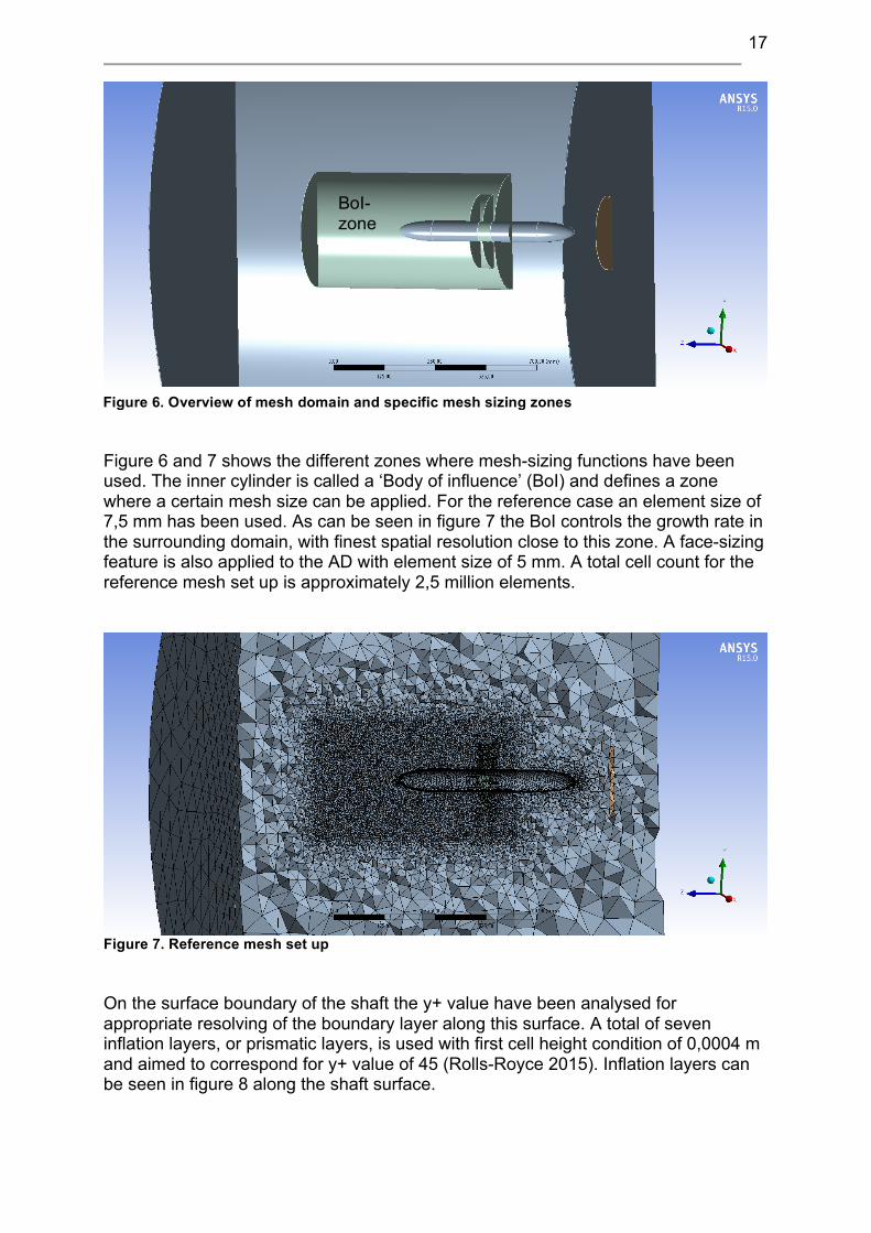
Figure 6 and 7 shows the different zones where mesh-sizing functions have been used. The inner cylinder is called a ‘Body of influence’ (BoI) and defines a zone where a certain mesh size can be applied. For the reference case an element size of 7,5 mm has been used. As can be seen in figure 7 the BoI controls the growth rate in the surrounding domain, with finest spatial resolution close to this zone. A face-sizing feature is also applied to the AD with element size of 5 mm. A total cell count for the reference mesh set up is approximately 2,5 million elements.

Figure 7. Reference mesh set up On the surface boundary of the shaft the y+ value have been analysed for appropriate resolving of the boundary layer along this surface. A total of seven inflation layers, or prismatic layers, is used with first cell height condition of 0,0004 m and aimed to correspond for y+ value of 45 (Rolls-Royce 2015). Inflation layers can be seen in figure 8 along the shaft surface.

BoI-zone

Figure 6. Overview of mesh domain and specific mesh sizing zones

18

3.4 MRF-model

As a validation of the ADM performance and accuracy, the model was compared to a more complex and higher fidelity simulation. This simulation is based on the same propeller case and utilizes a moving reference frame rotating around the propeller. The two modelling approaches, MRF and ADM, have been set up with equal operating conditions and matched to fit propeller performance data. The results from MRF simulations are however entirely numerical and pose a difference to these from the ADM, based on experimental model scale testing. Numerical and experimental differences in open water conditions are well documented in literature and should normally be within 2-5% for a reliable result, when considering the performance characteristics. However are deviations up to 12% reported in some of the studied cases.(Andersen et al. 2014 ; Vyšohlíd & Mahesh 2007 ; Sánchez-Caja 2014) To manage simulations with the numerically complex model (MRF) the RRHRCs in-house developed design program PropCalc were used. This is a highly automated application where a database with design information and specification of operating conditions etc. can be coupled with different calculation operations to efficiently retrieve data of propeller performance and much more. An automated and parametric RRHRC developed mesh tool is integrated and linked to the Fluent solver making it available with CFD simulation dependent on simple user-input of basal design conditions. Figure 9 describes the output of mesh from PropCalc. The MRF model is based on a method where only one of the five propeller blades is modelled using periodic symmetry conditions for the remaining geometry. This lead to lesser computational demand and a mesh consisting of approximately 1,5 million cells, in other words a more time efficient simulation process. The turbulence model used in the MRF simulations is the SST k-ω.

Figure 8. Inflation layers along the shaft surface

19

Figure 9. Overview of MRF mesh (top) and propeller blade & shaft (bottom)

3.4.1 Radial distribution of KT and KQ

A requirement in the Fluent ADM model is an input of radial distribution of the source terms for thrust and torque forces. This data was retrieved from numerical calculations in the design tool PropCalc, and based on lifting surface theory. A lifting surface is explained as an idealized thin 2-D foil section, which is extended into three dimensions and calculated for a steady, incompressible and inviscid fluid flow case (Kerwin 2001). However this data needed to be validated due to the fact that this approach was not ordinary at RRHRC. Therefore analysis of the radial distribution of the forces was performed through earlier MRF simulation results, performed with the propeller of reference by the automated CFD-analysis function in PropCalc. During post processing a single blade was examined, by separating it in ten radially distributed circle sectors as shown in figure 10. For each sector was the hydrodynamic- and viscous pressure integrated with a calculation function within the application CFD-Post, as to acquire local thrust and torque in the blade sections.

20

The integrated forces were plotted as a function over the local radius with the outcome shown in figure 11 and 12, where both PropCalc lifting surface calculations and the MRF simulation are included for comparison. Both thrust and torque are normalized as well as the local radius (local radius r divided by propeller radius R).

Figure 10. Radial sections of propeller blade

0  

0,2  

0,4  

0,6  

0,8  

1  

1,2  

0   0,2   0,4   0,6   0,8   1   1,2  

Normalized  thrust  

Norm.  radius  

KT  -­‐  PropCalc  data  

KT  -­‐  MRF  integrated  

0  

0,2  

0,4  

0,6  

0,8  

1  

1,2  

0   0,2   0,4   0,6   0,8   1   1,2  

Normalized  torque  

Norm.  radius  

KQ  -­‐  PropCalc  data  

KQ  -­‐  MRF  integrated  

Figure 11. Thrust distribution over local propeller radius

Figure 12. Torque distribution over local propeller radius

21

The two procedures describing the radial distribution of forces show good agreement and confirmed that data from the design program, PropCalc, was sufficient. By expressing this distribution through a polynomial function it could thereafter be implemented into the ADM model.

3.5 Non-uniform inflow condition

In an actual propeller case the inflow of water is inhomogeneous due to the wake created by the ship hull (Andersen et al. 2014; Durante et al. 2013; Gaggero et al. 2010). A propeller is therefore exposed to various heavy loads throughout the propeller surface and being able to capture these effects in an early stage of modelling would be preferable. Through creation of an additional body in the geometry set up, placed in front of the AD and velocity-averaging plane, disturbing the inflow field a simulated non-uniform velocity profile is possible. Figure 13 shows the altered set up where CIA has been moved further downstream to fit behind the new geometrical domain. The cylinder disc has a diameter set to 0,6 m, and has been separated into eight sections with the intention to manually control the inflow by applying different permeability.

3.6 Convergence criteria

To reach convergence can be a complex issue where many parameters can be considered important. Residual levels are a key factor however should not only be judged based on the decrease of a specific value; the behaviour can also provide information about the process towards convergence. Good practice is described as continuing with additional 50 iterations as a minimum after residual values dropped sufficient orders of magnitude and stabilized, combined with monitoring relevant integrated quantities such as mass-flow rate or drag force (ANSYS Theory Guide 2015). Several different parameters have been examined through out this study and selected simulations have been carried out with more than 1000 iterations to ensure a reliable solution. An average between 300-400 iterations have been considered sufficient to fulfil above-mentioned criteria.

Figure 13. Non-uniform inflow zone upstream of AD & CIA

22

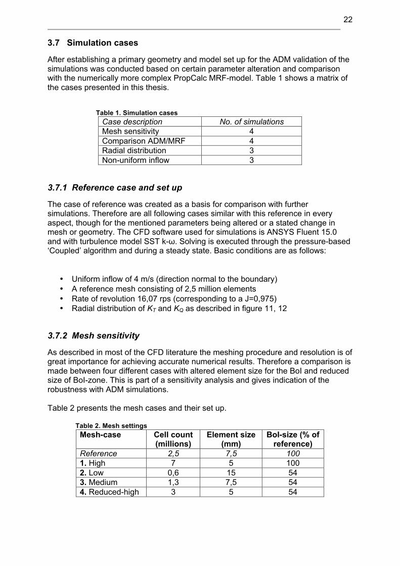
3.7 Simulation cases

After establishing a primary geometry and model set up for the ADM validation of the simulations was conducted based on certain parameter alteration and comparison with the numerically more complex PropCalc MRF-model. Table 1 shows a matrix of the cases presented in this thesis.

Table 1. Simulation cases Case description No. of simulations Mesh sensitivity 4 Comparison ADM/MRF 4 Radial distribution 3 Non-uniform inflow 3

3.7.1 Reference case and set up

The case of reference was created as a basis for comparison with further simulations. Therefore are all following cases similar with this reference in every aspect, though for the mentioned parameters being altered or a stated change in mesh or geometry. The CFD software used for simulations is ANSYS Fluent 15.0 and with turbulence model SST k-ω. Solving is executed through the pressure-based ‘Coupled’ algorithm and during a steady state. Basic conditions are as follows:

• Uniform inflow of 4 m/s (direction normal to the boundary) • A reference mesh consisting of 2,5 million elements • Rate of revolution 16,07 rps (corresponding to a J=0,975) • Radial distribution of KT and KQ as described in figure 11, 12

3.7.2 Mesh sensitivity

As described in most of the CFD literature the meshing procedure and resolution is of great importance for achieving accurate numerical results. Therefore a comparison is made between four different cases with altered element size for the BoI and reduced size of BoI-zone. This is part of a sensitivity analysis and gives indication of the robustness with ADM simulations. Table 2 presents the mesh cases and their set up.

Table 2. Mesh settings Mesh-case Cell count

(millions) Element size

(mm) BoI-size (% of

reference) Reference 2,5 7,5 100 1. High 7 5 100 2. Low 0,6 15 54 3. Medium 1,3 7,5 54 4. Reduced-high 3 5 54

23

3.7.3 Comparison of ADM with MRF-model

The ADM and MRF-model are simulated at two operating conditions, J=0,675 and J=0,975 (as in the reference case). The inlet velocity has been kept constant while the revolution rate was increased from 16,07 to 23,3 rps. This is done as to evaluate the performance during different propulsive load and thereby controlling the ADM consistency. A quantification of time requirement and computational resource between the two numerical methods are estimated, concerning amount of CPU power used and time elapsed in the convergence process.

3.7.4 Radial distribution

As a means of testing the function of a specific ADM input the radial distribution of forces has been examined. This parameter has the ability of influencing the propeller induced velocity profile and may be useful in optimizing the actuator disc method to represent certain propeller geometries. Three simulations with altered radial distribution is considered, where the distributions are made-up and have been created based on extreme cases of radial load at the tip, root and evenly through out the AD radius. Figure 14, 15 and 16 describes the different distributions working as the input of polynomial functions into the UDF and Scheme macro.

0   0,5   1   1,5   Radius   0   0,5   1   1,5   Radius  

0   0,5   1   1,5   Radius  

Figure 14. Tip load (alternative 1) Figure 15. Root load (alternative 2)

Figure 16. Uniform load (alternative 3)

24

The diagrams show representative distributions of thrust and torque forces along the propeller radius, which is why the quantity on the vertical axis has been removed.

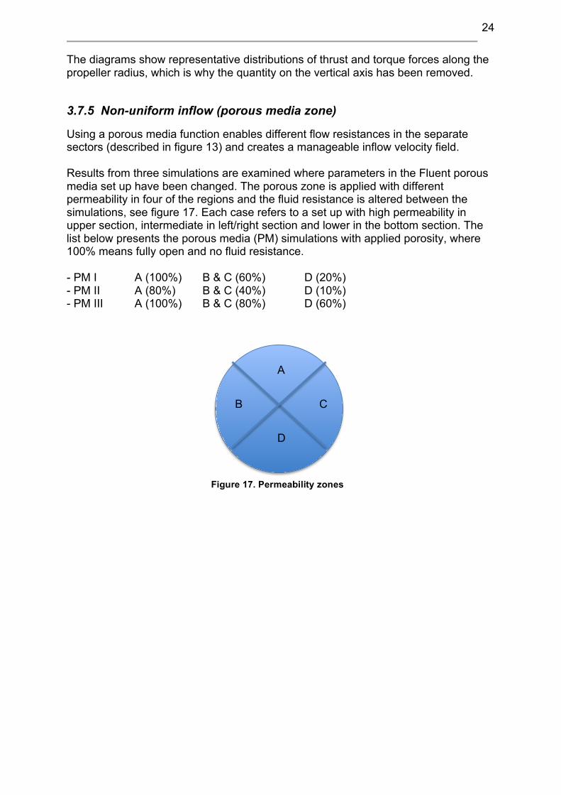
3.7.5 Non-uniform inflow (porous media zone)

Using a porous media function enables different flow resistances in the separate sectors (described in figure 13) and creates a manageable inflow velocity field. Results from three simulations are examined where parameters in the Fluent porous media set up have been changed. The porous zone is applied with different permeability in four of the regions and the fluid resistance is altered between the simulations, see figure 17. Each case refers to a set up with high permeability in upper section, intermediate in left/right section and lower in the bottom section. The list below presents the porous media (PM) simulations with applied porosity, where 100% means fully open and no fluid resistance. - PM I A (100%) B & C (60%) D (20%) - PM II A (80%) B & C (40%) D (10%) - PM III A (100%) B & C (80%) D (60%) A

B

D

C

Figure 17. Permeability zones

25

4 Results

Subsequent section contains results from simulations and the modelling process described in the method chapter. Firstly a brief description of the reference case is presented and then followed by illustration and comparison of remaining cases. The simulation results are presented as contour plots of the velocity field in cross-sections showing axial and tangential velocity components. Analysis of data in Matlab has also been performed through 2D graphs of the velocity field downstream of AD, with the intention to better quantify differences between separate simulations.

4.1 Reference case

Figure 18 shows an overview of the axial flow where the acceleration of water is indicated by the red/orange area. In front of the hub stagnation occur and in the stern a flow separation is noticeable. The solution was considered converged after approximately 300 iterations, and to reassure this a continuing with the double amount of iterations showed no noticeable change in residuals or drag force monitor.

The dashed black line represents the area where data of the axial and tangential velocity components have been gathered. One propeller radius equals 0,12715 m and the analysis provide information of the induced velocity profile from the shaft surface to the free stream region.

1 propeller radius downstream

Figure 18. Reference case simulation showing axial velocity

26

4.2 Mesh sensitivity

The analysis of different mesh resolution shows a variance in the induced velocity field behind the AD. Figure 19 represents the low, medium and reference cases in the same order from top to bottom, as to visualize how different BoI size and resolution controls the growth rate of surrounding elements. The diffusion outside the refinement zone is clearly demonstrated in the low mesh case and with higher resolution the induced velocity field becomes better preserved further downstream. For a better representation of the induced velocity field for the actuator disc (or propeller) data from one propeller radius distance downstream of the AD has been analysed, as described in previous section 4.1. Figure 20 shows 2D plots of the axial velocity field for each mesh resolution, compared to the reference case. The velocity has been normalized with the free stream velocity (Vf = 4 m/s). The upward distance, normal to the flow direction, has been normalized with the propeller radius (local radius r divided by propeller radius R). The maximum velocity fluctuates with less than 10% between mesh case 3 ‘medium’ and nr. 1 ‘high’ resolution simulations, and reference case is most contiguous to the

Figure 19. Mesh cases low, medium and reference showing axial velocity

27

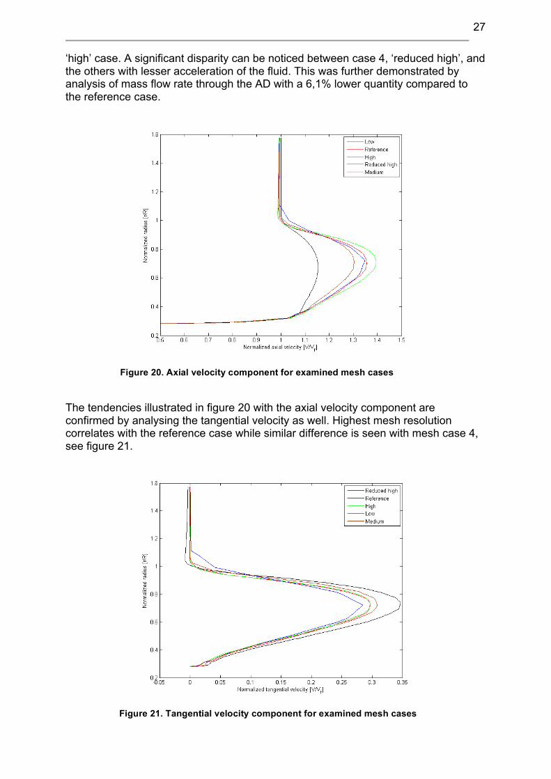
‘high’ case. A significant disparity can be noticed between case 4, ‘reduced high’, and the others with lesser acceleration of the fluid. This was further demonstrated by analysis of mass flow rate through the AD with a 6,1% lower quantity compared to the reference case. The tendencies illustrated in figure 20 with the axial velocity component are confirmed by analysing the tangential velocity as well. Highest mesh resolution correlates with the reference case while similar difference is seen with mesh case 4, see figure 21.

Figure 20. Axial velocity component for examined mesh cases

Figure 21. Tangential velocity component for examined mesh cases

28

A converged solution was reached after approximately one hour in the reference case while highest resolution, mesh nr. 1, amounted more than three times this number.

4.3 Comparison ADM/MRF

The comparison between ADM and MRF simulations are presented for two different operating conditions, where the revolution rate has been altered.

4.3.1 Operating condition J=0,675

With a higher revolution rate, n=23,3 rps, the thrust and torque transferred to the fluid is increased, as described by the propeller performance diagram. Figure 22 presents the axial flow of the ADM compared to MRF-model. The ADM shows a rather uniform acceleration of water while the pulsation effect from the propeller blade can be seen in the lower half of the figure. Wake profiles downstream of the shaft differs between the two numerical methods, with a larger separation of flow related to the actuator disc model and indicated by the black circle in the figure.

Studying axial velocities in a cross-section downstream from AD/propeller gives the appearance as figure 23. ADM reveals a uniform distribution from the inner to outer radius, however slightly different from left to right side that indicates a dissymmetry in the model. The MRF simulation shows a more uneven axial velocity profile with fluctuations depending on the geometry of the propeller blade.

Figure 22. Induced velocity field for ADM (top) and MRF-model (bottom)

29

Tangential velocity components are shown in figure 24. The dissymmetry in the ADM is more noticeable when examining the rotational component, however is compared to the MRF simulation more radially even in terms of velocity distribution. The outline of a propeller blade is roughly visible to the right of the figure and the concentration of torque is closer to the hub, which can also be seen in the velocity plot below (figure 25).

The velocity field one radius downstream of AD/propeller is presented in both axial and tangential components, and can be seen in figure 25. MRF simulation shows a higher axial velocity compared to ADM, however with a similar radial distribution related to the thrust force. The tangential velocity profile differs further where the torque from the actual propeller blade is concentrated closer to the hub in contrast to the actuator disc. In general a larger diffusion of acceleration outside the propeller radius can be noticed for the MRF simulation, which might be related to lower mesh resolution. As the MRF being a quasi-stationary simulation the velocity profile has been analysed in both a single radial line (as seen in figure 18), and by velocity averaging through out the whole cross-sectional area of the flow field one radius downstream of the propeller blade. Integrating an average velocity from ten radially distributed circle sectors in the downstream flow field provided the information of similarity with the radial line velocity profile (MRF compared to MRF-averaged).

Figure 24. Tangential velocity one radius in length downstream of ADM (left) and MRF (right)

Figure 23. Axial velocity one radius in length downstream for ADM (left) and MRF (right)

30

4.3.2 Operating condition J=0,975

The result from simulations during a higher J value resembles these presented in the previous section, regarding the contour plots of axial and tangential components. The velocity profiles also show related trends with preceding operating condition and can be seen in figure 26. The axial velocities are somewhat more even, though still lower for the ADM compared to MRF. Tangential velocities show similar tendency of different radial distributions.

4.3.3 Solving efficiency and propeller characteristics

Regarding solving efficiency and time requirement between the different numerical methods the results showed some advantages with the ADM approach. Considering the reference case with a mesh of 2,5 million cells the solution was converged in one

Figure 26. Axial velocity (left) and tangential velocity components (right) for ADM and MRF simulations

Figure 25. Axial velocity (left) and tangential velocity components (right) for ADM and MRF simulations

31

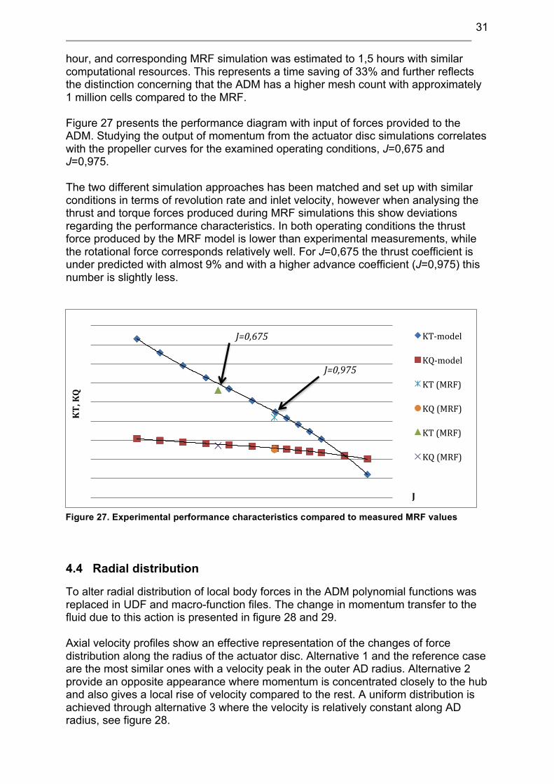
hour, and corresponding MRF simulation was estimated to 1,5 hours with similar computational resources. This represents a time saving of 33% and further reflects the distinction concerning that the ADM has a higher mesh count with approximately 1 million cells compared to the MRF. Figure 27 presents the performance diagram with input of forces provided to the ADM. Studying the output of momentum from the actuator disc simulations correlates with the propeller curves for the examined operating conditions, J=0,675 and J=0,975. The two different simulation approaches has been matched and set up with similar conditions in terms of revolution rate and inlet velocity, however when analysing the thrust and torque forces produced during MRF simulations this show deviations regarding the performance characteristics. In both operating conditions the thrust force produced by the MRF model is lower than experimental measurements, while the rotational force corresponds relatively well. For J=0,675 the thrust coefficient is under predicted with almost 9% and with a higher advance coefficient (J=0,975) this number is slightly less.

4.4 Radial distribution

To alter radial distribution of local body forces in the ADM polynomial functions was replaced in UDF and macro-function files. The change in momentum transfer to the fluid due to this action is presented in figure 28 and 29. Axial velocity profiles show an effective representation of the changes of force distribution along the radius of the actuator disc. Alternative 1 and the reference case are the most similar ones with a velocity peak in the outer AD radius. Alternative 2 provide an opposite appearance where momentum is concentrated closely to the hub and also gives a local rise of velocity compared to the rest. A uniform distribution is achieved through alternative 3 where the velocity is relatively constant along AD radius, see figure 28.

KT,  KQ  

J  

KT-­‐model  

KQ-­‐model  

KT  (MRF)  

KQ  (MRF)  

KT  (MRF)  

KQ  (MRF)  

J=0,675  

J=0,975  

Figure 27. Experimental performance characteristics compared to measured MRF values

32

Studying the tangential velocity component this demonstrate a similar behaviour, as seen in figure 29. The variations are however slightly bigger compared to the axial component and alternative 3 has an almost sinusoidal look along the radius, related to the shape of polynomial function inputted to the ADM.

Figure 28. Axial velocity component for radial distribution cases

Figure 29. Tangential velocity component for radial distribution cases

33

4.5 Non-uniform inflow

Through creation of a porous media zone the inflow field to the AD was affected, causing an inhomogeneous surface load onto the propeller disc. Simulation case ‘PM I’ can be seen in figure 30, with an overview of the axial velocity both in the flow direction and a cross-section normal to the flow, upstream of the AD. In the left part of the figure, stagnation can be seen due to deceleration of fluid reaching the porous zone. This also causes an increased velocity around this area. Calculation of average velocity in the CIA amounts to 2,65 m/s, leading to an operating condition of approximately J=0,65 (with the constant rotational speed 16,07 rps). Acceleration of water in the actuator disc is still uniform, however disturbed by the inflow conditions and particularly in the bottom region where fluid motion is low. The induced velocity field behind the AD becomes irregular with amplification in the top region and counteracted in lower regions because of an area of stagnation.

Simulation ‘PM II’ with change of porous media set up provided related flow scenarios as these shown in figure 30. With increased fluid resistances the velocity in CIA was calculated to 1,97 m/s, corresponding to a J=0,482, and nearly prevented any fluid through the bottom region. Remaining simulation ‘PM III’ resulted in CIA velocity of 3,31 m/s with J=0,808 and concerned higher permeability in all porous zones, which meant less disturbance of the flow field. The fluid slowdown in front of the porous domain also causes interaction with the inlet velocity boundary, according to pressure contours of the flow. This implies a need for extension of the fluid domain to prevent impact from outer boundaries. Placement of the CIA closer to the AD is also a fact that should be considered in terms of the suction effect due to acceleration of water.

Figure 30. Axial velocity profile in flow direction (left) and cross-section upstream of AD (right)

34

5 Discussion

Results from the initial mesh sensitivity analysis give an indication of the importance of discretization method and spatial resolving. The simulations conclude that a higher cell count, concentrated to the flow regions with large gradients of velocity and pressure, where analysis of data is conducted provides the most reliable solution. This corresponds with the information in an article from Morgut and Nobile (2012) where the authors further debate between potentials and drawbacks regarding a structured or unstructured mesh. A hybrid-unstructured mesh often compels less work when generating it, although showed the structured mesh a better behaviour concerning diffusivity and might therefore be regarded in continuing mesh studies. However does the ADM model seem to respond with some inconsistency when considering the mesh case nr 4, with reduced refinement zone yet still input of a low element size (5 mm). This specific set up yields a rather high cell count of 3 million elements and should impose on a reasonable level of resolving. The result during this simulation proved a significant disparity of induced velocity compared to the other mesh cases and was unexpected in relation to the lower resolution simulations. This questions the robustness of the model and numerical set up, though according to several of the articles and literature studied are effects related to discretization quite common. Since the case with highest mesh resolution was well aligned with the reference in both axial and tangential velocity components this was judged as acceptable for further studies. As a means of verifying the convergence process between the separate simulations each case were given additional iterations while monitoring the residual values. Doubling the amount of calculations showed no sign of sudden fluctuations and the induced velocity profiles remained intact, thus was convergence deemed as not influencing the result in an undesirable way. Studying the drag force along the shaft showed minor periodic oscillation, which is possibly the consequence of flow separation downstream. This may indicate effects relating to unsteady conditions where a stationary solution can be limiting, by preventing transient build-up of eddies in several directions. The dissymmetry of velocity components for the ADM, visible in figure 23 and 24, also implies for possible transient behaviour in the simulations. Comparing the actuator disc approach and MRF simulation resulted in some deviations of the induced velocity profile and its magnitude. The axial component showed good agreement of velocity profiles however was the AD induced velocity noticeably lower than the one from the actual propeller blade. In opposite were tangential velocities more even in terms of magnitude and less similar in the radial distribution. In an article of Gao et al. (2012) a similar behaviour is described, with under prediction of the axial component regarding a momentum source model. The reason for this might be related to geometrical differences where the actual propeller blade influence the flow pattern with the result of local increase of velocity and concentration of torque at a particular propeller radius. The two numerical methods are based on different solving techniques and certain error between the simulations was therefore expected. This fact, combined with that results from MRF simulations are entirely numerical in respect to these of the ADM, based on experimental model scale testing, suggests that the modelling approaches perform relatively well. The discrepancy is within levels achieved in the literature when considering open water characteristics, and the simulations during different

35

operating conditions demonstrate an adequate behaviour. The improvement in solving efficiency utilizing the ADM was at a first glance somewhat modest. A saving that totals one third of the time required concerning the MRF was less than expected, though should this number be regarded in the light of a 40% higher mesh count associated with ADM model. This greatly affects computational time and further reflects the differentiation between the numerical set up. A more equal resolving would likely generate additional advantages in efficiency with the actuator disc method and this might be achieved by implementing a different meshing approach or development of the geometrical domain. Though, with current ADM structure there is an opportunity of importing a rudder design into the geometry and enable direct interaction studies. Coupling in this manner provides a possibility of further propeller-rudder investigations; hence improving the applicability of the simulation model. Another promising aspect with the simplified ADM method can be described as the flexibility in studying multiple propeller designs. With limited effort in geometrical set up the ADZ dimensions can be altered, this together with updated propeller performance data allows simulations for several designs and propeller types. When examining the radial distribution of thrust and torque forces a difference between the ADM and MRF model was manifested concerning the tangential component. MRF simulations showed a velocity distribution concentrated closer to the shaft, which may suggest a separate torque distribution input for the ADM as to simulate this behaviour. The topic of radial distribution is discussed in articles from Philips et al. (2010) and Hough and Ordway (1965) in regard to different approaches for capturing effects onto the rudder. In the examined cases of force distribution in this thesis the ability to influence velocity profiles was clearly shown and therefore pose as a useful tool. The simulation with a prescribed root distribution, alternative 2, actually correspond relatively well with the MRF case in terms of the tangential component. Optimizing these input parameters with intention of attaining a representative flow scenario should thus be further looked into. Several of the articles referred to in this work argues for the meaning of used turbulence model. This is concluded as affecting both the numerically achieved simulation results and solution efficiency. This parameter need more examining, however is the SST k-ω described as a reliable model concerning the resolving of a near-wall boundary layer, capturing flow separation behaviour as well as being computationally efficient. As a means of being comparable both the ADM and MRF simulations has been performed using this specific solver. Concerning the simulation cases for the ADM being subjected to a non-uniform inflow velocity field initial results demonstrated a possible employment of a porous media. The flow field was influenced through the regions with varying permeability, which provided an ability to create an inhomogeneous surface load onto the propeller disc. This scenario represents the usual inflow inside a ship wake, to which a marine propeller is subjected to (Gaggero et al. 2010). To imitate this inflow behaviour is regarded vital for a more consistent analysis taking into account thrust and torque fluctuations, and the vibrations and noise this may lead to. The porous media zone caused a lowering of the fluid velocity, and was perceived in calculation of the average velocity in the CIA. This meant a change in operating

36

conditions with lower induced velocities as a consequence. However, due to the velocity averaging was the acceleration of water unaffected and still uniform in the actuator disc. Thus, as to represent the actual inhomogeneous inflow condition the CIA field require development into a sectorial partitioning similar to the one of the porous zone. This would enable an induced velocity dependent on the non-uniform inflow detected in the separate CIA regions and hopefully achieve a more realistic propeller flow case. Much work remain in determining the applicability of this method and the result also implies a need for change of geometrical domain for preventing interference due to surrounding boundaries. As been discussed earlier there is a lot more to be done in evaluating the performance of this momentum source simulation model. To summarize a few concerns for future work the list below is presented;

• Comprehensive focus on discretization methods as to minimize errors and improve solution efficiency

• Study including comparison of several propeller designs and operating conditions

• Further investigations of radial distribution and its potentials

• Comparison of the impact due to applied turbulence model

• Partitioning of CIA

37

6 Conclusions

The aim with this thesis has been to implement a fast simulation model for studies of the propeller-induced velocity field, and by extension effects regarding the interaction between propeller and rudder. Using a simplified approach with an actuator disc has demonstrated both promising initial results and some challenges where a lot of work is yet to be done. The ADM can be considered as still being in a prototype stage with possible further development in the future as to become an applicable and useful design tool. Principal conclusions from the simulations performed in this study are;

- Computational efficiency is improved with 33% compared to a more complex geometry case

- The modelling approach enables simple employment of different propeller types based on their specific propeller performance characteristics

- Induced velocity profiles correspond relatively well with the MRF simulations in

regard to their diverse numerical set up

- The mesh sensitivity analysis showed some unpredictable deviations, which compels thorough examining of discretization methods

- Possible development into non-uniform inflow conditions by employing a

porous media zone

38

7 List of References

Andersen, S.J., Lignarolo, L.E.M., Ragni, D., Ferreira, C.J.S., Sørensen, J.N., Mikkelsen, R.F. & Van Bussel, G.J.W. (2014). Comparison between PIV measurements and computations of the near-wake of an actuator disc. Journal of Physics: Conference Series, 524 (1).

ANSYS Theory Guide. (2015). Online resource. [Elektronisk]. Pennsylvania (USA): ANSYS Inc. Tillgänglig: http://www.ansys.com/Resource+Library [2015-02-22].

Benini, E. (2004). Significance of blade element theory in performance prediction of marine propellers. Ocean Engineering, 31 (8-9), 957-974.

Carlton, J. (2012). Marine Propellers and Propulsion. (2nd edn.). Burlington (USA): Butterworth-Heinemann.

Durante, D., Dubbioso, G. & Testa, C. (2013). Simplified hydrodynamic models for the analysis of marine propellers in a wake-field. Journal of Hydrodynamics, 25 (6), 954-965.

Gaggero, S., Villa, D. & Brizzolara, S. (2010). RANS and PANEL method for unsteady flow propeller analysis. Journal of Hydrodynamics, 22 (5 SUPPL. 1), 547-552.

Gao, Q., Jin, W. & Vassalos, D. (2012). The calculations of propeller induced velocity by RANS and momentum theory. Journal of Marine Science and Application, 11 (2), 164-168.

Greco, L., Muscari, R., Testa, C. & Di Mascio, A. (2014). Marine propellers performance and flow-field prediction by a free-wake panel method. Journal of Hydrodynamics, 26 (5), 780-795.

Hough, G.R. & Ordway, D.E. (1965). The generalized actuator disc. Developments in Theoretical and Applied Mechanics, 2 , 317-336.

Keon-Je Oh & Shin-Hyoung Kang (1995). Numerical calculation of the viscous flow around a propeller shaft configuration. International Journal for Numerical Methods in Fluids, 21 (1), 1-13.

Kerwin, J. (2001). Hydrofoils and propellers. Cambridge: MIT. Tillgänglig: http://ocw.mit.edu/courses/mechanical-engineering/2-23-hydrofoils-and-propellers-spring-2007/course-notes/kerwin_notes.pdf [2015-03-10].

Menter, F.R. (1994). Two-equation eddy-viscosity turbulence models for engineering applications. AIAA Journal, 32 (8), 1598-1605.

Morgut, M. & Nobile, E. (2012). Influence of grid type and turbulence model on the numerical prediction of the flow around marine propellers working in uniform inflow. Ocean Engineering, 42 , 26-34.

39

Munson, B., Okiishi, T., Huebsch, W. & Rothmayer, A. (2013). Fluid Mechanics. (7th edn.). Hoboken, NJ (USA): Wiley.

Phillips, A.B., Turnock, S.R. & Furlong, M. (2010). Accurate capture of propeller-rudder interaction using a coupled blade element momentum-RANS approach. Ship Technology Research, 57 (2), 128-139.

Rhee, S.H. & Joshi, S. (2006). Computational validation for flow around a marine propeller using unstructured mesh based Navier-Stokes solver. JSME International Journal, Series B: Fluids and Thermal Engineering, 48 (3), 562-570.

Rolls-Royce. (2015). Computer Aided Engineering (CAE) Team. Hydrodynamic Research Centre (Kristinehamn).

Sánchez-Caja, A., Martio, J., Saisto, I. & Siikonen, T. (2014). On the enhancement of coupling potential flow models to RANS solvers for the prediction of propeller effective wakes. Journal of Marine Science and Technology, 20 (1), 104-117.

Tornblad, J. (1990) Marine propellers and propulsion of ships. Kristinehamn: KaMeWa Marine laboratory.

Tritton, D.J. (1977). Physical Fluid Dynamics. (1st edn.). Berkshire (UK): Van Nostrand Reinhold.

Versteeg, H. & Malalasekera, W. (2007). An Introduction to Computational Fluid Dynamics: The Finite Volume Method. (2nd edn.). Essex (UK):Pearson.

Vyšohlíd, M. & Mahesh, K. (2007). Understanding crashback in marine propellers using an unsteady actuator disk model. In Collection of Technical Papers - 45th AIAA Aerospace Sciences Meeting. 11133.

Wikimedia commons. (2000). Basic three dimensional cell shapes (Shyam2791). [Elektronisk]. Tillgänglig: http://upload.wikimedia.org/wikipedia/commons/d/dc/Three_Dim_Grid.PNG [2015-06-08].

Windén, B., Turnock, S. & Hudson, D. (2014). A RANS modelling approach for predicting powering performance of ships in waves. International Journal of Naval Architecture and Ocean Engineering, 6 (2), 418-430.