UTILIZING DISTRIBUTED TEMPERATURE AND PRESSURE DATA TO

EVALUATE THE PRODUCTION DISTRIBUTION IN MULTILATERAL

WELLS

A Thesis

by

RASHAD MADEES K. AL ZAHRANI

Submitted to the Office of Graduate Studies of Texas A&M University

in partial fulfillment of the requirements for the degree of

MASTER OF SCIENCE

May 2011

Major Subject: Petroleum Engineering

Utilizing Distributed Temperature and Pressure Data to Evaluate The Production

Distribution in Multilateral Wells

Copyright 2011 Rashad Madees K. Al-Zahrani

UTILIZING DISTRIBUTED TEMPERATURE AND PRESSURE DATA TO

EVALUATE THE PRODUCTION DISTRIBUTION IN MULTILATERAL

WELLS

A Thesis

by

RASHAD MADEES K. AL ZAHRANI

Submitted to the Office of Graduate Studies of Texas A&M University

in partial fulfillment of the requirements for the degree of

MASTER OF SCIENCE

Approved by:

Chair of Committee, Ding Zhu

Committee Members, Daniel Hill Wolfgang Bangerth

Head of Department, Steven Holditch

May 2011

Major Subject: Petroleum Engineering

iii

ABSTRACT

Utilizing Distributed Temperature and Pressure Data To Evaluate The Production

Distribution in Multilateral Wells. (May 2011)

Rashad Madees K. Al-Zahrani, B.S., Texas A&M University

Chair of Advisory Committee: Dr. Ding Zhu

One of the issues with multilateral wells is determining the contribution of each

lateral to the total production that is measured at the surface. Also, if water is detected at

the surface or if the multilateral well performance declines, then it is difficult to identify

which lateral or laterals are causing the production decline.

One way to estimate the contribution from each lateral is to run production

Logging Tools (PLT). Unfortunately, PLT jobs are expensive, time-consuming, labor-

intensive and involve operational risks. An alternative way to measure the production

from each lateral is to use Distributed Temperature Sensing (DTS) technology. Recent

advances in DTS technology enable measuring the temperature profile in horizontal

wells with high precision and resolution. The changes in the temperature profile are

successfully used to calculate the production profile in horizontal wells.

In this research, we develop a computer program that uses a multilateral well

model to calculate the pressure and temperature profile in the motherbore. The results

iv

help understand the temperature and pressure behaviors in multilateral wells that are

crucial in designing and optimizing DTS installations. Also, this model can be coupled

with an inversion model that can use the measured temperature and pressure profile to

calculate the production from each lateral.

Our model shows that changing the permeability or the water cut produced from

one lateral results in a clear signature in the motherbore temperature profile that can be

measured with DTS technology. However, varying the length of one of the lateral did not

seem to impact the temperature profile in the motherbore. For future work, this research

recommends developing a numerical reservoir model that would enable studying the

effect of lateral inference and reservoir heterogeneity. Also recommended is developing

an inversion model that can be used to validate our model using field data.

v

DEDICATION

To a casual observer, this thesis might appear to be a solitary work. However, to

complete such a journey requires a great deal of support, encouragement and discipline,

and I am indebted to my father and mother for supporting me all the way. There is

nothing in the world I can do to pay them back but I know my academic and professional

success gives them the greatest satisfaction.

I am also so grateful to my beautiful wife, Haifa, who completed her M.S. in

economics this semester. Despite being so busy, she still managed to be the lovely and

supportive wife I have always known. Also, I am so thankful to my brother and sister for

their prayers and support. Last but not least, I always thank God, Allah, for blessing me

with my cute, funny and energetic daughter, Lamar.

vi

ACKNOWLEDGEMENTS

I am heartily thankful to my advisor, Dr. Ding Zhu, for her support and guidance

throughout this research, and for her trust in my abilities and interests. My special thanks

to her for being so patient in teaching me such an involved topic that transformed my

understanding of Distributed Temperature Sensing (DTS) technology and its application

in wellbore flow modeling.

I am also so grateful to Dr. A. Daniel Hill and Dr. Wolfgang Bangerth for their

willingness to serve as members on this thesis committee and for being always available

to help and comment on my work as needed.

Finally, many thanks to the great Saudi community in College Station, TX for

making our stay here so enjoyable. Among my Saudi colleagues, I would like to thank

Jassim Al-Mullah, Bandar Al-Khamis, Abduallah Al-Yami, and Abdullwahab Al-

Ghamdi, for being so nice and supportive during my stay here in the United States.

vii

NOMENCLATURE

Symbol Description

Specific density

µ Viscosity

C Casing

cem Cement

Cp Specific heat capacity

CV

Parameter used in the calculation of pressure drop across ICV’s that accounts for how the pressure changes with the

changing the opening of the valve

D Diameter

D* Dimensionless diameter

DTS Distributed temperature sensing

F Friction factor

f0 Friction factor without inflow effect

G Acceleration of gravity, 9.8 m/s

G Gas

H Enthalpy

I A certain phase

Iani Anistropy ratio

ICV Inflow Control Valve

In Inflow

J A certain segment

viii

Symbol Description

K Permeability

kH Horizontal permeability

KJT Joule-Thompson coefficient

KT Formation conductivity

Ku Kutateladze number

kV Vertical permeability

L Length

L Liquid

ML Multilateral

N Maximum number of segments in the wellbore

NRe Reynolds number in pipe

NRe,w The inflow Reynolds number

O Oil

P Pressure

Pr Prandtl number

Q Flow rate

Q Heat Flux

R Indicates the radial direction

rw Wellbore radius

T Temperature

Tp Two-phase

ix

Symbol Description

U Overall heat transfer coefficient in a pipe; not perforated

Uoverall Overall heat transfer coefficient including inflow effect

V Velocity

W Water

X Liquid fraction

X Indicates the direction along the pipe

y Fraction of a phase in a fluid

yb Half the width of the box-shaped reservoir in Furui’s model

Α Gas fraction

Λ Fraction of segment that is open area

Ρ Density

Σ Surface tension

Τ Stress tensor

Φ Combined stress tensor

Ө Inclination angle

x

TABLE OF CONTENTS

Page

ABSTRACT .................................................................................................................... iii

DEDICATION ................................................................................................................ v

ACKNOWLEDGEMENTS ............................................................................................ vi

NOMENCLATURE ........................................................................................................ vii

TABLE OF CONTENTS ................................................................................................ x

LIST OF FIGURES ......................................................................................................... xii

LIST OF TABLES .......................................................................................................... xiv

1. INTRODUCTION ..................................................................................................... 1

1.1. Background ........................................................................................................ 1 1.2. Literature Review ............................................................................................... 4 1.3. Research Objectives ........................................................................................... 7 1.4. Organization of the Thesis ................................................................................. 9

2. WELLBORE MODEL .............................................................................................. 11

2.1. Introduction ........................................................................................................ 11 2.2. Mass Balance ..................................................................................................... 14

2.2.1. Single Phase Flow ..................................................................................... 14 2.2.2. Multiphase Flow ....................................................................................... 15

2.3. Momentum Balance ........................................................................................... 16 2.3.1. Single Phase Flow ..................................................................................... 16 2.3.2. Multiphase Flow ....................................................................................... 20

2.4. Energy Balance .................................................................................................. 25

xi

Page

2.4.1. Single Phase Flow ..................................................................................... 26 2.4.2. Multiphase Flow ....................................................................................... 34

3. RESERVOIR MODEL ............................................................................................. 36

3.1. Introduction ........................................................................................................ 36 3.2. Reservoir Pressure Model .................................................................................. 36 3.3. Reservoir Temperature Model ........................................................................... 38

4. COUPLED WELLBORE AND RESERVOIR MODEL .......................................... 42

4.1. Introduction ........................................................................................................ 42 4.1.1. Multilateral Well Model Assumptions ..................................................... 42

4.2. Coupled Pressure Model .................................................................................... 45 4.3. Coupled Temperature Model ............................................................................. 52

4.3.1. Temperature Calculation in each Lateral .................................................. 52 4.3.2. Temperature Calculation in the Motherbore ............................................. 55

5. RESULTS AND DISCUSSION ............................................................................... 59

5.1. Results for Horizontal Wells .............................................................................. 59 5.2. Results for Multilateral Wells ............................................................................ 68

6. CONCLUSIONS AND RECOMMENDATIONS .................................................... 87

6.1. Conclusions ........................................................................................................ 87 6.2. Recommendations .............................................................................................. 88

REFERENCES ................................................................................................................ 89

VITA .............................................................................................................................. 92

xii

LIST OF FIGURES

Page

Figure 1.1: Relative Development Unit Well Costs for HRDH Inc-3; Costs are Relative to Vertical Wells in $/BPD .............................................................. 2

Figure 1.2: A Typical Multilateral Well Drilled in Saudi Arabia; This is a Trilateral

Wells ................................................................................................................ 8 Figure 1.3: Top-View of a Trilateral Well Showing the Tubing, Packers and ICV

Installations .................................................................................................... 8 Figure 2.1: A Diagram showing the Lateral’s Segmentation Scheme and the Frame

of Reference ................................................................................................... 13 Figure 2.2: A Cross-Sectional Area of a Pipe Showing the Various Pipe, Cement,

and Casing Radii and the Locations of Pipe Temperature and Inflow Temperature .................................................................................................... 28

Figure 2.3: Segment Diagram Showing the Variables in Eq. (2.93) ................................. 34 Figure 3.1: Reservoir Model Showing the Well at the Center .......................................... 37 Figure 3.2: An End View Showing the Reservoir and the Wellbore at the Middle .......... 37 Figure 4.1: A Diagram of Three Laterals Connected to a Motherbore that Shows

the Segmentations, the Locations of the Valves and Packers ........................ 43 Figure 4.2: Pressure Calculation Process in Each Lateral ................................................. 47 Figure 4.3: Pressure Calculation Process in the Motherbore ............................................ 51 Figure 4.4: Wellbore Temperature Calculation Procedure in Each Lateral ...................... 54 Figure 4.5: Diagram Showing the Calculation Variables for the First Segment in

the Motherbore ............................................................................................... 56 Figure 4.6: Diagram Showing the Variables in a Junction Segment................................. 58 Figure 5.1: Pressure Profile for a Horizontal Well; 6” in Diameter .................................. 61 Figure 5.2: Temperature Profile for a Horizontal Well; 6” in Diameter ........................... 62

xiii

Page Figure 5.3: Pressure Profile for a Horizontal Well; 4” in Diameter .................................. 64 Figure 5.4: Temperature Profile for a Horizontal Well; 4” in Diameter ........................... 65 Figure 5.5: Pressure Profiles in the Wellbore for Oil and Water Cases, 4” Diameter ...... 67 Figure 5.6: Temperature Profiles in the Wellbore for Oil and Water Cases, 4”

Diameter ....................................................................................................... 67 Figure 5.7: Pressure Profile in the Motherbore; Base Case .............................................. 71 Figure 5.8: Temperature Profile in the Motherbore; Base Case ....................................... 71 Figure 5.9: Pressure Profiles for Cases where Permeability of L2 was Reduced ............. 75 Figurea5.10: Temperature Profiles for Cases where Permeability of L2 was

Reduced ...................................................................................................... 76 Figure 5.11: Pressure Profiles in the Motherbore; Cases where the Length was

Varied.......................................................................................................... 79 Figure 5.12: Temperature Profiles in the Motherbore; Cases where the Length was

Varied ........................................................................................................... 80

Figure 5.13: Pressure Profiles in the Motherbore; Cases where the Water Cut was Varied.......................................................................................................... 85

Figure 5.14: Temperature Profiles in the Motherbore; Cases where the Water Cut

was Varied .................................................................................................... 86

xiv

LIST OF TABLES

Page

Table 2.1: Kutateladze Numbers as a Function of Dimensionless Diameter, D* .......... 23

Table 4.1: The Values of CV Coefficients for a Smart Completion Valve, Valve Size is 3 1/2” ...................................................................................... 49

Table 5.1: Reservoir and Wellbore Data Summary for the Horizontal Well Case ........ 59

Table 5.2: Fluid Properties Used for Oil ........................................................................ 60

Table 5.3: Main Results from Horizontal Well Simulation ........................................... 60

Table 5.4: Fluid Properties Used for Water ................................................................... 66

Table 5.5: Summary of Oil and Water Runs at Different Drawdown Pressures ........... 66

Table 5.6: Key Parameter for the Motherbore, Base Case ............................................. 68

Table 5.7: Results for the Base Case for Motherbore .................................................... 70

Table 5.8: Description of the Simulation Runs .............................................................. 73

Table 5.9: Key Results for Simulation Runs where Permeability is Varied .................. 75

Table 5.10: Key Results for Simulation Runs where Length is Varied ......................... 78

Table 5.11: Inflow Temperatures for L2 for Runs#2-8 .................................................. 78

Table 5.12: Key Results for Simulation Runs where Water Cut is Varied .................... 82

Table 5.13: Key Results for Simulation Runs where Permeability is Varied, 4” Diameter ................................................................................................. 83

Table 5.14: Key Results for Simulation Runs where Length is Varied, 4” Diameter ................................................................................................. 84

Table 5.15: Key Results for Simulation Runs where Water Cut is Varied, 4” Diameter ................................................................................................ 84

1

1. INTRODUCTION

1.1 Background

Advances in drilling and completion technologies have enabled drilling more

complex well structures to increase productivity in a cost-effective manner. Horizontal

wells have been utilized to increase the reservoir contact area and thus increasing the

total production rate and improving the reservoir sweep efficiency. Also, horizontal

wells can be used to delay water encroachment by drilling at the top of productive

formations so to stay as far as possible from the water table. In addition, multilateral

wells have enabled accessing multiple formations from the same well while reducing

drilling foot print. One of the milestones in the application of multilateral well

technology, as Al-Kaabi (2008) indicated, is what Saudi Aramco have accomplished in

developing Haradh Inc-3, a subfield of the Ghawar field. The field was developed with

thirty two multilateral wells, predominantly trilateral wells, to achieve a target rate of

300 MBPD. This development scheme coupled with the inflow control valves (ICV’s)

enabled reducing the number of wells required for the target production rate as well as

the development cost per barrel as shown in Fig. 1.1, by Al-Kaabi (2008).

____________ This thesis follows the style of SPE Production & Operations.

2

Fig. 1.1: Relative Development Unit Well Costs for HRDH Inc-3; Costs are Relative to Vertical Wells in $/BPD.

Although they were intended as means of allocating hydrocarbons, temperature

logs were applied to analyze well production or injection profiles. Hill (1990) implied

that the applications focused on vertical wells, were more qualitative in nature and were

aimed at identifying anomalous behaviors in temperature profiles. These applications

included identifying gas entry zones, casing leaks and lost circulation zones. However,

in horizontal or near horizontal wells, Yoshioka (2007) indicated that the geothermal

gradient does not play an important role and that the temperature variation along the

wellbore is caused by subtle effects mainly; the fluid expansion and the viscous

dissipation effects. This small temperature change can be used to interpret openhole flow

profile.

Another challenge for horizontal wells is that the temperature variation is

estimated to be in the order of several degrees as reported by Yoshioka (2007) and

Dawkrajai (2006). Such difference cannot be detected with the conventional temperature

sensors run in ordinary temperature logs. However, Fiber-optic distributed temperature

sensing (DTS) technology enables detecting temperature changes in the order of 0.01oC

1.0

0.7

0.35

VERTICAL HORIZONTAL MRC/SMART

Re

lati

ve

Un

it C

os

t (D

ime

ns

ion

les

s)

3

with continuous monitoring ability for up to 60 km and with a short updating time of 10

seconds (Sensornet 2009). Also, DTS technology provides many advantages in

monitoring and optimizing well performance and integrity. The DTS is provided

continuously, real-time and requires no wellbore intervention. This provides cost-

effective and safe alternative to the conventional PLT jobs. Moreover, DTS technology

includes surface readout units that can be easily integrated into an existing network of

transferring and storing data which can be integrated in future development of intelligent

fields.

The increasing field installations of DTS technology show the increasing

confidence in the technology as well as the versatile applications. Nath et al. (2006) cited

successful application of DTS technology in Indonesia. The operator was able to monitor

the water breakthrough in a horizontal well and determine the pump- and motor-

operating conditions of the installed Electrical Submersible Pump (ESP). Also, this

information enabled the optimization of ESP installations in the area. Glasbergen et al.

(2009) presented a field case for a method to quantify the diversion effect for acid jobs.

They used a tracer slug concept and interpreted the temperature profile before and after

the treatment to infer the effectiveness of the diversion.

In Saudi Arabia, Hembling et al. (2010) reported several field applications of a

DTS system installed on a Multilateral well. The well was equipped with ICV’s to

control each lateral individually. The applications included the confirmation of ICV

operations and confirmation that the subsurface sliding door, SSD, has closed. Also and

4

more importantly, the effect of inflow from each lateral was seen on the temperature log

as spikes of increased temperature.

1.2 Literature Review

Hill (1990) implied that most of the earlier work using temperature logging was

on vertical wells with the focus on anomalies in the temperature profile because of gas

entry or on monitoring well integrity to identify casing leaks or lost circulation zones.

Also, the applications tended to be more qualitative in nature, identifying the place of the

anomaly, and less quantitative; i.e. determining the actual rates.

Dawkrajai (2006) studied the feasibility of using DTS data to infer production

profile and developed several synthetic cases to understand the range for temperature

changes caused by flow rates. He developed a numerical reservoir temperature and

pressure models coupled with multiphase wellbore flow model and solve the model

iteratively. He concluded that the two main contributors to the temperature profile in the

case of horizontal wells are the fluid thermal expansion and the viscous dissipation. He

also concluded that the wellbore temperature derivate showed a remarkable change when

different phase enters the wellbore especially for gas inflow zones. He showed that oil

and water enters the wellbore 3-4 oF higher than the geothermal but gas enters the

wellbore at 5-6 oF lower than the geothermal temperature. However, Dawkrajai indicated

that no –inflow zones were difficult to identify using DTS temperature data.

Yoshioka’s work (2007) paralleled that of Dawkrajai with the difference being in

the reservoir model. Yoshioka used the reservoir pressure model developed by Furui et

5

al. (2003). Furui assumed steady-state, box-shaped reservoir with the well fully

penetrating the entire reservoir and flow perpendicular to the wellbore and with no flow

in the axial direction. He divided the reservoir into two regions according to the

streamline shape; the linear region from the boundaries to a certain distance from the

wellbore and a radial region extending from the wellbore wall to a certain distance into

the reservoir. Combining the solutions in both regions, He solved for the total rate and

showed a good agreement with reservoir simulation results. Following the same

approach, Yoshioka assumed steady-state conditions and developed analytical reservoir

temperature models for the linear and radial regions. He then combined both solutions to

come up with final solution for the temperature profile in the reservoir. From the

reservoir model, Yoshioka concluded that the temperature profile increased gradually in

the linear region and rapidly in the radial region. Also, he was able to simplify the

reservoir temperature solution by ignoring the heat conduction term in the linear region

without compromising on the accuracy of the solution. Additionally, Yoshioka

developed an inversion model and presented its applicability using production log data

on a horizontal well in the North Sea in which he was able to match the pressure and

temperature profiles and successfully estimate the inflow rates.

Sui (2009) detailed a method of using DTS transient temperature and pressure

data to characterize properties of multilayered reservoirs in vertical wells. Her findings

showed that the temperature data can be used to determine the radius of damage which

cannot be determined from the pressure data alone.

6

Hembling et al. (2008) presented a field installation of a DTS system in a

multilateral well. The temperature profile measured enabled Saudi Aramco to confirm

that the downhole inflow control valves (ICV) are operating and to monitoring the

displacement of diesel in the annulus through the Selective Shutting Device (SSD). After

six weeks, the well was put on production and the temperature profile clearly showed the

inflow at the laterals since the fluid from the laterals entered the motherbore at a higher

temperature than the fluid in the motherbore.

To develop models to account for small temperature and pressure changes, a

detailed wellbore model has to be developed. Numerous wellbore multiphase flow

models are present in the petroleum engineering literature, Shoham (2006), including the

drift-flux and mechanistic modeling. The drift-flux model is easier to implement in

simulation work and is the one commonly used in commercial reservoir simulators. Shi

et al. (2005) conducted extensive experimental work to determine the appropriate values

for the drift-flux model parameters for water/gas, oil/water and oil/water/gas systems.

Their calculated parameter values show excellent agreement with the experimental data.

Ouyang (1998) developed a homogeneous model to calculate the pressure drop in

horizontal wells for the gas/liquid system. The liquid phase treated oil and water as a

homogeneous phase using mixture properties that are weighted based on volumetric

ratios. Their model accounts for the inflow effect and shows a good agreement with the

experimental data.

7

1.3 Research Objectives

The objective of this research is to develop a theoretical model and a computer

program that performs forward calculation of the temperature and pressure profiles in

multilateral wells. Given the reservoir conditions and well configuration, the model will

generate a pressure and temperature profile in the motherobore which is the main bore

connecting with the laterals. The results will help understand the temperature and

pressure behavior in multilateral wells which is crucial in designing and optimizing

future DTS installations. Moreover, this program can be coupled with an inversion

model in which the production from each lateral is calculated based on the measured

temperature and pressure profiles. This will have great utility to field-operating

companies when performing production testing jobs as the contribution from each lateral

can be determined real-time. Since the DTS system is permanently installed, continuous

production profile will be generated that will help in future optimizations and enable

detecting water or gas breakthrough.

To better understand the problem and the assumptions made in developing this

model, a brief description of the system installation is needed. This study will use

specific multilateral well configurations. We will use trilateral or dual wells normally

drilled in the same formation and at almost the same elevation. Sometimes, a small

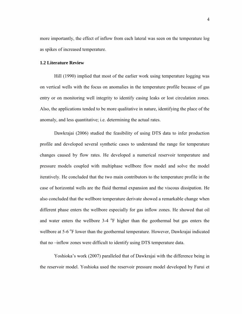
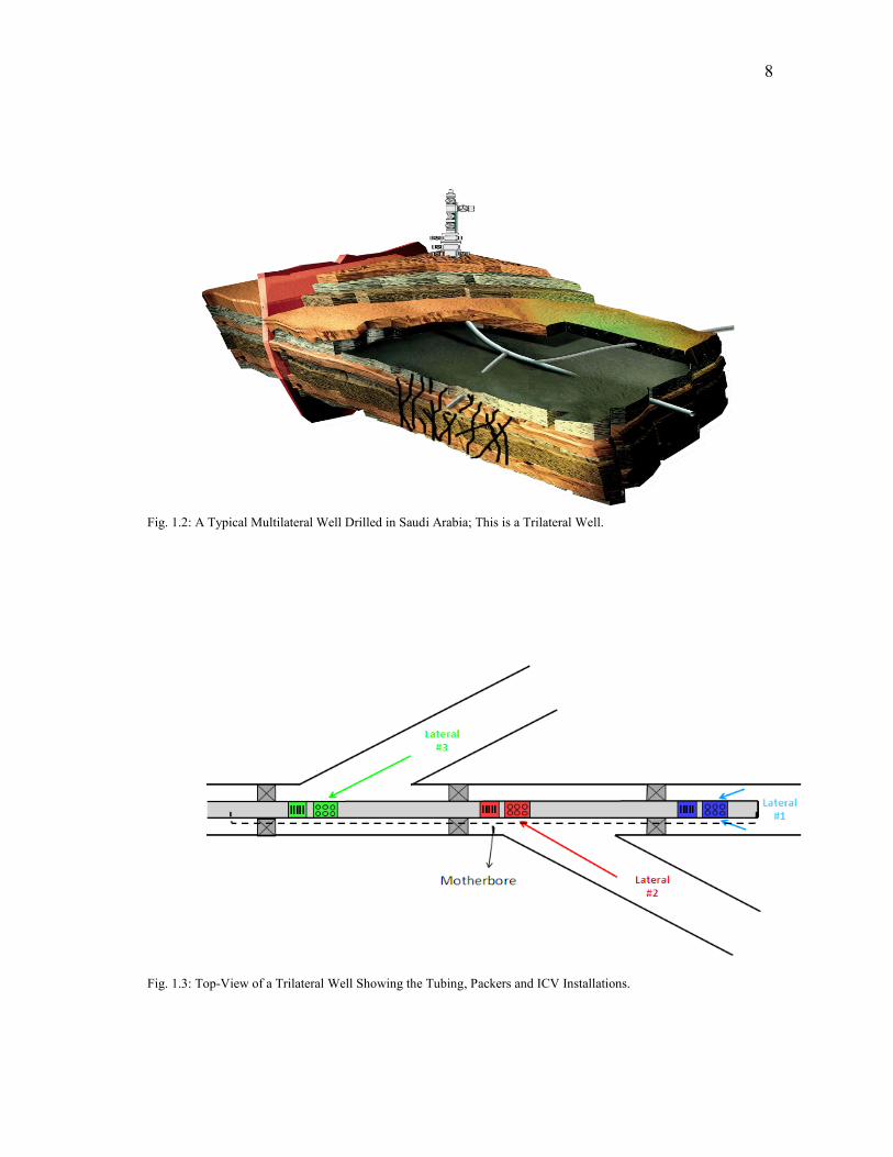
inclination exists. Fig. 1.2 and Fig. 1.3 show diagrams of a typical installation. The

production tubing is run in the motherbore and is bullnosed; tubing is closed at the end.

Therefore, all the flow comes through the ICV and production from all laterals is

comingled in the motherbore.

8

Fig. 1.2: A Typical Multilateral Well Drilled in Saudi Arabia; This is a Trilateral Well.

Fig. 1.3: Top-View of a Trilateral Well Showing the Tubing, Packers and ICV Installations.

9

The DTS and pressure sensors are installed in the interior of the motherbore pipe.

The fiber-optic cables are clapped on the tubing and run from the toe of the well, total

depth, all the way to the wellhead. The data is transferred and stored in a surface readout

unit where it can be retrieved for further analysis. This feature makes DTS technology

more compatible with intelligent field applications where monitoring and control is

envisioned to be performed real-time and remotely with minimum field personnel

involvement on the wellsite.

1.4 Organization of the Thesis

The second Section of this thesis will discuss the development of the wellbore

model. Section 2.1 will describe the geometry of the model considered and the

assumptions made. Attempts will be made to explain the validity and the value of each

assumption. In Section 2.2, we will derive the mass balance equations for the single and

multiphase flow conditions. Section 2.3 will present the derivation of the momentum

balance equations for single and multiphase flow conditions which determine the

pressure drop in the wellbore. In Section 2.4, we derive the energy balance equation for

the single and multiphase flows which describe the temperature profile in the wellbore.

All the equations will be written in a discrete form using finite difference approximation

as this will be the form used in the actual model. Section 3 will discuss the reservoir

model; both the pressure and temperature models along with the important assumptions

made. The details of the derivation will not be shown as the model has been derived

several times before by Furui (2003), Dawkrajai (2006) and Yoshioka (2007) and we use

the exact same formulation. After that, Section 4 will present the coupling of wellbore

10

and reservoir models to generate the pressure and temperature profiles. In this Section,

we will detail all the steps and assumptions made in our model. In Section 5, we will

start by examining results for horizontal wells. These results will help us analyze and

interpret our results for multilateral wells. After that, we will study the effect of varying

several parameters like permeability, wellbore length and water cut on temperature

profiles in multilateral wells. Finally, Section 6 will present the research conclusions and

recommendations.

11

2. WELLBORE MODEL

2.1 Introduction

Multilateral wells consistent of two or more horizontal laterals that are tied to a

main bore, the motherbore, in which the production is comingled, as shown by Fig 1.2.

Therefore, the first step in developing a multilateral well model is to derive the equations

used for each of the horizontal laterals. In this Section, we derive the wellbore model.

Our approach is to develop the mass balance, momentum balance and energy balance in

discrete forms using finite-difference method. Because of the different flow phenomena

between single and multiphase flows, two sets of equations will be developed for each

case; i.e. for the single phase and multiphase flow cases. The finite difference forms will

be used for the coupled model presented in Section 4. The wellbore model derivation

parallels Yoshioka’s (2007) derivation but with some modifications on the notations,

assumptions and correlations used.

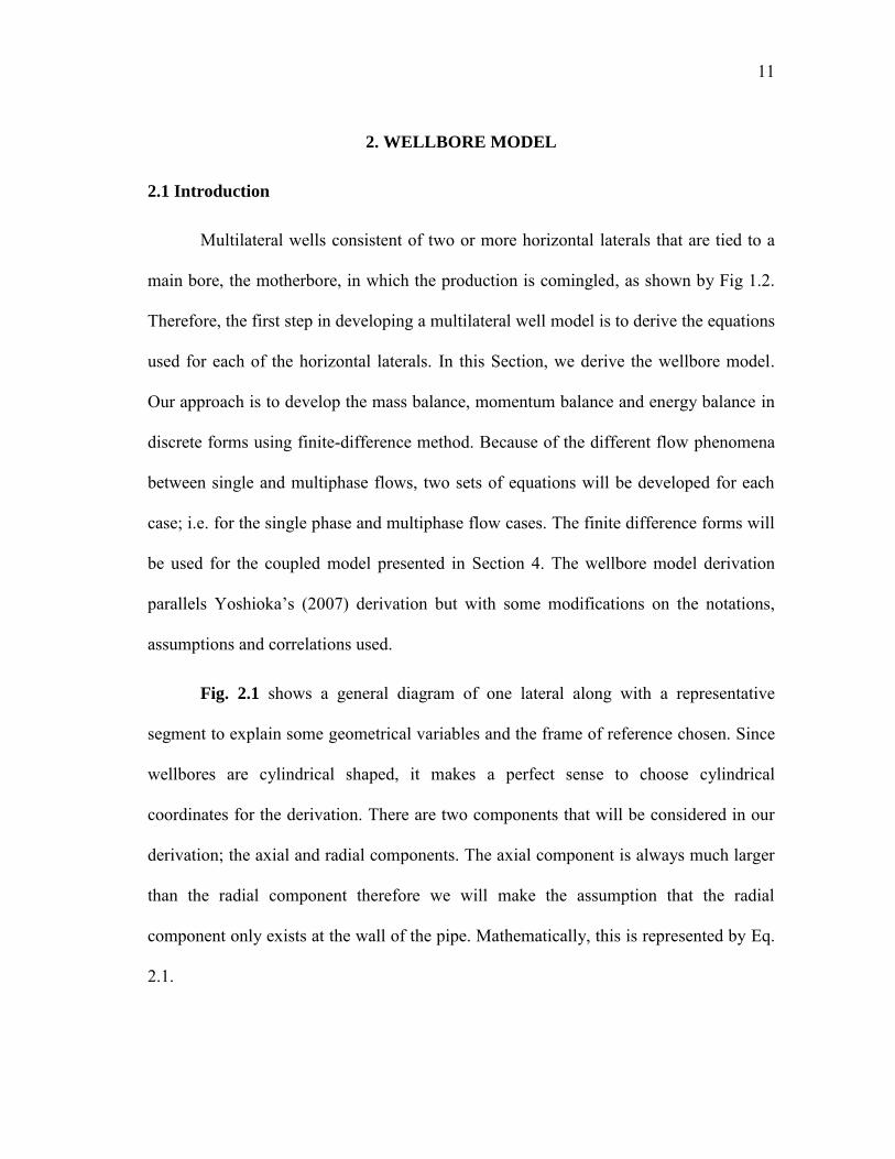
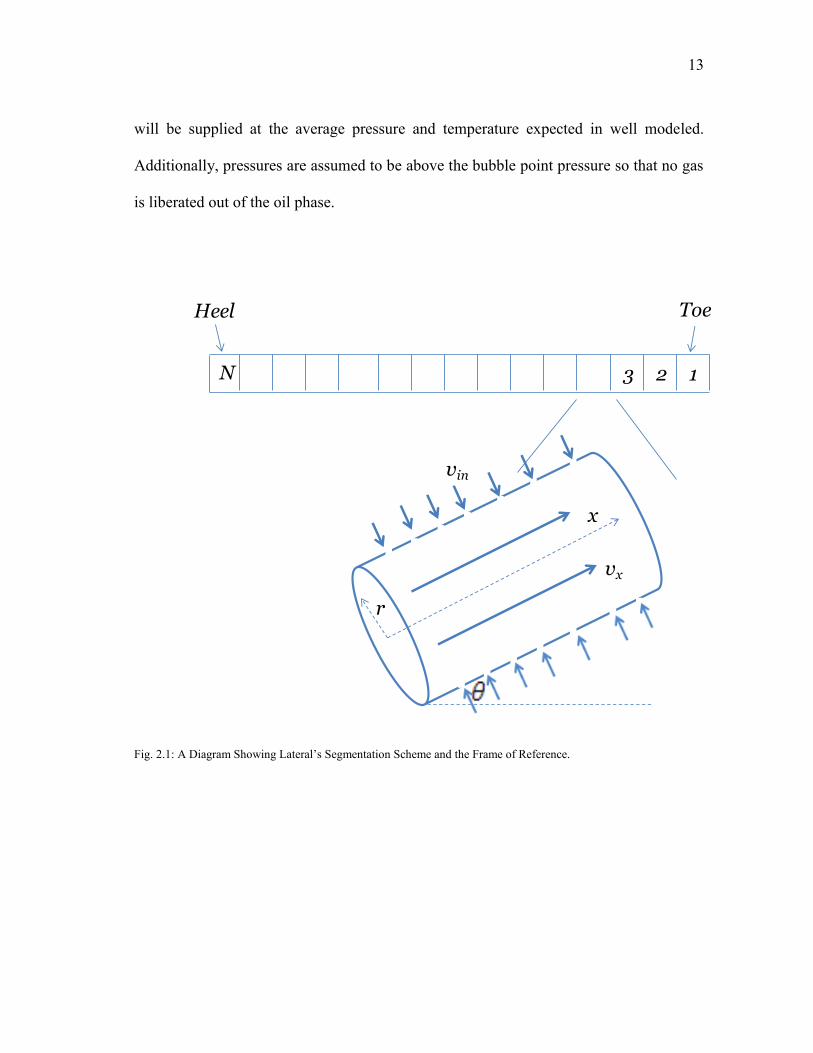
Fig. 2.1 shows a general diagram of one lateral along with a representative

segment to explain some geometrical variables and the frame of reference chosen. Since

wellbores are cylindrical shaped, it makes a perfect sense to choose cylindrical

coordinates for the derivation. There are two components that will be considered in our

derivation; the axial and radial components. The axial component is always much larger

than the radial component therefore we will make the assumption that the radial

component only exists at the wall of the pipe. Mathematically, this is represented by Eq.

2.1.

12

The radial distance “rw” represents the wellbore radius. Also, wellbores can have

different types of completions ranging from openhole to casing and perforated. Fig. 2.1

shows case of a perforated segment and to account for the fact that part of the segment

can be closed and not open for flow, we introduce the variable (λ) defined as follows;

The value of this parameter is one for openhole completion and is equivalent to

the perforation density for a perforated segment. The inflow velocity ( is calculated

by Eq. 2.3 using the inflow rate which is determined by Furui’s equation which will be

explained in Section 3.

where “j” represents a certain segment.

Throughout our derivation for the wellbore model, we will assume that the well

has been flowing for a period of time long enough to achieve a steady-state conditions.

Moreover, in the problem we are investigating, the pressure and temperature variations

are not significant since all the laterals in a ML well are drilled in the same formation at

almost the same elevations. Therefore fluid properties are assumed to be constants and

13

will be supplied at the average pressure and temperature expected in well modeled.

Additionally, pressures are assumed to be above the bubble point pressure so that no gas

is liberated out of the oil phase.

Fig. 2.1: A Diagram Showing Lateral’s Segmentation Scheme and the Frame of Reference.

123N

Heel Toe

x

r

vin

vx

14

2.2 Mass Balance

2.2.1 Single Phase Flow

In steady-state conditions, conservation of mass states that the rate of mass

entering the system must equal to the rate of mass exiting. Mathematically this

relationship is represented by Eq. 2.4, Eq. 2.5 and Eq. 2.6.

Substituting Eq. 2.5 and Eq. 2.6 into Eq. 2.4 and cancelling out the density since

it is assumed to be constant gives

Rearranging Eq. 2.7 and dividing by gives

Assuming that the wellbore is divided into segments and using the subscript, j, to

refer to a specific segment, Eq. 2.8 can be written in its final form as shown below.

15

2.2.2 Multiphase Flow

For multiphase flow, we will use the subscript “i” to indicate a certain phase and

the subscript “j” to indicate a certain segment. We apply Eq. 2.5 and Eq. 2.6 for each

phase as follows

Rate of mass input should equal to the rate of mass output, therefore we set Eq.

(2.10) and Eq. (2.11) equal, we obtain Eq. (2.12)

We rearrange and divide by ( to obtain Eq. (2.13)

As we indicated earlier, we assume the fluid properties are constant; therefore we

cancel out the density. Also, we arrange Eq. (2.13) to obtain the differential form and

take the limit of as follows

where “ is the volume fraction of phase “i”.

16

It is worth noting that we do not include the volumetric fraction in the inflow

term since we assume single phase flow in the reservoir for each segment; Section Three

explains the reservoir model in details.

Now, we use the finite difference approximation to obtain the discrete form of

Eq. (2.14)

2.3 Momentum Balance

The aim of the momentum balance is to obtain equations to solve for the pressure

drop in the pipe. As we did with the mass balance, we will first derive the equations for

the single phase case then for the multiphase flow case.

2.3.1 Single Phase Flow

Eq. 2.16 represents the momentum balance mathematically;

We use the combined rate of momentum flux equation defined by Bird et al.

(2002) which is shown by Eq. 2.17.

17

The first term is the convective rate of momentum-flux tensor and the last two

terms represent the molecular rate of momentum flux tensors. That is, all the terms have

dimensions of momentum per unit time per unit area.

In our problem, we are only concerned about two components of the combined

rate of momentum flux which can be expanded as follows

and

Furthermore, the component of the shear stress caused by flow along the x-

direction and perpendicular to it can be expanded using Newton’s law of viscosity and

ignoring the dilatational viscosity as follows;

For the third term in Eq. 2.16, we only consider force by gravity which

represented by Eq. 2.21

However, we will only consider horizontal or near horizontal wellbores so this

gravity term will be neglected. Based on our geometry represented by Fig. 2.1, this term

should take a negative sign since gravity is working against the flow if it is to the

18

surface, production well, and should take a positive sign for injection wells since gravity

is working with the flow.

Eq. 2.19, 2.20 and 2.21 represent rate of momentum fluxes and have to be

multiplied by the appropriate surface areas to obtain forces. Multiplying by the

appropriate areas and substituting into Eq. 2.16 we obtain the following equation

We recall that ( is assumed to be zero at the wall of the pipe so the term

goes to zero. Also, we divide Eq. 2.22 by ( to obtain

If we were to form the differential form of Eq. 2.23, the velocity derivative term

would be a second derivative so for simplicity, we will neglect these terms and obtain

Eq. 2.24

19

Let us name the subscript by and the subscript by . Also,

we will multiply Eq. 2.24 by to obtain Eq. 2.25

We can solve Eq. 2.25 for the pressure at the current segment as shown by Eq.

2.26

The shear stress on the wall will be calculated using Fanning friction

factor as shown by Eq. 2.27

Substituting Eq. 2.27 into Eq. 2.26 we obtain

Ouyang (1998) derived a modified correlation for the friction factor that accounts

for the inflow effect. He noted that inflow into the wellbore increases friction factor

20

where outflow decreases the friction factor. His correlations are shown by Eq. 2.29

through Eq. 2.31.

where the Reynolds’ numbers shown above are calculated by Eq. 2.24 and Eq.

2.25.

2.3.2 Multiphase Flow

Multiphase flow can occur when there is oil/water, oil/gas, water/gas or

oil/water/gas flowing simultaneously in the pipe. We first derive the equations for the

oil/water systems then for the gas/liquid systems.

In our model, we are going to treat oil/water systems using the homogeneous

model in which mixture properties are calculated based on the volumetric ratio of oil and

water in the flow. Also, we assume that the slip between the oil and water is negligible.

Based on this assumption, the mixture velocity is

and the fraction of oil and water are calculated by Eq. 2.35 and 2.36

21

and the mixture density is

For the mixture viscosity, Jayawardena (2000) developed a model for oil/water

mixture viscosity that depends on determining which phase is dispersed and which is

continuous. For our problem, the water will always be the dispersed phase and the oil

will be the continuous phase since water cut considered in this study is not going to be

high. Therefore the equation for the mixture viscosity is

Also, Reynolds number will be calculated using Eq. 2.33 by replacing the single

phase properties with the mixture properties. The inflow Reynolds number will be the

same as Eq. 2.34 since we assume a single phase existing in each reservoir segment as

will be shown in Section Three. Therefore, the pressure drop equation used will be

If one of the flowing phases is gas, then we are going to use the model develop

by Ouyang (1998) for gas/liquid flow which takes into account the effect of inflow on

the frictional pressure drop. In this model, the liquid phase can consist of oil, water or

both. If oil and water exist, they are going to be treated as a homogenous phase with

22

homogeneous properties calculated by Eq. 2.34 through Eq. 2.38. Ouyang’s model

requires knowing the in-situ gas void fraction. In order to do that, we implement the

drift-flux model presented by Shi el al. (2005). First, we adopt the definition of the

superficial velocities as follow

and

According to their model, the in-situ gas velocity is given by

where represents the in-situ gas void fraction given by the following equation

And “ ” is Kutateladze number (Schlumberger 2008) and is calculated using

the following equations and the constant can be read from Table 2.1.

and the dimensionless diameter is defined by Eq. (2.45)

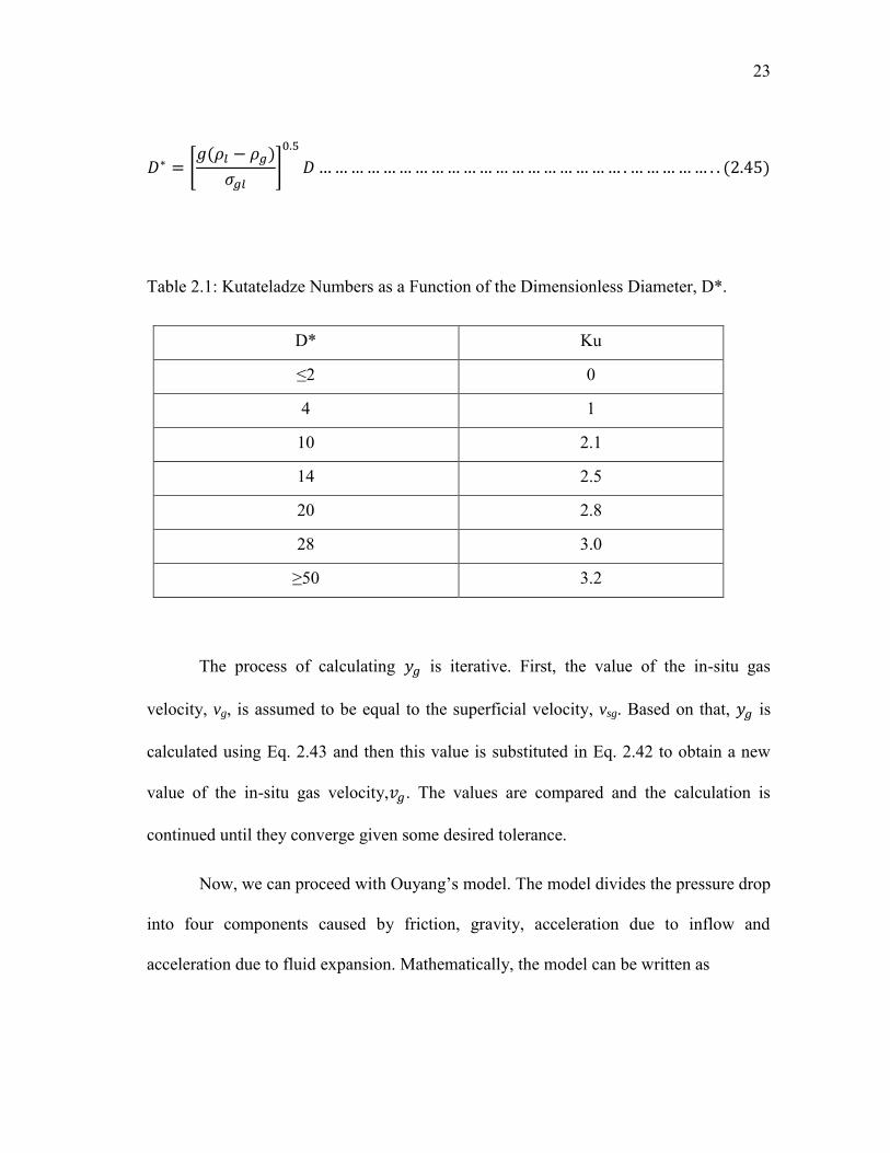
23

Table 2.1: Kutateladze Numbers as a Function of the Dimensionless Diameter, D*.

D* Ku

≤2 0

4 1

10 2.1

14 2.5

20 2.8

28 3.0

≥50 3.2

The process of calculating is iterative. First, the value of the in-situ gas

velocity, vg, is assumed to be equal to the superficial velocity, vsg. Based on that, is

calculated using Eq. 2.43 and then this value is substituted in Eq. 2.42 to obtain a new

value of the in-situ gas velocity, . The values are compared and the calculation is

continued until they converge given some desired tolerance.

Now, we can proceed with Ouyang’s model. The model divides the pressure drop

into four components caused by friction, gravity, acceleration due to inflow and

acceleration due to fluid expansion. Mathematically, the model can be written as

24

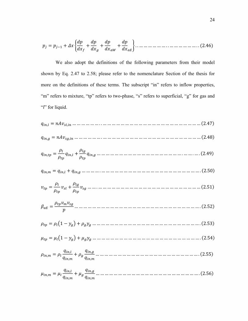
We also adopt the definitions of the following parameters from their model

shown by Eq. 2.47 to 2.58; please refer to the nomenclature Section of the thesis for

more on the definitions of these terms. The subscript “in” refers to inflow properties,

“m” refers to mixture, “tp” refers to two-phase, “s” refers to superficial, “g” for gas and

“l” for liquid.

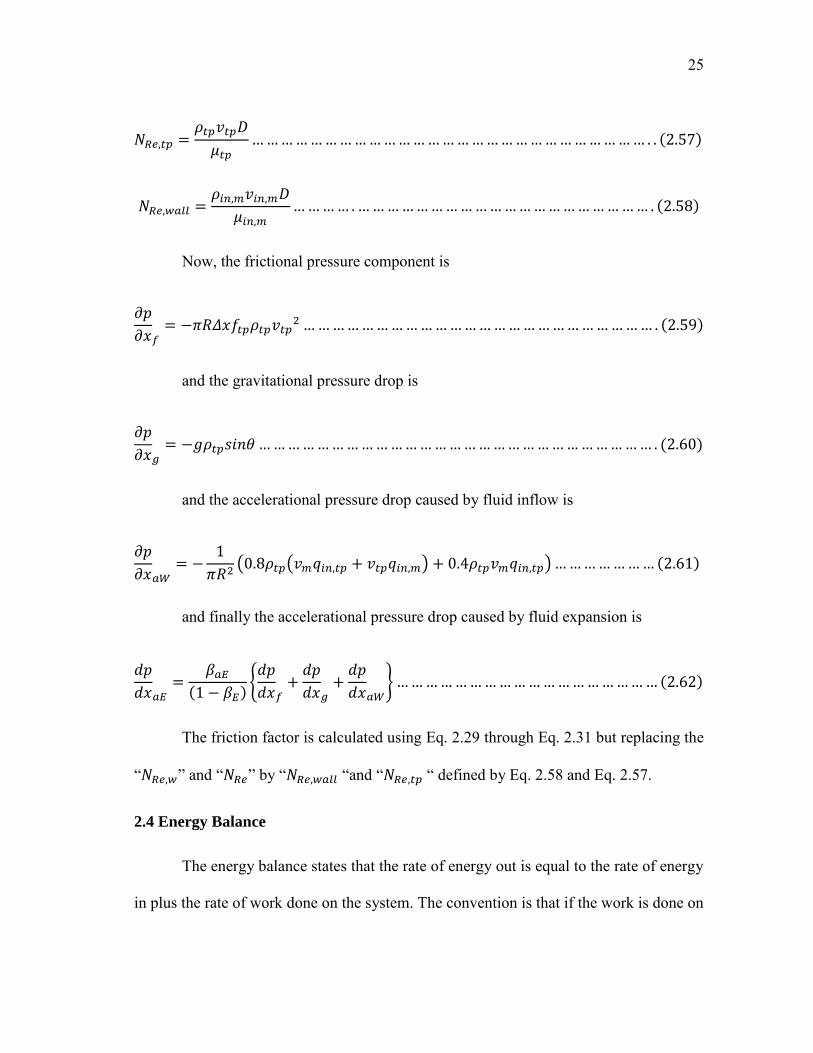
25

Now, the frictional pressure component is

and the gravitational pressure drop is

and the accelerational pressure drop caused by fluid inflow is

and finally the accelerational pressure drop caused by fluid expansion is

The friction factor is calculated using Eq. 2.29 through Eq. 2.31 but replacing the

“ ” and “ ” by “ “and “ “ defined by Eq. 2.58 and Eq. 2.57.

2.4 Energy Balance

The energy balance states that the rate of energy out is equal to the rate of energy

in plus the rate of work done on the system. The convention is that if the work is done on

26

the system then it is positive and if it is done by the system then it is negative and the

system loses energy.

2.4.1 Single Phase Flow

In the following derivation, we assume steady-state condition and we neglect the

heat conduction in fluid and the effect of gravity since we consider horizontal or near

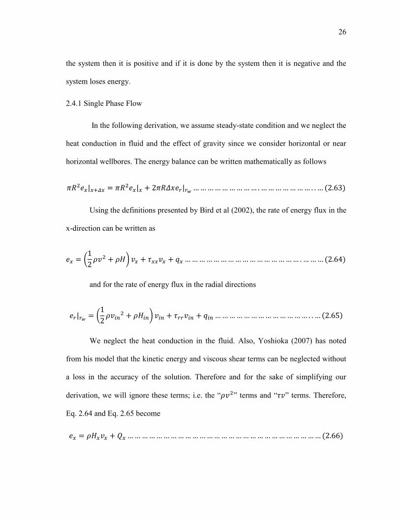
horizontal wellbores. The energy balance can be written mathematically as follows

Using the definitions presented by Bird et al (2002), the rate of energy flux in the

x-direction can be written as

and for the rate of energy flux in the radial directions

We neglect the heat conduction in the fluid. Also, Yoshioka (2007) has noted

from his model that the kinetic energy and viscous shear terms can be neglected without

a loss in the accuracy of the solution. Therefore and for the sake of simplifying our

derivation, we will ignore these terms; i.e. the “ ” terms and “ ” terms. Therefore,

Eq. 2.64 and Eq. 2.65 become

27

where Qx and Qin are the rates of conductive heat fluxes and the subscripts indicate that

the first is the rate of heat flux along the x-direction and latter is the rate of heat flux

caused by the fluid inflow. The rate of conductive heat flux, Qx, is through the fluid and

as we indicated earlier we are going to assume that the conductive heat in the fluid is

negligible and can be ignored. Therefore, Qx wil be zero. On the other hand, Qin is the

rate of conductive heat flux between the formation and the fluid in the pipe caused by

the difference between the temperature in the pipe fluid and the temperature in the

formation adjacent to the wall of the pipe. Bird el al. (2002) showed a derivation for the

expression for the rate of heat flux as a function of the difference between the fluid

temperature and the wall temperate and the overall heat transfer coefficient as shown by

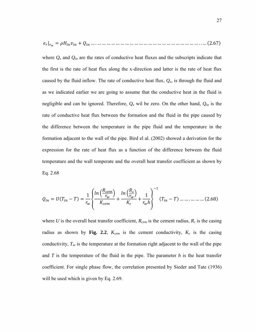
Eq. 2.68

where U is the overall heat transfer coefficient, Rcem is the cement radius, Rc is the casing

radius as shown by Fig. 2.2, Kcem is the cement conductivity, Kc is the casing

conductivity, Tin is the temperature at the formation right adjacent to the wall of the pipe

and T is the temperature of the fluid in the pipe. The parameter h is the heat transfer

coefficient. For single phase flow, the correlation presented by Sieder and Tate (1936)

will be used which is given by Eq. 2.69.

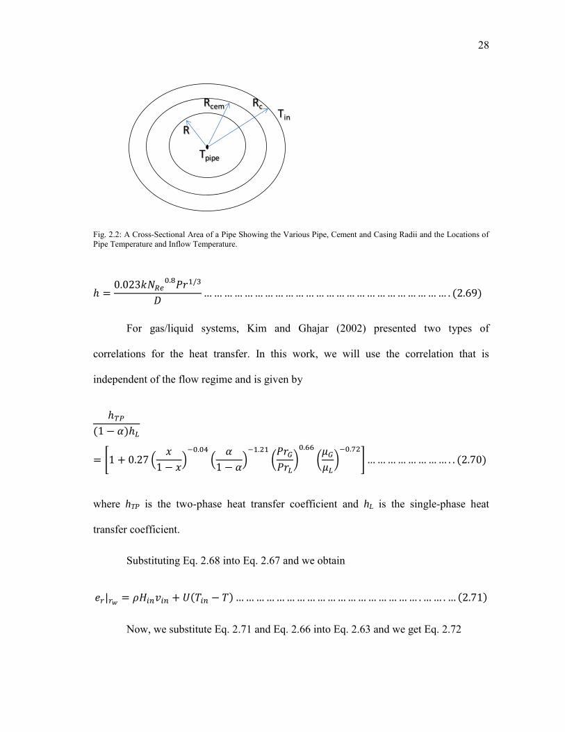
28

Fig. 2.2: A Cross-Sectional Area of a Pipe Showing the Various Pipe, Cement and Casing Radii and the Locations of Pipe Temperature and Inflow Temperature.

For gas/liquid systems, Kim and Ghajar (2002) presented two types of

correlations for the heat transfer. In this work, we will use the correlation that is

independent of the flow regime and is given by

where hTP is the two-phase heat transfer coefficient and hL is the single-phase heat

transfer coefficient.

Substituting Eq. 2.68 into Eq. 2.67 and we obtain

Now, we substitute Eq. 2.71 and Eq. 2.66 into Eq. 2.63 and we get Eq. 2.72

Tpipe

Tin

RcRcem

R

29

We note that in Eq. 2.72, we multiply the term by the segment open wall

area, using the variable γ, and we multiply the term representing the heat conduction by

the segment closed wall area, using the term (1-γ).

Now we rearrange Eq. 2.72, divide by ” and take the limit as

approaches zero to get the following differential form

To come up with a workable version of Eq. 2.73, we further expand the left hand

side as follows using chain rule

Now we will expand the terms Hx and vx more as follows. The enthalpy is

defined as

The specific volume, , is the inverse of density and the thermal expansion

coefficient is defined by Eq. 2.76

30

Therefore, we can write Eq. 2.75 as the following

We expand the term

using chain rule and incorporate the definition of

thermal expansion and we end up with Eq. 2.78

The superscripts indicate the value of the property at standard conditions. The

derivative of enthalpy then becomes

Moreover, Eq. 2.8 in a differential form becomes

Substituting (2.80) and (2.79) into (2.74) we obtain

Substituting equations (2.81) and (2.73) we get

31

Solving for the temperature derivative we get,

Using equation (2.75) for the definition of enthalpy, and assuming that the

pressure at the wall is the same as the pressure in the pipe, we end up with Eq. 2.84

Substituting (2.84) into (2.83) we obtain

Rearranging and combining similar terms, the final form becomes

We define a combined overall heat transfer coefficient that accounts for both the

heat conduction through the pipe and heat convection by inflow fluid as shown by Eq.

2.87

32

Joule-Thompson coefficient is defined by Eq. 2.88

Substituting Eq. 2.87 and Eq. 2.88 into Eq. 2.86, we obtain

For our modeling purpose, we will use the finite difference to discretize the

equation above. To simplify the manipulation process, we will introduce the following

variables

Therefore, equation (2.89) becomes

Solving for “ ” we obtain

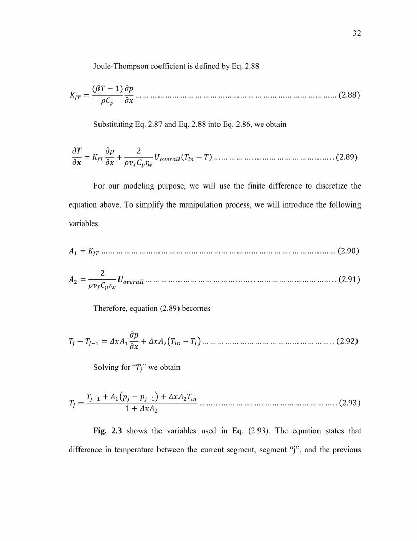
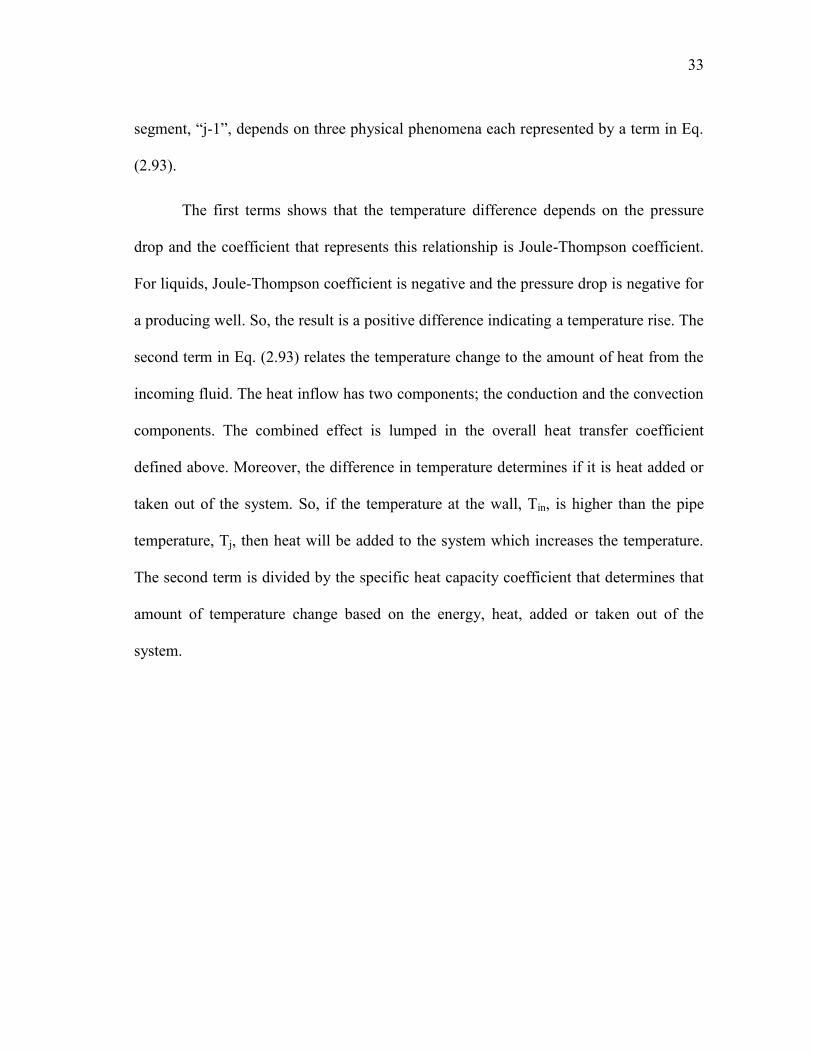
Fig. 2.3 shows the variables used in Eq. (2.93). The equation states that

difference in temperature between the current segment, segment “j”, and the previous

33

segment, “j-1”, depends on three physical phenomena each represented by a term in Eq.

(2.93).

The first terms shows that the temperature difference depends on the pressure

drop and the coefficient that represents this relationship is Joule-Thompson coefficient.

For liquids, Joule-Thompson coefficient is negative and the pressure drop is negative for

a producing well. So, the result is a positive difference indicating a temperature rise. The

second term in Eq. (2.93) relates the temperature change to the amount of heat from the

incoming fluid. The heat inflow has two components; the conduction and the convection

components. The combined effect is lumped in the overall heat transfer coefficient

defined above. Moreover, the difference in temperature determines if it is heat added or

taken out of the system. So, if the temperature at the wall, Tin, is higher than the pipe

temperature, Tj, then heat will be added to the system which increases the temperature.

The second term is divided by the specific heat capacity coefficient that determines that

amount of temperature change based on the energy, heat, added or taken out of the

system.

34

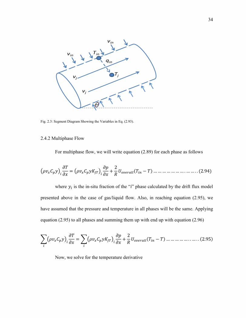
Fig. 2.3: Segment Diagram Showing the Variables in Eq. (2.93).

2.4.2 Multiphase Flow

For multiphase flow, we will write equation (2.89) for each phase as follows

where is the in-situ fraction of the “i” phase calculated by the drift flux model

presented above in the case of gas/liquid flow. Also, in reaching equation (2.95), we

have assumed that the pressure and temperature in all phases will be the same. Applying

equation (2.95) to all phases and summing them up with end up with equation (2.96)

Now, we solve for the temperature derivative

vj

vin

Tj

Tin

vj

qin

vin

35

We define the following variables

The final discrete form is

36

3. RESERVOIR MODEL

3.1 Introduction

As with the wellbore model, there are two equations we are interested in, the

reservoir pressure and temperature models. These models have derived by Furui (2003),

Dawkrajai (2006) and Yoshioka (2007) and in this Section we summarize their

assumptions and results.

3.2 Reservoir Pressure Model

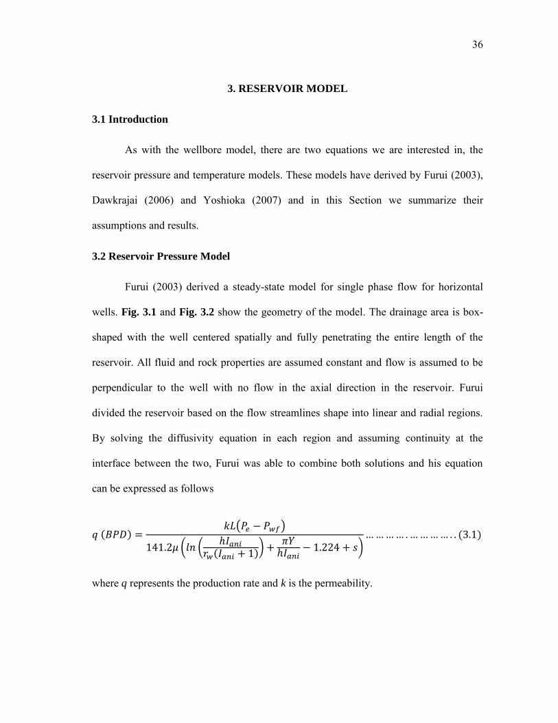
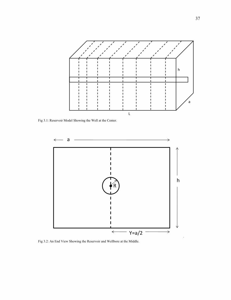
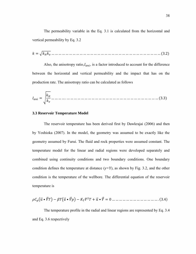
Furui (2003) derived a steady-state model for single phase flow for horizontal

wells. Fig. 3.1 and Fig. 3.2 show the geometry of the model. The drainage area is box-

shaped with the well centered spatially and fully penetrating the entire length of the

reservoir. All fluid and rock properties are assumed constant and flow is assumed to be

perpendicular to the well with no flow in the axial direction in the reservoir. Furui

divided the reservoir based on the flow streamlines shape into linear and radial regions.

By solving the diffusivity equation in each region and assuming continuity at the

interface between the two, Furui was able to combine both solutions and his equation

can be expressed as follows

where q represents the production rate and k is the permeability.

37

Fig 3.1: Reservoir Model Showing the Well at the Center.

. Fig 3.2: An End View Showing the Reservoir and Wellbore at the Middle.

h

a

L

a

h

Y=a/2

R

38

The permeability variable in the Eq. 3.1 is calculated from the horizontal and

vertical permeability by Eq. 3.2

Also, the anisotropy ratio, , is a factor introduced to account for the difference

between the horizontal and vertical permeability and the impact that has on the

production rate. The anisotropy ratio can be calculated as follows

3.3 Reservoir Temperature Model

The reservoir temperature has been derived first by Dawkrajai (2006) and then

by Yoshioka (2007). In the model, the geometry was assumed to be exactly like the

geometry assumed by Furui. The fluid and rock properties were assumed constant. The

temperature model for the linear and radial regions were developed separately and

combined using continuity conditions and two boundary conditions. One boundary

condition defines the temperature at distance (y=Y), as shown by Fig. 3.2, and the other

condition is the temperature of the wellbore. The differential equation of the reservoir

temperature is

The temperature profile in the radial and linear regions are represented by Eq. 3.4

and Eq. 3.6 respectively

39

where “y” is the distance in the linear region of the reservoir and it goes from

y=h/2 to y=a/2, which is half the width.

The following is a list of the variables needed to evaluate the equations above

40

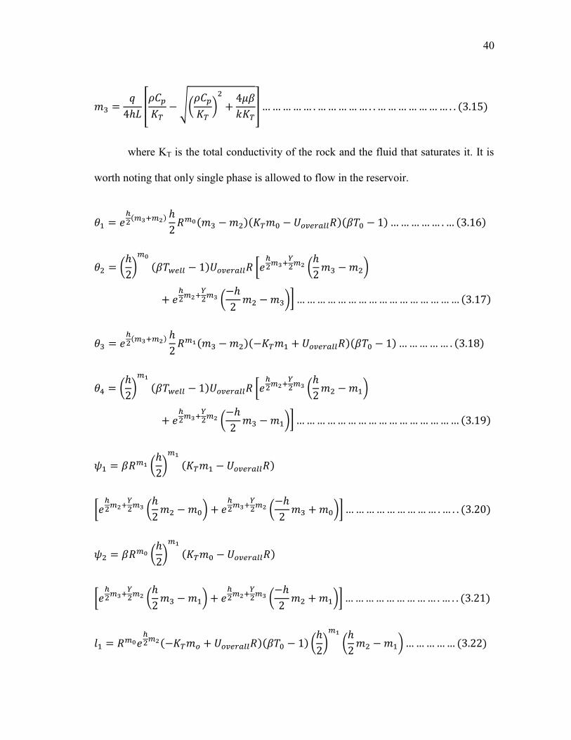
where KT is the total conductivity of the rock and the fluid that saturates it. It is

worth noting that only single phase is allowed to flow in the reservoir.

41

42

4. COUPLED WELLBORE AND RESERVOIR MODEL

4.1 Introduction

The objective of this research is to develop a model that couples the flow from

two or three horizontal laterals into one motherbore as shown by Fig. 4.1. The program

will calculate the pressure and temperature profiles along the motherbore in multilateral

wells. In the following Sections, we describe the development of this model.

4.1.1 Multilateral Well Model Assumptions

First of all, we start by explaining the geometry and terminology that will be used

for the model. Fig. 4.1 is top view diagram of a trilateral well. As we can see, the three

horizontal wellbores, or laterals, are connected to one main conduit or a motherbore at

the subsurface level. The individual horizontal laterals are shown by the dotted green

rectangles and lines and their respective drainage areas are shown by dotted orange

rectangles. As we explained in Section Three, the drainage areas will be boxed-shaped in

three-dimensional frame work. It is worth mentioning that these orange rectangles are

not connected which signifies the assumption that the laterals drain separate and non-

communicating reservoirs.

As shown by the legends in Fig. 4.1, the blue boxes represent the packers which

prevent the fluid to flow in the annulus between the tubing and the casing forcing the

flow to go into the tubing. The red circles represent the inflow choke valves which can

be adjusted to restrict the flow from a certain lateral or to eliminate the production from

that lateral completely. The arrows show the direction of flow in the system.

43

Fig. 4.1: A Diagram of Three Laterals Connected to a Motherbore that Shows the Segmentations, the Location of The Valves and Packers.

Throughout this thesis, regarding a horizontal lateral, a toe segment is the one

furthest away from the motherbore and a heel segment is the one adjacent and connected

to the motherbore as shown by lateral #3 in Fig 4.1.

Lateral #1“L1”

Motherbore“MB”

123Max #

1

2

Max #

12

Ma

x #

Max #

Lateral #3“L3”

Lateral #2“L2”

PackersICVInternal Control Valves

Toe

Heel

Jun#1Jun#2

ICVInternal Control Valves

Packers

Casing

Tubing

44

In our model, each lateral is treated like a separate horizontal well. That is, the

reservoir is segmented as shown by Fig. 3.1 and Fig. 4.1 so that only one phase is

allowed to flow in each segment. However, different segments can have different phases

flowing. One reservoir segment can flow oil and the other segment can flow water and

multiphase flow can occur in the wellbore.

Moreover, the reservoir model assumes that the drainage area for each lateral is

defined and in our model we will assume that the information is provided as an input. It

is also assumed that the laterals do not interfere with each other in the reservoir. This

assumption holds correct if laterals are drilled in different, non-communicating

formations. The assumption is reasonable when laterals are drilled far apart from each

other so that inference effect can be neglected. When all the laterals are allowed to

produce, their production is commingled in the motherbore and that is how a lateral’s

performance can affect other laterals’ production. For example, laterals drilled in high

pressure reservoirs will tend to choke the production for other laterals and dominate the

flow.

The rock properties are assumed to be provided by the user and are assumed to

be constant throughout the calculation. Also, the fluid properties can either be provided

by the user or calculated from common correlations in the petroleum literature presented

by McCain (1990) and Prats (1982). The properties will be given, or calculated, at

average pressure and temperature values that are expected for a specific run and will

then be assumed constant throughout the calculation.

45

As we have indicated, the aim of the study is to calculate the pressure and

temperature profile along the motherbore. The laterals and the motherbore are assumed

to be horizontal or near horizontal with only slight inclination. Therefore, there will be a

slight temperature variation which should not alter the properties significantly.

Moreover, the reservoir pressure in all the cases that we consider is above 2,500 psi and

the pressure change in the reservoir will be mostly between 100 -200 psi with the

exception of two runs where the drawdown pressure was 300 psi. Under these

conditions, the change in the oil and water properties will not be significant and is

assumed to have negligible effect on the results.

4.2 Coupled Pressure Model

The solution process starts with solving for the pressure in each lateral and in the

motherbore. The process is illustrated by Fig. 4.2 and starts by assuming a pressure

profile in the first lateral, L1. Based on Eq. 3.1, the inflow rates are calculated. After

that, if multiphase flow exists, then we calculate the fraction of each phase using Eq.

2.35 through Eq. 2.37 for oil/water system. If we deal with gas/liquid flow, then Eq. 2.40

through Eq. 2.45 are used to estimate the in-situ gas and liquid fractions.

After that, we calculate the pressure drop in the lateral. To do so, we use Eq.

2.28 for single phase, Eq. 2.39 for oil/water two-phase flow or Ouyang’s model for

gas/liquid flow represented by Eq. 2.46 through Eq. 2.62. Once the pressure drop is

calculated, a new pressure profile will be obtained. The new pressure profile is compared

to initial assumed profile, if both profiles converge, given a desired tolerance, then the

process is terminated. Otherwise, the new pressure profile is used to calculate the inflow

46

rates and process is repeated until convergence is achieved. This procedure is illustrated

by Fig. 4.2. Eq. 4.1 shows the convergence criteria used in our calculation.

where “p” is the pressure vector representing the wellbore pressure and the superscripts

indicate the different iterations.

47

Fig. 4.2: Pressure Calculation Process in Each Lateral.

Assign P profile for L1, P „

Calculate inflow rateEq. 3.1

Estimate holdupEq. 2.40 – Eq. 2.45

Calculate pressure drop in wellboreEq. 2.28 for single phase

Eq. 2.39 or Eq. 2.46 for two-phase

P „ & P “ converge ?

Calculate P drop across ICVEq. 4.2

No

Yes

Obtain a new P profile for L1, P “

48

The total flow from L1 enters the wellbore at the toe of the motherbore, shown as

segment #1 in Fig. 4.1. The flow rate is the total flow rate for each phase from all

segments but we still have to calculate the pressure at the toe of the motherbore. As the

flow enters the motherbore, it passes through the ICV, or the inflow control valve, where

it is subjected to a pressure drop. These valves open in an incremental fashion going

from position one to ten with each position having a different open area. To estimate the

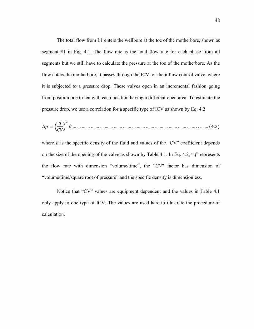
pressure drop, we use a correlation for a specific type of ICV as shown by Eq. 4.2

where is the specific density of the fluid and values of the “CV” coefficient depends

on the size of the opening of the valve as shown by Table 4.1. In Eq. 4.2, “q” represents

the flow rate with dimension “volume/time”, the “CV” factor has dimension of

“volume/time/square root of pressure” and the specific density is dimensionless.

Notice that “CV” values are equipment dependent and the values in Table 4.1

only apply to one type of ICV. The values are used here to illustrate the procedure of

calculation.

49

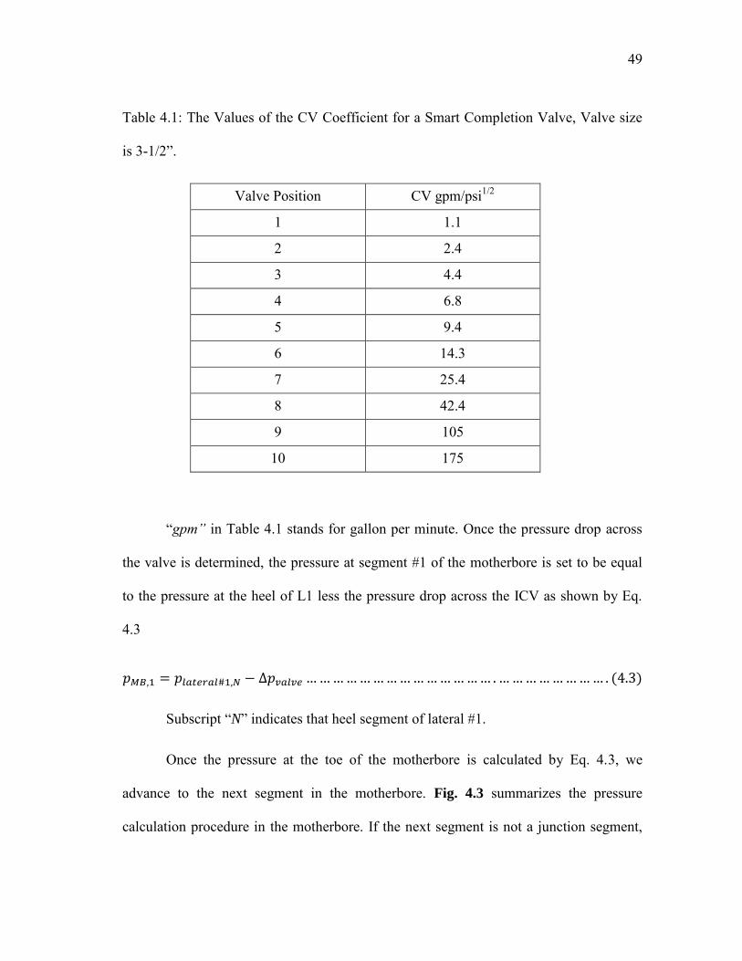
Table 4.1: The Values of the CV Coefficient for a Smart Completion Valve, Valve size

is 3-1/2”.

Valve Position CV gpm/psi1/2

1 1.1

2 2.4

3 4.4

4 6.8

5 9.4

6 14.3

7 25.4

8 42.4

9 105

10 175

“gpm” in Table 4.1 stands for gallon per minute. Once the pressure drop across

the valve is determined, the pressure at segment #1 of the motherbore is set to be equal

to the pressure at the heel of L1 less the pressure drop across the ICV as shown by Eq.

4.3

Subscript “N” indicates that heel segment of lateral #1.

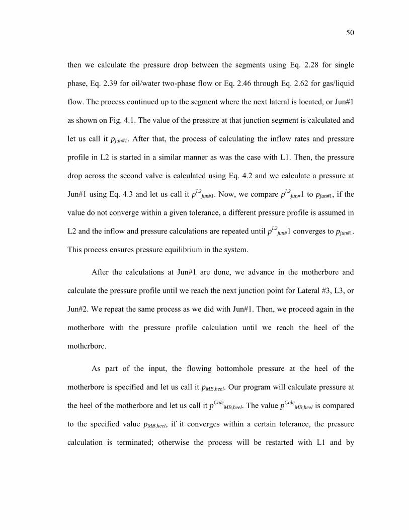
Once the pressure at the toe of the motherbore is calculated by Eq. 4.3, we

advance to the next segment in the motherbore. Fig. 4.3 summarizes the pressure

calculation procedure in the motherbore. If the next segment is not a junction segment,

50

then we calculate the pressure drop between the segments using Eq. 2.28 for single

phase, Eq. 2.39 for oil/water two-phase flow or Eq. 2.46 through Eq. 2.62 for gas/liquid

flow. The process continued up to the segment where the next lateral is located, or Jun#1

as shown on Fig. 4.1. The value of the pressure at that junction segment is calculated and

let us call it pjun#1. After that, the process of calculating the inflow rates and pressure

profile in L2 is started in a similar manner as was the case with L1. Then, the pressure

drop across the second valve is calculated using Eq. 4.2 and we calculate a pressure at

Jun#1 using Eq. 4.3 and let us call it pL2jun#1. Now, we compare pL2

jun#1 to pjun#1, if the

value do not converge within a given tolerance, a different pressure profile is assumed in

L2 and the inflow and pressure calculations are repeated until pL2jun#1 converges to pjun#1.

This process ensures pressure equilibrium in the system.

After the calculations at Jun#1 are done, we advance in the motherbore and

calculate the pressure profile until we reach the next junction point for Lateral #3, L3, or

Jun#2. We repeat the same process as we did with Jun#1. Then, we proceed again in the

motherbore with the pressure profile calculation until we reach the heel of the

motherbore.

As part of the input, the flowing bottomhole pressure at the heel of the

motherbore is specified and let us call it pMB,heel. Our program will calculate pressure at

the heel of the motherbore and let us call it pCalcMB,heel. The value pCalc

MB,heel is compared

to the specified value pMB,heel, if it converges within a certain tolerance, the pressure

calculation is terminated; otherwise the process will be restarted with L1 and by

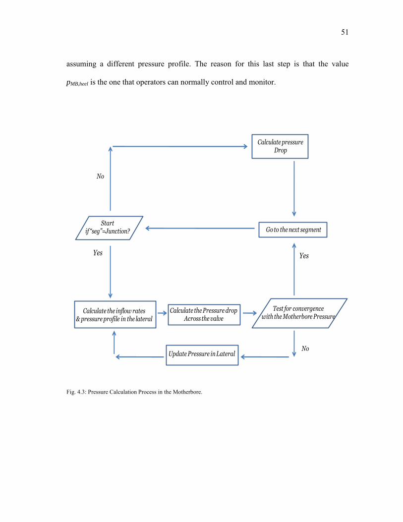
51

assuming a different pressure profile. The reason for this last step is that the value

pMB,heel is the one that operators can normally control and monitor.

Fig. 4.3: Pressure Calculation Process in the Motherbore.

Startif “seg”=Junction?

Yes

No

Calculate pressureDrop

Calculate the inflow rates& pressure profile in the lateral

Go to the next segment

Calculate the Pressure dropAcross the valve

Test for convergencewith the Motherbore Pressure

Update Pressure in Lateral

Yes

No

52

4.3 Coupled Temperature Model

4.3.1: Temperature Calculation in Each Lateral

Once the pressure profiles are calculated in the motherbore and in each lateral,

we then proceed with calculating the temperature profile in the system. We first start

with L1 and from the toe segment, segment #1. In Sections 2 and 3, we derived the

wellbore and temperature models represented by Eq. 2.94 for single phase and Eq. 2.101

for multiphase. We also showed the equation for the reservoir temperature model

represented by Eq. 3.6. These equations are shown below for reference.

In our model, we need to calculate the temperature at the wall of the lateral

which is Tin in our notation. Therefore, Eq. (3.6) is evaluated at a distance equivalent to

the wellbore radius, rw. Also, we note that the wellbore temperature, Tj, is a function of

the fluid properties in the pipe, wellbore geometry and the reservoir inflow temperature,

Tin as shown by Eq. 2.94 and Eq. 2.101. Also, the reservoir inflow temperature, Tin, is a

function of the reservoir fluid properties, the inflow rate, reservoir geometry and the

wellbore temperature at each segment, i.e. Tj, as shown by Eq. 3.6. Eq. 3.6 does not

show the dependency on the wellbore temperature however the calculation of the

53

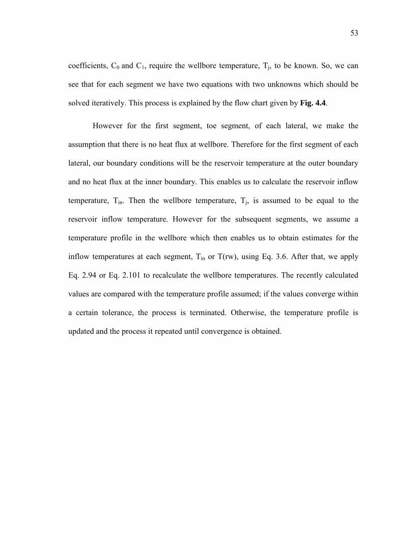
coefficients, C0 and C1, require the wellbore temperature, Tj, to be known. So, we can

see that for each segment we have two equations with two unknowns which should be

solved iteratively. This process is explained by the flow chart given by Fig. 4.4.

However for the first segment, toe segment, of each lateral, we make the

assumption that there is no heat flux at wellbore. Therefore for the first segment of each

lateral, our boundary conditions will be the reservoir temperature at the outer boundary

and no heat flux at the inner boundary. This enables us to calculate the reservoir inflow

temperature, Tin. Then the wellbore temperature, Tj, is assumed to be equal to the

reservoir inflow temperature. However for the subsequent segments, we assume a

temperature profile in the wellbore which then enables us to obtain estimates for the

inflow temperatures at each segment, Tin or T(rw), using Eq. 3.6. After that, we apply

Eq. 2.94 or Eq. 2.101 to recalculate the wellbore temperatures. The recently calculated

values are compared with the temperature profile assumed; if the values converge within

a certain tolerance, the process is terminated. Otherwise, the temperature profile is

updated and the process it repeated until convergence is obtained.

54

Fig. 4.4: Wellbore Temperature Calculation Procedure in Each Lateral.

As we have shown in the pressure model calculation, there will be a pressure

drop across the smart completion valve and an associated temperature rise or drop

depending on the fluid type. To calculate this temperature change across the valve, we

use Eq. 4.3 for single phase flow or we use Eq. 4.4 to calculate the associated

temperature change for multiphase flow. In these equations, we use Joule-Thompson

coefficient to convert the pressure drop into a temperature change.

Calculate TemperatureIn first segment

Assign T Profile for the lateral

Calculate reservoir inflow temperaturesEq. 3.6

Calculate a new wellbore temperature profileEq. 2.94 for single phaseEq. 2.101 for multiphase

T converged ?

Calculate T Change across ICV

No

Yes

55

For single phase;

For multiphase phase;

4.3.2: Temperature Calculation in the Motherbore

The temperature profile in the motherbore is calculated after the temperature

profile in each lateral is determined. The calculation is started from the toe of the

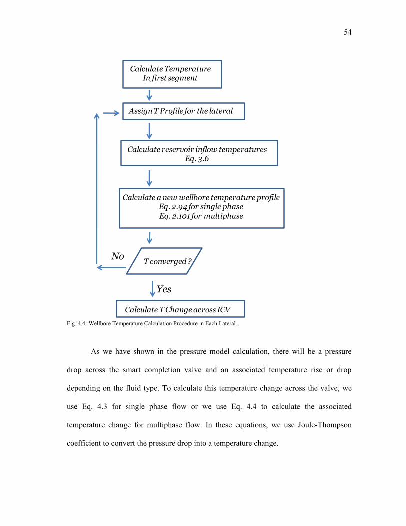
motherbore, lowest segment. As shown by Fig. 4.5, the flow rate, pressure and

temperature have been determined at the heel of lateral #1, L1. To calculate the

temperature at the first segment in the motherbore, we add the temperature change

across the valve to the temperature at the heel of lateral #1, or L1. This temperature

change is caused by the pressure drop and is calculated using Eq. 4.3 or Eq. 4.4.

56

Fig. 4.5: Diagram Showing the Calculation Variables for the First Segment in the Motherbore.

For the subsequent segments in the motherbore, Eq. 2.94 or Eq. 2.101 is used for

single phase flow or multiphase flow respectively and the inflow terms are dropped since

there is no inflow. For example, Eq. (2.94) becomes

Eq. (4.5) shows that the temperature rise between any two segments will be

mainly caused by the pressure drop between the segments.

For the segments that are junction points; that is, segments where laterals

intersect the motherbore, we apply Eq. 2.94 or Eq. 2.101 however with some

modifications to the variables used. As shown by Fig. 4.6, variables with subscript “L”

indicate that the value is calculated for the lateral and variables with subscript “M”

indicate that the value is calculated for the motherbore. Subscripts “j” and “j-1” indicate

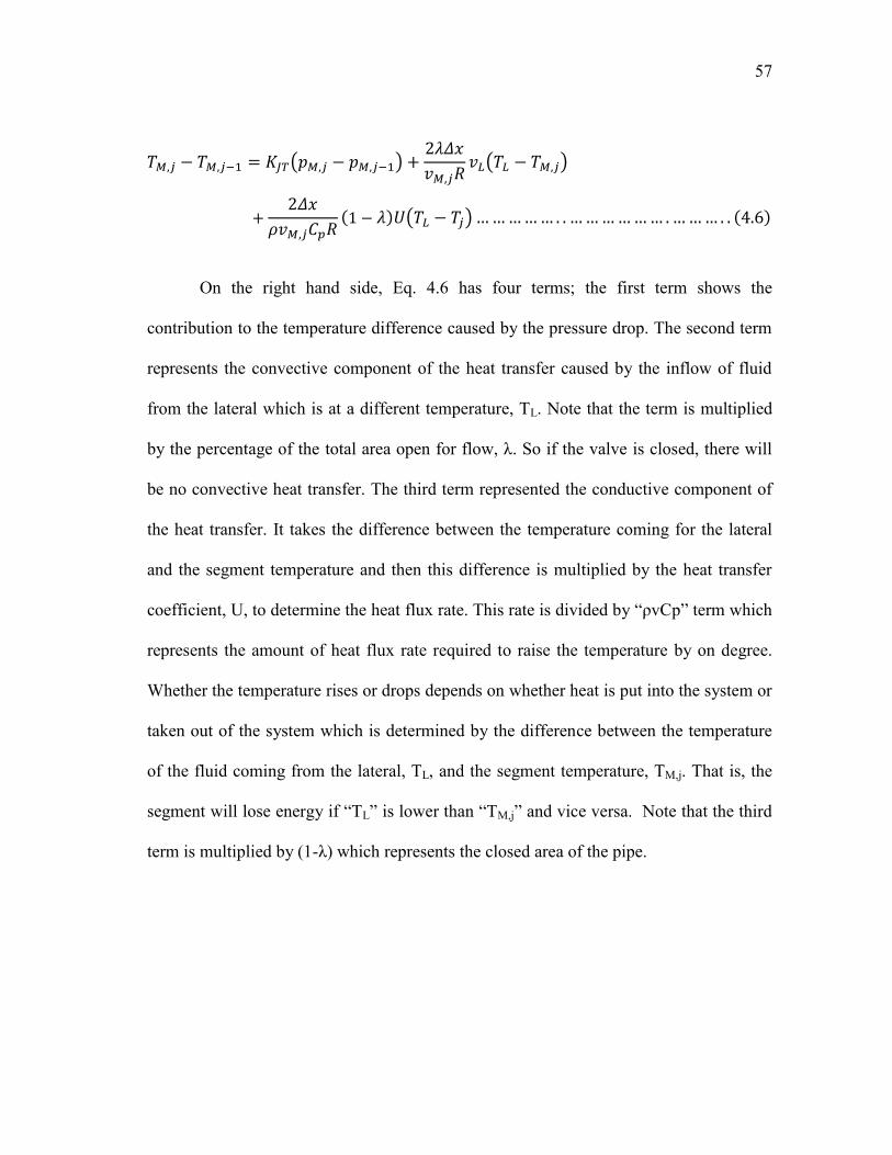
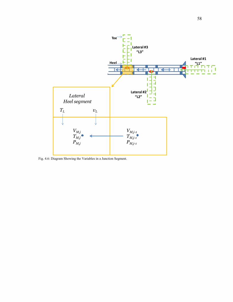
a segment and its predecessor. Eq. 4.6 shows the form of the equation used.

Lateral #1 Heel SegmentMotherbore First SegmentTj

Pj

Q j

T1 =Tj+∆T(valve)P1 =Pj+∆P(valve)Q1= Q j

Smart Completion Valve

57

On the right hand side, Eq. 4.6 has four terms; the first term shows the

contribution to the temperature difference caused by the pressure drop. The second term

represents the convective component of the heat transfer caused by the inflow of fluid

from the lateral which is at a different temperature, TL. Note that the term is multiplied

by the percentage of the total area open for flow, λ. So if the valve is closed, there will

be no convective heat transfer. The third term represented the conductive component of

the heat transfer. It takes the difference between the temperature coming for the lateral

and the segment temperature and then this difference is multiplied by the heat transfer

coefficient, U, to determine the heat flux rate. This rate is divided by “ρvCp” term which

represents the amount of heat flux rate required to raise the temperature by on degree.

Whether the temperature rises or drops depends on whether heat is put into the system or

taken out of the system which is determined by the difference between the temperature

of the fluid coming from the lateral, TL, and the segment temperature, TM,j. That is, the

segment will lose energy if “TL” is lower than “TM,j” and vice versa. Note that the third

term is multiplied by (1-λ) which represents the closed area of the pipe.

58

Fig. 4.6: Diagram Showing the Variables in a Junction Segment.

Lateral #3“L3”

Lateral #2“L2”

Toe

HeelLateral #1

“L1”

TL vL

VM,j

TM,j

PM,j

VM,j-1

TM,j-1

PM,j-1

Lateral Heel segment

59

5. RESULTS AND DISCUSSION

5.1 Results for Horizontal Wells

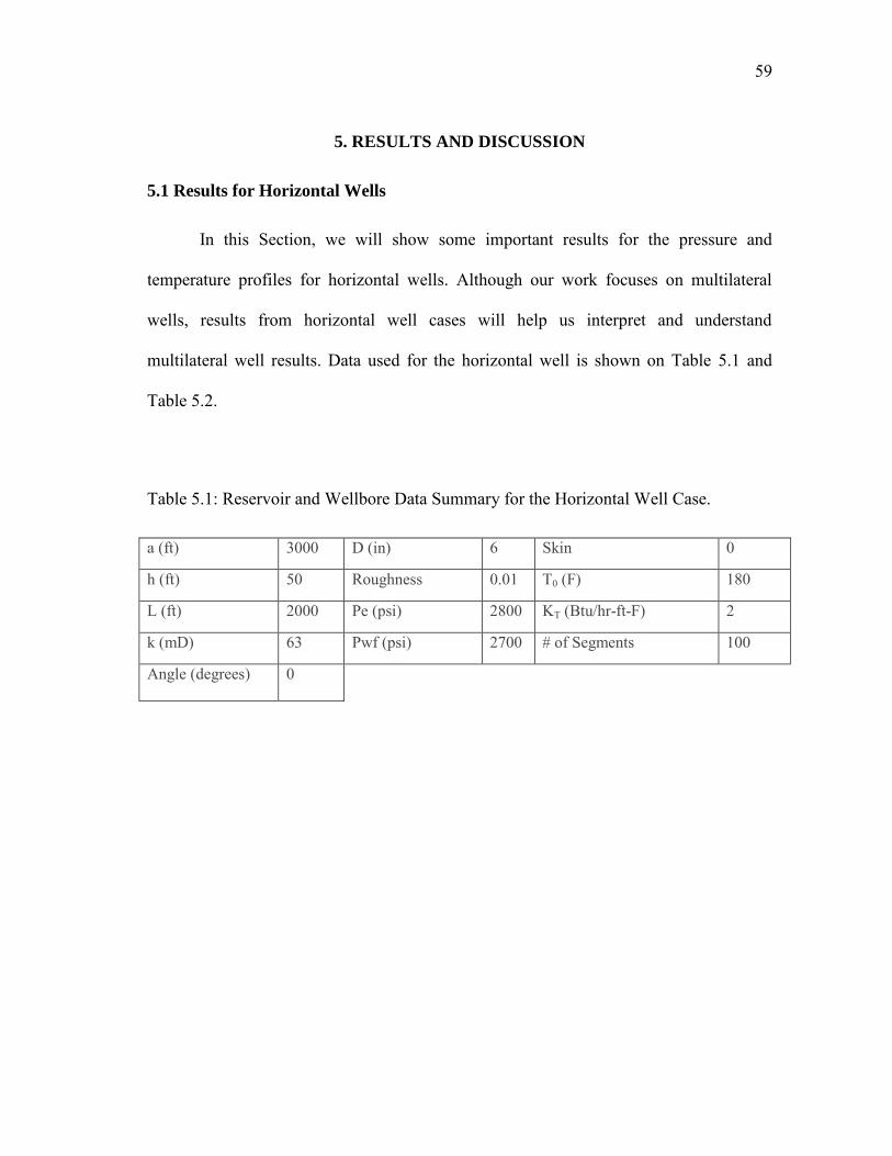
In this Section, we will show some important results for the pressure and

temperature profiles for horizontal wells. Although our work focuses on multilateral

wells, results from horizontal well cases will help us interpret and understand

multilateral well results. Data used for the horizontal well is shown on Table 5.1 and

Table 5.2.

Table 5.1: Reservoir and Wellbore Data Summary for the Horizontal Well Case.

a (ft) 3000 D (in) 6 Skin 0

h (ft) 50 Roughness 0.01 T0 (F) 180

L (ft) 2000 Pe (psi) 2800 KT (Btu/hr-ft-F) 2

k (mD) 63 Pwf (psi) 2700 # of Segments 100

Angle (degrees) 0

60

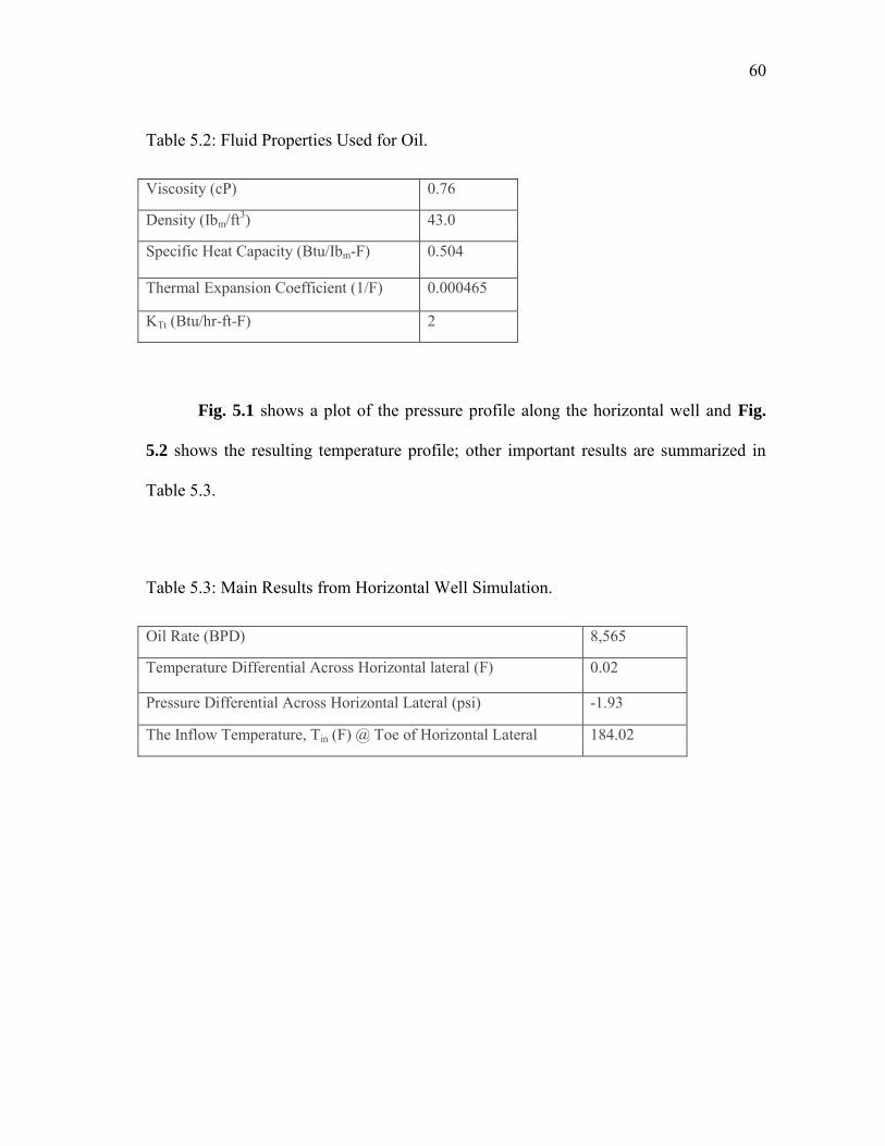
Table 5.2: Fluid Properties Used for Oil.

Viscosity (cP) 0.76

Density (Ibm/ft3) 43.0

Specific Heat Capacity (Btu/Ibm-F) 0.504

Thermal Expansion Coefficient (1/F) 0.000465

KTt (Btu/hr-ft-F) 2

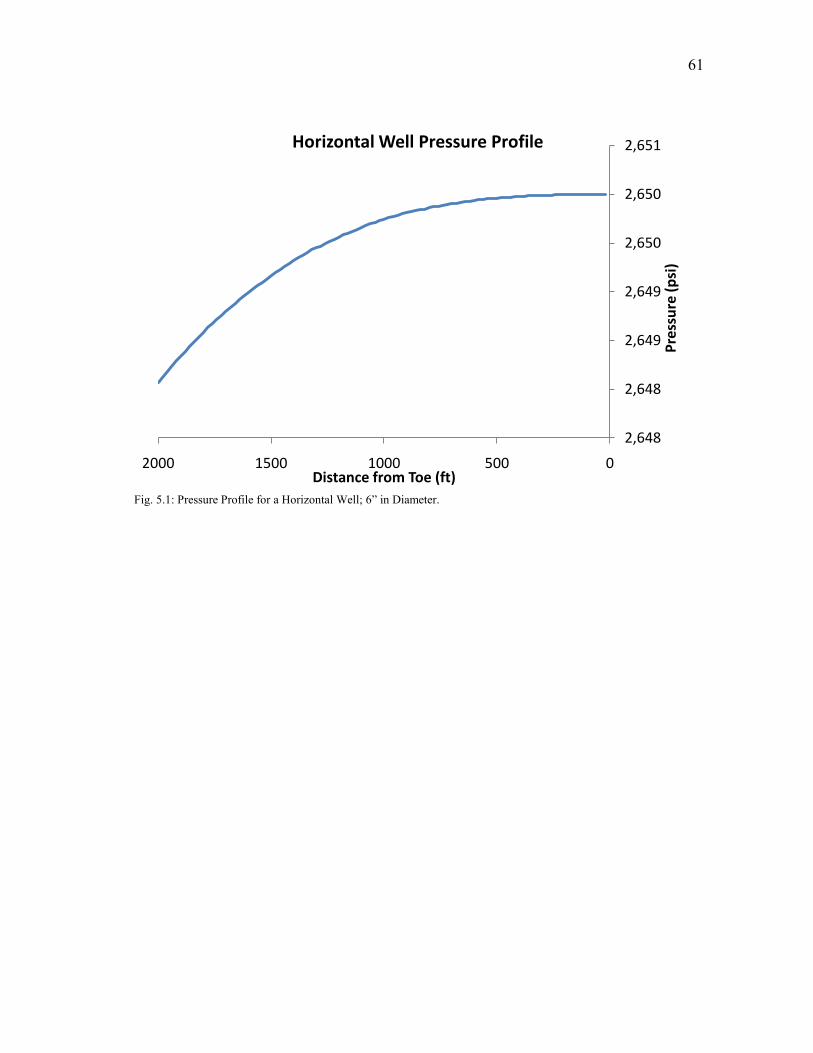
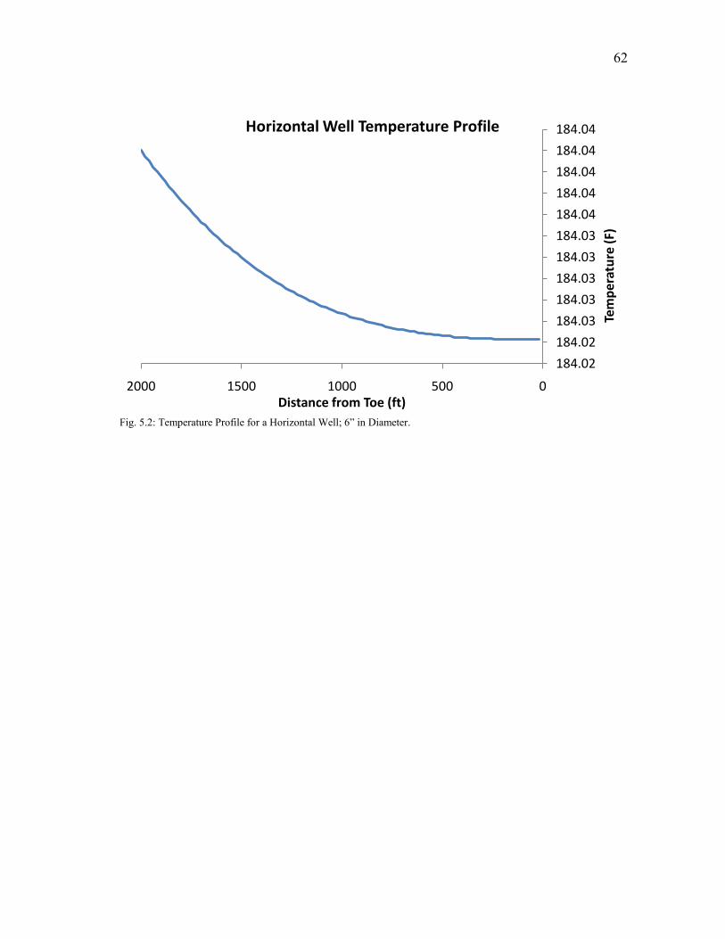
Fig. 5.1 shows a plot of the pressure profile along the horizontal well and Fig.

5.2 shows the resulting temperature profile; other important results are summarized in

Table 5.3.

Table 5.3: Main Results from Horizontal Well Simulation.

Oil Rate (BPD) 8,565

Temperature Differential Across Horizontal lateral (F) 0.02

Pressure Differential Across Horizontal Lateral (psi) -1.93

The Inflow Temperature, Tin (F) @ Toe of Horizontal Lateral 184.02

61

Fig. 5.1: Pressure Profile for a Horizontal Well; 6” in Diameter.

2,648

2,648

2,649

2,649

2,650

2,650

2,651

0500100015002000

Pre

ssu

re (

psi

)

Distance from Toe (ft)

Horizontal Well Pressure Profile

62

Fig. 5.2: Temperature Profile for a Horizontal Well; 6” in Diameter.

184.02

184.02

184.03

184.03

184.03

184.03

184.03

184.04

184.04

184.04

184.04

184.04

0500100015002000

Tem

per

atu

re (

F)

Distance from Toe (ft)

Horizontal Well Temperature Profile

63

We can see from this run that the temperature of the fluid flowing in the reservoir

heated up (4.02 F) arriving at the wellbore at a temperature of (184.02 F). This is the

incoming fluid temperature at the toe of the horizontal well which is equal to the

wellbore temperature at the toe segment as indicated in our assumptions earlier; please

refer to Section 4.3. This heating effect is expected since the Joule-Thompson

coefficient, which combines the effect of viscous dissipation and fluid expansion, is

negative for the oil and the pressure drop in the reservoir is negative and that results in a

rise in the temperature of the fluid as it flows in the reservoir.

Fig. 5.1 gives us typical pressure drops in wellbores. This case with 8,565 BPD,

we observe a pressure drop of only (1.93) psi. Moreover, the plot shows the effect of

inflow on the pressure drop. As we can see, the pressure drop increases as we go towards

the heel. That is because more fluid is entering the wellbore and the inflow rates increase

the friction factor, the mass in the system and the velocity.

Fig 5.2 also shows a typical increase in temperature in the wellbore. This slight

increase is a result of the small pressure drop experienced in the wellbore. The wellbore

is (6 inches) in diameter which is considered large. Typical wellbore diameters for

horizontal wells vary somewhere between (2.5 inches – 4 inches). Six inches diameter is

common with multilateral wells and this is the reason for our selection.

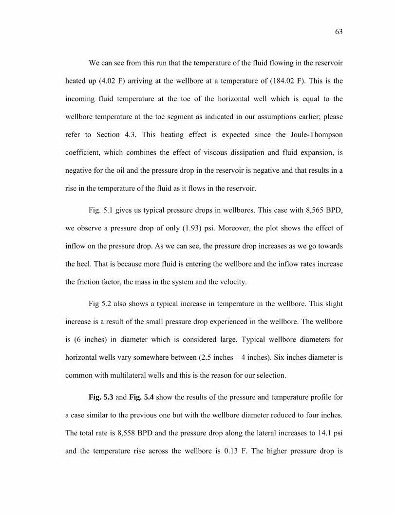
Fig. 5.3 and Fig. 5.4 show the results of the pressure and temperature profile for

a case similar to the previous one but with the wellbore diameter reduced to four inches.

The total rate is 8,558 BPD and the pressure drop along the lateral increases to 14.1 psi

and the temperature rise across the wellbore is 0.13 F. The higher pressure drop is

64

caused by the fact that the wellbore is smaller. The higher pressure drop caused the

temperature rise to be higher.

Fig. 5.3: Pressure Profile for a Horizontal Well; 4” in Diameter.

To understand the difference in pressure and temperature profiles when a

different phase is flowing, we will compare simulation runs for single phase oil and

single phase water. That is, we conduct three runs assuming that only the oil phase exists

and we vary the drawdown pressure. After that, we conduct the same runs but assuming

that only the water phase exists. The similarity will be in all geometrical aspects of

wellbore and reservoir as well as the pressure drawdown. Properties used for the water

are summarized in Table 5.4. The results of these runs are summarized in Table 5.5. The

Table shows that for both oil and water, the arriving inflow temperature is higher than

the geothermal temperature, which is 180 F, and that the fluid heats up in the wellbore as

2,634

2,636

2,638

2,640

2,642

2,644

2,646

2,648

2,650

2,652

0500100015002000

Pre

ssu

re (

psi

)

Distance from Toe (ft)

Horizontal Well Pressure Profile, 4" Diameter

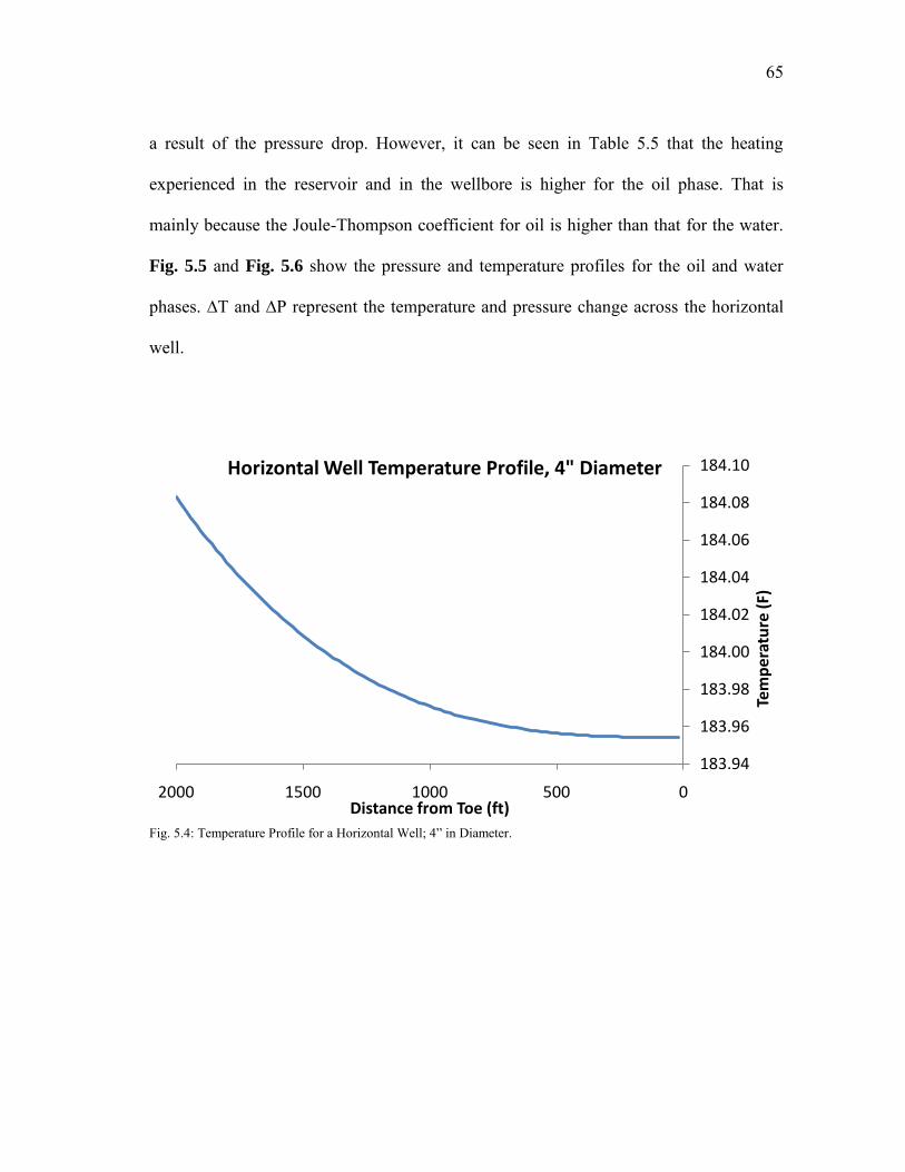
65

a result of the pressure drop. However, it can be seen in Table 5.5 that the heating

experienced in the reservoir and in the wellbore is higher for the oil phase. That is

mainly because the Joule-Thompson coefficient for oil is higher than that for the water.

Fig. 5.5 and Fig. 5.6 show the pressure and temperature profiles for the oil and water

phases. ∆T and ∆P represent the temperature and pressure change across the horizontal

well.

Fig. 5.4: Temperature Profile for a Horizontal Well; 4” in Diameter.

183.94

183.96

183.98

184.00

184.02

184.04

184.06

184.08

184.10

0500100015002000

Tem

per

atu

re (

F)

Distance from Toe (ft)

Horizontal Well Temperature Profile, 4" Diameter

66

Table 5.4: Fluid Properties Used for Water.

Viscosity (cP) 0.48

Density (Ibm/ft3) 63.04

Specific Heat Capacity (Btu/Ibm-F) 1.002

Thermal Expansion Coefficient (1/F) 0.000311

Conductivity (Btu/hr-ft-F) 2.5

Table 5.5: Summary of Oil and Water Runs at Different Drawdown Pressures.

Phase Drawdown

Pressure (psi)

Diameter

(in) Tin (F) ∆T (F) ∆P (psi

Oil 300 6 188.14 0.07 -7.7

Oil 200 6 185.40 0.03 -3.4

Oil 100 6 182.65 0.01 -0.9

Water 300 6 183.16 0.10 -28.6

Water 200 6 182.08 0.05 -12.6

Water 100 6 181.01 0.01 -3.14

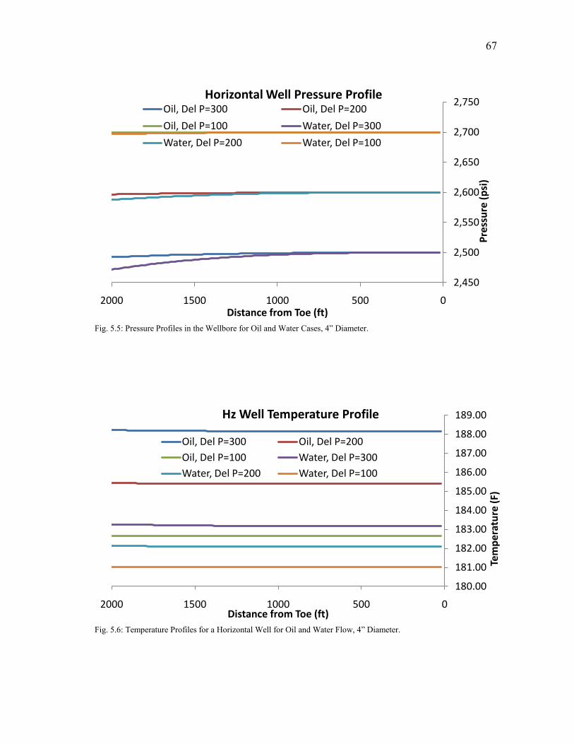
67

Fig. 5.5: Pressure Profiles in the Wellbore for Oil and Water Cases, 4” Diameter.

Fig. 5.6: Temperature Profiles for a Horizontal Well for Oil and Water Flow, 4” Diameter.

2,450

2,500

2,550

2,600

2,650

2,700

2,750

0500100015002000

Pre

ssu

re (

psi

)

Distance from Toe (ft)

Horizontal Well Pressure ProfileOil, Del P=300 Oil, Del P=200

Oil, Del P=100 Water, Del P=300

Water, Del P=200 Water, Del P=100

180.00

181.00

182.00

183.00

184.00

185.00

186.00

187.00

188.00

189.00

0500100015002000

Tem

per

atu

re (

F)

Distance from Toe (ft)

Hz Well Temperature Profile

Oil, Del P=300 Oil, Del P=200

Oil, Del P=100 Water, Del P=300

Water, Del P=200 Water, Del P=100

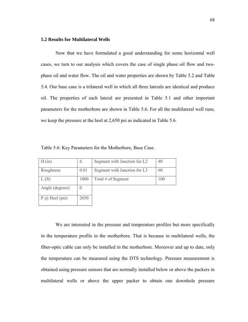
68

5.2 Results for Multilateral Wells

Now that we have formulated a good understanding for some horizontal well

cases, we turn to our analysis which covers the case of single phase oil flow and two-

phase oil and water flow. The oil and water properties are shown by Table 5.2 and Table

5.4. Our base case is a trilateral well in which all three laterals are identical and produce

oil. The properties of each lateral are presented in Table 5.1 and other important

parameters for the motherbore are shown in Table 5.6. For all the multilateral well runs,

we keep the pressure at the heel at 2,650 psi as indicated in Table 5.6.

Table 5.6: Key Parameters for the Motherbore, Base Case.

D (in) 6 Segment with Junction for L2 40

Roughness 0.01 Segment with Junction for L3 60

L (ft) 1000 Total # of Segment 100

Angle (degrees) 0

P @ Heel (psi) 2650

We are interested in the pressure and temperature profiles but more specifically

in the temperature profile in the motherbore. That is because in multilateral wells, the

fiber-optic cable can only be installed in the motherbore. Moreover and up to date, only

the temperature can be measured using the DTS technology. Pressure measurement is

obtained using pressure sensors that are normally installed below or above the packers in

multilateral wells or above the upper packer to obtain one downhole pressure

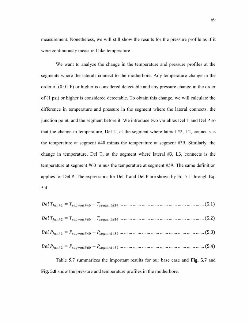
69

measurement. Nonetheless, we will still show the results for the pressure profile as if it

were continuously measured like temperature.

We want to analyze the change in the temperature and pressure profiles at the

segments where the laterals connect to the motherbore. Any temperature change in the

order of (0.01 F) or higher is considered detectable and any pressure change in the order

of (1 psi) or higher is considered detectable. To obtain this change, we will calculate the

difference in temperature and pressure in the segment where the lateral connects, the

junction point, and the segment before it. We introduce two variables Del T and Del P so

that the change in temperature, Del T, at the segment where lateral #2, L2, connects is

the temperature at segment #40 minus the temperature at segment #39. Similarly, the

change in temperature, Del T, at the segment where lateral #3, L3, connects is the

temperature at segment #60 minus the temperature at segment #59. The same definition

applies for Del P. The expressions for Del T and Del P are shown by Eq. 5.1 through Eq.

5.4

Table 5.7 summarizes the important results for our base case and Fig. 5.7 and

Fig. 5.8 show the pressure and temperature profiles in the motherbore.

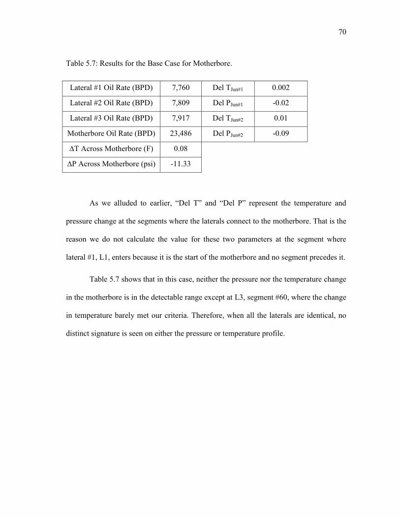
70

Table 5.7: Results for the Base Case for Motherbore.

Lateral #1 Oil Rate (BPD) 7,760 Del TJun#1 0.002

Lateral #2 Oil Rate (BPD) 7,809 Del PJun#1 -0.02

Lateral #3 Oil Rate (BPD) 7,917 Del TJun#2 0.01

Motherbore Oil Rate (BPD) 23,486 Del PJun#2 -0.09

∆T Across Motherbore (F) 0.08

∆P Across Motherbore (psi) -11.33

As we alluded to earlier, “Del T” and “Del P” represent the temperature and

pressure change at the segments where the laterals connect to the motherbore. That is the

reason we do not calculate the value for these two parameters at the segment where

lateral #1, L1, enters because it is the start of the motherbore and no segment precedes it.

Table 5.7 shows that in this case, neither the pressure nor the temperature change

in the motherbore is in the detectable range except at L3, segment #60, where the change

in temperature barely met our criteria. Therefore, when all the laterals are identical, no

distinct signature is seen on either the pressure or temperature profile.

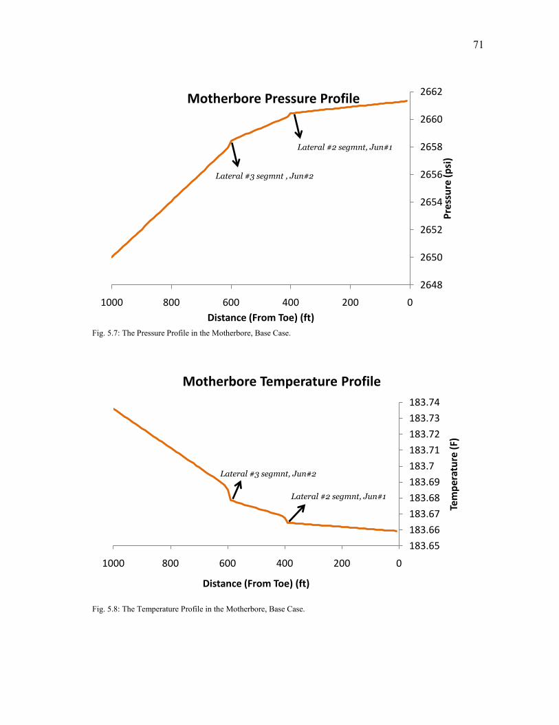
71

Fig. 5.7: The Pressure Profile in the Motherbore, Base Case.

Fig. 5.8: The Temperature Profile in the Motherbore, Base Case.

2648

2650

2652

2654

2656

2658

2660

2662

02004006008001000

Pre

ssu

re (

psi

)

Distance (From Toe) (ft)

Motherbore Pressure Profile

Lateral #3 segmnt , Jun#2

Lateral #2 segmnt, Jun#1

183.65

183.66

183.67

183.68

183.69

183.7

183.71

183.72

183.73

183.74

02004006008001000

Tem

per

atu

re (

F)

Distance (From Toe) (ft)

Motherbore Temperature Profile

Lateral #3 segmnt, Jun#2

Lateral #2 segmnt, Jun#1

72

It is noteworthy to highlight the change of the slope of the pressure and

temperature profiles shown on Fig. 5.7 and Fig. 5.8. The points where the slope changes

correspond to junction segments or segments where laterals connect to the motherbore.

For the pressure profile plot, the slope increases which indicates that the pressure

gradient increases. That is caused by the fact that more fluid is entering at these junction

points increasing the mass and velocity in the system. This increase in mass and velocity

causes an increase in the pressure drop as more fluid enters the motherbore from the

lateral. The increase in pressure drop gradient after each junction point causes an

increase in the temperature gradient. Therefore, we see both the pressure and

temperature gradients increase after each junction point.

In field applications, the interest is normally to identify which lateral or laterals

are damaged or are producing water if water cut is detected on the surface. To

investigate these issues, we will study the effect of varying three different parameters on

the pressure and temperature profiles. Namely, we will vary the permeability, length and

the water cut produced in one of the laterals and study the effect on the pressure and

temperature profiles. In this work, unless otherwise indicated, we choose lateral #2, L2,

and to its permeability, length and produced water cut. Table 5.8 shows a description of

the different runs made that will be referred to in the following discussion.

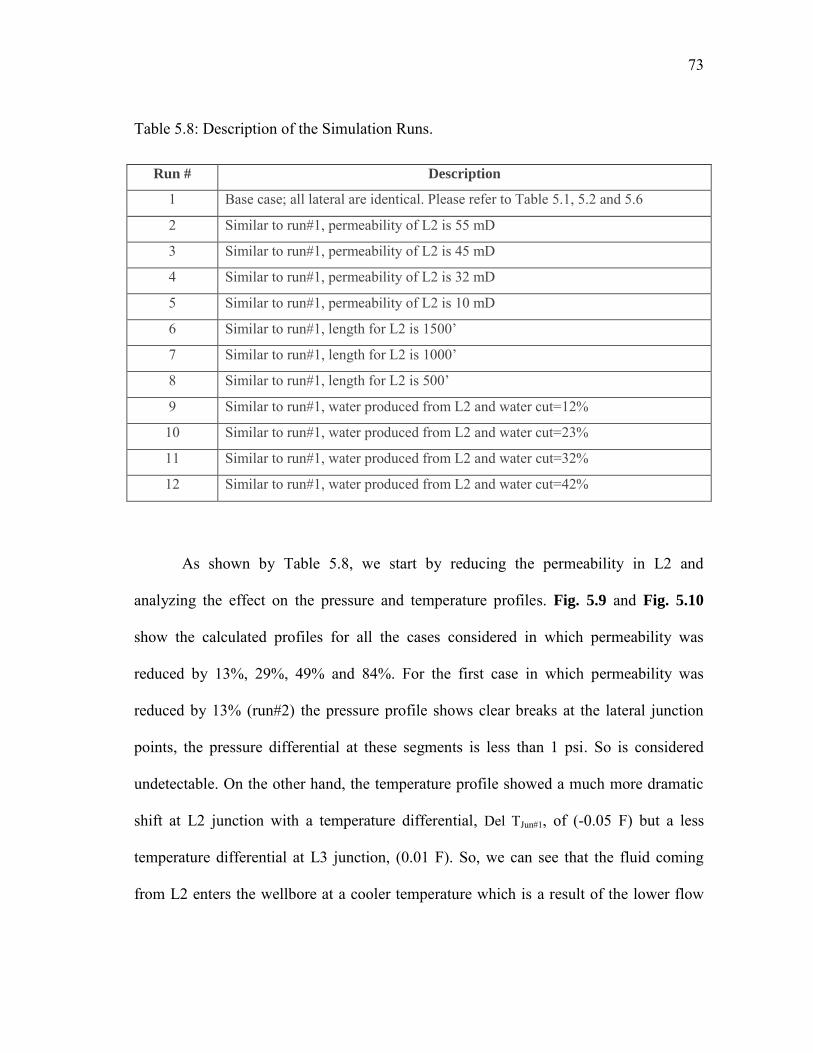
73

Table 5.8: Description of the Simulation Runs.

Run # Description

1 Base case; all lateral are identical. Please refer to Table 5.1, 5.2 and 5.6

2 Similar to run#1, permeability of L2 is 55 mD

3 Similar to run#1, permeability of L2 is 45 mD

4 Similar to run#1, permeability of L2 is 32 mD

5 Similar to run#1, permeability of L2 is 10 mD

6 Similar to run#1, length for L2 is 1500’

7 Similar to run#1, length for L2 is 1000’

8 Similar to run#1, length for L2 is 500’

9 Similar to run#1, water produced from L2 and water cut=12%

10 Similar to run#1, water produced from L2 and water cut=23%

11 Similar to run#1, water produced from L2 and water cut=32%

12 Similar to run#1, water produced from L2 and water cut=42%

As shown by Table 5.8, we start by reducing the permeability in L2 and

analyzing the effect on the pressure and temperature profiles. Fig. 5.9 and Fig. 5.10

show the calculated profiles for all the cases considered in which permeability was

reduced by 13%, 29%, 49% and 84%. For the first case in which permeability was

reduced by 13% (run#2) the pressure profile shows clear breaks at the lateral junction

points, the pressure differential at these segments is less than 1 psi. So is considered

undetectable. On the other hand, the temperature profile showed a much more dramatic

shift at L2 junction with a temperature differential, Del TJun#1, of (-0.05 F) but a less

temperature differential at L3 junction, (0.01 F). So, we can see that the fluid coming

from L2 enters the wellbore at a cooler temperature which is a result of the lower flow

74

rates produced from the lateral. L2 produced around 1700 – 1800 BPD less than the

other two laterals which translated into a lower temperature. Based on this finding, we

expect the temperature differential to increase as we reduce the permeability in L2

further.

In run#3, the permeability in L2 is reduced 29% and the pressure change at

segments #40 and #60 was less than 1 psi and so is undetectable. However, the

temperature profile shows a sharp jump at the junction of L2 with a temperature change,

Del TJun#1, of -0.1 F and a temperature change at the junction of L3 equal 0.02 F. The rate

produced from L2 is less in this run than was in run#2 resulting in a lower fluid

temperature for the fluid coming from L2. This shows up as a sharp jump in the

temperature profile at L2 junction. Also in this run, a better temperature change is

observed at the junction of L3. That is because the fluid in motherbore is cooled down

by the fluid from L2 more in this run compared to the previous run.

The same trend continues in run#4 and run#5. Fig. 5.10 shows clearly that as the

permeability is reduced further in L2, less fluid is produced, resulting in a less heating

effect. As the cooler fluid from L2 enters the motherbore, a higher temperature change is

observed at both junction points for both lateral #2 and lateral #3. Also, we can see that

the temperature change or differential is always higher at junction of L2 than it is at the

junction of L3. Table 5.9 summarizes the results for simulation runs in which

permeability of L2 was varied.

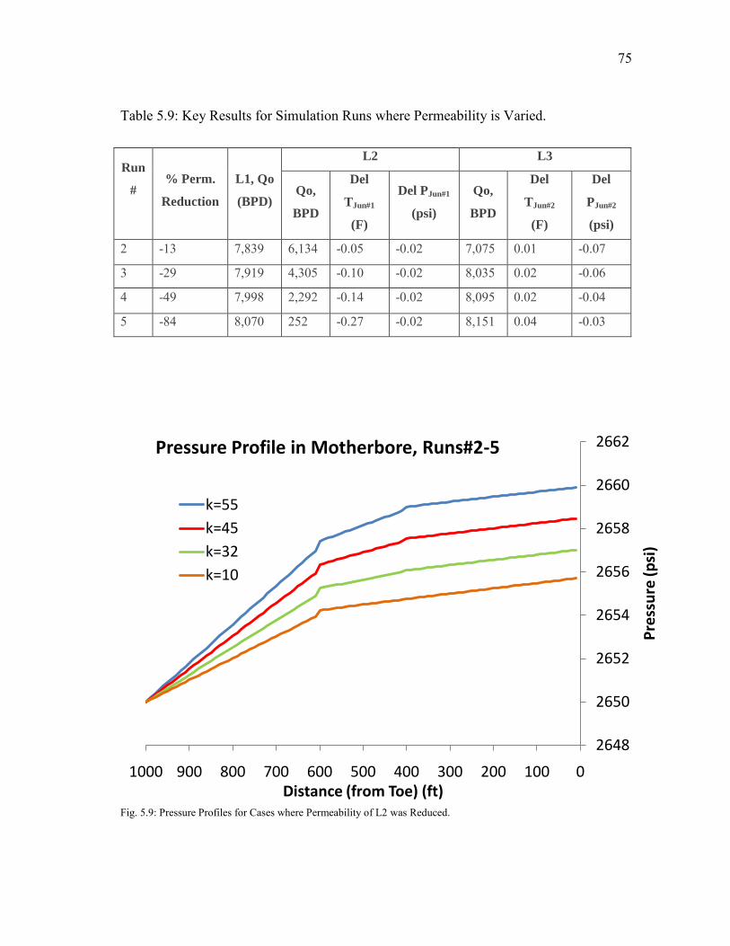
75

Table 5.9: Key Results for Simulation Runs where Permeability is Varied.

Run

#

% Perm.

Reduction

L1, Qo

(BPD)

L2 L3

Qo,

BPD

Del

TJun#1

(F)

Del PJun#1

(psi)

Qo,

BPD

Del

TJun#2

(F)

Del

PJun#2

(psi)

2 -13 7,839 6,134 -0.05 -0.02 7,075 0.01 -0.07

3 -29 7,919 4,305 -0.10 -0.02 8,035 0.02 -0.06

4 -49 7,998 2,292 -0.14 -0.02 8,095 0.02 -0.04

5 -84 8,070 252 -0.27 -0.02 8,151 0.04 -0.03

Fig. 5.9: Pressure Profiles for Cases where Permeability of L2 was Reduced.

2648

2650

2652

2654

2656

2658

2660

2662

01002003004005006007008009001000

Pre

ssu

re (p

si)

Distance (from Toe) (ft)

Pressure Profile in Motherbore, Runs#2-5

k=55

k=45

k=32

k=10

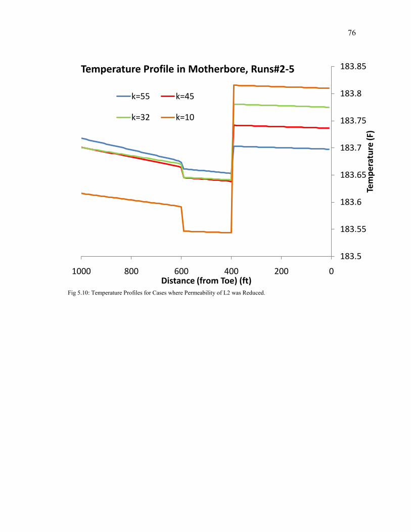
76

Fig 5.10: Temperature Profiles for Cases where Permeability of L2 was Reduced.

183.5

183.55

183.6

183.65

183.7

183.75

183.8

183.85

02004006008001000

Tem

pe

ratu

re (F

)

Distance (from Toe) (ft)

Temperature Profile in Motherbore, Runs#2-5

k=55 k=45

k=32 k=10

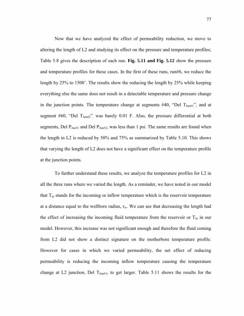
77

Now that we have analyzed the effect of permeability reduction, we move to

altering the length of L2 and studying its effect on the pressure and temperature profiles;

Table 5.8 gives the description of each run. Fig. 5.11 and Fig. 5.12 show the pressure

and temperature profiles for these cases. In the first of these runs, run#6, we reduce the

length by 25% to 1500’. The results show the reducing the length by 25% while keeping

everything else the same does not result in a detectable temperature and pressure change

in the junction points. The temperature change at segments #40, “Del TJun#1”, and at

segment #60, “Del TJun#2”, was barely 0.01 F. Also, the pressure differential at both

segments, Del PJun#1 and Del PJun#2, was less than 1 psi. The same results are found when

the length in L2 is reduced by 50% and 75% as summarized by Table 5.10. This shows

that varying the length of L2 does not have a significant effect on the temperature profile

at the junction points.

To further understand these results, we analyze the temperature profiles for L2 in

all the three runs where we varied the length. As a reminder, we have noted in our model

that Tin stands for the incoming or inflow temperature which is the reservoir temperature

at a distance equal to the wellbore radius, rw. We can see that decreasing the length had

the effect of increasing the incoming fluid temperature from the reservoir or Tin in our

model. However, this increase was not significant enough and therefore the fluid coming

from L2 did not show a distinct signature on the motherbore temperature profile.

However for cases in which we varied permeability, the net effect of reducing

permeability is reducing the incoming inflow temperature causing the temperature

change at L2 junction, Del TJun#1, to get larger. Table 5.11 shows the results for the

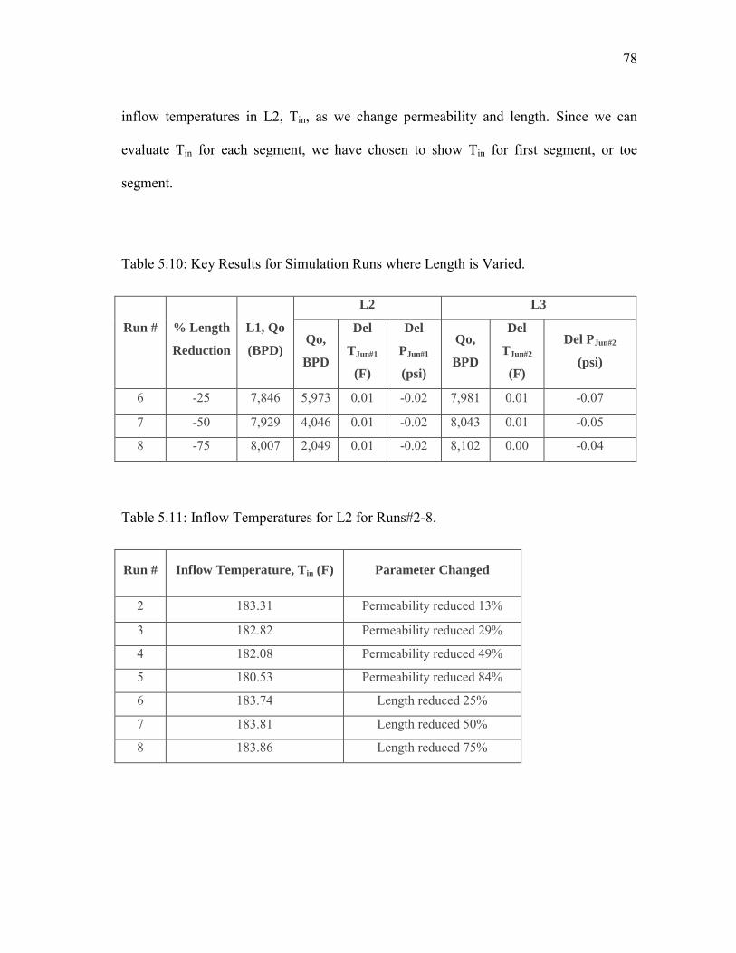
78

inflow temperatures in L2, Tin, as we change permeability and length. Since we can

evaluate Tin for each segment, we have chosen to show Tin for first segment, or toe

segment.

Table 5.10: Key Results for Simulation Runs where Length is Varied.

Run #

% Length

Reduction

L1, Qo

(BPD)

L2 L3

Qo,

BPD

Del

TJun#1

(F)

Del

PJun#1

(psi)

Qo,

BPD

Del

TJun#2

(F)

Del PJun#2

(psi)

6 -25 7,846 5,973 0.01 -0.02 7,981 0.01 -0.07

7 -50 7,929 4,046 0.01 -0.02 8,043 0.01 -0.05

8 -75 8,007 2,049 0.01 -0.02 8,102 0.00 -0.04

Table 5.11: Inflow Temperatures for L2 for Runs#2-8.

Run # Inflow Temperature, Tin (F) Parameter Changed

2 183.31 Permeability reduced 13%

3 182.82 Permeability reduced 29%

4 182.08 Permeability reduced 49%

5 180.53 Permeability reduced 84%

6 183.74 Length reduced 25%

7 183.81 Length reduced 50%

8 183.86 Length reduced 75%

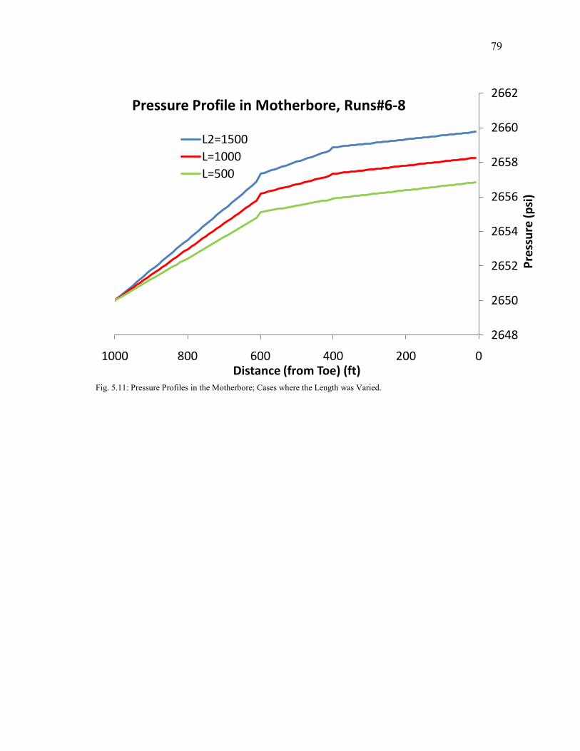
79

Fig. 5.11: Pressure Profiles in the Motherbore; Cases where the Length was Varied.

2648

2650

2652

2654

2656

2658

2660

2662

02004006008001000

Pre

ssu

re (p

si)

Distance (from Toe) (ft)

Pressure Profile in Motherbore, Runs#6-8

L2=1500

L=1000

L=500

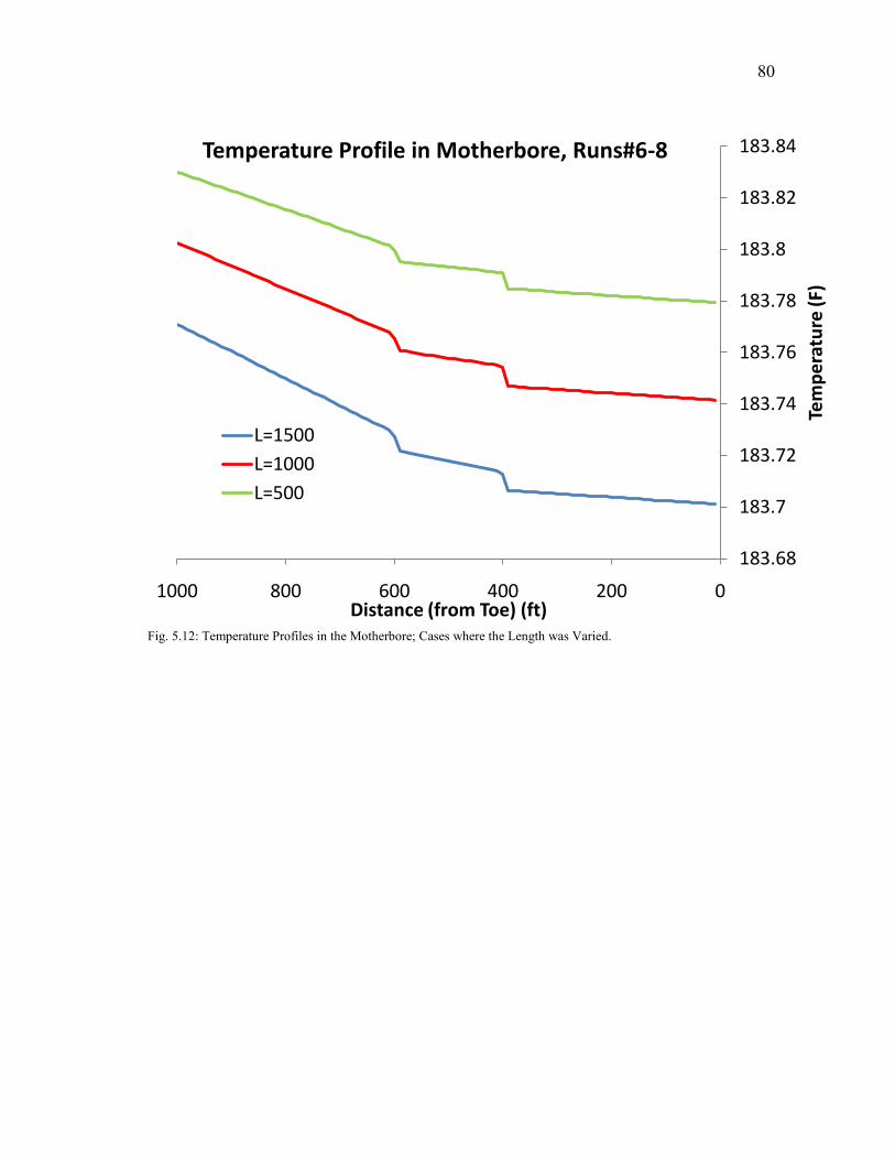
80

Fig. 5.12: Temperature Profiles in the Motherbore; Cases where the Length was Varied.

183.68

183.7

183.72

183.74

183.76

183.78

183.8

183.82

183.84

02004006008001000

Tem

pe

ratu

re (F

)

Distance (from Toe) (ft)

Temperature Profile in Motherbore, Runs#6-8

L=1500

L=1000

L=500

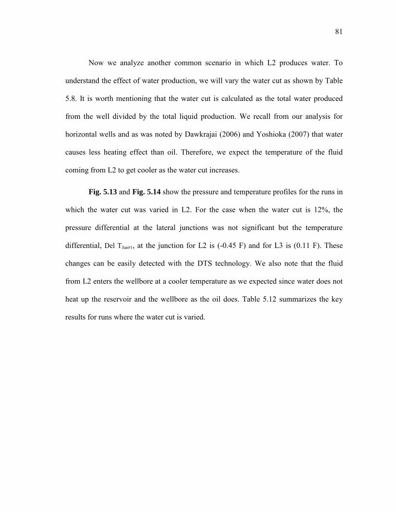
81

Now we analyze another common scenario in which L2 produces water. To

understand the effect of water production, we will vary the water cut as shown by Table

5.8. It is worth mentioning that the water cut is calculated as the total water produced

from the well divided by the total liquid production. We recall from our analysis for

horizontal wells and as was noted by Dawkrajai (2006) and Yoshioka (2007) that water

causes less heating effect than oil. Therefore, we expect the temperature of the fluid

coming from L2 to get cooler as the water cut increases.

Fig. 5.13 and Fig. 5.14 show the pressure and temperature profiles for the runs in

which the water cut was varied in L2. For the case when the water cut is 12%, the

pressure differential at the lateral junctions was not significant but the temperature

differential, Del TJun#1, at the junction for L2 is (-0.45 F) and for L3 is (0.11 F). These

changes can be easily detected with the DTS technology. We also note that the fluid

from L2 enters the wellbore at a cooler temperature as we expected since water does not

heat up the reservoir and the wellbore as the oil does. Table 5.12 summarizes the key

results for runs where the water cut is varied.

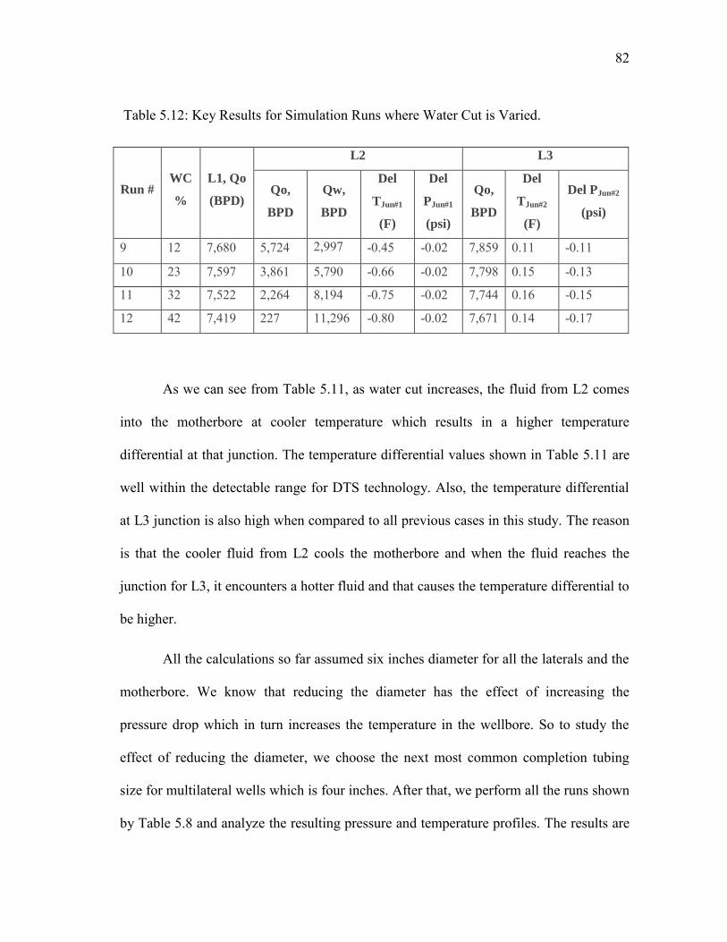
82

Table 5.12: Key Results for Simulation Runs where Water Cut is Varied.

Run # WC

%

L1, Qo

(BPD)

L2 L3

Qo,

BPD

Qw,

BPD

Del

TJun#1

(F)

Del

PJun#1

(psi)

Qo,

BPD

Del

TJun#2

(F)

Del PJun#2

(psi)

9 12 7,680 5,724 2,997 -0.45 -0.02 7,859 0.11 -0.11

10 23 7,597 3,861 5,790 -0.66 -0.02 7,798 0.15 -0.13

11 32 7,522 2,264 8,194 -0.75 -0.02 7,744 0.16 -0.15

12 42 7,419 227 11,296 -0.80 -0.02 7,671 0.14 -0.17

As we can see from Table 5.11, as water cut increases, the fluid from L2 comes

into the motherbore at cooler temperature which results in a higher temperature

differential at that junction. The temperature differential values shown in Table 5.11 are

well within the detectable range for DTS technology. Also, the temperature differential

at L3 junction is also high when compared to all previous cases in this study. The reason

is that the cooler fluid from L2 cools the motherbore and when the fluid reaches the

junction for L3, it encounters a hotter fluid and that causes the temperature differential to

be higher.

All the calculations so far assumed six inches diameter for all the laterals and the

motherbore. We know that reducing the diameter has the effect of increasing the

pressure drop which in turn increases the temperature in the wellbore. So to study the

effect of reducing the diameter, we choose the next most common completion tubing

size for multilateral wells which is four inches. After that, we perform all the runs shown

by Table 5.8 and analyze the resulting pressure and temperature profiles. The results are

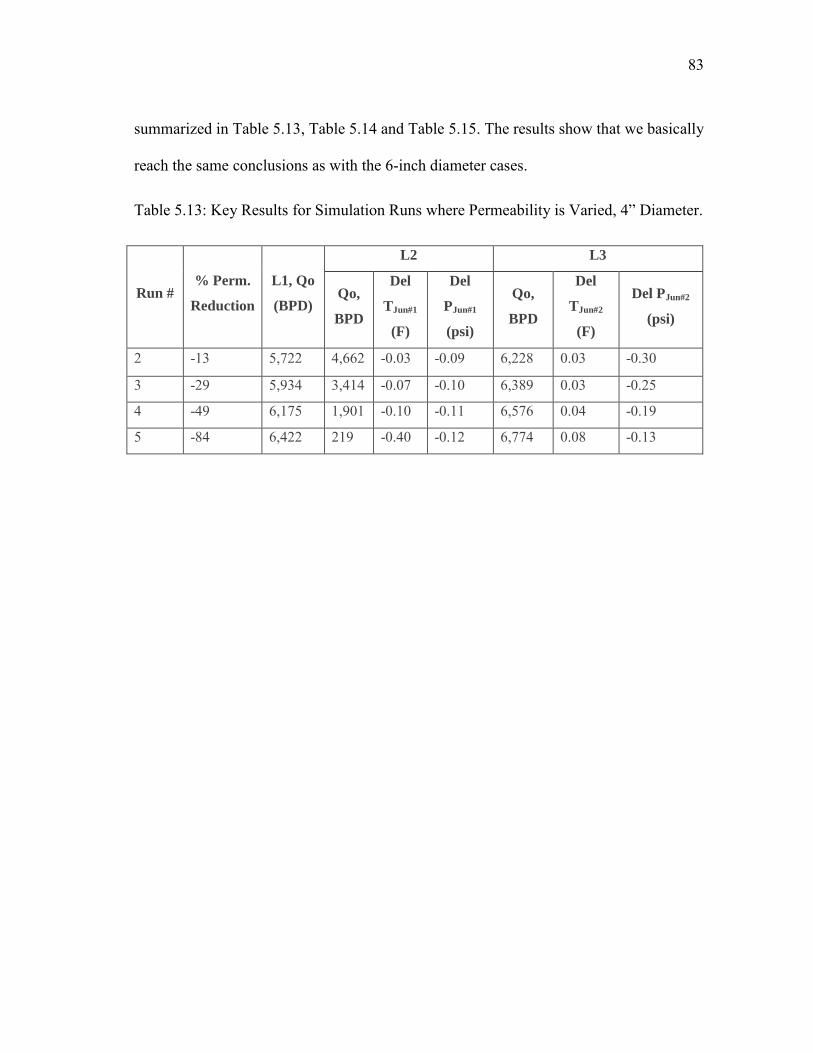
83

summarized in Table 5.13, Table 5.14 and Table 5.15. The results show that we basically

reach the same conclusions as with the 6-inch diameter cases.

Table 5.13: Key Results for Simulation Runs where Permeability is Varied, 4” Diameter.

Run # % Perm.

Reduction

L1, Qo

(BPD)

L2 L3

Qo,

BPD

Del

TJun#1

(F)

Del

PJun#1

(psi)

Qo,

BPD

Del

TJun#2

(F)

Del PJun#2

(psi)

2 -13 5,722 4,662 -0.03 -0.09 6,228 0.03 -0.30

3 -29 5,934 3,414 -0.07 -0.10 6,389 0.03 -0.25

4 -49 6,175 1,901 -0.10 -0.11 6,576 0.04 -0.19

5 -84 6,422 219 -0.40 -0.12 6,774 0.08 -0.13

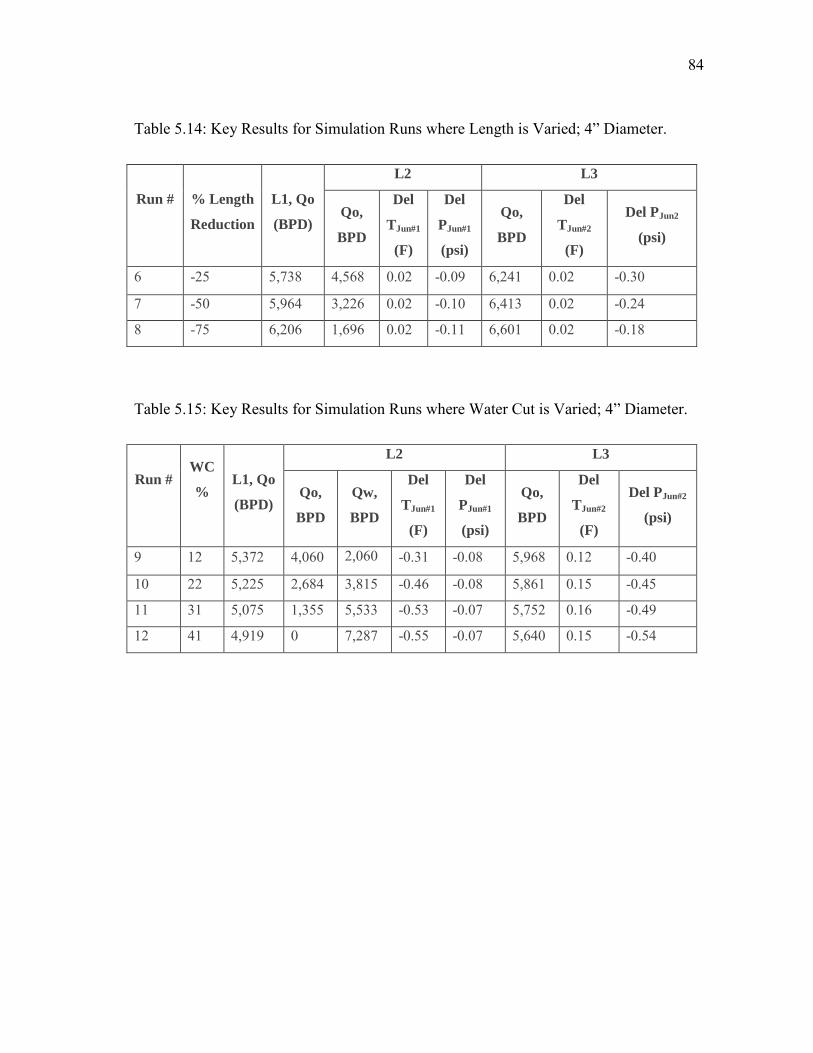
84

Table 5.14: Key Results for Simulation Runs where Length is Varied; 4” Diameter.

Run #

% Length

Reduction

L1, Qo

(BPD)

L2 L3

Qo,

BPD

Del

TJun#1

(F)

Del

PJun#1

(psi)

Qo,

BPD

Del

TJun#2

(F)

Del PJun2

(psi)

6 -25 5,738 4,568 0.02 -0.09 6,241 0.02 -0.30

7 -50 5,964 3,226 0.02 -0.10 6,413 0.02 -0.24

8 -75 6,206 1,696 0.02 -0.11 6,601 0.02 -0.18

Table 5.15: Key Results for Simulation Runs where Water Cut is Varied; 4” Diameter.

Run #

WC

%

L1, Qo

(BPD)

L2 L3

Qo,

BPD

Qw,

BPD

Del

TJun#1

(F)

Del

PJun#1

(psi)

Qo,

BPD

Del

TJun#2

(F)

Del PJun#2

(psi)

9 12 5,372 4,060 2,060 -0.31 -0.08 5,968 0.12 -0.40

10 22 5,225 2,684 3,815 -0.46 -0.08 5,861 0.15 -0.45

11 31 5,075 1,355 5,533 -0.53 -0.07 5,752 0.16 -0.49

12 41 4,919 0 7,287 -0.55 -0.07 5,640 0.15 -0.54

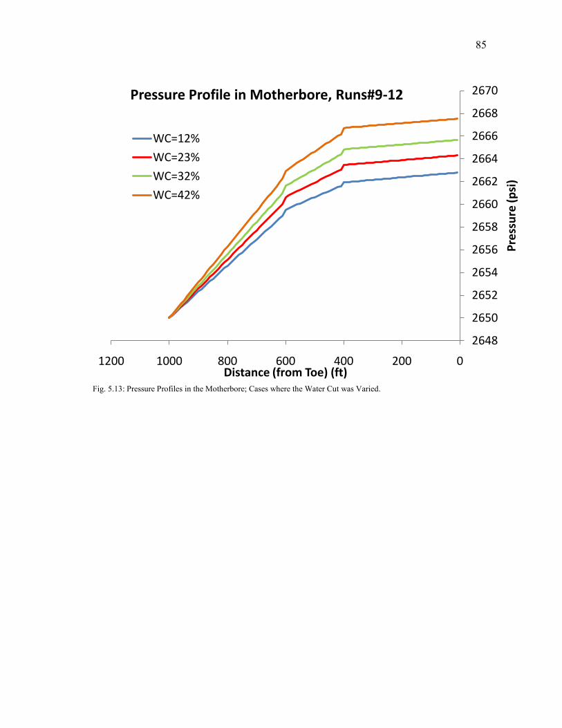
85

Fig. 5.13: Pressure Profiles in the Motherbore; Cases where the Water Cut was Varied.

2648

2650

2652

2654

2656

2658

2660

2662

2664

2666

2668

2670

020040060080010001200

Pre

ssu

re (p

si)

Distance (from Toe) (ft)

Pressure Profile in Motherbore, Runs#9-12

WC=12%

WC=23%

WC=32%

WC=42%

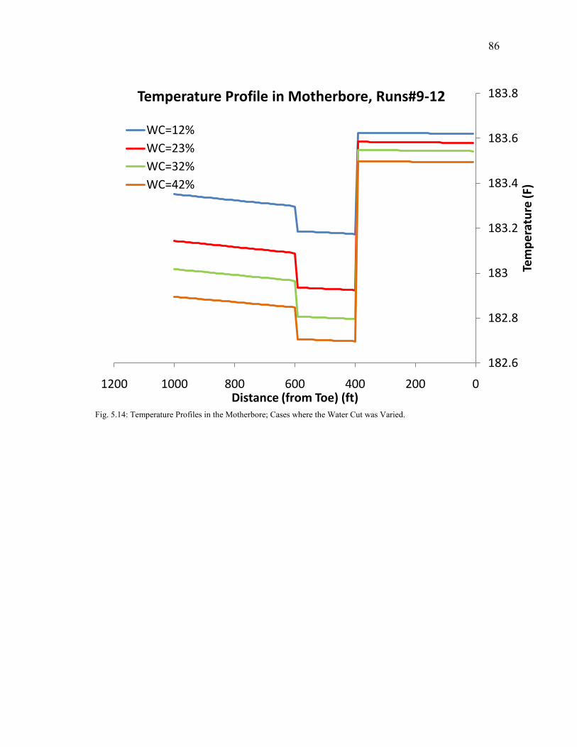
86

Fig. 5.14: Temperature Profiles in the Motherbore; Cases where the Water Cut was Varied.

182.6

182.8

183

183.2

183.4

183.6

183.8

020040060080010001200

Tem

pe

ratu

re (

F)

Distance (from Toe) (ft)

Temperature Profile in Motherbore, Runs#9-12

WC=12%

WC=23%

WC=32%

WC=42%

87

6. CONCLUSIONS AND RECOMMENDATIONS

6.1 Conclusions

In this research, we developed a steady-state model to calculate the pressure and

temperature profiles in multilateral wells. Drainage areas for all laterals were supplied as

input and the only interference between the laterals happens at the junction points in the

motherbore. Rock and fluid properties were calculated at average pressure and

temperature expected for each simulation run and then were kept constant throughout the

simulation run. This assumption is believed to be valid since the temperature and

pressure variations are not going to be significant to alter the fluid properties. The model

accounted for the pressure drop and the associated temperature change across the inflow

control valve, ICV. The pressure drop calculations across the valve were performed

using correlations provided by the equipment vendor.

In field applications, the interest is in identifying damaged lateral, the

contribution from each lateral or to identify which lateral or laterals are producing water

if water is seen on the surface. Therefore to investigate these issues, we varied the

permeability, length and water cut in lateral #2, or L2 in our notation, and studied the

effect on both the pressure and temperature profiles in the motherbore.

Our results show that reducing the permeability in L2 causes the fluid coming

from that lateral to be cooler than the fluid in the motherbore and resulted in a detectable

impact on the motherbore temperature profile that can be measured with DTS

technology. Also, introducing water in the L2 causes the fluid coming from L2 to be

88

cooler than the fluid in the motherbore and results in a detectable impact on the

temperature profile. On the other hand, reducing the length of L2 does not alter the

temperature profile in the motherbore significantly and change cannot be detected with

DTS technology. Moreover, the pressure profile in all cases does not show a detectable

change at the junction segments which indicates that the pressure data cannot be used to

identify damaged laterals or laterals which produce water, if present. The same

conclusions are reached whether we use 6-inch or 4-inch diameter wellbores.

6.2 Recommendations

Due to the time limitation, an inversion model was not developed and

verification of the model using field data was not possible in this research. Therefore, we

recommend developing an inversion model and testing it using field data to establish

applicability as well as limitation. Moreover, the reservoir model used assumed constant

rock properties and single phase flow in each reservoir segment. Although different

segments in the reservoir are allowed to have different permeabilities and different

phases, it is better to develop a numerical reservoir model that would relax a lot of the

assumptions made in this research. Also, such a model will enable analyzing cases where

the water produced either comes from the bottom formations or comes from the injection

wells. Moreover, the numerical model will allow interference between the laterals in the

reservoir which resembles the reality of multilateral wells.

89

REFERENCES

Al-Kaabi, A.O. 2008. Haradh-III: Industry’s largest Field Development with

Maximum Reservoir Contact Wells, Smart-Well Completions and the Ifield Concept.

SPE Production & Operations 23 (4): 444-447.

Bird, R. B., Stewart, W. E. and Lightfoot, E. N. 2002. Transport Phenomena.

New York: J. Wily.

Dawkrajai, P. 2006. Temperature Prediction Model for a Producing Horizontal

Well. PhD dissertation, University of Texas, Austin, TX.

Furui, K. 2003. A Rigorous Formation Damage Skin Factor and Reservoir Inflow

Model for a Horizontal Well. SPE Production & Facilities 18 (3): 151-157.

Glasbergen, G., Gualtieri, D., Domelen, M. S., Sierra, J. 2009. Real-Time Fluid

Distribution Determination in Matrix Treatments Using DTS. SPE Production &

Operations 24 (1): 135-146. SPE-107775-PA. DOI: 10.2118/107775-PA

Hembling, D.E., Berberian, G., Carter N. and John, N.G.2008. Enabling Efficient

Permanent Production Monitoring of Advanced Well Completions in Saudi Arabia

Using Fiber-optic Distributed Temperature Sensing. Paper SPE 115255 presented at the

SPE annual Technical Conference and Exhibition, Denver, CO, 21-24 September.

DOI:10.2118/115255-MS

Hill, A.D. 1990. Production logging: Theoretical and Interpretive Elements.

Monograph Series, SPE, Richardson, TX 14.

90

Jayawardena, S.S., Alkaya, B., Redus, C.L. and Brill, J.P. 2000. A New Model

for Dispersed Multi-Layer Oil-Water Flow. 2nd North American Conference on

Multiphase Technology, Banff, Canada, 40: 77-89.

Kim, D. and Ghajar, A.J. 2002. Heat Transfer Measurements and Correlations for

Air-Water Flow of Different Flow Patterns in a Horizontal Pipe. Experimental Thermal

and Fluid Science 25 (8): 659-676.

Mccain, W.D. 1990. The Properties of Petroleum Fluids. Tulsa, OK: PennWell

Books.

Nath, D.K., Finley, D.B., and Kaura, J.D. 2006. Real-Time Fiber-Optic

Distributed Temperature Sensing (DTS): New Applications in the Oilfield. Paper SPE-

103069 presented at the SPE Annual Technical Conference and Exhibition, San Antonio,

TX, 24-27 September. DOI: 10.2118/103069-MS.

Ouyang, L.B, 1998. Single-Phase and Multiphase Fluid Flow in Horizontal

Wells. PhD dissertation, Stanford University, Stanford, CA.

Prats, M. 1982. Thermal Recovery. Monograph Series, SPE, Richardson, TX 7.

Eclipse Technical Manual. 2008. Schlumberger. Houston, TX.

Sensornet Ltd. 2009. http://www.sensornet.co.uk/products-services/upstream-oil-

gas/digital-flow-profiling/.

91

Shi, H., Holmes, J., Durlofsky, L., Aziz, K., Daiz, L., Alkaya, B. and Oddie, G.

2005. Drift-flux Modeling of Two-Phase Flow in Wellbores. SPE Journal 10 (1): 24-33.

SPE-84228-PA. DOI:10.2118/84228-PA.

Shoham, O. 2006. Mechanistic Modeling of Gas-Liquid Two-Phase flow in

Pipes. Textbook Series, SPE, Richardson, TX.

Sieder, E.N. 1936. Heat Transfer and Pressure Drop of Liquids in Tubes.

Industrial and Engineering Chemistry 28: 1429-1435.

Sui, W. 2009. Determining Multilayer Formation Properties from Transient

Temperature and Pressure Measurements. PhD dissertation, Texas A&M University,

College Station, TX.

Yoshioka, K. 2007. Detection of Water or Gas Entry into Horizontal Wells by

Using Permanent Downhole Monitoring Systems. PhD dissertation, Texas A&M

University, College Station, TX.

92

VITA

Name: Rashad Madees K. Al-Zahrani

Address: Harold Vance Department of Petroleum Engineering

Texas A&M University

3116 TAMU – 507 Richardson Building

College Station, TX 77843-3116

Email Address Rashad.zahrani@aramco.com

rashadmalzahrani@gmail.com

Education: B.S., Petroleum Engineering, University of Kansas, 2005.

M.S., Petroleum Engineering, Texas A&M University, 2011