1 | P a g e

Utility-Integrated Biorefineries

Matt Byford and Andrew Robbins,

Luke Burton*, Jeffrey Fontenot* and Miguel Bagajewicz*

Department of Chemical, Biological and Materials Engineering

The University of Oklahoma

100 E. Boyd, Room T-335, Norman, OK 73019-0628

(*) Corresponding authors

2 | P a g e

Table of Contents

Introduction .................................................................................................................................................. 3

Background ................................................................................................................................................... 4

Centralized Utilities ....................................................................................................................................... 5

Value-Added Commodities ........................................................................................................................... 5

Capital Investment and Operating Costs ...................................................................................................... 8

Demand ......................................................................................................................................................... 9

Incentives ...................................................................................................................................................... 9

Algae ........................................................................................................................................................... 10

Mathematical Model .................................................................................................................................. 13

Results ......................................................................................................................................................... 23

Baseline Results ...................................................................................................................................... 23

Available Capital Investment .................................................................................................................. 24

Integrated Utilities .................................................................................................................................. 27

Algae Results ........................................................................................................................................... 28

Uncertainty Results ................................................................................................................................. 29

Further Study .............................................................................................................................................. 31

Conclusion ................................................................................................................................................... 32

Bibliography ................................................................................................................................................ 34

3 | P a g e

Introduction

The purpose of this report is to evaluate the feasibility and profitability of a proposed biorefinery.

A biorefinery is a chemical plant or cluster of plants that generates value-added products such as

biofuels and commodity chemicals from biomass. Biorefineries allow for the integration of

multiple processes that require the same biomass feed in one place in order to reduce the cost of

each individual process. This integration increases the economic viability of individual processes

by reducing operating, transportation, and utility costs. Production of commodity chemicals and

fuels from biomass is currently an emerging area of opportunity for several reasons. Small

commodity production from biomass is often more cost effective than current production

techniques. Since increased demand for biomass directly benefits farming, many government

benefits are available to companies investing in this area. The advantages of bio-technology in

the area of fuels production include decreased reliance on non-renewable resources such as fossil

fuels and decreased CO2 emissions. There is a high level of public interest in finding viable

biomass feedstocks. In recent years, the production of ethanol from corn has been highly

publicized. However, corn has several major problems. It generally requires high quality

farmland to produce, which could be used for other profitable crops. In addition, using corn to

produce fuel puts the fuel and food markets in direct competition, which has major social

consequences. In fact, the United Nations has claimed that U.S. subsidies on ethanol production

are partially responsible for the current global food crisis. Biorefining from cellulosic feedstocks,

specifically switchgrass, eliminates many of these problems. Cellulosic biomass grows naturally

in a wider range of climates than other feedstock options and the use of cellulosic biomass for

biorefining will not increase demand in other markets. Switchgrass has been shown to be the

4 | P a g e

premier cellulosic feedstock available by several published research studies and is considered the

best choice for a biorefinery.

The model used in this study optimizes the planning and development of a biorefinery in the

United States. The model takes into account the biorefinery location, raw materials locations,

transportation, market locations for products, demand and sales price of products, capital

investment, yearly operating costs, and centralized utilities. This model will be used to determine

the optimal grouping of commodities processes and biofuels production to maximize net present

value.

Background

Biofuels have the potential to reduce the United States’ dependence on fossil fuel resources

while stemming the tide of global warming. This study will investigate the necessary steps to

make biofuels production a reality. The first goal of this study is to determine whether or not the

production of biofuels is profitable on its own. Along with this, current government incentives

for production of biofuels will be investigated. Another goal of this study is to conclude whether

the grouping of biofuels production with commodity production will increase profitability. While

the profit generated by commodity production may be large enough to offset the deficit caused

by biofuels production, that alone is not enough to support the consolidation of the two

processes. The biofuels process must offer enough potential profit from government incentives,

decrease in capital, operating, and utility costs, and biofuels sales to support its incorporation in

the biorefinery. The final goal is to investigate the carbon emissions generated by the biorefinery

and strategies for reducing them. These are all important aspects of the problem that will be

addressed completely in this study.

5 | P a g e

Centralized Utilities The basic concept of centralized utilities is

recycling the utilities from one process

within the biorefinery to use them in

another process. Centralizing the utilities

used by multiple processes in a refinery

greatly decreases both the capital and

operating costs associated with utilities.

There are five major utilities that are taken

into account in the model: steam, cooling

water, electricity, air, and process water. Process water is water that directly contacts and mixes

with process components while cooling water and steam are used for heat exchange and never

directly contact process streams. Heat transfer between processes is modeled through the use of

steam and cooling water. When modeling the use of utilities in a biorefinery, both the cost of

each utility used based on the input stream and the operating and capital costs of operating

equipment associated with utilities such as water treatment plants, boilers, and cooling towers

were taken into account. In order to maximize the profitability of the biorefinery it is important

to minimize utility costs and utility integration is an effective way to do that.

Value-Added Commodities

There are a wide range of value-added chemicals that can be produced from biomass. The first

list of processes used in this study was based on previous study in the area of biorefining and

included fifty-eight processes. After developing a basic model, the number of processes was

reduced by removing any processes that were not profitable if operating cost and utility cost

6 | P a g e

were set equal to zero. This produced a list of seventeen processes that returned a positive net

present value under the zero costs condition. The second optimization model incorporated capital

investment, operating cost, and product demand. A few processes were eliminated on the basis

that the current demand is too low to support even the minimum capacity of a refinery setting.

The final screening included capital cost, operating cost, product demand, and utilility costs. The

results of this screening made up our base-case scenario. A flow diagram of the systematic

screening process and a diagram of the initial process list are included below.

•Capital Cost

•Operating Cost=0

•No Utilities

First Screening

• Capital Cost

• Add Operating Cost

• No Utilities

• Incorporate Demand and Capacity

Second Screening

•Capital Costs

•Operating Costs

•Add Utilities and Integration

Final

Screening

7 | P a g e

Switchgrass

Lignin Syngas

Methanol Biodiesel

Biogasoline

Biofuels

Glucose

Ethanol

Acetic Acid

Ethylene

Vinyl Acetate Monomer

Polyvinyl Acetate

Acetic Anhydride

Ethyl Lactate

Acetate

Lactic Acid

Dilactide

Acrylic Acid

2,3-Pentane-dione

Acetic Acid

Ethyl Acetate

Sodium

Succinate

SuccinicAcid

Butaniediol

Tetrahydro-furan

γ-butyrolactone

Malic Acid

L-Aspar

tic Acid

Fumaric Acid

L-Aspartic Acid

3-Hydroxy-

propionic Acid

Glutamic Acid

1,3-Propanediol

Glucaric Acid

Polyglucaric Acids

Lactones

Amides

Pyruvate

Acetate

Ethanol

Acetone

Butyrate

Butanol

Glucose

Sorbitol

Propylene Glycol

Lactic Acid

LevulinicAcid

Tetrahydrofuran

Succinic Acid

γ-butyrolactone

5-Hydroxymethyl-

fufural Furan dicarboxylicAcid

3-Hydroxybutyro-

lactoneFurans

Amino Acid

Analogs

Itatonic Acid

PolyitatonicAcid

Methyl Butanediol

8 | P a g e

Capital Investment and Operating Costs

To obtain Capital and Operating Costs for use in our mathematical model, an incremental model

was used. That is, it was assumed that where alpha and beta are

constants. To determine the value of alpha and beta, the processes were simulated in SuperPro at

varying capacities. The cost is then plotted against the capacity and a linear fit is obtained. The

figure above shows a sample of the plot generated.

This process was used to find analytical models for all of the processes included in our model.

Capital and Operating Costs constants for the utilities were calculated separately from overall

costs; the same basic method was used to determine alpha and beta coefficients for the capital

investment and operating costs associated with utilities. These estimations were based off the

major pieces of equipment associated with each utility. For example, the estimation of costs

associated with steam was based on the cost of a boiler plant.

y = 0.0001x + 427015Slope: 1x10-4 $/kg

Intercept: $427,015

0.00E+00

2.00E+06

4.00E+06

6.00E+06

8.00E+06

1.00E+07

1.20E+07

1.40E+07

0 5E+10 1E+11 1.5E+11

FCI $

kg/yr

FCI - Cooling Water

9 | P a g e

Demand

In the mathematical model, the value for demand determines how much of a product the model is

allowed to sell in kg/year. For example, if the demand value for biodiesel is 109, the model will

produce no more than 109 kg/year of biodiesel. Obviously, there is no easy or foolproof way to

know how much of each product can be sold. Instead, the values for demand were estimated

from known U.S. chemical consumptions (since the chemicals will be sold in the U.S.). These

values were found online; the specific websites can be found in the sources appendix in the

supporting data. In some cases, only world consumption was available. When data for chemicals

with known U.S. and world consumption was examined, it was found that U.S. consumption was

consistently around 25% of world consumption for chemical commodities. Given this, the U.S.

consumption was calculated for most of the chemicals in the model. However, the U.S.

consumption should not be used as the value for demand. To see this, imagine what would

happen if a new plant introduced supply of a commodity equal to that commodity’s annual

consumption. It is obvious that the market for the commodity would be destroyed. To account

for this, the demand values were chosen as 20% of U.S. consumption. This was thought to be a

production level which would not have a substantial negative impact on the market.

Sample Demand

Commodity Gasoline Biodiesel 3-Hydropropionic

Acid

Levulinic

Acid

Demand

(kg/yr) 77,400,000,000 27,600,000,000 655,000,000 205,000,000

Incentives

A major goal when manufacturing biofuels is maximizing the benefit obtained from government

subsidies. The first step in this direction is awareness of what incentives are available. The

Department of Energy maintains a comprehensive database of government subsidies in all areas

10 | P a g e

of renewable energy. For this project, the relevant incentives were identified and incorporated in

the mathematical model.

There are two main types of incentives available: tax credits and grants/loans. Tax credits are a

flat reduction in taxes. For example, if a $1/gallon tax credit is available of biodiesel and 100,000

gallons of biodiesel is manufactured at facility A, facility A can claim a $100,000 reduction in

their taxes for that year. Tax credits are especially prominent in modeling economic ventures

because, unlike grants/loans, they are guaranteed. This is extremely important in business where

low risk is valued highly. Grants and loans, on the other hand, are distributed by the applicable

government agency to projects which they feel are deserving. While this can be extremely

rewarding, it also carries the risk of not receiving the subsidy.

National Biofuels Incentives

Program Agency Type Amount Likelihood

VAPG USDA Grant 300,000 Possible

Rural Business-Cooperative

Service USDA Loan 250,000,000 Possible

B&I Guaranteed Loan Program USDA Loan 40,000,000 Possible

Cellulosic Biofuel Producer

Tax Credit Congress

Tax

Credit

$1.01/gallon

produced Guaranteed

Selected State Biofuels Incentives

Program State Type Amount Likelihood

Biodiesel Production Tax

Credit IN

Tax

Credit

$1/gal biodiesel up to $5

million Guaranteed

Biodiesel Production Tax

Credit KY

Tax

Credit

$1/gal biodiesel up to $5

million Guaranteed

Algae

In recent years, algae has rapidly gained attention as a potential feedstock for biofuels. The

technology necessary to produce biodiesel from triglycerides (such as algal oil) has been

11 | P a g e

available since the late 1930s. However, available sources of triglycerides (such as soybean oil)

have always required heavy consumption of farmland. Since that put them in direct competition

with food crops, the production of biodiesel from triglycerides has never been commercially

feasible. Algae could change all of that. Recent research suggests that algae could produce higher

yields of oil than conventional oil crops. In addition, algae can be cultivated in coastal waters,

thus eliminating the competition with food crops. Furthermore, in recent studies, algae has

demonstrated the ability to sequester up to 50% of CO2 from gas streams passed through the

algae. Clearly, algae has potential as a feedstock. It remains to be seen whether it can be a

profitable addition to a biorefinery.

Since the biorefinery will likely be built inland, only land-based algae cultivation methods were

considered. Aquatic cultivation is also viable, but coastal locations are likely not suitable for a

biorefinery given the large amounts of land-based feedstock required. In addition, both states

identified as optimal locations in terms of government biofuel incentives are landlocked. There

are three common approaches to land-based algae cultivation: open pools, closed pools, and

photobioreactors. Open pools are exactly what they sound like: open air pools filled with water

and seeded with algae. Closed pools are essentially open pools with greenhouses constructed

over the top. Photobioreactors are structures designed specifically for growing algae

productively. For a biorefinery application, open pools are the only viable choice. The other

options produce better yields and eliminate some of the problems associated with open pools, but

are impractical on a large scale.

The production of biodiesel from algal oil is performed by transesterification with methanol. The

algal oil is a triglyceride with molecular weight of approximately 930 g/mol. When methanol is

12 | P a g e

added to the oil, the methanol groups substitute into the triglyceride to produce glycerol and

three methyl esters with molecular weights of approximately 310 g/mol. This falls into the

molecular weight range of diesel (or biodiesel in this case). To catalyze the reaction, alkali

hydroxides or methoxides are used. The catalyst activates methanol by removing a proton from

the alcohol group. Sodium methoxide (NaOCH3) is considered the best catalyst from a

commercial point of view. The effluent from the reaction vessel is a mixture of glycerol,

biodiesel, and unreacted triglycerides. This stream is either centrifuged with water or extracted

with ether to separate the glycerol and the biodiesel. It is then desired to purify the biodiesel.

However, since the remaining triglycerides are in a basic state, they are soaps and act as

emulsifying agents. To achieve a good separation, the biodiesel stream is washed with water

which has been acidified to a pH of approximately 4. This returns the triglycerides to their

neutral configuration, which allows them to be extracted in the water stream. The biodiesel is

then dried to meet fuel standards.

To include algae in the mathematical model, it was necessary to compute each of the relevant

sets of coefficients: stoichiometric, utility consumption, utility generation, capital, and operating

costs. Stoichiometric coefficients were computed in two stages: one for algae production and one

for transesterification. Values for the amount of CO2 required for algae production was found in

recent research. Values for transesterification were easily computed from the chemical equation.

For the other four sets, a SuperPro simulation for the transesterification of soybean oil was

adapted for algal oil. The coefficients were then computed from the simulation results. The

methods used were identical to those used previously for other processes.

13 | P a g e

Mathematical Model

GAMS/CPLEX was used to optimize the select processes and design parameters within the

biorefinery to maximize the net present value.

Set Name

i,k Processes

j,jj Chemicals

t,tt Time Periods

m Market Locations

n Raw Material Locations

p Plant Locations

u Utilities

The objective function maximized the net present value (maxNPV). This function summed the

proceeds returned to the investors each year (Pt) and adjusted this value to the current time

period by using the interest rate. The capital investment (capinv) was then subtracted from this

sum.

(1)

Economic Equations

The cash on hand for each year is equal to the previous year’s cash plus the total revenue from

all processes minus the money returned to the investors all costs, including transportation costs,

operating costs, and fixed costs. In the first year, the capital investment is added to the cash.

(2)

The tax equation is equal to the tax rate times the cash flow, not including depreciation.

(3)

14 | P a g e

There is also a stipulation that the cash on hand for each year must be larger than a certain value

for contingencies. In this case, the contingency money is 1% of the capital investment.

(4)

The capital investment for this program is defined as the sum of the fixed costs and material

costs for all years adjusted to the current time period.

(5)

An additional constraint was added to ensure that the capital investment is less than the

maximum available investment, which was set in advance.

(6)

The fixed cost for each year is the sum of the initial fixed costs, expansion fixed costs, and

utilities fixed costs for all the processes or utilities.

(7)

The initial fixed capital investment for each process was modeled as a linear function with a

minimum cost to build the process (alphai) and an incremental cost (betai) associated with the

capacity of the process initially. isBuilti,t is a binary variable that is equal to 1 in the year the

process is built and is equal to 0 for all other years.

(8)

15 | P a g e

The expansion is similarly based on a minimum cost (alpha2i) and an incremental cost (beta2i).

The coefficients alpha2 and beta2 are 71% of alpha and beta, respectively. This percentage is

based on the price to expand a process with the infrastructure already built versus building a

grassroots plant. Similar to isBuilti,t, isExpandedi,t is also a binary variable, though it indicates

whether or not a process is expanded in the year indicated.

(9)

The fixed costs for the utilities closely resemble the cost equations for the chemical processes

above.

(10)

(11)

(12)

The total operating cost is equal to the sum of the operating costs for all processes and utilities.

(13)

The operating cost is based on a linear model, similar to the model for fixed costs.

(14)

(15)

16 | P a g e

The revenue for each chemical is the sum of all the chemicals sold to markets at the price that

can be obtained from that market.

(16)

The cost associated with the raw materials is equal to the sum of raw material bought at each

field times the raw material price for that location.

(17)

The transportation cost for any year is the sum of the cost of transporting raw materials from

their fields and the cost to move products to their markets.

(18)

The product and raw material transport costs are equal to the amount of material moved

multiplied by the distance traveled and the cost to move the material per kilogram per mile.

(19)

(20)

Constraints and Material Balances

These equations ensure that mass is not created or destroyed and that the model does not violate

common sense. Equation 21 ensures that any one process is only built once.

(21)

17 | P a g e

The following equation makes sure that the process cannot be expanded and built in the same

year.

(22)

The next equation sums the time periods, tt, up to the present year. Its purpose is to keep the

process from being expanded until it is built.

(23)

The utility building and expansion equations are essentially the same as those for the chemical

processes above.

(24)

(25)

(26)

The capacity for each process is equal to the initial capacity that year (the initial capacity is zero

in years the process is not built) plus the capacity from the year before plus any expansions that

occurred this year.

(25)

The following equation causes the process capacity to be larger than the sum of its products.

(26)

18 | P a g e

The initial capacity must be zero for all years except the one in which the process is built, and in

that year, the initial capacity must be larger than the minimum capacity.

(27)

Similarly, the initial capacity in the year the process is built must be less than the maximum

allowable capacity.

(28)

Similar equations exist for the process expansion term.

(29)

(30)

This equation allows for setting a maximum allowable number of expansions.

(31)

The utility capacity is the sum of the initial capacity for utilities, the capacity last year, and the

expansion for that year.

(32)

The makeup term will be explained later in the Utility Integration subsection. It is essentially the

amount utility that the process requires. This equation ensures that the utility capacity is equal to

or larger than the required utility.

(33)

19 | P a g e

These equations closely resemble Equations 27-31 above.

(34)

(35)

(36)

(37)

(38)

Qp is a binary variable which is set to 1 if the biorefinery is to be built at this location or zero if it

is not. This equation ensures that the biorefinery is only located at one optimal location.

(39)

The following equation makes sure that the amount of raw material purchased from any one field

does not exceed the maximum amount of raw material that field can produce.

(40)

The sum of the raw materials needed for all the processes must equal the amount of raw

materials purchased.

(41)

20 | P a g e

The input to any process is equal to the raw materials coming from other processes plus the

amount of raw materials purchased for this process from raw material producers.

(42)

The input into a process is defined as a fraction of the total input into that process. The value of

this fraction is fi,j for each process and chemical.

(43)

This is the primary mass balance which states that the sum of all the inputs into a process must

equal the sum of all the outputs from the process.

(44)

The output from the process must be greater than or equal to the minimum capacity of the

process, if the process has been built.

(45)

The flow of a chemical from this process to another cannot exceed the output of this chemical

from this process. Gamma is a binary parameter which is equal to one if the process can transfer

this chemical to another process and is equal to zero if the process cannot.

(46)

21 | P a g e

The output from a process is defined as a stoichiometric fraction of the total output from that

process. The fraction of the output for each chemical is gi,j.

(47)

The output of the process is equal to the amount to be sold plus the amount of product that is

transferred to use in other processes.

(48)

The amount of chemicals from all the processes to be sold is equal to the amount of chemicals

sold at markets from the plant.

(49)

The amount of chemical to be sold cannot exceed the demand for that chemical.

(50)

The amount of product sold to one market cannot exceed a predetermined limit per year.

(51)

The amount of product sold to one market cannot exceed a certain number for the sum of all

years the chemical is sold.

(52)

22 | P a g e

Intermediate Processes

Some of the processes considered do not use switchgrass as a raw material, but instead use a

chemical that must be processed from switchgrass as a feedstock. This equation is set up to

ensure that these secondary processes cannot be built unless the intermediate chemical is being

produced from another process in the biorefinery.

Prereqi,k is a binary parameter that is set to one if the process requires a feedstock other than

switchgrass and zero if the process uses switchgrass.

(53)

The following equation is only applicable if the process requires an intermediate feedstock. This

equation makes sure that the input to the secondary process does not exceed the amount of

chemical the process producing its feedstock can produce.

(54)

Utility Integration

The idea of utility integration allows for utilities being created in one process to be used in

another. If a process creates a utility, the utility generation variable is equal to a coefficient times

the total input into the process.

(55)

Similarly, the amount of utility consumed by a process is equal to a coefficient times the total

input into the process

(56)

23 | P a g e

The makeupu,t variable is the amount of utility that is required beyond what is created in all the

processes. If a process generates enough utility for all the processes that are built, then the

makeup is not needed and no fixed capital will be spent on creating that utility.

(57)

Results

Baseline Results

After narrowing the list of processes to be incorporated to thirteen, the final screening was run.

The major variables that were included in the model were the processes built (including

biofuels), the capacity of each process, the capacity of expansions, the location of the

biorefinery, the markets for buying and selling, and the possible utility schemes. As mentioned

before, the objective of the model was to maximize the net present value of the refinery. The

model was initially based on a

maximum capital investment of

$2.5 billion. The current available

government tax credit of $1 per

gallon of biofuel produced was

included by adding it directly to the sales price of the biofuels. For example, the original sales

price of biodiesel was set at $1.23 per kilogram but the sales price incorporated into the model

was $1.56 per kilogram after accounting for the $1 per gallon tax credit. The results of the

baseline (initial) optimization are organized in the included table.

With the current demands of each process and sales prices in the United States the profitable

processes to incorporate in the biorefinery are the production of biofuels, 3-hydroxypropionic

Baseline Results

Location: Processes: Capacity (kg/yr)

Lexington, KY Biofuels

3-HPA

Levulinic Acid

Tetrahydrofuran

1,440,000,000

6,500,000

57,600,000

40,000,000

TCI ($) NPV ($) ROI

176,000,000 687,000,000 24.5%

24 | P a g e

acid, levulinic acid, and tetrahydrofuran. The raw materials, specifically the switchgrass are

supplied from across the state of Kentucky. The biofuels are sold in Louisville, KY while the

chemical commodities are sold in various locations ranging from Missouri to Florida. Initially

only enough levulinic acid is produced to be used as the building block for tetrahydrofuran

production, but after the second year expansion levulinic acid is also sold.

The chemical commodities to be produced in the biorefinery have a variety of applications. 3-

hydroxypropionic acid, or 3-HPA is used as a building block for a variety of chemicals including

acrylics, malonic acid, 1,3-propanediol, EEP, and some polymers. Tetrahydrofuran, also known

as THF, is used primarily as a solvent for industrial resins. It is also used to coat PVC and

cellophane, and is used in paint manufacture while levulinic acid has a wide variety of uses from

the production of synthetic rubber and pharmaceuticals to cigarettes.

Therefore from the base-case results it can be concluded that the mathematical model supports

the hypothesis that the combination of multiple processes in a single biorefinery from a common

feedstock is an optimal investment. The results also support the inclusion of biofuel production

in a biorefinery setting as a profitable choice. The results from the initial model will be used in a

stochastic analysis which will determine the uncertainty of the results and find an optimal design

given uncertainty.

Available Capital Investment

After examining the base-scenario and the effect of uncertainty on the results it was important to

study the different profitable scenarios under varying ranges of available capital investment. For

this study the amount of available capital investment was ranged from $10 million to $2.5

billion. A graph of the results comparing available capital to net present value can be seen here.

25 | P a g e

From a maximum investment of

$10 million to $28.5 million it is

not profitable to build any single

or combination of processes. From

$28.5 million to $140 million the

optimal net present value corresponds to a tetrahydrofuran plant built in Lafayette, LA. Over the

range of $140 million to $176 million in available capital the highest net present value is found

by the building of a biofuels plant in Lexington, KY, the same location as the base-case scenario.

Finally from $176 million to $2.5 billion the highest net present value is associated with the

base-case scenario discussed earlier, a biorefinery including biofuels, 3-HPA, levulinic acid, and

tetrahydrofuran production in Lexington, KY. This is not to say that these three scenarios are the

only possibilities that yield a positive net present value just that they are the most profitable

decision when optimizing net present value, when considering the available capital. The next

analysis performed using the mathematical model was to compare the return on investment

(ROI) for a varying range of available capital investments. The same range of available capital

was used that was examined for the available capital investment versus net present value study. It

is important at this time to comment on the definition of return on investment that was used for

this study. There are varying definitions of ROI depending on their application and the focuses of

the study. The ROI equation used for this study is shown below.

0

200

400

600

800

0 50 100 150 200 250

NP

V in

Mill

ion

s ($

)

Available Capital Investment in Millions ($)

NPV v. Available Capital Investment

Base-case Scenario

capinvN

i

P

ROI tt

t

)1(

26 | P a g e

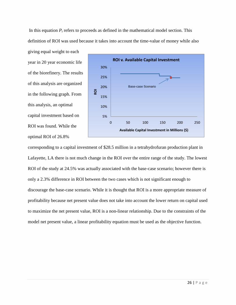
In this equation Pt refers to proceeds as defined in the mathematical model section. This

definition of ROI was used because it takes into account the time-value of money while also

giving equal weight to each

year in 20 year economic life

of the biorefinery. The results

of this analysis are organized

in the following graph. From

this analysis, an optimal

capital investment based on

ROI was found. While the

optimal ROI of 26.8%

corresponding to a capital investment of $28.5 million in a tetrahydrofuran production plant in

Lafayette, LA there is not much change in the ROI over the entire range of the study. The lowest

ROI of the study at 24.5% was actually associated with the base-case scenario; however there is

only a 2.3% difference in ROI between the two cases which is not significant enough to

discourage the base-case scenario. While it is thought that ROI is a more appropriate measure of

profitability because net present value does not take into account the lower return on capital used

to maximize the net present value, ROI is a non-linear relationship. Due to the constraints of the

model net present value, a linear profitability equation must be used as the objective function.

5%

10%

15%

20%

25%

30%

0 50 100 150 200 250

RO

I

Available Capital Investment in Millions ($)

ROI v. Available Capital Investment

Base-case Scenario

27 | P a g e

Integrated Utilities

The diagram below shows the integration of utilities in the base-case scenario.

Although the base-line scenario included integrated utilities, the same model was run excluding

integrated utilities to examine the difference. The difference between the two scenarios is two

fold. First non-integrated utilities does not allow for transfer of excess utilities from one process

to another or the recycling of utilities. At the same time individual utility infrastructures must be

built for each process as opposed to a single infrastructure for the refinery. The results of the

comparison are included in the table below.

Integrated Non-integrated

Net Present Value $687,000,000 $665,000,000

Capital Investment $176,000,000 $185,000,000

Return on Investment 24.5 % 22.9 %

28 | P a g e

From the economic comparison it is clear that integrated utilities increases the profitability of a

biorefinery. There is a 5.2% savings in capital investment when comparing the two scenarios.

More significantly, the inclusion of integrated utilities accounts for a $22 million increase in the

net present value of the biorefinery over the 20 year economic lifetime. While the integration of

utilities does not affect the overall feasibility of the biorefinery it does significantly improve

profitability as expected

Algae Results

To determine how the inclusion of algae would affect the results, the baseline scenario was run

again with algae included. The results were very similar, as shown in the table below; the same

processes were built with the same capacities as the run without the algae.

The major difference was that instead of emitting the CO2 produced by the processes; it was fed

to the algae first, resulting in a substantial decrease in emissions. Compared to the baseline

results, the algae results were economically comparable. The NPV was 642 million dollars, 6.6%

Results w/o Algae Results w/ Algae

Location Lexington, KY Lexington, KY

Processes Biofuel

3-HPA

Levulinic Acid

Tetrahydrofuran

Biofuel

3-HPA

Levulinic Acid

Tetrahydrofuran

Algae

Capacities (kg/yr) 1,440,000,000 (Biofuel)

6,500,000 (3-HPA)

57,600,000 (LA)

40,000,000 (THF)

1,440,000,000 (Biofuel)

6,500,000 (3-HPA)

57,600,000 (LA)

40,000,000 (THF)

200,000,000 (Algae)

TCI $176,000,000 $277,000,000

NPV $687,000,000 $642,000,000

ROI 24.5% 14.8%

CO2 Emissions (kg/yr) 592,000,000 451,000,000

Emissions Reduction – 24.8%

29 | P a g e

lower than the baseline. At the same time, the FCI was 19% higher, resulting in a slightly lower

ROI (14.8% vs. 24.5%). The most significant result was the massive reduction in CO2 emissions.

The inclusion of algae cut emissions from 592 million kilograms per year to 451 million, a

reduction of 25%. Given the closeness of the economic results, the clear environmental

advantage of including algae makes including it an easy decision.

Uncertainty Results

The base-case is built on values and trends in parameters that were assumed. Because the future

is unknown, some of these parameters may be different than the assumed values. In order to

correct for this, an uncertainty analysis was performed. This analysis, built into the model,

automatically chooses different designs and then optimizes the design based on a series of

scenarios. For this case, a design is a set of here-and-now decisions which must be made prior to

constructing the plant. These include which processes to build, the initial capacities of each of

the processes, and the location of the biorefinery. A scenario is one set of parameters which

corresponds to one possible way the varied parameters could change in the future. Thirty

scenarios were considered for each design. The parameters which were varied for the scenarios

include the raw material price, the product price, the transportation costs, the operating costs, and

the demand for each chemical. To vary these parameters, random values were chosen based on a

normal curve for each parameter varied around a chosen mean and standard deviation.

The results from this analysis were a series of risk curves generated from the output of each

design, taking into account the probability of each scenario occurring. The results are visualized

in the figure below. The average return on investment for each of the designs is given by the

value with a probability of 0.5. Therefore, the curve that is the furthest to the right on the graph

has the largest average return. In this analysis, Design 4 has the largest expected return on

30 | P a g e

investment. The steepness of the slope indicates the amount of variance in the expected return.

So, although Design 4 has the maximum expected profit, it shows the most variance. It is still

the best choice for the design because it shows a higher return even at low probabilities.

The here-and-now decisions for Design 4 are summarized in the table below. The results were

similar to the base-case design, but two processes were added and a few of the initial capacities

changed. The added processes produce glucaric acid and 5-hydroxymethylfurfural. The

tetrahydrofuran and 3-hydroxypropionic acid processes were slightly smaller than the base-case

and the levulinic acid capacity was slightly larger. The location of the biorefinery for this case is

the same as the base-case in Lexington, KY. This uncertainty analysis provided criteria for

making the best decision now for unknown events that could occur in the future.

0

0.1

0.2

0.3

0.4

0.5

0.6

0.7

0.8

0.9

1

0% 5% 10% 15% 20% 25% 30% 35% 40% 45%

Pro

bab

ility

ROI

ROI Risk Curves

Design 1

Design 2

Design 3

Design 4

31 | P a g e

Further Study

As mentioned throughout the report, there is further study to be done in order to refine the model

and create more meaningful and accurate results. The most significant improvements that will

need to be made are in the area of cost estimation. Specifically, the modeling of capital and

operating costs for the CSTR based processes is overly simplified and better simulations of these

processes will need to be used. For both the CSTR based processes and the biofuels process, the

amounts of utilities needed are significantly lower than for the fermentation processes. It will be

important to reassess and refine this estimation to increase the feasibility and reliability of the

model’s results.

There is also much more study needed in the area of government incentives. While the available

incentives have been researched thoroughly, only the federal and state tax credits for biofuels are

currently incorporated in the model. Not only should the rest of the available incentives be

Process Initial Capacity (kg/yr)

Biofuels 800,000,000

3-HPA 5,870,000

Glucaric Acid 1,000,000

Levulinic Acid 61,000,000

THF 37,800,000

5-HMF 59,800,000

32 | P a g e

incorporated into the model, but it is also possible to use the model to provide values for

necessary further incentives in the area of biofuels.

While a single biorefinery may be the optimal design solution, it is also possible that building

multiple, smaller biorefineries is more profitable. Currently the model only considers a single

biorefinery. With further study, it could be possible to consider multiple biorefineries, locations,

and combinations of processes.

The area of CO2 emissions and the environmental impact of the biorefinery is another aspect of

the report that can be examined more thoroughly. Currently CO2 production is only addressed

with respect to its incorporation into biofuels production from algae. While the current

mathematical model is optimizing the biorefinery design and producing useful results, there is

still work to be done. Once these additions and alterations have been made to the model and

incorporated into the analysis of the resulting biorefinery design, the resulting report will be

more complete and relevant.

Conclusion

The mathematical model showed that a switchgrass biorefinery can be extremely profitable. The

baseline results had a net present value of $687,000,000 over the 20 year economic lifetime

while producing both commodity chemicals and biofuels. While this value may be inflated, it is

still a convincing validation of the potential of biorefineries. When stochastic analysis was

applied, the model showed significant resistance to market changes. The optimal solution

determined by the stochastic analysis showed less than a 2% change in ROI compared to the

baseline solution. This indicates that the model is viable over a broad range of real world

situations. The inclusion of algae biofuel production in the model showed significant potential

33 | P a g e

from an environmental perspective. Although the ROI fell by approximately 10%, from 24.5% to

14.8%, CO2 emissions were reduced by 25%. The integration of these exciting new technologies

shows significant promise for a renewable and environmentally friendly future.

34 | P a g e

Bibliography

2008 Renewable Energy and Energy-Efficient Technologies Grants Program. Tallahassee: State of Florida.

Ammonia Uses and Market Data. (2008). Retrieved March 2009, from ICIS Chemical Technology:

ICIS.com: http://www.icis.com/v2/chemicals/9075154/ammonia/uses.html

Business and Cooperative Programs. (2008, December). Retrieved March 2009, from USDA Rural

Devolpment: http://www.rurdev.usda.gov/rbs/index.html

Duffy, M. (2008). Estimated Costs for Production, Storage and Transportation of Switchgrass. Ames:

University of Iowa State.

Elliot, D. Conversion of Biomass Wastes to Levulinic Acid and Derivatives. Richland: Pacific Northwest

National Labratory.

Graham, R. A National Assessment of Promising Areas of Switchgrass, Hybrid Poplar, or Willow Energy

Crop Production. 1999: Oak Ridge National Laboratories.

Haas, M. J. (2005). A process model to estimate biodiesel production costs. Wyndmoor: Bioresource

Technology.

Hee, S. Q. (Ed.). (1993). Biological Monitoring: An Introduction . Van Nostrand Reinhold.

Nemecek-Marshall, M., Wojciechowski, C., Kuzma, J., Silver, G. M., & Fall, R. (1995). Marine Vibrio

Species Produce the Volatile Organic Compound Acetone. Applied and Environmental Microbiology , 61

(1), 44-47.

Sauer, M., Porro, D., Mattanovich, D., & Branduardi, P. (2008). Microbial production of organic acids:

expanding the markets . Trends in Biotechnology , 26 (2), 100-108.

State & Federal Incentives & Laws. (2009, January). Retrieved March 2009, from U.S. Department of

Energy: http://www.afdc.energy.gov/afdc/progs/view_ind_mtx.php/in/TAX/US/0

Switchgrass has potential to alter agricultural landscape, economists believe. (2006, August). Retrieved

March 2009, from Southwest Farm Press: http://southwestfarmpress.com/news/08-28-06-switchgrass-

alter-landscape/

Ugarte, D. D. The Economic Impacts of Bioenergy Crop Production on U.S. Agriculture. United States

Department of Agriculture.

Werpy, T. (2004). "Top Value Added Chemicals From Biomass". The US Department of Energy.