Using Learning and Difficulty of Prediction to

Decrease Computation:

A Fast Sort and Priority Queue on Entropy

Bounded Inputs ∗

Shenfeng Chen and John H. Reif

Abstract

There is an upsurge in interest in the Markov model and also moregeneral stationary ergodic stochastic distributions in theoretical computerscience community recently, (e.g. see [Vitter,Krishnan,FOCS91], [Kar-lin,Philips,Raghavan,FOCS92] [Raghavan92]) for use of Markov modelsfor on-line algorithms e.g., cashing and prefetching). Their results usedthe fact that compressible sources are predictable (and vise versa), andshow that on-line algorithms can improve their performance by predic-tion. Actual page access sequences are in fact somewhat compressible, sotheir predictive methods can be of benefit.

This paper investigates the interesting idea of decreasing computationby using learning in the opposite way, namely to determine the difficultyof prediction. That is, we will approximately learn the input distribution,and then improve the performance of the computation when the input isnot too predictable, rather than the reverse. To our knowledge, this is firstcase of a computational problem where we do not assume any particularfixed input distribution and yet computation is decreased when the inputis less predictable, rather than the reverse.

We concentrate our investigation on a basic computational problem:sorting and a basic data structure problem: maintaining a priority queue.We present the first known case of sorting and priority queue algorithmswhose complexity depends on the binary entropy H ≤ 1 of input keyswhere assume that input keys are generated from an unknown but ar-bitrary stationary ergodic source. This is, we assume that each of theinput keys can be each arbitrarily long, but have entropy H. Note that H

∗Surface mail address: Department of Computer Science, Duke University Durham, NC27706. Email addresses: reif@@duke.cs.duke.edu and chen@duke.cs.duke.edu. Supported byDARPA/ISTO Contracts N00014-88-K-0458, DARPA N00014-91-J-1985, N00014-91-C-0114,NASA subcontract 550-63 of prime contract NAS5-30428, US-Israel Binational NSF Grant88-00282/2, and NSF Grant NSF-IRI-91-00681. Note: full proofs of all results of this extendedabstract appear either in the main text or in the appendices.

can be estimated in practice since the compression ratio ρ using optimalZiv-Lempel compression limits to 1/H for large inputs. Although sets ofkeys found in practice can not be expected to satisfy any fixed particulardistribution such as uniform distribution, there is a large well documentedbody of empirical evidence that shows this compression ratio ρ and thus1/H is a constant for realistic inputs encountered in practice [1, 31], saytypically around 3 to at most 20. Our algorithm runs in O(n log( log n

H))

sequential expected time to sort n keys in a unit cost sequential RAMmachine. This is O(n log log n) with the very reasonable assumption thatthe compression ratio ρ = 1

Hof the input keys is no more than logO(1)n.

Previous sorting algorithms are all Ω(n log n) except those that (i)assume a bound on the length of each key or (ii) assume a fixed (e.g.,uniform) distribution. Instead, we learn an approximation to a unknownprobability distribution (which can be any stationary ergodic source, notnecessarily a Markov source) of the input keys by randomized subsamplingand then implicitly build a suffix tree using fast trie and hash table datastructures.

We can also apply this method for priority queue. Given a subsamplingof size n/(log n)O(1) which we use to learn the distribution, we then haveO(log( log n

H)) expected sequential time per priority queue operation, with

no assumption on the length of a key.Also we show our sequential sorting algorithm can be optimally speed

up by parallelization without increase in total work bounds (though theparallel time bounds depend on an assumed maximum length L of eachkey). In particular, if L ≤ nO(1), we get O(log n) expected time usingO(n log( log n

H)/log n) processors for parallel sorting of n keys on a CRCW

PRAM.We have implemented the sequential version of our sorting algorithm

on SPARC-2 machine and compared to the UNIX system sorting routine- quick sort. We found that our algorithm beats quicksort for large n onextrapolated empirical data. Our algorithm is even more advantageous inapplications where the keys are many words long.

Sorting is one of the most heavily studied problems in computer science.Given a set of n keys, the problem of sorting is to rearrange this sequence eitherin ascending order or descending order. There has been extensive research insorting algorithms, both in sequential and parallel settings (see next section fordetail).

Sorting is of great practical importance in scientific computation and dataprocessing. It has been estimated that twenty percent of the total computingwork on mainframes is sorting. Therefore, even an improvement of a constantfactor will have a large impact in practice. Though the theoretical researchhas already had large impact, there are still fundamental problems remaining.For example, in the study of sequential sorting algorithms, the comparison treemodel assumes that the only operation allowed is comparison and it is wellknown that the comparison sort (i.e. merge sort and heapsort [?]) based oncomparison tree model has a lower bound of Ω(n log n) for sorting n elements.

2

Sorting algorithms Assumptions on inputs Running timeCounting sort integers in range [1, k] O(k)Radix sort bounded length d of key O(nd)Bucket sort random distribution O(n)Our sort bounded entropy H O(n log( log n

H ))Andersson’s sort bounded length B Θ(n log( B

n log n + 2))of distinguishing prefix

Table 1: Sorting algorithms not based on comparison-tree model.

However, this bound can be relaxed by allowing operations other than compar-ison to achieve time bound less than O(n log n). For example, radix sort andbucket sort which are not based on comparison tree model have a linear runningtime assuming that the input keys are drawn from uniform distribution.

As parallel algorithms now play a bigger and bigger role in algorithm im-plementations, proposed parallel sorting algorithms must be capable of beingoptimally sped up (so the product of time and processor equals the total workof optimal sequential algorithm to parallel machines). This is essential in im-plementations on real machines since most high performance machines haveparallelism. For example, the powerful CRAY computer can be viewed as alarge vector machine.

Another important aspect in designing fast sorting algorithms is to explorethe input data so that the sorting algorithm can take advantage of input datasatisfying certain properties (e.g. certain probability distribution). This typeof algorithms includes bucket sort and radix sort, with different assumptionson the input data. In this chapter, we design a sorting algorithm based on aspecific statistical property, namely the bounded entropy, which is true for mostpractical files. We give both sequential and parallel versions of the algorithm. Inorder to achieve high performance in practice, we use the digital search tree (trie)data structure used in data compression algorithm to speed up operations onbinary strings. We also give several applications based on the sorting algorithm.

1 Previous Work and Our Approach

Before we present our sorting algorithm, we first summarize previous approachesfor sorting problems and explain why we choose various theoretical assumptionsfor our algorithm design.

Computational Model. The Comparison tree model assumes that the onlyoperation allowed in sorting is comparison between keys to gain orderinformation [?]. That is, given two keys xi and xj , we perform one of thefollowing tests xi < xj , xi ≤ xj , xi = xj , xi ≥ xj , or xi > xj to determine

3

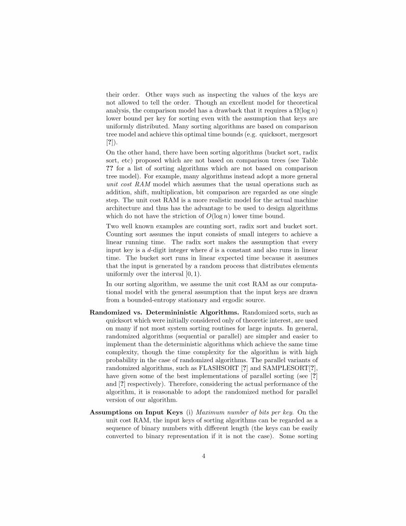
their order. Other ways such as inspecting the values of the keys arenot allowed to tell the order. Though an excellent model for theoreticalanalysis, the comparison model has a drawback that it requires a Ω(log n)lower bound per key for sorting even with the assumption that keys areuniformly distributed. Many sorting algorithms are based on comparisontree model and achieve this optimal time bounds (e.g. quicksort, mergesort[?]).

On the other hand, there have been sorting algorithms (bucket sort, radixsort, etc) proposed which are not based on comparison trees (see Table?? for a list of sorting algorithms which are not based on comparisontree model). For example, many algorithms instead adopt a more generalunit cost RAM model which assumes that the usual operations such asaddition, shift, multiplication, bit comparison are regarded as one singlestep. The unit cost RAM is a more realistic model for the actual machinearchitecture and thus has the advantage to be used to design algorithmswhich do not have the striction of O(log n) lower time bound.

Two well known examples are counting sort, radix sort and bucket sort.Counting sort assumes the input consists of small integers to achieve alinear running time. The radix sort makes the assumption that everyinput key is a d-digit integer where d is a constant and also runs in lineartime. The bucket sort runs in linear expected time because it assumesthat the input is generated by a random process that distributes elementsuniformly over the interval [0, 1).

In our sorting algorithm, we assume the unit cost RAM as our computa-tional model with the general assumption that the input keys are drawnfrom a bounded-entropy stationary and ergodic source.

Randomized vs. Determininistic Algorithms. Randomized sorts, such asquicksort which were initially considered only of theoretic interest, are usedon many if not most system sorting routines for large inputs. In general,randomized algorithms (sequential or parallel) are simpler and easier toimplement than the deterministic algorithms which achieve the same timecomplexity, though the time complexity for the algorithm is with highprobability in the case of randomized algorithms. The parallel variants ofrandomized algorithms, such as FLASHSORT [?] and SAMPLESORT[?],have given some of the best implementations of parallel sorting (see [?]and [?] respectively). Therefore, considering the actual performance of thealgorithm, it is reasonable to adopt the randomized method for parallelversion of our algorithm.

Assumptions on Input Keys (i) Maximum number of bits per key. On theunit cost RAM, the input keys of sorting algorithms can be regarded as asequence of binary numbers with different length (the keys can be easilyconverted to binary representation if it is not the case). Some sorting

4

algorithms, such as the algorithms based on data structure of digital searchtree (trie), and Radix Sort, assume that the number of bits per key isbounded by L. Radix Sort [?] requires O(L/log n) sequential work forsorting each key. The sorting algorithms using trie approach [?, ?] requiresO(log L) sequential work per key. However, the assumption of boundedmaximum length does not seem to hold widely in practice: in fact, manymajor users of sorting routines, e.g., data base joins, require moderatelylarge key size L. In our algorithm, we does not impose an upper boundon the maximum length of input keys. In other words, the running ofour algorithm is independent of the maximum length of the input keys.Instead, since we use prefix matching to find the order of the input keys,the complexity of the algorithms depends on the length of the first prefixmatch between two given keys.

(ii) Random input distribution vs. worst-case analysis. Another commonlyused assumption in sorting algorithm is to analyze the performance of thesorting algorithm based on certain distribution of the input, e.g. randomdistribution or worst case input. The apparent advantage of the worst-case input assumption is that the sorting time bound can be guaranteedeven in the worst case. As we illustrated in the introduction (see Chapter1), in practice the probability of sorting a worse case input is very small.On the other hand, if we assume random distribution of the inputs, inthe bucket sorting algorithm [?], sorting each key needs only O(1) ex-pected time. But the random input assumption also does not hold veryfrequently in practice as well. Therefore, we do not make assumption onthe probability distribution of the inputs, nor do we base our algorithmanalysis on the worst case inputs. Instead, we only assume that the inputkeys are drawn from a stationary and ergodic source with the underlyingprobability unknown before running the algorithm.

(iii) Entropy bounded input sets. As computer scientists, we would like todesign algorithms which are applicable to files found in practice. Thereforeit is a good question to ask what general properties of the practical inputswe can exploit to speed up the sorting algorithm. There have been vari-ous sorting algorithms which are not based on comparison-tree model andmake different assumptions about the input source. For example, Manilla[?] gave an optimal sorting algorithm by measuring presortedness of input.As discussed in the introduction of this thesis, for large files occurring inpractical applications, the lossless compression ratio is often at least 1.5and no more than a relatively small constant, say 20 (see definition of en-tropy and compression ratio in Chapter 1). It is not reasonable to assumeuniformly distributed sets of keys for practical files (otherwise, compres-sion ratio would almost always be 1, which is not the case), so bucket sortis not appropriate or at least has limited applicability for sorting largefiles in practice. Since the performance of our sorting algorithm depends

5

on the compressibility of the input keys, we will assume that the sourcefrom which the input keys are generated has a bounded compressibility.

Based on the above observations, we choose assumptions carefully for ournew sorting algorithm to suit the purpose of designing a practical sorting al-gorithm. We assume the randomized unit cost RAM as the computationalmodel. In order for the algorithm to have general applications (e.g., databasejoin applications). we assume no upper bound for maximum number of bitsthat each key can have. Since we utilize data structures and techniques usedin data compression algorithms, the time complexity of our algorithm dependson the compressibility of the input source. We assume that the compressibilityis bounded which is true for practical inputs so that the algorithm runs well inpractice.

1.1 Computational Model

Recall from the introduction that the unit cost RAM model we use allows thebasic operations such as addition, shift, and multiplication to be accomplishedin one single step. We regard the input keys as strings of binary bits. Ouranalysis depends on the total number of keys we are processing instead of thetotal number of bits the input has. Therefore, we assume no bound on themaximum length of a given input key. The actual machine memory layout ofthe key is irrelevant to the discussion of the algorithm. Specifically, we make thefollowing assumption to the computational model. Any input key x, representedby a binary string can be regarded as a binary number representing an integer.In other words, the input keys can also be viewed as a sequence of integers withno upper bound. This assumption is needed to insure that operation on triedata structure, such as finding the longest prefix match in the trie for a newkey, can be accomplished efficiently. We will describe in detail such operationsin next section.

1.2 Statistical Properties of Input Keys

We address the problem of relating the complexity of sorting to some statisti-cal properties of the input keys such as optimal compression ratio and entropy.Suppose the input source from which the input keys X1, X2, X3, ..., Xn are gen-erated is a stationary and ergodic sequence built over a binary alphabet 0,1.Recall from the introduction that informally, “ergodicity” means that as anysequence produced in accordance with a statistical source grows longer enough,it becomes entirely representative of the entire model. On the other hand, “sta-tionarity” means the underlying probability mass function of the input sourceis not changing over time

Let Xi, i = 1...n be the set of input keys which are generated by a sta-tionary source with the mixing condition. Recall from the introduction that a

6

X1 |–u(1)1 -|-u(2)

1 —–|-u(3)1 —|——

X2 |-u(1)2 –|-u(2)

2 —|-u(3)2 –|———

......Xn |—u

(1)n —|–u

(2)n —|-u(3)

n —–|–

Figure 1: Prefix matches of input keys.

sequence Xk∞1 is said to satisfy the mixing condition if there exists two con-stants c1 ≤ c2 and integer d such that for all 1 ≤ m ≤ m + d ≤ n the followingholds:

c1 Pr BPr C ≤ Pr BC ≤ qc2 PrBPrC (1)

where B ∈ Fm−∞ and C ∈ Fn

m+d. This mixing condition implies ergodicity of thesequence Xk∞−∞.

We now define Fn to be the input file of keys X1, X2, ..., Xn concatenatedtogether. In our algorithm, we only need to consider the first prefix matchof any given key to the dictionary. However, the definition of compressionratio is consistent with the compression ratio that we achieve when we considercompressing the concatenated file Fn, since Fn can also be viewed as generatedby the same statistical source. In Figure ?? below, Xi denotes the ith inputkey with arbitrary length and uj

i denotes the jth prefix match of the ith keyachieved by matching against the LZ dictionary (see section below for details).In our sorting algorithm, only the first prefix match u1

i will be involved in theanalysis of the algorithm.

Let L be the average length of the first prefix match, i.e., L = E(u(1)i ). The

optimal LZ code for n keys has log n bits [?]. Thus, the expected optimal com-pression ratio when we consider the sequence of concatenating u

(1)1 ,u(1)

2 ,u(1)3 ... is

Llog n as n→∞ [?]. However, as the whole input is generated from a stationary

and ergodic source, this compression ratio also limits to Llog n when we consider

compressing the input file Fn. Let H denote the entropy of the input source.We have the following lemma:

For large n as n→∞, H = Entropy(u(1)i ) = Entropy(Fn) for each i where

Fn is the concatenation of n input keys.

1.3 Random-Sampling Techniques

In our algorithm, a well known technique of randomization is used to make thealgorithm run efficiently in practice. Randomization has been successfully usedin a large number of applications and has recently been used to obtain efficientalgorithms in sorting. For example, sample sort [?] is a sorting algorithm usingrandom sampling techniques to adapt well to inputs with different distributions.

7

The general approach taken by random sampling algorithms is as follows.We randomly choose a subset R of the input set S to partition the problem intosmaller ones. The partitioned sub-problems can be proven to have a boundedsize with high likelihood. We then solve the sub-problems recursively usingknown techniques and form the solution of the whole problem based on thesolutions of the sub-problems. Clarkson [?] has proved that for a wide class ofproblems in algorithm design, the expected size of each subproblem is O(|S|/|R|)and more over the expected total size of the subproblem is O(|S|). Clarkson’sresults show that by using a straight-forward random sampling technique anyrandomly chosen subset is within the expected size with constant probability,implying that it may be not with constant probability. Consequently, his meth-ods yields expected resource bounds but cannot be used to obtain high-likelihoodbounds (i.e. the bounds that hold with probability greater than 1− nc for anyc > 0). This makes it very difficult to extend his methods to the context ofparallel algorithms.

Later a random sampling technique called over-sampling is introduced whichchooses s|R| number of splitters and then partitions the set into |R| groups sep-arating by the first key, the s-th key, the 2s-th key and so on. The numbers is called oversampling ratio. This technique overcomes the shortcomings ofClarkson’s method. Reif and Sen [?] also proposed a random sampling tech-nique called polling to obtain “good” samples with high probability with smalloverhead.

These random sampling techniques are especially useful for designing paral-lel algorithms where the primary goal is to distribute the work evenly across theprocessors. There has been extensive research on implementing various sortingalgorithms on parallel architectures [?, ?, ?]. Also various parallel sorting al-gorithms have been implemented on real parallel machine architectures. Therandom sampling techniques are used in parallel sorting to distribute the inputkeys to processors according to selected buckets where the size of each bucketis bounded within a constant of expected size with high likelihood. The mainadvantage is that the load balancing between processors can be achieved andthe parallel running time which depends on the longest running time of proces-sor can also be bounded. Reif and Sen [?] used random sampling techniquesto solve many parallel computation geometry problems (e.g. Voronoi diagram,trapezoidal decomposition) where the problems are divided into subproblemsby random sampling and the size of the subproblem is crucial to the parallelrunning time of the algorithm.

Another area in which the random sampling techniques are found useful isdesigning efficient algorithms whose performance depends on the distribution ofthe inputs. In these algorithms, the inputs are normally randomly subsampledin order to learn the underlying probability distribution of the inputs. Oursorting algorithm uses random sampling mainly as a tool to learn the unknownprobability distribution of the input source and use this information to aid ourcomputation.

8

2 Sequential Sorting Algorithm

Our sequential sorting algorithm consists of two phases. In the first phase, weuse randomized sampling technique to learn an approximation of the probabil-ity distribution of inputs. A digital search tree (trie) is constructed using thesampled keys in a way similar to the dictionary construction in LZ compression.The trie is used to reflex an approximation of the actual probability distribu-tion of the input keys. The trie is also used to partition the inputs into separatebuckets.

In the second phase, the input keys are indexed into buckets based on itsprefix match in the trie. We use a standard O(n log n) time sorting algorithm(e.g. quicksort) to sort each bucket separately and link buckets together usingtrie structure.

2.1 Trie Data Structure

The basic idea of our sorting algorithm is to divide the input keys almost evenlyinto partitioned buckets. We use a method similar to the construction of adictionary in LZ compression to index the input keys into buckets. It differsfrom the original dictionary construction in the way that the main purpose forour algorithm is approximating the unknown distribution of the input keys usingthe dictionary instead of actually compressing the inputs.

We now show how to build the dictionary D using a trie data structure(see Chapter 2 for a detailed presentation on trie). A trivial implementationof the trie is to use a simple binary tree whose nodes correspond to phrasesof the dictionary. However, the binary tree method is inefficient because thecomparison between an input key and the phrases in the tree is done only on abit-by-bit basis, taking O(L) time to find the maximum prefix match betweenthe key and trie where L is the length of the maximum prefix match.

In our algorithm, we adopt the hash table implementation of the trie wherecomparisons can be done more efficiently than the simple binary tree implemen-tation. Each phrase in the trie is now stored in a certain slot of the hash tablewhere the slot number is determined by a hash function. For the purpose of aclear presentation, we use the terminologies dictionary (in the context of datacompression), trie (the data structure) and hash table (the actual implementa-tion) interchangeably for the same data structure in the following descriptionof the algorithm.

We now show how to find the longest prefix match for each input key. Therunning time analysis is based on our assumption of the computational model.Specifically, we assume that any given key can be viewed as an integer andcomparison of integers and hash function computation can all be accomplishedin constant time. Let Ds be the current dictionary we have constructed. For anynew input key x, let Index(x) be the longest prefix of x that is already storedin the dictionary and dx is the length of Index(x). We can find Index(x) in

9

O(log d) time by searching in the hash table where di is the length of Index(xi)(see [?]). The basic idea of the search is that Index(xi) can be identified bydoubling the length of prefix of x for comparison each time (similar to binarysearch). Without loss of generality, we assume d = 2k (k is an intger) be thelength of the maximum prefix match of x. We first search in hash table to checkwhether the prefix consists of only the first character of x is already storedstored in the trie. This is done by computing the hash function h(x, 1) to findthe index number in the hash table where this character belongs. If we find thatthe first character is already stored in the hash table, we double the length ofthe prefix under inspection to check the prefix which consists of the first twocharacters of xi and so on. When we find that the prefix of length 2k+1 of xis not in the trie, we reverse the order of search using the same doubling (orsometimes halving) method to locate the longest prefix of x which is already inthe trie. Since the query of whether a given prefix is in the hash table can beanswered in constant time, the total search time depends on the length of thefirst prefix match. Specifically, we find the longest prefix match of input key xin O(log d) time where d is the length of the longest prefix match.

2.2 Description of the Algorithm

We are now ready to present the sequential sorting algorithm. We assume thebinary strings representing input keys are generated by the same stationaryand ergodic source whose probability distribution is initially unknown. Ouralgorithm consists of two phases. In the first phase, the unknown distributionof the inputs is learned by subsampling from the input and a dictionary is builtusing a trie structure from the sampled keys. In the second phase, all inputkeys are indexed to buckets associated with the leaves of the dictionary andeach bucket is sorted independently and then concatenated together to producethe output. A probabilistic analysis (Lemma ??) shows that the size of thelargest bucket can be bounded by O(log n/H) with high likelihood (by highlikelihood, we mean with probability ≥ 1 − 1/nΩ(1)). We also show that thesequential time complexity of this algorithm is expected to be O(n log log n),given that the input keys are not highly compressible, i.e., the compressionratio ρ ≤ (log n)O(1).

We present a randomized algorithm for sorting n keys X1, X2, ..., Xn. Inthe first phase, the distribution of the input keys is learned by building a datastructure similar to a dictionary used in LZ compression.

2.2.1 Random Sampling

First we randomly choose a set S of m = n/log n sample keys from the input keysand arrange them in random order. We will apply a modification of the usualLZ compression algorithm to construct a dictionary Ds from the first prefixesof the sample keys in S as described just below. The leaves of Ds represent the

10

set of points which partition the range of inputs into separate buckets accordingto the prefixes of input keys. Once Ds is constructed (and implemented byan efficient hash table [?]), we consider each key Xi for 1 ≤ i ≤ n and indexit to the corresponding bucket which is represented by leaves in the trie. LetXi = u

(1)i u

(2)i ... be the LZ prefix decomposition of Xi using the dictionary Ds.

Let u(1)i be the longest prefix of Xi that is already stored in the dictionary Ds.

2.2.2 Dictionary Construction

We now describe the construction of dictionary Ds. It is similar to original LZalgorithm except that we do not actually compress the input key. Ds will beincrementally constructed from an initially nearly empty set 0, 1 by findingthe first prefix match u

(1)si of each sampled key Xsi

(considered at random order)in the current constructed dictionary, and then adding the concatenation of u

(1)i

with first bit of u(2)i to the dictionary. This is different from the standard LZ

scheme as we stop processing this key now and go on to the next key. Eachstep takes time O(log |u(1)

si |) = O(log dsi). The main purpose of this dictionary

is to form an approximation of the probability distribution of the input sourceso that we can partition the range of input keys into buckets of nearly even size.

2.2.3 Indexing of Keys

Let a leaf of Ds be an phrase in Ds which is not a strict prefix of any otherphrases in Ds. Let LDs be the set of leaves in Ds (these are the leaves of thesuffix tree for Ds had it been explicitly constructed). Let Index(xi) be themaximal element of LDs which is lexicographically less than xi. Let di =lengthof Index(xi). Both u

(1)i and Index(xi) can be found in O(log di) sequential time

by using trie search techniques.

2.2.4 Sorting

After all keys have been indexed to the corresponding bucket, the buckets aresorted separately using a standard sorting algorithm (e.g. quicksort) and thenchained together according to the order of sample keys.

The sequential sorting algorithm is described as follows:

Sequential Sorting Algorithm

Input n keys X1, X2, ..., Xn, generated by a stationaryergodic source.

Output sorted n keys.

Step 1: Random samplingRandomly choose a set S of m = n/(log n) sample elementsfrom n input elements.

11

Step 2: Building buckets2.1 Randomly permute S = Xs1 , Xs2 , ..., Xsm.2.2 Construct the dictionary Ds as described.2.3 For each leaf wj of Ds (recall a leaf is an element

of Ds which is not a prefix of any other element of Ds),Bucket[wj ]← ∅.

Step 3: Indexing keysIndexing using Ds.for each key Xi, i = 1, ..., n do3.1 Use trie search to find the Index(Xi) (where

index is defined above).3.2 Insert Xi into the corresponding Bucket[Index(Xi)]

associated with the index of Xi.Step 4: Sorting4.1 Sort leaves of Ds using a standard sorting algorithm (e.g. Quicksort).4.2 Sort elements within each bucket using standard sorting

algorithm (e.g. Quicksort).4.3 All buckets are linked under the order of the sorted

leaves.

2.3 Analysis of Complexity

To bound the maximum size of the buckets, we have the following lemma: Thesize of each resulting bucket is O(log n/H) with probability ≥ 1− 1

nΩ(1) for largen where H is the entropy of the input source.

Proof: Recall that LDs is defined to be the set of leaves of dictionary Ds.In [?] it is shown that there exist c, c′ where c and c′ are two positive numberssuch that any leaf y ∈ LDs has probability between c/|LDs| and c′/|LDs| when|Ds| → ∞.

This result of [?] implies that for each key Xi (1 ≤ i ≤ n) with the sameprobability distribution, for each leaf y ∈ LDs, there exist constants c′′ and c′′′,such that

c′′/|LDs| ≤ Prob(y = Index(Xi)) ≤ c′′′/|LDs|.

Furthermore, [?, ?] shows that the size of the set of leaves |LDs| limits toH|Ds| for large |Ds|. Recall that in our algorithm |Ds| = |S| = O(n/ log n).Combine the above results and the fact that the the number of indexed keysfalling into a certain bucket follows binomial distribution, we conclude that thenumber of keys in

Bucket(y) = xi|Index(xi) = y

is less than O(log n/H) with probability ≥ 1− 1nΩ(1) . 2

We state the time complexity theorem of our algorithms as follows.The sorting algorithm takes O(n log( log n

H )) sequential expected running timewhere H is the entropy of the input keys.

12

Proof: Step 1 of the algorithm takes O(|S|) time where |S| = n/ log n isthe number of the sampled keys. In step 3, we define average length of the firstprefix match

L =Σn

i=1di

n(2)

Note that the optimal compression ratio ρ of the inputs is related to the expectedlength of first prefix match of the inputs such that

ρ =L

log n.

Also recall that searching the index of Xi takes O(log di) time where di is thelength of Index(Xi). Inserting key Xi into the corresponding bucket takes O(1)time. Therefore the time complexity for step 3 is Σn

i=1 log(di) = Σni=1 log(di) =

log Πni=1di ≤ log Ln = n log L = n log(ρ log n) = n log( log n

H ).Similarly, the time for step 2 can also bounded by n log(log n/H). Finally In

step 4, sorting leaves in Ds only takes time no more than O(n) as |S| = n/log nand |LDs| ≤ |S|. Then each bucket is sorted separately using a sorting algorithmwhich takes time O(ui log ui) for each bucket where ui is the size of the ithbucket. Note that

|LDs| ≤ |S| = n/log n.

By Lemma ??, the size of each bucket is bounded by O(log n/H) with highlikelihood, the expected time complexity of step 4 therefore is

T4 = Σ|LDs|i=1 ti

= Σ|LDs|i=1 ui log ui

≤ O(Σn/log ni=1 ui log(log n/H))

= O(n log( log nH )) as Σ|LDs|

i=1 ui = n.Thus, the total sequential time complexity of the algorithm is O(n log( log n

H )).2

We immediately have the following corollary assuming that the entropy Hof the input keys is bounded:

The algorithm takes O(n log log n) expected time if H ≥ 1(log n)O(1) .

2.4 Experimental Testing

We implemented the sequential version of our sorting algorithm on SPARC-2machine. The standard sorting algorithm we use for sorting the keys insideeach bucket is the Sun OS/4 system call qsort . We tested the algorithm on20 files with 24, 000 to 1, 500, 000 keys from a wide variety of sources, whosecompression ratios ranged from 2 to 4. We also derived an empirical formulafor the runtime bound of our algorithm. For comparison, we also did this for

13

Figure 2: Comparison of our sorting algorithm with Quick sort.

the UNIX system sorting routine - Quicksort. The results are shown in Figure??.

It is well know that the time of sorting each key using Quick sort can beexpressed in terms of the total number of keys: Tq = c0 + c1 log N . As wealready showed in the description of our sorting algorithm, the correspondingempirical formula for our sequential algorithm with fixed sample size is (regardthe entropy as a small constant): Te = d0 + d1 log log N .

We determined the constants using the experimental results:

c0 = 14.2, c1 = 1.68, d0 = 40.00, d1 = 3.73.

From the empirical formulas, it is easy to see that our sorting algorithm has alarger constant for the linear factor and that explains why our algorithm doesnot perform very well when the size of the input is small. The larger constant forthe linear factor is due to the large overhead caused by random sampling anddictionary indexing. However, the linear factor becomes less dominant whenthe size of the input grows large enough, as the formula shows. As predicted,our sorting algorithm performs better and better when the input size becomeslarger and larger. By extrapolation from these empirical tests we found oursequential sorting algorithm will beat quicksort when the total number of inputkeys N > 3.2× 107.

2.5 Discussion

In this section, we have presented the sequential sorting algorithm and its im-plementation. Like other non-trivial algorithms, our algorithms performs wellwhen the size of the input becomes large enough to cancel out the effect of largeoverhead. The major cost of any sorting algorithm is the time spent for any keyto decide its relative position in the whole input. Our basic idea is based onthis observation and we try to eliminate unnecessary comparisons by dividingkeys into ordered subgroups so that the only information needed for any keyto be sorted is to find its relative position in its subgroup. Since the input keyitself, especially its prefix, contains informations on which subgroup it belongsto, the preprocessing, or learning phrase of our algorithm uses this informationto index keys to buckets instead of redundant comparisons between two keys.

We utilize the trie data structure to execute string operations such as findingthe maximum prefix of any given key in the trie and inserting new phrases to thetrie. We also use the idea of constructing a dictionary using a method similarto dictionary construction in LZ compression. The dictionary we constructhas a nice property that it becomes a better and better approximation of theprobability distribution of the input source as it incrementally inserts more and

14

more input keys. Intuitively, if certain prefix has a high probability of appearingin input keys, there will be proportionally many input keys with this prefix thatare sampled. The dictionary will reflex the underlying probability distributionwith high likelihood if the number of input keys is large enough. Furthermore,as a property of the trie, the probability of an input key reaching to any leaf ofthe trie is about the same (see Lemma ??). This makes the task of finding agood partition of buckets especially easy.

Studies have indicated that sorting comprises about twenty percent of allcomputing on mainframes. Perhaps the largest use of sorting in computing(particularly in business computing) is the sort required for large database op-erations (e.g., required by joint operations). In these applications the keys havelength of many machine words. Since our sorting algorithm hashes the key(rather than compare entire keys as in comparison sorts such as quicksort), ouralgorithm is even more advantageous in the case of large key lengths in whichcase the cutoff is much lower. In case that the compression ratio is high (i.e.the input source is highly predictable), which can be determined after buildingthe dictionary, we just adopt the previous sorting algorithm, e.g., quick sort.

In later sections, we will demonstrate that the same techniques used in se-quential sort (trie data structure, fast prefix matching etc) can be extended toother problems (e.g., computational geometry problems) to decrease computa-tion by learning the distribution of the inputs.

3 Priority Queue Operations

A priority queue[?, ?, ?] is a data structure representing a single set S of ele-ments each with an associated value called a key. A priority queue supports thefollowing operations:Insert(S, x): insert the element x into the set S. This operation can be writtenas S ← S ∪ x.Max(S): return the element of S with the largest key.Extract-Max(S): remove and return the element of S with the largest key.

These operations can be executed on-line (i.e., in some arbitrary order andsuch that each instruction should be executed before reading the next one).The priority queues are useful in job scheduling and event-driven simulator. Insome applications, the operations Max and and Extract-Max are replaced byoperations Min and Extract-Min which returns the element with the smallestkey.

Our sequential algorithm can be modified to perform priority queue oper-ations. The bottleneck of the algorithm of [?] is the time for prefix matchingwhich depends on the maximum length of all possible keys. Applying our algo-rithm to build an on-line hash table which contains all the keys presently in thepriority queue, the time for prefix matching an arbitrary key can be reduced

15

to O(log log n/H) by searching through the hash tables. As an example, givena priority queue S and a key x to be inserted, we use the precomputed hashtable to search for the maximum prefix match for x in S. This effectively givesthe position of key x in S. We then proceed to insert x into S which takesconstant time once the position of x in the hash table is known. After key x isinserted into the trie, we use a pointer to link it to the key which is left neighborof x had all the keys been explicitly sorted (i.e. the biggest key in all the keysthat are smaller than x). The left neighbor can be identified in the process ofsearching. We keep a pointer pointing to the maximum key of the input keys.The Extract-Max operation can be performed in constant time by moving thepointer pointing to the maximum key to its left neighbor.

The time complexity of each operation does not depend on the length of thelongest input key. Instead, since the running time depends on the length of themaximum prefix match for any key in the priority queue, the complexity is onlyrelated to the entropy of input keys. We have the following corollary.

Assume that the input keys are generated by a stationary and ergodic sourcesatisfying mixing condition, the priority queue operations can be performed inO(log(log n/H)) expected sequential time where H is the entropy of input keys.2

4 Randomized Parallel Sorting Algorithm

The sequential sorting algorithm we presented was based on a divide and con-quer strategy. That is, the problem is divided into subproblem after learningcertain statistical properties of the input keys. The division of the subproblemsis carefully carried out so that the subproblems are of even size. The subprob-lems are then solved independently and the results are combined together toform the overall solution of the problem. Therefore, this parallalism underly-ing this algorithm can be utilized to design an efficient parallel version of ouralgorithm which will be presented in this section.

There has been extensive research and also implementations in the area ofparallel sorting. Reischuk [?] and Reif & Valiant [?] gave randomized sortingmethods that use n processors and run in O(log n) time with high probability.The first deterministic method to achieve such performance was an EREW com-parison PRAM algorithm based on the Ajtai-Komlos-Szemeredi sorting network.However, the constant factor in this time bound is still too large for practicaluse though it has an execution time of O(log n) using O(n) processors. Later,Bilardi & Nicolau [?] achieved the same performance with a practical small con-stant. Cole [?] also has given a practical deterministic method of sorting on anEREW comparison PRAM in time O(log n) using O(n) processors. Reif & Ra-jasekaran [?] presented an optimal O(log n) time PRAM algorithm using O(n)processors for integer sorting where key length is log n and Hagerup [?] gave anO(log n) time algorithm using O(n log log n/log n) processors for integer sorting

16

with a bound of O(log n) bits per key.List ranking problem is that given a singly linked list L with n objects, we

wish to compute, for each object, the distance from the end of the list. Theknown lower bound for list-ranking is Ω(log n/log log n) expected time (Beame &Hastad [?]) for all algorithms using polynomial number of processors on CRCWPRAM. If the results of the sorting algorithm are required to rank all the keysinstead of just a relative ordering of them, this lower bound applies to thesorting problems as well. However, in many problems only the relative orderinginformation of the keys is needed and the sorting algorithm does not include alist-ranking procedure at the end, the sorting can be accomplished much faster.If this is the situation, the sorted keys can be loosely placed in the final listwith empty places between any two of them. For example, [?] gives a PaddedSort (sorting n items into n + o(n) locations) algorithm which requires onlyΘ(log log n) time using n/log log n processors, assuming the items are takenfrom a uniform distribution.

We present a parallel version of our algorithm on CRCW PRAM model (seeintroduction for CRCW). We have the following theorem.

Let Lmax be the number of bits of the longest sample key. If Lmax ≤ nO(1),we get O(log n) expected time using O(n log( log n

H )/log n) processors for parallelsorting where H is the entropy of the input.

Proof: Assume that Lmax ≤ nO(1) and all keys are originally put in anarray A1 of length n.

The first part of our algorithm is indexing n keys to |LDs| buckets in parallelusing P = O(n log L

log n ) processors. There are log log n + 1 stages which we willdefine below.

Stage 0: here we do random subsampling of size n/log n from the n inputkeys, build up the hash table for indexing, precompute all random mappingfunctions for i = 1... log log n,

Ri : [1...ni]→ [1...ni]

where ni = n(c3)i for some constant c3 which will be determined below. All those

operations take O(log n) parallel time using O(n/log n) processors [?, ?].Stage 1: we arrange n keys in random order on an array with length n and

randomly assign O( log nlog L

) keys to each processor. Each processor j(1 ≤ j ≤ P )

then works on keys from (j−1) log nlog L

to j log nlog L

assigned to it separately for c0 log n

time where c0 is a constant greater than 1. In particular, each processor indexeskeys to buckets using the same technique described in our sequential algorithm.We can show at the end of this time there will be at most a constant factordecrease in the number of all keys left unindexed, say n/c1 where c1 > 1. Thenwe use the precomputed random mapping function R1 to map all keys to an-other array A1 with the same size of n which takes log n/log L time using Pprocessors. We now subdivide A1 into segments each with size c2 log n. Thena standard prefix computation is performed within each segment to delete the

17

already indexed keys which takes O(log log n) parallel time using n processors,so we can slow it down to O(log n) time using nlog log n/log n processors. Definec3 = c2/(1 + ε) where ε is a given constant say 1/3. The size of array A1 nowbecomes n/c3. Then we assign processor j keys from (j − 1) log n

c3 log Lto j log n

c3 log L.

To bound the number of unindexed keys per processor, we have the followinglemma :

The number of unindexed keys for each processor after random mappingis at most c2

c1log n(1 + ε) with probability 1 − 1/nΩ(1) for some small constant

ε(0 < ε < 1/2) and large c2.Proof: As the mapping function is random, the number U of unindexed

keys falling into a given segment in A2 is binomial distributed with probabil-ity 1/c1 and mean µ = c2

c1log n. Applying Chernoff Bounds (see [?] and also

introduction), we have

Pr(U ≥ c2c1

(1 + ε)log n) ≤ e−ε2µ2 = 1

nΩ(1)

for large c2 and given ε. 2

Stage i: now we apply all operations similar to those in stage 1 on thearray Ai−1. We assume Ai−1 has length n/(c3)i−1 and contains only remainingkeys still to be indexed. Each of these stages takes c0

(c3)i−1 log n time using P

processors. For example, now the prefix sum can be done in O(log log n) timeusing n

(c3)i−1 processors. So slowing down the time to O(log n)(c3)i−1 , we only need

nlog log n/log n processors which is less than P . All other time bounds areachieved similarly.

Repeat this stage until the number of keys left unindexed becomes n/log nwhich is less than P . Then we can finally assign each key a processor to finishthe job. The final work takes O(log n) time using P processors as long asLmax ≤ nO(1).

It is easy to see that the number of stages required is log log n. The totalparallel time complexity of these stages then is

O(Σlog log ni=0 (

1(c3)i

c0 log n)) ≤ O(log n)

.Next, we sort each bucket separately using a standard comparison based par-

allel sorting algorithm. Each bucket i of size Bi takes O(log Bi) time using O(Bi)processors. As each bucket size is bounded by O(log n/H) and Σ|LDs|

i=1 Bi = n,this sorting of buckets takes O(log(log n/H)) time using O(n) processors. Torelax the time bound to O(log n), we require O(n log(log n/H)

log n ) processors whichis upper bounded by P .

Finally, we use standard list-ranking algorithm to rank each key which takesonly O(log n) time using O(n/log n) processors (see [?]).

The initial construction of the dictionary Ds takes O(log n) time using Pprocessors by similar techniques. Thus, the total time is O(log n) using P

18

Figure 3: Two dimensional convex hull.

processors. 2

5 Application: Convex Hull Problem

In this section, we apply our sorting algorithm to a computational geometryproblem - the convex hull problem. We show that the efficient sorting algorithmcan improve the performance of convex hull algorithm with certain statisticalassumptions on the inputs.

The convex hull problem is defined as follows.Convex hull problem: Given a set of points in Ed (the Euclidean d-

dimensional space), find the smallest polygon containing these points.The sequential convex hull problem takes Ω(n log n) operations for n points

in two dimensions and there are algorithms with matching bound. However, Itis well known that the two dimensional convex hull problem can be solved inlinear time if the points are presorted by their x coordinates. Hence we have thefollowing corollary if we apply our sorting algorithm to sort the x-coordinatesof the input points:

Given a set of points, the two dimensional convex hull problem can besolved in O(n(log(log n/H))) sequential time where H is the entropy of thex-coordinates of the input points.

Since the sequential algorithm is straightforward, we are interested in design-ing an efficient parallel algorithm for the convex hull problem, using some wellknown techniques in parallel algorithm design. Below we present a parallel ver-sion of the algorithm for solving the two dimensional convex hull problem. Theinput is given as a set of n points represented by their polar coordinates (r, θ).We also assume that the set of points has a random distribution on the angularcoordinate θ while the radial coordinate r has an arbitrary distribution. Alsowe assume that the points have been presorted by their angular coordinates.The parallel machine model we use is CRCW PRAM.

First we choose independently O(log n) sets of random samples each of sizeO(nε) (ε is a small constant, say 1/3) and apply the polling technique of [?]to determine a good sample which divides the set into O(n1/3) sections (withrespect to θ) each with O(n2/3) points with probability ≥ 1− n−α where α is aconstant. The polling is done by chosing O(log2n) subsamples and testing for agood sample on a fraction n/(log n)O(1) of the inputs and it can be proven thatby applying the polling technique a good sample of the inputs can be obtainedwith high probability (refer to [?] for further details).

Within each section, the convex hull is constructed by applying recursivelythe merging procedure which we will describe below. This merging procedureis also applied to construct the final convex hull. The convex hull for the base

19

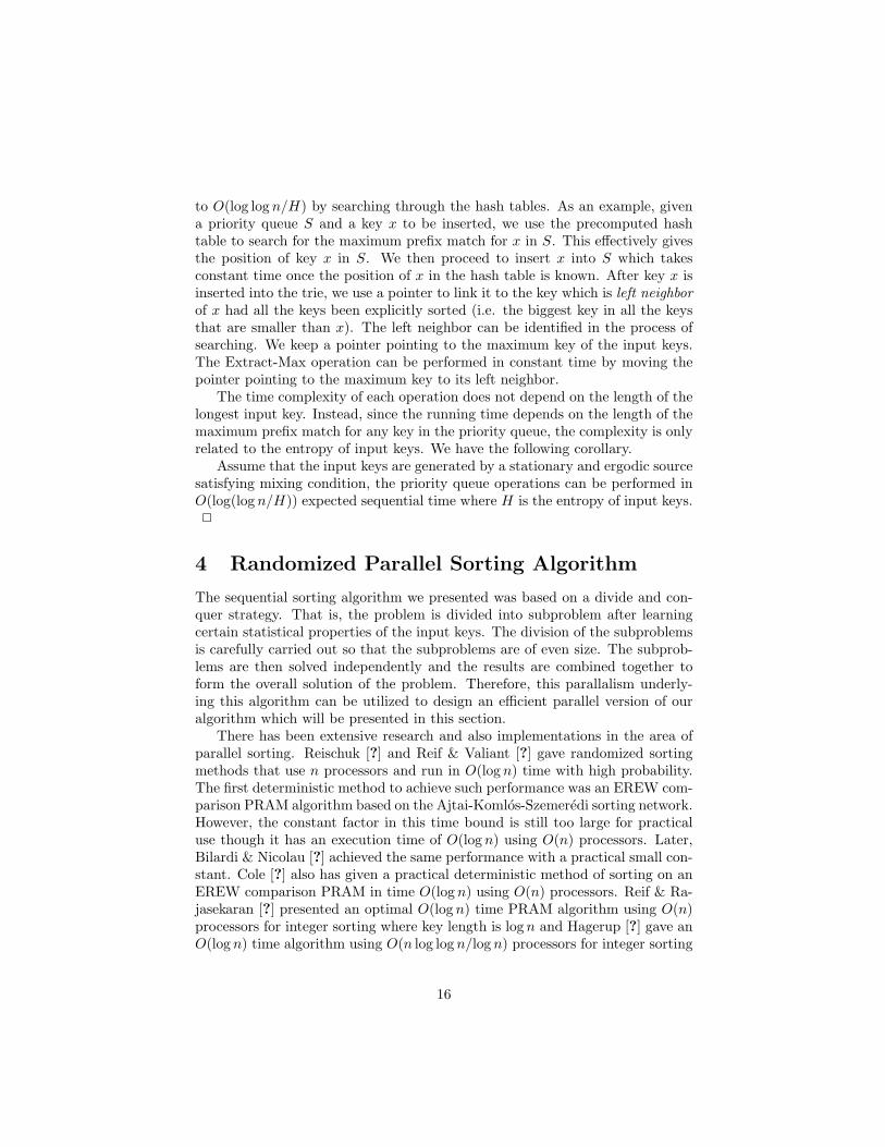
Figure 4: Finding common tangent in a refining process.

case where each section contains less than three points can be constructed inconstant time by a linear number of processors. We now describe the mergingprocedure (after constructing the convex hull of each section) in detail as follows:

Let ε′ be another small constant, say 1/9. We assign nε′ processors for eachpair of sections to find their common tangent. The total number of processorsused is (n1/3)2nε′ = O(n). As the problem of finding common tangent betweenany pair of sections are virtually the same, we focus our attention on only onepair of sections, say section i and j. However, all the common tangents betweenpairs of sections are to be found in parallel. Finding the common tangentbetween section i and j is carried out in a constant number of steps, precisely2/3ε′ steps. In the first step, we divide both sections into O(nε′) subsections and

solve the problem of finding the common tangent between these two sectionsafter we replace each part by the line segment linking its two endpoints (thepoints with minimum and maximum value of θ in the subsection). This problemcan be solved in constant time using the method discussed in [?] which findsthe common tangent in O(1) parallel time using a linear number of processors.

This common tangent (between subsection k in section i and subsection l insection j) we found is not exactly the one we need but very close because thereal common tangent (between section i and j) must go through subsection kand subsection l by the convex property (see Figure ??).

Then subsection k and l are further divided into nε′ parts. The size of theproblem is now reduced to O(n2/3−ε′). In the following steps, we apply the samemethod (O(1) time for each step) to refine the common tangent until we findthe one needed. The total time is still a constant.

After we find all the common tangents between pairs of sections, we constructthe convex hull by allocating edges of convex hull in a counter-clockwise direc-tion. For each section, find the common tangent with the minimum counter-clockwise angle with respect to the zero-degree line of the polar system. Thiscan be accomplished in O(1) time by assigning each section O(n2/3) processorsto find the minimum-angle common tangent on a CRCW PRAM [?].

So the merging step takes only O(1) time and O(n) processors. The timecomplexity for the parallel algorithm is therefore

T (n) = T (n2/3) + O(1) = O(log log n).

In each recursive step, the expected number of processors required is alwaysO(n). As the work in each recursive step is bounded by O(n) with high proba-bility, the total work for the parallel algorithm is thus O(n log log n) with highprobability ≥ 1− 1/nΩ(1).

The above algorithm can be summarized as follows:Given a set of two dimensional points represented by their polar coordinates

20

(r, θ) and assuming that the angular coordinates are presorted, the convex hull ofn points can be constructed in O(log log n) expected time using O(n) processors.

We immediately have the following corollary by applying our parallel sortingalgorithm to sort the angular coordinates of the input points:

Given a set of two dimensional points represented by their polar coordinates(r, θ) and let H be the entropy of the angular coordinates, the convex hull ofn points can be constructed in O((log(log n/H))) expected time using O(n)processors on CRCW PRAM. 2

6 Related Work

Following our entropy based sorting algorithm, Andersson and Nilsson [?] laterpresented a radix sort algorithm with improved time complexity. Their al-gorithm analyzes the complexity of the algorithm in terms of a more generalmeasurement, distinguishing prefixes. Specifically, their algorithm sorts a set ofn binary strings in Θ(n log( B

n log n + 2)) time, where B is the number of all dis-tinguishing prefixes, i.e., the minimum number of bits that have to be inspectedto distinguish the strings.

The distinguishing prefix is a more general measurement of difficulty of sort-ing than the entropy of the source from which the inputs are generated. Fora stationary ergodic process satisfying a certain mixing condition (see [?] fordetails), the following equation holds:

limn→∞

E(B)log n

=1H

.

Therefore, for any algorithm where the complexity can be expressed in termsof B, the complexity can be expressed in terms of entropy H as well. The reverseis not true for general inputs. Therefore, the approach analyzing the complexityof an algorithm in terms of distinguishing prefix is more general than one usingthe entropy of a stationary ergodic source.

However, it is noteworthy that their computational model used in the radixsort is different from ours in that their model assumes that rearranging thebinary strings (the input keys) can be all accomplished by moving pointers.Also, more importantly, their algorithm depends on the assumption that theexpected length of distinguishing prefix of each key is bounded by a constantmachine words, i.e. w = Ω(B), while our sorting algorithm does not depend onthis assumption. In fact, in our algorithm, the expected length of distinguishingprefix is O(log n/H) rather the length of a constant machine words. If we imposesuch assumptions, our algorithm runs in O(n) expected time.

21

7 Summary

In this chapter we investigated the first problem, sorting problem, in our study ofapplying data compression techniques to improve efficiency of algorithms. Aftera survey of previous work on sorting problem, we introduced a new randomizedsorting algorithm with certain statistical assumptions based on trie data struc-ture and binary string processing widely used in data compression algorithms.The algorithm was implemented and showed good performance comparing withsystem sorting routine. In addition, we gave a parallel version of the random-ized algorithm in the hope that the divide and conquer nature of our algorithmcan lay a solid ground for a highly parallel implementation. Finally we extendour method to convex hull problem to reduce the overall time complexity of thealgorithm to O(log(log n/H)).

Our primary motivation of the study of the sorting problem is not tryingto design a fastest sorting algorithm. Instead, we concentrated on studying theproblem of how to apply data structures and associated computational tech-niques to design efficient sorting algorithm and how to evaluate the validity ofcertain statistical assumptions on the input data and utilize these assumptionsto aid algorithm design. Also we presented several results in parallel settingsbecause the divide-and-conquer nature of our algorithm makes a parallel imple-mentation extremely attractive.

In the next chapter, we will study another fundamental algorithmic problem- string matching. The motivation to study string matching is the sheer impor-tance of this problem and its difference from the sorting algorithm. As sorting isan important operation in scientific computations, string matching is crucial inmany areas such as data processing, information retrieval and database design.Furthermore, unlike the sorting problem where the inputs are a set of indepen-dent keys, the string matching problem regards the input as a consecutive datastream. Thus a different approach in handling the input data is needed to designnew algorithms based on data compression ideas. Instead of applying certaindata structure in design of new algorithms, we will emphasize on how to analyzethe time complexity of a new algorithm based on statistical assumptions of theinputs.

References

[1] A. Amir and G. Benson. Efficient two dimensional compressed matching.Proc. of Data Compression Conference, Snow Bird, Utah, pages 279-288, Mar1992.

[2] A. Amir and G.Benson and M.Farach. Witness-free dueling: The perfectcrime! (or how to match in a compressed two-dimensional array). submittedfor publication, 1993.

22

[3] A. Amir and G. Benson and M. Farach. Let sleeping files lie: pattern match-ing in Z-compressed files. Symposium on Discrete Algorithms, 1994.

[4] A. Andersson and S. Nilson. A new efficient radix sort. 35th Symposium onFoundations of Computer Science, 714–721, 1994.

[5] S. Azhar and G. Badros and A. Glodjo and M.Y. Kao and J.H. Reif. DataCompression Techniques for Stock Market Prediction. Data CompressionConference, 1994.

[6] A.V. Aho and M.J. Corasick. Efficient string matching: and aid to biblio-graphic search. Communications of the ACM, Vol 18, 6:333-340, 1975.

[7] T.C. Bell, J.G. Cleary and I.H. Witten, Text Compression, Prentice HallPublisher, 1990.

[8] P. Beam and J. Hastad, Optimal bounds for decision problems on the CRCWPRAM, J.ACM, 36:643-670.

[9] P. Billingsley, Ergodic Theory and Information. John Wiley & Sons, NewYork 1965.

[10] P. Van Emade Boas, R. Kaas and E. Zulstra, Design and implementationof an efficient priority queue, Math. Systems. Theory, 10:99-127.

[11] G.E. Blelloch, C.E. Leiserson, B.M. Maggs, C.G. Plaxton, S.J. Smith andM. Zagha, A comparison of sorting algorithms for the Connection MachineCM-2, 3rd Annual ACM Symposium on Parallel Algorithms and Architecture,July 21-24, 1991.

[12] A. Bookstein and S.T. Klein and T. Raita and I.K. Ravichandra Rao andM.D. Patil, Can Random Fluctuation Be Exploited In Data Compression,Data Compression Conference, 1993.

[13] R.S. Boyer and J.S. Moore, A fast string searching algorithm, Communi-cations of the ACM, 20(10):762–772, 1977.

[14] G. Bilardi and A. Nicolau, Bitonic sorting with O(N log N) compar-sions, Proc.20th Ann. Conf. on Information Science and Systems, Princeton,NJ(1986)309-319.

[15] D. Bino and V. Pan. Polynomial and matrix computations, Vol 1,Birkhauser.

[16] R. Board and L. Pitt, On the Necessity of Occam Algorithms. Proceedingsof the 22nd Annual ACM Symposium on Theory of Computation, May 1990,pp 54-63.

23

[17] A. Borodin and P. Tiwari. On the Decidability of Sparse Univariate Poly-nomial Interpolation, Proc. 22nd Ann. ACM Symp. on Theory of Computing,535–545, ACM Press, New York, 1990.

[18] R.L. Baker and Y.T. Tse. Compression of high spectral resolution imagery.In Proceedings of SPIE: Applications of Digital Image Processing, pages 255–264, August 1988.

[19] P. Cignoni and L.D. Floriani and C. Montani and E. Puppo andR. Scopigno, Multiresolution modeling and visualization of volume data basedon simplicial complexes, Proceedings of Symposium on Volume Visualization,1994.

[20] R.J. Clarke, Transform coding of images, Academic Press, 1985.

[21] K.L. Clarkson, Applications of random sampling in computational geome-try ii. Proc of the 4th Annual ACM Symp on Computational Geometry, pages1–11, 1988.

[22] A. Czumaj and Z. Galil and L. Gasieniec and K. Park and W. Plandowski,Work-Time-Optimal Parallel Algorithms for String Problems, Syposium onTheoretical Computing, 1995.

[23] R. Cole and R. Hariharan. Tighter bounds on the exact complexity of stringmatching. 33th Symposium on Foundations of Computer Science, 600–609,1992.

[24] K. Curewitz,P. Krishnan and J.S. Vitter. Practical Prefetching via DataCompression, Proceedings of the 1993 SIGMOD International Conference onManagement of Data (SIGMOD ’93), Washington, D.C, May 1993, 257–266.

[25] M. Crochemore and L. Gasieniec and W. Rytter. Two-dimensional patternmatching by sampling. Information Processing Letters, 46:159–162, 1993.

[26] T.H. Cormen, C.E. Leiserson and R.L. Rivest, Introduction to algorithms,McGraw-Hill Book Company, 1990.

[27] R. Cole, Parallel merge sort, SIAM J.Comput, 17(1988)770-785.

[28] S. Chen and J. H. Reif. Using difficulty of prediction to decrease compu-tation: Fast sort, priority queue and computational geometry for bounded-entropy inputs. 34th Symposium on Foundations of Computer Science, 104–112, 1993.

[29] S. Chen and J. H. Reif. Fast pattern matching for entropy-bounded inputs.Data Compression Conference, 282–291, Snowbird, April, 1995.

[30] S. Chen and J.H. Reif. Survey on predictive computing. Duke Univ. Tech-nical Report No. CS–1995–14, October, 1995.

24

[31] S. Chen and J.H. Reif. Efficient lossless compression for trees and graphs.Data Compression Conference, Snowbird, 1996.

[32] S. Chen and J.H. Reif. Adaptive compression models for non-stationarysources. Manuscript, 1996.

[33] H. Chernoff. A measure of asymptotic efficiency for tests of a hypothesisbased on the sum of observations. Annuals of Mathematical Statistics, 23:493–507, 1952.

[34] T.M. Cover and J.A. Thomas, Elements of information theory, John Wiley& Sons, 1990.

[35] J.G. Cleary and I.H. Witten. Data compression using adaptive coding andpartial string matching. IEEE Tran. on Communications, 32:396–402, 1984.

[36] V. Cuperman. Efficient waveform coding of speech using vector quantiza-tion. PhD thesis, University of California, Santa Barbara, Feb 1983.

[37] J. Danskin and P. Hanrahan. Fast algorithms for volume ray tracing.Proceedings of the 1992 Workshop on Volume Visualization, pages 91–106,Boston, 1992.

[38] D. Dudgeon and R.Mersereau. Multidimensional Signal Processing.Prentice-Hall, N.J., 1984, pp.81, 82, 363–383

[39] C. Derman, Finite state Markov decision processes, Academic Press, NewYork, 1970.

[40] P. Van Emde Boas, Preserving order in a forest in less than logarithmictime and linear space, Information Processing Letters, volume 3, No.3, 1977.

[41] M. Farach and M.‘Noordewier and S. Savari and L. Shepp. On the En-tropy of DNA: Algorithms and Measurements based on Memory and RapidConvergence. SODA, 1995.

[42] T.R. Fischer and D.J. Tinnen. Quantized control with differential pulsecode modulation. In Conference Proceedings: 21st Conference on Decisionand Control, pages 1222-1227, December 1982.

[43] T.R. Fischer and D.J. Tinnen. Quantized control using differential encod-ing. Optimal Control Applications and Methods, pages 69-83, 1984.

[44] T.R. Fischer and D.J. Tinnen. Quantized control with data compressionconstraints. Optimal Control Applications and Methods, pages 593-596, May1982.

[45] Z. Galil. A constant-time optimal parallel string-matching algorithm. 24thSymposium on Theory of Computation, 69-76. 1992.

25

[46] R.G. Gallager. Variations on a theme by Huffman. IEEE Trans. on Infor-mation Theory, 24:668–674, 1978.

[47] J. Gil and Y. Matias, Fast hashing on a PRAM - Designing by expectation,Proc. 2nd. Ann. ACM Symp. on Discrete Algorithms.

[48] Z. Galil and Kunsoo Park. An improved algorithm for approximate stringmatching. SIAM J. Comput., Vol 19, 6:989-999, December 1990.

[49] Z. Galil and J. Seiferas, Time-space-optimal string matching. Journal ofcomputer and System Sciences, 26(3):280-294, 1983.

[50] R.M. Gray. Vector Quantization. IEEE ASSP Magazine, 1:4-29, April1984.

[51] R.M. Gray. Entropy and information theory. Sringer-Verlag, 1990.

[52] R.M. Gray. Source coding theory. Kluwer Academic Publishers, 1990.

[53] S. Gupta and A. Gersho. Feature predictive vector quantization of multi-spectral images, Trans. on Geoscience & remote sensing, 30(3):491-501, May1992.

[54] T. Hagerup, Towards optimal parallel bucket sorting, Inform. and Com-put., 75(1987)39-51.

[55] T. Hagerup and C.RUB, A guided tour of Chernoff bounds, InformationProcessing Letter 33(1989/90)305-308, North-Hollend.

[56] M.C. Harrison. Implementation of the substring test by hashing. Commu-nications of the ACM, 14:777-779, 1971.

[57] G. Held. Data compression, John Wiley & Sons, 1991.

[58] K.H. Holm. Graph matching in operational semantics and typing. InProceedings of Colloquium on Trees in Algebra and Programming, pages 191–205, 1990.

[59] J.S. Huang and Y.C. Chow, Parallel sorting and data partitioning bysampling, Proceedings of the IEEE Computer Society’s Seventh InternationalComputer Software and Applications Conference, 627-631, November 1983.

[60] W.L. Hightower, J.F. Prins and J.H. Reif, Implementations of randomizedsorting on large parallel machines, Symposium on Parallel Algorithm andArchitecture, 1992.

[61] D.A. Huffman, A method for the construction of minimum-redundancycodes, Proc. Institute of Electrical and Radio Engineering, 40 (9),1098-1101,September.

26

[62] J.JaJa, An introduction to parallel algorithm, Addison-Wesley, 1992.

[63] R.M. Karp and M.O. Rabin. Efficient randomized pattern-matching algo-rithms. Technical Report TR-31-81, Aiken Computation Laboratory, HarvardUniversity, 1981.

[64] D.E. Knuth, The art of computer programming, Volume 3, Sorting andsearching, Addison-Wesley, Reading, 1973.

[65] E. Karatsuba and Y.N. Lakshman and J.M. Wiley, Modular RationalSparse Multivariate Polynomial Interpolation, Proc. ACM-SIGSAM Int.Symp. on Symb. and Alg. Comp. (ISSAC ’90), 135–139, ACM Press, NewYork, 1990.

[66] D.E. Knuth and J.H. Morris and V.R. Pratt. Fast pattern matching instrings. SIAM J. Comput, 8:323-350, 1977.

[67] A.R. Karlin, S.J. Philips and P. Raghavan, Markov paging, Thirty-thirdAnnual Symposium on Foundations of Computer Science, Pittsburgh, Penn-sylvania,1992.

[68] P. Krishnan and J.S. Vitter, Optimal Prefetching in the worst case, Pro-ceedings of the 5th Annual SIAM/ACM Symposium on Discrete Algorithms,Alexandria, VA, January 1994.

[69] M. Levoy. Display of surface from volume data, IEEE Computer Graphicsand Applications, 8(3):29–37, 1988.

[70] J.S. Lim. Two Dimensional Image and Signal Processing Prentice-Hall,1990.

[71] P. Lacroute and M. Levoy. Fast volume rendering using a shear-warp fac-torization of the viewing transformation. Computer Graphics, 28(4):451–458,1994.

[72] T. Linder, G. Lugosi, and K. Zeger. Universality and rates of convergencein lossy source coding. preliminary draft, 1992.

[73] M. Li and P.M.B. Vitanyi. An introduction to Kolmogorov complexity andits applications Springer-Verlag, New York, Second Edition, 1997.

[74] M. Li and P.M.B. Vitanyi. On prediction by data compression, Proc.9th European Conference on Machine Learning, Lecture notes in artificialintelligence, Vol.XXX, Springer-Verlag, Heidelberg, 1997.

[75] M. Li and P.M.B. Vitanyi. Kolmogorov complexity arguments in combina-torics, J. Comb. Th.,, Series A, 66:2(1994), 226-236.

27

[76] T. Malzbender. Fourier volume rendering. ACM Transactions on Graphics,12(3):233–250, July 1993.

[77] M.R. Nelson, LZW data compression, Dr.Dobb’s Journal, October 1989.

[78] H. Mannila, Measures of Presortedness and Optimal Sorting Algorithms,IEEE Trans. Computers, 318-325, 1985

[79] S. Muthukrishnan and K. Palem. Highly efficient dictionary matching inparallel. extended abstract, 7:51–75, 1992.

[80] T. Markas and J. Reif. Multispectral image compression algorithms, InProceedings of 3rd Annual Data Compression Conference, pages 391–400,April 1993.

[81] T. Markas and J. Reif. Image compression methods with distortion controlcapabilities. In Proceedings of 1st Annual Data Compression Conference,pages 121–130, April 1991.

[82] P.D. MacKenzie and Q.F. Stout, Ultra-Fast Expected Time Parallel Algo-rithms, SODA Conference, 1991.

[83] Y. Matias and U. Vishkin, On parallel hashing and integer sorting, Proc.of 17th ICALP, Springer LNCS 443, 729-743, 1990.

[84] Y. Matias and J.S. Vitter and W.C. Ni. Dynamic Generation of DiscreteRandom Variates, Proceedings of the 4th Annual SIAM/ACM Symposium onDiscrete Algorithms, January 1993.

[85] V.S. Miller and M.N. Wegman, Variations on a theme by Ziv and Lempel,Combinatorial algorithms on words, edited by A.Apostolico and Z.Galil, 131-140, NATO ASI Series, Vol. F12., Springer-Verlag, Berlin.

[86] M. Palmer and S. Zdonik, “Fido: A Cache that Learns to Fetch,” Proceed-ings of the 1991 International Conference on Very Large Databases, Septem-ber 1991.

[87] B. Pittel, Asymptotical growth of a class of random trees, The Annals ofProbability, 1985, Vol 13, No.2. 414-427.

[88] W.B. Pennebaker and J.L. Mitchell. JPEG still image data compressionstandard. Van Nostrand Reinhold, 1992.

[89] P. Mcllroy, Optimistic Sorting and Information Theoretic Complexity,SPAA 93, 467-474, 1993.

[90] P. Raghavan, A statistical adversary for on-line algorithms, DIMACS Serieson Discrete Mathematics and Theoretical Computer Science, Vol 7, 1992.

28

[91] M.O. Rabin, Probabilistic algorithms, in J.F. Traub, ed. Algorithms andComplexity, pages 21–36, 1976.

[92] M. Rodeh, V.R. Pratt, and S. Even. Linear algorithm for data compressionvia string matching. J. of ACM, 28:1:16–24, 1981.

[93] S. Rajasekaran and J.H. Reif, Optimal and sublogarithmic time randomizedparallel sorting algorithms, SIAM J.Comput., 18:594-607, 1989.

[94] S. Rajasekaran and S. Sen, On parallel integer sorting, Acta Informatica,29, 1-15(1992).

[95] T. Raita and J. Teuhola. Predictive text compression by hashing. NewOrleans, LA.

[96] J. Reif, An optimal parallel algorithm for integer sorting, Proc.26th Ann.IEEE Symp. on Foundations of Computer Science (1985)496-504.

[97] J.H. Reif and S. Sen, Optimal randomized parallel algorithms for com-putational geometry. Proc. of the 16th International conference on ParallelProcessing, 1987.

[98] J.H. Reif and L.G. Valiant, A logarithmic time sort for linear size networks,Proc. 21st Ann. ACM Symp.on Theory of Computing (1989)264-273.

[99] R. Reischuk, A fast probabilistic sorting algorithm, SIAM J.Comput.,14(1985)396-409.

[100] F. Rubin. Experiments in text file compression. Communication of theACM, 19:11:617–623, 1976.

[101] P. Sabella. A rendering algorithm for 3d scalar fields. Computer Graphics,22(4):51–58, 1988.

[102] S. Sen, Random sampling techniques for efficient parallel algorithms incomputational geometry, Ph.D thesis, Duke University, 1989.

[103] R. Solovay and V.Strassen. A fast monte-carlo test for primality, SIAMJournal of Computing, 84–85, 1977.

[104] J.A. Storer, Data compression: methods and theory, Computer SciencePress, Rockvill, Maryland, 1988.

[105] D.D. Sleator and R.E. Tarjan. Amortized Efficiency of List Update andPaging Rules, Communications of the ACM, Vol 28, No.2, pp. 202-208, Febru-ary 1985.

[106] W. Szpankowski, A typical behavior of some data compression schemes,Data Compression Conference, 1991.

29

[107] W. Szpankowski, (Un)expected behavior of typical suffix trees, DataCompression Conference, 1991.

[108] Y. Shiloach and U. Vishkin, Finding the maximum, merging, and sortingin a parallel computation model, Journal of Algorithms 2:88-102(1981).

[109] C. Upson and M. Keeler. V-buffers: Visible volume rendering. ComputerGraphics, 22(4):59–64, 1988.

[110] J.S. Vitter and P. Krishnan, Optimal prefetching via data compression,In Journal of ACM, 43(5), September, 1996. A shortened version appeearsin Thirty-second Annual IEEE Symposium on Foundations of Computer Sci-ence, 1991.

[111] L.A. Westover. Splatting: a parallel, feed-forward volume rendering algo-rithm, Ph.D thesis, University of North Carolina, Department of ComputerScience, 1991.

[112] L. Westover, Footprint evaluation for volume rendering, Computer Graph-ics,, Volume 24, Number 4, August 1990.

[113] I.H. Witten and T.C. Bell and H. Emberson and S. Inglis and A. Mof-fat, Textual image compression: two-stage lossy/lossless encoding of textualimages, Proceedings of the IEEE, No.6, 1994.

[114] J. Wilhelms and A.V. Gelder. Muti-dimensional trees for controlled vol-ume rendering and compression, IEEE Proceedings of Symposium on volumevisualization, 1994.

[115] J. Ziv and A. Lempel, A universal algorithm for sequential data compres-sion, IEEE Trans. Information Theory, 23, 3, 337-343(1977).

[116] J. Ziv. Coding theorems for individual sequences, IEEE Trans. Informa-tion Theory, 24, 405-412(1978).

[117] A.C.C. Yao. The complexity of pattern matching for a random string.SIAM J.Comput, 8:3:368–387, 1979.

30