Using Garch Forecast Different in Stock Markets

Using the GARCH model to analyze and predict the different

stock markets Author：Wei Jiang

Supervisor: Lars Forsberg

2012/11/2

Master Thesis in Statistics Department of Statistics

Uppsala University Sweden

1

Using the GARCH model to analyze and predict the different

stock markets

December, 2012

Abstract

The aim of this article is to introduce several volatility models and use these models to predict

the conditional variance about the rate of return in different markets. This paper chooses the

GARCH model, E-GARCH model and GJR-GARCH model to analyze the rate of return and

considers using two different distributions on error terms: normal distribution and student-t

distribution. So this paper is mainly capturing the forecasting performance with volatility models

under different error distributions. Finally, after comparing the Root Mean Square Error (RMSE), choose the best model to predict the conditional variance. This paper selects five global stock

markets indexes: NASDAQ’s daily index, Standard and Poor’s 500 daily index, FTSE100 daily index, HANG SENG daily index and NIKKEI daily index. Key words: conditional variance; volatility models; error distribution; Root Mean Square Error (RMSE)

2

1. Introduction ...................................................................................................................... 4

2. Methodology .................................................................................................................... 4

2.1 ARCH model ................................................................................................................ 4

2.2 Generalized-ARCH (GARCH) model .............................................................................. 4

2.3 Exponential GARCH (EGARCH) model .......................................................................... 5

2.4 GJR-GARCH model....................................................................................................... 6

2.5 Distribution of the error term...................................................................................... 6

2.5.1 Normal distribution........................................................................................... 6

2.5.2 Student-t distribution ....................................................................................... 6

2.6 Root Mean Square Error (RMSE) ................................................................................. 7

3 Data................................................................................................................................ 7

3.1 NASDAQ analysis ......................................................................................................... 7

3.2 Standard & Poor 500 analysis ...................................................................................... 8

3.3 FTSE100 analysis ......................................................................................................... 8

3.4 NIKKEI analysis ............................................................................................................ 9

3.5 HANG SENG analysis ................................................................................................... 9

4 Results ........................................................................................................................ 11

4.1 Application in NASDAQ daily return........................................................................... 11

4.1.1 Selection of ARMA (p, q) model ...................................................................... 11

4.1.2 Result of GARCH model and GARCH family model for NASDAQ ....................... 11

4.2 Application in Standard &Poor 500 daily return ......................................................... 13


4.2.2 Result of GARCH model and GARCH family model for Standard &Poor 500 ..... 14

4.3 Application in FTSE100 daily return ........................................................................... 15

4.3.1 Selection of ARMA (p, q) model ..................................................................... 15

4.3.2 Result of GARCH model and GARCH family model for FTSE100 ........................ 16

4.4 Application in NIKKEI daily return .............................................................................. 17


4.4.2 Result of GARCH model and GARCH family model for NIKKEI .......................... 18

4.5 Application in HANG SENG daily return ..................................................................... 19


3

4.5.2 Result of GARCH model and GARCH family model for HANG SENG .................. 20

4.6 ARCH-LM test ............................................................................................................ 20

4.7 Out-of-sample forecasts ............................................................................................ 21

5 Conclusion .................................................................................................................... 24

6 Reference ..................................................................................................................... 25

6.1 Article resource ......................................................................................................... 25

6.2 Websites resource ..................................................................................................... 26

7 Appendix ...................................................................................................................... 27

4

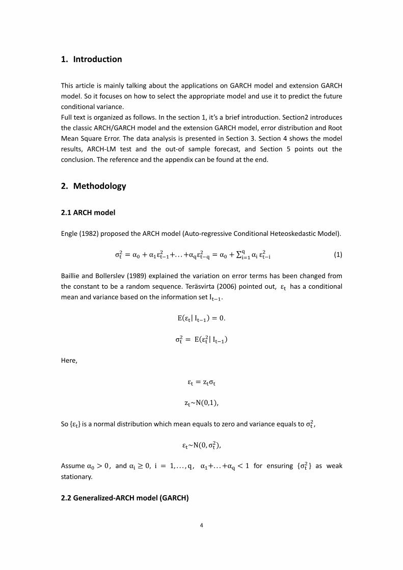
1. Introduction

This article is mainly talking about the applications on GARCH model and extension GARCH model. So it focuses on how to select the appropriate model and use it to predict the future conditional variance. Full text is organized as follows. In the section 1, it’s a brief introduction. Section2 introduces the classic ARCH/GARCH model and the extension GARCH model, error distribution and Root Mean Square Error. The data analysis is presented in Section 3. Section 4 shows the model results, ARCH-LM test and the out-of sample forecast, and Section 5 points out the conclusion. The reference and the appendix can be found at the end.

2. Methodology

2.1 ARCH model

Engle (1982) proposed the ARCH model (Auto-regressive Conditional Heteoskedastic Model). σ = α + α ε +. . . +α ε = α + ∑ α ε (1)

Baillie and Bollerslev (1989) explained the variation on error terms has been changed from the constant to be a random sequence. Teräsvirta (2006) pointed out, ε has a conditional mean and variance based on the information set Ι .

E(ε | Ι ) = 0.

σ = E(ε | Ι )

Here,

ε = z σ

z ~N(0,1),

So {ε } is a normal distribution which mean equals to zero and variance equals to σ ,

ε ~N(0, σ ), Assume α > 0 , and α ≥ 0, i = 1, . . . , q , α +. . . +α < 1 for ensuring {σ } as weak

stationary.

2.2 Generalized-ARCH model (GARCH)

5

Bollerslev (1986) and Taylor (1986) proposed the so-called generalized ARCH (GARCH) model for substituting the ARCH model.

σ = α + ∑ α ε + ∑ β σ (2)

Alexander and Lazar (2006) assume α > 0; α ≥ 0, i = 1, . . . , q;

β ≥ 0, j = 1, . . . , p; ∑ α + ∑ β < 1 for ensuring {σ } as weak stationary. Enocksson

and Skoog(2012) pointed out some limitations on GARCH model. The most important one is GARCH model cannot capture the asymmetric performance. Later, for improving this problem, Nelson (1991) proposed the EGARCH model and Glosten, Jagannathan and Runkel (1993) proposed GJR-GARCH model.

2.3 Exponential GARCH (EGARCH) model Nelson (1991) proposed the exponential GARCH (EGARCH) model.

logσ = c + ∑ g(Z ) + ∑ β log σ ,

Where,

g(Z ) = γ Z + α |Z | − E(|Z |)

Define Z = and the nature logarithm of the conditional variance equals to:

log(σ ) = c + ∑ β log σ + ∑ α − E + ∑ γ (3)

Alexander (2004) presented represents the symmetric effect, β measures the lagged conditional variance and reflects the asymmetric performance.

E(|Z |) =

⎩⎪⎨

⎪⎧ π

2, 푤ℎ푒푛 Z is normal distribution

√νΓ[0.5(ν − 1)]√πΓ(0.5ν)

, 푤ℎ푒푛 Z is student − t distribution�

Wang, Fawson, Barrett and Mcdonald (2001) demonstrate E(|Z |) is constant for all i

when Z is normal distribution or is√ [ . ( )]√ ( . ) depended on different when Z is

student-t distribution.

6

2.4 GJR-GARCH model

Glosten, Jagannathan and Runkle (1993) proposed GJR-GARCH model, another asymmetric model. Define the sequence {ε } equals to z σ and {ε } is a normal distribution.

ε ~N(0, σ )

So the GJR-GARCH model is written by

σ = c + ∑ β σ + ∑ α ε + ∑ γ ε I (ε < 0) (4)

In GJR-GARCH model, the sign of the indicator term captures the asymmetry and Patrick, Stewart and Chris (2006) describes it in details in their article.

I = 1, if ε < 0 0, otherwise

� ,

Where I is an indicator function, when the residual (ε ) is smaller than zero, the indicator term (I ) equals to one or equals to zero when the residual is not smaller than zero.

2.5 Distribution of the error term

This paper mainly introduces two distributions. One is normal distribution, the other one is student-t distribution. 2.5.1 Normal distribution

The probability density function of Z is given as follows,

f( Z ) =√

exp − ( μ) (5)

where is mean and is standard deviation. 2.5.2 Student t-distribution

The probability density function of Z is given as follows,

f( Z ) =ν

ν (ν )(1 +

ν) (ν ) (6)

Where is the number of degree of freedom, 2 < ν ≤ ∞, and is gamma function.

When ν → ∞, the student-t distribution nearly equals to the normal distribution. The lower

7

the , the fatter the tails.

2.6 Root Mean Square Error (RMSE)

Root Mean Square Error (RMSE) measures the difference between the true values and estimated values, and accumulates all these difference together as a standard for the predictive ability of a model. The criterion is the smaller value of the RMSE, the better the predicting ability of the model. This article uses this method to determine which model has the best forecasting performance. (http://en.wikipedia.org/wiki/Root-mean-square_deviation)

RMSE = ∑ (7)

where r is observed values and σ is the predicted value of conditional variance at time i, n is the number of forecasts.

3. Data

This paper uses the rate of return as data. So the stock returns should be required first by the following function: r = 100(ln(p ) − ln(p ) ), (8) where, r is the rate of returns for each stock index and p is the close price for each stock index at time t. 3.1 NASDAQ analysis

NASDAQ Stock Market Daily Closing Price Index is the first application which includes 1260 observations from the 2007-1-3 to 2011-12-30.

8

3.2 Standard & Poor 500 analysis

Standard & Poor 500 Stock Market Daily Closing Price Index is the second application which includes 1260 observations from the 2007-1-3 to 2011-12-30.

3.3 FTSE100 analysis

FTSE100 Stock Market Daily Closing Price Index is the third application, which includes 1263 observations from the 2007-1-2 to 2011-12-30.

-12

-8

-4

0

4

8

12

2007 2008 2009 2010 2011

The returns of NASDAQ daily close price index

NA

SD

AQ

's r

etur

ns

DATE

-12

-8

-4

0

4

8

12

2007 2008 2009 2010 2011

The returns of S&P500 daily close price index

DATE

S&

P50

0's

retu

rns

9

3.4 NIKKEI analysis

NIKKEI Stock Market Daily Closing Price Index is the forth application which includes 1221 observations from the 2007-1-4 to 2011-12-30.

3.5 HANG SENG analysis

HANG SENG Stock Market Daily Closing Price Index is the last application which includes

-10.0

-7.5

-5.0

-2.5

0.0

2.5

5.0

7.5

10.0

2007 2008 2009 2010 2011

The returns of FTSE100 daily close price index

FTS

E10

0's

retu

rns

DATE

-15

-10

-5

0

5

10

15

2007 2008 2009 2010 2011

The returns of NIKKEI daliy close price index

NIK

KE

I's

retu

rns

DATE

10

1261 observations from the 2007-1-2 to 2011-12-30.

The descriptions of different data

NASDAQ S&P500 FTSE100 HANG SENG NIKKEI

Sample size 1259 1259 1262 1260 1220

Min -9.5880 -9.4700 -9.2650 -13.5800 -12.1100

Max 11.1600 10.9600 9.3840 13.4100 13.2300

Mean 0.0058 -0.0095 -0.0099 -0.0077 -0.0589

SD 1.7443 1.6816 1.5484 2.0443 1.8463

Skewness -0.1839 -0.2449 -0.0824 0.0898 -0.5057

kurtosis 4.8702 6.5112 5.5156 5.9732 7.8186

Jarque-Bera 1257.7560 2246.9660 1608.9580 1883.7880 3173.7360

From this table, the skewness is -0.1839, -0.2449, -0.0824, 0.0898 and -0.5057. They are not zero which means all of the rates of returns are not symmetric. The kurtosis for different rate of returns is 4.8702, 6.5112, 5.5156, 5.9732 and 7.8186. They are larger than three, which means all stock returns have the fat-tail characteristic. Furthermore, the Jarque-Bera Test tells us the higher value represents the non-normality of the rate of returns. From the last line in the chart, all values are enough large (1257.7560, 2246.9660, 1608.9580, 1883.7880, 3173.7360), so the distributions of the rates of returns are not normal distribution. Next table is Box-Ljung test, which helps us to check whether the rate of returns has the ARCH effect or not, the null hypothesis is the rate of returns doesn’t have ARCH effect, while the alternative hypothesis is opposite. See Forsberg and Bollerslev (2002).

-15

-10

-5

0

5

10

15

2007 2008 2009 2010 2011

The returns of HANG SENG daily close price index

HA

NG

SE

NG

's r

etur

ns

DATE

11

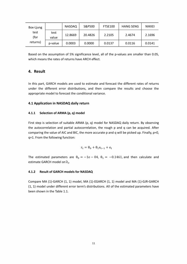
Box-Ljung test (for

returns)

NASDAQ S&P500 FTSE100 HANG SENG NIKKEI

test value

12.8669 20.4826 2.2105 2.4674 2.1696

p-value 0.0003 0.0000 0.0137 0.0116 0.0141

Based on the assumption of 5% significance level, all of the p-values are smaller than 0.05, which means the rates of returns have ARCH effect.

4. Result

In this part, GARCH models are used to estimate and forecast the different rates of returns under the different error distributions, and then compare the results and choose the appropriate model to forecast the conditional variance.

4.1 Application in NASDAQ daily return

4.1.1 Selection of ARMA (p, q) model First step is selection of suitable ARMA (p, q) model for NASDAQ daily return. By observing the autocorrelation and partial autocorrelation, the rough p and q can be acquired. After comparing the value of AIC and BIC, the more accurate p and q will be picked up. Finally, p=0, q=1. From the following function:

r = θ + θ e + e

The estimated parameters are θ = −1e − 04, θ = −0.1461, and then calculate and estimate GARCH model on e . 4.1.2 Result of GARCH models for NASDAQ Compare MA (1)-GARCH (1, 1) model, MA (1)-EGARCH (1, 1) model and MA (1)-GJR-GARCH (1, 1) model under different error term’s distributions. All of the estimated parameters have been shown in the Table 1.1.

12

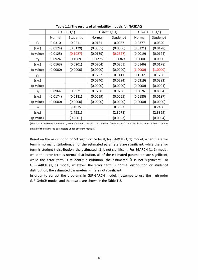
Table 1.1: The results of all volatility models for NASDAQ

GARCH(1,1) EGARCH(1,1) GJR-GARCH(1,1)

Normal Student-t Normal Student-t Normal Student-t

Ω 0.0310 0.0211 0.0161 0.0067 0.0377 0.0320

(s.e.) (0.0124) (0.0129) (0.0065) (0.0056) (0.0121) (0.0128)

(p-value) (0.0125) (0.1027) (0.0139) (0.2327) (0.0019) (0.0124)

α 0.0924 0.1069 -0.1275 -0.1369 0.0000 0.0000

(s.e.) (0.0163) (0.0201) (0.0204) (0.0251) (0.0146) (0.0178)

(p-value) (0.0000) (0.0000) (0.0000) (0.0000) (1.0000) (1.0000)

γ 0.1232 0.1411 0.1532 0.1736

(s.e.) (0.0240) (0.0294) (0.0319) (0.0393)

(p-value) (0.0000) (0.0000) (0.0000) (0.0004)

β 0.8964 0.8921 0.9768 0.9796 0.9026 0.8954

(s.e.) (0.0174) (0.0181) (0.0059) (0.0065) (0.0180) (0.0187)

(p-value) (0.0000) (0.0000) (0.0000) (0.0000) (0.0000) (0.0000)

ν 7.1875 8.3603 8.2400

(s.e.) (1.7931) (2.3078) (2.3369)

(p-value) (0.0001) (0.0003) (0.0004)

(This data is NASDAQ daily return, from 2007-1-3 to 2011-12-30 in yahoo finance, a total of 1259 observations. Table 1.1 points

out all of the estimated parameters under different models.)

Based on the assumption of 5% significance level, for GARCH (1, 1) model, when the error term is normal distribution, all of the estimated parameters are significant, while the error term is student-t distribution, the estimated is not significant. For EGARCH (1, 1) model, when the error term is normal distribution, all of the estimated parameters are significant, while the error term is student-t distribution, the estimated is not significant. For GJR-GARCH (1, 1) model, whatever the error term is normal distribution or student-t distribution, the estimated parameters α are not significant. In order to correct the problems in GJR-GARCH model, I attempt to use the high-order GJR-GARCH model, and the results are shown in the Table 1.2.

13

Table 1.2: The results of high-order GJR-GARCH model for NASDAQ

GJR-GARCH (2, 1) threshold=2




Ω 0.0481 0.0377 0.0704 0.0593 0.0190 0.0122

(s.e.) (0.0107) (0.0117) (0.0156) (0.0176) (0.0034) (0.0043)

(p-value) (0.0000) (0.0013) (0.0000) (0.0007) (0.0000) (0.0047)

α -0.0821 -0.0914 -0.0314 -0.0321 -0.1085 -0.1231

(s.e.) (0.0139) (0.0185) (0.0201) (0.0251) (0.0258) (0.0220)

(p-value) (0.0000) (0.0000) (0.1180) (0.1997) (0.0000) (0.0000)

α 0.0913 0.1072 0.1180 0.1363

(s.e.) (0.0268) (0.0364) (0.0259) (0.0260)

(p-value) (0.0007) (0.0032) (0.0000) (0.0000)

γ 0.1008 0.1242 0.0770 0.0946 0.1772 0.2378

(s.e.) (0.0358) (0.0446) (0.0446) (0.0531) (0.0380) (0.0416)

(p-value) (0.0048) (0.0054) (0.0844) (0.0748) (0.0000) (0.0000)

γ 0.0735 0.0524 0.2207 0.2211 -0.1155 -0.1914

(s.e.) (0.0443) (0.0551) (0.0431) (0.0531) (0.0397) (0.0461)

(p-value) (0.0969) (0.3411) (0.0000) (0.0000) (0.0036) (0.0000)

β 0.8802 0.8772 0.3255 0.3143 1.6215 1.6737

(s.e.) (0.0199) (0.0228) (0.1961) (0.2323) (0.0073) (0.0753)

(p-value) (0.0000) (0.0000) (0.0969) (0.1761) (0.0000) (0.0000)

β 0.5217 0.5276 -0.6708 -0.7154

(s.e.) (0.1800) (0.2116) (0.0015) (0.0645)

(p-value) (0.0038) (0.0127) (0.0000) (0.0000)

ν 10.1884 10.0496 10.2850

(s.e.) (2.8029) (2.8137) (2.7858)

(p-value) (0.0003) (0.0004) (0.0002)

(This data is NASDAQ daily return, from 2007-1-3 to 2011-12-30 in yahoo finance, a total of 1259 observations. This table points

out all of the estimated parameters under different higher-order GJR-GARCH models.)

Based on the assumption of 5% significance level, whatever the error term is normal distribution or student-t distribution, the estimated parameters of GJR-GARCH (2, 2) model are significant.

4.2 Application in Standard & Poor 500 daily return

4.2.1 Selection of ARMA (p, q) model

First step is selection of suitable ARMA (p, q) model for Standard & Poor 500 daily return. By observing the autocorrelation and partial autocorrelation, the rough p and q can be acquired. After comparing the value of AIC and BIC, the more accurate p and q will be picked up. Finally, p=1, q=1. From the following function:

14

r = θ + θ e + θ r + e

The estimated parameters are θ = −0.0093, θ = 0.2596, θ = −0.4000 , and then calculate and estimate GARCH model on e . 4.2.2 Result of GARCH models for Standard & Poor 500 Compare ARMA (1, 1)-GARCH (1, 1) model, ARMA (1, 1)-EGARCH (1, 1) model and ARMA (1, 1)-GJR-GARCH (1, 1) model under different error term’s distributions. All of the estimated parameters have been shown in the Table 2.1.

Table 2.1: The results of all volatility models for S&P500



Ω 0.0338 0.0213 0.0133 0.0062 0.0308 0.0222

(s.e.) (0.0108) (0.0121) (0.0059) (0.0070) (0.0093) (0.0096)

(p-value) (0.0018) (0.0781) (0.0231) (0.3789) (0.0010) (0.0212)

α 0.0994 0.1155 -0.1307 -0.1453 0.0000 0.0000

(s.e.) (0.0166) (0.0199) (0.0189) (0.0243) (0.0181) (0.0214)

(p-value) (0.0000) (0.0000) (0.0000) (0.0000) (1.0000) (0.9999)

γ 0.1240 0.1533 0.1478 0.1866

(s.e.) (0.0235) (0.0302) (0.0287) (0.0386)

(p-value) (0.0000) (0.0000) (0.0000) (0.0000)

β 0.8863 0.8835 0.9766 0.9812 0.9047 0.8984

(s.e.) (0.0176) (0.0181) (0.0053) (0.0062) (0.0186) (0.0177)

(p-value) (0.0000) 0.0000) (0.0000) (0.0000) (0.0000) (0.0000)

Ν 5.5449 5.6852 5.5915

(s.e.) (1.1064) (1.2529) (1.2337)

(p-value) (0.0000) (0.0000) (0.0000)

(This data is S&P500 daily return, from 2007-1-3 to 2011-12-30 in yahoo finance, a total of 1259 observations. This table points

out all of the estimated parameters under different models)

Based on the assumption of 5% significance level, for GARCH (1, 1) model, when the error term is normal distribution, all of the estimated parameters are significant, while the error term is student-t distribution, the estimated is not significant. For EGARCH (1, 1) model, when the error term is normal distribution, all of the estimated parameters are significant, while the error term is student-t distribution, the estimated is not significant. For GJR-GARCH (1, 1) model, whatever the error term is normal distribution or student-t distribution, the estimated parameters α are not significant. In order to correct the problems in GJR-GARCH model, I attempt to use the high-order GJR-GARCH model, and the results are shown in the Table 2.2.

15

Table 2.2: The results of high-order GJR-GARCH model for S&P500





Ω 0.0358 0.0234 0.0502 0.0305 0.0457 0.0267

(s.e.) (0.0059) (0.0070) (0.0083) (0.0091) (0.0085) (0.0094)

(p-value) (0.0000) (0.0009) (0.0000) (0.0008) (0.0000) (0.0044)

α -0.0736 -0.0878 -0.0519 -0.0548 -0.0727 -0.0876

(s.e.) (0.0132) (0.0182) (0.0187) (0.0243) (0.0156) (0.0188)

(p-value) (0.0000) (0.0000) (0.0056) (0.0242) (0.0000) (0.0000)

α 0.0626 0.0868 0.0483 0.0805

(s.e.) (0.0203) (0.0331) (0.0249) (0.0359)

(p-value) (0.0021) (0.0089) (0.0528) (0.0250)

γ 0.0653 0.0896 0.0730 0.0783 0.0715 0.0905

(s.e.) (0.0153) (0.0377) (0.0346) (0.0444) (0.0280) (0.0374)

(p-value) (0.0048) (0.0174) (0.0351) (0.0779) (0.0107) (0.0156)

γ 0.1273 0.1052 0.2430 0.2365 0.1908 0.1423

(s.e.) (0.0349) (0.0495) (0.0364) (0.0488) (0.0451) (0.0667)

(p-value) (0.0003) (0.0334) (0.0000) (0.0000) (0.0000) (0.0330)

β 0.8921 0.8891 0.2776 0.3647 0.5008 0.6847

(s.e.) (0.0166) (0.0007) (0.1243) (0.1908) (0.1903) (0.2948)

(p-value) (0.0000) (0.0000) (0.0255) (0.0560) (0.0085) (0.0202)

β 0.5836 0.5086 0.3630 0.1887

(s.e.) (0.1145) (0.1759) (0.1774) (0.2717)

(p-value) (0.0000) (0.0038) (0.0407) (0.4873)

ν 6.4932 6.6775 6.5236

(s.e.) (1.3690) (1.4516) (1.3793)

(p-value) (0.0000) (0.0000) (0.0000)

(This data is S&P500 daily return, from 2007-1-3 to 2011-12-30 in yahoo finance, a total of 1259 observations. This table points


Based on the assumption of 5% significance level, whatever the error term is normal distribution or student-t distribution, the estimated parameters of GJR-GARCH (2, 1) model are significant.

4.3 Application in FTSE100 daily return

4.3.1 Selection of ARMA (p, q) model First step is selection of suitable ARMA (p, q) model for FTSE100 daily return. By observing the autocorrelation and partial autocorrelation, the rough p and q can be acquired. After comparing the value of AIC and BIC, the more accurate p and q will be picked up. Finally, p=1, q=1. From the following function:

16

r = θ + θ e + θ r +e

The estimated parameters are θ = −0.01, θ = −0.7281 , θ = 0.6638, and then calculate and estimate GARCH model on e . 4.3.2 Result of GARCH model and GARCH family model for FTSE100 Compare ARMA (1, 1)-GARCH (1, 1) model, ARMA (1, 1)-EGARCH (1, 1) model and ARMA (1, 1)-GJR-GARCH (1, 1) model under different error term’s distributions. All of the estimated parameters have been shown in the Table 3.1.

Table 3.1: The results of all volatility models for FTSE100



Ω 0.0361 0.0364 0.0144 0.0089 0.0469 0.0441

(s.e.) (0.0135) (0.0158) (0.0071) (0.0073) (0.0127) (0.0138)

(p-value) (0.0073) (0.0209) (0.0231) (0.2239) (0.0002) (0.0014)

α 0.1292 0.1282 -0.1337 -0.1412 0.0000 0.0000

(s.e.) (0.0222) (0.0248) (0.0192) (0.0222) (0.0169) (0.0200)

(p-value) (0.0000) (0.0000) (0.0000) (0.0000) (1.0000) (1.0000)

γ 0.1499 0.1542 0.1888 0.1929

(s.e.) (0.0304) (0.0319) (0.0335) (0.0378)

(p-value) (0.0000) (0.0000) (0.0000) (0.0000)

β 0.8603 0.8622 0.9718 0.9723 0.8795 0.8781

(s.e.) (0.0215) (0.0236) (0.0075) (0.0080) (0.0202) (0.0217)

(p-value) (0.0000) (0.0000) (0.0000) (0.0000) (0.0000) (0.0000)

Ν 8.0252 10.6637 9.8946

(s.e.) (2.0368) (3.5244) (3.0625)

(p-value) (0.0001) (0.0025) (0.0012)

(This data is FTSE100 daily return, from 2007-1-2 to 2011-12-30 in yahoo finance, a total of 1262 observations. This table points


Based on the assumption of 5% significance level, for GARCH (1, 1) model, whatever the error term is normal distribution or student-t distribution, all of the estimated parameters are significant. For EGARCH (1, 1) model, when the error distribution is normal distribution, all of the estimated parameters are significant, while the error term is student-t distribution, the estimated is not significant. For GJR-GARCH (1, 1) model, whatever the error term is normal distribution or student-t distribution, the estimated parameters α are not significant. In order to correct the problems in GJR-GARCH model, I attempt to use the high-order GJR-GARCH model, and the results are shown in the Table 3.2.

17

Table 3.2: The results of high-order GJR-GARCH model for FTSE100





Ω 0.0443 0.0426 0.0652 0.0656 0.0263 0.0007

(s.e.) (0.0087) (0.0105) (0.0130) (0.0148) (0.0063) (0.0005)

(p-value) (0.0000) (0.0000) (0.0000) (0.0000) (0.0000) (0.1575)

α -0.0786 -0.0813 -0.0537 -0.0634 -0.0820 -0.0759

(s.e.) (0.0117) (0.0132) (0.0194) (0.0227) (0.0314) (0.0147)

(p-value) (0.0000) (0.0000) (0.0057) (0.0052) (0.0091) (0.0000)

α 0.0671 0.0656 0.0776 0.0757

(s.e.) (0.0198) (0.0222) (0.0310) (0.0147)

(p-value) (0.0007) (0.0031) (0.0124) (0.0000)

γ 0.2051 0.2131 0.1794 0.1895 0.2100 0.3272

(s.e.) (0.0493) (0.0558) (0.0405) (0.0442) (0.0502) (0.0499)

(p-value) (0.0000) (0.0001) (0.0000) (0.0000) (0.0000) (0.0000)

γ 0.0115 0.0143 0.1722 0.1953 -0.0908 -0.3200

(s.e.) (0.0516) (0.0585) (0.0387) (0.0442) (0.0634) (0.0481)

(p-value) (0.8242) (0.8064) (0.0000) (0.0000) (0.0152) (0.0000)

β 0.8824 0.8811 0.1763 0.1403 1.3338 1.8224

(s.e.) (0.0188) (0.0214) (0.1650) (0.1469) (0.0688) (0.0363)

(p-value) (0.0000) (0.0000) (0.2855) (0.3395) (0.0000) (0.0000)

β 0.6688 0.6960 -0.4019 -0.8260

(s.e.) (0.1478) (0.1317) (0.0626) (0.0354)

(p-value) (0.0000) (0.0000) (0.0000) (0.0000)

Ν 6.4932 12.5933 18.8548

(s.e.) (1.3690) (4.6137) (10.7172)

(p-value) (0.0000) (0.0063) (0.0785)

(This data is FTSE100 daily return, from 2007-1-2 to 2011-12-30 in yahoo finance, a total of 1262 observations. This table points


Based on the assumption of 5% significance level, when the error term is normal distribution, the estimated parameters of GJR-GARCH (2, 2) model are significant.

4.4 Application in NIKKEI daily return


First step is selection of suitable ARMA (p, q) model for NIKKEI return. By observing the autocorrelation and partial autocorrelation, the rough p and q can be acquired. After comparing the value of AIC and BIC, the more accurate p and q will be picked up. Finally, p=1, q=1. From the following function:

18

r = θ + θ e + θ r + e

The estimated parameters are θ = −0.0589, θ = −0.7306, θ = 0.6812 , and then calculate and estimate GARCH model on e . 4.4.2 Result of GARCH model and GARCH family model for NIKKEI

Compare ARMA (1, 1)-GARCH (1, 1) model, ARMA (1, 1)-EGARCH (1, 1) model and ARMA (1, 1)-GJR-GARCH (1, 1) model under different error term’s distributions. All of the estimated parameters have been shown in the Table 4.1.

Table 4.1: The results of all volatility models for NIKKEI



Ω 0.0625 0.0500 0.0204 0.0168 0.0547 0.0504

(s.e.) (0.0239) (0.0238) (0.0081) (0.0083) (0.0193) (0.0197)

(p-value) (0.0090) (0.0352) (0.0122) (0.0416) (0.0045) (0.0104)

α 0.1339 0.1203 -0.1134 -0.1125 0.0178 0.0170

(s.e.) (0.0231) (0.0235) (0.0165) (0.0177) (0.0175) (0.0183)

(p-value) (0.0000) (0.0000) (0.0000) (0.0000) (0.3091) (0.3516)

γ 0.1515 0.1494 0.1493 0.1450

(s.e.) (0.0341) (0.0342) (0.0291) (0.0306)

(p-value) (0.0000) (0.0000) (0.0000) (0.0000)

β 0.8496 0.8674 0.9773 0.9790 0.8854 0.8894

(s.e.) (0.0239) (0.0245) (0.0069) (0.0069) (0.0209) (0.0209)

(p-value) (0.0000) (0.0000) (0.0000) (0.0000) (0.0000) (0.0000)

Ν 13.5599 26.9464 26.9883

(s.e.) (6.0712) (20.6503) (23.9434)

(p-value) (0.0255) (0.1919) (0.2597)

(This data is NIKKEI daily return, from 2007-1-4 to 2011-12-30 in yahoo finance, a total of 1220 observations. This table points


Based on the assumption of 5% significance level, for GARCH (1, 1) model, whatever the error term is normal distribution or student-t distribution, all of the estimated parameters are significant. For EGARCH (1, 1) model, when the error term is normal distribution, the estimated parameters are significant, while the error term is student-t distribution, the is not significant. For GJR-GARCH (1, 1) model, the estimated parameters α and are not significant. In order to correct the problems in GJR-GARCH model, I attempt to use the high-order GJR-GARCH model, and the results are shown in the Table 4.2.

19

Table 4.2: The result of high-order GJR-GARCH model for NIKKEI





Ω 0.0745 0.0705 0.0254 0.0243 0.0903 0.0817

(s.e.) (0.0180) (0.0198) (0.0402) (0.0475) (0.0230) (0.0306)

(p-value) (0.0000) (0.0004) (0.5273) (0.6087) (0.0025) (0.0077)

α -0.0940 -0.1027 0.0111 0.0109 -0.0948 -0.1043

(s.e.) (0.0287) (0.0314) (0.0178) (0.0213) (0.0286) (0.0317)

(p-value) (0.0011) (0.0011) (0.5324) (0.6088) (0.0009) (0.0010)

α 0.1149 0.1237 0.1166 0.1254

(s.e.) (0.0285) (0.0329) (0.0293) (0.0338)

(p-value) (0.0001) (0.0002) (0.0001) (0.0002)

γ 0.2981 0.2716 0.2183 0.1951 0.2982 0.2762

(s.e.) (0.0428) (0.0481) (0.0382) (0.0445) (0.0427) (0.0480)

(p-value) (0.0000) (0.0000) (0.0000) (0.0000) (0.0000) (0.0000)

γ -0.1029 -0.0847 -0.1551 -0.1351 -0.0549 -0.0520

(s.e.) (0.0522) (0.0564) (0.1078) (0.1290) (0.0874) (0.0868)

(p-value) (0.0485) (0.1337) (0.1502) (0.2950) (0.5301) (0.5490)

β 0.8522 0.8563 1.4846 1.4945 0.5912 0.6368

(s.e.) (0.0222) (0.0235) (0.5603) (0.7040) (0.3317) (0.3471)

(p-value) (0.0000) (0.0000) (0.0081) (0.0338) (0.0747) (0.0665)

β -0.5368 -0.5452 0.2298 0.1959

(s.e.) (0.4807) (0.6082) (0.2895) (0.3053)

(p-value) (0.2641) (0.3700) (0.4273) (0.5211)

Ν 221305 24.0798 22.6387

(s.e.) (13.1145) (15.4397) (13.5151)

(p-value) (0.0915) (0.1189) (0.0939)

(This data is NIKKEI daily return, from 2007-1-4 to 2011-12-30 in yahoo finance, a total of 1220 observations. This table points


Based on the assumption of 5% significance level, when the error term is normal distribution, the estimated parameters of GJR-GARCH (2, 1) model are significant.

4.5 Application in HANG SENG daily return


First step is selection of suitable ARMA (p, q) model for HANG SENG return. By observing the autocorrelation and partial autocorrelation, the rough p and q can be acquired. After comparing the value of AIC and BIC, the more accurate p and q will be picked up. Finally, p=1, q=0. From the following function:

20

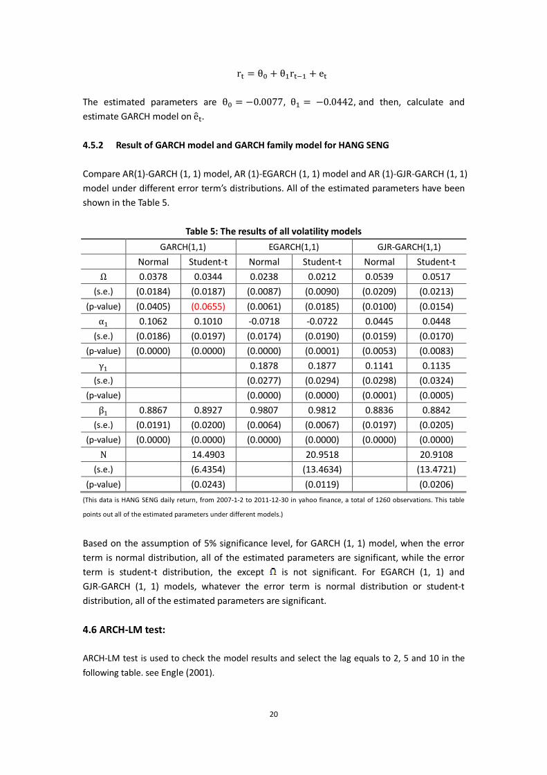
r = θ + θ r + e

The estimated parameters are θ = −0.0077, θ = −0.0442, and then, calculate and estimate GARCH model on e . 4.5.2 Result of GARCH model and GARCH family model for HANG SENG

Compare AR(1)-GARCH (1, 1) model, AR (1)-EGARCH (1, 1) model and AR (1)-GJR-GARCH (1, 1) model under different error term’s distributions. All of the estimated parameters have been shown in the Table 5.

Table 5: The results of all volatility models



Ω 0.0378 0.0344 0.0238 0.0212 0.0539 0.0517

(s.e.) (0.0184) (0.0187) (0.0087) (0.0090) (0.0209) (0.0213)

(p-value) (0.0405) (0.0655) (0.0061) (0.0185) (0.0100) (0.0154)

α 0.1062 0.1010 -0.0718 -0.0722 0.0445 0.0448

(s.e.) (0.0186) (0.0197) (0.0174) (0.0190) (0.0159) (0.0170)

(p-value) (0.0000) (0.0000) (0.0000) (0.0001) (0.0053) (0.0083)

γ 0.1878 0.1877 0.1141 0.1135

(s.e.) (0.0277) (0.0294) (0.0298) (0.0324)

(p-value) (0.0000) (0.0000) (0.0001) (0.0005)

β 0.8867 0.8927 0.9807 0.9812 0.8836 0.8842

(s.e.) (0.0191) (0.0200) (0.0064) (0.0067) (0.0197) (0.0205)

(p-value) (0.0000) (0.0000) (0.0000) (0.0000) (0.0000) (0.0000)

Ν 14.4903 20.9518 20.9108

(s.e.) (6.4354) (13.4634) (13.4721)

(p-value) (0.0243) (0.0119) (0.0206)

(This data is HANG SENG daily return, from 2007-1-2 to 2011-12-30 in yahoo finance, a total of 1260 observations. This table

points out all of the estimated parameters under different models.)

Based on the assumption of 5% significance level, for GARCH (1, 1) model, when the error term is normal distribution, all of the estimated parameters are significant, while the error term is student-t distribution, the except is not significant. For EGARCH (1, 1) and GJR-GARCH (1, 1) models, whatever the error term is normal distribution or student-t distribution, all of the estimated parameters are significant.

4.6 ARCH-LM test:

ARCH-LM test is used to check the model results and select the lag equals to 2, 5 and 10 in the

following table. see Engle (2001).

21

The ARCH-LM test of different models

p-value

ARCH-LM test

GARCH EGARCH GJR-GARCH


NADSAQ

Lag2 0.0804 0.0804 0.0432 0.0804

GJR-GAR

CH(2, 2)

GJR-GAR

CH(2, 2)

0.0594 0.0536

Lag5 0.3184 0.3184 0.0727 0.3184 0.1987 0.1269

Lag10 0.0501 0.0501 0.0425 0.0501 0.3116 0.2615

S&P500

Lag2 0.0721 0.2849 0.7605 0.4148

GJR-GAR

CH(2, 1)

GJR-GAR

CH(2, 1)

0.1278 0.1151

Lag5 0.7645 0.6748 0.8663 0.6570 0.3313 0.2162

Lag10 0.1518 0.3317 0.1004 0.3228 0.3180 0.2753

FTSE100

Lag2 0.2570 0.2951 0.0586 0.0588

GJR-GAR

CH(2, 2)

GJR-GAR

CH(2, 2)

0.0514 0.0520

Lag5 0.1381 0.1337 0.2259 0.2424 0.0929 0.0960

Lag10 0.3824 0.3788 0.4200 0.4437 0.2150 0.2237

HANG SENG

Lag2 0.6274 0.7320 0.2336 0.2366

GJR-GAR

CH(2, 1)

GJR-GAR

CH(2, 1)

0.1118 0.0800

Log5 0.0776 0.0598 0.0131 0.0131 0.0702 0.0547

Lag10 0.0830 0.0692 0.0131 0.0127 0.0559 0.0540

NIKKEI

Lag2 0.0721 0.0844 0.1315 0.2212

GJR-GAR

CH(1, 1)

GJR-GAR

CH(1, 1)

0.1768 0.2604

Lag5 0.0703 0.0509 0.0509 0.0986 0.3768 0.4778

Lag10 0.1232 0.0880 0.0958 0.0689 0.4732 0.5170

(This table represents the p-value of lag2, lag5 and lag10 under different applications.)

Based on the assumption of 5% significance level, when the result is larger than 0.05, which means the result doesn’t have ARCH effect, while the result still has ARCH effect when result is smaller than 0.05. From this table, S&P500, FTSE100 and NIKKEI, regardless of their models or error distribution, do not have ARCH effect, but NADSAQ and HANG SENG are not.

4.7 Out-of-sample Forecasts

In order to acquire the appropriate model to forecast the conditional variance, this paper use out-of-sample to calculate the root mean square error (RMSE), and the detail can be got from Forsberg and Bollerslev’s paper (2002). Here, use NASDAQ as an example to explain the process in details. The NASDAQ stock return includes 1259 observations, five years, and reserve the last year as out-of-sample, including

22

252 observations. Put in-sample data into a window, so the length of window is fixed which equals to 1007. First, pick up the observations from 1 to 1007 into this fixed window and use GARCH models to estimate and forecast. In this way, I get the first prediction conditional variance. This process is called as one-step-ahead forecast. Second, repeat the first step except pick up the observations from 2 to 1008 in the fixed window, and get the second prediction conditional variance. Next, repeat the first step except pick up the observations from 3 to 1009 in the fixed window, and get the third prediction conditional variance. Repeat this step 252 times. We call such a process as multi-step-ahead forecast. Finally, use the 252 prediction conditional variance to calculate the RMSE by the formula (7). Use this same method to deal with the other applications. Because the specific process is the same, so omit here and check the details from Appendix B.

23

Table 6：The result of RMSE about five different stock’s daily return

RMSE

NASDAQ GARCH (1,1)-Normal 5.4266

GARCH (1,1)-student-t 5.4559

EGARCH (1,1)-Normal 6.6210

EGARCH (1,1)-student-t 6.2907

GJR-GARCH (2,2)-Normal 5.3727

GJR-GARCH (2,2)-student-t 5.3980

RMSE

S&P500 GARCH (1,1)-Normal 4.9267






RMSE

FTSE100 GARCH (1,1)-Normal 3.3983






RMSE

HANG SENG GARCH (1,1)-Normal 5.2545






RMSE

NIKKEI GARCH (1,1)-Normal 8.6513






Boldfaced word represents the minimal value in each group. For each application, different models have different RMSE. For different applications, the model with minimal RMSE is also different.

24

5. Conclusion

This paper use different volatility models to analyze and forecast the conditional variance. At the same time, choose the normal distribution and the student-t distribution as the error term’s distribution. Table 6 illustrates which model has the smallest RMSE for different applications. Choose it as the best appropriate one to forecast the conditional variance. Different application has different appropriate model. For NASDAQ stock return, GJR-GARCH (2, 2) model under normal distribution has the smallest RMSE, so it will forecast the future conditional variance better than other models. For S&P500 stock return, GJR-GARCH (2, 1) model under normal distribution has the smallest RMSE, so it will predict the future conditional variance better than other models. For FTSE100 stock return, GJR-GARCH (2, 2) model under normal distribution has the smallest RMSE, so it will forecast the future conditional variance better than other models. For NIKKEI stock return, GJR-GARCH (1, 1) model under normal distribution has the smallest RMSE, so it will forecast the future conditional variance better than other models. For HANG SENG stock return, GARCH (1, 1) model under normal distribution has the smallest RMSE, so it will forecast the future conditional variance better than other models.

25

6. Reference

6.1 article resource

Alexander, C. and Lazar, E., 2006, Normal mixture GARCH (1, 1): application to exchange rate modeling. Journal of Applied Econometrics Economic Review, 39: 885–905. Alexander, C. and Lazar, E., 2004, The equity index skew, market crashes and asymmetric

normal mixture GARCH. ISMA Center Discussion Papers in Finance, 14. Andersen, T. G. and Bollerslev, T., 1998, Answering the skeptics: Yes, standard volatility

models provide accurate forecasts. International Economic Review, 39: 885-905.

Baillie, R. T. and Bollerslev, T., 1989, Common stochastic trends in a system of exchange rates. Journal of Monetary Economics, 44: 167-181.

Baillie, R. T., Bollerslev, T. and Mikkelsen, H. O., 1996, Fractionally integrated generalized autoregressive conditional heteroskedasticity. Journal of Econometrics, 74: 3-30.

Bollerslev, T., 1986, Generalized autoregressive conditional heteroskedasticity. Journal of Econometrics, 31: 307-327.

Bollerslev, T. and Mikkelsen, H. O., 1996, Modeling and pricing long memory in stock market volatility. Journal of Econometrics, Elsevier, vol. 73(1): 151-184.

Bollerslev, T., Chou, R. Y. and Kroner, K. F., 1992, ARCH modeling in finance: A review of the theory and empirical evidence. Journal of Econometrics, 52: 5-59.

Engle, R. F., 1982, Autoregressive conditional heteroscedasticity with estimates of the variance of United Kingdom inflation. Econometrics, 50: 987–1007.

Engle, R. F. and Bollerslev, T., 1986, Modeling the persistence of conditional variances, Econometric Reviews. Taylor and Francis Journals, vol. 5(1): 1-50.

Engle, R. F., 2001, GARCH 101: The use of ARCH/GARCH models in applied econometrics. Journal of Economic Perspectives, vol. 15(4): 157–168.

Engle, R. F., 2002, New frontiers For ARCH models. Journal of Applied Econometrics, 17: 425–446.

French, K. R., Schwert, G. W. and Stambaugh, R. F., 1987, Expected stock returns and volatility. Journal of Financial Economics, 19: 3–30.

Forsberg, L. and Bollerslev, T., 2002, Bridging the gap between the distribution of realized (ECU) volatility and ARCH modeling (of the EURO): the GARCH-NIG model. Journal of Applied Econometrics, 17: 535–548.

Franses, P. H. and Mcaleer, M., 2002, Financial volatility: An Introduction. Journal of Applied Econometrics, 17: 419–424.

Glosten, L., Jangannathan, R. and Runkle, D., 1993, On the relation between excepted value and the volatility of the nominal excess return of stocks. Journal of Finance, 48: 1779-1801.

He, C. and Teräsvirta, T., 1999, Properties of the autocorrelation function of squared observations for second order GARCH processes under two sets of parameter constraints. Journal of Time Series Analysis, 20: 23-30.

Nelson, D., 1991, Conditional heteroskedasticity in asset returns: a new approach. Econometrics, 59: 349–370.

26

Nelson, D. B. and Cao, C. Q., 1992, Inequality constraints in the univariate GARCH model. Journal of Business and Economic Statistics, 10: 229-235.

Patrick, D., Stewart, M. and Chris. S., 2006, Stock returns, implied volatility innovations, and the asymmetric volatility phenomenon. Journal of Financial and Quantitative Analysis, 41: 381-406.

Rabemananjara, R. and Zakoian, J. M., 1993, Threshold Arch Models and Asymmetries in Volatility. Journal of Applied Econometrics, 8(1): 31–49.

Teräsvirta, T., 2006, An introduction to univariate GARCH models, SSE/EFI. Working Papers in Economics and Finance, No. 646.

Wang, K. L., Fawson, C., Barrett, C. B. and Mcdonald, J. B., 2001, A flexible parametric GARCH model with an application to exchange rates. Journal of Applied Econometrics, 16: 521–536.

6.2 websites resource Wikipedia: Root-mean-square deviation,

http://en.wikipedia.org/wiki/Root-mean-square_deviation

Yahoo finance: S&P500 historical prices, http://finance.yahoo.com/q/hp?s=%5EGSPC+Historical+Prices

Yahoo finance: NASDAQ historical prices, http://finance.yahoo.com/q/hp?s=%5EIXIC+Historical+Prices

Yahoo finance: FTSE100 historical prices, http://finance.yahoo.com/q/hp?s=%5EFTSE+Historical+Prices Yahoo finance: HANG SENG historical prices,

http://finance.yahoo.com/q/hp?s=%5EHSI+Historical+Prices Yahoo finance: NIKKEI historical prices,

http://finance.yahoo.com/q/hp?s=%5EN225+Historical+Prices

27

7. Appendix:

In the same way, the S&P500 stock return includes 1259 observations, five years, and reserve the last year as out-of-sample, including 252 observations. Put in-sample data into a window, so the length of window is fixed which equals to 1007. First, pick up the observations from 1 to 1007 into this fixed window and use GARCH models to estimate and forecast. In this way, I get the first prediction conditional variance. This process is called as one-step-ahead forecast. Second, repeat the first step except pick up the observations from 2 to 1008 in the fixed window, and get the second prediction conditional variance. Next, repeat the first step except pick up the observations from 3 to 1009 in the fixed window, and get the third prediction conditional variance. Repeat this step 252 times. We call such a process as multi-step-ahead forecast. Finally, use the 252 prediction conditional variance to calculate the RMSE by the formula (7). With the same method, the FTSE100 daily return includes 1262 observations, five years, and reserve the last year as out-of-sample, including 251 observations. Put in-sample data into a window, so the length of window is fixed which equals to 1011. First, pick up the observations from 1 to 1011 into this fixed window and use GARCH models to estimate and forecast. In this way, I get the first prediction conditional variance. This process is called as one-step-ahead forecast. Second, repeat the first step except pick up the observations from 2 to 1012 in the fixed window, and get the second prediction conditional variance. Next, repeat the first step except pick up the observations from 3 to 1013 in the fixed window, and get the third prediction conditional variance. Repeat this step 251 times. We call such a process as multi-step-ahead forecast. Finally, use the 251 prediction conditional variance to calculate the RMSE by the formula (7). Next, the HANG SENG daily return includes 1260 observations, five years, and reserve the last year as out-of-sample, including 251 observations. Put in-sample data into a window, so the length of window is fixed which equals to 1009. First, pick up the observations from 1 to 1009 into this fixed window and use GARCH models to estimate and forecast. In this way, I get the first prediction conditional variance. This process is called as one-step-ahead forecast. Second, repeat the first step except pick up the observations from 2 to 1010 in the fixed window, and get the second prediction conditional variance. Next, repeat the first step except pick up the observations from 3 to 1011 in the fixed window, and get the third prediction conditional variance. Repeat this step 251 times. We call such a process as multi-step-ahead forecast. Finally, use the 251 prediction conditional variance to calculate the RMSE by the formula (7). Last, the NIKKEI daily return includes 1220 observations, five years, and reserve the last year as out-of-sample, including 244 observations. Put in-sample data into a window, so the length of window is fixed which equals to 976. First, pick up the observations from 1 to 976 into this fixed window and use GARCH models to estimate and forecast. In this way, I get the first prediction conditional variance. This process is called as one-step-ahead forecast. Second, repeat the first step except pick up the observations from 2 to 977 in the fixed window, and get the second prediction conditional variance. Next, repeat the first step except pick up the observations from 3 to 978 in the fixed window, and get the third prediction conditional variance. Repeat this step 244 times. We call such a process as

28

multi-step-ahead forecast. Finally, use the 244 prediction conditional variance to calculate the RMSE by the formula (7).

Using Garch Forecast Different in Stock Markets

Documents

Transcript of Using Garch Forecast Different in Stock Markets