The Stock Returns Volatility based on the GARCH (1,1 ...
22
Iran. Econ. Rev. Vol. 23, No. 1, 2019. pp. 87-108 The Stock Returns Volatility based on the GARCH (1,1) Model: The Superiority of the Truncated Standard Normal Distribution in Forecasting Volatility Emrah Gulay *1 , Hamdi Emec 2 Received: 2018, January 3 Accepted: 2018, Febuary 1 Abstract n this paper, we specify that the GARCH(1,1) model has strong forecasting volatility and its usage under the truncated standard normal distribution (TSND) is more suitable than when it is under the normal and student-t distributions. On the contrary, no comparison was tried between the forecasting performance of volatility of the daily return series using the multi-step ahead forecast under GARCH(1,1) ~ TSND and GARCH(1,1) ~ normal and student-t distributions, until lately, to the best of my understanding. The findings of this study show that the GARCH(1,1) model with the truncated standard normal distribution gives encouraging results in comparison with the GARCH(1,1) with the normal and student-t distributions with respect to out-of-sample forecasting performance. From the empirical results it is apparent that the strong forecasting performances of the models depend upon the choice of an adequate forecasting performance measure. When the one-step ahead forecasts are compared with the multi-step ahead forecasts, the forecasting ability of the former GARCH(1,1) models (using one-step ahead forecast) is superior to the forecasting potential of the latter GARCH(1,1) model (utilizing the multi-step ahead forecast). The results of this study are highly significant in risk management for the short horizons and the volatility forecastability is notably less relevant at the longer horizons. Keywords: Volatility, Financial Time Series, Truncated Standard Normal Distribution, ARCH/GARCH Models, Forecasting. JEL Classification: C53, C58. 1. Introduction In our contemporary world, stock markets represent an essential and active component of the financial markets. Heightened competition in 1. Faculty of Economics and Administrative Sciences, Department of Econometrics, Izmir, Turkey (Corresponding Author: [email protected]). 2. Faculty of Economics and Administrative Sciences, Department of Econometrics, Izmir, Turkey ([email protected]). I
Transcript of The Stock Returns Volatility based on the GARCH (1,1 ...
Iran. Econ. Rev. Vol. 23, No. 1, 2019. pp. 87-108
The Stock Returns Volatility based on the GARCH (1,1)
Model: The Superiority of the Truncated Standard
Normal Distribution in Forecasting Volatility
Emrah Gulay*1, Hamdi Emec2
Received: 2018, January 3 Accepted: 2018, Febuary 1
Abstract n this paper, we specify that the GARCH(1,1) model has strong
forecasting volatility and its usage under the truncated standard
normal distribution (TSND) is more suitable than when it is under the
normal and student-t distributions. On the contrary, no comparison was
tried between the forecasting performance of volatility of the daily
return series using the multi-step ahead forecast under GARCH(1,1) ~
TSND and GARCH(1,1) ~ normal and student-t distributions, until
lately, to the best of my understanding. The findings of this study show
that the GARCH(1,1) model with the truncated standard normal
distribution gives encouraging results in comparison with the
GARCH(1,1) with the normal and student-t distributions with respect to
out-of-sample forecasting performance. From the empirical results it is
apparent that the strong forecasting performances of the models depend
upon the choice of an adequate forecasting performance measure. When
the one-step ahead forecasts are compared with the multi-step ahead
forecasts, the forecasting ability of the former GARCH(1,1) models
(using one-step ahead forecast) is superior to the forecasting potential of
the latter GARCH(1,1) model (utilizing the multi-step ahead forecast).
The results of this study are highly significant in risk management for
the short horizons and the volatility forecastability is notably less
relevant at the longer horizons.
Keywords: Volatility, Financial Time Series, Truncated Standard
Normal Distribution, ARCH/GARCH Models, Forecasting.
JEL Classification: C53, C58.
1. Introduction
In our contemporary world, stock markets represent an essential and
active component of the financial markets. Heightened competition in
1. Faculty of Economics and Administrative Sciences, Department of Econometrics, Izmir, Turkey (Corresponding Author: [email protected]). 2. Faculty of Economics and Administrative Sciences, Department of Econometrics, Izmir, Turkey ([email protected]).
I
88/ The Stock Returns Volatility based on the ...
the financial markets has increased the significance of prediction of
the volatility of stock prices, as evident from several studies
conducted over the prior decade. In keeping with the technological
advancements, computer programming and data mining techniques
extensively employ stock price predictions. In the meantime, it is clear
that approaches like artificial neural networks, are utilized as well
(Koutrou Manidis et al., 2011). However, dependence on the stock
price history and ignorance of other relevant information on market
volatility can be understood as the vulnerable points to these
approaches.
The statistical analyses on the time series concentrated on the
conditional first moment. The expanding role of risk and uncertainty
in decision-making models and, in the meanwhile, changes in
assessing the risk and volatility measurements over the specified time,
enabled the development of new time series methods for the modeling
of the second moment, for the analysis of the time series data. The
Autoregressive Conditional Heteroskedasticity (ARCH) and
Generalized Autoregressive Conditional Heteroskedasticity (GARCH)
models deal with the dependence of the conditional second moment;
they also make significant contributions to modeling these processes
which are characterized by a high degree of fluctuation. Specifically,
they are commonly practiced in the analysis of the financial time
series in revealing the heavy-tailed distribution (Teresiene, 2009).
Earlier contributions to the literature which considered the lack of
predictive capability of the GARCH models include Tse (1991), Kuen
and Hoong (1992), Terasvirta (1996), He and Terasvirta (1999), and
Malmsten and Terasvirta (2004). These papers emphasize that the
GARCH(1,1) model may not show a better forecasting performance,
and does not capture several of the characteristic properties of the
financial time series. Goyal (2000) in his investigations on the
performance of some GARCH models showed that the GARCH-M
(GARCH in the Mean) model exhibits poor out-of-sample forecasting
performance when compared with the ARMA specification. Hansen
and Lunde (2005) examined 330 different ARCH (GARCH) models to
test if any of these models could surpass the performance of the
GARCH(1,1) model. They indicated that the GARCH(1,1) model was
not superior to any of the more complex models by using exchange

Iran. Econ. Rev. Vol. 23, No.1, 2019 /89
data. However, Andersen and Bollerslev (1998); Christodoulakis and
Satchell (1998; 2005) highlighted examples of the poor out-of-sample
forecasting performance of the GARCH models that is skeptical
because of utilizing the squared shocks as a proxy for the true
unobserved conditional variance. From studies available in the
literature, it is evident that the forecasting ability of the GARCH models
has been in question, since the 1990s (see Poon and Granger, 2003).
Hansen and Lunde (2005) revealed that none of the top models
possess significantly better forecasting performance than the
GARCH(1,1) model. Javed and Mantalos (2013) indicated that the
investigation or selection of models for the GARCH models has been
explored by many researchers and academicians who concluded that
the “performance of the GARCH(1,1) model is satisfactory”. Based
on these findings, apart from their simplicity and intuitive
interpretation, in this study the GARCH(1,1) model was used to
predict the volatility and compare the out-of-sample forecasting
performances of the different distributional assumptions. The present
paper attempted to answer two important questions: (1) Does the
GARCH(1,1) model have the ability of forecasting volatility of the
squared return series in terms of the out-of-sample performance? (2) Is
the use of the GARCH(1,1) model with its truncated standard normal
distribution more efficient than the GARCH(1,1) with normal and
student-t distributions?
Based mostly on the studies of the GARCH(1,1) model, it is
assumed that the error term follows the standard normal distribution.
However, Mikosch and Starcia (1998) emphasized that the GARCH
models with normal standard errors generate a much thinner tail than
observed from real data. McFarland et al. (1982) and Baillie and
Bollerslev (1991), stated that assuming normality of errors is not
reasonable for a variety of applications in financial economics. McNeil
and Frey (2000) found that the GARCH models with a heavy-tailed
error demonstrate a higher estimating and forecasting performance.
Hence, the use of the GARCH models with the student-t distribution is
considered in a pretty large number of studies (Blattberg and Gonedes,
1974; Bollerslev, 1987; Kaiser, 1996; and Beine et al., 2002). Besides,
Vosvrda and Zikes (2004) reported that using the GARCH model with
the student-t distribution revealed better parameter estimations.

90/ The Stock Returns Volatility based on the ...
Therefore, the GARCH(1,1) model with its different distributions such
as normal, student-t and generalized error distribution (GED) were
applied in studies by Hsieh (1989), Granger and Ding (1995), Zivot
(2008), Koksal (2009) and Vee et al. (2011). While a few of these
papers revealed that the GARCH(1,1) with GED exhibited a better
forecasting performance than the GARCH(1,1) with the student-t
distribution, others showed that the GARCH models with the student-t
distribution fitted better than the GARCH models with the GED
distribution. It is evident that the GARCH(1,1)~TSND model can be
employed in lieu of the student-t distribution. In fact for two reasons it
is better to choose the GARCH(1,1)~TSND rather than the
GARCH(1,1)~student-t. First, it is well recognized that with the
student-t distribution, determining the degree of freedom of the
exponential distribution, or other distributions with a heavy tail is
arbitrary. One advantage of the TSND distribution in terms of the
student-t distribution is that the selection of the degree of freedom is not
arbitrary. In the TSND distribution, the shape parameter, a0 is evident,
instead of the degree of freedom. This parameter is selected during the
prediction stage of the GARCH(1,1) model by application of the
maximum likelihood method. This result indicates that parameter
selection in the TSND distribution is not arbitrary like the one in the
student-t distribution. Secondly, Heracleous (2007) revealed that the
GARCH(1,1)~student-t provides biased and inconsistent estimations of
the parameter, degree of freedom.
Therefore, the this paper aims at showing that the GARCH(1,1) model
normally utilized in the literature, has a high level performance for out-
of-sample forecasting for the squared returns; the GARCH(1,1)~TSND
provides promising results in the out-of-sample forecasting performance
when compared with the GARCH ~normal and student-t; and it is
necessary to employ an accurate forecasting performance measure
depending on the characteristics of the return series in order to achieve a
good out-of-sample forecasting performance.
The rest of the paper is organized as follows. In Section 2 we
introduce the methods and suggest distributional functions. Datasets
are described in Section 3. Section 4 reports the empirical findings for
both estimation and forecasting, while Section 5 concludes the paper.

Iran. Econ. Rev. Vol. 23, No.1, 2019 /91
2. Methods and Suggested Functional Distribution
This section of the present study investigates in detail the GARCH
model and return series used in the prediction of the volatility.
2.1 GARCH Model
The model most frequently used in modeling the financial time series
is the GARCH model developed by Bollerslev (1986) instead of the
ARCH model, and the particular parameterization also was proposed
independently by Taylor (1986). In this model, the conditional
variance is the linear function of its own delays, and is represented as
given:
p
j
jtj
q
j
jtjt hh11
2
0 (1)
The most common GARCH model in practice is the GARCH(1,1)
model. The GARCH(1,1) model indicates the situation in which
1 qp is clearly shown. The GARCH (p,q) process is weak
stationary, if and only if, it satisfies the following condition:
11 1
q
j
p
j jj (2)
The GARCH process has a constant average and is uncorrelated
consecutively. If variance is present, the process is considered weak
stationary. The GARCH process can be a strict stationary process
without necessarily including a weak stationary characteristic which
requires constant average, variance and autocovariance over time. The
strict stationarity necessitates the distribution function of any subset of
t to remain constant over time. Finite moments are not required for
strict stationarity (Yang, 2002).
It is recognized that the GARCH-family models are the ones most
widely-used by the researchers who are focused on the financial time
series data and forecasting the volatility. In fact, from the existing
literature, the GARCH(1,1) model is found to be the most commonly
used GARCH process, and constitutes the foundation of several
studies in the related literature (Walenkamp, 2008).

92/ The Stock Returns Volatility based on the ...
According to the studies on forecasting volatility, in terms of the
accuracy of the studies of those who desire to work in this field, the
forecasting process does exist, which should be followed. The flow
chart of the GARCH method is illustrated in Figure1 (Garcia et al.,
2005).
Figure 1: Flowchart of the GARCH Method
2.2 ARCH Model
In this section, the TSND distribution, which exhibits superior heavy-
tailed characteristic in comparison to normal distribution, is
introduced (Politis, 2004).
The ARCH models introduced by Engle (1982) were designed to
capture the volatility-clustering phenomenon in the return series. The
ARCH (p) model is described as given below:
2
1
p
t t i t i
i
X Z a a X (3)
At this point it is assumed that the tZ series is i.i.d. and N(0,1).
Nevertheless, the errors tZ obtained through the ARCH (p) model are
not appropriate for the assumption of normality; they exhibit heavy-
tailed distribution.
Errors under Equation (3) are obtained as below:

Iran. Econ. Rev. Vol. 23, No.1, 2019 /93
2
1
t
tp
i t ii
XZ
a a X
(4)
Errors in Equation (4) are essentially expected to behave in the
manner observed with the ARCH equation (see Equation (3)) i.i.d.
1 2, , ,..a a a the parameters mentioned above are predictions of the non-
negative 1 2, , ,...a a a parameters.
When Equation (3) is considered once more, it can be understood as
an operation in which the Xt returns are divided by the standard
deviation scale to give them a student-t distribution form.
Nevertheless, there is no necessity to subtract the Xt’s own value from
its empirical standard deviation value. Therefore, when the 2
tX term
is included in the transformation process for the student-t distribution,
the following equation is arrived at:
2 2
0 1
t
tp
t i t ii
XW
a a X a X
(5)
Equation (5) is acquired from Equation (6) below (Politis, 2004):
2 2
0
1
p
t t t i t i
i
X W a a X a X (6)
Equation (6) represents the suggested ARCH model. At this point, it
is clear that Xt occurs on both sides of the equation. Therefore,
Equation (6) can be resolved as indicated below:
2
1
p
t t i t i
i
X U a a X (7)
where,
2
01
t
t
t
WU
a W (8)

94/ The Stock Returns Volatility based on the ...
It is evident that the ARCH model proposed in Equation (6) is equal
to the ARCH (p) model known in Equation (7) and related with a new
error term Ut.
If it is assumed that Wt exhibits TSND distribution through variable
transformation, the Ut error term in the ARCH model of Equation (7)
will have 0; ,1f u a density function defined as given below:
23/ 2
2
0 2
0
0
0 0
1 exp2(1 )
; ,1 , R2 1 1
ua u
a uf u a u
a a (9)
where is the standard normal distribution function. Equation (9)
is the suggested density function for the ARCH errors (for further
details refer to the study by Politis (2004)).
3. Datasets
The dataset used in the present study includes the NASDAQ daily
return series extending between 01.03.2000 and 02.27.2013, and the
BIST 100 daily return series between 18.01.2006 and 15.03.2013. The
data for the NASDAQ daily return series were obtained from
http;//finance.yahoo.com, while the data for the BIST 100 daily
returns were obtained from the Electronic Data Delivery System
(EDDS) of the Central Bank of the Republic of Turkey.
Figure 2: BIST 100 Logarithmic Daily Return Series
0 500 1000 1500 2000 2500 3000 3500-0.1
-0.05
0
0.05
0.1
Iran. Econ. Rev. Vol. 23, No.1, 2019 /95
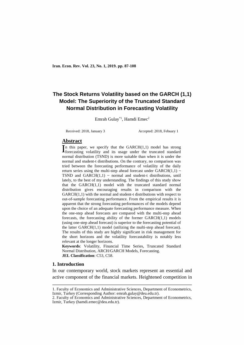
Figure 3: BIST 100 Arithmetic Daily Return Series
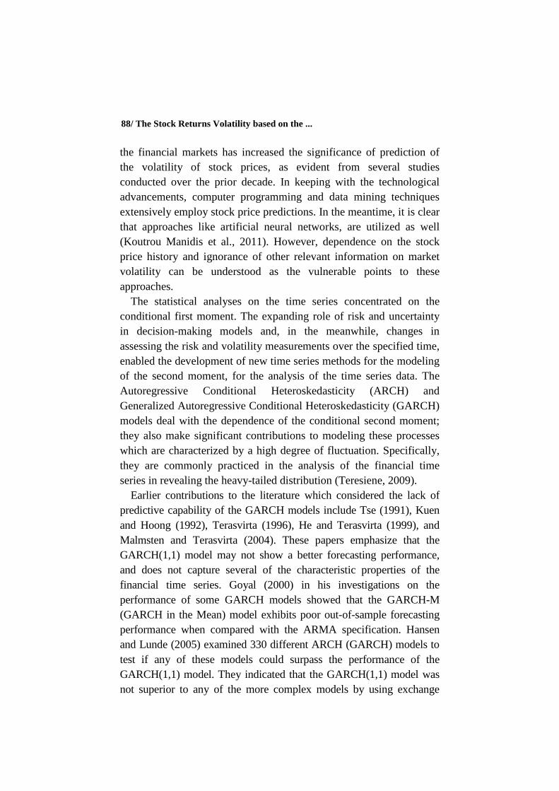
Figure 4: NASDAQ Daily Return Series
The BIST 100 return series are acquired via both logarithmic and
arithmetic average methods. In the greater part of the studies available
in the relevant literature, it is evident that the return series are
calculated using logarithmic formula, whereas the logarithm operation
calculates the return rate for the next year smaller than the return rate
by the arithmetic formula. This situation can be considered as a
different perspective in order to prevent extreme deviations from the
observed values. Therefore, in order to study the performance of a
suggested model when deviated observations are included in the
dataset, the return series were also calculated through arithmetic
formula. Descriptive statistics of the return series of three stocks used
in the application section of the study are summarized in Table 1,
shown below:
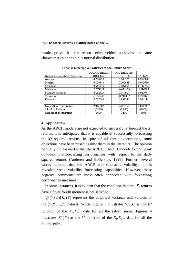
From Table 1 it is clear that the kurtosis of all the return series are
excessive, whereas, the logarithmic and arithmetic BIST 100 return
series exhibited a left-skewed distribution, while the NASDAQ return
series exhibited a right-skewed distribution. In the meantime, all the
return series were observed to not fit the normal distribution. These
0 500 1000 1500 2000 2500 3000 3500-0.1
-0.05
0
0.05
0.1
0 500 1000 1500 2000 2500 3000-0.1
-0.05
0
0.05
0.1
0.15
96/ The Stock Returns Volatility based on the ...
results prove that the return series neither possesses the same
characteristics nor exhibits normal distribution.
Table 1: Descriptive Statistics of the Return Series
4. Application
As the ARCH models are not expected to successfully forecast the 𝑋𝑡
returns, it is anticipated that it is capable of successfully forecasting
the 𝑋𝑡2 squared returns. In spite of all these expectations, some
objections have been raised against them in the literature. The opinion
normally put forward is that the ARCH/GARCH models exhibit weak
out-of-sample-forecasting performances with respect to the daily
squared returns (Anderen and Bollerslev, 1998). Further, several
works reported that the ARCH and stochastic volatility models
revealed weak volatility forecasting capabilities. However, these
negative comments are most often connected with forecasting
performance measures.
In some instances, it is evident that the condition that the tX returns
have a finite fourth moment is not satisfied.
and j j
i iV Y K Y represent the empirical variance and kurtosis of
the 1, ,...,i i jY Y Y dataset. While Figure 5 illustrates 1
kV X as the kth
function of the 1 2, ,..X X data for all the return series, Figures 6
illustrates 1
kK X as the kth function of the 1 2, ,..X X data for all the
return series.

Iran. Econ. Rev. Vol. 23, No.1, 2019 /97
Figure 5: Variance Graphics of the Daily Return Series as the kth Function
Figure 6: The Fourth Moment Graphics of the Daily Return
Series as the kth Function
Figures 5 and 6 show that all the return series would possess a
second finite moment, although they may lack the fourth finite
moment.
According to the graphics obtained for the three return series, their
variances re observed to approach a finite value, but the fourth
moment fails to converge to a finite value. Therefore, the Mean
Absolute Error and Mean Absolute Scaled Error measures are selected
to assess the out-of-sample forecasting performances.
In the next section, first, the parameters of the GARCH(1,1) model
are determined under the assumption that the errors have normal
distribution, student t distribution and TSND distribution. While the
MATLAB software was used for parameter estimations in the
GARCH(1,1) model evaluated under the normal and student-t
distributions, the R-package program was used for parameter
predictions under the TSND distribution.
0 500 1000 1500 2000 2500 3000 3500 40000
1
2
3x 10
-3
NASDAQ
BIST 100 ARITHMETIC
BIST 100 LOGARITHMIC
0 500 1000 1500 2000 2500 3000 3500 40000
2
4
6
8
NASDAQ
BIST 100 ARITHMETIC
BIST 100 LOGARITHMIC
98/ The Stock Returns Volatility based on the ...
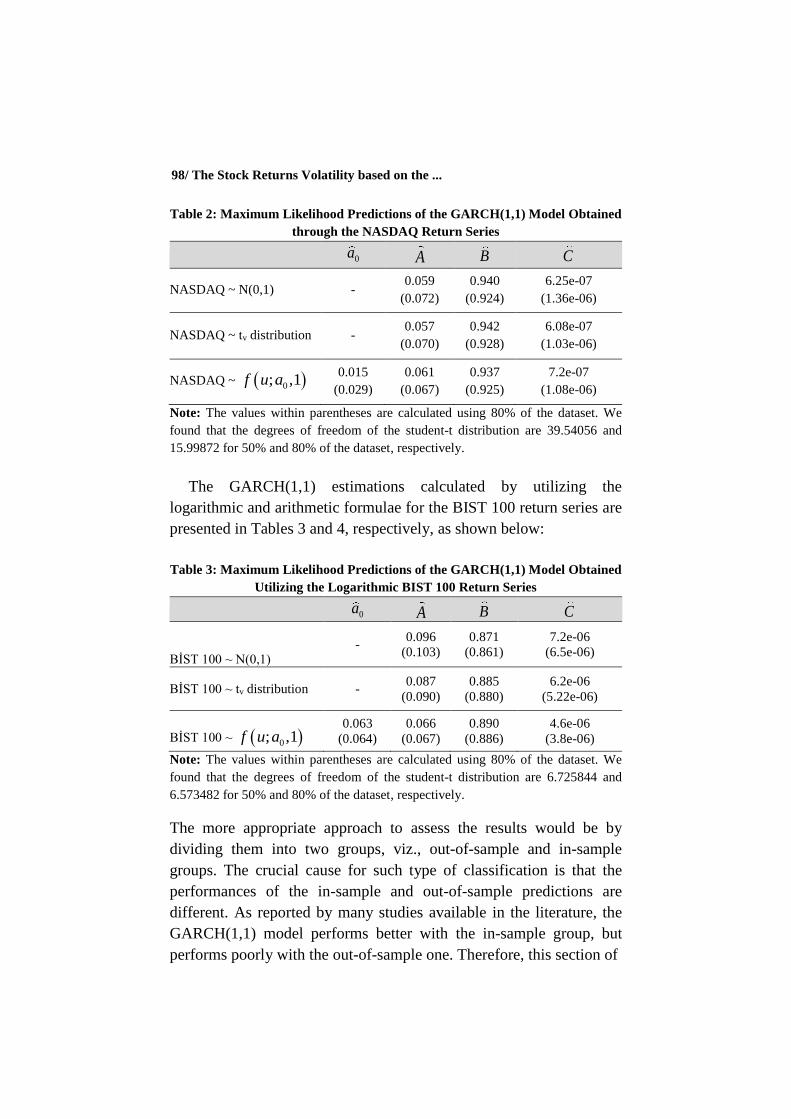
Table 2: Maximum Likelihood Predictions of the GARCH(1,1) Model Obtained
through the NASDAQ Return Series
0a A B C
NASDAQ ~ N(0,1) - 0.059
(0.072)
0.940
(0.924)
6.25e-07
(1.36e-06)
NASDAQ ~ tv distribution - 0.057
(0.070)
0.942
(0.928)
6.08e-07
(1.03e-06)
NASDAQ ~ 0; ,1f u a 0.015
(0.029)
0.061
(0.067)
0.937
(0.925)
7.2e-07
(1.08e-06)
Note: The values within parentheses are calculated using 80% of the dataset. We
found that the degrees of freedom of the student-t distribution are 39.54056 and
15.99872 for 50% and 80% of the dataset, respectively.
The GARCH(1,1) estimations calculated by utilizing the
logarithmic and arithmetic formulae for the BIST 100 return series are
presented in Tables 3 and 4, respectively, as shown below:
Table 3: Maximum Likelihood Predictions of the GARCH(1,1) Model Obtained
Utilizing the Logarithmic BIST 100 Return Series
0a A B C
BİST 100 ~ N(0,1) -
0.096
(0.103)
0.871
(0.861)
7.2e-06
(6.5e-06)
BİST 100 ~ tv distribution - 0.087
(0.090)
0.885
(0.880)
6.2e-06
(5.22e-06)
BİST 100 ~ 0; ,1f u a 0.063
(0.064)
0.066
(0.067)
0.890
(0.886)
4.6e-06
(3.8e-06)
Note: The values within parentheses are calculated using 80% of the dataset. We
found that the degrees of freedom of the student-t distribution are 6.725844 and
6.573482 for 50% and 80% of the dataset, respectively.
The more appropriate approach to assess the results would be by
dividing them into two groups, viz., out-of-sample and in-sample
groups. The crucial cause for such type of classification is that the
performances of the in-sample and out-of-sample predictions are
different. As reported by many studies available in the literature, the
GARCH(1,1) model performs better with the in-sample group, but
performs poorly with the out-of-sample one. Therefore, this section of
Iran. Econ. Rev. Vol. 23, No.1, 2019 /99
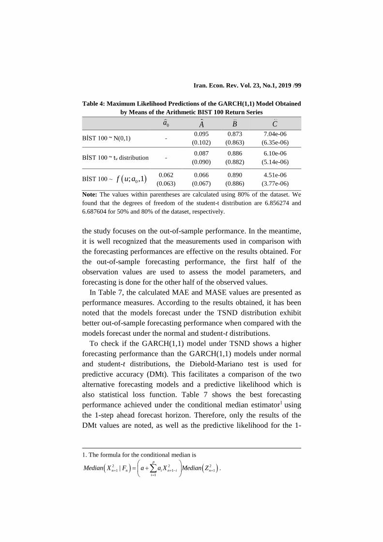
Table 4: Maximum Likelihood Predictions of the GARCH(1,1) Model Obtained
by Means of the Arithmetic BIST 100 Return Series
0a A B C
BİST 100 ~ N(0,1) - 0.095
(0.102)
0.873
(0.863)
7.04e-06
(6.35e-06)
BİST 100 ~ tv distribution - 0.087
(0.090)
0.886
(0.882)
6.10e-06
(5.14e-06)
BİST 100 ~ 0; ,1f u a 0.062
(0.063)
0.066
(0.067)
0.890
(0.886)
4.51e-06
(3.77e-06)
Note: The values within parentheses are calculated using 80% of the dataset. We
found that the degrees of freedom of the student-t distribution are 6.856274 and
6.687604 for 50% and 80% of the dataset, respectively.
the study focuses on the out-of-sample performance. In the meantime,
it is well recognized that the measurements used in comparison with
the forecasting performances are effective on the results obtained. For
the out-of-sample forecasting performance, the first half of the
observation values are used to assess the model parameters, and
forecasting is done for the other half of the observed values.
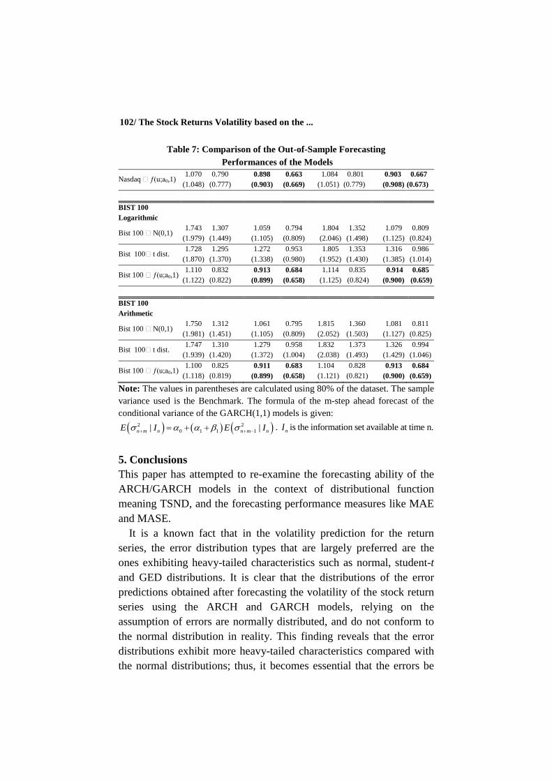
In Table 7, the calculated MAE and MASE values are presented as
performance measures. According to the results obtained, it has been
noted that the models forecast under the TSND distribution exhibit
better out-of-sample forecasting performance when compared with the
models forecast under the normal and student-t distributions.
To check if the GARCH(1,1) model under TSND shows a higher
forecasting performance than the GARCH(1,1) models under normal
and student-t distributions, the Diebold-Mariano test is used for
predictive accuracy (DMt). This facilitates a comparison of the two
alternative forecasting models and a predictive likelihood which is
also statistical loss function. Table 7 shows the best forecasting
performance achieved under the conditional median estimator1 using
the 1-step ahead forecast horizon. Therefore, only the results of the
DMt values are noted, as well as the predictive likelihood for the 1-
1. The formula for the conditional median is
2 2 2
1 1 1
1
|p
n n i n i n
i
Median X F a a X Median Z
.

100/ The Stock Returns Volatility based on the ...
step ahead forecast obtained using a conditional median estimator
(refer Tables 5 and 6).
Therefore, this study has concluded that a statistically significant
difference is present among the forecasting performances of the
GARCH(1,1) models using the TSND distribution, normal and
student-t distributions.
Table 5: The Diebold-Mariano Test for Predictive Accuracy
NASDAQ
DM Test Nasdaq ̴ N(0,1) Nasdaq ̴ t dist.
Nasdaq ̴ ƒ(u;a0,1) 4.52[3.32e-06]
(1.85)[0.03202]
4.59[2.39e-06]
(3.96)[4.21e-05]
BIST 100 Logarithmic
DM Test Bist 100 ̴ N(0,1) Bist 100̴ t dist.
Bist 100 ̴ ƒ(u;a0,1) 5.69[7.49e-09]
(4.26)[1.6e-05]
10.264[2.2e-16]
(7.24)[5.75e-013]
BIST 100 Arithmetic
DM Test Bist 100 ̴ N(0,1) Bist 100̴ t dist.
Bist 100 ̴ ƒ(u;a0,1) 5.75[5.23e-09]
(4.72)[1.40e-06]
10.187[2.2e-16]
(7.65)[3.20e-14]
Note: The null hypothesis is the state when both the methods have the same forecast
accuracy.
For alternative = "greater", the alternative hypothesis shows that method 2 has
greater accuracy than method 1 (GARCH(1,1) ̴ and the TSND model represent
method 2). The values in parentheses are calculated by using 80% of the dataset.
The p-values are enclosed within the square brackets.
Table 6: Negative Predictive Likelihood Results
Conditional Median
NPL
NASDAQ
Nasdaq ̴ N(0,1)
-2.455(-2.508)
Nasdaq ̴ t dist.
-2.406(-2.448)
Nasdaq ̴ ƒ(u;a0,1)
-2.459(-2.526)
BIST 100 Logarithmic
Bist 100 ̴ N(0,1)
-2.528(-2.580)
Bist 100̴ t dist.
-2.448(-2.503)
Bist 100 ̴ ƒ(u;a0,1)
-2.576(-2.608)

Iran. Econ. Rev. Vol. 23, No.1, 2019 /101
Table 6: Negative Predictive Likelihood Results
BIST 100 Arithmetic
Bist 100 ̴ N(0,1)
-2.528(-2.580)
Bist 100̴ t dist.
-2.448(-2.502)
Bist 100 ̴ ƒ(u;a0,1)
-2.578(-2.637)
Note: The values in parentheses are calculated using 80% of the dataset.
The loss of function is to be minimized. The lower the NPL value, The higher the forecasting performance.
Table 7: Comparison of the Out-of-Sample Forecasting
Performances of the Models
1-day ahead forecast 30-days ahead forecast
Conditional
Expectation
Conditional
Median
Conditional
Expectation
Conditional
Median
MAE MASE MAE MASE MAE MASE MAE MASE
NASDAQ
Nasdaq ̴ N(0,1)
1.055
(1.092)
0.780
(0.809)
0.895
(0.903)
0.661
(0.670)
1.076
(1.158)
0.765
(0.859)
0.898
(0.916)
0.664
(0.679)
Nasdaq ̴ t dist. 1.056
(1.106)
0.780
(0.820)
0.913
(0.941)
0.675
(0.698)
1.076
(1.171)
0.795
(0.868)
0.920
(0.965)
0.679
(0.716)
Nasdaq ̴ ƒ(u;a0,1) 1.042
(1.051)
0.770
(0.779)
0.891
(0.898)
0.658
(0.666)
1.055
(1.047)
0.779
(0.776)
0.894
(0.899)
0.660
(0.667)
BIST 100
Logarithmic
Bist 100 ̴ N(0,1)
1.209
(1.258)
0.906
(0.915)
0.912
(0.915)
0.684
(0.670)
1.583
(1.782)
1.186
(1.305)
1.009
(1.046)
0.757
(0.766)
Bist 100̴ t dist. 1.205
(1.236)
0.903
(0.905)
0.992
(1.004)
0.743
(0.736)
1.554
(1.674)
1.165
(1.225)
1.175
(1.227)
0.880
(0.899)
Bist 100 ̴ ƒ(u;a0,1) 1.062
(1.069)
0.780
(0.783)
0.894
(0.888)
0.670
(0.650)
1.094
(1.109)
0.820
(0.812)
0.906
(0.895)
0.679
(0.655)
BIST 100
Arithmetic
Bist 100 ̴ N(0,1) 1.209
(1.257)
0.906
(0.921)
0.913
(0.915)
0.684
(0.670)
1.584
(1.779)
1.187
(1.303)
1.100
(1.045)
0.757
(0.766)
Bist 100̴ t dist. 1.207
(1.244)
0.905
(0.911)
0.992
(1.007)
0.743
(0.737)
1.564
(1.714)
1.172
(1.255)
1.177
(1.245)
0.882
(0.912)
Bist 100 ̴ ƒ(u;a0,1) 1.058
(1.067)
0.793
(0.781)
0.894
(0.888)
0.670
(0.650)
1.086
(1.105)
0.814
(0.810)
0.904
(0.895)
0.678
(0.655)
60-days ahead forecast 90-days ahead forecast
Conditional
Expectation
Conditional
Median
Conditional
Expectation
Conditional
Median
MAE MASE MAE MASE MAE MASE MAE MASE
NASDAQ
Nasdaq ̴ N(0,1)
1.098
(1.227)
0.811
(0.909)
0.902
(0.932)
0.667
(0.691)
1.121
(1.292)
0.828
(0.826)
0.908
(0.951)
0.671
(0.691)
Nasdaq ̴ t dist. 1.097
(1.241)
0.810
(0.920)
0.927
(0.994)
0.685
(0.737)
1.118
(1.311)
0.826
(0.972)
0.936
(1.024)
0.691
(0.758)
102/ The Stock Returns Volatility based on the ...
Table 7: Comparison of the Out-of-Sample Forecasting
Performances of the Models
Nasdaq ̴ ƒ(u;a0,1) 1.070
(1.048)
0.790
(0.777)
0.898
(0.903)
0.663
(0.669)
1.084
(1.051)
0.801
(0.779)
0.903
(0.908)
0.667
(0.673)
BIST 100
Logarithmic
Bist 100 ̴ N(0,1)
1.743
(1.979)
1.307
(1.449)
1.059
(1.105)
0.794
(0.809)
1.804
(2.046)
1.352
(1.498)
1.079
(1.125)
0.809
(0.824)
Bist 100̴ t dist. 1.728
(1.870)
1.295
(1.370)
1.272
(1.338)
0.953
(0.980)
1.805
(1.952)
1.353
(1.430)
1.316
(1.385)
0.986
(1.014)
Bist 100 ̴ ƒ(u;a0,1) 1.110
(1.122)
0.832
(0.822)
0.913
(0.899)
0.684
(0.658)
1.114
(1.125)
0.835
(0.824)
0.914
(0.900)
0.685
(0.659)
BIST 100
Arithmetic
Bist 100 ̴ N(0,1) 1.750
(1.981)
1.312
(1.451)
1.061
(1.105)
0.795
(0.809)
1.815
(2.052)
1.360
(1.503)
1.081
(1.127)
0.811
(0.825)
Bist 100̴ t dist. 1.747
(1.939)
1.310
(1.420)
1.279
(1.372)
0.958
(1.004)
1.832
(2.038)
1.373
(1.493)
1.326
(1.429)
0.994
(1.046)
Bist 100 ̴ ƒ(u;a0,1) 1.100
(1.118)
0.825
(0.819)
0.911
(0.899)
0.683
(0.658)
1.104
(1.121)
0.828
(0.821)
0.913
(0.900)
0.684
(0.659)
Note: The values in parentheses are calculated using 80% of the dataset. The sample
variance used is the Benchmark. The formula of the m-step ahead forecast of the
conditional variance of the GARCH(1,1) models is given:
2 2
0 1 1 1| |n m n n m nE I E I . nI is the information set available at time n.
5. Conclusions
This paper has attempted to re-examine the forecasting ability of the
ARCH/GARCH models in the context of distributional function
meaning TSND, and the forecasting performance measures like MAE
and MASE.
It is a known fact that in the volatility prediction for the return
series, the error distribution types that are largely preferred are the
ones exhibiting heavy-tailed characteristics such as normal, student-t
and GED distributions. It is clear that the distributions of the error
predictions obtained after forecasting the volatility of the stock return
series using the ARCH and GARCH models, relying on the
assumption of errors are normally distributed, and do not conform to
the normal distribution in reality. This finding reveals that the error
distributions exhibit more heavy-tailed characteristics compared with
the normal distributions; thus, it becomes essential that the errors be

Iran. Econ. Rev. Vol. 23, No.1, 2019 /103
considered under different distributions which display heavy-tailed
characteristics while modeling the volatility of the return series.
While selecting the distributions having heavy-tailed characteristics,
the basic difficulty lies in determining the degree of freedom.
Therefore, the selection of the degree of freedom for distributions with
heavy-tailed characteristics arbitrarily necessitates considering a
model that exhibits more heavy-tailed characteristics compared with
the normal distribution in volatility, modeling of the stock return
series and evaluation of out-of-sample forecasting performances.
Further, this distribution, which does not demand arbitrary degree-of-
freedom, and which demonstrates better performance compared with
the normal distribution, and which has at least the same or better
performance compared with the student-t distribution, is termed as
TSND distribution. The distribution shape parameter is denoted by a0.
This parameter is predicted using the pseudo-likelihood method. This
result reveals that parameter selection is not arbitrary.
In order to prove that the forecasting performance of the
GARCH(1,1) model is better under the TSND distribution compared
with the forecasts under normal and student-t distributions, both the
NASDAQ and BIST 100 return series calculated by logarithmic and
arithmetic formulas were used. All the three return series reveal
different characteristics and include different observation numbers. On
the contrary, the studies which report the weak forecasting
performance of the GARCH(1,1) model recognize that when good
forecasting performance measures like MAE and MASE are used, an
acceptable out-of-sample forecasting performance is exhibited. In the
case where the return series lacks a finite fourth moment, the selection
of the MAE or MASE measure, frequently used in the literature, is
correct in terms of the squared returns.
While it has been observed that the forecasting accuracy of
GARCH(1,1)~TSND model, suggested in terms of out-of-sample
performance, is superior to the forecasting accuracy of GARCH(1,1)
model using normal and student-t distributions. Another significant
fact is that the absence of any difference between the forecasting
volatility of the return series calculated by logarithmic or arithmetic
formula. As the coefficient estimations obtained are similar or very
104/ The Stock Returns Volatility based on the ...
close to each other, no difference in terms of out-of-sample
forecasting performances is observed.
The TSND distribution shape parameter displays similarities to the
tv-distribution with v degree of freedom, according to the different
values of a0. For instance, when a0 = 0.1, the TSND distribution
reveals a distribution very close to the t-distribution with 5 degrees of
freedom. However, it is noted that the distribution tail shows slightly
thinner tail characteristics with respect to the t5-distribution. At the
interpretation stage of the results obtained, in order to avoid any
biased assessment, the degree of freedom of the t-distribution is
determined by the MATLAB software, used in the estimation of the
model coefficient.
Several studies in the literature have reported that the resulting
forecasting performances will be effective if the dataset is
distinguished into two sections when out-of-sample forecasting
performances are assessed; while the first section is used to estimate
the parameters of the models, the second section is considered to
determine the forecasting performance. Only half of the dataset is
used for forecasting. However, because the characteristics of the
datasets considered do not bear any of the characteristics of the real
dataset, in the second stage 80% of the dataset is considered while the
remaining 20% is used for forecasting. The findings obtained imply
that by increasing number of observations in the dataset, otherwise
referred to as the training set, and using them in the estimation
parameters of the models, induces a rise in the MAE and MASE
values used in the estimation of the forecasting performances, thus
facilitating the acquisition of the results that concur with the results in
the literature. In the meantime, the occurrence of a rise in the MAE
values was determined for 20% of the dataset forecasted, based on the
coefficients estimated, by considering 80% of the dataset for both the
GARCH(1,1)~ND and the GARCH(1,1)~tv models. These results
reveal that the GARCH models exhibit an excellent out-of-sample
forecasting performance when the fitting forecasting performance
measure is used.
The main thrust is that researchers or practitioners must exhibit
great care when determining the sample size for the training set. They
need to select a reasonable forecasting performance measure and

Iran. Econ. Rev. Vol. 23, No.1, 2019 /105
utilize one model under several distributions to forecast the volatility
present in different datasets.
References
Andersen, T. G., & Bollerslev, T. (1998). Answering the Skeptics:
Yes, Standard Volatility Models Do Provide Accurate Forecasts.
International Economic Review, 39(4), 885-905.
Baillie, R. T., & Bollerslev, T. (1991). Intra-day and Inter-market
Volatility in Foreign Exchange Rates. The Review of Economic
Studies, 58(3), 565-585.
Beine, M., Laurent, S., & Lecourt, C. (2002). Accounting for
Conditional Leptokurtosis and Closing Days Effects in FIGARCH
Models of Daily Exchange Rates. Applied Financial Economics,
12(8), 589-600.
Blattberg, R., & Gonedes, N. (1974). A Comparison of the Stable and
Student Distributions as Statistical Models for Stock Prices. Journal of
Business, 47(2), 244-280.
Bollerslev, T. (1986). Generalized Autoregressive Conditional
Heteroskedasticity. Journal of Econometrics, 31(3), 307-327.
---------- (1987). A Conditional Heteroskedastic Time Series Model
for Speculative Price and Rate of Return. Review of Economics and
Statistics, 69(3), 542-547.
Christodoulakis, G. A., & Satchell, S. E. (1998). Forecasting (Log)
Volatility Models. Discussion Paper in Economics, Retrieved from
https://ideas.repec.org/p/exe/wpaper/9814.html#download.
---------- (2005). Forecast Evaluation in the Presence of Unobserved
Volatility. Econometrics Reviews, 23(3), 175-198.
Engle, R. F. (1982). Autoregressive Conditional Heteroscedasticity
with Estimates of the Variance of United Kingdom Inflation.
Econometrica, 50(4), 987-1007.

106/ The Stock Returns Volatility based on the ...
Garcia, R. C., Contreras, J., Van Akkeren, M., & Garcia, J. B. C. (2005).
A GARCH Forecasting Model to Predict Day-ahead Electricity Prices.
IEEE Transactions on Power Systems, 20(2), 867-874.
Goyal, A. (2000). Predictability of Stock Return Volatility from
GARCH Models. Working Paper, Retrieved from
http://www.hec.unil.ch/agoyal/docs/garch.pdf.
Granger, C. W. J., & Ding, Z. (1995). Some Properties of Absolute
Return: An Alternative Measure of Risk. Annales d'Economie et de
Statistique, 40, 67-91.
Hansen, P. R., & Lunde, A. (2005). A Forecast Comparison of
Volatility Models: Does Anything Beat a GARCH (1, 1)? Journal of
Applied Econometrics, 20(7), 873-889.
He, C., & Terasvirta, T. (1999). Properties of Moments of a Family of
GARCH Processes. Journal of Econometrics, 92(1), 173-192.
---------- (1999). Properties of the Autocorrelation Function of
Squared Observations for Second‐order GARCH Processes Under
Two Sets of Parameter Constraints. Journal of Time Series Analysis,
20(1), 23-30.
Heracleous, M. S. (2007). Sample Kurtosis, GARCH-t and the
Degrees of Freedom Issue. Working Papers, 60, Retrieved from
https://ideas.repec.org/p/eui/euiwps/eco2007-60.html.
Hsieh, D. A. (1989). Modeling Heteroscedasticity in Daily Foreign-
Exchange Rates. Journal of Business & Economic Statistics, 7(3),
307-317.
Javed, F., & Mantalos, P. (2013). GARCH-type Models and
Performance of Information Criteria. Communications in Statistics-
Simulation and Computation, 42(8), 1917-1933.
Kaiser, T. (1996). One-Factor-GARCH Models for German Stocks-
Estimation and Forecasting. Working Paper, 87, Retrieved from
https://papers.ssrn.com/sol3/papers.cfm?abstract_id=1063.

Iran. Econ. Rev. Vol. 23, No.1, 2019 /107
Koksal, B. (2009). A Comparison of Conditional Volatility Estimators
for the ISE National 100 Index Returns. Journal of Economics and
Social Research, 11(2), 1-28.
Koutroumanidis, T., Ioannou, K., & Zafeiriou, E. (2011). Forecasting
Bank Stock Market Prices with a Hybrid Method: the Case of Alpha
Bank. Journal of Business Economics and Management, 12(1), 144-163.
Kuen, T. Y., & Hoong, T. S. (1992). Forecasting Volatility in the
Singapore Stock Market. Asia Pacific Journal of Management, 9(1),
1-13.
Malmsten, H., & Terasvirta, T. (2004). Stylized Facts of Financial
Time Series and Three Popular Models of Volatility. SSE/EFI
Working Paper Series, Retrieved from
http://www.ejpam.com/index.php/ejpam/article/view/801.
Mikosch, T., & Starica, C. (1998). Change of Structure in Financial
Time Series, Long Range Dependence and the GARCH Model.
Working Paper, Retrieved from
http://www.math.chalmers.se/Math/Research/Preprints/1998/60.pdf.
McFarland, J. W., Pettit, R. R., & Sung, S. K. (1982). The Distribution
of Foreign Exchange Price Changes: Trading Day Effects and Risk
Measurement. The Journal of Finance, 37(3), 693-715.
McNeil, A. J., & Frey, R. (2000). Estimation of Tail-related Risk
Measures for Heteroscedastic Financial Time Series: An Extreme
Value Approach. Journal of Empirical Finance, 7(3-4), 271-300.
Politis, D. N. (2004). A Heavy-tailed Distribution for ARCH
Residuals with Application to Volatility Prediction. Annals of
Economics and Finance, 5(2), 283-298.
Poon, S. H., & Granger, C. (2003). Forecasting Financial Market
Volatility: A Review. Journal of Economic Literature, 41(2), 478-539.
Taylor, S. J. (1986). Modelling Financial Time Series. Singapore:
World Scientific Publishing.

108/ The Stock Returns Volatility based on the ...
Terasvirta, T. (1996). Two Stylized Facts and the GARCH (1,1)
Model. Working Paper, Retrieved from
https://www.researchgate.net/publication/5095068_Two_Stylized_Fac
ts_and_the_Garch_11_Model.
Teresiene, D. (2009). Lithuanian Stock Market Analysis Using a Set
of GARCH Models. Journal of Business Economics and Management,
10(4), 349-360.
Tse, Y. K. (1991). Stock Returns Volatility in the Tokyo Stock
Exchange. Japan and the World Economy, 3(3), 285-298.
Vee, D. C., Gonpot, P. N., & Sookia, N. (2011). Forecasting Volatility
of USD/MUR Exchange Rate Using a GARCH (1,1) Model with
GED and Student’st Errors. University of Mauritius Research Journal,
17(1), 1-14.
Vosvrda, M., & Zikes, F. (2004). An Application of the GARCH-t
Model on Central European Sock Returns. Prague Economic Papers,
1, 26-39.
Walenkamp, M. (2008). Forecasting Stock Index Volatility (Master’s
Thesis, Universiteit Leiden, Leiden), Retrieved from
https://www.universiteitleiden.nl/binaries/content/assets/science/mi/sc
ripties/walenkampmaster.pdf.
Yang, M. (2002). Model Selection for GARCH Models Using AIC and
BIC (Master’s Thesis, Dalhousie University, Nova Scotia). Retrieved
from
https://www.researchgate.net/publication/35716946_Model_selection
_for_GARCH_models_using_AIC_and_BIC_microform.
Zivot, E. (2008). Practical Issues in the Analysis of Univariate
GARCH Models. Working Papers, Retrieved from
https://faculty.washington.edu/ezivot/research/practicalgarchfinal.pdf.