Using FunctionUsing Function Lesson 5 © 2014, John Wiley & Sons, Inc.Microsoft Official Academic...
45
Using Function Lesson 5 © 2014, John Wiley & Sons, Inc. Microsoft Official Academic Course, Microsoft Word 2013 1 Microsoft Excel 2013
Transcript of Using FunctionUsing Function Lesson 5 © 2014, John Wiley & Sons, Inc.Microsoft Official Academic...

Using FunctionLesson 5
© 2014, John Wiley & Sons, Inc.
Microsoft Official Academic Course, Microsoft Word 2013
1
Microsoft Excel 2013
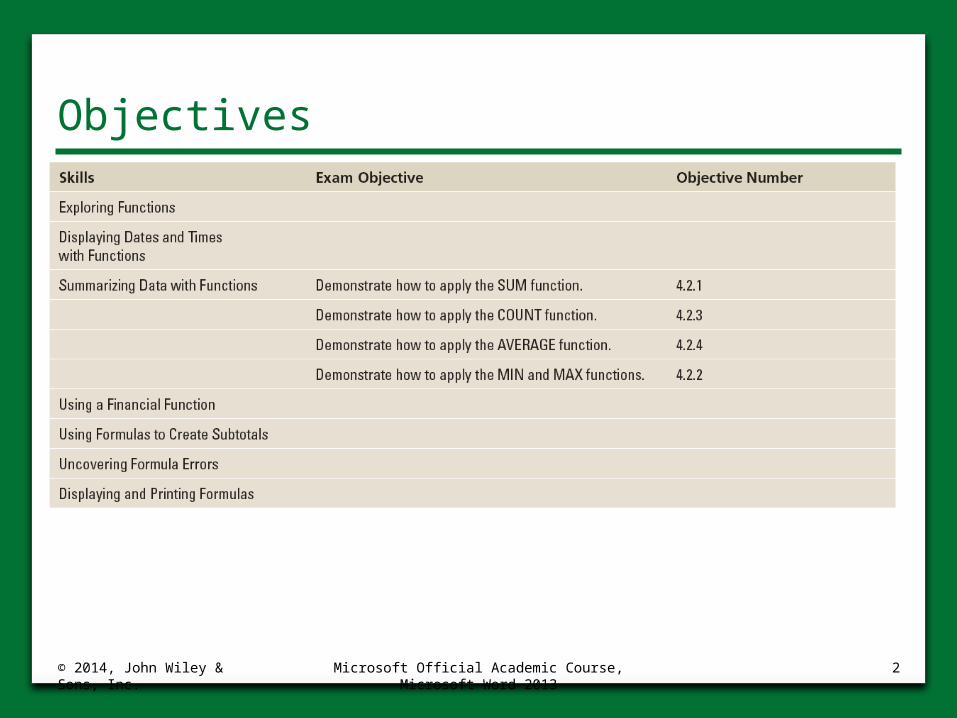
Objectives
© 2014, John Wiley & Sons, Inc.
Microsoft Official Academic Course, Microsoft Word 2013
2
Software Orientation
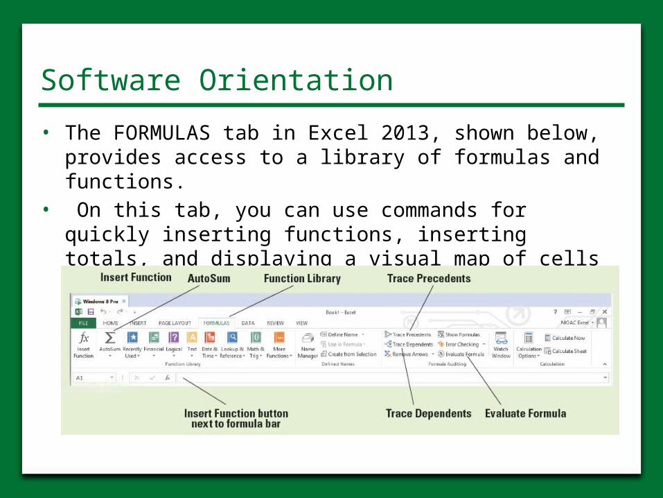
• The FORMULAS tab in Excel 2013, shown below, provides access to a library of formulas and functions.
• On this tab, you can use commands for quickly inserting functions, inserting totals, and displaying a visual map of cells that are dependent on a formula.
Step by Step: Explore Functions
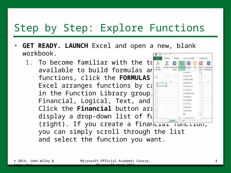
• GET READY. LAUNCH Excel and open a new, blank workbook.1. To become familiar with the tools
available to build formulas and insert functions, click the FORMULAS tab. Excel arranges functions by category in the Function Library group, such as Financial, Logical, Text, and so on. Click the Financial button arrow to display a drop-down list of functions (right). If you create a financial function, you can simply scroll through the list and select the function you want.
© 2014, John Wiley & Sons, Inc.
Microsoft Official Academic Course, Microsoft Word 2013
4
Step by Step: Explore Functions
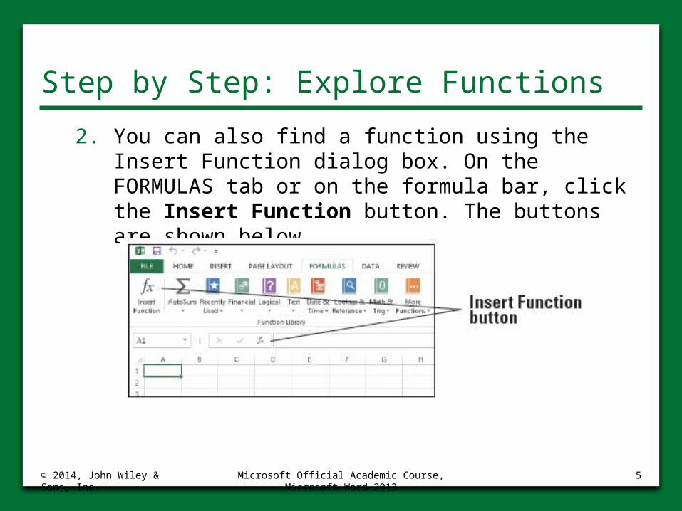
2. You can also find a function using the Insert Function dialog box. On the FORMULAS tab or on the formula bar, click the Insert Function button. The buttons are shown below.
© 2014, John Wiley & Sons, Inc.
Microsoft Official Academic Course, Microsoft Word 2013
5

Step by Step: Explore Functions
3. In the Insert Function dialog box, type a description of what you want to do. For example, type date and click Go. Excel returns a list of functions that most closely match your description (right).
4. With DATE selected in the Select a function list, click OK. The Function Arguments dialog box opens.
© 2014, John Wiley & Sons, Inc.
Microsoft Official Academic Course, Microsoft Word 2013
6
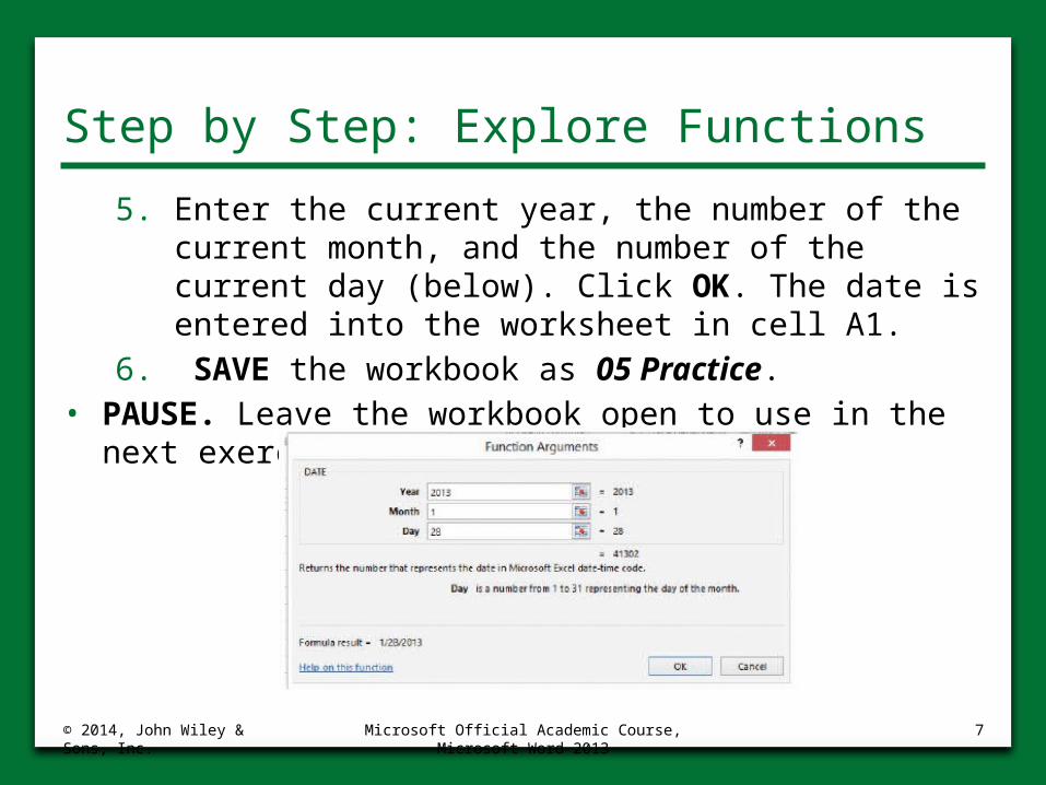
Step by Step: Explore Functions
5. Enter the current year, the number of the current month, and the number of the current day (below). Click OK. The date is entered into the worksheet in cell A1.
6. SAVE the workbook as 05 Practice.• PAUSE. Leave the workbook open to use in the next
exercise.
© 2014, John Wiley & Sons, Inc.
Microsoft Official Academic Course, Microsoft Word 2013
7
Step by Step: Explore Dates
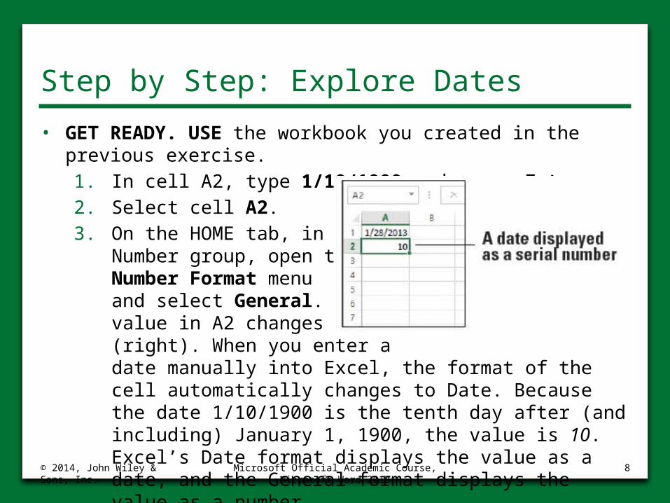
• GET READY. USE the workbook you created in the previous exercise.1. In cell A2, type 1/10/1900 and press Enter. 2. Select cell A2.3. On the HOME tab, in the
Number group, open the Number Format menu and select General. The value in A2 changes to 10 (right). When you enter a date manually into Excel, the format of the cell automatically changes to Date. Because the date 1/10/1900 is the tenth day after (and including) January 1, 1900, the value is 10. Excel’s Date format displays the value as a date, and the General format displays the value as a number.
© 2014, John Wiley & Sons, Inc.
Microsoft Official Academic Course, Microsoft Word 2013
8
Step by Step: Explore Dates
4. With A2 still selected, change the number format to Short Date using the Number Format menu. The cell displays 1/10/1900.
5. In cell A3, type 40000 and press Enter. Because the cell is formatted as General, the value appears as a number.
6. Click cell A2.7. On the HOME tab, in the Clipboard group, click the
Format Painter, and then click cell A3. The formatting of A2 is copied to A3. The value in A3 now appears as a date: 7/6/2009.
8. In cell A4, type =A3-A2 and press Enter. The result is 39990, which is the number of days between the two dates.
9. SAVE the workbook.• PAUSE. Leave the workbook open to use in the next
exercise.
© 2014, John Wiley & Sons, Inc.
Microsoft Official Academic Course, Microsoft Word 2013
9
Step by Step: Use the TODAY Function
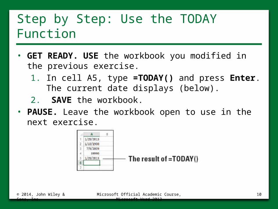
• GET READY. USE the workbook you modified in the previous exercise.1. In cell A5, type =TODAY() and press Enter. The
current date displays (below).2. SAVE the workbook.
• PAUSE. Leave the workbook open to use in the next exercise.
© 2014, John Wiley & Sons, Inc.
Microsoft Official Academic Course, Microsoft Word 2013
10
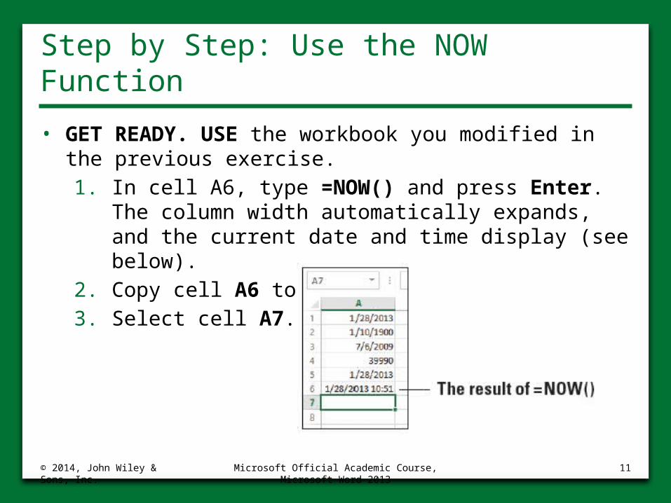
Step by Step: Use the NOW Function
• GET READY. USE the workbook you modified in the previous exercise.1. In cell A6, type =NOW() and press Enter. The
column width automatically expands, and the current date and time display (see below).
2. Copy cell A6 to A7.3. Select cell A7.
© 2014, John Wiley & Sons, Inc.
Microsoft Official Academic Course, Microsoft Word 2013
11
Step by Step: Use the NOW Function
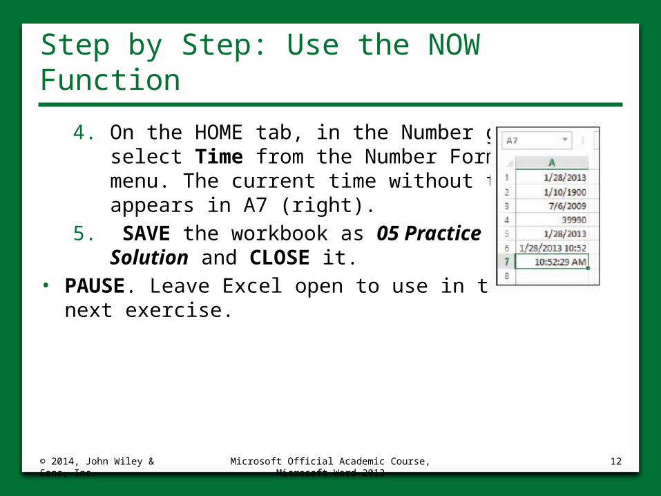
4. On the HOME tab, in the Number group, select Time from the Number Format menu. The current time without the date appears in A7 (right).
5. SAVE the workbook as 05 Practice Solution and CLOSE it.
• PAUSE. Leave Excel open to use in the next exercise.
© 2014, John Wiley & Sons, Inc.
Microsoft Official Academic Course, Microsoft Word 2013
12

Step by Step: Use the SUM Function
• GET READY. LAUNCH Excel if it is not already running.1. OPEN the 05 Budget Start data file for this
lesson. Click Enable Editing, if prompted. This workbook is similar to the 04 Budget workbook created in Lesson 4, but with modifications to accommodate the current lesson.
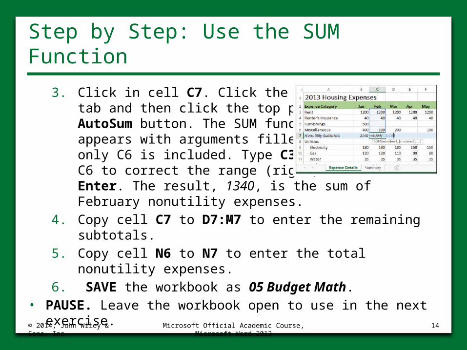
2. In cell B7, type =SUM(B3:B6) and press Enter. The result, 2140, is the sum of January nonutility expenses.
© 2014, John Wiley & Sons, Inc.
Microsoft Official Academic Course, Microsoft Word 2013
13
Step by Step: Use the SUM Function
3. Click in cell C7. Click the FORMULAS tab and then click the top part of the AutoSum button. The SUM function appears with arguments filled in, but only C6 is included. Type C3: before C6 to correct the range (right). Press Enter. The result, 1340, is the sum of February nonutility expenses.
4. Copy cell C7 to D7:M7 to enter the remaining subtotals.
5. Copy cell N6 to N7 to enter the total nonutility expenses.
6. SAVE the workbook as 05 Budget Math.• PAUSE. Leave the workbook open to use in the next
exercise.© 2014, John Wiley & Sons, Inc.
Microsoft Official Academic Course, Microsoft Word 2013
14
Step by Step: Use the COUNT Function
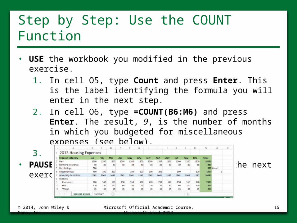
• USE the workbook you modified in the previous exercise.1. In cell O5, type Count and press Enter. This is the
label identifying the formula you will enter in the next step.
2. In cell O6, type =COUNT(B6:M6) and press Enter. The result, 9, is the number of months in which you budgeted for miscellaneous expenses (see below).
3. SAVE the workbook.• PAUSE. Leave the workbook open to use in the next
exercise.
© 2014, John Wiley & Sons, Inc.
Microsoft Official Academic Course, Microsoft Word 2013
15
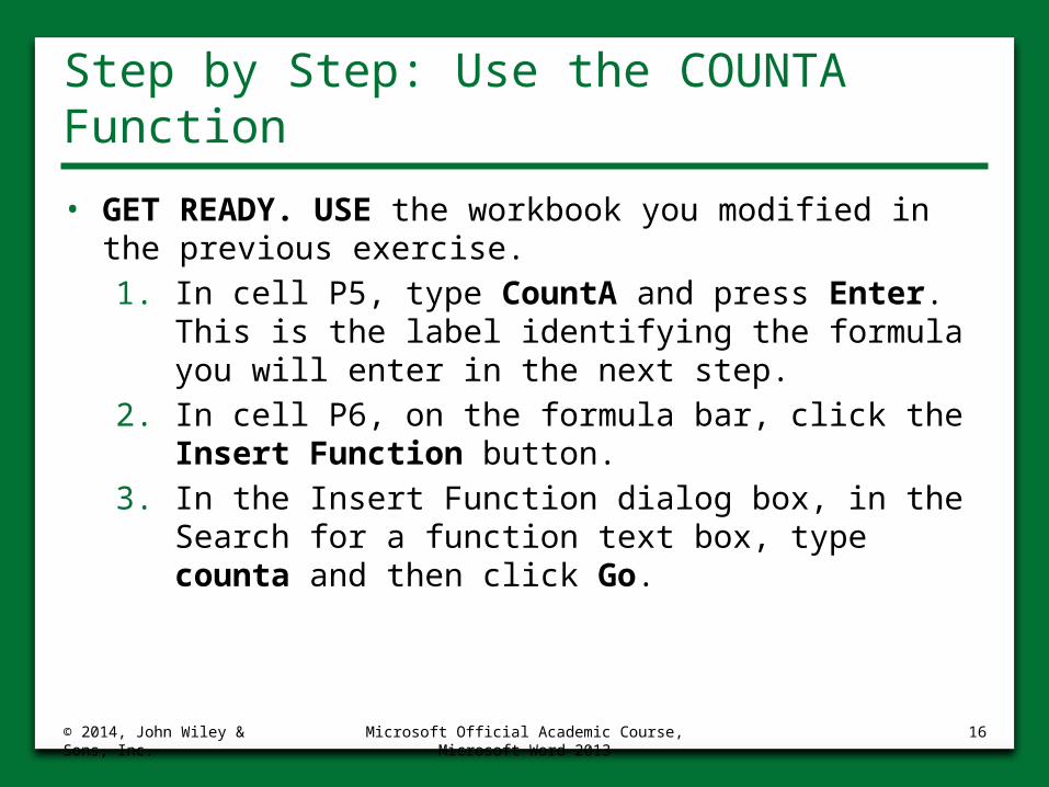
Step by Step: Use the COUNTA Function
• GET READY. USE the workbook you modified in the previous exercise.1. In cell P5, type CountA and press Enter. This is
the label identifying the formula you will enter in the next step.
2. In cell P6, on the formula bar, click the Insert Function button.
3. In the Insert Function dialog box, in the Search for a function text box, type counta and then click Go.
© 2014, John Wiley & Sons, Inc.
Microsoft Official Academic Course, Microsoft Word 2013
16
Step by Step: Use the COUNTA Function
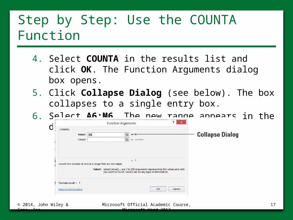
4. Select COUNTA in the results list and click OK. The Function Arguments dialog box opens.
5. Click Collapse Dialog (see below). The box collapses to a single entry box.
6. Select A6:M6. The new range appears in the dialog box.
© 2014, John Wiley & Sons, Inc.
Microsoft Official Academic Course, Microsoft Word 2013
17
Step by Step: Use the COUNTA Function
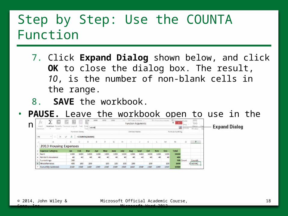
7. Click Expand Dialog shown below, and click OK to close the dialog box. The result, 10, is the number of non-blank cells in the range.
8. SAVE the workbook.• PAUSE. Leave the workbook open to use in the next
exercise.
© 2014, John Wiley & Sons, Inc.
Microsoft Official Academic Course, Microsoft Word 2013
18
Step by Step: Use the AVERAGE Function
• GET READY. USE the workbook you modified in the previous exercise.1. In cell O8, type Average and press Enter. 2. In cell O9, type =AVERAGE(B9:M9) and press
Enter. The result, 175.8333, is your average expected monthly electricity bill.
© 2014, John Wiley & Sons, Inc.
Microsoft Official Academic Course, Microsoft Word 2013
19
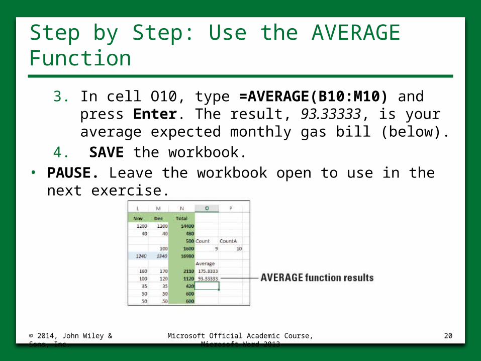
Step by Step: Use the AVERAGE Function
3. In cell O10, type =AVERAGE(B10:M10) and press Enter. The result, 93.33333, is your average expected monthly gas bill (below).
4. SAVE the workbook.• PAUSE. Leave the workbook open to use in the next
exercise.
© 2014, John Wiley & Sons, Inc.
Microsoft Official Academic Course, Microsoft Word 2013
20
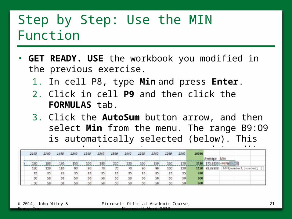
Step by Step: Use the MIN Function
• GET READY. USE the workbook you modified in the previous exercise.1. In cell P8, type Min and press Enter. 2. Click in cell P9 and then click the FORMULAS
tab.3. Click the AutoSum button arrow, and then select
Min from the menu. The range B9:O9 is automatically selected (below). This range is incorrect, so you need to edit it.
© 2014, John Wiley & Sons, Inc.
Microsoft Official Academic Course, Microsoft Word 2013
21
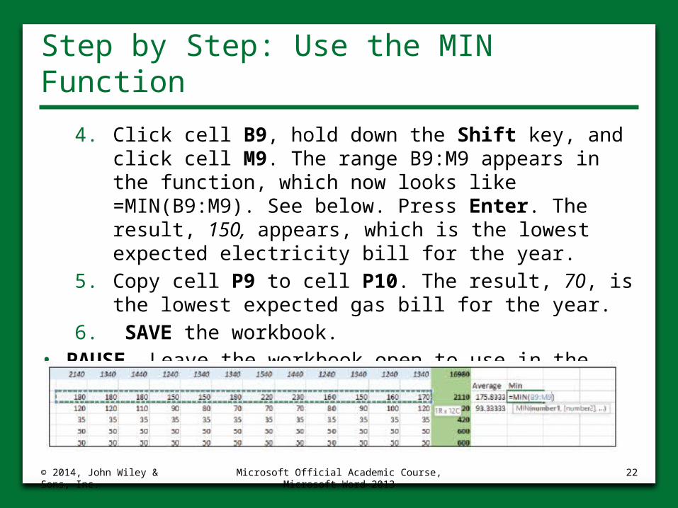
Step by Step: Use the MIN Function
4. Click cell B9, hold down the Shift key, and click cell M9. The range B9:M9 appears in the function, which now looks like =MIN(B9:M9). See below. Press Enter. The result, 150, appears, which is the lowest expected electricity bill for the year.
5. Copy cell P9 to cell P10. The result, 70, is the lowest expected gas bill for the year.
6. SAVE the workbook.• PAUSE. Leave the workbook open to use in the next
exercise.
© 2014, John Wiley & Sons, Inc.
Microsoft Official Academic Course, Microsoft Word 2013
22
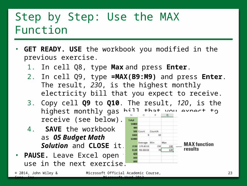
Step by Step: Use the MAX Function
• GET READY. USE the workbook you modified in the previous exercise.1. In cell Q8, type Max and press Enter. 2. In cell Q9, type =MAX(B9:M9) and press Enter. The
result, 230, is the highest monthly electricity bill that you expect to receive.
3. Copy cell Q9 to Q10. The result, 120, is the highest monthly gas bill that you expect to receive (see below).
4. SAVE the workbook as 05 Budget Math Solution and CLOSE it.
• PAUSE. Leave Excel open to use in the next exercise.
© 2014, John Wiley & Sons, Inc.
Microsoft Official Academic Course, Microsoft Word 2013
23
Step by Step: Use the PMT Function
• GET READY. LAUNCH Excel if it is not already running.1. OPEN the 05 Budget PMT data file for this
lesson. 2. In cell R2, type Electronics and press Enter.3. In cell R3, type Interest and press Enter.4. In cell R4, type Years and press Enter.5. In cell R5, type Loan Amt and press Enter.6. In cell R6, type Payment and press Enter.
© 2014, John Wiley & Sons, Inc.
Microsoft Official Academic Course, Microsoft Word 2013
24
Step by Step: Use the PMT Function
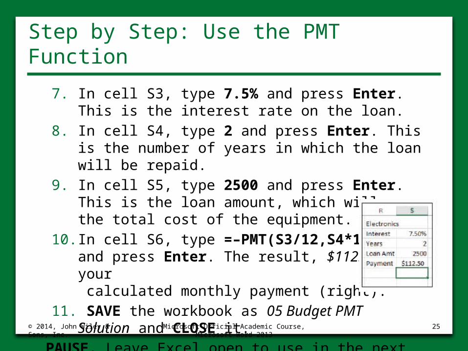
7. In cell S3, type 7.5% and press Enter. This is the interest rate on the loan.
8. In cell S4, type 2 and press Enter. This is the number of years in which the loan will be repaid.
9. In cell S5, type 2500 and press Enter. This is the loan amount, which will cover the total cost of the equipment.
10. In cell S6, type =–PMT(S3/12,S4*12,S5) and press Enter. The result, $112.50, is your calculated monthly payment (right).
11. SAVE the workbook as 05 Budget PMT Solution and CLOSE it.
• PAUSE. Leave Excel open to use in the next exercise.© 2014, John Wiley & Sons, Inc.
Microsoft Official Academic Course, Microsoft Word 2013
25
Step by Step: Select and Create Ranges for Subtotaling
• GET READY. LAUNCH Excel if it is not already running.1. OPEN the 05 Budget Subtotals data file for
this lesson. 2. Select B7:M7.3. On the FORMULAS tab, in the Defined Names
group, click the Define Name button. The New Name dialog box opens.
© 2014, John Wiley & Sons, Inc.
Microsoft Official Academic Course, Microsoft Word 2013
26
Step by Step: Select and Create Ranges for Subtotaling
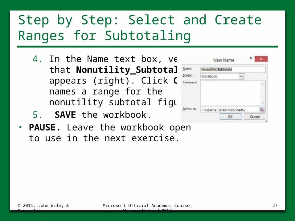
4. In the Name text box, verify that Nonutility_Subtotals appears (right). Click OK. This names a range for thenonutility subtotal figures.
5. SAVE the workbook.• PAUSE. Leave the workbook open
to use in the next exercise.
© 2014, John Wiley & Sons, Inc.
Microsoft Official Academic Course, Microsoft Word 2013
27
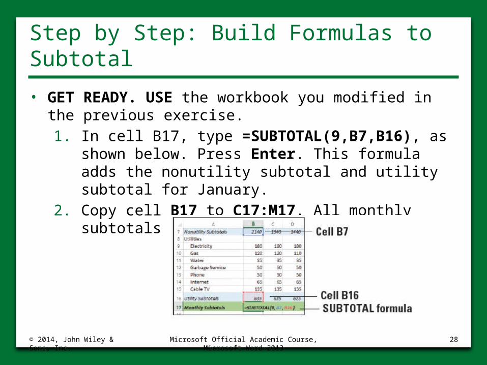
Step by Step: Build Formulas to Subtotal
• GET READY. USE the workbook you modified in the previous exercise.1. In cell B17, type =SUBTOTAL(9,B7,B16), as
shown below. Press Enter. This formula adds the nonutility subtotal and utility subtotal for January.
2. Copy cell B17 to C17:M17. All monthly subtotals are entered.
© 2014, John Wiley & Sons, Inc.
Microsoft Official Academic Course, Microsoft Word 2013
28
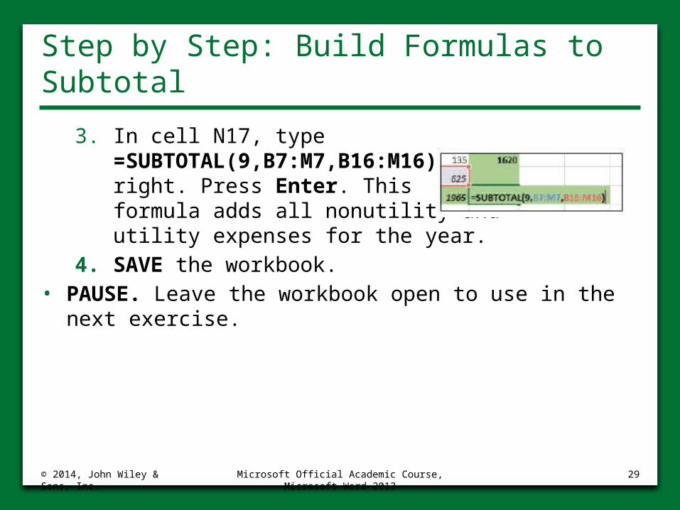
Step by Step: Build Formulas to Subtotal
3. In cell N17, type =SUBTOTAL(9,B7:M7,B16:M16), as shown at right. Press Enter. This formula adds all nonutility and utility expenses for the year.
4. SAVE the workbook.• PAUSE. Leave the workbook open to use in the next
exercise.
© 2014, John Wiley & Sons, Inc.
Microsoft Official Academic Course, Microsoft Word 2013
29
Step by Step: Modify Ranges for Subtotaling
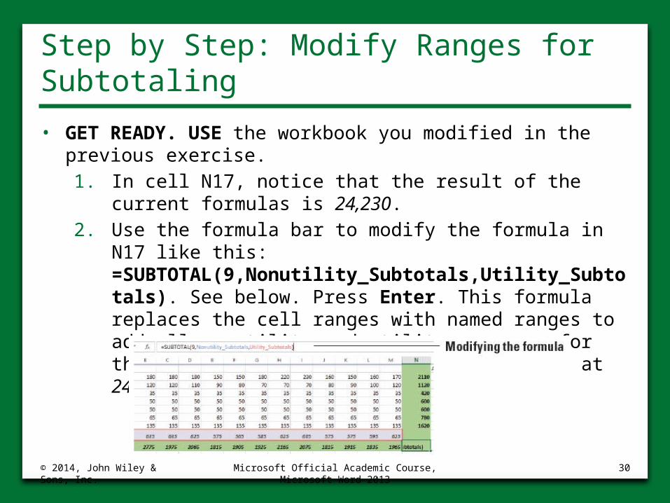
• GET READY. USE the workbook you modified in the previous exercise.1. In cell N17, notice that the result of the current
formulas is 24,230.2. Use the formula bar to modify the formula in N17 like
this: =SUBTOTAL(9,Nonutility_Subtotals,Utility_Subtotals). See below. Press Enter. This formula replaces the cell ranges with named ranges to add all nonutility and utility expenses for the year, and the result remains the same at 24,230.
© 2014, John Wiley & Sons, Inc.
Microsoft Official Academic Course, Microsoft Word 2013
30

Step by Step: Modify Ranges for Subtotaling
3. Click in cell B19 and then click in the formula bar. Change the formula from =SUM(Q1Expenses) to =SUBTOTAL(9,Q1Expenses). This cell sums the named range Q1Expenses. Because the named range includes monthly data and subtotals, you need to correct the range to include only subtotal figures.
4. On the FORMULAS tab, in the Defined Names group, click Name Manager.
© 2014, John Wiley & Sons, Inc.
Microsoft Official Academic Course, Microsoft Word 2013
31
Step by Step: Modify Ranges for Subtotaling
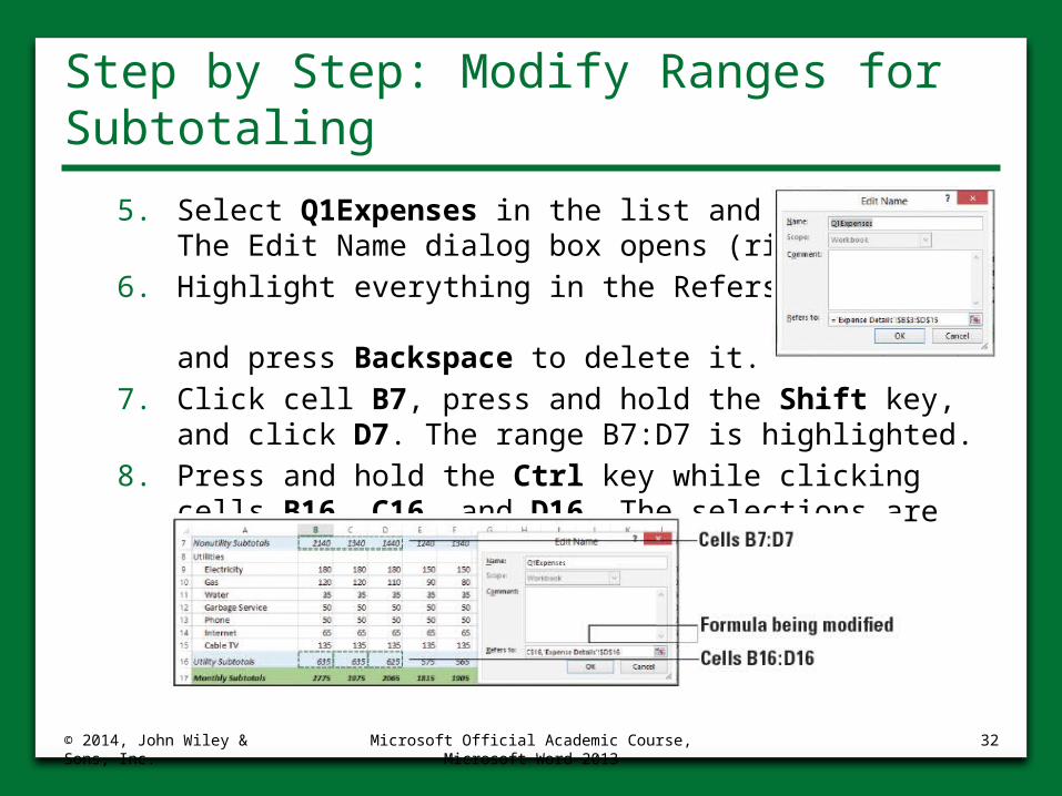
5. Select Q1Expenses in the list and click Edit. The Edit Name dialog box opens (right).
6. Highlight everything in the Refers to text box and press Backspace to delete it.
7. Click cell B7, press and hold the Shift key, and click D7. The range B7:D7 is highlighted.
8. Press and hold the Ctrl key while clicking cells B16, C16, and D16. The selections are shown below.
© 2014, John Wiley & Sons, Inc.
Microsoft Official Academic Course, Microsoft Word 2013
32

Step by Step: Modify Ranges for Subtotaling
9. In the Edit Name dialog box, click OK.10. In the Name Manager dialog box, click Close.11. To verify that you selected the proper ranges for the
Q1Expenses range, open the Name box drop-down list (to the left of the formula bar) and select Q1Expenses. The ranges B7:D7 and B16:D16 are selected (below).
12. Create named ranges for Q2Expenses (E7:G7, E16:G16), Q3Expenses (H7:J7, H16:J16), and Q4Expenses (K7:M7, K16:M16).
© 2014, John Wiley & Sons, Inc.
Microsoft Official Academic Course, Microsoft Word 2013
33
Step by Step: Modify Ranges for Subtotaling
13. Copy the formula from cell B19 to B20:B22. Edit the formulas in cells B20, B21, and B22 to use the appropriate named range. For example, the formula in cell B20 should be =SUBTOTAL(9,Q2Expenses).
14. SAVE the workbook as 05 Budget Subtotals Solution and CLOSE it.
• PAUSE. Leave Excel open to use in the next exercise.
© 2014, John Wiley & Sons, Inc.
Microsoft Official Academic Course, Microsoft Word 2013
34
Step by Step: Review an Error Message
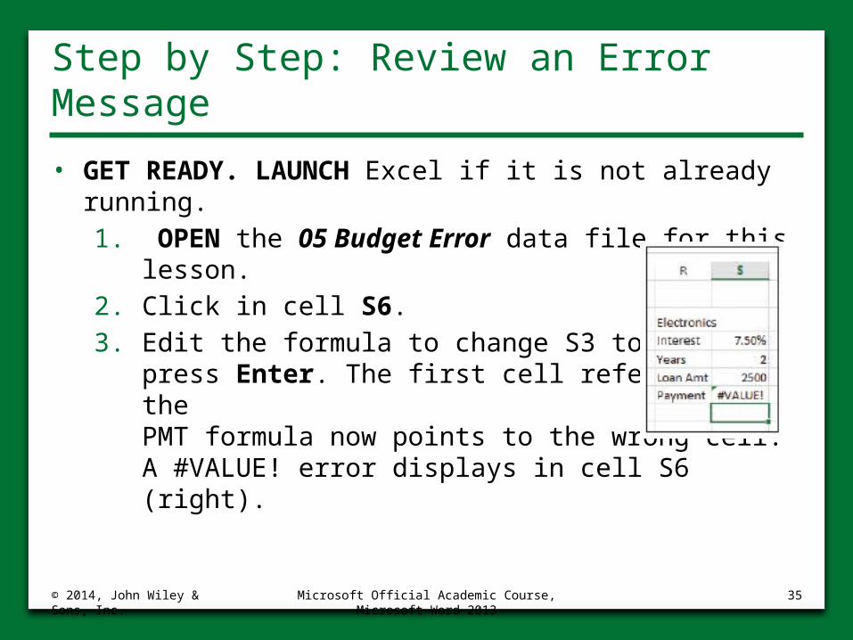
• GET READY. LAUNCH Excel if it is not already running.1. OPEN the 05 Budget Error data file for this
lesson. 2. Click in cell S6.3. Edit the formula to change S3 to R3 and
press Enter. The first cell reference in the PMT formula now points to the wrong cell. A #VALUE! error displays in cell S6 (right).
© 2014, John Wiley & Sons, Inc.
Microsoft Official Academic Course, Microsoft Word 2013
35
Step by Step: Review an Error Message
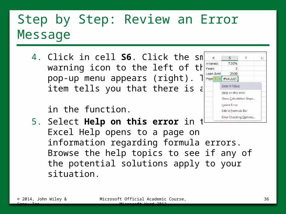
4. Click in cell S6. Click the small, yellow warning icon to the left of the cell. A pop-up menu appears (right). The first item tells you that there is a value error in the function.
5. Select Help on this error in the menu. Excel Help opens to a page on information regarding formula errors. Browse the help topics to see if any of the potential solutions apply to your situation.
© 2014, John Wiley & Sons, Inc.
Microsoft Official Academic Course, Microsoft Word 2013
36
Step by Step: Review an Error Message
6. Close the Excel Help window.7. SAVE the workbook.
• PAUSE. Leave the workbook open to use in the next exercise.
© 2014, John Wiley & Sons, Inc.
Microsoft Official Academic Course, Microsoft Word 2013
37
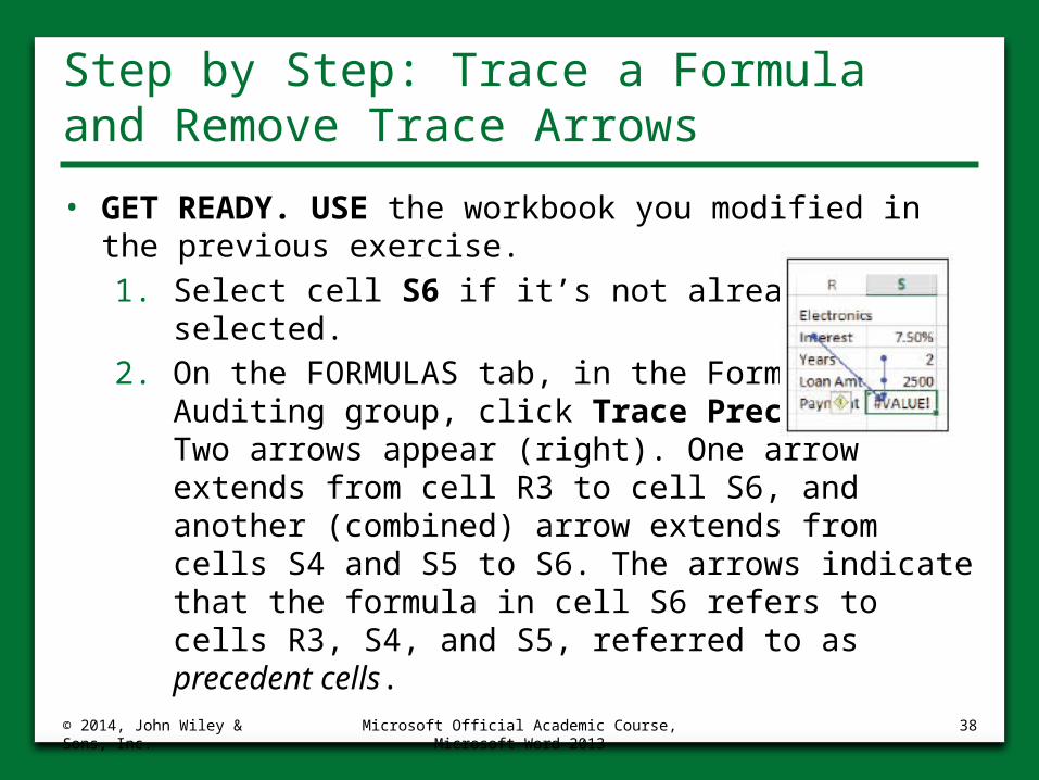
Step by Step: Trace a Formula and Remove Trace Arrows
• GET READY. USE the workbook you modified in the previous exercise.1. Select cell S6 if it’s not already selected.2. On the FORMULAS tab, in the Formula
Auditing group, click Trace Precedents. Two arrows appear (right). One arrow extends from cell R3 to cell S6, and another (combined) arrow extends from cells S4 and S5 to S6. The arrows indicate that the formula in cell S6 refers to cells R3, S4, and S5, referred to as precedent cells.
© 2014, John Wiley & Sons, Inc.
Microsoft Official Academic Course, Microsoft Word 2013
38
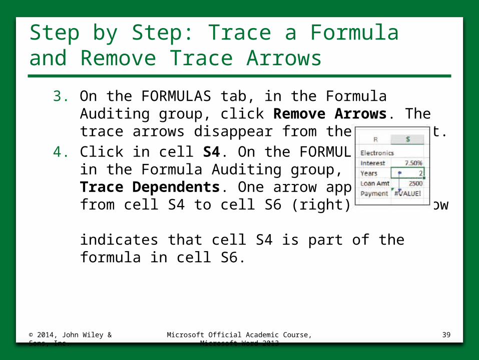
Step by Step: Trace a Formula and Remove Trace Arrows
3. On the FORMULAS tab, in the Formula Auditing group, click Remove Arrows. The trace arrows disappear from the worksheet.
4. Click in cell S4. On the FORMULAS tab, in the Formula Auditing group, click Trace Dependents. One arrow appears from cell S4 to cell S6 (right). The arrow indicates that cell S4 is part of the formula in cell S6.
© 2014, John Wiley & Sons, Inc.
Microsoft Official Academic Course, Microsoft Word 2013
39
Step by Step: Trace a Formula and Remove Trace Arrows
5. SAVE the workbook as 05 Budget Error Solution and CLOSE it.
• PAUSE. Leave Excel open to use in the next exercise.
© 2014, John Wiley & Sons, Inc.
Microsoft Official Academic Course, Microsoft Word 2013
40
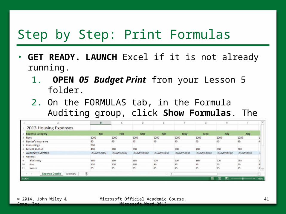
Step by Step: Print Formulas
• GET READY. LAUNCH Excel if it is not already running.1. OPEN 05 Budget Print from your Lesson 5
folder.2. On the FORMULAS tab, in the Formula Auditing
group, click Show Formulas. The formulas appear in the worksheet (below).
© 2014, John Wiley & Sons, Inc.
Microsoft Official Academic Course, Microsoft Word 2013
41
Step by Step: Print Formulas
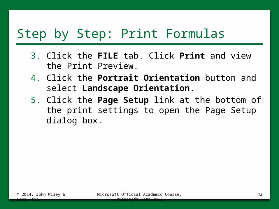
3. Click the FILE tab. Click Print and view the Print Preview.
4. Click the Portrait Orientation button and select Landscape Orientation.
5. Click the Page Setup link at the bottom of the print settings to open the Page Setup dialog box.
© 2014, John Wiley & Sons, Inc.
Microsoft Official Academic Course, Microsoft Word 2013
42
Step by Step: Print Formulas
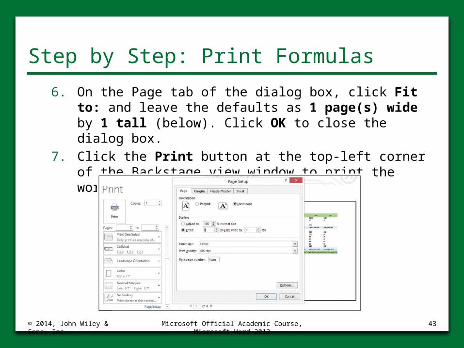
6. On the Page tab of the dialog box, click Fit to: and leave the defaults as 1 page(s) wide by 1 tall (below). Click OK to close the dialog box.
7. Click the Print button at the top-left corner of the Backstage view window to print the worksheet with formulas displayed.
© 2014, John Wiley & Sons, Inc.
Microsoft Official Academic Course, Microsoft Word 2013
43
Step by Step: Print Formulas
8. On the FORMULAS tab, in the Formula Auditing group, click Show Formulas again to stop displaying formulas in the worksheet.
9. SAVE the workbook as 05 Budget Print Solution and CLOSE it.
• CLOSE Excel.
© 2014, John Wiley & Sons, Inc.
Microsoft Official Academic Course, Microsoft Word 2013
44
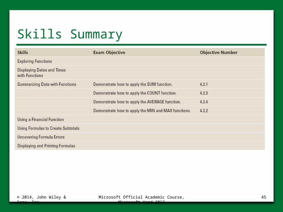
Skills Summary
© 2014, John Wiley & Sons, Inc.
Microsoft Official Academic Course, Microsoft Word 2013
45