NASA Contractor Report 194884

nCP

USING FORMAL SPECIFICATION IN THE GUIDANCE

AND CONTROL SOFTWARE (GCS) EXPERIMENT

Doug Weber and Damir Jamsek

Odyssey Research Associates, Ithaca, NY

Contract NAS1-1897

April, 1994

(NASA-CR-194884) USING FORMAL

SPECIFICATION IN THE GUIDANCE AND

CONTROL SOFT_ARE (GCS) EXPERIMENT.

FORMAL DESIGN AND VERIFICATION

TECHNOLOGY FOR LIFE CRITICAt

SYSTEMS Fina| Report (Odyssey

Research Associates) 114 p G3/60

N94-28267

Unclas

0002421

National Aeronautics and

Space Administration

Langley Research Center

Hampton, VA 23681-0001

https://ntrs.nasa.gov/search.jsp?R=19940023764 2018-07-15T06:52:49+00:00Z

b

Using Formal Specificationin the Guidance and Control Software

(GCS) Experiment

Final Report

Formal Design and Verification Technology

for Life Critical Systems

NASA Contract No. NAS1-18972

ORA Task Assignment 7

Prepared for:

National Aeronautics and Space Administration

Langley Research Center

Hampton, VA 23665

Prepared by:

Odyssey Research Associates, Inc.

301 Dates Drive

Ithaca, NY 14850-1326

4 April 1994

Contents

Overview 1

1.1 Introduction ................................. 1

1.1.1 The Guidance and Control Software ................ 1

1.1.2 ORA's Task ............................. 2

1.2 Formal Methods ............................... 2

1.3 Outline of the Report ............................ 3

2 The Guidance and Control Software

4

4

Formal Methods in DO-178B 22

4.1 The Draft DO-178B Standard ....................... 22

4.2 Including Formal Methods ......................... 23

i

Formal Specification of Control Software 8

3.1 Specifying Software Requirements ..................... 9

3.1.1 Formal Specification ........................ 10

3.2 Control Software Specification ....................... 10

3.2.1 GCS Requirements Analysis .................... 12

3.2.2 GCS Software Requirements .................... 15

3.2.3 Data Fusion ............................. 17

3.2.4 Separating Concerns ........................ 18

3.3 Critique of Informal GCS Requirements Specification .......... 20

5 Summary 24

5.1 Conclusions ................................. 24

5.2 Extensions to this Work .......................... 25

A Formal Specification of GCS 26

A.1 Introduction ................................. 26

A.I.1 Larch ................................ 27

A.1.2 Organization ............................ 30

A.1.3 Terminology and Conventions ................... 32

A.2 Top Level Specification ........................... 33

A.2.1 Basic Sorts ............................. 33

A.2.2 State Machine Specification .................... 34

A.2.3 Communications .......................... 40

A.3 Sensor Processing .............................. 41

A.3.1 Altitude Radar ........................... 42

A.3.2 Accelerometers ........................... 45

A.3.3 Gyroscopes ............................. 48

A.3.4 Touch Down Landing Radar .................... 50

A.3.5 Temperature ............................ 54

A.3.6 Guidance .............................. 56

A.4 Actuator Control .............................. 58

A.4.1 Axial Engines ............................ 59

A.4.2 Roll Engines ............................. 65

A.5 I/O Interface ................................ 69

A.6 Auxiliary Traits ............................... 73

A.6.1 Quads ................................ 74

A.6.2 Rotations .............................. t _

A.6.3 Vectors and Tensors ........................ 78

ii

B

A.7

A.6.4 Integration .............................

GenericTraits ................................

A.7.1

A.7.2

A.7.3

A.7.4

A.7.5

A.7.6

A.7.7

A.7.8

A.7.9

80

80

Polynomials and Polynomial Fitting ................ 81

Sequencesand Histories ...... ................ 84

Linear Equations 86

Arrays and Matrices ........................ 88

Registers............................... 91

Mappings .............................. 92

Statistics ............................... 93

Real Numbers ............................ 94

Natural Numbers .......................... 96

Critique of the Informal GCS Requirements

B.1 GeneralRequirements ...........................

B.2 AECLP ...................................

B.3

B.4

B.5

B.6

B.7

B.8

B.9

B.10

B.11

98

98

99

ARSP .................................... 101

ASP ..................................... 101

CP ...................................... 103

GSP ..................................... 103

GP ...................................... 104

RECLP ................................... 104

TDLRSP ................................... 104

TSP ..................................... 105

Data Dictionary ............................... 107

,°°

in

Chapter 1

Overview

Under the NASA/Langley project titled "Formal Design and Verification Technology

for Life Critical Systems", ORA Corporation is researching better ways to develop

reliable software and hardware. This document is the Final Report for task 7 of that

project. Task 7 is specifically titled "Using Formal Specification in the Guidance and

Control Software Experiment".

1.1 Introduction

1.1.1 The Guidance and Control Software

NASA's Guidance and Control Software (GCS) Experiment is a study of methods for

developing flight control software. The goal of the study is to understand the sources

of software defects, and to find ways to detect and prevent them. In the experiment,

engineers implement GCS several times using various methods: the effect of different

methods can then be compared. [4].

GCS is software to control the descent of a spacecraft onto a planet's surface. The

spacecraft is a simplification of the 1970's Viking Mars lander. By simplifying the

lander, the GCS requirements, design, and code are all shortened, making it possible

to implement GCS several times within the budget of the experiment.

Although simplified, GCS still presents many of the features that characterize con-

trol software. These features will be discussed in the course of the report. Control

software differs in important wavs from other kinds of software, particularly in the

kinds of requirements placed on it. These differences affect the methods engineers use

to develop software; the report will discuss these differences.

1.1.2 ORA's Task

This task has two parts:

1. apply formal methods of software engineering to GCS;

2. understand how formal methods could be incorporated into a software engineering

process for flight control systems.

Both parts of the task are open-ended. There is more than one approach to the

use of formal methods, and within each approach, even partial use of formality can

add to confidence in the software developed. We have begun to apply formal methods

by formally specifying the software requirements for GCS. In the next section we will

explain what this statement means as we introduce the terminology of formal methods.

Defining a good process for developing software is a topic of great current interest.

The aerospace community has already created a standard, DO-178B [3], for software

engineering process. This standard does not determine a specific process, but rather

constrains the possible processes that max' be chosen when developing flight control

software. Software engineers then choose a specific process that satisfies the constraints.

The Do178B standard lists formal methods as an acceptable atlernate means of com-

pliance. A subgoal of our task is to propose a software development process, consistent

with DO-178B, in which formal methods are used.

1.2 Formal Methods

Formal methods bring the precision of mathematical notation, theory, and reasoning to

bear on the problem of understanding the behavior of computer systems. In particular,

a formal specification is a mathematical constraint on a system's intended behavior, and

a formal verification is a mathematical proof that the algorithms used to implement

the system meet the specified constraint. This leads to demonstrably correct systems,

where the assumptions and reasoning on which correctness depends are made explicit.

Formal methods are intended to augment the informal methods conventionally used

in system development. The conventional methods of testing and debugging, when

applied to very complicated systems, have often permitted incorrect, unexpected, or

undependable behavior due to conceptual flaws in design or implementation. This

happens because the informal methods analyze system behavior for particular inputs

only. In contrast, the method of formal verification can apply to all possible inputs,

and so one can analyze at once all the system's possible behaviors.

Formal methods might be applied to any phase of system development, including

requirements analysis, design, implementation of both hardware and software, choice

of test cases, and so forth. In this task we have concentrated on formally specifying

the highest level of software requirements in GCS.

Formal methods can be carried out manually or with the support of automated

tools. Tool support is especially desirable for managing the complexity of verification

proofs. However, in this task we did not carry out any proofs, and our reliance on toolshas been minimal.

1.3 Outline of the Report

In Chapter 9, we describe the lander to be controlled by GCS. The requirements on GCS

are stated in general terms. Our detailed, formal specification of GCS requirements

appears in Appendix A.

In Chapter 3, we discuss the process of requirements analysis for control software

such as GCS. We show that our requirements specification could be improved if more

information were available about the system engineering decisions made in the lander's

design. Specific criticisms of an earlier, informal specification of GCS requirements are

listed in Appendix B.

Chapter 4 relates formal methods to the DO-178B framework. Finally, Chapter 5

draws some conclusions about this work.

Chapter 2

The Guidance and Control

Software

To understand GCS we must understand the lander it is designed to control. In this

chapter we describe the lander. We also describe some key ideas underlying the control

of the lander. The detailed software requirements on GCS can be found by reading the

formal specification of GCS in Appendix A.

The lander is designed to descend through a planetary atmosphere and land safely.

The descent passes through several stages.

• The lander falls, uncontrolled except by parachute, until a predefined altitude is

reached.

• Once that altitude is reached, the engines begin warming up. Active control

begins.

• Once the engines are [lot, the parachute is released. Active control continues.

• After a second predefined altitude near the ground is reached, or the ground is

directly sensed, the engines are shut off and the lander drops to the ground.

The landing is considered safe if the speed is small enough when the engines are shut

off.

The descent has additional properties:

• The altitude measurement depends on GCS, so GCS processing must be started

before reaching the altitude at which the engines are turned on.

altitude

.'*velocity-

speed

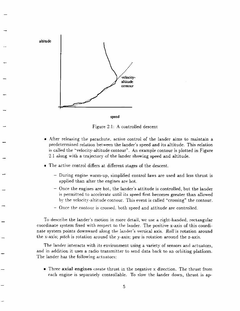
Figure 2.1" A controlled descent

• After releasing the parachute, active control of the lander aims to maintain a

predetermined relation between the lander's speed and its altitude. This relation

is called the "velocity-altitude contour". An example contour is plotted in Figure

2.1 along with a trajectory of the lander showing speed and altitude.

• The active control differs at different stages of the descent.

- During engine warm-up, simplified control laws are used and less thrust is

applied than after the engines are hot.

- Once the engines are hot, the lander's attitude is controlled, but the lander

is permitted to accelerate until its speed first becomes greater than allowed

by the velocity-altitude contour. This event is called "crossing" the contour.

- Once the contour is crossed, both speed and attitude are controlled.

To describe the lander's motion in more detail, we use a right-handed, rectangular

coordinate system fixed with respect to the lander. The positive x-axis of this coordi-

nate system points downward along the lander's vertical axis. Roll is rotation around

the x-axis; pitch is rotation around the y-axis; yaw is rotation around the z-axis.

The lander interacts with its environment using a variety of sensors and actuators,

and in addition it uses a radio transmitter to send data back to an orbiting platform.

The lander has the following actuators:

• Three axial engines create thrust in the negative x direction. The thrust from

each engine is separately controllable. To slow the lander down, thrust is ap-

plied equally from all axial engines. To alter pitch or yaw, torque is supplied by

differences in the thrust from the three engines.

Three opposing pairs of roll engines are mounted on the sides of the lander,

perpendicular to the x-axis. These roll engines provide torque around that axis;

the torque is used to control roll.

A chute release mechanism exists for releasing the parachute.

The lander has the following sensors:

• An altimeter radar measures the lander's altitude by timing the echoes of radar

pulses bounced off the planet's surface.

• Each of three accelerometers measures the lander's acceleration along one co-

ordinate axis.

• Each of three gyroscopes measures the lander's rate of rotation around a coor-

dinate axis.

• Each of four Doppler touch-down landing radars measures the lander's speed

in a single direction. The speed measurements are combined into a measure of

the velocity.

• Two temperature sensors, one solid-state, the other a matched pair of ther-

mocouples, yield a temperature measurement that is used to correct data from

some of the other sensors.

• A touch-down sensor attached to the end of a rod under the lander, detects

when the ground is touched.

Although the lander is a simplified version of the real Viking system, the following

factors are realistic and make GCS's contro,1 task interesting:

• Data from a variety of sensors must be processed.

• Sensor data may be missing or less precise than needed for control, and some

of the lander's physical degrees of freedom cannot be measured directly, so GCS

processing must fuse the sensor data into a precise, coherent model of the lander's

dynamics.

• Control laws must be specified for a variety of the lander's degrees of freedom.

• Some degrees of freedom are affected by several actuators, so the actuators must

be coordinated.

The control laws for the actuators have these goals:

• The roll angle (defined as the integral of the roll rate), is maintained constant.

Controlling roll in this way is desirable for stability so that the control of the

other degrees of freedom does not need to compensate for roll rotation.

• The pitch and yaw angles are controlled so that the lander's x-axis points along

the velocity vector. This ensures that axial engine thrust decreases speed.

• The descent follows the velocity-altitude contour. The contour is (presumably)

chosen to minimize the use of fuel and meet other engineering constraints.

The formal requirements specification in Appendix A gives much more detail about

GCS. The appendix can be read and understood after reading this chapter. The formal

specification is based on a previous informal requirements specification for GCS [7].

That informal specification document contains some helpful illustrations of the lander

and some background references.

The next chapter discusses general problems of specifying requirements, both for-

really and informally. GCS is used as an example.

Chapter 3

Formal Specification of Control

Software

Control software differs from other kinds of software. The difference affects the kinds

of requirements placed on the software, and the process used to decide on those re-

quirements.

Because GCS is control software, we needed to understand this difference before

writing a formal specification of GCS requirements. This chapter presents our analysis.

Control software is special because the purpose underlying it cannot be expressed

without referring to the state of the physical world. The purpose behind GCS, for

example, is to ensure that the lander lands, but does not crash. This purpose has

nothing to do with software, and everything to do with a non-digital, analog reality.

In contrast, the purpose of other kinds of software can often be expressed solely

in terms of digital input and output, or the state of digital devices. The purpose of a

screen editor, for example, is to make the state of the screen a function of the state

of the disk and a history of user commands. In this case, the software designer can

and should make assumptions about the non-digital world that allow that world to be

ignored.

Because the control software cannot ignore the external world, the process of for-

mulating software requirements must be tightly coupled to the engineering decisions

about the system being controlled. We will address the question: What form should

this coupling take?

3.1 Specifying Software Requirements

A requirements analyst should strive to identify and express requirements that have

the following two properties:

1. completeness: every requirement should be stated unambiguously.

2. clarity: only the requirements should be stated, and these should be kept as

simple and as understandable as possible.

Obviously the completeness property is essential for developing reliable software.

Without a complete specification, a programmer must resolve ambiguities in some way,

perhaps by guessing, in order to implement the software. Guessing is not reliable.

The need for clarity is less obvious (judging, at least, by the commonness of massive,

redundant, and overly detailed software requirements documents). Clarity is important

for the following reasons:

Without a clear specification, a programmer is constantly wondering what the

purpose of the software is, and how to extract specific requirements from a lot ofdetail.

• An unclear specification makes it harder for the programmer to see when the

specification itself is in error.

A requirements specification that is unclear because it contains too much detail

is in effect a design document. It is a mistake to mislabel design decisions as

requirements because

m

m

the programmer's freedom to choose the best design is restricted;

when the true requirements are changed, modifying a statement of require-

ments that includes part of the design is harder to do consistently.

Writing a clear requirements specification depends on abstraction. If possible, the

purpose of the software should be stated as the abstract requirement. In the exam-

ple of the screen editor again: "the state of the screen is a function, f, of the state

of the disk and the history of user commands". More detailed requirements can be

shown to imply the abstract requirement. In the screen editor example, the unspecified

function, f, could be refined by giving some of its properties. The process of refining

the abstract requirement into supporting requirements stops when the programmer has

enough information to proceed.

3.1.1 Formal Specification

Formal specification is often touted as a method for writing better requirements. This

claim has merit. Certainly a formal requirements specification is more likely to be

complete than an informal one, because the activity of formalization forces ambiguities

to be addressed.

On the other hand, formal specification does not necessarily help clarity: writing

a overspecification is just as easy in a formal language as in an informal one. Also,

specifiers sometimes find expressing abstract requirements formally to be a problem

because of limitations of a particular formal language.

Most of our discussion will apply both to formal and informal specifications.

3.2 Control Software Specification

When specifying control software, the need for both completeness and clarity creates a

dilemma: should the software requirements be abstract, and in the process describe the

physical svstem being controlled and the environment of that system? Or should the

software requirements be concrete, separating the concerns of the software requirements

analyst from those of the system engineer and physicist?

The clearest software specification would be an abstract statement of the properties

of the controlled system. In the GCS example, "the lander lands without crashing".

However. this specification is not directly a requirement on software; it is quite pos-

sible to satisfy it without any software at all. To produce a complete specification

we must refine this abstract requirement into a collection of concrete requirements the

programmer can work with. as diagrammed in Figure 3.1.

The refinement process, however, is essentially the work of the system engineers who

designed the lander. Reproducing this engineering as part of the software requirements,

using the language of the software requirements, and validating the reasoning behind

each step, could be quite tedious and verbose. Might we just skip this formality and

simply use the collection of concrete requirements as the software specification?

At least one example in the formal methods literature [2] carries out a control

system refinement as part of formally verifying the abstract system requirement. The

example is the control of a vehicle buffeted by crosswind: the control software steers a

straight course even though the environment is unpredictable. This example verifies the

design of the software by proving an abstract requirement about the system, including

the vehicle, the wind, etc. While the example shows that this kind of refinement and

verification is possible, the example is verb' simple, and it is not clear that the approach

it advocates would scale up to larger control systems.

10

systemrequirement

systemcomponent

requirement

softwarerequirement

systemcomponent

requirement

/software

requirement

\Figure 3.1 System requirements analvsis

We contend that this approach is not good, for the following reasons:

The complexity of the system engineering in a control system bears little relation

to the complexity of the software engineering needed to implement the control.

At one extreme, a simple control system might contain a large amount of code;

at the other extreme, a complicated control system might contain only a small

amount of code. In the latter case, demanding that the software requirements

include parts of the system engineering would greatly increase the size of thesoftware task.

The system engineer justifies his work using different kinds of reasoning than the

software engineer. In particular, system engineering typically uses probabilistic

arguments and continuous mathematics, both of which are unusual in the practice

of software engineering. These different kinds of reasoning should be separated.

For complicated environments, simulation often replaces rigorous reasoning as the

primary analysis tool. When simulation is used, the requirements analyst does

not prove that the abstract system requirements are met, but rather offers only

supporting evidence for them. As before, this kind of reasoning should not be

mixed with the reasoning about software requirements.

Generally the system engineering disciplines are better understood than the soft-

ware engineering activities, and so should not be included as part of software

11

engineering. The software engineering task should not be broadened to include

system engineering as well; it is hard enough by itself. Software engineers should

consider using formal methods to improve software, not to try to formalize fields

of engineering that are relatively well understood.

An approach that separates system engineering concerns from software engineering

would be better. This approach recognizes that different people, with different special-

ties and different tools will be responsible for different kinds of engineering. The result

is a hierarchical decomposition of the requirements analysis, as in Figure 3.1.

Unfortunately, the approach we advocate means that the software requirements for

control software will tend to be relatively concrete. They will not state the abstract

goal of the software. If taken in isolation, without the requirements analysis for the

system, they will appear ad hoc.

We advocate an approach in which the software requirements are as abstract as

possible given the condition that they do not describe the physical system being con-trolled. In the next section we use the example of GCS to see what this approach

means.

3.2.1 GCS Requirements Analysis

Let us use the GCS lander as an example to see the kinds of engineering decisions

that must be made in a specific control system before the software requirements can be

stated. In later sections, we will extract from this requirements analysis those features

that will be shared by most or all control systems.

Note that this refinement could be done in more than one way. No documents

describing the lander's requirements analysis were available to us, so some of the re-

finement steps are speculative.

Level 0

At the most abstract level, we simply require that the lander lands without crashing.

This requirement cannot be guaranteed in its current form, because nothing has

been stated about the lander's environment. We must make assumptions about the

environment before the system engineering can begin. For example, we assume that

the winds encountered by the lander do not blow too strongly. Many other assumptions

about the environment are needed.

Even assumptions in this form cannot be certain. Generally we can only claim that

the environment violates our assumptions with some acceptably small probability. We

12

may need to assume a probability distribution for some environmental factors.

Level 1

The first step in refining the level 0 requirement might be as follows. Decide on some

dynamical properties of the lander, such as its mass and fuel supply. Find a set of

trajectories of the lander that satisfy the level 0 requirement without running out offuel.

A trajectory is a path in an abstract space of configurations, where each configuration

tells everything we need to know about the lander's dynamical state. For example, the

configuration will include the lander's altitude and velocity. It may also include other

physical quantities.

In the GCS experiment, the set of trajectories is defined by the velocity-altitude

contour, which is a relation between the lander's speed and altitude. A trajectory is

in the set if it is acceptably close to the velocity-altitude contour. The meaning of

"acceptably close" is not defined in the GC$ documentation; if written out, however,

it would be a definition of distance in the configuration space, with either an upperbound on distance, or a constraint on the distribution of distances.

Figure 2.1 shows one acceptable trajectory for GCS.

The velocity-altitude contour might be gotten in any of several ways. Perhaps

it is derived analytically, possibly using the variational calculus and minimizing the

lander's fuel consumption. Perhaps it is found to be a good choice by using simulation.

Whatever the method, once we define the contour and acceptable deviations from it,

we can (at least in principle) prove that the level 0 requirement is met. The level 1

requirements are sufficient conditions.

A proof of the level 0 requirement depends on the level 0 assumptions about wind,

etc. but also oil new requirements on the lander. For example, we must make new

requirements about the efficiency of the lander's engines for turning fuel into thrust.

These requirements constrain the engines' design.

Level 2

We next refine the level 1 requirement into more specific level 2 requirements on the

lander's design. The level 2 requirements must be sufficient to guarantee the ones atlevel 1.

Level 2 includes the control laws to be enforced. These laws are a mapping from

the lander's configuration to an impulse needed to control the lander. An impulse may

13

be literally a change in momentum (this is the technical meaning of the term) or more

generally some effect produced by the lander's actuators.

Level 2 also includes requirements on the precision with which the control must

be implemented. It also includes an upper bound on delays between the time of ex-

ternal disturbances and the response time of the control. Each of these requirements

constrains the design of the system and its software.

One way to show that the level 2 requirements imply those at level 1 is to construct

an inductive proof. To do this, we show that the lander starts on an acceptable trajec-

tory. We also show that if the lander is following an acceptable trajectory now, then

the level 2 requirements, plus the level 0 assumptions about the environment, plus the

physics of the lander, imply that the lander will continue to follow an acceptable tra-

jectory for some time step in the future. The induction proves that the lander always

follows an acceptable trajectory. The detailed proof might be quite difficult, the time

step might be dependent on the configuration, and it would involve reasoning about

probabilities, but in principle it could be carried out.

Level 3

The level 2 requirements can be refined into level 3 requirements, some of which are

constraints directly on GCS. At this level, we find the requirements that a programmer

needs to begin the task of implementing GCS.

GCS processing is to be implemented as a sequence of frames, each of which pro-

cesses new sensor data, estimates the lander's current configuration, and determines

new outputs to the actuators. We will call the estimate of the configuration a model.

The single step, control, at level 2 has now been refined into three steps: sense, model,

act.

The level 2 requirement on response time is a constraint on the length of each frame.

Level 3 requirements on the software processing time for one frame, together with

specific requirements on the response time of sensors and actuators, plus assumptions

about allowable concurrency between hardware and software, will imply the level 2

requirement.

The level 2 requirement that control laws be implemented is implied by level 3

requirements that the sensor and actuator processing be accurate, and that the model

be accurate.

The level 2 requirement on the precision of the lander's control is implied by a com-

bination of level 3 requirements on precision _. We require that sensors and actuators

"Precision" and "accuracy" are not synonyms. For a definition and discussion of these terms, see

section 3.2.3.

14

be accurately calibrated to a specifiedprecision. We require that the GCS processingmaintain a specifiedprecision.

3.2.2 GCS Software Requirements

The refinement of the lander's requirements in the previous section shows the kind of en-

gineering design decisions we expect would precede a software requirements document.

Following our stated approach, we do not want to include in the software requirements

for GCS any requirement for which the configuration of the lander or the state of the

environment must be described. This leaves the following list of requirements.

a real-time constraint on the length of each frame;

the control laws to be implemented (these map the GCS model, i.e., the estimate

of the lander's configuration, to the impulse needed to control the lander);

an accurate calibration of each sensor (by "calibration" in this case we mean

an algorithm for converting between raw sensor data and a measurement of a

physical quantity);

an accurate calibration of each actuator (by "calibration" in this case we mean

an algorithm for converting between the impulse expected from the actuator and

digital values sent to that actuator);

requirements on the precision of computations;

• a requirement that the model be accurate to a specified precision.

These requirements, though derived for GCS, would apply to most control software.

All bul the last of these requirements can be implemented by the programmer indepen-

dently of concerns about the external world. The last requirement, that the estimate

of the lander's configuration be accurate, may involve facts about the external world,

and for GCS it necessarily does. For this requirement, we have yet to see how software

requirements can be made not to depend on a description of the controlled system.

Figure 3.2 shows the processing taking place in each GCS frame. The solid arrows

represent GCS computation. The dotted arrows represent interaction with the external

world. We have discussed each step in this figure except for "data fusion". In the next

section we will discuss data fusion and its relationship to the requirement on the model

accuracy.

15

configuraUon

¥raw sensor data

calibration

pamal model

model

control

computed impulse

calibration

raw actuator data

previousmodels

¥

impulse

Figure 3.2: Control within one frame

16

sequenceoflander'smodels

abstracdon

3.2.3

sequence oflander'sconfigurations

L.. _1

oneframe

Data Fusion

time

The model computed by GCS is an estimate of the external configuration, and it is an

abstraction: the model reflects those aspects of the lander's dynamics that are needed

for control, while other aspects are ignored. The model is maintained throughout

the lander's descent, during a sequence of frames. The maintenance of the model is

diagrammed in Figure 3.2.3.

To construct the model in each frame, a control system may need to "fuse" data

from different sensors. It may also need to extrapolate from a sequence of models

constructed previously to get a current model, and then "fuse" the extrapolation with

sensor data from the current frame.

Both of these kinds of data fusion occur in GCS. The following cases demonstratethis fact.

Both the altitude and touch-down landing radars may fail to provide raw sensor

data in a particular frame.

If altitude data is missing, GCS extrapolates from previous altitude measure-

ments, making assumptions about the lander's acceleration between frames.

If the extrapolation is not precise enough because previous altitude measure-

ments were also missing, GCS integrates the velocity to yield an estimate ofaltitude.

If one touch-down landing radar value is missing out of four, GCS can still

use the remaining three values to determine the three components of the

lander's velocity; the four radar values are redundant. However, if more than

17

one value is missing, GCS integrates the acceleration to yield an estimate of

velocity.

• GCS judges some acceleration measurements to be unreliable because they are

too far from an extrapolation of recent measurements. In that case, GCS uses

the extrapolation instead of the measurement.

• GCS fuses the temperature measurements from two different sensors to yield a

single value.

In general, the purpose of data fusion in a control system is to construct a better

model. But what do we mean by better?

Accuracy and Precision

In scientific use, the terms accuracy and precision are not synonyms. A textbook

reference [1] defines them:

The accuracy of an experiment is a measure of how close the result of

the experiment comes to the true value. Therefore, it is a measure of the

correctness of the result. The precision of an experiment is a measure of

how exactly the result is determined, without reference to what that result

means. It is also a measure of how reproducible the result is.

The concepts behind these terms are independent: a measurement can be precise but

not accurate, or accurate but not precise.

We can now answer the question from the previous section. Given two models that

are accurate, the better model is the one that is more precise.

3.2.4 Separating Concerns

GCS, like many other software control systems, maintains a model of the external

world. This model is required to be both accurate and precise. Our distinction between

accuracy and precision, though, allows us to separate the concerns of control software

and system engineers.

Maintaining the model's precision is clearly the software engineer's concern. Given

assumptions about the precision of sensors, and knowing the precision of previous

models, the software engineer should be able to determine whether a given data fusion

algorithm maintains the necessary precision for the model. The precision is affected

18

both by the fusing of data with different precisions and by the finite precision of the

computer.

Maintaining accuracy, on the other hand, may involve knowledge of the external

world. Therefore, deciding whether a given data fusion algorithm is accurate becomes

the system, not the software, engineer's problem. For example, underlying some of

the data fusion in GCS is the judgement that the change in the lander's acceleration

between frames is negligible. The control software engineer is not usually able to make

this kind of judgement because it depends on the physics of the system.

Two approaches are possible for developing data fusion algorithms for control soft-

ware, and at the same time specifying the software requirements on data fusion.

The system engineers can simply state the data fusion algorithms as part of the

software requirements. This approach has the advantage of decoupling the system

and software engineering tasks. This is the approach taken to date in the GCS

requirements specification.

The system and software engineers can cooperate to specify a class of accurate

data fusion algorithms, then specify a lower bound on the precision needed from

these algorithms. This approach has the advantages of yielding a more abstract

specification of requirements and therefore allowing the software engineer more

freedom in implementing the software. It has the disadvantage that the specifi-

cations may be more difficult to express formally.

The second approach could have yielded more abstract specifications for several

GCS modules. One example of this increased abstraction arises in processing touch-

down landing radar (TDLR) inputs to yield a velocity measurement.

The data fusion algorithm GCS uses to determine velocity from TDLR clearly does

not maximize precision. To see this, note that if only one touch-down landing radar

vields a value in a particular frame, that value is ignored and integration is used instead

to estimate the lander's velocity. But integration yields a value almost certainly less

precise than the direct radar measurements. So combining the single radar value with

the integration would give greater precision.

Maximizing precision, though, is not the goal of GCS data fusion. The goal is to

satisfy a constraint on precision, along with constraints on the use of time and space by

GCS. Rather than requiring a particular data fusion algorithm for TDLR, one might

have stated the more abstract constraint on precision directlv. Then not only would

the true GCS requirements be clearer, but the GCS programmer might have chosen to

implement a different algorithm, trading off precision for throughput, for example.

Our conclusion is that the GCS software requirements could have been expressed

more clearly and abstractly, while still avoiding any description of the lander or its

19

environment. However, the information about system engineering decisions needed to

state bounds on precision was not available to us. Therefore we were unable to write a

more abstract specification. In the next section we use the analysis of this chapter to

critique the specification of requirements that was available to us.

3.3 Critique of Informal GCS Requirements Spec-

ification

Our formal specification of GCS requirements in Appendix A is based on an earlier,

informal software requirements document [7]. We will refer to the informal software

requirements document as "SR'.

In the process of writing the formal specification we noted some problems with SR.

Understanding most of these problems requires a detailed knowledge of GCS. These

detailed problems are collected into Appendix B.

In this section we ask a more general question: how does the list of requirements in

SR compare to the list in Section 3.2.2 that follows from our analysis? By comparing

and noting differences in these lists, we argue that SR has the following deficiencies as

a requirements specification.

• The requirements on GCS functionality are overspecified. SR specifies function-

alitv for control, for calibrations, and for data fusion, but it goes far beyond what

is needed by specifying intermediate and temporary variables and by telling in

detail how the functionality is to be implemented. This extra detail makes SR

essentially a software design document instead of a requirements specification.

• Thc requirements on GCS timing are overspecified. SR specifies the top-level

timing requirement that each frame must complete within a given time. However,

SR also divides the GCS functionality into modules, puts real-time requirements

on each, and specifies a detailed schedule for executing these modules. The

reasons underlying these extra requirements are not clear from SR. This extra

detail reinforces the impression that SR is essentially a detailed design for GCS.

• The requirements on GCS precision are given too little attention. SR states

upper bounds on precision in the following way: every variable in the design is

listed in a "data dictionary", and a number of bits is specified for each variable.

However, the analysis above shows that it is lower bounds on precision that are

most important in requirements specification.

Our conclusion is that SR does not meet the goals of completeness and clarity advocated

at the beginning of this chapter.

2O

In our formal specification we have attempted to remove as much of SR's overspec-

ification as possible. In general outline, though, our formal specification follows SR.

Because SR does not provide much information about the system design decisions, we

could not attempt to write a more abstract specification using the approach described

in Section 3.2.4.

21

Chapter 4

Formal Methods in DO-178B

A great deal of attention is currently being focussed on the process of software engi-

neering, and proposals for improving it. Some of that attention concerns the use of

formal methods. In this chapter we consider the addition of formal methods to software

engineering practice that follows the D0-178 standard for aircraft systems.

4.1 The Draft DO-178B Standard

The aviation community has produced a standard, DO-178B, which guides the process

of engineering software for airborne systems.

The purpose of DO-178B is, in its own words

...to identify objectives and describe acceptable techniques and methods

for tile development and management of software for airborne digital sys-

tems and equipment. The application of these techniques and methods are

designed to produce software that performs its intended function with a

level of safety that is in compliance with airworthiness requirments and to

provide evidence of compliance with those requirements.

DO-178B does not prescribe a software development method. Rather, it is a guide-

line for deciding on and using acceptable methods. The acceptability of a method for a

particular software component depends on the criticality of that component, i.e., howhazardous would failure of the component be. The more critical the component, the

greater the evidence needed that the component satisfies its requirements.

Planning the software development is a beginning step in any method acceptable un-

der DO-178B. The planning should describe various processes comprising the method.

22

The processes are themselves composed of activities. There are two kinds of processes:

1. Direct processes are those that directly support software development. They

include requirements analysis, design, coding, and integration.

2. Integral processes are those that support the direct processes and are ongoing

throughout the software life-cycle. Examples of integral processes are verification

and configuration management.

4.2 Including Formal Methods

Formal methods may be appropriate in a DO-178B software development plan. Formal

methods encourage a disciplined approach to software development and provide evi-

dence of higher software quality. Both these attributes of formal methods are important

especially for software components that are critical to aircraft safety.

Formal specification, as we have done for GCS requirements, could be an additional

activity in both the requirements analysis and design processes. Based on our GCS

experience, we think the following constraints should be satisfied if formal specification

is used in either process.

• The activities of informal and formal requirements specification (or design speci-

fication) should be combined. The products of these activities should be redun-

dant, differing only in the method of expression, and so combining them should

not create problems.

Some software projects using formal methods have separated the informal activ-

ities from the formal because the latter often take longer and apparently need to

be done by specialists. Separating the activities in this way, however, easily leads

to inconsistencies between the formal and informal specifications, and eventually

to one or the other specification becoming superfluous.

• The activity of requirements analysis for control software should be concurrent

with system requirements analysis. This concurrency allows the software analysts

to discuss their analysis with system engineers in order to learn the rationale and

assumptions behind the requirements imposed on them.

The alternative to this concurrent approach works much like our experience with

GCS: requirements are first placed on the software, and considered finished, with-

out a sufficient explanation of assumptions underlying them. In this situation a

software specifier finds it difficult to express clear, abstract requirements of the

kind discussed in Chapter 3.

23

Chapter 5

Summary

5.1 Conclusions

Writing a formal specif[-lzication of GCS requirements was the central activity of this

task. However. the resulting specification is less important than the lessons we have

learned in writing it. We summarize those lessons as follows.

• Formal requirements specification can be routine.

In their foreword to the informal software requirements document for GCS [7],

Dunham and Withers explain the rationale for their choice of methods:

[GCS] is specified using an extension to the popular method of struc-

tured analysis. This specification method was selected instead of a

formal one for the sole purpose of not making the specification devel-

opment activity a research effort in itself.

This view of formal specification is mistaken. Writing the formal specification of

GCS in Appendix A was straightforward. No research needed to be done. The

specification was written in the Larch language, but many other specification

languages would have worked as well.

Research is needed, however, in the following areas:

- understanding how to write specifications that are both clear and complete,

as defined in chapter 3;

- finding tools that support the analysis of specifications.

Note that these research activities apply both to formal and informal methods,

and therefore should not be considered special obstacles to the use of formal

specification.

24

Control software requirements pose a unique problem for specification.

The problem is in choosing the right level of detail for the specification. Our

analysis of this problem in Chapter 3 can be summarized this way: the specifi-

cation must be detailed enough to be complete, yet abstract enough to be clear.

When specifying a control system, abstraction naturally leads to specifications

of the system being controlled and to assumptions about its environment; these

are outside the domain of software engineering. In Chapter 3, we argue that

a balance must be struck between completeness and abstraction. We also argue

that if more detail about the system engineering behind the GCS lander had been

available, we could have written our formal specification more clearly while still

avoiding descriptions of the lander and its environment.

Formal methods can be used to augment current software development

processes.

Chapter 4 explains how formal specification could be incorporated into DO-178B,

and lists some constraints on software development processes using formality.

5.2 Extensions to this Work

The natural steps to take after specifying a system's requirements are implementing

and verifying that system. If GCS were implemented in Ada, a Larch/Ada interface

specification could easily be written from the specification in Appendix A. The leading

software tool for verifying Larch/Ada specifications is ORA's Penelope environment

[,5].

25

Appendix A

Formal Specification of GCS

A.1 Introduction

This chapter contains the formal requirements specification for NASA's Guidance and

Control Software (GCS).

GCS controls the descent of a spacecraft onto a planet's surface. The spacecraft is

a simplification of the 1970s Viking Mars lander. The lander is simplified because GCS

is being developed as a study in software methods. By simplifying the lander, GCS

requirements, design, and code are all shortened, making possible a study in which

GCS is implemented several times using different methods. GCS development using

formal specification is one method under study.

Our specification is derived from an informal software requirements document for

GCS. "Software Requirements: Guidance and Control Software Development Specifi-

cation", written by staff at RTI[7]. We will refer to this earlier document as "SR".

SR uses a variant of structured analysis adapted for real-time systems. Structured

analysis shows the decomposition of a system by a hierarchy of diagrams. The func-

tionality of each element at the bottom of the hierarchy is described by some informal

text.

Our specification is written in Larch. We give a brief introduction to Larch in the

next section, then we prepare the reader by describing the intent and organization

of the Larch specification. The Larch specification is divided into modules roughly

corresponding to those in SR.

Although our specification follows SR, we have tried to avoid including unnecessary

design details from SR. To do this we have sometimes made educated guesses about the

intent underlying the SR requirements. Section 3.3 explains how SR is unnecessarily

26

detailed for a requirements specification. Appendix B lists problems we encountered

with SR in the process of formalizing the requirements.

A.I.1 Larch

Larch divides a formal specification into two parts: a mathematical part and an inter-

face part. The mathematical part describes the theory underlying the symbols used

in a specification. The interface part uses the mathematical theory to specie, the

properties and behavior of a system. The interface part is the connection between

the mathematical theory and some language (such as Ada or C) used to implement

systems.

There is a single language for the mathematical part, called the Larch Shared

Language (LSL). Because there are many implementation languages in use, however,

there can be many interface languages; each such language is called a Larch Inter-

face Language. For example, ORA is developing an interface language for Ada called

Larch/Ada. As another example, the tools used to process this specification recog-

nize an interface language. Larch/C, for interfacing to C programs; these tools are

distributed by Digital Equipment Corporation.

This division of specifications into two parts is called the Larch two-tiered approach.

The philosophy underlying this approach is that most of a formal specification should

be expressed in LSL because

• its meaning is then independent of subtleties of programming language semantics;

• it is portable between implementation languages.

The GCS specification here is written entirely in LSL. Once an implementation language

is chosen for GCS, though, a small part of the LSL will need to be re-written as an

interface specification for the implementation.

The basic form of an LSL specification is sketched in the next few sections. This

introduction should be enough to understand theGCS specification because the design

of the Larch language is quite simple. The Larch terminology may be unfamiliar because

it uses some terms for familiar concepts in unfamiliar ways in order to avoid confusion

with terms from programming languages. Larch is not a programming language, and

so the tendency to think computationally about a specification should be resisted.

More detail on LSL is available in the published reports on Larch [6].

27

Sorts and Operators

The mathematical objects described by an LSL specification form collections called

sorts. Every object is of some sort. There are no special declarations of sorts in

Larch; each sort in a specification is given a name and properties by the introduction

of operators that use the sort.

An operator is a mathematical function. Each operator has a signature that tells

the sort of the operator and the sorts of its arguments. Operators are declared after

the keyword introduces. For example,

introduces

exponential: Real, Nat _ Real

declares an operator exponential that maps a pair of objects, of sorts Real and Nat,

respectively, into an object of sort Real.

The properties of sorts and operators are specified after the keyword asserts. These

properties are expressed in several ways.

• Equations involving constants, e.g., 1 + 1 == 2, follow the equations keyword.

• Equations involving logical variables follow a universal quantifier. For example:

Vr :Real. n : Nat

exponential(r, O) == 1

exponential(r, n + 1) == r • exponential(r, n)

express properties of the exponential operator introduced earlier. These proper-

ties are equations that hold for every (V) pair of objects, r and n, of the stated

sorts.

• A clause of the form Nat generated by zero, successor means that every ob-

ject of the sort Nal can be formed by the application, possibly repeated, of the

operators zero and successor. If Nat is meant to specify the naturaJ numbers,

we would write this clause to state that every natural number is in the sequence

0 == zero()1 == successor(zero())

2 == s cce sor(successor(zero()))

and so on. This clause would be useful in proving properties that are true for

every natural number.

• A clause of the form Complex partitioned by real, imaginary means that two

objects of sort Complex are distinguishable only if either the real operator (not

28

the same as the Real sort used previously), or the imaginary operator, or both,

yield different values when applied to the Complex object. If Complex is meant

to specify the complex numbers, this clause means that two complex numbers are

equal when their real and imaginary parts are equal.

Traits

An LSL specification can be made modular. Each module of the specification is a

separate mathematical theory called a trait. Each trait introduces some operators and

asserts some properties about them. as described previously.

Traits can be combined. If trait A contains the clause includes B, then the meaning

of A is as if the includes clause had been replaced by the text of B.

When trait B is included, any sort or operator appearing in it can be renamed.

Some sorts and operators are shown as parameters in the trait declaration; these must

be renamed (possibly to themselves). The clause includes B(foo, bar, x for y) is an

example in which .foo and bar are the new names for the trait parameters, and symbol

a" is the new name for y.

If trait A contains the clause assumes B, then the meaning of A is as for an

includes clause, but the specifier also insists that every property specified in B be

provable in any trait that includes A. This is useful when the parameters of trait A

need to have particular properties for A to make sense.

Interface Langauges and Abstraction

Usually a Larch interface language allows one to specify pre- and post-conditions of a

computation. For example, one might like to specify that. if a programming language

procedure P(x,y) is called, and pre(x,y) is true at the time of the call, and P termi-

nates, then post(x,y) is true after the call. In this case, pre and post are LSL operators

whose meaning is given in some LSL trait. Using LSL to specify P in this way allows

one to reason purely mathematically about the effect of calling P, without worrying

about the sequencing of events that must happen when P is run on a computer.

Note that when x and y are arguments to procedure P, they name programming

language objects, but when they are arguments to operators pre and post they must

name objects of Larch sorts. This dual use is important for specification. In order

for a Larch interface specification to make sense, it must describe the connection be-

tween the types of programming langauge objects implemented on a computer and the

mathematical sorts these types are supposed to model. Once this correspondence is

made, the arguments to procedure P can be interpreted as mathematical objects of the

29

corresponding sort.

When a Larch sort is used to specify an abstract data type, an abstraction function

is needed to map concrete program objects into the sort. Abstraction functions appear

in the GCS specification in only one place: to relate the concrete design of I/O registers

to abstract sorts used in the rest of the specification. Because we have chosen to write

the entire specification in LSL, even the I/O registers are specified using sorts. However,

if a true interface specification for GCS were written, these sorts would be replaced by

types in the programing language.

A.1.2 Organization

Chapter 3 analyzes the difficulties in specifying control software. One result of that

analysis is that our GCS specification is limited to software requirements that can be

stated without reference to spacecraft dynamics. For example, we will never specify

the accuracy of sensor processing, i.e., how close a computed value is to the actual, real

world value. We might specify the precision of a processed value, although this too

sometimes depends on assumptions about the real world. Usually we simply specify

abstract functionality. This limitation on the scope of software requirements is needed

to separate the concerns of the system engineer from those of the software engineer.

The effect can be to make the software requirements specification relatively close to

the design, and not very abstract. Ideally, the software requirements would be used as

partial justification that more abstract requirements on the entire system are met.

GCS processing is divided into a sequence of frames. Each frame processes new

sensor data, updates an internal state, sends a snapshot of the internal state back to

an orbiting platform, and on the basis of the internal state controls actuators that affect

the lander's flight. Each frame must be completed within a fixed duration.

Our specification is a requirement on a single arbitrary frame. The top-level trait,

Frame. describes the change of state and control that can happen during a frame, given

particular sensor inputs. The Communication trait specifies the values to be sent out

as a function of the frame's state.

Preceding the Frame trait is the GCS trait, which specifies a collection of basic sorts

used throughout the specification.

Following the Frame and Communication traits, there are eight sections describing

various kinds of processing to be done within one frame. Most of these sections contain

more than one trait. Our division into these sections corresponds closely to the modules

described in $R. Minor modules from SR have been folded into other modules or into the

top-level specification. We have consistently used the following acronyms to distinguish

the eight (following SR):

3O

• AE: Axial Engines

• RE: Roll Engines

• A: Acceleration

• AR: Altimeter Radar

• G: Gyroscope

• T: Temperature

• TDLR: Touch-Down Landing Radar

• GP: Guidance Processing

All but the last of these sections specify processing related to a particular part of the

lander's hardware. See chapter 2 for a more detailed explanation of the lander and

GCS.

A key idea underlying this specification is that GCS constructs an estimate of

the lander's dynamical state, i.e, its position, velocity, etc. This estimate is based

on sensor data. One high-level requirement is that this estimate be as accurate as

possible. We do not state this requirement because it involves the system outside the

software. When there is more than one way to compute a dynamical state variable,

however, the requirement is that the more precise method is chosen. This choice must be

made for altitude, velocity, and for temperature estimates. The function of "Guidance

Processing" is to make some of these choices.

Following the eight main traits is an interface specification trait showing the relation

between I/O registers and abstract sorts used to specify I/O. Next, are several traits

that are GCS-specific but ancillary.

Tile specification concludes with a dozen or so traits that are used in the GCS

specification but describe theories that would also be useful in other contexts.

The specification refers to some traits that are not shown here. These traits are Set,

Bag, Cardinal, Field, Ring, TotalOrder, AbelianSemigroup, and Distributive. Each of

these traits axiomatizes basic mathematical concepts. Each is included with the version

of DEC's Larch/C tools we used to process the specification.

Wherever possible we have used names for state variables, parameters, and oper-

ations that match those in SR. However, the correspondence is not exact because we

have aimed to represent data abstractly, and to eliminate inessential detail.

Our specification is written purely in LSL. Instead of our Frame and Communication

traits, a Larch specifier would normally write an Interface Language specification that

31

constrains procedureswritten in someimplementation language. We did not do thisbecause

• we did not want to choosean implementation languageyet;

• our tools for processingLSL specificationsarebetter than our tools for processingany Larch Interface Language;

• thesetraits weresimpleenoughthat converting them to an interface specificationlater would beeasy.

The specification has been processedby DEC's Larch/C tools. These tools arenot yet production quality. For example, the I_TEXoutput of the tools doesn't controlindentation very well. The reader will seethat this detracts from the clarity of thespecification in someplaces.

A.1.3 Terminology and Conventions

In the specification, all vector operations are described using the lander's coordinate

svstem. This is a right-handed system in which the positive x-axis is toward the bottom

of the lander. Roll is rotation around the x-axis; pitch is rotation around the y-axis;

yaw is rotation around the z-axis. In each case, positive rotation is right-handed.

32

A.2 Top Level Specification

A.2.1 Basic Sorts

% Define sorts used commonly in GCS traits.

e_ These sorts include vectors, tensors, and histories.

_: We do not explicitly specify real time as part of the state,

_. but the real-time requirement is simply that each frame complete

% within delta_t.

GCS : trait

includes Real

includes Natural

sense enumeration of clock Wise, counterClock W_se

coordinate enumeration of x, y, z

includes Vector( ReaIVector, Real)

includes Tensor( RealTensor. Real, RealVector for vector)

includes Rotation

includes A tray(Nat Triple, coordinate, Nat )

includes Map( BoolTriple. coordinate, Bool)

includes Map(sense Triple. coordinate, sense )

includes History( RealHistory, Real)

includes History( Real VectorHistory, Real Vector)

includes History( BoolHistory, Bool)

includes History( BoolTripleHistory, BoolTriple )

% The lander's descent passes through several phases.

% The phases are differentiated by the temperature of the engines,

% whether the lander has crossed (and is currently following)

% the velocity-altitude contour, and whether the lander is close

_ enough to the ground to shut off engines and drop the rest of the way.

33

%

engine Temp enumeration of cold, warming, hot

phase tuple of

engine : engine Temp ,

contour : Bool,

landin 9 : Bool

introduces

delta_t : _ Real % duration of each frame

A.2.2

%

V,

%c_

%%%%%%

State Machine Specification

GCS processing is a sequence of frames.

Each frame processes sensor data, updates an internal state, and

controls actuators in real time.

GCS processes the sensor data into an estimate of the lander's physical

situation: its position, velocity, etc.

The internal state records this estimate, along with other information

needed in later frames.

Based on the internal state, GCS sets the actuators to control flight.

The processing in an arbitrary frame is modeled here using LSL;

this model can be triviallv translated into a Larch Interface Language

specification for a Frame procedure coded in some programming language.

The representation of sensor and actuator data, and of internal state,

is abstract, which means that not all details of the physical I/O registers,

and not all details of the actual internal state are shown.

The connection to the concrete representation in input registers

is given in the Interface trait by an abstraction function.

The concrete internal state, and an abstraction function connecting it with

the abstract state, must be supplied by the GCS programmer.

Frame • trait

includes GCS % basic GCS sorts

34

includes ARSP, ASP, GSP, TDLRSP, TSP, GP

includes AECLP, RECLP

% sensor processing

% actuator control

% The components of this tuple represent sensor readings for each frame.

%

sensor tuple of

AR_counter : Nat,

AR_counter_OK : Bool,

A_counter : NatTriple,

G_counter : NatTriple,

G_counter_sense : sense Triple,

TDLR_counter : NatQuad,

TDLR_counter_OK : BoolQuad,

SS_temp : Nat,

Thermo_temp : Nat,

touch_down : Bool

%

%

% time for altitude radar echo

% echo heard?

accelerometer reading for each axis

% gyroscope reading for each axis

% clock-wise or counter-clock-wise?

frequency shift for 4 doppler radars

% shift available in this frame?

% solid-state temp sensor reading

% thermocouple pair temp reading

% surface touched?

% The components of this tuple represent commands

% to actuators for each frame.

%

actuator tuple of

AE_cmd : Nat Triad,

RE_cmd_intensity : REintensity,

RE_cmd_sense :sense,

release_chute : Bool

%

%

valve settings for 3 axial engines

% intensity of roll engine pulse

% roll which way?

end parachute phase of descent

The abstract state of GCS.

%

state tuple of

% Represent the lander's external dynamics.

% We need histories for integration and for extrapolation of the dynamics.

altitude : RealHistory,

velocity : ReaIVectorHistory,

acceleration : RealVectorHistory,

spin : RealVectorHistory,

temperature : Real,

35

% Record whether altitude data is missing, and

% whether acceleration data is bad.

AR_OK : BoolHistory,

A_OK : BoolTripleHistory,

% Record the progress of the lander's descent (the phase),

% and some convenient internal variables.

phase : phase,

frames_engines_warming:Nat,

frame_counter : Nat,

integrated_thrust : Real

introduces

% Declare two operators that specify the requirements on an arbitrary frame:

% frameUpdate yields a new state from the old state plus the current input.

% frameControl yields the output from the old and new states.

%

frameUpdate : sensor, state _ state

frameControl : state --_ actuator

% The state must be initialized when GCS is turned on.

initialize :--* state

% Because of finite precision, no computer can exactly compute the results

0_ {e.g., of sort Real) specified by frameUpdate and frameControl.

% Therefore, the next two functions specify whether the computed results

_ are acceptably close to the specified results.

_: SR does not give any details about these functions.

updatePrecision : state, state ---* Bool

controlPrecision : actuator, actuator ---, Bool

These constants are used to determine transitions between phases of descent.

engines_on_altitude :--_ Real % when should warm-up start?

full_up_time "---* Real % how long before engines are hot?

drop_height :---_ Real % when have we landed?

asserts

% frameUpdate, frameControl, and initialize are specified here.

All other operators used in their specification are defined by traits

% included in this one.

36

% In particular, the operator update, defined in the History trait,

% extends an old history into a new one by adding the latest value.

%

equations

initialize.phase == [cold, false, false]

initialize.frames_engines_warmin 9 == 0

initialize.frame_counter == 0

initialize.integrated_thrust == 0

% SR does not specify how the dynamical histories

% are to be initialized. Presumably the following will be needed

% to prevent spurious extrapolations right after start-up:

now( initialize.AR_OK) == false

now( initialize.A_OK)[z] == false

now( initialize.A_OK )[y] == false

now( initialize.a_OK )[z] == false

V in :sensor, old, new : state

frameUpdate( in, old) = new --

new. altitude = update(old.altitude,

altitude ( in. A R_counter ,

in.AR_counter_OK ,

old.altitude,

old.AR_OK ,

new. velocity,

new.spin))

A

new.velocity = update(old.velocity,

velocity( in. TDLR_counter,

iTl. TDLR_counter_Oh',

old. velocity,

new. acceleration,

new.spin) )

A

new. acceleration = update ( old. acceleration,

acceleration( in.A_counter,

new. temperature,

old. acceleration,

old. A_ OK ))

A

new.spin = update(old.spin,

37

spin(in. G_counter ,

in. G_counter_sense ,

new. temperature))

A

new. temperature =

temperature( in.SS-temp ,

in. Thermo_temp )

A

new.AR_OK = update( old.AR_OK ,

in.AR_counter_OK )

A

new.A_OK = update( old.A_OK,

acceleration OK ( in. A_counter ,

new. temperature,

old. acceleration,

old.A_OK))

A

new.phase.landing =

(old.phase.landingV

now( new.altitude ) < drop-heightV

in. touch_down)

A

new.phase.contour =

(old.phase. contourV

now( speedError( new. altitude, new. velocity)) > O)

A

new.phase, engine =

( if old.phase.engine = hotV

( old.phase, engine = warmingA

(( 7_at ToReal( old.frames-engines-warming) * delta_t)

>__full_up_time))then hot

else if old.phase.engine = warmingV

( now ( new. altitude ) < engines _on_altitude )

then warming

else cold)

A

new.frames_engines_warming =

( if new.phase.eT, ginc = warming

then old.frames_engines_warming + 1

else 0)

A

38

new.frame_counter =

old.frame_counter + 1

A

new.integrated_thrust =

e Thrust ( e Vet( currentSpeed(

new. altitude,

new. velocity,

new. acceleration)),

old.integrated_thrust)

V new : state, out : actuator

frameControl( new ) = out --

out.AE_cmd =

AEcommand new.altitude,

new. velocity,

new. acceleration,

new .spin.

new. integrated_thrust,

new.phase)

A

out.RE_cmd_intensity =

REintensity( new.spin, new.phase)

A

out.RE_cmd_sense =

REsense (new.spin)

A

out.release_chute =

( out. release _chute V new.phase, engine = hot )

39

A.2.3 Communications

% At least once per frame, GCS radios a snapshot of its state to an orbiter.

% The snapshot is contained in a message packet, which also contains

% a synchronization pattern, the frame counter, and a checksum.

% The snapshot contains variables describing the lander's dynamical state,

% but also includes other internal variables of the software engineer's

% choosing.

Communication : trait

includes Frame

packet tuple of

pattern : Nat,

number : Nat,

% synchronization pattern

% a function of frame count

altitude :Real.

velocity: RealVector,

acceleration : Reall/'ector,

spin : RealVector,

temperature:Real,

internal : setOfVariables,

checksum :Nat % a cyclic redundancy check

introduces

% Every packet sent is a function of the current state.

commUpdate :state _ packet

% The synchronization pattern is constant, depending only on

% the communication hardware. The cyclic redundancy check (CRC)

% depends on the entire packet except for the CRC field itself.

synchronizationPattern :----_Nat

CRC : packet ----*Nat

asserts

V s : state

4O

comm Update (s ).pattern = = synchronizationPatt ern

comm Update(s). number == mod( s.frame_eounter, 256)

comm Update( s ).altitude == now( s. altitude )

comm Update (s ). velocity == now( s. velocity)

comm Update ( s ). acceleration == now (s. acceleration)

comm Update( s ).spin == now( s.spin )

comm Update (s ). temperature = = s. temperature

commUpdate( s ).checksum == CRC( commUpdate( s ) )

A.3 Sensor Processing

The high-level goal for processing sensor inputs is to model the lander's dynamical

state, including its altitude, velocity, acceleration, angular velocity, and temperature.

Values in the model are estimates of these dynamical quantities. The model values

must be both accurate and precise.

Accuracy depends on making the correct conversion from raw sensor data to model

values. This conversion uses facts about each physical sensor, and includes the proper

calibration values and adjustments for the environment (temperature, misalignment,

etc.). Deriving the details of the conversion is clearly not the software engineer's prob-

lem. The software requirement, then, is simply a function describing the conversion.

Precision, on the other hand. depends on these factors:

1. the precision of the raw sensor data;

"2. the reliability of tile sensors:

3. propagation of errors during calcuation:

4. the precision of machine arithmetic:

5. assumptions about the dynamical state that permit current values to be derived

by extrapolation or integration from previous values.

The software engineer has some, but not complete, control over precision. The first,

second, and last of these factors are outside his control. The fourth is not. The

third factor, propagation of errors, is partly determined by the software engineer but

is outside his control to the extent that calcuations are determined by the accuracy

requirement.

What form should the requirement on precision take? Here are the extremes:

41

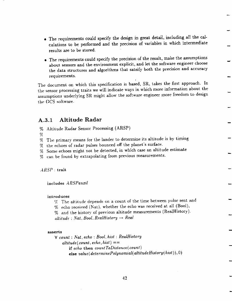
• The requirements could specify the design in great detail, including all the cal-

culations to be performed and the precision of variables in which intermediate

results are to be stored.

• The requirements could specify the precision of the result, make the assumptions

about sensors and the environment explicit, and let the software engineer choose

the data structures and algorithms that satsify both the precision and accuracy

requirements.

The document on which this specification is based, SR, takes the first approach. In

the sensor processing traits we will indicate ways in which more information about the

assumptions underlying SR might allow the software engineer more freedom to design

the GCS software.

A.3.1

%

%%

Altitude Radar

Altitude Radar Sensor Processing (ARSP)

The primary means for the lander to determine its altitude is by timing

the echoes of radar pulses bounced off the planet's surface.

Some echoes might not be detected, in which case an altitude estimate

can be found by extrapolating from previous measurements.

ARSP " trait

includes A RSPauzil

introduces

cX The altitude depends on a count of the time between pulse sent and

% echo received (Nat), whether the echo was received at all (Bool),

% and the history of previous altitude measurements (RealHistory).

altitude • Nat, Bool, RealHistory --_ Real

asserts

V count : Nat, echo : Bool, hist : RealHistory

altitude (count, echo, hist ) --if echo then countToDistance( count )

else value ( determinePolynomial( altitudeHistory ( hist ) ), O)

42

%%%%%%%%%%%%

%%%%

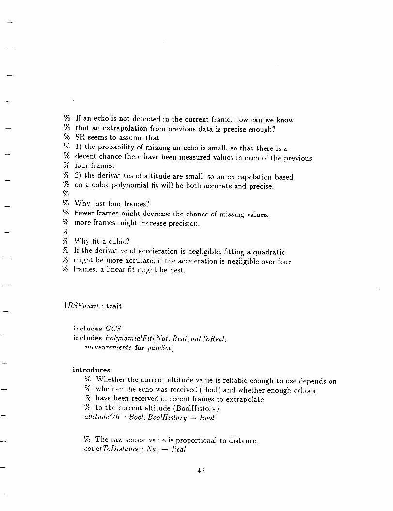
If an echo is not detected in the current frame, how can we know

that an extrapolation from previous data is precise enough?SR seems to assume that

1) the probability of missing an echo is small, so that there is a

decent chance there have been measured values in each of the previousfour frames;

2) the derivatives of altitude are small, so an extrapolation based

on a cubic polynomial fit will be both accurate and precise.

Why just four frames?

Fewer frames might decrease the chance of missing values;

more frames might increase precision.

Why fit a cubic?

If the derivative of acceleration is negligible, fitting a quadratic

might be more accurate: if the acceleration is negligible over four

frames, a linear fit might be best.

ARSPauzil • trait

includes GCS

includes PolyT_omialFit( Nat, Real, nat ToReaI,

measurements for pairSet )

introduces

% Whether the current altitude value is reliable enough to use depends on

% whether the echo was received (Bool) and whether enough echoes

% have been received in recent frames to extrapolate

% to the current altitude (BoolHistory).

altitudeOK : Bool, BoolHistor9 _ Bool

% The raw sensor value is proportional to distance.

count ToDistance • Nat _ Real

43

A R_frequency, speedOfLight .4 Real

% Extrapolation is based on a set of recent altitude measurements.

altitudeHistory : RealHistory ---* measurements

asserts

V echo : Bool, hist : BoolHistory

altitudeOK ( echo, hist ) = =

echoV

(hist[O] A hist[1] A hist[2] A hist[3])

V count : Nat

count ToDistance (count) ==

(nat ToReal( count ) * speedOfLight)/AR-frequency

V hist • RealHistory

altitudeHistory( hist ) ==

{[1, hist[O]], [2, hist[1]], [3, hist[2]], [4. hist[3]]}

44

A.3.2 Accelerometers

Accelerometer Sensor Processing (ASP)%%% The lander has three accelerometers, one for each coordinate axis.

% ASP converts the readings from these sensors into an acceleration vector

% by scaling, adjusting for temperature, and correcting for misalignment.

% The readings have a small but significant probability of being very

% inaccurate, so ASP filters the data by comparing each measurement with

% previous ones and replacing any flaky value with an average.

ASP : trait

includes ASPauxil

introduces

Acceleration depends on the raw sensor values (NatTriple),

% the temperature (Real), the acceleration history (RealVectorHistory),

c_ and the history of whether an acceleration component is based on

% a measurement or is an average (BoolTripleHistory).

acceleration : Nat Triple, Real,

ReaIVectorHistory, BootTripleHistory _ ReaIVector

asserts

V count : Nat Triple. temp : Real, i : coordinate,

ah : ReaIVectorHistory, bh : BooITripleHistory

c_. If recent, measurements are reliable, force the current measurement

% to be the average of recent measurements.

acceleration( count, temp, ah, bh )[i] --

if accelerationOK ( count, temp, ah, bh )[i]

then adjustedAccel( count, temp)[i]

else mean( recent( ah, i ) )

45

%%%%%%%%%%%

%%

How can we guarantee the current acceleration value has the required

precision? By comparing with recent measurements,

by assuming that changes to acceleration are negligible between frames,

and by assuming that the probability of a flaky measurement in any given

frame is small.

SR prescribes replacing a flaky measurement with an average

of the most recent three acceleration values,

but only if each of the three was itself near the mean.

This ad hoc method leads to the funny situation that the current

measurement is considered more reliable if its predecessors are less so.

Why three values?

Why not use several of the most recent uncorrected values?

ASPauxil : trait

includes GCS

includes Statistics

introduces

% Whether the current acceleration components are based on measurement

_, or on an average, depends on the same factors as does the acceleration.

accelerationOK : Nat Triple, Real,

Real l/ectorHistory, BoolTripleHistory _ BooITriple

_7_ Convert raw values to an acceleration vector.

¢7_, The conversion gain, A_gain, depends on temperature.

measuredAccel : Nat Triple. Real _ ReaIVector

A_gain : Real _ ReaIVector

A_gain o. A_bias : _ ReaIVector

91, 9_ :--* Real

% Adjust for misalignment of the accelerometers.

% The adjustment is expressed bv a constant tensor.

adjustedAccel : Nat Triple, Real ---, RealVector

alpha_matrix :---* RealTensor

% Are recent measurements good enough for comparison with current?

recentOK : BoolTripleHistory _ BoolTriple

46

% What is the rangeof believableaccelerationvalues?% The rangeis a constantmultiple of the standard deviation% of recent accelerationvalues.minAccel,mazAccel: RealVectorHistory _ RealVectorA_scale :---* Real

% Put the recent acceleration values into a bag.

recent : Reall/_etorHistory, coordinate _ RealBag

asserts

V count : NatTriple, temp : Real, i : coordinate,

ah : RealVectorHistory, bh : BoolTripleHistory

% The current acceleration value is considered reliable

% if it couldn't be, or didn't need to be, forced near the average.

accelerationOK ( count, temp, ah, bh )[i] --

(--,( recentOI(( bh )[i] ) )V

between( minAccel( ah )[i],

adjustedAccel( count, ternp )[i],

maxAccel( ah )[i])

V count : NatTriple, temp : Real, i: coordinate

A_gain(temp)[i] --

A-gaino[i]+

((ga * letup)+

(gz * (temp_2)))

m easu redA ccel( count, temp)[i] --

A_bias[i] + ( a_gain( temp)[i] • natToReal( count[i]) )

V count : Nat Triple, temp : Real

adjustedAccel( count, temp ) --

alpha_matrix ® measuredAccel( count, temp )

V h : BoolTripleHistory, i : coordinate

recentO1_" (h )[i] --

(h[0])[i]/X (h[1])[i] A (h[2])[i]

V h : RealVectorHistory, i : coordinate

47

recent(h, i) =={(h[0])[i], (h[1])[il, (h[2l)[i] }

minaccel(h)[i] -=mean(recent(h, i))-(A_scale * standardDeviation( recent( h, i) ) )

ma_Accel(h)[i] ==mean(recent(h, i) )+

(A_scale • standardOeviation( recent(h, i)))

A.3.3

%CA

%%

Gyroscopes

Gyroscope Sensor Processing (GSP)

The lander has three gyroscope sensors, each permitting a measurement

of the rate of rotation around an axis.

There is one gyroscope sensor for each of the lander's coordinate axes.

GSP converts the raw sensor data into a angular velocity psuedo-vector

by scaling, and by adjusting for temperature.

For brevity, we're also calling the angular velocity "spin".

GSP" trait

includes GSPauxil

introduces

The spin vector depends on three measurements of rotation speed

cA (NatTriple), three measurements of rotation direction (senseTriple),

% and temperature (Real).

spin • Nat Triple, sense Triple, Real _ RealVector

asserts

V count : Nat Triple, dir:senseTriple, temp: Real, i: coordinate

spin( count, dir, temp )[i] --

if dir[i] = counterClockWise

then rate( count, temp)[i]

48

% SR is unclear whether the sign is part of the rate calculation or not.

GSPauzil : trait

includes GCS

introduces

% The rotation rate around each axis is independent of direction,

% depending only on speed and temperature (unclear from SR).

rate : NalTriple, Real ---* RealVector

G_offset :---_ RealVector

% The gain for converting from counter values to speed depends on

% temperature.

G_gain : Real _ RealVector

G_gain o :--_ RealVector

93,94 :---_ Real

asserts

V temp : Real, i : coordinate

G_gain(temp)[i] --

G_gaino[i]+((93 * ternp )+

(g4 * (temp'2)))

V count : NatTriple, temp: Real, i : coordinate

,'ate(count,t mp)[i] --G_offset[i]+

( G_gain(temp)[i] • natToReal( co,,nt[i]) )

49

A.3.4

%%%%%%%%

%

%%%%%

%%

Touch Down Landing Radar

Touch Down Landing Radar Sensor Processing (TDLRSP).

The lander has four Doppler radars, each of which measures the vehicle's

speed in a single direction: along one radar beam.

Each speed is the projection of the vehicle's velocity vector along

the beam direction.

TDLRSP combines the speed measurements into an estimate of the velocity.

The raw sensor data for each radar consists of a counter value and a

boolean indicating whether the count is meaningful in this processing frame.

So there may be anywhere from 0 to 4 speed measurements available in a frame.

The velocity vector has three components, which will be determined

by three measurements of speed in independent directions.

Therefore the velocity may be either overdetermined or underdetermined,

depending on the number of speed measurements.

TDLRSP takes an average if four speeds were measured.

If fewer than three speeds were measured. TDLRSP reports which velocity

components have been determined (some may be determined even if not all are

because the radars are symmetrically placed in the vehicle coordinate

system, in which the velocity is to be calculated).

TDLRSP" trait

includes TDLRSPauzil

includes Matrix( RealMatrix. coordinate, Real, RealVector for array)

includes L _nearEquatwn( Real Vector. RealMatriz, coordinate. Real,

BoolTriple for BoolArray)

introduces

% The raw sensor data will be a NatQuad and a BoolQuad.

% From this data the following two operators extract

% 1) the velocity vector and

% 2) a boolean for each vector component in the vehicle coordinates,

% telling whether the component has been uniquely determined.

velocity: NatQuad, BoolQuad _ RealVector

velocityOh" : NatQuad, BoolQuad _ BooITriple

% An average of four determinations of velocity is defined as

50

% a component-wiseweighted average.% Each weight is 1 if its correspondingvelocity component is determined,% 0 if it is underdetermined.% Two auxiliary operators aredefined:% a weighted product, and the sumof the weights.average: RealVectorQuad, RealVectorQuad _ ReaIVector

17 : RealVectorQuad, RealVectorQuad ---. RealVector

S : RealVectorQuad --_ ReaIVector

% Four constraints, one for each beam, can be used to determine

% three velocity components in four ways by ignoring each% beam in turn.

% vel is the quad of solutions gotten in this way.

% OK is a matrix of weights: 1 if a vector component is determined,_, 0 otherwise.

vel : NatQuad --, RealVectorQuad

Oh': NatQuad, BoolQuad --, RealVectorQuad

c7(_ Ignoring one of the four beams yields triples of vectors.

Yc To express linear equations having these triples as coefficients,

e/c we must convert vector triples to matrices.

vector Tripte ToMatrix : RealVector Triple _ RealMatrix

asserts

V nq : NatQuad. bq : BoolQuad, i: coordinate

velocity( nq, bq ) == average( vel( nq ), OIi ( nq, bq) )

velocityOh(nq, bq)[i]---= _(OK(nq, bq))[i] > 0

V nq : NatQuad. b: beam

vel(nq)[b] --

solve( ignore(b, beam Velocity( nq ) ),

vector Triple ToMatrix ( ignore(b, TDLR_angles ) ) )

V nq : NatQuad, bq : BoolQuad, b : beam, i : coordinate

( Oh'(nq, bq)[b])[i] --

if determine( ignore(b, bq),

ignore(b, beam Velocity(nq)),

vector Triple ToMatrix( ignore(b, TDLR_angles )))[i]then 1

else 0

51

V value, weight : ReaIVectorQuad, i : coordinate

average(value, weight )[i] ==

17(value, weight )[i]/ S,( weight )[i]

17(value, wei9ht ) ==

((valuer1] * weight[I])+

(value[2], weight[2])+

(value[3] * weight[3])+

(value[4] * weight[4]))

S(weight) ==

weight[l] + weight[2] + weight[3] + weight[4]

'¢ t : RealVectorTriple, i : coordinate

row( vector Triple ToMatriz( t ), i) == t[i]

TDLRSPauziI : trait

includes GCS

_ Because there are four radars, many quantities appear in fours.

% These "'quad" sorts are axiomatized using the "Quad" trait.

includes Quad( RealQuad, RealVector, Real)

includes Array( RealVector Triple, coordinate, RealVector )

includes Quad ( Real VectorQuad. Real Vector Triple. Real Vector)

includes Quad( NatQuad. Nat Tripte. Nat)

includes Quad( BoolQuad, BooITriple, Bool)

i nt rod uces

% Each beam's count is converted linearly to a speed,

% using constant gain and offset.

beam Velocity : NatQuad _ ReaIQuad

TDLR_gain, TDLR_offset :---, Real

% Four vectors of direction cosines in the vehicle coordinates

% determine the beam directions.

TDLR_angles :4 RealVectorQuad

52

cos_alpha, cos_beta, cos_gamma :---* Real

asserts

equations

TDLR_angles[1] == [cos_alpha, cos_beta, cos_gamma]

TDLR_angles[2] == [cos_alpha,-cos_beta, cos_gamma]

TDLR_angles[3] == [cos_alpha,-cos_beta,-cos_gamma]

TDLR_angles[4] == [cos_alpha, cos_beta,-cos_gamma]

V nq: NatQuad, b:beam

beamVclocity(nq)[b]--TDLR_offse! + ( TDLR_gain * natToReal( nq[b]) )

53

A.3.5

%%%%

Temperature

Temperature Sensor Processing (TSP)

GCS needs a measurement of temperature in order to correct its

accelerometer and gyroscope readings.

% The lander has two temperature sensors:

% one solid-state, the other a matched pair of thermocouples.

% The solid-state sensor is accurate over a greater range,

eA while the thermocouples are more precise.

_: TSP yields the most precise temperature measurement.

TSP : trait

% The calibration of TSP involves polynomial fitting.

includes PolynomialFit ( Nat, Real, nat ToReal,

calibration for pairSet )

includes DerivativeFit ( Nat. nat ToReal)

includes GCS

introduces

0_ The temperature depends on reading from both the solid-state (Nat)

and thermocouple (Nat) sensors.

temperature : Nat, Nat _ Real

tempSS : Nat _ Real

temp Thermo : Nat _ Real

inRange Thermo : Nat _ Bool

% most precise temperature

% solid-state sensor temp

% thermocouple pair sensor temp

% accurate range of thermocouples

_ The solid-state sensor is linear.

% Its calibration consists of two measurements.

ml,m2 :_ Nat

tl, t2 :---_ Real

calibrateSS :4 calibration

% The thermocouple pair is linear between its calibration points.

m3. m4 :---* Nat

t3, t4 :---, Real

calibrate Thermo :---, calibration

% The thermocouple pair is accurate for readings + or - 15 percent beyond

54

%%

% the second, first, and zeroth derivatives.

min, max :4 Real

slope :--* Real

extrapolate :---, Real

upperCalibration, lowerCalibration :---* RealSequence

its calibration points. Beyond the calibration points, its response

is quadratic. The calibration in the quadratic regions consists of

% 15 percent

asserts

equations

calibrateSS== {Ira1, Imp,calibrate Thermo == {[m3, t3], [m,, Q]}

rn 3 < rn 4

min == natToReal(m3) - (extrapolate • (natToReal(m, @ m3)))

max == natToReal(m,) + (extrapolate • (natToReal(m, @ m3) ))slope == (t, - t3)/natToReal(m, @ m3)

upperCalibration == [2, slope, t4]

lowerCalibration == [-2, slope, t3]

V nSS, nTh: Nat

temperature ( nSS , n Th ) --

if inRange Thermo( n Th )

then temp Thermo( n Th )

else tempSS( nSS)

V 7_ : Nat

inRange Thermo( n ) = = between ( rain. nat ToReal(n ), max )

tempSS(7_) --

value( determine Polynomial (calibrateSS ) , n)

t emp Thermo( 7_) --

if n > m4

then

value ( determinePolynomial(m4, upperCalibration ), n)

else if n < rn3

then

value( determinePolynomial (m3, lowerCalibration ), n)

else

value (determinePolynomial ( calibrate Th ermo ), n)

55

A.3.6 Guidance

%%%%%%%

Guidance Processing (GP)

Computations in GP are needed

to find acceptably precise values for velocity and altitude if

the measured values in the current frame are unreliable.

The measured value of velocity comes from TDLR.

The measured value of altitude comes from AR.

GP : trait

includes GCS

includes Rotation(attitude for integrate )

includes TDLRSP

includes ARSP

introduces

% CCS's best estimate of the current velocity depends on TDLR

% (NatQuad and BoolQuad) if that measurement exists, or on

% an integration using velocity, acceleration, and spin

% (RealVectorHistory**3) if it doesn't exist.

velocity: NatQuad. BoolQuad,

Real VectorHistory, Real VectorHistory, Real VectorHistory ---* ReaIVector

"File integration is simply a modification to the previous velocity (Real)

using the current acceleration (RealVector) and

% the history of angular velocity (RealVectorHistory).

velocitylntegral : Real Vector, ReaIVector, RealVectorHistory --* ReaIVector

% GCS's best estimate of the current altitude depends on ARSP

% (the first four args) if that measurement is reliable, or on

% integration using velocity and spin (the last two args)

% if the measurement isn't reliable.

altitude : Nat, Bool, RealHistory, BoolHistory,

RealVectorHistory, RealVectorHistory _ Real

The integration is a modification to the previous altitude (Real)

56

% using the current velocity (RealVector) and the history of

% angular velocity (RealVectorHistory).

altitudelntegral : Real, RealVector, RealVectorHistory _ Real

% Which way is down depends on the history of rotations.

down : RealVectorHistory---. RealVector

% The acceleration due to gravity

gravity : _ Real

asserts

V nq : NatQuad, bq : BoolQuad,

vel, accel, spin : RealVectorHistory, i : coordinate

velocity( nq, bq, vel, accel, spin )[i] --

if velocityOl( (nq, bq)[i]

then velocity( nq, bq)[i]

else velocitylntegral( now( vel). now( accel), spin )[i]

% from TDLR

cA A new value for velocity is gotten by

% 1) using the current spin to change coordinates of previous velocity;

% 2) adding the measured acceleration in the lander's inertial

% reference frame (measured in the new vehicle coordinates);

% 3) adding the acceleration due to gravity of the inertial frame.

V vel, accel: RealVector, spin : RealVectorHistory

velocitylntegral( vel, accel, spin ) --

( vector To Tensor( delta_t • now(spin)) @ vel)+

(delta_t • accel)+

( delta_t * (gravity • down(spin)))

V count : Nat, echo : Bool, all : RealHistory, bh : BoolHistory,

vel. spin : Reall'_ctorHistory

altitude(count, echo, alt, bh, vel, spin) --

if altitudeOh" ( echo, bh )

then altitude(count, echo, alt )

else altitudelntegral( now( alt ), now(vel), spin)

% from AR

% A new value for altitude is gotten by subtracting

% the downward projection of velocity from the old value.

V all : Real, vel : RealVector, spin : RealVectorHistory

altitudelntegral ( all, vel, spin ) --

57

art - (do,,,,,(spin). vel)

% "down" is a vector pointing toward the planet.

% We need it expressed in the lander's coordinates.

% Assuming the spin history records rotation starting with the lander

% vertical, then down is the coordinate transformation of the x axis.

V spin : RealVectorHistory

down(spin) ==

attitude(spin) ® unit(x)

A.4 Actuator Control

58

A.4.1

%%%

Axial Engines

%%%%

%%%%%%

cZ

%

%

%%

Axial Engine Control Law Processing (AECLP)

The lander has three main engines parallel to its vertical axis.

These engines provide separately controllable thrust to change the

lander's pitch, yaw, and speed of descent.

AECLP controls the warm-up of the axial engines and, once the engines

are warm, controls the valve settings that determine engine thrust.

This control is based on the current data about the lander's dynamics.

which are in turn computed from sensor data.

AECLP is intended to keep the lander's vertical axis aligned with the

lander's velocity vector.

If that is achieved, the axial engines work to slow the lander's descent.

AECLP is intended to keep the lander's speed close to a pre-computed

value that depends on the altitude.

This pre-computed dependence is called the "velocity-altitude contour".

To slow the lander down, more thrust is needed uniformly from all engines.

To alter pitch or yaw, torque is supplied by differences in the

thrust from the three axial engines.

Some key sorts used in AECLP are defined in AECLPauxil.

Some AECLP definitions differ from SR's because SR seems to have

negated certain quantities for unknown reasons.

.4 ECL P : trait

includes AECLPauxil

int rod uces

% AEcommand defines a NatTriad of correct valve settings

% based on available data about altitude (RealHistory), velocity,

% acceleration, angular velocity (RealVectorHistory**3),

% the current integrated thrust (Real), and the current phase of descent.AEcornmand :

RealHistory,

Real VectorHistory ,

59

Real Vector History ,

ReaI Vector History ,

Real,

phase --* Nat Triad

% The valve settings are a linear function of the correcting force

% needed to control pitch, yaw, and thrust.

thrust : Real, Real, Real _ Nat Triad

gPl, gP2, gPY :'* Realcoefficients

Constants used in defining thrust

TE_init :---, Real

TE_drop :---* Real%

% thrust while warming engines

thrust while dropping to contour

% Conversion from real values to valve settings.

convert : Real ---, Nat

factor :----_Real% 127

% The "integrated thrust" referred to previously is part of

% the control state updated in trait Frame.

% When the integrated thrust is used in AEcommand to compute the new

% thrust, however, its value is limited by this function:

e ThrustL : Real ---* Real

TE_min, TE_max :_ Real

% Similarly, the restoring torques for pitch and yaw are limited

c7_ bv these functions:

ePitchL, e }'awL : Real ---, Real

PE_min, PE_max :_ Real

YE_min, YE_maz :4 Real

% Apparently to avoid sudden changes in thrust,

% the computed thrust is integrated.

% Euler integration is explicitly specified;

% to do this we add a component to the GCS state,

% saving the value of the thrust integral in the spec.

e_, Tile first argument to eThrust is the result of PID control.

% The second argument is the previous thrust integral.

e Thrust : Real, Real ---* Real

omega , g a :---_ Real% coefficients

6O

asserts

% AEcommand is determined differently for different phases of the descent.

%

_/ alt : RealHistory, vel, ace, spin : RealVectorHistory, thr : Real, ph : phase

AEcommand( all, vel, ace, spin, thr, ph ) --

if ph.engine = cold V ph.landing

then 0

else if ph.engine = warming

then thrust(

gq• now(spin)[y],gr * now(spin)[:],TE_init )

else if ph.contour

then thrust(

ePitchi( ePitch( currentPitch( spin, vel) ) ),

eYawL(eYaw(currentYaw(spin, vet))),e ThrustL( e Thrust (

e i_l( currentSpeed(alt, vel, acc)), thr)))

else thrust(

ePitch L( ePitch ( current Pitch (spin , vel ) ) ),

e YawL( e Yaw ( current Yaw (spin, vel) ) ),

TE_drop)

% all engines off

% differs from SR

V ePitch, eI'aw, eThrust : Real

thrust( ePitch, e Yaw, e Thrust)[1] --

convert((gpl * ePitch) + eThrust)

thrust( ePitch, e }'au,, e Thrust)[2] --

convert(((gp2 * ePitch) - (gpy * eYaw)) + eThrust)

thrust( ePitch, e Yaw, e Thrust)[3] --

convert(((gp: * ePitch) + (gpy * eYaw)) + eThrust)

V ,': Real

convert(r) == reaIToNat(factor • cutoff(O, r, 1))

V r : Real

e ThrustL( r ) == cutoff( TE_min, r, TE_max )

ePitchL(r) == cutoff (PE_min, r, PE_max )

e YawL(r) == cutoff( YE_min, r, YE_max)

61

% Integrate the direct calculation for thrust.

% Omega is the time constant for the integration.

V control, thr:Real

e Thrust ( control, thr) ==

((ga * control * delta_t) + ((1 - (omega * delta_t)) * thr))

AECLPauzil : trait

includes GCS

includes Integration (RealHistory, Real, delta_t )

% The thrust is controlled according to a proportional-integral-derivative

% (PID) control law. This means the control is a linear function of position

% in a three dimensional "configuration space" formed by

_ an axis for the error, or deviation from the desired value (P),

_ an axis for integral of the error (I), and

_, an axis for tile derivative, or rate of change, of the error (D).

%

configuration tuple of

error: Real,

integral:Real.rate: Real

v

% Because there are three engines, many quantities appear in threes.

(Z We include traits for arrays of Real and Nat.

engine enumeration of 1,2.3

includes Array{ RealTr_ad. engine. Real)

includes Array( NatTriad, engine, Nat )

i nt rod u ces

% The PID control laws each map a configuration into a real number

% proportional to the correcting force.

ePitch, e Yaw, e Vel : configuration _ Real

N, Constants used in PID control

gq, gw, gwi :--, Real

gr, gv, gvi :---* Real

gaz, gve, gvei :---* Real

% pitch

% yaw

% thrust

62

The current configurations for pitch, yaw, and speed

% are extracted from histories, integrating where necessary.

currentPitch, current Yaw :

Real VectorHistory ,

Real VectorHistory ---, configuration

currentSpeed :

ReaIHistory,

Real Vector History ,

RealVectorHistory ---* configuration

% To express the integrals of pitch and yaw,

% we first form the histories of these quantities.

pitchHistory, yawHistory :

RealVectorHistory _ ReaIHistory

_, The speed error is the deviation from a pre-computed¢7_ "'velocity-altitude contour".

GCS tries to follow this contour.

% speedError depends on the histories of altitude and velocity.

speedError :

RealHistory,

RealVectorHistory ---, RealHistory

(_ The precomputed speed that the lander should have at a given altitude.

velocityAltitudeContour :Real _ Real

asserts

V pttch: configuraltol_

ePitch(pitch) --

(gq * pitch.rate)+

(g w • pitch.error)+

(gwi * pitch, integral)

V yaw : configuration

e Yaw ( yaw ) ---

(9r * yaw.rate)+

(gv * yaw.error)+

(gvi * yaw.integral)

% differs from SR

63

V velError: configuration

e Vel(velError) ==

(( - gaz ) * velError, rat e) +

(gve • velError.error)+

(gvei • velError.integral)

% The history of pitch and yaw angles is gotten from the

% 3-dimensional history of velocity

% expressed in the lander's coordinates.

% Because we only care about differences between the velocity vector

% and the lander's x-axis (vertical),

% pitch is the angle between them in the x-z plane, and

% yaw is the angle between them in the x-y plane.

% The small-angle approximation is used in this specification,

% which is an optimistic assumption about the control.

V velH : Real l/ectorHistory, i : Nat

pitchHistory( velH )[i] == ( veIH[il)[zl/( veIH[i])[x]

yawHistory( velH )[i] == -( ( velH[i])[y]/ ( veIH[i])[z])

_, definition of vaw differs from SR

% The angular velocity measurement provides the derivatives of

% pitch and yaw.

_/ spin, vel : RealVectorHistory

currentPitch ( spin, vel ) --

[now( pitchHistory( vel ) ),

integrate(pitchHistory( vel) ),

,,ow(spi,, )M]current Yaw(spin, vel) ---

[now( yawHistory( vel ) ).

integrate( yawHislory( vel ) ),

now(spin)[z]]

% The speed error is the difference from the precomputed speed

% the lander should have.

V altH : RealHistory, velH : RealVectorHistory, i: Nat

speedError( altH, velH )[i] --

leagth ( velH [i]) - velocityAltitude Contour ( altH [i])

% The acceleration measurement provides the derivative of

°A speedError. This is an approximation that assumes:

% 1) changes in the velocity-altitude contour are small compared to

64

% the acceleration;% 2) the componentsof velocity and acceleration along the lander's

% vertical axis are much larger than the other components.

V all : RealHistory, vel, acc: ReaIVectorHistor v

currentSpeed( alt, vet, acc ) --

[now( spe_dEr,'o,'( alt, ,,el) ),integrat e( speedError( alt, vel) ),

nowlacc)[z]]

A.4.2

%%%%V

%

%_Z

Roll Engines

Roll Engine Control Law Processing (RECLP)

The lander has three opposing pairs of roll engines mounted on its sides

perpendicular to the vertical axis.

Firing these engines provides torque around that axis. and can be usedto control roll.

REC, LP attempts to maintain the roll angle at a fixed reference pointdetermined at initialization.

(This reference point seems to have no physical significance, because

the lander is simultaneously rotating around the other axes too.

However. if the rotation is not too violent, fixing the roll angle

may be sufficient stability for controlling the axial engines.)

RECLP : trait

includes RECL Pauxil

includes lntegratwn( RealHistory, Real, delta_t )

introduces

% The roll engines will be fired with an intensity and direction

% determined by the history of vehicle rotation (RealVectorHistory),

% and the current phase of the descent.

% (Do not confuse the phase of descent with phase space.)

REinten_ity : Real l.ectorHistorg, phase _ REintensity

REsense : RealVectorHistory _ sense

65

% The roll rate is simply the x componentof the spin vector.% The roll angle is gotten by integrating the rate.% The combination of angleand rate forms a phasespacefor roll.currentPhasePosition : RealVectorHistory "* rollPhaseSpace

% The roll rate is one of the components of spin, and

_. so can be projected out.

rollHistory : ReaIVectorHistory _ ReatHistory

asserts

V spin : RealVectorHistory, ph : phase

REint ensity (spin, ph ) --

if ph. engine = cold V ph.landing

then off

else REpulse( currentPhasePosition( spin ) )

REsense (spin) ==

REdirection(currentPhasePosition(spin))

V spin: RealVectorHistory, n:Nat

currentPhasePosition( spin ) ==

[integrate( ,'ollHistory( spin ) ),

no, (spin)[z]]

rollHisto,'y( spin )In] == (spin[n])[x]

66

RECLPauziI" trait

includes GCS

REintensity enumeration of off, minimum, intermediate, maximum

rollPhaseSpace tuple of

angle : Real,

rate • Real

introduces

t){ The intensity and direction depend only on position in the

% roll phase space. The phase space is divided into rectangular

% regions using some constants as boundaries.

% (This seems unnecessarily ad hoc to me; why not use a PD control law

% similar to those for pitch and yaw in AECLP? The thrust

_ determined by this control law would need to be quantized in that case,

of course, but the same is true for AECLP.)

REpuls_ : rollPhascSpac_ ---, REintensity

REdirection : rollPhaseSpace ---, sense

thetal, theta2 :----, Real

Pl , P2, Pa, P4 :-'_ Real

asserts

V roll • rollPhaseSpace

REdirection( roll ) --

if ( roll. rate 2 P4 )V

(roll.rate >_ t)1 A between(O, roll.angh, r,))V

(roll.rate >_ 0 A between( thetal, roll.angle, rr) )V

( roll.rat¢ >_ (-P3)A between(theta2, roll.angle, r:))then clock Wise

else counterClock Wise

REpulse(roll) --

if roll.rate < 0

then

REpulse([- ,.oll.a,gl . -roU.,atd)else

if ( between (p3, roll. rate, P4 )A

bet ween ( - r:, roll.angle, 0))V

67

(be tween (0, roll. rat e, p4 )/_

between (- theta 2, roll. angle, 0))V

(between (0, roll. rate, pl ) A

between (0, roll. angle, thetal ))

then off

else

if between (0, roll.rate, Pl )A

between ( thetal, roll. angle, theta2 )

then minimum

else

if between(pl . roll.rate, p_ )A

between (0, roll. angle, theta 2)

then intermediate

else mazimum

68

A.5 I/O Interface

% This trait defines the connection between the sorts used throughout

% the rest of the specification and the sorts that model details of

% input and output registers used by GCS.

Interface : trait

includes Frame

includes Communication

8- 16- and 32-bit registers are used in GCS I/O.%

includes Register(8, 8bit for register)

includes

includes

includes

includes

Register(16, 16bit for register)

Map( 16bit Triple. coordinate, 16bit )

Map( I 6bit Triad, engine, 16bit )

Map( 16bitQuad, beam, 16bit)

includes Register(32, 3_bit for register)

includes Map( 32bitQuad, beam, 3Obit )

% Define the concrete representation of the sensor data sort

% used in trait Frame. All registers are 16 bit except the counters

used to keep TDLR unlocked for an interval of time.

iTzpul tuple of

AR_counter : 16bit.

A_counter: 16bitTriple,

G_counter : 16bit Triple,

TDLR_counter : 16bitQuad,

SS_temp : 16bit,

Thermo_temp : 16bit,

TD_counter : 16bit.

TDLR_unlocked : 32bitQuad

tT_ Define the concrete representation of the actuator data sort

69

% usedin trait Frame.%

output tuple of

AE_cmd : 16bitTriad,

RE_cmd : 16bit,

chute_released : Bool

% Define the concrete representation of communication packets

% used in trait Communication.

%

commOutpul tuple of

pattern: 16bit,

number : 8bit,

variables : bitSequence,

checksum: 16bit

introduces

_?_ Abstraction functions map the concrete sorts into the abstract.

abstract • input _ sensor

abstract • output _ actuator

abstract • commOutput ---* packet

t/,

c/,,

update :input ---, il_putTDLR_lock_time :---* Real

There is only one instance of concrete I/0 state being preserved

from one frame to the next. This instance is in TDLRSP, where

counters record how long until each radar beam can be locked again.

The update function tells how this concrete I/O state is modified

between frames.

a constant

o_ Roll engine intensities are coded ill 2 bits.

This function decodes those bits.

REconvert • Nat _ REintensity

% The GCS programmer must choose a set of variables to be communicated

¢7_. and a packing of these variables into a sequence of bits.

c_ This function unpacks those bits.

% We do not specify any properties of the packing.

unpack : bitSequence ----,setOfVariables

7O

asserts

% Ifthe altimeter input isnot allones,

% take the value in the lowest 10 bits.

V in : input

abstract( in ).AR_counter_Off --

-,allOnes ( in.AR_counter )

"-,allOnes ( in. A R_counter )

abstract( in ).AR_counter = value( in.AR_counter, [0, 10])

_c Use all 16 bits to get an accelerometer value.

V i7_ : input, i: coordinate

abstract( in ).A_counter[i] == value( in.A_counter[i])

% Bit 15 is the sign; use lowest 14 bits for gyroscope value.

V in : input, i : coordinate

abstract(in), a_counter[i] --

value (in. G_counter[ i], [0, 14])

abstract( in ). G_counter_sense [i] --

if ( in.G_counter[i])[15]then clock Wise

else counterClock Wise

The TDLR value is tile full 16 bits in the register when

(/( the value is not zero and the _unlocked counter has reached zero.

V il_:input.b: beam

abstract( i7_). TDLR_counter_Oh" [b] --

(aUZeros( TDCR_unlocked[b]))Avalue(in.TDCR_counter[bl)# 0

abstract(in ). TDLR_counter_OK [b]

abstract(in). TOLn_counter[b I = value(in. TDLn_counter[b])

% Use all 16 bits for each temperature sensor.

V in : input

abstract( in ).SS_temp == value(in.SS_temp)

abstract( in ). Thermo_temp == value( in. Thermo_temp )

71

% The touch-down input should be either all ones or all zeros.

V in : input

allOnes( in. TD_counter ) =_ abstract( in ).touch_down

allZeros ( in. TD_counter ) _ -, abstract (in). touch_down

% Each TDLR radar may become "unlocked", after which its

% value is not reliable for a time.

% The TDLR_unlocked counter prevents GCS from using the value

% returned bv a TDLR beam until that time has passed.

% Decrement the TDLR_unlocked counter between frames unless

% it is already zero and the beam is returning non-zero values.

% If the counter has been zero but the beam returns zero,

% reset the counter to the required wait.

V in : input,b: beam

value(in. TDLR_unlocked[b]) > 0

value( update(in). TDLR_unlocked[b]) =

value(in. TDLR_unlocked[b]) t3 1

( value( in. TDLn_unlocked[b]) = OA

value( in. TDLn_counter[b]) = O)

value ( update (in). TDLR_unlocked [b]) =

real ToNal ( TDL R_lock_time / delta _t )

(value( in. TDLR_unlocked[b]) = Oh

value( in. TDLR_counter[b]) > O)

allZeros( update( in ). TDLR_unlocked[b])

(_ All 16 bits matter for each axial engine.

V out : output,e: enginc

abstract( out ).AE_cmd[e] == value( out.AE_cmd[e])

% Show the meaning of the two intensity bits in RE.

V n : Nat

n = 0 _ REconvert(n) = off

n = 1 _ REconvert(n)= minimum

77 = 2 _ REconvert(n) = intermediate

_ = 3 _ REconvert(7_) = maximum

% Bits 1 and 2 hold the intensity: bit 0 the sense.

V out : output

72

abstract (out). RE_cmd_intensity ==

REconvert( value( out.RE_cmd, [1, 2]))

abstract ( out ). RE_cmd_sense --

if out.RE_cmd[O]then clock Wise

else counterClock Wise

V out : output

abstract( out ).release_chute == out.chute_released

% Define the packet corresponding to concrete communication output.

V comm : commOutput

abstract ( comm ).pattern --

value(comm.pattern)

abstract (comm). number --

value( comm. number)

abstract ( comm ).internal --

unpack( comm. variables)

abstract (comm). checksum --

value (comm. checksum)

A.6 Auxiliary Traits

73

A.6.1 Quads

% The Quad trait is used in TDLRSP.

% A quad consists of four objects of the same sort,

% corresponding to the four touch down landing radar beams.

Quad ( quadSort, tripleSort, range) : trait

beam enumeration of 1,2, 3, 4

includes Map( quadSort, beam, range)

coordinate enumeration of x, y, :

assumes Map( tripleSort, coordinate, range)

% The only new operator we define for quads simply throws away one

% of the four components to yield a triple.

% There are four ways to do this, while preserving the original quad order.

cZ

introduces

ignore : beam, quadSort ---, tripleSort

asserts

V q : quadSort

ignore(I, q)[x]

ignore(1, q)[y]

ignore(a,q)[:]

== q[21=: qia]== q[4]

ignore(2,q)[x] == q[1]igno,'e(2,q)[y]== q[31ignore(2,q)[z]== q[41

ignore(3, q)[x] =: q[1]

ignore(3, q)[y] == q[21

ignore(3, q)[z] == q[4]

ignore(4,q)[x]== q[1]ignore(4,q)[y]== q[2]ignore(4,q)[:]== q[3]

74

A.6.2 Rotations

% Rotations are RealTensors that preserve vector length.

% This property of tensors is called

orthogonality.

%%%

7(%%%

%%

%

In three dimensions a unique but ersatz "vector" can be

associated with each rotation tensor.

According to Euler's theorem, each three dimensional rotation has an axis:

the rotation vector lies along this axis and has magnitude proportional to

the rotation angle.

Rotation "'vectors" are ersatz because composition of rotations is not

modeled by vector sum, but by tensor product.

This trait axiomatizes the relation between rotation "vectors" and tensors,

and defines the integral of a history of rotations.

We will need this trait to describe rotations of the lander, so

we define a rotation as a coordinate transformation,

rather than a change in vectors.

rotation :trait

includes Real

includes Vector( RealI,_ctor, Real)

includes Tensor( ReaITensor, Real, RealVector for vector)

includes Hzstory( Real VectorHistory, Real Vector)

introduces

conversions between rotation vector and tensor

vectorTo Tensor : RealVector _ RealTensor

tensorTo Vector : RealTensor _ Real|lector

orthogonal : RealTensor ---* Bool

% Given a sequence of rotation rates specified as vectors,

% where the rates are measured delta apart,

% compose the history of rotations to form a tensor.

integrat_ : Real_ctorHistory _ RealTensor

75

delta :---, Real

% vector length and angle between two vectors.

length : RealVector _ Real

angle : RealVector, RealVector ---* Real

% vectors a,b,c are right handed if c is perpendicular to the plane

% formed by a and b, and a screw turned from a to b advances in

% the direction of c.

rightHanded : RealVector, RealVector, Real Vector _ Bool

asserts

% orthogonal tensors preserve length.

V t : RealTensor, v: RealVector

orthogonal( t ) ::,

length ( t ® v) = length(v)

axiomatize vectorToTensor

V u, v, w : RealVector

orthogonal( vector To Tensor ( v ) )

vector To Tensor( O) == 1

vector To Tensor( v ) @ v == v

( rtghtHanded (w, u, v) A

angle(w, u) = length(v))

( vector To Tensor( v ) @ u) = w % coordinate change

vector To Tensor( r ) --

vectorToTensor(v + (((2 * 7r)/length(v)) * v))

vector To Tensor( v ) @ u = w --

vectorTo Tensor(-v) @ w = u

V t : RealTensor

orthogonal( t ) =*"

vector To Tensor( tensor To Vector (t) ) = t

% Define integration of a sequence of rotations.

V h : RealVectorHistory, e: RealVector

integrate(update(h, e)) ==

76

(delta * vector To Tensor( e ) ) ® integrate(h)

integrate(empty) == 1

% Define length and angle.

V v, w • RealVector

length(v) == root(2, v • v)

v. w == length(v) • length(w)• cosine(angle(v,w))0 < angle(v, w)

angle(v, w) < 7r

% Axiomatize rightHanded.

% A continuity property is also needed to define it completely.

V x, y, z : RealVector

right Handed (z, y, z) =:,

(angle(z, z) = 7r/2A

angle(y, z) = :r/2A

length(x) > OA

length(y) > OA

length(z) > O)

(angle(z, z) = rr/2A

angle(y, z) = 7r/2A

length(z) > 0A

length(g) > 0A

length(z) > O)

( rightHanded(z, y, z) V rightHanded(z, y, -z))

implies

converts vector To Tensor % given linearity of tensors

77

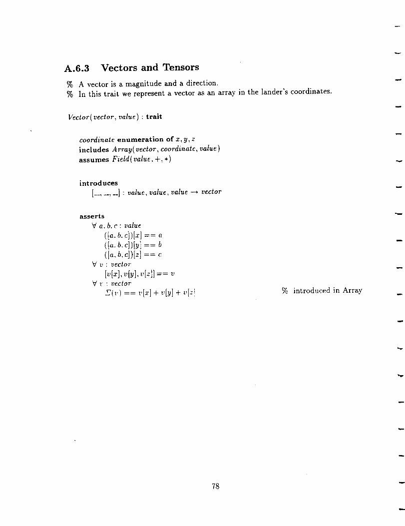
A.6.3 Vectors and Tensors

% A vector is a magnitude and a direction.

% In this trait we represent a vector as an array in the lander's coordinates.

Vector(vector, value) : trait

coordinate enumeration of x, y, z

includes Array(vector, coordinate, value)

assumes Field(value, +, *)

introduces

[..... _]: value, value, value _ vector

asserts

V a. b. c : value

([a. b.c])[x]== a([a.b.c])[y]== b([a,b,c])[z]== c

V v : vector

[v[x], v[y], v[z]] == v

V v: vector

S(_,) == t,[x] + v[y] + v[z] % introduced in Array

78

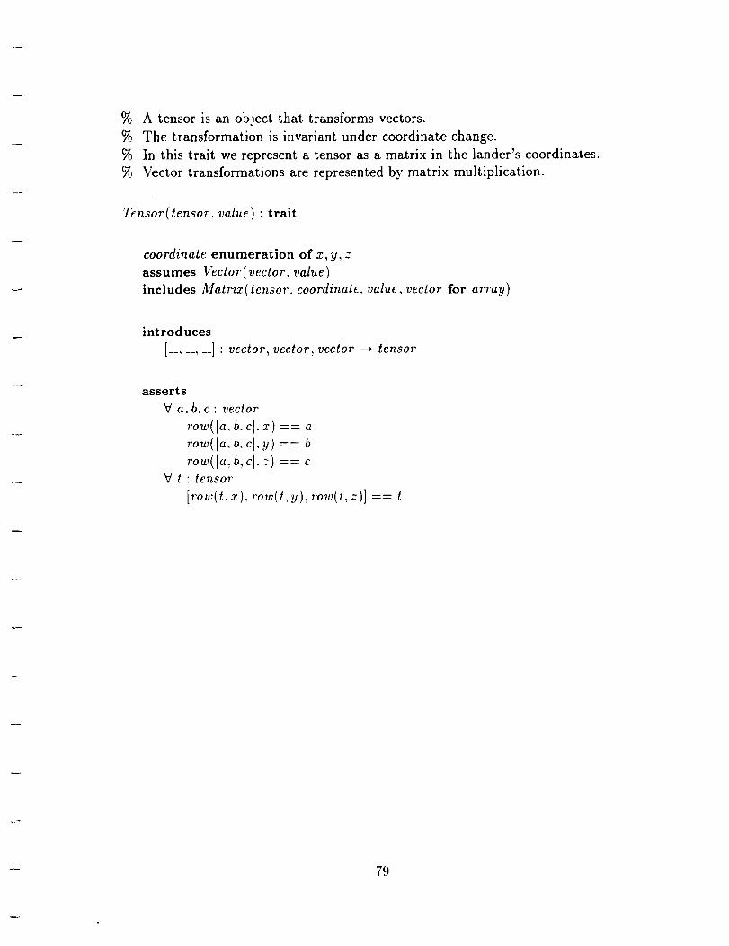
% A tensor is an object that transforms vectors.% The transformation is invariant under coordinate change.% In this trait we representa tensoras a matrix in the lander's coordinates.% Vector transformations are representedby matrix multiplication.

Tensor(tensor, value) : trait

coordinate enumeration of x, y, z

assumes Vector(vector, value)

includes Matrix( tensor, coordinate, value, vector for array)

introduces

[..... , __] : vector, vector, vector _ tensor

asserts

V a. b, c : vector

ro_([a, b.c],_ t ==ro_([_, b.c],y) == brow([,, b,el, :) == c

V t : tensor

[_o_(t, _.),,.o_(t,y), row(t,:)] == t

79

A.6.4 Integration

% Euler integration over histories of events.

% Assume that the events are samples separated in time by delta.

Integration(history, event, delta) : trait

assumes History(history, event )

assumes Field( event, +, *)

introduces

Declare delta to be of the same sort as the events.

delta :--* event

integrate : history --_ event

asserts

(/( The Euler method of approximating an integral is just to sum

¢_ the contributions for each (time) step.

V h :history, e : event

integrate(update(h, e)) == integrate(h) + (delta • e)

integrate(empty) == 0

A. 7 Generic Traits

8O

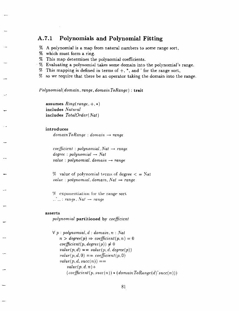
A.7.1 Polynomials and Polynomial Fitting

% A polynomial is a map from natural numbers to some range sort,

% which must form a ring.

% This map determines the polynomial coefficients.

% Evaluating a polynomial takes some domain into the polynomial's range.

_, This mapping is defined in terms of +, *, and " for the range sort,

_, so we require that there be an operator taking the domain into the range.

Polynomial( domain, range, domain ToRange ) : trait

assumes Ring( range. +, .)includes Natural

includes TotalOrder( Nat )

introduces

domain ToRange :domain --_ range

coefficient : polynomial, Nat --_ range

degree : polynomial ---, Nat

value :polynomial. domain ---* range

_: value of polynomial terms of degree < = Nat

value :polynomial. domain, Nat --, range

_ exponentiatioll for the range sort

.... :range. Nat _ i"ang(

asserts

polynomial partitioned by coefficient

V p : polynomial, d : domain, n : Nat

n > degree(p) ::_ coefficient(p,n) = 0

coefficient(p, degree(p)) # 0

value(p, d) == value(p, d, degree(p))

value(p, d, O) == coefficient(p, O)

value(p, d, succ( n ) ) --

value(p, d. n)+

( coefficient (p, succ (n)) • ( domain ToRange (d)"succ(n)))

81

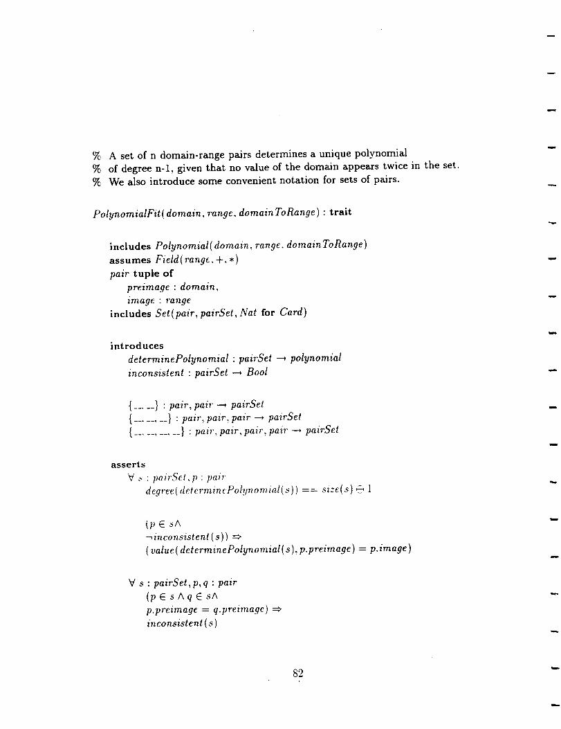
% A set of n domain-rangepairs determinesa unique polynomial% of degreen-l, given that no valueof the domain appearstwice in the set.% We also introduce someconvenientnotation for setsof pairs.

PolynomialFit ( domain, range, domain ToRange ) : trait

includes Polynomial(domain, range, domain ToRange )

assumes Field( range, +, *)

pair tuple of

preimage : domain,

image : range

includes Set(pair, pairSet, Nat for Card)

introduces

determinePolynomial : pairSet _ polynomial

inconsistent : pairSet ---, Bool

{..... } : pair, pair ---, pairSet

{..... , __} : pair, pair, pair --_ pairSet

{ ........... } : pair, pair, pair, pair _ pairSet

asserts

V., : pairSet,p : pair

degree( determincPolynomial(s)) == size(s) __ 1

(p E _A

-,inconsistent (s ) )

( value ( determinePolynomial(s ), p.preimage) = p. image)

V s : pairSet, p, q : pair

(pEsAqEsA

p.preimage = q.preimage)

inconsistent ( s )

82

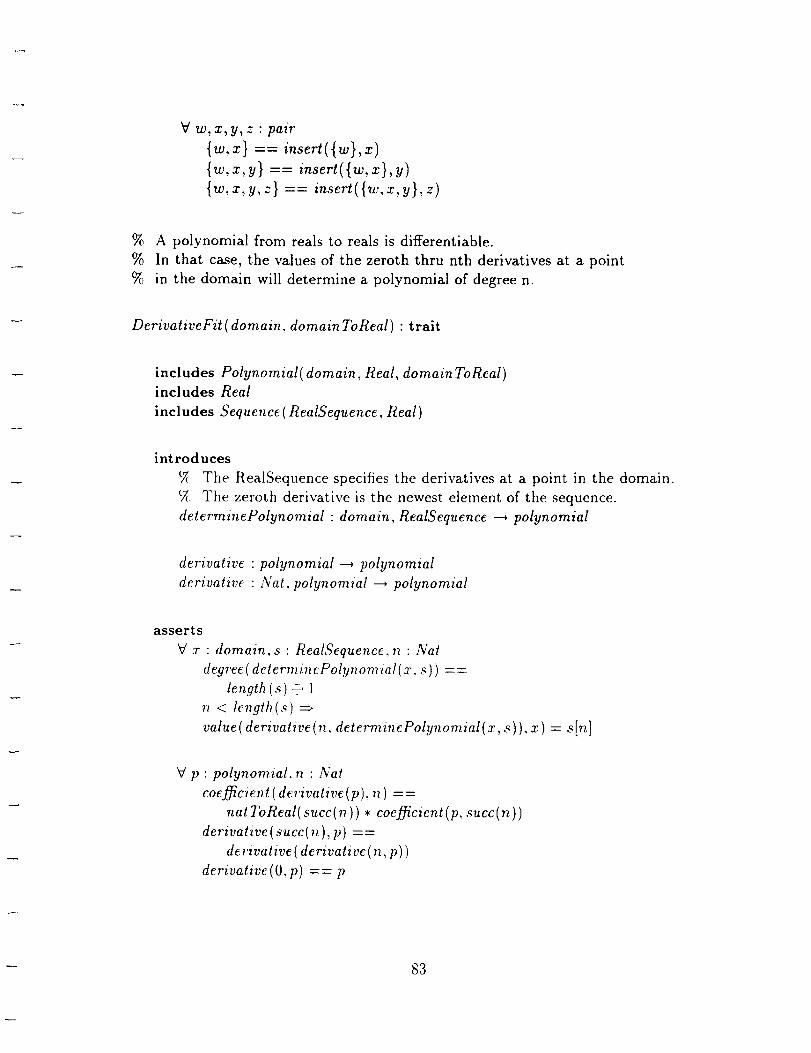
V w,x,y,z : pair

====

{w,x,y,z} == insert({w,x,y},z)

% A polynomial from reals to reals is differentiable.

% In that case, the values of the zeroth thru nth derivatives at a point

% in the domain will determine a polynomial of degree n.

DerivativeFit ( domain, domain ToReal) : trait

includes Polynomial(domain, Real, domain ToReal)includes Real

includes Sequence ( RealSequence, Real)

introduces

c7c The [/ealSequence specifies the derivatives at a point in the domain.

c2_ The zeroth derivative is the newest element of the sequence.

determinePolynomial : domain, ReaISequence ---, polynomial

derivative : polynomial _ polynomial

derivative : Nat, polynomial ---, polynomial

asserts

g :r : domain, s : RealSequence, n : Nat

degree( determine'Polynomial(x, s ) ) --

length (s ) @ 1

n < length(s)

value(derivative(n, determinePolynomial(z, s) ), x) = sin]

V p : polynomial, n : Nat

coefficient( derivative (p ) , n) - -

natToReal( succ(n ) ) • coefficient(p, succ(n) )

derivative (suce( n ) , p) --

derivative ( derivative(n, p) )

derivative(O, p) == p

83

A.7.2 Sequences and Histories

% A history is a sequence of events.

History(history, event ) • trait

includes Sequence (history, event,

now for head,

before for tail,

update for cons,

previous for shift)

84

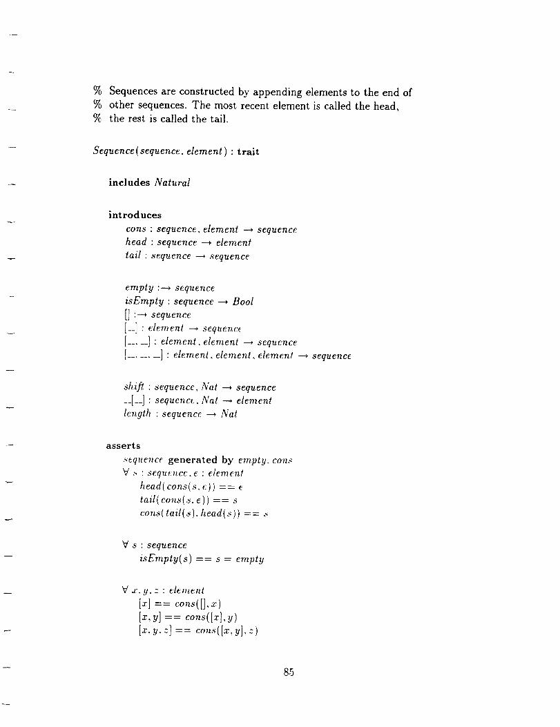
% Sequencesare constructed by appendingelementsto the end of

% other sequences. The most recent element is called the head,

% the rest is called the tail.

Sequence(sequence, element ) : trait

includes Natural

introduces

cons : sequence, element ---+sequence

head : sequence --+ element

tail : sequence _ sequence

empty :---+ sequence

isEmpty : sequence ---, Bool

[] :--+sequence[__]: element ---+ sequence

[..... ]: element, element ---+sequence

[........ ] : element, element, element ---+sequence

shift :sequence, Nat _ sequence

__[__]:sequence, Nat _ element

length :sequence ---, Nat

asserts

.,equence generated by empty, coT_s

V .4 : sequence, e : element

head(cons(s, e)) == e

tail(cons(s, e)) == _

cons( tail(.s ). head(5)) = =.,

_/ S : sequence

isEmpty(s) == s = empty

V x. g. z : elemenl

Ix] == cons([],.'_:/Ix, y] == cons([z],y)[x,y. :] == cons(Ix,y],:)

85

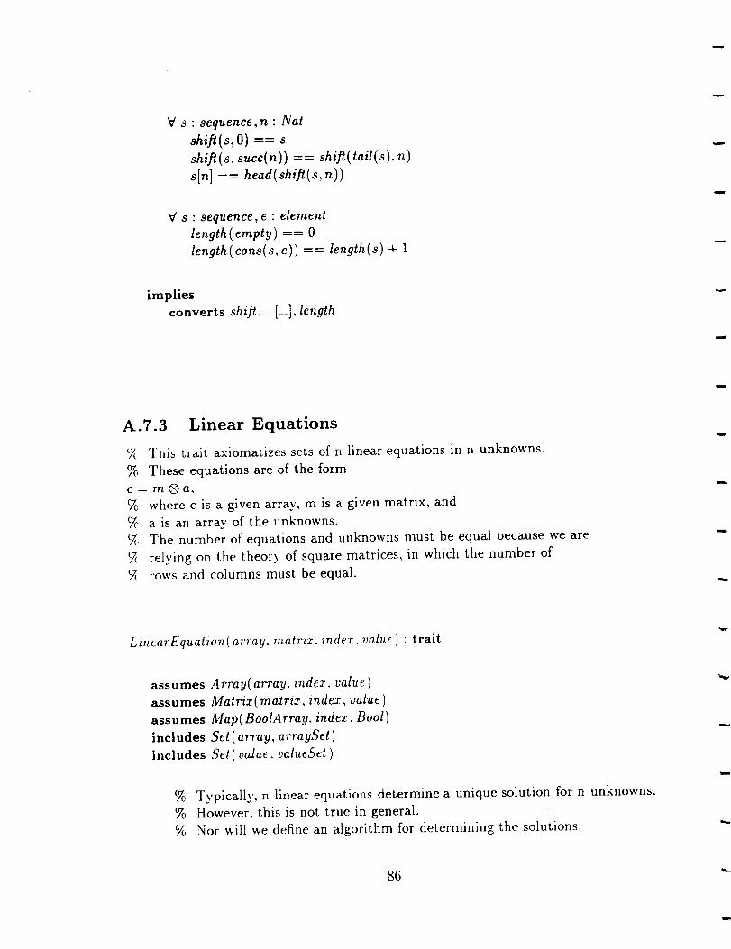
V s : sequence, n : Nat

shift(s, O) == s

shift(s, succ(n) ) == shift( tail( s ), n )

s[n] == head(shift(s,n))

V s : sequence, e : element

length (empty) == 0

length(cons(s, e)) == length(s) + 1

implies

converts shift, __[__], length

A.7.3 Linear Equations

tX Tills trait axiomatizes sets of n linear equations in n unknowns.

These equations are of the form

C ---- VI2 _ a ,

% where c is a given array, m is a given matrix, and

a is an array of the unknowns.

t2_ The number of equations and unknowns must be equal because we are

7( relying on the theory of square matrices, in which the number of

rows and columns must be equal.

L_,earEquation( array, matrix, index, value) : trait

assumes Array(array, index, value )

assumes Matrix(matrix, index, value )

assumes Map( BoolA tray, index, Bool)

includes Set ( array, arraySet )

includes Set ( value, valueSet )

% Typically, n linear equations determine a unique solution for n unknowns.

% However, this is not true in general.

_, Nor will we define an algorithm for determining the solutions.

86

% Rather, we describe the properties every set of solutions must have,

% and the dependence of each unknown on the input array c.

%introduces

solutions and sets of solutions.

solutions : array, matrix _ arraySet

solutions : arraySet, matrix --* arraySet

solve : array, matrix _ array

_7( If BoolArray indicates which components of input array c are fixed,

_ determine indicates which components of unknown array a are determined.

determine : BoolArray, array, matrix --_ BoolArray

% arrays match at components where BoolArray is true.

match : BoolArray, array, array _ Bool

_, set of arrays matching at BoolArray.

matches : BoolArray, array _ arraySet

% the set of values of a given array component

__[__] : arraySet, iT_dex _ valueSet

% uniqueness for each array component

unique : arraySet ---, BoolArray

asserts

V m : matrix, a. c : array, s : arraySet

a E solutions(c,m)==m@a=c

a E solutions(s,m) == (m ® a) E s

solve(c, rn) C solutions(c, m)

V b : BoolArray, c: array, ra : matrix

determine(b, c, m) --

unique (solutions ( match es( b, c), m) )

V b : BooIArray, a, c : array, i : index

match(b,a,c) --

- 87

b[i] = c[i]a E matches(b, c) ==

match(b, a, c)

_/ s : awaySet, a : array, i • index

(1})ill = {}insert(s, a)[i] == insert( s[i], a[i])

V s : arraySet, i : index

unique(s)[i] == size(s[i])= 1

A.7.4 Arrays and Matrices

An array is a map from an index sort to a value sort,

% where the value sort is a field.

The field requirement allows us to describe vector-like operations,

% such as inner product.

However. arrays are not vectors, because coordinates and coordinate

'7_ transformations have not been specified.

Array(array, index, value ) ' trait

includes Map( array, index, value )

assumes Field( value. +. *)

introduces

: array --+ value

__ + __ : array, array ---* array

• : array, array---* array

__ • __ : array, array ---* value

• : value, array --* array

• : array, value ---* array

-__ : array --* array

unit : index --* array

0 :--_ array

%

%

sum of array components

% component-wise sum

component-wise product

% inner product

% left scalar product

% right scalar product

% negation

% unit vector

% a constant

I

i

88 "

asserts

V al, as : array, i : index

(a, + a2)[i] == al[i] + as[i]

(a, • a2)[i] == al[i] * as[i]

al "as == _'(al * as)

V c : value, a : array, i : index

(c• a)[i] == c • a[i](a,c)[i]==c,a[i]

-a == (-1) * a

V i,j : index

unit(i)[j] --

ifi=j then 1 else0

0[j] == 0

The sigma operator is not converted because nothing is yet specifiedabout the index sort to be summed over.

implies

converts __ + __ : array, array ---* array,

__ * __ : array, array ---* array,

• : value, array --* array,

• : array, value --_ array,

-__ : array --_ array,

, unit,

0 :--_ array

89

% A matrix is a map from an element,which is a pair of indices,% to a value, where the possiblevaluesform a field.% Becausewe haveusedthe sameindex sort for both componentsof the pair,% weare axiomatizing squarematricesonly.

Matrix(matrix, index, value ) : trait

assumes Array( array, index, value)

element tuple of row, column : index

includes Map( matrix, element, value)

introduces

row : matrix, index _ array

column : matrix, index _ array

__ + __ : matrix, matrix _ matrix

• : value, matrix _ matrix

• : matrix, value _ matrix

__ _' __ : matrix, matrix _ matrix

--:5 -- : matrix, array _ array

__ ® __ : array, matrix _ array

O. 1 :---_ matrix

%% index by row arrays

index by column arrays

% component-wise sum

% left scalar product

% right scalar product

0_ multiplication

% right multiplication

% left multiplication

% constants

asserts

77z.m1,m 2 : matrix,a : array, e : element,i: index,c: value

,,,[_]== row(,,,,e.row)[e.colum,]-_[d := colum.(m.e.column)[e.row](._, + .,_)[e] := m,[_]+ m_[e](,,,, _ ,,_)[e]== ,'o_(m,,e.row).

column(m2, e.column )

(c *,_)[e]== c *m[e](m, c)[e]== c* m[e](m Q _)[i1== ,.ow(m,i).a(a ® m)[il == a. column(re, i)O[e]== 0lie] == if e.row = e.column then 1 else 0

implies

Field(matrix, +, C,)

90

converts row, column,

0 :---* matrix,

1 :---* matrix,

__ + __ : matrix, matrix --, matrix,

__ * _ : matrix, value ---, matrix,

-- * __ : value, matrix ---, matrix,

__ ® __ : matrix, array ---, array,

__ ® __ : array, matrix _ array,

__ ® __ : matrix, matrix ---* matrix

A.7.5 Registers

% A register is a finite sequence of bits.

% It is often interpreted as a natural number value, signed or unsigned.

% Note that bits in a register are numbered here starting with 0.

Resister (width) : trait

includes Map(register, Nat, Bool)

includes Natural

interval tuple of

base :Nat,

offset:Nat

introduces

width :---, l\: at % the number of bits in the register

% Define the unsigned value of a register,

% and of a interval of consecutive bits within the register.

value : register ---, Nat

value : register, interval _ Nat

% auxiliary functions.

inlnterval : Nat, interval _ Bool

allZelvs : registeT.---, Bool

allOnes : register ---, Bool

91

asserts

V r : register, n, m : Nat

value(r) == value(r, [0, width])

value(r, [n, _ucc(m)])==( if r[n + m] then 2"m else 0)+

value(v, [n, m])

value(r,[,',,0]) == 0

V n" Nat.i: interval

inlnterval(n, i) == i.base < n A (n < (i.base + i.offset))

V r : register, n : Nat

i,dut, vval(,,, [0, width])

(aUZero_(r)_ -_r[_])inlnterval (n, [0, width])

(aUOn_._(r)_ r[.])

A.7.6 Mappings

Tile GCS specification has man)' sorts that map one sort into another.

_2_ In each case. the following trait will be included.

Alap( map. domain, range) • trait

introduces

__[__] : map, domain _ range

asserts

map partitioned by __[__]

92

A.7.7 Statistics

% The statistics trait defines statistical properties of collections of Reals.

% These properties are used in the ASP trait.

% We also introduce some convenient notation for bags of Reals.

Statistics : trait

includes Real

includes Bag(Real, RealBag, Nat for Card)

introduces

sum : RealBag _ Real

mean : RealBag ---, Real

varianceSum : RealBag _ Real

variance : RealBag _ Real

standardDeviation : ReaIBag ---* Real

%

% sum of bag elements

% mean of bag elements

sum of squared deviations

% mean-square

% root-mean-square

{ ..... } :Real, Real--_ ReaIBag

{..... , __} : Real. Real, Real _ ReaIBag

{ ........... } : Real, Real, Real, Real _ RealBag

asserts

V b: RealBa9,7" : Real

sum({})==O

sum(insert(b,,')) == r + sum(b)

mean(b) == su m ( b) / nat To R eal ( size ( b) )

This definition of variance is slightly different than the usual

% (for a finite sample, should use size(b)-i rather than size(b)),

% but it is the one required in SR.

varia, ceSum({ }) == 0varianceSum ( insert( b, r )) --

((r - mean(b))A2) + varianceSum(b)

variance(b) = varianceSum (b)/ nat ToReal( size( b) )

standardDeviation (b) = = root (2, variance (b) )

V w,x,y,z : Real

{w,x} == insert( {w},x)

{w,x.y} == insert({w.x},U)

93

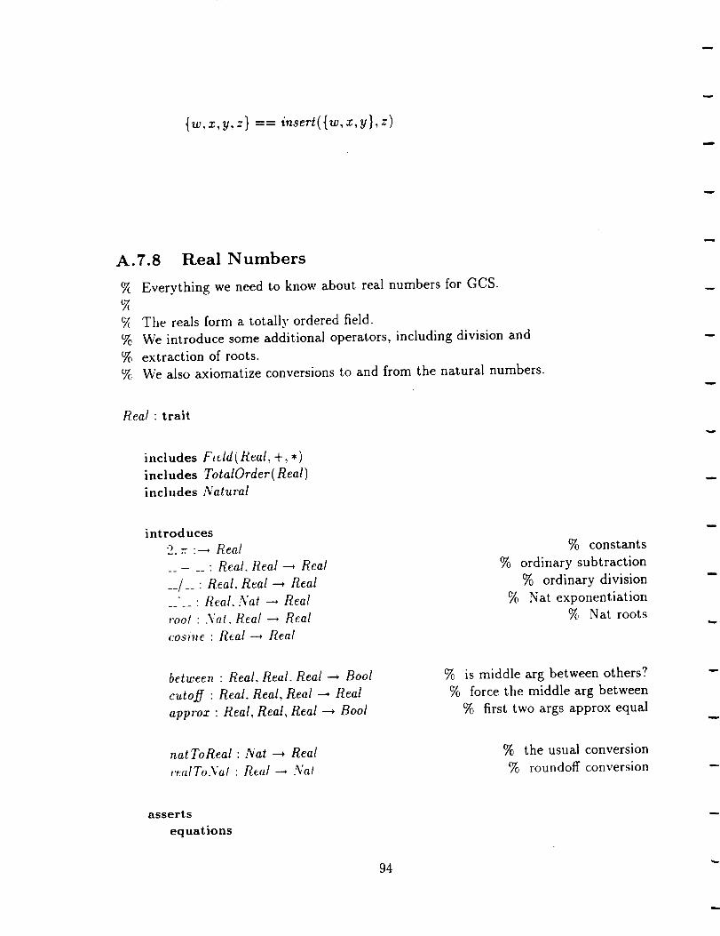
{w,x,y,z} == inse t({w,x, }, z)

A.7.8 Real Numbers

Everything we need to know about real numbers for GCS.

The reals form a totally ordered field.

% We introduce some additional operators, including division and

% extraction of roots.

% We also axiomatize conversions to and from the natural numbers.

Real: trait

includes Ficld( Real, +, *)

includes TotalOrder( Real)

includes Natural

introduces

2. _, :'--' Real

- __ : Real. Real _ Real

__/__ : Real, Real ---* Real

.... : Real. Nat _ Real

root : Nat. Real _ Real

cosine:Real--* Real

% constants

% ordinary subtraction

% ordinary division

% Nat exponentiation

_, Nat roots

between : Real, Real. Real--* Bool

cutoff : Real, Real, Real _ Real

approx : Real, Real, Real --_ Bool

% is middle arg between others?

% force the middle arg between

% first two args approx equal

nat ToReal: Nat --* Real

realToNal : Real _ Nat

% the usual conversion

% roundoff conversion

asserts

equations

94

O" Real < 1 • Real

2:Real== 1+1

V p, q, r : Real

p<q==(p+r)< (q+r)

P - q == P + (-q)

q # O_ (p/q)*q=p

q ¢ O _ (p , q)/q = p

V p: Real. n : Nat

p'O== 1

p'succ(n) == p. (p'n)

p >_ 0 _ root(n,p)'n = p

p > 0 _ root(n,p'n) = p

V r. lo, hi • Real

between(lo.r, hi) == lo < r A r < hi

lo < hi

cutoff ( lo, r, hi) =

( if r < lo then to else if r > hi then hi else r)

V p. q, precision " Real

approx(p, q, precision) --

betweel_ ( q - precision, p, q + precision)

V n : Nat.r : Real

natToReal(O) == 0

IlatToReal(succ(7_)) == 1 + natToReal(7_)

real]bNat(r) = n --

(natToReal(_) - (1/2)) _ rA

7" < (natTbReal(7_) + (1/2))

implies

V r, lo, hi • Real

1o < hi _ between(to, cutoff(to,7", hi), hi)

converts - • Real, Real ---* Real.

• " Real, Nat ---* Real.

between • Real. Real, Real _ Bool,

nat ToReal

95

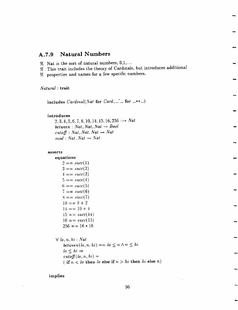
A.7.9 Natural Numbers

% Nat is the sort of natural numbers, 0,1,....

% This trait includes the theory of Cardinals, but introduces additional

% properties and names for a few specific numbers.

Natural : trait

includes Cardinal(Nat for Card, " for __**__)

introd uces

2, 3, 4, 5, 6, 7, 8, 10, 14, 15, 16,256 "--* Nat

between : Nat, Nat, Nat --* Bool

cutoff" Nat, Nat, Nat --* Nat

rood" Nat. Nat --* Nat

asserts

equations

2 == succ(1)3 == succ(2)

4 == succ(3)

5 =-= succ(4)

6 == succ(5)7 == succ(6)

8 == succ(7)t0 == S + '2

14 == 10+4

15 == succ(14)

16 == suet(15)

256== 16.16

V lo,n, hi • Nat

between(lo, n, hi) == 1o <_ n A 77 <_ hi

lo < hi

cutoff ( lo, n, hi) =

( if n < lo then lo else if n > hi then hi else n)

implies

96

AbelianSemigroup( Nat, +),

AbelianSemigroup( Nat, ,),

Distributive(Nat for T)

97

Appendix B

Critique of the Informal GCS

Requirements

NASA's Guidance and Control Software (GCS) experiment is a study of software de-

velopment methods. As part of this experiment, Research Triangle Institute (RTI)

wrote all informal software requirements document for GCS. This document is titled

"'Software Requirements: Guidance and Control Software Development Specification",

and was released in June 1990 [7]. We will refer to this document as "SR" throughout

this chapter.

ORA Corporation has written a formal specification for GCS, based on the infor-

mation in SR. This formal specification appears in Appendix A.

In the process of writing the formal specification we noted some problems, both

potential and actual, with the SR specification. This document lists the problems

noted. Most of the details in SR are in its descriptions of the functionality of each GCS

module. We devote one section here to each module in which problems were noted. The

first section, though, discusses a few problems found in the overall GCS requirements.

B.1 General Requirements

Several problems arise in SR's general requirements for GCS. Of these, the most im-

portant are the following:

• SR provides too much detail when stating the GCS requirements on functionality

and timing. In particular, it describes intermediate variables to be used in the

code. a decomposilion of the functionality into modules, and gives not only an

overall timing requirement but timing constraints for each module and a schedule

98

for activating modules. This detail makes SR essentially a software design, rather

than merely an expression of requirements.

• SR provides too little detail about the requirements on precision of computations.

In section 3.3 we place these problems within the context of a larger discussion ofrequirements specification for control software. We do not discuss them further here.

More specific problems follow:

Page 12's description of the GCS control needs to be updated: according to the

specification for AECLP, proportional-integral-derivative (PID) control is used

for pitch and yaw.

The data flow diagram on page 26 does not reflect all the flows actually required by

the rest of the specification. For example, ATMOSPHERIC_TF__P and AR_ALTITUDE

are both part of the SEI_SOR_0UTPUT data, according to the data dictionary. But

both serve as inputs to at least one of the sensor processing modules. Inputs to

sensor processing other than from the sensors themselves are not shown in the

data flow diagram.

B.2 AECLP

S1R's requirements for Axial Engine Control Law Processing (AECLP) have these prob-lems:

Table 5.2 defines pitch and yaw using different conventions: if pitch in this table

is right-handed, then yaw is left-handed, or vice-versa. This discrepancy is not

important if tile PID coefficients are chosen with the correct sign. but the signs

of these coefficients are also questionable (see next item).

There are nine PID coefficients in Table 5.2. The data dictionary requires (;AX to

be positive, but allows the other eight to have either sign. However, SR explicitly

negates another of these, (lB., thus suggesting that the coefficients will be chosen

positive.

One would expect that the three coefficients in each of the PID control laws would

have the same sign. The P and I terms are restoring forces, proportional to the

error and its integral, respectively. The D term damps oscillations, and should

therefore add to the P and I terms when the motion is increasing the error.

Therefore the negative sign modifying the GR term is either wrong or superfluous.

99

• In the control law for thrust, the purpose of the GAX term, not just its sign,

is questionable. As written, the term tends to be de-stabilizing: the greater

the downward acceleration, the faster the downward thrust decreases, leading to

greater downward acceleration. (This conclusion depends on the fact that the

data dictionary requires GA to be positive.) Therefore successful control must

depend on a choice of coefficients that makes the GVE and GVEI terms more

important than the GAX term in correcting deviations from the intended flight

path.

A term such as the GAX term is still needed, though, to determine the magnitude

of thrust in the absence of deviations from the intended flight path. Why should

this term depend on the measured acceleration in the lander's frame of reference?

Would it not be better to replace the GAX term with a function of altitude and

attitude approximating the thrust needed, e.g., a term proportional to

9rarity/cocO + dxJdt d(contour)/d(altitude)

where 0 is the angle between the verticals in the lander's and planet's coordinates,

and contour is the precomputed velocity-altitude contour?

• The data dictionary's description of OMEGA. "'gain of angular velocity", is wrong.

0MEGA's intuitive physical significance is the reciprocal of the time scale over which

changes in thrust are integrated.

• The matrix equation on page 36 that determines INTERNAL_CMD is inconsistent

with the diagram of the lander on page 9. SR does not say how the three axial

engines are numbered, but it does not matter: pitch control, according to the

equation, uses all three engines, but according to the diagram it depends on only

two: yaw control, according to the equation, uses two engines only, but according

to the diagram it must use all three. Obviously pitch and yaw are interchanged

here.

• Tile equation for INTERNAL_CMD also suggests a problem with signs. As written,

GPl and GP2 must have opposite signs so that they supply torque but not net

thrust. The data dictionary does not rule out this possibility, but the specifier

could have chosen, based on tile picture on page 9, to make all the constants in

this equation positive.

• AE_STATUS should be deleted from the specification. There are no stated condi-

tions under which it is given a value other than "healthy".

100

B.3 ARSP

SR's requirements for Altitude Radar Sensor Processing (ARSP) are unambiguous, but

the assumptions that seem to underlie those requirements are questionable.

If AR does not receive a radar echo in the current frame, it fits a cubic polynomial

to the previous four altitude values. Two questions arise:

Why are four values used? Using more values increases the probability of using

some that are unreliable (i.e., themselves based on extrapolation). Using fewer

values may decrease the precision of the extrapolation. Using fewer values sim-

plifies fitting, and therefore makes real-time deadlines easier to meet. So there

is a trade-off, and perhaps four values are optimal. SR does not provide enough

information to decide.

Why is a cubic fit to the four values? Using a cubic suggests that the first three

derivatives of altitude are non-negligible over four frames. But in acceleration

processing (ASP), the third derivative is assumed to be negligible in extrapolating

acceleration values. ASP's extrapolation is sometimes used in guidance processing

to get new values of velocitv and altitude, so precision is no less important in ASP

than ARSP.

Therefore fitting a quadratic to the altitude values is probably better than fitting

a cubic.

If the first and second derivatives are non-negligible, then why not use the values

for these from guidance processing (GP) to constrain the ARSP fit, rather than

letting the fit determine thenf? The result of this constrained fit, an altitude, is

likely to be more precise than the guidance processing value for altitude, because

the constrained fit uses several recent direct measurements of altitude rather than

the single most recent value used in GP.

Whether to make better use of available data to get a more precise value for

altitude is a decision that depends on GCS's specific requirements on precision.

These requirements are not, stated in SR.

B.4 ASP

SR's requirements for Accelerometer Sensor Processing (ASP) have the following prob-

lems:

• The requirement for converting raw counter data to an acceleration value seems

to contradict itself. First SR sas's: "The sign of the counter will always be posi-

101

tive, but the offset given in A_BIAS will be negative or zero, so if the magnitude

in A_C0UNTEK is smaller than that of A_BIAS, the acceleration is negative." To re-

inforce this, SR says: "Each accelerometer has a characteristic DC bias (A_BIAS)

which must be removed from the signal prior to conversion." Both statements

suggest a conversion of the form

acceleration = gain * (A_COUNTER + A_BIAS)

SR also says, however: "The acceleration is a linear function of its A_COUNTE.R

value where the gain specifies the slope and the offset (A_BIAS) specifies the inter-

cept." To reinforce this, SR writes an equation for converting each acceleration

component:

acceleration = A_.BIAS + gain * A_COUNTER

Which is right? The GCS formal specification uses the second interpretation.

• The misalignment correction is wrong. SR defines an ALPHA_MATRIX of small

correction angles, and defines the small angles in the adjacent text. The matrix

shown, however, must be transposed and the alphas negated in order to follow

the text.

• The sample standard deviation is defined incorrectly. The definition is the stan-

dard deviation of the parent distribution, which will differ from the sample stan-

dard deviation unless the mean is known with perfect accuracy (which is not the

case here).

• The algorithm for eliminating flaky acceleration values is questionable. Its intent

seems to be that an acceleration value is unreliable ("unhealthy") if it is too far

from the mean of recent values. However, if the mean itself depends on unreliable

values, then the algorithm forces the current value to be reliable. If we suppose the

reliability of each measurement to be independent of the others, this algorithm is

absurd: the current value becomes more reliable simply because its predecessors

are less so.

A better approach almost certainly exists. Why is a mean of recent measure-

ments used instead of a more complicated extrapolation? Presumably because

the change in acceleration over four frames is negligible. Why is a mean taken

for just three measurements? Presumably because the probability of flaky values

is small enough that getting two of them in four consecutive frames is unlikely.

So why not take the mean of the three most recent reliable values? This will

almost never need more than one additional previous frame, and the change in

acceleration over five frames is probably still negligible.

Justifying an alternate approach, of course, demands an understanding of the

detailed dynamics and of the sensor precision. These details are not available in

SR.

102

B.5 CP

SR's requirements on Communications Processing (CP) have these problems:

• On page 46, SR notes that the diagonal terms of G_ROTATION should not be

sent. G_ROTATION is a history of vectors, so there are no diagonal terms to

send. Probably the reference should be to GP_ROTATION, whose diagonal terms

are always zero. However, GP_ROTATION should not be sent at all, because it is

essentialh an intermediate variable determined entirely by 6_ROTATION.

This mistake, though minor, is but the tip of an iceberg. Generally. SR should

not be listing the variables to send because specific decision about GCS's data

structures should be at the discretion of the programmer. Some of the "variables"

listed in CP, such as GP_ROTATION, might not even exist in the implementation.

This general problem of overspecification is discussed in chapter 3

• C_STATUS should be deleted from the specification. There are no stated conditions

under which it is given a value other than "healthy". And even if C_STATUS did

depend on whether CP was working OK. there would be no reason to transmit

it as part of a communication packet: the arrival of uncorrupted packets shouldbe the best indication of CP's health.

B.6 GSP

SR's requirement on Gyroscope Sensor Processing (GSP) seems to contradict itself.

The raw sensor data for each axis is a counter that holds both a sign bit and a 14

1,ii ,_mg,Jitudc. Tlu. rex1 describes the conversion: "Tile rotation rate is linear with

respect to tile unprocessed gyroscope values, i.e.. the lower 14 bits must be converted."

Therefore. when the sense of the rotation is included, the conversion should be written

rotatioTt = sign(counter) • (offset + gain • magnitude(counter))

But SR goes on to write the conversion as

rotation = offset + gain • counter

Which is right?

The GCS formal specification uses the former interpretation.

(]_STATUS should be deleted from the specification. There are no stated conditions

under which it is given a value other than "healthy".

103

B.7 GP

SR's requirements for Guidance Processing (GP) have these problems:

• The equation on page 54 for the derivative of dynamical quantities is wrong. To

see this, note that it is dimensionally incorrect in the case of velocity: the left hand

side has dimensions of an acceleration, but the right hand side correction term

has dimensions of a velocity. The problem could be fixed by using a difference

equation instead, e.g.,

A(variable) = a x variableAt + BAt + correction _errn

However. this fix effectively requires Euler integration, while SR explicitly allows

better integration algorithms to be used in this case.

A better fix would be to eliminate the correction terms and replace them with

conditionals in the specification logic (see next item).

• The terms with the K_ALT and K_MATRIX factors are misleadingly called "correc-

tion terms". Their real purpose is to choose measured values from ARSP and

TDLRSP if they are reliable, or choose values gotten by integration in GP oth-

erwise. It woulc] be better to state this requirement explicitly, than to embed it

as a kludge in equations for the lander's dynamics.

B.8 RECLP

RE_STATUS should be deleted from the specification.

under which i_ is given a value other than "healthy".

There are no stated conditions

B.9 TDLRSP

SR's requirements on Touch Down Landing Radar Sensor Processing (TDLRSP) are

unambiguous, but this fact only becomes clear after making an educated guess about

the intentions behind the requirements and re-deriving the "requirements" from the

intentions. The document would be much clearer if either

• it gave a few more clues about the intentions, or

• the intentions were stated as the requirements, and the software engineer were

allowed to derive consequences from them.

104

The formal requirements specification for GCS follows the latter course. This course

has two advantages:

1. The requirements are more abstract, and as a result are more easily adapted if

the design of the spacecraft changes.

2. The programmer reading the requirements is not left guessing.

To understand the problem, compare Figure 5.4 on page 69 with Figure 5.3 on page

66. Figure 5.3 shows the directions of the four radar beams, while Figure 5.4 names

the direction cosines for the beam in the first octant. The programmer is expected

to realize that the directions of the other three beams are also gotten from the same

direction cosines. But how? Reflection in the coordinate planes? Rotation through

90 degrees? Other? Only after re-deriving the expressions in Table 5.10 can one be

sure that it must be reflection, because only in that case will the values of two beams

uniquely determine one component of the velocity.

SR's figure 5.3 does suggest that the beam directions determine a rectangle, centered

on the origin, and parallel to the coordinate axes. SR should at least make this explicit.

The intentions behind the requirements can be stated much more succinctly than

Table 5.10: use every available beam measurement to determine as many components

of the velocity as possible. If a component of the velocity is underdetermined, flag

its value as t, nreliable. If a component of the velocity is overdetermined, average thevalues gotten from the different sets of beam measurements that determine it.

SR does not make clear why this intention is good enough. If in some frame only

two beam measurements are available, exactly one velocity component is determined.

The other components are gotten from Guidance Processing (GP) by integrating the

acceleration. These GP components are considered less reliable because they are not

gotten from direct measurement. But this method wastes tile more precise information

available in TDLR's direct Ineasurement: two measurements should determine two

degrees of freedom, not just one. Why' isn't the GP information averaged with the

TDLR measurement, weighted by the relative precision of the two? This averaging

would yield a more precise value of velocity in this case.

Finally', TDLR_STATUS should be deleted from the specification. There are no stated

conditions under which it is given a value other than "healthy".

B.IO TSP

._R'_ I'equivemeuts on Temperature Sensor Processing (TSP) have the following prob-lenls:

105

• Paragraph 1 is misleading. The requirements on TSP are intended to maximize

the precision of measurements; the effect on the accuracy depends on random

factors in each measurement. The thermocouple pair sensor is more precise in

the range for which its calibration gives accurate results; the solid-state sensor

gives accurate results over a wider range.

• The requirements on the calibration of the thermocouple pair appear incomplete.

The thermocouple pair is calibrated by a parabola near the ends of its usable

range. SR states requirements that determine these parabolas. One of the require-

ments is "The upper (and lower) parabolas are defined so that the temperature

goes up (or down) as the square of the measurement value." Evidently (T- To) =

a(M -M0) 2, where To and M0 are to be determined by the two other requirements

given in SR. Are we to assume that a = +ldegree Centigrade/count-_2?

This is the only instance in SR where a dimensional constant used in sensor

calibration is not specified in the data dictionary, and not loaded at GCS ini-

tialization. Perhaps neglecting o is a side-effect of simplifying the Viking lander

software to become GCS.

This neglect may not turn into a problem, because it is unlikely the dimensions

chosen for temperature will be changed during the design process. However, the

specification of TSP is not invariant under such changes.

• The requirement on when to use the thermocouple pair is certainly wrong. SR

states "If the temperature derived from SS_TEMP falls within the accurate tem-

perature response zone of the thermocouple pair, ..., then the value returned by

the thermocouple pair should be used;..." This suggests the solid-state sensor

temperature must be calculated first, then a decision made based on the result

of the measurement. There are two reasons not to do this:

.

"2.

SR specifies elsewhere that the thermocouple pair is calibrated accurately

over a certain range of raw sensor readings, not over a range of temperature.

Even if we use the thermocouple's calibration to convert the range of sensor

readings into a range of temperatures, it is still better to decide which sensor

to use based on the raw readings. Every measurement is imprecise, espe-

cialh' those of the solid-state sensor. Therefore, it is possible for the raw

sensor readings to fall outside the thermocouple pair's range of accuracy,

but for the solid-state sensor to convert the raw readings into a temperature

value apparently inside the range. Converting the thermocouple pair's read-

ing could then yield an inaccurate result. The likelihood of this occurring

depends on the imprecision of the solid-state sensor.

• TS_STATUS should be deleted from the specification. There are no stated condi-

tions under which it is given a value other than "health)'".

106

B.11 Data Dictionary

There are several trivial mistakes in the Data Dictionary which should be fixed if a

new requirements document is produced.

• AE_TEMP has three values, so its data type cannot be logical*l.

• The dimension radians is used in various places in the data dictionary, including

for TDLR_ANGLES, so it should also be used for the angles in ALPHA_MATRIX.

• How could FRAME_COUNTER be EXTERNAL?

• The descriptionof G_0FFSET uses the name ROTATION_RAW, which does not appear

elsewhere in the dictionary.

• RE_SWITCH isalso used in RECLP.

107

Bibliography

[1] Philip R. Bevington. Data Reduction and Error Analysis for the Physical Sciences.

McGraw-Hill. 1969.

[2] Robert S. Boyer, Milton W. Green, and J Strother Moore. The use of a formal

simulator to verify a simple real time control program. In Beauty is Our Business.

Springer-Verlag, 1990.

[3] Software considerations in airborne systems and equipment certification (DO-178-

B.5). RTCA paper no. 591-91/SC167-164. November 1991. 1140 Connecticut Av-

enue. N\¥. Suite 1020. Washington. DC 20036.

[4] Janet R. Dunham. Experiments in software reliability: Life-critical applications.IEEE Transactions on Software Engineering: Special Issue on Software Reliability,

January' 1986.

[5] David Guaspari. Carla Marceau, and Wolfgang Polak. Formal verification of Ada

programs. IEEE Transactions on Software Engineering, 16:1058-1075, September

1990.

[6] .lohn V. Guttag. James ,]. Horning. and Andres Modet. Report on the larch shared

language: Version 2.3. Technical report. Digital Equipment Corp. Systems Research

(;enter. April 1990.

[7] B. Edward Withers et al. Software requirements: Guidance and control software

development specification. Technical report, Research Triangle Institute, June 1990.

108

Form ApprovedREPORT DOCUMENTATION PAGE OMBNo. 0704-0188

gaff,wingand m_nmlnw_ l,m 0_i mlqldlCL ind c_n_ololr_ .I_ rlvNw_0 I_i .a)N_jon. o( _ Sor_l_c_nwn_l rl_l_g _,_sl_in ostmlm _'.any ome__.Isi_l_..oIm_s

H_nvmy, S_e 1204./ulm_on.VA 222_..4302,end to_ 0_ olMana_me_ and _ _ R_XJm_onPro_c_l_r/o4.01U],Wa_'ungmn,DC 20503

1. AGENCY USE ONLY (Leave blank) :L REPORT DATE 3. REPORT TYPE AND DATES COVERED

April 5, 1994 Contractor Report4. TITLE AND SUBTITLE 5. FUNDING NUMBERS

Using Formal Specification in the Guidance and Control Software (GCS)Experiment

6. AUTHOR(S)

Doug Weber and Damir Jamsek

7. PERFORMING ORGANIZATION NAME(S) AND ADDRESS(ES)

Odyssey Research Associates301 Dates Drive

Ithaca, NY 14850-1326

9. SPONSORING I MONITORING AGENCY NAME(S) AND ADDRESS(F.S)

National Aeronautics and Space AdministrationLangley Research CenterHampton, VA 23681-0001

C NAS1-18972

WU 505-64-10-51

8. PERFORMING ORGANIZATIONREPORT NUMBER

TM-92-0046

I10. SPONSORING/MONITORINGAGENCY REPORT NUMBER

NASA CR-194884

11.SUPPLEMENTARYNOTES

Task 7 ReportLangley Technical Monitor: Sally C. Johnson

12a. DISTRIBUTION I AVAILABILITY STATEMENT

Unclassified - Unlimited

Subject Category 60

12b. DISTRIBUTION CODE

13. ABSTRACT (Maximum 200 words)

The goal of this task was to investigate how formal methods could be incorporated into a software engineeringprocess for flight-control systems under DO-178B and to demonstrate that process by developing a formalspecification for NASA's Guidance and Controls Software (GCS) Experiment. GCS is software to control thedescent of a spacecraft onto a planet's surface. The GCS example is simplified from a real example spacecraft,but exhibits the characteristics of realistic spacecraft control software. The formal specification is written inLarch.

14. SUBJECT TERMS

Formal Methods, Specification,Guidance and Controls

17. SECURITY CLASSIFICATION

OF REPORT

Unclassified

18. SECURITY CLASSIFICATIONOF THIS PAGE

Unclassified

19. SECURITY CLASSIFICATIONOF ABSTRACT

15. NUMBER OF PAGES

108

16. PRICE CODE

20. LIMITATION OF ABSTRACT