SOFTWARE SPECIFICATION: A Comparison of Formal Methods
259
SOFTWARE SPECIFICATION: A Comparison of Formal Methods by John D. Gannon, James M. Purtilo, Marvin V. Zelkowitz Department of Computer Science University of Maryland College Park, Maryland February 23, 2001 Copyright c 1993
Transcript of SOFTWARE SPECIFICATION: A Comparison of Formal Methods
SOFTWARE SPECIFICATION:
A Comparison of Formal Methods
byJohn D. Gannon, James M. Purtilo, Marvin V. Zelkowitz
Department of Computer ScienceUniversity of MarylandCollege Park, Maryland
February 23, 2001
Copyright c�1993
Contents
Preface ix
1 Introduction 11. A HISTORICAL PERSPECTIVE � � � � � � � � � � � � � � 5
1.1. Syntax � � � � � � � � � � � � � � � � � � � � � � � � � 51.2. Testing � � � � � � � � � � � � � � � � � � � � � � � � � 61.3. Attribute Grammars � � � � � � � � � � � � � � � � � 71.4. Program Verification � � � � � � � � � � � � � � � � � 7
2. A BRIEF SURVEY OF TECHNIQUES � � � � � � � � � � � 92.1. Axiomatic Verification � � � � � � � � � � � � � � � � 92.2. Algebraic Specification � � � � � � � � � � � � � � � � 102.3. Storage � � � � � � � � � � � � � � � � � � � � � � � � � 112.4. Functional Correctness � � � � � � � � � � � � � � � � 132.5. Operational Semantics � � � � � � � � � � � � � � � � 13
3. SEMANTICS VERSUS SPECIFICATIONS � � � � � � � � 154. LIMITATIONS OF FORMAL SYSTEMS � � � � � � � � � � 165. PROPOSITIONAL CALCULUS � � � � � � � � � � � � � � � 17
5.1. Truth Tables � � � � � � � � � � � � � � � � � � � � � � 195.2. Inference Rules � � � � � � � � � � � � � � � � � � � � 195.3. Functions � � � � � � � � � � � � � � � � � � � � � � � � 215.4. Predicate Calculus � � � � � � � � � � � � � � � � � � 225.5. Quantifiers � � � � � � � � � � � � � � � � � � � � � � � 255.6. Example Inference System � � � � � � � � � � � � � � 26
6. EXERCISES � � � � � � � � � � � � � � � � � � � � � � � � � � 277. SUGGESTED READINGS � � � � � � � � � � � � � � � � � � 28
2 The Axiomatic Approach 311. PROGRAMMING LANGUAGE AXIOMS � � � � � � � � � 31
v
vi Software Specifications
1.1. Example: Integer Division � � � � � � � � � � � � � � 341.2. Program Termination � � � � � � � � � � � � � � � � � 381.3. Example: Multiplication � � � � � � � � � � � � � � � 381.4. Another Detailed Example: Fast Exponentiation � 421.5. Yet Another Detailed Example: Slow Multiplication 45
2. CHOOSING INVARIANTS � � � � � � � � � � � � � � � � � 473. ARRAY ASSIGNMENT � � � � � � � � � � � � � � � � � � � � 48
3.1. Example: Shifting Values in an Array � � � � � � � 503.2. Detailed Example: Reversing an Array � � � � � � 53
4. PROCEDURE CALL INFERENCE RULES � � � � � � � � 574.1. Invocation � � � � � � � � � � � � � � � � � � � � � � � 584.2. Substitution � � � � � � � � � � � � � � � � � � � � � � 594.3. Adaptation � � � � � � � � � � � � � � � � � � � � � � � 624.4. Detailed Example: Simple Sums � � � � � � � � � � 664.5. Recursion in Procedure Calls � � � � � � � � � � � � 724.6. Example: Simple Recursion � � � � � � � � � � � � � 73
5. EXERCISES � � � � � � � � � � � � � � � � � � � � � � � � � � 756. SUGGESTED READINGS � � � � � � � � � � � � � � � � � � 84
3 Functional Correctness 851. PROGRAM SEMANTICS � � � � � � � � � � � � � � � � � � 862. SYMBOLIC EXECUTION � � � � � � � � � � � � � � � � � � 883. DESIGN RULES � � � � � � � � � � � � � � � � � � � � � � � 90
3.1. Design of Assignment Statements � � � � � � � � � 903.2. Design of Conditional Statements � � � � � � � � � 913.3. Verification of Assignment and Conditional State-
ments � � � � � � � � � � � � � � � � � � � � � � � � � � 924. SEMANTICS OF STATEMENTS � � � � � � � � � � � � � � 93
4.1. Begin Blocks � � � � � � � � � � � � � � � � � � � � � � 934.2. Assignment Statement � � � � � � � � � � � � � � � � 934.3. If Statement � � � � � � � � � � � � � � � � � � � � � � 944.4. While Statement � � � � � � � � � � � � � � � � � � � 94
5. USE OF FUNCTIONAL MODEL � � � � � � � � � � � � � � 985.1. Example: Verification � � � � � � � � � � � � � � � � � 985.2. Example: Design � � � � � � � � � � � � � � � � � � � 1035.3. Multiplication – Again � � � � � � � � � � � � � � � � 104
6. DATA ABSTRACTION DESIGN � � � � � � � � � � � � � � 1076.1. Data Abstractions � � � � � � � � � � � � � � � � � � � 1076.2. Representation Functions � � � � � � � � � � � � � � 108
7. USING FUNCTIONAL VERIFICATION � � � � � � � � � 1118. EXERCISES � � � � � � � � � � � � � � � � � � � � � � � � � � 1129. SUGGESTED READINGS � � � � � � � � � � � � � � � � � � 117
vii
4 Predicate Transformers 1191. GUARDED COMMANDS � � � � � � � � � � � � � � � � � � 119
1.1. Guarded If Statement � � � � � � � � � � � � � � � � 1201.2. Repetitive statement � � � � � � � � � � � � � � � � � 120
2. WEAKEST PRECONDITIONS � � � � � � � � � � � � � � � 1222.1. Axioms � � � � � � � � � � � � � � � � � � � � � � � � � 1222.2. If Statements � � � � � � � � � � � � � � � � � � � � � 1222.3. Do Statements � � � � � � � � � � � � � � � � � � � � � 125
3. USE OF WEAKEST PRECONDITIONS � � � � � � � � � � 1283.1. Example: Integer Division � � � � � � � � � � � � � � 1283.2. Still More Multiplication � � � � � � � � � � � � � � � 129
4. EXERCISES � � � � � � � � � � � � � � � � � � � � � � � � � � 1325. SUGGESTED READINGS � � � � � � � � � � � � � � � � � � 134
5 Algebraic Specifications 1371. MORE ABOUT DATA ABSTRACTIONS � � � � � � � � � � 1372. OPERATIONAL SPECIFICATIONS � � � � � � � � � � � � 1393. ALGEBRAIC SPECIFICATION OF ADTS � � � � � � � � 141
3.1. Developing Algebraic Axioms � � � � � � � � � � � � 1443.2. Hints For writing algebraic axioms � � � � � � � � � 1473.3. Consistency � � � � � � � � � � � � � � � � � � � � � � 1513.4. Term Equality � � � � � � � � � � � � � � � � � � � � � 152
4. DATA TYPE INDUCTION � � � � � � � � � � � � � � � � � � 1524.1. Example: Data Type Induction Proof � � � � � � � � 155
5. VERIFYING ADT IMPLEMENTATIONS � � � � � � � � � 1565.1. Verifying Operational Specifications � � � � � � � � 1565.2. Verifying Algebraic Specifications � � � � � � � � � � 1605.3. Example: Verifying an Implementation of Stacks 1625.4. Verifying Applications With ADTs � � � � � � � � � 1675.5. Example: Reversing an Array Using a Stack � � � 168
6. INDUCTIONLESS INDUCTION � � � � � � � � � � � � � � 1716.1. Knuth–Bendix Algorithm � � � � � � � � � � � � � � 1716.2. Application of Knuth Bendix to induction � � � � � 1766.3. Example Using Knuth–Bendix � � � � � � � � � � � 179
7. EXERCISES � � � � � � � � � � � � � � � � � � � � � � � � � � 1838. SUGGESTED READINGS � � � � � � � � � � � � � � � � � � 191
6 Denotational Semantics 1931. THE LAMBDA CALCULUS � � � � � � � � � � � � � � � � � 193
1.1. Boolean Values as �Expressions � � � � � � � � � � 1951.2. Integers � � � � � � � � � � � � � � � � � � � � � � � � � 196
viii Software Specifications
2. Datatypes � � � � � � � � � � � � � � � � � � � � � � � � � � � � 1972.1. Continuous Functions � � � � � � � � � � � � � � � � 1992.2. Continuity � � � � � � � � � � � � � � � � � � � � � � � 2002.3. Recursive Functions � � � � � � � � � � � � � � � � � 2012.4. Evaluation of FACT Function � � � � � � � � � � � � 203
3. PROGRAMMING SEMANTICS � � � � � � � � � � � � � � � 2033.1. The Simple Model � � � � � � � � � � � � � � � � � � � 2043.2. Pointers and Aliasing � � � � � � � � � � � � � � � � � 2093.3. Continuations � � � � � � � � � � � � � � � � � � � � � 210
4. EXERCISES � � � � � � � � � � � � � � � � � � � � � � � � � � 2125. SUGGESTED READINGS � � � � � � � � � � � � � � � � � � 213
7 Specification Models 2151. VIENNA DEVELOPMENT METHOD � � � � � � � � � � � 215
1.1. Overview of VDM � � � � � � � � � � � � � � � � � � � 2161.2. Example: Multiplication One Last Time � � � � � � 2201.3. Summary of VDM � � � � � � � � � � � � � � � � � � � 222
2. TEMPORAL LOGIC � � � � � � � � � � � � � � � � � � � � � 2232.1. Properties of Temporal Logics � � � � � � � � � � � � 2232.2. Programming Assertion � � � � � � � � � � � � � � � 228
3. RISK ANALYSIS � � � � � � � � � � � � � � � � � � � � � � � 2313.1. Decisions under Certainty � � � � � � � � � � � � � � 2313.2. Decisions under Uncertainty � � � � � � � � � � � � 2323.3. Risk Aversion � � � � � � � � � � � � � � � � � � � � � 2343.4. Value of Prototyping � � � � � � � � � � � � � � � � � 235
4. SUGGESTED READINGS � � � � � � � � � � � � � � � � � � 237
References 239
Author Index 245
Index 247
Preface ix
Preface
Formal methods help real programmers write good code.
Well, this is what we believe, anyway. Likewise, we believe verificationtechniques can scale up for use in large and realistic applications. Butleast you think we will next profess a belief in the tooth fairy or ‘nonew taxes’ as well, let us quickly acknowledge that the field has con-siderable engineering to do before industry will accept the economicsof treating software mathematically. Many different technologies mustbe developed and compared with one another, and their utility must beevaluated in realistic case studies.
But how to get this activity out of the campus labs and into the field?
Here at the Computer Science Department at the University of Mary-land, recognizing that a corps of formalism-trained researchers andpractitioners is necessary for specification technology to really see thegrowth it needs, we have focused our curriculum in software to stressthe importance of being able to reason about programs. This themeaffects our graduate and undergraduate programs alike, but it is theformer program that this book is all about.
What is this book about?
During the prehistoric era of computer technology (say, about 1970),formal methods centered on understanding programs. At this time,we created the graduate course CMSC 630: Theory of ProgrammingLanguages. The theme of the course was programming semantics, ex-plaining what each programming language statement meant. This wasthe era of the Vienna Definition Language, Algol-68 and denotationalsemantics. Over the next ten years, program verification, weakest pre-conditions, and axiomatic verification dominated the field as the goalchanged to showing that a program agreed with a formal description ofits specification. During the 1980s, software engineering concerns andthe ability to write a correct program from this formal specification fol-lowed. Our course kept evolving as the underlying technology changedand new models were presented. With all three models, however, thebasic problem has remained the same, showing that a program and itsformal description are equivalent. We now believe that this field hasmatured enough that a comprehensive book is possible.
x Software Specifications
How did we come to write this book?
Over the years that we have taught formal methods to graduate stu-dents, we found no one textbook that would compare the various meth-ods for reasoning about software. Certainly there are excellent books,but each deals in only a single approach, and the serious student whoseeks a comprehensive view of the field is faced with the task of track-ing down original journal papers, translating arcane notations, andmaking up his or her own sample problems. So the book you are read-ing now represents our effort to consolidate the available formalismsfor the purpose of detailed comparison and study.
This book started as a loose collection of handwritten notes by one ofus (Gannon), who sought to stabilize our graduate course in its earlyyears. These notes were cribbed and modified by many of the facultyat Maryland as they did their tour in front of the 630 classes. Oneday the second author (Purtilo) volunteered to teach 630, claiming thatafter years of writing good programs he thought it would be nice tobe able to demonstrate that they were correct; and so the notes werepassed to this wonderfully naive colleague. As an aid in learning thematerial before he had to teach it to the class, Purtilo was responsiblefor the initial cleanup and typesetting of the notes, and he expandedthe document over the course of several semesters. Finally, the noteswere passed to the third author (Zelkowitz). In needing to relearn thismaterial after not teaching the course for about five years, he expandedthe notes with new material and, with heroic efforts, repaired some ofthe second author’s proofs. This collection is what is presented heretoday.
Who should read this book?
The punch line is that this is material we have used extensively, hav-ing been tested on many generations of graduate students, to whomwe are greatly indebted for many excellent suggestions on organiza-tion, accuracy, and style. Of course, you don’t need to be a graduatestudent looking for a research topic to benefit from this book. Even ifyou don’t write code from a formal specification, we have found thatan understanding of which program structures are easier to manipu-late by formal techniques will still help you write programs that areeasier to reason about informally. The basic technology is useful inall programming environments and an intuitive understanding of thetechniques presented here are valuable for everyone.
Preface xi
Parts of Chapters 1, 3 and 6 are extensions to the paper “The roleof verification in the software specification process” which appeared inAdvances in Computers 36, copyright c�1993 by Academic Press, Inc.The material is used with permission of Academic Press, Inc. Thanksgo to our colleagues over the years who have directly commented onthe shape of either the book or the course: Vic Basili, Rick Furuta,Dick Hamlet, Bill Pugh, Dave Stotts, and Mark Weiser. And a similarthanks to all the folks who indirectly contributed to this book, by havinggenerated all the technology we hope we have adequately cited!
College Park, Maryland John GannonJanuary, 1994 Jim Purtilo
Marvin Zelkowitz
Introduction*
Chapter 1
The ability to produce correct computer programs that meet the needsof the user has been a long standing desire on the part of computerprofessionals. Indeed, almost every software engineering paper whichdiscusses software quality starts off with a phrase like “Software isalways delivered late, over budget and full of errors” and then proceedsto propose some new method that will change these characteristics.Unfortunately, few papers achieve their lofty goal. Software systemscontinue to be delivered late, over budget and full of errors.
As computers become cheaper, smaller, and more powerful, their spreadthroughout our technological society becomes more pervasive. Whilecomic relief is often achieved by receiving an overdue notice for a billof $.00 (which can only be satisfied by sending a check for $.00) orin getting a paycheck with several commas in the amount to the leftof the decimal point (Alas, such errors are quickly found), the use ofcomputers in real-time applications has more serious consequences.
Examples of such errors are many:
� Several people have died from radiation exposure due to receivingseveral thousand times the recommended dosage caused by a softwareerror in handling the backspace key of the keyboard. Only mistypingand correcting the input during certain input sequences caused the
�Parts of this chapter, through Section 4, are a revision of an earlier paper [64]. Copyrightc�1993 by Academic Press, Inc. Reprinted by permission of Academic Press.
1
2 Software Specifications
error to appear, and was obviously not detected during program testing.
� Several times recently, entire cities lost telephone service and thenational phone network was out of commission for almost ten hoursdue to software errors. While not an immediate threat to life, the lackof telephone service could be one if emergency help could not be calledin time.
� Computers installed in automobiles since the early 1980s are movingfrom a passive to an active role. Previously, if the auto’s computerfailed, the car would still operate, but with decreased performance.Now we are entering an era where computer failure means car failure.
� The increase in fly-by-wire airplanes, where the pilot controls onlyactivate computers which actually control the aircraft, are a poten-tial danger source. No longer will the pilot have direct linkages backto the wings to control the flight. There is research in drive-by-wireautomobiles using some of this same technology.
� Recently, a New York bank, because of a software error, “overspent” itsresources by several billion dollars. Although the money was recoveredthe next day, the requirement to balance its books daily caused it toborrow this money from the Federal Reserve Bank, at an overnight realinterest cost of $5 million.
If told to program an anti-lock braking system for a car, would youguarantee financially that it worked? Would you be the first person touse it?
It is clear that the need for correct software systems is growing. Whilethe discussion that creating such software is too complex and expensive,the correct reply is that there is no other choice – we must improve theprocess. And, as has been demonstrated many times, it often does notrequire increased time or cost to do so.
What is a correct software system?
You probably have an intuitive understanding of the word “correct”that appeared several times already. The simple answer is that theprogram does what it is supposed to do. But what is that? In orderto understand what it is supposed to, we need a description of whatit should do. Right now we will informally call it the specification. Aprogram is correct if it meets its specification.
Introduction 3
Why are developing such precise specifications difficult? Some of theproblems include:
� scale: The effort required to show even a small program to be par-tially correct can be great. This will be graphically illustrated in theproblems at the end of each chapter.
� semantics: We do not remove sources of ambiguity simply by movingfrom English or a programming language to a mathematical notation.It is very difficult to “say what we mean.” Consider the example ofsorting an array A of integers: Mathematically we may elect to expressour desired target condition as �i 0 � i � n�A�i� � A�i � 1�. Writinga program to yield this target condition is trivial� � � simply assign allarray entries to be zero.
� termination: Many of our techniques will prove that in the casethat a given program should finish, then the desired terminationprogram state will be true. The catch, of course, is that we mustdetermine when (if ever) the program terminates. This can often bemore difficult to prove than it is to derive the desired output state.
� pragmatics: Even in the case that we show a program to be partiallycorrect, and even show that it terminates, we are still faced with theproblem of determining whether our compilers will correctly imple-ment the basic language constructs used in our program, and likewisewhether our run-time environment will maintain the correct input andexecution conditions relied on by our program, and likewise whetherour implementation will be affected by the finite precision imposed onthe number systems of our computation.
It generally has been assumed that calling a program correct and stat-ing that a program meets its specification are equivalent statements.However, meeting a specification is more than that. Correctness hasto do with correct functionality. Given input data, does the programproduce the right output? What about the cost to produce the software?The time to produce it? Its execution speed? All these are attributesthat affect the development process, yet the term “correctness” gener-ally only applies to the notion of correct functionality. We will use themore explicit term verification to refer to correct functionality to avoidthe ambiguity inherent in the term “correctness.”
A simple example demonstrates that system design goes beyond morethan correct functionality. Assume as a software manager you havetwo options:
4 Software Specifications
1. Build a system with ten people in one year for $500,000.
2. Build a system with three people in two years for $300,000.
Assuming both systems produce the same functionality, which do youbuild?
Correctness (or verification) does not help here. If you are in a rapidlychanging business and a year’s delay means you have lost entry to themarket, then Option 1 may be the only way to go. On the other hand,if you have an existing system that will be overloaded in two to threeyears and eventually need to replace it, then Option 2 may seem moreappropriate.
Rather than “correctness,” we will use the term formal methods todescribe methods which can help in making the above decision. Veri-fication and the quality of the resulting program are certainly a majorpart of our decision making and development process. However, wealso need to consider techniques that address other attributes. Someof these other attributes include:
� Safety: Can the system fail with resulting loss of life? With thegrowth of real-time computer-controlled systems, this is becoming in-creasingly important. Techniques, such as software fault tolerance, areavailable for analyzing such systems.
� Performance: Will the system respond in a reasonable period oftime? Will it process the quantity of data needed?
� Reliability: This refers to the probability that this system will ex-hibit correct behavior. Will it exhibit reasonable behavior given datanot within its specification? A system that crashes with incorrect datamight be correct (i.e., always produces the correct output for valid in-put), but highly unreliable.
� Security: Can unauthorized users gain information from a softwaresystem that they are not entitled to? The privacy issues of a softwaresystem also need to be addressed. But beyond privacy, security alsorefers to non-interference (that is, can unauthorized users prevent youfrom using your information, even if they cannot get access to thedata itself?), and also integrity (that is, can you warrant that yourinformation is free from alteration by unauthorized users?).
� Resource utilization: How much will a system cost? How long willit take? What development model is best to use?
Introduction 5
� Trustworthiness: This is related to both safety and reliability. It isthe probability of undetected catastrophic errors in the system. Notethat the reliability of a system � the trustworthiness of a system willnot equal 1 since there may be errors that are not “catastrophic.”
We can summarize some of these attributes by saying, “Note that wenever find systems that are correct and we often accept systems thatare unreliable, but we do not use systems that we dare not trust. ([9],P. 10).
Most of this book addresses the very important verification issue in-volved in producing software systems. However, we will also discusssome of these other issues later. In the next section we will briefly dis-cuss verification from an historical prospective, and then we will brieflysummarize the techniques that are addressed more fully in later chap-ters.
�� A HISTORICAL PERSPECTIVE
The modern programming language had its beginnings in the late1950s with the introduction of FORTRAN, Algol-60, and LISP. Duringthis same period, the concepts of Backus-Naur Form (BNF), context-free languages, and machine-automated syntax analysis using theseconcepts (e.g., parsing) were all being developed.
Building a correct program and elimination of “bugs”1 was of concernfrom the very start of this period. It was initially believed that by givinga formal definition of the syntax of a language, one would eliminatemost of these problems.
���� Syntax
By syntax, we mean what the program looked like. Since this earlyperiod, BNF has become a standard model for describing how the com-ponents of a program are put together. Syntax does much for describingthe meaning of a program. Some examples:
1A term Grace Hopper is said to have coined in the late 1950s after finding a bug (insectvariety) causing the problem in her card reading equipment.
6 Software Specifications
� Sequential execution. Rules of the form:� stmtlist �� � stmt �;� stmtlist � j � stmt �
do much to convey the fact that execution proceeds from the first �stmt � to the remaining statements.
� Precedence of expressions. The meaning of the expression 2�3�4to be 2 � �3 � 4� � 14 and not �2 � 3� � 4 � 20 is conveyed by ruleslike:
� expr �� � expr � � � term � j � term �� term �� � term � � � factor � j � factor � �
In this case, � has “higher” precedence than �.
However, there is much that syntax cannot do. If a variable was usedin an expression, was it declared previously? In a language with blockstructure like Ada or Pascal, which allows for multiple declarationsof a variable, which declaration governs a particular instance of anidentifier? How does one pass arguments to parameters in subroutines?Evaluate the argument once on entry to the subroutine (e.g., call byvalue) or each time it is referenced (e.g., call by reference, call by name)?Where is the storage to the parameter kept?
All these important issues and many others cannot be solved by sim-ple syntax, so the concept of programming semantics (i.e., what theprogram means) developed.
���� Testing
Now it is time for a slight digression. What is wrong with program test-ing? Software developers have been testing and delivering programsfor over 40 years.
The examples cited at the beginning clearly answer this question. Pro-grams are still delivered with errors, although the process is slowlyimproving.
As Dijkstra has said, “Testing shows the presence of errors, not theirabsence.” He gives a graphic demonstration of the failure of testing. Totest the correctness of A � B for 32-bit integers A and B, one needs toperform 232 � 232 � 1020 tests. Assuming 108 tests per second (aboutthe limit in 1990s technology), that would require more than 30,000years of testing.
Introduction 7
Testing is only an approximation to our needs. Verification is the im-portant concept.
���� Attribute Grammars
Probably the first semantic model was the attribute grammar of Knuth.In this case, attributes (values) were associated with each node in thesyntax tree, and this information could be passed up and down thetree to derive other properties. The technique is particularly useful forcode generation in a compiler. For example, the expression evaluationproblem above could be solved by the following set of attributes forproducing Polish postfix for expressions:
� expr �� � expr � � � term � Postfix�expr1� � Postfix�expr2�jjPostfix�term�jj�
j � term � Postfix�expr� � Postfix�term�� term �� � term � � � factor � Postfix�term1� � Postfix�term2�
jjPostfix�factor�jj�j � factor � Postfix�term� � Postfix�factor�
where x1 and x2 refer to the left and right use, respectively, of that non-terminal in the production, and jj refers to the concatenation operator.
With these rules, it is clear that given the parse tree for the expression2 � 3� 4, its correct postfix is 2 3 4 � � yielding the value 14.
While useful as a technique in compiler design, attribute grammarsdo not provide a sufficiently concise and formal description of what wehave informally called the specification of a program.
���� Program Veri�cation
The modern concept of program verification was first introduced byFloyd [16] in 1967. Given the flowchart of a program, associated witheach arc is a predicate that must be true at that point in the program.Verification then consisted of proving that given the truth of a predicatebefore a program node, if that node was executed, then the predicatefollowing the node would be true. If this could be proven for each nodeof the flowchart, then the internal consistency of the entire programcould be proven. We would call the predicate associated with the inputarc to the program the input condition or precondition; the predicate
8 Software Specifications
�������������������������
������������������������� ���������������
����������
������������������������
�������������������������
�������������������������������������������������
�
�������������������������
�
� �
�
�
��p2
�p1
�p3 �p4
�p5 �p6
�p7
�p8
�p9
c1
c2
s1 s2
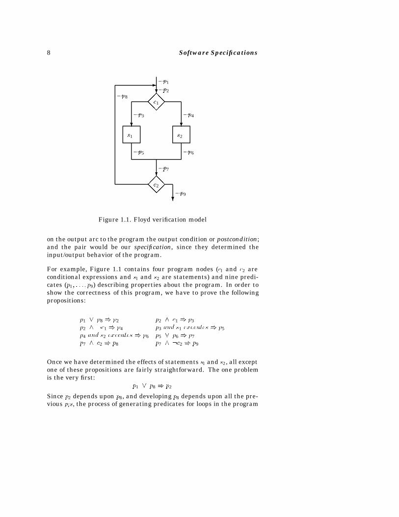
Figure 1.1. Floyd verification model
on the output arc to the program the output condition or postcondition;and the pair would be our specification, since they determined theinput/output behavior of the program.
For example, Figure 1.1 contains four program nodes (c1 and c2 areconditional expressions and s1 and s2 are statements) and nine predi-cates (p1� � � � � p9) describing properties about the program. In order toshow the correctness of this program, we have to prove the followingpropositions:
p1 � p8 p2 p2 c1 p3p2 �c1 p4 p3 and s1 executes p5p4 and s2 executes p6 p5 � p6 p7p7 c2 p8 p7 �c2 p9
Once we have determined the effects of statements s1 and s2, all exceptone of these propositions are fairly straightforward. The one problemis the very first:
p1 � p8 p2
Since p2 depends upon p8, and developing p8 depends upon all the pre-vious pis, the process of generating predicates for loops in the program
Introduction 9
becomes very difficult. It would take a further development by Hoareto fix this problem.
In 1969, Hoare [29] introduced the axiomatic model for program ver-ification which put Floyd’s model into the formal context of predicatelogic. His basic approach was to extend our formal mathematical the-ory of predicate logic with programming language concepts. His basicnotation was: fPgSfQg, meaning that if P were the precondition beforethe execution of a statement S, and if S were executed, then postcondi-tion Q would be true. Since a program is a sequence of statements, wesimply needed a set of axioms to describe the behavior of each state-ment type and a mechanism for executing statements sequentially. Aswill be shown later, this model simplifies but does not eliminate theproblems with loop predicates as given in the Floyd model.
�� A BRIEF SURVEY OF TECHNIQUES
Since the late 1960s and the developments of Floyd and Hoare, sev-eral models for program verification have been developed. We brieflysummarize them here and will describe them in greater detail in laterchapters.
���� Axiomatic Veri�cation
This is the technique previously described by Floyd and Hoare. We cangive a series of axioms describing the behavior of each statement type,and prove, using formal mathematical logic, that the program has thedesired pre- and postconditions.
For example, given the two propositions: fPgS1fQg and fQgS2fRg, wecan infer that if we execute both statements, we get: fPgS1;S2fRg.Similarly, if we can prove the following proposition: R T , we canthen state: fPgS1;S2fTg. Continuing in this manner, we build up aproof for the entire program. We can extend this model to include datadeclarations, arrays, and procedure invocation.
Dijkstra [10] developed a model similar to Hoare’s axiomatic modelwhich he called predicate transforms, based upon two notions: (a) theweakest precondition of a statement; and (b) guarded commands andnondeterministic execution.
10 Software Specifications
� Weakest preconditionThe weakest precondition to a given statement S and postconditionQ isthe largest initial set of states for which S terminates and Q is true. Aweakest precondition is also called a predicate transformer since we areable, in many cases, to derive from a given postcondition the precon-dition that fulfills this definition. If P is the weakest precondition, wewrite P � wp�S�Q�. For example, in order to have a variable x equal to3 after the assignment statement “x :� x�1”, the program state prior tothis statement must have x equal to 2. Therefore, wp�x :� x� 1� x � 3�is the set of all program states such that x has value 2.
As observed in Gries [23], we can prove several theorems from thisbasic definition:
wp�S� false� � falseif P Q then wp�S� P � wp�S�Q�wp�S� P �Q� � wp�S� P ��wp�S�Q�wp�S� P Q� � wp�S� P �wp�S�Q�
� Guarded commandsDijkstra realized that many algorithms were easier to write nondeter-ministically, that is, “if this condition is true then do this result.” Aprogram is simply a collection of these operations, and whenever anyof these conditions apply, the operation occurs. This concept is also thebasis for Prolog execution.
The basic concept is the guard (��). The statement:
if a1 � b1 �� � � � �� an � bn �
means to execute any bi if the corresponding ai is true.
From these, we can build up a model very similar to the Hoare axioms,as we will later show in Chapter 4.
���� Algebraic Speci�cation
The use of modularization, datatypes, and object oriented programminghave led to a further model called algebraic specifications, as developedby Guttag. In this model we are more concerned about the behavior ofobjects defined by programs rather than the details of their implemen-tation. For example, “What defines a data structure called a stack?”Any such description invariably includes the example of taking traysoff and on a pile of such trays in a cafeteria and moving your hands up
Introduction 11
l l
� � � � � � � � � �
�
���o
��
�������
CBA
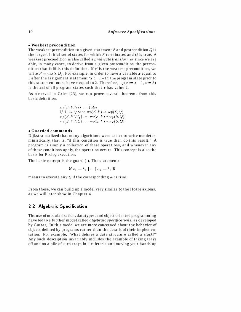
Figure 1.2. Memory model of storage
and down. More formally, we are saying that a push of a tray onto thestack is the inverse of the pop operation taking it off the stack. Or inother words, if S is a stack and x is an object, push and pop obey therelationship
pop�push�S� x�� � S
That is, if you add x to stack S and then pop it off, you get S back again.
By adding a few additional relationships, we can formally define howa stack must behave. We do not care how it is implemented as long asthe operations of push and pop obey these relationships. That is, theserelationships now form a specification for a stack.
���� Storage
Before discussing the remaining techniques, a slight digression con-cerning assignment and memory storage is in order. Consider thefollowing statement: C :� A� B. This statement contains two classesof components: (a) a set of data objects fA�B�Cg and (b) operatorsf�� :�g.
In most common languages like FORTRAN, Pascal, C, or Ada, opera-tors are fixed and changes are made to data. Storage is viewed as asequence of cells containing “memory objects.” The various operatorsaccess these memory objects, change them, (e.g., accessing A andB andadding them together) and placing the resulting object in the locationfor C (Figure 1.2). An ordered collection of colored marbles is probablythe mental image most people have of memory.
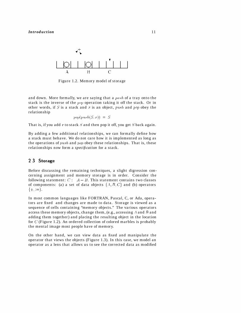
On the other hand, we can view data as fixed and manipulate theoperator that views the objects (Figure 1.3). In this case, we model anoperator as a lens that allows us to see the corrected data as modified
12 Software Specifications
����������
����������
����������
����������
����������
����������
����������
����������
����������
����������
CBA
Figure 1.3. Applicative model of storage
ll�
����������
������������
���
��������������������������������������������������������������������
��������������������������������������������������������������������
����������
����������
����������
����������
����������
����������
����������
����������
����������
CBA
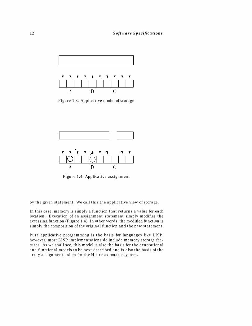
Figure 1.4. Applicative assignment
by the given statement. We call this the applicative view of storage.
In this case, memory is simply a function that returns a value for eachlocation. Execution of an assignment statement simply modifies theaccessing function (Figure 1.4). In other words, the modified function issimply the composition of the original function and the new statement.
Pure applicative programming is the basis for languages like LISP;however, most LISP implementations do include memory storage fea-tures. As we shall see, this model is also the basis for the denotationaland functional models to be next described and is also the basis of thearray assignment axiom for the Hoare axiomatic system.
Introduction 13
���� Functional Correctness
A program can be considered as a function from some input domainto some output domain. If we can also represent a specification as afunction, we simply have to show that they are equivalent functions.
Using the box notation of Mills [45], if p is a program, then p is definedto be the function that the program produces. If f is the specificationof this program, then verification means showing the equivalence off � p . While this in general is an undecidable property, we candevelop conditions of certain programs where we can show this, thatis, are there cases where we can compare the expected behavior of theprogram with the actual behavior?
In particular, if a program p is a sequence of statements s1� � � � � sn,then p is just the functional composition of each individual statementfunction s1 � � � sn .
We later give several axioms for deriving statement functions fromprogramming language statements and present techniques for provingthis equivalence.
���� Operational Semantics
The final model of verification we shall discuss is the operational model.In this case, model the program using some more abstract interpreter,show that the program and the abstracted program have equivalentproperties, and “execute” the program in the abstract model. Whatevereffects the abstracted program show will be reflected in the concreteprogram.
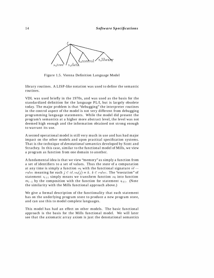
The first such model based upon this technique was the Vienna Defini-tion Language (VDL).2 This model extended the parse tree of a programinto a “tree interpreter.” (See Figure 1.5). While the parse tree (com-ponent s tree) was a static component of this model, some componentslike the program store (i.e., data storage component s data) and internalcontrol (s control) were dynamic and changed over time. Other compo-nents, like the library (i.e., “microprogrammed” semantic definition ofeach statement type in s library), were also static. The semantic defi-nition of the language was the set of interpreter routines built into the
2Not to be confused with the Vienna Development Method (VDM) to be described later.
14 Software Specifications
��
��
QQQQ
XXXXXXXXXX����
TTTT
JJJJ
SSS
���
���
�
s tree s datas control s library
Figure 1.5. Vienna Definition Language Model
library routines. A LISP-like notation was used to define the semanticroutines.
VDL was used briefly in the 1970s, and was used as the basis for thestandardized definition for the language PL/I, but is largely obsoletetoday. The major problem is that “debugging” the interpreter routinesin the control aspect of the model is not very different from debuggingprogramming language statements. While the model did present theprogram’s semantics at a higher more abstract level, the level was notdeemed high enough and the information obtained not strong enoughto warrant its use.
A second operational model is still very much in use and has had majorimpact on the other models and upon practical specification systems.That is the technique of denotational semantics developed by Scott andStrachey. In this case, similar to the functional model of Mills, we viewa program as function from one domain to another.
A fundamental idea is that we view “memory” as simply a function froma set of identifiers to a set of values. Thus the state of a computationat any time is simply a function mi with the functional signature id�value meaning for each j � id�mi�j� � k� k � value. The “execution” ofstatement si�1 simply means we transform function mi into functionmi�1 by the composition with the function for statement si�1. (Notethe similarity with the Mills functional approach above.)
We give a formal description of the functionality that each statementhas on the underlying program store to produce a new program store,and can use this to model complete languages.
This model has had an effect on other models. The basic functionalapproach is the basis for the Mills functional model. We will latersee that the axiomatic array axiom is just the denotational semantics
Introduction 15
assignment property.
�� SEMANTICS VERSUS SPECIFICATIONS
In the discussion so far, the terms “semantics,” “verification,” and “spec-ification” have been mostly intermixed with no clear distinction amongthem. They are highly interrelated, generally describe similar proper-ties, and their order above generally follows the historical developmentof the field.
Initially (duriing the late 1950s through mid-1960s), the problem was todescribe the semantics of a programming language, using techniqueslike attribute grammars and VDL-like operational semantics. Thethrust through the 1970s was the proving of the (functional) correctnessof a program, or program verification. Today, we are interested inbuilding valid systems, that is, programs that meet their specifications.
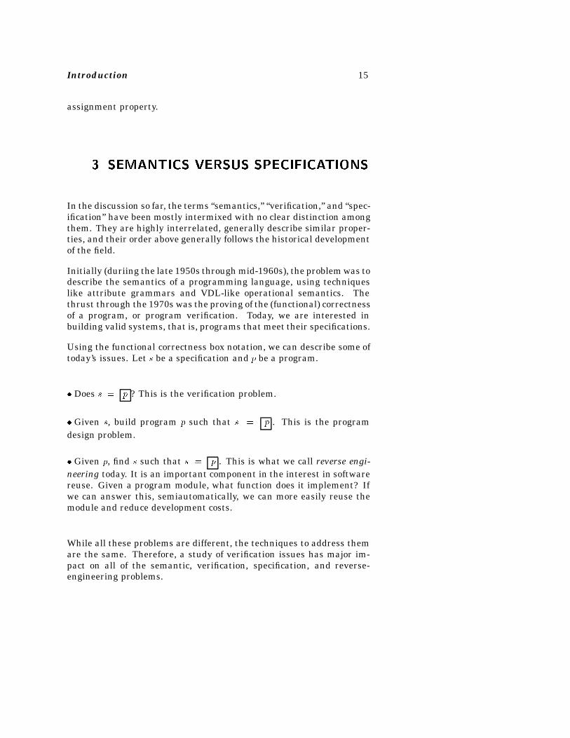
Using the functional correctness box notation, we can describe some oftoday’s issues. Let s be a specification and p be a program.
� Does s � p ? This is the verification problem.
� Given s, build program p such that s � p . This is the programdesign problem.
� Given p, find s such that s � p . This is what we call reverse engi-neering today. It is an important component in the interest in softwarereuse. Given a program module, what function does it implement? Ifwe can answer this, semiautomatically, we can more easily reuse themodule and reduce development costs.
While all these problems are different, the techniques to address themare the same. Therefore, a study of verification issues has major im-pact on all of the semantic, verification, specification, and reverse-engineering problems.
16 Software Specifications
�� LIMITATIONS OF FORMAL SYSTEMS
Although research on formal methods is a worldwide activity, culturaldifferences have emerged. Currently, the general view in the UnitedStates is that verification is a mechanism for proving the equivalencebetween a specification and a program. Since real programs imple-mented on real computers using real compilers have numerous limita-tions, the proofs are necessarily hard and verification has made littleimpact in industry.
On the other hand, the European view is that verification is a mecha-nism for showing the equivalence between a specification and a design.Since a software design is somewhat removed from the actual imple-mentation, verification is easier, although one still has the remainingproblem of showing that the design does agree with the implemen-tation. Because of this, verification is generally more prevalent inEuropean development activities than in the U.S.
Now that you are “sold” on the value of such formal models, we mustput these techniques in perspective. Hall [28] listed seven “myths” offormal systems. It is important to understand these concepts as partof learning about the techniques themselves.
1. Formal methods can guarantee that software is perfect. As we haveshown, all the formal techniques rely on abstracting a program intoan abstract specification that closely approximates reality. However,this formal specification is rarely exact, so the resulting program onlyapproximates what you specify. If done well, then this approximationis close enough. However, even simple propositions like “x � 1 � xfor integer x” fail with real machines with fixed word size and limitedrange of integer values.
In addition, we cannot forget that mathematical proofs may have er-rors in them. Formal proofs certainly help, but are no guarantee ofperfection.
2. They work by proving the programs are correct. As stated at thebeginning, we are interested in more than just functional correctness.Cost, development time, performance, security, and safety are all prop-erties that are part of a complete specification.
3. Only highly critical systems benefit from their use. It has been shownthat almost any large system will benefit from using formal techniques.
Introduction 17
The cleanroom is a technique to informally use functional correctnesson large software projects. It has been used at IBM, NASA GodddardSpace Flight Center and at the University of Maryland (albeit withsmall student projects in that case). In all instances, reliability washigher, and development effort was sometimes dramatically lower.
4. They involve complex mathematics. These techniques involve preci-sion, not complex mathematics. There is nothing in this book that awell-informed college undergraduate should not be able to understand.Precision takes much of the ambiguity out of a 300-page informal En-glish specification that is more typical in industry today.
5. They increase the cost of development. They do increase the costof program design, since one must develop the abstract model of thespecification more explicitly that is usually done. For managers im-patient with programmers not writing any “code,” this certainly lookslike an increase in costs. But as numerous studies have shown (e.g.,the cleanroom studies above), the project’s overall costs are lower sincethe time-consuming and expensive testing phases are dramatically re-duced.
6. They are incomprehensible to clients. It is our belief that a 300page English text of ambiguous statements is more incomprehensible.In addition, the role of formal methods is to help the technical staffunderstand what they are to build. One must still translate this into adescription for the eventual user of the system.
7. Nobody uses them for real projects. This is simply not true. Severalcompanies depend upon formal methods. Also, various modificationsto some of these techniques are used in scattered projects throughoutindustry. It is unfortunately true, however, that few projects use suchtechniques, which results in most of the problems everyone is writingabout.
The following section will give the notation we will use throughout thisbook, and the following chapters will present these techniques outlinedhere in more detail.
�� PROPOSITIONAL CALCULUS
Much of the theory of program verification is built upon mathemat-ical logic. This section is a brief review of some of these concepts.
18 Software Specifications
The propositional calculus is a simple language for making statements(propositions) that may be viewed as true or false. Strings in this lan-guage are called formulae.
The syntax for the propositional calculus is
� set of symbols
variables:A, B, P, Q, R, � � �
constants:T, F
connectives:, �, �,
parentheses:(, )
� rules for forming legal strings of these symbols, e.g. a formula isdefined as
a variable
a constant
a string: if A and B are formulae, so are AB, A�B, �A and A B
We must now define the semantics of propositional calculus. An inter-pretation is a way of understanding a formula, encoding some informa-tion. Truth values are assigned to formulae as follows:
� T has value true
� F has value false
� Variables can take on either true or false
� (A B) is true if A is true and B is true, is false otherwise
� (A�B) is true if A is true or B is true, is false otherwise
� �A is true if A if false, is false if A is true
� (AB) is true if A is false or B is true
Definitions:
truth assignment: A truth assignment is a mapping of the variableswithin a formula into the value true or false.
Introduction 19
satisfiable: A formula is satisfiable if there exists some truth assign-ment under which the formula has truth value true.
valid: A formula is a tautology, or valid, if it has truth value true underall possible truth assignments.
unsatisfiable: A formula is unsatisfiable if it has the truth value falsefor all possible truth assignments.
decidable: Propositional logic is decidable: there exists a procedure todetermine, for any formula, if it is satisfiable (and hence valid) or not,e.g., truth tables.
���� Truth Tables
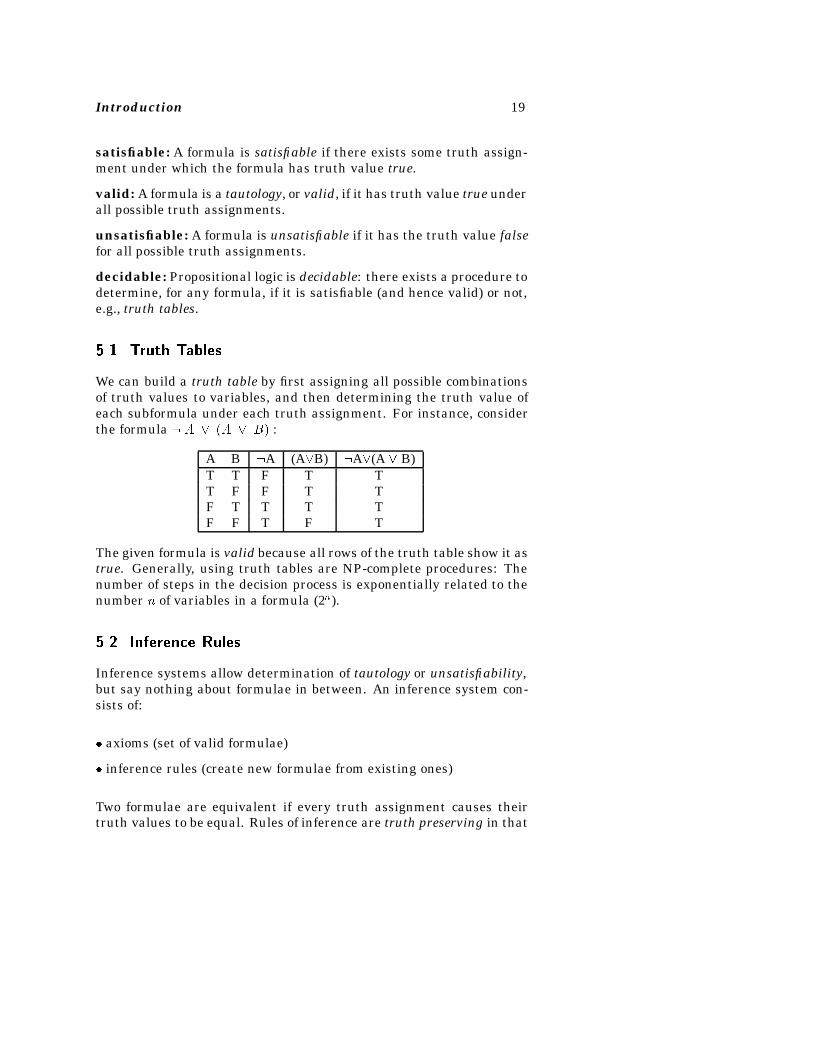
We can build a truth table by first assigning all possible combinationsof truth values to variables, and then determining the truth value ofeach subformula under each truth assignment. For instance, considerthe formula � A � �A � B� :
A B �A (A�B) �A�(A � B)T T F T TT F F T TF T T T TF F T F T
The given formula is valid because all rows of the truth table show it astrue. Generally, using truth tables are NP-complete procedures: Thenumber of steps in the decision process is exponentially related to thenumber n of variables in a formula (2n).
���� Inference Rules
Inference systems allow determination of tautology or unsatisfiability,but say nothing about formulae in between. An inference system con-sists of:
� axioms (set of valid formulae)
� inference rules (create new formulae from existing ones)
Two formulae are equivalent if every truth assignment causes theirtruth values to be equal. Rules of inference are truth preserving in that
20 Software Specifications
they transform a formula (conjunction of members of a set of formulae)into an equivalent formula. Starting with axioms (which are valid),then each subsequent formula derived with inference rules is also valid.This is soundness: If only valid formulae can be derived, the inferencesystem is sound.
We say an inference system is complete if it can derive all formulaewhich are valid. For example:
� Axioms
1. P (Q P)
2. (S (P Q)) ((S P) (S Q))
3. � (� P) P
� Inference rules
1. From (A B) and A, conclude B (modus ponens)
2. From A, may get A’ by substituting a variable y for variable xthroughout A.
This system is sound and complete.
Axioms are proven valid with truth tables. Another formula may thenbe proven valid by discovering (manufacturing) a sequence of rules toapply to the axioms to get the formula.
In some cases, we want a result if some previous assumption is true.For example, if p is assumed true, then can we infer q? In such asituation we will use the notation p � q. In fact to be quite formal,given our inference system, any result q that we can infer from ouraxioms is properly written as true � q, or more simply � q.
In most situations, p � q and p q behave quite similarly, and we willavoid this added level of complexity in this book. But they are quitedifferent. is a binary operator applied to predicates, while � is aninference rule. For the most part we can ignore the difference, however,even in our treatment here, we need to differentiate between the twoconcepts. For example, we will see that the recursive procedure callrule in Chapter 2 and VDM in Chapter 7 both need to refer to �.
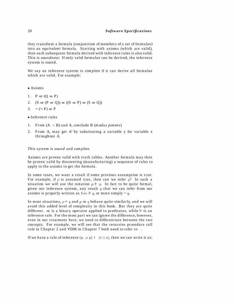
If we have a rule of inference �p q� � �r s�, then we can write it as:
Introduction 21
p q
r s
We will interpret this to mean that if we can show the formula abovethe ‘bar’ (p q) to be valid (either as an assumption or as a previouslyderived formula), then we can derive the formula below the ‘bar’ (r s)as valid. We shall use this notation repeatedly to give our inferencerules in this book.
If the relationship works both ways (i.e., p q and q p), then we willuse the notation:
p
q
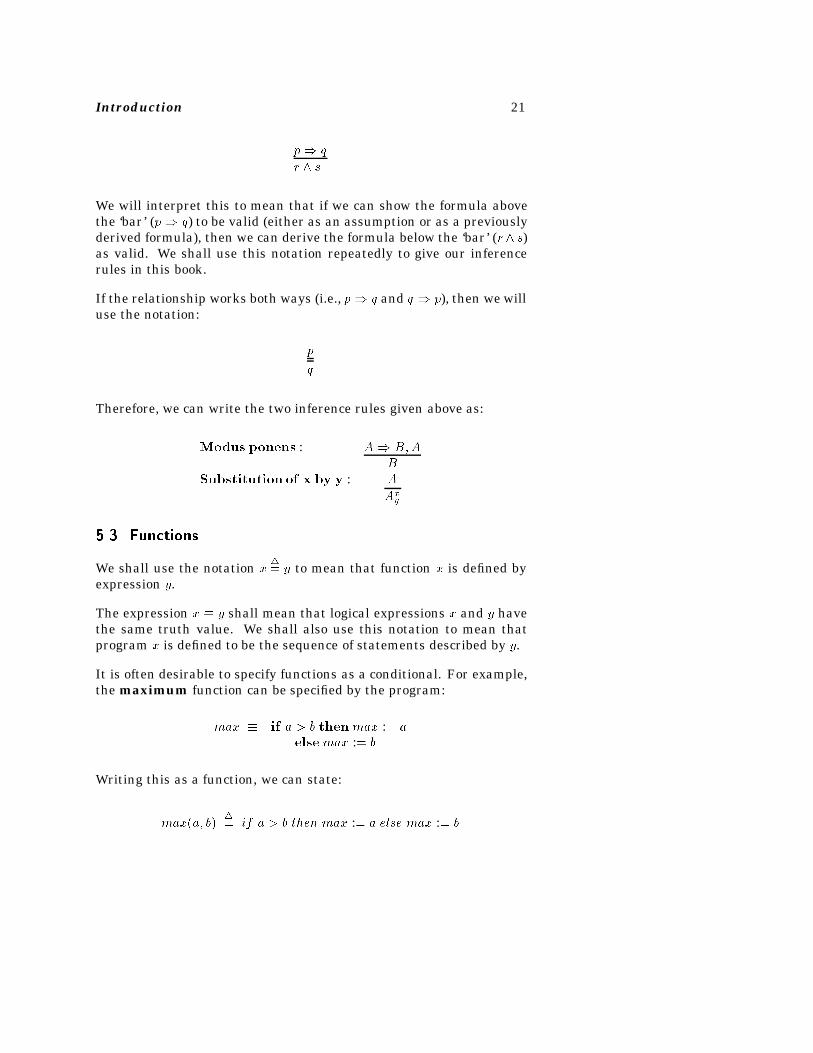
Therefore, we can write the two inference rules given above as:
Modus ponens : A B�AB
Substitution of x by y : A
Axy
���� Functions
We shall use the notation x�� y to mean that function x is defined by
expression y.
The expression x � y shall mean that logical expressions x and y havethe same truth value. We shall also use this notation to mean thatprogram x is defined to be the sequence of statements described by y.
It is often desirable to specify functions as a conditional. For example,the maximum function can be specified by the program:
max � if a � b thenmax :� aelsemax :� b
Writing this as a function, we can state:
max�a� b��� if a � b then max :� a else max :� b
22 Software Specifications
and can then write max�a� b� or max�x� y�.
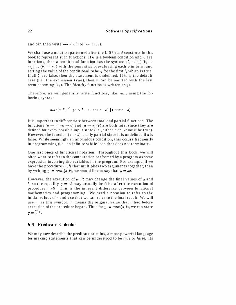
We shall use a notation patterned after the LISP cond construct in thisbook to represent such functions. If bi is a boolean condition and ci arefunctions, then a conditional function has the syntax: �b1 � c1�j�b2 �c2�j � � � j�bn � cn� with the semantics of evaluating each bi in turn, andsetting the value of the conditional to be ci for the first bi which is true.If all bi are false, then the statement is undefined. If bn is the defaultcase (i.e., the expression true), then it can be omitted with the lastterm becoming �cn�. The Identity function is written as ��.
Therefore, we will generally write functions, like max, using the fol-lowing syntax:
max�a� b��� �a � b � max :� a� j �max :� b�
It is important to differentiate between total and partial functions. Thefunctions �a � b�j�a� c� and �a � b�j�c� are both total since they aredefined for every possible input state (i.e., either a or �a must be true).However, the function �a� b� is only partial since it is undefined if a isfalse. While seemingly an anomalous condition, this occurs frequentlyin programming (i.e., an infinite while loop that does not terminate.
One last piece of functional notation. Throughout this book, we willoften want to refer to the computation performed by a program as someexpression involving the variables in the program. For example, if wehave the procedure mult that multiplies two arguments together, thenby writing y :� mult�a� b�, we would like to say that y � ab.
However, the execution of mult may change the final values of a andb, so the equality y � ab may actually be false after the execution ofprocedure mult. This is the inherent difference between functionalmathematics and programming. We need a notation to refer to theinitial values of a and b so that we can refer to the final result. We willuse � as this symbol.
�a means the original value that a had before
execution of the procedure began. Thus for y :� mult�a� b�, we can statey �
�a�
b .
���� Predicate Calculus
We may now describe the predicate calculus, a more powerful languagefor making statements that can be understood to be true or false. Its
Introduction 23
syntax is:
� predicate symbols �P�Q�R� ���������� ����
� variables �x� y� z� ����
� function names �f� g� h� ����
� constants (0-argument functions) �a� b� c� ����
� quantifiers ( �, � )
� logical connectives ( , �, �, )
� logical constants �T� F �
An atomic formula is either:
� a logical constant (T or F )
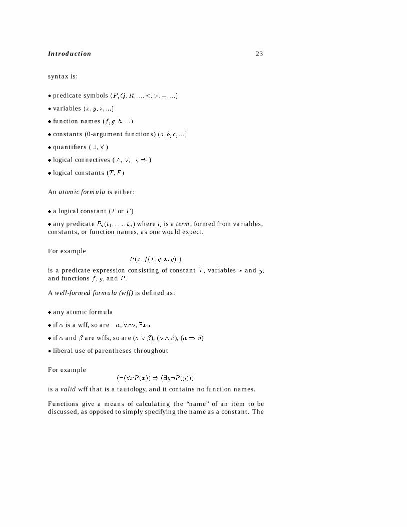
� any predicate Pn�t1� � � � � tn� where ti is a term, formed from variables,constants, or function names, as one would expect.
For exampleP �x� f�T� g�x� y���
is a predicate expression consisting of constant T , variables x and y,and functions f , g, and P .
A well-formed formula (wff) is defined as:
� any atomic formula
� if � is a wff, so are ��, �x�, �x�
� if � and � are wffs, so are (� � �), (� �), (� �)
� liberal use of parentheses throughout
For example����xP �x�� ��y�P �y���
is a valid wff that is a tautology, and it contains no function names.
Functions give a means of calculating the “name” of an item to bediscussed, as opposed to simply specifying the name as a constant. The
24 Software Specifications
added power is akin to using arrays with variables as subscripts, asopposed to using only constants as subscripts.
We say a variable in a wff is bound if it is in the scope of some quantifier(shown by parentheses unless obvious). A variable is free if it is notbound. For example: in �x�y�Q�x� f�y� z��� x and y are bound, and z isfree.
In predicate calculus, an interpretation I is analogous to truth assign-ment in propositional calculus.
� set of elements D (the domain)
� each n-place function name fn is assigned a total function hfni: Dn �D
� each constant, each free variable is mapped intoD (i.e., given a value)
� each n-place predicate name Pn is assigned a total functionhPni: Dn � f T , F g.
If W is a wff, and I is an interpretation, then �W� I� denotes the truthvalue of the statement that the two together represent.
1. W is valid iff (W,I) is true for every I.
2. W is satisfiable iff (W,I) is true for some I.
3. W is unsatisfiable iff (W,I) is true for no I (is false for all I).
However, the predicate calculus is not decidable. There exist W suchthat it cannot be determined whether there is an interpretation I suchthat �W� I� is valid. There are complete and sound inference systemsfor all three of the following:
1. valid: can prove wff W by deriving W from the axioms.
2. unsatisfiable: can prove wff W by deriving the negation of W fromthe axioms (assuming � (A � A) is an axiom of the system).
3. satisfiable: W is satisfiable if can say nothing about W , since neitherderivation (A and � A) will terminate.
Introduction 25
���� Quanti�ers
The propositional calculus is a zero-order language containing onlyconstants without functions. The predicate calculus is a first-orderlanguage containing functions that compute values. There exist higher-order languages (second, third, etc.), having functions that compute(functions that compute � � � (functions that compute values) � � � ).
Example:
�x�y�x � y � x � y�
This is common notation, though the relation could be written moreaccurately as ��� �x� y��� �x� y��.
However, is that statement True or false (i.e., a tautology)? That de-pends on the interpretation:
� If we let D be the set of natural numbers, with normal arithmetic thethis wff is true.
� If let D be the set of all integers, then this wff is false.
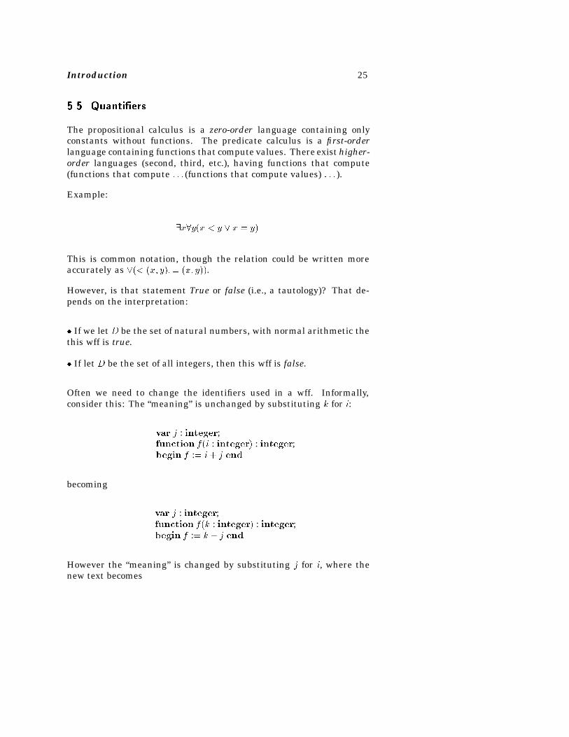
Often we need to change the identifiers used in a wff. Informally,consider this: The “meaning” is unchanged by substituting k for i:
var j : integer;function f�i : integer� : integer;begin f :� i� j end
becoming
var j : integer;function f�k : integer� : integer;begin f :� k � j end
However the “meaning” is changed by substituting j for i, where thenew text becomes
26 Software Specifications
var j : integer;function f�j : integer� : integer;begin f :� j � j end
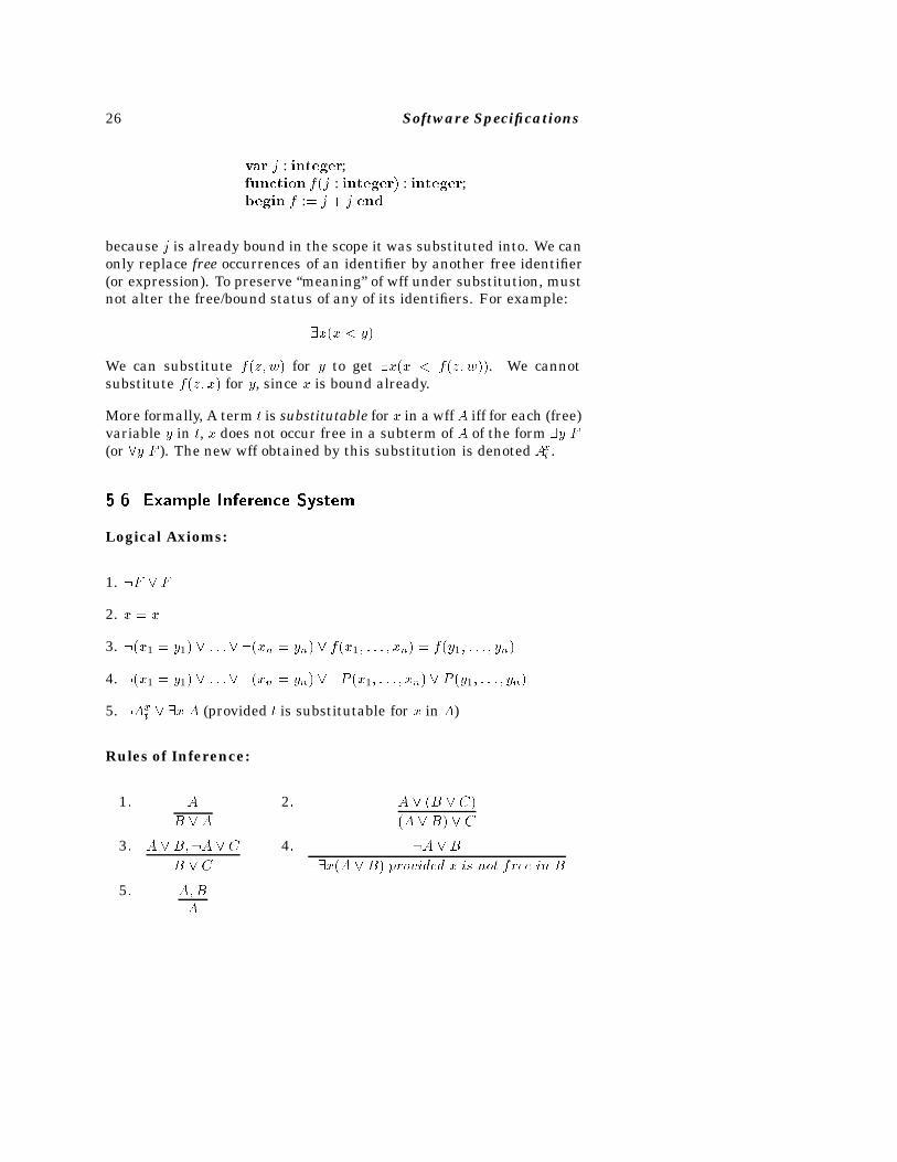
because j is already bound in the scope it was substituted into. We canonly replace free occurrences of an identifier by another free identifier(or expression). To preserve “meaning” of wff under substitution, mustnot alter the free/bound status of any of its identifiers. For example:
�x�x � y�
We can substitute f�z� w� for y to get �x�x � f�z� w��. We cannotsubstitute f�z� x� for y, since x is bound already.
More formally, A term t is substitutable for x in a wffA iff for each (free)variable y in t, x does not occur free in a subterm of A of the form �y F(or �y F ). The new wff obtained by this substitution is denoted Axt .
���� Example Inference System
Logical Axioms:
1. �F � F
2. x � x
3. ��x1 � y1� � � � �� ��xn � yn� � f�x1� � � � � xn� � f�y1� � � � � yn�
4. ��x1 � y1� � � � �� ��xn � yn� � �P �x1� � � � � xn� � P �y1� � � � � yn�
5. �Axt � �x A (provided t is substitutable for x in A)
Rules of Inference:
1� A 2� A � �B �C�
B �A �A �B� � C
3� A �B��A �C 4� �A �B
B � C ��x�A �B� provided x is not free in B
5� A�BA
Introduction 27
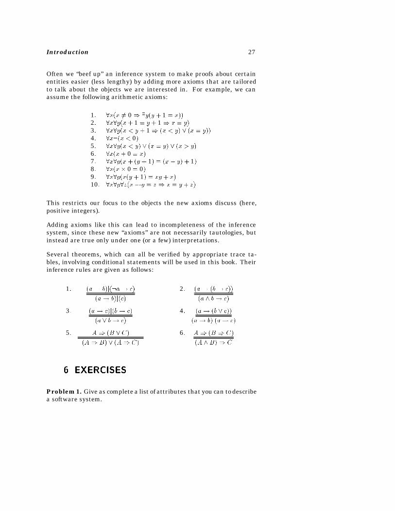
Often we “beef up” an inference system to make proofs about certainentities easier (less lengthy) by adding more axioms that are tailoredto talk about the objects we are interested in. For example, we canassume the following arithmetic axioms:
1� �x�x �� 0 �y�y � 1 � x��2� �x�y�x � 1 � y � 1 x � y�3� �x�y�x � y � 1 �x � y� � �x � y��4� �x��x � 0�5� �x�y�x � y� � �x � y� � �x � y�6� �x�x� 0 � x�7� �x�y�x � �y � 1� � �x� y� � 1�8� �x�x� 0 � 0�9� �x�y�x�y � 1� � xy � x�10� �x�y�z�x � y � z x � y � z�
This restricts our focus to the objects the new axioms discuss (here,positive integers).
Adding axioms like this can lead to incompleteness of the inferencesystem, since these new “axioms” are not necessarily tautologies, butinstead are true only under one (or a few) interpretations.
Several theorems, which can all be verified by appropriate trace ta-bles, involving conditional statements will be used in this book. Theirinference rules are given as follows:
1� �a� b�j��a� c� 2� �a� �b� c��
�a� b�j�c� �a b� c�
3� �a� c�j�b� c� 4� �a� �b � c��
�a � b� c� �a� b�j�a� c�
5� A �B �C� 6� A �B C�
�A B� � �A C� �A B� C
�� EXERCISES
Problem 1. Give as complete a list of attributes that you can to describea software system.
28 Software Specifications
Problem 2. Define the binary operator � as:
A� B�� �A B� �B A�
Show that DeMorgan’s laws are valid:
�A B� � ���A � �B��A �B� � ���A �B�
�� SUGGESTED READINGS
Jon Bentley’s collection of writings
� J. Bentley, Programming Pearls, Addison-Wesley, Reading, MA, 1986.
is an excellent source of ideas for refining practical programming andproblem-solving skills. Chapter Four in particular, “Writing CorrectPrograms,” gives a nice introduction to the types of proof methodswhich will be discussed in this book. Likewise the book,
� D. Gries, The Science of Programming, Springer-Verlag, New York,1981.
is a magnificent textbook describing the process of program specifica-tion and development using predicate transforms.
Background material for this book consists of the following:
Understanding of context free languages, parsing, and general lan-guage structure. Compiler books like the following are helpful:
� A. Aho, R. Sethi, and J. Ullman, Compilers: Principles, Techniquesand Tools, Addison-Wesley, Reading, MA, 1986.
� C. N. Fischer and R. J. LeBlanc, Crafting a compiler, Benjamin Cum-mings, Menlo Park, CA, 1988.
Understanding the structure of programming languages and their ex-ecution model in typical von Neumann architectures:
Introduction 29
� T. W. Pratt, Programming Languages: Design and Implementation,Second Edition, Prentice-Hall, Englewood Cliffs, NJ, 1984.
� R. Sethi, Programming Languages: Concepts and Constructs, Addi-son-Wesley, Reading MA, 1989.
Some references for specification systems include:
� A. Hall, “Seven Myths of Formal Methods,” IEEE Software, Vol. 7,No. 5, September 1990, pp. 11-19.
� J. Wing, “A Specifier’s Introduction to Formal Methods,” IEEE Com-puter, Vol. 23, No. 9, September 1990, pp. 8-24.
� J. Woodcock and M. Loomes, Software Engineering Mathematics,Addison-Wesley, Reading, MA, 1988. (This is a theory using a Z-likenotation.)
� D. Craigen (Ed.), Formal methods for trustworthy computer systems,Springer-Verlag, New York, 1990.

30 Software Specifications
Chapter 2
The Axiomatic Approach
An axiomatic approach requires both axioms and rules of inference. Forour purposes, we will accept the axioms of arithmetic which character-ize the integers and the usual rules of logical inference as discussedearlier (Chapter 1, Section 5). However, we do not seek to model justthe ‘world of integers’ but also the ‘world of computation,’ and hencewe need additional axioms and inference rules corresponding to theconstructs we intend to use as our programming language.
�� PROGRAMMING LANGUAGE AXIOMS
In order to build programs into our inference system, we must be ableto model a computation as a logical predicate. We adopt the notationfPgSfQg, where P and Q are assertions about the state of the compu-tation and S is a statement. This expression is interpreted as “If P ,called the precondition, is true before executing S and S terminatesnormally, then Q, called the postcondition, will be true.” This willallow us to model a simple “Algol-like” programming language. We dothis by adding the inference rules of composition and consequence:
Composition :fPgS1fQg� fQgS2fRg
fPgS1;S2fRg
31
32 Software Specifications
Consequence1 :fPgSfRg� R Q
fPgSfQg
Consequence2 :P R� fRgSfQg
fPgSfQg
If we are to have confidence in a program which has been proven tobe partially correct by this axiomatic method, then it is important forus to believe in the axioms and inference rules accepted up front. Agood way to find motivation for the choice of these inference rules is toexamine the Floyd-style flow chart associated with each drawing.
The rule of composition is the basic mechanism which allows us to“glue” together two computations (i.e., two statements). If the postcon-dition of one statement is the same as the precondition of the followingstatement, then the execution of both of them proceeds as expected.
The rules of consequence build in our predicate logic rules of inference.We can use these to permit us to use alternative pre- and postconditionsto any statement as long as we can derive them via our mathematicalsystem.
Given this logical model, we need to build in the semantics of a givenprogramming language. We will use the following BNF to describe asimple Algol-like language:
� stmt �::� � stmt �;� stmt �jif � expr � then � stmt �jif � expr � then � stmt � else � stmt �jwhile � expr � do � stmt �j � id � :� � expr �
where � id � and � expr � have their usual meanings. Note: Theexamples will be kept simple, and we will not worry about potentialambiguities such as programs like: � stmt �; if � expr � then �stmt �;� stmt �. that is, is this a “statement and an if” or “statement,if, and statement?” The examples will be clear as to meaning.
The basic approach is a “backwards verification” method. For example,for the assignment, we will define the axiom so that given the resultof an assignment statement, what must have been true prior to theexecution of the statement in order for the result to occur? Or in otherwords, given the postcondition to an assignment statement, what is itsprecondition?
The Axiomatic Approach 33
We accept the assignment axiom schema
fP xy gx :� yfPg
Here P xy represents the expression P where all free occurrences of x
have been replaced by y. For example,
fz � x� y � 3gx :� x� y � 1fz � x� 4g
represents the effect of replacement of x by x� y � 1.
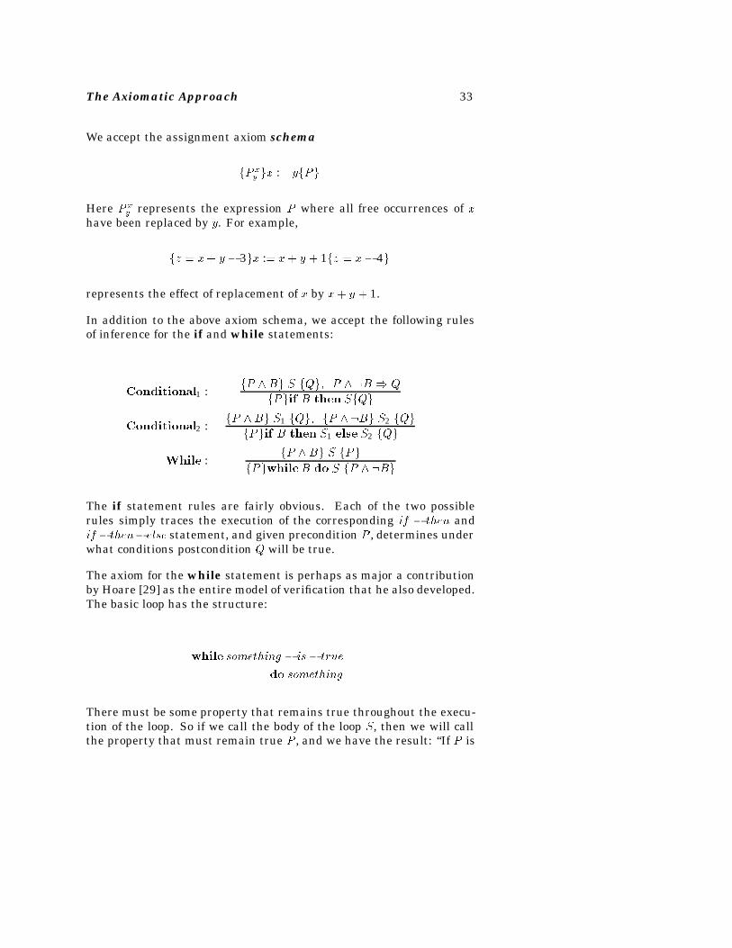
In addition to the above axiom schema, we accept the following rulesof inference for the if and while statements:
Conditional1 :fP Bg S fQg� P �B Q
fPgif B then SfQg
Conditional2 :fP Bg S1 fQg� fP �Bg S2 fQg
fPgif B then S1 else S2 fQg
While :fP Bg S fPg
fPgwhileB do S fP �Bg
The if statement rules are fairly obvious. Each of the two possiblerules simply traces the execution of the corresponding if � then andif � then� else statement, and given precondition P , determines underwhat conditions postcondition Q will be true.
The axiom for the while statement is perhaps as major a contributionby Hoare [29] as the entire model of verification that he also developed.The basic loop has the structure:
while something � is � true
do something
There must be some property that remains true throughout the execu-tion of the loop. So if we call the body of the loop S, then we will callthe property that must remain true P , and we have the result: “If P is
34 Software Specifications
true and we execute the loop, then P will remain true.” The condition‘and we execute the loop’ is just the predicate on the while statementB. This leads to the condition that: fP BgSfPg as the antecedentproperty on the while axiom. So if this antecedent is true, then afterthe loop ‘terminates,’ we still will have P true, and since the loop ter-minated, B must now be false, hence the axiom as given. Note we havenot proven that the loop does terminate. That must be shown and isoutside of this axiom system (see Section 1.2).
The property that remains true within the loop is called the invariantand it is at the heart of developing axiomatic proofs for programs. Whilethere is no algorithmic method for developing invariants, we later givesome ideas on how to proceed.
���� Example� Integer Division
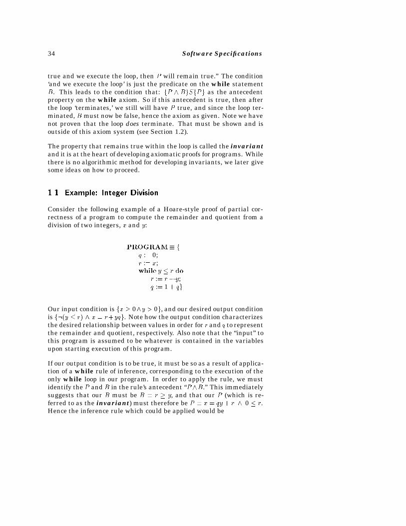
Consider the following example of a Hoare-style proof of partial cor-rectness of a program to compute the remainder and quotient from adivision of two integers, x and y:
PROGRAM � fq :� 0;r :� x;while y � r do
r :� r � y;q :� 1 � qg
Our input condition is fx � 0y � 0g, and our desired output conditionis f��y � r� x � r�yqg. Note how the output condition characterizesthe desired relationship between values in order for r and q to representthe remainder and quotient, respectively. Also note that the “input” tothis program is assumed to be whatever is contained in the variablesupon starting execution of this program.
If our output condition is to be true, it must be so as a result of applica-tion of a while rule of inference, corresponding to the execution of theonly while loop in our program. In order to apply the rule, we mustidentify the P and B in the rule’s antecedent “P B.” This immediatelysuggests that our B must be B � r � y, and that our P (which is re-ferred to as the invariant) must therefore be P � x � qy � r 0 � r.Hence the inference rule which could be applied would be
The Axiomatic Approach 35
fP r � ygr :� r � y; q :� q � 1fPgfPg while r � y do r :� r � y; q :� q � 1f P �Bg
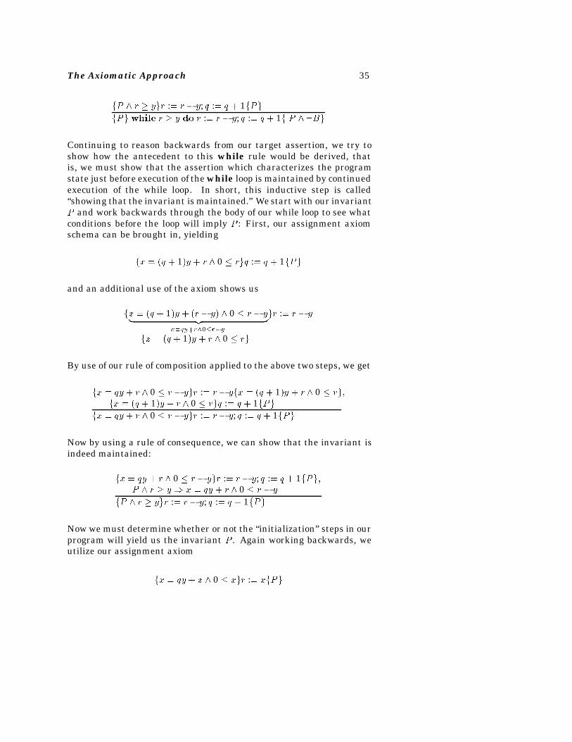
Continuing to reason backwards from our target assertion, we try toshow how the antecedent to this while rule would be derived, thatis, we must show that the assertion which characterizes the programstate just before execution of the while loop is maintained by continuedexecution of the while loop. In short, this inductive step is called“showing that the invariant is maintained.” We start with our invariantP and work backwards through the body of our while loop to see whatconditions before the loop will imply P : First, our assignment axiomschema can be brought in, yielding
fx � �q � 1�y � r 0 � rgq :� q � 1fPg
and an additional use of the axiom shows us
fx � �q � 1�y � �r � y� 0 � r � y� �z �x�qy�r�0�r�y
gr :� r � y
fx � �q � 1�y � r 0 � rg
By use of our rule of composition applied to the above two steps, we get
fx � qy � r 0 � r � ygr :� r � yfx � �q � 1�y � r 0 � rg�fx � �q � 1�y � r 0 � rgq :� q � 1fPg
fx � qy � r 0 � r � ygr :� r � y; q :� q � 1fPg
Now by using a rule of consequence, we can show that the invariant isindeed maintained:
fx � qy � r 0 � r � ygr :� r � y; q :� q � 1fPg�P r � y x � qy � r 0 � r � y
fP r � ygr :� r � y; q :� q � 1fPg
Now we must determine whether or not the “initialization” steps in ourprogram will yield us the invariant P . Again working backwards, weutilize our assignment axiom
fx � qy � x 0 � xgr :� xfPg
36 Software Specifications
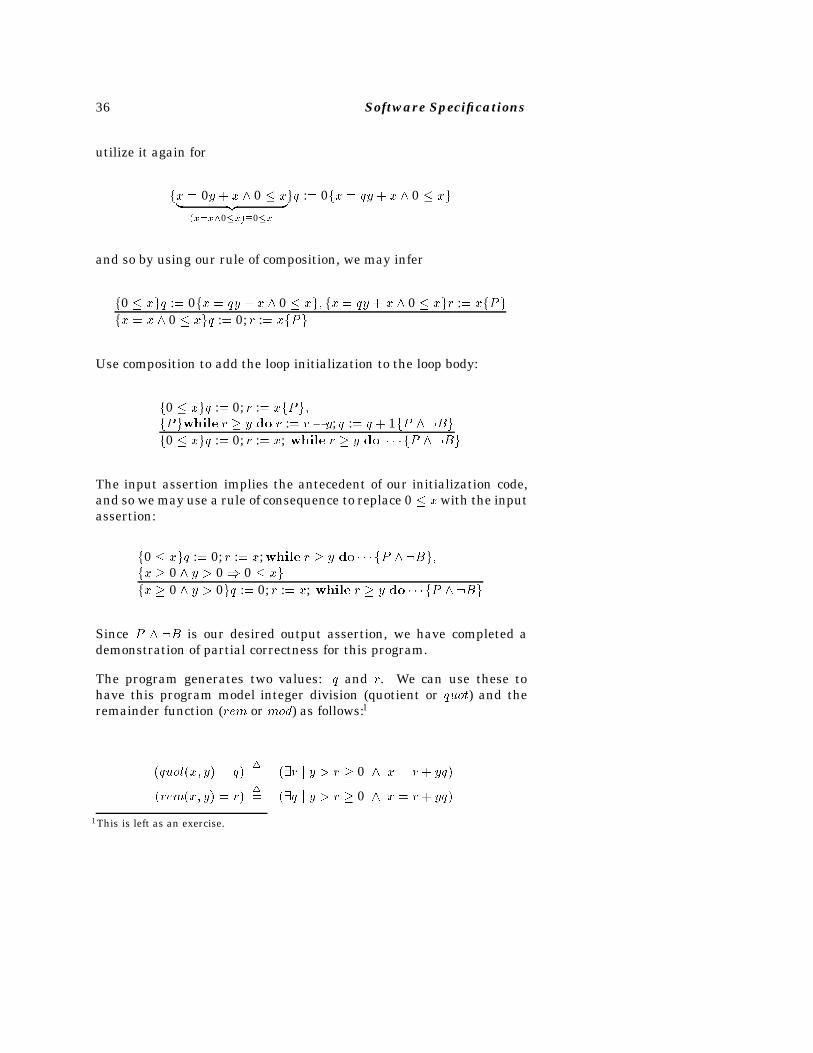
utilize it again for
fx � 0y � x 0 � x� �z ��x�x�0�x��0�x
gq :� 0fx � qy � x 0 � xg
and so by using our rule of composition, we may infer
f0 � xgq :� 0fx � qy � x 0 � xg� fx � qy � x 0 � xgr :� xfPgfx � x 0 � xgq :� 0; r :� xfPg
Use composition to add the loop initialization to the loop body:
f0 � xgq :� 0; r :� xfPg�fPgwhile r � y do r :� r � y; q :� q � 1fP �Bgf0 � xgq :� 0; r :� x; while r � y do � � � fP �Bg
The input assertion implies the antecedent of our initialization code,and so we may use a rule of consequence to replace 0 � xwith the inputassertion:
f0 � xgq :� 0; r :� x;while r � y do � � � fP �Bg�fx � 0 y � 0 0 � xg
fx � 0 y � 0gq :� 0; r :� x; while r � y do � � � fP �Bg
Since P �B is our desired output assertion, we have completed ademonstration of partial correctness for this program.
The program generates two values: q and r. We can use these tohave this program model integer division (quotient or quot) and theremainder function (rem or mod) as follows:1
�quot�x� y� � q��� ��r j y � r � 0 x � r � yq�
�rem�x� y� � r��� ��q j y � r � 0 x � r � yq�
1This is left as an exercise.
The Axiomatic Approach 37
We will use these results later.
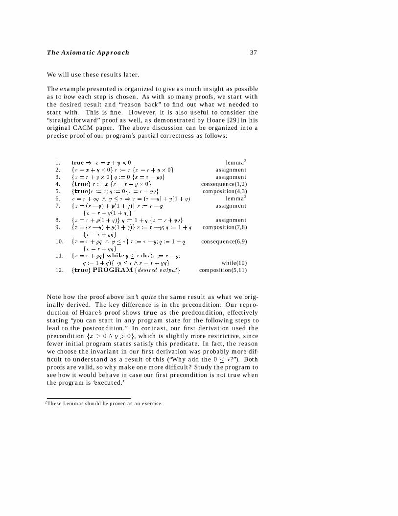
The example presented is organized to give as much insight as possibleas to how each step is chosen. As with so many proofs, we start withthe desired result and “reason back” to find out what we needed tostart with. This is fine. However, it is also useful to consider the“straightforward” proof as well, as demonstrated by Hoare [29] in hisoriginal CACM paper. The above discussion can be organized into aprecise proof of our program’s partial correctness as follows:
1. true � x � x� y � 0 lemma2
2. fx � x� y � 0g r :� x fx � r � y� 0g assignment3. fx � r � y � 0g q :� 0 fx � r � yqg assignment4. ftrueg r :� x fx � r � y� 0g consequence(1,2)5. ftruegr :� x; q :� 0fx � r � yqg composition(4,3)6. x � r � yq � y � r � x � �r� y� � y�1� q� lemma2
7. fx � �r � y� � y�1 � q�g r :� r � y assignmentfx � r � y�1 � q�g
8. fx � r � y�1 � q�g q :� 1� q fx � r � yqg assignment9. fx � �r � y� � y�1 � q�g r :� r � y; q :� 1 � q composition(7,8)
fx � r � yqg10. fx � r � yq � y � rg r :� r � y; q :� 1� q consequence(6,9)
fx � r � yqg11. fx � r � yqg while y � r do �r :� r � y;
q :� 1� q�f�y � r � x � r � yqg while(10)12. ftrueg PROGRAM fdesired outputg composition(5,11)
Note how the proof above isn’t quite the same result as what we orig-inally derived. The key difference is in the precondition: Our repro-duction of Hoare’s proof shows true as the predcondition, effectivelystating “you can start in any program state for the following steps tolead to the postcondition.” In contrast, our first derivation used theprecondition fx � 0 y � 0g, which is slightly more restrictive, sincefewer initial program states satisfy this predicate. In fact, the reasonwe choose the invariant in our first derivation was probably more dif-ficult to understand as a result of this (“Why add the 0 � r?”). Bothproofs are valid, so why make one more difficult? Study the program tosee how it would behave in case our first precondition is not true whenthe program is ‘executed.’
2These Lemmas should be proven as an exercise.
38 Software Specifications
���� Program Termination
We have shown the “partial correctness” of this introductory example,that is, if the program begins execution in a state satisfying the precon-dition, and if the program terminates, then the postcondition will betrue. But how do we know the program actually terminates? We canoften show termination by showing that the following two propertieshold:
1. Show that there is some property P which is positive within a loop.
2. Show that for each iteration of the loop, P is decremented by a fixedamount. That is Pi � Pi�1.
If both properties are true, and if the second property causes P todecrement (yet still be positive), then the only way this can be consistentis for the loop to terminate, or else the first property must become falseat some point.
Applying this principle to the previous example: The only variablesaffecting the loop test are y and r. The former does not change throughexecution, therefore we concentrate our investigation on what happensto the latter, r. Its initial value is x, which we know from the initial-ization of the program. In the case that y is strictly greater than xon input, then termination is certain, since the body of the while loopwould never be executed. Otherwise, r starts out greater than or equalto y and the loop begins execution. In the body of the loop, r is decre-mented by a positive value (we know it is positive by the precondition);in fact, this decrement is unavoidable. Hence, we may infer that in afinite number of iterations of the loop, r will be decremented to whereit is no longer the case that y � r and therefore the loop will exit. Allexecution paths have been accounted for, and hence we conclude thatthe program will indeed terminate when started in a state satisfyingthe precondition.
���� Example� Multiplication
As a second example we will prove the total correctness of the followingprogram which computes the product of A and B:
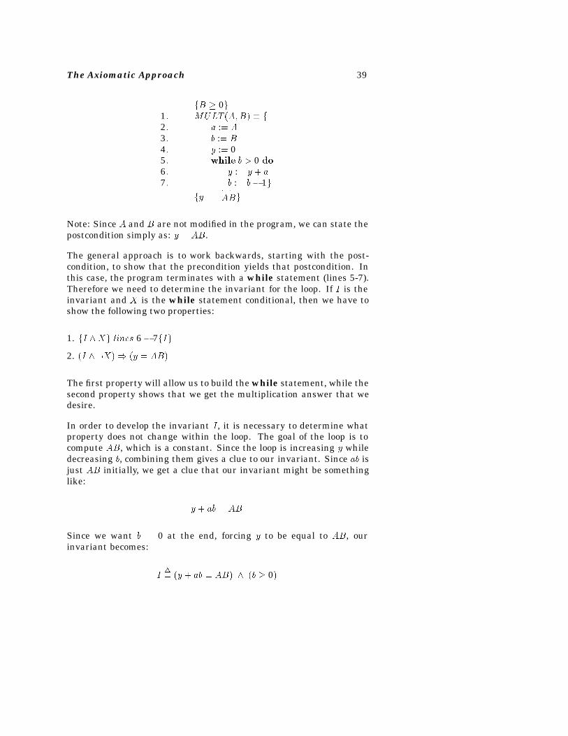
The Axiomatic Approach 39
fB � 0g1� MULT �A�B� � f2� a :� A3� b :� B4� y :� 05� while b � 0 do6� y :� y � a7� b :� b� 1g
fy ��
A�
Bg
Note: Since A and B are not modified in the program, we can state thepostcondition simply as: y � AB.
The general approach is to work backwards, starting with the post-condition, to show that the precondition yields that postcondition. Inthis case, the program terminates with a while statement (lines 5-7).Therefore we need to determine the invariant for the loop. If I is theinvariant and X is the while statement conditional, then we have toshow the following two properties:
1. fI Xg lines 6� 7fIg
2. �I �X� �y � AB�
The first property will allow us to build the while statement, while thesecond property shows that we get the multiplication answer that wedesire.
In order to develop the invariant I, it is necessary to determine whatproperty does not change within the loop. The goal of the loop is tocompute AB, which is a constant. Since the loop is increasing y whiledecreasing b, combining them gives a clue to our invariant. Since ab isjust AB initially, we get a clue that our invariant might be somethinglike:
y � ab � AB
Since we want b � 0 at the end, forcing y to be equal to AB, ourinvariant becomes:
I�� �y � ab � AB� �b � 0�
40 Software Specifications
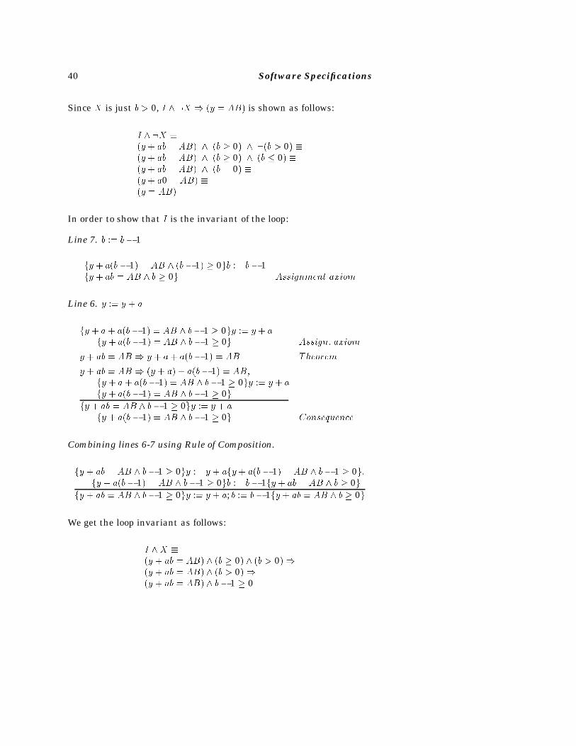
Since X is just b � 0, I �X �y � AB� is shown as follows:
I �X ��y � ab � AB� �b � 0� ��b � 0� ��y � ab � AB� �b � 0� �b � 0� ��y � ab � AB� �b � 0� ��y � a0 � AB� ��y � AB�
In order to show that I is the invariant of the loop:
Line 7. b :� b� 1
fy � a�b � 1� � AB �b� 1� � 0gb :� b� 1fy � ab � AB b � 0g Assignment axiom
Line 6. y :� y � a
fy � a � a�b� 1� � AB b� 1 � 0gy :� y � afy � a�b � 1� � AB b� 1 � 0g Assign� axiom
y � ab � AB y � a� a�b� 1� � AB Theorem
y � ab � AB �y � a� � a�b� 1� � AB�fy � a � a�b� 1� � AB b� 1 � 0gy :� y � afy � a�b � 1� � AB b� 1 � 0g
fy � ab � AB b� 1 � 0gy :� y � afy � a�b � 1� � AB b� 1 � 0g Consequence
Combining lines 6-7 using Rule of Composition.
fy � ab � AB b� 1 � 0gy :� y � afy � a�b� 1� � AB b� 1 � 0g�fy � a�b� 1� � AB b� 1 � 0gb :� b� 1fy � ab � AB b � 0g
fy � ab � AB b� 1 � 0gy :� y � a; b :� b� 1fy � ab � AB b � 0g
We get the loop invariant as follows:
I X ��y � ab � AB� �b � 0� �b � 0��y � ab � AB� �b � 0� �y � ab � AB� b� 1 � 0
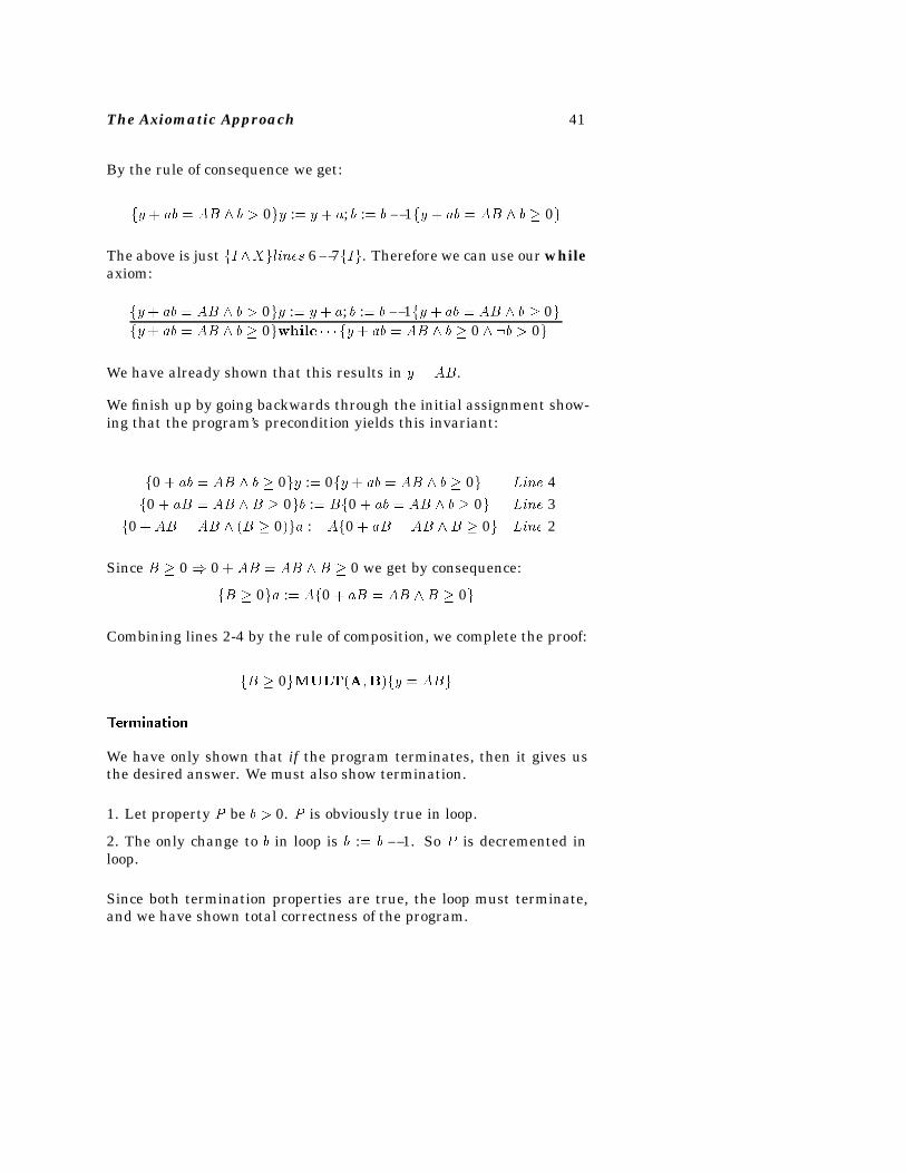
The Axiomatic Approach 41
By the rule of consequence we get:
fy � ab � AB b � 0gy :� y � a; b :� b� 1fy � ab � AB b � 0g
The above is just fIXglines 6�7fIg. Therefore we can use our whileaxiom:
fy � ab � AB b � 0gy :� y � a; b :� b� 1fy � ab � AB b � 0gfy � ab � AB b � 0gwhile � � � fy � ab � AB b � 0 �b � 0g
We have already shown that this results in y � AB.
We finish up by going backwards through the initial assignment show-ing that the program’s precondition yields this invariant:
f0 � ab � AB b � 0gy :� 0fy � ab � AB b � 0g Line 4f0 � aB � AB B � 0gb :� Bf0 � ab � AB b � 0g Line 3
f0 �AB � AB �B � 0�ga :� Af0 � aB � AB B � 0g Line 2
Since B � 0 0 � AB � AB B � 0 we get by consequence:
fB � 0ga :� Af0 � aB � AB B � 0g
Combining lines 2-4 by the rule of composition, we complete the proof:
fB � 0gMULT�A�B�fy � ABg
Termination
We have only shown that if the program terminates, then it gives usthe desired answer. We must also show termination.
1. Let property P be b � 0. P is obviously true in loop.
2. The only change to b in loop is b :� b � 1. So P is decremented inloop.
Since both termination properties are true, the loop must terminate,and we have shown total correctness of the program.
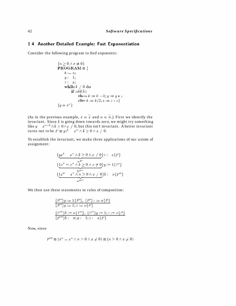
42 Software Specifications
���� Another Detailed Example� Fast Exponentiation
Consider the following program to find exponents:
fn � 0 x �� 0gPROGRAM � f
k :� n;y :� 1;z :� x;while k �� 0 do
if odd�k�then k :� k � 1; y :� y � zelse k :� k2; z :� z � zg
fy � xng
(As in the previous example, x ��x and n �
�n .) First we identify the
invariant. Since k is going down towards zero, we might try somethinglike y � xn�kk � 0x �� 0, but this isn’t invariant. A better invariantturns out to be P � yzk � xn k � 0 x �� 0.
To establish the invariant, we make three applications of our axiom ofassignment:
fyxk � xn k � 0 x �� 0� �z ��P �
gz :� xfPg
f1xk � xn k � 0 x �� 0� �z ��P ��
gy :� 1fP �g
f1xn � xn n � 0 x �� 0� �z ��P ���
gk :� nfP ��g
We then use these statements in rules of composition:
fP ��gy :� 1fP �g� fP �gz :� xfPgfP ��gy :� 1; z :� xfPg
fP ���gk :� nfP ��g� fP ��gy :� 1; z :� xfPg
fP ���gk :� n; y :� 1; z :� xfPg
Now, since
P ��� � �xn � xn n � 0 x �� 0� � �n � 0 x �� 0�
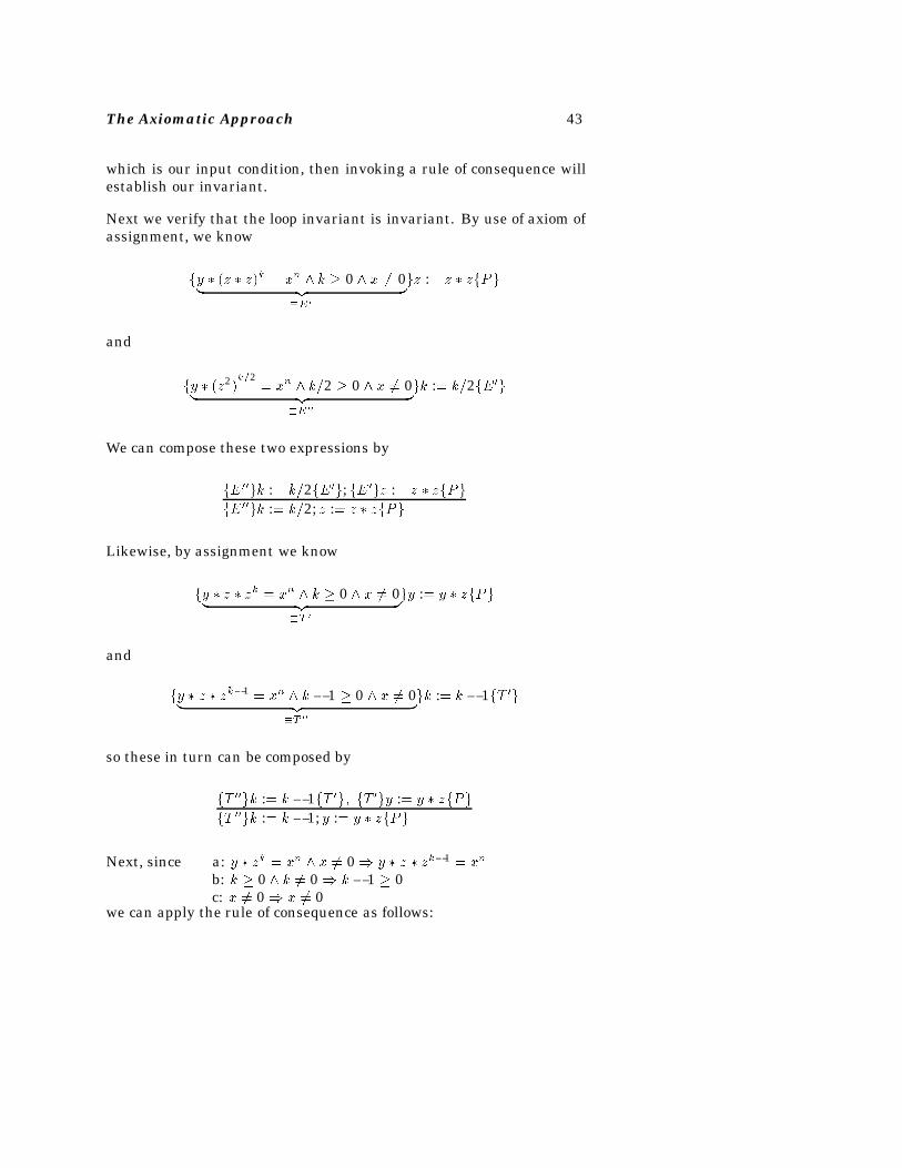
The Axiomatic Approach 43
which is our input condition, then invoking a rule of consequence willestablish our invariant.
Next we verify that the loop invariant is invariant. By use of axiom ofassignment, we know
fy � �z � z�k � xn k � 0 x �� 0� �z ��E�
gz :� z � zfPg
and
fy � �z2�k�2
� xn k2 � 0 x �� 0� �z ��E��
gk :� k2fE�g
We can compose these two expressions by
fE��gk :� k2fE�g; fE�gz :� z � zfPg
fE��gk :� k2; z :� z � zfPg
Likewise, by assignment we know
fy � z � zk � xn k � 0 x �� 0� �z ��T �
gy :� y � zfPg
and
fy � z � zk�1 � xn k � 1 � 0 x �� 0� �z ��T ��
gk :� k � 1fT �g
so these in turn can be composed by
fT ��gk :� k � 1fT �g� fT �gy :� y � zfPg
fT ��gk :� k � 1; y :� y � zfPg
Next, since a: y � zk � xn x �� 0 y � z � zk�1 � xn
b: k � 0 k �� 0 k � 1 � 0c: x �� 0 x �� 0
we can apply the rule of consequence as follows:
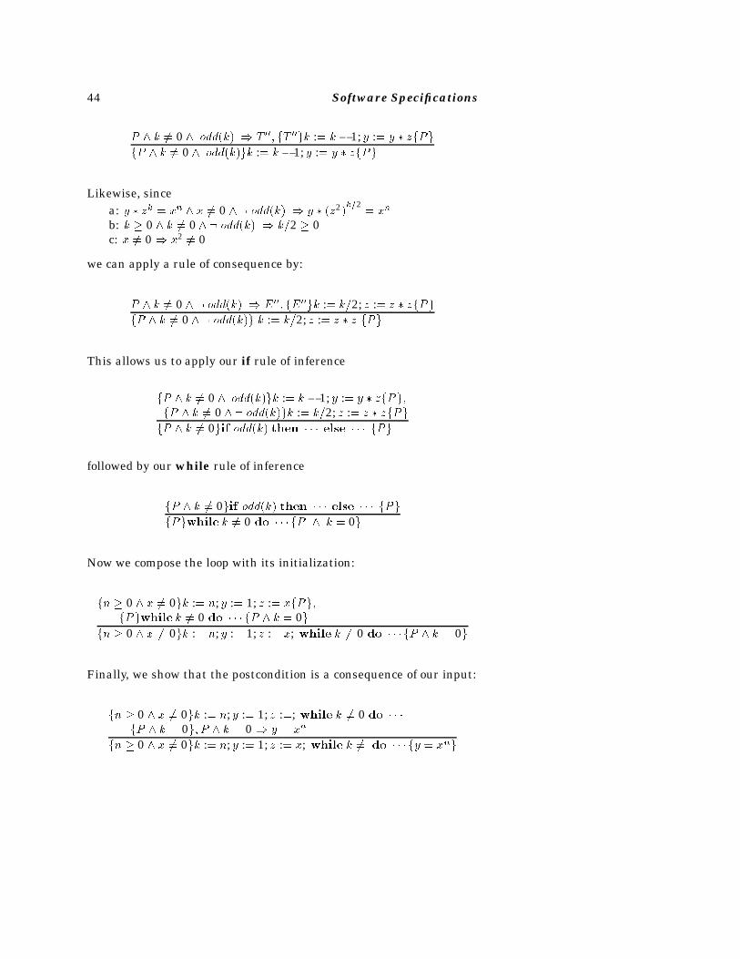
44 Software Specifications
P k �� 0 odd�k� T ��� fT ��gk :� k � 1; y :� y � zfPg
fP k �� 0 odd�k�gk :� k � 1; y :� y � zfPg
Likewise, sincea: y � zk � xn x �� 0 � odd�k� y � �z2�
k�2� xn
b: k � 0 k �� 0 � odd�k� k2 � 0c: x �� 0 x2 �� 0
we can apply a rule of consequence by:
P k �� 0 � odd�k� E��� fE��gk :� k2; z :� z � zfPgfP k �� 0 � odd�k�g k :� k2; z :� z � z fPg
This allows us to apply our if rule of inference
fP k �� 0 odd�k�gk :� k � 1; y :� y � zfPg�fP k �� 0 � odd�k�gk :� k2; z :� z � zfPg
fP k �� 0gif odd�k� then � � � else � � � fPg
followed by our while rule of inference
fP k �� 0gif odd�k� then � � � else � � � fPg
fPgwhile k �� 0 do � � � fP k � 0g
Now we compose the loop with its initialization:
fn � 0 x �� 0gk :� n; y :� 1; z :� xfPg�fPgwhile k �� 0 do � � � fP k � 0g
fn � 0 x �� 0gk :� n; y :� 1; z :� x; while k �� 0 do � � � fP k � 0g
Finally, we show that the postcondition is a consequence of our input:
fn � 0 x �� 0gk :� n; y :� 1; z :�; while k �� 0 do � � �fP k � 0g� P k � 0 y � xn
fn � 0 x �� 0gk :� n; y :� 1; z :� x; while k �� do � � � fy � xng
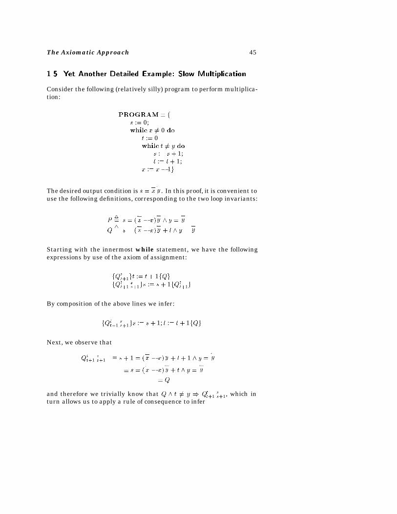
The Axiomatic Approach 45
���� Yet Another Detailed Example� Slow Multiplication
Consider the following (relatively silly) program to perform multiplica-tion:
PROGRAM � fs :� 0;while x �� 0 do
t :� 0while t �� y do
s :� s � 1;t :� t� 1;
x :� x� 1g
The desired output condition is s ��x�y . In this proof, it is convenient to
use the following definitions, corresponding to the two loop invariants:
P�� s � �
�x � x�
�y y �
�y
Q�� s � �
�x � x�
�y � t y �
�y
Starting with the innermost while statement, we have the followingexpressions by use of the axiom of assignment:
fQtt�1gt :� t� 1fQg
fQtt�1
ss�1gs :� s � 1fQt
t�1g
By composition of the above lines we infer:
fQtt�1
ss�1gs :� s � 1; t :� t � 1fQg
Next, we observe that
Qtt�1
ss�1 � s � 1 � �
�x � x�
�y � t� 1 y �
�y
� s � ��x � x�
�y � t y �
�y
� Q
and therefore we trivially know that Q t �� y Qtt�1ss�1, which in
turn allows us to apply a rule of consequence to infer
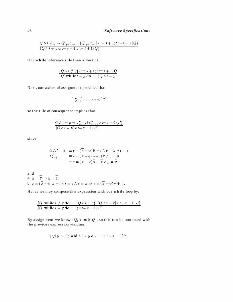
46 Software Specifications
Q t �� y Qtt�1
ss�1 � fQ
tt�1
ss�1gs :� s � 1; t :� t� 1fQg
fQ t �� ygs :� s � 1; t :� t � 1fQg
Our while inference rule then allows us
fQ t �� ygs :� s� 1; t :� t� 1fQgfQgwhile t �� y do � � � fQ t � yg
Next, our axiom of assignment provides that
fP xx�1gx :� x� 1fPg
so the rule of consequence implies that
Q t � y P xx�1� fP
xx�1gx :� x� 1fPg
fQ t � ygx :� x� 1fPg
since
Q t � y � s � ��x � x�
�y � t y �
�y t � y
P xx�1 � s � �
�x � �x� 1��
�y y �
�y
� s � ��x � x�
�y �
�y y �
�y
anda: y �
�y y �
�y .
b: s � ��x � x�
�y � t t � y y �
�y s � �
�x � x�
�y �
�y .
Hence we may compose this expression with our while loop by:
fQgwhile t �� y do � � � fQ t � yg� fQ t � ygx :� x� 1fPgfQgwhile t �� y do � � � ;x :� x� 1fPg
By assignment we know fQt0gt :� 0fQg, so this can be composed withthe previous expression yielding:
fQt0gt :� 0; while t �� y do � � � ;x :� x� 1fPg
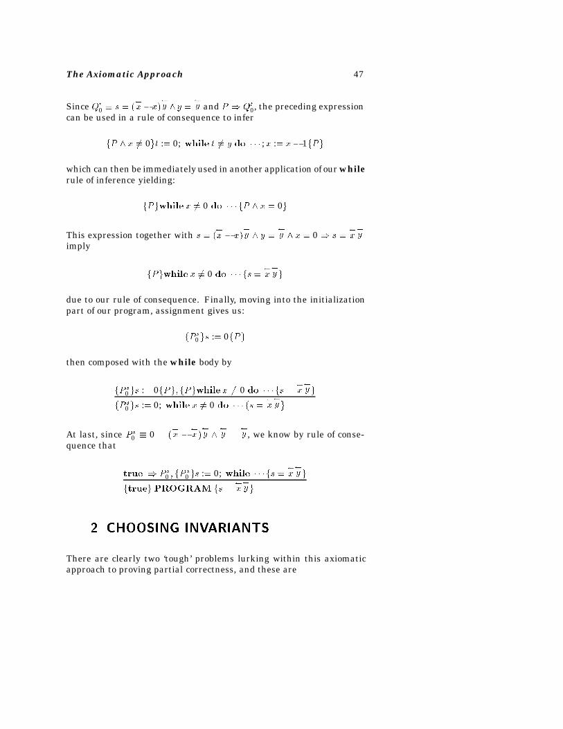
The Axiomatic Approach 47
Since Qt0 � s � �
�x �x�
�y y �
�y and P Qt
0, the preceding expressioncan be used in a rule of consequence to infer
fP x �� 0gt :� 0; while t �� y do � � � ;x :� x� 1fPg
which can then be immediately used in another application of our whilerule of inference yielding:
fPgwhile x �� 0 do � � � fP x � 0g
This expression together with s � ��x � x�
�y y �
�y x � 0 s �
�x�y
imply
fPgwhile x �� 0 do � � � fs ��x�y g
due to our rule of consequence. Finally, moving into the initializationpart of our program, assignment gives us:
fP s0 gs :� 0fPg
then composed with the while body by
fP s0 gs :� 0fPg� fPgwhile x �� 0 do � � � fs �
�x�y g
fP s0 gs :� 0; while x �� 0 do � � � fs �
�x�y g
At last, since Ps0 � 0 � �
�x �
�x�
�y
�y �
�y , we know by rule of conse-
quence that
true P s0 � fP
s0 gs :� 0; while � � � fs �
�x�y g
ftrueg PROGRAM fs ��x�y g
�� CHOOSING INVARIANTS
There are clearly two ‘tough’ problems lurking within this axiomaticapproach to proving partial correctness, and these are
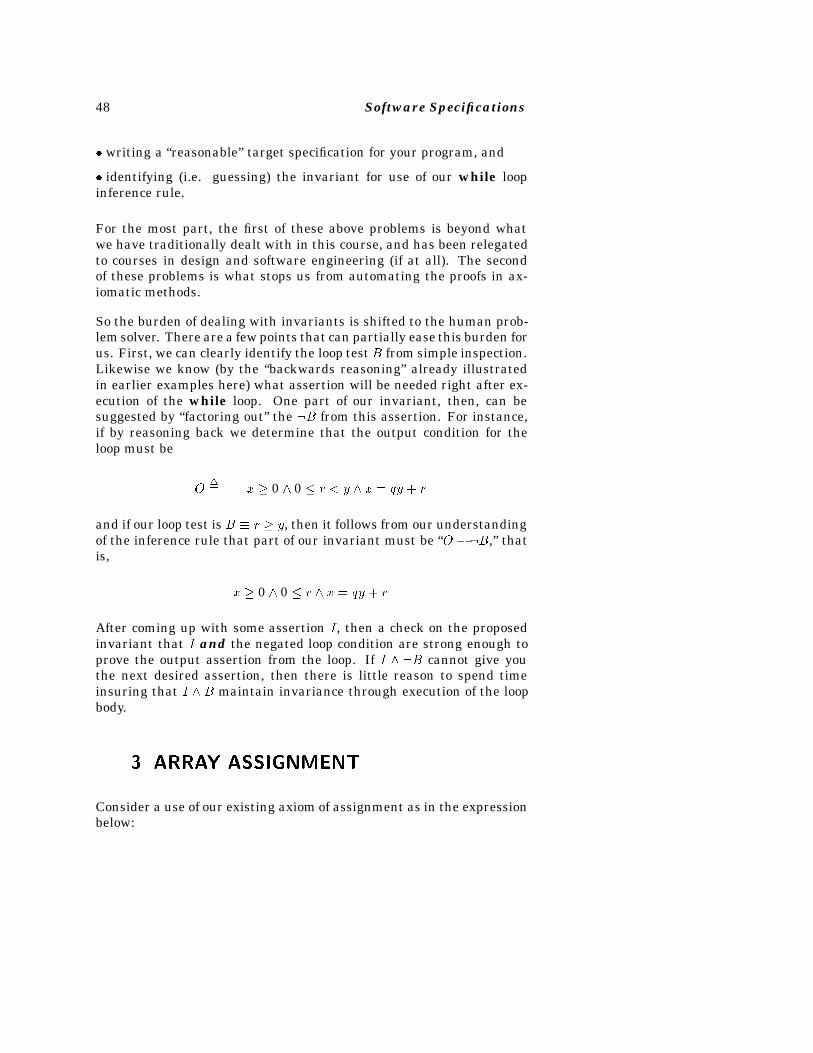
48 Software Specifications
� writing a “reasonable” target specification for your program, and
� identifying (i.e. guessing) the invariant for use of our while loopinference rule.
For the most part, the first of these above problems is beyond whatwe have traditionally dealt with in this course, and has been relegatedto courses in design and software engineering (if at all). The secondof these problems is what stops us from automating the proofs in ax-iomatic methods.
So the burden of dealing with invariants is shifted to the human prob-lem solver. There are a few points that can partially ease this burden forus. First, we can clearly identify the loop testB from simple inspection.Likewise we know (by the “backwards reasoning” already illustratedin earlier examples here) what assertion will be needed right after ex-ecution of the while loop. One part of our invariant, then, can besuggested by “factoring out” the �B from this assertion. For instance,if by reasoning back we determine that the output condition for theloop must be
O�� x � 0 0 � r � y x � qy � r
and if our loop test is B � r � y, then it follows from our understandingof the inference rule that part of our invariant must be “O ��B,” thatis,
x � 0 0 � r x � qy � r
After coming up with some assertion I, then a check on the proposedinvariant that I and the negated loop condition are strong enough toprove the output assertion from the loop. If I �B cannot give youthe next desired assertion, then there is little reason to spend timeinsuring that I B maintain invariance through execution of the loopbody.
�� ARRAY ASSIGNMENT
Consider a use of our existing axiom of assignment as in the expressionbelow:
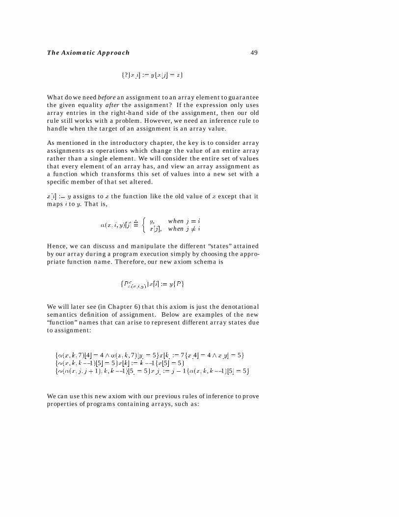
The Axiomatic Approach 49
f?gx�i� :� yfx�j� � zg
What do we need before an assignment to an array element to guaranteethe given equality after the assignment? If the expression only usesarray entries in the right-hand side of the assignment, then our oldrule still works with a problem. However, we need an inference rule tohandle when the target of an assignment is an array value.
As mentioned in the introductory chapter, the key is to consider arrayassignments as operations which change the value of an entire arrayrather than a single element. We will consider the entire set of valuesthat every element of an array has, and view an array assignment asa function which transforms this set of values into a new set with aspecific member of that set altered.
x�i� :� y assigns to x the function like the old value of x except that itmaps i to y. That is,
��x� i� y��j���
�y, when j � ix�j�, when j �� i
Hence, we can discuss and manipulate the different “states” attainedby our array during a program execution simply by choosing the appro-priate function name. Therefore, our new axiom schema is
fP x��x�i�y�gx�i� :� yfPg
We will later see (in Chapter 6) that this axiom is just the denotationalsemantics definition of assignment. Below are examples of the new“function” names that can arise to represent different array states dueto assignment:
f��x� k� 7��4� � 4 ��x� k� 7��y� � 5gx�k� :� 7fx�4� � 4 x�y� � 5gf��x� k� k� 1��5� � 5gx�k� :� k � 1fx�5� � 5gf����x� j� j � 1�� k� k� 1��5� � 5gx�j� :� j � 1f��x� k� k� 1��5� � 5g
We can use this new axiom with our previous rules of inference to proveproperties of programs containing arrays, such as:
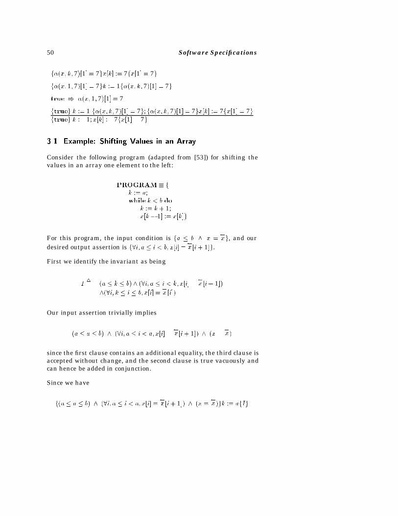
50 Software Specifications
f��x� k� 7��1� � 7gx�k� :� 7fx�1� � 7g
f��x� 1� 7��1� � 7gk :� 1f��x� k� 7��1� � 7g
true ��x� 1� 7��1� � 7
ftrueg k :� 1 f��x� k� 7��1� � 7g; f��x� k� 7��1� � 7gx�k� :� 7fx�1� � 7gftrueg k :� 1;x�k� :� 7fx�1� � 7g
���� Example� Shifting Values in an Array
Consider the following program (adapted from [53]) for shifting thevalues in an array one element to the left:
PROGRAM � fk :� a;while k � b do
k :� k � 1;x�k� 1� :� x�k�g
For this program, the input condition is fa � b x ��xg, and our
desired output assertion is f�i� a � i � b� x�i� ��x �i� 1�g.
First we identify the invariant as being
I�� �a � k � b� ��i� a � i � k� x�i� �
�x �i� 1��
��i� k � i � b� x�i� ��x �i��
Our input assertion trivially implies
�a � a � b� ��i� a � i � a� x�i� ��x �i� 1�� �x �
�x�
since the first clause contains an additional equality, the third clause isaccepted without change, and the second clause is true vacuously andcan hence be added in conjunction.
Since we have
f�a � a � b� ��i� a � i � a� x�i� ��x �i� 1�� �x �
�x �gk :� afIg
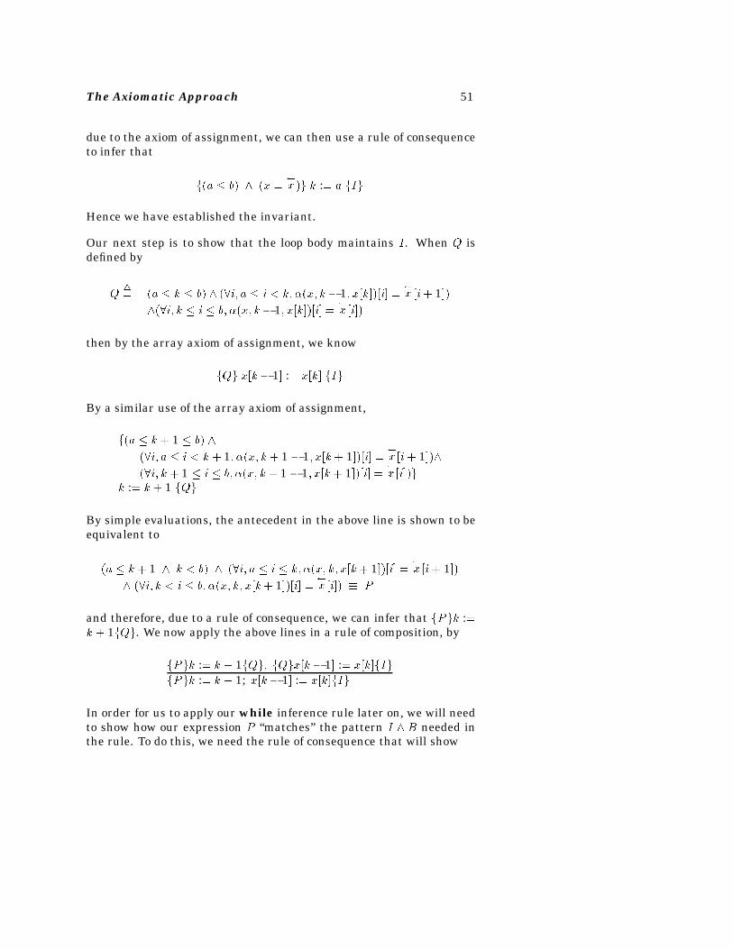
The Axiomatic Approach 51
due to the axiom of assignment, we can then use a rule of consequenceto infer that
f�a � b� �x ��x�g k :� a fIg
Hence we have established the invariant.
Our next step is to show that the loop body maintains I. When Q isdefined by
Q�� �a � k � b� ��i� a � i � k� ��x� k� 1� x�k���i� �
�x �i� 1��
��i� k � i � b� ��x� k� 1� x�k���i� ��x �i��
then by the array axiom of assignment, we know
fQg x�k� 1� :� x�k� fIg
By a similar use of the array axiom of assignment,
f�a � k � 1 � b�
��i� a � i � k � 1� ��x� k� 1 � 1� x�k� 1���i� ��x �i� 1��
��i� k � 1 � i � b� ��x� k� 1 � 1� x�k� 1���i� ��x �i��g
k :� k � 1 fQg
By simple evaluations, the antecedent in the above line is shown to beequivalent to
�a � k � 1 k � b� ��i� a � i � k� ��x� k� x�k� 1���i� ��x �i� 1��
��i� k � i � b� ��x� k� x�k� 1���i� ��x �i�� � P
and therefore, due to a rule of consequence, we can infer that fPgk :�k � 1fQg. We now apply the above lines in a rule of composition, by
fPgk :� k � 1fQg� fQgx�k� 1� :� x�k�fIgfPgk :� k � 1; x�k� 1� :� x�k�fIg
In order for us to apply our while inference rule later on, we will needto show how our expression P “matches” the pattern I B needed inthe rule. To do this, we need the rule of consequence that will show
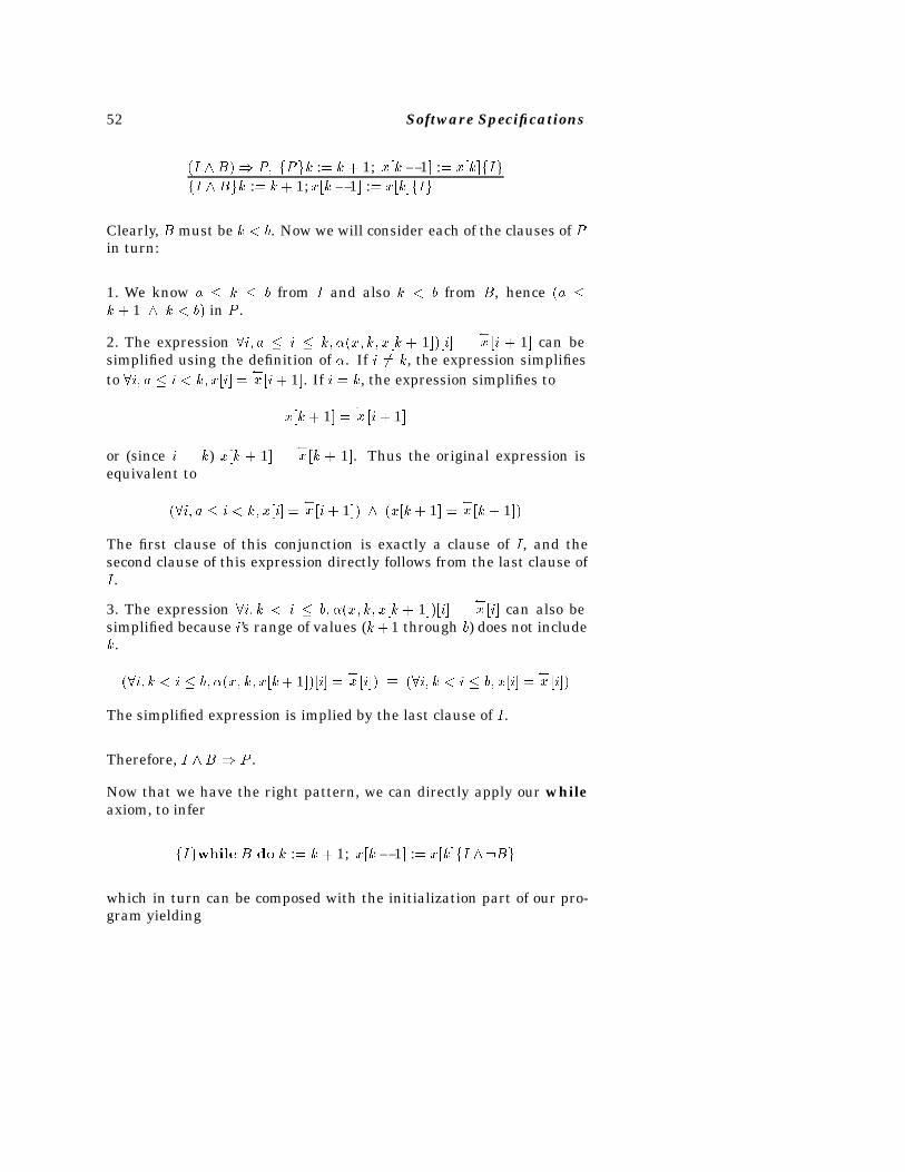
52 Software Specifications
�I B� P� fPgk :� k � 1; x�k� 1� :� x�k�fIg
fI Bgk :� k � 1;x�k� 1� :� x�k�fIg
Clearly, B must be k � b. Now we will consider each of the clauses of Pin turn:
1. We know a � k � b from I and also k � b from B, hence �a �k � 1 k � b� in P .
2. The expression �i� a � i � k� ��x� k� x�k � 1���i� ��x �i � 1� can be
simplified using the definition of �. If i �� k, the expression simplifiesto �i� a � i � k� x�i� �
�x �i� 1�. If i � k, the expression simplifies to
x�k� 1� ��x �i� 1�
or (since i � k) x�k � 1� ��x �k � 1�. Thus the original expression is
equivalent to
��i� a � i � k� x�i� ��x �i� 1�� �x�k� 1� �
�x �k� 1��
The first clause of this conjunction is exactly a clause of I, and thesecond clause of this expression directly follows from the last clause ofI.
3. The expression �i� k � i � b� ��x� k� x�k � 1���i� ��x �i� can also be
simplified because i’s range of values (k� 1 through b) does not includek.
��i� k � i � b� ��x� k� x�k� 1���i� ��x �i�� � ��i� k � i � b� x�i� �
�x �i��
The simplified expression is implied by the last clause of I.
Therefore, I B P .
Now that we have the right pattern, we can directly apply our whileaxiom, to infer
fIgwhile B do k :� k � 1; x�k� 1� :� x�k�fI �Bg
which in turn can be composed with the initialization part of our pro-gram yielding
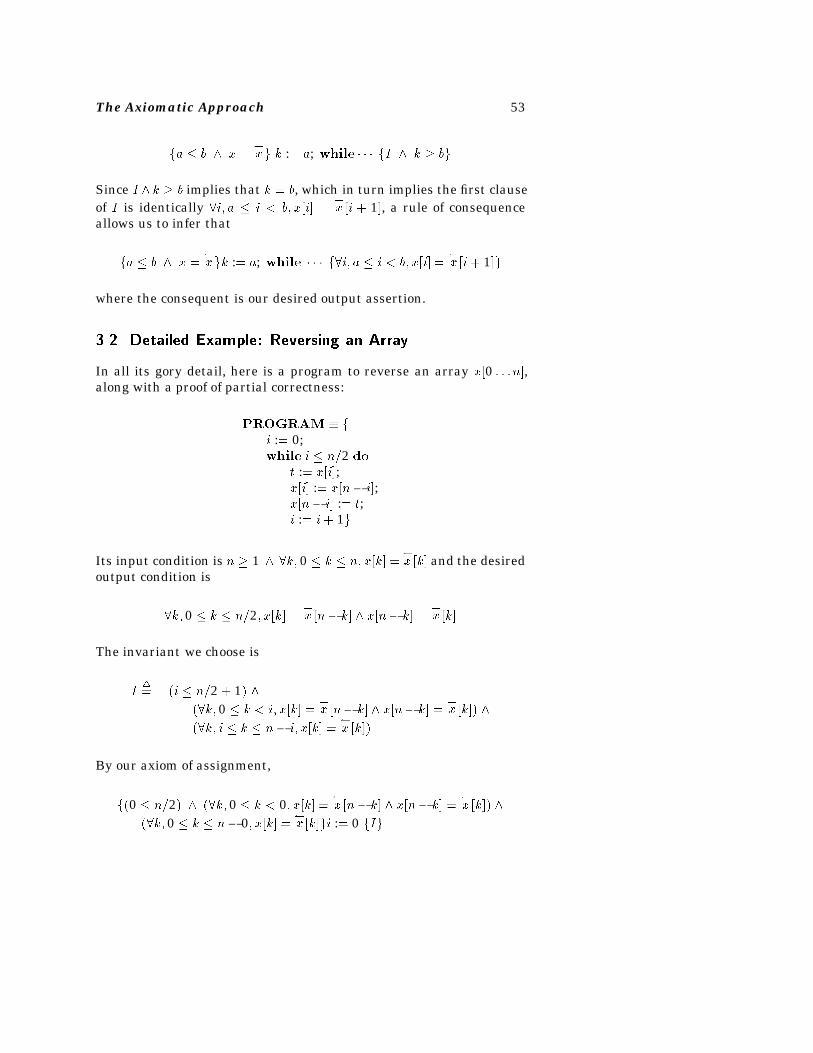
The Axiomatic Approach 53
fa � b x ��xg k :� a; while � � � fI k � bg
Since I k � b implies that k � b, which in turn implies the first clauseof I is identically �i� a � i � b� x�i� �
�x �i � 1�, a rule of consequence
allows us to infer that
fa � b x ��xgk :� a; while � � � f�i� a � i � b� x�i� �
�x �i� 1�g
where the consequent is our desired output assertion.
���� Detailed Example� Reversing an Array
In all its gory detail, here is a program to reverse an array x�0 � � �n�,along with a proof of partial correctness:
PROGRAM � fi :� 0;while i � n2 do
t :� x�i�;x�i� :� x�n� i�;x�n� i� :� t;i :� i� 1g
Its input condition is n � 1 �k� 0 � k � n� x�k� ��x �k� and the desired
output condition is
�k� 0 � k � n2� x�k� ��x �n� k� x�n� k� �
�x �k�
The invariant we choose is
I�� �i � n2 � 1�
��k� 0 � k � i� x�k� ��x �n� k� x�n� k� �
�x �k��
��k� i � k � n� i� x�k� ��x �k��
By our axiom of assignment,
f�0 � n2� ��k� 0 � k � 0� x�k� ��x �n� k� x�n� k� �
�x �k��
��k� 0 � k � n� 0� x�k� ��x �k�gi :� 0 fIg
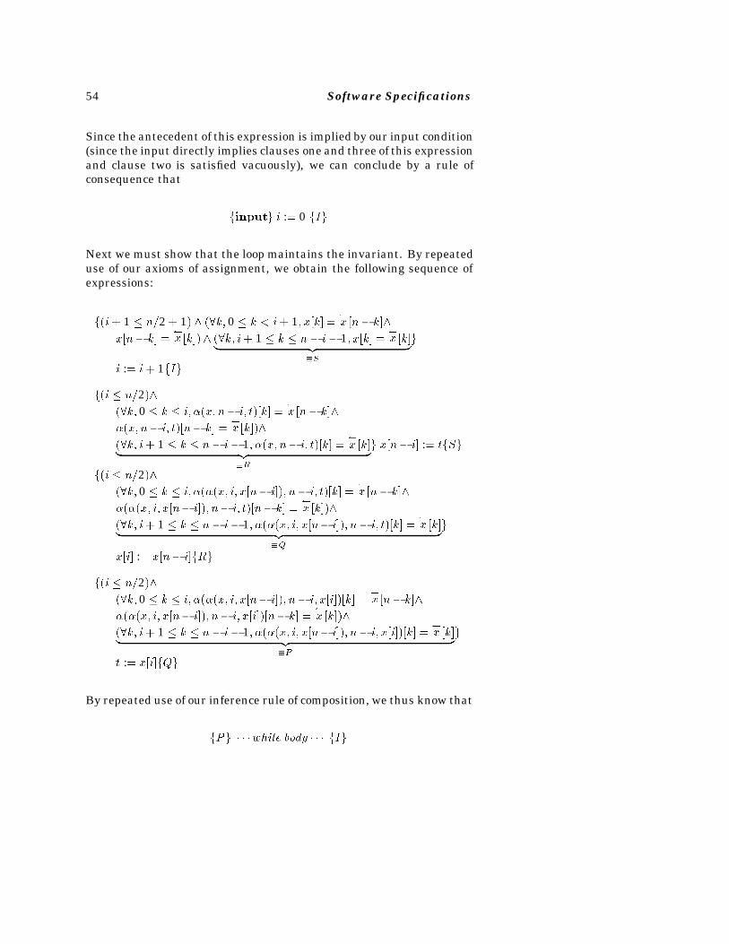
54 Software Specifications
Since the antecedent of this expression is implied by our input condition(since the input directly implies clauses one and three of this expressionand clause two is satisfied vacuously), we can conclude by a rule ofconsequence that
finputg i :� 0 fIg
Next we must show that the loop maintains the invariant. By repeateduse of our axioms of assignment, we obtain the following sequence ofexpressions:
f�i � 1 � n2 � 1� ��k� 0 � k � i� 1� x�k� ��x �n� k�
x�n� k� ��x �k�� ��k� i� 1 � k � n � i � 1� x�k� �
�x �k�� �z �
�S
g
i :� i � 1fIg
f�i � n2���k� 0 � k � i� ��x� n� i� t��k� �
�x �n� k�
��x� n� i� t��n� k� ��x �k��
��k� i� 1 � k � n � i � 1� ��x� n� i� t��k� ��x �k�� �z �
�R
g x�n� i� :� tfSg
f�i � n2���k� 0 � k � i� ����x� i� x�n� i��� n� i� t��k� �
�x �n� k�
����x� i� x�n� i��� n� i� t��n� k� ��x �k��
��k� i� 1 � k � n � i � 1� ����x� i� x�n� i��� n� i� t��k� ��x �k�� �z �
�Q
g
x�i� :� x�n� i�fRg
f�i � n2���k� 0 � k � i� ����x� i� x�n� i��� n� i� x�i���k� �
�x �n� k�
����x� i� x�n� i��� n� i� x�i���n� k� ��x �k��
��k� i� 1 � k � n � i � 1� ����x� i� x�n� i��� n� i� x�i���k� ��x �k�� �z �
�P
g
t :� x�i�fQg
By repeated use of our inference rule of composition, we thus know that
fPg � � �while body � � � fIg
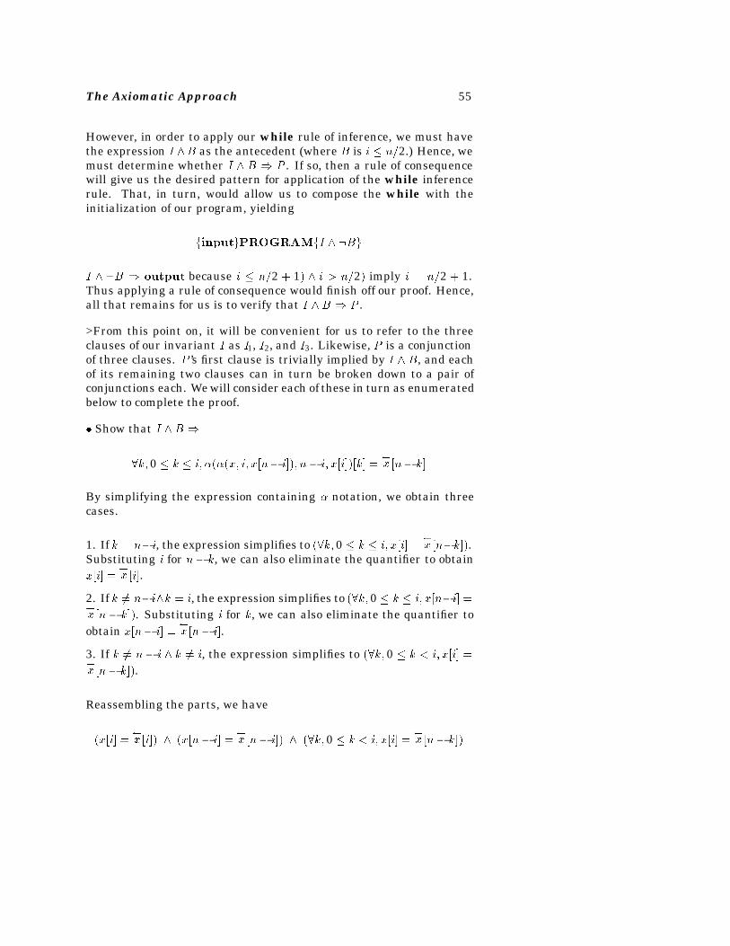
The Axiomatic Approach 55
However, in order to apply our while rule of inference, we must havethe expression I B as the antecedent (where B is i � n2.) Hence, wemust determine whether I B P . If so, then a rule of consequencewill give us the desired pattern for application of the while inferencerule. That, in turn, would allow us to compose the while with theinitialization of our program, yielding
finputgPROGRAMfI �Bg
I �B output because i � n2 � 1� i � n2� imply i � n2 � 1.Thus applying a rule of consequence would finish off our proof. Hence,all that remains for us is to verify that I B P .
>From this point on, it will be convenient for us to refer to the threeclauses of our invariant I as I1, I2, and I3. Likewise, P is a conjunctionof three clauses. P ’s first clause is trivially implied by I B, and eachof its remaining two clauses can in turn be broken down to a pair ofconjunctions each. We will consider each of these in turn as enumeratedbelow to complete the proof.
� Show that I B
�k� 0 � k � i� ����x� i� x�n� i��� n� i� x�i���k� ��x �n� k�
By simplifying the expression containing � notation, we obtain threecases.
1. If k � n�i, the expression simplifies to ��k� 0 � k � i� x�i� ��x �n�k��.
Substituting i for n� k, we can also eliminate the quantifier to obtainx�i� �
�x �i�.
2. If k �� n�ik � i, the expression simplifies to ��k� 0 � k � i� x�n�i� ��x �n � k��. Substituting i for k, we can also eliminate the quantifier toobtain x�n� i� �
�x �n� i�.
3. If k �� n� i k �� i, the expression simplifies to ��k� 0 � k � i� x�i� ��x �n� k��.
Reassembling the parts, we have
�x�i� ��x �i�� �x�n� i� �
�x �n� i�� ��k� 0 � k � i� x�i� �
�x �n� k��
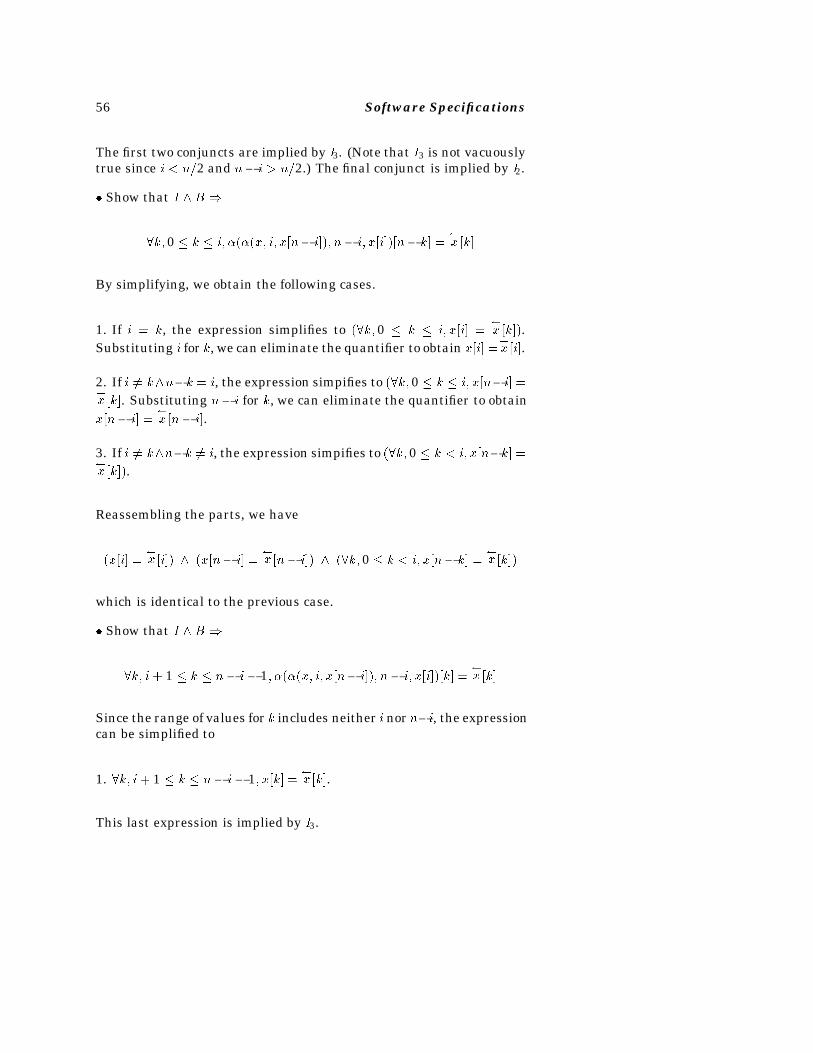
56 Software Specifications
The first two conjuncts are implied by I3. (Note that I3 is not vacuouslytrue since i � n2 and n� i � n2.) The final conjunct is implied by I2.
� Show that I B
�k� 0 � k � i� ����x� i� x�n� i��� n� i� x�i���n� k� ��x �k�
By simplifying, we obtain the following cases.
1. If i � k, the expression simplifies to ��k� 0 � k � i� x�i� ��x �k��.
Substituting i for k, we can eliminate the quantifier to obtain x�i� ��x �i�.
2. If i �� kn�k � i, the expression simpifies to ��k� 0 � k � i� x�n�i� ��x �k�. Substituting n� i for k, we can eliminate the quantifier to obtainx�n� i� �
�x �n� i�.
3. If i �� kn�k �� i, the expression simpifies to ��k� 0 � k � i� x�n�k� ��x �k��.
Reassembling the parts, we have
�x�i� ��x �i�� �x�n� i� �
�x �n� i�� ��k� 0 � k � i� x�n� k� �
�x �k��
which is identical to the previous case.
� Show that I B
�k� i� 1 � k � n � i � 1� ����x� i� x�n� i��� n� i� x�i���k� ��x �k�
Since the range of values for k includes neither i nor n�i, the expressioncan be simplified to
1. �k� i� 1 � k � n� i� 1� x�k� ��x �k�.
This last expression is implied by I3.
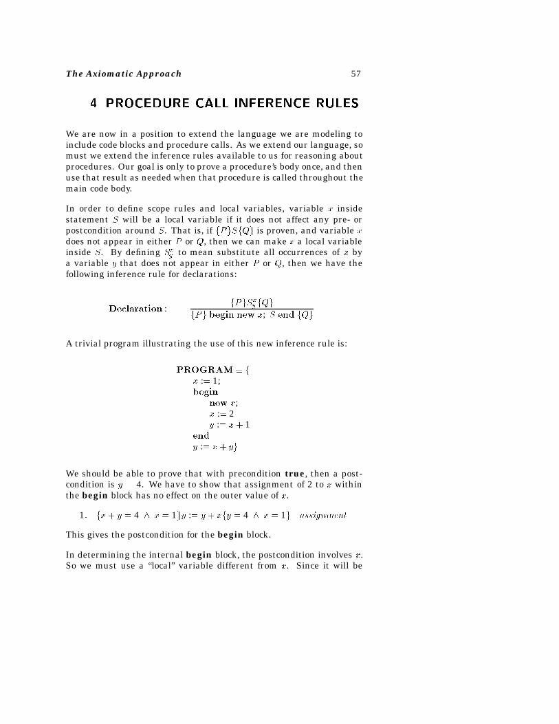
The Axiomatic Approach 57
�� PROCEDURE CALL INFERENCE RULES
We are now in a position to extend the language we are modeling toinclude code blocks and procedure calls. As we extend our language, somust we extend the inference rules available to us for reasoning aboutprocedures. Our goal is only to prove a procedure’s body once, and thenuse that result as needed when that procedure is called throughout themain code body.
In order to define scope rules and local variables, variable x insidestatement S will be a local variable if it does not affect any pre- orpostcondition around S. That is, if fPgSfQg is proven, and variable xdoes not appear in either P or Q, then we can make x a local variableinside S. By defining Sxy to mean substitute all occurrences of x bya variable y that does not appear in either P or Q, then we have thefollowing inference rule for declarations:
Declaration :fPgSxyfQg
fPg begin new x; S end fQg
A trivial program illustrating the use of this new inference rule is:
PROGRAM � fx :� 1;begin
new x;x :� 2y :� x� 1
end
y :� x� yg
We should be able to prove that with precondition true, then a post-condition is y � 4. We have to show that assignment of 2 to x withinthe begin block has no effect on the outer value of x.
1� fx� y � 4 x � 1gy :� y � xfy � 4 x � 1g assignment
This gives the postcondition for the begin block.
In determining the internal begin block, the postcondition involves x.So we must use a “local” variable different from x. Since it will be
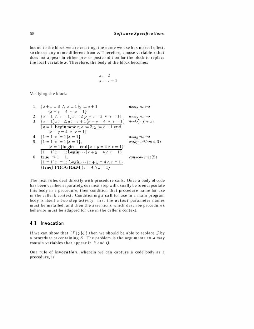
58 Software Specifications
bound to the block we are creating, the name we use has no real effect,so choose any name different from x. Therefore, choose variable z thatdoes not appear in either pre- or postcondition for the block to replacethe local variable x. Therefore, the body of the block becomes:
z :� 2y :� z � 1
Verifying the block:
1� fx� z � 3 x � 1gy :� z � 1 assignmentfx� y � 4 x � 1g
2� fx � 1 x � 1gz :� 2fx� z � 3 x � 1g assignment3� fx � 1gz :� 2; y :� z � 1fx� y � 4 x � 1g decl��x for z�
fx � 1gbegin new x;x :� 2; y :� x� 1 endfx� y � 4 x � 1g
4� f1 � 1gx :� 1fx � 1g assignment5� f1 � 1gx :� 1fx � 1g� composition�4� 3�
fx � 1gbegin � � �endfx� y � 4 x � 1gf1 � 1gx :� 1;begin � � � fx� y � 4 x � 1g
6� true 1 � 1� consequence�5�f1 � 1gx :� 1; begin � � � fx� y � 4 x � 1gftrueg PROGRAM fy � 4 x � 1g
The next rules deal directly with procedure calls. Once a body of codehas been verified separately, our next step will usually be to encapsulatethis body in a procedure, then condition that procedure name for usein the caller’s context. Conditioning a call for use in a main programbody is itself a two step activity: first the actual parameter namesmust be installed, and then the assertions which describe procedure’sbehavior must be adapted for use in the caller’s context.
���� Invocation
If we can show that fPgSfQg then we should be able to replace S bya procedure containing S. The problem is the arguments to maycontain variables that appear in P and Q.
Our rule of invocation, wherein we can capture a code body as aprocedure, is
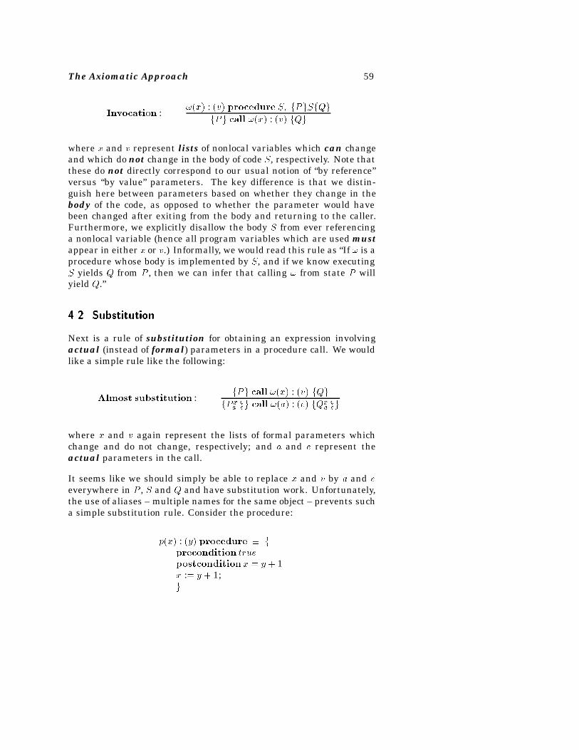
The Axiomatic Approach 59
Invocation :�x� : �v� procedure S� fPgSfQg
fPg call �x� : �v� fQg
where x and v represent lists of nonlocal variables which can changeand which do not change in the body of code S, respectively. Note thatthese do not directly correspond to our usual notion of “by reference”versus “by value” parameters. The key difference is that we distin-guish here between parameters based on whether they change in thebody of the code, as opposed to whether the parameter would havebeen changed after exiting from the body and returning to the caller.Furthermore, we explicitly disallow the body S from ever referencinga nonlocal variable (hence all program variables which are used mustappear in either x or v.) Informally, we would read this rule as “If is aprocedure whose body is implemented by S, and if we know executingS yields Q from P , then we can infer that calling from state P willyield Q.”
���� Substitution
Next is a rule of substitution for obtaining an expression involvingactual (instead of formal) parameters in a procedure call. We wouldlike a simple rule like the following:
Almost substitution :fPg call �x� : �v� fQg
fP xaveg call �a� : �e� fQx
aveg
where x and v again represent the lists of formal parameters whichchange and do not change, respectively; and a and e represent theactual parameters in the call.
It seems like we should simply be able to replace x and v by a and eeverywhere in P , S and Q and have substitution work. Unfortunately,the use of aliases – multiple names for the same object – prevents sucha simple substitution rule. Consider the procedure:
p�x� : �y� procedure � fprecondition truepostcondition x � y � 1x :� y � 1;g
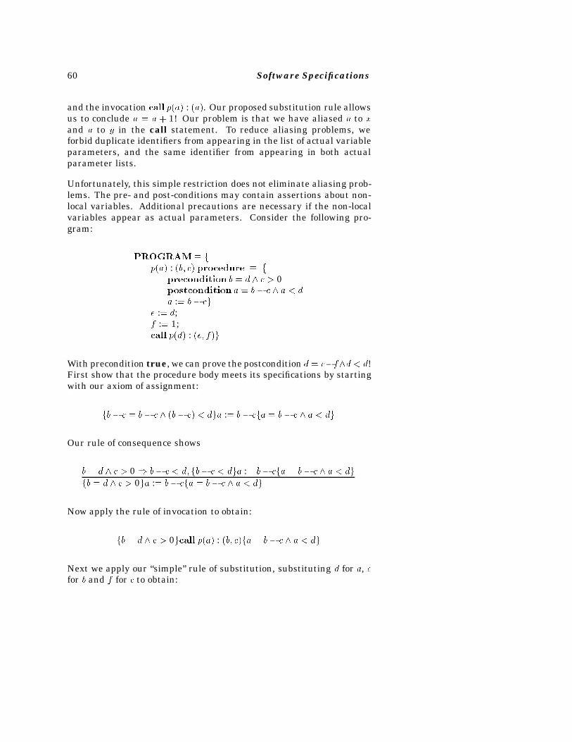
60 Software Specifications
and the invocation call p�a� : �a�. Our proposed substitution rule allowsus to conclude a � a � 1! Our problem is that we have aliased a to xand a to y in the call statement. To reduce aliasing problems, weforbid duplicate identifiers from appearing in the list of actual variableparameters, and the same identifier from appearing in both actualparameter lists.
Unfortunately, this simple restriction does not eliminate aliasing prob-lems. The pre- and post-conditions may contain assertions about non-local variables. Additional precautions are necessary if the non-localvariables appear as actual parameters. Consider the following pro-gram:
PROGRAM � fp�a� : �b� c� procedure � f
precondition b � d c � 0postcondition a � b � c a � da :� b� cg
e :� d;f :� 1;call p�d� : �e� f�g
With precondition true, we can prove the postcondition d � e�fd � d!First show that the procedure body meets its specifications by startingwith our axiom of assignment:
fb� c � b� c �b� c� � dga :� b� cfa � b� c a � dg
Our rule of consequence shows
b � d c � 0 b� c � d� fb� c � dga :� b� cfa � b� c a � dgfb � d c � 0ga :� b� cfa � b� c a � dg
Now apply the rule of invocation to obtain:
fb � d c � 0gcall p�a� : �b� c�fa � b� c a � dg
Next we apply our “simple” rule of substitution, substituting d for a, efor b and f for c to obtain:
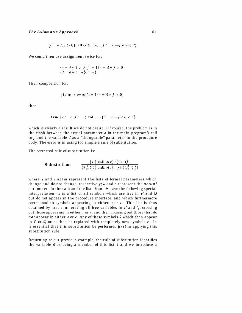
The Axiomatic Approach 61
fe � d f � 0gcall p�d� : �e� f�fd � e � f d � dg
We could then use assignment twice for:
fe � d 1 � 0gf :� 1fe � d f � 0gfd � dge :� dfe � dg
Then composition for:
ftrueg e :� d; f :� 1fe � d f � 0g
then
ftrueg e :� d; f :� 1; call � � � fd � e� f d � dg
which is clearly a result we do not desire. Of course, the problem is inthe clash between the actual parameter d in the main program’s callto p and the variable d as a “changeable” parameter in the procedurebody. The error is in using too simple a rule of substitution.
The corrected rule of substitution is:
Substitution :fPg call �x� : �v� fQg
fP kk�
xaveg call �a� : �e� fQk
k�
xaveg
where x and v again represent the lists of formal parameters whichchange and do not change, respectively; a and e represent the actualparameters in the call; and the lists k and k� have the following specialinterpretation: k is a list of all symbols which are free in P and Qbut do not appear in the procedure interface, and which furthermorecorrespond to symbols appearing in either a or e. This list is thusobtained by first enumerating all free variables in P and Q, crossingout those appearing in either x or v, and then crossing out those that donot appear in either a or e. Any of these symbols k which then appearin P or Q must then be replaced with completely new symbols k�. Itis essential that this substitution be performed first in applying thissubstitution rule.
Returning to our previous example, the rule of substitution identifiesthe variable d as being a member of this list k and we introduce a
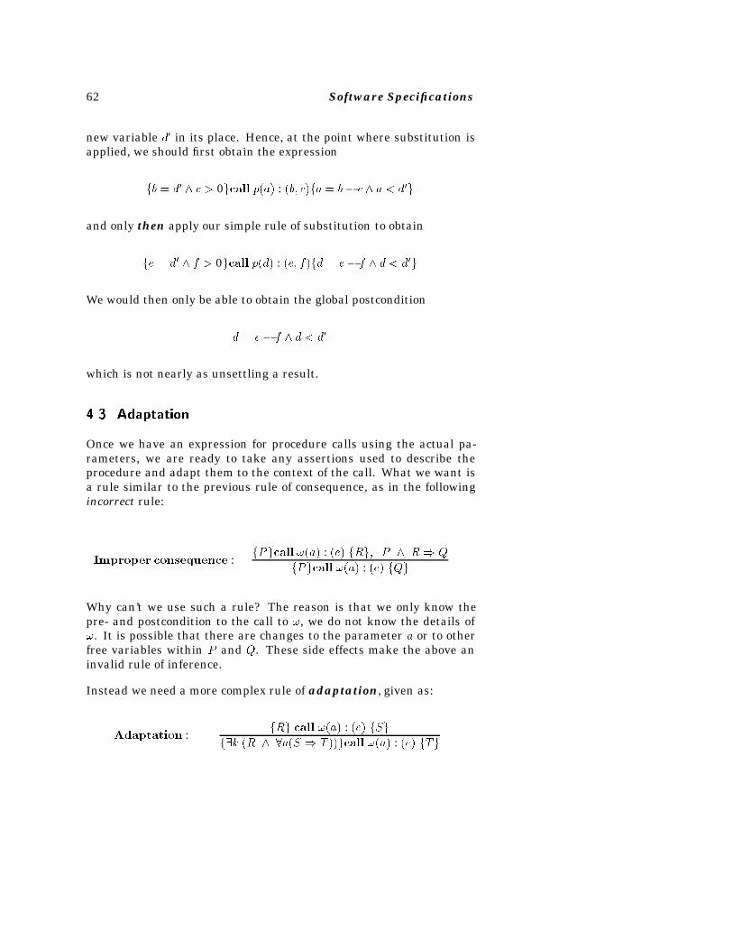
62 Software Specifications
new variable d� in its place. Hence, at the point where substitution isapplied, we should first obtain the expression
fb � d� c � 0gcall p�a� : �b� c�fa � b� c a � d�g
and only then apply our simple rule of substitution to obtain
fe � d� f � 0gcall p�d� : �e� f�fd � e � f d � d�g
We would then only be able to obtain the global postcondition
d � e � f d � d�
which is not nearly as unsettling a result.
���� Adaptation
Once we have an expression for procedure calls using the actual pa-rameters, we are ready to take any assertions used to describe theprocedure and adapt them to the context of the call. What we want isa rule similar to the previous rule of consequence, as in the followingincorrect rule:
Improper consequence :fPgcall �a� : �e� fRg� P R Q
fPgcall �a� : �e� fQg
Why can’t we use such a rule? The reason is that we only know thepre- and postcondition to the call to , we do not know the details of. It is possible that there are changes to the parameter a or to otherfree variables within P and Q. These side effects make the above aninvalid rule of inference.
Instead we need a more complex rule of adaptation, given as:
Adaptation :fRg call �a� : �e� fSg
f�k �R �a�S T ��gcall �a� : �e� fTg
The Axiomatic Approach 63
where k is the list of all variables free in R and S but not occurringin a, e, or T . While the motivation for why this rule appears as itdoes is obscure at first, what we are saying is that there must be someassignment to the free variables of R and S (i.e., k) which makes a trueprecondition R to the call of , such that for any possible alterationwithin to the parameter a, S will still imply T . If so, then we can useour “rule of consequence” above to produce T as a postcondition.
In order to better understand the role of the axioms to represent pro-cedure calls, the following examples are presented.
Universal quanti�cation in adaptation
The following example illustrates the need for universal quantificationof parameters whose values may vary. Consider the following proce-dure p:
p�x� y� : �� procedure � fprecondition x � 3 y � 4postcondition x � y � 12int t;t :� x;x :� y;y :� t;g
Suppose we want to show:
fa � 3 b � 4gcall p�a� b� : ��fa � b � 12 a � bg
After using invocation and substitution, we can conclude:
fa � 3 b � 4gcall p�a� b� : ��fa � b � 12g
Using the improper rule of consequence, we could combine this resultwith a proof of the implication:
�a � 3 b � 4 a � b � 12� �a � b � 12 a � b�
to achieve our goal.
However, using adaptation, the results of invocation and substitutiononly permit us to conclude:
64 Software Specifications
�a � 3 b � 4� ��a� b�a � b � 12� �a � b � 12 a � b��call p�a� b� : ��fa � b � 12 a � bg
Since any quantified variable can be renamed, we could rewrite theconclusion as:
�a � 3 b � 4� ��m�n�m � n � 12� �m � n � 12 m � n��call p�a� b� : ��fa � b � 12 a � bg
Thus, it is clear that assertions about values of variable parametersbefore a call (e.g., a � 3 b � 4) cannot be used to prove assertionsabout their values after the call (e.g., m � n).
Existential quanti�cation in adaptation
Consider the trivial program
fx � x�gx :� x� 1fx � x� � 1g
with the pre- and postconditions as given. We might elect to encapsu-late this fragment into a procedure (call it �x� : ��) and try to provethe program
ftrueg z :� 1; call �z� : ��fz � 2g
After proving the body of the procedure using assignment, we use in-vocation to conclude:
fx � x�gx :� x� 1fx � x� � 1gfx � x�g call �x� : ��fx � x� � 1g
Then using our rule of substitution, we can obtain:
fx � x�g call �x� : ��fx � x� � 1gfz � x�g call �z� : ��fz � x� � 1g
Using an adaptation rule without existentally quantifying x’ we obtain:
The Axiomatic Approach 65
fz � x�g call �z� : ��fz � x� � 1gf�z � x� �z�z � x� � 1 z � 2��g call �z� : ��fz � 2g
Now when we use the assignment axiom, we have:
f1 � x��z�z � x��1 z � 2��gz :� 1f�z � x��z�z � x��1 z � 2��g
or simply:
f1 � x�g z :� 1 f�z � x� �z�z � x� � 1 z � 2��g
Unfortunately, we cannot show (true 1 � x�) so that we can apply arule of consequence to conclude
ftrueg z :� 1 f�z � x� �z�z � x� � 1 z � 2��g
However, had we used the existential quantifier in adaptation, wewould have concluded:
fz � x�g call �z� : ��fz � x� � 1gf�x��z � x� �z�z � x� � 1 z � 2��g call �z� : ��fz � 2g
The result of the adaptation axiom asks whether there is any assign-ment to the free variables of the pre- and postconditions (e.g., 1 in thiscase) such that no matter what happens to z inside , the postconditionwill imply the derived result. If our program’s input assertion impliesthis, then we can always get the derived answer. Or in other words, wewant to be able to prove:
z � 1 �x��z � x� �z�z � x� � 1 z � 2��
But clearly this is the case, since we can satisfy the implication byselecting x� � 1 in the existential quantifier.
Since this last statement is just a logical implication, we can apply ournormal rule of consequence to conclude:
fz � 1g call �z� : ��fz � 2g
Now the assignment axiom yields:
f1 � 1g z :� 1 fz � 1g
and the proof can be completed using composition.
66 Software Specifications
���� Detailed Example� Simple Sums
The following is a detailed example (adapted from [61]) of how ourinference rules for procedure call and parameters can be employed.
PROGRAM � fprocedure e�x� : �y� z� � f
precondition � z � 0 y �� 0postcondition � x � yz
new i;i :� 0;x :� 1;while i � z do
i :� i � 1;x :� xyg
new a� p� s� n;a :� 1;n :� 3;s :� 0;while a � m do
call e�p� : �a� n�;s :� s� p;a :� a� 1g
For this program, the input condition ism � 0 and the output conditionis s �
Pmi�1 i
3.
Procedure body
Proof: We begin by showing that the procedure e satisfies its specifi-cation, that is, fy �� 0 z � 0gbody of efx � yzg. The loop invariant forthe while statement in the procedure body is y �� 0x � yi 0 � i � z.
First, we verify that the invariant holds before execution of the whilestatement. Twice using our axiom of assignment we see that
f1 � yi 0 � i � zgx :� 1fx � yi 0 � i � zgf1 � y0 0 � 0 � zgi :� 0f1 � yi 0 � i � zg
then these can be composed to yield
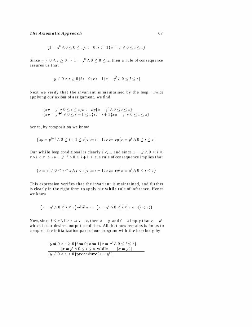
The Axiomatic Approach 67
f1 � y0 0 � 0 � zgi :� 0;x :� 1fx � yi 0 � i � zg
Since y �� 0 z � 0 1 � y0 0 � 0 � z, then a rule of consequenceassures us that
fy �� 0 z � 0gi :� 0;x :� 1fx � yi 0 � i � zg
Next we verify that the invariant is maintained by the loop. Twiceapplying our axiom of assignment, we find:
fxy � yi 0 � i � zgx :� xyfx � yi 0 � i � zgfxy � yi�1 0 � i � 1 � zgi :� i� 1fxy � yi 0 � i � zg
hence, by composition we know
fxy � yi�1 0 � i� 1 � zgi :� i � 1;x :� xyfx � yi 0 � i � zg
Our while loop conditional is clearly i � z, and since x � yi 0 � i �z i � z xy � yi�1 0 � i� 1 � z, a rule of consequence implies that
fx � yi 0 � i � z i � zgi :� i � 1;x :� xyfx � yi 0 � i � zg
This expression verifies that the invariant is maintained, and furtheris clearly in the right form to apply our while rule of inference. Hencewe know
fx � yi 0 � i � zgwhile � � � fx � yi 0 � i � z ��i � z�g
Now, since i � z i � z i � z, then x � yi and i � z imply that x � yz
which is our desired output condition. All that now remains is for us tocompose the initialization part of our program with the loop body, by
fy �� 0 z � 0gi :� 0;x :� 1fx � yi 0 � i � zg�fx � yi 0 � i � zgwhile � � � fx � yzg
fy �� 0 z � 0gprocedurefx � yzg
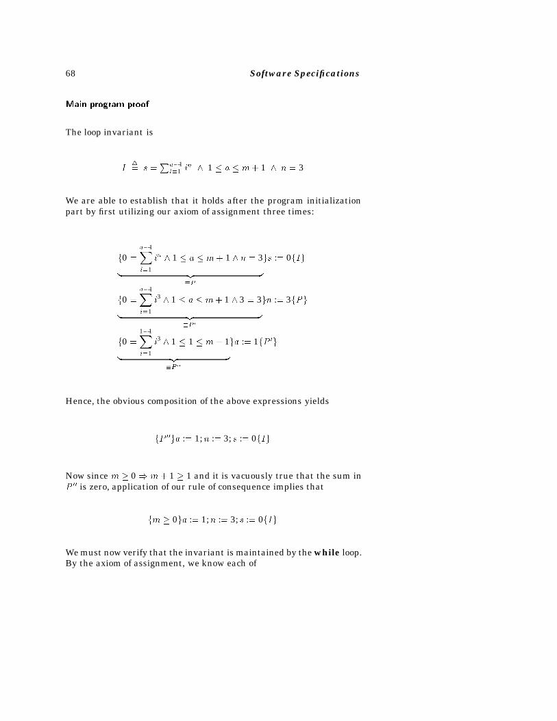
68 Software Specifications
Main program proof
The loop invariant is
I�� s �
Pa�1i�1 i
n 1 � a � m� 1 n � 3
We are able to establish that it holds after the program initializationpart by first utilizing our axiom of assignment three times:
f0 �a�1Xi�1
in 1 � a � m � 1 n � 3
� �z ��P
gs :� 0fIg
f0 �a�1Xi�1
i3 1 � a � m � 1 3 � 3
� �z ��P �
gn :� 3fPg
f0 �1�1Xi�1
i3 1 � 1 � m � 1
� �z ��P ��
ga :� 1fP �g
Hence, the obvious composition of the above expressions yields
fP ��ga :� 1;n :� 3; s :� 0fIg
Now since m � 0 m � 1 � 1 and it is vacuously true that the sum inP �� is zero, application of our rule of consequence implies that
fm � 0ga :� 1;n :� 3; s :� 0fIg
We must now verify that the invariant is maintained by the while loop.By the axiom of assignment, we know each of
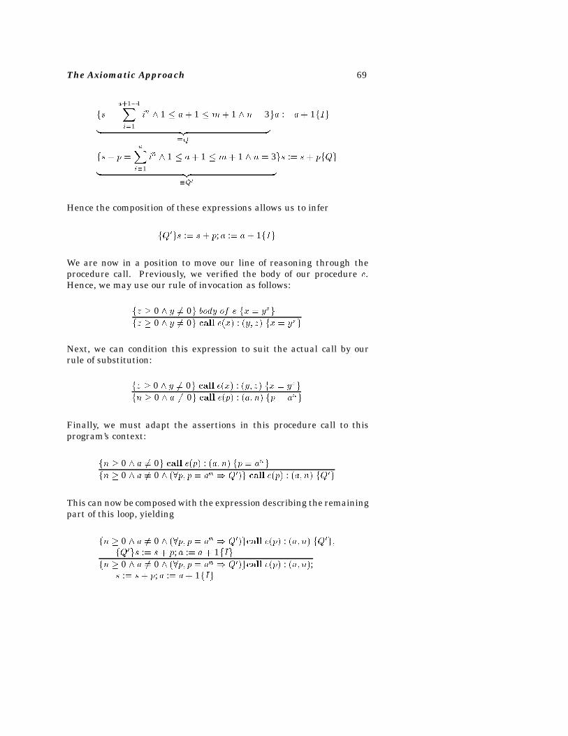
The Axiomatic Approach 69
fs �a�1�1Xi�1
in 1 � a� 1 � m � 1 n � 3
� �z ��Q
ga :� a� 1fIg
fs� p �aXi�1
in 1 � a� 1 � m� 1 n � 3
� �z ��Q�
gs :� s � pfQg
Hence the composition of these expressions allows us to infer
fQ�gs :� s � p; a :� a � 1fIg
We are now in a position to move our line of reasoning through theprocedure call. Previously, we verified the body of our procedure e.Hence, we may use our rule of invocation as follows:
fz � 0 y �� 0g body of e fx � yzg
fz � 0 y �� 0g call e�x� : �y� z� fx � yzg
Next, we can condition this expression to suit the actual call by ourrule of substitution:
fz � 0 y �� 0g call e�x� : �y� z� fx � yzgfn � 0 a �� 0g call e�p� : �a� n� fp � ang
Finally, we must adapt the assertions in this procedure call to thisprogram’s context:
fn � 0 a �� 0g call e�p� : �a� n� fp � ang
fn � 0 a �� 0 ��p� p � an Q��g call e�p� : �a� n� fQ�g
This can now be composed with the expression describing the remainingpart of this loop, yielding
fn � 0 a �� 0 ��p� p � an Q��gcall e�p� : �a� n� fQ�g�fQ�gs :� s� p; a :� a� 1fIg
fn � 0 a �� 0 ��p� p � an Q��gcall e�p� : �a� n�;s :� s� p; a :� a� 1fIg
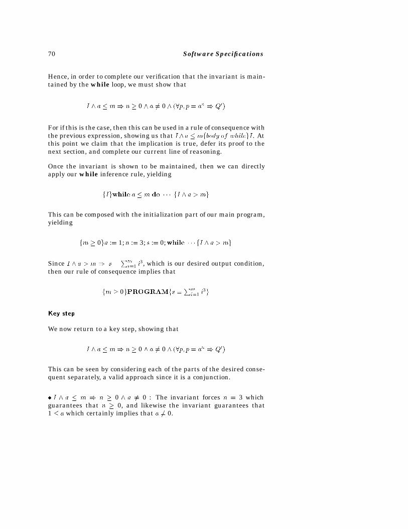
70 Software Specifications
Hence, in order to complete our verification that the invariant is main-tained by the while loop, we must show that
I a � m n � 0 a �� 0 ��p� p � an Q��
For if this is the case, then this can be used in a rule of consequence withthe previous expression, showing us that I a � mfbody of whilegI. Atthis point we claim that the implication is true, defer its proof to thenext section, and complete our current line of reasoning.
Once the invariant is shown to be maintained, then we can directlyapply our while inference rule, yielding
fIgwhile a � m do � � � fI a � mg
This can be composed with the initialization part of our main program,yielding
fm � 0ga :� 1;n :� 3; s :� 0;while � � � fI a � mg
Since I a � m s �Pm
i�1 i3, which is our desired output condition,
then our rule of consequence implies that
fm � 0gPROGRAMfs �Pm
i�1 i3g
Key step
We now return to a key step, showing that
I a � m n � 0 a �� 0 ��p� p � an Q��
This can be seen by considering each of the parts of the desired conse-quent separately, a valid approach since it is a conjunction.
� I a � m n � 0 a �� 0 : The invariant forces n � 3 whichguarantees that n � 0, and likewise the invariant guarantees that1 � a which certainly implies that a �� 0.
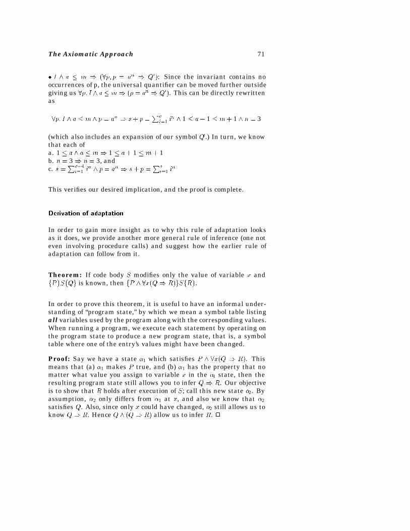
The Axiomatic Approach 71
� I a � m ��p� p � an Q��: Since the invariant contains nooccurrences of p, the universal quantifier can be moved further outsidegiving us �p� I a � m �p � an Q��. This can be directly rewrittenas
�p� I a � m p � an s� p �Pa
i�1 in 1 � a� 1 � m� 1 n � 3
(which also includes an expansion of our symbol Q�.) In turn, we knowthat each ofa. 1 � a a � m 1 � a� 1 � m � 1b. n � 3 n � 3, andc. s �
Pa�1i�1 i
n p � an s � p �Pa
i�1 in
This verifies our desired implication, and the proof is complete.
Derivation of adaptation
In order to gain more insight as to why this rule of adaptation looksas it does, we provide another more general rule of inference (one noteven involving procedure calls) and suggest how the earlier rule ofadaptation can follow from it.
Theorem: If code body S modifies only the value of variable x andfPgSfQg is known, then fP �x�Q R�gSfRg.
In order to prove this theorem, it is useful to have an informal under-standing of “program state,” by which we mean a symbol table listingall variables used by the program along with the corresponding values.When running a program, we execute each statement by operating onthe program state to produce a new program state, that is, a symboltable where one of the entry’s values might have been changed.
Proof: Say we have a state �1 which satisfies P �x�Q R�. Thismeans that (a) �1 makes P true, and (b) �1 has the property that nomatter what value you assign to variable x in the �1 state, then theresulting program state still allows you to infer Q R. Our objectiveis to show that R holds after execution of S; call this new state �2. Byassumption, �2 only differs from �1 at x, and also we know that �2satisfies Q. Also, since only x could have changed, �2 still allows us toknow Q R. Hence Q �Q R� allow us to infer R. �
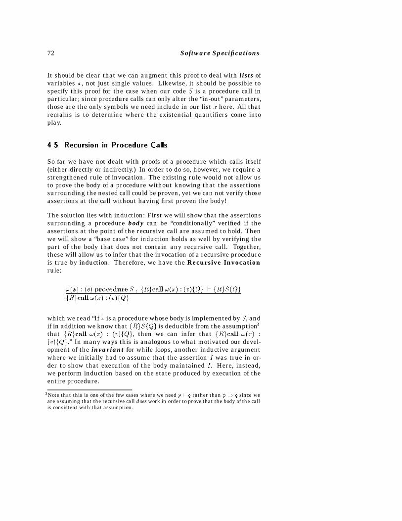
72 Software Specifications
It should be clear that we can augment this proof to deal with lists ofvariables x, not just single values. Likewise, it should be possible tospecify this proof for the case when our code S is a procedure call inparticular; since procedure calls can only alter the “in-out” parameters,those are the only symbols we need include in our list x here. All thatremains is to determine where the existential quantifiers come intoplay.
���� Recursion in Procedure Calls
So far we have not dealt with proofs of a procedure which calls itself(either directly or indirectly.) In order to do so, however, we require astrengthened rule of invocation. The existing rule would not allow usto prove the body of a procedure without knowing that the assertionssurrounding the nested call could be proven, yet we can not verify thoseassertions at the call without having first proven the body!
The solution lies with induction: First we will show that the assertionssurrounding a procedure body can be “conditionally” verified if theassertions at the point of the recursive call are assumed to hold. Thenwe will show a “base case” for induction holds as well by verifying thepart of the body that does not contain any recursive call. Together,these will allow us to infer that the invocation of a recursive procedureis true by induction. Therefore, we have the Recursive Invocationrule:
�x� : �v� procedure S � fRgcall �x� : �v�fQg � fRgSfQg
fRgcall �x� : �v�fQg
which we read “If is a procedure whose body is implemented by S, andif in addition we know that fRgSfQg is deducible from the assumption3
that fRgcall �x� : �v�fQg, then we can infer that fRgcall �x� :�v�fQg.” In many ways this is analogous to what motivated our devel-opment of the invariant for while loops, another inductive argumentwhere we initially had to assume that the assertion I was true in or-der to show that execution of the body maintained I. Here, instead,we perform induction based on the state produced by execution of theentire procedure.
3Note that this is one of the few cases where we need p � q rather than p � q since weare assuming that the recursive call does work in order to prove that the body of the callis consistent with that assumption.
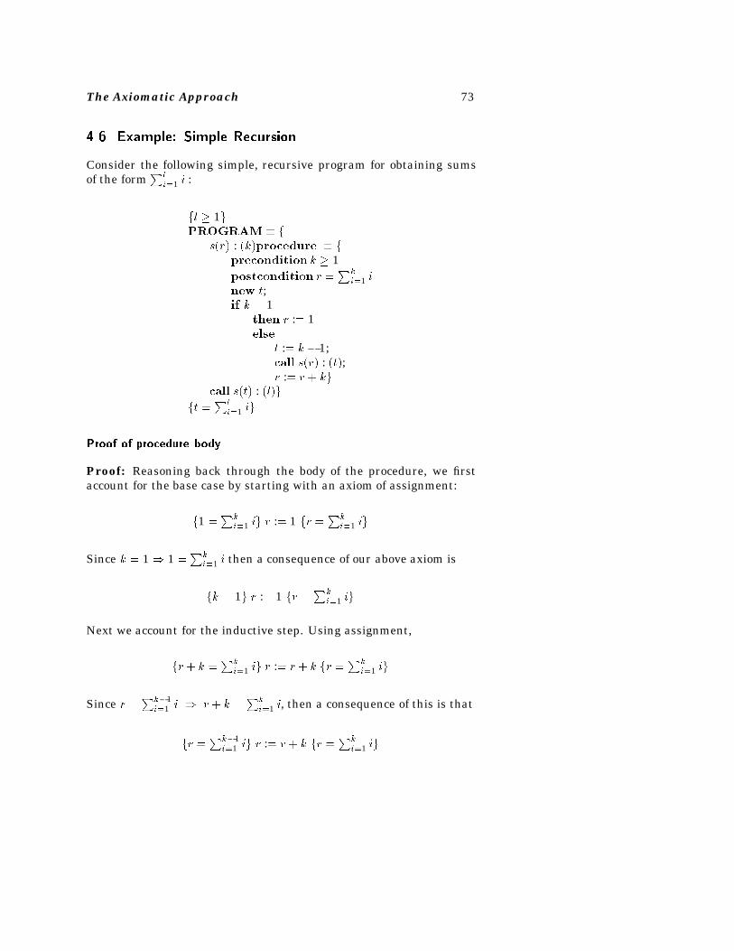
The Axiomatic Approach 73
���� Example� Simple Recursion
Consider the following simple, recursive program for obtaining sumsof the form
Pli�1 i :
fl � 1gPROGRAM � f
s�r� : �k�procedure � fprecondition k � 1postcondition r �
Pki�1 i
new t;if k � 1
then r :� 1else
t :� k � 1;call s�r� : �t�;r :� r � kg
call s�t� : �l�gft �
Pli�1 ig
Proof of procedure body
Proof: Reasoning back through the body of the procedure, we firstaccount for the base case by starting with an axiom of assignment:
f1 �Pk
i�1 ig r :� 1 fr �Pk
i�1 ig
Since k � 1 1 �Pk
i�1 i then a consequence of our above axiom is
fk � 1g r :� 1 fr �Pk
i�1 ig
Next we account for the inductive step. Using assignment,
fr � k �Pk
i�1 ig r :� r � k fr �Pk
i�1 ig
Since r �Pk�1
i�1 i r � k �Pk
i�1 i, then a consequence of this is that
fr �Pk�1
i�1 ig r :� r � k fr �Pk
i�1 ig
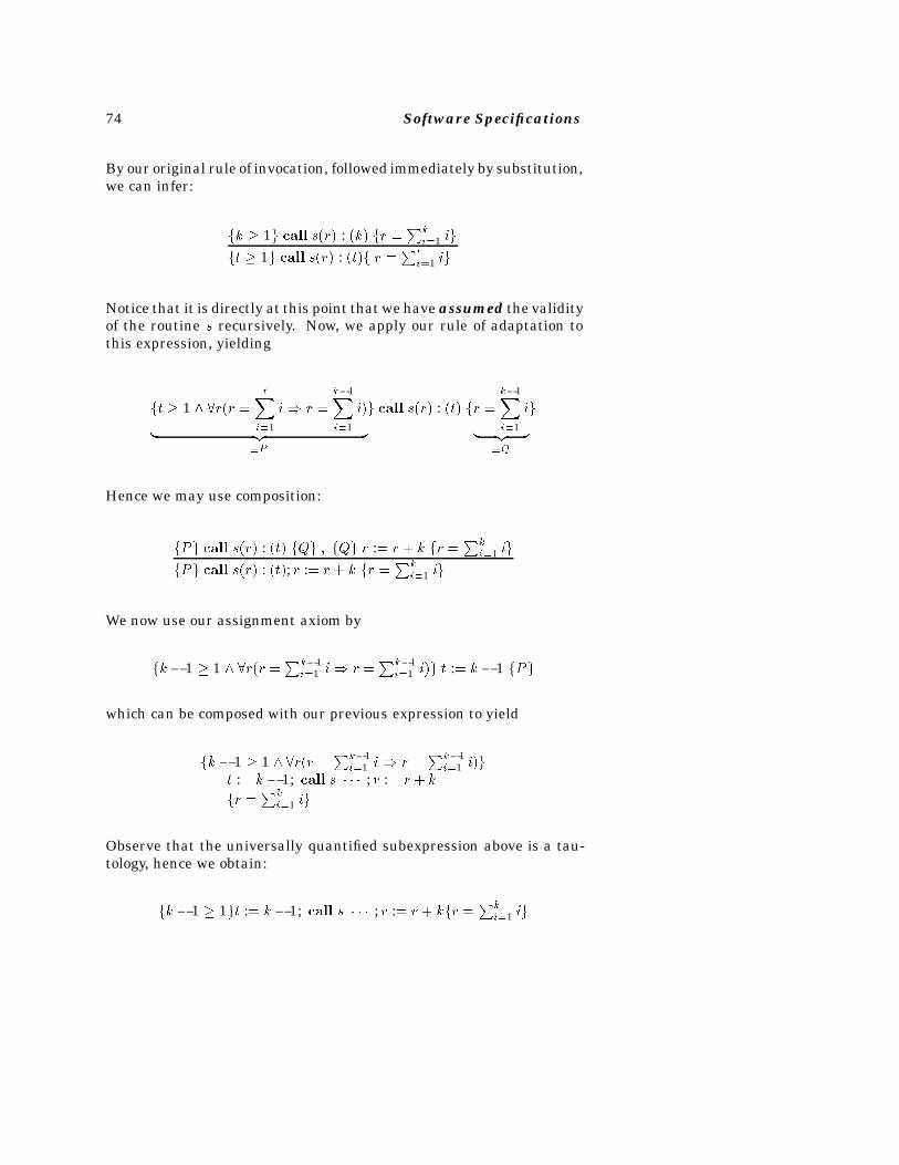
74 Software Specifications
By our original rule of invocation, followed immediately by substitution,we can infer:
fk � 1g call s�r� : �k� fr �Pk
i�1 ig
ft � 1g call s�r� : �t�f r �Pt
i�1 ig
Notice that it is directly at this point that we have assumed the validityof the routine s recursively. Now, we apply our rule of adaptation tothis expression, yielding
ft � 1 �r�r �tX
i�1
i r �k�1Xi�1
i�
� �z ��P
g call s�r� : �t� fr �k�1Xi�1
i
� �z ��Q
g
Hence we may use composition:
fPg call s�r� : �t� fQg � fQg r :� r � k fr �Pk
i�1 ig
fPg call s�r� : �t�; r :� r � k fr �Pk
i�1 ig
We now use our assignment axiom by
fk� 1 � 1 �r�r �Pk�1
i�1 i r �Pk�1
i�1 i�g t :� k � 1 fPg
which can be composed with our previous expression to yield
fk � 1 � 1 �r�r �Pk�1
i�1 i r �Pk�1
i�1 i�gt :� k � 1; call s � � � ; r :� r � k
fr �Pk
i�1 ig
Observe that the universally quantified subexpression above is a tau-tology, hence we obtain:
fk � 1 � 1gt :� k � 1; call s � � � ; r :� r � kfr �Pk
i�1 ig
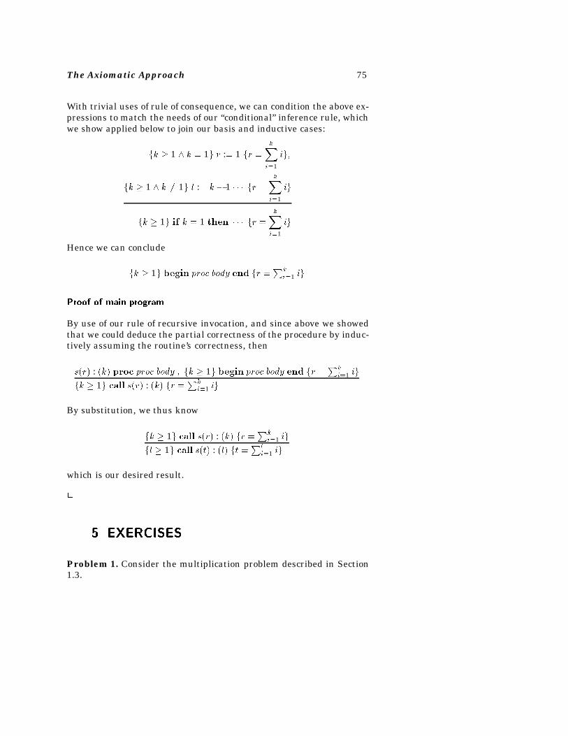
The Axiomatic Approach 75
With trivial uses of rule of consequence, we can condition the above ex-pressions to match the needs of our “conditional” inference rule, whichwe show applied below to join our basis and inductive cases:
fk � 1 k � 1g r :� 1 fr �kXi�1
ig�
fk � 1 k �� 1g t :� k � 1 � � � fr �kXi�1
ig
fk � 1g if k � 1 then � � � fr �kXi�1
ig
Hence we can conclude
fk � 1g begin proc body end fr �Pk
i�1 ig
Proof of main program
By use of our rule of recursive invocation, and since above we showedthat we could deduce the partial correctness of the procedure by induc-tively assuming the routine’s correctness, then
s�r� : �k� proc proc body � fk � 1g begin proc body end fr �Pk
i�1 ig
fk � 1g call s�r� : �k� fr �Pk
i�1 ig
By substitution, we thus know
fk � 1g call s�r� : �k� fr �Pk
i�1 ig
fl � 1g call s�t� : �l� ft �Pl
i�1 ig
which is our desired result.
�
�� EXERCISES
Problem 1. Consider the multiplication problem described in Section1.3.
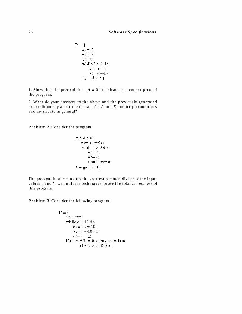
76 Software Specifications
P � fa :� A;b :� B;y :� 0;while b � 0 do
y :� y � ab :� b� 1g
fy � A�Bg
1. Show that the precondition fA � 0g also leads to a correct proof ofthe program.
2. What do your answers to the above and the previously generatedprecondition say about the domain for A and B and for preconditionsand invariants in general?
Problem 2. Consider the program
fa � b � 0gr :� a mod b;while r � 0 do
a :� b;b :� r;r :� a mod b;
fb � gcd��a �
�
b �g
The postcondition means b is the greatest common divisor of the inputvalues a and b. Using Hoare techniques, prove the total correctness ofthis program.
Problem 3. Consider the following program:
P � fs :� sum;while s � 10 do
x :� s div 10;y :� s � 10 � x;s :� x� y;
if �s mod 3� � 0 then ans :� true
else ans :� false g
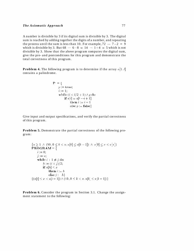
The Axiomatic Approach 77
A number is divisible by 3 if its digital sum is divisible by 3. The digitalsum is reached by adding together the digits of a number, and repeatingthe process until the sum is less than 10. For example, 72 � 7�2 � 9which is divisible by 3. But 68 � 6�8 � 14 � 1�4 � 5 which is notdivisible by 3. Show that the above program computes the digital sum,give the pre- and postconditions for this program and demonstrate thetotal correctness of this program.
Problem 4. The following program is to determine if the array a�1��l�contains a palindrome.
P � fp :� true;i :� 1;while �i � l2 � 1� p do
if a�i� � a�l � i� 1�then i :� i� 1else p :� falseg
Give input and output specifications, and verify the partial correctnessof this program.
Problem 5. Demonstrate the partial correctness of the following pro-gram:
fn � 1 ��k� 0 � k � n� a�k� � a�k � 1�� a�0� � x � a�n�gPROGRAM � f
i :� 0;j :� n;while i� 1 �� j do
h :� �i� j�2;if a�h� � x
then i :� helse j :� hg
f�a�i� � x � a�i� 1�� ��k� 0 � k � n� a�k� � a�k� 1��g
Problem 6. Consider the program in Section 3.1. Change the assign-ment statement to the following:
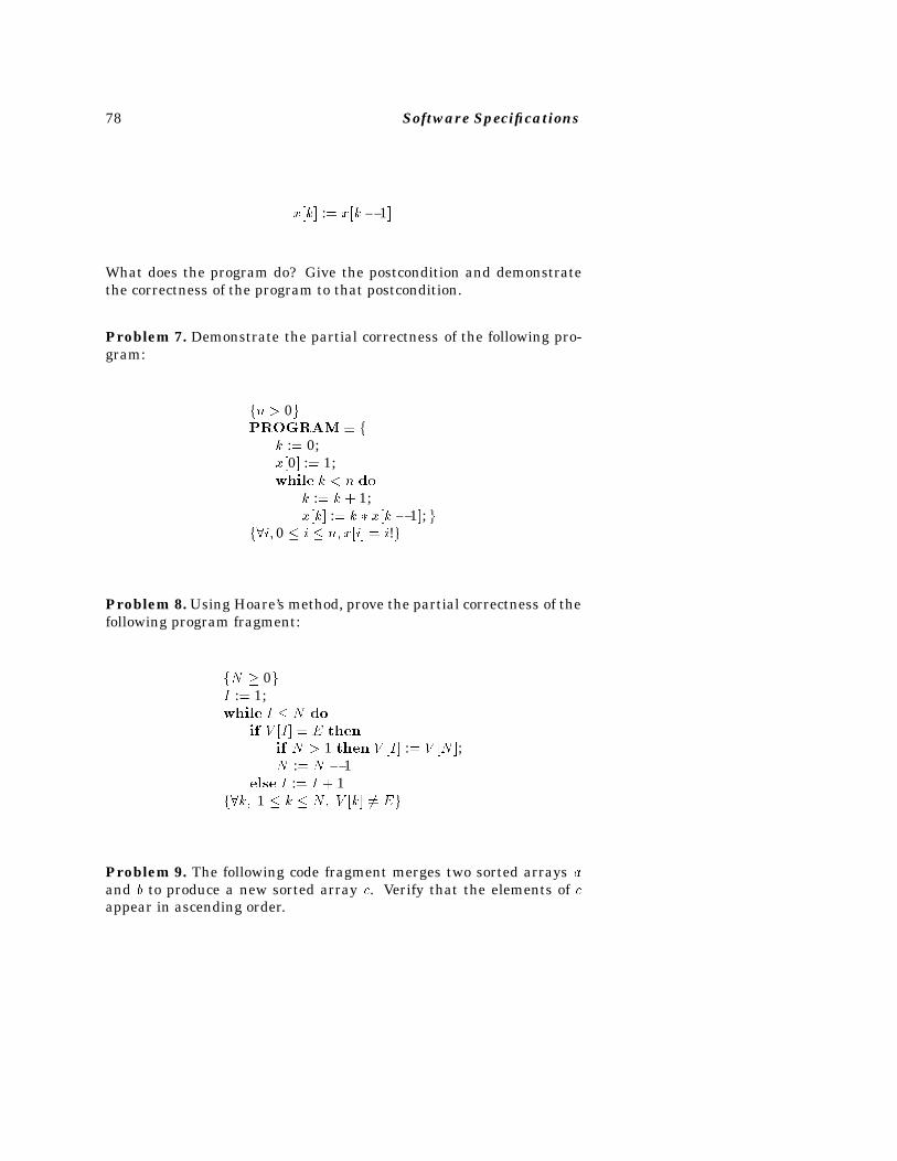
78 Software Specifications
x�k� :� x�k� 1�
What does the program do? Give the postcondition and demonstratethe correctness of the program to that postcondition.
Problem 7. Demonstrate the partial correctness of the following pro-gram:
fn � 0gPROGRAM � f
k :� 0;x�0� :� 1;while k � n do
k :� k � 1;x�k� :� k � x�k � 1�; g
f�i� 0 � i � n� x�i� � i!g
Problem 8. Using Hoare’s method, prove the partial correctness of thefollowing program fragment:
fN � 0gI :� 1;while I � N do
if V �I� � E then
if N � 1 then V �I� :� V �N �;N :� N � 1
else I :� I � 1f�k� 1 � k � N� V �k� �� Eg
Problem 9. The following code fragment merges two sorted arrays aand b to produce a new sorted array c. Verify that the elements of cappear in ascending order.
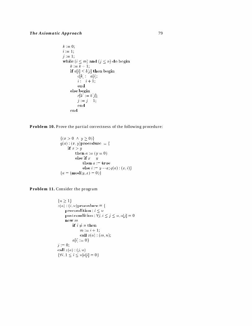
The Axiomatic Approach 79
k :� 0;i :� 1;j :� 1;while �i � m� and �j � n� do begin
k :� k � 1;if a�i� � b�j� then begin
c�k� :� a�i�;i :� i� 1;end
else begin
c�k� :� b�j�;j :� j � 1;end
end
Problem 10. Prove the partial correctness of the following procedure:
f�x � 0 y � 0�gq�a� : �x� y�procedure � f
if x � ythen a :� �y � 0�else if x � y
then a :� true
else i :� y � x; q�a� : �x� i�gfa � �mod�y� x� � 0�g
Problem 11. Consider the program
fn � 1gz�a� : �i� n�procedure� f
precondition : i � npostcondition : �j� i � j � n� a�j� � 0new m
if i �� n thenm :� i� 1;call z�a� : �m�n�;
a�i� :� 0gj :� 0;call z�a� : �j� n�f�i� 1 � i � nja�i� � 0g
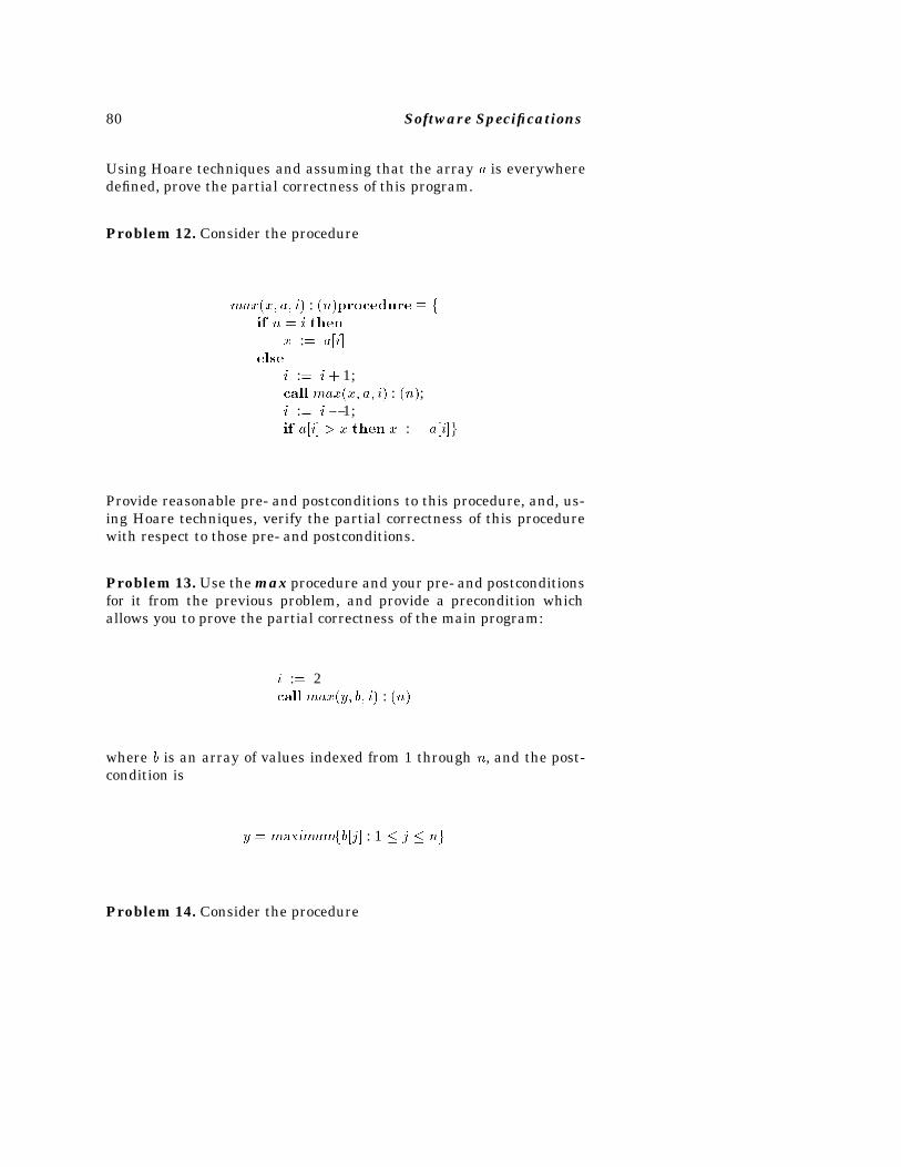
80 Software Specifications
Using Hoare techniques and assuming that the array a is everywheredefined, prove the partial correctness of this program.
Problem 12. Consider the procedure
max�x� a� i� : �n�procedure � fif n � i then
x :� a�i�else
i :� i � 1;call max�x� a� i� : �n�;i :� i � 1;if a�i� � x then x :� a�i�g
Provide reasonable pre- and postconditions to this procedure, and, us-ing Hoare techniques, verify the partial correctness of this procedurewith respect to those pre- and postconditions.
Problem 13. Use the max procedure and your pre- and postconditionsfor it from the previous problem, and provide a precondition whichallows you to prove the partial correctness of the main program:
i :� 2callmax�y� b� i� : �n�
where b is an array of values indexed from 1 through n, and the post-condition is
y � maximumfb�j� : 1 � j � ng
Problem 14. Consider the procedure
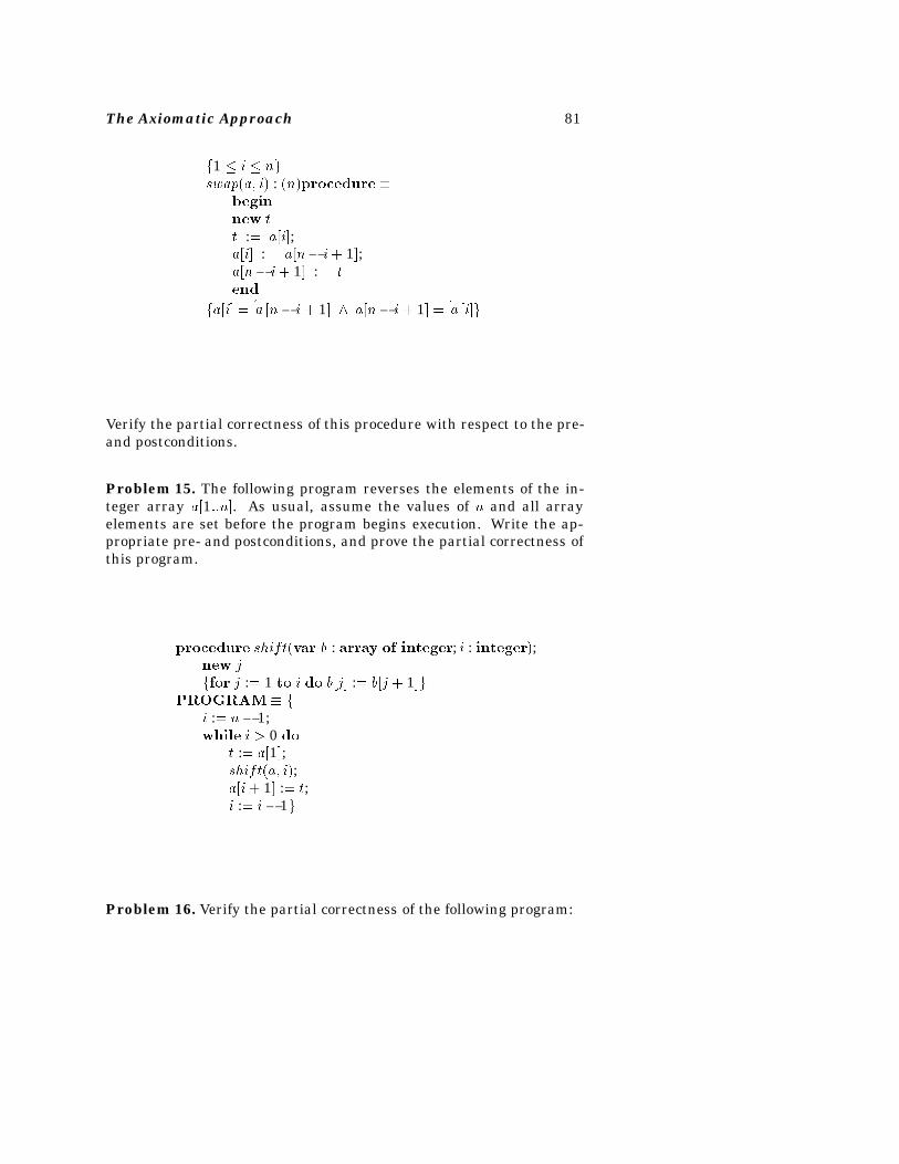
The Axiomatic Approach 81
f1 � i � ngswap�a� i� : �n�procedure �
begin
new tt :� a�i�;a�i� :� a�n� i� 1�;a�n� i� 1� :� tend
fa�i� ��a �n� i � 1� a�n� i � 1� �
�a �i�g
Verify the partial correctness of this procedure with respect to the pre-and postconditions.
Problem 15. The following program reverses the elements of the in-teger array a�1��n�. As usual, assume the values of n and all arrayelements are set before the program begins execution. Write the ap-propriate pre- and postconditions, and prove the partial correctness ofthis program.
procedure shift�var b : array of integer; i : integer�;new jffor j :� 1 to i do b�j� :� b�j � 1�g
PROGRAM � fi :� n� 1;while i � 0 do
t :� a�1�;shift�a� i�;a�i� 1� :� t;i :� i � 1g
Problem 16. Verify the partial correctness of the following program:
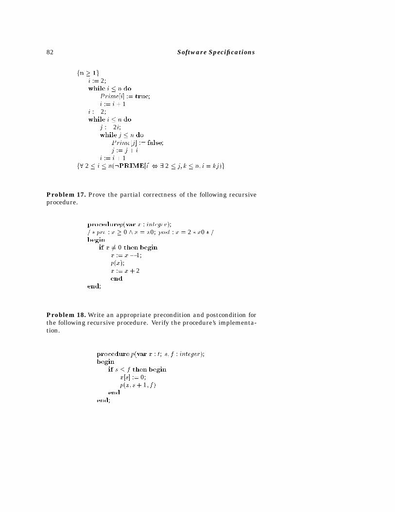
82 Software Specifications
fn � �gi :� 2;while i � n do
Prime�i� :� true;i :� i � 1
i :� 2;while i � n do
j :� 2i;while j � n do
Prime�j� :� false;j :� j � i
i :� i � 1f� 2 � i � n��PRIME�i�� � 2 � j� k � n� i � kj�g
Problem 17. Prove the partial correctness of the following recursiveprocedure.
procedurep�var x : integer�; � pre : x � 0 x � x0; post : x � 2 � x0 � begin
if x �� 0 then beginx :� x� 1;p�x�;x :� x� 2end
end;
Problem 18. Write an appropriate precondition and postcondition forthe following recursive procedure. Verify the procedure’s implementa-tion.
procedure p�var x : t; s� f : integer�;begin
if s � f then beginx�s� :� 0;p�x� s� 1� f�
end
end;
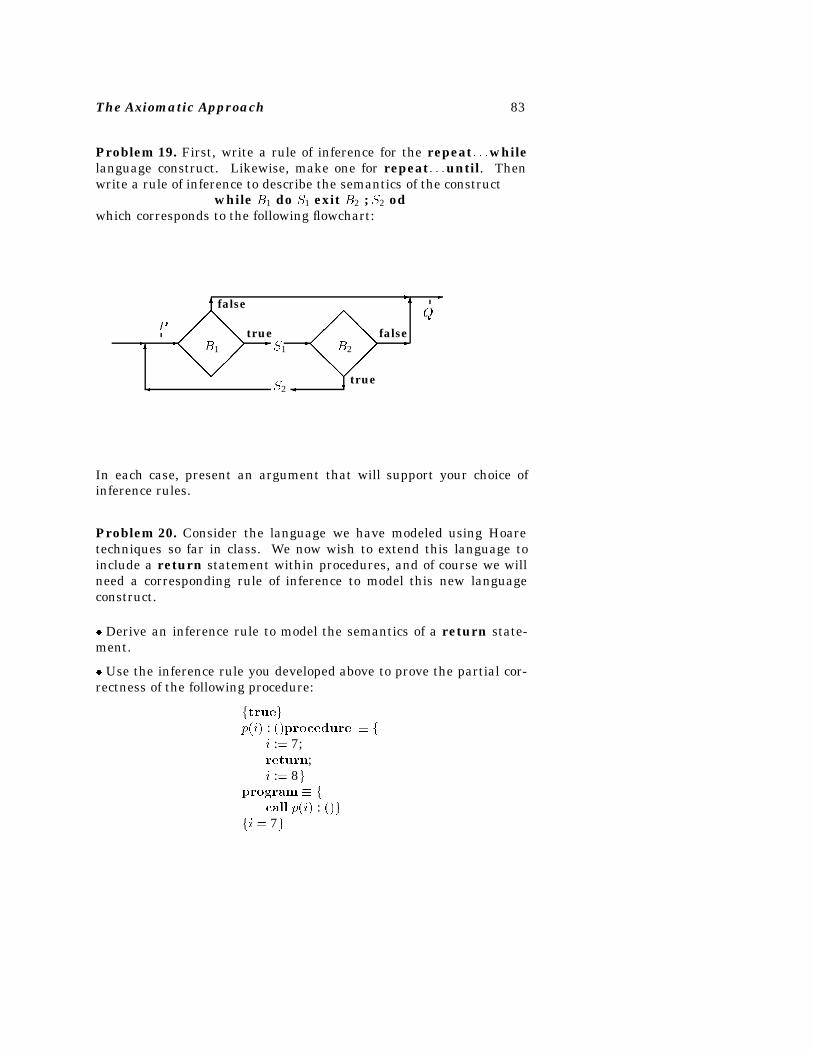
The Axiomatic Approach 83
Problem 19. First, write a rule of inference for the repeat� � �whilelanguage construct. Likewise, make one for repeat� � �until. Thenwrite a rule of inference to describe the semantics of the construct
while B1 do S1 exit B2 ; S2 odwhich corresponds to the following flowchart:
���
���
���
���
B1
���
���
���
���
B2� � �
S1� �
��
�
�
�� S2
� �
PQ
false
true
true
false
In each case, present an argument that will support your choice ofinference rules.
Problem 20. Consider the language we have modeled using Hoaretechniques so far in class. We now wish to extend this language toinclude a return statement within procedures, and of course we willneed a corresponding rule of inference to model this new languageconstruct.
� Derive an inference rule to model the semantics of a return state-ment.
� Use the inference rule you developed above to prove the partial cor-rectness of the following procedure:
ftruegp�i� : ��procedure � f
i :� 7;return;i :� 8g
program � fcall p�i� : ��g
fi � 7g
84 Software Specifications
�� SUGGESTED READINGS
The original work on this axiomatic approach is due to Floyd and Hoare,and entries in the following list ought to be viewed as “classics.”
� R.W. Floyd, “Assigning Meanings to Programs,” Symposium in Ap-plied Mathematics 19, American Mathematical Society, 1967, pp. 19-32.
� C.A.R. Hoare, “An Axiomatic Basic for Computer Programming,”Communications of the ACM, Vol. 12, No. 10, October, 1969, pp. 576-580, 583.
� C.A.R. Hoare, “Procedures and Parameters, An Axiomatic Approach,”Symposium on the Semantics of Algorithmic Languages, Springer-Verlag, New York, 1971, pp. 102-116.
� C.A.R. Hoare and N. Wirth, “An Axiomatic Definition of the Program-ming Language PASCAL,” Acta Informatica, Vol. 2, 1973, pp. 335-355.
� D.C. Luckham and N. Suzuki, “Verification of Array, Record, andPointer Operations in Pascal,” ACM Transactions on ProgrammingLanguages and Systems, Vol. 1, No. 2, October, 1979, pp. 226-244.
Readers will find these classics nicely augmented by these works:
� J.H. Remmers, “A Technique for Developing Loop Invariants,” Infor-mation Processing Letters, Vol. 18, 1984, pp. 137-139.
� J.C. Reynolds, The Craft of Computer Programming, Prentice-Hall,Englewood Cliffs, NJ, 1981.
Examples of more recent work that are related to the original work ofFloyd and Hoare (either applying it or extending it) are found in:
� L. Lamport and F.B. Schneider, “The ‘Hoare Logic’ of CSP, and AllThat,” ACM Transactions on Programming Languages and Systems,Vol. 6, No. 2, April 1984, pp. 281-296.
� D. Gries and G. Levin, “Assignment and Procedure Call Proof Rules,”ACM Transactions on Programming Languages and Systems, Vol. 2,No. 4, October 1980, pp. 564-579.
Functional Correctness*
Chapter 3
.
Let � be a string representing a source program. For example, a Pascalprogram is just the linear string:
PROGRAM main�input� output�; � � �END�
We express the mathematical function denoted by program � by a boxnotation. � represents the function that computes the same values asprogram �.
Although a function is the intuitive model of a specification, often wesimply want one feasible solution out of many possibilities. For exam-ple, by choosing one optimal strategy among several equivalent ones(e.g., equivalent optimal moves in a game-playing program), we usuallydo not care which solution the program employs. Because of this, weonly need to define a specification as a relation. If r is such a specifica-tion relation, it is equivalent to a program p by the following correctnesstheorem:
Theorem:Program p is correct with respect to specification relation rif and only if domain�r � p � � domain�r�.
�Parts of this chapter are a revision of an earlier paper [64]. Copyright c�1993 by Aca-demic Press, Inc. Reprinted by permission of Academic Press.
85
86 Software Specifications
In other words, if we take the subset of r by considering those pairs inr that are also in function p (i.e., r � p ) we have a function. If thisfunction has the same domain as r, then p includes a pair of values foreach member of relation r and we get a feasible (or correct) implemen-tation of the specification. In what follows, however, we will use thesimpler case, where we have chosen the more restricted specificationfunction f instead of the more general relation rwith the correspondingcorrectness theorem of f � p .
�� PROGRAM SEMANTICS
A program is a sequence of declarations followed by a sequence ofstatements. Every program maps a set of values for every variableinto a new set of values. We pattern the following development ontechniques also used in denotational semantics (which we will discussin greater detail in Chapter6). We can define the meaning of such aprogram as follows.
id.Id is a primitive set of objects we will call the variables or identifiersin a program.
value.V alue is a primitive set of values that each member of id cantake. We will assume that value is the set of integers for most of thisdiscussion, but it can be any discrete set of values.
state.The primitive storage mechanism is the state. If id is a set ofvariable names and value is a set of values, a state is a function withthe signature state : id � value. For every member of set id, weassociate a value in value.
Since a state is a function, it is a set of ordered pairs. Thus for state swe can discuss �a� b� � s, or s : id� value and s�a� � b.
Given state s, if a is a variable in a program, we define a �s� as s�a�.
This concept of a state represents the formal model for program storage(e.g., activation records).
expressions.If expr is an expression, expr is the function that ac-cesses the current state function and evaluates the expression (i.e.,“returns its value”). More formally, we state that expr : state � value.
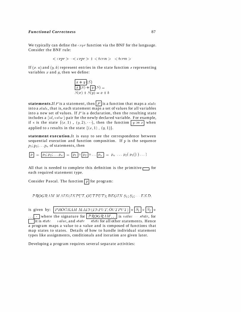
Functional Correctness 87
We typically can define the expr function via the BNF for the language.Consider the BNF rule:
� expr ��� expr � � � term � j � term �
If �x� a� and �y� b� represent entries in the state function s representingvariables x and y, then we define:
x� y �S� �
x �S� � y �S� �
S�x� � S�y� � a� b
statements.IfP is a statement, then P is a function that maps a stateinto a state, that is, each statement maps a set of values for all variablesinto a new set of values. If P is a declaration, then the resulting stateincludes a �id� value� pair for the newly declared variable. For example,if s is the state f�x� 1� � �y� 2�� � � �g, then the function y :� x whenapplied to s results in the state f�x� 1� � �y� 1�g.
statement execution.It is easy to see the correspondence betweensequential execution and function composition. If p is the sequencep1; p2; � � �pn of statements, then
p � p1; p2; � � � pn � p1 p2 � � � pn � pn � � � p2� p1�� � � � � �
All that is needed to complete this definition is the primitive foreach required statement type.
Consider Pascal. The function p for program:
PROGRAM MAIN �INPUT�OUTPUT �;BEGIN S1;S2; � � �END�
is given by: PROGRAM MAIN �INPUT�OUTPUT � S1 S2
� � � � where the signature for PROGRAM � � � is value � state, for� it is state� value, and state� state for all other statements. Hence
a program maps a value to a value and is composed of functions thatmap states to states. Details of how to handle individual statementtypes like assignments, conditionals and iteration are given later.
Developing a program requires several separate activities:
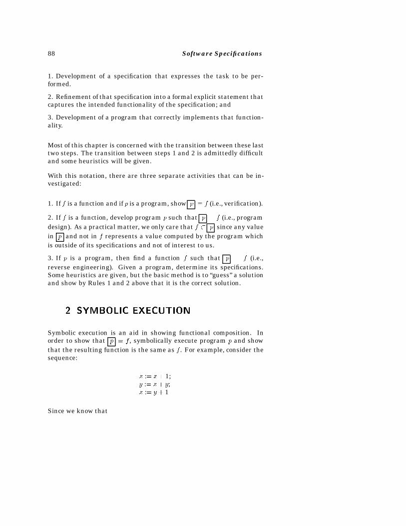
88 Software Specifications
1. Development of a specification that expresses the task to be per-formed.
2. Refinement of that specification into a formal explicit statement thatcaptures the intended functionality of the specification; and
3. Development of a program that correctly implements that function-ality.
Most of this chapter is concerned with the transition between these lasttwo steps. The transition between steps 1 and 2 is admittedly difficultand some heuristics will be given.
With this notation, there are three separate activities that can be in-vestigated:
1. If f is a function and if p is a program, show p � f (i.e., verification).
2. If f is a function, develop program p such that p � f (i.e., programdesign). As a practical matter, we only care that f � p since any valuein p and not in f represents a value computed by the program whichis outside of its specifications and not of interest to us.
3. If p is a program, then find a function f such that p � f (i.e.,reverse engineering). Given a program, determine its specifications.Some heuristics are given, but the basic method is to “guess” a solutionand show by Rules 1 and 2 above that it is the correct solution.
�� SYMBOLIC EXECUTION
Symbolic execution is an aid in showing functional composition. Inorder to show that p � f , symbolically execute program p and showthat the resulting function is the same as f . For example, consider thesequence:
x :� x� 1;y :� x� y;x :� y � 1
Since we know that
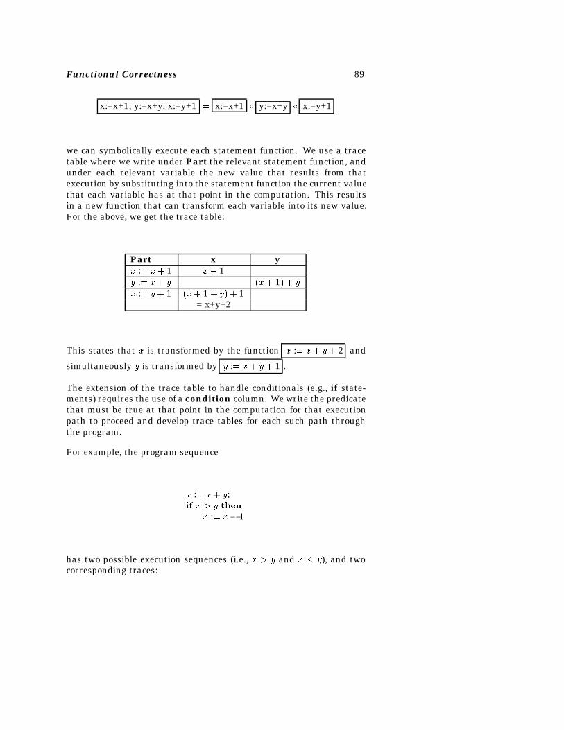
Functional Correctness 89
x:=x+1; y:=x+y; x:=y+1 � x:=x+1 y:=x+y x:=y+1
we can symbolically execute each statement function. We use a tracetable where we write under Part the relevant statement function, andunder each relevant variable the new value that results from thatexecution by substituting into the statement function the current valuethat each variable has at that point in the computation. This resultsin a new function that can transform each variable into its new value.For the above, we get the trace table:
Part x yx :� x� 1 x� 1y :� x� y �x� 1� � yx :� y � 1 �x� 1 � y� � 1
= x+y+2
This states that x is transformed by the function x :� x� y � 2 and
simultaneously y is transformed by y :� x� y � 1 .
The extension of the trace table to handle conditionals (e.g., if state-ments) requires the use of a condition column. We write the predicatethat must be true at that point in the computation for that executionpath to proceed and develop trace tables for each such path throughthe program.
For example, the program sequence
x :� x� y;if x � y then
x :� x� 1
has two possible execution sequences (i.e., x � y and x � y), and twocorresponding traces:
90 Software Specifications
Part Condition x yx :� x� y x� y
if x � y �x� y� � yx :� x� 1 �x� y� � 1
and
Part Condition x yx :� x� y x� y
if x � y �x� y� � y
We summarize these two tables by saying that the function they repre-sent is: “if x�y � y, then the function is x :� x� y � 1 and if x�y � y
then the function is x :� x� y .” In the next section we show how towrite this as a conditional assignment function.
�� DESIGN RULES
As given earlier, software development consists of (a) specification de-sign; (b) formalizing the specification; and (c) developing the sourceprogram. We use a functional notation for (b) that is closely tied tothe eventual source program. This notation includes (a) concurrentassignment; (b) conditional assignment; and (c) loop verification. Thisnotation was strongly influenced by the earlier work by McCarthy onLISP.
���� Design of Assignment Statements
Concurrent assignment is defined as simultaneous assignment. Thefunction: �x� y� z :� y� z� x� simultaneously accesses the current valuesof variables y, z, and x and stores them, respectively, into variables x,y, and z. Mathematically, we are stating that the state function thatresults will have the same values for all state variables other than x,y, and z, and that these three will have new values.
Given statement p, showing that p does implement this concurrentassignment is simply a matter of building its trace table. The more
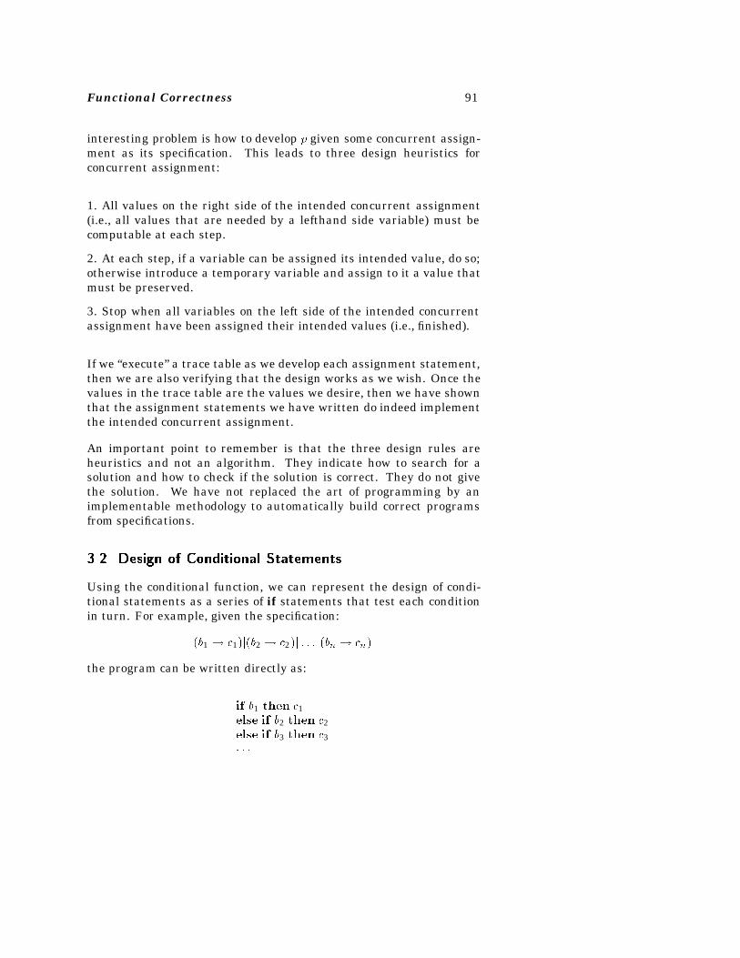
Functional Correctness 91
interesting problem is how to develop p given some concurrent assign-ment as its specification. This leads to three design heuristics forconcurrent assignment:
1. All values on the right side of the intended concurrent assignment(i.e., all values that are needed by a lefthand side variable) must becomputable at each step.
2. At each step, if a variable can be assigned its intended value, do so;otherwise introduce a temporary variable and assign to it a value thatmust be preserved.
3. Stop when all variables on the left side of the intended concurrentassignment have been assigned their intended values (i.e., finished).
If we “execute” a trace table as we develop each assignment statement,then we are also verifying that the design works as we wish. Once thevalues in the trace table are the values we desire, then we have shownthat the assignment statements we have written do indeed implementthe intended concurrent assignment.
An important point to remember is that the three design rules areheuristics and not an algorithm. They indicate how to search for asolution and how to check if the solution is correct. They do not givethe solution. We have not replaced the art of programming by animplementable methodology to automatically build correct programsfrom specifications.
���� Design of Conditional Statements
Using the conditional function, we can represent the design of condi-tional statements as a series of if statements that test each conditionin turn. For example, given the specification:
�b1 � c1�j�b2 � c2�j � � � j�bn � cn�
the program can be written directly as:
if b1 then c1else if b2 then c2else if b3 then c3� � �
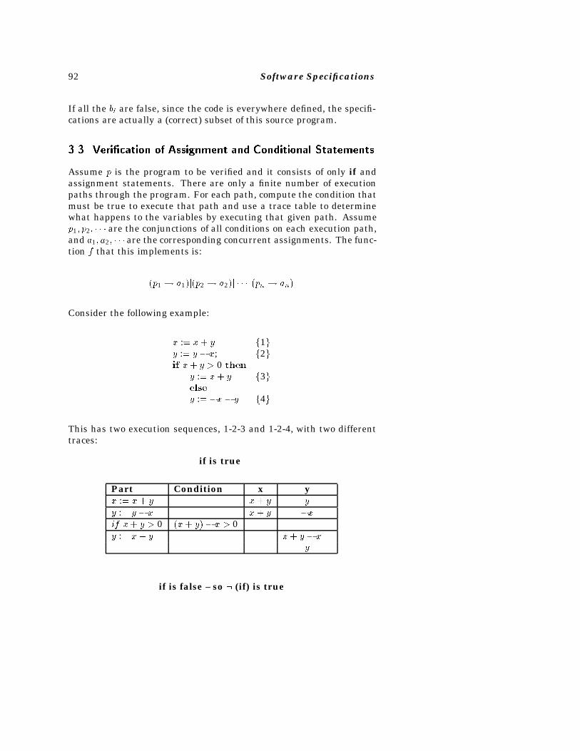
92 Software Specifications
If all the bi are false, since the code is everywhere defined, the specifi-cations are actually a (correct) subset of this source program.
���� Veri�cation of Assignment and Conditional Statements
Assume p is the program to be verified and it consists of only if andassignment statements. There are only a finite number of executionpaths through the program. For each path, compute the condition thatmust be true to execute that path and use a trace table to determinewhat happens to the variables by executing that given path. Assumep1� p2� � � � are the conjunctions of all conditions on each execution path,and a1� a2� � � � are the corresponding concurrent assignments. The func-tion f that this implements is:
�p1 � a1�j�p2 � a2�j � � � j�pn � an�
Consider the following example:
x :� x� y f1gy :� y � x; f2gif x� y � 0 then
y :� x� y f3gelse
y :� �x � y f4g
This has two execution sequences, 1-2-3 and 1-2-4, with two differenttraces:
if is true
Part Condition x yx :� x� y x� y y
y :� y � x x� y �xif x� y � 0 �x� y� � x � 0y :� x� y x� y � x �
y
if is false – so � (if) is true
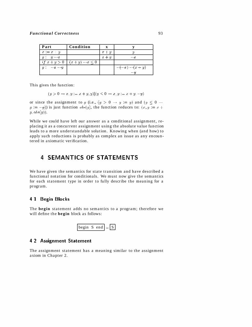
Functional Correctness 93
Part Condition x yx :� x� y x� y y
y :� y � x x� y �xif x� y � 0 �x� y� � x � 0y :� �x� y ���x� � �x� y� �
�y
This gives the function:
�y � 0 � x� y :� x� y� y�j�y � 0 � x� y :� x� y��y�
or since the assignment to y (i.e., �y � 0 � y :� y� and �y � 0 �y :� �y�) is just function abs�y�, the function reduces to: �x� y :� x �y� abs�y��.
While we could have left our answer as a conditional assignment, re-placing it as a concurrent assignment using the absolute value functionleads to a more understandable solution. Knowing when (and how) toapply such reductions is probably as complex an issue as any encoun-tered in axiomatic verification.
�� SEMANTICS OF STATEMENTS
We have given the semantics for state transition and have described afunctional notation for conditionals. We must now give the semanticsfor each statement type in order to fully describe the meaning for aprogram.
���� Begin Blocks
The begin statement adds no semantics to a program; therefore wewill define the begin block as follows:
begin S end � S
���� Assignment Statement
The assignment statement has a meaning similar to the assignmentaxiom in Chapter 2.
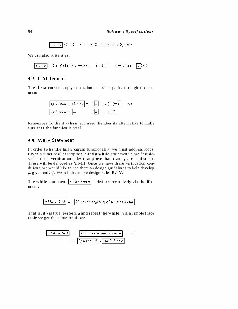
94 Software Specifications
x :� y �s� � f�i� j� j �i� j� � s i �� xg � f�x� y�g
We can also write it as:
x :� y � f�s� s�� j �i �� x� s��i� � s�i�� j �i � x� s��x� � y �s�g
���� If Statement
The if statement simply traces both possible paths through the pro-gram:
if b then s1 else s2 � � b � s1� j �� b � s2�
if b then s1 � � b � s1� j ��
Remember for the if - then, you need the identity alternative to makesure that the function is total.
���� While Statement
In order to handle full program functionality, we must address loops.Given a functional description f and a while statement p, we first de-scribe three verification rules that prove that f and p are equivalent.These will be denoted as V.I-III. Once we have these verification con-ditions, we would like to use them as design guidelines to help developp, given only f . We call these five design rules B.I-V.
The while statement while b do d is defined recursively via the if tomean:
while b do d � if b then begin d;while b do d end
That is, if b is true, perform d and repeat the while. Via a simple tracetable we get the same result as:
while b do d � if b then d;while b do d ����
� if b then d while b do d
Functional Correctness 95
Let f be the meaning of the while statement, that is, f � while b do d .By substituting back into (**) above, we get the first condition that:
V.If � if b then d f
What other conditions on f insure that it is indeed the specification ofthe while statement? If f is undefined for some input x, then bothsides of the equation are undefined. In order to insure that this cannothappen, we require that f is defined whenever while is defined, orthat domain� while � � domain�f�. (Note: For ease in reading, we willuse while to stand for while b do d .)
Similarly, if while is everywhere the identity function then any f
will fulfill the equation, because, if while is everywhere the identity,then similarly if b then d must also be the identity and the recursiveequation reduces to f � �� f � f . Thus we must also have domain�f� �domain� while �. This yields:
V.IIdomain�f� � domain� while b do d �
Consider any state s � domain� while �. If b �s� is true, that is, ex-pression b in state s is true, then from (**), s1 � d �s� and s1 �
domain� while �. This will be true, for s2� s3� � � � until at some point,b �sn� is false and both if b then d �sn� and while b do d �sn� equal sn.
This sn is a member of domain� while � and of range� while ). Moreimportantly, if b �s� evaluates to false, then while �s� � s, or statedanother way, while �s� � s for all states s where b �s� is false. Thisis just a restriction on the while function to those states where b isfalse, which is the function ���b� � while �. This must be equal tothe identity function () also restricted to the same domain, or just:���b� � �� �. Any candidate function f must also have this property,yielding the third constraint:
V.III��b� f� � ��b� ���
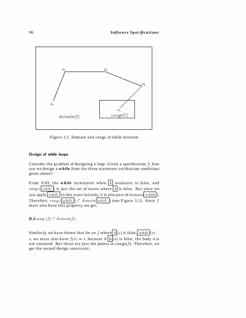
96 Software Specifications
��������
aaaaaaaaaa�
��
���
range�f�domain�f�
s5
s4
s3s2
s1
Figure 3.1. Domain and range of while function
Design of while loops
Consider the problem of designing a loop. Given a specification f , howcan we design a while from the three statement verification conditionsgiven above?
From V.III, the while terminates when b evaluates to false, andrange� while � is just the set of states where b is false. But since wecan apply while to this state initially, it is also part of domain� while �.Therefore, range� while � � domain� while � (see Figure 3.1). Since fmust also have this property, we get:
D.Irange�f� � domain�f�.
Similarly, we have shown that for an f where b �s� is false, while �s� �
s, we must also have f�s� � s, because if b �s� is false, the body d isnot executed. But these are just the points in range(f). Therefore, weget the second design constraint:
Functional Correctness 97
D.IIif s � range�f�� then f�s� � s.
D.I and D.II must be true if f is the meaning of a while statement.Therefore they show the existence of a possible solution. From D.II,we know f must be an identity on range�f� in order to be implementedwith a while. We can restate this as:
D.III b evaluates to true in domain�f��range�f� and false in range�f�.
Similarly to the assignment design, we develop the while loop via:
� D.IV Develop d so that all values are preserved for f .
� D.V Show that f is everywhere defined, that is, the loop must termi-nate for all x � domain�f�.
Given function f we develop a while statement such that while � fas follows:
� Existence. Verify conditions D.I and D.II. If these cannot be satis-fied, then no such while statement can be written.
� Range determination. Use D.III to develop some predicate b suchthat b is false on range�f� and true on domain�f� � range�f�. Since fand while are to be the same function, b becomes the predicate for theloop.
� Loop body. Use D.IV to develop an appropriate d. These guidelinesdo not give absolute solutions to this problem but do indicate how toverify whether the d is a solution once found. It is comparable to findingthe loop invariant in an axiomatic proof.
� Termination. Prove that the selected b and d causes the loop toterminate (condition D.V.). If proven that the loop terminates, andsince the second step shows that b �x� is false for x � range�f�, thisshows that the loop will terminate with some x in this range.
98 Software Specifications
�� USE OF FUNCTIONAL MODEL
���� Example� Veri�cation
Show that the function f � �A � B � A�B :� �B � �B �A�2�� �B ��B �A�2�j��� is implemented by the source program:
1 while A � B do2 begin3 A :� A� 1;4 if A � B then5 B :� B � 16 end
where A and B are integers and division means integer trun-cated division (e.g., 12 � 0).
The approach we follow is to first determine the functionality of theassignment statement (line 3), then the if statement (lines 4-5), thenthe entire begin block (lines 2-6) and finally the functionality of theentire segment (lines 1-6).
1. Line 3. A :� A � 1.
This is just the concurrent assignment: �A :� A � 1�.
2. Lines 4-5. d1 � if A � B then B :� B � 1
If A � B is true, evaluate the function B :� B�1, and if it is false, skipthe then statement and do nothing, e.g., the Identity function. Theconditional assignment can be written as:
d1 � �A � B � B :� B � 1�j��
3. Lines 2-6. d2 � begin A :� A � 1; if A � B then B :� B � 1 end
d2 � A:=A+1 if A<B then B:=B-1� �A :� A� 1� d1� �A :� A� 1� ��A � B � B :� B � 1�j���
Develop a trace table for the begin block. There will be two pathsthrough this block (e.g., first alternative for d1 and second), and hencethere will be two trace tables:
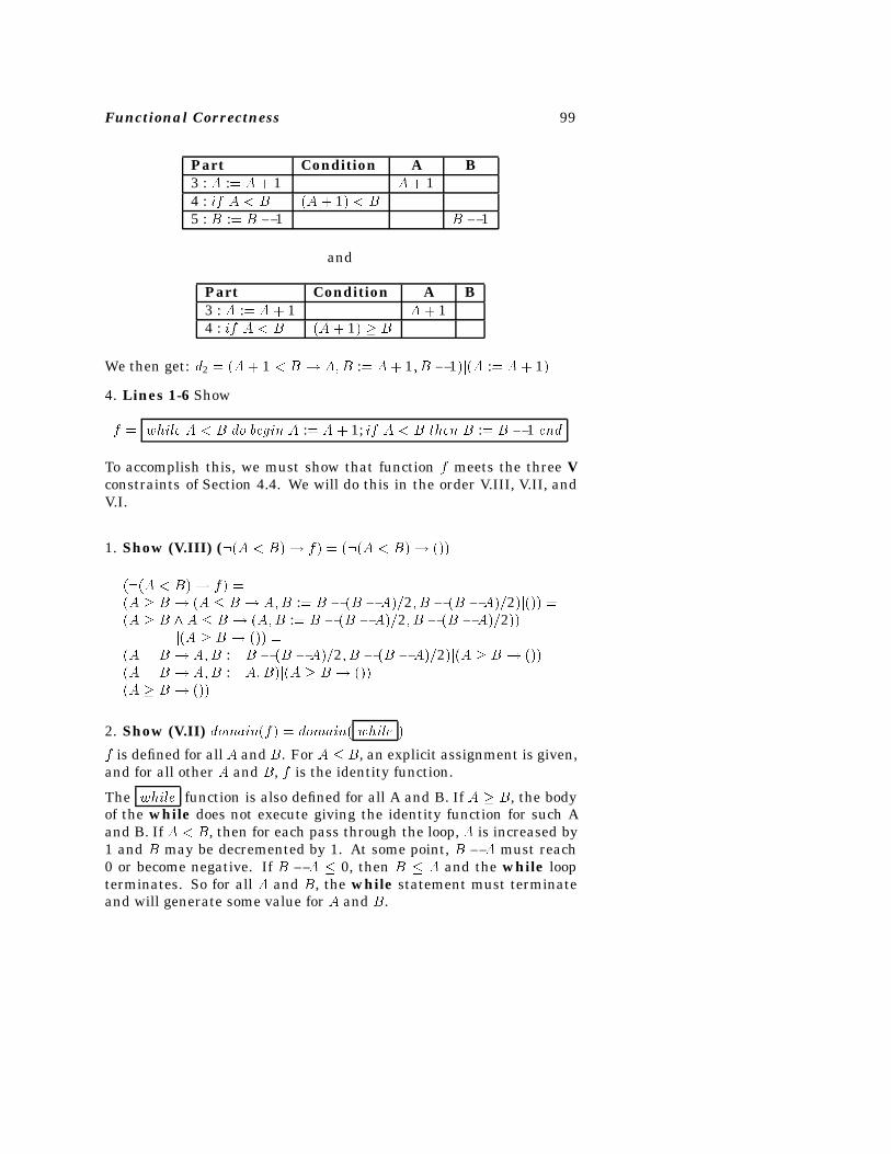
Functional Correctness 99
Part Condition A B3 : A :� A � 1 A� 14 : if A � B �A � 1� � B5 : B :� B � 1 B � 1
and
Part Condition A B3 : A :� A � 1 A � 14 : if A � B �A � 1� � B
We then get: d2 � �A� 1 � B � A�B :� A� 1� B � 1�j�A :� A � 1�
4. Lines 1-6 Show
f � while A � B do begin A :� A � 1; if A � B then B :� B � 1 end
To accomplish this, we must show that function f meets the three Vconstraints of Section 4.4. We will do this in the order V.III, V.II, andV.I.
1. Show (V.III) (��A � B� � f� � ���A � B� � ���
���A � B� � f� ��A � B � �A � B � A�B :� B � �B � A�2� B � �B �A�2�j��� ��A � B A � B � �A�B :� B � �B � A�2� B � �B � A�2��
j�A � B � ��� ��A � B � A�B :� B � �B �A�2� B � �B � A�2�j�A � B � ��� ��A � B � A�B :� A�B�j�A � B � ��� ��A � B � ���
2. Show (V.II) domain�f� � domain� while �
f is defined for all A and B. For A � B, an explicit assignment is given,and for all other A and B, f is the identity function.
The while function is also defined for all A and B. If A � B, the bodyof the while does not execute giving the identity function for such Aand B. If A � B, then for each pass through the loop, A is increased by1 and B may be decremented by 1. At some point, B � A must reach0 or become negative. If B � A � 0, then B � A and the while loopterminates. So for all A and B, the while statement must terminateand will generate some value for A and B.
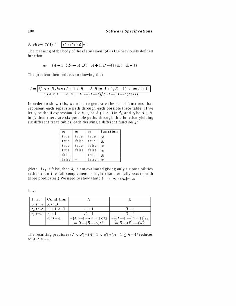
100 Software Specifications
3. Show (V.I) f � if b then d f
The meaning of the body of the if statement (4) is the previously definedfunction:
d2 � �A� 1 � B � A�B :� A� 1� B � 1�j�A :� A � 1�
The problem then reduces to showing that:
f � if A � B then �A� 1 � B � A�B :� A� 1� B � 1�j�A :� A � 1� ��A � B � A�B :� B � �B �A�2� B � �B � A�2�j���
In order to show this, we need to generate the set of functions thatrepresent each separate path through each possible trace table. If welet c1 be the if expression A � B, c2 be A� 1 � B in d2, and c3 be A � Bin f , then there are six possible paths through this function yieldingsix different trace tables, each deriving a different function gi:
c1 c2 c3 functiontrue true true g1true false true g2true true false g3true false false g4false – true g5false – false g6
(Note, if c1 is false, then d2 is not evaluated giving only six possibilitiesrather than the full complement of eight that normally occurs withthree predicates.) We need to show that: f � g1jg2jg3jg4jg5jg6
1. g1
Part Condition A B
c1 true A � Bc2 true A � 1 � B A � 1 B � 1c3 true A � 1 B � 1 B � 1
� B � 1 ��B � 1 � �A � 1��2 ��B � 1� �A� 1��2� B � �B �A�2 � B � �B � A�2
The resulting predicate �A � B� �A�1 � B� �A�1 � B�1� reducesto A � B � 1.
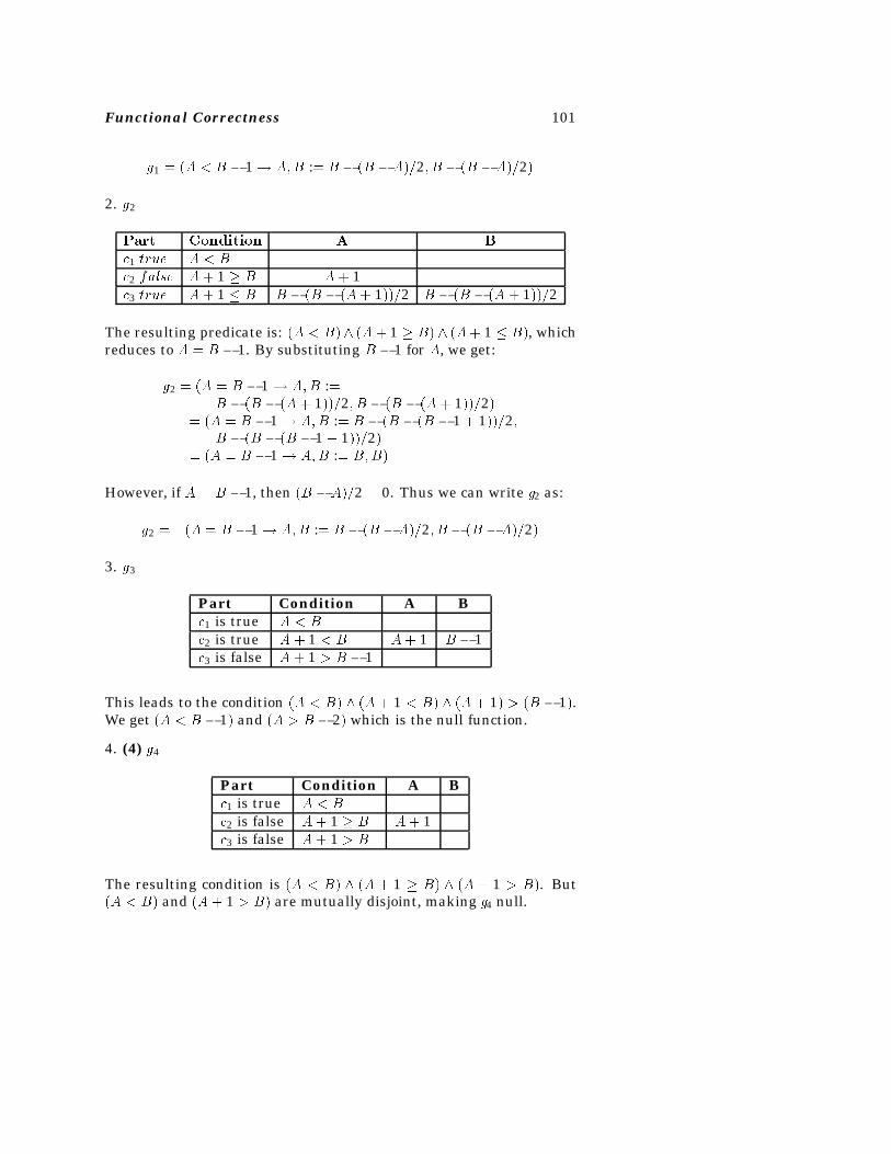
Functional Correctness 101
g1 � �A � B � 1 � A�B :� B � �B �A�2� B � �B �A�2�
2. g2
Part Condition A B
c1 true A � Bc2 false A� 1 � B A � 1c3 true A� 1 � B B � �B � �A� 1��2 B � �B � �A � 1��2
The resulting predicate is: �A � B� �A� 1 � B� �A� 1 � B�, whichreduces to A � B � 1. By substituting B � 1 for A, we get:
g2 � �A � B � 1 � A�B :�B � �B � �A� 1��2� B � �B � �A � 1��2�
� �A � B � 1 � A�B :� B � �B � �B � 1 � 1��2�B � �B � �B � 1 � 1��2�
� �A � B � 1 � A�B :� B�B�
However, if A � B � 1, then �B � A�2 � 0. Thus we can write g2 as:
g2 � �A � B � 1 � A�B :� B � �B �A�2� B � �B �A�2�
3. g3
Part Condition A Bc1 is true A � B
c2 is true A � 1 � B A� 1 B � 1c3 is false A � 1 � B � 1
This leads to the condition �A � B� �A � 1 � B� �A � 1� � �B � 1�.We get �A � B � 1� and �A � B � 2� which is the null function.
4. (4) g4
Part Condition A Bc1 is true A � B
c2 is false A� 1 � B A� 1c3 is false A� 1 � B
The resulting condition is �A � B� �A � 1 � B� �A � 1 � B�. But�A � B� and �A� 1 � B� are mutually disjoint, making g4 null.
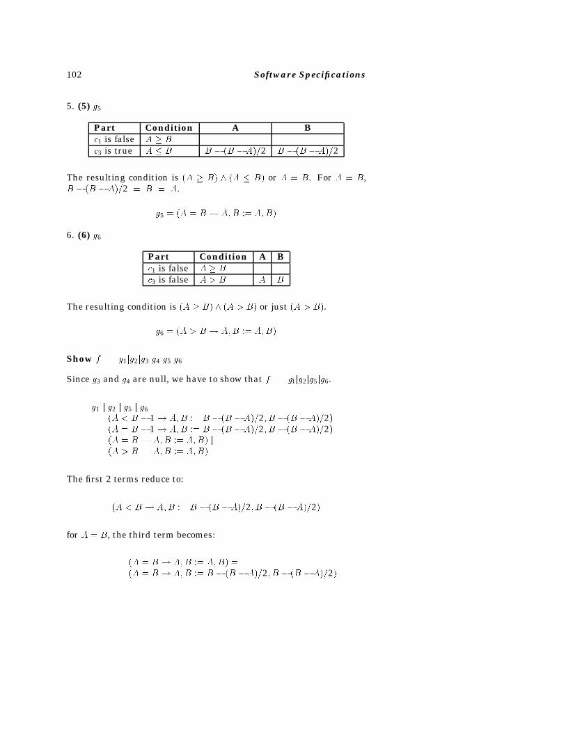
102 Software Specifications
5. (5) g5
Part Condition A Bc1 is false A � B
c3 is true A � B B � �B �A�2 B � �B � A�2
The resulting condition is �A � B� �A � B� or A � B. For A � B,B � �B � A�2 � B � A.
g5 � �A � B � A�B :� A�B�
6. (6) g6
Part Condition A Bc1 is false A � Bc3 is false A � B A B
The resulting condition is �A � B� �A � B� or just �A � B�.
g6 � �A � B � A�B :� A�B�
Show f � g1jg2jg3jg4jg5jg6
Since g3 and g4 are null, we have to show that f � g1jg2jg5jg6.
g1 j g2 j g5 j g6 ��A � B � 1 � A�B :� B � �B � A�2� B � �B � A�2� j�A � B � 1 � A�B :� B � �B � A�2� B � �B � A�2� j�A � B � A�B :� A�B� j�A � B � A�B :� A�B�
The first 2 terms reduce to:
�A � B � A�B :� B � �B �A�2� B � �B � A�2�
for A � B, the third term becomes:
�A � B � A�B :� A�B� ��A � B � A�B :� B � �B �A�2� B � �B � A�2�
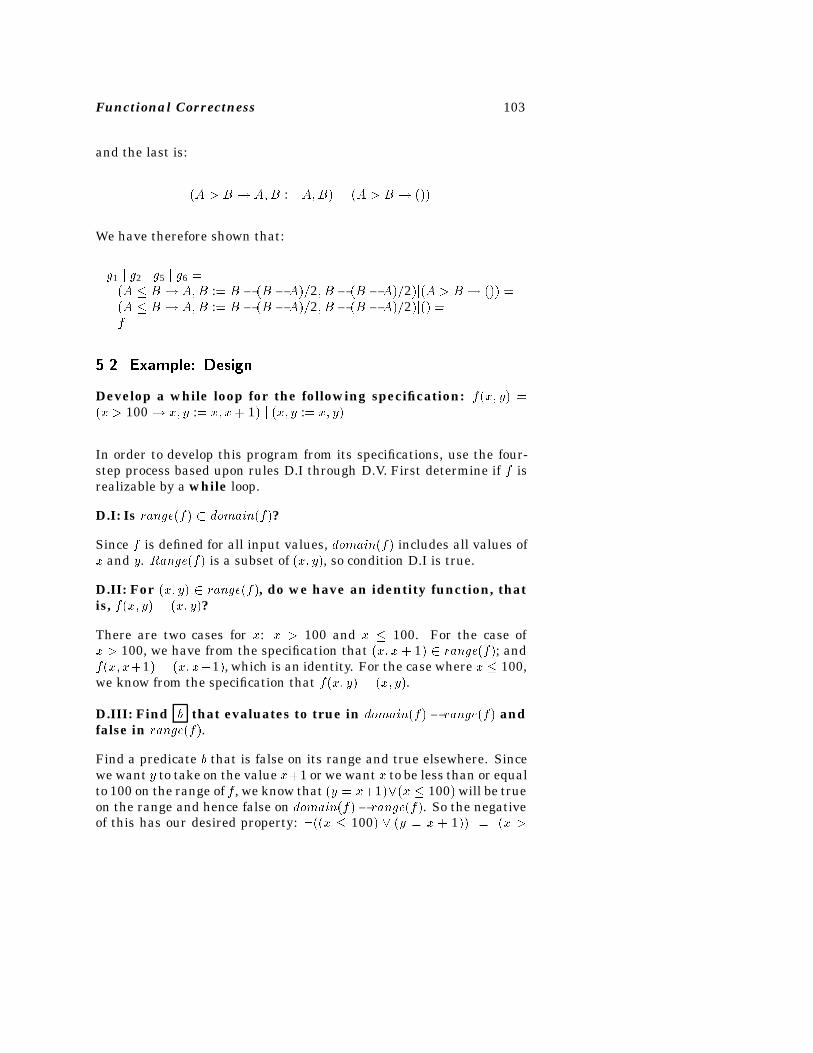
Functional Correctness 103
and the last is:
�A � B � A�B :� A�B� � �A � B � ���
We have therefore shown that:
g1 j g2 j g5 j g6 ��A � B � A�B :� B � �B � A�2� B � �B � A�2�j�A � B � ��� ��A � B � A�B :� B � �B � A�2� B � �B � A�2�j�� �f
���� Example� Design
Develop a while loop for the following specification: f�x� y� ��x � 100 � x� y :� x� x� 1� j �x� y :� x� y�
In order to develop this program from its specifications, use the four-step process based upon rules D.I through D.V. First determine if f isrealizable by a while loop.
D.I: Is range�f� � domain�f�?
Since f is defined for all input values, domain�f� includes all values ofx and y. Range�f� is a subset of �x� y�, so condition D.I is true.
D.II: For �x� y� � range�f�, do we have an identity function, thatis, f�x� y� � �x� y�?
There are two cases for x: x � 100 and x � 100. For the case ofx � 100, we have from the specification that �x� x� 1� � range�f�; andf�x� x�1� � �x� x�1�, which is an identity. For the case where x � 100,we know from the specification that f�x� y� � �x� y�.
D.III: Find b that evaluates to true in domain�f� � range�f� andfalse in range�f�.
Find a predicate b that is false on its range and true elsewhere. Sincewe want y to take on the value x�1 or we want x to be less than or equalto 100 on the range of f , we know that �y � x�1���x � 100� will be trueon the range and hence false on domain�f�� range�f�. So the negativeof this has our desired property: ���x � 100� � �y � x � 1�� � �x �
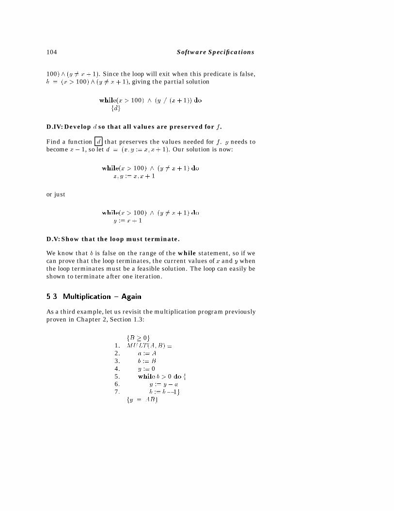
104 Software Specifications
100� �y �� x� 1�. Since the loop will exit when this predicate is false,b � �x � 100� �y �� x� 1�, giving the partial solution
while�x � 100� �y �� �x� 1�� dofdg
D.IV: Develop d so that all values are preserved for f .
Find a function d that preserves the values needed for f . y needs tobecome x� 1, so let d � �x� y :� x� x� 1�. Our solution is now:
while�x � 100� �y �� x� 1� dox� y :� x� x� 1
or just
while�x � 100� �y �� x� 1� doy :� x� 1
D.V: Show that the loop must terminate.
We know that b is false on the range of the while statement, so if wecan prove that the loop terminates, the current values of x and y whenthe loop terminates must be a feasible solution. The loop can easily beshown to terminate after one iteration.
���� Multiplication Again
As a third example, let us revisit the multiplication program previouslyproven in Chapter 2, Section 1.3:
fB � 0g1� MULT �A�B� �2� a :� A3� b :� B4� y :� 05� while b � 0 do f6� y :� y � a7� b :� b� 1g
fy � ABg
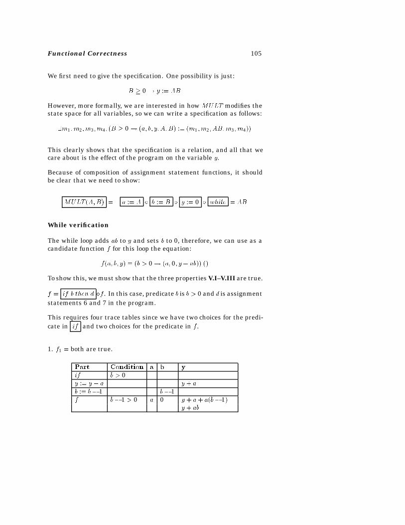
Functional Correctness 105
We first need to give the specification. One possibility is just:
B � 0 � y :� AB
However, more formally, we are interested in how MULT modifies thestate space for all variables, so we can write a specification as follows:
�m1�m2�m3�m4� �B � 0 � �a� b� y� A�B� :� �m1�m2� AB�m3�m4��
This clearly shows that the specification is a relation, and all that wecare about is the effect of the program on the variable y.
Because of composition of assignment statement functions, it shouldbe clear that we need to show:
MULT �A�B� � a :� A b :� B y :� 0 while � AB
While verification
The while loop adds ab to y and sets b to 0, therefore, we can use as acandidate function f for this loop the equation:
f�a� b� y� � �b � 0 � �a� 0� y � ab��j��
To show this, we must show that the three properties V.I–V.III are true.
f � if b then d f . In this case, predicate b is b � 0 and d is assignmentstatements 6 and 7 in the program.
This requires four trace tables since we have two choices for the predi-cate in if and two choices for the predicate in f .
1. f1 � both are true.
Part Condition a b y
if b � 0y :� y � a y � a
b :� b� 1 b� 1f b� 1 � 0 a 0 y � a� a�b� 1� �
y � ab
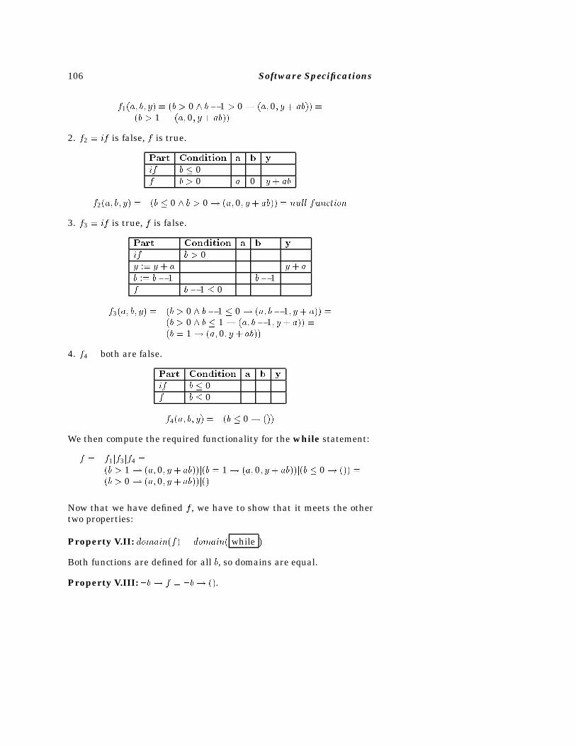
106 Software Specifications
f1�a� b� y� � �b � 0 b� 1 � 0 � �a� 0� y � ab�� ��b � 1 � �a� 0� y � ab��
2. f2 � if is false, f is true.
Part Condition a b y
if b � 0f b � 0 a 0 y � ab
f2�a� b� y� � �b � 0 b � 0 � �a� 0� y � ab�� � null function
3. f3 � if is true, f is false.
Part Condition a b y
if b � 0y :� y � a y � a
b :� b� 1 b� 1f b � 1 � 0
f3�a� b� y� � �b � 0 b� 1 � 0 � �a� b� 1� y � a�� ��b � 0 b � 1 � �a� b� 1� y � a�� ��b � 1 � �a� 0� y � ab��
4. f4 � both are false.
Part Condition a b y
if b � 0f b � 0
f4�a� b� y� � �b � 0 � ���
We then compute the required functionality for the while statement:
f � f1jf3jf4 ��b � 1 � �a� 0� y � ab��j�b � 1 � �a� 0� y � ab��j�b � 0 � ��� ��b � 0 � �a� 0� y � ab��j��
Now that we have defined f , we have to show that it meets the othertwo properties:
Property V.II: domain�f� � domain� while �
Both functions are defined for all b, so domains are equal.
Property V.III: �b� f � �b� ��.
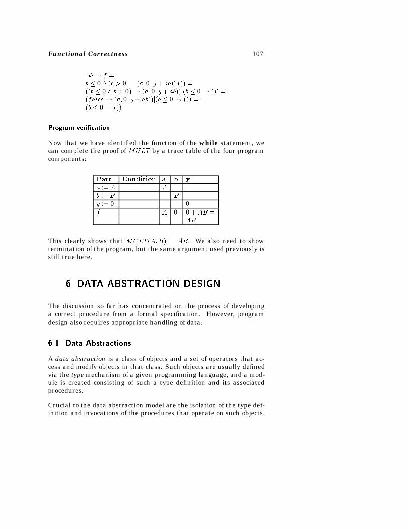
Functional Correctness 107
�b� f �b � 0 �b � 0 � �a� 0� y � ab��j��� ���b � 0 b � 0� � �a� 0� y � ab��j�b � 0 � ��� ��false � �a� 0� y � ab��j�b � 0 � ��� ��b � 0 � ���
Program veri�cation
Now that we have identified the function of the while statement, wecan complete the proof of MULT by a trace table of the four programcomponents:
Part Condition a b y
a :� A Ab :� B By :� 0 0f A 0 0 � AB �
AB
This clearly shows that MULT �A�B� � AB. We also need to showtermination of the program, but the same argument used previously isstill true here.
�� DATA ABSTRACTION DESIGN
The discussion so far has concentrated on the process of developinga correct procedure from a formal specification. However, programdesign also requires appropriate handling of data.
���� Data Abstractions
A data abstraction is a class of objects and a set of operators that ac-cess and modify objects in that class. Such objects are usually definedvia the type mechanism of a given programming language, and a mod-ule is created consisting of such a type definition and its associatedprocedures.
Crucial to the data abstraction model are the isolation of the type def-inition and invocations of the procedures that operate on such objects.
108 Software Specifications
Each procedure has a well-defined input-output definition. The im-plementor is free to modify any procedure within a module as long asits input-output functional behavior is preserved, and any use of sucha procedure can only assume its functional specification. The resultof this is that rather than viewing a program as a complex interac-tion among many objects and procedures, a program can be viewed asthe interaction among a small set of data abstractions, each relativelysmall and well-defined.
Languages such as Ada (or C++) allow data abstractions to be built rel-atively easily, since the object type can be specified as the private partof a package (or class) specification. Only the body of the packagehas access to the type structure while other modules have access onlyto the names of the procedures that are contained in the module.
However, even in older languages, such as C or Pascal, data abstrac-tions form a good model of program design. Even though not automat-ically supported by the language, with reasonable care, programs canbe designed which adhere to the data abstraction guidelines.
���� Representation Functions
A procedure within a data abstraction translates a high-level descrip-tion of a process into a lower-level programming language implemen-tation. For example, suppose character strings up to some predefinedmaximum value are needed. Pascal, for example, only defines fixed-length strings; therefore, we must implement this as objects usingprimitive Pascal data types.
In procedures outside of the defining module, we would like to refer tothese objects (e.g., call them Vstrings) and be able to operate on them,while inside the module we need to operate on their Pascal representa-tion (arrays of characters). In the former case, we call such functionsabstract functions that define the functional behavior of the opera-tion, while we call the latter case concrete functions that give thedetails of the implementation.
For the Vstring example, we could define such a string via an abstractcomment containing the functional definition:
fabs : xabs � � x1� x2� � � �xn �g
Functional Correctness 109
while the concrete representation of a Vstring could be:
con : xcon : recordchars : array�1��maxval� of char;size : 0��maxvalend;
To show that both representations are the same, we define a represen-tation function which maps concrete objects into abstract objects bymapping a state into a similar state leaving all data unchanged exceptfor those specific objects. Let r map a concrete object into its abstractrepresentation. If Cstrings is the set of concrete strings (i.e., the setof variables defined by the above record description) and if Vstrings isthe set of abstract strings, then we define a representation function rwith the signature: r : state� state such that
r�� f�u� v�ju � v except that if u�x� � Cstrings� then v�x� � V strings g
We simply mean that u and v represent the same set of variables in theprogram store, except that each occurrence of a concrete variable in uis replaced by its abstract definition in v.
For each implementation of a string, we have its abstract meaninggiven by function r:
xabs :�� xcon�chars�i�j1 � i � xcon�size �
The purpose of a procedure in an abstraction module is to implementan abstract function on this abstract data. For example, if we wouldlike to implement an Append operation, we can define x :� Append�x� y�as:
fabs : x1� � � � � xn� � � � � xn�m :� x1� � � �xn� y1� � � � � ymg
Similarly, we can define a concrete implementation of this same func-tion as:
fcon : x�chars�n� 1�� � � � � x�chars�n�m�� x�size :�y�chars�1�� � � � � y�chars�y�size�� x�size � y�sizeg
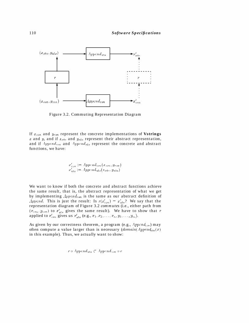
110 Software Specifications
�
�
��
��
�
�
x�abs
x�con�xcon� ycon�
�xabs� yabs� Appendabs
Appendcon
rr
Figure 3.2. Commuting Representation Diagram
If xcon and ycon represent the concrete implementations of Vstringsx and y, and if xabs and yabs represent their abstract representation,and if Appendcon and Appendabs represent the concrete and abstractfunctions, we have:
x�con :� Appendcon�xcon� ycon�x�abs :� Appendabs�xabs� yabs�
We want to know if both the concrete and abstract functions achievethe same result, that is, the abstract representation of what we getby implementing Appendcon is the same as our abstract definition ofAppend. This is just the result: Is r�x�con� � x�abs? We say that therepresentation diagram of Figure 3.2 commutes (i.e., either path from�xcon� ycon� to x�abs gives the same result). We have to show that rapplied to x�con gives us x�abs (e.g., x1� x2� � � � � xn� y1� � � � � ym�.
As given by our correctness theorem, a program (e.g., Appendcon) mayoften compute a value larger than is necessary (domain�Appendabs�x�in this example). Thus, we actually want to show:
r Appendabs � Appendcon r
Functional Correctness 111
�� USING FUNCTIONAL VERIFICATION
We have seemingly developed two mechanisms for designing programs:(a) a functional model for showing the equivalence of a design andits implementation, and (b) a commuting diagram for showing correctdata abstractions. However, both are complementary ideas of the sametheory. For example, the concrete design comment for Append in theprevious section is just a concurrent assignment which we can translateinto a source program via the techniques described earlier.
This leads to a strategy for developing correct programs:
1. From the requirements of a program, develop the abstract data ob-jects that are needed.
2. For each object, develop abstract functions that may be necessary tooperate on the abstract object.
3. Using the abstract object and operations as a goal, design the con-crete representation of the object and corresponding representationfunction.
4. Design a concrete function for each corresponding abstract function.
5. Show that the representation diagram commutes. That is, the con-crete function does indeed implement the abstract function.
6. Develop correct programs from each concrete function.
Note the order of Steps 2 and 3. It is important to understand theabstract functions before one designs the concrete representation, sincethe appropriate representation will depend greatly on the application.Consider the implementation of a date data object. The followingare all feasible concrete representations depending upon the requiredabstract functions:
� Store as character string ‘MM/DD/YY.’ This is appropriate if thedate is simply a unique tag associated with some data and has no othersemantic meaning.
� Store as � Y Y�DDD � where integer YY is the year and integerDDD is the day of year. This is quite efficient if sequential dates areneeded.
112 Software Specifications
� Store as number of days since some initial date. This is mostefficient to compute distances between two days. It also avoids certainproblems such as accounting for leap years in all functions, but it iscumbersome to print out in its usual format.
� Store as � MM�DD� Y Y � for integers MM, DD, and YY. Com-puting dates is a bit more cumbersome, but conversion to its usualprinted form is quite easy.
The importance of this technique is that it can be applied at any levelof detail. Here, we obviously considered only short program segments.For larger programs, only those concepts that are critical to the successof a program need be formalized, although a long range goal would beto develop this or other techniques which can be applied to very largesystems in their entirety. Its major difference from other verificationtechniques is that it forces the programmer or designer to considerthe functionality of the program as a whole, and requires the designerto design data structures with operations that operate on those struc-tures. Since this is central to the data abstraction model of programdesign, this technique is quite applicable to current thinking aboutprogramming.
�� EXERCISES
Problem 1. It is not always the case that a while loop can be used toimplement a desired specification. Therefore, as designers it is impor-tant for us to know when a loop can and cannot be used:
Theorem: A while statement can be devised to implement a desiredspecification f if and only if
1. range�f� � domain�f�, and
2. f behaves as the identity function in range�f�.
In each of the following parts, a specification f is given, and you are tostate whether or not a while-loop construct can be devised to imple-ment that specification. If so, then give such a loop. If not, then justifyyour claim. In all cases, x and y are integer valued variables.
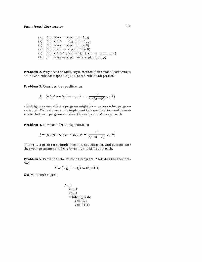
Functional Correctness 113
�a� f � �true� x� y :� x� 1� y��b� f � �x � 0 � x� y :� x� 1� y��c� f � �true� x� y :� x� y� 0��d� f � �y � 0 � x� y :� x� y� 0��e� f � �x � 0 y � 0 � ��� j �true� x� y :� y� x��f� f � �true� x� y :� max�x� y��min�x� y��
Problem 2. Why does the Mills’ style method of functional correctnessnot have a rule corresponding to Hoare’s rule of adaptation?
Problem 3. Consider the specification
f � �n � 0 n � k� x� n� k :�n!
k! � �n � k�!� n� k�
which ignores any effect a program might have on any other programvariables. Write a program to implement this specification, and demon-strate that your program satisfies f by using the Mills approach.
Problem 4. Now consider the specification
f � �n � 0 n � k� x� n� k :�n!
n! � �n � k�!� n� k�
and write a program to implement this specification, and demonstratethat your program satisfies f by using the Mills approach.
Problem 5. Prove that the following program P satisfies the specifica-tion
F � �n � 1 � t� i :� n!� n� 1�
Use Mills’ techniques.
P � ft :� 1i :� 1while i � n do
t :� t � ii :� i � 1g
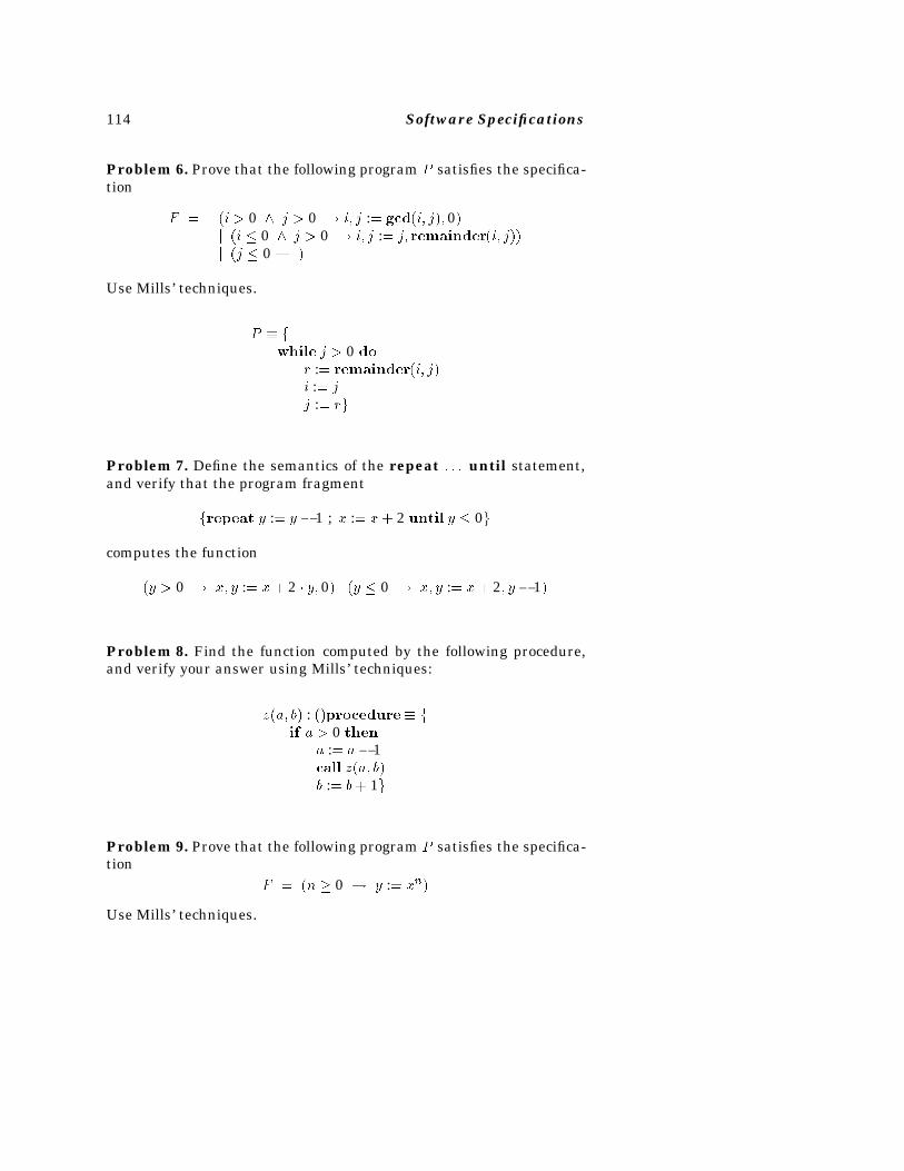
114 Software Specifications
Problem 6. Prove that the following program P satisfies the specifica-tion
F � �i � 0 j � 0 � i� j :� gcd�i� j�� 0�j �i � 0 j � 0 � i� j :� j� remainder�i� j��j �j � 0 � �
Use Mills’ techniques.
P � fwhile j � 0 do
r :� remainder�i� j�i :� jj :� rg
Problem 7. Define the semantics of the repeat � � � until statement,and verify that the program fragment
frepeat y :� y � 1 ; x :� x� 2 until y � 0g
computes the function
�y � 0 � x� y :� x� 2 � y� 0� j �y � 0 � x� y :� x� 2� y � 1�
Problem 8. Find the function computed by the following procedure,and verify your answer using Mills’ techniques:
z�a� b� : ��procedure � fif a � 0 then
a :� a � 1call z�a� b�b :� b� 1g
Problem 9. Prove that the following program P satisfies the specifica-tion
F � �n � 0 � y :� xn�
Use Mills’ techniques.
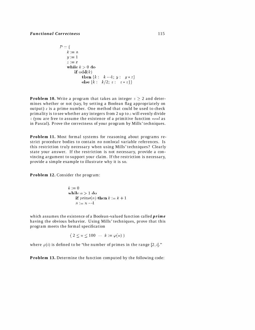
Functional Correctness 115
P � fk :� ny :� 1z :� xwhile k � 0 do
if odd�k�then fk :� k � 1; y :� y � zgelse fk :� k2; z :� z � zgg
Problem 10. Write a program that takes an integer z � 2 and deter-mines whether or not (say, by setting a Boolean flag appropriately onoutput) z is a prime number. One method that could be used to checkprimality is to see whether any integers from 2 up to z will evenly dividez (you are free to assume the existence of a primitive function mod asin Pascal). Prove the correctness of your program by Mills’ techniques.
Problem 11. Most formal systems for reasoning about programs re-strict procedure bodies to contain no nonlocal variable references. Isthis restriction truly necessary when using Mills’ techniques? Clearlystate your answer. If the restriction is not necessary, provide a con-vincing argument to support your claim. If the restriction is necessary,provide a simple example to illustrate why it is so.
Problem 12. Consider the program:
k :� 0while n � 1 do
if prime�n� then k :� k � 1n :� n� 1
which assumes the existence of a Boolean-valued function called primehaving the obvious behavior. Using Mills’ techniques, prove that thisprogram meets the formal specification
� 2 � n � 100 � k :� ��n� �
where ��i� is defined to be “the number of primes in the range �2� i�.”
Problem 13. Determine the function computed by the following code:

116 Software Specifications
while x �� 0 dot :� 0while t �� y do
s :� s� 1x :� x� 3t :� t � 1y :� y � x
x :� x� 1
Problem 14. Write a program whose function exactly equals the fol-lowing specification:
� 2 � n � 5 � x :� prime�n� �
where in this case, our function prime�i� returns the ith prime num-ber (for example, prime�1� � 2 and prime�7� � 17). Verify that yourprogram behaves exactly like the specification using Mills’ techniques.
Problem 15. Determine the function computed by the following proce-dure, and prove it is so by Mills’ techniques:
mystery procedure �x� n� z� : �� � fif n � 0 then
z :� 1else
n :� n� 1callmystery�x� n� z� : ��x :� 2xz :� 2g
Problem 16. Consider the functional specification
f � �0 � n � k :� bits�n��
where bits(j) is defined as “the number of 1 bits used to represent theinteger j as a binary numeral.” (For instance, bits(1)�1, bits(8)�1,and bits(7)�3.)
Write a program that implements this specification. Verify the imple-mentation using Mills’ techniques.
Functional Correctness 117
� SUGGESTED READINGS
The first sections of the paper
� D.D. Dunlop and V.R. Basili, “A Comparative Analysis of FunctionalCorrectness,” ACM Computing Surveys, Vol. 14, No. 2, June 1982,pp. 229-244.
provide an especially useful introduction to this area. The originalworks, of course, are also invaluable:
� R.C. Linger, H.D. Mills and B.I. Witt, Structured Programming: The-ory and Practice, Addison-Wesley, Reading, MA, 1979, Chapter 6.
� H.D. Mills, “The New Math of Computer Programming, Communica-tions of the ACM, Vol. 18, No. 1, 1975, pp. 43-48.
The papers
� J.D. Gannon, R.B. Hamlet and H.D. Mills, “Theory of Modules,” IEEETransactions on Software Engineering, Vol. 13, No. 7, 1987, pp. 820-829.
� M. V. Zelkowitz, “A functional correctness model of program verifica-tion,” IEEE Computer, Vol. 23, No. 11, 1990, pp. 30-39.
are works that clarify many of the more subtle points associated withfunctional correctness. Finally, even though the material can not bedescribed as being compact, chapters 6–11 in
� H.D. Mills, V.R. Basili, J.D. Gannon and R.G. Hamlet, Principlesof Computer Programming: A Mathematical Approach, William C.Brown, Dubuque, IA, 1987.
provide a large number of exercises for students of the functional ap-proach.

118 Software Specifications
Chapter 4
Predicate Transformers
In work related to the Hoare-style axiomatic proof, Dijkstra developedthe concept of the weakest precondition [10]. Using the concept ofa state, much like in the functional model of Chapter 3, the idea ofthe weakest precondition is defined. In addition, Dijkstra consideredthe concept of nondeterminacy in programming languages with theintroduction of the guarded command. These simplify some of theverification properties we wish to prove.
�� GUARDED COMMANDS
Most programming languages (and algorithms) are sequential and de-terministic. For example, the symbolic trace table method of Chap-ter 3 is strictly based upon being able to trace the execution of a pro-gram statement by statement in a prescribed order. However, thereare times when nondeterminacy makes a software design easier. Un-fortunately, we have not had the programming tools for constructing“nondeterministic” programs in existing languages. We first describeseveral constructs for introducing nondeterminacy into languages andthen show how some algorithms become easier to describe using thismethod.
The basic concept is the guard which is written as: ��. IfB is a predicateand S is a statement, then in a guarded command, B � S means that
119
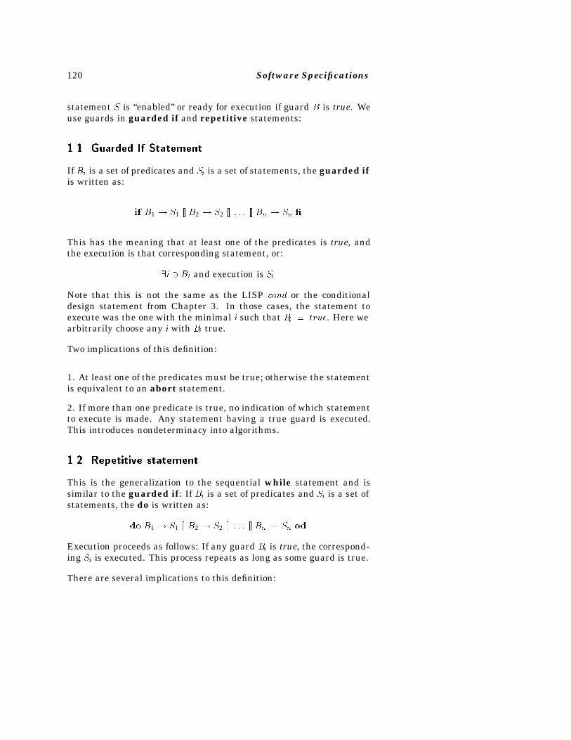
120 Software Specifications
statement S is “enabled” or ready for execution if guard B is true. Weuse guards in guarded if and repetitive statements:
���� Guarded If Statement
If Bi is a set of predicates and Si is a set of statements, the guarded ifis written as:
if B1 � S1 �� B2 � S2 �� � � � �� Bn � Sn �
This has the meaning that at least one of the predicates is true, andthe execution is that corresponding statement, or:
�i � Bi and execution is Si
Note that this is not the same as the LISP cond or the conditionaldesign statement from Chapter 3. In those cases, the statement toexecute was the one with the minimal i such that Bi � true. Here wearbitrarily choose any i with Bi true.
Two implications of this definition:
1. At least one of the predicates must be true; otherwise the statementis equivalent to an abort statement.
2. If more than one predicate is true, no indication of which statementto execute is made. Any statement having a true guard is executed.This introduces nondeterminacy into algorithms.
���� Repetitive statement
This is the generalization to the sequential while statement and issimilar to the guarded if: If Bi is a set of predicates and Si is a set ofstatements, the do is written as:
do B1 � S1 �� B2 � S2 �� � � � �� Bn � Sn od
Execution proceeds as follows: If any guard Bi is true, the correspond-ing Si is executed. This process repeats as long as some guard is true.
There are several implications to this definition:
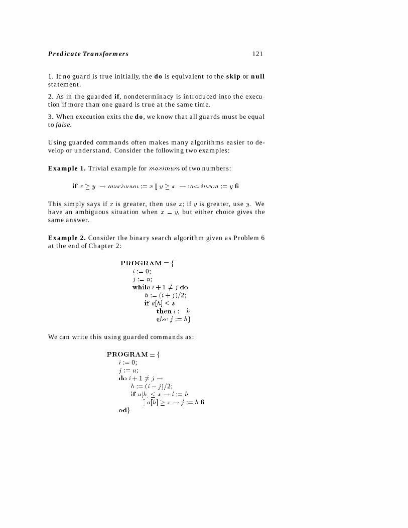
Predicate Transformers 121
1. If no guard is true initially, the do is equivalent to the skip or nullstatement.
2. As in the guarded if, nondeterminacy is introduced into the execu-tion if more than one guard is true at the same time.
3. When execution exits the do, we know that all guards must be equalto false.
Using guarded commands often makes many algorithms easier to de-velop or understand. Consider the following two examples:
Example 1. Trivial example for maximum of two numbers:
if x � y � maximum :� x �� y � x � maximum :� y �
This simply says if x is greater, then use x; if y is greater, use y. Wehave an ambiguous situation when x � y, but either choice gives thesame answer.
Example 2. Consider the binary search algorithm given as Problem 6at the end of Chapter 2:
PROGRAM � fi :� 0;j :� n;while i � 1 �� j do
h :� �i � j�2;if a�h� � x
then i :� he¯lse j :� hg
We can write this using guarded commands as:
PROGRAM � fi :� 0;j :� n;do i� 1 �� j �
h :� �i � j�2;if a�h� � x� i :� h
�� a�h� � x� j :� h �odg
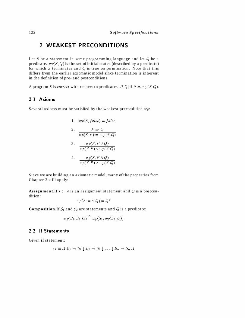
122 Software Specifications
�� WEAKEST PRECONDITIONS
Let S be a statement in some programming language and let Q be apredicate. wp�S�Q� is the set of initial states (described by a predicate)for which S terminates and Q is true on termination. Note that thisdiffers from the earlier axiomatic model since termination is inherentin the definition of pre- and postconditions.
A program S is correct with respect to predicates �P�Q� if P wp�S�Q�.
���� Axioms
Several axioms must be satisfied by the weakest precondition wp:
1� wp�S� false� � false
2� P Q
wp�S� P � wp�S�Q�
3� wp�S� P �Q�
wp�S� P � �wp�S�Q�
4� wp�S� P Q�
wp�S� P � wp�S�Q�
Since we are building an axiomatic model, many of the properties fromChapter 2 still apply:
Assignment.If x :� e is an assignment statement and Q is a postcon-dition:
wp�x :� e�Q� � Qxe
Composition.If S1 and S2 are statements and Q is a predicate:
wp�S1;S2� Q��� wp�S1� wp�S2� Q��
���� If Statements
Given if statement:
if � if B1 � S1 �� B2 � S2 �� � � � �� Bn � Sn �
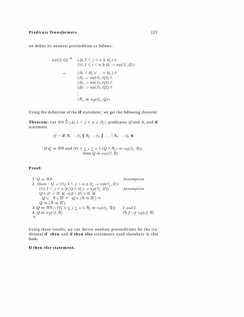
Predicate Transformers 123
we define its weakest precondition as follows:
wp�if�Q��� ��j� 1 � j � n � Bj�
��i� 1 � i � n � Bi wp�Si� Q��
� �B1 �B2 � � � ��Bn� �B1 wp�S1� Q�� �B2 wp�S2� Q�� �B3 wp�S3� Q�� ...�Bn wp�Sn� Q��
Using the definition of the if statement, we get the following theorem:
Theorem: Let BB �� ��j� 1 � j � n � Bj�, predicates Q and R, and if
statement
if � if B1 � S1 �� B2 � S2 �� � � � �� Bn � Sn �
If Q BB and ��i� 1 � j � n � �Q Bj� wp�Sj� R��then Q wp�if� R�
Proof:
1� Q BB Assumption2� Show : Q ��j� 1 � j � n � Bj wp�Sj � R��
��j� 1 � j � n � �Q Bj� wp�Sj � R�� AssumptionQ B W � ��QB� �W ��Q � �B �W � �Q� �B W � �Q �B W �
3� Q BB ��j� 1 � j � n � Bj wp�Sj � R�� 1 and 24� Q wp�if� R� Def� of wp�if� R��
Using these results, we can derive weakest preconditions for the tra-ditional if then and if then else statements used elsewhere in thisbook:
If then else statement.
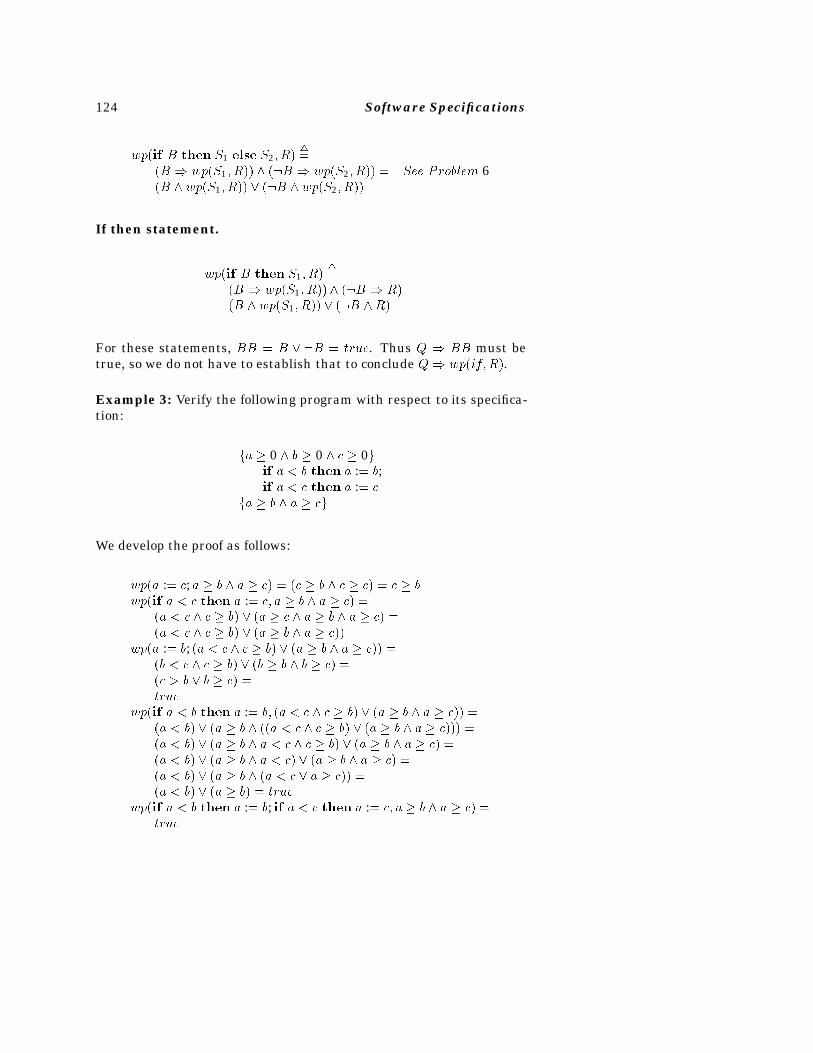
124 Software Specifications
wp�if B then S1 else S2� R���
�B wp�S1� R�� ��B wp�S2� R�� � See Problem 6�B wp�S1� R�� � ��B wp�S2� R��
If then statement.
wp�if B then S1� R���
�B wp�S1� R�� ��B R� ��B wp�S1� R�� � ��B R�
For these statements, BB � B � �B � true. Thus Q BB must betrue, so we do not have to establish that to conclude Q wp�if� R�.
Example 3: Verify the following program with respect to its specifica-tion:
fa � 0 b � 0 c � 0gif a � b then a :� b;if a � c then a :� c
fa � b a � cg
We develop the proof as follows:
wp�a :� c; a � b a � c� � �c � b c � c� � c � bwp�if a � c then a :� c� a � b a � c� �
�a � c c � b� � �a � c a � b a � c� ��a � c c � b� � �a � b a � c��
wp�a :� b; �a � c c � b� � �a � b a � c�� ��b � c c � b� � �b � b b � c� ��c � b � b � c� �true
wp�if a � b then a :� b� �a � c c � b� � �a � b a � c�� ��a � b� � �a � b ��a � c c � b� � �a � b a � c��� ��a � b� � �a � b a � c c � b� � �a � b a � c� ��a � b� � �a � b a � c� � �a � b a � c� ��a � b� � �a � b �a � c � a � c�� ��a � b� � �a � b� � true
wp�if a � b then a :� b; if a � c then a :� c� a � b a � c� �true
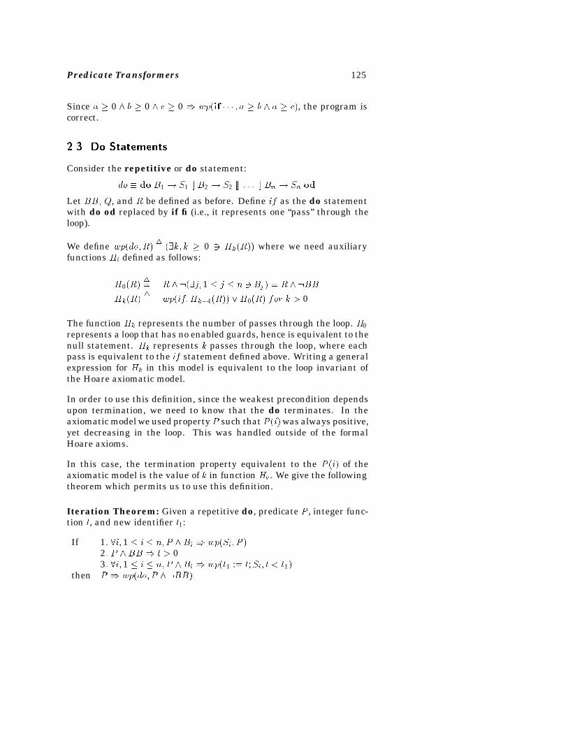
Predicate Transformers 125
Since a � 0 b � 0 c � 0 wp�if � � � � a � b a � c�, the program iscorrect.
���� Do Statements
Consider the repetitive or do statement:
do � do B1 � S1 �� B2 � S2 �� � � � �� Bn � Sn od
Let BB� Q, and R be defined as before. Define if as the do statementwith do od replaced by if fi (i.e., it represents one “pass” through theloop).
We define wp�do�R��� ��k� k � 0 � Hk�R�� where we need auxiliary
functions Hi defined as follows:
H0�R��� R ���j� 1 � j � n � Bj� � R �BB
Hk�R��� wp�if�Hk�1�R�� �H0�R� for k � 0
The function Hk represents the number of passes through the loop. H0represents a loop that has no enabled guards, hence is equivalent to thenull statement. Hk represents k passes through the loop, where eachpass is equivalent to the if statement defined above. Writing a generalexpression for Hk in this model is equivalent to the loop invariant ofthe Hoare axiomatic model.
In order to use this definition, since the weakest precondition dependsupon termination, we need to know that the do terminates. In theaxiomatic model we used property P such that P �i� was always positive,yet decreasing in the loop. This was handled outside of the formalHoare axioms.
In this case, the termination property equivalent to the P �i� of theaxiomatic model is the value of k in function Hk. We give the followingtheorem which permits us to use this definition.
Iteration Theorem: Given a repetitive do, predicate P , integer func-tion t, and new identifier t1:
If 1� �i� 1 � i � n� P Bi wp�Si� P �2� P BB t � 03� �i� 1 � i � n� P Bi wp�t1 :� t;Si� t � t1�
then P wp�do� P �BB�
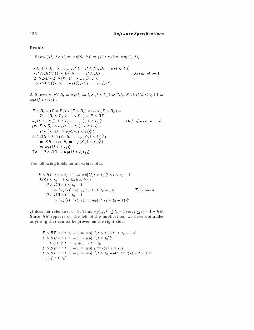
126 Software Specifications
Proof:
1. Show ��i� P Bi wp�Si� P �� �P BB wp�if� P ��.
��i� P Bi wp�Si� P �� � P ��i� Bi wp�Si� P ���P B1� � �P B2� � � � � � P BB Assumption 1P BB P ��i� Bi wp�Si� P �� BB ��i� Bi wp�Si� P �� � wp�if� P �
2. Show ��i� PBi wp�t1 :� t;Si� t � t1�� ��t0� PBBt � t0�1 wp�if� t � t0��.
P Bi � �P B1� � �P B2� � � � � � �P Bn� �P �B1 �B2 � � � � �Bn� � P BB
wp�t1 :� t;Si� t � t1� � wp�Si� t � t1�t1t Def of assignment
��i� P Bi wp�t1 :� t;Si� t � t1�� �P ��i� Bi wp�Si� t � t1�
t1t �
P BB P ��i� Bi wp�Si� t � t1�t1t �
BB ��i� Bi wp�Si� t � t1�t1t �
wp�if� t � t1�t1t
Thus P BB wp�if� t � t1�t1t
The following holds for all values of t0:
P BB t � t0 � 1 wp�if� t � t1�t1t t � t0 � 1
Add t � t0 � 1 to both sides :P BB t � t0 � 1
�wp�if� t � t1�t1t t1 � t0 � 1�t1
t Text subst�P BB t � t0 � 1
�wp�if� t � t1�t1t wp�if� t1 � t0 � 1��t1
t
if does not refer to t1 or t0. Thus wp�if� t1 � t0 � 1� � t1 � t0 � 1 BB.Since BB appears on the left of the implication, we have not addedanything that cannot be proven on the right side.
P BB t � t0 � 1 wp�if� t � t1 t1 � t0 � 1�t1t
P BB t � t0 � 1 wp�if� t � t0�t0t
t � t1 t1 � t0 � 1 t � t0P BB t � t0 � 1 wp�t1 :� t; if� t � t0�P BB t � t0 � 1 wp�if� t � t0�wp�t1 :� t; if� t � t0� �wp�if� t � t0�
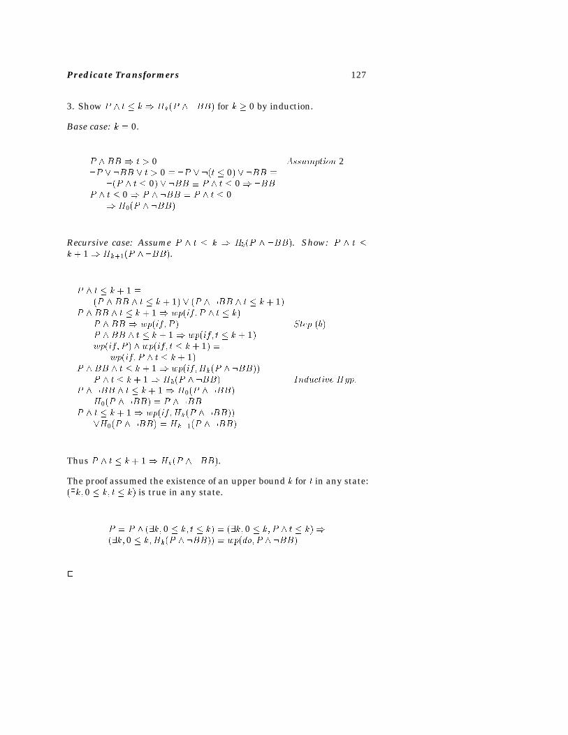
Predicate Transformers 127
3. Show P t � k Hk�P �BB� for k � 0 by induction.
Base case: k � 0.
P BB t � 0 Assumption 2�P � �BB � t � 0 � �P � ��t � 0� � �BB �
��P t � 0� � �BB � P t � 0 �BBP t � 0 P �BB � P t � 0
H0�P �BB�
Recursive case: Assume P t � k Hk�P �BB�. Show: P t �k � 1 Hk�1�P �BB�.
P t � k � 1 ��P BB t � k � 1� � �P �BB t � k � 1�
P BB t � k � 1 wp�if� P t � k�P BB wp�if� P � Step �b�P BB t � k � 1 wp�if� t � k � 1�wp�if� P � wp�if� t � k � 1� �
wp�if� P t � k � 1�P BB t � k � 1 wp�if�Hk�P �BB��
P t � k � 1 Hk�P �BB� Inductive Hyp�P �BB t � k � 1 H0�P �BB�
H0�P �BB� � P �BBP t � k � 1 wp�if�Hk�P �BB��
�H0�P �BB� � Hk�1�P �BB�
Thus P t � k � 1 Hk�P �BB�.
The proof assumed the existence of an upper bound k for t in any state:��k� 0 � k� t � k� is true in any state.
P � P ��k� 0 � k� t � k� � ��k� 0 � k� P t � k���k� 0 � k�Hk�P �BB�� � wp�do� P �BB�
�
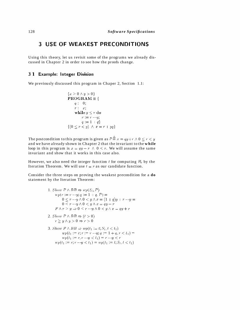
128 Software Specifications
�� USE OF WEAKEST PRECONDITIONS
Using this theory, let us revisit some of the programs we already dis-cussed in Chapter 2 in order to see how the proofs change.
���� Example� Integer Division
We previously discussed this program in Chaper 2, Section 1.1:
fx � 0 y � 0gPROGRAM � f
q :� 0;r :� x;while y � r do
r :� r � y;q :� 1 � qg
f�0 � r � y� x � r � yqg
The postcondition to this program is given asP�� x � qy�r 0 � r � y
and we have already shown in Chapter 2 that the invariant to the whileloop in this program is x � qy � r 0 � r. We will assume the sameinvariant and show that it works in this case also.
However, we also need the integer function t for computing Hk by theIteration Theorem. We will use t � r as our candidate function.
Consider the three steps on proving the weakest precondition for a dostatement by the Iteration Theorem:
1� Show P BB wp�Si� P �wp�r :� r � y; q :� 1 � q� P � �
0 � r � y 0 � y x � �1 � q�y � r � y �0 � r � y 0 � y x � qy � r
P r � y 0 � r � y 0 � y x � qy � r
2� Show P BB �t � 0�r � y y � 0 r � 0
3� Show P BB wp�t1 :� t;Si� t � t1�wp�t1 :� r; r :� r � y; q :� 1 � q� r � t1� �wp�t1 :� r� r� y � t1� � r � y � r
wp�t1 :� r; r� y � t1� � wp�t1 :� t;Si� t � t1�
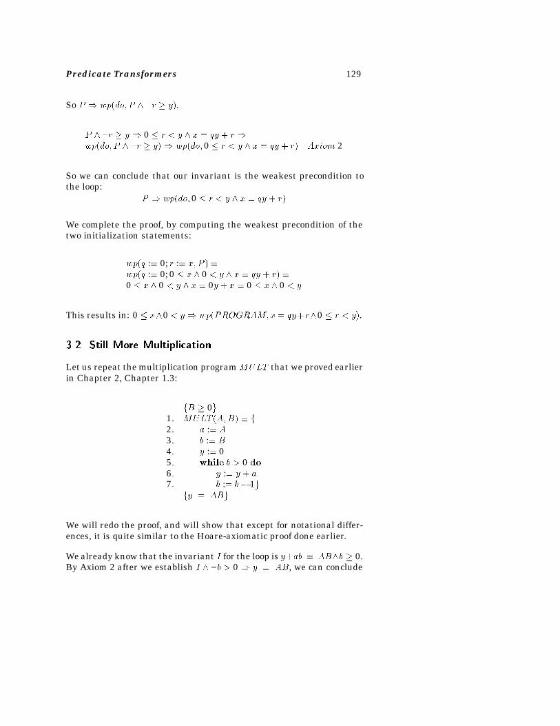
Predicate Transformers 129
So P wp�do� P �r � y�.
P �r � y 0 � r � y x � qy � rwp�do� P �r � y� wp�do� 0 � r � y x � qy � r� Axiom 2
So we can conclude that our invariant is the weakest precondition tothe loop:
P wp�do� 0 � r � y x � qy � r�
We complete the proof, by computing the weakest precondition of thetwo initialization statements:
wp�q :� 0; r :� x� P � �wp�q :� 0; 0 � x 0 � y x � qy � r� �0 � x 0 � y x � 0y � x � 0 � x 0 � y
This results in: 0 � x0 � y wp�PROGRAM�x� qy�r0 � r � y�.
���� Still More Multiplication
Let us repeat the multiplication programMULT that we proved earlierin Chapter 2, Chapter 1.3:
fB � 0g1� MULT �A�B� � f2� a :� A3� b :� B4� y :� 05� while b � 0 do6� y :� y � a7� b :� b� 1g
fy � ABg
We will redo the proof, and will show that except for notational differ-ences, it is quite similar to the Hoare-axiomatic proof done earlier.
We already know that the invariant I for the loop is y�ab � ABb � 0.By Axiom 2 after we establish I �b � 0 y � AB, we can conclude
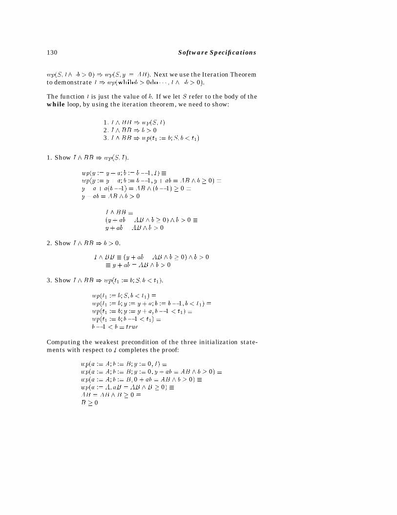
130 Software Specifications
wp�S� I�b � 0� wp�S� y � AB�. Next we use the Iteration Theoremto demonstrate I wp�whileb � 0do � � � � I �b � 0�.
The function t is just the value of b. If we let S refer to the body of thewhile loop, by using the iteration theorem, we need to show:
1� I BB wp�S� I�2� I BB b � 03� I BB wp�t1 :� b;S� b � t1�
1. Show I BB wp�S� I�.
wp�y :� y � a; b :� b� 1� I� �wp�y :� y � a; b :� b� 1� y � ab � AB b � 0� �y � a� a�b� 1� � AB �b� 1� � 0 �y � ab � AB b � 0
I BB ��y � ab � AB b � 0� b � 0 �y � ab � AB b � 0
2. Show I BB b � 0.
I BB � �y � ab � AB b � 0� b � 0� y � ab � AB b � 0
3. Show I BB wp�t1 :� b;S� b � t1�.
wp�t1 :� b;S� b � t1� �wp�t1 :� b; y :� y � a; b :� b� 1� b � t1� �wp�t1 :� b; y :� y � a� b� 1 � t1� �wp�t1 :� b; b� 1 � t1� �b� 1 � b � true
Computing the weakest precondition of the three initialization state-ments with respect to I completes the proof:
wp�a :� A; b :� B; y :� 0� I� �wp�a :� A; b :� B; y :� 0� y � ab � AB b � 0� �wp�a :� A; b :� B� 0 � ab � AB b � 0� �wp�a :� A� aB � AB B � 0� �AB � AB B � 0 �B � 0
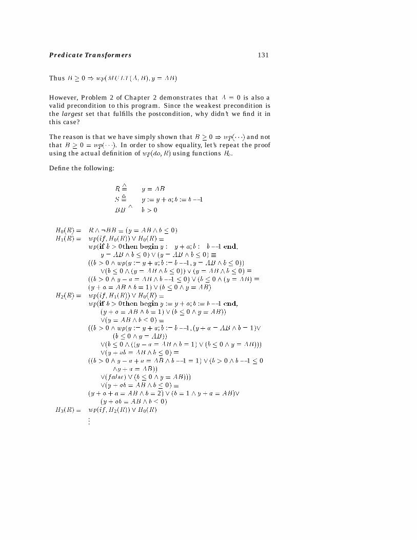
Predicate Transformers 131
Thus B � 0 wp�MULT �A�B�� y � AB�
However, Problem 2 of Chapter 2 demonstrates that A � 0 is also avalid precondition to this program. Since the weakest precondition isthe largest set that fulfills the postcondition, why didn’t we find it inthis case?
The reason is that we have simply shown that B � 0 wp�� � �� and notthat B � 0 � wp�� � ��. In order to show equality, let’s repeat the proofusing the actual definition of wp�do�R� using functions Hk.
Define the following:
R�� y � AB
S�� y :� y � a; b :� b� 1
BB�� b � 0
H0�R� � R �BB � �y � AB b � 0�H1�R� � wp�if�H0�R�� �H0�R� �
wp�if b � 0then begin y :� y � a; b :� b� 1 end�y � AB b � 0� � �y � AB b � 0� �
��b � 0 wp�y :� y � a; b :� b� 1� y � AB b � 0����b � 0 �y � AB b � 0�� � �y � AB b � 0� �
��b � 0 y � a � AB b � 1 � 0� � �b � 0 �y � AB� ��y � a � AB b � 1� � �b � 0 y � AB�
H2�R� � wp�if�H1�R�� �H0�R� �wp�if b � 0then begin y :� y � a; b :� b� 1 end�
�y � a � AB b � 1� � �b � 0 y � AB����y � AB b � 0� �
��b � 0 wp�y :� y � a; b :� b� 1� �y � a � AB b � 1���b � 0 y � AB��
��b � 0 ��y � a � AB b � 1� � �b � 0 y � AB�����y � ab � AB b � 0� �
��b � 0 y � a � a � AB b� 1 � 1� � �b � 0 b� 1 � 0y � a � AB��
��false� � �b � 0 y � AB�����y � ab � AB b � 0� �
�y � a� a � AB b � 2� � �b � 1 y � a � AB���y � ab � AB b � 0�
H3�R� � wp�if�H2�R�� �H0�R�...
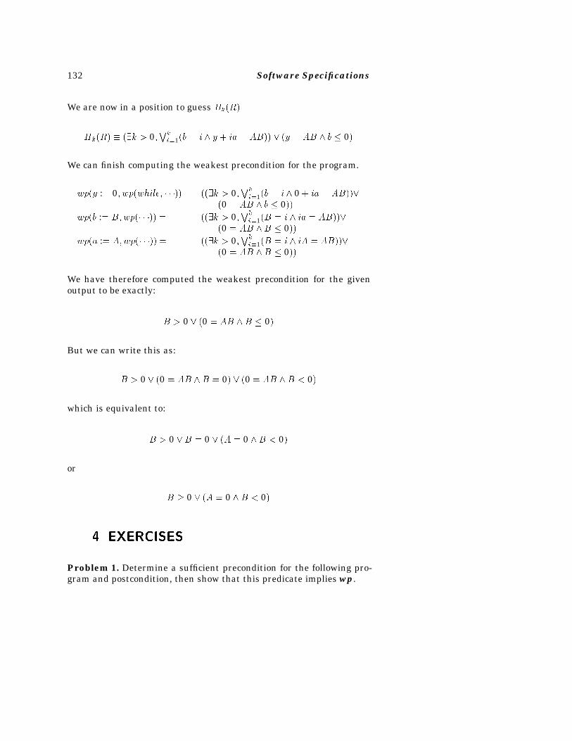
132 Software Specifications
We are now in a position to guess Hk�R�
Hk�R� � ��k � 0�Wki�1�b � i y � ia � AB�� � �y � AB b � 0�
We can finish computing the weakest precondition for the program.
wp�y :� 0� wp�while� � � ��� � ���k � 0�Wki�1�b � i 0 � ia � AB���
�0 � AB b � 0��wp�b :� B�wp�� � ��� � ���k � 0�
Wki�1�B � i ia � AB���
�0 � AB B � 0��wp�a :� A�wp�� � ��� � ���k � 0�
Wki�1�B � i iA � AB���
�0 � AB B � 0��
We have therefore computed the weakest precondition for the givenoutput to be exactly:
B � 0 � �0 � AB B � 0�
But we can write this as:
B � 0 � �0 � AB B � 0� � �0 � AB B � 0�
which is equivalent to:
B � 0 �B � 0 � �A � 0 B � 0�
or
B � 0 � �A � 0 B � 0�
�� EXERCISES
Problem 1. Determine a sufficient precondition for the following pro-gram and postcondition, then show that this predicate implies wp.
Predicate Transformers 133
i :� 1m :� a�1�while i �� 100 do
if m � a�i� 1� thenm :� a�i� 1�i :� i� 1
f��j � 1 � j � 100�m � a�j�� ��k � 1 � k � 100�m � a�k��g
Problem 2. Determine a sufficient precondition for the following pro-gram and postcondition, then show that this predicate implies wp.
k :� awhile k � b do
k :� k � 1x�k � 1� :� x�k�
fa � k � b ��i � a � i � b� x�i� ��x �i� 1��g
Give the precondition if the postcondition were written as:
fa � k � b ��i � a � i � b� x�i� � x�i� 1��g
Problem 3. Using predicate transformers verify the following pro-gram:
fn � 0gi :� 1p :� 1while i �� n do
if b�i� �� b�i� p�then i :� i � 1else i :� i� 1; p :� p� 1
f��k � 0 � k � n � p� b�k� � b�k� p� 1����k � 0 � k � n� p� 1� b�k� �� b�k� p��g
Problem 4. Using the method of predicate transformers, demonstratethe correctness of the following array reversal program:
134 Software Specifications
fi � 1 n � 0gwhile i � n2 do
z :� a�i�a�i� :� a�n� i� 1�a�n� i � 1� :� zi :� i� 1
f�j � 1 � j � n� a�j� ��a �n� j � 1�g
Problem 5. Consider the following program:
fi � 1gwhile i � n do
a�i� 1� :� a�i� � a�i� 1�i :� i � 1
f�j � 1 � j � n� a�j� �Pj
k�1�a �k�g
Verify the total (strong) correctness of the program with respect to thegiven pre- and postconditions using the method of predicate transform-ers.
Problem 6. From the definition of the weakest precondition for thetraditional if then else statement, show the following is true:
�B wp�S1� R�� ��B wp�S2� R�� ��B wp�S1� R��� ��B wp�S2� R��
�� SUGGESTED READINGS
� E. W. Dijkstra, “Guarded commands, nondeterminacy and formalderivation of programs,” Communications of the ACM, Vol. 18, No.8, 1975, pp. 453-458.
� S. K. Basu and R. T. Yeh, “Strong Verification of Programs,” IEEETransactions on Software Engineering, Vol. 1, No. 3, 1975, pp. 339-346.
� E. W. Dijkstra, “A Discipline of Programming,” Prentice-Hall, Engle-wood Cliffs, NJ, 1976.
Predicate Transformers 135
� D. Gries, The Science of Programming, Springer-Verlag, New York,1981.

136 Software Specifications
Chapter 5
Algebraic Specifications
Up to this point, we have dealt primarily with integer data types inthe application programs. But to continue to do so would be veryrestrictive to programmers. In fact, not only do we want to find waysto reason about programs having many different primitive types (suchas strings, characters, or floating point numbers), but we want to buildan inference system that allows programs to be verified even when theapplication programmer is free to enrich the environment with newand special purpose types.
�� MORE ABOUT DATA ABSTRACTIONS
Being able to add new data types on a program by program basis is apowerful capability. This concept, which evolved in the 1970s, is knownas data abstraction (or, looked at another way, encapsulation), and it isa major “divide and conquer” technique available to help programmerskeep development costs down. The idea is to identify commonly usedactivities or information, and then, abstracting from the situation, ex-plicitly describe that information structure in a concise and centralizedway. Once the structure has been isolated, then one programmer cango off and implement the data-handling routines, another can work onthe application program using the data, and both will be assured thatthe union of their efforts will function as intended.
137
138 Software Specifications
We previous discussed data abstractions in Chapter 3. Here we extendthe concept and discuss why we have this concept of “type” in thefirst place. Associating a “type” name with some piece of data is adeclaration by the programmer concerning how that data is intendedto be used. When the only thing we can declare about a datum is thatit is an integer or string, then there is still much room for misuse ofthat information. However, when a designer abstracts some collectionof desirable properties and declares this collection to be a new “type,”then it is easier to infer more about the intended usage of the data. Theprogrammer can say stronger things about the program components.In general, the way a designer will perform this abstraction activitywill vary from methodology to methodology, and this is (currently) wellbeyond what we study in this course. However, once a new type hasbeen defined it is essential that we be able to
1. verify that implementations of the new type preserve properties thatcharacterize it, and
2. reason about application programs that use the new type.
For our purposes, a data type consists a set of values (its domain)and a set of operations on the domain. Defining the domain is usuallystraightforward: Small, finite domains can be enumerated. Others canbe defined constructively, by first identifying a small number of baseelements, and then describing how to generate the remaining elementsof the domain. For instance, the string domain can be constructed bysaying:
� A single letter is a string.
� Any string followed by a single letter is a string.
� Nothing else is a string.
This third assertion helps us get a bound on what can be a string.
Once the domain is specified, we are faced with describing the oper-ations on it. The first step is to enumerate these operators’ names,and identify in some way what types of values they both operate on(completely) and also return. This step is referred to as prescribing thesyntax, and the way we give syntax is usually dependent on the waywe intend to describe the operator’s functionality (or semantics).
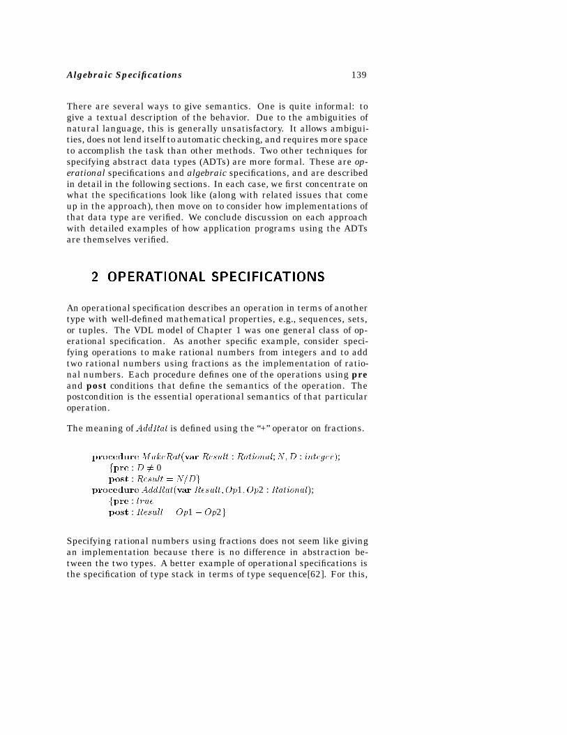
Algebraic Specifications 139
There are several ways to give semantics. One is quite informal: togive a textual description of the behavior. Due to the ambiguities ofnatural language, this is generally unsatisfactory. It allows ambigui-ties, does not lend itself to automatic checking, and requires more spaceto accomplish the task than other methods. Two other techniques forspecifying abstract data types (ADTs) are more formal. These are op-erational specifications and algebraic specifications, and are describedin detail in the following sections. In each case, we first concentrate onwhat the specifications look like (along with related issues that comeup in the approach), then move on to consider how implementations ofthat data type are verified. We conclude discussion on each approachwith detailed examples of how application programs using the ADTsare themselves verified.
�� OPERATIONAL SPECIFICATIONS
An operational specification describes an operation in terms of anothertype with well-defined mathematical properties, e.g., sequences, sets,or tuples. The VDL model of Chapter 1 was one general class of op-erational specification. As another specific example, consider speci-fying operations to make rational numbers from integers and to addtwo rational numbers using fractions as the implementation of ratio-nal numbers. Each procedure defines one of the operations using preand post conditions that define the semantics of the operation. Thepostcondition is the essential operational semantics of that particularoperation.
The meaning of AddRat is defined using the “+” operator on fractions.
procedureMakeRat�var Result : Rational;N�D : integer�;fpre : D �� 0post : Result � NDg
procedure AddRat�var Result� Op1� Op2 : Rational�;fpre : truepost : Result � Op1 � Op2g
Specifying rational numbers using fractions does not seem like givingan implementation because there is no difference in abstraction be-tween the two types. A better example of operational specifications isthe specification of type stack in terms of type sequence[62]. For this,
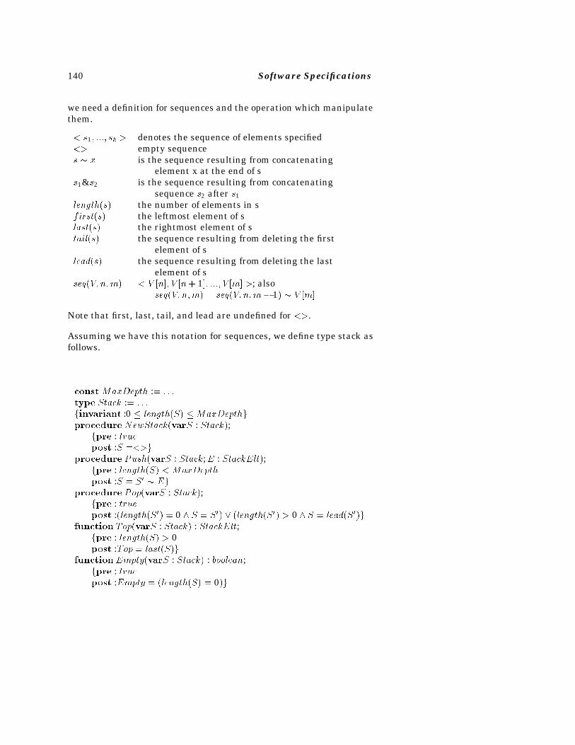
140 Software Specifications
we need a definition for sequences and the operation which manipulatethem.
� s1� ���� sk � denotes the sequence of elements specified�� empty sequences � x is the sequence resulting from concatenating
element x at the end of ss1&s2 is the sequence resulting from concatenating
sequence s2 after s1length�s� the number of elements in sfirst�s� the leftmost element of slast�s� the rightmost element of stail�s� the sequence resulting from deleting the first
element of slead�s� the sequence resulting from deleting the last
element of sseq�V� n�m� � V �n�� V �n� 1�� ���� V �m� �; also
seq�V� n�m� � seq�V� n�m � 1� � V �m�
Note that first, last, tail, and lead are undefined for ��.
Assuming we have this notation for sequences, we define type stack asfollows.
constMaxDepth :� � � �type Stack :� � � �finvariant :0 � length�S� �MaxDepthgprocedure NewStack�varS : Stack�;
fpre : truepost :S ���g
procedure Push�varS : Stack;E : StackElt�;fpre : length�S� � MaxDepthpost :S � S� � Eg
procedure Pop�varS : Stack�;fpre : truepost :�length�S�� � 0 S � S�� � �length�S�� � 0 S � lead�S��g
function Top�varS : Stack� : StackElt;fpre : length�S� � 0post :Top � last�S�g
functionEmpty�varS : Stack� : boolean;fpre : truepost :Empty � �length�S� � 0�g
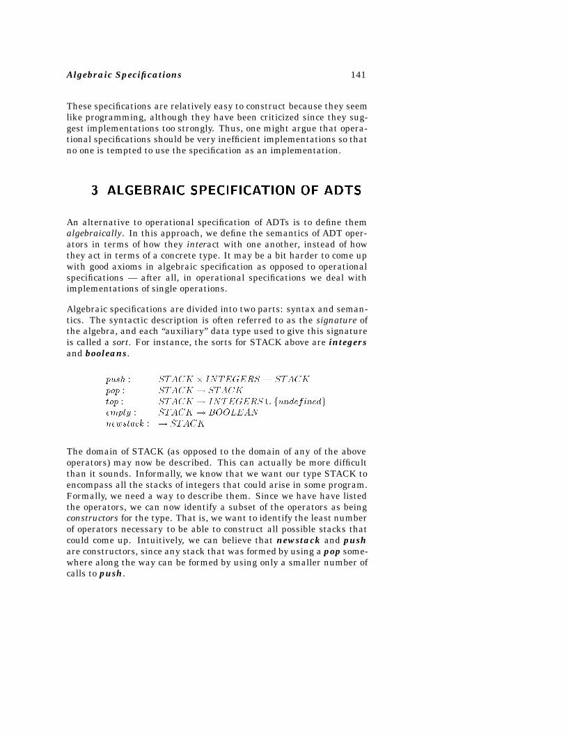
Algebraic Specifications 141
These specifications are relatively easy to construct because they seemlike programming, although they have been criticized since they sug-gest implementations too strongly. Thus, one might argue that opera-tional specifications should be very inefficient implementations so thatno one is tempted to use the specification as an implementation.
�� ALGEBRAIC SPECIFICATION OF ADTS
An alternative to operational specification of ADTs is to define themalgebraically. In this approach, we define the semantics of ADT oper-ators in terms of how they interact with one another, instead of howthey act in terms of a concrete type. It may be a bit harder to come upwith good axioms in algebraic specification as opposed to operationalspecifications — after all, in operational specifications we deal withimplementations of single operations.
Algebraic specifications are divided into two parts: syntax and seman-tics. The syntactic description is often referred to as the signature ofthe algebra, and each “auxiliary” data type used to give this signatureis called a sort. For instance, the sorts for STACK above are integersand booleans.
push : STACK � INTEGERS � STACKpop : STACK � STACKtop : STACK � INTEGERS � fundefinedgempty : STACK � BOOLEANnewstack : � STACK
The domain of STACK (as opposed to the domain of any of the aboveoperators) may now be described. This can actually be more difficultthan it sounds. Informally, we know that we want our type STACK toencompass all the stacks of integers that could arise in some program.Formally, we need a way to describe them. Since we have have listedthe operators, we can now identify a subset of the operators as beingconstructors for the type. That is, we want to identify the least numberof operators necessary to be able to construct all possible stacks thatcould come up. Intuitively, we can believe that newstack and pushare constructors, since any stack that was formed by using a pop some-where along the way can be formed by using only a smaller number ofcalls to push.
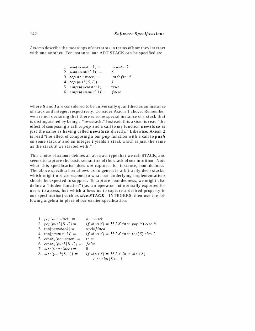
142 Software Specifications
Axioms describe the meanings of operators in terms of how they interactwith one another. For instance, our ADT STACK can be specified as:
1� pop�newstack� � newstack2� pop�push�S� I�� � S3� top�newstack� � undefined4� top�push�S� I�� � I5� empty�newstack� � true6� empty�push�S� I�� � false
where S and I are considered to be universally quantified as an instanceof stack and integer, respectively. Consider Axiom 1 above: Rememberwe are not declaring that there is some special instance of a stack thatis distinguished by being a “newstack.” Instead, this axiom is read “theeffect of composing a call to pop and a call to my function newstack isjust the same as having called newstack directly.” Likewise, Axiom 2is read “the effect of composing a our pop function with a call to pushon some stack S and an integer I yields a stack which is just the sameas the stack S we started with.”
This choice of axioms defines an abstract type that we call STACK, andseems to capture the basic semantics of the stack of our intuition. Notewhat this specification does not capture, for instance, boundedness.The above specification allows us to generate arbitrarily deep stacks,which might not correspond to what our underlying implementationsshould be expected to support. To capture boundedness, we might alsodefine a “hidden function” (i.e. an operator not normally exported forusers to access, but which allows us to capture a desired property inour specification) such as size:STACK�INTEGERS, then use the fol-lowing algebra in place of our earlier specification:
1� pop�newstack� � newstack2� pop�push�S� I�� � if size�S� � MAX then pop�S� else S3� top�newstack� � undefined4� top�push�S� I�� � if size�S� � MAX then top�S� else I5� empty�newstack� � true6� empty�push�S� I�� � false7� size�newstack� � 08� size�push�S� I�� � if size�S� � MAX then size�S�
else size�S� � 1
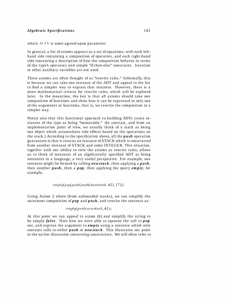
Algebraic Specifications 143
where MAX is some agreed-upon parameter.
In general, a list of axioms appears as a set of equations, with each left-hand side containing a composition of operators, and each right-handside containing a description of how the composition behaves in termsof the type’s operators and simple “if-then-else” constructs. Iterationor other auxiliary variables are not used.
These axioms are often thought of as “rewrite rules.” Informally, thisis because we can take one instance of the ADT and appeal to the listto find a simpler way to express that instance. However, there is amore mathematical criteria for rewrite rules, which will be exploredlater. In the meantime, the key is that all axioms should take onecomposition of functions and show how it can be expressed in only oneof the arguments or functions, that is, we rewrite the composition in asimpler way.
Notice also that this functional approach to building ADTs treats in-stances of the type as being “immutable.” (In contrast, and from animplementation point of view, we usually think of a stack as beingone object which accumulates side effects based on the operations onthe stack.) According to the specification above, all the push operationguarantees is that it returns an instance of STACK which is constructedfrom another instance of STACK and some INTEGER. This situation,together with our ability to view the axioms as rewrite rules, allowsus to think of instances of an algebraically specified ADT as beingsentences in a language, a very useful perspective. For example, onesentence might be formed by calling newstack, then applying a push,then another push, then a pop, then applying the query empty, forexample,
empty�pop�push�push�newstack� 42�� 17���
Using Axiom 2 above (from unbounded stacks), we can simplify theoutermost composition of pop and push, and rewrite the sentence as:
empty�push�newstack� 42��
At this point we can appeal to axiom (6) and simplify the string tobe simply false. Note how we were able to squeeze the call to popout, and express the argument to empty using a sentence which onlycontains calls to either push or newstack. This illustrates our pointin the earlier discussion concerning constructors. We will often refer to
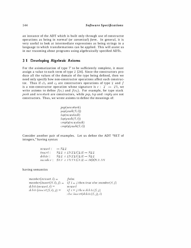
144 Software Specifications
an instance of the ADT which is built only through use of constructoroperations as being in normal (or canonical) form. In general, it isvery useful to look at intermediate expressions as being strings in alanguage to which transformations can be applied. This will assist usin our reasoning about programs using algebraically specified ADTs.
���� Developing Algebraic Axioms
For the axiomatization of type T to be sufficiently complete, it mustassign a value to each term of type T [24]. Since the constructors pro-duce all the values of the domain of the type being defined, then weneed only specify how non-constructor operations affect each construc-tor. Thus if c11 and c2 are constructors operations of type T and fis a non-constructor operation whose signature is r : T � T1, wewrite axioms to define f�c1� and f�c2�. For example, for type stackpush and newstack are constructors, while pop, top and empty are notconstructors. Thus, we wrote axioms to define the meanings of:
pop�newstack�pop�push�S� i��top�newstack�top�push�S� i��empty�newstack�empty�push�S� i��
Consider another pair of examples. Let us define the ADT “SET ofintegers,” having syntax
newset : � SETinsert : SET � INTEGER� SETdelete : SET � INTEGER� SETmember : SET � INTEGER� BOOLEAN
having semantics
member�newset� i� � falsemember�insert�S� i�� j� � if i � j then true else member�S� j�delete�newset� i� � newsetdelete�insert�S� i�� j� � if i � j then delete�S� j�
else insert�delete�S� j�� i�
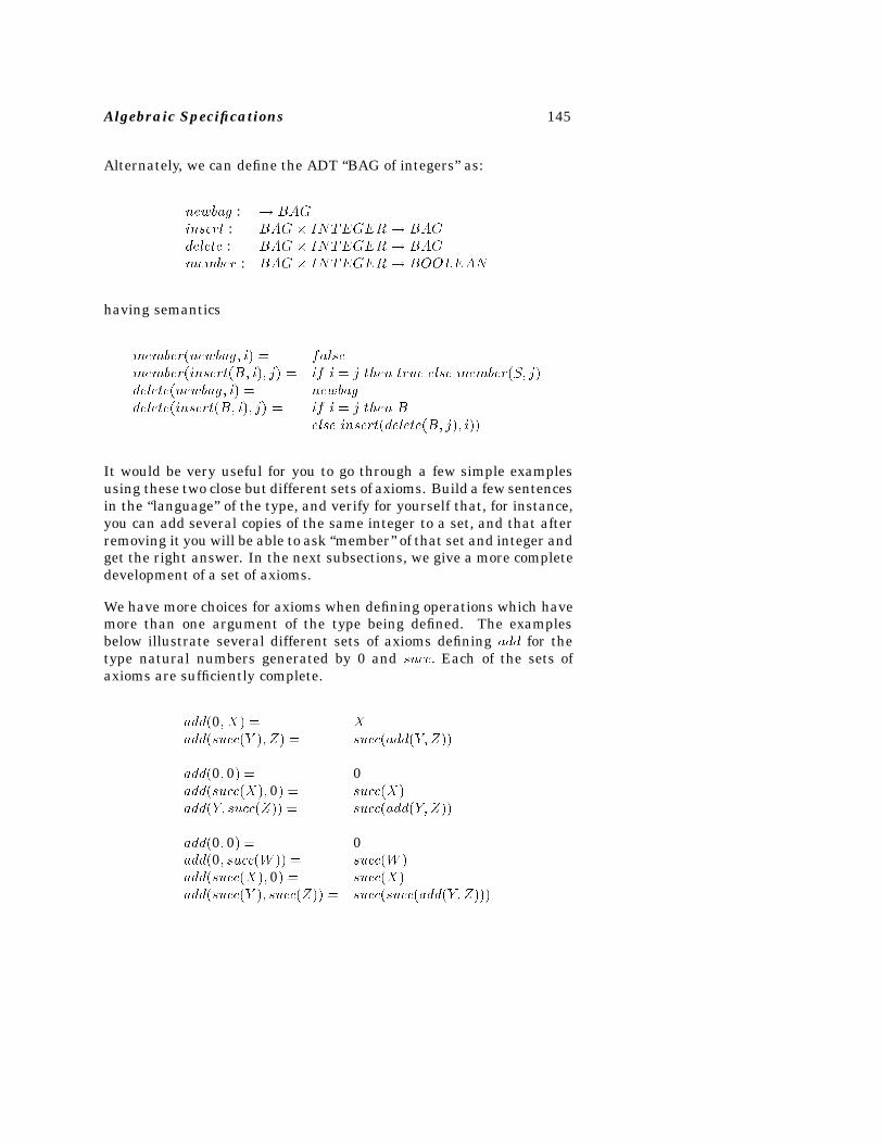
Algebraic Specifications 145
Alternately, we can define the ADT “BAG of integers” as:
newbag : � BAGinsert : BAG � INTEGER� BAGdelete : BAG � INTEGER� BAGmember : BAG � INTEGER� BOOLEAN
having semantics
member�newbag� i� � falsemember�insert�B� i�� j� � if i � j then true else member�S� j�delete�newbag� i� � newbagdelete�insert�B� i�� j� � if i � j then B
else insert�delete�B� j�� i��
It would be very useful for you to go through a few simple examplesusing these two close but different sets of axioms. Build a few sentencesin the “language” of the type, and verify for yourself that, for instance,you can add several copies of the same integer to a set, and that afterremoving it you will be able to ask “member” of that set and integer andget the right answer. In the next subsections, we give a more completedevelopment of a set of axioms.
We have more choices for axioms when defining operations which havemore than one argument of the type being defined. The examplesbelow illustrate several different sets of axioms defining add for thetype natural numbers generated by 0 and succ� Each of the sets ofaxioms are sufficiently complete.
add�0� X� � Xadd�succ�Y �� Z� � succ�add�Y� Z��
add�0� 0� � 0add�succ�X�� 0� � succ�X�add�Y� succ�Z�� � succ�add�Y� Z��
add�0� 0� � 0add�0� succ�W �� � succ�W �add�succ�X�� 0� � succ�X�add�succ�Y �� succ�Z�� � succ�succ�add�Y� Z���
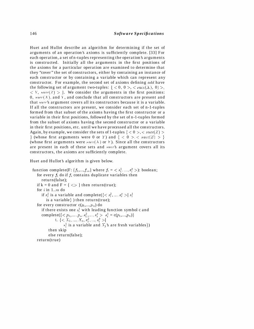
146 Software Specifications
Huet and Hullot describe an algorithm for determining if the set ofarguments of an operation’s axioms is sufficiently complete. [33] Foreach operation, a set of n-tuples representing the operation’s argumentsis constructed. Initially all the arguments in the first positions ofthe axioms for a particular operation are examined to determine thatthey “cover” the set of constructors, either by containing an instance ofeach constructor or by containing a variable which can represent anyconstructor. For example, the second set of axioms defining add havethe following set of argument two-tuples: f � 0� 0 �, � succ�X�� 0� ��� Y� succ�Z� � g. We consider the arguments in the first positions:0� succ�X�� and Y , and conclude that all constructors are present andthat succ’s argument covers all its constructors because it is a variable.If all the constructors are present, we consider each set of n-1-tuplesformed from that subset of the axioms having the first constructor or avariable in their first positions, followed by the set of n-1-tuples formedfrom the subset of axioms having the second constructor or a variablein their first positions, etc. until we have processed all the constructors.Again, by example, we consider the sets of 1-tuples f� 0 ��� succ�Z� �g (whose first arguments were 0 or Y ) and f � 0 ��� succ�Z� � g(whose first arguments were succ�X� or Y ). Since all the constructorsare present in each of these sets and succ’s argument covers all itsconstructors, the axioms are sufficiently complete.
Huet and Hullot’s algorithm is given below.
function complete(F: ff1,...,fmg where fi = � s1i � ���� s
ki �): boolean;
for every fi do if fi contains duplicate variables thenreturn(false);
if k = 0 and F = f �� g then return(true);for i in 1..m do
if s1i is a variable and complete(f� s2i � ���� s
ki �j s
1i
is a variableg ) then return(true);for every constructor c(p1,...,pn) do
if there exists one s1i with leading function symbol c and
complete(f� p1� ���� pn� s2i � ���� s
ki �j s
1i = c(p1,...,pn)g
� f� X1� ���� Xn� s2i � ���� s
ki �j
s1i is a variable and Xj ’s are fresh variablesg)
then skipelse return(false);
return(true)
Algebraic Specifications 147
���� Hints For writing algebraic axioms
The process of writing algebraic specifications is similar to that ofprogramming.1 The main difference is that in programming we areinterested in the efficiency of the solutions, whereas in specifying weare interested in expressing the functionality and nothing else (i.e.,avoid implementation bias). This means that in writing specificationswe want to express only the function to be computed, not the methodof computation. Besides, algebraic specification languages do not havethe concept of side effect (e.g., variable assignment) every time a newvalue is created, so algebraic specifications resemble so-called func-tional programs.
Determine functionality
You should determine the use of the data type, what operations createinstances of the data type, what operations modify instances,2 whatoperations obtain values from the data type, etc. To determine thesefunctions you must think about the uses of the data type. This mightbe hard, especially if this is a “general-purpose” type and you cannotanticipate all its uses.
Write signatures
Once you have decided which is the set of functions, you write thesignatures of them. In this step you can provide a lot of insight on theabstract type if you use appropriate, meaningful names. Note, howeverthat the final word on meaning is not the name: This is the whole pointof using formal specifications.
Choose constructors
Initially all functions that yield the defined type are candidates for con-structors. In principle, you can have them all as constructors, but thatwill introduce many problems both in the consistency of your axiomsand also in the number of axioms (equations) that you have to provide.
1We are indebted to Pablo Straub of the Catholic University of Chile for contributing thispart.
2In the specification no modification is allowed, but modification is expressed by creationof a new instance that is very similar to the original.
148 Software Specifications
Hence you want a “minimal” set of constructors. This set of construc-tors will have at least one function that has no parameter of the typedefined (usually it will be a function with no parameters at all).
If you can figure out how to express the semantics of a function in termsof others, then this function is not a constructor. Besides, the way youexpress the semantics of the function will dictate the axioms you willwrite later.
Sometimes which operations are constructors is evident from the speci-fication; sometimes there are explicit choices to be made. For example,consider a specification for a dequeue, a list with insertion and deletionon both ends. We have two possible sets of constructors: fAddFront,Newg and fAddBack, Newg. Which one to use is a matter of taste, butyou should decide on one of them.
Write axioms
The first part is to determine which axioms you need to write. Con-structors do not need axioms: you will only write axioms for noncon-structors. For each nonconstructor function, you need to cover all casesof the parameters. As a rule of thumb, if there are n constructors youwill need n equations for each nonconstructor.
This rule of thumb is not complete, though, because sometimes thereis more than one parameter of the defined type, so you may need moreaxioms. For example if you are defining a function with 3 parametersof the type defined and you have 2 constructors, you may need 23 � 8equations to cover all constructor combinations. Besides, sometimesyou need to consider nesting of constructors to discriminate differentcases. Fortunately, this rarely occurs in practice, and you will usuallybe able to cover all cases with just a few equations.
Now that you know all cases to consider, you write the left-hand sideof all axioms. There are no general methods to write the right-handside, though. While writing the axioms you will notice that some lefthand sides are meaningless (e.g., extract information from an emptydata structure). From this you define your exceptions.
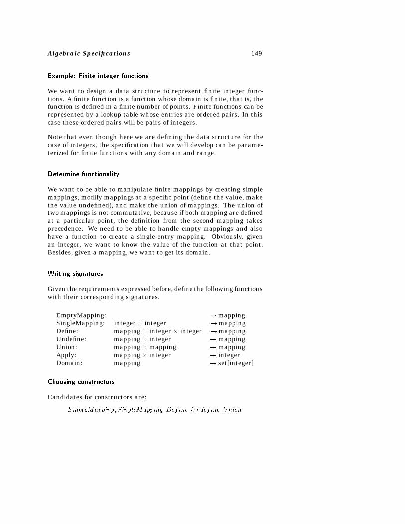
Algebraic Specifications 149
Example� Finite integer functions
We want to design a data structure to represent finite integer func-tions. A finite function is a function whose domain is finite, that is, thefunction is defined in a finite number of points. Finite functions can berepresented by a lookup table whose entries are ordered pairs. In thiscase these ordered pairs will be pairs of integers.
Note that even though here we are defining the data structure for thecase of integers, the specification that we will develop can be parame-terized for finite functions with any domain and range.
Determine functionality
We want to be able to manipulate finite mappings by creating simplemappings, modify mappings at a specific point (define the value, makethe value undefined), and make the union of mappings. The union oftwo mappings is not commutative, because if both mapping are definedat a particular point, the definition from the second mapping takesprecedence. We need to be able to handle empty mappings and alsohave a function to create a single-entry mapping. Obviously, givenan integer, we want to know the value of the function at that point.Besides, given a mapping, we want to get its domain.
Writing signatures
Given the requirements expressed before, define the following functionswith their corresponding signatures.
EmptyMapping: � mappingSingleMapping: integer � integer � mappingDefine: mapping � integer � integer � mappingUndefine: mapping � integer � mappingUnion: mapping � mapping � mappingApply: mapping � integer � integerDomain: mapping � set[integer]
Choosing constructors
Candidates for constructors are:
EmptyMapping� SingleMapping�Define� Undefine� Union
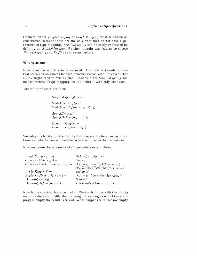
150 Software Specifications
Of them, either EmptyMapping or SingleMapping must be chosen asconstructor, because these are the only ones that do not have a pa-rameter of type mapping. SingleMapping can be easily expressed bydefining an EmptyMapping. Further thought can lead us to chooseEmptyMapping and Define as the constructors.
Writing axioms
First, consider which axioms we need. Our rule of thumb tells usthat we need two axioms for each nonconstructor, with the caveat thatUnion might require four axioms. Besides, since SingleMapping hasno parameters of type mapping, we can define it with only one axiom.
The left-hand sides are then:
SingleMapping�i� v� �
Undefine�Empty� i� �Undefine�Define�m� i1 � v�� i2� �
Apply�Empty� i� �Apply�Define�m� i1 � v�� i2� �
Domain�Empty� �Domain�Define�m� i� v�� �
We delay the left-hand sides for the Union operation because we do notknow yet whether we will be able to do it with two or four equations.
Now we define the semantics of all operations except Union.
SingleMapping�i� v� � Define�Empty� i� v�Undefine�Empty� i� � EmptyUndefine�Define�m� i1 � v�� i2� � if i1 � i2 then Undefine�m� i2�
else Define�Undefine�m� i2�� i1� v�Apply�Empty� i� � unde�ned
Apply�Define�m� i1 � v�� i2� � if i1 � i2 then v else Apply�m� i2�Domain�Empty� � NullSetDomain�Define�m� i� v�� � AddMember�Domain�m�� i�
Now let us consider function Union. Obviously union with the Emptymapping does not modify the mapping. So as long as one of the map-pings is empty the result is trivial. What happens with two nonempty
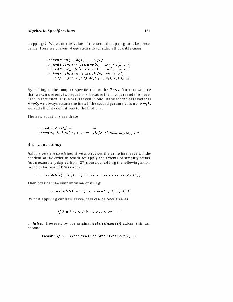
Algebraic Specifications 151
mappings? We want the value of the second mapping to take prece-dence. Here we present 4 equations to consider all possible cases.
Union�Empty�Empty� � EmptyUnion�Define�m� i� v�� Empty� � Define�m� i� v�Union�Empty�Define�m� i� v�� � Define�m� i� v�Union�Define�m1 � i1� v1�� Define�m2 � i2� v2�� �
Define�Union�Define�m1 � i1� v1��m2�� i2� v2�
By looking at the complex specification of the Union function we notethat we can use only two equations, because the first parameter is neverused in recursion: It is always taken in toto. If the second parameter isEmpty we always return the first; if the second parameter is not Emptywe add all of its definitions to the first one.
The new equations are these
Union�m�Empty� � mUnion�m1� Define�m2 � i� v�� � Define�Union�m1 �m2�� i� v�
���� Consistency
Axioms sets are consistent if we always get the same final result, inde-pendent of the order in which we apply the axioms to simplify terms.As an example (adapted from [27]), consider adding the following axiomto the definition of BAGs above:
member�delete�S� i�� j� � if i � j then false else member�S� j�
Then consider the simplification of string:
member�delete�insert�insert�newbag� 3�� 3�� 3�� 3�
By first applying our new axiom, this can be rewritten as
if 3 � 3 then false else member�� � ��
or false. However, by our original delete(insert()) axiom, this canbecome
member�if 3 � 3 then insert�newbag� 3� else delete�� � ��
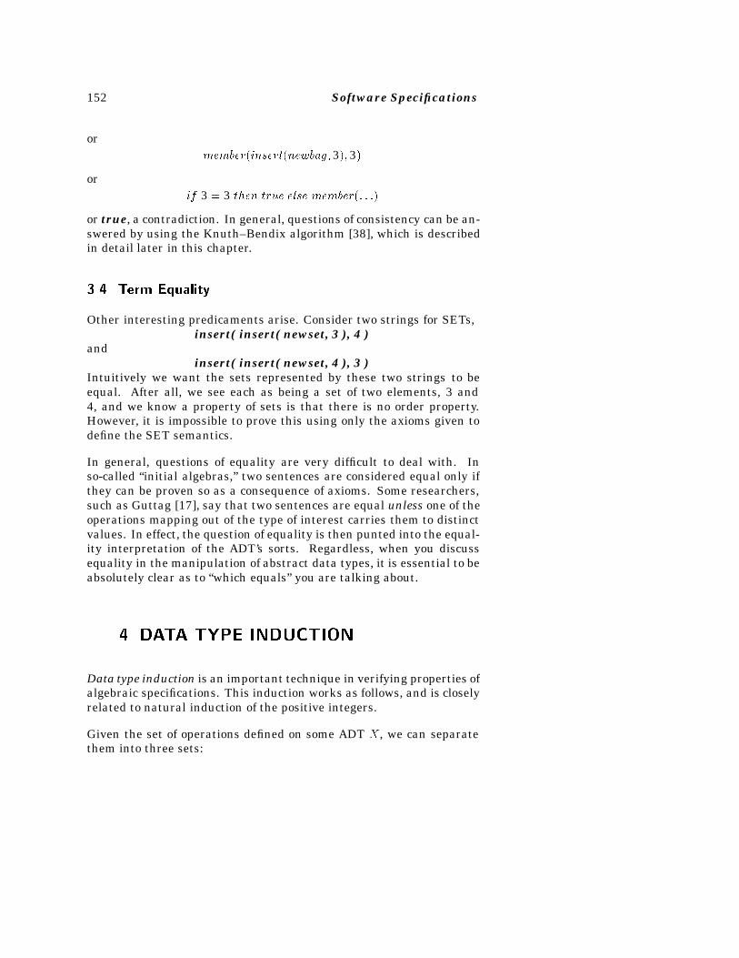
152 Software Specifications
ormember�insert�newbag� 3�� 3�
orif 3 � 3 then true else member�� � ��
or true, a contradiction. In general, questions of consistency can be an-swered by using the Knuth–Bendix algorithm [38], which is describedin detail later in this chapter.
���� Term Equality
Other interesting predicaments arise. Consider two strings for SETs,insert( insert( newset, 3 ), 4 )
andinsert( insert( newset, 4 ), 3 )
Intuitively we want the sets represented by these two strings to beequal. After all, we see each as being a set of two elements, 3 and4, and we know a property of sets is that there is no order property.However, it is impossible to prove this using only the axioms given todefine the SET semantics.
In general, questions of equality are very difficult to deal with. Inso-called “initial algebras,” two sentences are considered equal only ifthey can be proven so as a consequence of axioms. Some researchers,such as Guttag [17], say that two sentences are equal unless one of theoperations mapping out of the type of interest carries them to distinctvalues. In effect, the question of equality is then punted into the equal-ity interpretation of the ADT’s sorts. Regardless, when you discussequality in the manipulation of abstract data types, it is essential to beabsolutely clear as to “which equals” you are talking about.
�� DATA TYPE INDUCTION
Data type induction is an important technique in verifying properties ofalgebraic specifications. This induction works as follows, and is closelyrelated to natural induction of the positive integers.
Given the set of operations defined on some ADT X, we can separatethem into three sets:
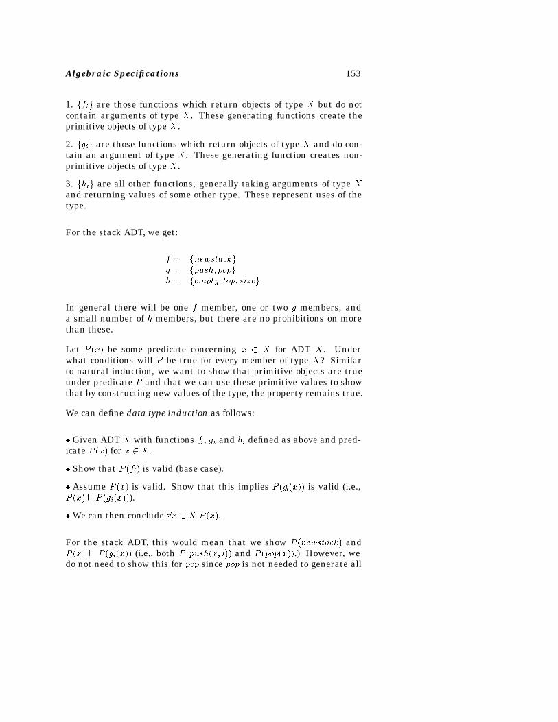
Algebraic Specifications 153
1. ffig are those functions which return objects of type X but do notcontain arguments of type X. These generating functions create theprimitive objects of type X.
2. fgig are those functions which return objects of type X and do con-tain an argument of type X. These generating function creates non-primitive objects of type X.
3. fhig are all other functions, generally taking arguments of type Xand returning values of some other type. These represent uses of thetype.
For the stack ADT, we get:
f � fnewstackgg � fpush� popgh � fempty� top� sizeg
In general there will be one f member, one or two g members, anda small number of h members, but there are no prohibitions on morethan these.
Let P �x� be some predicate concerning x � X for ADT X. Underwhat conditions will P be true for every member of type X? Similarto natural induction, we want to show that primitive objects are trueunder predicate P and that we can use these primitive values to showthat by constructing new values of the type, the property remains true.
We can define data type induction as follows:
� Given ADT X with functions fi, gi and hi defined as above and pred-icate P �x� for x � X.
� Show that P �fi� is valid (base case).
� Assume P �x� is valid. Show that this implies P �gi�x�� is valid (i.e.,P �x� � P �gi�x��).
� We can then conclude �x � X P �x�.
For the stack ADT, this would mean that we show P �newstack� andP �x� � P �gi�x�� (i.e., both P �push�x� i�� and P �pop�x��.) However, wedo not need to show this for pop since pop is not needed to generate all
154 Software Specifications
stacks. The normal-form lemma gives us this. This lemma is a formalassertion of what we have already informally claimed earlier, namelythat all instances of a STACK can be built using only calls to newstackand push; that is, each stack has a normal form.
Lemma: For every S � STACK, either
1. S � newstack, or
2. �S1 � STACK and I � INTEGER such that S � push�S1� I�
(The uniqueness of this normal form requires a separate proof, and isleft as an exercise.).
This lemma simply says that we can replace any pop operation by anequivalent set of newstack or push operations. The proof of this lemmais quite complex and beyond the scope of this book. It depends uponthe following argument:
1. The STACK ADT is primitive recursive and each object is con-structible by a finite application of the constructors.
2. “Count” the number of function applications in constructing stack S.
3. For each instance of pop�Si�, consider the definition of Si. If itis of the form newstack, then pop�newstack� � newstack. If it is ofthe form pop�push�Sj � j��, then by axiom, this is just Sj . If it is ofthe form pop�pop�Sj�� apply the same argument to Sj until you get apop�newstack� or pop�push�� � ���.
4. In all of the above cases, the “count” of function applications by ap-plying these reductions will be less. Thus, the process must terminate.
5. This can be repeated as long as a pop operation remains. So all popoperations can be removed from any stack description.
This explanation was generally intuitive. See the Guttag and Horningreference [24] at the end of the chapter for complete details on the proofof the normal form lemma.
This normal form lemma is not essential for verifying properties ofan ADT. However, proving such a lemma is often a way to reduce theamount of work associated with verifications because arguments which
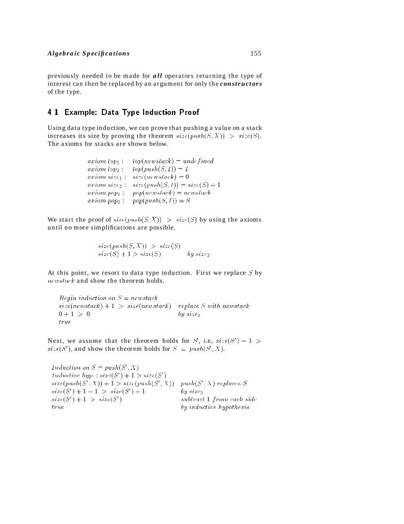
Algebraic Specifications 155
previously needed to be made for all operators returning the type ofinterest can then be replaced by an argument for only the constructorsof the type.
���� Example� Data Type Induction Proof
Using data type induction, we can prove that pushing a value on a stackincreases its size by proving the theorem size�push�S�X�� � size�S�.The axioms for stacks are shown below.
axiom top1 : top�newstack� � undefinedaxiom top2 : top�push�S� I�� � Iaxiom size1 : size�newstack� � 0axiom size2 : size�push�S� I�� � size�S� � 1axiom pop1 : pop�newstack� � newstackaxiom pop2 : pop�push�S� I�� � S
We start the proof of size�push�S�X�� � size�S� by using the axiomsuntil no more simplifications are possible.
size�push�S�X�� � size�S�size�S� � 1 � size�S� by size2
At this point, we resort to data type induction. First we replace S bynewstack and show the theorem holds.
Begin induction on S � newstacksize�newstack� � 1 � size�newstack� replace S with newstack0 � 1 � 0 by size1true
Next, we assume that the theorem holds for S�, i.e, size�S �� � 1 �size�S��� and show the theorem holds for S � push�S�� X�.
Induction on S � push�S�� X�Inductive hyp� : size�S�� � 1 � size�S��size�push�S� � X�� � 1 � size�push�S� � X�� push�S�� X� replaces Ssize�S�� � 1 � 1 � size�S�� � 1 by size2size�S�� � 1 � size�S�� subtract 1 from each sidetrue by inductive hypothesis
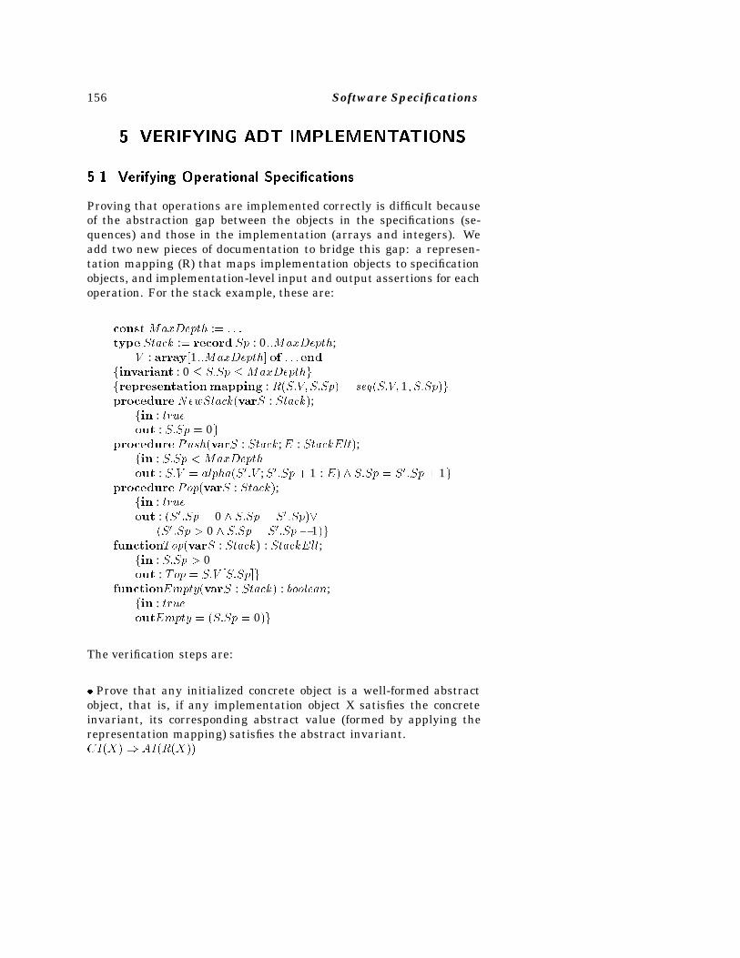
156 Software Specifications
�� VERIFYING ADT IMPLEMENTATIONS
���� Verifying Operational Speci�cations
Proving that operations are implemented correctly is difficult becauseof the abstraction gap between the objects in the specifications (se-quences) and those in the implementation (arrays and integers). Weadd two new pieces of documentation to bridge this gap: a represen-tation mapping (R) that maps implementation objects to specificationobjects, and implementation-level input and output assertions for eachoperation. For the stack example, these are:
constMaxDepth :� � � �type Stack :� record Sp : 0��MaxDepth;
V : array�1��MaxDepth� of � � �endfinvariant : 0 � S�Sp �MaxDepthgfrepresentationmapping : R�S�V� S�Sp� � seq�S�V� 1� S�Sp�gprocedure NewStack�varS : Stack�;
fin : trueout : S�Sp � 0g
procedure Push�varS : Stack;E : StackElt�;fin : S�Sp � MaxDepthout : S�V � alpha�S��V ;S��Sp � 1 : E� S�Sp � S��Sp� 1g
procedure Pop�varS : Stack�;fin : trueout : �S��Sp � 0 S�Sp � S��Sp��
�S��Sp � 0 S�Sp � S��Sp � 1�gfunctionTop�varS : Stack� : StackElt;
fin : S�Sp � 0out : Top � S�V �S�Sp�g
functionEmpty�varS : Stack� : boolean;fin : trueoutEmpty � �S�Sp � 0�g
The verification steps are:
� Prove that any initialized concrete object is a well-formed abstractobject, that is, if any implementation object X satisfies the concreteinvariant, its corresponding abstract value (formed by applying therepresentation mapping) satisfies the abstract invariant.CI�X� AI�R�X��
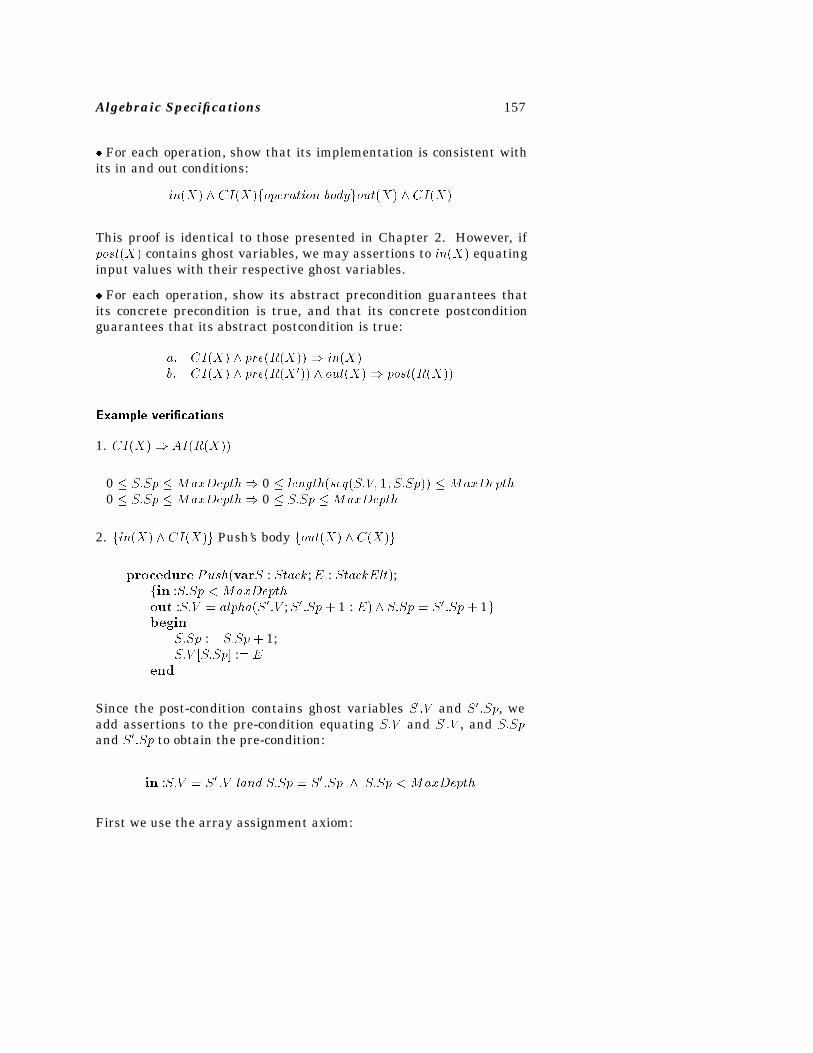
Algebraic Specifications 157
� For each operation, show that its implementation is consistent withits in and out conditions:
in�X� CI�X�foperation bodygout�X� CI�X�
This proof is identical to those presented in Chapter 2. However, ifpost�X� contains ghost variables, we may assertions to in�X� equatinginput values with their respective ghost variables.
� For each operation, show its abstract precondition guarantees thatits concrete precondition is true, and that its concrete postconditionguarantees that its abstract postcondition is true:
a� CI�X� pre�R�X�� in�X�b� CI�X� pre�R�X��� out�X� post�R�X��
Example veri�cations
1. CI�X� AI�R�X��
0 � S�Sp �MaxDepth 0 � length�seq�S�V� 1� S�Sp�� �MaxDepth0 � S�Sp �MaxDepth 0 � S�Sp �MaxDepth
2. fin�X� CI�X�g Push’s body fout�X� C�X�g
procedure Push�varS : Stack;E : StackElt�;fin :S�Sp � MaxDepthout :S�V � alpha�S��V ;S��Sp � 1 : E� S�Sp � S��Sp � 1gbegin
S�Sp :� S�Sp � 1;S�V �S�Sp� :� E
end
Since the post-condition contains ghost variables S��V and S��Sp, weadd assertions to the pre-condition equating S�V and S��V , and S�Spand S��Sp to obtain the pre-condition:
in :S�V � S��V land S�Sp � S��Sp S�Sp � MaxDepth
First we use the array assignment axiom:
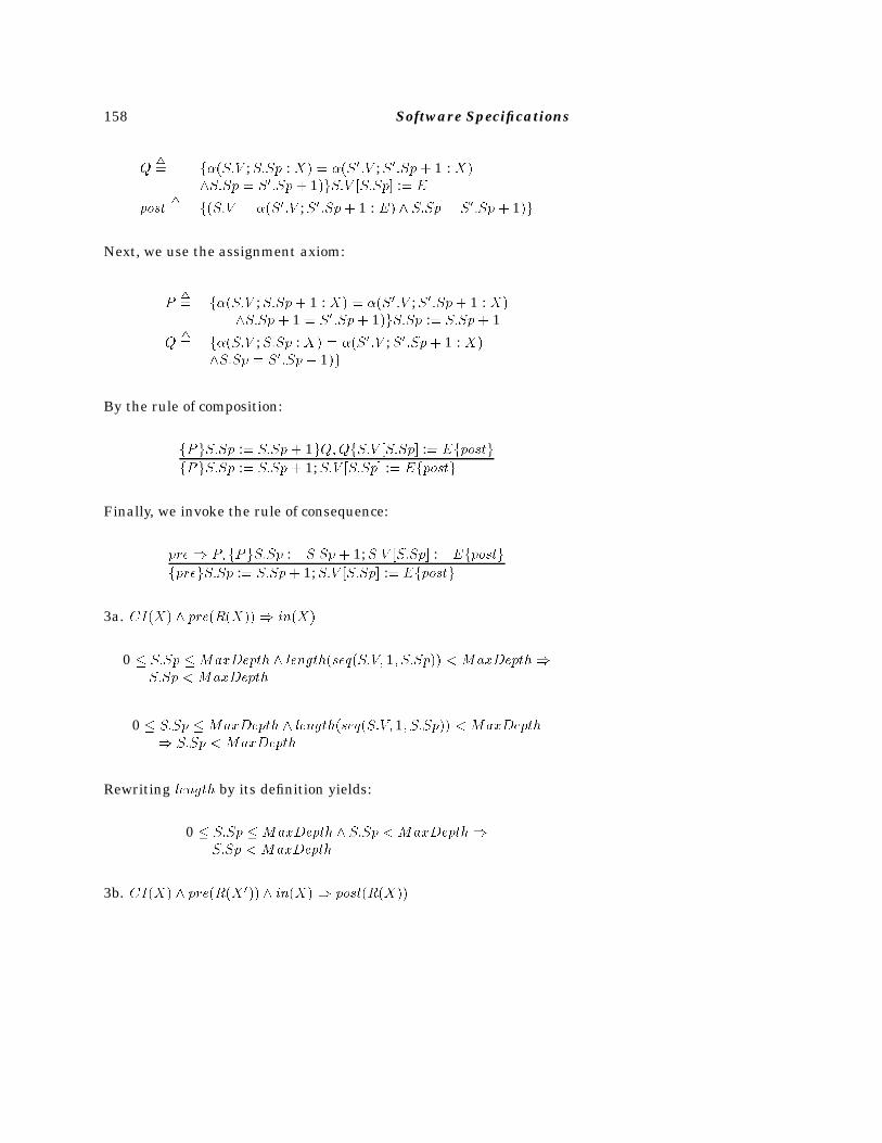
158 Software Specifications
Q�� f��S�V ;S�Sp : X� � ��S��V ;S��Sp � 1 : X�
S�Sp � S��Sp � 1�gS�V �S�Sp� :� E
post�� f�S�V � ��S��V ;S��Sp� 1 : E� S�Sp � S��Sp � 1�g
Next, we use the assignment axiom:
P�� f��S�V ;S�Sp� 1 : X� � ��S��V ;S��Sp� 1 : X�
S�Sp � 1 � S��Sp� 1�gS�Sp :� S�Sp � 1
Q�� f��S�V ;S�Sp : X� � ��S��V ;S��Sp� 1 : X�
S�Sp � S��Sp� 1�g
By the rule of composition:
fPgS�Sp :� S�Sp � 1gQ�QfS�V �S�Sp� :� Efpostg
fPgS�Sp :� S�Sp � 1;S�V �S�Sp� :� Efpostg
Finally, we invoke the rule of consequence:
pre P� fPgS�Sp :� S�Sp � 1;S�V �S�Sp� :� Efpostg
fpregS�Sp :� S�Sp � 1;S�V �S�Sp� :� Efpostg
3a. CI�X� pre�R�X�� in�X�
0 � S�Sp �MaxDepth length�seq�S�V� 1� S�Sp�� � MaxDepthS�Sp � MaxDepth
0 � S�Sp �MaxDepth length�seq�S�V� 1� S�Sp�� � MaxDepth S�Sp � MaxDepth
Rewriting length by its definition yields:
0 � S�Sp �MaxDepth S�Sp � MaxDepthS�Sp � MaxDepth
3b. CI�X� pre�R�X ��� in�X� post�R�X��
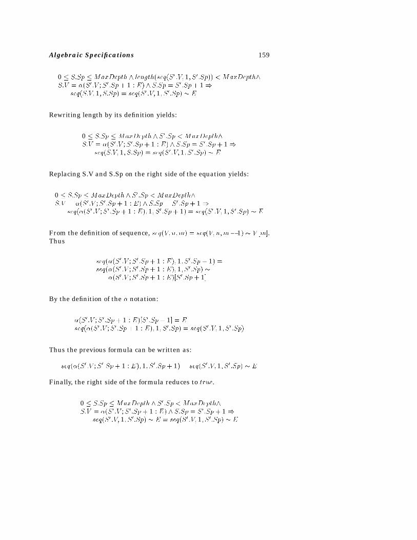
Algebraic Specifications 159
0 � S�Sp �MaxDepth length�seq�S� �V� 1� S��Sp�� � MaxDepthS�V � ��S��V ;S��Sp� 1 : E� S�Sp � S��Sp� 1
seq�S�V� 1� S�Sp� � seq�S��V� 1� S��Sp� � E
Rewriting length by its definition yields:
0 � S�Sp �MaxDepth S��Sp � MaxDepthS�V � ��S��V ;S��Sp � 1 : E� S�Sp � S��Sp� 1
seq�S�V� 1� S�Sp� � seq�S��V� 1� S��Sp� � E
Replacing S.V and S.Sp on the right side of the equation yields:
0 � S�Sp � MaxDepth S��Sp � MaxDepthS�V � ��S��V ;S��Sp � 1 : E� S�Sp � S��Sp� 1
seq���S��V ;S��Sp � 1 : E�� 1� S��Sp� 1� � seq�S� �V� 1� S��Sp� � E
From the definition of sequence, seq�V� n�m� � seq�V� n�m� 1� � V �m�.Thus
seq���S��V ;S��Sp� 1 : E�� 1� S��Sp � 1� �seq���S��V ;S��Sp� 1 : E�� 1� S��Sp� �
��S��V ;S��Sp� 1 : E��S��Sp� 1�
By the definition of the � notation:
��S��V ;S��Sp� 1 : E��S��Sp� 1� � Eseq���S��V ;S��Sp� 1 : E�� 1� S��Sp� � seq�S��V� 1� S��Sp�
Thus the previous formula can be written as:
seq���S��V ;S��Sp� 1 : E�� 1� S��Sp � 1� � seq�S��V� 1� S��Sp� � E
Finally, the right side of the formula reduces to true.
0 � S�Sp �MaxDepth S��Sp � MaxDepthS�V � ��S��V ;S��Sp� 1 : E� S�Sp � S��Sp � 1
seq�S��V� 1� S��Sp� � E � seq�S��V� 1� S��Sp� � E
160 Software Specifications
���� Verifying Algebraic Speci�cations
In operationally specified ADTs, the actions of operators were describedin terms of a distinct, concrete type; hence, their implementation is eas-ily discussed in terms of only that type. In contrast, the operators of analgebraically specified ADT are described by how they interrelate withthe other operators. There is no second (let alone concrete) type usedin this case. Therefore, to give an implementation of an algebraicallyspecified ADT, it is essential that we first describe the properties of asecond data type that will be used to implement the first. In keepingwith the spirit of this abstraction activity, we usually give an algebraicspecification for this second type as well.
We often refer to the type we are trying to implement as a “higher level”data type, and to the type used in the implementation as a “lower level”data type. However, these phrases are vague, and they only resultfrom the way we naturally think about the implementation process. Infact, the lower level type might itself be an elaborate ADT with richsemantics. It, in turn, might be implemented in terms of yet a lower-level type, and so on. A hierarchy of data types can often result inthis manner. The goal of course is for one of these lower level types toultimately be directly representable and implemented in hardware (forinstance, we will shortly show how to implement the STACKs specifiedearlier in terms of an algebraically specified array, and we would expectthat this array could be directly implemented in our host language onmost computers).
However, there is one glaring problem associated with this type hi-erarchy, and that is how to check whether a lower-level data type isfaithfully implemented on a real machine. In the example we areabout to give (STACKs in terms of arrays), our specification of arrayassumes that we have an unbounded array, and further, that uninitial-ized entries in the array can be detected. These properties are rarelytrue of machine implementations. Hence, our techniques are only asreliable as is our implementation of the base types. Nonetheless, if wedo develop a specification which can be reliably implemented on a ma-chine, then all the benefits of a verified implementation can be enjoyed.One of the most important of these benefits is that the machine-specificproperties that must be captured are very localized, that is, develop-ers will be free to use instances of our STACK data type, and it willbe transparent whether they are implemented using arrays (on somehardware) or actual stacks (on a stack machine).
Algebraic Specifications 161
Once we have the specification for both the higher- and lower-leveltypes, we can describe how the one is to be implemented in terms ofthe other. This is done through an implementation program, which,just as with the original specification of the individual ADTs, looks likea list of axioms. However, whereas before the axioms showed how theoperators from any one type lnterrelated, the implementation programshows how the higher-level type behaves in terms of the lower-leveltype.
In order to complete this implementation program, there is one ad-ditional, and quite essential, function which must be provided: therepresentation function. Remember that the operators from each in-dividual type are functions that map into different ranges. It wouldbe absurd to make an implementation program that then equates therange of one ADT’s operator with the range of a different ADT’s oper-ator. The program only makes sense when there is a representationfunction which shows how to map an instance of the lower-level typeinto an instance of the higher-level type. Then, more precisely, we canshow how the operators of the higher-level type behave in terms of therange of the representation function applied to operators of the lowerlevel type.
Another subtle requirement that is placed on us is to come up withan equivalence interpretation. The implementation program is a list ofequations, as described above. But remember that, in general, ques-tions of equality are very difficult to resolve. If we are to have any hopeof being able to verify properties of this program, then we must have areliable way to answer questions of equality in terms of the lower-leveltype. The emphasis is for an important distinction: An implementationand its associated equivalence interpretation do not resolve the prob-lem of checking equality within just the higher level type system. Theywill only allow us to check whether similar operations on instances ofthe lower-level type will produce (through the representation function)identical sentences in the language of the higher-level type.
We are now ready to summarize what it means to verify an implementa-tion of some ADT. The most obvious requirement is that the axioms forour type of interest are preserved through the implementation. Sincethe only way we mathematically characterize our ADT is through howthey interrelate with one another, the only place we can turn to checkthe reasonableness of an implementation is exactly this body of rules.These must be checked. A less obvious proof obligation is to verify thatour equality interpretation is in fact an equivalence relation. Finally,
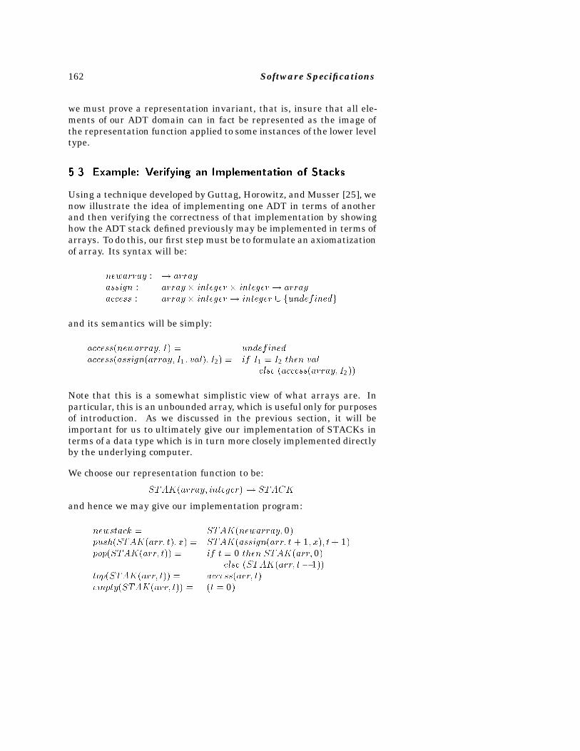
162 Software Specifications
we must prove a representation invariant, that is, insure that all ele-ments of our ADT domain can in fact be represented as the image ofthe representation function applied to some instances of the lower leveltype.
���� Example� Verifying an Implementation of Stacks
Using a technique developed by Guttag, Horowitz, and Musser [25], wenow illustrate the idea of implementing one ADT in terms of anotherand then verifying the correctness of that implementation by showinghow the ADT stack defined previously may be implemented in terms ofarrays. To do this, our first step must be to formulate an axiomatizationof array. Its syntax will be:
newarray : � arrayassign : array � integer � integer � arrayaccess : array � integer � integer � fundefinedg
and its semantics will be simply:
access�newarray� I� � undefinedaccess�assign�array� I1 � val�� I2� � if I1 � I2 then val
else �access�array� I2��
Note that this is a somewhat simplistic view of what arrays are. Inparticular, this is an unbounded array, which is useful only for purposesof introduction. As we discussed in the previous section, it will beimportant for us to ultimately give our implementation of STACKs interms of a data type which is in turn more closely implemented directlyby the underlying computer.
We choose our representation function to be:
STAK�array� integer� � STACK
and hence we may give our implementation program:
newstack � STAK�newarray� 0�push�STAK�arr� t�� x� � STAK�assign�arr� t � 1� x�� t� 1�pop�STAK�arr� t�� � if t � 0 then STAK�arr� 0�
else �STAK�arr� t� 1��top�STAK�arr� t�� � access�arr� t�empty�STAK�arr� t�� � �t � 0�
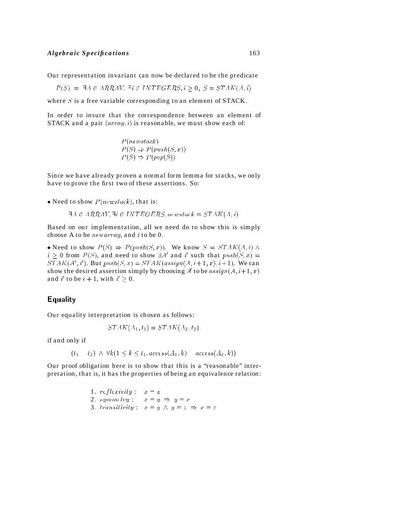
Algebraic Specifications 163
Our representation invariant can now be declared to be the predicate
P �S� � �A � ARRAY� �i � INTEGERS� i � 0� S � STAK�A� i�
where S is a free variable corresponding to an element of STACK.
In order to insure that the correspondence between an element ofSTACK and a pair �array� i� is reasonable, we must show each of:
P �newstack�P �S� P �push�S� x��P �S� P �pop�S��
Since we have already proven a normal form lemma for stacks, we onlyhave to prove the first two of these assertions. So:
� Need to show P �newstack�, that is:
�A � ARRAY� �i � INTEGERS� newstack � STAK�A� i�
Based on our implementation, all we need do to show this is simplychoose A to be newarray, and i to be 0.
� Need to show P �S� P �push�S� x��. We know S � STAK�A� i� i � 0 from P �S�, and need to show �A� and i� such that push�S� x� �STAK�A�� i��. But push�S� x� � STAK�assign�A� i�1� x�� i�1�. We canshow the desired assertion simply by choosing A� to be assign�A� i�1� x�and i� to be i � 1, with i� � 0.
Equality
Our equality interpretation is chosen as follows:
STAK�A1 � t1� � STAK�A2 � t2�
if and only if
�t1 � t2� �k�1 � k � t1� access�A1� k� � access�A2 � k��
Our proof obligation here is to show that this is a “reasonable” inter-pretation, that is, it has the properties of being an equivalence relation:
1� reflexivity : x � x2� symmetry : x � y y � x3� transitivity : x � y y � z x � z
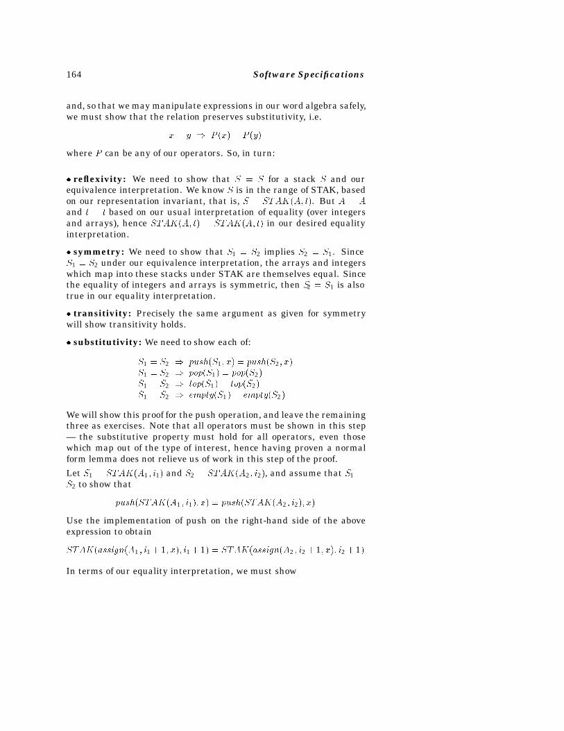
164 Software Specifications
and, so that we may manipulate expressions in our word algebra safely,we must show that the relation preserves substitutivity, i.e.
x � y P �x� � P �y�
where P can be any of our operators. So, in turn:
� reflexivity: We need to show that S � S for a stack S and ourequivalence interpretation. We know S is in the range of STAK, basedon our representation invariant, that is, S � STAK�A� t�. But A � Aand t � t based on our usual interpretation of equality (over integersand arrays), hence STAK�A� t� � STAK�A� t� in our desired equalityinterpretation.
� symmetry: We need to show that S1 � S2 implies S2 � S1. SinceS1 � S2 under our equivalence interpretation, the arrays and integerswhich map into these stacks under STAK are themselves equal. Sincethe equality of integers and arrays is symmetric, then S2 � S1 is alsotrue in our equality interpretation.
� transitivity: Precisely the same argument as given for symmetrywill show transitivity holds.
� substitutivity: We need to show each of:
S1 � S2 push�S1� x� � push�S2� x�S1 � S2 pop�S1� � pop�S2�S1 � S2 top�S1� � top�S2�S1 � S2 empty�S1� � empty�S2�
We will show this proof for the push operation, and leave the remainingthree as exercises. Note that all operators must be shown in this step— the substitutive property must hold for all operators, even thosewhich map out of the type of interest, hence having proven a normalform lemma does not relieve us of work in this step of the proof.
Let S1 � STAK�A1� i1� and S2 � STAK�A2 � i2�, and assume that S1 �S2 to show that
push�STAK�A1 � i1�� x� � push�STAK�A2 � i2�� x�
Use the implementation of push on the right-hand side of the aboveexpression to obtain
STAK�assign�A1 � i1 � 1� x�� i1 � 1� � STAK�assign�A2 � i2 � 1� x�� i2 � 1�
In terms of our equality interpretation, we must show
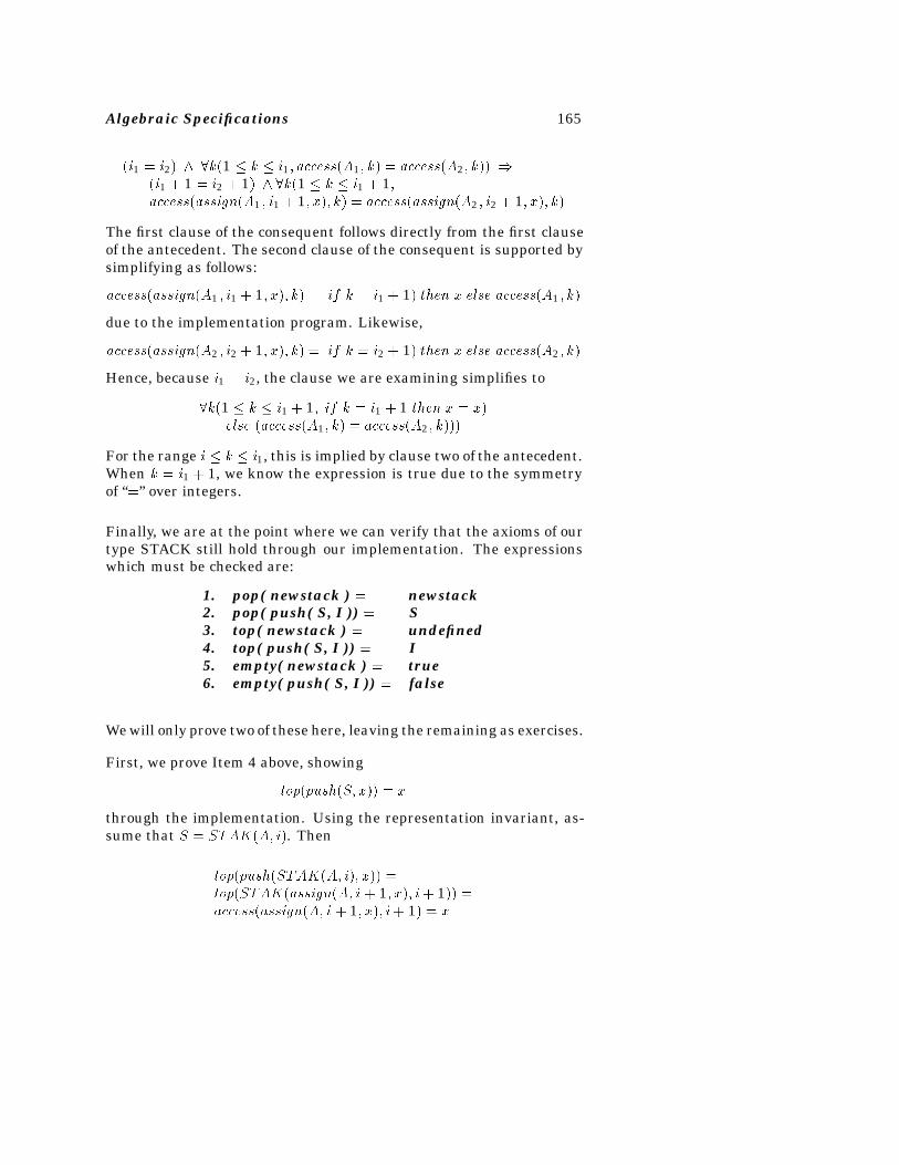
Algebraic Specifications 165
�i1 � i2� �k�1 � k � i1� access�A1� k� � access�A2� k�� �i1 � 1 � i2 � 1� �k�1 � k � i1 � 1�access�assign�A1 � i1 � 1� x�� k� � access�assign�A2 � i2 � 1� x�� k�
The first clause of the consequent follows directly from the first clauseof the antecedent. The second clause of the consequent is supported bysimplifying as follows:
access�assign�A1 � i1 � 1� x�� k� � if k � i1 � 1� then x else access�A1 � k�
due to the implementation program. Likewise,
access�assign�A2 � i2 � 1� x�� k� � if k � i2 � 1� then x else access�A2 � k�
Hence, because i1 � i2, the clause we are examining simplifies to
�k�1 � k � i1 � 1� if k � i1 � 1 then x � x�else �access�A1� k� � access�A2 � k���
For the range i � k � i1, this is implied by clause two of the antecedent.When k � i1 � 1, we know the expression is true due to the symmetryof “�” over integers.
Finally, we are at the point where we can verify that the axioms of ourtype STACK still hold through our implementation. The expressionswhich must be checked are:
1. pop( newstack ) � newstack2. pop( push( S, I )) � S3. top( newstack ) � undefined4. top( push( S, I )) � I5. empty( newstack ) � true6. empty( push( S, I )) � false
We will only prove two of these here, leaving the remaining as exercises.
First, we prove Item 4 above, showing
top�push�S� x�� � x
through the implementation. Using the representation invariant, as-sume that S � STAK�A� i�. Then
top�push�STAK�A� i�� x�� �top�STAK�assign�A� i � 1� x�� i� 1�� �access�assign�A� i � 1� x�� i� 1� � x
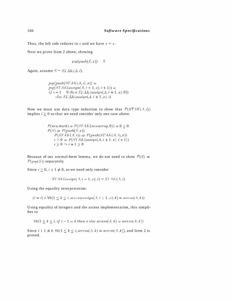
166 Software Specifications
Thus, the left side reduces to x and we have x � x.
Next we prove Item 2 above, showing
pop�push�S� x�� � S
Again, assume S � STAK�A� i�.
pop�push�STAK�A� i�� x�� �pop�STAK�assign�A� i � 1� x�� i� 1�� �if i � 1 � 0 then STAK�assign�A� i � 1� x�� 0��
else STAK�assign�A� i � 1� x�� i�
Now we must use data type induction to show that P �STAK�A� i��implies i � 0 so that we need consider only one case above.
P �newstack� � P �STAK�newarray� 0�� � 0 � 0�P �S� P �push�S� x��
P �STAK�A� i�� P �push�STAK�A� i�� x��i � 0 P �STAK�assign�A� i � 1� x�� i� 1��i � 0 i � 1 � 0
Because of our normal-form lemma, we do not need to show P �S� P �pop�S�� separately.
Since i � 0, i � 1 �� 0, so we need only consider
STAK�assign�A� i � 1� x�� i� � STAK�A� i�
Using the equality interpretation:
�i � i� �k�1 � k � i� access�assign�A� i � 1� x�� k� � access�A� k��
Using equality of integers and the access implementation, this simpli-fies to
�k�1 � k � i� if i� 1 � k then x else access�A� k� � access�A� k��
Since i� 1 �� k� �k�1 � k � i� access�A� k� � access�A� k��, and Item 2 isproved.
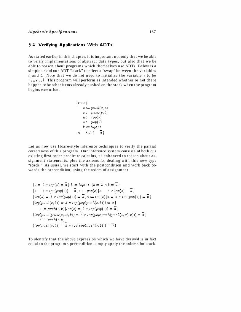
Algebraic Specifications 167
���� Verifying Applications With ADTs
As stated earlier in this chapter, it is important not only that we be ableto verify implementations of abstract data types, but also that we beable to reason about programs which themselves use ADTs. Below is asimple use of our ADT “stack” to effect a “swap” between the variablesa and b. Note that we do not need to initialize the variable s to benewstack. This program will perform as intended whether or not therehappen to be other items already pushed on the stack when the programbegins execution.
ftruegs :� push�s� a�s :� push�s� b�a :� top�s�s :� pop�s�b :� top�s�
fa ��
b b ��ag
Let us now use Hoare-style inference techniques to verify the partialcorrectness of this program. Our inference system consists of both ourexisting first order predicate calculus, as enhanced to reason about as-signment statements, plus the axioms for dealing with this new type“stack.” As usual, we start with the postcondition and work back to-wards the precondition, using the axiom of assignment:
fa ��
b top�s� ��ag b :� top�s� fa �
�
b b ��ag
fa ��
b top�pop�s�� ��ags :� pop�s�fa �
�
b top�s� ��ag
ftop�s� ��
b top�pop�s�� ��aga :� top�s�fa �
�
b top�pop�s�� ��ag
ftop�push�s� b�� ��
b top�pop�push�s� b��� ��ag
s :� push�s� b�ftop�s� ��
b top�pop�s�� ��ag
ftop�push�push�s� a�� b�� ��
b top�pop�push�push�s� a�� b��� ��ag
s :� push�s� a�
ftop�push�s� b�� ��
b top�pop�push�s� b��� ��ag
To identify that the above expression which we have derived is in factequal to the program’s precondition, simply apply the axioms for stack.
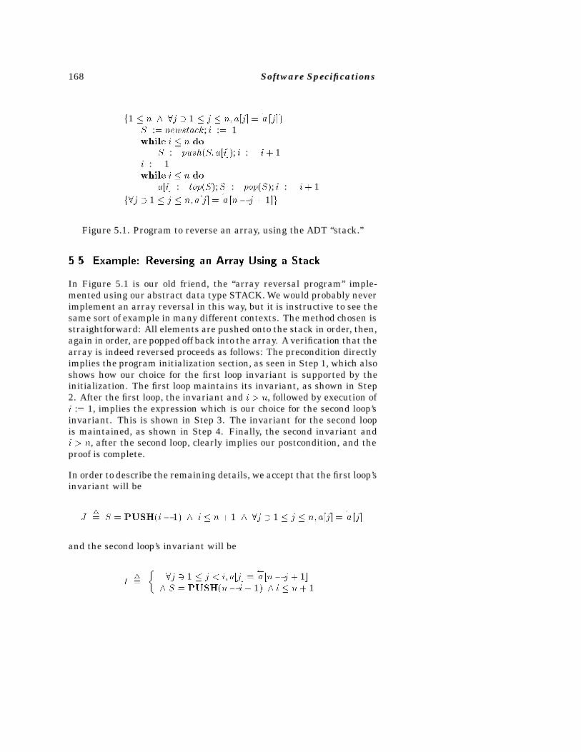
168 Software Specifications
f1 � n �j � 1 � j � n� a�j� ��a �j�g
S :� newstack; i :� 1while i � n do
S :� push�S� a�i��; i :� i � 1i :� 1while i � n do
a�i� :� top�S�;S :� pop�S�; i :� i � 1f�j � 1 � j � n� a�j� �
�a �n� j � 1�g
Figure 5.1. Program to reverse an array, using the ADT “stack.”
���� Example� Reversing an Array Using a Stack
In Figure 5.1 is our old friend, the “array reversal program” imple-mented using our abstract data type STACK. We would probably neverimplement an array reversal in this way, but it is instructive to see thesame sort of example in many different contexts. The method chosen isstraightforward: All elements are pushed onto the stack in order, then,again in order, are popped off back into the array. A verification that thearray is indeed reversed proceeds as follows: The precondition directlyimplies the program initialization section, as seen in Step 1, which alsoshows how our choice for the first loop invariant is supported by theinitialization. The first loop maintains its invariant, as shown in Step2. After the first loop, the invariant and i � n, followed by execution ofi :� 1, implies the expression which is our choice for the second loop’sinvariant. This is shown in Step 3. The invariant for the second loopis maintained, as shown in Step 4. Finally, the second invariant andi � n, after the second loop, clearly implies our postcondition, and theproof is complete.
In order to describe the remaining details, we accept that the first loop’sinvariant will be
J�� S � PUSH�i � 1� i � n � 1 �j � 1 � j � n� a�j� �
�a �j�
and the second loop’s invariant will be
I��
��j � 1 � j � i� a�j� �
�a �n� j � 1�
S � PUSH�n� i� 1� i � n� 1
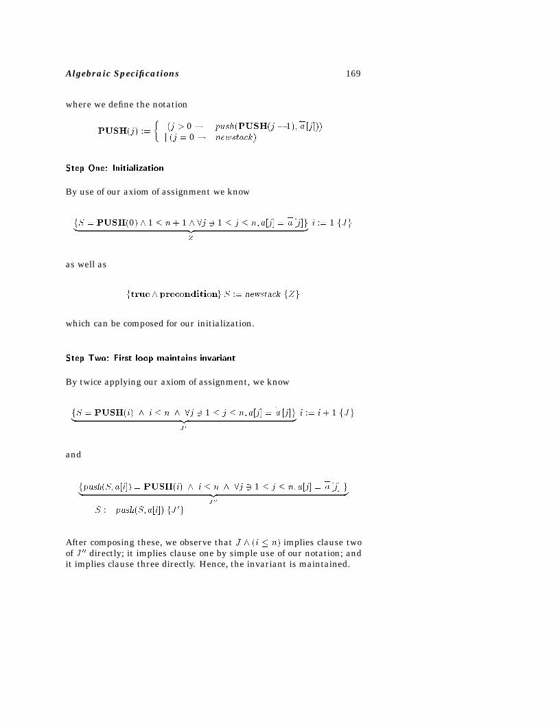
Algebraic Specifications 169
where we define the notation
PUSH�j� :��
�j � 0 � push�PUSH�j � 1���a �j���
j �j � 0 � newstack�
Step One� Initialization
By use of our axiom of assignment we know
fS � PUSH�0� 1 � n� 1 �j � 1 � j � n� a�j� ��a �j�g� �z �
Z
i :� 1 fJg
as well as
ftruepreconditiong S :� newstack fZg
which can be composed for our initialization.
Step Two� First loop maintains invariant
By twice applying our axiom of assignment, we know
fS � PUSH�i� i � n �j � 1 � j � n� a�j� ��a �j�g� �z �
J �
i :� i� 1 fJg
and
fpush�S� a�i�� � PUSH�i� i � n �j � 1 � j � n� a�j� ��a �j� g� �z �
J ��
S :� push�S� a�i�� fJ �g
After composing these, we observe that J �i � n� implies clause twoof J �� directly; it implies clause one by simple use of our notation; andit implies clause three directly. Hence, the invariant is maintained.
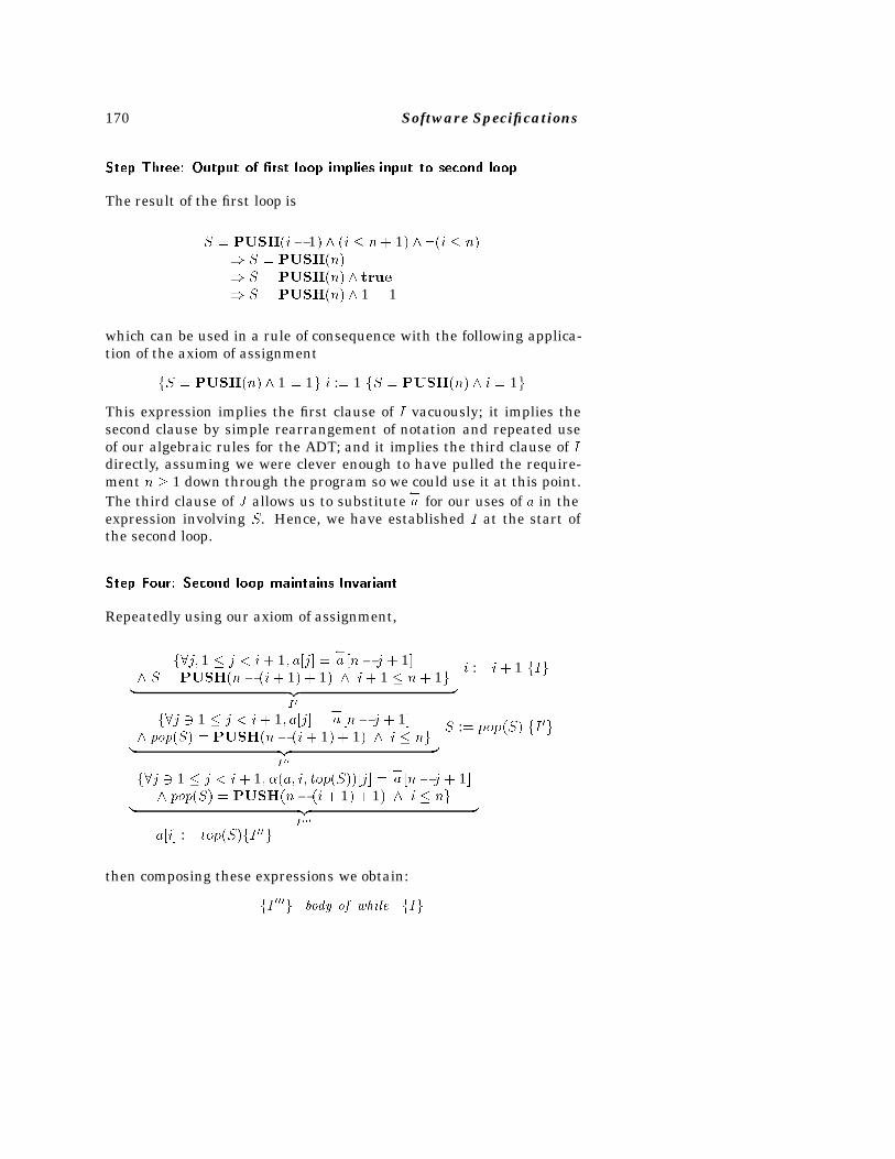
170 Software Specifications
Step Three� Output of �rst loop implies input to second loop
The result of the first loop is
S � PUSH�i� 1� �i � n� 1� ��i � n� S � PUSH�n� S � PUSH�n� true S � PUSH�n� 1 � 1
which can be used in a rule of consequence with the following applica-tion of the axiom of assignment
fS � PUSH�n� 1 � 1g i :� 1 fS � PUSH�n� i � 1g
This expression implies the first clause of I vacuously; it implies thesecond clause by simple rearrangement of notation and repeated useof our algebraic rules for the ADT; and it implies the third clause of Idirectly, assuming we were clever enough to have pulled the require-ment n � 1 down through the program so we could use it at this point.The third clause of J allows us to substitute
�a for our uses of a in the
expression involving S. Hence, we have established I at the start ofthe second loop.
Step Four� Second loop maintains Invariant
Repeatedly using our axiom of assignment,
f�j� 1 � j � i � 1� a�j� ��a �n� j � 1�
S � PUSH�n � �i � 1� � 1� i� 1 � n� 1g� �z �I�
i :� i � 1 fIg
f�j � 1 � j � i� 1� a�j� ��a �n� j � 1�
pop�S� � PUSH�n� �i � 1� � 1� i � ng� �z �I��
S :� pop�S� fI �g
f�j � 1 � j � i � 1� ��a� i� top�S���j� ��a �n� j � 1�
pop�S� � PUSH�n� �i � 1� � 1� i � ng� �z �I���
a�i� :� top�S�fI ��g
then composing these expressions we obtain:
fI ���g body of while fIg
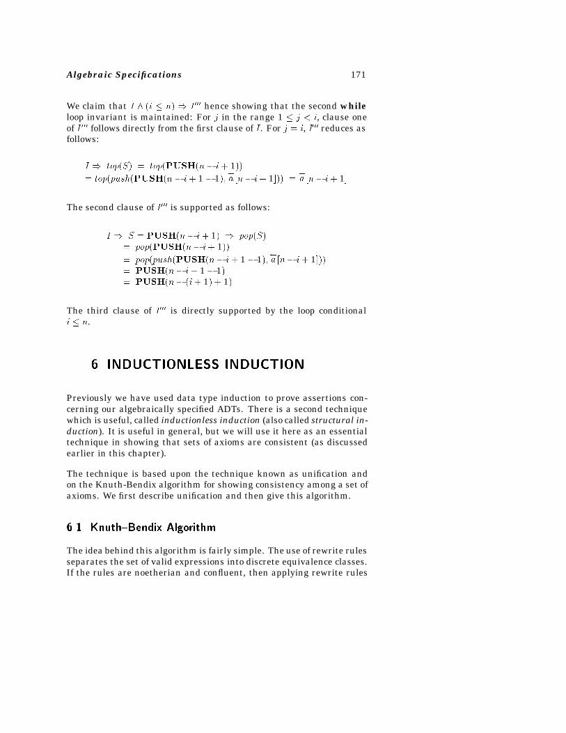
Algebraic Specifications 171
We claim that I �i � n� I��� hence showing that the second whileloop invariant is maintained: For j in the range 1 � j � i, clause oneof I ��� follows directly from the first clause of I. For j � i, I��� reduces asfollows:
I top�S� � top�PUSH�n� i � 1��� top�push�PUSH�n � i � 1 � 1��
�a �n� i � 1��� �
�a �n� i � 1�
The second clause of I��� is supported as follows:
I S � PUSH�n � i � 1� pop�S�� pop�PUSH�n� i� 1��� pop�push�PUSH�n� i� 1� 1��
�a �n� i� 1���
� PUSH�n� i� 1� 1�� PUSH�n� �i� 1� � 1�
The third clause of I��� is directly supported by the loop conditionali � n.
�� INDUCTIONLESS INDUCTION
Previously we have used data type induction to prove assertions con-cerning our algebraically specified ADTs. There is a second techniquewhich is useful, called inductionless induction (also called structural in-duction). It is useful in general, but we will use it here as an essentialtechnique in showing that sets of axioms are consistent (as discussedearlier in this chapter).
The technique is based upon the technique known as unification andon the Knuth-Bendix algorithm for showing consistency among a set ofaxioms. We first describe unification and then give this algorithm.
���� KnuthBendix Algorithm
The idea behind this algorithm is fairly simple. The use of rewrite rulesseparates the set of valid expressions into discrete equivalence classes.If the rules are noetherian and confluent, then applying rewrite rules
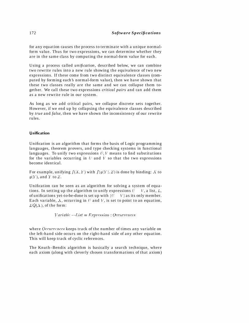
172 Software Specifications
for any equation causes the process to terminate with a unique normal-form value. Thus for two expressions, we can determine whether theyare in the same class by computing the normal-form value for each.
Using a process called unification, described below, we can combinetwo rewrite rules into a new rule showing the equivalence of two newexpressions. If these come from two distinct equivalence classes (com-puted by forming each’s normal-form value), then we have shown thatthese two classes really are the same and we can collapse them to-gether. We call these two expressions critical pairs and can add themas a new rewrite rule in our system.
As long as we add critical pairs, we collapse discrete sets together.However, if we end up by collapsing the equivalence classes describedby true and false, then we have shown the inconsistency of our rewriterules.
Uni�cation
Unification is an algorithm that forms the basis of Logic programminglanguages, theorem provers, and type checking systems in functionallanguages. To unify two expressions U� V means to find substitutionsfor the variables occurring in U and V so that the two expressionsbecome identical.
For example, unifying f�X�Y � with f�g�Y �� Z� is done by binding: X tog�Y �, and Y to Z.
Unification can be seen as an algorithm for solving a system of equa-tions. In setting up the algorithm to unify expressions U � V , a list, L,of unifications yet-to-be-done is set up with �U � V � as its only member.Each variable, X, occurring in U and V , is set to point to an equation,EQ�X�, of the form:
V ariable � List � Expression : Occurrences
where Occurrences keeps track of the number of times any variable onthe left-hand side occurs on the right-hand side of any other equation.This will keep track of cyclic references.
The Knuth–Bendix algorithm is basically a search technique, whereeach axiom (along with cleverly chosen transformations of that axiom)
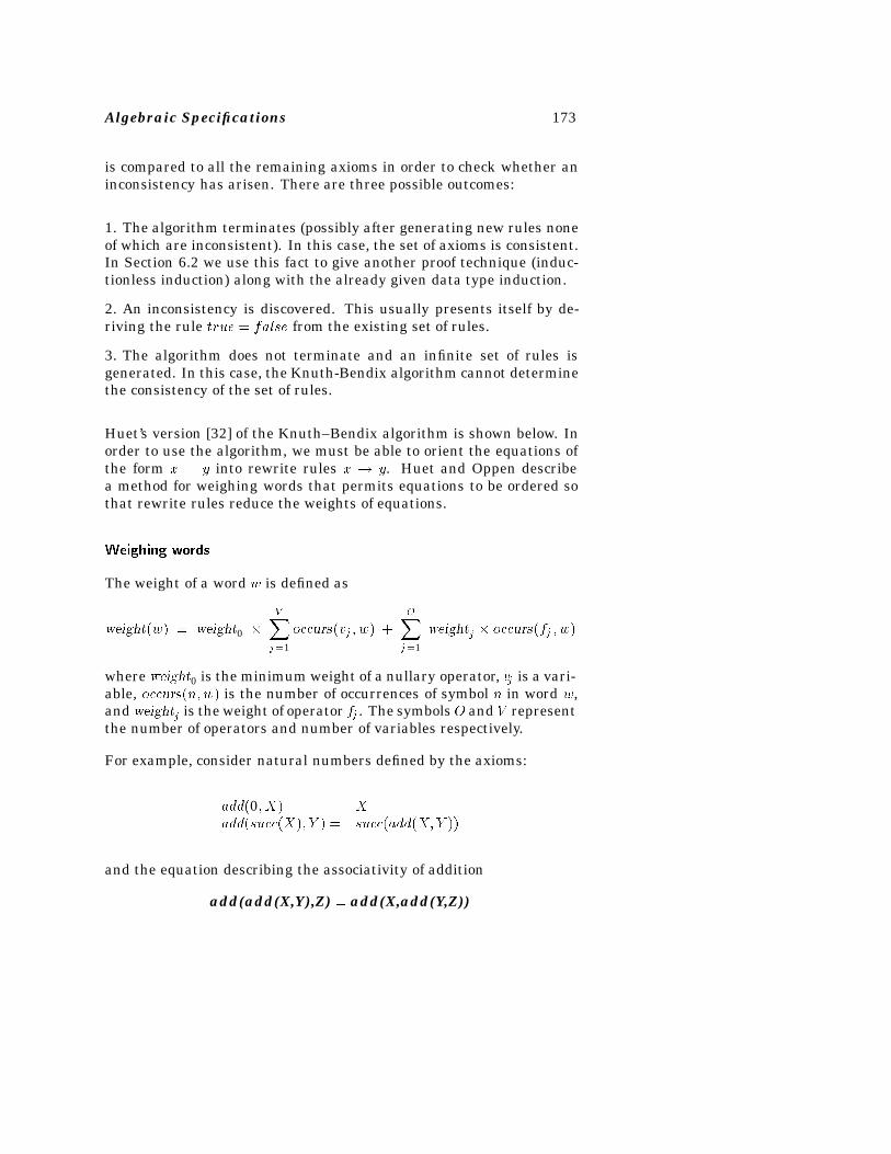
Algebraic Specifications 173
is compared to all the remaining axioms in order to check whether aninconsistency has arisen. There are three possible outcomes:
1. The algorithm terminates (possibly after generating new rules noneof which are inconsistent). In this case, the set of axioms is consistent.In Section 6.2 we use this fact to give another proof technique (induc-tionless induction) along with the already given data type induction.
2. An inconsistency is discovered. This usually presents itself by de-riving the rule true � false from the existing set of rules.
3. The algorithm does not terminate and an infinite set of rules isgenerated. In this case, the Knuth-Bendix algorithm cannot determinethe consistency of the set of rules.
Huet’s version [32] of the Knuth–Bendix algorithm is shown below. Inorder to use the algorithm, we must be able to orient the equations ofthe form x � y into rewrite rules x � y. Huet and Oppen describea method for weighing words that permits equations to be ordered sothat rewrite rules reduce the weights of equations.
Weighing words
The weight of a word w is defined as
weight�w� � weight0 �VXj�1
occurs�vj� w� �OXj�1
weightj � occurs�fj � w�
where weight0 is the minimum weight of a nullary operator, vj is a vari-able, occurs�n�w� is the number of occurrences of symbol n in word w,and weightj is the weight of operator fj . The symbolsO and V representthe number of operators and number of variables respectively.
For example, consider natural numbers defined by the axioms:
add�0� X� � Xadd�succ�X�� Y � � succ�add�X�Y ��
and the equation describing the associativity of addition
add(add(X,Y),Z) � add(X,add(Y,Z))
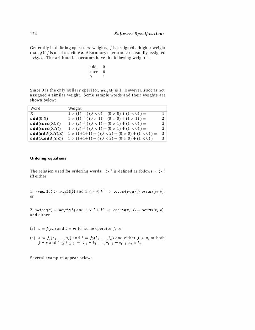
174 Software Specifications
Generally in defining operators’ weights, f is assigned a higher weightthan g if f is used to define g. Also unary operators are usually assignedweight0. The arithmetic operators have the following weights:
add 0succ 00 1
Since 0 is the only nullary operator, weight0 is 1. However, succ is notassigned a similar weight. Some sample words and their weights areshown below:
Word WeightX 1 � (1) � ( (0 � 0) � (0 � 0) � (1 � 0) ) � 1add(0,X) 1 � (1) � ( (0 � 1) � (0 � 0) � (1 � 1) ) � 2add(succ(X),Y) 1 � (2) � ( (0 � 1) � (0 � 1) � (1 � 0) ) � 2add(succ(X,Y)) 1 � (2) � ( (0 � 1) � (0 � 1) � (1 � 0) ) � 2add(add(X,Y),Z) 1 � (1�1�1) � ( (0 � 2) � (0 � 0) � (1 � 0) ) � 3add(X,add(Y,Z)) 1 � (1�1�1) � ( (0 � 2) � (0 � 0) � (1 � 0) ) � 3
Ordering equations
The relation used for ordering words a � b is defined as follows: a � biff either
1. weight�a� � weight�b� and 1 � i � V occurs�vi� a� � occurs�vi� b�;or
2. weight�a� � weight�b� and 1 � i � V occurs�vi� a� � occurs�vi� b�,and either
(a) a � f�vk� and b � vk for some operator f , or
(b) a � fj�a1� � � � � aj� and b � fk�b1� � � � � bk� and either j � k, or bothj � k and 1 � t � j a1 � b1� � � � � at�1 � bt�1� at � bt�
Several examples appear below:
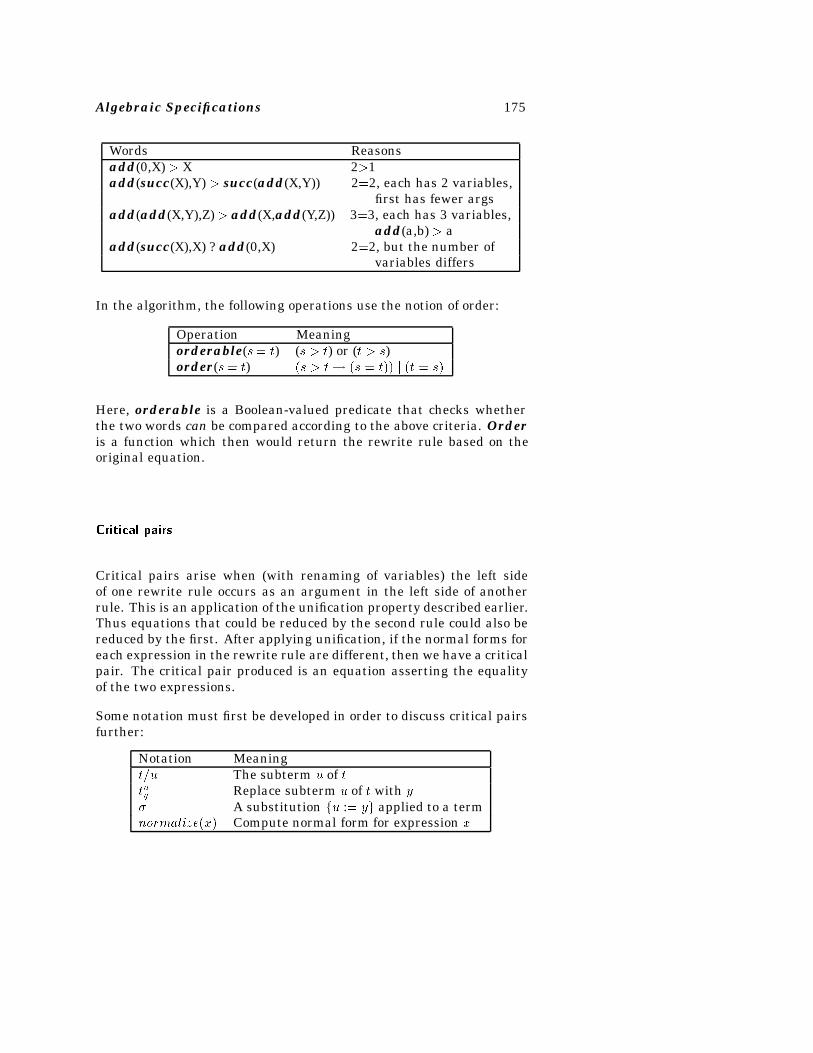
Algebraic Specifications 175
Words Reasonsadd(0,X) � X 2�1add(succ(X),Y) � succ(add(X,Y)) 2�2, each has 2 variables,
first has fewer argsadd(add(X,Y),Z)� add(X,add(Y,Z)) 3�3, each has 3 variables,
add(a,b) � aadd(succ(X),X) ? add(0,X) 2�2, but the number of
variables differs
In the algorithm, the following operations use the notion of order:
Operation Meaningorderable(s� t) (s � t) or (t � s)order(s � t) �s � t� �s � t�� j �t � s�
Here, orderable is a Boolean-valued predicate that checks whetherthe two words can be compared according to the above criteria. Orderis a function which then would return the rewrite rule based on theoriginal equation.
Critical pairs
Critical pairs arise when (with renaming of variables) the left sideof one rewrite rule occurs as an argument in the left side of anotherrule. This is an application of the unification property described earlier.Thus equations that could be reduced by the second rule could also bereduced by the first. After applying unification, if the normal forms foreach expression in the rewrite rule are different, then we have a criticalpair. The critical pair produced is an equation asserting the equalityof the two expressions.
Some notation must first be developed in order to discuss critical pairsfurther:
Notation Meaningtu The subterm u of ttuy Replace subterm u of t with y� A substitution fu :� yg applied to a termnormalize�x� Compute normal form for expression x
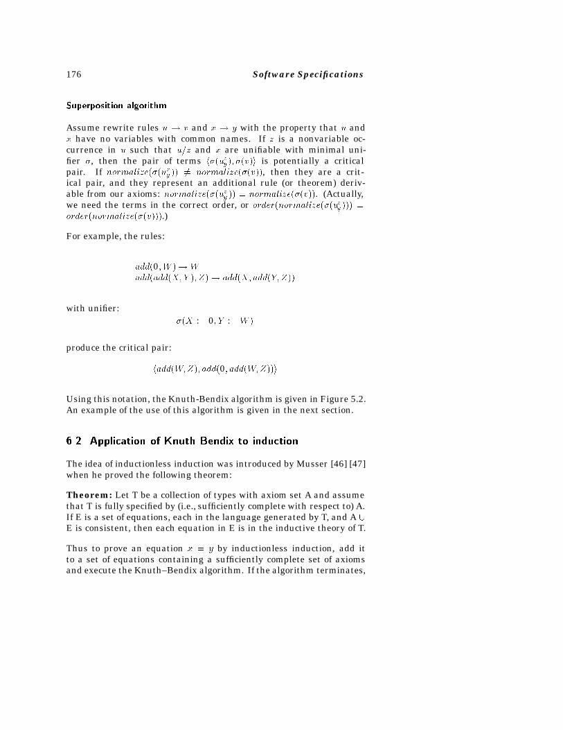
176 Software Specifications
Superposition algorithm
Assume rewrite rules u � v and x � y with the property that u andx have no variables with common names. If z is a nonvariable oc-currence in u such that uz and x are unifiable with minimal uni-fier �, then the pair of terms h��uzy�� ��v�i is potentially a criticalpair. If normalize���uzy�� �� normalize���v��, then they are a crit-ical pair, and they represent an additional rule (or theorem) deriv-able from our axioms: normalize���uzy �� � normalize���v��. (Actually,we need the terms in the correct order, or order�normalize���uzy��� �order�normalize���v���.)
For example, the rules:
add�0�W ��Wadd�add�X�Y �� Z�� add�X� add�Y� Z��
with unifier:��X :� 0� Y :� W �
produce the critical pair:
hadd�W�Z�� add�0� add�W�Z��i
Using this notation, the Knuth-Bendix algorithm is given in Figure 5.2.An example of the use of this algorithm is given in the next section.
���� Application of Knuth Bendix to induction
The idea of inductionless induction was introduced by Musser [46] [47]when he proved the following theorem:
Theorem: Let T be a collection of types with axiom set A and assumethat T is fully specified by (i.e., sufficiently complete with respect to) A.If E is a set of equations, each in the language generated by T, and A �E is consistent, then each equation in E is in the inductive theory of T.
Thus to prove an equation x � y by inductionless induction, add itto a set of equations containing a sufficiently complete set of axiomsand execute the Knuth–Bendix algorithm. If the algorithm terminates,
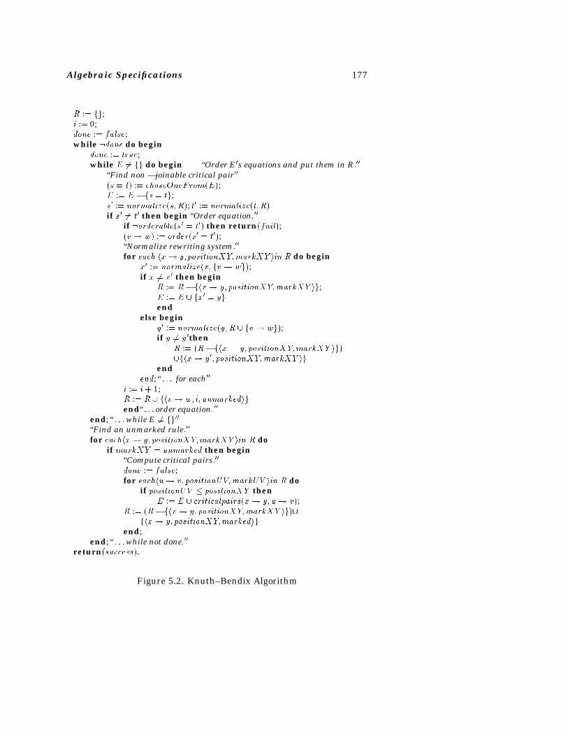
Algebraic Specifications 177
R :� fg;i :� 0;done :� false;while �done do begin
done :� true;while E �� fg do begin “Order E�s equations and put them in R���
“Find non� joinable critical pair��
�s � t� :� choseOneFrom�E�;E :� E � fs � tg;s� :� normalize�s�R�; t� :� normalize�t�R�if s� �� t� then begin “Order equation���
if �orderable�s� � t�� then return�fail�;�v� w� :� order�s� � t��;“Normalize rewriting system���
for each hx� y� positionXY�markXY iin R do beginx� :� normalize�x� fv � wg�;if x �� x� then begin
R :� R� fhx� y� positionXY�markXY ig;E :� E � fx� � ygend
else beginy� :� normalize�y�R � fv � wg�;if y �� y�then
R :� �R� fhx� y� positionXY�markXY ig��fhx� y�� positionXY�markXY ig
endend; “ � � � for each��
i :� i� 1;R :� R � fhv� w� i� unmarkedigend“ � � � order equation���
end; “ � � �while E �� fg��
“Find an unmarked rule���
for eachhx� y� positionXY�markXY iin R doif markXY � unmarked then begin
“Compute critical pairs���
done :� false;for eachhu� v� positionUV�markUV iin R do
if positionUV � positionXY thenE :� E � criticalpairs�x� y� u� v�;
R :� �R� fhx� y� positionXY�markXY ig��fhx� y� positionXY�markedig
end;end; “ � � �while not done���
return�success��
Figure 5.2. Knuth–Bendix Algorithm
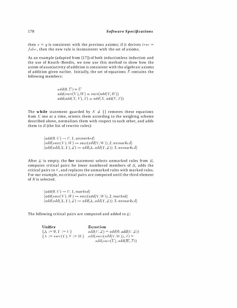
178 Software Specifications
then x � y is consistent with the previous axioms; if it derives true �false, then the new rule is inconsistent with the set of axioms.
As an example (adapted from [17]) of both inductionless induction andthe use of Knuth–Bendix, we now use this method to show how theaxiom of associativity of addition is consistent with the algebraic axiomsof addition given earlier. Initially, the set of equations E contains thefollowing members:
add�0� U � � Uadd�succ�V ��W � � succ�add�V�W ��add�add�X�Y �� Z� � add�X� add�Y� Z��
The while statement guarded by E �� fg removes these equationsfrom E one at a time, orients them according to the weighing schemedescribed above, normalizes them with respect to each other, and addsthem to R (the list of rewrite rules):
hadd�0� U �� U� 1� unmarkedihadd�succ�V ��W �� succ�add�V�W ��� 2� unmarkedihadd�add�X�Y �� Z� � add�X� add�Y� Z��� 3� unmarkedi
After E is empty, the for statement selects unmarked rules from R,computes critical pairs for lower numbered members of R, adds thecritical pairs toE, and replaces the unmarked rules with marked rules.For our example, no critical pairs are computed until the third elementof R is selected.
hadd�0� U �� U� 1�markedihadd�succ�V ��W �� succ�add�V�W ��� 2�markedihadd�add�X�Y �� Z� � add�X� add�Y� Z��� 3� unmarkedi
The following critical pairs are computed and added to E:
Uni�er Equation
fX :� 0� Y :� Ug add�U�Z� � add�0� add�U�Z��fX :� succ�V �� Y :� Wg add�succ�add�V�W ��� Z� �
add�succ�V �� add�W�Z��
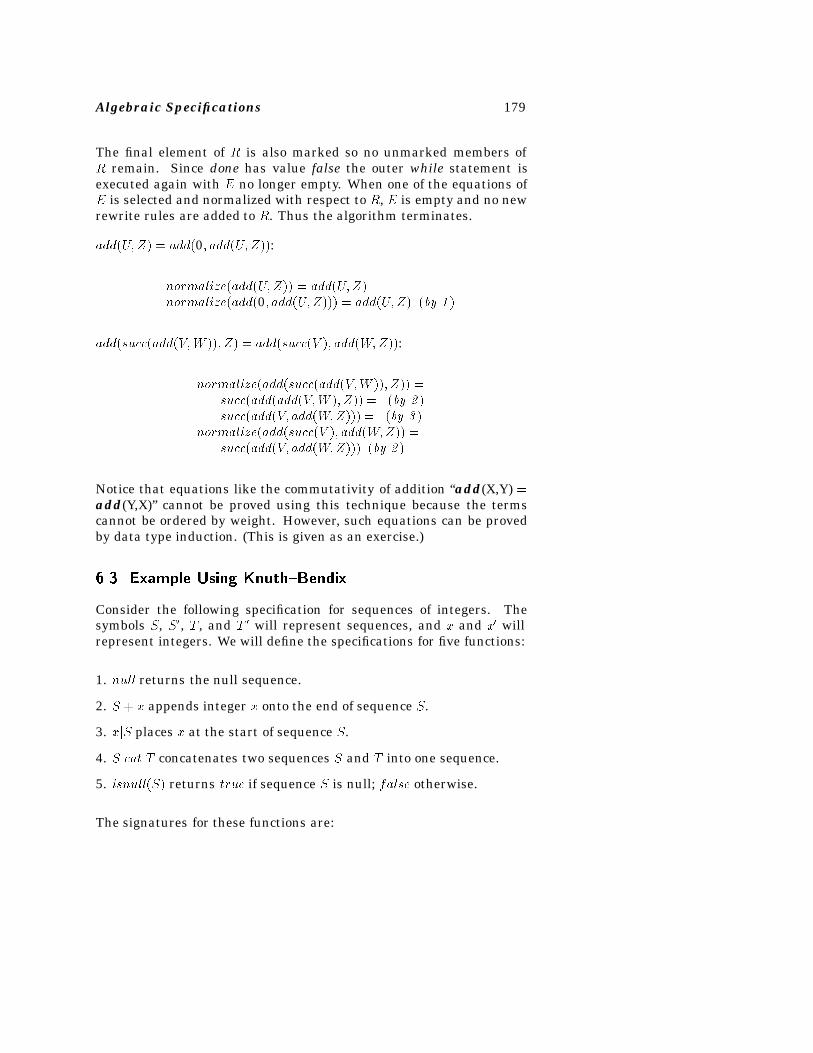
Algebraic Specifications 179
The final element of R is also marked so no unmarked members ofR remain. Since done has value false the outer while statement isexecuted again with E no longer empty. When one of the equations ofE is selected and normalized with respect to R, E is empty and no newrewrite rules are added to R. Thus the algorithm terminates.
add�U�Z� � add�0� add�U�Z��:
normalize�add�U�Z�� � add�U�Z�normalize�add�0� add�U�Z��� � add�U�Z� �by � �
add�succ�add�V�W ��� Z� � add�succ�V �� add�W�Z��:
normalize�add�succ�add�V�W ��� Z�� �succ�add�add�V�W �� Z�� � �by � �succ�add�V� add�W�Z��� � �by � �
normalize�add�succ�V �� add�W�Z�� �succ�add�V� add�W�Z��� �by � �
Notice that equations like the commutativity of addition “add(X,Y) �add(Y,X)” cannot be proved using this technique because the termscannot be ordered by weight. However, such equations can be provedby data type induction. (This is given as an exercise.)
���� Example Using KnuthBendix
Consider the following specification for sequences of integers. Thesymbols S, S�, T , and T � will represent sequences, and x and x� willrepresent integers. We will define the specifications for five functions:
1. null returns the null sequence.
2. S � x appends integer x onto the end of sequence S.
3. xjS places x at the start of sequence S.
4. S cat T concatenates two sequences S and T into one sequence.
5. isnull�S� returns true if sequence S is null; false otherwise.
The signatures for these functions are:
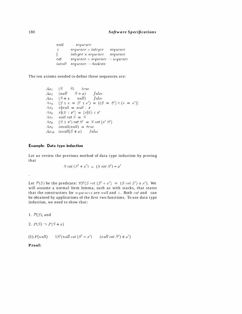
180 Software Specifications
null � sequence� sequence � integer � sequencej integer � sequence� sequencecat sequence � sequence� sequenceisnull sequence� boolean
The ten axioms needed to define these sequences are:
Ax1 �S � S� � trueAx2 �null � S � x� � falseAx3 �S � x � null� � falseAx4 �S � x � S� � x�� � ��S � S�� �x � x���Ax5 xjnull � null � xAx6 xj�S � x�� � �xjS� � x�
Ax7 null cat S � SAx8 �S � x�� cat S� � S cat �x�jS��Ax9 isnull�null� � trueAx10 isnull�S � x� � false
Example� Data type induction
Let us review the previous method of data type induction by provingthat
S cat �S� � x�� � �S cat S�� � x�
.
Let P �S� be the predicate: �S��S cat �S� � x�� � �S cat S�� � x��. Wewill assume a normal form lemma, such as with stacks, that statesthat the constructors for sequences are null and �. Both cat and j canbe obtained by applications of the first two functions. To use data typeinduction, we need to show that:
1. P �S�, and
2. P �S� P �S � x�
(1) P �null� � �S��null cat �S� � x�� � �null cat S�� � x��
Proof:
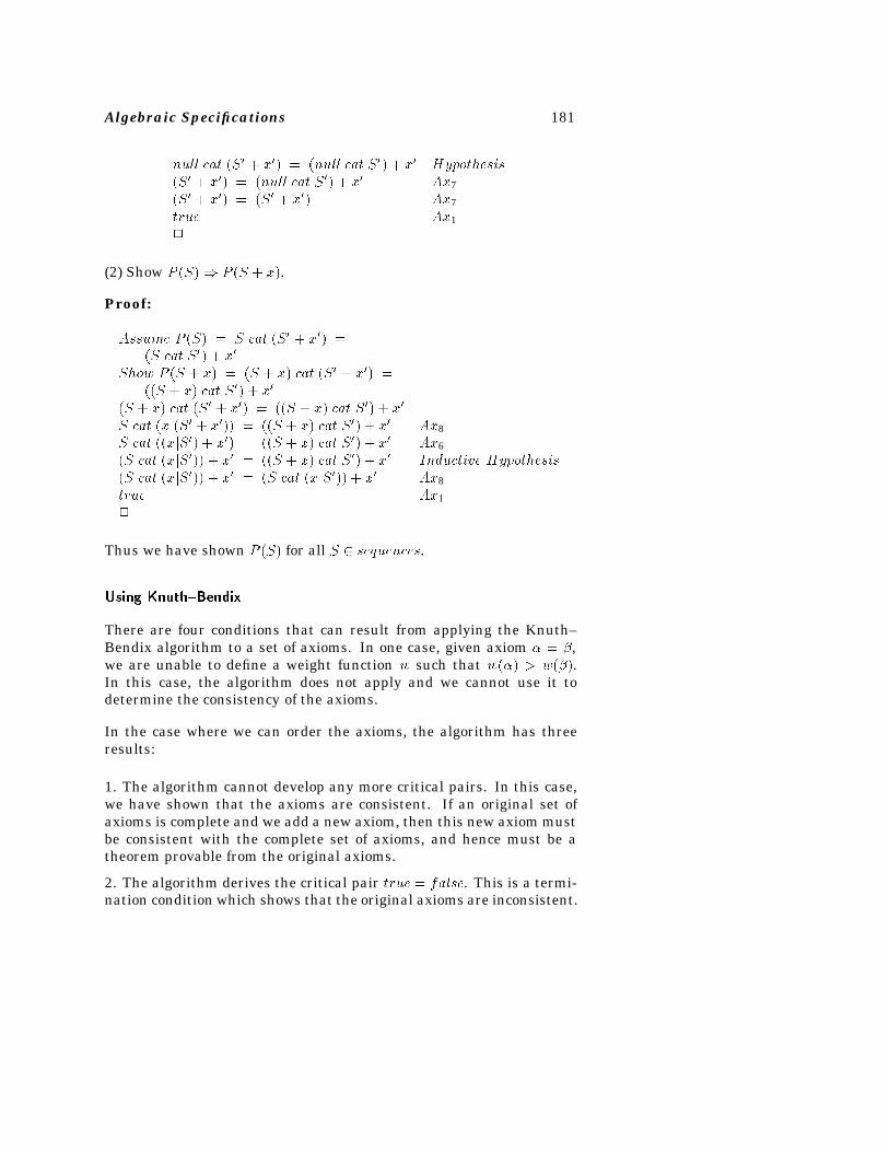
Algebraic Specifications 181
null cat �S� � x�� � �null cat S�� � x� Hypothesis�S� � x�� � �null cat S�� � x� Ax7�S� � x�� � �S� � x�� Ax7true Ax1�
(2) Show P �S� P �S � x�.
Proof:
Assume P �S� � S cat �S� � x�� ��S cat S�� � x�
Show P �S � x� � �S � x� cat �S� � x�� ���S � x� cat S�� � x�
�S � x� cat �S� � x�� � ��S � x� cat S�� � x�
S cat �xj�S� � x��� � ��S � x� cat S�� � x� Ax8S cat ��xjS�� � x�� � ��S � x� cat S�� � x� Ax6�S cat �xjS��� � x� � ��S � x� cat S�� � x� Inductive Hypothesis�S cat �xjS��� � x� � �S cat �xjS��� � x� Ax8true Ax1�
Thus we have shown P �S� for all S � sequences.
Using Knuth�Bendix
There are four conditions that can result from applying the Knuth–Bendix algorithm to a set of axioms. In one case, given axiom � � �,we are unable to define a weight function w such that w��� � w���.In this case, the algorithm does not apply and we cannot use it todetermine the consistency of the axioms.
In the case where we can order the axioms, the algorithm has threeresults:
1. The algorithm cannot develop any more critical pairs. In this case,we have shown that the axioms are consistent. If an original set ofaxioms is complete and we add a new axiom, then this new axiom mustbe consistent with the complete set of axioms, and hence must be atheorem provable from the original axioms.
2. The algorithm derives the critical pair true � false. This is a termi-nation condition which shows that the original axioms are inconsistent.
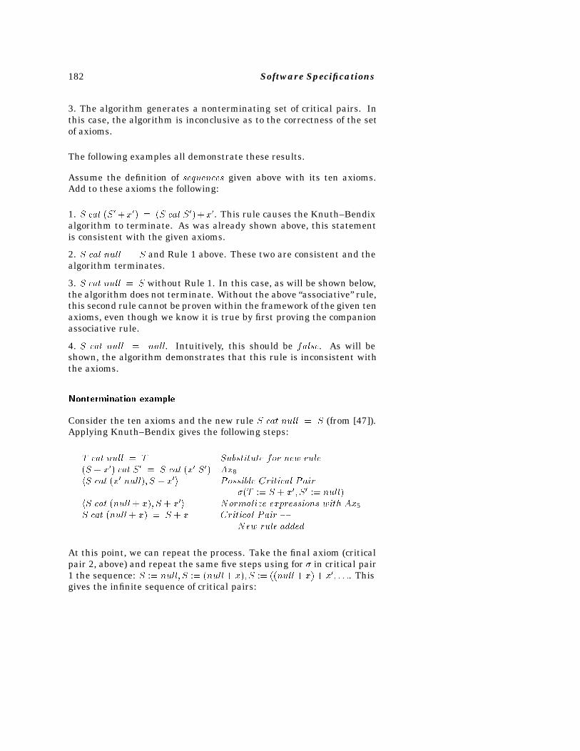
182 Software Specifications
3. The algorithm generates a nonterminating set of critical pairs. Inthis case, the algorithm is inconclusive as to the correctness of the setof axioms.
The following examples all demonstrate these results.
Assume the definition of sequences given above with its ten axioms.Add to these axioms the following:
1. S cat �S��x�� � �S cat S���x�. This rule causes the Knuth–Bendixalgorithm to terminate. As was already shown above, this statementis consistent with the given axioms.
2. S cat null � S and Rule 1 above. These two are consistent and thealgorithm terminates.
3. S cat null � S without Rule 1. In this case, as will be shown below,the algorithm does not terminate. Without the above “associative” rule,this second rule cannot be proven within the framework of the given tenaxioms, even though we know it is true by first proving the companionassociative rule.
4. S cat null � null. Intuitively, this should be false. As will beshown, the algorithm demonstrates that this rule is inconsistent withthe axioms.
Nontermination example
Consider the ten axioms and the new rule S cat null � S (from [47]).Applying Knuth–Bendix gives the following steps:
T cat null � T Substitute for new rule�S � x�� cat S� � S cat �x�jS�� Ax8hS cat �x�jnull�� S � x�i Possible Critical Pair
��T :� S � x�� S� :� null�hS cat �null � x�� S � x�i Normalize expressions with Ax5S cat �null � x� � S � x Critical Pair �
New rule added
At this point, we can repeat the process. Take the final axiom (criticalpair 2, above) and repeat the same five steps using for � in critical pair1 the sequence: S :� null� S :� �null� x�� S :� ��null � x� � x�� � � �. Thisgives the infinite sequence of critical pairs:
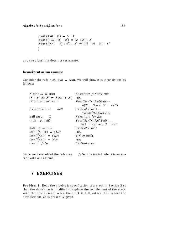
Algebraic Specifications 183
S cat �null � x�� � S � x�
S cat ��null � x� � x�� � �S � x� � x�
S cat ���null � x� � x�� � x�� � ��S � x� � x�� � x��
...
and the algorithm does not terminate.
Inconsistent axiom example
Consider the rule S cat null � null. We will show it is inconsistent asfollows:
T cat null � null Substitute for new rule�S � x�� cat S� � S cat �x�jS�� Ax8hS cat �x�jnull�� nulli Possible CriticalPair�
��T :� S � x�� S� :� null�S cat �null � x� � null Critical Pair 1�
Normalize with Ax5null cat T � T Substitute for Ax7hnull � x� nulli Possible Critical Pair�
��T :� null � x� S :� null�null � x � null Critical Pair 2isnull�S � x� � false Ax10isnull�null� � false ��S :� null�isnull�null� � true Ax9true � false Critical Pair
Since we have added the rule true � false, the initial rule is inconsis-tent with our axioms.
�� EXERCISES
Problem 1. Redo the algebraic specification of a stack in Section 3 sothat the definition is modified to replace the top element of the stackwith the new element when the stack is full, rather than ignore thenew element, as is presently given.
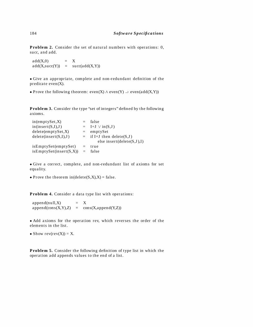
184 Software Specifications
Problem 2. Consider the set of natural numbers with operations: 0,succ, and add.
add(X,0) = Xadd(X,succ(Y)) = succ(add(X,Y))
� Give an appropriate, complete and non-redundant definition of thepredicate even(X).
� Prove the following theorem: even(X) even(Y) even(add(X,Y))
Problem 3. Consider the type “set of integers” defined by the followingaxioms.
in(emptySet,X) = falsein(insert(S,I),J) = I=J � in(S,J)delete(emptySet,X) = emptySetdelete(insert(S,I),J) = if I=J then delete(S,J)
else insert(delete(S,J),I)isEmptySet(emptySet) = trueisEmptySet(insert(S,X)) = false
� Give a correct, complete, and non-redundant list of axioms for setequality.
� Prove the theorem in(delete(S,X),X) = false.
Problem 4. Consider a data type list with operations:
append(null,X) = Xappend(cons(X,Y),Z) = cons(X,append(Y,Z))
� Add axioms for the operation rev, which reverses the order of theelements in the list.
� Show rev(rev(X)) = X.
Problem 5. Consider the following definition of type list in which theoperation add appends values to the end of a list.
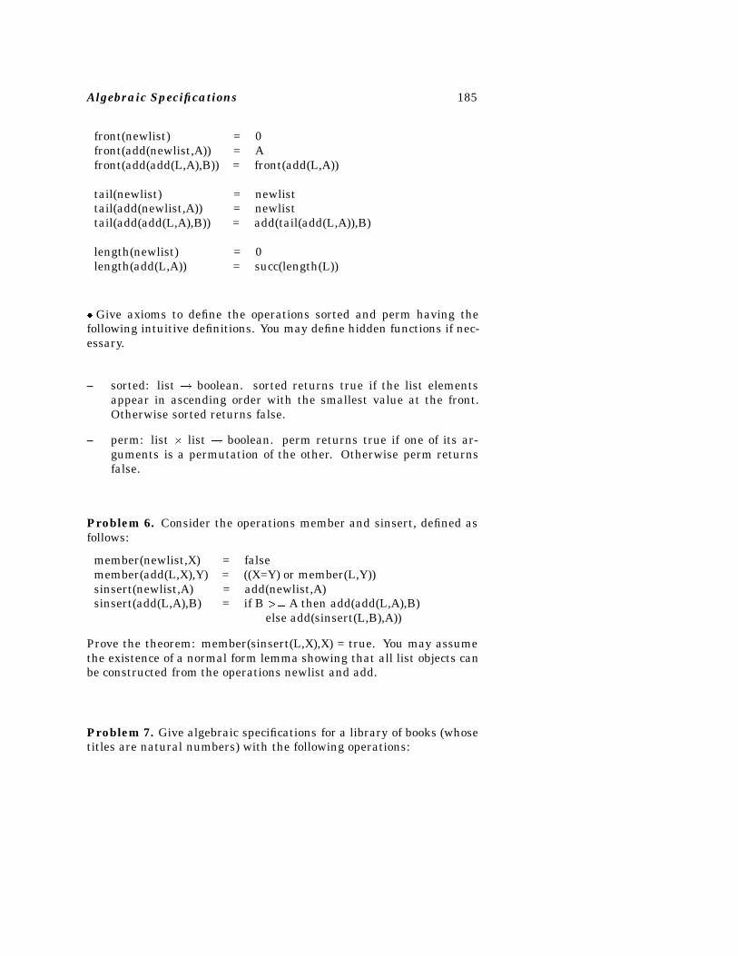
Algebraic Specifications 185
front(newlist) = 0front(add(newlist,A)) = Afront(add(add(L,A),B)) = front(add(L,A))
tail(newlist) = newlisttail(add(newlist,A)) = newlisttail(add(add(L,A),B)) = add(tail(add(L,A)),B)
length(newlist) = 0length(add(L,A)) = succ(length(L))
� Give axioms to define the operations sorted and perm having thefollowing intuitive definitions. You may define hidden functions if nec-essary.
– sorted: list � boolean. sorted returns true if the list elementsappear in ascending order with the smallest value at the front.Otherwise sorted returns false.
– perm: list � list � boolean. perm returns true if one of its ar-guments is a permutation of the other. Otherwise perm returnsfalse.
Problem 6. Consider the operations member and sinsert, defined asfollows:
member(newlist,X) = falsemember(add(L,X),Y) = ((X=Y) or member(L,Y))sinsert(newlist,A) = add(newlist,A)sinsert(add(L,A),B) = if B �� A then add(add(L,A),B)
else add(sinsert(L,B),A))
Prove the theorem: member(sinsert(L,X),X) = true. You may assumethe existence of a normal form lemma showing that all list objects canbe constructed from the operations newlist and add.
Problem 7. Give algebraic specifications for a library of books (whosetitles are natural numbers) with the following operations:
186 Software Specifications
init: � library open for businessdonate: library � nat � library add a volume to libraryremove: library � nat � library destroy a book & forget
it was donatedcheck: library � nat � library borrow a bookreturn: library � nat � library bring a book backgiven: library � nat � bool has a book been donated?avail: library � nat � bool is book available for checkout?out: library � nat � bool is book already checked out?
Using data type induction, show: given(L,B) � (avail(L,B) � out(L,B)).
Problem 8. The low-water-mark problem is defined for a system com-posed of processes and objects, each with its own security level. Threesecurity levels are linearly ordered: classified � secret � topsecret.Processes have fixed security levels, but objects’ security levels may bechanged by operations. When a process writes a value in an object, thesecurity level of the object drops to that of the process. When a processresets an object, the security level of the object becomes top secret andits value becomes undefined. The low-water-mark idea is that the se-curity level of an object may decrease, but not increase unless a resetoperation is executed for the object.
The Bell and LaPadula simple security and * properties (colloquiallyknown as “no read up, no write down”) require enforcement of thefollowing restrictions:
� For a process to read an object’s value, the security level of the processmust be greater than or equal to that of the object.
� For a process to write an object’s value, the security level of the processmust be less than or equal to that of the object.
Using the following operations, give an algebraic specification for thedata type state which enforces the Bell and LaPadula properties. Op-erations attempting to “read up” should return the undefined value.Operations attempting to “write down” should be ignored. Reset oper-ations enforce the same security-level restrictions as write operations.
Algebraic Specifications 187
newstate: � statereset: process � object � state � statewrite: process � object � nat � state � stateread: process � object � state � nat � fundefi nedgname: object � idlevel: object � state � (classified, secret, topsecret)level: process � (classified, secret, topsecret)
Problem 9. Consider the list data type with operations:
newlist : � listaddelt : list � nat� listtail : list� listhead : list� natlast : list� natlength : list� nat
with their usual meanings. Give three different sets of axioms defininglists in which elements are added to the right end of the list, in whichelements are added to the left end of the list, and in which elementsare added so that the list remains sorted in ascending order. To makethings a bit easier, you may define operations so that applying them toempty lists yields 0.
Problem 10. If we added the operation join to lists in which elementsare added to the right end of the list, we might write the axioms:
Signature :join : list � list� list
Axioms :join1 : join�L� newlist� � Ljoin2 : join�L� addelt�M�X�� � addelt�join�L�M �� X�
Show that join�newlist� L� � L is not an axiom, but a theorem followingfrom the given axioms.
Problem 11. Consider the following implementation of the data typeSetType with operations NewSet, AddElt, and Member. Give a repre-
188 Software Specifications
sentation function for the type and write comments for each operationgiving pre, post, in and out.
constSetMax = 256;
typeEltType = integer;SetIndex = 1..SetMax;SetType = record
Next: 0..SetMax;V: array [SetIndex] of EltType
end;
procedure NewSet(var S: SetType);begin
S.Next := 0end;
procedure AddElt(var S: SetType; E: EltType);var i: integer;begin
S.V[S.Next+1] := E;i := 1;while (i<=S.Next+1) and (S.V[i]<>E) do i := i+1;if i = S.Next+1 then S.Next := S.Next+1
end;
function Member(var S: SetType; E: EltType): boolean;var I: SetIndex;
B: boolean;begin
B := false;for I := 1 to S.Next do B := B or (E = S.V[I]);Member := B
end;
Problem 12. A bag or multiset is a set that permits duplicate values.Consider the following implementation of the data type “bag of inte-gers.” A set cannot be used to represent a bag, as there is no way toindicate the presence in a set of more than one occurrence of an ele-ment. Two good choices would be to represent a bag as a sequence of
Algebraic Specifications 189
elements, since a sequence can contain duplicated elements, or a setof pairs representing (element, number of occurrences). Which choicemakes the specification task easier?
const Max = ...;type T = integer;
Bag = array [0..Max] of T;procedure BagInit(var B: Bag);
var i: integer;begin
for i := 0 to Max do B[i] := 0end;
procedure BagAdd(var B: Bag; X: T);begin
if (0 <= X) and (X <= Max) then B[X] := B[X] + 1end;
procedure BagDel(var B: Bag; X: T);begin
if (0 <= X) and (X <= Max) and (B[X] > 0)then B[X] := B[X] - 1
end;function BagMember(var B: Bag; X: T): boolean;
beginif (0<=X) and (X<=Max) then BagMember := B[X]>0else BagMember := false
end;
Problem 13. Give a representation function for the type and abstractand concrete comments for data type IntSet.
type IntSet = array [1..Max] of boolean;
procedure IntSetInit(var S: IntSet);var i: integer;begin
for i := 1 to Max do S[i] := falseend;
procedure IntSetAdd(var S: IntSet; X: integer);begin
if (1<=X) and (X<=Max) then S[X] := true
190 Software Specifications
end
Problem 14. The following code implements type “queue of EltType”as a circular list with a contiguous representation.
const Max = 2;type
EltType = 0..maxint;QueueIndex = 0..Max;Queue = record
M: array [QueueIndex] of EltType;H, T: QueueIndex
end;
procedure NewQ(var Q: Queue);begin
Q.H := 0; Q.T := 0;end;
procedure EnQ(var Q: Queue; Elt: EltType);var Temp: QueueIndex;begin
Temp := (Q.T + 1) mod (Max + 1);if Temp <> Q.H then begin
Q.T := Temp;Q.M[Q.T] := Eltend;
end;
procedure DeQ(var Q: Queue; var Result: EltType);begin
if Q.H <> Q.T then beginQ.H := (Q.H + 1) mod (Max + 1);Result := Q.M[Q.H];end
else Result := 0end;
State a representation function for the type. State non-trivial con-crete and abstract invariants for the type and show that the concrete
Algebraic Specifications 191
invariant implies the abstract invariant. Give pre, post, in, and outcomments for NewQ and demonstrate their consistency.
�� SUGGESTED READINGS
The algebraic specification techniques are well-described in the papers:
� J. V. Guttag and J. J. Horning, “The algebraic specification of abstractdata types,” Acta Informatica, Vol. 10, 1978, pp. 27-52.
� J. V. Guttag, “Notes on Type Abstraction (Version 2),” IEEE Transac-tions on Software Engineering, Vol. 6, No. 1, 1980, pp. 13-23.
� J. V. Guttag, E. Horowitz, and D. R. Musser, “Abstract Data Typesand Software Validation ,” Communications of the ACM, Vol. 21, No.12, 1978, pp. 1048-1064.
� J. V. Guttag, E. Horowitz, and D.R. Musser, “The Design of DataType Specifications ,” R.T. Yeh (Ed.), Current Trends in ProgrammingMethodology 4: Data Structuring, Prentice-Hall, Englewood Cliffs NJ,1978, pp. 60-79.
A paper which summarizes the verification process for algebraicallyspecified data types is the following. This paper presents a straightfor-ward technique for expressing algebraic axioms as a pair of pre- andpostconditions suitable for Hoare-style proofs.
� L. Flon and J. Misra, “A Unified Approach to the Specification andVerification of Abstract Data Types,” Proceedings of the IEEE Con-ference on Specifications of Reliable Software, Cambridge, MA, 1979,pp. 162-169.
Papers which describe proof techniques for algebraic data types includethe following:
� D. R. Musser, “Abstract data type specifications in the AFFIRM sys-tem,” IEEE Specifications of Reliable Software Conference, CambridgeMA, 1979, pp. 47-57.
192 Software Specifications
� D. R. Musser, “On Proving Inductive Properties of Abstract DataTypes,” Proceedings of the 7th ACM Symposium on Principles of Pro-gramming Languages, Las Vegas, NV, 1980, pp. 154-162.
� G. Huet, “Confluent Reductions: Abstract Properties and Applica-tions to Term-Rewriting Systems,” Journal of the ACM, Vol. 27, 1980,pp. 797-821.
� G. Huet and J.-M. Hullot, “Proofs by Induction in Equational Theorieswith Constructors ,” Journal of Computer and System Science, Vol. 25,1982, pp. 239-266.
The first two Musser papers describe the application of the Knuth–Bendix algorithm to the problem of proving properties of ADTs – inthis case by describing the AFFIRM system, which Musser built.
Chapter 6
Denotational Semantics
Denotational semantics is a form of an operational semantic model of aprogram’s execution based upon function composition. The basic modelis an outgrowth of simple type theory and the �calculus. First the�calculus will be described, and then denotational semantics will beexplained as an extension.
Aside from its role in explaining semantic content of a program, the�calculus is the basis for the VDM specification methodology, whichhas been used to specify several very large real systems.
�� THE LAMBDA CALCULUS
The �calculus is a formal functional model used by Church to developa theory of numbers. It is relevant to programming language designsince it represents a typeless (hence simpler) model in the theory ofdenotational semantics.
�expressions are defined recursively as:
1. If x is a variable name, then x is a �expression.
2. If M is a �-expression, then �xM is a �expression.
193
194 Software Specifications
3. If F and A are �expressions, then �FA� is a �expression. F is theoperator and A is the operand.
The following are all �expressions:
x �xx �xy�x�xy� ��x�xx��x�xx�� �x�yx
Variables may be bound or free. In �xM , x is the binding variable andoccurrences of x in M are bound. A variable is free if it is not bound.
Any bound variable may have its name changed. Thus the �expression�xx is equivalent to�yy. �x�xx is equivalent to�x�yy since the variablex is not free in the original �expression �xx.
Informally, bound variables are “parameters” to the function describedby the �expression, free variables are global. There is no concept oflocal variable.
This analogy shows that the �expression is a simple approximation tothe procedure or subroutine concept in most algorithmic programminglanguages like Pascal, C, Ada or Fortran. �expressions are almostdirectly representable in LISP and �substitutions are a direct model ofAlgol-like procedures.
�expressions have only one operation – reduction. If �FA� is a �expres-sion, and F � �xM , then A may be substituted for all free occurrencesof x in M . This is written as: ��xMA� � F �.
Examples:
��xxy� � y��x�xy�y� � �yy���x�xy��xx� � ��xxy� � y��x�xx��x�xx�� � ��x�xx��x�xx�� � � � �
Note that the above examples are all unambiguous. The first expres-sion ��xxy� has only one interpretation. It must be of the form �F A�or ��xM A�. So A is either y or xy. But xy is not a proper �expression,so A is just y.
Denotational Semantics 195
Also note that the third expression does not terminate. If we haveF � ��xM A�, substitution of A for x in M results in F again. This is anonterminating reduction. This leads us to:
Church-Rosser property. If two different reductions of a �expressionterminate, then they are members of the same value class.
The �calculus was originally developed as a logical model of the com-putational process. We can use such expressions to model our under-standing of arithmetic. First �expressions will be used to model thepredicate calculus, and then using predicate calculus, we can modelintegers.
���� Boolean Values as �Expressions
Objects will be modeled by functions.
True T will be defined as: �x�yx. (Of a pair, choose the first.)
False F will be defined as: �x�yy. (Of a pair, choose the second.)
We have defined these objects so the following properties are true:
��T P �Q� � P
Proof:
��T P �Q� � ���x�yx P �Q� � ��yP Q�� P
�
��F P �Q� � Q
Proof:
��F P �Q� � ���x�yy P �Q�� ��yy Q�� Q
�
Given these constants T and F , we can define the boolean function:
not�� �x��xF �T �
196 Software Specifications
Given these definitions, we need to show that our interpretation ofthem is consistent with our axioms and rules of predicate logic. In thiscase, we need to show that not, when applied to T returns F , and notwhen applied to F returns T .
�not T � � ��x��x F �T �T � � ��T F �T � � F�not F � � ��x��x F �T �F � � ��F F �T � � T
Note that this is the desired behavior. Nothing is said if the argumentto not is neither T nor F .
Similarly, we can define and and or as:
and�� �x�y��xy�F �
or�� �x�y��xT �y�
���� Integers
From these logical functions, we can now develop the integers:
0 �� �f�cc
1 �� �f�c�fc�
2�� �f�c�f�fc��
3�� �f�c�f�f�fc���
c plays the role of the “zero” element, and f is the “successor” function(addition of �1).
From these definitions of the integers, we can extend them to includeour usual arithmetic operations.
Let N be the Nth integer. The �expression �N a� is �c�a � � � �a c� � � ��.Computing ��N a�b�, we get �a � � � �a b� � � ��.
Consider ��M a���N a�b�� by applying constant ��N a�b� to �expression�M a�. The substitution of ��N a�b� for c in �M a� yields �a � � � �a b� � � ��where there are now �M � N � as in the list. We have just developedaddition. Therefore:
Addition:
Denotational Semantics 197
�M �N ��� �a�b��M a���N a�b��
��� �M�N�a�b��M a���N a�b��
Similarly,
Multiplication:�M � N �
�� �a�M �N a��
Exponentiation:�MN �
�� �N M �
While this development can continue until we have developed all of therecursive functions of mathematics, our primary goal is to consider thesemantics of programming languages. So we will leave the �calculusat this point and start to look at datatypes.
�� Datatypes
�expressions either reduce to constants (value) or to other �expressions.Thus all �expressions are solutions to the functional equation:
value � constant � �value � value�
But there exists no set solving this, since the cardinality of functionsfrom �value � value� is greater than the cardinality of values.
Assume we have infinite objects with some finite approximation as arepresentation. Object a approximates object b (written a ap b) if b is atleast as accurate as a.
Examples:
1. aapb if whenever a is defined, b is defined and gives the same answer.
2. Let �x1� x2� be a line interval. �x1� x2� ap �y1� y2� if x1 � y1 � y2 � x2.That is �y1� y2� is contained in �x1� x2�.
Axiom 1: A datatype is a partially ordered set according to relation ap.
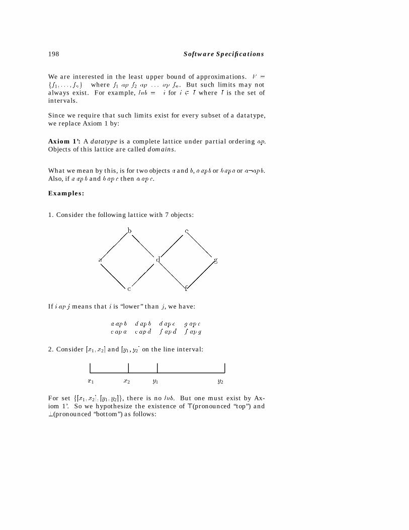
198 Software Specifications
We are interested in the least upper bound of approximations. F �ff1� � � � � fng where f1 ap f2 ap � � � ap fn. But such limits may notalways exist. For example, lub � �i for i � I where I is the set ofintervals.
Since we require that such limits exist for every subset of a datatype,we replace Axiom 1 by:
Axiom 1’: A datatype is a complete lattice under partial ordering ap.Objects of this lattice are called domains.
What we mean by this, is for two objects a and b, aapb or bapa or a�apb.Also, if a ap b and b ap c then a ap c.
Examples:
1. Consider the following lattice with 7 objects:
��
��
�����
���
�����
���
��
��
����
����
c
g
f
e
d
b
a
If i ap j means that i is “lower” than j, we have:
a ap b d ap b d ap e g ap ec ap a c ap d f ap d f ap g
2. Consider �x1� x2� and �y1� y2� on the line interval:
y2y1x2x1
For set f�x1� x2�� �y1� y2�g, there is no lub. But one must exist by Ax-iom 1’. So we hypothesize the existence of �(pronounced “top”) and�(pronounced “bottom”) as follows:
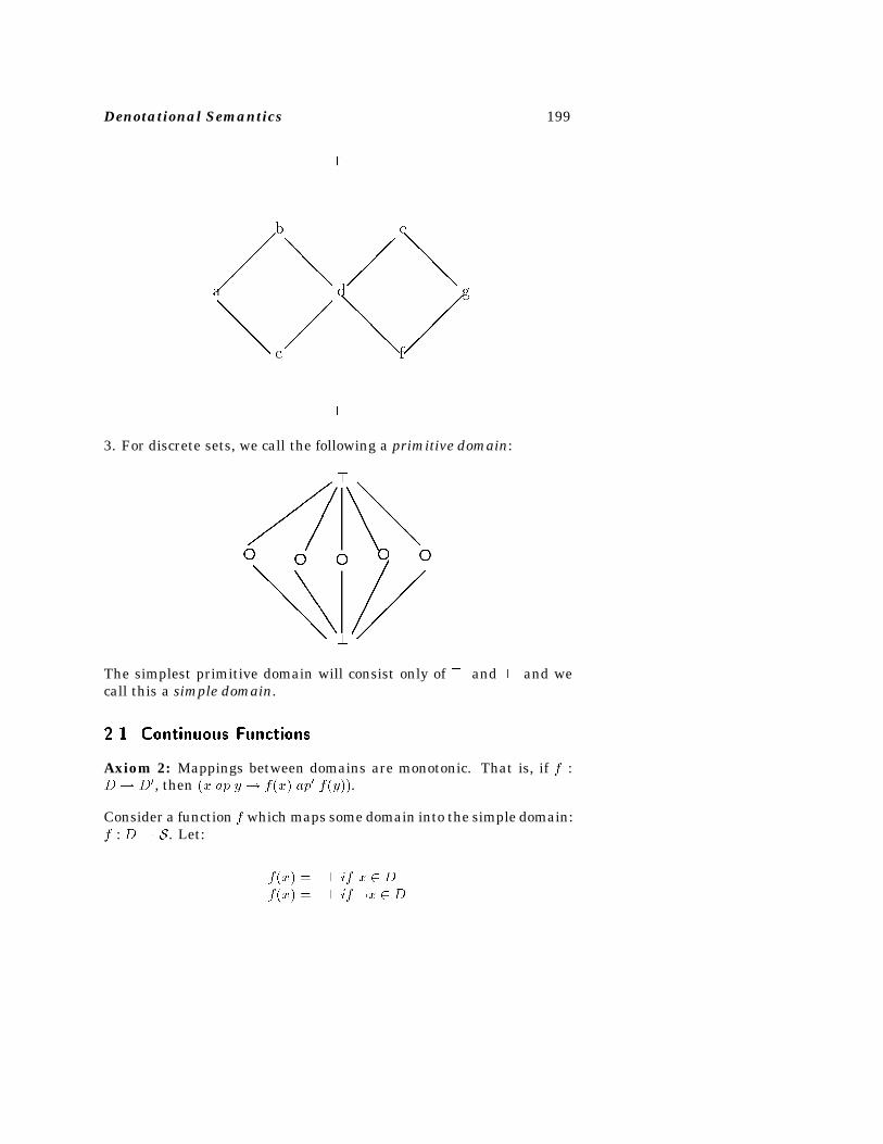
Denotational Semantics 199
��������
� � � � � � �
����
����
�
� �� �� �� �� �
��
��
�����
���
�����
���
��
��
����
����
�
�
c
g
f
e
d
b
a
3. For discrete sets, we call the following a primitive domain:
fffff
�����
�����
��
��
��
AAAAA
JJJJJ
�
�
The simplest primitive domain will consist only of � and � and wecall this a simple domain.
���� Continuous Functions
Axiom 2: Mappings between domains are monotonic. That is, if f :D � D�, then �x ap y � f�x� ap� f�y��.
Consider a function f which maps some domain into the simple domain:f : D � S. Let:
f�x� � � if x � Df�x� � � if �x � D
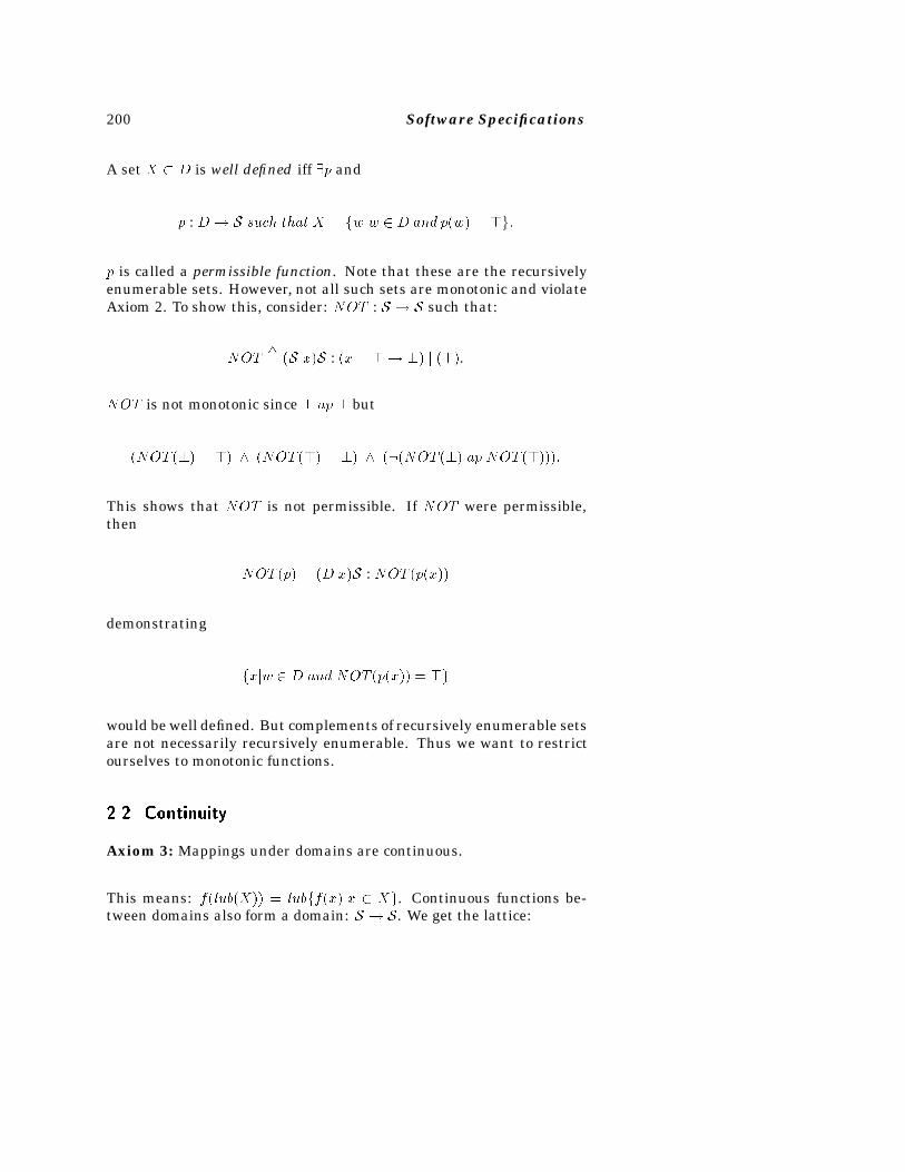
200 Software Specifications
A set X � D is well defined iff �p and
p : D � S such that X � fwjw � D and p�w� � �g�
p is called a permissible function. Note that these are the recursivelyenumerable sets. However, not all such sets are monotonic and violateAxiom 2. To show this, consider: NOT : S � S such that:
NOT�� �S x�S : �x � �� �� j ���.
NOT is not monotonic since � ap � but
�NOT ��� � �� �NOT ��� � �� ���NOT ��� ap NOT ������
This shows that NOT is not permissible. If NOT were permissible,then
NOT �p� � �D x�S : NOT �p�x��
demonstrating
fxjw � D and NOT �p�x�� � �g
would be well defined. But complements of recursively enumerable setsare not necessarily recursively enumerable. Thus we want to restrictourselves to monotonic functions.
���� Continuity
Axiom 3: Mappings under domains are continuous.
This means: f�lub�X�� � lubff�x�jx � Xg. Continuous functions be-tween domains also form a domain: S � S. We get the lattice:
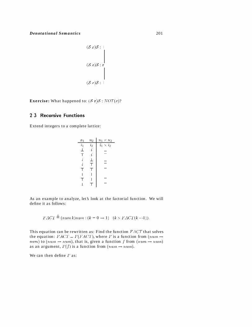
Denotational Semantics 201
�S x�S : �
�S x�S : x
�S x�S : �
Exercise: What happened to: �S x�S : NOT �x�?
���� Recursive Functions
Extend integers to a complete lattice:
n1 n2 n1 � n2
i1 i2 i1 � i2� i �� i �i � �i � �� � �� � �� � �� � �
As an example to analyze, let’s look at the factorial function. We willdefine it as follows:
FACT�� �num k�num : �k � 0 � 1� j �k � FACT �k � 1���
This equation can be rewritten as: Find the function FACT that solvesthe equation: FACT � F �FACT �, where F is a function from �num�num� to �num � num�, that is, given a function f from �num � num�as an argument, F �f� is a function from �num� num�.
We can then define F as:
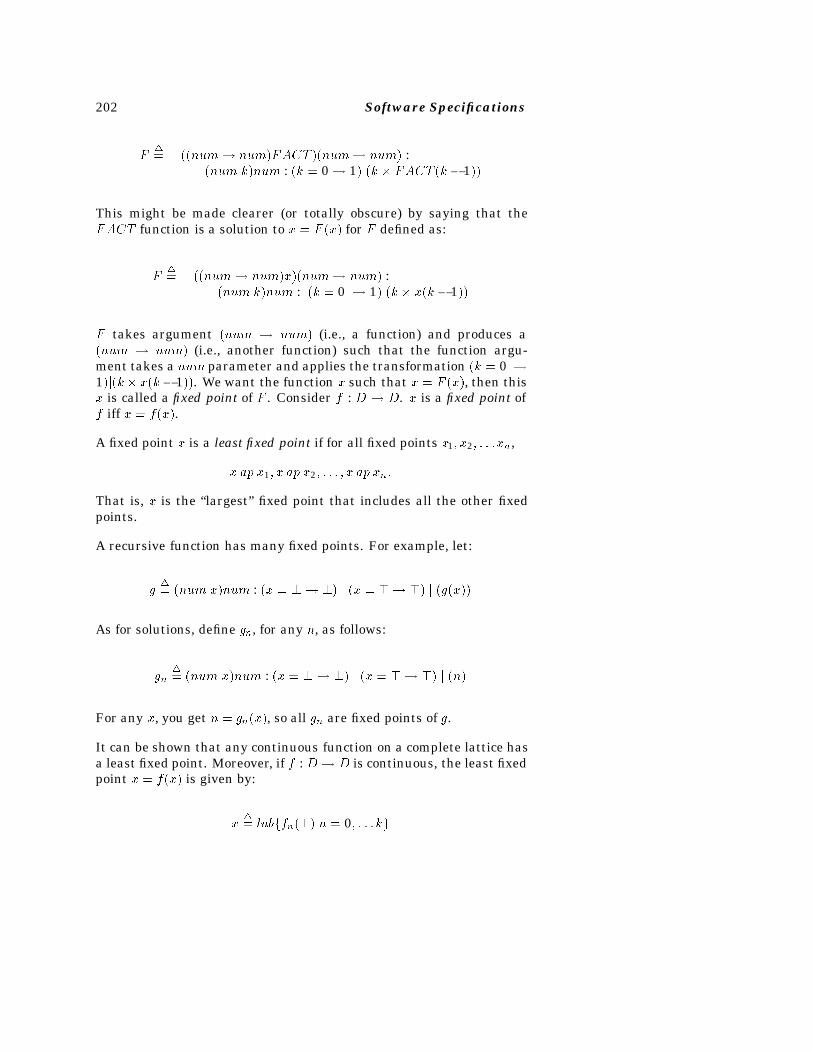
202 Software Specifications
F�� ��num� num�FACT ��num� num� :
�num k�num : �k � 0 � 1�j�k � FACT �k � 1��
This might be made clearer (or totally obscure) by saying that theFACT function is a solution to x � F �x� for F defined as:
F�� ��num� num�x��num� num� :
�num k�num : �k � 0 � 1�j�k � x�k � 1��
F takes argument �num � num� (i.e., a function) and produces a�num � num� (i.e., another function) such that the function argu-ment takes a num parameter and applies the transformation �k � 0 �1�j�k� x�k� 1��. We want the function x such that x � F �x�, then thisx is called a fixed point of F . Consider f : D � D. x is a fixed point off iff x � f�x�.
A fixed point x is a least fixed point if for all fixed points x1� x2� � � �xn,
x ap x1� x ap x2� � � � � x ap xn�
That is, x is the “largest” fixed point that includes all the other fixedpoints.
A recursive function has many fixed points. For example, let:
g�� �num x�num : �x � �� �� j �x � �� �� j �g�x��
As for solutions, define gn, for any n, as follows:
gn�� �num x�num : �x � �� �� j �x � �� �� j �n�
For any x, you get n � gn�x�, so all gn are fixed points of g.
It can be shown that any continuous function on a complete lattice hasa least fixed point. Moreover, if f : D � D is continuous, the least fixedpoint x � f�x� is given by:
x�� lubffn���jn � 0� � � �kg
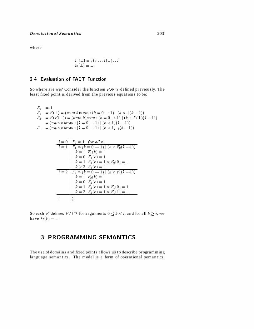
Denotational Semantics 203
where
fn��� � f�f � � � f��� � � ��f0��� � �
���� Evaluation of FACT Function
So where are we? Consider the function FACT defined previously. Theleast fixed point is derived from the previous equations to be:
F0 � �F1 � F ��� � �num k�num : �k � 0 � 1� j �k � ��k � 1��F2 � F �F ���� � �num k�num : �k � 0 � 1� j �k � F ����k � 1��
� �num k�num : �k � 0 � 1� j �k � F1�k � 1��Fi � �num k�num : �k � 0 � 1� j �k � Fi�1�k � 1��
i � 0 F0 � � for all ki � 1 F1 � �k � 0 � 1� j �k � F0�k � 1��
k � � F1�k� � �k � 0 F1�k� � 1k � 1 F1�k� � 1� F0�0� � �k � 2 F1�k� � �
i � 2 F2 � �k � 0 � 1� j �k � F1�k � 1��k � � F2�k� � �k � 0 F2�k� � 1k � 1 F2�k� � 1� F1�0� � 1k � 2 F2�k� � 1� F1�1� � �
......
So each Fi defines FACT for arguments 0 � k � i, and for all k � i, wehave Fi�k� � �.
�� PROGRAMMING SEMANTICS
The use of domains and fixed points allows us to describe programminglanguage semantics. The model is a form of operational semantics,
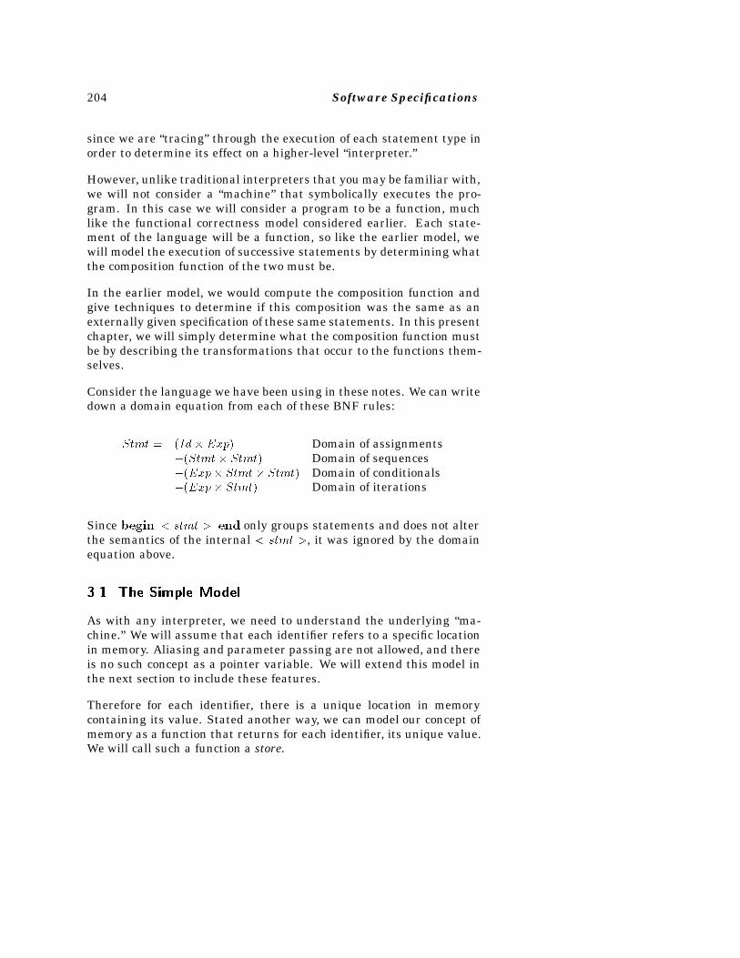
204 Software Specifications
since we are “tracing” through the execution of each statement type inorder to determine its effect on a higher-level “interpreter.”
However, unlike traditional interpreters that you may be familiar with,we will not consider a “machine” that symbolically executes the pro-gram. In this case we will consider a program to be a function, muchlike the functional correctness model considered earlier. Each state-ment of the language will be a function, so like the earlier model, wewill model the execution of successive statements by determining whatthe composition function of the two must be.
In the earlier model, we would compute the composition function andgive techniques to determine if this composition was the same as anexternally given specification of these same statements. In this presentchapter, we will simply determine what the composition function mustbe by describing the transformations that occur to the functions them-selves.
Consider the language we have been using in these notes. We can writedown a domain equation from each of these BNF rules:
Stmt � �Id� Exp� Domain of assignments��Stmt � Stmt� Domain of sequences��Exp� Stmt � Stmt� Domain of conditionals��Exp� Stmt� Domain of iterations
Since begin � stmt � end only groups statements and does not alterthe semantics of the internal � stmt �, it was ignored by the domainequation above.
���� The Simple Model
As with any interpreter, we need to understand the underlying “ma-chine.” We will assume that each identifier refers to a specific locationin memory. Aliasing and parameter passing are not allowed, and thereis no such concept as a pointer variable. We will extend this model inthe next section to include these features.
Therefore for each identifier, there is a unique location in memorycontaining its value. Stated another way, we can model our concept ofmemory as a function that returns for each identifier, its unique value.We will call such a function a store.
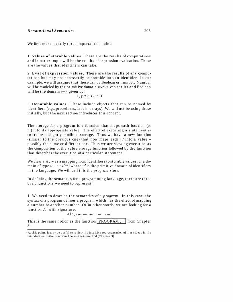
Denotational Semantics 205
We first must identify three important domains:
1. Values of storable values. These are the results of computationsand in our example will be the results of expression evaluation. Theseare the values that identifiers can take.
2. Eval of expression values. These are the results of any compu-tations but may not necessarily be storable into an identifier. In ourexample, we will assume that these can be Boolean or number. Numberwill be modeled by the primitive domain num given earlier and Booleanwill be the domain bool given by:
�� false� true��
3. Denotable values. These include objects that can be named byidentifiers (e.g., procedures, labels, arrays). We will not be using theseinitially, but the next section introduces this concept.
The storage for a program is a function that maps each location (orid) into its appropriate value. The effect of executing a statement isto create a slightly modified storage. Thus we have a new function(similar to the previous one) that now maps each id into a value –possibly the same or different one. Thus we are viewing execution asthe composition of the value storage function followed by the functionthat describes the execution of a particular statement.
We view a store as a mapping from identifiers to storable values, or a do-main of type id� value, where id is the primitive domain of identifiersin the language. We will call this the program state.
In defining the semantics for a programming language, there are threebasic functions we need to represent:1
1. We need to describe the semantics of a program. In this case, thesyntax of a program defines a program which has the effect of mappinga number to another number. Or in other words, we are looking for afunction M with signature:
M : prog � �num� num�
This is the same notion as the function PROGRAM � � � from Chapter3.
1At this point, it may be useful to review the intuitive representation of these ideas in theintroduction to the functional correctness method (Chapter 3).
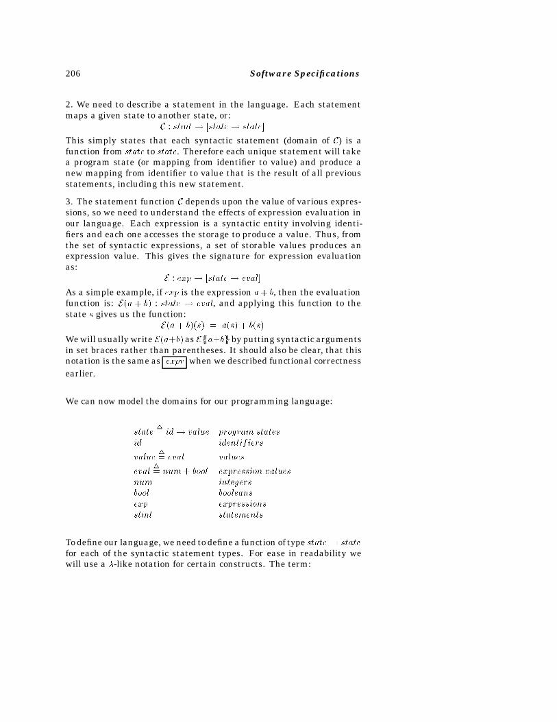
206 Software Specifications
2. We need to describe a statement in the language. Each statementmaps a given state to another state, or:
C : stmt � �state� state�
This simply states that each syntactic statement (domain of C) is afunction from state to state. Therefore each unique statement will takea program state (or mapping from identifier to value) and produce anew mapping from identifier to value that is the result of all previousstatements, including this new statement.
3. The statement function C depends upon the value of various expres-sions, so we need to understand the effects of expression evaluation inour language. Each expression is a syntactic entity involving identi-fiers and each one accesses the storage to produce a value. Thus, fromthe set of syntactic expressions, a set of storable values produces anexpression value. This gives the signature for expression evaluationas:
E : exp� �state� eval�
As a simple example, if exp is the expression a� b, then the evaluationfunction is: E�a � b� : state � eval, and applying this function to thestate s gives us the function:
E�a� b��s� � a�s� � b�s�
We will usually write E�a�b� as Effa�bggby putting syntactic argumentsin set braces rather than parentheses. It should also be clear, that thisnotation is the same as expr when we described functional correctnessearlier.
We can now model the domains for our programming language:
state�� id� value program states
id identifiers
value�� eval values
eval�� num� bool expression values
num integersbool booleansexp expressionsstmt statements
To define our language, we need to define a function of type state� statefor each of the syntactic statement types. For ease in readability wewill use a �-like notation for certain constructs. The term:
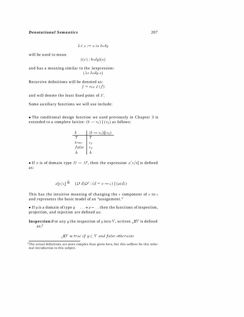
Denotational Semantics 207
let x :� a in body
will be used to mean��x� : body��a�
and has a meaning similar to the �expression:��x body a�
Recursive definitions will be denoted as:f � rec F �f�
and will denote the least fixed point of F .
Some auxiliary functions we will use include:
� The conditional design function we used previously in Chapter 3 isextended to a complete lattice: �b� v1� j �v2� as follows:
b �b� v1�j�v2�� �true v1false v2� �
� If x is of domain type D � D�, then the expression x�ve� is definedas:
x�ve��� �D d�D� : �d � v � e� j �x�d��
This has the intuitive meaning of changing the v component of x to eand represents the basic model of an “assignment.”
� If y is a domain of type y � � � ��x�� � � then the functions of inspection,projection, and injection are defined as:
Inspection:For any y the inspection of y into Y , written yEY is definedas:2
yEY � true if y � Y and false otherwise
2The actual definitions are more complex than given here, but this suffices for this infor-mal introduction to this subject.
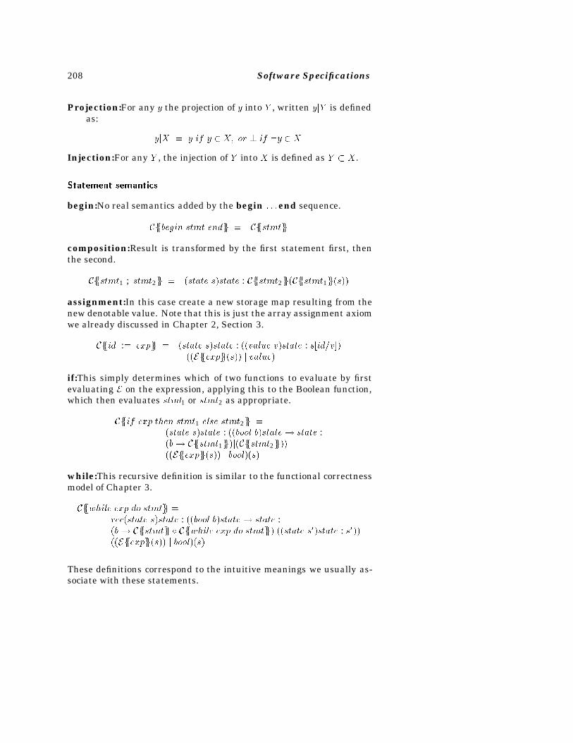
208 Software Specifications
Projection:For any y the projection of y into Y , written yjY is definedas:
yjX � y if y � X� or � if �y � X
Injection:For any Y , the injection of Y into X is defined as Y � X.
Statement semantics
begin:No real semantics added by the begin � � �end sequence.
Cffbegin stmt endgg � Cffstmtgg
composition:Result is transformed by the first statement first, thenthe second.
Cffstmt1 ; stmt2gg � �state s�state : Cffstmt2gg�Cffstmt1gg�s��
assignment:In this case create a new storage map resulting from thenew denotable value. Note that this is just the array assignment axiomwe already discussed in Chapter 2, Section 3.
Cffid :� expgg � �state s�state : ��value v�state : s�idv����Effexpgg�s�� j value�
if:This simply determines which of two functions to evaluate by firstevaluating E on the expression, applying this to the Boolean function,which then evaluates stmt1 or stmt2 as appropriate.
Cffif exp then stmt1 else stmt2gg ��state s�state : ��bool b�state� state :�b� Cffstmt1gg�j�Cffstmt2gg����Effexpgg�s�� j bool��s�
while:This recursive definition is similar to the functional correctnessmodel of Chapter 3.
Cffwhile exp do stmtgg �rec�state s�state : ��bool b�state� state :�b� Cffstmtgg Cffwhile exp do stmtgg�j��state s��state : s�����Effexpgg�s�� j bool��s�
These definitions correspond to the intuitive meanings we usually as-sociate with these statements.
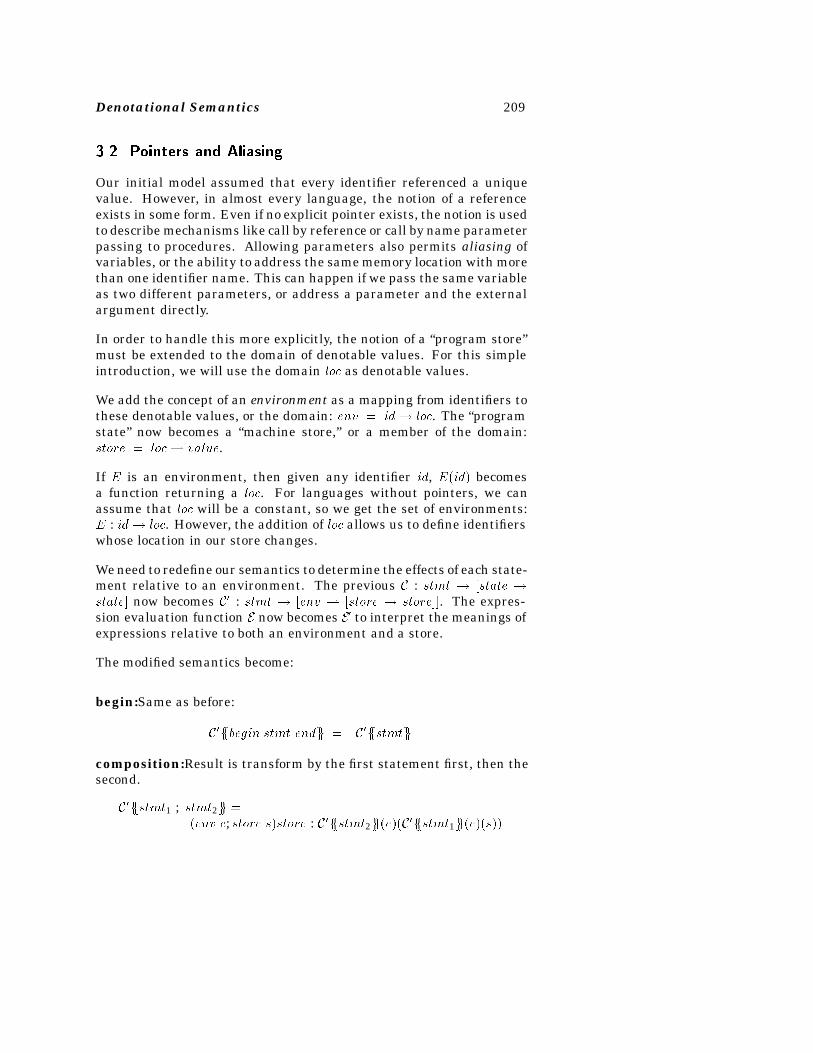
Denotational Semantics 209
���� Pointers and Aliasing
Our initial model assumed that every identifier referenced a uniquevalue. However, in almost every language, the notion of a referenceexists in some form. Even if no explicit pointer exists, the notion is usedto describe mechanisms like call by reference or call by name parameterpassing to procedures. Allowing parameters also permits aliasing ofvariables, or the ability to address the same memory location with morethan one identifier name. This can happen if we pass the same variableas two different parameters, or address a parameter and the externalargument directly.
In order to handle this more explicitly, the notion of a “program store”must be extended to the domain of denotable values. For this simpleintroduction, we will use the domain loc as denotable values.
We add the concept of an environment as a mapping from identifiers tothese denotable values, or the domain: env � id� loc. The “programstate” now becomes a “machine store,” or a member of the domain:store � loc� value.
If E is an environment, then given any identifier id, E�id� becomesa function returning a loc. For languages without pointers, we canassume that loc will be a constant, so we get the set of environments:E : id� loc. However, the addition of loc allows us to define identifierswhose location in our store changes.
We need to redefine our semantics to determine the effects of each state-ment relative to an environment. The previous C : stmt � �state �state� now becomes C� : stmt � �env � �store � store��. The expres-sion evaluation function E now becomes E� to interpret the meanings ofexpressions relative to both an environment and a store.
The modified semantics become:
begin:Same as before:
C�ffbegin stmt endgg � C�ffstmtgg
composition:Result is transform by the first statement first, then thesecond.
C�ffstmt1 ; stmt2gg ��env e; store s�store : C�ffstmt2gg�e��C�ffstmt1gg�e��s��
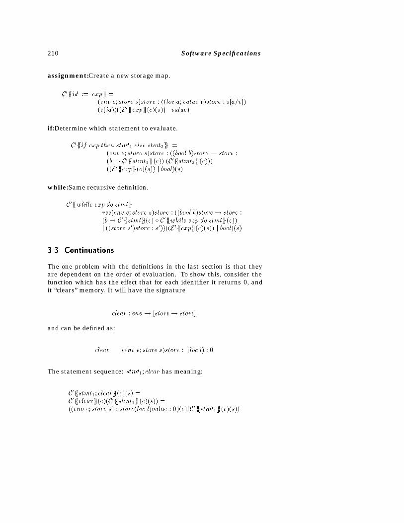
210 Software Specifications
assignment:Create a new storage map.
C�ffid :� expgg ��env e; store s�store : ��loc a; value v�store : s�av���e�id����E �ffexpgg�e��s�� j value�
if:Determine which statement to evaluate.
C�ffif exp then stmt1 else stmt2gg ��env e; store s�store : ��bool b�store � store :�b� C�ffstmt1gg�e��j�C�ffstmt2gg�e�����E �ffexpgg�e��s�� j bool��s�
while:Same recursive definition.
C�ffwhile exp do stmtgg �rec�env e; store s�store : ��bool b�store� store :�b� C�ffstmtgg�e� C�ffwhile exp do stmtgg�e��j ��store s��store : s�����E �ffexpgg�e��s�� j bool��s�
���� Continuations
The one problem with the definitions in the last section is that theyare dependent on the order of evaluation. To show this, consider thefunction which has the effect that for each identifier it returns 0, andit “clears” memory. It will have the signature
clear : env � �store� store�
and can be defined as:
clear � �env e; store s�store : �loc l� : 0
The statement sequence: stmt1; clear has meaning:
C�ffstmt1; cleargg�e��s� �C�ffcleargg�e��C�ffstmt1gg�e��s�� ���env e; store s� : store�loc l�value : 0��e��C �ffstmt1gg�e��s��
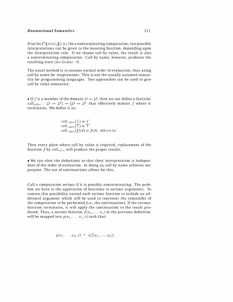
Denotational Semantics 211
If we let C�ffstmt1gg�e��s� be a nonterminating computation, two possibleinterpretations can be given to the meaning function, depending uponthe interpretation rule. If we choose call by value, the result is alsoa nonterminating computation. Call by name, however, produces theresulting store �loc l�value : 0.
The usual method is to assume normal order of evaluation, thus usingcall by name for �expressions. This is not the usually assumed seman-tics for programming languages. Two approaches can be used to givecall by value semantics:
� If f is a member of the domain D � D�, then we can define a functioncallvalue : �D � D�� � �D � D�� that effectively mimics f where itterminates. We define it as:
callvalue��� � ��
callvalue��� � ��
callvalue�f��d� � f�d�� otherwise
Then every place where call by value is required, replacement of thefunction f by callvalue will produce the proper results.
� We can alter the definitions so that their interpretation is indepen-dent of the order of evaluation. In doing so, call by name achieves ourpurpose. The use of continuations allows for this.
Call a computation serious if it is possibly nonterminating. The prob-lem we have is the application of functions to serious arguments. Toremove this possibility, extend each serious function to include an ad-ditional argument which will be used to represent the remainder ofthe computation to be performed (i.e., the continuation). If the seriousfunction terminates, it will apply the continuation to the result pro-duced. Thus, a serious function f�x1� � � � � xn� in the previous definitionwill be mapped into g�x1� � � � � xn� c� such that:
g�x1� � � � � xn� c� � c�f�x1� � � � � xn��
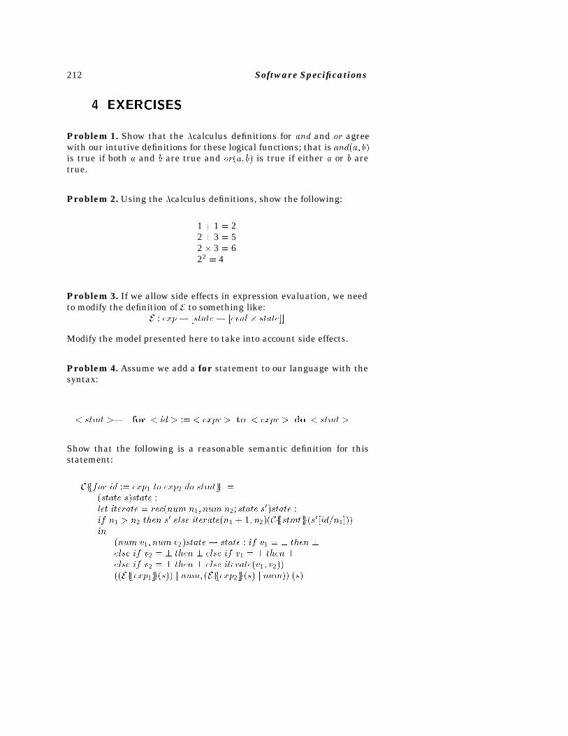
212 Software Specifications
�� EXERCISES
Problem 1. Show that the �calculus definitions for and and or agreewith our intutive definitions for these logical functions; that is and�a� b�is true if both a and b are true and or�a� b� is true if either a or b aretrue.
Problem 2. Using the �calculus definitions, show the following:
1 � 1 � 22 � 3 � 52� 3 � 622 � 4
Problem 3. If we allow side effects in expression evaluation, we needto modify the definition of E to something like:
E : exp� �state� �eval � state��
Modify the model presented here to take into account side effects.
Problem 4. Assume we add a for statement to our language with thesyntax:
� stmt �� for � id � :� � expr � to � expr � do � stmt �
Show that the following is a reasonable semantic definition for thisstatement:
Cfffor id :� exp1 to exp2 do stmtgg ��state s�state :let iterate � rec�num n1� num n2; state s��state :if n1 � n2 then s
� else iterate�n1 � 1� n2��Cffstmtgg�s��idn1���in
�num v1� num v2�state� state : if v1 � � then �else if v2 � � then � else if v1 � � then �else if v2 � � then � else iterate�v1� v2����Effexp1gg�s�� j num� �Effexp2gg�s� j num�� �s�
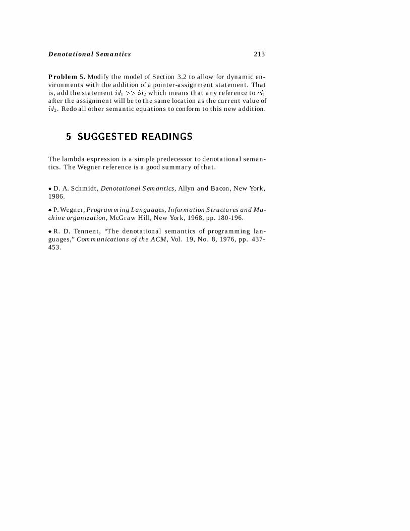
Denotational Semantics 213
Problem 5. Modify the model of Section 3.2 to allow for dynamic en-vironments with the addition of a pointer-assignment statement. Thatis, add the statement id1 �� id2 which means that any reference to id1after the assignment will be to the same location as the current value ofid2. Redo all other semantic equations to conform to this new addition.
�� SUGGESTED READINGS
The lambda expression is a simple predecessor to denotational seman-tics. The Wegner reference is a good summary of that.
� D. A. Schmidt, Denotational Semantics, Allyn and Bacon, New York,1986.
� P. Wegner, Programming Languages, Information Structures and Ma-chine organization, McGraw Hill, New York, 1968, pp. 180-196.
� R. D. Tennent, “The denotational semantics of programming lan-guages,” Communications of the ACM, Vol. 19, No. 8, 1976, pp. 437-453.

214 Software Specifications
Chapter 7
Specification Models
Previous chapters have described various notations for verifying that aprogram meets its specifications. However, most notations are hard toadapt to realistic programs. Here we look at approaches that attemptto model real programming issues, based upon the formal methods wealready discussed.
We will first describe VDM, a notation that uses many of the techniqueswe have already explained. We complete this chapter with a summaryof some recent results on risk analysis and evaluation of software spec-ifications.
�� VIENNA DEVELOPMENT METHOD
The IBM Vienna Laboratory developed a notation called the ViennaDevelopment Method (or VDM1). As we shall see, VDM adds very littlenew technology to what has already been described, except, perhaps,for an arcane notation. What VDM does do, however, is to pick andchoose from among the techniques we have studied, and to developa formalism and presentation that lends itself to realistic problems.VDM has a much wider following in Europe today, and is being usedfor many difficult programming tasks.
1VDM is not to be confused with the Vienna Definition Language, or VDL, which wasbriefly described earlier.
215
216 Software Specifications
While VDM was initially developed within IBM, the IBM group movedon to other topics and major development of the current model wasby Dines Bjorner of Lyngby, Denmark, who was concerned about sys-tems software specifications and by Cliff Jones in Manchester, UK, whowas concerned about VDM proof obligations and algorithm and datastructure refinement.
VDM contains the following features:
� The basic concept is to define a specification of a program, define asolution to that specification, and prove that the program meets thespecification.
� It is based upon denotational semantics and Mills’ functional correct-ness models in that it develops functions of the underlying program,and is concerned about transformations between program states.
� It permits formal proofs of program properties using a set of inferencerules, similar to the Hoare rules we studied earlier.
���� Overview of VDM
We present this short overview of VDM by describing the four basicfeatures in the method:
1. the underlying mathematical logic,
2. the definition of functions,
3. the definition of specifications, and
4. the method for verifying a function with its specification.
Underlying mathematical logic
VDM uses the predicate calculus for proving properties of specifica-tions. That means the mathematical theory presented earlier in Chap-ter 1, Section 5.4 forms the basis of the proof methodology. The sameset of rules of inference apply to this method as well as to the previouslydefined methods. VDM proofs look very similar to the Hoare axiomaticproofs we studied in Chapter 2.
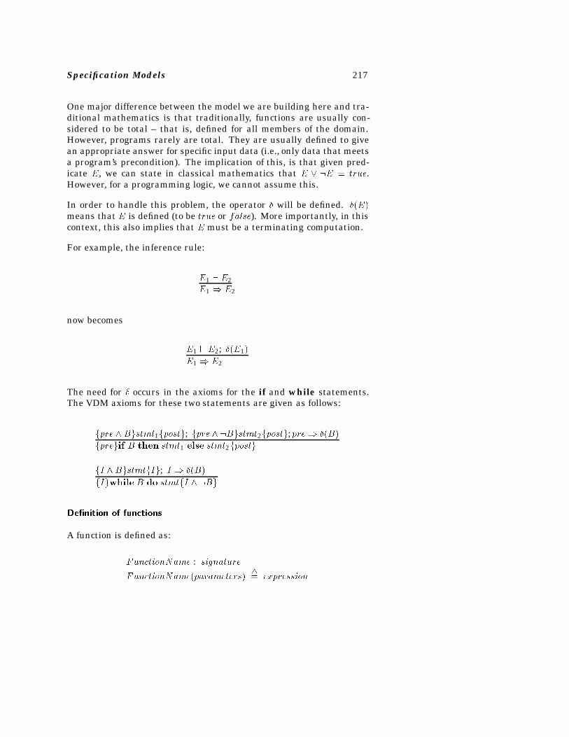
Specification Models 217
One major difference between the model we are building here and tra-ditional mathematics is that traditionally, functions are usually con-sidered to be total – that is, defined for all members of the domain.However, programs rarely are total. They are usually defined to givean appropriate answer for specific input data (i.e., only data that meetsa program’s precondition). The implication of this, is that given pred-icate E, we can state in classical mathematics that E � �E � true.However, for a programming logic, we cannot assume this.
In order to handle this problem, the operator will be defined. �E�means that E is defined (to be true or false). More importantly, in thiscontext, this also implies that E must be a terminating computation.
For example, the inference rule:
E1 � E2E1 E2
now becomes
E1 � E2; �E1�
E1 E2
The need for occurs in the axioms for the if and while statements.The VDM axioms for these two statements are given as follows:
fpre Bgstmt1fpostg; fpre �Bgstmt2fpostg; pre �B�
fpregif B then stmt1 else stmt2fpostg
fI BgstmtfIg; I �B�
fIgwhile B do stmtfI �Bg
De�nition of functions
A function is defined as:
FunctionName : signature
FunctionName�parameters��� expression
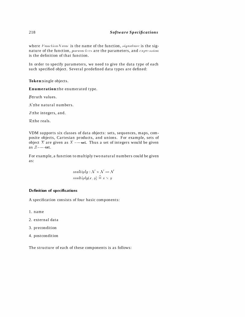
218 Software Specifications
where FunctionName is the name of the function, signature is the sig-nature of the function, parameters are the parameters, and expressionis the definition of that function.
In order to specify parameters, we need to give the data type of eachsuch specified object. Several predefined data types are defined:
Token:single objects.
Enumeration:the enumerated type.
B:truth values.
N :the natural numbers.
Z:the integers, and.
R:the reals.
VDM supports six classes of data objects: sets, sequences, maps, com-posite objects, Cartesian products, and unions. For example, sets ofobject X are given as X � �set. Thus a set of integers would be givenas Z� � set.
For example, a function to multiply two natural numbers could be givenas:
multiply : N �N � N
multiply�x� y��� x� y
De�nition of speci�cations
A specification consists of four basic components:
1. name
2. external data
3. precondition
4. postcondition
The structure of each of these components is as follows:
Specification Models 219
1. name: Name gives the name of the function to be defined and itssignature. It uses a notation similar to a Pascal function declaration.For example, to create a function multiply that takes two parametersx and y and produces an integer result z, the specification would be:
multiply : �x : Z; y : Z� : z : Z;
In this case, z � multiply�x� y�.
2. external data: The external data segment of a specification is op-tional. When present it specifies the name of the variables used by thespecification, but defined elsewhere. The syntax is:
ext names : mode type
where names is a list of identifiers used by the specification and modedetermines how each variable is used. A mode of wr means that thevariables are “read–write” and can be altered by the specification, whilea mode of rd means that the variables are “read-only” and cannot bealtered.
For example, if integers a and b are accessed by a specification and c isaltered, the external declaration could be given as:
ext a� b : rd Z;ext c : wr Z;
3. precondition: The precondition is specified as:
pre expression
where expression is any Boolean expression involving the variables ofthe specification.
For the multiply example given above, if we let pre � �multiply be apredicate describing the precondition, we can refer to this preconditionin formulae as pre�multiply�x� y�, which in this case would just be thepredicate true.
4. postcondition: The postcondition is specified as:
post expression
where expression is any boolean expression involving the variables ofthe specification. The postcondition generally specifies the functional-ity that is desired by the specification.
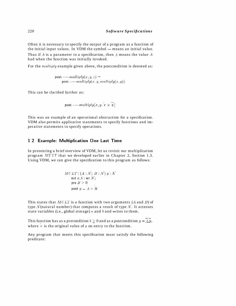
220 Software Specifications
Often it is necessary to specify the output of a program as a function ofthe initial input values. In VDM the symbol � means an initial value.Thus if A is a parameter to a specification, then
�
A means the value Ahad when the function was initially invoked.
For the multiply example given above, the postcondition is denoted as:
post ��multiply�x� y� z� �post ��multiply�x� y�multiply�x� y��
This can be clarified further as:
post� �multiply�x� y��x �
�y �
This was an example of an operational abstraction for a specification.VDM also permits applicative statements to specify functions and im-perative statements to specify operations.
���� Example� Multiplication One Last Time
In presenting a brief overview of VDM, let us revisit our multiplicationprogram MULT that we developed earlier in Chapter 2, Section 1.3.Using VDM, we can give the specification to this program as follows:
MULT : �A : N ; B : N � y : Next a� b : wr N ;pre B � 0post y �
�
A ��
B
This states that MULT is a function with two arguments (A and B) oftype N (natural number) that computes a result of type N . It accessesstate variables (i.e., global storage) a and b and writes to them.
This function has as a precondition b � 0 and as a postcondition y ��
A�
B,where
�x is the original value of x on entry to the function.
Any program that meets this specification must satisfy the followingpredicate:
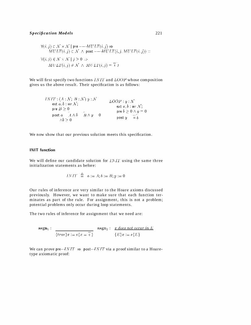
Specification Models 221
��i� j� � N � N j pre ��MULT �i� j� MULT �i� j� � N post ��MULT �i� j�MULT �i� j�� �
��i� j� � N � N j j � 0 MULT �i� j� � N MULT �i� j� �
����
We will first specify two functions INIT and LOOP whose compositiongives us the above result. Their specification is as follows:
INIT : �A : N ; B : N � y : Next a� b : wr N ;pre B � 0post a �
�
A b ��
B y � 0b � 0
LOOP : y : Next a� b : wr N ;pre b � 0 y � 0post y �
�a�
b
We now show that our previous solution meets this specification.
INIT function
We will define our candidate solution for INIT using the same threeinitialization statements as before:
INIT�� a :� A; b :� B; y :� 0
Our rules of inference are very similar to the Hoare axioms discussedpreviously. However, we want to make sure that each function ter-minates as part of the rule. For assignment, this is not a problem;potential problems only occur during loop statements.
The two rules of inference for assignment that we need are:
asgn1 : asgn2 : x does not occur in E
ftruegx :� efx ��e g fEgx :� efEg
We can prove pre�INIT post�INIT via a proof similar to a Hoare-type axiomatic proof:
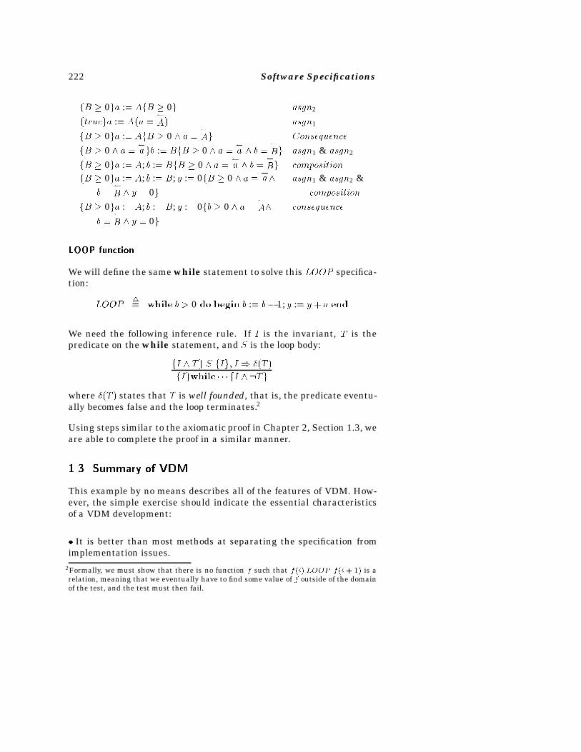
222 Software Specifications
fB � 0ga :� AfB � 0g asgn2
ftruega :� Afa ��Ag asgn1
fB � 0ga :� AfB � 0 a ��
Ag Consequence
fB � 0 a ��agb :� BfB � 0 a �
�a b �
�
Bg asgn1 & asgn2
fB � 0ga :� A; b :� BfB � 0 a ��a b �
�
Bg composition
fB � 0ga :� A; b :� B; y :� 0fB � 0 a ��a asgn1 & asgn2 &
b ��
B y � 0g composition
fB � 0ga :� A; b :� B; y :� 0fb � 0 a ��
A consequence
b ��
B y � 0g
LOOP function
We will define the same while statement to solve this LOOP specifica-tion:
LOOP�� while b � 0 do begin b :� b� 1; y :� y � a end
We need the following inference rule. If I is the invariant, T is thepredicate on the while statement, and S is the loop body:
fI Tg S fIg� I �T �
fIgwhile � � � fI �Tg
where �T � states that T is well founded, that is, the predicate eventu-ally becomes false and the loop terminates.2
Using steps similar to the axiomatic proof in Chapter 2, Section 1.3, weare able to complete the proof in a similar manner.
���� Summary of VDM
This example by no means describes all of the features of VDM. How-ever, the simple exercise should indicate the essential characteristicsof a VDM development:
� It is better than most methods at separating the specification fromimplementation issues.
2Formally, we must show that there is no function f such that f�i� LOOP f�i� 1� is arelation, meaning that we eventually have to find some value of f outside of the domainof the test, and the test must then fail.
Specification Models 223
� It can be completely formal, but can also be used informally.
� It can be used at several levels – proving a design meets a specifica-tion, or proving that a source program meets the specs.
� While practical, the process is still not easy.
�� TEMPORAL LOGIC
As we have discussed the issue of program correctness in this book,we have been concerned about the effects of certain programming lan-guage structures on the results of executing that program. Thus, wehave been mostly addressing the question “If I execute a program undercertain input constraints, will I get the desired result?” No mentionis ever made of when one can expect such results. Most correctnessmodels simply deal with the issue of whether the desired results even-tually will or will not occur. We have ignored the passage of time inthis discussion.
We can, however, include time within our logical system, and we callsuch models temporal logics. In this section, we briefly describe suchlogics and outline their major properties.
���� Properties of Temporal Logics
When we considered axiomatic correctness (via Hoare axioms of Chap-ter 2 or predicate transforms of Chapter 4) we were mostly concernedwith the question: “If predicate P is true and program S is executed,will predicate Q be true whenever S terminates?” When we considerthe question of when program S terminates, we can ask additional ques-tions. The following list is indicative of the kinds of issues temporallogic addresses:
� Safety property: Can something bad ever happen?
� Liveness property: Does something good eventually happen?
� Deadlock property: Does the program ever enter a state where nofurther progress is possible?
� Mutual exclusion: Can we ever have two different processes in thesame critical state at the same time?
224 Software Specifications
We can also represent our traditional programming logic as a temporalquestion: If the precondition is initially true, then is it possible for theprogram to terminate with the postcondition false?
For programs that execute sequentially, such as those usually writtenin Pascal, FORTRAN, or even C, the techniques given earlier in thisbook should suffice. However, when we consider simultaneous exe-cution of sets of these programs, such as the concurrent execution ofa set of processes within an operating system, the results are not soclear, and it is necessary to resort to techniques, like temporal logic, todetermine the correct behavior of the system.
Primitive temporal operators
Predicate calculus provides for the evaluation of expressions of Booleanvariables. In order to discuss time, we need to add two operators to ourpredicate calculus (of Chapter 2, Section 5):
� �: Now and forever
� �: Now or sometime in the future
Thus �p means that p is true now and remains true forever. Theexpression � p means that p is either true now or will eventuallybecome true.
The differences between these operations can be given by the followingexamples:
� x � 0 The expression is now true, and may be true orfalse in the future.
� ��x � 0� The expression is now true and will remain trueforever.
� � �x � 0� The expression will sometime be true (eithernow or later).
We will call our expressions of temporal logic assertions. Any assertionwhich does not contain any of the temporal operators will be called apredicate and is obviously equivalent to the predicate calculus predi-cates we studied before.
Specification Models 225
Non�primitive operators
For convenience, we will introduce the following two nonprimitive op-erators: � and �.
This � is defined as the dual to �. That is:
�p�� ���p
Since ��p states that it is always true that p is never true (i.e., thatp is always false), �p states that it is not never true that p is alwaysfalse. So does this mean that �p is sometimes true and �p �� p? Theanswer is an unqualified “maybe.”
To understand this statement, consider that developing temporal as-sertions is further complicated by the realization that we have at leasttwo definitions of time. In one case, we view time as a linear sequenceof events, while in the other we view time as all possible events thatmay occur in the future, much like the distinction between nonde-terministic and deterministic state machines when discussing formalcomputational models. We call the former linear-time and the latterbranching-time temporal logic.
With linear-time logic, there is a single time line of future events de-termining what will happen. There is only one possible future, so “notnever” does indeed mean sometime, and we do have the equivalence:�p �� p.
However, with branching time logic, at each instance there may bealternative applicable choices, thus forming a tree of future actions. pmay become true on some path that depends upon a future decision.Since p may become true since that path may be traversed, we can saythat �p is true. However, we cannot say that � p is true since we donot yet know if that path that makes p true must be traversed.
Obviously, a single future to deal with is simpler than branching-timelogic, and we will restrict the discussion in this chapter to linear timelogic where �p �� p.
A second nonprimitive operator is leadsto, the “leads to” operator, whichis defined to be:
P � Q�� ��P �Q�
226 Software Specifications
That is, P � Q means that it is always true that if P is ever true, theneventually (i.e., sometimes) Q will be true. We will see this operatoragain when we discuss verification conditions for concurrent programs.
States
Much like other programming language models described earlier, wecan describe temporal assertions by their effects upon system states.However, since we need to consider concurrent execution where severalprogram statements may execute next, we need to include a “next state”component to our model. In the sequential model, we could have simplymodeled the next state function as a mapping from location counter tostatement number. However, here there may be more than one nextstate ready for execution.
We define a state s as the pair: (1) a function from names to values,and (2) a set ready giving the set of statements available for execution.We let S be the set of all such states.
In discussing the issues of safety, liveness, and other such properties,we are usually concerned about the sequence of states that a programpasses through. We write such a sequence as s � s0� s1� s2� � � � whereeach si is in S.
If s is a sequence of states, the tail of that sequence (i.e., the sequencewith the first element deleted) is given by s�, that is: �s��i � si�1.
We define the semantics of a program as all valid execution sequencesthat a program may have. For traditional programming languages,there will be a single execution sequence describing the behavior of aprogram; however, as we add parallel processing and distributed com-puting primitives, a program may have more than one valid executionsequence. (We saw some of this with the guarded commands of Dijkstraearlier.)
Immediate assertions
We combine our notion of predicates with concurrent states via imme-diate assertions and the operator j�. We write s j� P to state that Phas value true in state s. That is, if s �� f� ready �, then values of fapplied to P result in P being true.
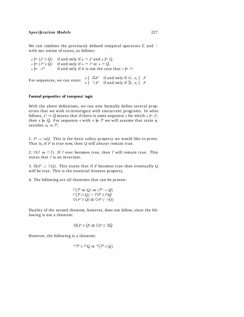
Specification Models 227
We can combine the previously defined temporal operators � and �with our notion of states, as follows:
s j� �P Q� if and only if s j� P and s j� Q.s j� �P �Q� if and only if s j� P or s j� Q.s j� �P if and only if it is not the case that s j� P .
For sequences, we can state: s j� �P if and only if �i� si j� Ps j� �P if and only if �i� si j� P
Formal properties of temporal logic
With the above definitions, we can now formally define several prop-erties that we wish to investigate with concurrent programs. In whatfollows, P Q means that if there is some sequence s for which s j� P ,then s j� Q. For sequence s with s j� P we will assume that state s0satisfies s0 j� P :
1. P �Q. This is the basic safety property we would like to prove.That is, if P is true now, then Q will always remain true.
2. ��I �I�. If I ever becomes true, then I will remain true. Thisstates that I is an invariant.
3. ��P �Q�. This states that if P becomes true then eventually Qwill be true. This is the essential liveness property.
4. The following are all theorems that can be proven:
��P Q� �P � Q���P Q� � �P �Q��P �Q� � �P ��Q�
Duality of the second theorem, however, does not follow, since the fol-lowing is not a theorem:
��P �Q� � �P ��Q
However, the following is a theorem:
�P ��Q ��P �Q�
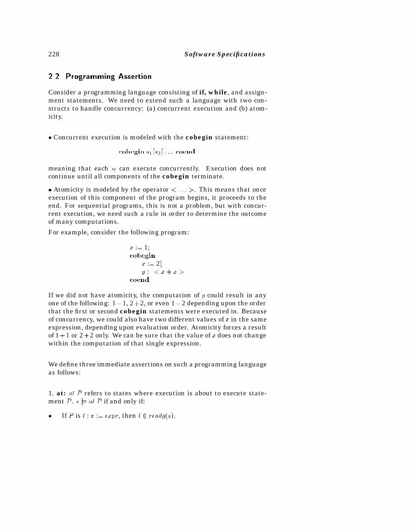
228 Software Specifications
���� Programming Assertion
Consider a programming language consisting of if, while, and assign-ment statements. We need to extend such a language with two con-structs to handle concurrency: (a) concurrent execution and (b) atom-icity.
� Concurrent execution is modeled with the cobegin statement:
cobegin s1��s2�� � � � coend
meaning that each si can execute concurrently. Execution does notcontinue until all components of the cobegin terminate.
� Atomicity is modeled by the operator � � � � �. This means that onceexecution of this component of the program begins, it proceeds to theend. For sequential programs, this is not a problem, but with concur-rent execution, we need such a rule in order to determine the outcomeof many computations.
For example, consider the following program:
x :� 1;cobegin
x :� 2��y :�� x� x �
coend
If we did not have atomicity, the computation of y could result in anyone of the following: 1�1, 2�2, or even 1�2 depending upon the orderthat the first or second cobegin statements were executed in. Becauseof concurrency, we could also have two different values of x in the sameexpression, depending upon evaluation order. Atomicity forces a resultof 1�1 or 2�2 only. We can be sure that the value of x does not changewithin the computation of that single expression.
We define three immediate assertions on such a programming languageas follows:
1. at: at P refers to states where execution is about to execute state-ment P . s j� at P if and only if:
� If P is l : x :� expr, then l � ready�s�.
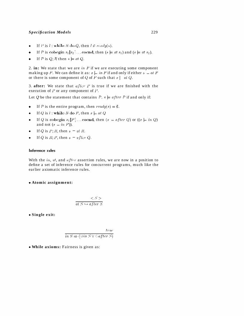
Specification Models 229
� If P is l : while B do Q, then l � ready�s�.
� If P is cobegin s1��s2�� � � �coend, then (s j� at s1) and (s j� at s2).
� If P is Q;R then s j� at Q.
2. in: We state that we are in P if we are executing some componentmaking up P . We can define it as: s j� in P if and only if either s j� at Por there is some component of Q of P such that s j� at Q.
3. after: We state that after P is true if we are finished with theexecution of P or any component of P .
Let Q be the statement that contains P . s j� after P if and only if:
� If P is the entire program, then ready�s� � �.
� If Q is l : while B do P , then s j� at Q
� If Q is cobegin s1��P �� � � �coend, then �s j� after Q� or ((s j� in Q)and not (s j� in P )).
� If Q is P ;R, then s j� at R.
� If Q is R;P , then s j� after Q.
Inference rules
With the in, at, and after assertion rules, we are now in a position todefine a set of inference rules for concurrent programs, much like theearlier axiomatic inference rules.
� Atomic assignment:
� S �
at S � after S
� Single exit:
true
in S ��in S ��after S�
� While axioms: Fairness is given as:
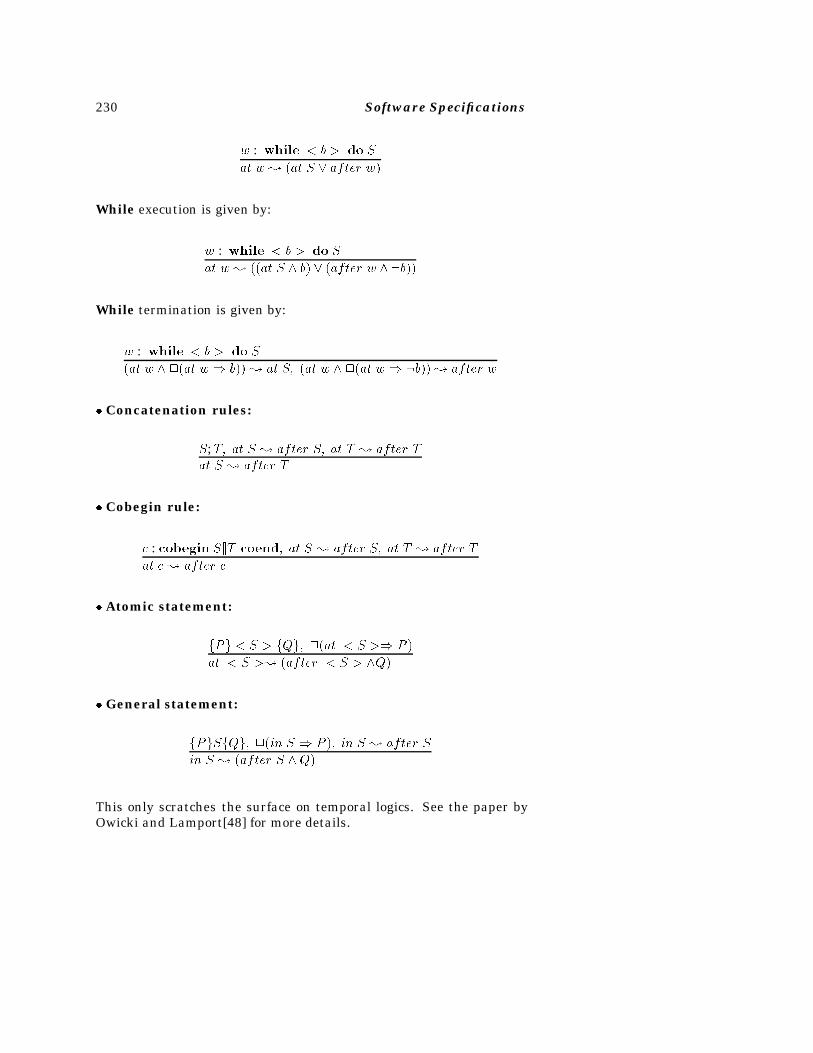
230 Software Specifications
w : while � b � do S
at w� �at S � after w�
While execution is given by:
w : while � b � do S
at w� ��at S b� � �after w �b��
While termination is given by:
w : while � b � do S
�at w ��at w b��� at S� �at w ��at w �b��� after w
� Concatenation rules:
S;T� at S � after S� at T � after Tat S � after T
� Cobegin rule:
c : cobegin S��T coend� at S � after S� at T � after T
at c� after c
� Atomic statement:
fPg � S � fQg� ��at � S � P �
at � S �� �after � S � Q�
� General statement:
fPgSfQg� ��in S P �� in S � after S
in S � �after S Q�
This only scratches the surface on temporal logics. See the paper byOwicki and Lamport[48] for more details.
Specification Models 231
�� RISK ANALYSIS
While there are many other attributes which can affect a specification,their enumeration is beyond the scope of this book. Suffice it to saythat resource estimation and safety analysis are representative of theothers.
Assume we have a set of such attributes which define a specificationto a program. How does one choose an appropriate design that meetsthat specification? We know that a complete specification needs toaddress many attributes, including functionality, resource usage, se-curity, safety, and other concerns. Most designs will meet certain re-quirements well and probably not meet others.
How do we know what project to build? How do we assess the riskfor each decision? Will prototyping reduce this risk? All of these areimportant considerations, and have only recently been applied to thespecification problem.
We now describe one such evaluation strategy. It consists of two compo-nents. In one, the designer knows all relevant details (decision undercertainty). In the second case, there is some variability (and risk)associated with all potential choices. We call this decision under un-certainty.
���� Decisions under Certainty
We consider correct functionality to be just one of several attributes fora solution, with multiple designs implementing the same functionality.Let us first assume that our needed functionality is specified by a func-tion (from state to state) and also the candidate programs are specifiedby functions from state to state. Let X be the functionality of programx. We extend this model to include other attributes as well. Since theseother attributes are often concerned with nonfunctional characteristicssuch as resource usage, schedules, and performance, we will use theterm viable for any solution satisfying a specification rather that themore specific term correctness.
Now assume that our specifications (for both our needed software andthe candidate programs) are vectors of attributes, including the func-tionality as one of the elements of the vectors. For example, X and Yare vectors of attributes that specify alternative solutions to a specifi-
232 Software Specifications
cation B. Let S be a vector of objective functions with domain beingthe set of specification attributes and range �0��1�. We call Si a scalingfunction and it is the degree to which a given attribute meets its goal.We state that X solvesS Y if �i� Si�Xi� � Si�Yi�. We extend our previ-ous definition of correctness to the following: design x is viable (i.e., iscorrect) with respect to specification B and scaling function vector S ifand only if P solvesS B. We can show that the previous definition ofcorrectness is simply a one-dimensional example of this more generaldefinition of viability.
Each attribute may not have the same importance. Assume a vector ofweights W called constraints such that each wi � �0��1� and
Pwi � 1�
Our evaluation measure, the performance level, merges multiple scaledattributes and their constraints. Given specification vector X, scal-ing function S and constraints W , the performance level is given by:PL�X�S�W � �
Pi�wi � Si�Xi��.
We use the performance level as our objective function: Given a specifi-cation vector B, scaling vector S, constraints W , and potential solutionsx and y, X improves Y with respect to hB� S�W i if and only if:
1. X solvesS B and Y solvesS B
2. PL�X�S�W � � PL�Y� S�W �.
We use here a very simple weighted sum to compute the performancelevel. Our definition of improves depends only upon an appropriatedefinition of performance level for comparing two solutions, not on thedetails of how the two vectors are compared.
It should be noted that the model presented in this section dependsupon the solution triple hB� S�W i, which is a quantitative evaluationof how well each attribute of the proposed solution meets or exceedsthe minimal specification B. We rarely know this in practice and thisbook only assumes an ordinal ranking of the attributes – that is, oneattribute value is better than another.
���� Decisions under Uncertainty
We have so far assumed that the relative importance of each attributeis known a priori. However, we rarely know this with certainty. We
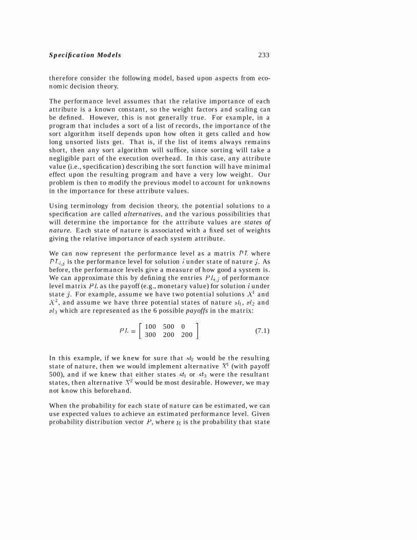
Specification Models 233
therefore consider the following model, based upon aspects from eco-nomic decision theory.
The performance level assumes that the relative importance of eachattribute is a known constant, so the weight factors and scaling canbe defined. However, this is not generally true. For example, in aprogram that includes a sort of a list of records, the importance of thesort algorithm itself depends upon how often it gets called and howlong unsorted lists get. That is, if the list of items always remainsshort, then any sort algorithm will suffice, since sorting will take anegligible part of the execution overhead. In this case, any attributevalue (i.e., specification) describing the sort function will have minimaleffect upon the resulting program and have a very low weight. Ourproblem is then to modify the previous model to account for unknownsin the importance for these attribute values.
Using terminology from decision theory, the potential solutions to aspecification are called alternatives, and the various possibilities thatwill determine the importance for the attribute values are states ofnature. Each state of nature is associated with a fixed set of weightsgiving the relative importance of each system attribute.
We can now represent the performance level as a matrix PL wherePLi�j is the performance level for solution i under state of nature j. Asbefore, the performance levels give a measure of how good a system is.We can approximate this by defining the entries PLi�j of performancelevel matrix PL as the payoff (e.g., monetary value) for solution i understate j. For example, assume we have two potential solutions X1 andX2, and assume we have three potential states of nature st1, st2 andst3 which are represented as the 6 possible payoffs in the matrix:
PL �
�100 500 0300 200 200
�(7.1)
In this example, if we knew for sure that st2 would be the resultingstate of nature, then we would implement alternative X1 (with payoff500), and if we knew that either states st1 or st3 were the resultantstates, then alternative X2 would be most desirable. However, we maynot know this beforehand.
When the probability for each state of nature can be estimated, we canuse expected values to achieve an estimated performance level. Givenprobability distribution vector P , where pi is the probability that state
234 Software Specifications
of nature sti is true, the expected payoff for alternative Xi is given by:
vi �Xj
pli�j pj
Use the decision rule: Choose Xi which maximizes vi or:
maxi
�Xj
pli�j pj�
For example, if we know that the probability distribution for each stateof nature in our example is: P = (0.3, 0.5, 0.2), we can calculate theexpected payoffs as follows:
v1 � 100 � 0�3 � 500 � 0�5 � 0� 0�2� 280
v2 � 300 � 0�3 � 200 � 0�5 � 200� 0�2� 230
We would then choose X1 over X2 since 280 � 230.
���� Risk Aversion
Risk aversion plays an important role in decision making. This impliessubjective behavior on the part of the software manager. We assumethat the following reasonable behavior rule (i.e., equilibrium probabil-ity) is true:
� Decomposition: Given three payoffs a � b � c, there exists a prob-ability � such that the decision maker is indifferent to the choice ofa guarantee of b, and the choice of getting c with probability � andgetting a with probability 1 � �. We shall refer to this probability asdecomp�a� b� c�.
For example, assume there are two techniques to solve a problem. Oneis fully tested, giving a guaranteed payoff of $5,000 and a second newand more efficient technique promises a potentially larger payoff of$10,000 (but not completely tested) with a chance to give a payoff ofonly $2,000. If a software manager considers using the new techniqueonly if the chances of getting the payoff of $10,000 are larger than 80%,the probability � is larger than 0.8. In this case, the expected payoffwill be 10,000 � 0.8 + 2,000 � 0.2 = 8,400, so the given manager issomewhat risk-averse and conservative.
Specification Models 235
Let pl0 be the minimal value in our payoffPL and let pl� be the maximalvalue. In our example PL matrix (Section 3.1), we would choose pl� �500 and pl0 � 0. We decompose each pli�j as ei�j � decomp�pl0� pli�j� pl
�� �.This decomposition creates an equivalent pair of payoffs fpl0, pl�g, withprobability ei�j of getting the more desirable pl�. We call the matrixformed by these elements ei�j ’s the equilibrium matrix E.
Any element ei�j will satisfy the following inequality:
pl0 � �1� ei�j� � pl� � ei�j � pli�j
The difference between the two sides of this equation reflects the man-ager’s degree of risk averseness. If the two sides are equal, risk analysisreduces to the expected value.
���� Value of Prototyping
Given the various unknowns in the states of nature, the software man-ager may choose to get more information with a prototype so that abetter final decision can be made. However, before undertaking theprocedure to extract more information, one should be sure that the gaindue to the information will outweigh the cost of obtaining it. Here, wetry to establish an absolute boundary: What is the value of perfectinformation?
The best we can expect is that the results of the experiment will indicatefor sure which state of nature will hold. Under this case, we can choosethe alternative that gives the highest performance level under the givenstate of nature:
�Xj
pj �maxi
pli�j
In our example, we would chooseX1 under st2 and chooseX2 otherwise,resulting in performance level :
� 0�3� 300 � 0�5� 500 � 0�2� 200� 380
What is the value of this perfect information? Since the expected valueof our performance level was computed previously as 280, the value ofthis information is an improvement in performance level of 380�280 �100. This is the most that we can expect our prototype to achieve andstill be cost effective.
236 Software Specifications
Assume we build a prototype to test which state of nature will betrue. While we would like an exact answer, since a prototype is onlyan approximation to the real system, the results from prototyping areprobabilistic. Let result1, result2, ... resultk be the possible resultsof the prototype. This information will be presented in a conditionalprobability matrix C where ci�j represents the conditional probabilityof result resulti given state of nature Sj .
Given the probabilities for each state (vector P) and the conditionalprobability matrix C, the marginal probability distribution (vector Q)for obtaining resulti is given by:
qi �Xj
ci�j � pj
We can compute the a posteriori distribution matrix P�. P � has as manyrows as results from the prototype which are updated values of vectorP . Row i gives the probabilities of the states of nature given that theresult of the prototype is resulti:
p�i�j �ci�j � pj
qi
Following our example, assume that a prototype of alternative X2 isplanned. The planned prototype can give the following results:
1. result1: We are satisfied with the system as presented by prototype.
2. result2: We are not satisfied.
Assume that the conditional probabilities are estimated beforehand.For example, we estimate that if the state of nature is st2, we haveprobabilities 0.3 and 0.7 to obtain results result1 and result2 respec-tively from the prototype. The conditional probabilities appear in thematrix C having a column for each state and a row for each result ofthe prototype:
C �
�0�9 0�3 0�40�1 0�7 0�6
�
From this we can calculate the probability qi for each result i of the pro-totype, giving Q � �0�5� 0�5�, and the a posteriori distribution matrix:
P � �
�0�54 0�30 0�160�06 0�70 0�24
�
Specification Models 237
If, for example, we get result1 from the prototyping study, the newexpected values for alternatives X1 and X2 are:
v1 � 100� 0�54 � 500 � 0�3 � 0� 0�16� 204
v2 � 300� 0�54 � 200 � 0�3 � 200� 0�16� 254
In this case, alternative X2 should be chosen, since it gives the higherperformance level.
Similarly, if we should get result2 from the prototyping study, the newperformance levels for alternatives X1 and X2 are:
v1 � 100� 0�06 � 500 � 0�7 � 0� 0�16� 356
v2 � 300� 0�06 � 200 � 0�7 � 200� 0�24� 206
In this case, alternative X1 is the preferred choice.
Given that our expected performance level with no information was280 (Section 3.2), we should only prototype if we gain from prototyping:
vP � 0�5� 356 � 0�5� 254� 280� 25
Since there is a positive gain vP � 25, prototyping should be carriedout as long as the cost to construct the prototyping study is less thanthis. Otherwise, an immediate decision should be made.
�� SUGGESTED READINGS
The Woodcock and Loomes paper describes a notation similar to Z.
� J. Woodcock and M. Loomes, Software Engineering Mathematics,Addison-Wesley, Reading, MA, 1988.
� C. B. Jones, Systematic Software Development using VDM, Prentice-Hall, Englewood Cliffs, NJ, 1990.
238 Software Specifications
� M. I. Jackson, “Developing Ada programs using the Vienna Develop-ment Method (VDM),” Software Practice and Experience, Vol. 15, No.3, 1985, pp. 305-318.
� A. Hall, “Seven myths of formal methods,” IEEE Software, Vol. 7, No.5, 1990, pp. 11-19.
� J. Wing, “A specifier’s introduction to formal methods,” IEEE Com-puter, vol. 23, No. 9, 1990, pp. 8-24.
Temporal logic is covered in greater detail in:
� L. Lamport, “‘Sometime’ is sometimes ‘not never,:’ On the temporallogic of programs,” Proceedings of the 7th ACM Principles of Program-ming Language Conference, Las Vegas, NV, 1980, pp. 174-185.
� S. Owicki and L. Lamport, “Proving liveness properties of concur-rent programs,” ACM Transactions on Programming Languages andSystems Vol. 4, No. 3, 1982, pp. 455-495.
The section on risk analysis is described in:
� S. Cardenas and M. V. Zelkowitz, “Evaluation criteria for functionalspecifications,” Proceedings of the ACM/IEEE 12th International Con-ference on Software Engineering, Nice, France, March 1990, pp. 26-33.
� S. Cardenas, and M. V. Zelkowitz, “A management tool for evaluationof software designs,” IEEE Transactions on Software Engineering, Vol.17, No. 9, , 1991.

Bibliography
[1]A. Aho, R. Sethi, and J. Ullman, Compilers: Principles, Techniquesand Tools, Addison-Wesley, Reading, MA, 1986.
[2]S. K. Basu and R. T. Yeh, “Strong Verification of Programs,” IEEETransactions on Software Engineering, Vol. 1, No. 3, 1975, pp. 339-346.
[3]J. Bentley, Programming Pearls, Addison-Wesley, Reading, MA,1986.
[4]R. S. Boyer and J. S. Moore, “Proving Theorems about LISP Func-tions,” Journal of the ACM, Vol. 22, 1975, pp. 129-144.
[5]R. Burstall, “Proving Properties of Program by Structural Induc-tion,” Computer Journal, Vol. 12, 1969, pp. 41-48.
[6]S. Cardenas and M. V. Zelkowitz, “Evaluation criteria for functionalspecifications,” Proceedings of the ACM/IEEE 12th InternationalConference on Software Engeering, Nice, France, 1990, pp. 26-33.
[7]S. Cardenas and M. V. Zelkowitz, “A management tool for evalu-ation of software designs,” IEEE Transactions on Software Engi-neering, Vol. 17, No. 9, 1991.
[8]S. A. Cook, “Soundness and Completeness of an Axiom System forProgram Verification,” SIAM Journal of Computing, Vol. 7, 1978,pp. 70-90.
[9]D. Craigen (Ed.), Formal methods for trustworthy computer systems(FM89), Springer Verlag, New York, 1990.
[10]E. W. Dijkstra, “Guarded commands, nondeterminacy and formalderivation of programs,” Communications of the ACM, Vol. 18, No.8, 1975, pp. 453-458.
239
240 Software Specifications
[11]E. W. Dijkstra, A Discipline of Programming, Prentice-Hall, Engle-wood Cliffs, NJ, 1976.
[12]D. D. Dunlop and V.R. Basili, “A Comparative Analysis of Func-tional Correctness,” ACM Computing Surveys, Vol. 14, No. 2, 1982,pp. 229-244.
[13]D. D. Dunlop and V.R. Basili, “A Heuristic for Deriving Loop Func-tions,” IEEE Transactions on Software Engineering, Vol. 10, 1984,pp. 275-285.
[14]C. N. Fischer and R. J. LeBlanc, Crafting a compiler, BenjaminCummings, Menlo Park, CA, 1988.
[15]L. Flon and J. Misra, “A Unified Approach to the Specificationand Verification of Abstract Data Types,” Proceedings of the IEEEConference on Specifications of Reliable Software, Cambridge, MA,,1979, pp. 162-169.
[16]R. W. Floyd, “Assigning Meanings to Programs,” Symposium inApplied Mathematics, 19, 1967, pp. 19-32.
[17]R. Forgaard and J. V. Guttag, “REVE: A term rewriting systemgenerator with failure resistant Knuth-Bendix,” Workshop on theRewrite Rule Laboratory, National Science Foundation, 1984, pp.5-31.
[18]J. D. Gannon, R. B. Hamlet, and H. D. Mills, “Theory of Modules,”Transactions on Software Engineering, Vol. 13, No. 7, 1987, pp.820-829.
[19]S. Gerhart, “An Overview on AFFIRM: a Specification and Verifi-cation System,” in Information Processing, Vol. 80 (S.H. Lavington(Ed)), North Holland, 1980, pp. 343-387.
[20]J. A. Goguen, J.W. Thatcher, and E.G. Wagner, “An Initial AlgebraApproach to the Specification, Correctness, and Implementation ofAbstract Data Types,” in Current Trends in Programming Method-ology, Vol. 4, (R. T. Yeh (Ed)), Prentice-Hall, Englewood Cliff, NJ,1978, pp. 80-149.
[21]J. A. Goguen, “How to Prove Algebraic Inductive Hypotheses with-out Induction,” LNSC, Vol. 87, Springer-Verlag, New York, 1980,pp 356-373.
[22]D. Gries and G. Levin, “Assignment and Procedure Call ProofRules,” Transactions on Programming Languages and Systems, Vol.2, No. 4, 1980, pp. 564-579.
Bibliography 241
[23]D. Gries, The Science of Programming, Springer-Verlag, New York,1981.
[24]J. V. Guttag and J.J. Horning, “The Algebraic Specification of Ab-stract Data Types,” Acta Informatica, Vol. 10, 1978, pp. 27-52.
[25]J. V. Guttag, E. Horowitz, and D. Musser, “Abstract Data Types andSoftware Validation,” Communications of the ACM, Vol. 21, 1978,pp. 1048-1064.
[26]J. V. Guttag, E. Horowitz, and D. R. Musser, “The Design of DataType Specifications,” in Current Trends in Programming Methodol-ogy 4: Data Structuring, (R. T. Yeh (Ed)) Prentice-Hall, EnglerwoodCliffs, NJ, 1978, pp. 60-79.
[27]J. V. Guttag, “Notes on Type Abstraction (Version 2),” IEEE Trans-actions on Software Engineering, Vol. 6, No. 1, 1980, pp. 13-23.
[28]A. Hall. “Seven myths of formal methods,” IEEE Software Vol. 7,No. 5, 1990, pp. 11-19.
[29]C. A. R. Hoare, “An Axiomatic Basic for Computer Programming,”Communications of the ACM, Vol. 12, No. 10, 1969, pp. 576-580,583.
[30]C. A. R. Hoare, “Procedures and Parameters, An Axiomatic Ap-proach,” Symposium on the Semantics of Algorithmic Languages,Springer-Verlag, New York, 1971, pp. 102-116.
[31]C. A. R. Hoare, and N. Wirth, “An Axiomatic Definition of theProgramming Language PASCAL,” Acta Informatica, Vol. 2, 1973,pp. 335-355.
[32]G. Huet, “Confluent Reductions: Abstract Properties and Appli-cations to Term-Rewriting Systems,” Journal of the ACM, Vol. 27,1980, pp. 797-821.
[33]G. Huet and J.-M. Hullot, “Proofs by Induction in Equational Theo-ries with Constructors,” Journal of Computer and System Science,Vol. 25, 1982, pp. 239-266.
[34]J-M. Hullot, “Canonical Forms and Unification,” LNSC, Vol. 87,Springer-Verlag, New York, 1980, pp. 318-334.
[35]C. B. Jones, Systematic Software Development using VDM,Prentice-Hall, Englewood Cliffs, NJ, 1990.
242 Software Specifications
[36]M. I. Jackson, “Developing Ada programs using the Vienna Devel-opment Method (VDM),” Software Practice and Experience, vo. 15,No. 3, 1985, pp. 305-318.
[37]S. Kamin, “The Expressive Theory of Stacks,” Acta Informatica,Vol. 24, 1987, pp. 695-709.
[38]D. E. Knuth and P.B. Bendix, “Simple Word Problems in Univer-sal Algebras,” in Computational Problems in Abstract Algebras, J.Leech (ed)), Pergamon Press, New York, 1970, pp. 263-297.
[39]L. Lamport, “‘Sometime’ is sometimes ‘not never,:’ On the temporallogic of programs,” Proceedings of the 7th ACM Prin. of Program-ming Languages Conference, Las Vegas, NV, 1980, pp. 174-185.
[40]L. Lamport and F. B. Schneider, “The ‘Hoare Logic’ of CSP, and AllThat,” Transactions on Programming Languages and Systems, Vol.6, No. 2, 1984, pp. 281-296.
[41]R. C. Linger, H. D. Mills, and B. I. Witt, Structured Programming:Theory and Practice, Addison-Wesley, Reading, MA, 1979.
[42]B. Liskov and J. Guttag, Abstraction and Specification in ProgramDevelopment, MIT Press, McGraw-Hill, New York, NY, 1986.
[43]D. C. Luckham and N. Suzuki. “Verification of Array, Record, andPointer Operations in Pascal,” Trans on Programming Languagesand Systems, Vol. 1, No. 2, 1979, pp. 226-244.
[44]H. D. Mills, “The New Math of Computer Programming,” Commu-nications of the ACM, Vol. 18, No. 1, 1975, pp. 43-48.
[45]H. D. Mills, V. R. Basili, J. D. Gannon and R. G. Hamlet. Principlesof Computer Programming: A Mathematical Approach, William C.Brown, Dubuque, IA, 1987.
[46]D. R. Musser, “Abstract data type specifications in the AFFIRMsystem,” IEEE Specifications of Reliable Software Conference, Cam-bridge MA, 1979, pp. 47-57.
[47]D. R. Musser, “On Proving Inductive Properties of Abstract DataTypes,” Proceedings of the 7th ACM Symposium on Principles ofProgramming Languages, 1980, pp. 154-162.
[48]S. Owicki and L. Lamport, “Proving liveness properties of concur-rent programs,” ACM Transactions on Programming Languagesand Systems, Vol. 4, No. 3, 1982, pp. 455-495.
Bibliography 243
[49]G. L. Peterson and M.E. Stickel, “Complete Sets of Reductions forSome Equational Theories,” Journal of the ACM, Vol. 28, 1981, pp.233-264.
[50]N. C. K. Phillips, “Safe Data Type Specification,” IEEE Software,Vol. 10, 1984, pp. 285-289.
[51]T. W. Pratt, Programming Languages: Design and Implementation,Prentice-Hall, Englewood Cliffs, NJ, 1984.
[52]J. H. Remmers, “A Technique for Developing Loop Invariants,” In-formation Processing Letters, Vol. 18, 1984, pp. 137-139.
[53]J. C. Reynolds, The Craft of Computer Programming, Prentice Hall,Englewood Cliffs, NJ, 1981.
[54]R. Sethi, Programming Languages: Concepts and Constructs,Addison-Wesley, reading, MA, 1989.
[55]J. Spitzen and B. Wegbreit, “The Verification and Synthesis of DataStructures,” Acta Informatica, Vol. 4, 1975, pp. 127-144.
[56]D. A. Schmidt, Denotational Semantics, Allyn and Bacon. NewYork, 1986.
[57]R. D. Tennent, “The denotational semantics of programming lan-guages,” Communications of the ACM, Vol. 19, No. 8, 1976, pp.437-453.
[58]P. Wegner, Programming Languages, Information Structures andMachine organization, McGraw Hill, New York, 1968, pp. 180-196.
[59]J. Wing, “A specifier’s introduction to formal methods,” IEEE Com-puter, Vol. 23, No. 9, 1990.
[60]J. Woodcock and M. Loomes, Software Engineering Mathematics,Addison-Wesley, Reading, MA, 1988.
[61]W. Wulf, M. Shaw, L. Flon, and P. Hilfinger, Fundamental structuresof Computer Science, Addison-Wesley, Reading, MA, 1980.
[62]W. Wulf, R. L. London and M. Shaw. “An introduction to the con-struction and verification of Alphard programs,” IEEE Transactionson Software Engineering, Vol. 2, No. 4, 1976, pp. 253-265.
[63]M. V. Zelkowitz, “A functional correctness model of program verifi-cation,” IEEE Computer, Vol. 23, No. 11, 1990, pp. 30-39.
244 Software Specifications
[64]M. V.Zelkowitz, “The role of verification in the software specifica-tion process,” in Advances in Computer, Vol. 36 (M. Yovits (ed)),Academic Press, Orlando, FL, 1993.

Author Index
Aho A., 28
Backus J., 5Basili V., 117Basu S. K., 134Bendix P., 169Bentley J., 28Bjorner D., 214
Cardenas S., 236Church A., 191Craigen D., 29
Dijkstra E. W., 6, 9, 10, 119, 134Dunlop D., 117
Fischer C., 28Flon L., 189Floyd R., 7, 9, 84
Gannon J. D., 117Gries D., 10, 28, 84, 134Guttag J., 10, 189
Hall A., 16, 29, 235Hamlet R., 117Hoare C. A. R., 9, 33, 37, 84Hopper G., 5Horning J., 152, 189Horowitz E., 189Huet G., 171, 190Hullot J., 190
Jackson M., 235Jones C., 214, 235
Knuth D., 169
Lamport L., 84, 228, 235LeBlanc R., 28Levin G., 84Linger R., 117Loomis M., 29, 235Luckham D., 84
McCarthy J., 90Mills H. D., 13, 14, 117Misra J., 189Musser D., 174, 189
Naur P., 5
Oppen D., 171Owicki S., 228, 235
Pratt T., 29
Remmers J., 84Reynolds J., 84
Schmidt D., 211Schneider F., 84Scott D., 14Sethi R., 28, 29Strachey C., 14Straub P., 145Suzuki N., 84
Tennent R., 211
Ullman J., 28
245
246 Software Specifications
Wegner P., 211Wing J., 29, 235Wirth N., 84Witt B. I., 117Woodcock J., 29, 235
Yeh R., 134, 189
Zelkowitz M. V., 1, 117, 236
Index
AdaData storage, 11Package, 108
Adaptation, 62, 71Existential quantifiers, 64Quantification, 63
ADT (Abstract data type), seeAlgebraic specifications
Algebraic specifications, 10, 135,139
Axioms, 140Consistency, 149Constructors, 139, 145Data type, 136Data type induction, 150Developing axioms, 142Equality, 150Hints for writing axioms, 145Rewrite rules, 141Signatures, 145Verification, 158Verifying implementations,
154Applicative languages
Data storage, 12Array assignment, 48Atomicity, 226Attribute grammars, 7Axiomatic verification, 7, 9
Adaptation, 62, 71Array assignment, 48Axioms, 31Composition axiom, 31Conditional, 33
Consequence axiom, 31If, 33Invariant, 34Postcondition, 8Precondition, 8Procedure call substitution,
59Procedure calls, 57Procedure invocation, 58Recursion, 72Termination, 38, 41While, 33
Bottom, 196Box notation, 13, 85Bug, see Software error
CClass, 108Data storage, 11
Completeness, 20Composition axiom, 31Concurrent assignment, 90Concurrent execution, 225Conditional axiom, 33Conditional functions, 22Conditional probability, 233Consequence axiom, 31Continuations, 208Continuity, 198Continuous functions, 197Correctness, 2
Weakest precondition, 122Critical pairs, 173
247
248 Software Specifications
Data abstraction, 107Data abstractions, 135
Encapsulation, 135Data storage models, 11Data type induction, 150
Inductionless induction, 169Datatypes, 195
Axioms, 195Deadlock, 221Decidable, 19Decisions
Certainty, 229Uncertainty, 230
Denotational semantics, 14, 191Aliasing, 207Assignment statement, 206,
208Begin statement, 206, 207Bottom, 196Composition, 206, 207Continuity, 198Continuous functions, 197Datatypes, 195Denotable values, 203Environment, 207Expressions, 204Factorial function, 199Fixed point, 200If statement, 206, 208Injection, 206Inspection, 205Pointers, 207Program semantics, 201Program statement, 203Projection, 206Recursive functions, 199Serious computation, 209State, 14Top, 196While statement, 206, 208
Domains, 196Simple, 197
Encapsulation, 135Equilibrium probability, 232Example
Array reversal, 166Data type induction, 153,
178Fast multiplication, 42Finite integers, 147Functional design, 103Functional verification, 98Inference system, 26Integer division, 34, 128Knuth–Bendix, 177Multiplication, 38, 104, 129,
218Reversing an array, 53Shifting an array, 50Simple recusion, 73Simple sums, 66Stack verification, 160
Fixed point, 200Formal methods
Limitations, 16FORTRAN
Data storage, 11Functional correctness, 13, 15,
85Assignment statement, 90,
93Begin statement, 93Box notation, 13, 85Concurrent assignment, 90Conditional statement, 91Correctness theorem, 85Design rules, 90If statement, 94Semantics, 86State, 86Statement execution, 87Statements, 87Symbolic execution, 88Termination, 97
Index 249
Trace table, 89Verification conditions, 92While loop design, 96While statement, 94
Guarded commands, 10, 119If statement, 120Repetitive statement, 120
Hoare axioms, see Axiomatic ver-ification
If axiom, 33Imperative languages
Data storage, 11Inductionless induction, 169Inference rules, 19
Modus ponens, 21Substitution, 21
Initial value (�), 22Injection, 206Inspection, 205Invariant, 34
Chossing, 47Iteration theorem, 125
Knuth–Bendix algorithm, 169,175
Critical pairs, 173
Lambda calculus, 191Boolean values, 193Church–Rosser, 193Integers, 194
Lattice, 196LISP
Data storage, 12Liveness, 221
Mills correctness, see Functionalcorrectness
Modus ponens, 21Mutual exclusion, 221
NotationArray access �, 49Bottom �, 196Box function , 13Concurrent assignment :�,
90Conditional assignment ��
�� ���91
Defines�� , 21
Denotational expressions ffgg,204
Eventually �, 222Guard ��, 10Lambda expression �, 191Leads to �, 223Not never �, 223Now and forever �, 222Original value �, 22Pre-Postconditions fgSfg, 9Top �, 196Weakest precondition wp(),
10
Operational semantics, 13, 137Operational specifications
Verification, 154Ordering equations, see Knuth–
Bendix algorithm
PascalData storage, 11
Payoff matrix, 232Performance level, 229Postcondition, 8Precondition, 8Predicate calculus, 17, 22
Completeness, 20Decidable, 19Inference rules, 19Interpretation, 18, 24Quantifiers, 25Satisfiable, 19Substitution, 25
250 Software Specifications
Truth assignment, 18Truth table, 19Valid, 19Well-formed formula, 23
Predicate transformers, 10, 119Composition axiom, 122Do statement axiom, 125Guarded commands, 10, 119If statement axiom, 122Iteration theorem, 125
Preedicate transformersAssignment axiom, 122
Procedure call inference rules,57
Procedure call invocation, 58Procedure call substitution, 59Projection, 206Propositional calculus, see Pred-
icate calculusPrototyping, 232
Quantifiers, 25
Recursion, 72Representation functions, 108Rewrite rules, 141Risk analysis, 228
Alternatives, 231Conditional probability, 233Payoff matrix, 232
Risk aversion, 232
Safety, 221Satisfiable, 19Scott–Strachey semantics, see De-
notational semanticsSemantics, 15Serious computation, 209Software error, 5Software failures, 1Specifications, 2Substitution, 21, 25Symbolic execution, 88
Syntax, 5
Temporal logic, 221Assignment, 227Atomic statement, 228Atomicity, 226Branching time, 223Cobegin, 228Concatenation, 228Concurrent execution, 225Deadlock, 221Exit, 227Formal properties, 225General statement, 228Immediate assertions, 224Inference rules, 227Linear time, 223Liveness, 221Mutual exclusion, 221Non–primitive operators, 223Primitive operators, 222Safety, 221States, 224While, 227
Termination, 38, 41Testing, 6Top, 196Trace table, 89Truth table, 19
Unification, 170
Valid, 19VDL, 13VDM, see Vienna Development
MethodVerification, 7, 15Vienna Definition Language, 13Vienna Development Method, 213
Data, 216Functions, 215Logic, 214Postcondition, 217
Index 251
Precondition, 217Specifications, 216
Weakest precondition, see Pred-icate transformers
Weakest preconditions, 122Axioms, 122Correctness, 122
Weighing words, see Knuth–Bendixalgorithm
Well-formed formula, 23While axiom, 33