Users Manual for LS-DYNA Concrete Material Model 159

PUbLiCAtioN No. FHWA-HRt-05-062 MAY 2007

Research, Development, and TechnologyTurner-Fairbank Highway Research Center6300 Georgetown PikeMcLean, VA 22101-2296

Foreword This report documents a concrete material model that has been implemented into the dynamic finite element code, LS-DYNA, beginning with version 971. This model is in keyword format as MAT_CSCM for Continuous Surface Cap Model. This material model was developed to predict the dynamic performance—both elastic deformation and failure—of concrete used in roadside safety structures when involved in a collision with a motor vehicle. An example of a roadside safety structure is a concrete safety barrier that divides opposing lanes of traffic on a roadway. Default input parameters for concrete are stored in the model and can be accessed for use. This material model only replicates the concrete aggregate. Appropriate reinforcement bars or rods must be included in the structure model separately. The Users Manual for LS-DYNA Concrete Material Model 159 is the first of two reports that completely document this material model. This report documents the theoretical basis, the required input format, and includes limited hypothetical problems for the user. The second report, Evaluation of LS-DYNA Concrete Material Model 159 (FHWA-HRT-05-063), documents the testing performed to document the model’s performance and accuracy of results. This report will be of interest to research engineers who are associated with the evaluation and crashworthy performance of roadside safety structures, particularly engineers responsible for predicting the crash response of such structures when using the finite element code, LS-DYNA.

Michael Trentacoste Director, Office of Safety R&D

Notice

This document is disseminated under the sponsorship of the Department of Transportation in the interest of information exchange. The United States Government assumes no liability for its content or use thereof. This report does not constitute a standard, specification, or regulation. The United States Government does not endorse products or manufacturers. Trademarks or manufacturers’ names appear in this report only because they are considered essential to the objective of the document.

Quality Assurance Statement

The Federal Highway Administration provides high-quality information to serve Government, industry, and the public in a manner that promotes public understanding. Standards and policies are used to ensure and maximize the quality, objectivity, utility, and integrity of its information. FHWA periodically reviews quality issues and adjusts its programs and processes to ensure continuous quality improvement.

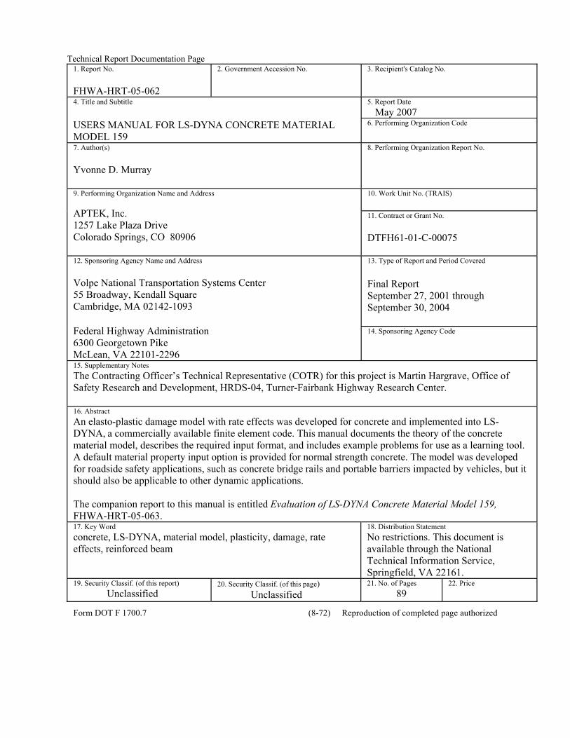
Technical Report Documentation Page 1. Report No. FHWA-HRT-05-062

2. Government Accession No. 3. Recipient's Catalog No.

5. Report Date May 2007

4. Title and Subtitle USERS MANUAL FOR LS-DYNA CONCRETE MATERIAL MODEL 159

6. Performing Organization Code

7. Author(s) Yvonne D. Murray

8. Performing Organization Report No.

10. Work Unit No. (TRAIS)

9. Performing Organization Name and Address APTEK, Inc. 1257 Lake Plaza Drive Colorado Springs, CO 80906

11. Contract or Grant No. DTFH61-01-C-00075

13. Type of Report and Period Covered Final Report September 27, 2001 through September 30, 2004

12. Sponsoring Agency Name and Address Volpe National Transportation Systems Center 55 Broadway, Kendall Square Cambridge, MA 02142-1093 Federal Highway Administration 6300 Georgetown Pike McLean, VA 22101-2296

14. Sponsoring Agency Code

15. Supplementary Notes The Contracting Officer’s Technical Representative (COTR) for this project is Martin Hargrave, Office of Safety Research and Development, HRDS-04, Turner-Fairbank Highway Research Center. 16. Abstract An elasto-plastic damage model with rate effects was developed for concrete and implemented into LS-DYNA, a commercially available finite element code. This manual documents the theory of the concrete material model, describes the required input format, and includes example problems for use as a learning tool. A default material property input option is provided for normal strength concrete. The model was developed for roadside safety applications, such as concrete bridge rails and portable barriers impacted by vehicles, but it should also be applicable to other dynamic applications. The companion report to this manual is entitled Evaluation of LS-DYNA Concrete Material Model 159, FHWA-HRT-05-063. 17. Key Word concrete, LS-DYNA, material model, plasticity, damage, rate effects, reinforced beam

18. Distribution Statement No restrictions. This document is available through the National Technical Information Service, Springfield, VA 22161.

19. Security Classif. (of this report) Unclassified

20. Security Classif. (of this page) Unclassified

21. No. of Pages 89

22. Price

Form DOT F 1700.7 (8-72) Reproduction of completed page authorized

ii

SI* (MODERN METRIC) CONVERSION FACTORS APPROXIMATE CONVERSIONS TO SI UNITS

Symbol When You Know Multiply By To Find Symbol LENGTH

in inches 25.4 millimeters mm ft feet 0.305 meters m yd yards 0.914 meters m mi miles 1.61 kilometers km

AREA in2 square inches 645.2 square millimeters mm2

ft2 square feet 0.093 square meters m2

yd2 square yard 0.836 square meters m2

ac acres 0.405 hectares hami2 square miles 2.59 square kilometers km2

VOLUME fl oz fluid ounces 29.57 milliliters mL gal gallons 3.785 liters L ft3 cubic feet 0.028 cubic meters m3

yd3 cubic yards 0.765 cubic meters m3

NOTE: volumes greater than 1000 L shall be shown in m3

MASS oz ounces 28.35 grams glb pounds 0.454 kilograms kgT short tons (2000 lb) 0.907 megagrams (or "metric ton") Mg (or "t")

TEMPERATURE (exact degrees) oF Fahrenheit 5 (F-32)/9 Celsius oC

or (F-32)/1.8 ILLUMINATION

fc foot-candles 10.76 lux lxfl foot-Lamberts 3.426 candela/m2 cd/m2

FORCE and PRESSURE or STRESS lbf poundforce 4.45 newtons N lbf/in2 poundforce per square inch 6.89 kilopascals kPa

APPROXIMATE CONVERSIONS FROM SI UNITS Symbol When You Know Multiply By To Find Symbol

LENGTHmm millimeters 0.039 inches in m meters 3.28 feet ft m meters 1.09 yards yd km kilometers 0.621 miles mi

AREA mm2 square millimeters 0.0016 square inches in2

m2 square meters 10.764 square feet ft2

m2 square meters 1.195 square yards yd2

ha hectares 2.47 acres ackm2 square kilometers 0.386 square miles mi2

VOLUME mL milliliters 0.034 fluid ounces fl oz L liters 0.264 gallons gal m3 cubic meters 35.314 cubic feet ft3

m3 cubic meters 1.307 cubic yards yd3

MASS g grams 0.035 ounces ozkg kilograms 2.202 pounds lbMg (or "t") megagrams (or "metric ton") 1.103 short tons (2000 lb) T

TEMPERATURE (exact degrees) oC Celsius 1.8C+32 Fahrenheit oF

ILLUMINATION lx lux 0.0929 foot-candles fc cd/m2 candela/m2 0.2919 foot-Lamberts fl

FORCE and PRESSURE or STRESS N newtons 0.225 poundforce lbf kPa kilopascals 0.145 poundforce per square inch lbf/in2

*SI is the symbol for th International System of Units. Appropriate rounding should be made to comply with Section 4 of ASTM E380. e(Revised March 2003)

iii

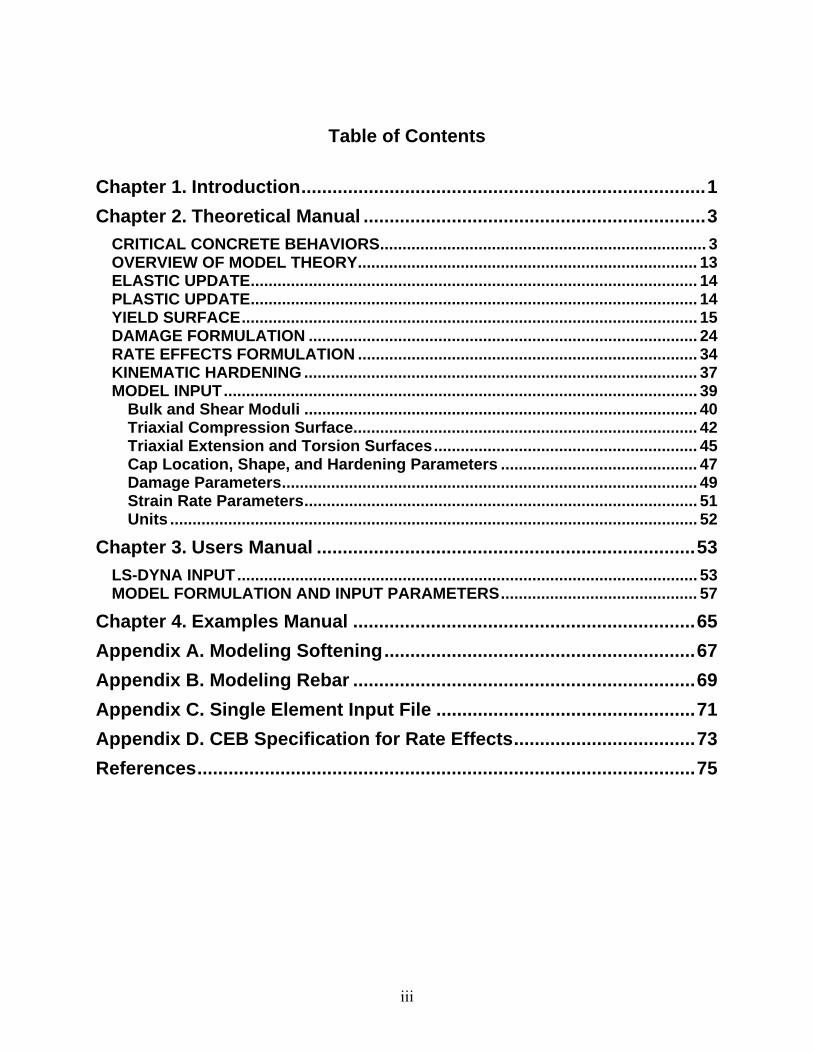
Table of Contents

Chapter 1. Introduction..............................................................................1 Chapter 2. Theoretical Manual ..................................................................3

CRITICAL CONCRETE BEHAVIORS......................................................................... 3 OVERVIEW OF MODEL THEORY............................................................................ 13 ELASTIC UPDATE.................................................................................................... 14 PLASTIC UPDATE.................................................................................................... 14 YIELD SURFACE...................................................................................................... 15 DAMAGE FORMULATION ....................................................................................... 24 RATE EFFECTS FORMULATION ............................................................................ 34 KINEMATIC HARDENING ........................................................................................ 37 MODEL INPUT.......................................................................................................... 39

Bulk and Shear Moduli ........................................................................................ 40 Triaxial Compression Surface............................................................................. 42 Triaxial Extension and Torsion Surfaces........................................................... 45 Cap Location, Shape, and Hardening Parameters ............................................ 47 Damage Parameters............................................................................................. 49 Strain Rate Parameters........................................................................................ 51 Units ...................................................................................................................... 52

Chapter 3. Users Manual .........................................................................53 LS-DYNA INPUT....................................................................................................... 53 MODEL FORMULATION AND INPUT PARAMETERS............................................ 57

Chapter 4. Examples Manual ..................................................................65 Appendix A. Modeling Softening............................................................67 Appendix B. Modeling Rebar ..................................................................69 Appendix C. Single Element Input File ..................................................71 Appendix D. CEB Specification for Rate Effects...................................73 References................................................................................................75

iv

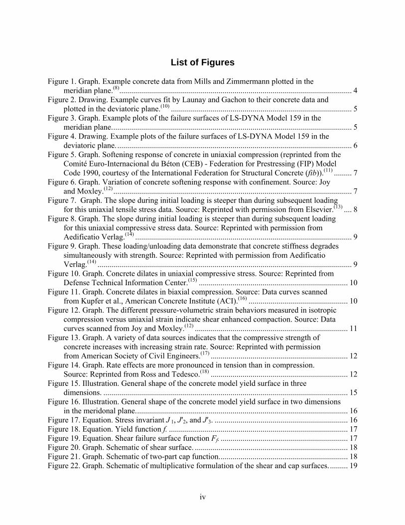
List of Figures

Figure 1. Graph. Example concrete data from Mills and Zimmermann plotted in the

meridian plane.(8)..................................................................................................................... 4 Figure 2. Drawing. Example curves fit by Launay and Gachon to their concrete data and

plotted in the deviatoric plane.(10) ........................................................................................... 5 Figure 3. Graph. Example plots of the failure surfaces of LS-DYNA Model 159 in the

meridian plane......................................................................................................................... 5 Figure 4. Drawing. Example plots of the failure surfaces of LS-DYNA Model 159 in the

deviatoric plane....................................................................................................................... 6 Figure 5. Graph. Softening response of concrete in uniaxial compression (reprinted from the

Comité Euro-Internacional du Béton (CEB) - Federation for Prestressing (FIP) Model Code 1990, courtesy of the International Federation for Structural Concrete (fib)).(11) ......... 7

Figure 6. Graph. Variation of concrete softening response with confinement. Source: Joy and Moxley.(12) ........................................................................................................................ 7

Figure 7. Graph. The slope during initial loading is steeper than during subsequent loading for this uniaxial tensile stress data. Source: Reprinted with permission from Elsevier.(13) .... 8

Figure 8. Graph. The slope during initial loading is steeper than during subsequent loading for this uniaxial compressive stress data. Source: Reprinted with permission from Aedificatio Verlag.(14) ............................................................................................................. 9

Figure 9. Graph. These loading/unloading data demonstrate that concrete stiffness degrades simultaneously with strength. Source: Reprinted with permission from Aedificatio Verlag.(14) ................................................................................................................................ 9

Figure 10. Graph. Concrete dilates in uniaxial compressive stress. Source: Reprinted from Defense Technical Information Center.(15) ........................................................................... 10

Figure 11. Graph. Concrete dilates in biaxial compression. Source: Data curves scanned from Kupfer et al., American Concrete Institute (ACI).(16) .................................................. 10

Figure 12. Graph. The different pressure-volumetric strain behaviors measured in isotropic compression versus uniaxial strain indicate shear enhanced compaction. Source: Data curves scanned from Joy and Moxley.(12) ............................................................................. 11

Figure 13. Graph. A variety of data sources indicates that the compressive strength of concrete increases with increasing strain rate. Source: Reprinted with permission from American Society of Civil Engineers.(17) ..................................................................... 12

Figure 14. Graph. Rate effects are more pronounced in tension than in compression. Source: Reprinted from Ross and Tedesco.(18) ..................................................................... 12

Figure 15. Illustration. General shape of the concrete model yield surface in three dimensions. ........................................................................................................................... 15

Figure 16. Illustration. General shape of the concrete model yield surface in two dimensions in the meridonal plane........................................................................................................... 16

Figure 17. Equation. Stress invariant J 1, J′2, and J′3. ................................................................... 16 Figure 18. Equation. Yield function f. .......................................................................................... 17 Figure 19. Equation. Shear failure surface function Ff. ................................................................ 17 Figure 20. Graph. Schematic of shear surface. ............................................................................. 18 Figure 21. Graph. Schematic of two-part cap function................................................................. 18 Figure 22. Graph. Schematic of multiplicative formulation of the shear and cap surfaces.......... 19

v

Figure 23. Equation. Cap failure surface function Fc. .................................................................. 19 Figure 24. Equation. L of kappa.................................................................................................... 20 Figure 25. Equation. Simple cap failure surface function Fc........................................................ 20 Figure 26. Equation. X as a function of kappa. .......................................................................... 20 Figure 27. Equation. Plastic volume strain ε p

v. ............................................................................ 20 Figure 28. Illustration. Example two- and three-invariant shapes of the concrete model in

the deviatoric plane. .............................................................................................................. 21 Figure 29. Equation. Angle beta hat in the deviatoric plane......................................................... 22 Figure 30. Equation. Relationship between beta hat and J hat. .................................................... 22 Figure 31. Equation. Rubin scaling function ℜ. ........................................................................... 22 Figure 32. Equation. Most general form for Q1 and Q2. ............................................................... 23 Figure 33. Equation. Mohr-Coulomb form for Q1, Q2.................................................................. 23 Figure 34. Equation. Willam-Warnke form for Q1. ...................................................................... 23 Figure 35. Equation. Damaged stress σ dij..................................................................................... 24 Figure 36. Graph. This cap model simulation demonstrates strain softening and modulus

reduction. .............................................................................................................................. 25 Figure 37. Equation. Brittle damage threshold τb. ........................................................................ 25 Figure 38. Equation. Ductile damage threshold τd........................................................................ 25 Figure 39. Equation. Viscoplastic damage threshold r0................................................................ 26 Figure 40. Equation. Incremental damage threshold, small rn+1................................................... 26 Figure 41. Equation. Brittle damage small d of tau. ..................................................................... 27 Figure 42. Equation. Ductile damage small d of tau..................................................................... 27 Figure 43. Equation. Variation of dmax with stress invariant ratio. ............................................. 27 Figure 44. Equation. Variation of dmax with rate effects............................................................. 28 Figure 45. Schematic representation of four stress paths and their stress invariant ratios. .......... 28 Figure 46. Equation. Reduction of A with confinement. .............................................................. 28 Figure 47. Equation. Fracture energy integral for Gf. ................................................................... 29 Figure 48. Equation. Brittle damage fracture energy Gf. .............................................................. 30 Figure 49. Equation. Brittle damage threshold difference τ minus small r0b................................ 30 Figure 50. Equation. Brittle softening parameter C. ..................................................................... 30 Figure 51. Equation. Ductile damage fracture energy Gf. ............................................................ 30 Figure 52. Equation. Ductile damage threshold difference τ − r0d. .............................................. 30 Figure 53. Equation. Ductile softening parameter A..................................................................... 31 Figure 54. Equation. Brittle damage threshold Gf Brittle................................................................. 32 Figure 55. Equation. Ductile damage threshold Gf

Ductile. ............................................................. 32 Figure 56. Equation. The fracture energy with rate effects, Gvp

f . ................................................ 32 Figure 57. Equation. Default damage recovery of d of τt ............................................................. 33 Figure 58. Equation. Optional damage recovery of d of τt. .......................................................... 33 Figure 59. Equation. Viscoplastic stress update for σvp

ij. ............................................................. 34 Figure 60. Equation. Two-parameter η. ........................................................................................ 34 Figure 61. Equation. Dynamic strengths, f ′T dynamic, and f ′C dynamic. ............................................. 35 Figure 62. Equation. Effective strain rate ............................................................................... 35 Figure 63. Equation. Variation of fluidity parameter η in tension................................................ 36 Figure 64. Equation. Variation of fluidity parameter η in compression. ...................................... 36 Figure 65. Equation. Effective fluidity parameters, ηt, ηc, and η s. .............................................. 36 Figure 66. Equation. Overstress limit of η. .................................................................................. 37

vi

Figure 67. Equation. Back stress α ij n + 1...................................................................................... 37 Figure 68. Equation. Updated stress with hardening, σP

ij n+1....................................................... 37 Figure 69. Equation. Incremental back stress, Δαij. ..................................................................... 38 Figure 70. Equation. Brittle rate of translation CH

Brittle. .............................................................. 38 Figure 71. Equation. Ductile rate of translation CH

Ductile............................................................. 38 Figure 72. Equation. The limiting function Gα. ........................................................................... 39 Figure 73. Equation. Modified shear failure surface, Ff. ............................................................. 39 Figure 74. Equation. Default Young’s modulus E....................................................................... 40 Figure 75. Equation. Shear and bulk moduli, G and K. ............................................................... 40 Figure 76. Equation. ACI Young’s modulus, Ec.......................................................................... 41 Figure 77. Equation. Reduced ACI Young’s modulus, Ec........................................................... 41 Figure 78. Equation. TXC Strength. ............................................................................................ 43 Figure 79. Equation. Interpolation parameter P........................................................................... 43 Figure 80. Equation. Most general form for Q1, Q2..................................................................... 45 Figure 81. Graph. This isotropic compression simulation demonstrates how the cap

parameters set the shape of the pressure-volumetric strain curve......................................... 49 Figure 82. Equation. The default fracture energy GF. ................................................................. 49 Figure 83. Graph. Approximate tensile and compressive dynamic increase factors for

default concrete model behavior........................................................................................... 52 Figure 84. Illustration. General shape of the concrete model yield surface in two dimensions. .. 57 Figure 85. Equation. Three stress invariants, J1, J′2, J′3................................................................ 58 Figure 86. Equation. Plasticity yield function f. ........................................................................... 58 Figure 87. Equation. Shear surface function Ff. ........................................................................... 58 Figure 88. Equation. Most general form for scaling functions Q1, Q2.......................................... 59 Figure 89. Equation. Cap surface function, Fc.............................................................................. 59 Figure 90. Equation. Definition of L of kappa.............................................................................. 59 Figure 91. Equation. Pressure invariant X as a function of kappa. .............................................. 59 Figure 92. Equation. Plastic volume strain hardening rule, ε pv................................................... 60 Figure 93. Equation. Transformation of viscoplastic stress to damaged stress, σd

ij..................... 60 Figure 94. Equation. Ductile damage accumulation, τ d. ............................................................. 61 Figure 95. Equation. Brittle damage accumulation, τb. ............................................................... 61 Figure 96. Equation. Brittle damage, d of τb................................................................................ 61 Figure 97. Equation. Ductile damage, d of τd. ............................................................................. 61 Figure 98. Equation. Reduction of A with confinement. ............................................................. 61 Figure 99. Equation. Brittle and ductile damage thresholds, Gf. ................................................. 62 Figure 100. Equation. Viscoplastic stress, σvp

ij............................................................................. 62 Figure 101. Equation. Variation of the fluidity parameter η in tension and compression. ........... 63 Figure 102. Definition of effective strain rate. ............................................................................. 63 Figure 103. Equation. Overstress limit of η. ................................................................................. 63 Figure 104. Equation. Fracture energy with rate effects, ..................................................... 64 Figure 105. Computer printout. Example concrete model input for default material property

input (option mat_CSCM_concrete)..................................................................................... 65 Figure 106. Computer printout. Example concrete model input for user-specified material

property input (option MAT_CSCM)................................................................................... 66 Figure 107. Graph. Example single element stress-strain results for 30 MPa (4,351 psi)

concrete with 19-mm (0.75-inch) maximum aggregate size. ............................................... 66

vii

Figure 108. Equation. Old generic damage, small d of τ. ............................................................ 67 Figure 109. Equation. New generic damage, small d of τ. .......................................................... 67 Figure 110. Graph. Behavior of the original softening function................................................... 68 Figure 111. Graph. Behavior of the updated softening function. ................................................. 68 Figure 112. Graph. Rebar yields in a ductile manner at a quasi-static rate of 0.0054/s.

Source: U.S. Army Engineer Waterways Experiment Station.(29) ........................................ 69 Figure 113. Graph. Rebar exhibits rate effects at a strain rate of 4/s. Source: U.S. Army

Engineer Waterways Experiment Station.(29)........................................................................ 69 Figure 114. Equation. CEB tensile strength dynamic increase factor, DIFten. ............................ 73 Figure 115. Equation. CEB compressive strength dynamic increase factor, DIFcomp. ................ 73 Figure 116. Graph. Dynamic increase factors specified in CEB. ................................................ 74

viii

List of Tables

Table 1. These default bulk and shear moduli of concrete are derived from the formula for Young’s modulus provided in CEB...................................................................................... 41

Table 2. These bulk and shear moduli for concrete are derived from a formula for Young’s modulus suggested by ACI Code Committee....................................................................... 42

Table 3. Approximate strength measurements used to set default TXC yield surface parameters. ............................................................................................................................ 43

Table 4. TXC yield surface input parameters as a function of unconfined compression strength.................................................................................................................................. 44

Table 5. Quadratic equation coefficients which set the default TXC, TOR, and TXE yield surface parameters as a function of unconfined compression strength................................. 45

Table 6. TOR yield surface input parameters as a function of unconfined compression strength.................................................................................................................................. 46

Table 7. TXE yield surface input parameters as a function of unconfined compression strength.................................................................................................................................. 47

Table 8. Cap shape, location, and hardening parameters as a function of unconfined compression strength. ........................................................................................................... 48

Table 9. Coefficients for the fracture energy equation. ................................................................ 50 Table 10. Tensile fracture energies tabulated in CEB as a function of concrete strength. ........... 50 Table 11. Example load curve for modeling rebar strain rate effects with LS-DYNA Material

Model #24. ............................................................................................................................ 70

ix

Glossary of Symbols

a a0 a1 a2 Rubin function internal parameters

A B C D softening parameters (compression and tension)

AP BP CP quadratic equation coefficients

b b0 b1 b2 Rubin function internal parameters

Bs term used in one rate effects formula

CH hardening rate parameter

d d b d d scalar damage parameter (general, brittle, ductile)

dm maximum of brittle and ductile scalar damage parameters

dmax maximum damage allowed to accumulate

D1 D2 cap linear and quadratic shape parameters E Ec Es Young’s modulus (general, concrete, steel) f yield surface function

f* trial elastic yield surface function

Ff shear failure surface

Fc hardening cap surface

G shear modulus

Gα hardening model translational limit function for shear surface

Gft Gfc Gfs fracture energies (tension, compression, shear)

J1 first invariant of the stress tensor

J ′2 J ′3 second and third invariants of the deviatoric stress tensor

J1T J ′2

T J ′3T trial elastic stress invariants

J1P J ′2

P J ′3P inviscid elastic stress invariants

normalized invariant of the deviatoric stress tensor

K bulk modulus

L element length

NH hardening initiation

nt nc rate effects fluidity parameters (tension, compression)

Nt NC rate effects power parameters (tension and compression)

P pressure

x

Q1 Q2 Rubin scaling functions for torsion and triaxial extension

ℜ Rubin strength reduction factor

R cap aspect ratio rS initial damage before activation of rate effects

r0 r0b r0d initial damage threshold (general, brittle, ductile)

Sij deviatoric stress tensor

W maximum plastic volume compaction

x x0 instantaneous displacement and displacement at peak strength

X X0 current cap location and initial cap location y integrand of dilogarithm function αij Δαij hardening model back stress and incremental back stress tensors

α α1 α2 shear surface constant term (compression, torsion, extension)

αs term used in one rate effects formula

β β1 β2 shear surface exponent (compression, torsion, extension)

β̂ angle in deviatoric plane (invariant)

λΔ plasticity consistency parameter

Δt time step increment

εij Δεij strain tensor and strain increments

ε& ε&Δ effective strain rate and effective strain rate increment

0ε& term used in one rate effects equation

εmax maximum principal strain εx εy εz εxy εyz εxz strain components

εv volumetric strain

ε pv plastic volumetric strain

γ viscoplastic interpolation parameter

γ s term used in one rate effects formula

η ηt ηc ηs rate effects fluidity parameters (general, tension, compression, shear)

xi

η0t nt rate effects input parameters in uniaxial tension stress

η0c nc rate effects input parameters in uniaxial compressive stress κ κΤ κP κ0 cap hardening parameters (general, trial elastic, inviscid, initial)

λ λ1 λ2 shear surface nonlinear term (compression, torsion, extension) ν Poisson’s ratio

θ θ1 θ2 shear surface linear term (compression, torsion, extension)

ρ ρc ρs density (general, concrete, steel)

ρt ρc ρs meridians (tensile, compressive, shear)

σ σ T a stress component (general, trail elastic)

σ x σ r axial and radial stresses measured in triaxial compression tests

σ vp σ d stress components calculated without and with damage

Pij

Tij

vpij σ σ σ stress tensors (viscoplastic, trial elastic, plastic)

σ 1 σ 2 σ 3 principal stress components

τ b τ d instantaneous strain energy-type terms for damage accumulation

xii

Acronyms and Abbreviations ACI American Concrete Institute

CEB Comité Euro-Internacional du Béton

CSCM continuous surface cap model

DIF dynamic increase factor

FIP Federation for Prestressing

NCHRP National Cooperative Highway Research Program

TOR torsion

TXC triaxial compression

TXE triaxial extension

1

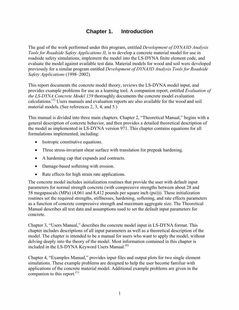
Chapter 1. Introduction

The goal of the work performed under this program, entitled Development of DYNA3D Analysis Tools for Roadside Safety Applications II, is to develop a concrete material model for use in roadside safety simulations, implement the model into the LS-DYNA finite element code, and evaluate the model against available test data. Material models for wood and soil were developed previously for a similar program entitled Development of DYNA3D Analysis Tools for Roadside Safety Applications (1998–2002). This report documents the concrete model theory, reviews the LS-DYNA model input, and provides example problems for use as a learning tool. A companion report, entitled Evaluation of the LS-DYNA Concrete Model 159 thoroughly documents the concrete model evaluation calculations.(1) Users manuals and evaluation reports are also available for the wood and soil material models. (See references 2, 3, 4, and 5.) This manual is divided into three main chapters. Chapter 2, “Theoretical Manual,” begins with a general description of concrete behavior, and then provides a detailed theoretical description of the model as implemented in LS-DYNA version 971. This chapter contains equations for all formulations implemented, including:

• Isotropic constitutive equations.

• Three stress-invariant shear surface with translation for prepeak hardening.

• A hardening cap that expands and contracts.

• Damage-based softening with erosion.

• Rate effects for high strain rate applications.

The concrete model includes initialization routines that provide the user with default input parameters for normal strength concrete (with compressive strengths between about 28 and 58 megapascals (MPa) (4,061 and 8,412 pounds per square inch (psi))). These initialization routines set the required strengths, stiffnesses, hardening, softening, and rate effects parameters as a function of concrete compressive strength and maximum aggregate size. The Theoretical Manual describes all test data and assumptions used to set the default input parameters for concrete. Chapter 3, “Users Manual,” describes the concrete model input in LS-DYNA format. This chapter includes descriptions of all input parameters as well as a theoretical description of the model. The chapter is intended to be a manual for users who want to apply the model, without delving deeply into the theory of the model. Most information contained in this chapter is included in the LS-DYNA Keyword Users Manual.(6) Chapter 4, “Examples Manual,” provides input files and output plots for two single element simulations. These example problems are designed to help the user become familiar with applications of the concrete material model. Additional example problems are given in the companion to this report.(1)

3

Chapter 2. Theoretical Manual

This chapter begins with an overview of concrete behavior, followed by a detailed description of the formulation of concrete material model 159 in LS-DYNA. Equations are provided for each feature of the model (elasticity, plasticity, hardening, damage, and rate effects). The chapter then describes the model input properties and the basis for their default values.

CRITICAL CONCRETE BEHAVIORS

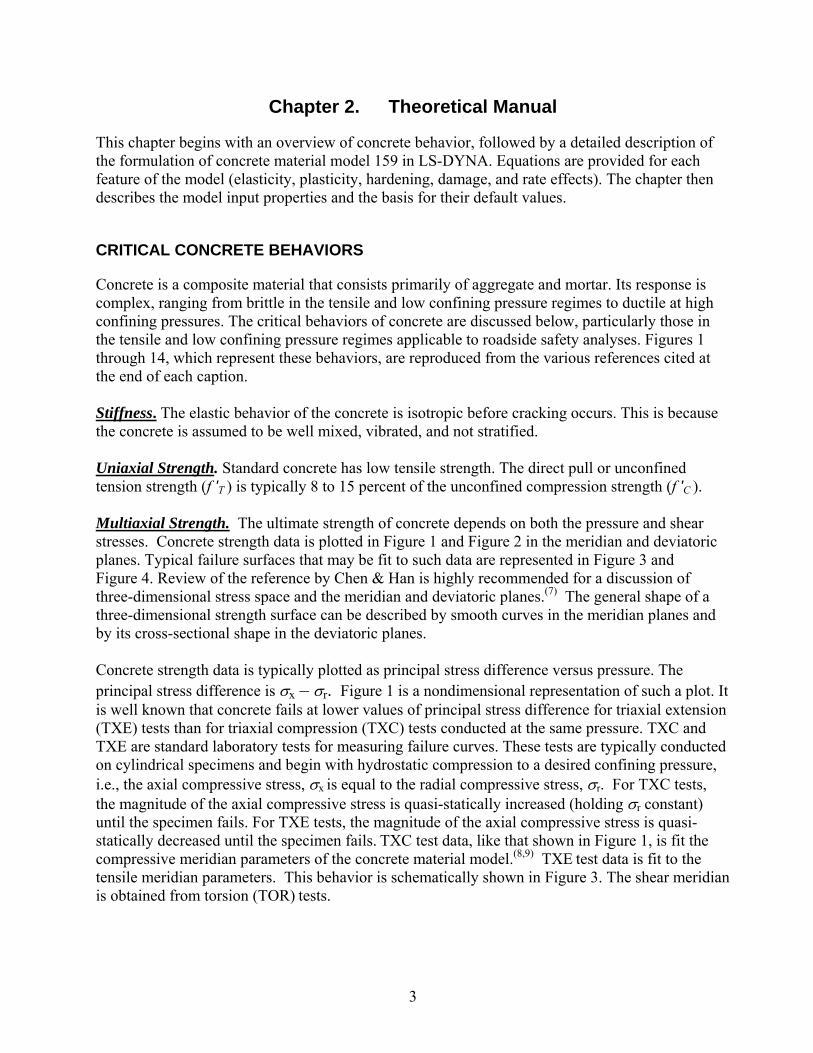
Concrete is a composite material that consists primarily of aggregate and mortar. Its response is complex, ranging from brittle in the tensile and low confining pressure regimes to ductile at high confining pressures. The critical behaviors of concrete are discussed below, particularly those in the tensile and low confining pressure regimes applicable to roadside safety analyses. Figures 1 through 14, which represent these behaviors, are reproduced from the various references cited at the end of each caption. Stiffness. The elastic behavior of the concrete is isotropic before cracking occurs. This is because the concrete is assumed to be well mixed, vibrated, and not stratified. Uniaxial Strength. Standard concrete has low tensile strength. The direct pull or unconfined tension strength (f 'T ) is typically 8 to 15 percent of the unconfined compression strength (f 'C ). Multiaxial Strength. The ultimate strength of concrete depends on both the pressure and shear stresses. Concrete strength data is plotted in Figure 1 and Figure 2 in the meridian and deviatoric planes. Typical failure surfaces that may be fit to such data are represented in Figure 3 and Figure 4. Review of the reference by Chen & Han is highly recommended for a discussion of three-dimensional stress space and the meridian and deviatoric planes.(7) The general shape of a three-dimensional strength surface can be described by smooth curves in the meridian planes and by its cross-sectional shape in the deviatoric planes. Concrete strength data is typically plotted as principal stress difference versus pressure. The principal stress difference is σx – σr. Figure 1 is a nondimensional representation of such a plot. It is well known that concrete fails at lower values of principal stress difference for triaxial extension (TXE) tests than for triaxial compression (TXC) tests conducted at the same pressure. TXC and TXE are standard laboratory tests for measuring failure curves. These tests are typically conducted on cylindrical specimens and begin with hydrostatic compression to a desired confining pressure, i.e., the axial compressive stress, σx is equal to the radial compressive stress, σr. For TXC tests, the magnitude of the axial compressive stress is quasi-statically increased (holding σr constant) until the specimen fails. For TXE tests, the magnitude of the axial compressive stress is quasi-statically decreased until the specimen fails. TXC test data, like that shown in Figure 1, is fit the compressive meridian parameters of the concrete material model.(8,9) TXE test data is fit to the tensile meridian parameters. This behavior is schematically shown in Figure 3. The shear meridian is obtained from torsion (TOR) tests.

4

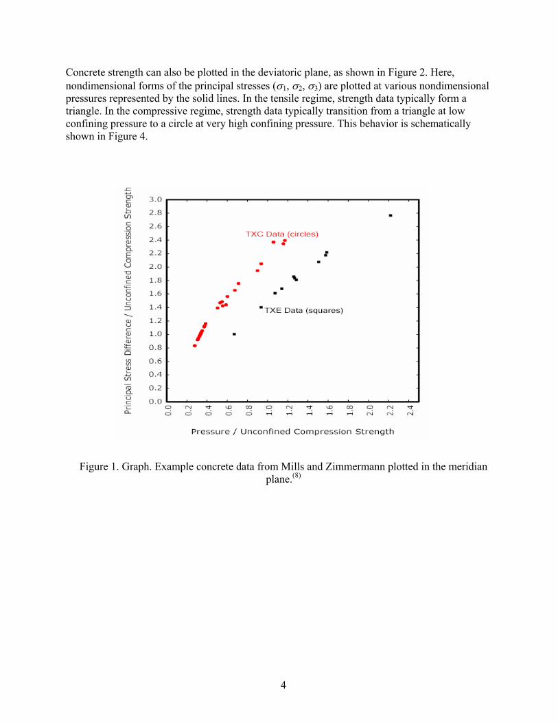
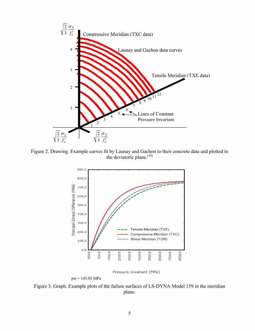
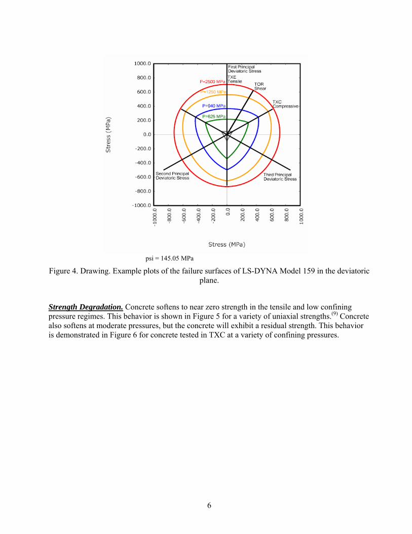
Concrete strength can also be plotted in the deviatoric plane, as shown in Figure 2. Here, nondimensional forms of the principal stresses (σ1, σ2, σ3) are plotted at various nondimensional pressures represented by the solid lines. In the tensile regime, strength data typically form a triangle. In the compressive regime, strength data typically transition from a triangle at low confining pressure to a circle at very high confining pressure. This behavior is schematically shown in Figure 4.

Figure 1. Graph. Example concrete data from Mills and Zimmermann plotted in the meridian plane.(8)

5

Figure 2. Drawing. Example curves fit by Launay and Gachon to their concrete data and plotted in the deviatoric plane.(10)

psi = 145.05 MPa

Figure 3. Graph. Example plots of the failure surfaces of LS-DYNA Model 159 in the meridian plane.

1 2

3 4 5

6 7

8 9 10 11 12

Lines of Constant Pressure Invariant

Compressive Meridian (TXC data)

Tensile Meridian (TXE data)

cf ′2

32 σ

cf ′1

32 σ

cf ′3

32 σ

Launay and Gachon data curves 4

3

2

1

6

psi = 145.05 MPa

Figure 4. Drawing. Example plots of the failure surfaces of LS-DYNA Model 159 in the deviatoric plane.

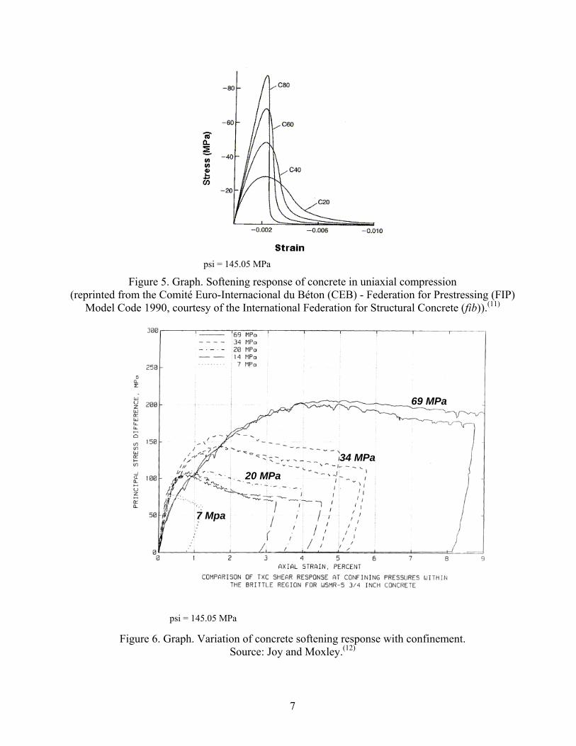
Strength Degradation. Concrete softens to near zero strength in the tensile and low confining pressure regimes. This behavior is shown in Figure 5 for a variety of uniaxial strengths.(9) Concrete also softens at moderate pressures, but the concrete will exhibit a residual strength. This behavior is demonstrated in Figure 6 for concrete tested in TXC at a variety of confining pressures.

7

psi = 145.05 MPa

Figure 5. Graph. Softening response of concrete in uniaxial compression (reprinted from the Comité Euro-Internacional du Béton (CEB) - Federation for Prestressing (FIP)

Model Code 1990, courtesy of the International Federation for Structural Concrete (fib)).(11)

psi = 145.05 MPa

Figure 6. Graph. Variation of concrete softening response with confinement. Source: Joy and Moxley.(12)

14 MPa 7 Mpa

20 MPa

34 MPa

69 MPa

8

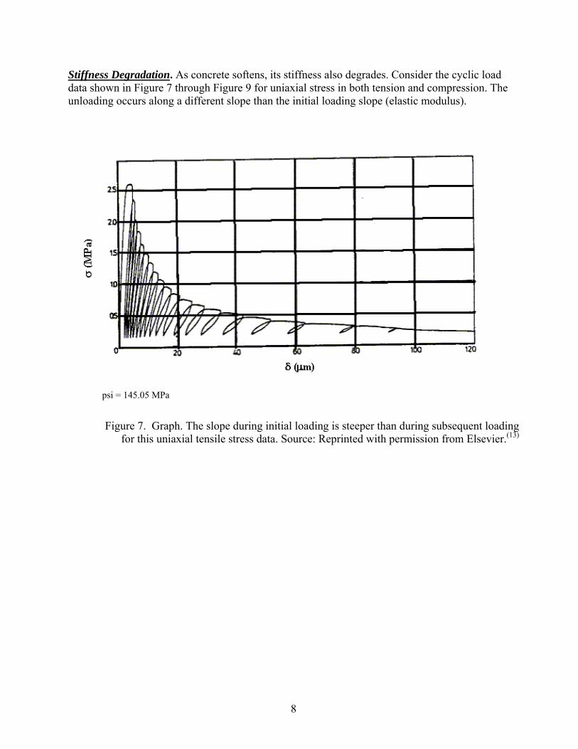
Stiffness Degradation. As concrete softens, its stiffness also degrades. Consider the cyclic load data shown in Figure 7 through Figure 9 for uniaxial stress in both tension and compression. The unloading occurs along a different slope than the initial loading slope (elastic modulus).

psi = 145.05 MPa

Figure 7. Graph. The slope during initial loading is steeper than during subsequent loading for this uniaxial tensile stress data. Source: Reprinted with permission from Elsevier.(13)

9

Figure 8. Graph. The slope during initial loading is steeper than during subsequent loading

for this uniaxial compressive stress data. Source: Reprinted with permission from Aedificatio Verlag.(14)

Figure 9. Graph. These loading/unloading data demonstrate that concrete stiffness degrades

simultaneously with strength. Source: Reprinted with permission from Aedificatio Verlag.(14)

10

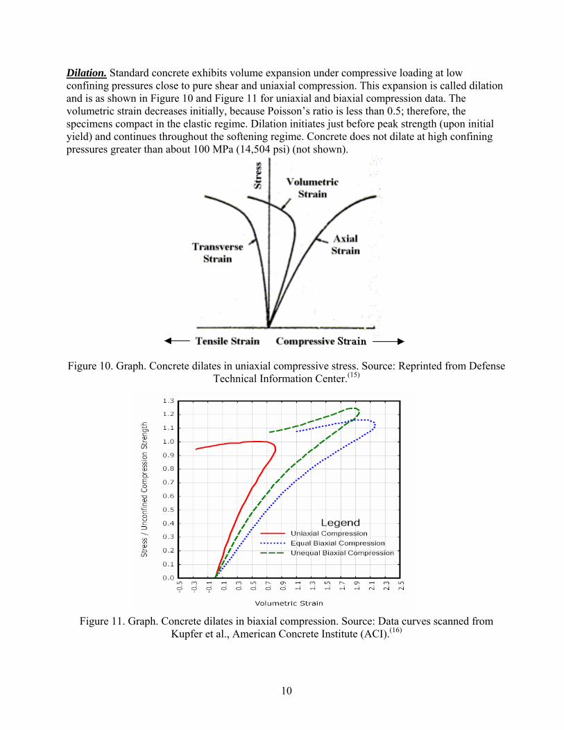
Dilation. Standard concrete exhibits volume expansion under compressive loading at low confining pressures close to pure shear and uniaxial compression. This expansion is called dilation and is as shown in Figure 10 and Figure 11 for uniaxial and biaxial compression data. The volumetric strain decreases initially, because Poisson’s ratio is less than 0.5; therefore, the specimens compact in the elastic regime. Dilation initiates just before peak strength (upon initial yield) and continues throughout the softening regime. Concrete does not dilate at high confining pressures greater than about 100 MPa (14,504 psi) (not shown).

Figure 10. Graph. Concrete dilates in uniaxial compressive stress. Source: Reprinted from Defense

Technical Information Center.(15)

Figure 11. Graph. Concrete dilates in biaxial compression. Source: Data curves scanned from Kupfer et al., American Concrete Institute (ACI).(16)

11

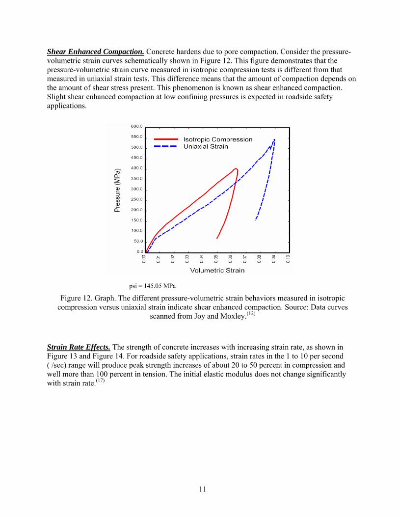
Shear Enhanced Compaction. Concrete hardens due to pore compaction. Consider the pressure-volumetric strain curves schematically shown in Figure 12. This figure demonstrates that the pressure-volumetric strain curve measured in isotropic compression tests is different from that measured in uniaxial strain tests. This difference means that the amount of compaction depends on the amount of shear stress present. This phenomenon is known as shear enhanced compaction. Slight shear enhanced compaction at low confining pressures is expected in roadside safety applications.

psi = 145.05 MPa

Figure 12. Graph. The different pressure-volumetric strain behaviors measured in isotropic compression versus uniaxial strain indicate shear enhanced compaction. Source: Data curves

scanned from Joy and Moxley.(12)

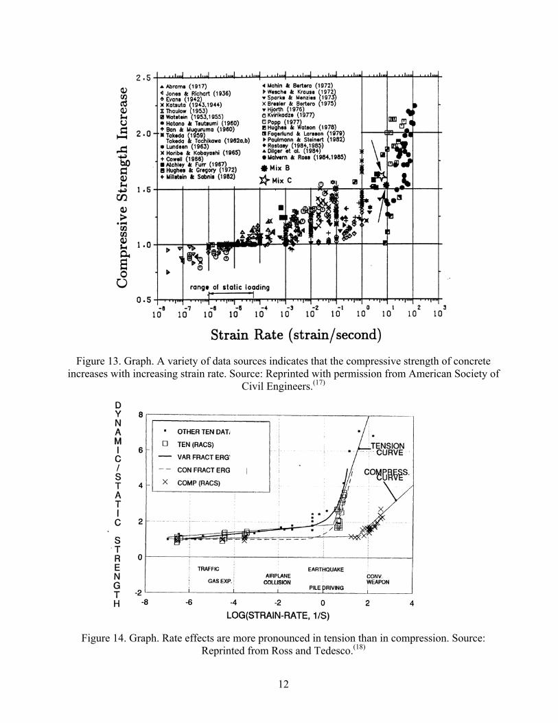
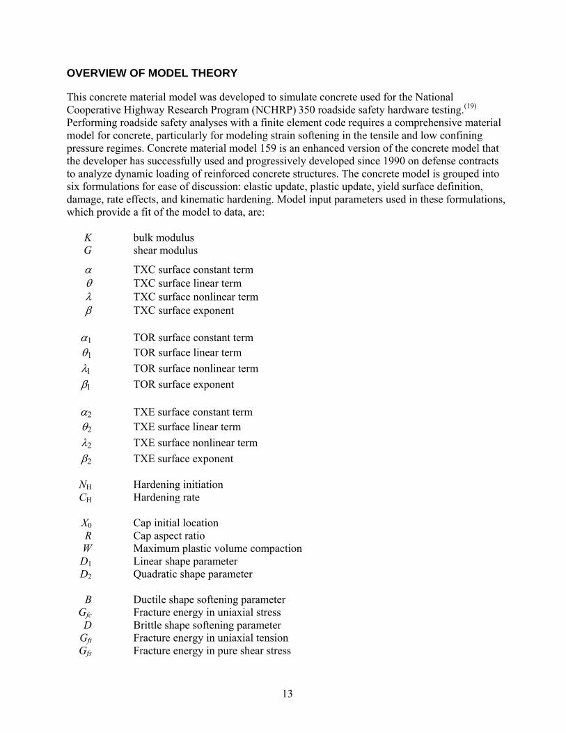
Strain Rate Effects. The strength of concrete increases with increasing strain rate, as shown in Figure 13 and Figure 14. For roadside safety applications, strain rates in the 1 to 10 per second ( /sec) range will produce peak strength increases of about 20 to 50 percent in compression and well more than 100 percent in tension. The initial elastic modulus does not change significantly with strain rate.(17)

12

Figure 13. Graph. A variety of data sources indicates that the compressive strength of concrete

increases with increasing strain rate. Source: Reprinted with permission from American Society of Civil Engineers.(17)

Figure 14. Graph. Rate effects are more pronounced in tension than in compression. Source:

Reprinted from Ross and Tedesco.(18)

13

OVERVIEW OF MODEL THEORY

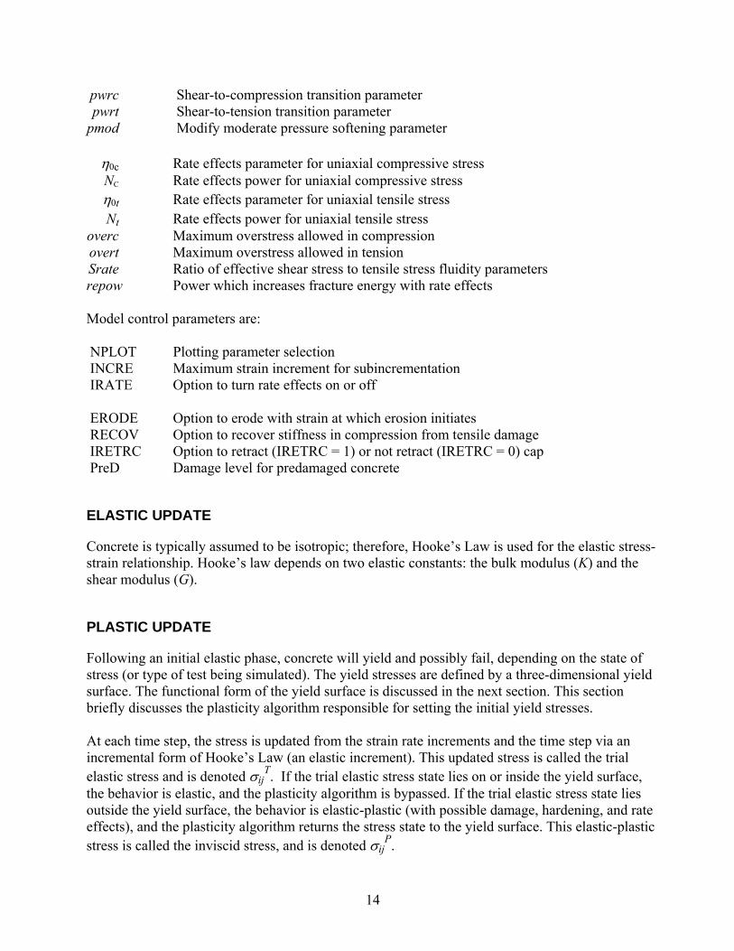
This concrete material model was developed to simulate concrete used for the National Cooperative Highway Research Program (NCHRP) 350 roadside safety hardware testing.(19) Performing roadside safety analyses with a finite element code requires a comprehensive material model for concrete, particularly for modeling strain softening in the tensile and low confining pressure regimes. Concrete material model 159 is an enhanced version of the concrete model that the developer has successfully used and progressively developed since 1990 on defense contracts to analyze dynamic loading of reinforced concrete structures. The concrete model is grouped into six formulations for ease of discussion: elastic update, plastic update, yield surface definition, damage, rate effects, and kinematic hardening. Model input parameters used in these formulations, which provide a fit of the model to data, are: K bulk modulus G shear modulus

α TXC surface constant term θ TXC surface linear term λ TXC surface nonlinear term β TXC surface exponent α1 TOR surface constant term θ1 TOR surface linear term λ1 TOR surface nonlinear term β1 TOR surface exponent α2 TXE surface constant term θ2 TXE surface linear term λ2 TXE surface nonlinear term β2 TXE surface exponent NH Hardening initiation CH Hardening rate X0 Cap initial location R Cap aspect ratio W Maximum plastic volume compaction D1 Linear shape parameter D2 Quadratic shape parameter B Ductile shape softening parameter Gfc Fracture energy in uniaxial stress D Brittle shape softening parameter Gft Fracture energy in uniaxial tension Gfs Fracture energy in pure shear stress

14

pwrc Shear-to-compression transition parameter pwrt Shear-to-tension transition parameter pmod Modify moderate pressure softening parameter η0c Rate effects parameter for uniaxial compressive stress NC Rate effects power for uniaxial compressive stress η0t Rate effects parameter for uniaxial tensile stress Nt Rate effects power for uniaxial tensile stress overc Maximum overstress allowed in compression overt Maximum overstress allowed in tension Srate Ratio of effective shear stress to tensile stress fluidity parameters repow Power which increases fracture energy with rate effects Model control parameters are: NPLOT Plotting parameter selection INCRE Maximum strain increment for subincrementation IRATE Option to turn rate effects on or off ERODE Option to erode with strain at which erosion initiates RECOV Option to recover stiffness in compression from tensile damage IRETRC Option to retract (IRETRC = 1) or not retract (IRETRC = 0) cap PreD Damage level for predamaged concrete

ELASTIC UPDATE

Concrete is typically assumed to be isotropic; therefore, Hooke’s Law is used for the elastic stress-strain relationship. Hooke’s law depends on two elastic constants: the bulk modulus (K) and the shear modulus (G).

PLASTIC UPDATE

Following an initial elastic phase, concrete will yield and possibly fail, depending on the state of stress (or type of test being simulated). The yield stresses are defined by a three-dimensional yield surface. The functional form of the yield surface is discussed in the next section. This section briefly discusses the plasticity algorithm responsible for setting the initial yield stresses. At each time step, the stress is updated from the strain rate increments and the time step via an incremental form of Hooke’s Law (an elastic increment). This updated stress is called the trial elastic stress and is denoted σij

T. If the trial elastic stress state lies on or inside the yield surface, the behavior is elastic, and the plasticity algorithm is bypassed. If the trial elastic stress state lies outside the yield surface, the behavior is elastic-plastic (with possible damage, hardening, and rate effects), and the plasticity algorithm returns the stress state to the yield surface. This elastic-plastic stress is called the inviscid stress, and is denoted σij

P.

15

Details of the return algorithm are well documented.(20,21) For those knowledgeable about plasticity, the algorithm enforces the plastic consistency condition with associated flow. For efficiency, the algorithm employs subincrementation, rather than iteration, to ensure accurate return of the stress state to the yield surface. Subincrementation is invoked when the current strain increment exceeds a maximum strain limit specified by the user, or defaulted by the model. The associative return algorithm predicts dilation of the concrete after the yield surface is engaged in the tensile and low confining pressure regimes. Modeling dilation is one reason for employing a sophisticated plasticity algorithm rather than a simple Mises return algorithm. Simple return algorithms do not model dilation.

YIELD SURFACE

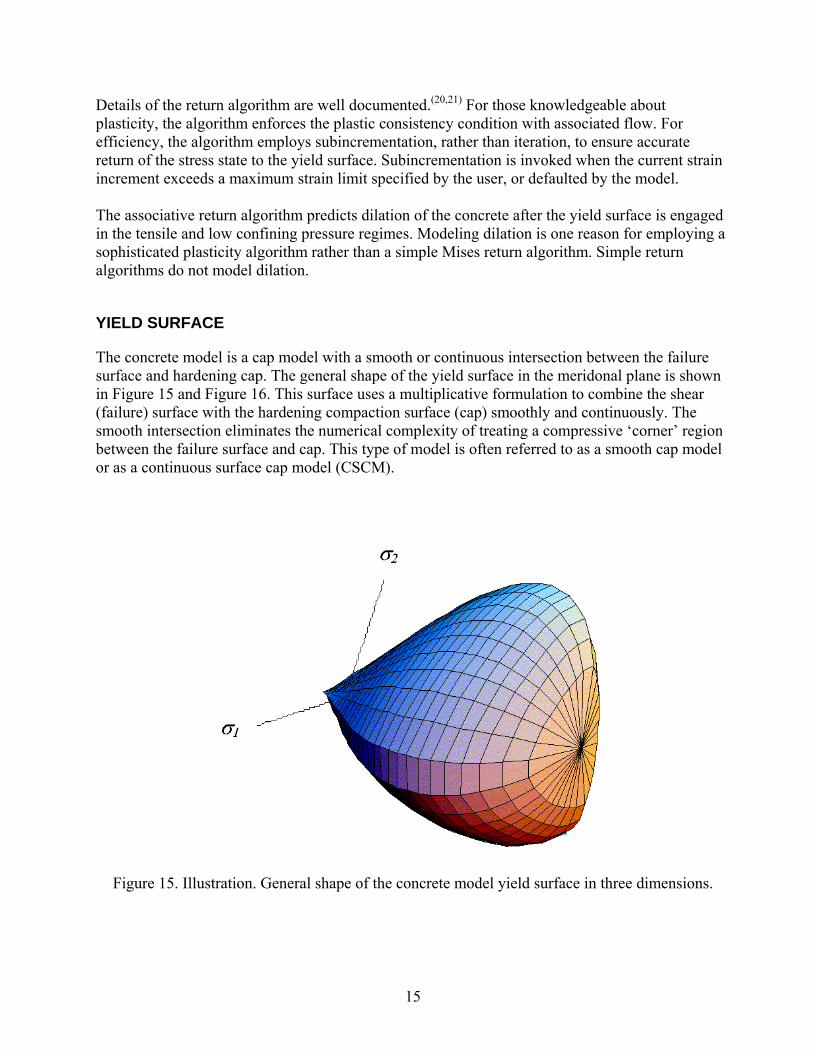
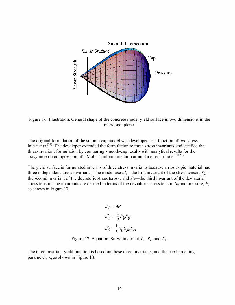
The concrete model is a cap model with a smooth or continuous intersection between the failure surface and hardening cap. The general shape of the yield surface in the meridonal plane is shown in Figure 15 and Figure 16. This surface uses a multiplicative formulation to combine the shear (failure) surface with the hardening compaction surface (cap) smoothly and continuously. The smooth intersection eliminates the numerical complexity of treating a compressive ‘corner’ region between the failure surface and cap. This type of model is often referred to as a smooth cap model or as a continuous surface cap model (CSCM).

Figure 15. Illustration. General shape of the concrete model yield surface in three dimensions.

16

Figure 16. Illustration. General shape of the concrete model yield surface in two dimensions in the meridonal plane.

The original formulation of the smooth cap model was developed as a function of two stress invariants.(22) The developer extended the formulation to three stress invariants and verified the three-invariant formulation by comparing smooth-cap results with analytical results for the axisymmetric compression of a Mohr-Coulomb medium around a circular hole.(20,23) The yield surface is formulated in terms of three stress invariants because an isotropic material has three independent stress invariants. The model uses J—the first invariant of the stress tensor, J′2—the second invariant of the deviatoric stress tensor, and J′3—the third invariant of the deviatoric stress tensor. The invariants are defined in terms of the deviatoric stress tensor, Sij and pressure, P, as shown in Figure 17:

Figure 17. Equation. Stress invariant J 1, J′2, and J′3.

The three invariant yield function is based on these three invariants, and the cap hardening parameter, κ, as shown in Figure 18:

17

Figure 18. Equation. Yield function f.

Here Ff is the shear failure surface, Fc is the hardening cap, and ℜ is the Rubin three-invariant reduction factor. Multiplying the cap ellipse function by the shear surface function allows the cap and shear surfaces to take on the same slope at their intersection, as discussed in subsequent paragraphs. Trial elastic stress invariants are temporarily updated via the trial elastic stress tensor, σT. These are denoted J1

T, J′2T, and J′3T. Elastic stress states are modeled when f (J1T, J′2T, J′3T, κΤ ) < 0.

Elastic-plastic stress states are modeled when f (J1T, J′2T, J′3T, κ Τ ) > 0. In this case, the plasticity

algorithm returns the stress state to the yield surface so that f (J1P, J′2P, J′3P, κ P) = 0.

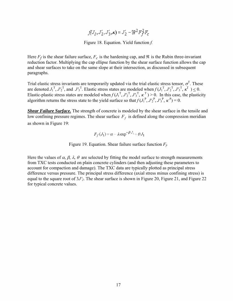
Shear Failure Surface. The strength of concrete is modeled by the shear surface in the tensile and low confining pressure regimes. The shear surface fF is defined along the compression meridian as shown in Figure 19:

Figure 19. Equation. Shear failure surface function Ff.

Here the values of α, β, λ, θ are selected by fitting the model surface to strength measurements from TXC tests conducted on plain concrete cylinders (and then adjusting these parameters to account for compaction and damage). The TXC data are typically plotted as principal stress difference versus pressure. The principal stress difference (axial stress minus confining stress) is equal to the square root of 3J′2. The shear surface is shown in Figure 20, Figure 21, and Figure 22 for typical concrete values.

18

psi = 145.05 MPa

Figure 20. Graph. Schematic of shear surface.

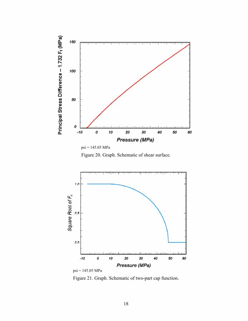
psi = 145.05 MPa Figure 21. Graph. Schematic of two-part cap function.

19

psi = 145.05 MPa

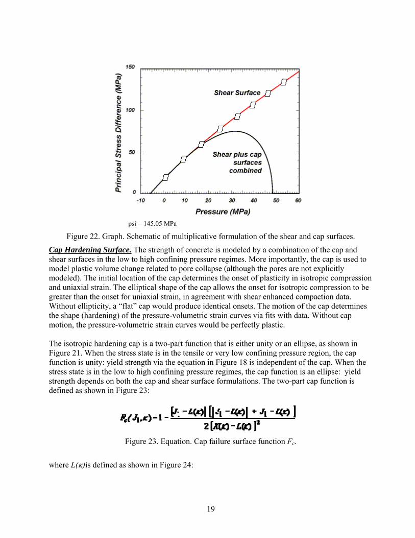
Figure 22. Graph. Schematic of multiplicative formulation of the shear and cap surfaces.

Cap Hardening Surface. The strength of concrete is modeled by a combination of the cap and shear surfaces in the low to high confining pressure regimes. More importantly, the cap is used to model plastic volume change related to pore collapse (although the pores are not explicitly modeled). The initial location of the cap determines the onset of plasticity in isotropic compression and uniaxial strain. The elliptical shape of the cap allows the onset for isotropic compression to be greater than the onset for uniaxial strain, in agreement with shear enhanced compaction data. Without ellipticity, a “flat” cap would produce identical onsets. The motion of the cap determines the shape (hardening) of the pressure-volumetric strain curves via fits with data. Without cap motion, the pressure-volumetric strain curves would be perfectly plastic. The isotropic hardening cap is a two-part function that is either unity or an ellipse, as shown in Figure 21. When the stress state is in the tensile or very low confining pressure region, the cap function is unity: yield strength via the equation in Figure 18 is independent of the cap. When the stress state is in the low to high confining pressure regimes, the cap function is an ellipse: yield strength depends on both the cap and shear surface formulations. The two-part cap function is defined as shown in Figure 23:

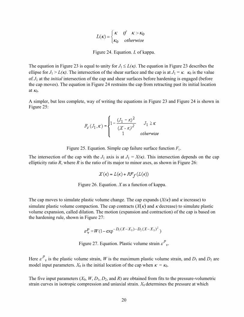
Figure 23. Equation. Cap failure surface function Fc.

where L(κ)is defined as shown in Figure 24:

20

Figure 24. Equation. L of kappa.

The equation in Figure 23 is equal to unity for J1 ≤ L(κ). The equation in Figure 23 describes the ellipse for J1 > L(κ). The intersection of the shear surface and the cap is at J1 = κ. κ0 is the value of J1 at the initial intersection of the cap and shear surfaces before hardening is engaged (before the cap moves). The equation in Figure 24 restrains the cap from retracting past its initial location at κ0. A simpler, but less complete, way of writing the equations in Figure 23 and Figure 24 is shown in Figure 25:

Figure 25. Equation. Simple cap failure surface function Fc.

The intersection of the cap with the J1 axis is at J1 = X(κ). This intersection depends on the cap ellipticity ratio R, where R is the ratio of its major to minor axes, as shown in Figure 26:

Figure 26. Equation. X as a function of kappa.

The cap moves to simulate plastic volume change. The cap expands (X(κ) and κ increase) to simulate plastic volume compaction. The cap contracts (X(κ) and κ decrease) to simulate plastic volume expansion, called dilation. The motion (expansion and contraction) of the cap is based on the hardening rule, shown in Figure 27:

Figure 27. Equation. Plastic volume strain ε pv.

Here ε p

v is the plastic volume strain, W is the maximum plastic volume strain, and D1 and D2 are model input parameters. X0 is the initial location of the cap when κ = κ0.

The five input parameters (X0, W, D1, D2, and R) are obtained from fits to the pressure-volumetric strain curves in isotropic compression and uniaxial strain. X0 determines the pressure at which

21

compaction initiates in isotropic compression. R, combined with X0, determines the pressure at which compaction initiates in uniaxial strain. D1 and D2 determine the shape of the pressure-volumetric strain curves. W determines the maximum plastic volume compaction.

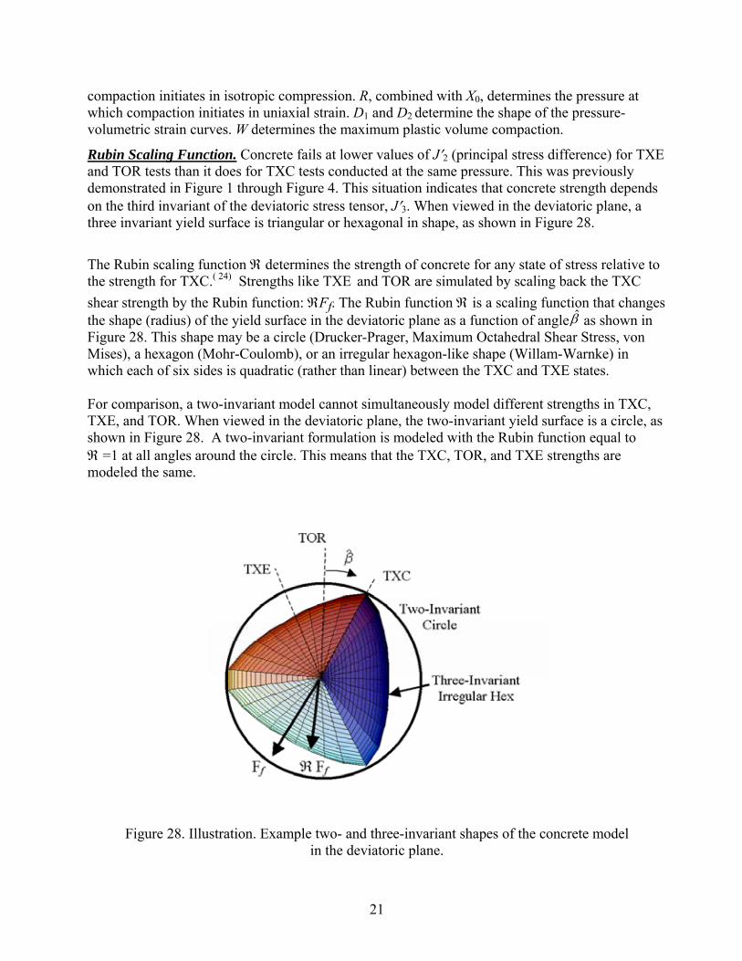
Rubin Scaling Function. Concrete fails at lower values of J′2 (principal stress difference) for TXE and TOR tests than it does for TXC tests conducted at the same pressure. This was previously demonstrated in Figure 1 through Figure 4. This situation indicates that concrete strength depends on the third invariant of the deviatoric stress tensor, J′3. When viewed in the deviatoric plane, a three invariant yield surface is triangular or hexagonal in shape, as shown in Figure 28.

The Rubin scaling function ℜ determines the strength of concrete for any state of stress relative to the strength for TXC.( 24) Strengths like TXE and TOR are simulated by scaling back the TXC shear strength by the Rubin function: ℜFf. The Rubin function ℜ is a scaling function that changes the shape (radius) of the yield surface in the deviatoric plane as a function of angle as shown in Figure 28. This shape may be a circle (Drucker-Prager, Maximum Octahedral Shear Stress, von Mises), a hexagon (Mohr-Coulomb), or an irregular hexagon-like shape (Willam-Warnke) in which each of six sides is quadratic (rather than linear) between the TXC and TXE states. For comparison, a two-invariant model cannot simultaneously model different strengths in TXC, TXE, and TOR. When viewed in the deviatoric plane, the two-invariant yield surface is a circle, as shown in Figure 28. A two-invariant formulation is modeled with the Rubin function equal to ℜ =1 at all angles around the circle. This means that the TXC, TOR, and TXE strengths are modeled the same.

Figure 28. Illustration. Example two- and three-invariant shapes of the concrete model in the deviatoric plane.

β̂

22

The angle is confined to the range -π/6 < < π and is related to the invariants J′2 and J′3, as shown in Figure 29:

Figure 29. Equation. Angle beta hat in the deviatoric plane.

I is a normalized invariant which remains in the range –1 < < 1. For the standard laboratory tests just discussed, the values of and are shown in Figure 30:

Figure 30. Equation. Relationship between beta hat and J hat.

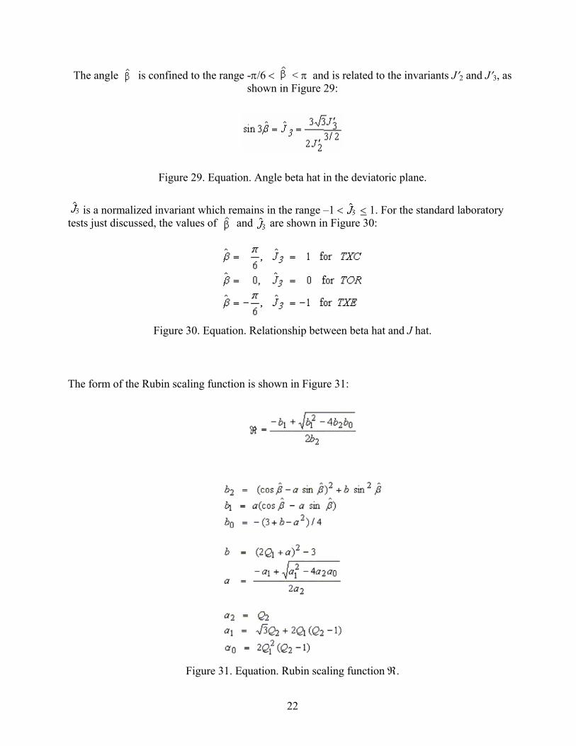
The form of the Rubin scaling function is shown in Figure 31:

Figure 31. Equation. Rubin scaling function ℜ.

23

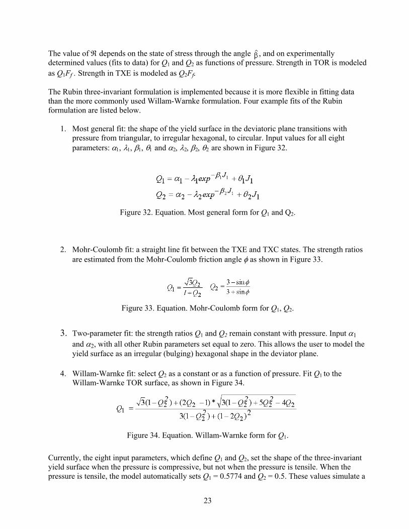
The value of ℜ depends on the state of stress through the angle , and on experimentally determined values (fits to data) for Q1 and Q2 as functions of pressure. Strength in TOR is modeled as Q1Ff . Strength in TXE is modeled as Q2Ff. The Rubin three-invariant formulation is implemented because it is more flexible in fitting data than the more commonly used Willam-Warnke formulation. Four example fits of the Rubin formulation are listed below.

1. Most general fit: the shape of the yield surface in the deviatoric plane transitions with pressure from triangular, to irregular hexagonal, to circular. Input values for all eight parameters: α1, λ1, β1, θ1 and α2, λ2, β2, θ2 are shown in Figure 32.

Figure 32. Equation. Most general form for Q1 and Q2.

2. Mohr-Coulomb fit: a straight line fit between the TXE and TXC states. The strength ratios

are estimated from the Mohr-Coulomb friction angle φ as shown in Figure 33.

Figure 33. Equation. Mohr-Coulomb form for Q1, Q2.

3. Two-parameter fit: the strength ratios Q1 and Q2 remain constant with pressure. Input α1

and α2, with all other Rubin parameters set equal to zero. This allows the user to model the yield surface as an irregular (bulging) hexagonal shape in the deviator plane.

4. Willam-Warnke fit: select Q2 as a constant or as a function of pressure. Fit Q1 to the

Willam-Warnke TOR surface, as shown in Figure 34.

Figure 34. Equation. Willam-Warnke form for Q1.

Currently, the eight input parameters, which define Q1 and Q2, set the shape of the three-invariant yield surface when the pressure is compressive, but not when the pressure is tensile. When the pressure is tensile, the model automatically sets Q1 = 0.5774 and Q2 = 0.5. These values simulate a

24

triangular yield surface in the deviatoric plane, and cannot be overridden by the user. With a triangular yield surface, the strengths attained in uniaxial, equal biaxial, and equal triaxial tensile stress simulations are approximately equal. For a smooth transition between the tensile and compressive pressure regions, the user should take care to set Q1 = 0.5774 and Q2 = 0.5 at zero pressure. This is accomplished by setting α1 – λ1 = 0.5774 and α2 – λ2 = 0.5774.

DAMAGE FORMULATION

Concrete exhibits softening (strength reduction) in the tensile and low to moderate compressive regimes. Softening is modeled via a damage formulation. Without the damage formulation, the cap model predicts perfectly plastic behavior for laboratory test simulations such as direct pull, unconfined compression, TXC, and TXE. This behavior is not realistic. Although perfectly plastic response is typical of concrete at high confining pressures, it is not representative of concrete at lower confinement and in tension.

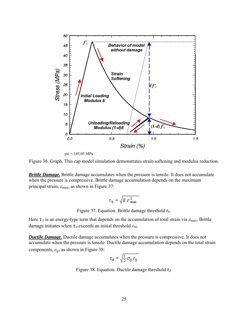
The damage formulation models both strain softening and modulus reduction. Strain softening is a decrease in strength during progressive straining after a peak strength value is reached. Modulus reduction is a decrease in the unloading/loading slopes typically observed in cyclic unload/load tests. The damage formulation is based on the work of Simo and Ju, shown in Figure 35.(25) Strain softening and modulus reduction are demonstrated in psi = 145.05 MPa Figure 36 for the concrete model.

Figure 35. Equation. Damaged stress σ dij.

Here d is a scalar damage parameter that transforms the stress tensor without damage, denoted σ vp, into the stress tensor with damage, denoted σ d. The damage formation is applied to the stresses after they are updated by the viscoplasticity algorithm. The damage parameter d ranges from zero for no damage to 1 for complete damage. Thus 1 − d is a reduction factor whose value depends on the accumulation of damage. The effect of this reduction factor is to reduce the bulk and shear moduli isotropically (simultaneously and proportionally). Damage initiates and accumulates when strain-based energy terms exceed the damage threshold. Damage accumulation via the parameter d is based on two distinct formulations, which is called brittle damage and ductile damage.

25

psi = 145.05 MPa

Figure 36. Graph. This cap model simulation demonstrates strain softening and modulus reduction.

Brittle Damage. Brittle damage accumulates when the pressure is tensile. It does not accumulate when the pressure is compressive. Brittle damage accumulation depends on the maximum principal strain, εmax, as shown in Figure 37:

Figure 37. Equation. Brittle damage threshold τb.

Here τ b is an energy-type term that depends on the accumulation of total strain via εmax. Brittle damage initiates when τ b exceeds an initial threshold r0b. Ductile Damage. Ductile damage accumulates when the pressure is compressive. It does not accumulate when the pressure is tensile. Ductile damage accumulation depends on the total strain components, εij, as shown in Figure 38:

Figure 38. Equation. Ductile damage threshold τd.

26

Here τd is an energy-type term. The stress components σij are the elasto-plastic stresses (with kinematic hardening) calculated before application of damage and rate effects. Therefore, this strain-energy term does not represent the true strain energy in the concrete. Ductile damage initiates when τ d exceeds an initial threshold r0d. Damage Threshold. Brittle and ductile damage initiate with plasticity. This effectively means that the initial damage surface is coincident with the plastic shear surface. Therefore, a distinct damage surface is not defined by the user. Damage initiates at peak strength on the shear surface where the plastic volume strain is dilative. Damage does not initiate on the cap where plastic volume strain is compactive. One exception to initiation of damage with initiation of plasticity is when rate effects are modeled via viscoplasticity. With viscoplasticity, the initial damage threshold is shifted (delayed), as shown in Figure 39:

Figure 39. Equation. Viscoplastic damage threshold r0.

Here r s is the damage threshold before application of viscoplasticity, and r0 is the shifted threshold

with viscoplasticity. When η is greater than zero (rate effects are modeled), the initial damage threshold is scaled up by the term in brackets. Hence, damage initiation is delayed while plasticity accumulates. This shift requires no input parameters and is hardwired into the model based on the viscoplastic theory previously discussed. Damage accumulates when either the brittle or ductile energy term, generically called τ n, exceeds the current damage threshold, rn. Here the subscript ‘n’ indicates the nth time step. Once damage initiates, the value of the damage threshold increases. The new threshold at time step n + 1, denoted rn+1, is set equal to the exceeded value of τ . If the previous value of τ did not exceed the previous threshold (an increment without damage), the threshold does not increase. Mathematically this is expressed as shown in Figure 40:

Figure 40. Equation. Incremental damage threshold, small rn+1.

Hence each strain energy term (brittle or ductile) must increase in value above its previous maximum in order for damage to accumulate. When energy remains constant or decreases, damage temporarily stops accumulating. The description given here is effectively that of an expanding damage surface.

27

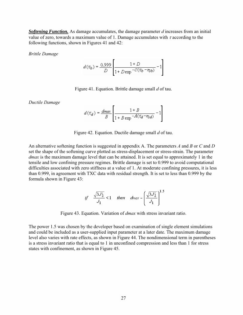
Softening Function. As damage accumulates, the damage parameter d increases from an initial value of zero, towards a maximum value of 1. Damage accumulates with τ according to the following functions, shown in Figures 41 and 42: Brittle Damage

Figure 41. Equation. Brittle damage small d of tau.

Ductile Damage

Figure 42. Equation. Ductile damage small d of tau.

An alternative softening function is suggested in appendix A. The parameters A and B or C and D set the shape of the softening curve plotted as stress-displacement or stress-strain. The parameter dmax is the maximum damage level that can be attained. It is set equal to approximately 1 in the tensile and low confining pressure regimes. Brittle damage is set to 0.999 to avoid computational difficulties associated with zero stiffness at a value of 1. At moderate confining pressures, it is less than 0.999, in agreement with TXC data with residual strength. It is set to less than 0.999 by the formula shown in Figure 43:

Figure 43. Equation. Variation of dmax with stress invariant ratio.

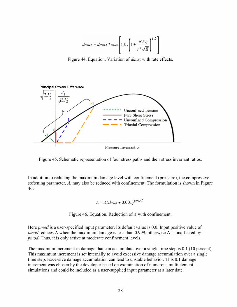
The power 1.5 was chosen by the developer based on examination of single element simulations and could be included as a user-supplied input parameter at a later date. The maximum damage level also varies with rate effects, as shown in Figure 44. The nondimensional term in parentheses is a stress invariant ratio that is equal to 1 in unconfined compression and less than 1 for stress states with confinement, as shown in Figure 45.

28

Figure 44. Equation. Variation of dmax with rate effects.

Figure 45. Schematic representation of four stress paths and their stress invariant ratios.

In addition to reducing the maximum damage level with confinement (pressure), the compressive softening parameter, A, may also be reduced with confinement. The formulation is shown in Figure 46:

Figure 46. Equation. Reduction of A with confinement.

Here pmod is a user-specified input parameter. Its default value is 0.0. Input positive value of pmod reduces A when the maximum damage is less than 0.999; otherwise A is unaffected by pmod. Thus, it is only active at moderate confinement levels. The maximum increment in damage that can accumulate over a single time step is 0.1 (10 percent). This maximum increment is set internally to avoid excessive damage accumulation over a single time step. Excessive damage accumulation can lead to unstable behavior. This 0.1 damage increment was chosen by the developer based on examination of numerous multielement simulations and could be included as a user-supplied input parameter at a later date.

29

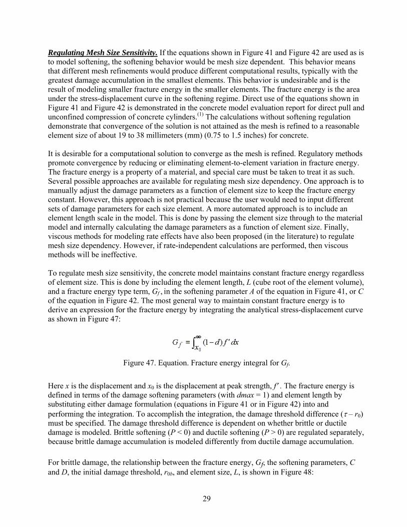
Regulating Mesh Size Sensitivity. If the equations shown in Figure 41 and Figure 42 are used as is to model softening, the softening behavior would be mesh size dependent. This behavior means that different mesh refinements would produce different computational results, typically with the greatest damage accumulation in the smallest elements. This behavior is undesirable and is the result of modeling smaller fracture energy in the smaller elements. The fracture energy is the area under the stress-displacement curve in the softening regime. Direct use of the equations shown in Figure 41 and Figure 42 is demonstrated in the concrete model evaluation report for direct pull and unconfined compression of concrete cylinders.(1) The calculations without softening regulation demonstrate that convergence of the solution is not attained as the mesh is refined to a reasonable element size of about 19 to 38 millimeters (mm) (0.75 to 1.5 inches) for concrete. It is desirable for a computational solution to converge as the mesh is refined. Regulatory methods promote convergence by reducing or eliminating element-to-element variation in fracture energy. The fracture energy is a property of a material, and special care must be taken to treat it as such. Several possible approaches are available for regulating mesh size dependency. One approach is to manually adjust the damage parameters as a function of element size to keep the fracture energy constant. However, this approach is not practical because the user would need to input different sets of damage parameters for each size element. A more automated approach is to include an element length scale in the model. This is done by passing the element size through to the material model and internally calculating the damage parameters as a function of element size. Finally, viscous methods for modeling rate effects have also been proposed (in the literature) to regulate mesh size dependency. However, if rate-independent calculations are performed, then viscous methods will be ineffective. To regulate mesh size sensitivity, the concrete model maintains constant fracture energy regardless of element size. This is done by including the element length, L (cube root of the element volume), and a fracture energy type term, Gf , in the softening parameter A of the equation in Figure 41, or C of the equation in Figure 42. The most general way to maintain constant fracture energy is to derive an expression for the fracture energy by integrating the analytical stress-displacement curve as shown in Figure 47:

Figure 47. Equation. Fracture energy integral for Gf.

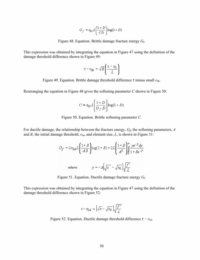
Here x is the displacement and x0 is the displacement at peak strength, f′ . The fracture energy is defined in terms of the damage softening parameters (with dmax = 1) and element length by substituting either damage formulation (equations in Figure 41 or in Figure 42) into and performing the integration. To accomplish the integration, the damage threshold difference (τ – r0) must be specified. The damage threshold difference is dependent on whether brittle or ductile damage is modeled. Brittle softening (P < 0) and ductile softening (P > 0) are regulated separately, because brittle damage accumulation is modeled differently from ductile damage accumulation. For brittle damage, the relationship between the fracture energy, Gf, the softening parameters, C and D, the initial damage threshold, r0b, and element size, L, is shown in Figure 48:

30

Figure 48. Equation. Brittle damage fracture energy Gf.

This expression was obtained by integrating the equation in Figure 47 using the definition of the damage threshold difference shown in Figure 49:

Figure 49. Equation. Brittle damage threshold difference τ minus small r0b.

Rearranging the equation in Figure 48 gives the softening parameter C shown in Figure 50:

Figure 50. Equation. Brittle softening parameter C.

For ductile damage, the relationship between the fracture energy, Gf, the softening parameters, A and B, the initial damage threshold, r0d, and element size, L, is shown in Figure 51:

Figure 51. Equation. Ductile damage fracture energy Gf.

This expression was obtained by integrating the equation in Figure 47 using the definition of the damage threshold difference shown in Figure 52:

Figure 52. Equation. Ductile damage threshold difference τ − r0d.

31

The integral on the right of the equation in Figure 51 reduces to a dilogarithm, which is not solvable in closed form. Therefore, its value is internally calculated by the LS-DYNA concrete model during the initialization phase. Its value depends on the input parameter B and is termed dilog. Rearranging the equation in Figure 51 gives the softening parameter A shown in Figure 53:

Figure 53. Equation. Ductile softening parameter A.

In summary, to regulate mesh size dependency, the concrete model requires input values for B and Gfc rather than for A and B. Similarly, the concrete model requires input values for D and Gft rather than for C and D. When the brittle damage threshold is attained, the concrete material model internally solves the equation in Figure 48 for the value of A based on the initial element size, the initial brittle damage threshold, the brittle fracture energy, and a user-specified input value for B. When the ductile damage threshold is attained, the concrete material model internally solves the equation in Figure 51 for the value of C based on the initial element size, the initial ductile damage threshold, and the ductile fracture energy, and a user-specified input value for D. Refer to the concrete model evaluation report, which discusses cylinder compression calculations conducted with regulation of the softening response.(1) The calculations conducted in tension demonstrate that brittleness increases with mesh refinement until convergence is attained. Conversely, the calculations conducted in compression demonstrate that brittleness decreases with mesh refinement until convergence is attained. Specifying the Fracture Energy. The user specifies three distinct fracture energy values. These are the fracture energy in uniaxial tensile stress, Gft, pure shear stress, Gfs, and uniaxial compressive stress, Gfc. The model internally selects the brittle or ductile fracture energy from equations that interpolate between the three fracture energy values as a function of the stress state. The stress state is defined by a nondimensional stress invariant ratio call trans. The interpolation is as shown in Figures 54 and 55:

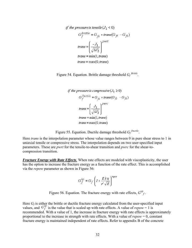
32

Figure 54. Equation. Brittle damage threshold Gf Brittle.

Figure 55. Equation. Ductile damage threshold Gf

Ductile.

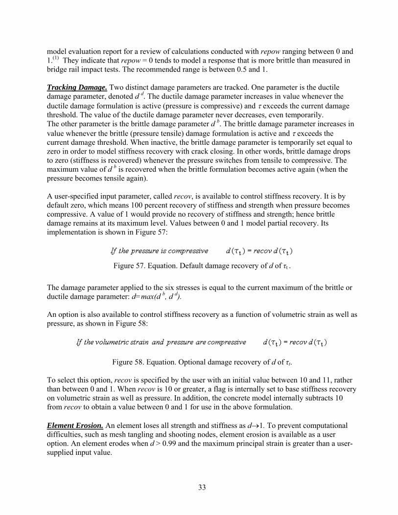
Here trans is the interpolation parameter whose value ranges between 0 in pure shear stress to 1 in uniaxial tensile or compressive stress. The interpolation depends on two user-specified input parameters. These are pwrt for the tensile-to-shear transition and pwrc for the shear-to-compression transition. Fracture Energy with Rate Effects. When rate effects are modeled with viscoplasticity, the user has the option to increase the fracture energy as a function of the rate effect. This is accomplished via the repow parameter as shown in Figure 56:

Figure 56. Equation. The fracture energy with rate effects, Gvp

f .

Here Gf is either the brittle or ductile fracture energy calculated from the user-specified input values, and is the value that is scaled up with rate effects. A value of repow = 1 is recommended. With a value of 1, the increase in fracture energy with rate effects is approximately proportional to the increase in strength with rate effects. With a value of repow = 0, constant fracture energy is maintained independent of rate effects. Refer to appendix B of the concrete

vp f G

33

model evaluation report for a review of calculations conducted with repow ranging between 0 and 1.(1) They indicate that repow = 0 tends to model a response that is more brittle than measured in bridge rail impact tests. The recommended range is between 0.5 and 1. Tracking Damage. Two distinct damage parameters are tracked. One parameter is the ductile damage parameter, denoted d d. The ductile damage parameter increases in value whenever the ductile damage formulation is active (pressure is compressive) and τ exceeds the current damage threshold. The value of the ductile damage parameter never decreases, even temporarily. The other parameter is the brittle damage parameter d b. The brittle damage parameter increases in value whenever the brittle (pressure tensile) damage formulation is active and τ exceeds the current damage threshold. When inactive, the brittle damage parameter is temporarily set equal to zero in order to model stiffness recovery with crack closing. In other words, brittle damage drops to zero (stiffness is recovered) whenever the pressure switches from tensile to compressive. The maximum value of d b is recovered when the brittle formulation becomes active again (when the pressure becomes tensile again). A user-specified input parameter, called recov, is available to control stiffness recovery. It is by default zero, which means 100 percent recovery of stiffness and strength when pressure becomes compressive. A value of 1 would provide no recovery of stiffness and strength; hence brittle damage remains at its maximum level. Values between 0 and 1 model partial recovery. Its implementation is shown in Figure 57:

Figure 57. Equation. Default damage recovery of d of τt .

The damage parameter applied to the six stresses is equal to the current maximum of the brittle or ductile damage parameter: d=max(d b, d d). An option is also available to control stiffness recovery as a function of volumetric strain as well as pressure, as shown in Figure 58:

Figure 58. Equation. Optional damage recovery of d of τt. To select this option, recov is specified by the user with an initial value between 10 and 11, rather than between 0 and 1. When recov is 10 or greater, a flag is internally set to base stiffness recovery on volumetric strain as well as pressure. In addition, the concrete model internally subtracts 10 from recov to obtain a value between 0 and 1 for use in the above formulation. Element Erosion. An element loses all strength and stiffness as d→1. To prevent computational difficulties, such as mesh tangling and shooting nodes, element erosion is available as a user option. An element erodes when d > 0.99 and the maximum principal strain is greater than a user-supplied input value.

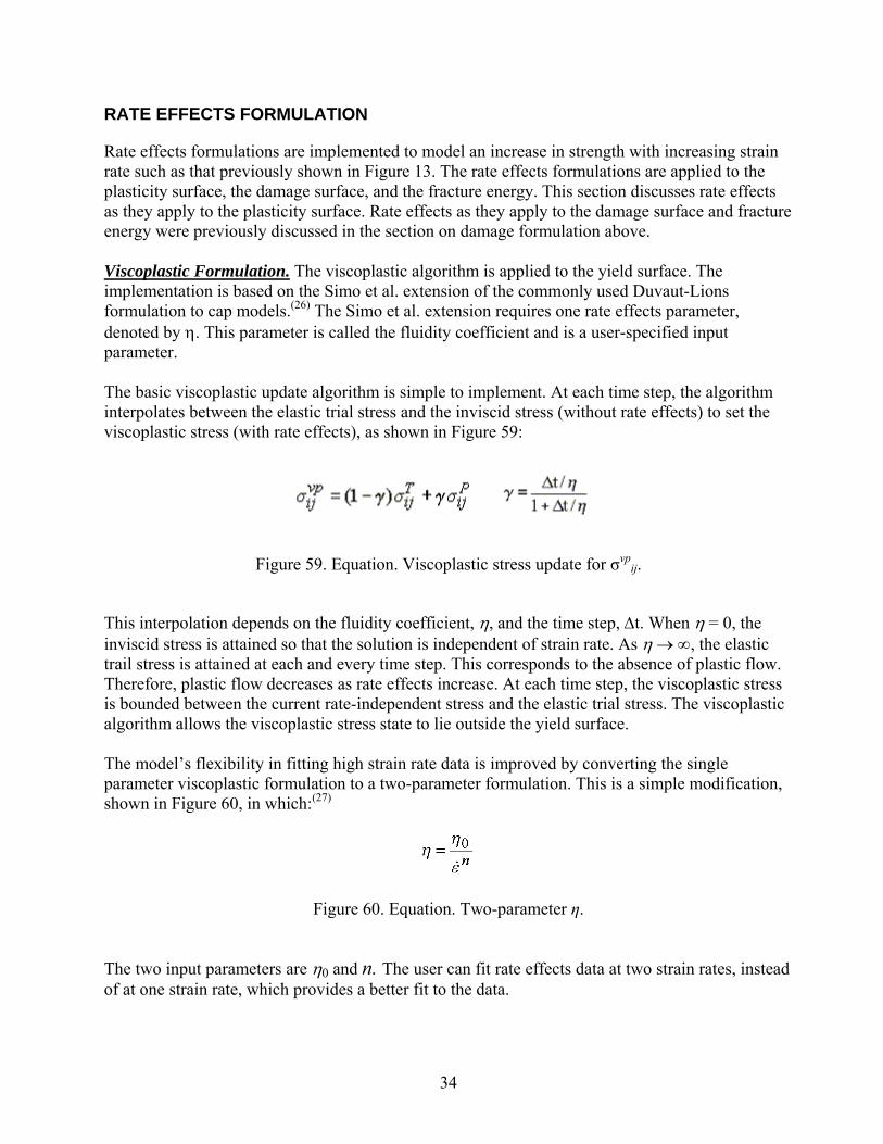
34

RATE EFFECTS FORMULATION

Rate effects formulations are implemented to model an increase in strength with increasing strain rate such as that previously shown in Figure 13. The rate effects formulations are applied to the plasticity surface, the damage surface, and the fracture energy. This section discusses rate effects as they apply to the plasticity surface. Rate effects as they apply to the damage surface and fracture energy were previously discussed in the section on damage formulation above. Viscoplastic Formulation. The viscoplastic algorithm is applied to the yield surface. The implementation is based on the Simo et al. extension of the commonly used Duvaut-Lions formulation to cap models.(26) The Simo et al. extension requires one rate effects parameter, denoted by η. This parameter is called the fluidity coefficient and is a user-specified input parameter. The basic viscoplastic update algorithm is simple to implement. At each time step, the algorithm interpolates between the elastic trial stress and the inviscid stress (without rate effects) to set the viscoplastic stress (with rate effects), as shown in Figure 59:

Figure 59. Equation. Viscoplastic stress update for σvpij.

This interpolation depends on the fluidity coefficient, η, and the time step, Δt. When η = 0, the inviscid stress is attained so that the solution is independent of strain rate. As η → ∞, the elastic trail stress is attained at each and every time step. This corresponds to the absence of plastic flow. Therefore, plastic flow decreases as rate effects increase. At each time step, the viscoplastic stress is bounded between the current rate-independent stress and the elastic trial stress. The viscoplastic algorithm allows the viscoplastic stress state to lie outside the yield surface. The model’s flexibility in fitting high strain rate data is improved by converting the single parameter viscoplastic formulation to a two-parameter formulation. This is a simple modification, shown in Figure 60, in which:(27)

Figure 60. Equation. Two-parameter η.

The two input parameters are η0 and n. The user can fit rate effects data at two strain rates, instead of at one strain rate, which provides a better fit to the data.

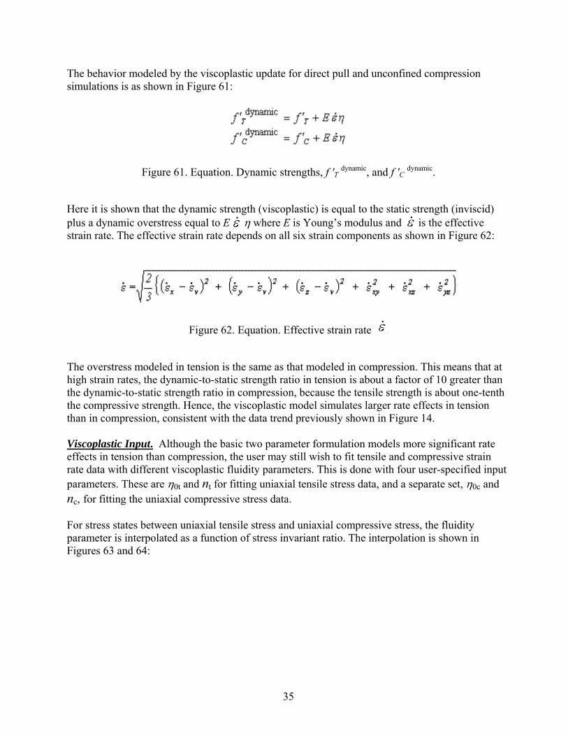
35

The behavior modeled by the viscoplastic update for direct pull and unconfined compression simulations is as shown in Figure 61:

Figure 61. Equation. Dynamic strengths, f ′T dynamic, and f ′C dynamic.

Here it is shown that the dynamic strength (viscoplastic) is equal to the static strength (inviscid) plus a dynamic overstress equal to E η where E is Young’s modulus and is the effective strain rate. The effective strain rate depends on all six strain components as shown in Figure 62:

Figure 62. Equation. Effective strain rate .

The overstress modeled in tension is the same as that modeled in compression. This means that at high strain rates, the dynamic-to-static strength ratio in tension is about a factor of 10 greater than the dynamic-to-static strength ratio in compression, because the tensile strength is about one-tenth the compressive strength. Hence, the viscoplastic model simulates larger rate effects in tension than in compression, consistent with the data trend previously shown in Figure 14. Viscoplastic Input. Although the basic two parameter formulation models more significant rate effects in tension than compression, the user may still wish to fit tensile and compressive strain rate data with different viscoplastic fluidity parameters. This is done with four user-specified input parameters. These are η0t and nt for fitting uniaxial tensile stress data, and a separate set, η0c and nc, for fitting the uniaxial compressive stress data. For stress states between uniaxial tensile stress and uniaxial compressive stress, the fluidity parameter is interpolated as a function of stress invariant ratio. The interpolation is shown in Figures 63 and 64:

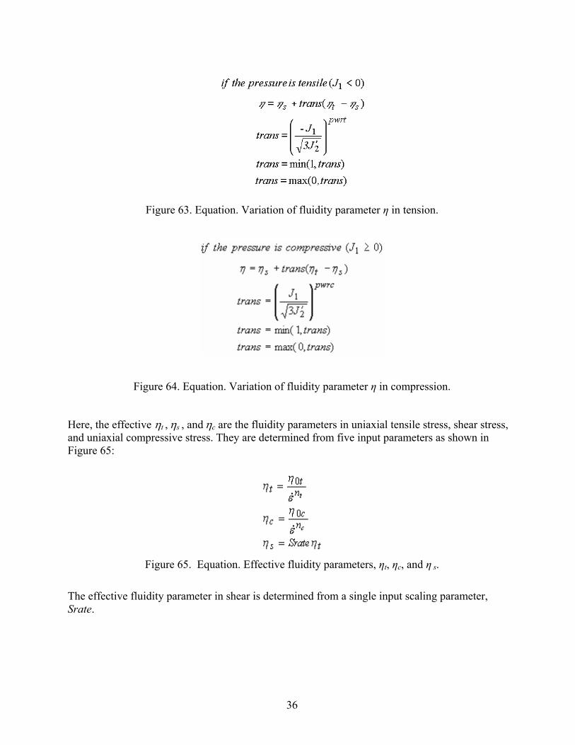
36

Figure 63. Equation. Variation of fluidity parameter η in tension.

Figure 64. Equation. Variation of fluidity parameter η in compression.

Here, the effective ηt , ηs , and ηc are the fluidity parameters in uniaxial tensile stress, shear stress, and uniaxial compressive stress. They are determined from five input parameters as shown in Figure 65:

Figure 65. Equation. Effective fluidity parameters, ηt, ηc, and η s.

The effective fluidity parameter in shear is determined from a single input scaling parameter, Srate.

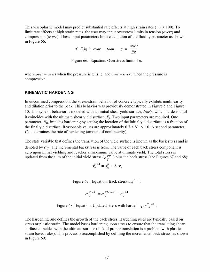
37

This viscoplastic model may predict substantial rate effects at high strain rates ( > 100). To limit rate effects at high strain rates, the user may input overstress limits in tension (overt) and compression (overc). These input parameters limit calculation of the fluidity parameter as shown in Figure 66:

Figure 66. Equation. Overstress limit of η.

where over = overt when the pressure is tensile, and over = overc when the pressure is compressive.

KINEMATIC HARDENING

In unconfined compression, the stress-strain behavior of concrete typically exhibits nonlinearity and dilation prior to the peak. This behavior was previously demonstrated in Figure 5 and Figure 10. This type of behavior is modeled with an initial shear yield surface, NHFf , which hardens until it coincides with the ultimate shear yield surface, Ff. Two input parameters are required. One parameter, NH, initiates hardening by setting the location of the initial yield surface as a fraction of the final yield surface. Reasonable values are approximately 0.7 < NH ≤ 1.0. A second parameter, CH, determines the rate of hardening (amount of nonlinearity). The state variable that defines the translation of the yield surface is known as the back stress and is denoted by αij. The incremental backstress is Δαij. The value of each back stress component is zero upon initial yielding and reaches a maximum value at ultimate yield. The total stress is updated from the sum of the initial yield stress ( ) plus the back stress (see Figures 67 and 68):

Figure 67. Equation. Back stress α ij n + 1.

Figure 68. Equation. Updated stress with hardening, σP

ij n+1.

The hardening rule defines the growth of the back stress. Hardening rules are typically based on stress or plastic strain. The model bases hardening upon stress to ensure that the translating shear surface coincides with the ultimate surface (lack of proper translation is a problem with plastic strain based rules). This process is accomplished by defining the incremental back stress, as shown in Figure 69:

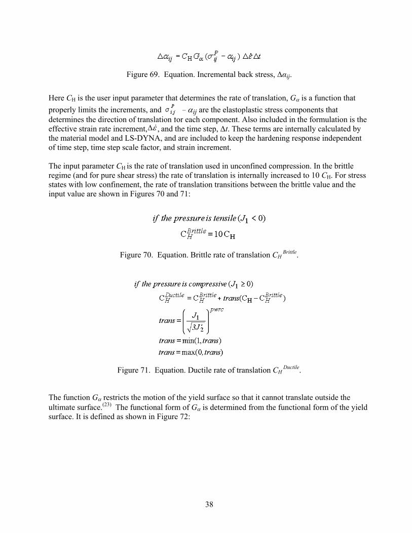
38

Figure 69. Equation. Incremental back stress, Δαij.

Here CH is the user input parameter that determines the rate of translation, Gα is a function that properly limits the increments, and – αij are the elastoplastic stress components that determines the direction of translation for each component. Also included in the formulation is the effective strain rate increment, , and the time step, Δt. These terms are internally calculated by the material model and LS-DYNA, and are included to keep the hardening response independent of time step, time step scale factor, and strain increment. The input parameter CH is the rate of translation used in unconfined compression. In the brittle regime (and for pure shear stress) the rate of translation is internally increased to 10 CH. For stress states with low confinement, the rate of translation transitions between the brittle value and the input value are shown in Figures 70 and 71:

Figure 70. Equation. Brittle rate of translation CH

Brittle.

Figure 71. Equation. Ductile rate of translation CH

Ductile.

The function Gα restricts the motion of the yield surface so that it cannot translate outside the ultimate surface.(23) The functional form of Gα is determined from the functional form of the yield surface. It is defined as shown in Figure 72:

ε&Δ

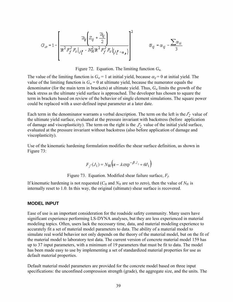
39

2J ′

2J ′

Figure 72. Equation. The limiting function Gα.

The value of the limiting function is Gα = 1 at initial yield, because αij = 0 at initial yield. The value of the limiting function is Gα = 0 at ultimate yield, because the numerator equals the denominator (for the main term in brackets) at ultimate yield. Thus, Gα limits the growth of the back stress as the ultimate yield surface is approached. The developer has chosen to square the term in brackets based on review of the behavior of single element simulations. The square power could be replaced with a user-defined input parameter at a later date. Each term in the denominator warrants a verbal description. The term on the left is the value of the ultimate yield surface, evaluated at the pressure invariant with backstress (before application of damage and viscoplasticity). The term on the right is the value of the initial yield surface, evaluated at the pressure invariant without backstress (also before application of damage and viscoplasticity). Use of the kinematic hardening formulation modifies the shear surface definition, as shown in Figure 73:

Figure 73. Equation. Modified shear failure surface, Ff.

If kinematic hardening is not requested (CH and NH are set to zero), then the value of NH is internally reset to 1.0. In this way, the original (ultimate) shear surface is recovered.

MODEL INPUT

Ease of use is an important consideration for the roadside safety community. Many users have significant experience performing LS-DYNA analyses, but they are less experienced in material modeling topics. Often, users lack the necessary time, data, and material modeling experience to accurately fit a set of material model parameters to data. The ability of a material model to simulate real world behavior not only depends on the theory of the material model, but on the fit of the material model to laboratory test data. The current version of concrete material model 159 has up to 37 input parameters, with a minimum of 19 parameters that must be fit to data. The model has been made easy to use by implementing a set of standardized material properties for use as default material properties. Default material model parameters are provided for the concrete model based on three input specifications: the unconfined compression strength (grade), the aggregate size, and the units. The

40

parameters are fit to data for unconfined compression strengths between about 20 and 58 MPa (2,901 to 8,412 psi), with emphasis on the midrange between 28 and 48 MPa (4,061 and 6,962 psi). The unconfined compression strength affects all aspects of the fit, including stiffness, three-dimensional yield strength, hardening, and damage. The fracture energy affects only the softening behavior of the damage formulation. Softening is fit to data for aggregate sizes between 8 and 32 mm (0.3 and 1.3 inches). The suite of material properties was primarily obtained through use of the CEB-FIP Model Code.(11) This code is a synthesis of research findings and contains a thorough section on concrete classification and constitutive relations. Various material properties, such as compressive and tensile strengths, stiffness, and fracture energy, are reported as a function of grade and aggregate size.

Bulk and Shear Moduli

Young’s modulus of concrete varies with concrete strength, as shown in Table 1. These measurements are taken from an equation in CEB, as shown in Figure 74:

Figure 74. Equation. Default Young’s modulus E.

Here, E is Young’s modulus and EC = 18.275 MPa (2,651 psi) (which is the value of Young’s modulus when f ' c = 10 MPa (1,450 psi)). This value of EC is for simulations that are modeled linear to the peak (no prepeak hardening). Poisson’s ratio is typically taken as being between 0.1 and 0.2. A value of ν = 0.15 is selected here and is assumed to remain constant with concrete strength. Based on this information, the default bulk and shear moduli (K and G) in Table 1 are derived from the classical relationships between stiffness constants, as shown in Figure 75:

Figure 75. Equation. Shear and bulk moduli, G and K.

The equations in Figure 74 and Figure 75 are implemented in the concrete model initialization routines to set the default moduli of concrete as a function of concrete compressive strength. Alternatively, the ACI Committee 318 suggests the formula shown in Figure 76 for the elastic modulus:

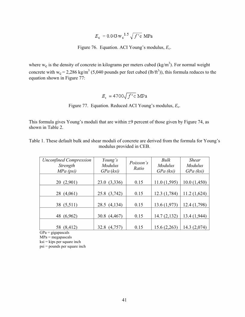
41

Figure 76. Equation. ACI Young’s modulus, Ec.

where wc is the density of concrete in kilograms per meters cubed (kg/m3). For normal weight concrete with wc = 2,286 kg/m3 (5,040 pounds per feet cubed (lb/ft3)), this formula reduces to the equation shown in Figure 77:

Figure 77. Equation. Reduced ACI Young’s modulus, Ec.

This formula gives Young’s moduli that are within ±9 percent of those given by Figure 74, as shown in Table 2.

Table 1. These default bulk and shear moduli of concrete are derived from the formula for Young’s modulus provided in CEB.

Unconfined Compression

Strength MPa (psi)

Young’s Modulus GPa (ksi)

Poisson’s Ratio

Bulk Modulus GPa (ksi)

Shear Modulus GPa (ksi)

20 (2,901)

23.0 (3,336)

0.15

11.0 (1,595)

10.0 (1,450)

28 (4,061)

25.8 (3,742)

0.15

12.3 (1,784)

11.2 (1,624)

38 (5,511)

28.5 (4,134)

0.15

13.6 (1,973)

12.4 (1,798)

48 (6,962)

30.8 (4,467)

0.15

14.7 (2,132)

13.4 (1,944)

58 (8,412)

32.8 (4,757)

0.15

15.6 (2,263)

14.3 (2,074)

GPa = gigapascals MPa = megapascals ksi = kips per square inch psi = pounds per square inch

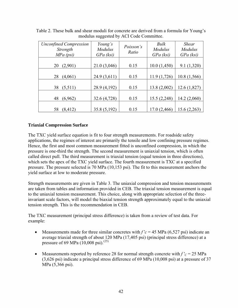
42

Table 2. These bulk and shear moduli for concrete are derived from a formula for Young’s modulus suggested by ACI Code Committee.

Unconfined Compression Strength

MPa (psi)

Young’s Modulus GPa (ksi)

Poisson’s Ratio

Bulk Modulus GPa (ksi)

Shear Modulus GPa (ksi)

20 (2,901)

21.0 (3,046)

0.15

10.0 (1,450)

9.1 (1,320)

28 (4,061)

24.9 (3,611)

0.15

11.9 (1,726)

10.8 (1,566)

38 (5,511)

28.9 (4,192)

0.15

13.8 (2,002)

12.6 (1,827)

48 (6,962)

32.6 (4,728)

0.15

15.5 (2,248)

14.2 (2,060)

58 (8,412)

35.8 (5,192)

0.15

17.0 (2,466)

15.6 (2,263)

Triaxial Compression Surface

The TXC yield surface equation is fit to four strength measurements. For roadside safety applications, the regimes of interest are primarily the tensile and low confining pressure regimes. Hence, the first and most common measurement fitted is unconfined compression, in which the pressure is one-third the strength. The second measurement is uniaxial tension, which is often called direct pull. The third measurement is triaxial tension (equal tension in three directions), which sets the apex of the TXC yield surface. The fourth measurement is TXC at a specified pressure. The pressure selected is 70 MPa (10,153 psi). The fit to this measurement anchors the yield surface at low to moderate pressure. Strength measurements are given in Table 3. The uniaxial compression and tension measurements are taken from tables and information provided in CEB. The triaxial tension measurement is equal to the uniaxial tension measurement. This choice, along with appropriate selection of the three-invariant scale factors, will model the biaxial tension strength approximately equal to the uniaxial tension strength. This is the recommendation in CEB. The TXC measurement (principal stress difference) is taken from a review of test data. For example:

• Measurements made for three similar concretes with f 'c = 45 MPa (6,527 psi) indicate an average triaxial strength of about 120 MPa (17,405 psi) (principal stress difference) at a pressure of 69 MPa (10,008 psi).(25)

• Measurements reported by reference 28 for normal strength concrete with f 'C = 25 MPa (3,626 psi) indicate a principal stress difference of 69 MPa (10,008 psi) at a pressure of 37 MPa (5,366 psi).

43

Table 3. Approximate strength measurements used to set default TXC yield surface parameters.

Measurement Type

Strengths Set 1

Strengths

Set 2

Strengths

Set 3

Strengths

Set 4

Strengths

Set 5 Uniaxial Compression f 'C MPa (psi)

20 (2,901)

28 (4,061)

38 (5,511)

48 (6,962)

58 (8,412)

Uniaxial Tension f 'T MPa (psi)

1.6 (232)

2.2 (319.1)

2.9 (421)

3.5 (508)

4.1 (595)

Triaxial Tension MPa (psi)

1.6 (232)

2.2 (319.1)

2.9 (421)

3.5 (508)

4.1 (595)

Triaxial Compression 2.75 f 'C at P = 1.5 f 'C MPa (psi)

55 (7,977)

77 (11,168)

105 (15,229)

132 (19,145)

160 (23,206)

The TXC yield surface equation relates strength to pressure via four parameters as shown in Figure 78:

Figure 78. Equation. TXC Strength.

At each value of unconfined compressive strength, the four strength parameters (α, λ, β, θ ) are simultaneously fit to the four strength values via an iterative procedure. Fitted values at five strengths are given in Table 4. Obviously, a user may wish to analyze concrete at strengths other than the five listed. To accomplish this, quadratic equations as a function of unconfined compression strength are fit through each parameter, P, as shown in Figure 79:

Figure 79. Equation. Interpolation parameter P.

For the TXC yield surface, the parameter P represents either α, λ, β, or θ. The fitted values of AP, BP, and CP are given in Table 5. Fitted values of AP, BP, and CP for all other concrete model input parameters (TOR and TXE yield surfaces, cap, damage, rate effects parameters) are given in subsequent sections.

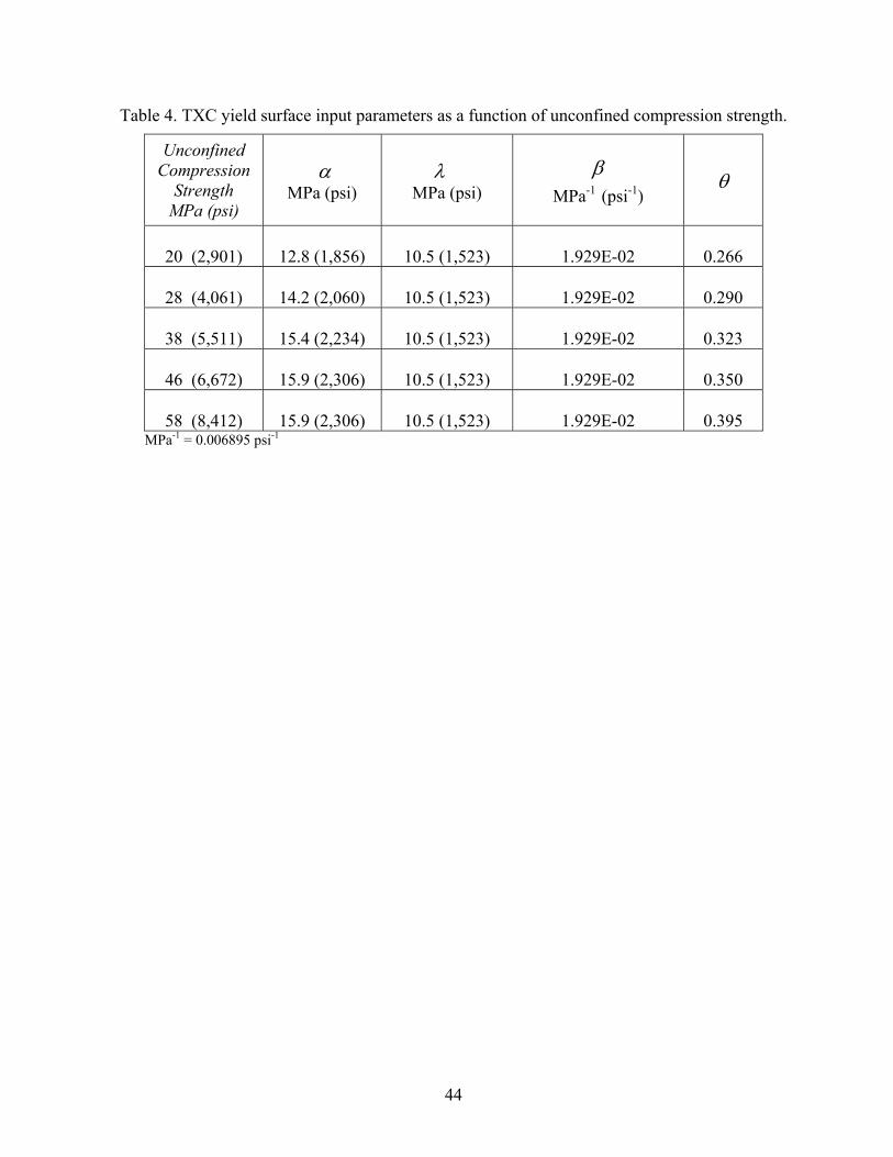
44

Table 4. TXC yield surface input parameters as a function of unconfined compression strength.

Unconfined Compression

Strength MPa (psi)

α MPa (psi)

λ MPa (psi)

β

MPa-1 (psi-1) θ

20 (2,901)

12.8 (1,856)

10.5 (1,523)

1.929E-02

0.266

28 (4,061)

14.2 (2,060)

10.5 (1,523)

1.929E-02

0.290

38 (5,511)

15.4 (2,234)

10.5 (1,523)

1.929E-02

0.323

46 (6,672)

15.9 (2,306)

10.5 (1,523)

1.929E-02

0.350

58 (8,412)

15.9 (2,306)

10.5 (1,523)

1.929E-02

0.395

MPa-1 = 0.006895 psi-1

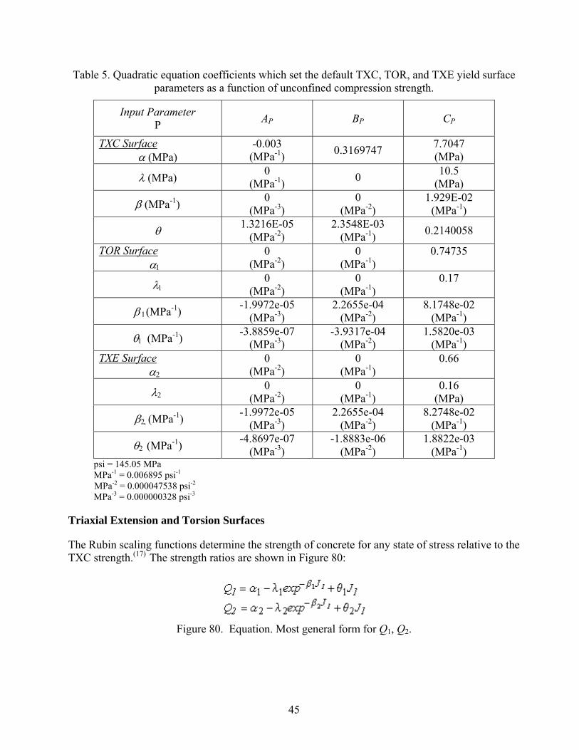
45

Table 5. Quadratic equation coefficients which set the default TXC, TOR, and TXE yield surface parameters as a function of unconfined compression strength.

Input Parameter P AP BP CP

TXC Surface α (MPa)

-0.003 (MPa-1) 0.3169747 7.7047

(MPa)

λ (MPa) 0 (MPa-1) 0 10.5

(MPa)

β (MPa-1) 0 (MPa-3)

0 (MPa-2)

1.929E-02 (MPa-1)

θ 1.3216E-05 (MPa-2)

2.3548E-03 (MPa-1) 0.2140058

TOR Surface α1

0 (MPa-2)

0 (MPa-1)

0.74735

λ1 0 (MPa-2)

0 (MPa-1)

0.17

β 1(MPa-1) -1.9972e-05 (MPa-3)

2.2655e-04 (MPa-2)

8.1748e-02 (MPa-1)

θ1 (MPa-1) -3.8859e-07 (MPa-3)

-3.9317e-04 (MPa-2)

1.5820e-03 (MPa-1)

TXE Surface α2

0 (MPa-2)

0 (MPa-1)

0.66

λ2 0 (MPa-2)

0 (MPa-1)

0.16 (MPa)

β2 (MPa-1) -1.9972e-05 (MPa-3)

2.2655e-04 (MPa-2)

8.2748e-02 (MPa-1)

θ2 (MPa-1) -4.8697e-07 (MPa-3)

-1.8883e-06 (MPa-2)

1.8822e-03 (MPa-1)

psi = 145.05 MPa MPa-1 = 0.006895 psi-1

MPa-2 = 0.000047538 psi-2 MPa-3 = 0.000000328 psi-3

Triaxial Extension and Torsion Surfaces

The Rubin scaling functions determine the strength of concrete for any state of stress relative to the TXC strength.(17) The strength ratios are shown in Figure 80:

Figure 80. Equation. Most general form for Q1, Q2.

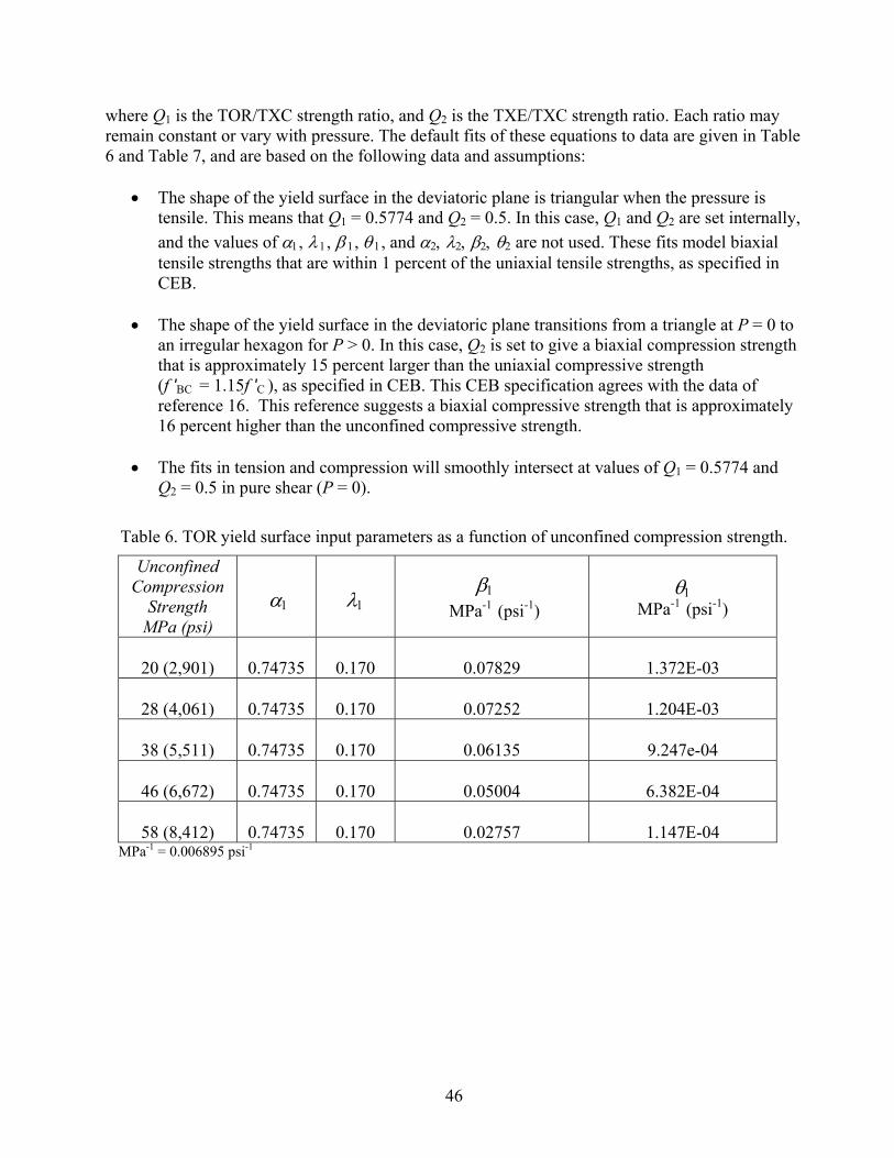
46

where Q1 is the TOR/TXC strength ratio, and Q2 is the TXE/TXC strength ratio. Each ratio may remain constant or vary with pressure. The default fits of these equations to data are given in Table 6 and Table 7, and are based on the following data and assumptions:

• The shape of the yield surface in the deviatoric plane is triangular when the pressure is tensile. This means that Q1 = 0.5774 and Q2 = 0.5. In this case, Q1 and Q2 are set internally, and the values of α1, λ 1, β 1, θ 1, and α2, λ2, β2, θ2 are not used. These fits model biaxial tensile strengths that are within 1 percent of the uniaxial tensile strengths, as specified in CEB.

• The shape of the yield surface in the deviatoric plane transitions from a triangle at P = 0 to an irregular hexagon for P > 0. In this case, Q2 is set to give a biaxial compression strength that is approximately 15 percent larger than the uniaxial compressive strength (f 'BC = 1.15f 'C ), as specified in CEB. This CEB specification agrees with the data of reference 16. This reference suggests a biaxial compressive strength that is approximately 16 percent higher than the unconfined compressive strength.

• The fits in tension and compression will smoothly intersect at values of Q1 = 0.5774 and Q2 = 0.5 in pure shear (P = 0).

Table 6. TOR yield surface input parameters as a function of unconfined compression strength.

Unconfined Compression

Strength MPa (psi)

α1

λ1

β1

MPa-1 (psi-1) θ1

MPa-1 (psi-1)

20 (2,901)

0.74735

0.170

0.07829

1.372E-03

28 (4,061)

0.74735

0.170

0.07252

1.204E-03

38 (5,511)

0.74735

0.170

0.06135

9.247e-04

46 (6,672)

0.74735

0.170

0.05004

6.382E-04

58 (8,412)

0.74735

0.170

0.02757

1.147E-04

MPa-1 = 0.006895 psi-1

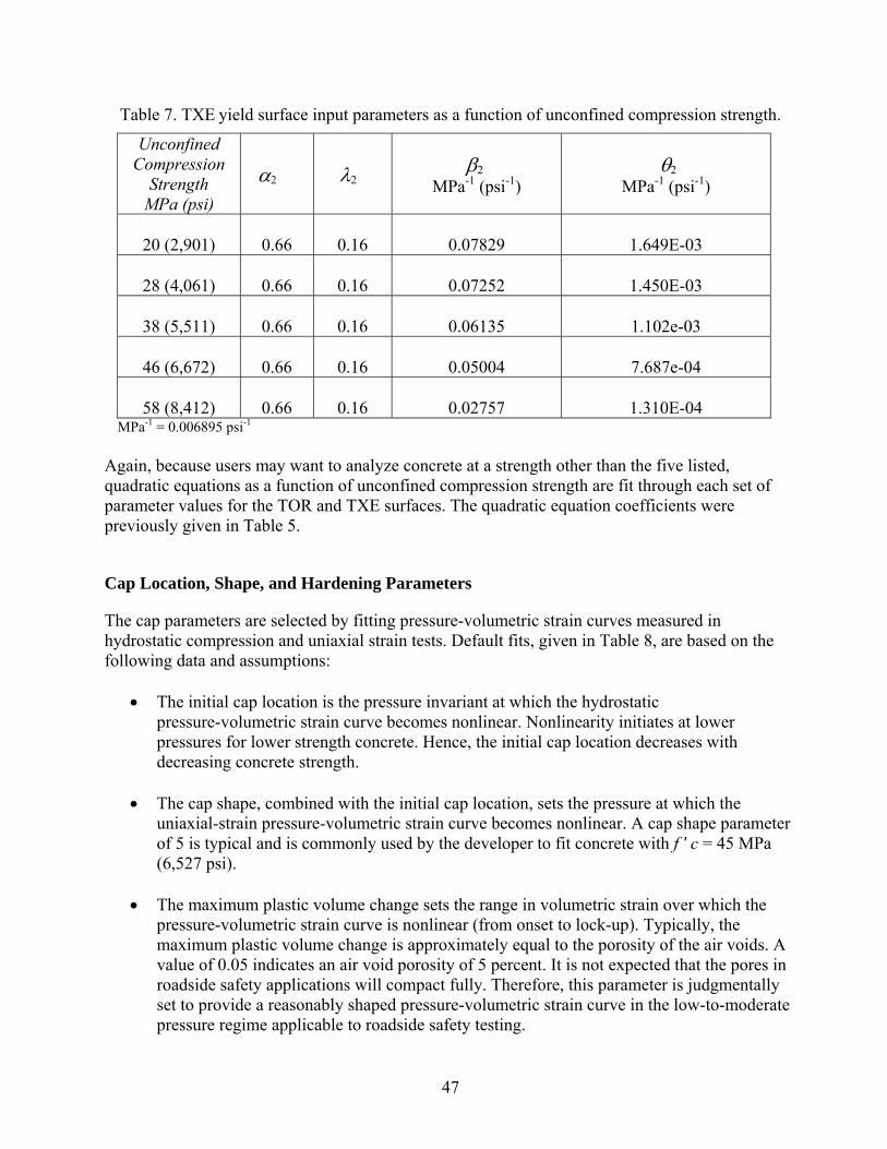
47

Table 7. TXE yield surface input parameters as a function of unconfined compression strength.

Unconfined Compression

Strength MPa (psi)

α2 λ2 β2

MPa-1 (psi-1) θ2

MPa-1 (psi-1)

20 (2,901)

0.66

0.16

0.07829

1.649E-03

28 (4,061)

0.66

0.16

0.07252

1.450E-03

38 (5,511)

0.66

0.16

0.06135

1.102e-03

46 (6,672)

0.66

0.16

0.05004

7.687e-04

58 (8,412)

0.66

0.16

0.02757

1.310E-04

MPa-1 = 0.006895 psi-1

Again, because users may want to analyze concrete at a strength other than the five listed, quadratic equations as a function of unconfined compression strength are fit through each set of parameter values for the TOR and TXE surfaces. The quadratic equation coefficients were previously given in Table 5.

Cap Location, Shape, and Hardening Parameters

The cap parameters are selected by fitting pressure-volumetric strain curves measured in hydrostatic compression and uniaxial strain tests. Default fits, given in Table 8, are based on the following data and assumptions:

• The initial cap location is the pressure invariant at which the hydrostatic

pressure-volumetric strain curve becomes nonlinear. Nonlinearity initiates at lower pressures for lower strength concrete. Hence, the initial cap location decreases with decreasing concrete strength.

• The cap shape, combined with the initial cap location, sets the pressure at which the

uniaxial-strain pressure-volumetric strain curve becomes nonlinear. A cap shape parameter of 5 is typical and is commonly used by the developer to fit concrete with f ' c = 45 MPa (6,527 psi).

• The maximum plastic volume change sets the range in volumetric strain over which the

pressure-volumetric strain curve is nonlinear (from onset to lock-up). Typically, the maximum plastic volume change is approximately equal to the porosity of the air voids. A value of 0.05 indicates an air void porosity of 5 percent. It is not expected that the pores in roadside safety applications will compact fully. Therefore, this parameter is judgmentally set to provide a reasonably shaped pressure-volumetric strain curve in the low-to-moderate pressure regime applicable to roadside safety testing.

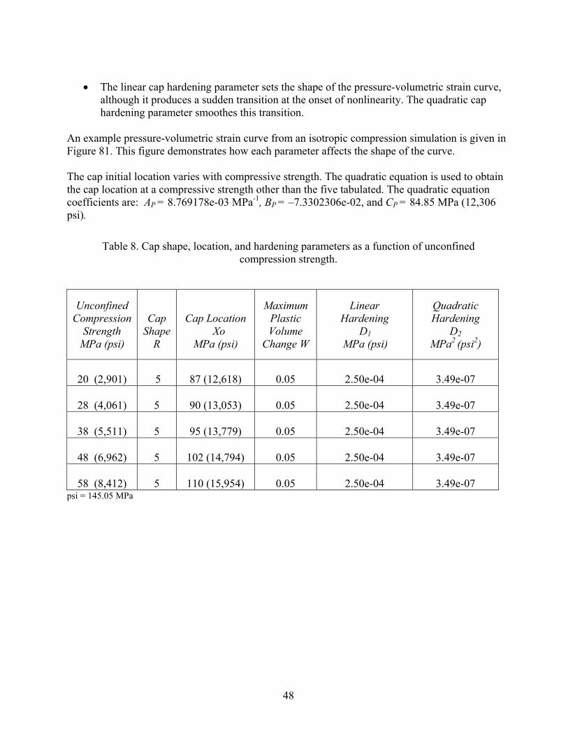
48

• The linear cap hardening parameter sets the shape of the pressure-volumetric strain curve,

although it produces a sudden transition at the onset of nonlinearity. The quadratic cap hardening parameter smoothes this transition.

An example pressure-volumetric strain curve from an isotropic compression simulation is given in Figure 81. This figure demonstrates how each parameter affects the shape of the curve. The cap initial location varies with compressive strength. The quadratic equation is used to obtain the cap location at a compressive strength other than the five tabulated. The quadratic equation coefficients are: AP = 8.769178e-03 MPa-1, BP = –7.3302306e-02, and CP = 84.85 MPa (12,306 psi).

Table 8. Cap shape, location, and hardening parameters as a function of unconfined compression strength.

Unconfined Compression

Strength MPa (psi)

Cap

ShapeR

Cap Location

Xo MPa (psi)

Maximum Plastic Volume

Change W

Linear Hardening

D1 MPa (psi)

Quadratic Hardening

D2 MPa2 (psi2)

20 (2,901)

5

87 (12,618)

0.05

2.50e-04

3.49e-07

28 (4,061)

5

90 (13,053)

0.05

2.50e-04

3.49e-07

38 (5,511)

5

95 (13,779)

0.05

2.50e-04

3.49e-07

48 (6,962)

5

102 (14,794)

0.05

2.50e-04

3.49e-07

58 (8,412)

5

110 (15,954)

0.05

2.50e-04

3.49e-07

psi = 145.05 MPa

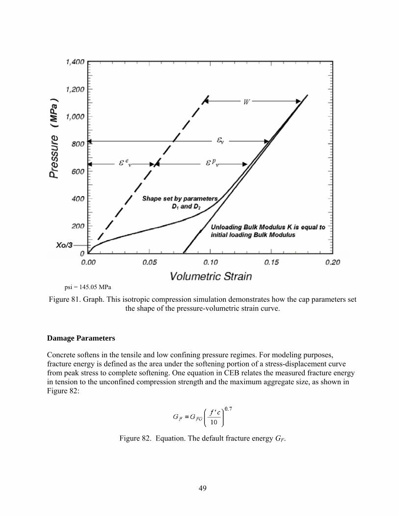
49

psi = 145.05 MPa

Figure 81. Graph. This isotropic compression simulation demonstrates how the cap parameters set the shape of the pressure-volumetric strain curve.

Damage Parameters

Concrete softens in the tensile and low confining pressure regimes. For modeling purposes, fracture energy is defined as the area under the softening portion of a stress-displacement curve from peak stress to complete softening. One equation in CEB relates the measured fracture energy in tension to the unconfined compression strength and the maximum aggregate size, as shown in Figure 82:

Figure 82. Equation. The default fracture energy GF.

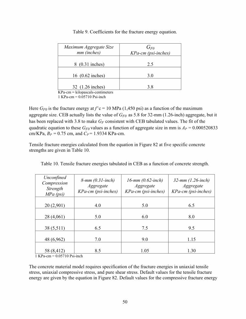
50

Table 9. Coefficients for the fracture energy equation.

Maximum Aggregate Size

mm (inches) GF0

KPa-cm (psi-inches)

8 (0.31 inches)

2.5

16 (0.62 inches)

3.0

32 (1.26 inches)

3.8 KPa-cm = kilopascals-centimeters 1 KPa-cm = 0.05710 Psi-inch

Here GF0 is the fracture energy at f ′c = 10 MPa (1,450 psi) as a function of the maximum aggregate size. CEB actually lists the value of GF0 as 5.8 for 32-mm (1.26-inch) aggregate, but it has been replaced with 3.8 to make GF consistent with CEB tabulated values. The fit of the quadratic equation to these GF0 values as a function of aggregate size in mm is AP = 0.000520833 cm/KPa, BP = 0.75 cm, and CP = 1.9334 KPa-cm. Tensile fracture energies calculated from the equation in Figure 82 at five specific concrete strengths are given in Table 10.

Table 10. Tensile fracture energies tabulated in CEB as a function of concrete strength.

Unconfined

Compression Strength

MPa (psi)

8-mm (0.31-inch) Aggregate

KPa-cm (psi-inches)

16-mm (0.62-inch) Aggregate

KPa-cm (psi-inches)

32-mm (1.26-inch) Aggregate

KPa-cm (psi-inches)

20 (2,901)

4.0

5.0

6.5

28 (4,061)

5.0

6.0

8.0

38 (5,511)

6.5

7.5

9.5

48 (6,962)

7.0

9.0

1.15

58 (8,412)

8.5

1.05

1.30

1 KPa-cm = 0.05710 Psi-inch The concrete material model requires specification of the fracture energies in uniaxial tensile stress, uniaxial compressive stress, and pure shear stress. Default values for the tensile fracture energy are given by the equation in Figure 82. Default values for the compressive fracture energy

51

ε&

are set at 100 times the tensile fracture energy. Default values for the shear fracture energy are set equal to the tensile fracture energy. Other input parameters required are the brittle and ductile damage thresholds and the maximum damage levels:

• Each damage threshold sets the elastic strain energy level at which softening initiates. The brittle damage threshold is set equal to the elastic strain energy level in unconfined tension at peak stress. The ductile damage threshold is set equal to the elastic strain energy level in unconfined compression at peak stress.

• The shape of the softening curves is set by the parameters B and D. A value of B = 100.0 is set in compression for gradual initial softening (flat top). A value of D = 0.1 is set in tension for brittle initial softening (pointed top).

• The maximum damage parameters set the maximum damage levels attained in unconfined compression and tension. The maximum damage levels are set equal to 0.99 for both brittle and ductile formulations.

Strain Rate Parameters

Concrete exhibits an increase in strength with increasing strain rate (refer to Figure 13 and Figure 14). Data are typically reported in terms of the ratio of dynamic to static strength, called the dynamic increase factor (DIF). CEB provides specifications for the DIF, as discussed in appendix D. However, the CEB specifications are not a good fit to the tensile data previously shown in Figure 14. Therefore, the DIF used and shown in Figure 83 is based on the developer’s experience on various defense contracts, particularly for concrete with strength around f 'c = 45 MPa (6,527 psi). These specifications provide a good fit to both the tension and compression data previously shown in Figure 13 and Figure 14. DIF specifications are approximately met by running numerous calculations and selecting the viscoplastic rate effects parameters via a trial and error method. The viscoplastic parameters are applied to the plasticity, damage, and fracture energy formulations. These parameters are η0t and nt for fitting uniaxial tensile stress data, and η0c and nc for fitting uniaxial compression data. Quadratic equation coefficients are dependent on the unconfined compression strength, but are independent of the aggregate size. The default parameters in tension are nt = 0.48, with quadratic equation coefficients for η0t of AP = 8.0614774E-13, BP = −9.77736719E-10, and CP = 5.0752351E-05 for time in seconds and stress in pounds per square inch. The default parameters in compression are nc = 0.78, with quadratic equation coefficients for η0c of AP = 1.2772337-11, BP = −1.0613722E-07, and CP = 3.203497-04. Rate effects parameters in pure shear stress are set equal to those in tension via Srate = 1. The overstress limits in tension (overt) and compression (overc) limit rate effects at high strain rates ( > 100). The overstress quadratic equation coefficients for overt are AP = 1.309663E-02

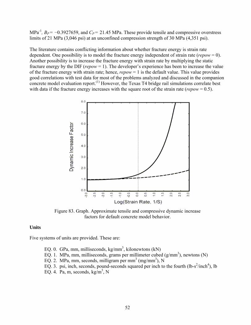
52

MPa-1, BP = −0.3927659, and CP = 21.45 MPa. These provide tensile and compressive overstress limits of 21 MPa (3,046 psi) at an unconfined compression strength of 30 MPa (4,351 psi).

The literature contains conflicting information about whether fracture energy is strain rate dependent. One possibility is to model the fracture energy independent of strain rate (repow = 0). Another possibility is to increase the fracture energy with strain rate by multiplying the static fracture energy by the DIF (repow = 1). The developer’s experience has been to increase the value of the fracture energy with strain rate; hence, repow = 1 is the default value. This value provides good correlations with test data for most of the problems analyzed and discussed in the companion concrete model evaluation report.(1) However, the Texas T4 bridge rail simulations correlate best with data if the fracture energy increases with the square root of the strain rate (repow = 0.5).

Figure 83. Graph. Approximate tensile and compressive dynamic increase

factors for default concrete model behavior.

Units

Five systems of units are provided. These are: EQ. 0. GPa, mm, milliseconds, kg/mm3, kilonewtons (kN) EQ. 1. MPa, mm, milliseconds, grams per millimeter cubed (g/mm3), newtons (N) EQ. 2. MPa, mm, seconds, milligram per mm3 (mg/mm3), N EQ. 3. psi, inch, seconds, pound-seconds squared per inch to the fourth (lb-s2/inch4), lb EQ. 4. Pa, m, seconds, kg/m3, N

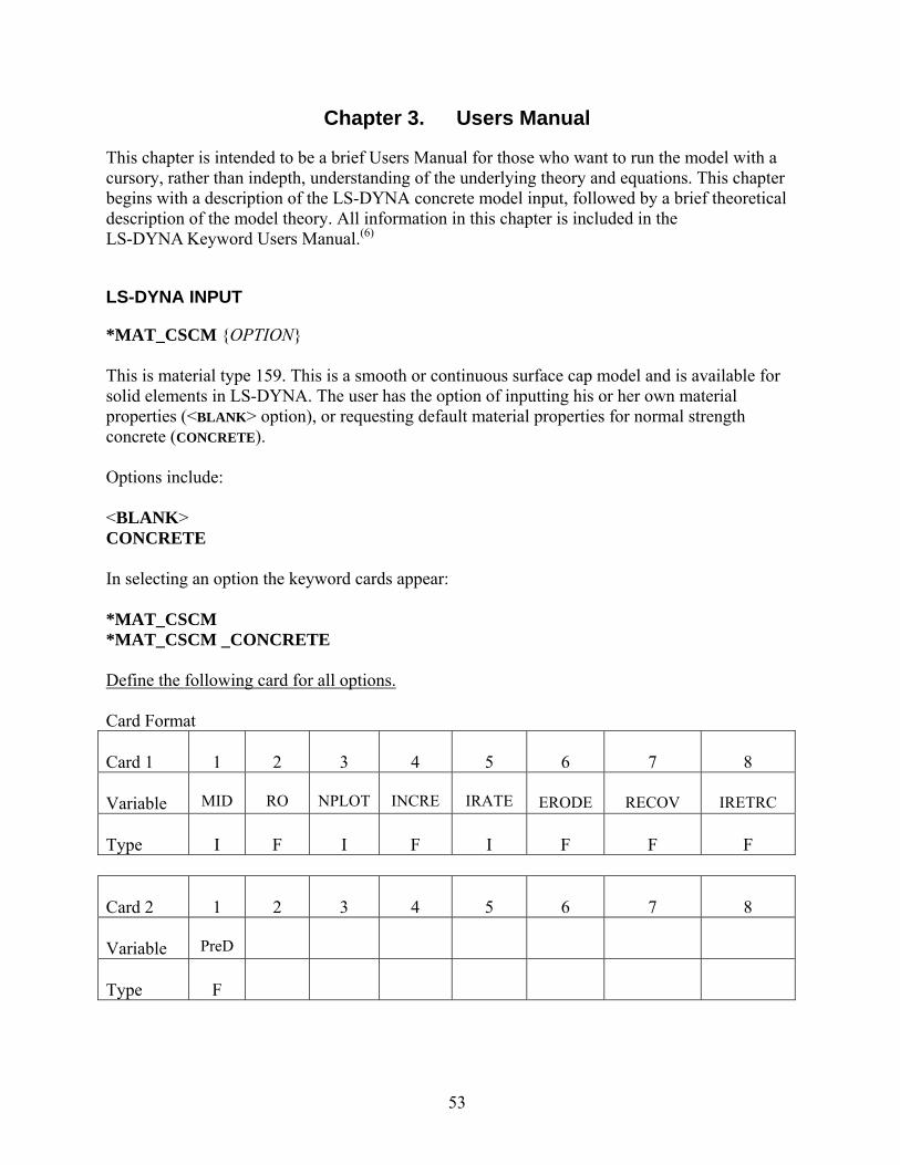
53

Chapter 3. Users Manual

This chapter is intended to be a brief Users Manual for those who want to run the model with a cursory, rather than indepth, understanding of the underlying theory and equations. This chapter begins with a description of the LS-DYNA concrete model input, followed by a brief theoretical description of the model theory. All information in this chapter is included in the LS-DYNA Keyword Users Manual.(6)

LS-DYNA INPUT

*MAT_CSCM {OPTION} This is material type 159. This is a smooth or continuous surface cap model and is available for solid elements in LS-DYNA. The user has the option of inputting his or her own material properties (<BLANK> option), or requesting default material properties for normal strength concrete (CONCRETE). Options include: <BLANK> CONCRETE In selecting an option the keyword cards appear: *MAT_CSCM *MAT_CSCM _CONCRETE Define the following card for all options. Card Format Card 1

1

2

3

4

5

6

7

8

Variable

MID

RO

NPLOT

INCRE

IRATE

ERODE

RECOV

IRETRC

Type

I

F

I

F

I

F

F

F

Card 2

1

2

3

4

5

6

7

8

Variable

PreD

Type

F

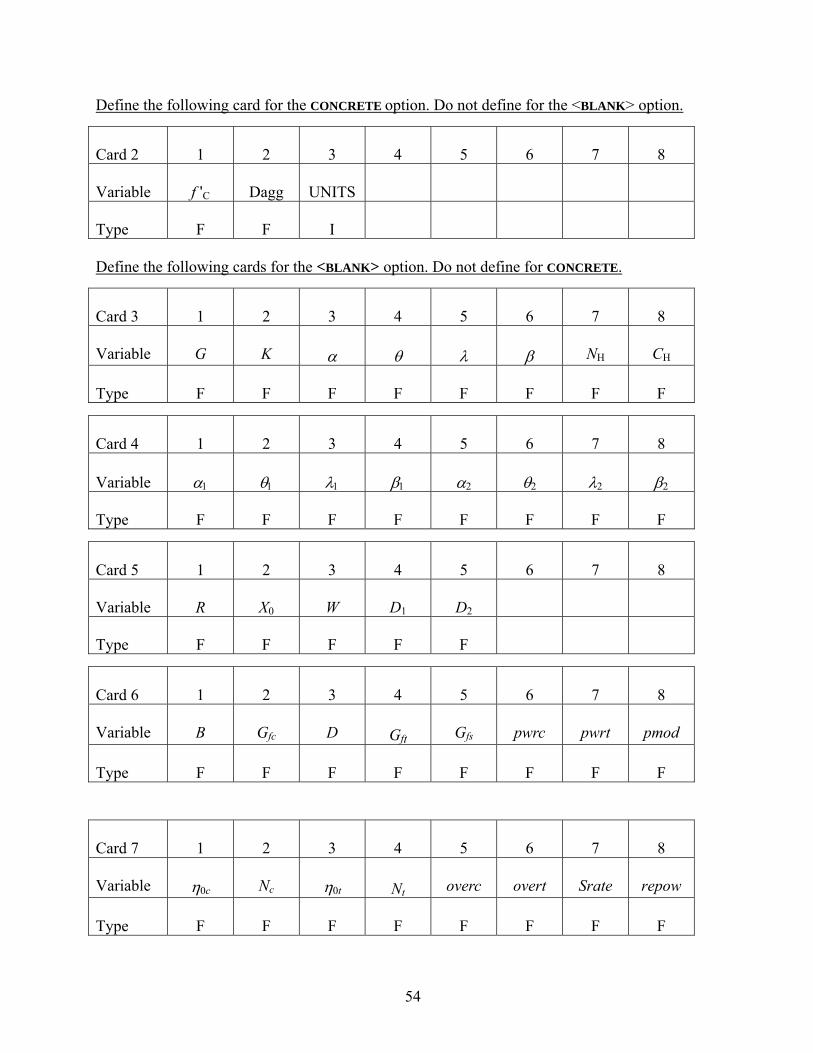
54

Define the following card for the CONCRETE option. Do not define for the <BLANK> option.

Card 2

1

2

3

4

5

6

7

8

Variable

f 'C

Dagg

UNITS

Type

F

F

I

Define the following cards for the <BLANK> option. Do not define for CONCRETE.

Card 3

1

2

3

4

5

6

7

8

Variable

G

K

α

θ

λ

β

NH

CH

Type

F

F

F

F

F

F

F

F

Card 4

1

2

3

4

5

6

7

8

Variable α1 θ1 λ1 β1 α2 θ2 λ2

β2 Type

F

F

F

F

F

F

F

F

Card 5

1

2

3

4

5

6

7

8

Variable

R

X0

W

D1

D2

Type

F

F

F

F

F

Card 6

1

2

3

4

5

6

7

8

Variable

B

Gfc

D

Gft

Gfs

pwrc

pwrt

pmod

Type

F

F

F

F

F

F

F

F

Card 7

1

2

3

4

5

6

7

8

Variable

η0c

Nc

η0t

Nt

overc

overt

Srate

repow

Type

F

F

F

F

F

F

F

F

55

Define for all options. Variable Description MID Material identification. A unique number must be chosen. RO Mass density. NPLOT Plotting options:

EQ. 1. Maximum of brittle and ductile damage (default). EQ. 2 Maximum of brittle and ductile damage, with recovery of brittle damage. EQ. 3. Brittle damage. EQ. 4. Ductile damage. EQ. 5. κ (intersection of cap with shear surface). EQ. 6. X0 (intersection of cap with pressure axis). EQ. 7. p

vε (plastic volume strain).

INCRE Maximum strain increment for subincrementation. If left blank, a default value is set during initialization based upon the shear strength and stiffness.

IRATE Rate effects options: EQ. 0. Rate effects model turned off (default). EQ. 1. Rate effects model turned on.

ERODE Elements erode when damage exceeds 0.99 and the maximum principal strain exceeds 1-ERODE. For erosion that is independent of strain, set ERODE equal to 1.0. Erosion does not occur if ERODE is less than 1.0.

RECOV The modulus is recovered in compression when RECOV is equal to 0 (default). The

modulus remains at the brittle damage level when RECOV is equal to 1. Partial recovery is modeled for values of RECOV between 0 and 1.

IRETRC Cap retraction option:

EQ. 0. Cap does not retract (default). EQ. 1. Cap retracts.

PreD Preexisting damage (0 ≤ PreD < 1). If left blank, the default is zero (no preexisiting

damage).

56

Define for CONCRETE option. Variable Description

f 'C Unconfined compression strength. If left blank, default is 30 MPa (4,351 psi). Dagg Maximum aggregate size. If left blank, default is 19 mm (0.75 inch). UNITS Units options: EQ. 0. GPa, mm, milliseconds, kg/mm3, kN EQ. 1. MPa, mm, milliseconds, g/mm3, N EQ. 2. MPa, mm, seconds, mg/mm3, N EQ. 3. psi, inch, seconds, lb-s2/inch4, lb EQ. 4. Pa, m, seconds, kg/m3, N Remarks:

Default concrete input parameters are for normal strength concrete with unconfined compression strengths between about 20 and 58 MPa (2,901 and 8,412 psi).

Define for <BLANK> option only. Variable Description G shear modulus K bulk modulus α TXC surface constant term θ TXC surface linear term λ TXC surface nonlinear term β TXC surface exponent α1 TOR surface constant term θ1 TOR surface linear term λ1 TOR surface nonlinear term β1 TOR surface exponent α2 TXE surface constant term θ2 TXE surface linear term λ2 TXE surface nonlinear term β2 TXE surface exponent NH hardening initiation CH hardening rate

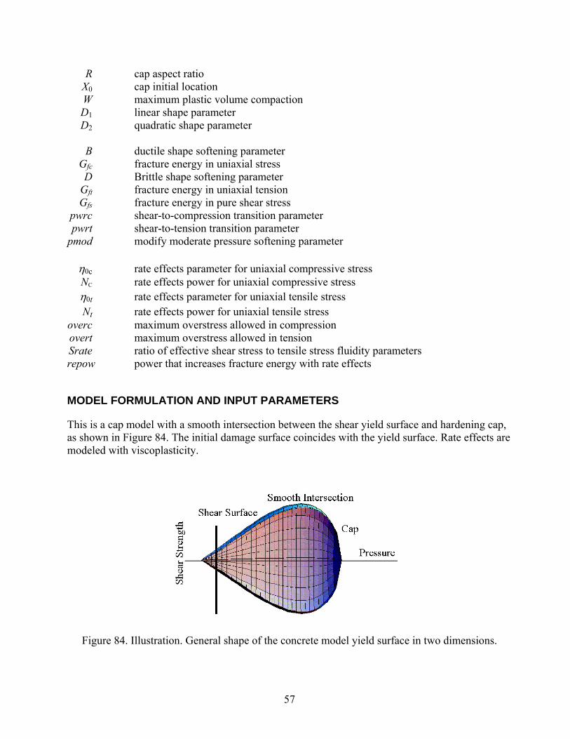
57

R cap aspect ratio X0 cap initial location W maximum plastic volume compaction D1 linear shape parameter D2 quadratic shape parameter B ductile shape softening parameter Gfc fracture energy in uniaxial stress D Brittle shape softening parameter Gft fracture energy in uniaxial tension Gfs fracture energy in pure shear stress pwrc shear-to-compression transition parameter pwrt shear-to-tension transition parameter pmod modify moderate pressure softening parameter η0c rate effects parameter for uniaxial compressive stress NC rate effects power for uniaxial compressive stress η0t rate effects parameter for uniaxial tensile stress Nt rate effects power for uniaxial tensile stress overc maximum overstress allowed in compression overt maximum overstress allowed in tension Srate ratio of effective shear stress to tensile stress fluidity parameters repow power that increases fracture energy with rate effects

MODEL FORMULATION AND INPUT PARAMETERS

This is a cap model with a smooth intersection between the shear yield surface and hardening cap, as shown in Figure 84. The initial damage surface coincides with the yield surface. Rate effects are modeled with viscoplasticity.

Figure 84. Illustration. General shape of the concrete model yield surface in two dimensions.

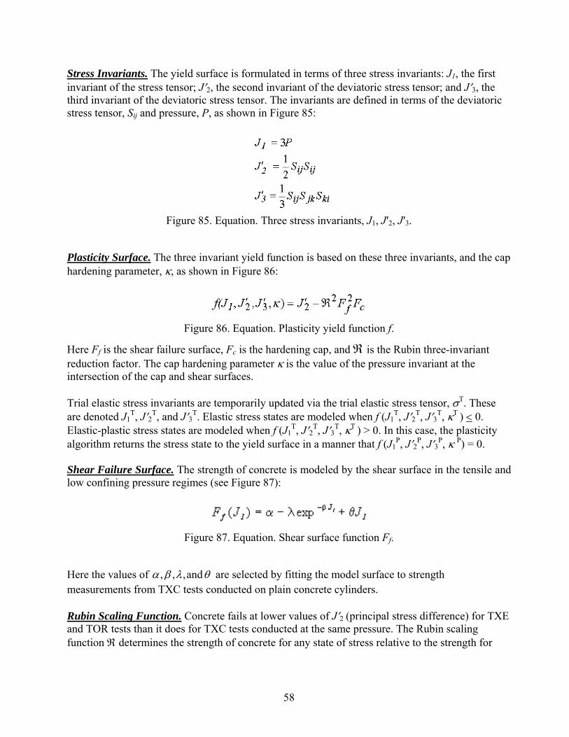
58

Stress Invariants. The yield surface is formulated in terms of three stress invariants: J1, the first invariant of the stress tensor; J′2, the second invariant of the deviatoric stress tensor; and J′3, the third invariant of the deviatoric stress tensor. The invariants are defined in terms of the deviatoric stress tensor, Sij and pressure, P, as shown in Figure 85:

Figure 85. Equation. Three stress invariants, J1, J′2, J′3.

Plasticity Surface. The three invariant yield function is based on these three invariants, and the cap hardening parameter, κ, as shown in Figure 86:

Figure 86. Equation. Plasticity yield function f.

Here Ff is the shear failure surface, Fc is the hardening cap, and ℜ is the Rubin three-invariant reduction factor. The cap hardening parameter κ is the value of the pressure invariant at the intersection of the cap and shear surfaces. Trial elastic stress invariants are temporarily updated via the trial elastic stress tensor, σT. These are denoted J1

T, J′2T, and J′3T. Elastic stress states are modeled when f (J1T, J′2T, J′3T, κΤ ) < 0.

Elastic-plastic stress states are modeled when f (J1T, J′2T, J′3T, κΤ ) > 0. In this case, the plasticity

algorithm returns the stress state to the yield surface in a manner that f (J1P, J′2P, J′3P, κ P) = 0.

Shear Failure Surface. The strength of concrete is modeled by the shear surface in the tensile and low confining pressure regimes (see Figure 87):

Figure 87. Equation. Shear surface function Ff.

Here the values of θλβα and,,, are selected by fitting the model surface to strength measurements from TXC tests conducted on plain concrete cylinders. Rubin Scaling Function. Concrete fails at lower values of J′2 (principal stress difference) for TXE and TOR tests than it does for TXC tests conducted at the same pressure. The Rubin scaling function ℜ determines the strength of concrete for any state of stress relative to the strength for

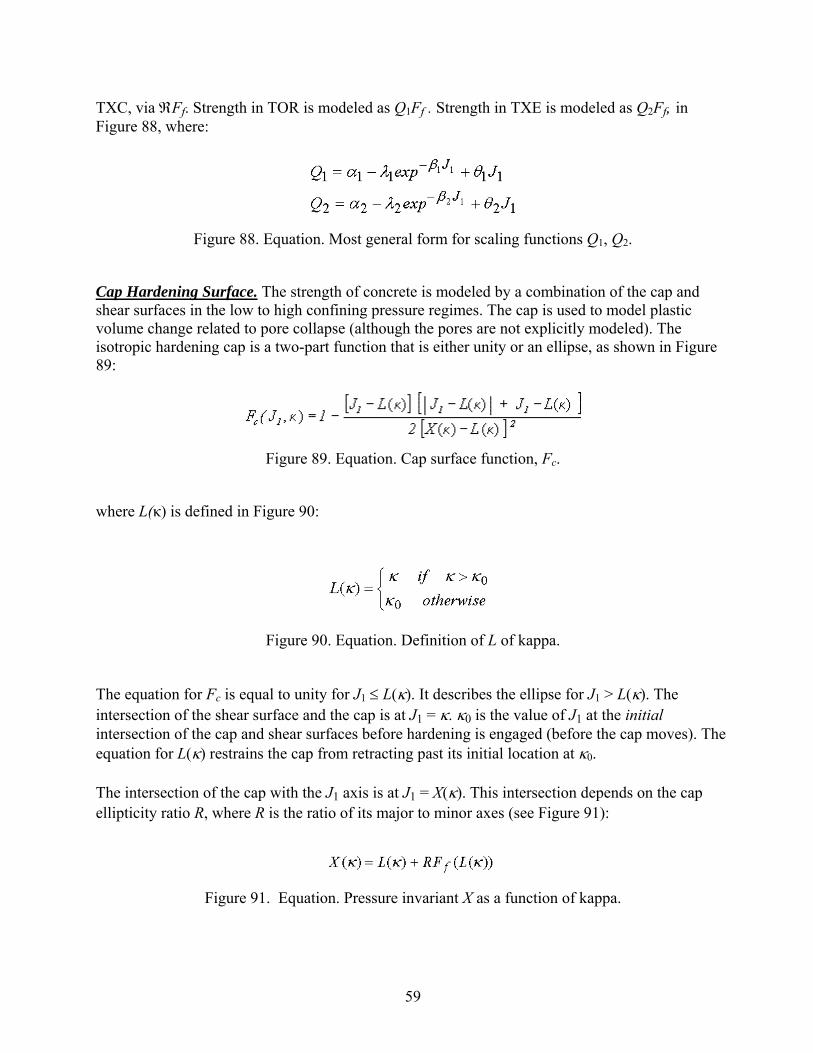
59

TXC, via ℜFf. Strength in TOR is modeled as Q1Ff . Strength in TXE is modeled as Q2Ff, in Figure 88, where:

Figure 88. Equation. Most general form for scaling functions Q1, Q2.

Cap Hardening Surface. The strength of concrete is modeled by a combination of the cap and shear surfaces in the low to high confining pressure regimes. The cap is used to model plastic volume change related to pore collapse (although the pores are not explicitly modeled). The isotropic hardening cap is a two-part function that is either unity or an ellipse, as shown in Figure 89:

Figure 89. Equation. Cap surface function, Fc.

where L(κ) is defined in Figure 90:

Figure 90. Equation. Definition of L of kappa.

The equation for Fc is equal to unity for J1 ≤ L(κ). It describes the ellipse for J1 > L(κ). The intersection of the shear surface and the cap is at J1 = κ. κ0 is the value of J1 at the initial intersection of the cap and shear surfaces before hardening is engaged (before the cap moves). The equation for L(κ) restrains the cap from retracting past its initial location at κ0. The intersection of the cap with the J1 axis is at J1 = X(κ). This intersection depends on the cap ellipticity ratio R, where R is the ratio of its major to minor axes (see Figure 91):

Figure 91. Equation. Pressure invariant X as a function of kappa.

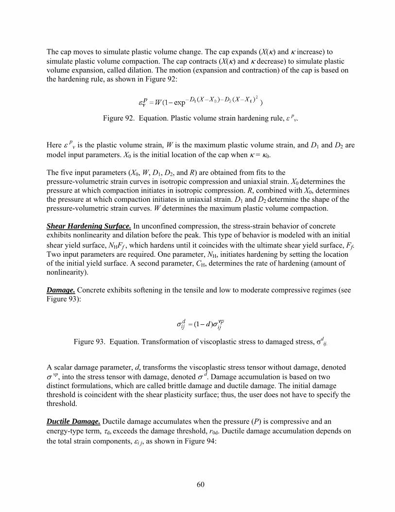
60

The cap moves to simulate plastic volume change. The cap expands (X(κ) and κ increase) to simulate plastic volume compaction. The cap contracts (X(κ) and κ decrease) to simulate plastic volume expansion, called dilation. The motion (expansion and contraction) of the cap is based on the hardening rule, as shown in Figure 92:

Figure 92. Equation. Plastic volume strain hardening rule, ε pv.

Here ε pv is the plastic volume strain, W is the maximum plastic volume strain, and D1 and D2 are model input parameters. X0 is the initial location of the cap when κ = κ0. The five input parameters (X0, W, D1, D2, and R) are obtained from fits to the pressure-volumetric strain curves in isotropic compression and uniaxial strain. X0 determines the pressure at which compaction initiates in isotropic compression. R, combined with X0, determines the pressure at which compaction initiates in uniaxial strain. D1 and D2 determine the shape of the pressure-volumetric strain curves. W determines the maximum plastic volume compaction. Shear Hardening Surface. In unconfined compression, the stress-strain behavior of concrete exhibits nonlinearity and dilation before the peak. This type of behavior is modeled with an initial shear yield surface, NHFf , which hardens until it coincides with the ultimate shear yield surface, Ff. Two input parameters are required. One parameter, NH, initiates hardening by setting the location of the initial yield surface. A second parameter, CH, determines the rate of hardening (amount of nonlinearity). Damage. Concrete exhibits softening in the tensile and low to moderate compressive regimes (see Figure 93):

Figure 93. Equation. Transformation of viscoplastic stress to damaged stress, σd

ij.

A scalar damage parameter, d, transforms the viscoplastic stress tensor without damage, denoted σ vp, into the stress tensor with damage, denoted σ d. Damage accumulation is based on two distinct formulations, which are called brittle damage and ductile damage. The initial damage threshold is coincident with the shear plasticity surface; thus, the user does not have to specify the threshold. Ductile Damage. Ductile damage accumulates when the pressure (P) is compressive and an energy-type term, τd, exceeds the damage threshold, r0d. Ductile damage accumulation depends on the total strain components, εi j, as shown in Figure 94:

61

Figure 94. Equation. Ductile damage accumulation, τ d.

The stress components σij are the elasto-plastic stresses (with kinematic hardening) calculated before application of damage and rate effects. Brittle Damage. Brittle damage accumulates when the pressure is tensile and an energy-type term, τb, exceeds the damage threshold, r0b. Brittle damage accumulation depends on the maximum principal strain, ε max, as shown in Figure 95:

Figure 95. Equation. Brittle damage accumulation, τb.

Softening Function. As damage accumulates, the damage parameter d increases from an initial value of zero, towards a maximum value of 1, via Figures 96 and 97:

Figure 96. Equation. Brittle damage, d of τb.

Figure 97. Equation. Ductile damage, d of τd.

The damage parameter applied to the six stresses is equal to the current maximum of the brittle or ductile damage parameter. The parameters A and B or C and D set the shape of the softening curve plotted as stress-displacement or stress-strain. The parameter dmax is the maximum damage level that can be attained. It is calculated internally and is less than 1 at moderate confining pressures. The compressive softening parameter, A, may also be reduced with confinement, using the input parameter pmod, as shown in Figure 98:

Figure 98. Equation. Reduction of A with confinement.

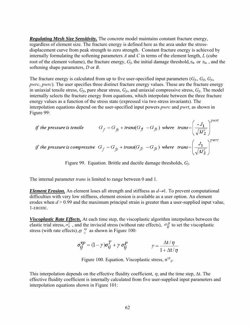
62

Regulating Mesh Size Sensitivity. The concrete model maintains constant fracture energy, regardless of element size. The fracture energy is defined here as the area under the stress-displacement curve from peak strength to zero strength. Constant fracture energy is achieved by internally formulating the softening parameters A and C in terms of the element length, L (cube root of the element volume), the fracture energy, Gf, the initial damage threshold,τ0t or τ0c , and the softening shape parameters, D or B. The fracture energy is calculated from up to five user-specified input parameters (Gfc, Gft, Gfs, pwrc, pwrc). The user specifies three distinct fracture energy values. These are the fracture energy in uniaxial tensile stress, Gft, pure shear stress, Gfs, and uniaxial compressive stress, Gfc. The model internally selects the fracture energy from equations, which interpolate between the three fracture energy values as a function of the stress state (expressed via two stress invariants). The interpolation equations depend on the user-specified input powers pwrc and pwrt, as shown in Figure 99:

Figure 99. Equation. Brittle and ductile damage thresholds, Gf.

The internal parameter trans is limited to range between 0 and 1. Element Erosion. An element loses all strength and stiffness as d→1. To prevent computational difficulties with very low stiffness, element erosion is available as a user option. An element erodes when d > 0.99 and the maximum principal strain is greater than a user-supplied input value, 1-ERODE. Viscoplastic Rate Effects. At each time step, the viscoplastic algorithm interpolates between the elastic trial stress, , and the inviscid stress (without rate effects), , to set the viscoplastic stress (with rate effects), : as shown in Figure 100:

Figure 100. Equation. Viscoplastic stress, σvp

ij.

This interpolation depends on the effective fluidity coefficient, η, and the time step, Δt. The effective fluidity coefficient is internally calculated from five user-supplied input parameters and interpolation equations shown in Figure 101:

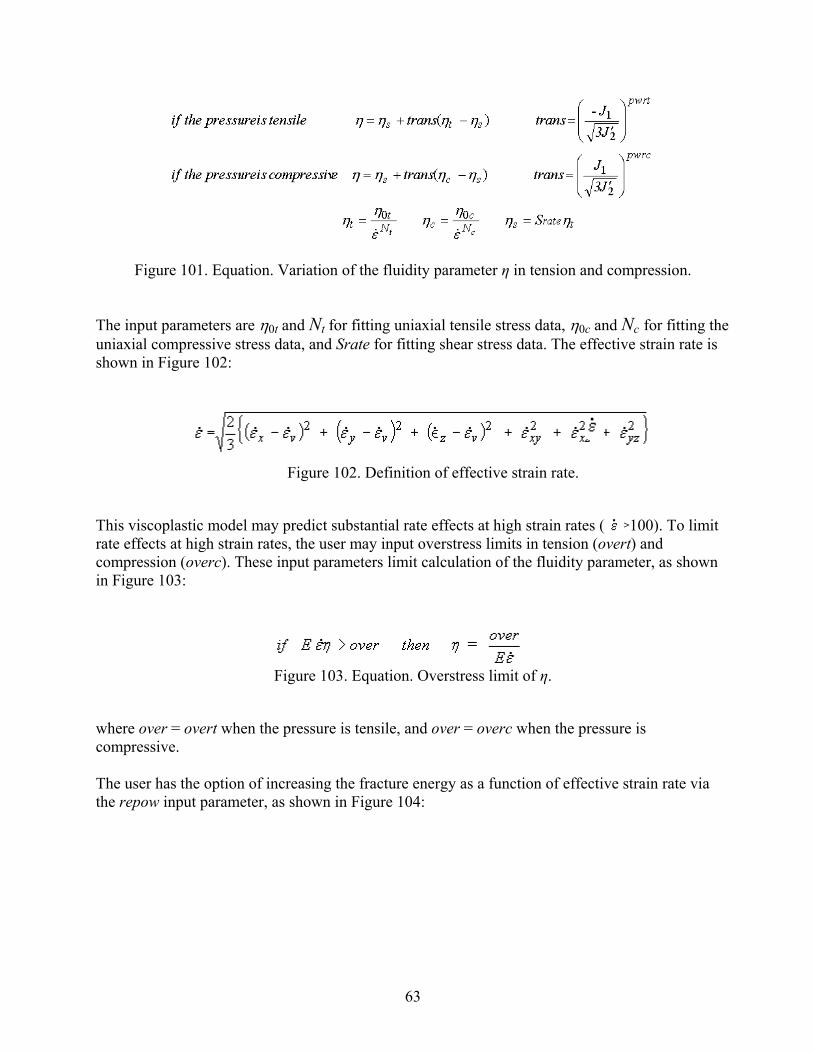
63

Figure 101. Equation. Variation of the fluidity parameter η in tension and compression.

The input parameters are η0t and Nt for fitting uniaxial tensile stress data, η0c and Nc for fitting the uniaxial compressive stress data, and Srate for fitting shear stress data. The effective strain rate is shown in Figure 102:

Figure 102. Definition of effective strain rate.

This viscoplastic model may predict substantial rate effects at high strain rates ( >100). To limit rate effects at high strain rates, the user may input overstress limits in tension (overt) and compression (overc). These input parameters limit calculation of the fluidity parameter, as shown in Figure 103:

Figure 103. Equation. Overstress limit of η.

where over = overt when the pressure is tensile, and over = overc when the pressure is compressive. The user has the option of increasing the fracture energy as a function of effective strain rate via the repow input parameter, as shown in Figure 104:

64

Figure 104. Equation. Fracture energy with rate effects, .

Here is the fracture energy enhanced by rate effects, and f′ is the yield strength before application of rate effects (which is calculated internally by the model). The term in brackets is greater than, or equal to 1, and is the approximate ratio of the dynamic to static strength.

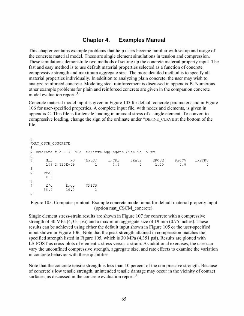
65

Chapter 4. Examples Manual

This chapter contains example problems that help users become familiar with set up and usage of the concrete material model. These are single element simulations in tension and compression. These simulations demonstrate two methods of setting up the concrete material property input. The fast and easy method is to use default material properties selected as a function of concrete compressive strength and maximum aggregate size. The more detailed method is to specify all material properties individually. In addition to analyzing plain concrete, the user may wish to analyze reinforced concrete. Modeling steel reinforcement is discussed in appendix B. Numerous other example problems for plain and reinforced concrete are given in the companion concrete model evaluation report.(1)

Concrete material model input is given in Figure 105 for default concrete parameters and in Figure 106 for user-specified properties. A complete input file, with nodes and elements, is given in appendix C. This file is for tensile loading in uniaxial stress of a single element. To convert to compressive loading, change the sign of the ordinate under *DEFINE_CURVE at the bottom of the file.

Figure 105. Computer printout. Example concrete model input for default material property input

(option mat_CSCM_concrete).

Single element stress-strain results are shown in Figure 107 for concrete with a compressive strength of 30 MPa (4,351 psi) and a maximum aggregate size of 19 mm (0.75 inches). These results can be achieved using either the default input shown in Figure 105 or the user-specified input shown in Figure 106. Note that the peak strength attained in compression matches the specified strength listed in Figure 105, which is 30 MPa (4,351 psi). Results are plotted with LS-POST as cross-plots of element z-stress versus z-strain. As additional exercises, the user can vary the unconfined compressive strength, aggregate size, and rate effects to examine the variation in concrete behavior with these quantities. Note that the concrete tensile strength is less than 10 percent of the compressive strength. Because of concrete’s low tensile strength, unintended tensile damage may occur in the vicinity of contact surfaces, as discussed in the concrete evaluation report.(1)

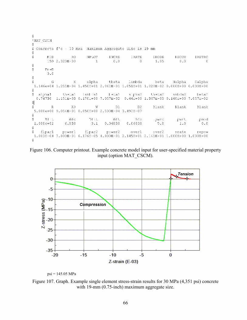
66

Figure 106. Computer printout. Example concrete model input for user-specified material property

input (option MAT_CSCM).

psi = 145.05 MPa

Figure 107. Graph. Example single element stress-strain results for 30 MPa (4,351 psi) concrete with 19-mm (0.75-inch) maximum aggregate size.

67

Appendix A. Modeling Softening

Two formulations the developer has employed to model softening are shown in Figures 108 and 109:

Figure 108. Equation. Old generic damage, small d of τ.

Figure 109. Equation. New generic damage, small d of τ.

The first formulation is the original one used by the developer in older versions of the smooth cap concrete model, as well as the soil model (MAT 147). The second formulation is an updated formulation used by the developer in the concrete model 159 discussed in this report, as well as the wood model (MAT 143).

The equation in Figure 109 has the same number of parameters as the equation in Figure 108, but provides a slightly different fit. Differences in the two softening functions are given in Figure 110 and Figure 111 for dmax = 1. Three different fits are generated for each function. One softening parameter is varied (A or B); the second is held constant (B or A). Note that the updated softening function can model a flat or steep descent upon initiation of damage, whereas the original softening function can only model a steep descent.

⎥⎥

⎦

⎤

⎢⎢

⎣

⎡−

−+

+=

−1(

exp1

1)()0rA

B

BB

dd maxττ

68

Figure 110. Graph. Behavior of the original softening function.

Figure 111. Graph. Behavior of the updated softening function.

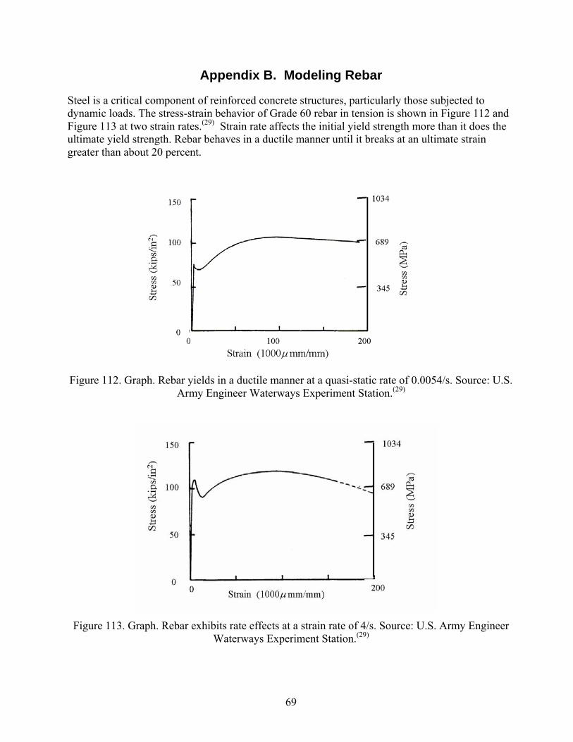
69

Appendix B. Modeling Rebar

Steel is a critical component of reinforced concrete structures, particularly those subjected to dynamic loads. The stress-strain behavior of Grade 60 rebar in tension is shown in Figure 112 and Figure 113 at two strain rates.(29) Strain rate affects the initial yield strength more than it does the ultimate yield strength. Rebar behaves in a ductile manner until it breaks at an ultimate strain greater than about 20 percent.

Figure 112. Graph. Rebar yields in a ductile manner at a quasi-static rate of 0.0054/s. Source: U.S.

Army Engineer Waterways Experiment Station.(29)

Figure 113. Graph. Rebar exhibits rate effects at a strain rate of 4/s. Source: U.S. Army Engineer

Waterways Experiment Station.(29)

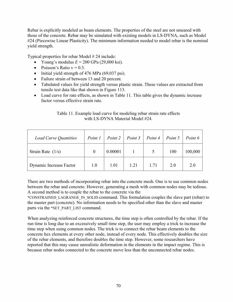
70

Rebar is explicitly modeled as beam elements. The properties of the steel are not smeared with those of the concrete. Rebar may be simulated with existing models in LS-DYNA, such as Model #24 (Piecewise Linear Plasticity). The minimum information needed to model rebar is the nominal yield strength. Typical properties for rebar Model # 24 include:

• Young’s modulus E = 200 GPa (29,000 ksi). • Poisson’s Ratio ν = 0.3. • Initial yield strength of 476 MPa (69,037 psi). • Failure strain of between 13 and 20 percent. • Tabulated values for yield strength versus plastic strain. These values are extracted from

tensile test data like that shown in Figure 113. • Load curve for rate effects, as shown in Table 11. This table gives the dynamic increase

factor versus effective strain rate.

Table 11. Example load curve for modeling rebar strain rate effects with LS-DYNA Material Model #24.

There are two methods of incorporating rebar into the concrete mesh. One is to use common nodes between the rebar and concrete. However, generating a mesh with common nodes may be tedious. A second method is to couple the rebar to the concrete via the *CONSTRAINED_LAGRANGE_IN_SOLID command. This formulation couples the slave part (rebar) to the master part (concrete). No information needs to be specified other than the slave and master parts via the *SET_PART_LIST command. When analyzing reinforced concrete structures, the time step is often controlled by the rebar. If the run time is long due to an excessively small time step, the user may employ a trick to increase the time step when using common nodes. The trick is to connect the rebar beam elements to the concrete hex elements at every other node, instead of every node. This effectively doubles the size of the rebar elements, and therefore doubles the time step. However, some researchers have reported that this may cause unrealistic deformation in the elements in the impact regime. This is because rebar nodes connected to the concrete move less than the unconnected rebar nodes.

Load Curve Quantities

Point 1

Point 2

Point 3

Point 4

Point 5

Point 6

Strain Rate (1/s)

0

0.00001

1

5

100

100,000

Dynamic Increase Factor

1.0

1.01

1.21

1.71

2.0

2.0

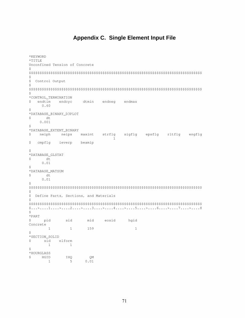
71

Appendix C. Single Element Input File

*KEYWORD *TITLE Unconfined Tension of Concrete $ $$$$$$$$$$$$$$$$$$$$$$$$$$$$$$$$$$$$$$$$$$$$$$$$$$$$$$$$$$$$$$$$$$$$$$$$$$$$$$$$ $ $ Control Output $ $$$$$$$$$$$$$$$$$$$$$$$$$$$$$$$$$$$$$$$$$$$$$$$$$$$$$$$$$$$$$$$$$$$$$$$$$$$$$$$$ $ *CONTROL_TERMINATION $ endtim endcyc dtmin endneg endmas 0.60 $ *DATABASE_BINARY_D3PLOT $ dt 0.001 $ *DATABASE_EXTENT_BINARY $ neiph neips maxint strflg sigflg epsflg rltflg engflg 1 $ cmpflg ieverp beamip $ *DATABASE_GLSTAT $ dt 0.01 $ *DATABASE_MATSUM $ dt 0.01 $ $$$$$$$$$$$$$$$$$$$$$$$$$$$$$$$$$$$$$$$$$$$$$$$$$$$$$$$$$$$$$$$$$$$$$$$$$$$$$$$$ $ $ Define Parts, Sections, and Materials $ $$$$$$$$$$$$$$$$$$$$$$$$$$$$$$$$$$$$$$$$$$$$$$$$$$$$$$$$$$$$$$$$$$$$$$$$$$$$$$$$ $...>....1....>....2....>....3....>....4....>....5....>....6....>....7....>....8 $ *PART $ pid sid mid eosid hgid Concrete 1 1 159 1 $ *SECTION_SOLID $ sid elform 1 1 $ *HOURGLASS $ HGID IHQ QM 1 5 0.01

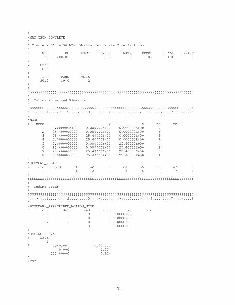
72

$ *MAT_CSCM_CONCRETE $ $ Concrete f'c = 30 MPa Maximum Aggregate Size is 19 mm $ $ MID RO NPLOT INCRE IRATE ERODE RECOV IRETRC 159 2.320E-09 1 0.0 0 1.05 0.0 0 $ $ PreD 0.0 $ $ f'c Dagg UNITS 30.0 19.0 2 $ $ $$$$$$$$$$$$$$$$$$$$$$$$$$$$$$$$$$$$$$$$$$$$$$$$$$$$$$$$$$$$$$$$$$$$$$$$$$$$$$$$ $ $ Define Nodes and Elements $ $$$$$$$$$$$$$$$$$$$$$$$$$$$$$$$$$$$$$$$$$$$$$$$$$$$$$$$$$$$$$$$$$$$$$$$$$$$$$$$$ $...>....1....>....2....>....3....>....4....>....5....>....6....>....7....>....8 $ *NODE $ node x y z tc rc 1 0.000000E+00 0.000000E+00 0.000000E+00 7 2 25.400000000 0.000000E+00 0.000000E+00 5 3 25.400000000 25.40000E+00 0.000000E+00 3 4 0.0000000000 25.40000E+00 0.000000E+00 6 5 0.0000000000 0.000000E+00 25.40000E+00 4 6 25.400000000 0.000000E+00 25.40000E+00 2 7 25.400000000 25.40000E+00 25.40000E+00 0 8 0.0000000000 25.40000E+00 25.40000E+00 1 $ *ELEMENT_SOLID $ eid pid n1 n2 n3 n4 n5 n6 n7 n8 1 1 1 2 3 4 5 6 7 8 $ $$$$$$$$$$$$$$$$$$$$$$$$$$$$$$$$$$$$$$$$$$$$$$$$$$$$$$$$$$$$$$$$$$$$$$$$$$$$$$$$ $ $ Define Loads $ $$$$$$$$$$$$$$$$$$$$$$$$$$$$$$$$$$$$$$$$$$$$$$$$$$$$$$$$$$$$$$$$$$$$$$$$$$$$$$$$ $...>....1....>....2....>....3....>....4....>....5....>....6....>....7....>....8 $ *BOUNDARY_PRESCRIBED_MOTION_NODE $ nid dof vad lcid sf vid 5 3 0 1 1.000E+00 6 3 0 1 1.000E+00 7 3 0 1 1.000E+00 8 3 0 1 1.000E+00 $ *DEFINE_CURVE $ lcid 1 $ abscissa ordinate 0.000 0.254 500.00000 0.254 $ *END

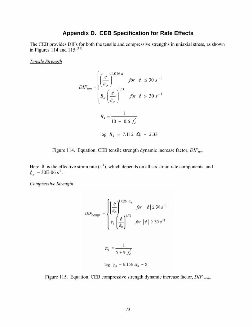
73

Appendix D. CEB Specification for Rate Effects

The CEB provides DIFs for both the tensile and compressive strengths in uniaxial stress, as shown in Figures 114 and 115:(11) Tensile Strength

Figure 114. Equation. CEB tensile strength dynamic increase factor, DIFten.

Here is the effective strain rate (s-1), which depends on all six strain rate components, and = 30E-06 s-1.

Compressive Strength

Figure 115. Equation. CEB compressive strength dynamic increase factor, DIFcomp.

⎪⎪

⎩

⎪⎪

⎨

⎧

>⎟⎟⎠

⎞⎜⎜⎝

⎛

≤⎟⎟⎠

⎞⎜⎜⎝

⎛

=−

−

13/1

1016.1

30

30

sforB

sfor DIF

os

d

oten

εεε

εεε

&&

&

&&

&

33.2112.7log

6.0101

'

−=

+=

ss

cs

B

fB

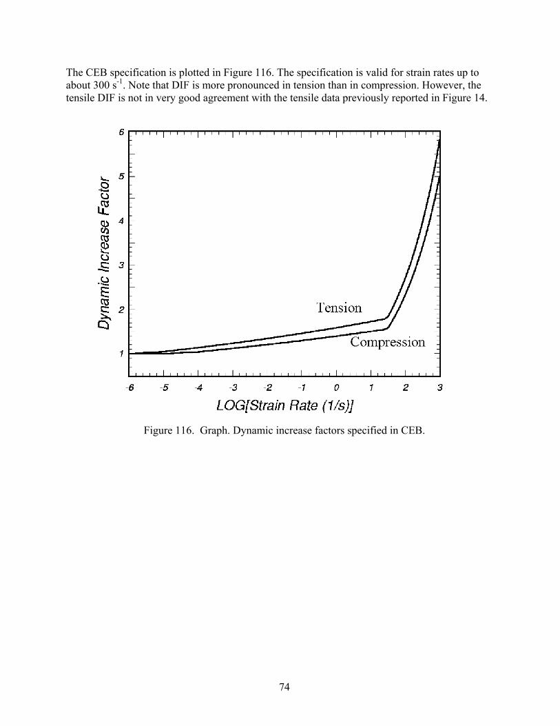
74

The CEB specification is plotted in Figure 116. The specification is valid for strain rates up to about 300 s-1. Note that DIF is more pronounced in tension than in compression. However, the tensile DIF is not in very good agreement with the tensile data previously reported in Figure 14.

Figure 116. Graph. Dynamic increase factors specified in CEB.

75

References

1. Murray, Y.D., A. Abu-Odeh, and R. Bligh, Evaluation of Concrete Material Model 159, FHWA-HRT-05-063, June 2006.

2. Murray, Y.D., Manual for LS-DYNA Wood Material Model 143, Report No. FHWA-HRT-04-

097, May 2006. 3. Murray, Y.D. and J. Reid, Evaluation of LS-DYNA Wood Material Model 143, Report No.

FHWA-HRT-04-096, August 2005. 4. Lewis, B.A., Manual for LS-DYNA Soil Material Model 147, Report No. FHWA-RD-04-095,

November 2004. 5. Lewis, B.A. and J. Reid, Evaluation of LS-DYNA Soil Material Model 147, Report No. FHWA-

RD-04-094, November 2004. 6. Livermore Software Technology Corporation, LS-DYNA Keyword Users Manual, Volumes 1

and 2, Version 970, 2003. 7. Chen, W.F. and D.J. Han, Plasticity for Structural Engineers, Springer-Verlag, New York,

1988. 8. Mills, L.L. and R.M. Zimmerman, “Compressive Strength of Plain Concrete Under Multiaxial

Loading Conditions,” ACI Journal 67(10), 1970, pp. 802–807. 9. Ottosen, N.S., “A Failure Criterion for Concrete,” Journal of Engineering Mechanics Division,

American Society for Civil Engineers (ASCE) 103 (EM4), 1977, pp. 527–535. 10. Launay, P., and H. Gachon, “Strain and Ultimate Strength of Concrete Under Triaxial Stress,”

Special Publication, SP-34, ACI 1, 1972, pp. 269–282.

11. CEB-FIP Model Code 1990, Comité Euro-International du Béton, Thomas Telford House, 1993.

12. Joy, S. and R. Moxley, White Sands Missile Range 5¾-inch Concrete Properties, United States

Army Engineers Waterways Experiment Station Briefing Prepared for Defense Special Weapons Agency, August 1993. Distribution limited to U.S. Government agencies and their contractors: critical technology.

13. Reinhardt, H.W., and H.A.W. Cornelissen, “Post-Peak Cyclic Behavior of Concrete in

Uniaxial and Alternating Tensile and Compressive Loading,” Cement and Concrete Research, Vol. 14, 1984, pp. 263–270.

76

14. Lee, Y., K. Willam, and H.D. Kang, “Experimental Observations of Concrete Behavior in Uniaxial Compression,” Fracture Mechanics of Concrete Structures, edited by F.H. Wittmann, July 1995.

15. Read, H.E., and C.J. Maiden, The Dynamic Behavior of Concrete, Systems, Science, and

Software Topical Report to Space and Missile Systems Organization, 3SR-707, August 1971. Defense Technical Information Center. U.S. Government Work (17 USC §015). Foreign copyrights may apply.

16. Kupfer, H., H. K. Hilsdorf, and H. Rusch, “Behavior of Concrete Under Biaxial Stress,” ACI

Journal, Title No. 66–52, August 1969, pp. 545–666. 17. Bischoff, P.H., and S.H. Perry, “Impact Behavior of Plain Concrete Loaded in Uniaxial

Compression,” Journal of Engineering Mechanics, June 1995, pp. 685–693. 18. Ross, C.A., and J.W. Tedesco, “Effects of Strain-Rate on Concrete Strength,” Presented at the

ACI 1991 Spring Convention, Washington, D.C., March 1992. 19. NCHRP Report 350, Recommended Procedures for the Safety Performance Evaluation of

Highway Features, Transportation Research Board, National Research Council. 20. Murray, Y.D., and B.A. Lewis, Numerical Simulation of Damage in Concrete, Technical report

submitted to the Defense Nuclear Agency by APTEK, Contract No. DNA001-94-C-0075, DNA-TR-95-190, November 1995.

21. Schwer, L.E. and Y.D. Murray, “A Three Invariant Smooth Cap Model with Mixed

Hardening,” International Journal for Numerical and Analytical Methods in Geomechanics, Vol. 18, pp. 657–688, 1994.

22. Pelessone, D., “A Modified Formulation of the Cap Model,” prepared by General Atomics for

DNA, GA-C19579, January 1989. 23. Sandler I, F.L. DiMaggio, and M.L. Barron, “An Extension of the Cap Model with Inclusion of

Pore Pressure Effects and Kinematic Hardening to Represent an Anisotropic Wet Clay,” in C.S. Desai and R.H. Gallagher Mechanics of Engineering Materials, Chapter 28, Wiley, New York, 1984.

24. Rubin, M.B., “Simple, Convenient Isotropic Failure Surface,” Journal of Engineering

Mechanics, Vol. 117, No. 2, February 1991, pp. 348–369. 25. Simo, J.C., J.W. Ju, “Strain and Stress Based Continuum Damage Model,” Int. J. of Solids and

Structures, Vol. 23, No. 7, 1987. 26. Simo, J.C., J.G. Kennedy, and S. Govindjee, “Non-Smooth Multisurface Plasticity and

Viscoplasticity. Loading/Unloading Conditions and Numerical Algorithms,” International Journal for Numerical Methods in Engineering, Vol. 26, 1988, pp. 2161–2185.

77

27. Murray Y.D., “Modeling Rate Effects in Rock and Concrete,” Proceedings of the 8th

International Symposium on Interaction of the Effects of Munitions with Structures, Volume IA, Defense Special Weapons Agency, McLean, VA, April 1997.

28. Attard, M.M. and S. Setunge, “Stress-Strain Relationship of Confined and Unconfined

Concrete,” ACI Materials Journal, September–October 1996, pp. 432–442. 29. Flatau, W.J., “Dynamic Tests of Large Reinforcing Bar Splices,” N-71-2, U.S. Army Engineer

Waterways Experiment Station, Vicksburg, MS, April 1971.

HRDS-04/05-07(1M)ERecycledRecyclable