User Guide v3
302
The Axon ™ Guide A guide to Electrophysiology and Biophysics Laboratory Techniques
-
Upload
adam-valdespino -
Category
Documents
-
view
221 -
download
0
Transcript of User Guide v3

8/13/2019 User Guide v3
http://slidepdf.com/reader/full/user-guide-v3 1/302
The Axon™ Guide
A guide to Electrophysiology andBiophysics Laboratory Techniques

8/13/2019 User Guide v3
http://slidepdf.com/reader/full/user-guide-v3 2/302
The Axon Guide
Electrophysiology and Biophysics LaboratoryTechniques
Third Edition
1-2500-0102 D
February 2012

8/13/2019 User Guide v3
http://slidepdf.com/reader/full/user-guide-v3 3/302
This document is provided to customers who have purchased Molecular Devices, LLC(“Molecular Devices”) equipment, software, reagents, and consumables to use in theoperation of such Molecular Devices equipment, software, reagents, andconsumables. This document is copyright protected and any reproduction of thisdocument, in whole or any part, is strictly prohibited, except as Molecular Devicesmay authorize in writing.
Software that may be described in this document is furnished under a licenseagreement. It is against the law to copy, modify, or distribute the software on anymedium, except as specifically allowed in the license agreement. Furthermore, thelicense agreement may prohibit the software from being disassembled, reverseengineered, or decompiled for any purpose.
Portions of this document may make reference to other manufacturers and/or theirproducts, which may contain parts whose names are registered as trademarks and/orfunction as trademarks of their respective owners. Any such usage is intended only
to designate those manufacturers’ products as supplied by Molecular Devices forincorporation into its equipment and does not imply any right and/or license to useor permit others to use such manufacturers’ and/or their product names astrademarks.
Molecular Devices makes no warranties or representations as to the fitness of thisequipment for any particular purpose and assumes no responsibility or contingentliability, including indirect or consequential damages, for any use to which thepurchaser may put the equipment described herein, or for any adverse circumstancesarising therefrom.
For research use only. Not for use in diagnostic procedures.
Product manufactured by Molecular Devices, LLC.
1311 Orleans Drive, Sunnyvale, California, United States of America 94089.
Molecular Devices, LLC is ISO 9001 registered.
© 2012 Molecular Devices, LLC.
All rights reserved.
The trademarks mentioned herein are the property of Molecular Devices, LLC or theirrespective owners. These trademarks may not be used in any type of promotion oradvertising without the prior written permission of Molecular Devices, LLC.
8/13/2019 User Guide v3
http://slidepdf.com/reader/full/user-guide-v3 4/302
1-2500-0102 D 3
Contents
Preface . . . . . . . . . . . . . . . . . . . . . . . . . . . . . . . . . . . . . . . 9
Introduction . . . . . . . . . . . . . . . . . . . . . . . . . . . . . . . . . . 11
Acknowledgment To Molecular Devices ConsultantsAnd Customers . . . . . . . . . . . . . . . . . . . . . . . . . . . . . . 11
Editorial . . . . . . . . . . . . . . . . . . . . . . . . . . . . . . . . . . . . . 13
Contributors . . . . . . . . . . . . . . . . . . . . . . . . . . . . . . . . . . 15
Chapter 1: Bioelectricity . . . . . . . . . . . . . . . . . . . . . . . . 17
Electrical Potentials . . . . . . . . . . . . . . . . . . . . . . . . . . . 17Electrical Currents . . . . . . . . . . . . . . . . . . . . . . . . . . . . 17
Resistors And Conductors . . . . . . . . . . . . . . . . . . . . . . . 19Ohm’s Law . . . . . . . . . . . . . . . . . . . . . . . . . . . . . . . . . 22The Voltage Divider . . . . . . . . . . . . . . . . . . . . . . . . . . . 24Perfect and Real Electrical Instruments. . . . . . . . . . . . . . 25Ions in Solutions and Electrodes . . . . . . . . . . . . . . . . . . 26Capacitors and Their Electrical Fields . . . . . . . . . . . . . . . 29Currents Through Capacitors. . . . . . . . . . . . . . . . . . . . . 31
Current Clamp and Voltage Clamp . . . . . . . . . . . . . . . . . 33Glass Microelectrodes and Tight Seals . . . . . . . . . . . . . . 34Further Reading. . . . . . . . . . . . . . . . . . . . . . . . . . . . . . 37
Chapter 2: The Laboratory Setup. . . . . . . . . . . . . . . . . . 39
The In Vitro Extracellular Recording Setup . . . . . . . . . . . 39The Single-channel Patch Clamping Setup . . . . . . . . . . . 39Vibration Isolation Methods. . . . . . . . . . . . . . . . . . . . . . 40
Electrical Isolation Methods. . . . . . . . . . . . . . . . . . . . . . 41Equipment Placement. . . . . . . . . . . . . . . . . . . . . . . . . . 43Further Reading. . . . . . . . . . . . . . . . . . . . . . . . . . . . . . 46

8/13/2019 User Guide v3
http://slidepdf.com/reader/full/user-guide-v3 5/302
Contents
4 1-2500-0102 D
Chapter 3: Instrumentation for Measuring BioelectricSignals from Cells . . . . . . . . . . . . . . . . . . . . . . . . . . . . . . 49
Extracellular Recording . . . . . . . . . . . . . . . . . . . . . . . . . 49Single-Cell Recording . . . . . . . . . . . . . . . . . . . . . . . . . . 50Multiple-cell Recording . . . . . . . . . . . . . . . . . . . . . . . . . 51Intracellular Recording Current Clamp. . . . . . . . . . . . . . . 51Intracellular Recording—Voltage Clamp. . . . . . . . . . . . . . 70Single-Channel Patch Clamp . . . . . . . . . . . . . . . . . . . . . 99Current Conventions and Voltage Conventions. . . . . . . . 110References . . . . . . . . . . . . . . . . . . . . . . . . . . . . . . . . 114
Chapter 4: Microelectrodes and Micropipettes. . . . . . . 117
Electrodes, Microelectrodes, Pipettes, Micropipettes,and Pipette Solutions . . . . . . . . . . . . . . . . . . . . . . . . . 117Fabrication of Patch Pipettes . . . . . . . . . . . . . . . . . . . . 119Pipette Properties for Single-channel vs.
Whole-Cell Recording . . . . . . . . . . . . . . . . . . . . . . . . . 121Types of Glasses and Their Properties. . . . . . . . . . . . . . 121Thermal Properties of Glasses . . . . . . . . . . . . . . . . . . . 124Noise Properties of Glasses . . . . . . . . . . . . . . . . . . . . . 125Leachable Components . . . . . . . . . . . . . . . . . . . . . . . . 127Further Reading . . . . . . . . . . . . . . . . . . . . . . . . . . . . . 127
Chapter 5: Advanced Methods in Electrophysiology . . 129
Recording from Xenopus Oocytes . . . . . . . . . . . . . . . . . 129Further Reading . . . . . . . . . . . . . . . . . . . . . . . . . . . . . 134Patch-Clamp Recording in Brain Slices . . . . . . . . . . . . . 135Further Reading . . . . . . . . . . . . . . . . . . . . . . . . . . . . . 142Macropatch and Loose-Patch Recording. . . . . . . . . . . . . 142The Giant Excised Membrane Patch Method . . . . . . . . . . 151Further Reading . . . . . . . . . . . . . . . . . . . . . . . . . . . . . 154
Recording from Perforated Patchesand Perforated Vesicles . . . . . . . . . . . . . . . . . . . . . . . . 154Further Reading . . . . . . . . . . . . . . . . . . . . . . . . . . . . . 163Enhanced Planar Bilayer Techniques forSingle-Channel Recording . . . . . . . . . . . . . . . . . . . . . . 164Further Reading . . . . . . . . . . . . . . . . . . . . . . . . . . . . . 177

8/13/2019 User Guide v3
http://slidepdf.com/reader/full/user-guide-v3 6/302
The Axon Guide to Electrophysiology and Biophysics Laboratory Techniques
1-2500-0102 D 5
Chapter 6: Signal Conditioning andSignal Conditioners . . . . . . . . . . . . . . . . . . . . . . . . . . . 179
Why Should Signals be Filtered? . . . . . . . . . . . . . . . . . 179Fundamentals of Filtering . . . . . . . . . . . . . . . . . . . . . . 180Filter Terminology . . . . . . . . . . . . . . . . . . . . . . . . . . . 182Preparing Signals for A/D Conversion . . . . . . . . . . . . . . 192Averaging . . . . . . . . . . . . . . . . . . . . . . . . . . . . . . . . . 200Line-frequency Pick-up (Hum). . . . . . . . . . . . . . . . . . . 200Peak-to-Peak and RMS Noise Measurements . . . . . . . . . 200Blanking . . . . . . . . . . . . . . . . . . . . . . . . . . . . . . . . . . 202Audio Monitor: Friend or Foe? . . . . . . . . . . . . . . . . . . . 202Electrode Test . . . . . . . . . . . . . . . . . . . . . . . . . . . . . . 203Common-Mode Rejection Ratio . . . . . . . . . . . . . . . . . . 203References . . . . . . . . . . . . . . . . . . . . . . . . . . . . . . . . 205Further Reading. . . . . . . . . . . . . . . . . . . . . . . . . . . . . 205
Chapter 7: Transducers . . . . . . . . . . . . . . . . . . . . . . . . 207Temperature Transducers for PhysiologicalTemperature Measurement . . . . . . . . . . . . . . . . . . . . . 207Temperature Transducers for ExtendedTemperature Ranges . . . . . . . . . . . . . . . . . . . . . . . . . 209Electrode Resistance and Cabling Affect Noiseand Bandwidth . . . . . . . . . . . . . . . . . . . . . . . . . . . . . 211
High Electrode Impedance Can ProduceSignal Attenuation . . . . . . . . . . . . . . . . . . . . . . . . . . . 211Unmatched Electrode Impedances IncreaseBackground Noise and Crosstalk . . . . . . . . . . . . . . . . . 213High Electrode Impedance Contributes to theThermal Noise of the System . . . . . . . . . . . . . . . . . . . 214Cable Capacitance Filters out the High-FrequencyComponent of the Signal . . . . . . . . . . . . . . . . . . . . . . 215EMG, EEG, EKG, and Neural Recording . . . . . . . . . . . . . 215Metal Microelectrodes. . . . . . . . . . . . . . . . . . . . . . . . . 216Bridge Design for Pressure and Force Measurements . . . 217Pressure Measurements . . . . . . . . . . . . . . . . . . . . . . . 218Force Measurements . . . . . . . . . . . . . . . . . . . . . . . . . 218Acceleration Measurements. . . . . . . . . . . . . . . . . . . . . 219Length Measurements . . . . . . . . . . . . . . . . . . . . . . . . 219

8/13/2019 User Guide v3
http://slidepdf.com/reader/full/user-guide-v3 7/302
Contents
6 1-2500-0102 D
Self-Heating Measurements . . . . . . . . . . . . . . . . . . . . . 219Isolation Measurements . . . . . . . . . . . . . . . . . . . . . . . 220Insulation Techniques . . . . . . . . . . . . . . . . . . . . . . . . . 220Further Reading . . . . . . . . . . . . . . . . . . . . . . . . . . . . . 220
Chapter 8: Laboratory Computer Issues andConsiderations . . . . . . . . . . . . . . . . . . . . . . . . . . . . . . . 223
Select the Software First . . . . . . . . . . . . . . . . . . . . . . . 223How Much Computer do you Need? . . . . . . . . . . . . . . . 223
Peripherals and Options . . . . . . . . . . . . . . . . . . . . . . . 224Recommended Computer Configurations . . . . . . . . . . . . 225Glossary . . . . . . . . . . . . . . . . . . . . . . . . . . . . . . . . . . 225
Chapter 9: Acquisition Hardware . . . . . . . . . . . . . . . . . 231
Fundamentals of Data Conversion . . . . . . . . . . . . . . . . 231Quantization Error . . . . . . . . . . . . . . . . . . . . . . . . . . . 233Choosing the Sampling Rate . . . . . . . . . . . . . . . . . . . . 234Converter Buzzwords . . . . . . . . . . . . . . . . . . . . . . . . . 235Deglitched DAC Outputs . . . . . . . . . . . . . . . . . . . . . . . 235Timers . . . . . . . . . . . . . . . . . . . . . . . . . . . . . . . . . . . 236Digital I/O . . . . . . . . . . . . . . . . . . . . . . . . . . . . . . . . . 237Optical Isolation . . . . . . . . . . . . . . . . . . . . . . . . . . . . . 237Operating Under Multi-Tasking Operating Systems. . . . . 238Software Support . . . . . . . . . . . . . . . . . . . . . . . . . . . . 238
Chapter 10: Data Analysis . . . . . . . . . . . . . . . . . . . . . . 239
Choosing Appropriate Acquisition Parameters . . . . . . . . 239Filtering at Analysis Time . . . . . . . . . . . . . . . . . . . . . . 241Integrals and Derivatives . . . . . . . . . . . . . . . . . . . . . . 242Single-Channel Analysis . . . . . . . . . . . . . . . . . . . . . . . 243Fitting . . . . . . . . . . . . . . . . . . . . . . . . . . . . . . . . . . . . 250
References . . . . . . . . . . . . . . . . . . . . . . . . . . . . . . . . 256

8/13/2019 User Guide v3
http://slidepdf.com/reader/full/user-guide-v3 8/302
The Axon Guide to Electrophysiology and Biophysics Laboratory Techniques
1-2500-0102 D 7
Chapter 11: Noise in ElectrophysiologicalMeasurements . . . . . . . . . . . . . . . . . . . . . . . . . . . . . . . 259
Thermal Noise . . . . . . . . . . . . . . . . . . . . . . . . . . . . . . 260Shot Noise . . . . . . . . . . . . . . . . . . . . . . . . . . . . . . . . 262Dielectric Noise . . . . . . . . . . . . . . . . . . . . . . . . . . . . . 263Excess Noise . . . . . . . . . . . . . . . . . . . . . . . . . . . . . . . 264Amplifier Noise . . . . . . . . . . . . . . . . . . . . . . . . . . . . . 265Electrode Noise . . . . . . . . . . . . . . . . . . . . . . . . . . . . . 268Seal Noise. . . . . . . . . . . . . . . . . . . . . . . . . . . . . . . . . 278Noise in Whole-cell Voltage Clamping. . . . . . . . . . . . . . 279External Noise Sources. . . . . . . . . . . . . . . . . . . . . . . . 282Digitization Noise. . . . . . . . . . . . . . . . . . . . . . . . . . . . 283Aliasing . . . . . . . . . . . . . . . . . . . . . . . . . . . . . . . . . . 284Filtering . . . . . . . . . . . . . . . . . . . . . . . . . . . . . . . . . . 287Summary of Patch-Clamp Noise. . . . . . . . . . . . . . . . . . 291Limits of Patch-Clamp Noise Performance . . . . . . . . . . . 293
Further Reading. . . . . . . . . . . . . . . . . . . . . . . . . . . . . 293
Appendix A: Guide to Interpreting Specifications . . . . 295
General . . . . . . . . . . . . . . . . . . . . . . . . . . . . . . . . . . 295RMS Versus Peak-to-Peak Noise . . . . . . . . . . . . . . . . . 296Bandwidth—Time Constant—Rise Time. . . . . . . . . . . . . 296Filters. . . . . . . . . . . . . . . . . . . . . . . . . . . . . . . . . . . . 296
Microelectrode Amplifiers . . . . . . . . . . . . . . . . . . . . . . 297Patch-Clamp Amplifiers. . . . . . . . . . . . . . . . . . . . . . . . 298

8/13/2019 User Guide v3
http://slidepdf.com/reader/full/user-guide-v3 9/302
Contents
8 1-2500-0102 D

8/13/2019 User Guide v3
http://slidepdf.com/reader/full/user-guide-v3 10/302
1-2500-0102 D 9
Preface
Molecular Devices is pleased to present you with the third edition of theAxon Guide, a laboratory guide to electrophysiology and biophysics.The purpose of this guide is to serve as an information and dataresource for electrophysiologists. It covers a broad scope of topicsranging from the biological basis of bioelectricity and a description ofthe basic experimental setup to a discussion of mechanisms of noise
and data analysis.The Axon Guide third edition is a tool benefiting both the novice and theexpert electrophysiologist. Newcomers to electrophysiology will gain anappreciation of the intricacies of electrophysiological measurementsand the requirements for setting up a complete recording and analysissystem. For experienced electrophysiologists, we include in-depthdiscussions of selected topics, such as advanced methods inelectrophysiology and noise.
This edition is the first major revision of the Axon Guide since the
original edition was published in 1993. While the fundamentals ofelectrophysiology have not changed in that time, changes ininstrumentation and computer technology made a number of theoriginal chapters interesting historical documents rather than helpfulguides. This third edition is up-to-date with current developments intechnology and instrumentation.
This guide was the product of a collaborative effort of many researchersin the field of electrophysiology and the staff of Molecular Devices. Weare deeply grateful to these individuals for sharing their knowledge and
devoting significant time and effort to this endeavor.
David Yamane
Director, Electrophysiology Marketing
Molecular Devices

8/13/2019 User Guide v3
http://slidepdf.com/reader/full/user-guide-v3 11/302
Preface
10 1-2500-0102 D
8/13/2019 User Guide v3
http://slidepdf.com/reader/full/user-guide-v3 12/302
1-2500-0102 D 11
Introduction
Axon Instruments, Inc. was founded in 1983 to design andmanufacture instrumentation and software for electrophysiology andbiophysics. Its products were distinguished by the company’sinnovative design capability, high-quality products, and expert technicalsupport. Today, the Axon Instruments products are part of theMolecular Devices portfolio of life science and drug discovery products.
The Axon brand of microelectrode amplifiers, digitizers, and dataacquisition and analysis software provides researchers withready-to-use, technologically advanced products which allows themmore time to pursue their primary research goals.
Furthermore, to ensure continued success with our products, we havestaffed our Technical Support group with experienced Ph.D.electrophysiologists.
In addition to the Axon product suite, Molecular Devices has developedthree automated electrophysiology platforms. Together with the Axon
Conventional Electrophysiology products, Molecular Devices spans theentire drug discovery process from screening to safety assessment.
In recognition of the continuing excitement in ion channel research, asevidenced by the influx of molecular biologists, biochemists, andpharmacologists into this field, Molecular Devices is proud to supportthe pursuit of electrophysiological and biophysical research with thislaboratory techniques workbook.
Acknowledgment To Molecular Devices ConsultantsAnd Customers
Molecular Devices employs a talented team of engineers and scientistsdedicated to designing instruments and software incorporating themost advanced technology and the highest quality. Nevertheless, itwould not be possible for us to enhance our products without closecollaborations with members of the scientific community. Thesecollaborations take many forms.
Some scientists assist Molecular Devices on a regular basis, sharingtheir insights on current needs and future directions of scientificresearch. Others assist us by virtue of a direct collaboration in thedesign of certain products. Many scientists help us by reviewing ourinstrument designs and the development versions of various softwareproducts. We are grateful to these scientists for their assistance. Wealso receive a significant number of excellent suggestions from thecustomers we meet at scientific conferences. To all of you who havevisited us at our booths and shared your thoughts, we extend our

8/13/2019 User Guide v3
http://slidepdf.com/reader/full/user-guide-v3 13/302
Introduction
12 1-2500-0102 D
sincere thanks. Another source of feedback for us is the informationthat we receive from the conveners of the many excellent summer
courses and workshops that we support with equipment loans. Ourgratitude is extended to them for the written assessments they oftensend us outlining the strengths and weaknesses of Axon ConventionalElectrophysiology products from Molecular Devices.

8/13/2019 User Guide v3
http://slidepdf.com/reader/full/user-guide-v3 14/302
1-2500-0102 D 13
Editorial
Editor
Rivka Sherman-Gold, Ph.D.
Editorial Committee
Michael J. Delay, Ph.D.
Alan S. Finkel, Ph.D.
Henry A. Lester, Ph.D.1
W. Geoffrey Powell, MBA
Rivka Sherman-Gold, Ph.D.
Layout and Editorial Assistance
Jay Kurtz
ArtworkElizabeth Brzeski
Editor – 3rd Edition
Warburton H. Maertz
Editorial Committee – 3rd Edition
Scott V. Adams, Ph.D.
S. Clare Chung, Ph.D.
Toni Figl, Ph.D.
Warburton H. Maertz
Damian J. Verdnik, Ph.D.
Layout and Editorial Assistance – 3rd Edition
Simone Andrews
Eveline Pajares
Peter Valenzuela
Damian J. Verdnik, Ph.D.
Alfred Walter, Ph.D.

8/13/2019 User Guide v3
http://slidepdf.com/reader/full/user-guide-v3 15/302
Editorial
14 1-2500-0102 D
Acknowledgements
The valuable inputs and insightful comments of Dr. Bertil Hille, Dr. JoeImmel, and Dr. Stephen Redman are much appreciated.

8/13/2019 User Guide v3
http://slidepdf.com/reader/full/user-guide-v3 16/302
1-2500-0102 D 15
Contributors
The Axon Guide is the product of a collaborative effort of MolecularDevices and researchers from several institutions whose contributionsto the guide are gratefully acknowledged.
John M. Bekkers, Ph.D., Division of Neuroscience, John Curtin School ofMedical Research, Australian National University, Canberra, A.C.T.Australia.
Richard J. Bookman, Ph.D., Department of Molecular & CellularPharmacology, Miller School of Medicine, University of Miami, Miami,Florida.
Michael J. Delay, Ph.D.
Alan S. Finkel, Ph.D.
Aaron Fox, Ph.D., Department of Neurobiology, Pharmacology andPhysiology, University of Chicago, Chicago, Illinois.
David Gallegos.Robert I. Griffiths, Ph.D., Monash Institute of Medical Research, Facultyof Medicine, Monash University, Clayton, Victoria, Australia.
Donald Hilgemann, Ph.D., Graduate School of Biomedical Sciences,Southwestern Medical School, Dallas, Texas.
Richard H. Kramer, Department of Molecular & Cell Biology, Universityof California Berkeley, Berkeley, California.
Henry A. Lester, Ph.D., Division of Biology, California Institute of
Technology, Pasadena, California.Richard A. Levis, Ph.D., Department of Molecular Biophysics &Physiology, Rush-Presbyterian-St. Luke’s Medical College, Chicago,Illinois.
Edwin S. Levitan, Ph.D., Department of Pharmacology, School ofMedicine, University of Pittsburgh, Pittsburgh, Pennsylvania.
M. Craig McKay, Ph.D., Department of Molecular Endocrinology,GlaxoSmithKline, Inc., Research Triangle Park, North Carolina.
David J. Perkel, Department of Biology, University of Washington,Seattle, Washington.
Stuart H. Thompson, Hopkins Marine Station, Stanford University,Pacific Grove, California.
James L. Rae, Ph.D., Department of Physiology and BiomedicalEngineering, Mayo Clinic, Rochester, Minnesota.
Michael M. White, Ph.D., Department of Pharmacology & Physiology,Drexel University College of Medicine, Philadelphia, Pennsylvania.

8/13/2019 User Guide v3
http://slidepdf.com/reader/full/user-guide-v3 17/302
Contributors
16 1-2500-0102 D
William F. Wonderlin, Ph.D., Department of Biochemistry & MolecularPhamacology, West Virginia University, Morgantown, West Virginia.

8/13/2019 User Guide v3
http://slidepdf.com/reader/full/user-guide-v3 18/302
1-2500-0102 D 17
1Bioelectricity
Chapter 1 introduces the basic concepts used in making electricalmeasurements from cells and the techniques used to make thesemeasurements.
Electrical Potentials
A cell derives its electrical properties mostly from the electricalproperties of its membrane. A membrane, in turn, acquires itsproperties from its lipids and proteins, such as ion channels andtransporters. An electrical potential difference exists between theinterior and exterior of cells. A charged object (ion) gains or losesenergy as it moves between places of different electrical potential, justas an object with mass moves “up” or “down” between points ofdifferent gravitational potential. Electrical potential differences areusually denoted as V or ΔV and measured in volts. Potential is alsotermed voltage. The potential difference across a cell relates thepotential of the cell’s interior to that of the external solution, which,according to the commonly accepted convention, is zero.
The potential difference across a lipid cellular membrane(“transmembrane potential”) is generated by the “pump” proteins thatharness chemical energy to move ions across the cell membrane. Thisseparation of charge creates the transmembrane potential. Because thelipid membrane is a good insulator, the transmembrane potential ismaintained in the absence of open pores or channels that can conductions.
Typical transmembrane potentials amount to less than 0.1 V, usually 30to 90 mV in most animal cells, but can be as much as 200 mV in plantcells. Because the salt-rich solutions of the cytoplasm and extracellularmilieu are fairly good conductors, there are usually very smalldifferences at steady state (rarely more than a few millivolts) betweenany two points within a cell’s cytoplasm or within the extracellularsolution. Electrophysiological equipment enables researchers tomeasure potential (voltage) differences in biological systems.
Electrical Currents
Electrophysiological equipment can also measure current, which is theflow of electrical charge passing a point per unit of time. Current (I) ismeasured in amperes (A). Usually, currents measured byelectrophysiological equipment range from picoamperes tomicroamperes. For instance, typically, 104 Na+ ions cross the
membrane each millisecond that a single Na+
channel is open. This

8/13/2019 User Guide v3
http://slidepdf.com/reader/full/user-guide-v3 19/302
Bioelectricity
18 1-2500-0102 D
current equals 1.6 pA (1.6 x 10⁻¹⁹ C/ion x 104 ions/ms x 103 ms/s; recallthat 1 A is equal to 1 coulomb (C)/s).
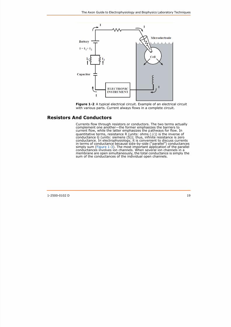
Two handy rules about currents often help to understandelectrophysiological phenomena: 1) current is conserved at a branchpoint (Figure 1-1); and 2) current always flows in a complete circuit(Figure 1-2). In electrophysiological measurements, currents can flowthrough capacitors, resistors, ion channels, amplifiers, electrodes andother entities, but they always flow in complete circuits.
Figure 1-1 Conservation of current. Current is conserved at a branchpoint.
8/13/2019 User Guide v3
http://slidepdf.com/reader/full/user-guide-v3 20/302
The Axon Guide to Electrophysiology and Biophysics Laboratory Techniques
1-2500-0102 D 19
Figure 1-2 A typical electrical circuit. Example of an electrical circuitwith various parts. Current always flows in a complete circuit.
Resistors And Conductors
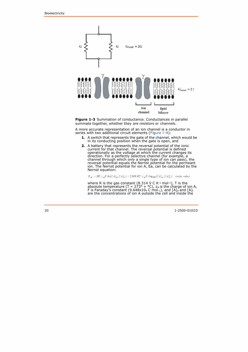
Currents flow through resistors or conductors. The two terms actuallycomplement one another—the former emphasizes the barriers tocurrent flow, while the latter emphasizes the pathways for flow. Inquantitative terms, resistance R (units: ohms (Ω)) is the inverse ofconductance G (units: siemens (S)); thus, infinite resistance is zeroconductance. In electrophysiology, it is convenient to discuss currentsin terms of conductance because side-by-side (“parallel”) conductancessimply sum (Figure 1-3). The most important application of the parallelconductances involves ion channels. When several ion channels in amembrane are open simultaneously, the total conductance is simply thesum of the conductances of the individual open channels.
8/13/2019 User Guide v3
http://slidepdf.com/reader/full/user-guide-v3 21/302
Bioelectricity
20 1-2500-0102 D
Figure 1-3 Summation of conductance. Conductances in parallelsummate together, whether they are resistors or channels.
A more accurate representation of an ion channel is a conductor inseries with two additional circuit elements (Figure 1-4):
1. A switch that represents the gate of the channel, which would bein its conducting position when the gate is open, and
2. A battery that represents the reversal potential of the ioniccurrent for that channel. The reversal potential is definedoperationally as the voltage at which the current changes itsdirection. For a perfectly selective channel (for example, achannel through which only a single type of ion can pass), the
reversal potential equals the Nernst potential for the permeantion. The Nernst potential for ion A, Ea, can be calculated by theNernst equation:
where R is the gas constant (8.314 V C K-1 mol-1), T is theabsolute temperature (T = 273° + °C), zA is the charge of ion A,F is Faraday’s constant (9.648x10⁴ C mol-1), and [A]o and [A]i
are the concentrations of ion A outside the cell and inside the

8/13/2019 User Guide v3
http://slidepdf.com/reader/full/user-guide-v3 22/302

8/13/2019 User Guide v3
http://slidepdf.com/reader/full/user-guide-v3 23/302
Bioelectricity
22 1-2500-0102 D
potential for that ion. Since a typical cell membrane at rest has a muchhigher permeability to potassium (PK) than to sodium, calcium or
chloride (PNa, PCa and PCl, respectively), the resting membrane potentialis very close to EK, the potassium reversal potential.
Ohm’s Law
For electrophysiology, perhaps the most important law of electricity isOhm’s law. The potential difference between two points linked by acurrent path with a conductance G and a current I (Figure 1-5) is:
Figure 1-5 Figure 1.5: Ohm’s law.
This concept applies to any electrophysiological measurement, asillustrated by the two following examples:
1. In an extracellular recording experiment: the current I thatflows between parts of a cell through the external resistance Rproduces a potential difference ΔV, which is usually less than 1
mV (Figure 1-6). As the impulse propagates, I changes and,therefore, ΔV changes as well.
Th A G id t El t h i l d Bi h i L b t T h i

8/13/2019 User Guide v3
http://slidepdf.com/reader/full/user-guide-v3 24/302
The Axon Guide to Electrophysiology and Biophysics Laboratory Techniques
1-2500-0102 D 23
Figure 1-6 IR drop. In extracellular recording, current I thatflows between points of a cell is measured as the potentialdifference (“IR drop”) across the resistance R of the fluidbetween the two electrodes.
2. In a voltage-clamp experiment: when N channels, each ofconductance γ, are open, the total conductance is Nγ. Theelectrochemical driving force ΔV (membrane potential minus
reversal potential) produces a current NγΔV. As channels openand close, N changes and so does the voltage-clamp current I.Hence, the voltage-clamp current is simply proportional to thenumber of open channels at any given time. Each channel canbe considered as a γ conductance increment.
Bioelectricity

8/13/2019 User Guide v3
http://slidepdf.com/reader/full/user-guide-v3 25/302
Bioelectricity
24 1-2500-0102 D
The Voltage Divider
Figure 1-7 describes a simple circuit called a voltage divider in whichtwo resistors are connected in series:
Figure 1-7 A voltage divider.
The total potential difference provided by the battery is E; a portion ofthis voltage appears across each resistor:
When two resistors are connected in series, the same current passes
through each of them. Therefore the circuit is described by:
where E is the value of the battery, which equals the total potentialdifference across both resistors. As a result, the potential difference isdivided in proportion to the two resistance values.
The Axon Guide to Electrophysiology and Biophysics Laboratory Techniques

8/13/2019 User Guide v3
http://slidepdf.com/reader/full/user-guide-v3 26/302
The Axon Guide to Electrophysiology and Biophysics Laboratory Techniques
1-2500-0102 D 25
Perfect and Real Electrical Instruments
Electrophysiological measurements should satisfy two requirements: 1)They should accurately measure the parameter of interest, and 2) theyshould produce no perturbation of the parameter. The first requirementcan be discussed in terms of a voltage divider. The second point will bediscussed after addressing electrodes.
The best way to measure an electrical potential difference is to use avoltmeter with infinite resistance. To illustrate this point, consider thearrangement of Figure 1-8 A, which can be reduced to the equivalentcircuit of Figure 1-8 B.
Figure 1-8 Representative voltmeter with infinite resistance.Instruments used to measure potentials must have a very high inputresistance Rin.
Bioelectricity

8/13/2019 User Guide v3
http://slidepdf.com/reader/full/user-guide-v3 27/302
Bioelectricity
26 1-2500-0102 D
Before making the measurement, the cell has a resting potential of Erp,which is to be measured with an intracellular electrode of resistance Re.To understand the effect of the measuring circuit on the measuredparameter, we will pretend that our instrument is a “perfect” voltmeter(for example, with an infinite resistance) in parallel with a finiteresistance Rin, which represents the resistance of a real voltmeter orthe measuring circuit. The combination Re and Rin forms a voltagedivider, so that only a fraction of Erp appears at the input of the “perfect” voltmeter; this fraction equals ErpRin /(Rin + Re). The larger Rin,the closer V is to Erp. Clearly the problem gets more serious as theelectrode resistance Re increases, but the best solution is to make Rin aslarge as possible.
On the other hand, the best way to measure current is to open the pathand insert an ammeter. If the ammeter has zero resistance, it will notperturb the circuit since there is no IR-drop across it.
Ions in Solutions and Electrodes
Ohm’s law—the linear relation between potential difference and currentflow—applies to aqueous ionic solutions, such as blood, cytoplasm, and
sea water. Complications are introduced by two factors:1. The current is carried by at least two types of ions (one anion
and one cation) and often by many more. For each ion, currentflow in the bulk solution is proportional to the potentialdifference. For a first approximation, the conductance of thewhole solution is simply the sum of the conductancescontributed by each ionic species. When the current flowsthrough ion channels, it is carried selectively by only a subset ofthe ions in the solution.
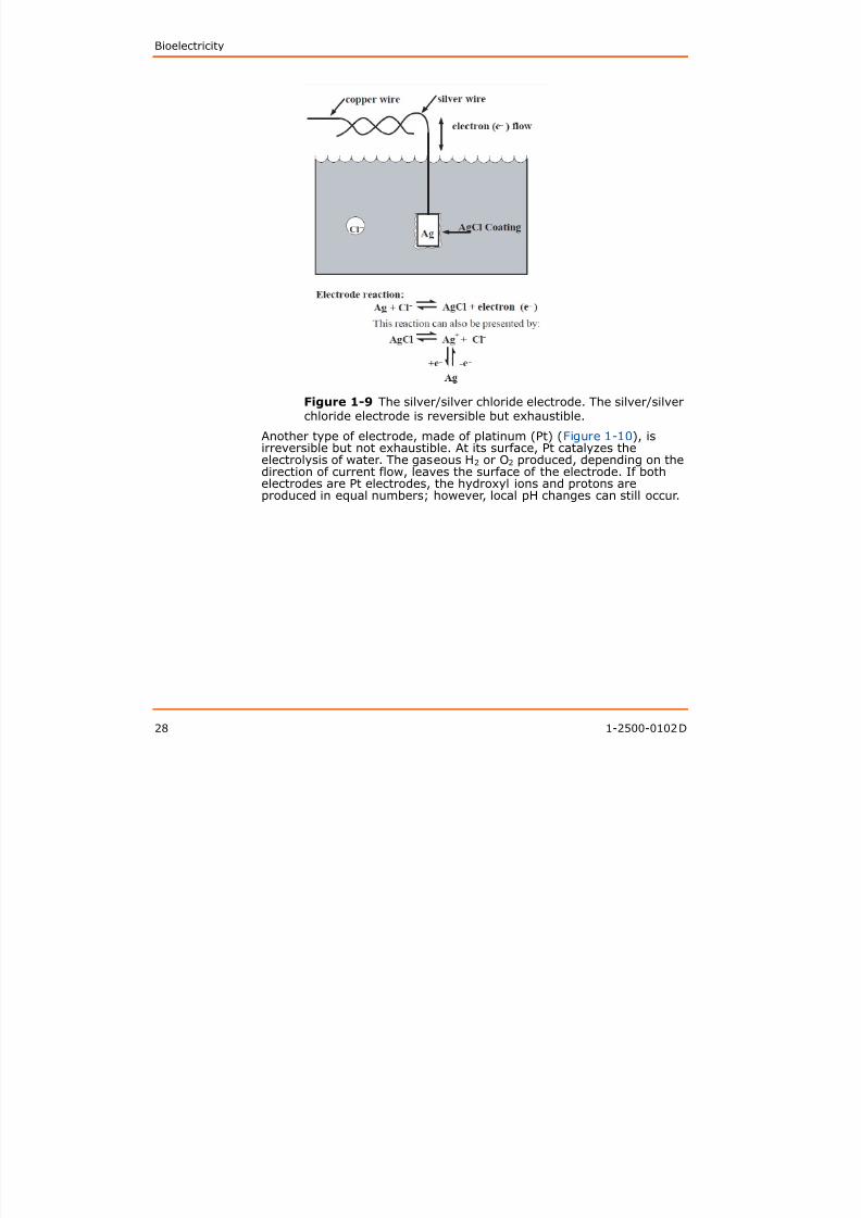
2. At the electrodes, current must be transformed smoothly from aflow of electrons in the copper wire to a flow of ions in solution.Many sources of errors (artifacts) are possible. Several types ofelectrodes are used in electrophysiological measurements. Themost common is a silver/silver chloride (Ag/AgCl) interface,which is a silver wire coated with silver chloride (Figure 1-9). Ifelectrons flow from the copper wire through the silver wire tothe electrode AgCl pellet, they convert the AgCl to Ag atoms andthe Cl- ions become hydrated and enter the solution. If electrons
flow in the reverse direction, Ag atoms in the silver wire that iscoated with AgCl give up their electrons (one electron per atom)and combine with Cl- ions that are in the solution to makeinsoluble AgCl. This is, therefore, a reversible electrode, forexample, current can flow in both directions.
The Axon Guide to Electrophysiology and Biophysics Laboratory Techniques
8/13/2019 User Guide v3
http://slidepdf.com/reader/full/user-guide-v3 28/302
p y gy p y y q
1-2500-0102 D 27
There are several points to remember about Ag/AgCl electrodes:
The Ag/AgCl electrode performs well only in solutions
containing chloride ions. Because current must flow in a complete circuit, two
electrodes are needed. If the two electrodes face different Cl- concentrations (for instance, 3 M KCl inside a micropipette1 and 120 mM NaCl in a bathing solution surrounding the cell),there will be a difference in the half-cell potentials (thepotential difference between the solution and the electrode)at the two electrodes, resulting in a large steady potentialdifference in the two wires attached to the electrodes. This
steady potential difference, termed liquid junction potential,can be subtracted electronically and poses few problems aslong as the electrode is used within its reversible limits.
If the AgCl is exhausted by the current flow, bare silver couldcome in contact with the solution. Silver ions leaking fromthe wire can poison many proteins. Also, the half-cellpotentials now become dominated by unpredictable, poorlyreversible surface reactions due to other ions in the solutionand trace impurities in the silver, causing electrodepolarization. However, used properly, Ag/AgCl electrodespossess the advantages of little polarization and predictable junction potential.
1. A micropipette is a pulled capillary glass into which the Ag/AgC1 electrode is
inserted (see Chapter 4: Microelectrodes and Micropipettes on page 117).
Bioelectricity
8/13/2019 User Guide v3
http://slidepdf.com/reader/full/user-guide-v3 29/302
28 1-2500-0102 D
Figure 1-9 The silver/silver chloride electrode. The silver/silverchloride electrode is reversible but exhaustible.
Another type of electrode, made of platinum (Pt) (Figure 1-10), isirreversible but not exhaustible. At its surface, Pt catalyzes theelectrolysis of water. The gaseous H2 or O2 produced, depending on thedirection of current flow, leaves the surface of the electrode. If bothelectrodes are Pt electrodes, the hydroxyl ions and protons areproduced in equal numbers; however, local pH changes can still occur.
The Axon Guide to Electrophysiology and Biophysics Laboratory Techniques

8/13/2019 User Guide v3
http://slidepdf.com/reader/full/user-guide-v3 30/302
1-2500-0102 D 29
Figure 1-10 The platinum electrode. A platinum electrode is
irreversible but inexhaustible.
Capacitors and Their Electrical Fields
The electrical field is a property of each point in space and is defined asproportional to the force experienced by a charge placed at that point.The greater the potential difference between two points fixed in space,the greater the field at each point between them. Formally, the
electrical field is a vector defined as the negative of the spatialderivative of the potential.
The concept of the electrical field is important for understandingmembrane function. Biological membranes are typically less than10 nm thick. Consequently, a transmembrane resting potential of about100 mV produces a very sizable electrical field in the membrane ofabout 105 V/cm. This is close to the value at which most insulatorsbreak down irreversibly because their atoms become ionized. Ofcourse, typical electrophysiological equipment cannot measure these
fields directly. However, changes in these fields are presumably sensedby the gating domains of voltage-sensitive ion channels, whichdetermine the opening and closing of channels, and so the electricalfields underlie the electrical excitability of membranes.
Bioelectricity

8/13/2019 User Guide v3
http://slidepdf.com/reader/full/user-guide-v3 31/302
30 1-2500-0102 D
Another consequence of the membrane’s thinness is that it makes anexcellent capacitor. Capacitance (C; measured in farads, F) is the ability
to store charge Q when a voltageΔ
V occurs across the two “ends,” sothat:
The formal symbol for a capacitor is two parallel lines (Figure 1-12).This symbol arose because the most effective capacitors are parallelconducting plates of large area separated by a thin sheet of insulator(Figure 1-11) an excellent approximation of the lipid bilayer.
The capacitance C is proportional to the area and inversely proportional
to the distance separating the two conducting sheets.
Figure 1-11 Capacitance. A charge Q is stored in a capacitor of value
C held at a potential ΔV.
When multiple capacitors are connected in parallel, this is electronicallyequivalent to a single large capacitor; that is, the total capacitance isthe sum of their individual capacitance values (Figure 1-12). Thus,
membrane capacitance increases with cell size. Membrane capacitanceis usually expressed as value per unit area; nearly all lipid bilayermembranes of cells have a capacitance of 1 μF/cm2 (0.01 pF/μm2).
The Axon Guide to Electrophysiology and Biophysics Laboratory Techniques

8/13/2019 User Guide v3
http://slidepdf.com/reader/full/user-guide-v3 32/302
1-2500-0102 D 31
Figure 1-12 Capacitors in parallel add their values.
Currents Through CapacitorsThe following equation shows that charge is stored in a capacitor onlywhen there is a change in the voltage across the capacitor. Therefore,the current flowing through capacitance C is proportional to the voltagechange with time:
Until now, we have been discussing circuits whose properties do notchange with time. As long as the voltage across a membrane remainsconstant, one can ignore the effect of the membrane capacitance onthe currents flowing across the membrane through ion channels. Whilethe voltage changes, there are transient capacitive currents in additionto the steady-state currents through conductive channels. Thesecapacitive currents constitute one of the two major influences on thetime-dependent electrical properties of cells (the other is the kinetics ofchannel gating). On Axon Conventional Electrophysiology
voltage-clamp or patch-clamp amplifiers, several controls are devotedto handle these capacitive currents. Therefore it is worth obtainingsome intuitive “feel” for their behavior.
The stored charge on the membrane capacitance accompanies theresting potential, and any change in the voltage across the membraneis accompanied by a change in this stored charge. Indeed, if a currentis applied to the membrane, either by channels elsewhere in the cell orby current from the electrode, this current first satisfies therequirement for charging the membrane capacitance, then it changes
Bioelectricity

8/13/2019 User Guide v3
http://slidepdf.com/reader/full/user-guide-v3 33/302
32 1-2500-0102 D
the membrane voltage. Formally, this can be shown by representing themembrane as a resistor of value R in parallel with capacitance C(Figure 1-13).
Figure 1-13 Membrane behavior compared with an electrical current.A membrane behaves electrically like a capacitance in parallel with aresistance.
Now, if we apply a pulse of current to the circuit, the current firstcharges up the capacitance, then changes the voltage (Figure 1-14).
Figure 1-14 RC parallel circuit response. Response of an RC parallelcircuit to a step of current.
The Axon Guide to Electrophysiology and Biophysics Laboratory Techniques

8/13/2019 User Guide v3
http://slidepdf.com/reader/full/user-guide-v3 34/302
1-2500-0102 D 33
The voltage V(t) approaches steady state along an exponential timecourse:
The steady-state value Vinƒ (also called the infinite-time or equilibriumvalue) does not depend on the capacitance; it is simply determined bythe current I and the membrane resistance R:
This is just Ohm’s law, of course; but when the membrane capacitanceis in the circuit, the voltage is not reached immediately. Instead, it isapproached with the time constant τ, given by:
Thus, the charging time constant increases when either the membranecapacitance or the resistance increases. Consequently, large cells, suchas Xenopus oocytes that are frequently used for expression of genesencoding ion-channel proteins, and cells with extensive membrane
invigorations, such as the T-system in skeletal muscle, have a longcharging phase.
Current Clamp and Voltage Clamp
In a current-clamp experiment, one applies a known constant or time-varying current and measures the change in membrane potentialcaused by the applied current. This type of experiment mimics thecurrent produced by a synaptic input.
In a voltage clamp experiment one controls the membrane voltage andmeasures the transmembrane current required to maintain thatvoltage. Despite the fact that voltage clamp does not mimic a processfound in nature, there are three reasons to do such an experiment:
1. Clamping the voltage eliminates the capacitive current, exceptfor a brief time following a step to a new voltage (Figure 1-15).The brevity of the capacitive current depends on many factorsthat are discussed in following chapters.
2. Except for the brief charging time, the currents that flow areproportional only to the membrane conductance, for example,to the number of open channels.
3. If channel gating is determined by the transmembrane voltagealone (and is insensitive to other parameters such as the currentand the history of the voltage), voltage clamp offers control overthe key variable that determines the opening and closing of ionchannels.
Bioelectricity

8/13/2019 User Guide v3
http://slidepdf.com/reader/full/user-guide-v3 35/302
34 1-2500-0102 D
Figure 1-15 Typical voltage-clamp experiment. Avoltage-clamp experiment on the circuit of Figure 1-13.
The patch clamp is a special voltage clamp that allows one to resolvecurrents flowing through single ion channels. It also simplified themeasurement of currents flowing through the whole-cell membrane,particularly in small cells that cannot be easily penetrated withelectrodes. The characteristics of a patch clamp are dictated by twofacts:
1. The currents measured are very small, on the order ofpicoamperes in single-channel recording and usually up toseveral nanoamperes in whole-cell recording. Due to the smallcurrents, particularly in single-channel recording, the electrodepolarizations and nonlinearities are negligible and the Ag/AgClelectrode can record voltage accurately even while passingcurrent.
2. The electronic ammeter must be carefully designed to avoidadding appreciable noise to the currents it measures.
Glass Microelectrodes and Tight Seals
Successful electrophysiological measurements depend on twotechnologies: the design of electronic instrumentation and theproperties and fabrication of glass micropipettes. Glass pipettes areused both for intracellular recording and for patch recording; quartzpipettes have been used for ultra low-noise single-channel recording
The Axon Guide to Electrophysiology and Biophysics Laboratory Techniques

8/13/2019 User Guide v3
http://slidepdf.com/reader/full/user-guide-v3 36/302
1-2500-0102 D 35
(for a detailed discussion of electrode glasses see Chapter 4:Microelectrodes and Micropipettes on page 117). Successful patchrecording requires a tight seal between the pipette and the membrane.Although there is not yet a satisfactory molecular description of thisseal, we can describe its electrical characteristics.
Requirement 2) above (see Perfect and Real Electrical Instruments onpage 25) states that the quality of the measurement depends onminimizing perturbation of the cells. For the case of voltage recording,this point can be presented with the voltage divider circuit (Figure 1-16).
Figure 1-16 Intracellular electrode measurement. This intracellularelectrode is measuring the resting potential of a cell whose membranecontains only open K+ channels. As the seal resistance Rs increases,the measurement approaches the value of EK.
For the case of patch recording, currents through the seal do not distort
the measured voltage or current, but they do add to the current noise.Current noise can be analyzed either in terms of the Johnson noise of aconductor, which is the thermal noise that increases with theconductance (see Chapter 7: Transducers on page 207 and Chapter 11:Noise in Electrophysiological Measurements on page 259), or in termsof simple statistics. The latter goes as follows: If a current of N ions/mspasses through an open channel, then the current will fluctuate fromone millisecond to the next with a standard deviation of √ N. Thesefluctuations produce noise on the single-channel recorded traces. If anadditional current is flowing in parallel through the seal (Figure 1-17), it
causes an increase in the standard deviations. For instance, if thecurrent through the seal is ten-fold larger than through the channel,then the statistical fluctuations in current flow produced by the seal are√ 10 (316%) larger than they would be for a “perfect” seal.
Bioelectricity

8/13/2019 User Guide v3
http://slidepdf.com/reader/full/user-guide-v3 37/302
36 1-2500-0102 D
Figure 1-17 Good and bad seals. In a patch recording, currentsthrough the seal also flow through the measuring circuit, increasing thenoise on the measured current.
The Axon Guide to Electrophysiology and Biophysics Laboratory Techniques

8/13/2019 User Guide v3
http://slidepdf.com/reader/full/user-guide-v3 38/302
1-2500-0102 D 37
Further Reading
Brown, K. T., Flaming, D. G. Advanced Micropipette Techniques for CellPhysiology. John Wiley & Sons, New York, NY, 1986.
Hille, B., Ionic Channels in Excitable Membranes. Second edition.Sinauer Associates, Sunderland, MA, 1991.
Horowitz, P., Hill, W. The Art of Electronics. Second edition. CambridgeUniversity Press, Cambridge, UK, 1989.
Miller, C., Ion Channel Reconstitution. C. Miller, Ed., Plenum Press, NewYork, NY, 1986.
Sakmann, B., Neher, E. Eds., Single-Channel Recording. Plenum Press,New York, NY, 1983.
Smith, T. G., Lecar, H., Redman, S. J., Gage, P. W., Eds. Voltage andPatch Clamping with Microelectrodes. American Physiological Society,Bethesda, MD, 1985.
Standen, N. B., Gray, P. T. A., Whitaker, M. J., Eds. MicroelectrodeTechniques: The Plymouth Workshop Handbook. The Company ofBiologists Limited, Cambridge, England, 1987.
Bioelectricity

8/13/2019 User Guide v3
http://slidepdf.com/reader/full/user-guide-v3 39/302
38 1-2500-0102 D
2Th L b t S t

8/13/2019 User Guide v3
http://slidepdf.com/reader/full/user-guide-v3 40/302
1-2500-0102 D 39
2The Laboratory Setup
Each laboratory setup is different, reflecting the requirements of theexperiment or the foibles of the experimenter. Chapter 2 describescomponents and considerations that are common to all setupsdedicated to measure electrical activity in cells.
An electrophysiological setup has four main requirements:
1. Environment: the means of keeping the preparation healthy;
2. Optics: a means of visualizing the preparation;
3. Mechanics: a means of stably positioning the microelectrode;and
4. Electronics: a means of amplifying and recording the signal.
This guide focuses mainly on the electronics of the electrophysiologicallaboratory setup.
To illustrate the practical implications of these requirements, two kindsof “typical” setups are briefly described, one for in vitro extracellularrecording, the other for single-channel patch clamping.
The In Vitro Extracellular Recording Setup
This setup is mainly used for recording field potentials in brain slices.The general objective is to hold a relatively coarse electrode in theextracellular space of the tissue while mimicking as closely as possiblethe environment the tissue experiences in vivo. Thus, a rather complex
chamber that warms, oxygenates and perfuses the tissue is required.On the other hand, the optical and mechanical requirements are fairlysimple. A low-power dissecting microscope with at least 15 cm workingdistance (to allow near-vertical placement of manipulators) is usuallyadequate to see laminae or gross morphological features. Since neitherhand vibration during positioning nor exact placement of electrodes iscritical, the micromanipulators can be of the coarse mechanical type.However, the micromanipulators should not drift or vibrate appreciablyduring recording. Finally, the electronic requirements are limited tolow-noise voltage amplification. One is interested in measuring voltageexcursions in the 10 μV to 10 mV range; thus, a low-noise voltageamplifier with a gain of at least 1,000 is required.
The Single-channel Patch Clamping Setup
The standard patch clamping setup is in many ways the converse ofthat for extracellular recording. Usually very little environmental controlis necessary: experiments are often done in an unperfused culture dish
The Laboratory Setup
8/13/2019 User Guide v3
http://slidepdf.com/reader/full/user-guide-v3 41/302
40 1-2500-0102 D
at room temperature. On the other hand, the optical and mechanicalrequirements are dictated by the need to accurately place a patchelectrode on a particular 10 or 20 μm cell. The microscope should
magnify up to 300 or 400 fold and be equipped with some kind ofcontrast enhancement (Nomarski, Phase or Hoffman). Nomarski (orDifferential Interference Contrast) is best for critical placement of theelectrode because it gives a very crisp image with a narrow depth offield. Phase contrast is acceptable for less critical applications andprovides better contrast for fine processes. Hoffman presently ranks asa less expensive, slightly degraded version of Nomarski. Regardless ofthe contrast method selected, an inverted microscope is preferable fortwo reasons: 1) it usually allows easier top access for the electrode
since the objective lens is underneath the chamber, and 2) it usuallyprovides a larger, more solid platform upon which to bolt themicromanipulator. If a top-focusing microscope is the only option, oneshould ensure that the focus mechanism moves the objective, not thestage.
The micromanipulator should permit fine, smooth movement down to acouple of microns per second, at most. The vibration and stabilityrequirements of the micromanipulator depend upon whether onewishes to record from a cell-attached or a cell-free (inside-out or
outside-out) patch. In the latter case, the micromanipulator needs tobe stable only as long as it takes to form a seal and pull away from thecell. This usually tales less than a minute.
Finally, the electronic requirements for single-channel recording aremore complex than for extracellular recording. However, excellentpatch clamp amplifiers, such as those of the Axopatch™ amplifier seriesfrom Molecular Devices, are commercially available.
A recent extension of patch clamping, the patched slice technique,requires a setup that borrows features from both in vitro extracellular
and conventional patch clamping configurations. For example, thistechnique may require a chamber that continuously perfuses andoxygenates the slice. In most other respects, the setup is similar to theconventional patch clamping setup, except that the opticalrequirements depend upon whether one is using the thick-slice orthin-slice approach (see Further Reading at the end of this). Whereas asimple dissecting microscope suffices for the thick-slice method, thethin-slice approach requires a microscope that provides 300- to400-fold magnification, preferably top-focusing with contrastenhancement.
Vibration Isolation Methods
By careful design, it should be possible to avoid resorting to thetraditional electrophysiologist’s refuge from vibration: the basementroom at midnight. The important principle here is that prevention isbetter than cure; better to spend money on stable, well-designedmicromanipulators than on a complicated air table that tries to
The Axon Guide to Electrophysiology and Biophysics Laboratory Techniques

8/13/2019 User Guide v3
http://slidepdf.com/reader/full/user-guide-v3 42/302
1-2500-0102 D 41
compensate for a micromanipulator’s inadequacies. A goodmicromanipulator is solidly constructed and compact, so that themoment arm from the tip of the electrode, through the body of the
manipulator, to the cell in the chamber, is as short as possible. Ideally,the micromanipulator should be attached close to the chamber;preferably bolted directly to the microscope stage. The headstage ofthe recording amplifier should, in turn, be bolted directly to themanipulator (not suspended on a rod), and the electrode should beshort.
For most fine work, such as patch clamping, it is preferable to useremote-controlled micromanipulators to eliminate hand vibration(although a fine mechanical manipulator, coupled with a steady hand,
may sometimes be adequate). Currently, there are three main types ofremote-controlled micromanipulators available: motorized,hydraulic/pneumatic, and piezoelectric. Motorized manipulators tend tobe solid and compact and have excellent long-term stability. However,they are often slow and clumsy to move into position, and may exhibitbacklash when changing direction. Hydraulic drives are fast,convenient, and generally backlash-free, but some models may exhibitslow drift when used in certain configurations. Piezoelectricmanipulators have properties similar to motorized drives, except for
their stepwise advancement.Anti-vibration tables usually comprise a heavy slab on pneumaticsupports. Tables of varying cost and complexity are commerciallyavailable. However, a homemade table, consisting of a slab resting onpartially-inflated inner tubes, may be adequate, especially if highquality micromanipulators are used.
Electrical Isolation Methods
Extraneous electrical interference (not intrinsic instrument noise) fallsinto three main categories: radiative electrical pickup,magnetically-induced pickup, and ground-loop noise.
Radiative Electrical Pickup
Examples of radiative electrical pickup include line frequency noise fromlights and power sockets (hum), and high frequency noise fromcomputers. This type of noise is usually reduced by placing conductive
shields around the chamber and electrode and by using shielded BNCcables. The shields are connected to the signal ground of themicroelectrode amplifier. Traditionally, a Faraday cage is used to shieldthe microscope and chamber. Alternatively, the following options canusually reduce the noise: 1) find the source of noise, using an opencircuit oscilloscope probe, and shield it; 2) use local shielding aroundthe electrode and parts of the microscope; 3) physically move theoffending source (for example, a computer monitor) away from thesetup; or 4) replace the offending source (for example, a monochrome
The Laboratory Setup

8/13/2019 User Guide v3
http://slidepdf.com/reader/full/user-guide-v3 43/302
42 1-2500-0102 D
monitor is quieter than a color monitor). Note that shielding may bringits own penalties, such as introducing other kinds of noise or degradingone’s bandwidth (see Chapter 11: Noise in Electrophysiological
Measurements on page 259). Do not assume that commercialspecifications are accurate. For example, a DC power supply for themicroscope lamp might have considerable AC ripple, and the “shielded”lead connecting the microelectrode preamplifier to the main amplifiermight need additional shielding. Solution-filled perfusion tubingentering the bath may act as an antenna and pick up radiated noise. Ifthis happens, shielding of the tubing may be required. Alternatively, adrip-feed reservoir, such as is used in intravenous perfusion sets, maybe inserted in series with the tubing to break the electrical continuity of
the perfusion fluid. Never directly ground the solution other than at theground wire in the chamber, which is the reference ground for theamplifier and which may not be the same as the signal ground used forshielding purposes. Further suggestions are given in Line-frequencyPick-up (Hum) on page 200.
Magnetically-induced Pickup
Magnetically-induced pickup arises whenever a changing magnetic fluxpasses through a loop of wire, thereby inducing a current in the wire. It
most often originates in the vicinity of electromagnets in powersupplies, and is usually identified by its non-sinusoidal shape with afrequency that is a higher harmonic of the line frequency. This type ofinterference is easily reduced by moving power supplies away fromsensitive circuitry. If this is not possible, try twisting the signal wirestogether to reduce the area of the loop cut by the flux, or try shieldingthe magnetic source with “mu-metal.”
Ground-loop Noise
Ground-loop noise arises when shielding is grounded at more than oneplace. Magnetic fields may induce currents in this loop. Moreover, if thedifferent grounds are at slightly different potentials, a current may flowthrough the shielding and introduce noise. In principle, ground loopsare easy to eliminate: simply connect all the shields and then groundthem at one place only. For instance, ground all the connected shieldsat the signal ground of the microelectrode amplifier. This signal groundis, in turn, connected at only one place to the power ground that isprovided by the wall socket. In practice, however, one is usually
frustrated by one’s ignorance of the grounding circuitry inside electronicapparatuses. For example, the shielding on a BNC cable will generallybe connected to the signal ground of each piece of equipment to whichit is attached. Furthermore, each signal ground may be connected to aseparate power ground (but not on Axon Cellular Neuroscienceamplifiers). The loop might be broken by lifting off the BNC shieldingand/or disconnecting some power grounds (although this createshazards of electrocution!). One could also try different power sockets,because the mains earth line may have a lower resistance to some
The Axon Guide to Electrophysiology and Biophysics Laboratory Techniques

8/13/2019 User Guide v3
http://slidepdf.com/reader/full/user-guide-v3 44/302
1-2500-0102 D 43
sockets than others. The grounds of computers are notorious for noise.Thus, a large reduction in ground-loop noise might be accomplished byusing optical isolation (see Chapter 9: Acquisition Hardware on
page 231) or by providing the computer with a special power line withits own ground.
The logical approach to reducing noise in the setup is to start with allequipment switched off and disconnected; only an oscilloscope shouldbe connected to the microelectrode amplifier. First, measure the noisewhen the headstage is wrapped in grounded metal foil. Microelectrodeheadstages should be grounded through a low resistance (for instance,1 MΩ), whereas patch-clamp headstages should be left open circuit.This provides a reference value for the minimum attainable radiative
noise. Next, connect additional pieces of electronic apparatuses whilewatching for the appearance of ground loops. Last, install an electrodeand add shielding to minimize radiative pickup. Finally, it should beadmitted that one always begins noise reduction in a mood of optimisticrationalism, but invariably descends into frustrating empiricism.
Equipment Placement
While the placement of equipment is directed by personal preferences,a brief tour of electrophysiologists’ common preferences may beinstructive. Electrophysiologists tend to prefer working alone in thecorners of small rooms. This is partly because their work often involvesbursts of intense, intricate activity when distracting social interactionsare inadmissible. Furthermore, small rooms are often physically quietersince vibrations and air currents are reduced. Having decided upon aroom, it is usually sensible to first set up the microscope and itsintimate attachments, such as the chamber, the manipulators and thetemperature control system (if installed). The rationale here is that
one’s first priority is to keep the cells happy in their quiescent state,and one’s second priority is to ensure that the act of recording fromthem is not consistently fatal. The former is assisted by a goodenvironment, the latter by good optics and mechanics. Workingoutward from the microscope, it is clearly prudent to keep such thingsas perfusion stopcocks and micromanipulator controllers off thevibration isolation table. Ideally, these should be placed on smallshelves that extend over the table where they can be accessed withoutcausing damaging vibrations and are conveniently at hand while
looking through the microscope.Choice and placement of electronics is again a matter of personalpreference. There are minimalists who make do with just an amplifierand a computer, and who look forward to the day when even those twowill coalesce. Others insist on a loaded instrument rack. An oscilloscopeis important, because the computer is often insufficiently flexible.Furthermore, an oscilloscope often reveals unexpected subtleties in thesignal that were not apparent on the computer screen because thesample interval happened not to have been set exactly right. The
The Laboratory Setup

8/13/2019 User Guide v3
http://slidepdf.com/reader/full/user-guide-v3 45/302
44 1-2500-0102 D
oscilloscope should be at eye level. Directly above or below should bethe microelectrode amplifier so that adjustments are easily made andmonitored. Last, the computer should be placed as far as possible—but
still within a long arm’s reach—from the microscope. This is necessaryboth to reduce the radiative noise from the monitor and to ensure thatone’s elbows will not bump the microscope when hurriedly typing at thekeyboard while recording from the best cell all week.
A final, general piece of advice is perhaps the most difficult to heed:resist the temptation to mess eternally with getting the setup just right.As soon as it is halfway possible, do an experiment. Not only will thisprovide personal satisfaction, it may also highlight specific problemswith the setup that need to be corrected or, better, indicate that an
anticipated problem is not so pressing after all.
List of EquipmentTable 2-1 Traditional Patch-Clamp Setup
Item Suggested Manufacturers
Vibration isolation table NewportMicro-g (Technical Manufacturing Corp.)
Microscope, inverted Carl ZeissLeica MicrosystemsNikonOlympus
Micromanipulatorshydraulicmotorizedpiezoelectric
Narishige International USANewport
EXFO (Burleigh)
Sutter Instrument
Patch-clamp amplifiers Molecular Devices(Axon Cellular Neuroscience)
Oscilloscopes Tektronix
The Axon Guide to Electrophysiology and Biophysics Laboratory Techniques
T bl 2 1 T diti l P t h Cl S t ( t’d)

8/13/2019 User Guide v3
http://slidepdf.com/reader/full/user-guide-v3 46/302
1-2500-0102 D 45
Pipette fabricationglass
pullersmicroforges
coatershydrophobic coating
Garner GlassFriedrich & DimmockSutter InstrumentSutter InstrumentNarishige International USAhomemade - based on:
Carl Zeiss metallurgical microscope
Olympus CH microscopeNarishige International USADow Corning Sylgard 184Q-dope
Microelectrode holders Molecular Devices(Axon Cellular Neuroscience)E. W. Wright
Chamber, temperature control Narashige International USA
Computers see Chapter 9: Acquisition Hardware onpage 231
Table 2-2 Patch-Slice Setup
Item Suggested Manufacturers
Microscope, low power Carl Zeiss
Vibratome Vibratome(other requirements as for a traditional patch-clamp setup)
Table 2-3 Extra/Intracellular Microelectrode Setup
Item Suggested Manufacturers
Vibration isolation table NewportMicro-g (Technical Manufacturing Corp.)
Microscope Carl ZeissLeica MicrosystemsNikonOlympus
Table 2-1 Traditional Patch-Clamp Setup (cont’d)
Item Suggested Manufacturers
The Laboratory Setup
Table 2 3 Extra/Intracellular Microelectrode Setup (cont’d)

8/13/2019 User Guide v3
http://slidepdf.com/reader/full/user-guide-v3 47/302
46 1-2500-0102 D
Further ReadingConventional intra- and extracellular recording from brainslices
Dingledine, R. Ed. Brain Slices. Plenum Press, New York, NY, 1983.
Geddes, L. A. Electrodes and the Measurement of Bioelectric Events.Wiley Interscience, 1972.
Micromanipulatorsmechanical
hydraulicpiezoelectric
Narishige International USAStoeltingSutter InstrumentNarishige International USAEXFO (Burleigh)Sutter Instrument
Microelectrode amplifiers Molecular Devices(Axon Cellular Neuroscience)
Oscilloscopes Tektronix
Electrode fabricationglass
pullers
Garner GlassFriedrich & DimmockSutter InstrumentDavid Kopf Sutter Instrument
GlasswoRxMicroelectrode holders Molecular Devices
(Axon Cellular Neuroscience)E. W. Wright
Chamber, temperature control Narishige International USA
Computers see Chapter 9: Acquisition Hardware onpage 231
Table 2-4 Optical Recording Setup
Item Suggested Manufacturers
Photomultipliers Hamamatsu
Imaging systems Molecular Devices
Table 2-3 Extra/Intracellular Microelectrode Setup (cont d)
Item Suggested Manufacturers
The Axon Guide to Electrophysiology and Biophysics Laboratory Techniques
Purves R D Microelectrode Methods for Intracellular Recording and
8/13/2019 User Guide v3
http://slidepdf.com/reader/full/user-guide-v3 48/302
1-2500-0102 D 47
Purves, R. D. Microelectrode Methods for Intracellular Recording andIonophoresis. Academic Press, San Diego, CA, 1986.
Smith, T. G., Jr., Lecar, H., Redman, S. J., Gage, P. W. Ed. Voltage andPatch Clamping with Microelectrodes. American Physiological Society,Bethesda, MD, 1985.
Standen, N. B., Gray, P. T. A., Whitaker, M. J. Ed. MicroelectrodeTechniques. The Company of Biologists Limited, Cambridge, UK, 1987.
General patch-clamp recording
Hamill, O. P., Marty, A., Neher, E., Sakmann, B., Sigworth, F. J.Improved patch-clamp techniques for high-resolution current from cells
and cell-free membrane patches. Pflugers Arch. 391: 85–100, 1981.Sakmann, B. and Neher, E. Ed. Single-Channel Recording. PlenumPress, New York, NY, 1983.
Smith, T. G., Jr. et al., op. cit.
Standen, N. B. et al., op. cit.
Patch-slice recording
Edwards, F. A., Konnerth, A., Sakmann, B., Takahashi, T. A thin slice
preparation for patch clamp recordings from neurons of the mammaliancentral nervous system. Pflugers Arch. 414: 600–612, 1989.
Blanton, M. G., Lo Turco, J. J., Kriegstein, A. Whole cell recording fromneurons in slices of reptilian and mammalian cerebral cortex. J.Neurosci. Meth. 30: 203–210, 1989.
Vibration isolation methods
Newport Catalog. Newport Corporation, 2006.
Electrical isolation methods
Horowitz, P., Hill, W. The Art of Electronics. Cambridge, 1988.
Morrison, R. Grounding and Shielding Techniques in Instrumentation.John Wiley & Sons, New York, NY, 1967.
The Laboratory Setup

8/13/2019 User Guide v3
http://slidepdf.com/reader/full/user-guide-v3 49/302
48 1-2500-0102 D
3Instrumentation for MeasuringBioelectric Signals from Cells1

8/13/2019 User Guide v3
http://slidepdf.com/reader/full/user-guide-v3 50/302
1-2500-0102 D 49
There are several recording techniques that are used to measurebioelectric signals. These techniques range from simple voltageamplification (extracellular recording) to sophisticated closed-loopcontrol using negative feedback (voltage clamping). The biggestchallenges facing designers of recording instruments are to minimizethe noise and to maximize the speed of response. These tasks aremade difficult by the high electrode resistances and the presence of
stray capacitances2. Today, most electrophysiological equipment sport abevy of complex controls to compensate electrode and preparationcapacitance and resistance, to eliminate offsets, to inject controlcurrents and to modify the circuit characteristics in order to producelow-noise, fast and accurate recordings.
Extracellular Recording
The most straight-forward electrophysiological recording situation isextracellular recording. In this mode, field potentials outside cells areamplified by an AC-coupled amplifier to levels that are suitable forrecording on a chart recorder or computer. The extracellular signals arevery small, arising from the flow of ionic current through extracellularfluid (see Chapter 1: Bioelectricity on page 17). Since this saline fluidhas low resistivity, and the currents are small, the signals recorded inthe vicinity of the recording electrode are themselves very small,typically on the order of 10–500 μV.
The most important design criterion for extracellular amplifiers is low
instrumentation noise. Noise of less than 10 μV peak-to-peak (μVp-p) isdesirable in the 10 kHz bandwidth. At the same time, the input biascurrent3 of the amplifier should be low (< 1 nA) so that electrodes do
1. In this chapter “Pipette” has been used for patch-clamp electrodes.
“Micropipette” has been used for intracellular electrodes, except where it is
unconventional, such as single-electrode voltage clamp. “Electrode” has been
used for bath electrodes. “Microelectrode” has been used for extracellular
electrodes.
2. Some level of capacitance exists between all conductive elements in a circuit.Where this capacitance is unintended in the circuit design, it is referred to as
stray capacitance. A typical example is the capacitance between the
micropipette and its connecting wire to the headstage enclosure and other
proximal metal objects, such as the microscope objective. Stray capacitances
are often of the order of a few picofarads, but much larger or smaller values are
possible. When the stray capacitances couple into high impedance points of the
circuit, such as the micropipette input, they can severely affect the circuit
operation.

8/13/2019 User Guide v3
http://slidepdf.com/reader/full/user-guide-v3 51/302
The Axon Guide to Electrophysiology and Biophysics Laboratory Techniques
Multiple-cell Recording
8/13/2019 User Guide v3
http://slidepdf.com/reader/full/user-guide-v3 52/302
1-2500-0102 D 51
p g
In multiple-cell extracellular recording, the goal is to record from many
neurons simultaneously to study their concerted activity. Severalmicroelectrodes are inserted into one region of the preparation. Eachelectrode in the array must have its own amplifier and filters. If tens orhundreds of microelectrodes are used, special fabrication techniquesare required to produce integrated pre-amplifiers. If recording isrequired from up to 16 sites, two CyberAmp 380 amplifiers can bealternately used with one 16-channel A/D system such as the Digidata® 1440A digitizer.
Intracellular Recording Current Clamp
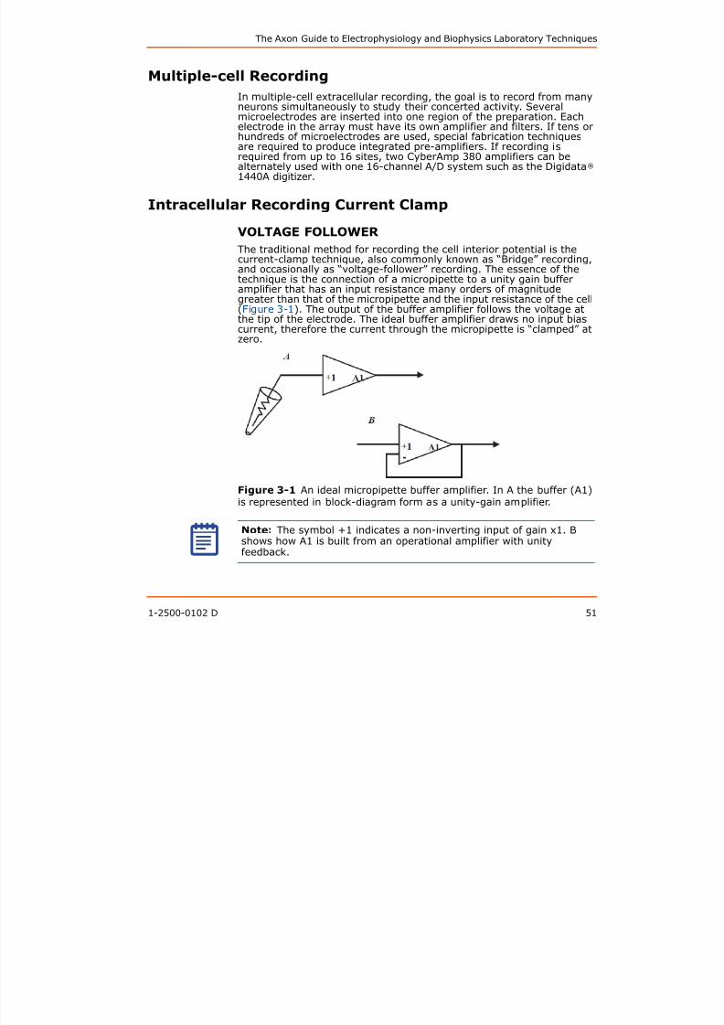
VOLTAGE FOLLOWER
The traditional method for recording the cell interior potential is thecurrent-clamp technique, also commonly known as “Bridge” recording,and occasionally as “voltage-follower” recording. The essence of thetechnique is the connection of a micropipette to a unity gain bufferamplifier that has an input resistance many orders of magnitudegreater than that of the micropipette and the input resistance of the cell(Figure 3-1). The output of the buffer amplifier follows the voltage atthe tip of the electrode. The ideal buffer amplifier draws no input biascurrent, therefore the current through the micropipette is “clamped” atzero.
Figure 3-1 An ideal micropipette buffer amplifier. In A the buffer (A1)is represented in block-diagram form as a unity-gain amplifier.
Note: The symbol +1 indicates a non-inverting input of gain x1. Bshows how A1 is built from an operational amplifier with unityfeedback.
Instrumentation for Measuring Bioelectric Signals from Cells
If a high-quality current injection circuit (current source) is connectedto the input node all of the injected current flows down the

8/13/2019 User Guide v3
http://slidepdf.com/reader/full/user-guide-v3 53/302
52 1-2500-0102 D
to the input node, all of the injected current flows down themicropipette and into the cell (see Figure 3-2). The current source can
be used to inject a pulse of current to stimulate the cell, a DC current todepolarize or hyperpolarize the cell, or any variable waveform that theuser introduces into the control input of the current source.
Figure 3-2 A high-quality current source.
A high-quality current source can be made by adding a second amplifierto the buffer amplifier circuit. The inputs to A2 are a command voltage,
Vcmd, and the pipette voltage (Vp) buffered by A1. The voltage acrossthe output resistor, Ro, is equal to Vcmd regardless of Vp. Thus thecurrent through Ro is given exactly by I = Vcmd /Ro. If stray capacitancesare ignored, all of this current flows through the pipette into the cell,then out through the cell membrane into the bath grounding electrode.
Bridge Balance
Can the intracellular potential be measured if the current injected downthe micropipette is a variable waveform? Without special compensationcircuitry, the answer is no. The variable current waveform causes acorresponding voltage drop across the micropipette. It is too difficult todistinguish the intracellular potential from the changing voltage dropacross the micropipette. However, special compensation circuitry canbe used to eliminate the micropipette voltage drop from the recording.The essence of the technique is to generate a signal that is proportionalto the product of the micropipette current and the micropipetteresistance. This signal is then subtracted from the buffer amplifieroutput (Figure 3-3). This subtraction technique is commonly known as
The Axon Guide to Electrophysiology and Biophysics Laboratory Techniques
“Bridge Balance” because in the early days of micropipette recording, aresistive circuit known as a “Wheatstone Bridge” was used to achieve

8/13/2019 User Guide v3
http://slidepdf.com/reader/full/user-guide-v3 54/302
1-2500-0102 D 53
resistive circuit known as a Wheatstone Bridge was used to achievethe subtraction. In all modern micropipette amplifiers, operational
amplifier circuits are used to generate the subtraction, but the namehas persisted.
Figure 3-3 The “Bridge Balance” technique.
This technique is used to separate the membrane potential (Vm) fromthe total potential (Vp) recorded by the micropipette. The technique isschematically represented in A. A differential amplifier is used tosubtract a scaled fraction of the current (I) from Vp. The scaling factoris the micropipette resistance (Rp). The traces in B illustrate theoperation of the bridge circuit. When the current is stepped to a newvalue, there is a rapid voltage step on Vp due to the ohmic voltage dropacross the micropipette. Since the micropipette is intracellular, changesin Vm are included in Vp. Thus the Vp trace shows an exponential rise toa new potential followed by some membrane potential activity. Thebridge amplifier removes the instantaneous voltage step, leaving theVm trace shown.
There are several ways to set the bridge balance. A commonly usedtechnique is to apply brief repetitive pulses of current to themicropipette while it is immersed in the preparation bath. The BridgeBalance control is advanced until the steady-state pulse response is
Instrumentation for Measuring Bioelectric Signals from Cells
eliminated (Figure 3-4). At this point, the circuit is balanced and themicropipette resistance can be read from the calibrated readout of the

8/13/2019 User Guide v3
http://slidepdf.com/reader/full/user-guide-v3 55/302
54 1-2500-0102 D
micropipette resistance can be read from the calibrated readout of theBridge Balance control. The same technique can even be used after the
micropipette has penetrated the cell. Details of how to achieve this aredescribed in the Axoclamp 900A and MultiClamp 700B manuals.
Figure 3-4 Illustration of bridge balancing while micropipette isextracellular.
All traces show the Vm output from the bridge-balance circuit. A 5 nA,2 ms pulse is applied to a 50 MΩ electrode. No bridge balance is usedin the left trace, revealing the full voltage drop across the micropipette.In the middle trace, optimum bridge balance is used and the voltagedrop across the micropipette is eliminated from the record. Thetransients at the onset and finish of the step result from the finitebandwidth of the headstage amplifier. In the right trace, thebridge-balance control is advanced too far; the voltage drop across themicropipette is overcompensated and a reverse-polarity step appears.
It is important that the micropipette resistance be constant. Clearly, ifthe micropipette resistance varies as the current flows there will be nounique setting of the Bridge Balance control and the measurement willinclude an artifact due to the variable voltage drop across themicropipette.
Junction PotentialsA second extraneous contributor to the measured voltage at the outputof the micropipette buffer amplifier is the sum of the junctionpotentials. Junction potentials occur wherever dissimilar conductors arein contact. The largest junction potentials occur at the liquid-metal junction formed where the wire from the amplifier input contacts theelectrolyte in the micropipette and at the liquid-liquid junction formedat the tip of the micropipette. The sum of all of the junction potentialscan be eliminated by introducing a single DC potential of the opposite
The Axon Guide to Electrophysiology and Biophysics Laboratory Techniques
polarity. In micropipette experiments, the junction potentials can oftensum to a few hundred millivolts. The ±500 mV range of the offset
8/13/2019 User Guide v3
http://slidepdf.com/reader/full/user-guide-v3 56/302
1-2500-0102 D 55
gcontrols provided by all Axon Conventional Electrophysiology
microelectrode amplifiers is more than sufficient to compensate foreven the worst-case junction potentials.
Track
A special form of automatic offset compensation is available in manypatch clamp amplifiers, including the Axopatch™-1 and the Axopatch200 amplifier series. In Axopatch amplifiers this technique is called “Track.” In some instruments of other manufacturers it is called “Search.” The Track circuit is used only during seal formation. During
seal formation the tip comes in and out of contact with the membraneand rapid shifts in the tip potential of the headstage sometimes occur.These potential shifts lead to equivalent rapid shifts in the currentrecord, which may exceed the dynamic range of the headstage. Sincethe headstage itself saturates, AC coupling at the oscilloscope or anyother form of external DC offset removal will not be useful. Instead, theTrack circuit dynamically adjusts the offset potential of the micropipetteitself, so that the current is forced to be zero on average. It is importantthat the Track circuit be switched off before recording of ionic currents
commences since the Track circuit introduces the same type ofdistortion produced by AC coupling.
Current Monitor
Current-clamp circuits include a monitor output proportional to thecurrent waveform. In some current-clamp amplifiers, the monitoroutput is merely a scaled version of the control voltage driving thecurrent-clamp circuit. As long as the micropipette resistance ismoderate and the current-clamp circuit output does not exceed its
linear operating range, this technique is accurate. However, if themicropipette resistance is very high and the current-clamp circuitrysaturates, the actual current through the micropipette will be less thanthe expected current. This simple monitor output will not indicate thefailure to pass the expected current. A better technique is to actuallymeasure the current by monitoring the voltage drop across a resistor inseries with the micropipette (Figure 3-5). This is a superior techniqueused in all of Axon’s micropipette current-clamp amplifiers, includingthe Axoclamp 900A and MultiClamp 700A and 700B.
Instrumentation for Measuring Bioelectric Signals from Cells

8/13/2019 User Guide v3
http://slidepdf.com/reader/full/user-guide-v3 57/302
56 1-2500-0102 D
Figure 3-5 Series current measurement.
The circuit in Figure 3-2 is extended by the addition of a differentialamplifier (A3) to measure the voltage drop across the current settingresistor, Ro. This voltage drop is proportional to the total current (I)flowing through Ro. For high-frequency currents (for example, thetransient current during a step change in the command potential), thecurrent through Ro is not quite identical to the membrane current (Im).There is an additional current that flows through the capacitance (Cw)of the wall of the micropipette and another current that flows into theinput capacitance (Cin) of the amplifier. Nevertheless, if precautions aretaken to minimize Cw (for example, shallow bath immersion, Sylgard ormineral oil coating) and Cin (for example, bootstrapped buffer amplifier,capacitance neutralization), the error current in these straycapacitances can be minimized and the output signal, VI, is a goodrepresentation of the membrane current.
Another way to measure the true micropipette current is to use aseparate circuit called a “virtual ground” (Figure 3-6). Instead ofconnecting the bath ground electrode directly to ground, it is connectedto the virtual ground formed at the negative input of an invertingoperational amplifier. The negative input in this configuration is called a “virtual” ground because the operational amplifier endeavors to keepthe negative input equal to the ground potential at the positive input.To achieve this goal, the operational amplifier output must continuouslypass a current through the feedback resistor (into the node at thenegative input) that is equal and opposite to the bath ground current.
The Axon Guide to Electrophysiology and Biophysics Laboratory Techniques
Thus the voltage at the output of the operational amplifier is directlyproportional to the bath current.

8/13/2019 User Guide v3
http://slidepdf.com/reader/full/user-guide-v3 58/302
1-2500-0102 D 57
Figure 3-6 Virtual-ground current measurement.
The bath grounding electrode is connected to the negative input ofoperational amplifier A3. The output (VI) continually adjusts to passcurrent through the feedback resistor (Rf ) equal and opposite to thetotal current flowing into the junction at the negative input of A3. Thepotential at the negative input is “virtually” equal to ground at all times.Most of the current measured by A3 is the membrane current, Im.However, during rapid potential changes, transient current flowsthrough the capacitance (Cw) of the wall of the micropipette and the
input capacitance (Cin) of the amplifier. The current (Iw) through Cw flows into the bath and is recorded by the virtual-ground circuit. The current(Iin) through Cin flows into the system ground and is not recorded by thevirtual-ground circuit.
Since the series current-measurement technique is much moreconvenient, it is routinely used in preference to the virtual-groundcurrent-measurement technique. The virtual-ground technique isinconvenient for several reasons:
Instrumentation for Measuring Bioelectric Signals from Cells
1. The input lead to the virtual ground is very sensitive and easilypicks up line-frequency and other interference.

8/13/2019 User Guide v3
http://slidepdf.com/reader/full/user-guide-v3 59/302
58 1-2500-0102 D
2. It is extremely difficult to use two microelectrode amplifiers inthe same preparation bath if one or both of them uses avirtual-ground current-measurement circuit. If one amplifieruses a virtual ground, the individual micropipette currents willbe difficult to identify because the virtual-ground currentmonitor measures the summed current from all sources. If twoamplifiers use a virtual ground, large DC-error currents will flowbetween the virtual-ground circuits because of the smalldifferences in offset voltages between the two circuits. This isequivalent to the problem that would exist if two voltage sources
were connected in parallel.3. The virtual-ground probe is just one more box of electronics that
has to be mounted in the crowded space around the preparationbath.
Nevertheless, the virtual ground technique is still used in somecircumstances, most commonly with high-voltage two-electrodevoltage-clamp amplifiers, because of the technical difficulty of making aseries current-measurement circuit operate at high voltages.
The Bath Error Potentials section below describes an importantvariation on the virtual-ground design to eliminate the voltage errordue to current flow through the grounding electrode.
Headstage Current Gain
The HS-9A and HS-2A headstages used with the Axoclamp 900A andAxoclamp 2B amplifiers all have unity voltage gain but come in avariety of current-passing capabilities. The current-passing range andresolution are determined by the size of a single resistor in the
headstage. This resistor (Ro) has two functions. In addition todetermining the size and resolution of the current that can be passed, italso determines the sensitivity with which current is measured. In thestandard HS-9A headstage, Ro is 10 MΩ; this is arbitrarily assigned acurrent-passing gain of H = 1. To pass more current, a headstage witha smaller value of Ro is required. The headstage with Ro = 1 MΩ canpass ten times as much current as the standard headstage; it isassigned a current-passing gain of H = 10. The headstage designed forion-sensitive micropipettes can only pass very tiny currents. The value
of Ro in this headstage is 100 GΩ; the current-passing gain isH = 0.0001.
Capacitance Compensation
The high-frequency performance of the micropipette amplifier iscompromised by the presence of capacitance at the amplifier input.This capacitance comes from several sources: the capacitance acrossthe glass wall (transmural capacitance) of the immersed part of the
The Axon Guide to Electrophysiology and Biophysics Laboratory Techniques
micropipette; the stray capacitance from the rest of the micropipette tonearby grounded surfaces; the stray capacitance from the micropipetteholder; and the capacitance to ground at the input of the buffer
8/13/2019 User Guide v3
http://slidepdf.com/reader/full/user-guide-v3 60/302
1-2500-0102 D 59
holder; and the capacitance to ground at the input of the buffer
operational amplifier.The input capacitance and the micropipette form a simple low-passfilter. That is, high-frequency signals at the tip of the micropipette areshunted to ground by the input capacitance. There are several ways toimprove the bandwidth of the recording system.
The best is to minimize the physical magnitude of the various elementscontributing to the input capacitance. The transmural capacitance ofthe immersed part of the micropipette can be quite large. Typically, it is1 pF or more per millimeter of immersion depth. An effective way to
reduce this capacitance is to thicken the wall of the micropipette. Thiscan be done by coating the micropipette with Sylgard or an equivalentmaterial (see Chapter 4: Microelectrodes and Micropipettes onpage 117). Other materials have been used, and in extreme cases,researchers have used a wide micropipette to form a jacket over thenarrower recording micropipette.
The other obvious way to reduce the transmural capacitance is toreduce the fluid level so that the immersion depth is minimal. This isnot always as effective as might be expected, because surface tension
causes the bath solution to creep up the surface of the micropipette.This generates significant capacitance between the inside of themicropipette and the film of solution on the outside. Forming this filmcan be prevented by making the surface of the micropipettehydrophobic by dipping the filled micropipette into mineral oil (orsilane) immediately before using it. Note that it is essential to fill themicropipette first with the aqueous electrolyte pipette solution so thatthe aqueous solution prevents the mineral oil from entering the tip.Finally, one should try not to place the holder or the microelectrode tooclose to grounded surfaces (such as the microscope objective).
Once the physical magnitude of the stray capacitance has beenminimized, electrical techniques can be used to reduce the effectivemagnitude. There are three such techniques:
1. Some researchers surround the micropipette with a metal shieldthat is connected to the unity-gain output of the buffer amplifier.The principle here is to make sure that the stray capacitancedoes not have a signal voltage across it. As long as there is nosignal voltage across the capacitance, no high-frequency current
is drawn and the bandwidth is increased. Unfortunately, thistechnique can significantly compromise the noise performanceof the amplifier because random noise generated in the bufferamplifier is coupled back into its input via the shieldcapacitance. For this reason, Molecular Devices does notrecommend the use of a driven shield.
2. Unity-gain feedback can be used to reduce the component ofstray capacitance that exists between the amplifier input and itspower supplies and case (Figure 3-7). In a technique known as
Instrumentation for Measuring Bioelectric Signals from Cells
“bootstrapping,” sophisticated circuitry is used to superimposethe unity-gain output of the buffer amplifier back onto its ownpower supplies and the headstage case. This eliminates the

8/13/2019 User Guide v3
http://slidepdf.com/reader/full/user-guide-v3 61/302
60 1-2500-0102 D
power supplies and the headstage case. This eliminates the
high-frequency current loss through the power supplycapacitance and consequently increases the bandwidth. Sincethe power supply capacitance is present whether or not thepower supply is bootstrapped, there is no noise penalty due toimplementing the technique. Bootstrapped power supplies areimplemented in the Axoclamp 900A and MultiClamp 700Bamplifiers and contribute to their excellent noise and bandwidthcharacteristics.
Figure 3-7 Bootstrapped power supplies.
Bootstrapped power supplies are used to increase the bandwidthby minimizing the high-frequency current loss through thepower-supply capacitance. The power-supply capacitance ismade up of C+ and C- from the positive input of A1 to thepositive and negative power supplies, respectively. All of thestray capacitances other than C+ and C- are lumped togetherand called Cext in this figure. The power supplies of A1 arebatteries. The center point of the batteries is connected to abuffered version of Vp. If the batteries are 10 V, the powersupplies for A1 are (Vp + 10 V) and (Vp – 10 V). The voltages
across C+ and C- are constant at +10 V and -10 V, respectively.Hence, there are no transient currents in neither C+ nor C-,except at very high frequencies where these simple amplifiermodels are not appropriate. To ensure stability, the bandwidth ofA2 must be half or less of the bandwidth of A1. In practicalimplementations such as the MultiClamp 700B and Axoclamp900A microelectrode amplifiers, the batteries are simulated byelectronics.
The Axon Guide to Electrophysiology and Biophysics Laboratory Techniques
3. Finally, but not least, the technique known as “capacitancecompensation” or “negative capacitance” can be used to reducethe effective value of whatever capacitance remains. An

8/13/2019 User Guide v3
http://slidepdf.com/reader/full/user-guide-v3 62/302
1-2500-0102 D 61
p
amplifier at the output of the unity-gain buffer drives a current-injection capacitor connected to the input (Figure 3-8). At theideal setting of the amplifier gain, the current injected by theinjection capacitor is exactly equal to the current that passesthrough the stray capacitance to ground. If the amplifier gain isincreased past the ideal setting, the current injected back intothe input will cause the input signal to overshoot. As the gain isincreased past a certain setting, the circuit will oscillate withpotentially disastrous consequences for the cell.
Figure 3-8 Capacitance neutralization circuit.
Amplifier A2 places a voltage proportional to the pipette potential (Vp)across the capacitance-neutralization capacitor (Cn). At a particularsetting of the gain (kn) of A2, the current (In) through Cn is exactlyequal to the current (Iin) through the stray capacitance (Cin) at theinput of A1. By conservation of current, the pipette current (Ip) is zero.In the ideal case, the effective capacitance loading the pipetteresistance (Rp) is zero and the bandwidth is therefore very high. Inpractice, limitations due to the finite bandwidth of the amplifiers, thedistributed nature of Cin and other second-order effects limit therecording bandwidth.
An important consideration in the design of a capacitance neutralizationcircuit is to avoid introducing much additional noise from the circuitryitself. Low-noise amplifiers must be used and the size of the injectioncapacitor must be small. Axon Cellular Neuroscience HS-2 seriesheadstages were produced in two varieties. The low-noise “L” seriesheadstages used a 3 pF injection capacitor. The medium-noise “M”series headstages used a 10 pF injection capacitor. Generally, the Mseries headstages were only used for the current-passing micropipette
Instrumentation for Measuring Bioelectric Signals from Cells
(ME2 on an Axoclamp 900A amplifier) in a two-micropipettevoltage-clamp setup. Noise in this micropipette is less important thannoise in the voltage recording micropipette (ME1), and it is sometimes
8/13/2019 User Guide v3
http://slidepdf.com/reader/full/user-guide-v3 63/302
62 1-2500-0102 D
g g p p ( )
useful to have a larger compensation range on the current-passingmicropipette.
With the Axoclamp 900A amplifier, the HS-9A headstage series wasintroduced. These headstages have an increased capacitanceneutralization range (-10 to 35.5 pF), independent of the gain of theheadstage. These headstages can be used equally effectively asvoltage-recording or current-passing electrodes with the Axoclamp900A amplifier. The choice of HS-9A headstages for TEVC depends onthe size of the typical current to be measured.
A problem often encountered in TEVC is saturation of the amplifieroutput, because of the limits imposed by the power supply ultimatelysupplying the current to the microelectrode. If the optimum gain of thecapacitance neutralization amplifier is moderately high, (for example,2), the amplifier may saturate during large signals. In manyexperiments, large inputs would be unusual, and even if they occurredthe speed penalty incurred would not be disastrous. However, intwo-electrode voltage clamp experiments, large signal excursions arecommon and speed is crucial. To eliminate the saturation of thecapacitance compensation circuit, the Axoclamp 900A amplifier uses±180 V amplifiers in the capacitance neutralization circuit intwo-electrode voltage clamp mode.
If everything were ideal, the bandwidth of the recording system wouldapproach the bandwidth of the buffer amplifier alone (typically a fewmegahertz). However, in practice the bandwidth is limited by the phasedelays in the capacitance compensation pathway, and by the falseassumption that the stray capacitance can be represented by a lumpedcapacitor at the input of the amplifier. The capacitance is distributedalong the length of the micropipette. Nevertheless, the techniquesdescribed above can be used to substantially improve the bandwidth. Itis not unusual to achieve bandwidths of 30 kHz with micropipettes thatwould have a bandwidth of just one or two kilohertz if the abovetechniques were not implemented.
Leakage Current
Ideally, a micropipette headstage should pass zero current into themicropipette when the current command is at zero. In practice, there is
a leakage current created from two sources. The first is the inherentbias current of the operational amplifier’s input. This is usually of theorder of a few picoamps or less. The second is the current that flowsthrough the current injection resistor (Ro in Figure 3-2) because ofvoltage offsets in the current-control circuitry. A trim potentiometer canbe used to reduce this offset. In fact, an optimal setting can be foundwhere a small offset is left across Ro so that the resistor currentcompensates the operational amplifier bias current and leaves a netzero current through the micropipette. However, the leakage current
The Axon Guide to Electrophysiology and Biophysics Laboratory Techniques
will quickly grow again to unacceptable levels if the offsets in thecontrol circuitry change significantly with temperature or time. To avoidthis problem, Molecular Devices uses extremely high-quality, low-drift

8/13/2019 User Guide v3
http://slidepdf.com/reader/full/user-guide-v3 64/302
1-2500-0102 D 63
operational amplifiers in its Axon Conventional Electrophysiologymicropipette amplifiers.
Headstages for Ion-sensitive Microelectrodes
The most demanding application in terms of low-leakage currentrequirements is the measurement of ion concentration using ion-sensitive microelectrodes (ISMs). In spite of the current popularityabout ion-sensitive intracellular dyes, ISMs are still the best meansavailable for determining extracellular and, in some cases, intracellular
ion concentrations. These electrodes can be very difficult to fabricatebecause of the efforts required to place the highly hydrophobicion-sensitive resin at the very tip of the electrode. Due to thehydrophobic nature of the liquid resin, ISMs are also very sensitive tocurrent passing into the electrode. Even the tiniest amount of leakagecurrent from the headstage can cause the resin to move. If the resinleaks out of the electrode it can contaminate the preparation anddestroy cells in the vicinity of the electrode. If the resin moves up thebarrel of the pipette, the response of the electrode is slowed
dramatically or destroyed.There are two ways to ensure low-leakage currents for thesemicroelectrodes: First, use special operational amplifiers that have biascurrents of just a few tens of femtoamps. Second, make the value of Ro very large (100 GΩ) so that the current induced by small offsetvoltages across Ro is small.
Bath Error Potentials
In most experiments, the bathing solution is grounded by a solidgrounding electrode (such as an Ag/AgCl pellet in the bath, or whichcan be connected to the bath via an agar/KCL bridge) and allmeasurements are made relative to ground, on the assumption that thebath is also at ground. This assumption may not be true in experimentsin which the Cl- concentration or temperature of the bathing solution issignificantly changed, or where the membrane current is sufficientlylarge to cause a significant voltage drop across the resistance of thegrounding electrode. The latter circumstance would normally occur onlywhen voltage clamping very large cells such as frog oocytes, in which
case the ionic current may be of the order of several microamps oreven several tens of microamps.
Depending upon the grounding method, the resistance of the bathgrounding electrode (Rb) could be as much as 10 kΩ, although withcare it is not difficult to achieve Rb values less than 1 kΩ.
In a simple two-electrode voltage clamp (TEVC) setup, the voltage dropacross Rb is indistinguishable from the membrane potential. That is, thepotential (V1) recorded by the voltage-recording micropipette is the
Instrumentation for Measuring Bioelectric Signals from Cells
sum of the transmembrane potential (Vm) and the bath potential (Vb).Problems arise if the product of the clamp current (I2) and Rb issignificant. For example, for I2 = 5 μA and Rb = 2 kΩ, the error voltage

8/13/2019 User Guide v3
http://slidepdf.com/reader/full/user-guide-v3 65/302
64 1-2500-0102 D
is 10 mV. In some experiments, a worst-case error of this magnitudemight be tolerable; but if the error were to be much greater, theposition of the peak of I-V curves and other responses would beseriously affected.
To faithfully record Vm, either Vb must be made equal to or nearly equalto zero, or the value of Vb must be independently measured andsubtracted from the potential recorded by ME1. There are severalmethods to choose from:
1. The best method is to minimize Rb in the first place.
2. Electronically predict and subtract the error voltage. Thistechnique is known as “series-resistance compensation.”
3. Use an independent electrode to measure Vb and subtract thisvalue from V1.
4. Set up an independent clamping circuit to clamp Vb, measurednear the surface of the cell, to zero.
5. Set up an independent virtual-ground circuit to clamp Vb,measured near the surface of the cell, to zero, while
simultaneously measuring the bath current.
Minimizing R b
There are three main contributors to Rb:
1. The cell access resistance from the membrane surface to thebath.
2. The resistance of an agar bridge, if used.
3. The resistance of the grounding wire.
Cell Access Resistance
The access resistance to a sphere is given by:
where ρ is the resistivity (typically 80 Ωcm for Ringer’s solutionat 20 °C [Hille, 1984]) and r is the radius of the sphere incentimeters.
Modeling an oocyte as a 1 mm diameter sphere:
Resistance of an Agar Bridge
The Axon Guide to Electrophysiology and Biophysics Laboratory Techniques
The resistance of a cylindrical agar bridge is given by (Hille,1984):
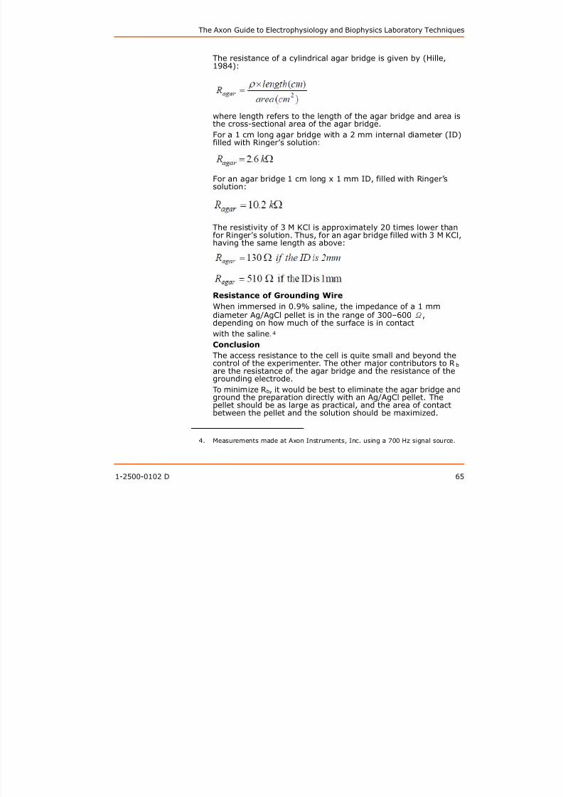
8/13/2019 User Guide v3
http://slidepdf.com/reader/full/user-guide-v3 66/302
1-2500-0102 D 65
where length refers to the length of the agar bridge and area isthe cross-sectional area of the agar bridge.
For a 1 cm long agar bridge with a 2 mm internal diameter (ID)filled with Ringer’s solution:
For an agar bridge 1 cm long x 1 mm ID, filled with Ringer’ssolution:
The resistivity of 3 M KCl is approximately 20 times lower thanfor Ringer’s solution. Thus, for an agar bridge filled with 3 M KCl,having the same length as above:
Resistance of Grounding Wire
When immersed in 0.9% saline, the impedance of a 1 mmdiameter Ag/AgCl pellet is in the range of 300–600 Ω,depending on how much of the surface is in contact
with the saline.4
Conclusion
The access resistance to the cell is quite small and beyond thecontrol of the experimenter. The other major contributors to Rb
are the resistance of the agar bridge and the resistance of the
grounding electrode.To minimize Rb, it would be best to eliminate the agar bridge andground the preparation directly with an Ag/AgCl pellet. Thepellet should be as large as practical, and the area of contactbetween the pellet and the solution should be maximized.
4. Measurements made at Axon Instruments, Inc. using a 700 Hz signal source.
Instrumentation for Measuring Bioelectric Signals from Cells
However, if the bathing solution is changed during theexperiment, the DC offset of the Ag/AgCl pellet will change withthe chloride activity. Thus, in this case it is essential to either

8/13/2019 User Guide v3
http://slidepdf.com/reader/full/user-guide-v3 67/302
66 1-2500-0102 D
use an agar bridge to prevent the DC offset of the bath fromchanging, or to use a bath-potential recording headstage with a3 M KCl electrode to follow and remove the shift. Anotheradvantage of an agar bridge is that it prevents metal ions fromthe grounding electrode from entering the bathing solution.
If an agar bridge is used, it is best to fill it with 3 M KCl insteadof Ringer’s solution in order to minimize Rb. When the agarbridge is filled with 3 M KCl, the sum of all components of Rb willbe approximately 1–2 kΩ. If leakage of KCl from the agar bridge
is a problem, it may be necessary to fill the agar bridge withRinger’s solution. In this case, Rb will be several kilohms ormore.
Series-Resistance Compensation
This sophisticated technique is used to minimize the effects of theelectrode resistance in a whole-cell voltage clamp. It is described laterin this chapter and is of paramount importance when there is noalternative available. However, series-resistance compensation is never
completely effective. The other methods discussed in this section aremore reliable and easier to apply when it comes to eliminating thevoltage error across Rb.
Measure and Subtract Vb
Another technique used to eliminate the effects of the IR voltage dropacross the bath resistance is to actively measure the bath potentialoutside the cell.
In this method, the bath is grounded by any preferred method. The
bath potential is allowed to shift because of solution changes,temperature changes or current flow. The changing values of the bathpotential (Vb) are continuously monitored by a 3 M KCl-filled electrodeplaced near the cell. The measured value of Vb is subtracted from thepotentials measured by the intracellular microelectrodes. Formicroelectrodes being used
for voltage recording, this subtraction yields the true transmembranepotential (Vm). The signal provided to all subsequent circuits in theamplifier is Vm.
This method operates well. The minor inconveniences are the morecomplex electronics, the noise of the bath electrode that is added to thenoise of the intracellular recording micropipette, and some (minor)potential for instability in a two-electrode voltage clamp if thebandwidth of the bath potential headstage is greater than thebandwidth of the intracellular recording micropipette.
The Axon Guide to Electrophysiology and Biophysics Laboratory Techniques
Clamp Vb Using a Bath Clamp
Another means to eliminate the effect of the voltage drop across Rb isto actively control the bath potential measured near the outside surface

8/13/2019 User Guide v3
http://slidepdf.com/reader/full/user-guide-v3 68/302
1-2500-0102 D 67
of the cell. This is achieved using a two-electrode virtual-ground circuit(Figure 3-9). One electrode (SENSE) is a voltagesensing electrode. Thiselectrode is placed in the preparation bath near the cell surface. It isconnected to the virtual-ground circuit by an agar bridge or othermeans, of resistance Rb2. Since there is no current flow through thiselectrode, there is no voltage drop across Rb2. The other electrode(IBATH) is placed in the preparation bath. This electrode carries the ioniccurrent. The feedback action of the operational amplifier ensures thatthe potential at the SENSE electrode is equal to the potential at the
negative amplifier input (ignoring the offset voltage at the inputs to theoperational amplifier).
Figure 3-9 Two-electrode virtual-ground circuit.
In this implementation, separate electrodes are used to pass the bathcurrent and control the bath potential (unlike Figure 3-6 above). Thebasic operation is the same as for the virtual-ground circuit describedearlier, except that instead of connecting the feedback resistor directlyto the negative input of the operational amplifier, it is connectedindirectly via the bath solution. The bath potential near the surface ofthe cell is recorded by the SENSE electrode (resistance Rb2) and forcedby the feedback action of the operational amplifier to be near ground.The bath current required to achieve this is passed by the operationalamplifier through the feedback resistor (Rf ) and through the bath
current electrode (IBATH; resistance Rb1).
Clamp Vb Using a Virtual-Ground Current Monitor
This technique is identical to the bath clamp described above, exceptthat in this case instead of being ignored, the output of the circuit isused to monitor the current flowing from the micropipettes into thebath. The output (VI) of this circuit is proportional to the bath current.
Instrumentation for Measuring Bioelectric Signals from Cells
There are several problems with this technique. First, if the output is

8/13/2019 User Guide v3
http://slidepdf.com/reader/full/user-guide-v3 69/302
68 1-2500-0102 D
used to record the bath current, it is usual to ignore the Rb1 term(because its value is unknown) and to assume that
Thus, there is a small error equal to Rb1 /(Rb1 + Rf ). Second, if there arefluid-filled tubes connected to the bath, and if some of these runoutside of the Faraday cage, they will act as antennas and conduct a lotof hum current into the bath that will be recorded by the virtual-groundcircuit. Third, if it is desired to use more than one amplifier with the
same preparation, it is essential that no more than one of them uses avirtual-ground circuit to clamp the bath potential. This is not a seriousproblem, since it is easy to make one virtual-ground serve the needs ofboth amplifiers. The problem is serious, however, if one of theamplifiers introduces command signals via the virtual-ground bathclamp. This is a practice employed by some manufacturers because insome circumstances it is easier to design the electronics for this modeof operation. However, if command potentials are introduced via thebath electrode, it is extremely difficult to perform experiments usingtwo amplifiers, for example, whole-cell patch clamp of two fused cells.
When used with consideration for the measurement error, and if humpick up is avoided, a virtual-ground circuit to measure IBATH offersexcellent performance.
Summary
As a first priority, we recommend that the value of Rb be minimized bythe techniques described above. If it is still considered to be importantto compensate for the IR voltage drop, a virtual-ground headstage
(such as the VG-9A series) can be used to clamp the bath potential, ora unity-gain voltage follower headstage (such as the HS-9A andHS-2A series) can be used to record and subtract the bath potential.
Cell Penetration: Mechanical Vibration,Buzz, and Clear
Often when a micropipette is pressed against a cell, the membranedimples but the micropipette fails to penetrate. A variety of methods
are used to overcome this problem. The oldest and frequently effectivetrick is to tap the micromanipulator gently. Since this “method” isdifficult to calibrate and reproduce, two electronic alternatives arewidely used. One is to drive a brief, high-frequency oscillatory currentthrough the micropipette. This is often done by briefly increasing thecapacitance compensation such that the compensation circuit oscillates.On the Axoclamp amplifiers, a dedicated feature called "Buzz" isprovided for this purpose. On the Axoclamp 900A amplifier, this featurehas a duration control setting; on the Axoclamp 2B amplifier, buzz
The Axon Guide to Electrophysiology and Biophysics Laboratory Techniques
duration can also be controlled via its remote buzz accessory unit. Theduration used should be long enough for penetration, but short enoughto prevent damage to the cell. The mechanism of penetration isunknown, but it may involve attraction between the charge at the tip ofth i i tt d b d h th i id f th b
8/13/2019 User Guide v3
http://slidepdf.com/reader/full/user-guide-v3 70/302
1-2500-0102 D 69
the micropipette and bound charges on the inside of the membrane.
The second electronic alternative is to drive a large positive or negativecurrent step into the cell.
In the Axoclamp 900A amplifier, both the duration and height of thecurrent pulse are adjustable. Again, the mechanism of penetration isnot known. One cannot even predict whether a positive or a negativepulse will be more effective.
None of the three methods described here can be described as “best.”
For a particular cell type, the researcher must experiment to find themethod that works best with those cells.
Command Generation
In general, current and voltage commands arise from a variety ofsources: internal oscillators in the instrument, internal DC current orvoltage controls, external input from a computer, etc. These commandsare usually summed in the instrument so that, for example, an
externally generated step command can be superimposed on theinternally generated holding potential.
An important consideration when using externally generated commandsis the attenuation provided by the instrument’s command input.Manufacturers attenuate the external command so that the effects ofnoise and offset in the external signal generator are minimized. Noise isparticularly common on the analog output of most computer interfaces.To illustrate the problem, imagine a micropipette amplifier used forcurrent injection into cells that has a current passing capacity of
±100 nA maximum. Compare the situation for two different values ofthe command input attenuation. In the first case, the amplifier passes1 nA for each millivolt from the computer. If there is a 2 mV of wide-band digital noise on the output of the D/A converter, this will generate2 nA of noise in the recording a substantial fraction of the usable range.Further, if the D/A converter had a 3 mV offset, then instead of acommand of zero generating 0 nA, it would generate 3 nA. In thesecond case, the amplifier passes 1 nA for each 100 mV from thecomputer. This time, the 2 nA of noise from the D/A converter onlygenerates 20 pA of noise in the recording, and the 3 mV offset error
only generates a 30 pA current error. The full ±100 nA range of theamplifier can still be controlled, since most D/A converters produce upto ±10 V.
All of the Axon Conventional Electrophysiology current-clamp andvoltage-clamp instruments from Molecular Devices use the maximumpossible attenuation so that the ±10.24 V output from the D/Aconverter corresponds to the normal maximum operating limits of theinstrument.
Instrumentation for Measuring Bioelectric Signals from Cells
Another important consideration when using externally generatedcommands is the presence or absence of polarity inversion. To minimizethe risk of making mistakes during an experiment, it is best that theinstrument does not invert the command signal. Thus the user shouldalways know that a positive command from the computer will generate

8/13/2019 User Guide v3
http://slidepdf.com/reader/full/user-guide-v3 71/302
70 1-2500-0102 D
always know that a positive command from the computer will generatea positive current or voltage in the instrument.
Intracellular Recording—Voltage Clamp
In the voltage-clamp technique, the membrane potential is heldconstant (for example, “clamped”) while the current flowing throughthe membrane is measured. Usually, the investigator has no inherent
interest in the membrane current, but is interested in the membraneconductance, since conductance is directly proportional to the ion-channel activity. Current is measured because the investigator has nodirect way of measuring conductance. By holding the membranepotential constant (or at the very least, constant after a rapid step), theinvestigator ensures that the current is linearly proportional to theconductance being studied.
Micropipette voltage-clamp techniques for whole-cell currentmeasurement traditionally assign the role of potential measurement
and current passing to two different intracellular micropipettes. This isdone using the conventional two-electrode voltage-clamp technique, orit is simulated by time-division multiplexing (time-sharing) using thediscontinuous single-electrode voltage-clamp technique. Separation ofthe micropipette roles by either of these methods avoids theintroduction of errors in the measurement due to unknown andunstable voltage drops across the series resistance of the current-passing micropipette.
The so-called “whole-cell patch” voltage clamp is a technique wherein
only one micropipette is used full-time for both voltage recording andcurrent passing. A method known as series-resistance compensation(see Series-Resistance Compensation on page 86) attempts toeliminate the aberrations arising when one micropipette is made toperform the work of two. For series-resistance compensation to work,the micropipette resistance must be reasonably low compared to theimpedance of the cell. Since the resistance of intracellular micropipettesgenerally is too high, researchers use very blunt micropipettes that canbe tightly sealed to a patch of membrane. The patch of membrane issubsequently ruptured so that the micropipette provides a
low-resistance access to the whole cell, hence the term “whole-cellpatch” clamp.
The Ideal Voltage Clamp
The ideal voltage clamp simply consists of a battery, a switch, a wire,the cell and an ammeter (Figure 3-10). Since the wire has zeroresistance when the switch is closed, the membrane potential steps
The Axon Guide to Electrophysiology and Biophysics Laboratory Techniques
instantly to the battery voltage. This generates an impulse of currentthat charges the membrane capacitance, followed by a steady-statecurrent to sustain the voltage across the membrane resistance.

8/13/2019 User Guide v3
http://slidepdf.com/reader/full/user-guide-v3 72/302
1-2500-0102 D 71
Figure 3-10 The ideal voltage clamp.
The ideal voltage clamp simply consists of a battery, a switch, a wire,the cell and an ammeter. When the switch closes, the membranepotential steps instantly to the battery voltage. (For simplicity, it isassumed that Vm = 0 before the step.) There is an impulse of currentinjecting a charge Q = CmVcmd; the steady-state current is Vcmd /Rm.
In this experiment, the voltage is the independent variable. Its value iscontrolled and equal to the battery value. The current is the dependentvariable; its value is measured by an ammeter. For this reason, thevoltage-clamp circuit is sometimes called a “current follower.”
Real Voltage Clamps
There are many reasons for real voltage clamps to be inferior to theideal voltage clamp. These include finite resistance of the current-passing micropipette, limited bandwidth of the voltage-recordingmicropipette, capacitive coupling between the two micropipettes,limited bandwidth of the clamp amplifier, and non-ideal phase shifts inthe membrane. These phenomena and the minimization of their impactare discussed in the following sections.
Large Cells—Two-Electrode Voltage Clamp
The theory of two-electrode voltage clamping is discussed in detail byFinkel and Gage (1985). Without attempting to duplicate thatdiscussion, some of the most important conclusions will be presentedhere.
Instrumentation for Measuring Bioelectric Signals from Cells
A conventional two-electrode voltage clamp is shown in Figure . Thisfigure has been simplified by ignoring several frequency-dependentcomponents: the input capacitance at the input of micropipette ME1,the coupling capacitance between the micropipettes, and the specialphase lead and lag circuitry that is often introduced deliberately into

8/13/2019 User Guide v3
http://slidepdf.com/reader/full/user-guide-v3 73/302
72 1-2500-0102 D
phase lead and lag circuitry that is often introduced deliberately intothe electronics. Furthermore, series resistance in the membrane andthe bathing solution has been ignored. In the figure, the solefrequency-dependent component is the membrane capacitance.
Figure 3-11 Conventional two-electrode voltage clamp.
A The membrane potential (Vm) is recorded by a unity-gain bufferamplifier (A1) connected to the voltage-recording microelectrode (ME1).Vm is compared to the command potential (Vcmd) in a high-gaindifferential amplifier (A2; gain = μ). The output of A2 is proportional tothe difference (ε) between Vm and Vcmd. The voltage at the output of A2forces current to flow through the current-passing microelectrode (ME2)into the cell. The polarity of the gain in A2 is such that the current inME2 reduces ε.
B Unlike the ideal case, there is a finite time required to charge the cellcapacitance. The time constant for the current and potential transientsis τ = Rp2Cm /μ, where Rp2 is the resistance of ME2. If was infinite, or ifRp2 was zero, the response would approach the ideal case.
The Axon Guide to Electrophysiology and Biophysics Laboratory Techniques
Error
The steady-state membrane potential (Vm) after a step change in thecommand voltage (Vcmd) is:

8/13/2019 User Guide v3
http://slidepdf.com/reader/full/user-guide-v3 74/302
1-2500-0102 D 73
where μ is the gain of the clamp amplifier and K is the attenuation ofthe clamp amplifier caused by the cell membrane resistance (Rm) andthe resistance (Rp2) of the output micropipette (ME2):
As the product μK becomes very large, the difference between Vm andVcmd becomes very small. Ideally, the error will be very low: just afraction of one percent. The gain of the clamp μ is typically set by afront-panel gain control in the range of about 100 to 10,000. If K wereunity, the error would vary from 1 percent down to 0.01 percent.However, if K is less than unity (as it always is), the error will be worse.If the output micropipette resistance is 90 MΩ and the membraneresistance is 10 MΩ, K is 0.1 and the error will be ten times worse thanif K were unity. If the two resistances are equal, K will be 0.5. Thus, asa rule of thumb it is desirable to use an output micropipette whoseresistance is as low as possible, ideally about the same size or smallerthan the membrane resistance.
Step Response and Bandwidth
After a step command, the membrane potential relaxes exponentially
towards its new value. For μK >> 1, the time constant for therelaxation is:
Increasing the clamp gain decreases the time constant for the stepresponse. For example, if Rp2 = 10 MΩ, Cm = 1000 pF and μ = 100, thetime constant is 100 μs.
Stated differently, increasing the clamp gain also increases thebandwidth with which Vm can follow changes in Vcmd. The -3 dBfrequency of the bandwidth is:
Instrumentation for Measuring Bioelectric Signals from Cells
Stability
The voltage clamp circuit shown in Figure 3-12 is unconditionallystable. The membrane capacitance provides a 90° phase shift, which is
required for stability in all negative feedback circuits. Unfortunately,th f t bi t k th i it t bl t hi h l i

8/13/2019 User Guide v3
http://slidepdf.com/reader/full/user-guide-v3 75/302
74 1-2500-0102 D
q y g y,other factors combine to make the circuit unstable at high clamp gains.
The coupling capacitance (Cx) between the micropipettes is extremelydestabilizing. Values as small as 0.01 pF can lead to oscillation if μ hasa magnitude of several hundred or more. There are several ways tominimize this coupling capacitance. The two best ways are by:
1. Introducing the two micropipettes into the preparation at a wideangle, preferably greater than 90°.
2. Placing a grounded metal shield between the two micropipettes.This shield should be large enough to block all line-of-sightpathways between the two micropipettes and their holders.
Another destabilizing factor is the non-ideal nature of the membrane.In Figure 3-11, the membrane is simply modeled as a parallel resistorand capacitor. In practice, a distributed model applies. The capacitanceelements are themselves non-ideal; they should be modeled by anideal capacitor with a series-resistance component. For realmembranes, the phase shift at high frequencies is less than 90°. In the
Axoclamp 900A amplifier, a phaseshift control is included to allow theuser to empirically introduce a phase lag to the circuit to build the totalhigh-frequency phase shift up to 90°.
The input capacitance of the voltage-recording micropipette (ME1) addsanother frequency-dependent variable into the system that also tendsto decrease the stability. The effect of this input capacitance is usuallyminimized by carefully adjusting the capacitance neutralization controlto maximize the bandwidth of ME1.
Small instabilities in the voltage clamp usually show up as an overshoot
in the current and voltage responses. Full instability shows up as acontinuous oscillation that can destroy the cell. In some voltageclamps, special circuits are used to detect oscillations and takeappropriate action to avoid damage to the cell. The Axoclamp 2 seriesand the GeneClamp® 500 amplifiers do not include an oscillation guardcircuit. The Axoclamp 900A amplifier includes an oscillation detectionfeature that automatically reduces the voltage clamp gain, protectingthe cells from harm.
Membrane Conductance Changes
It can be shown that the current response to a step change in themembrane conductance is identical to the membrane potentialresponse to a step change in the command voltage. This is fortunate,because it means that if the voltage clamp is set up optimally byobserving the response to a repetitive command step, it is alsooptimally set up for measuring conductance changes. In order for thisequivalence to be maintained, it is essential that the experimenter not
The Axon Guide to Electrophysiology and Biophysics Laboratory Techniques
use tricks such as filtering the command voltage to eliminate anovershoot in the response. This is a bad practice because it disguisesthe dynamic performance of the clamp circuit.
Noise
8/13/2019 User Guide v3
http://slidepdf.com/reader/full/user-guide-v3 76/302
1-2500-0102 D 75
There are several sources of noise in a two-electrode voltage-clampcircuit, but the most important is the thermal and excess noise of theinput micropipette, ME1. To the voltage-clamp circuit, this noiseappears as an extra command signal. It is imposed across themembrane and leads to a noise current. Because of the membranecapacitance, this noise current increases directly with frequency in thebandwidths of interest. The magnitude of the noise is worst in cells withlarge Cm values.
Since the current noise increases with frequency, a single-pole filter isinadequate. An active two-pole filter is required at minimum; while afour-pole filter is preferred. The Axoclamp 900A amplifier includes afour-pole filter with a corner frequency up to 30 kHz on each output.The user can choose between a Bessel and a Butterworth filter.
Micropipette Selection
Ideally, both micropipettes should have very small resistances. The
resistance of ME1 should be small to minimize the micropipette noise,and the resistance of ME2 should be small to maximize the product μK.However, low-resistance micropipettes are more blunt thanhigh-resistance micropipettes and do more damage to the cell. Ingeneral, it is more important to use a low resistance micropipette forME2. If its value is high, the amplifier’s power supply will saturate at alower current, causing a voltage-clamp error because the ME2headstage cannot inject enough current to hold the membrane voltage “clamped.” As a result, the recorded data will be of dubious merit. Arelatively high-resistance micropipette for ME1 has its problems—increased noise and reduced bandwidth—but at least it does notintroduce an error.
Input vs. Output Offset Removal
Certain offset-removal circuits act only on the output signal delivered tothe oscilloscope or data acquisition system. Examples of these are theAC input of the oscilloscope itself, the DC-offset removal in theCyberAmp 380 amplifier, and the output offset controls in the Axoclamp
900A. Adjusting these controls does not affect the membrane currentsinjected through the micropipette.
On the other hand, some offset-removal circuits act on the input signalseen by the voltage-clamp circuit. For example, the micropipette-offsetcontrols alter the potential that is clamped by the voltage-clamp circuit.Thus the actual membrane potential is affected when these controls arealtered and, consequently, the membrane current is affected. Care
Instrumentation for Measuring Bioelectric Signals from Cells
should be taken not to alter the setting of an input-offset control oncethe experiment has begun.
Small Cells—Discontinuous Single-ElectrodeVoltage Clamp

8/13/2019 User Guide v3
http://slidepdf.com/reader/full/user-guide-v3 77/302
76 1-2500-0102 D
gVoltage Clamp
In discontinuous single-electrode voltage clamp (dSEVC), the tasks ofvoltage recording and current passing are allocated to the samemicropipette. Time-sharing techniques are used to prevent interactionsbetween the two tasks. The principles of operation are discussed indetail by Finkel and Redman (1985).
A block diagram and a timing diagram illustrating the technique are
shown in Figure 3-12. A single micropipette (ME1) penetrates the celland the voltage recorded (Vp) is buffered by a unity-gain headstage(A1). To begin the discussion, assume that Vp is exactly equal to theinstantaneous membrane potential (Vm). A sample-and-hold circuit(SH1) samples Vm and holds the recorded value (Vms) for the rest of thecycle.
The Axon Guide to Electrophysiology and Biophysics Laboratory Techniques

8/13/2019 User Guide v3
http://slidepdf.com/reader/full/user-guide-v3 78/302
1-2500-0102 D 77
Figure 3-12 Block diagram and timing waveforms.
Vms is compared with a command voltage (Vcmd) in a differentialamplifier (A2). The output of this amplifier becomes the input of a
Instrumentation for Measuring Bioelectric Signals from Cells
controlled-current source (CCS) if the switch S1 is in thecurrent-passing position.
The CCS injects a current into the micropipette that is directly
proportional to the voltage at the input of the CCS irrespective of theresistance of the micropipette. The gain of this transconductance circuiti G
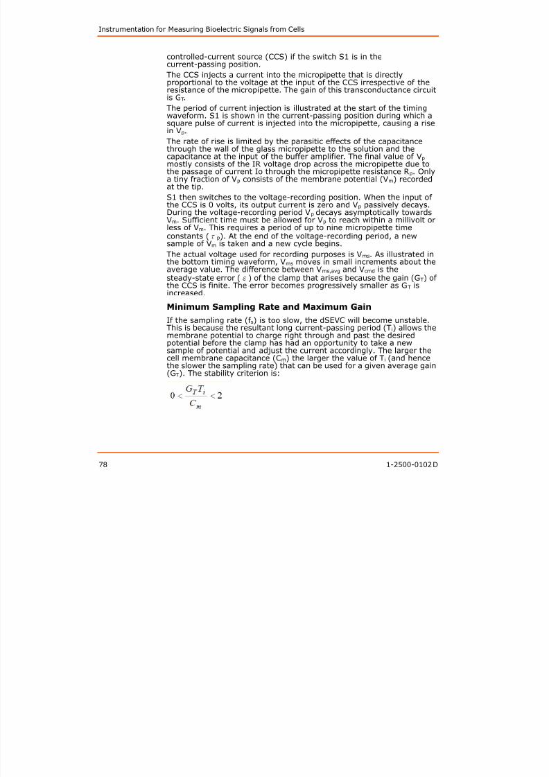
8/13/2019 User Guide v3
http://slidepdf.com/reader/full/user-guide-v3 79/302
78 1-2500-0102 D
is GT.
The period of current injection is illustrated at the start of the timingwaveform. S1 is shown in the current-passing position during which asquare pulse of current is injected into the micropipette, causing a risein Vp.
The rate of rise is limited by the parasitic effects of the capacitancethrough the wall of the glass micropipette to the solution and the
capacitance at the input of the buffer amplifier. The final value of Vp mostly consists of the IR voltage drop across the micropipette due tothe passage of current Io through the micropipette resistance Rp. Onlya tiny fraction of Vp consists of the membrane potential (Vm) recordedat the tip.
S1 then switches to the voltage-recording position. When the input ofthe CCS is 0 volts, its output current is zero and Vp passively decays.During the voltage-recording period Vp decays asymptotically towardsVm. Sufficient time must be allowed for Vp to reach within a millivolt or
less of Vm. This requires a period of up to nine micropipette timeconstants (τp). At the end of the voltage-recording period, a newsample of Vm is taken and a new cycle begins.
The actual voltage used for recording purposes is Vms. As illustrated inthe bottom timing waveform, Vms moves in small increments about theaverage value. The difference between Vms,avg and Vcmd is thesteady-state error (ε) of the clamp that arises because the gain (GT) ofthe CCS is finite. The error becomes progressively smaller as GT isincreased.
Minimum Sampling Rate and Maximum Gain
If the sampling rate (f s) is too slow, the dSEVC will become unstable.This is because the resultant long current-passing period (Ti) allows themembrane potential to charge right through and past the desiredpotential before the clamp has had an opportunity to take a newsample of potential and adjust the current accordingly. The larger thecell membrane capacitance (Cm) the larger the value of Ti (and hencethe slower the sampling rate) that can be used for a given average gain
(GT). The stability criterion is:
The Axon Guide to Electrophysiology and Biophysics Laboratory Techniques
For optimum response (critical damping) we require:
8/13/2019 User Guide v3
http://slidepdf.com/reader/full/user-guide-v3 80/302
1-2500-0102 D 79
Thus for a given GT, if Cm is small, Ti must be small (for example, f s mustbe large).
For example, if GT = 1 nA/mV and Cm = 100 pF, then Ti must be 100 μsfor optimum response. If Ti is greater than 100 μs, the step responsewill overshoot and at 200 μs the clamp will oscillate. (Note that inAxoclamp amplifiers, Ti = 100 μs corresponds to a sampling rate of3 kHz because the duty cycle (discussed later) is 30%.)
If Ti in this example cannot be as short as 100 μs because themicropipette response is too slow, then a lower value of GT will have tobe used to maintain optimum response.
Fastest Step Response
In a critically damped system, that is, where the gain has been turnedup to achieve the fastest possible response with no overshoot, theclamp can settle to its final value in as little as one or two periods.
Error Number One: Clamping the Micropipette
If the micropipette voltage does not have sufficient time to decay tozero before a new sample of Vm is taken, the sample will include amicropipette artifact voltage. The clamp circuit will be incapable ofdistinguishing this micropipette artifact voltage from the membranepotential and thus it will voltage clamp the sum of the two potentials.This leads to inaccurate and bizarre data collection. For example, cellswith known rectifiers will generate I-V curves that are almost linear.
This error is easily avoided by carefully observing the monitor output onthe Axoclamp 900A amplifier. It is essential that the micropipettevoltage trace on this output be given sufficient time to decay to zerobefore the sample is taken. The user can achieve this by adjusting thesampling frequency and by optimizing the micropipette capacitancecompensation. With the Axoclamp 900A amplifier, the micropipettevoltage monitor is transmitted to the computer through a USB 2.0connection. When dSEVC is activated, a window displaying themicropipette voltage is automatically displayed. This facilitates the
experimenter in observing the micropipette voltage and avoiding clamperrors.
Error Number Two: Steady-State Clamp Error
Even if the sampling is such that there is negligible voltage drop acrossthe micropipette, there will still be a steady-state error due to the finitegain, GT, of the clamp. To minimize the error, it is necessary to use ashigh a gain setting as possible, consistent with stable operation.
Instrumentation for Measuring Bioelectric Signals from Cells
Ripple in the Membrane Potential
Due to the switching nature of the dSEVC circuit, the actual membranepotential changes during each cycle. The size of the ripple is
proportional to the command voltage; for a clamp at the restingmembrane potential, the ripple is zero. Typically, the ripple is no moreth t t f th d lt Th t l

8/13/2019 User Guide v3
http://slidepdf.com/reader/full/user-guide-v3 81/302
80 1-2500-0102 D
than one or two percent of the command voltage. The actual errorbetween Vm and Vcmd is worst at the end of each cycle, just when thesample is taken. Therefore, the presence of ripple means that theaverage value of Vm is closer to Vcmd than is suggested by the sampledvoltages.
Aliased Noise and the Anti-Aliasing Filter
The dSEVC is a sampling system, and thus it suffers from the noiseamplification property called “aliasing” (see Chapter 11: Noise inElectrophysiological Measurements on page 259). The only way toprevent aliasing is to sample two or more times more rapidly than thebandwidth of the signal. For example, if the micropipette has a 20 kHzbandwidth, the sample rate should be 40 kHz or more to preventaliasing. Unfortunately, in the dSEVC there is a competingconsideration: the sample period (T) should be at least ten times longerthan the micropipette time constant. For a 20 kHz micropipette, the
time constant is about 8 μs; therefore the sampling period should notbe less than 80 μs, equivalent to a 12.5 kHz sampling rate.
The anti-alias filter is a special filter used in the Axoclamp 2-seriesamplifiers to reduce the bandwidth of the micropipette. Ordinarily, thisis not desirable, because the sampling rate has to be reduced to suit.However, some micropipettes have a biphasic decay after a currentpulse (Figure 3-13). There is an initial rapid decay as the micropipettecapacitance is discharged, followed by a smaller, slower decay resultingfrom ion redistribution in the tip. For these micropipettes, the
maximum sampling rate is severely restricted by the slow phase of themicropipette decay. However, the wide-bandwidth noise of themicropipette is related to the initial fast phase. For these micropipettes,it makes sense to slightly filter the micropipette response to try toremove some of the wideband noise as long as this can be achievedwithout increasing the ultimate settling time (which is limited by theslow decay). This filtering is provided by a variable single-pole filtercalled the Anti-Alias Filter. With the Axoclamp 900A amplifier, theanti-alias filter is applied along with the lag filter. This implementationleads to increased clamp stability and speed.
The Axon Guide to Electrophysiology and Biophysics Laboratory Techniques

8/13/2019 User Guide v3
http://slidepdf.com/reader/full/user-guide-v3 82/302
1-2500-0102 D 81
Figure 3-13 Biphasic voltage response of a high-resistancemicropipette.
The voltage response of a high-resistance micropipette is oftenbiphasic. The initial fast phase reflects the time constant formed by themicropipette resistance and the stray capacitance. This time constantsets the cutoff frequency for thermal noise. The slow phase is thoughtto be due to ion redistribution in the tip. The maximum sampling rate
during dSEVC is limited by the time taken for the slow phase to settle.
Capacitance Neutralization Noise
Another source of noise in discontinuous single-electrode voltageclamps arises from the capacitance neutralization circuitry. Afundamental property of all capacitance neutralization circuits is thatthey introduce noise in excess of what is contributed by the thermalnoise of the recording micropipette and the input noise of the bufferamplifier. The excess noise becomes progressively larger as the amount
of capacitance neutralization is increased to reduce the micropipettetime constant. In discontinuous systems the micropipette time constantmust be reduced more than in continuous systems because of the needfor the micropipette voltage to decay to Vm within the time allotted forpassive recording. Compared to a continuous two-electrode voltageclamp, the dSEVC will always be a factor of three or more times noisierat similar gains.
Selecting the Duty Cycle
The duty cycle is the fraction of each period spent in current passing.As the duty cycle approaches unity, the clamp fails to operate properlybecause insufficient time is left for the micropipette artifact to decay,unless the sampling period is made unreasonably slow. On the otherhand, if the duty cycle is made very small, the magnitude of the currentpulse becomes very large (to maintain a given average current). Sincethere are conflicting requirements on the selection of the duty cycle, acompromise must be found. It has been shown that the best
Instrumentation for Measuring Bioelectric Signals from Cells
compromise is a duty cycle equal to 0.3. This is the value used in theAxoclamp amplifiers.
Useful Signal Bandwidth
As a general rule, the useful signal bandwidth is about one tenth of theswitching rate. If the dSEVC is switching at 20 kHz, it is reasonable to

8/13/2019 User Guide v3
http://slidepdf.com/reader/full/user-guide-v3 83/302
82 1-2500-0102 D
switching rate. If the dSEVC is switching at 20 kHz, it is reasonable toexpect to record membrane currents to within a bandwidth of 2 kHz.
Current and Voltage Measurement
Since the system is injecting current through the micropipette duringevery cycle, there is no place that a continuous record of the membranecurrent and voltage exists. Instead, sample-and-hold amplifiers must
be used to store the values measured at the appropriate times.For the Vm output, the appropriate time to measure the voltage is at theend of the period of passive decay, just before the next current pulsebegins. This sampled value is held for the duration of the cycle.
For the Im output, the current is sampled during the middle of thecurrent pulse. The value is held until the next current pulse. Since theuser is interested in the average current entering the cell, the output ofthe sample and hold is multiplied by the duty cycle before beingpresented on the output.
Conditions For Good dSEVC
1. The micropipette resistance should be as small as possible.
2. The micropipette capacitance should be minimized.
3. The membrane time constant must be at least ten times themicropipette time constant.
Comparison with Two-Electrode Voltage Clamp
The TEVC is generally superior to the dSEVC. If the gains are adjustedfor a similar steady-state error, the TEVC will generally have just onethird of the noise of the dSEVC. If the gain of the TEVC is increased sothat the noise of the two clamps is similar, the TEVC will generally settlethree times faster.
It is clear that a dSEVC should not be used in preference to a TEVC. Itshould only be used in those cases where it is impractical to implementa TEVC, either because the cells are not individually discernible or
because they are too small.Discontinuous Current Clamp (Dcc)
Discontinuous current clamp mode (DCC) uses the same circuitry andprinciples as the dSEVC mode. The main difference is that in dSEVC theamplitude of each current pulse depends on the difference between themembrane potential and the command potential, whereas in DCC theamplitude is determined by the experimenter. Thus, to inject a constant
The Axon Guide to Electrophysiology and Biophysics Laboratory Techniques
current into the cell, a DC command is presented and successivecurrent pulses should be identical.
The main use of the discontinuous current clamp technique is to aid in
the setup of the instrument before selecting dSEVC. DCC-moderecording has been used in some experiments in place of Bridge-moderecording to eliminate the possibility of a badly balanced Bridge
d h l l

8/13/2019 User Guide v3
http://slidepdf.com/reader/full/user-guide-v3 84/302
1-2500-0102 D 83
introducing an error in the voltage measurement. However, in general,the advantage of DCC mode is small because in DCC mode thecapacitance neutralization control plays a similar role to the BridgeBalance control in continuous current clamping. If the micropipetteresponse is too slow, the transient after the current pulses will not havedecayed to baseline before the next sample is taken, and acurrent-dependent error voltage will be measured. Thus, DCC mode
just replaces one problem with another. At the same time, DCC modehas more noise and a lower signal-recording bandwidth, so its use as asubstitute for Bridge mode should be undertaken with caution.
Continuous Single-Electrode Voltage Clamp (Whole-CellPatch Clamp)
To implement a continuous single-electrode voltage clamp (cSEVC; alsoknown as a whole-cell patch clamp), a blunt, low-resistance pipette issealed by suction to the surface of the membrane. The patch ofmembrane enclosed within the tip of the pipette is ruptured by one of avariety of techniques. The electrolyte solution in the pipette then formsan electrical continuity with the interior of the cell. It is equivalent to anextremely lowresistance (for example, 1–10 MΩ) intracellularmicropipette.
The voltage at the top of the pipette is controlled by a voltage-clampcircuit. It is important to realize that this is quite different from thesituation in TEVC or dSEVC. In both of the latter cases, the voltage at
the tip of the voltage-recording micropipette is controlled (remember,in dSEVC, time-division multiplexing effectively yields twomicropipettes: the voltage-recording micropipette and thecurrent-passing micropipette). In cSEVC, the same electrode is usedsimultaneously for voltage recording and for current passing. Thevoltage recorded at the top of the pipette is the sum of the membranepotential Vm, which the experimenter wishes to control, and thecurrent-induced voltage drop across the pipette.
The current through the series resistance of the pipette and theresidual resistance of the ruptured patch is often sufficiently large tointroduce significant voltage errors. Techniques exist for compensatingthese errors. To get a feeling for the magnitude of the errors, assumethat the maximum compensation is 90%, beyond which the systemoscillates and destroys the cell. Further assume that the accessresistance (Ra; the sum of the pipette resistance and the residualresistance of the ruptured patch) is 5 MΩ. After compensation, theeffective value of Ra (Ra,eff ) would be just 0.5–1 MΩ. In this case, a
Instrumentation for Measuring Bioelectric Signals from Cells
10 nA current would cause a 50 mV uncompensated voltage error,reduced to 5 mV by the compensation. Clearly, the cSEVC techniquecannot be used to record large currents. Even for modest whole-cellcurrents, care must be taken to compensate for the series resistance
and then correctly interpret the residual error. The dSEVC techniqueshould be considered as an alternative to the cSEVC technique whenthe access resistance is too large

8/13/2019 User Guide v3
http://slidepdf.com/reader/full/user-guide-v3 85/302
84 1-2500-0102 D
the access resistance is too large.
The temporal resolution of the whole-cell patch clamp is also affectedby Ra,eff . The time constant for resolving currents is the product of Ra,eff (assuming that the membrane resistance is much greater) and themembrane capacitance (τ = Ra,eff Cm). Thus the technique is alsolimited to small cells where this product is small enough for the desiredtime resolution to be achieved. Figure 3-14 illustrates the voltage and
temporal errors caused by the presence of Ra.
The Axon Guide to Electrophysiology and Biophysics Laboratory Techniques

8/13/2019 User Guide v3
http://slidepdf.com/reader/full/user-guide-v3 86/302
1-2500-0102 D 85
Figure 3-14 Voltage and temporal errors caused by the presence ofRa.
A The cSEVC circuit is simply illustrated as a voltage source (Vcmd) inseries with the effective access resistance (Ra,eff ) and the membrane(Rm, Cm). The cSEVC circuit ensures that the pipette potential (Vp) isequal to Vcmd.
B After Vcmd steps to V1, a steady-state current, Im, flows in the circuit. Themembrane potential is equal to Vcmd - ImRa,eff . After the step change inthe command potential, Im and Vm settle exponentially to their steady-state values with τ =[Ra,eff Rm /(Ra,eff + Rm)]Cm, but since in general Rm >> Ra,eff , a good approximation is τ ≈ Ra,eff Cm.
Instrumentation for Measuring Bioelectric Signals from Cells
Series-Resistance Compensation
In the ideal experiment, the resistance of the patch micropipette inwhole-cell experiments would be zero. In this case, the time resolution
for measuring membrane currents and changing the membrane voltagewould be limited only by the speed of the electronics (typically just afew microseconds).

8/13/2019 User Guide v3
http://slidepdf.com/reader/full/user-guide-v3 87/302
86 1-2500-0102 D
Positive Feedback (“correction”)
Series-resistance compensation using positive feedback is an attemptto achieve this ideal electronically. This technique is also called “correction.” It is the same technique that has been widely used inconventional two-electrode voltage clamps. Basically, a signal
proportional to the measured current is used to increase the commandpotential. This increased command potential compensates in part forthe potential drop across the micropipette (Figure 3-15). The amountof compensation achievable is limited by two considerations.
First, as the compensation level (α) approaches 100%, the increase inthe command potential hyperbolically approaches infinity. For example,at 90% compensation, the command potential is transiently increasedby a factor of ten (Vcmd /(1 – α)). Thus at large compensation levels theelectronic circuits approach saturation. Second, the current feedback is
positive; therefore, the stability of the circuit is degraded by thefeedback and at 100% compensation the circuit becomes an oscillator.In practice, the oscillation point is much lower than 100% because ofnon-ideal phase shifts in the micropipette and the cell membrane.
Figure 3-15 Series resistance correction.
The Axon Guide to Electrophysiology and Biophysics Laboratory Techniques
In this figure, a single pipette is used to voltage-clamp the cell.Operational amplifier A1 is configured as a current-to-voltageconverter. Differential amplifier A2 subtracts the pipette potential (Vp)to generate the current output (VI). A fraction (α) of VI is summed with
the command voltage (Vcmd) used to control Vp. This causes both atransient and a steady-state increase in Vp compared with Vcmd. As aresult, the membrane charges faster, the voltage drop across the

8/13/2019 User Guide v3
http://slidepdf.com/reader/full/user-guide-v3 88/302
1-2500-0102 D 87
g g pelectrode resistance is compensated and the bandwidth is increased.
The first problem, saturation of the electronics, could in principle bereduced by using high-voltage (for example, ±120 V) operationalamplifiers. However, this approach has not been pursued because thesetypes of operational amplifiers have more noise and worse drift thangood conventional operational amplifiers. The second problem, stability,
has been partially reduced by adding a variable low-pass filter in thecurrent-feedback loop (for example, the “lag” control of theAxopatch-1D and the Axopatch 200 series amplifiers, and “bandwidth”in the MultiClamp 700 series amplifiers). By empirically setting thelow-pass filter cutoff frequency, large percentage compensations can beused, but these only apply to the currents at bandwidths below that ofthe filter cutoff. Thus the DC, low- and mid-frequency series resistanceerrors can be substantially reduced while the high-frequency errorsremain large.
Instrumentation for Measuring Bioelectric Signals from Cells
Supercharging (“prediction”)
Another technique for speeding up the response to a command step isthe “supercharging” technique, also known as “prediction.” In contrast
to the “correction” method of series-resistance compensation, “prediction” is an open-loop method. That is, there is no feedback andthere is little risk of oscillations.
S h i i li h d b ddi b i f “ h i ” l h
8/13/2019 User Guide v3
http://slidepdf.com/reader/full/user-guide-v3 89/302
88 1-2500-0102 D
Supercharging is accomplished by adding a brief “charging” pulse at thestart and the end of the command voltage pulse. This means thatinitially the membrane is charging towards a larger final value thanexpected (Figure 3-16). In its crudest form, the charging-pulseamplitude or duration are adjusted empirically by the investigator sothat the membrane potential does not overshoot. Since the membrane
potential is not directly observable by the user, this is accomplished byadjusting the controls until the current transient is as brief as possible.Once the optimum setting for one step size has been found, the size ofthe supercharging pulse for all other step sizes can be calculated by thecomputer. Since the large, transient supercharging current has to becarried by the feedback resistor in the headstage, the amount ofsupercharging that can be used is limited by saturation of thecurrent-to-voltage converter in the headstage.
The Axon Guide to Electrophysiology and Biophysics Laboratory Techniques

8/13/2019 User Guide v3
http://slidepdf.com/reader/full/user-guide-v3 90/302
1-2500-0102 D 89
Figure 3-16 Prediction implemented empirically by the computer.
A A brief charging pulse is added to the start and the end of Vcmd.The size and duration of the charging pulse is empirically
determined to give the fastest charging current. Vm chargesrapidly to its final value. Vcmd and the supercharging pulses arenot part of a positive feedback circuit.
B An expanded view of Vcmd and Vm. Initially, Vm increases towardsthe amplitude (Vpre) of the pre-pulse. However, the pre-pulse isterminated early, just when Vm reaches the desired commandvoltage, Vstep.
Instrumentation for Measuring Bioelectric Signals from Cells
The Axopatch 200 amplifier pioneered an alternative technique forgenerating the supercharging current. This technique takes advantageof having full knowledge of the Ra and Cm values. Fortunately, thisinformation is generally available on modern whole-cell patch-clamp
amplifiers as part of the technique used to unburden the feedbackresistor (Rf ) from the necessity of passing the charging current into thecell (for example, whole-cell capacitance compensation). Once theseparameters are determined it is possible to automatically boost

8/13/2019 User Guide v3
http://slidepdf.com/reader/full/user-guide-v3 91/302
90 1-2500-0102 D
parameters are determined, it is possible to automatically boostchanges in the command voltage to supercharge the cell (Figure 3-17).This technique has the significant advantage that no empiricaldetermination of the charging-pulse amplitude or time is needed andthat it works with any command-voltage shape without requiring acomputer to calculate the supercharging pulse.
Figure 3-17 Implementation of prediction based on the knowledge ofcell parameters.
The supercharging pulse added to Vcmd is a fraction (α) of a shapedversion of Vcmd itself. The shaped version, Vcmd(s), is generated in thewhole-cell capacitance compensation circuit described later. Since the
The Axon Guide to Electrophysiology and Biophysics Laboratory Techniques
calculation of the supercharging pulse is determined by the parametersof the cell and Vcmd itself, the system works with all commands (step,triangle, sine, etc.) without the need for an empirical determination ofthe shape and amplitude for each command shape and size.
Supercharging is appropriate for a specific type of experiment, but it isinappropriate in others and its use should be carefully considered. Theappropriate application is the measurement of ionic currents thatactivate during the time that the membrane potential is normally
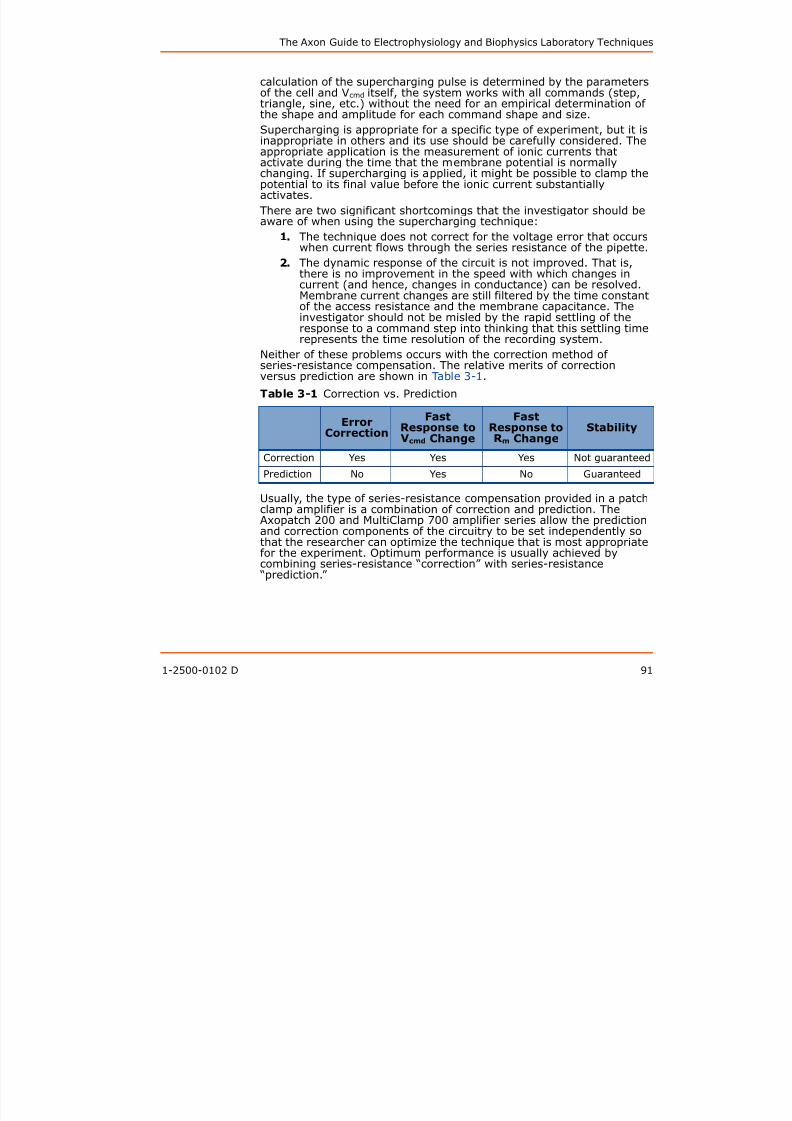
8/13/2019 User Guide v3
http://slidepdf.com/reader/full/user-guide-v3 92/302
1-2500-0102 D 91
activate during the time that the membrane potential is normallychanging. If supercharging is applied, it might be possible to clamp thepotential to its final value before the ionic current substantiallyactivates.
There are two significant shortcomings that the investigator should beaware of when using the supercharging technique:
1. The technique does not correct for the voltage error that occurswhen current flows through the series resistance of the pipette.
2. The dynamic response of the circuit is not improved. That is,there is no improvement in the speed with which changes incurrent (and hence, changes in conductance) can be resolved.Membrane current changes are still filtered by the time constantof the access resistance and the membrane capacitance. Theinvestigator should not be misled by the rapid settling of the
response to a command step into thinking that this settling timerepresents the time resolution of the recording system.
Neither of these problems occurs with the correction method ofseries-resistance compensation. The relative merits of correctionversus prediction are shown in Table 3-1.
Usually, the type of series-resistance compensation provided in a patchclamp amplifier is a combination of correction and prediction. TheAxopatch 200 and MultiClamp 700 amplifier series allow the predictionand correction components of the circuitry to be set independently so
that the researcher can optimize the technique that is most appropriatefor the experiment. Optimum performance is usually achieved bycombining series-resistance “correction” with series-resistance “prediction.”
Table 3-1 Correction vs. Prediction
Error
Correction
FastResponse to
Vcmd Change
FastResponse to
R m Change
Stability
Correction Yes Yes Yes Not guaranteed
Prediction No Yes No Guaranteed
Instrumentation for Measuring Bioelectric Signals from Cells
Limitations of Series-Resistance Compensation
Series-resistance compensation is an attempt to electronically reducethe effect of the pipette resistance. Because of practical limitations, it is
never perfect. Even if 100% compensation could be used with stability,this would only apply to DC and medium-speed currents. Very fastcurrents cannot be fully corrected.
i i i
8/13/2019 User Guide v3
http://slidepdf.com/reader/full/user-guide-v3 93/302
92 1-2500-0102 D
Pipette-Capacitance Compensation
When the command voltage is stepped, a large amount of current flowsinto the pipette capacitance during the transition from one potential tothe next. In an intracellular micropipette amplifier, such as theAxoclamp 900A amplifier, this is reduced by setting the capacitance
neutralization controls, as discussed in the earlier section titledCapacitance Compensation. In a patch-clamp amplifier, such as theAxopatch 200 and MultiClamp 700 amplifier series, a variation of thetechnique is used for the same purpose—to reduce or even eliminatethe transient. This section discusses pipette capacitance compensationin a patch clamp.
Compensating the pipette capacitance in a patch clamp has threepurposes. First, many researchers want to remove the transient fromthe records for “cosmetic” reasons. Second, during the transient the
potential at the top of the pipette is changing slowly while the pipettecapacitance charges. By rapidly charging the pipette capacitancethrough the compensation circuitry, the potential at the top of thepipette is stepped more rapidly, reducing the likelihood that rapid-onsetionic currents will be distorted. Third, uncompensated pipettecapacitance has a detrimental effect on the stability of the series-resistance correction circuitry. The component of the current that flowsinto the pipette capacitance is not in series with any resistance. Thusthe series-resistance correction circuit exceeds 100% compensation for
this component of the current as soon as the circuit is switched in.In the Axopatch and MultiClamp amplifiers, two pairs of pipettecapacitance compensation controls are available. With these controls, itis often possible to reduce the pipette transients to extremely lowlevels. The bulk of the transient is reduced by using the fast magnitudeand time constant (τ) controls. The magnitude control compensatesthe net charge. The τ control adjusts the time constant of the chargecompensation to match the time constant of the command pathway andto compensate for small non-idealities in the frequency response of the
pipette and electronics.The residual slow component seen in many pipettes is reduced by usingthe slow magnitude and τ controls. A simplified circuit of the fast andslow compensation circuitry is shown in Figure 3-18.

8/13/2019 User Guide v3
http://slidepdf.com/reader/full/user-guide-v3 94/302
Instrumentation for Measuring Bioelectric Signals from Cells
Whole-Cell Capacitance Compensation
When the membrane potential is stepped, there is a significant currenttransient required to charge the membrane capacitance. This is true
whether the cell is clamped using a two-electrode clamp or asingle-electrode clamp. Since it is impossible to record meaningfulcurrents during this transient (the membrane potential has not settled),this transient is ignored in most two-electrode voltage-clamp ordiscontinuous single-electrode voltage-clamp experiments However
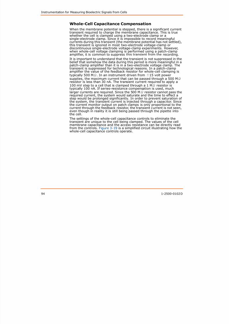
8/13/2019 User Guide v3
http://slidepdf.com/reader/full/user-guide-v3 95/302
94 1-2500-0102 D
discontinuous single-electrode voltage-clamp experiments. However,when whole-cell voltage clamping is performed using a patch-clampamplifier, it is common to suppress this transient from the recording.
It is important to understand that the transient is not suppressed in thebelief that somehow the data during this period is more meaningful in a
patch-clamp amplifier than it is in a two-electrode voltage clamp. Thetransient is suppressed for technological reasons. In a patch-clampamplifier the value of the feedback resistor for whole-cell clamping istypically 500 MΩ. In an instrument driven from ±15 volt powersupplies, the maximum current that can be passed through a 500 MΩresistor is less than 30 nA. The transient current required to apply a100 mV step to a cell that is clamped through a 1 MΩ resistor istypically 100 nA. If series-resistance compensation is used, muchlarger currents are required. Since the 500 MΩ resistor cannot pass the
required current, the system would saturate and the time to effect astep would be prolonged significantly. In order to prevent saturation ofthe system, the transient current is injected through a capacitor. Sincethe current monitor output on patch clamps is only proportional to thecurrent through the feedback resistor, the transient current is not seen,even though in reality it is still being passed through the pipette intothe cell.
The settings of the whole-cell capacitance controls to eliminate thetransient are unique to the cell being clamped. The values of the cell
membrane capacitance and the access resistance can be directly readfrom the controls. Figure 3-19 is a simplified circuit illustrating how thewhole-cell capacitance controls operate.
The Axon Guide to Electrophysiology and Biophysics Laboratory Techniques
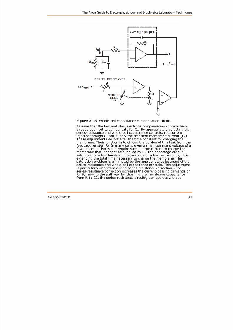
8/13/2019 User Guide v3
http://slidepdf.com/reader/full/user-guide-v3 96/302
1-2500-0102 D 95
Figure 3-19 Whole-cell capacitance compensation circuit.
Assume that the fast and slow electrode compensation controls have
already been set to compensate for Cp. By appropriately adjusting theseries-resistance and whole-cell capacitance controls, the currentinjected through C2 will supply the transient membrane current (Im).These adjustments do not alter the time constant for charging themembrane. Their function is to offload the burden of this task from thefeedback resistor, Rf . In many cells, even a small command voltage of afew tens of millivolts can require such a large current to charge themembrane that it cannot be supplied by Rf . The headstage outputsaturates for a few hundred microseconds or a few milliseconds, thus
extending the total time necessary to charge the membrane. Thissaturation problem is eliminated by the appropriate adjustment of theseries-resistance and whole-cell capacitance controls. This adjustmentis particularly important during series-resistance correction sinceseries-resistance correction increases the current-passing demands onRf . By moving the pathway for charging the membrane capacitancefrom Rf to C2, the series-resistance circuitry can operate without

8/13/2019 User Guide v3
http://slidepdf.com/reader/full/user-guide-v3 97/302
The Axon Guide to Electrophysiology and Biophysics Laboratory Techniques
Absolute Value
The absolute value of the membrane capacitance is displayed on thewhole-cell capacitance dial after the whole-cell current transient has
been eliminated. This value may be used to estimate the surface areaof the cell assuming that the membrane capacitance per unit area is1 μF/cm2.
Rupturing the Patch

8/13/2019 User Guide v3
http://slidepdf.com/reader/full/user-guide-v3 98/302
1-2500-0102 D 97
Rupturing the Patch
To go from the patch to the whole-cell mode, the usual method used torupture the membrane under the pipette is to apply a pulse of gentlesuction. This can be done by mouth or by syringe. “Zap” is anotheralternative for going whole-cell. In this technique, a large, brief
hyperpolarizing voltage pulse (about 1.5 V) is applied to the cell. Thispulse initiates dielectric breakdown of the membrane patch and allowsaccess to the interior of the cell. It is important to use the briefest pulseconsistent with low-access resistance. If the pulse is too long, the sealmight be lost. Both the Axopatch 200B and MultiClamp 700B amplifierallow the Zap pulse to be applied for 0.5 ms or less at the minimum.
With some cells it is difficult to go whole cell without losing the seal. Analternative is the perforated patch technique, which is discussed inChapter 5: Advanced Methods in Electrophysiology on page 129.
Which one Should you Use: dSEVC or cSEVC?
Two methods can be used to implement a whole-cell patch voltageclamp. The first is the discontinuous single-electrode voltage clamp(dSEVC) method. The second is the continuous single-electrode voltageclamp (cSEVC) method. The cSEVC method is more commonly knownas the “whole-cell patch clamp”; but formally, the term cSEVC is moredescriptive of the method. Both methods have their pros and cons. ThedSEVC is generally superior when the currents being clamped aremodest or large in size ( > 5 nA), leading to a concern that the errordue to the uncompensated series resistance might be significant. IndSEVC mode, if the sampling rate is correctly chosen and thecapacitance compensation correctly set, there is no error due to seriesresistance. For small currents, the dSEVC mode is less attractivebecause it is more difficult to set up and because it is noisier. Moreover,the error due to the uncompensated series resistance can generally bemade negligible for small currents, making the cSEVC mode veryattractive.
The cSEVC mode is available on patch-clamp amplifiers (Axopatch 200Band MultiClamp 700B) as the “whole-cell patch” mode. In a patch-clamp amplifier, the voltage-clamp circuit is a current-to-voltageconverter located in the headstage (described in detail below; seeFigure 3-21). The Axoclamp 900A amplifier offers the dSEVC mode,and the voltage-clamp circuit is located in the main unit. There arefewer ancillary controls in the Axoclamp 900A amplifiers pertaining towhole-cell patch clamp as compared to the Axopatch 200B and
Instrumentation for Measuring Bioelectric Signals from Cells
MultiClamp 700B amplifiers. For example, the Axoclamp 900A amplifierdoes not have a whole-cell capacitance compensation control.
Space Clamp Considerations
There is one limitation to the performance of the voltage clamp thatcannot be electrically compensated. This is the deviation of the cellfrom a sphere centered on the tip of the voltage-recordingmicropipette. The voltage clamp is maintained at the tip of the

8/13/2019 User Guide v3
http://slidepdf.com/reader/full/user-guide-v3 99/302
98 1-2500-0102 D
voltage-recording micropipette. If all portions of the cell membrane areseparated from this tip by equal access resistance, then the membranewill be uniformly voltage clamped. However, many cells have processessuch as axons, dendrites and filopodia attached to the cell body (wherethe micropipettes are usually located). The membranes of these
processes are separated from the cell body by an axial accessresistance whose value depends on the distance to each portion of themembrane and the cross section in that region of the cell. Thus there isa voltage drop across the access resistance that becomes substantialfor distal components of the membrane. Even though the somaticmembrane potential may be well controlled, the axonal or dendriticmembrane potential may be very poorly controlled. In these cases, thetime course of synaptic currents, regenerative currents andmeasurements of reversal potentials may be grossly distorted.
As a general rule, the voltage clamp is considered to be acceptable ifthe length of the attached axon or dendrites is no more than 1/10 ofthe length constants. Even this short length will cause significantdistortion of fast currents (see Figure 7 in Rall and Segev, 1985).Calculation of the length constant for a cell is complicated since itdepends on the geometry of the particular cell under investigation.Some of the common ways to avoid the problems of poor spaceclamping are as follows:
1. Restrict investigations to spherical cells. Many cultured cells are
convenient.2. Ligate attached axons. For example, the axon of large molluscan
neurons can be tied off with nylon thread.
3. Use short segments. For example, short segments (100 μm) ofarteriolar syncytia can be separated from the arteriole by carefulcutting with a razor blade.
4. Restrict the range of the clamp to a short segment of the cell.This is the essence of the “sucrose gap” technique sometimes
used on axons.5. Restrict the measurement to currents that are generated close
to the micropipettes. For example, the end plate currents inmuscle fibers can be well clamped, even though the bulkmembrane current is very poorly clamped.
6. Restrict the measurement to the current flowing through a largepatch of membrane instead of the whole cell. The “macro patch”
The Axon Guide to Electrophysiology and Biophysics Laboratory Techniques
technique is a special case of the single-channel patch-clamptechnique described in Chapter 5: Advanced Methods inElectrophysiology on page 129, in which there are sufficientchannels for an ensemble current to be recorded.
7. Apply the patch pipette not at the cell body, but out on theprocess. This technique has been successfully applied todendrites, for example, where electrical access to the cell isachieved far from the cell body along a dendritic shaft. Thisshould improve voltage clamp in nearby dendritic spines.

8/13/2019 User Guide v3
http://slidepdf.com/reader/full/user-guide-v3 100/302
1-2500-0102 D 99
should improve voltage clamp in nearby dendritic spines.
Single-Channel Patch Clamp5
The single-channel patch clamp is a special case of the voltage-clamptechnique. This technique permits the direct measurement of thedynamic activity of individual membrane-bound channel proteins.
Like the whole-cell patch technique, a blunt pipette is sealed onto apatch of membrane. If single-channel recording is intended, themembrane at the tip of the pipette is preserved (for example, notruptured). The current recorded is then simply the current that flowsthrough the membrane at the tip of the pipette. Since this membranearea is very small, there is a good chance that just one or a a few ionchannels are located in the patched membrane. Individual ion-channelcurrents can thus be recorded. Previously, the only way to estimatekinetics or conductance of these channels was the technique of “noise”or “fluctuation” analysis. Noise analysis yields an estimate of the meanlifetimes of the channels and the mean amplitudes, but no informationabout actual opening and closing transitions nor about the shape of theconductance changes.
In single-channel recording, the current through the series resistanceof the pipette is negligible, perhaps only a few picoamps flowing
through a series resistance of just 10 MΩ
. The resulting voltage error is just a few tens of microvolts and is always ignored.
The Importance of a Good Seal
When a heat-polished pipette is pressed against a cell membrane itmay adhere tightly. The interior of the pipette is then isolated from theextracellular solution by the seal that is formed. If the resistance of thisseal is infinite, no current can leak across it.
Current leakage though the seal resistance has a crucial bearing on thequality of the patch current recording. Firstly, depending on the size ofthe seal resistance, a fraction of the current passing through the
5. Parts of this section have been reprinted with permission from Finkel, A. S.,
Progress in Instrumentation Technology for Recording from Single Channels and
Small Cells, in Cellular and Molecular Neurobiology: A Practical Approach,
Oxford University Press, 1991.
Instrumentation for Measuring Bioelectric Signals from Cells
membrane patch will leak out through the seal and will not bemeasured. The lower the seal resistance the larger the fraction ofundetected current.
Secondly, thermal movement of the charges in the conducting
pathways of the seal constitute the major source of noise in therecording unless the seal resistance is very high (several gigohms ormore). A high seal resistance is a prerequisite of low-noise recordings.
High-resistance seals, often called “gigaseals,” require that very cleanpipettes be used and that they only be used once If this is the case

8/13/2019 User Guide v3
http://slidepdf.com/reader/full/user-guide-v3 101/302
100 1-2500-0102 D
pipettes be used and that they only be used once. If this is the case,gigaseals will routinely form after the application of gentle suction.When good gigaseals are formed, the noise due to the leakage currentis virtually eliminated and other sources of noise remain the dominantlimitations in the resolution of the recording technique. These are the
noise of the electronics, the pipette glass, the input capacitance and thefeedback resistor. Commercial patch clamp amplifiers such as theAxopatch 200B amplifier have minimized the noise of the electronicsand the feedback element in the headstage. Chapter 4: Microelectrodesand Micropipettes on page 117 describes the attributes of desirableglasses and the ways to fabricate low-noise pipettes. It also discussesthe use of Sylgard coatings to minimize pipette capacitance.
Resistor Feedback Technology
Current-to-Voltage Converter
The basic concept behind the design of patch-clamp electronics is verysimple Figure 3-21). A sensitive current-to-voltage converter isfabricated using a high-megohm resistor (Rf ) and an operationalamplifier (A1). The pipette is connected to the negative input and thecommand voltage is connected to the positive input. Since theoperational amplifier has extremely high gain, the potential at thenegative input is forced to follow the potential at the positive input. All
current flowing in the micropipette also flows through Rf. This current isproportional to the voltage across Rf which is measured at the output ofthe differential amplifier (A2).
The Axon Guide to Electrophysiology and Biophysics Laboratory Techniques

8/13/2019 User Guide v3
http://slidepdf.com/reader/full/user-guide-v3 102/302
1-2500-0102 D 101
Figure 3-21 Resistive headstage.
Operational amplifier A1 is configured as a current-to-voltageconverter. Differential amplifier A2 subtracts Vcmd from the output of A1to generate a voltage that is purely proportional to the voltage across Rf and hence the feedback current, If . The boost circuit increases the high-
frequency gain to compensate for the narrow bandwidth of thefeedback resistor.
In principle, the patch clamp is equivalent to a conventionaltwo-electrode voltage clamp in which the output circuit is connectedback to the input pipette. In practice, the patch clamp is betterbehaved. The patch-clamp system is simpler since all of the gain is in asingle operational amplifier stage. The stray capacitance across thefeedback resistor guarantees stability. Furthermore, because the gainof this operational amplifier is so high, the difference between the
command potential and the potential of the micropipette is negligible.Remember that the potential that is controlled is the potential at thetop of the micropipette, not the potential at its tip.
Problems
The special demands of patch clamping lead to complicating factors inthe design of a good headstage.
1. Integrated circuit operational amplifiers do not have therequired combination of ultra-low noise and sub-picoamp biascurrents. Thus the operational amplifier has to be made from acomposite of low-noise FETs6, such as the U430 type, andconventional operational amplifiers. The voltage noise of theinput FETs leads to noise current being injected into the inputcapacitance. If this input capacitance is large, this source ofnoise becomes dominant; it is proportional to the product of theinput capacitance and the noise of the input FETs.
Instrumentation for Measuring Bioelectric Signals from Cells
2. The minimum theoretically achievable current noise is lower forlarger Rf values; therefore it is important to choose large Rfvalues. The largest value typically used is 50 GΩ, since it allowsa reasonable maximum current of more than 200 pA to be
measured. Unfortunately, for reasons that are not wellunderstood, high-value resistors are several times noisier thanpredicted by thermal-noise theory. Since the noise of theseresistors cannot be predicted, various brands of resistors mustbe tested until the best one is found.

8/13/2019 User Guide v3
http://slidepdf.com/reader/full/user-guide-v3 103/302
102 1-2500-0102 D
3. The inherent bandwidth of a 50 GΩ resistor is limited by thestray capacitance across the resistor (CRf in Figure 3-21). Forexample, a 50 GΩ resistor with 0.1 pF stray capacitance has a5 ms time constant, corresponding to a bandwidth of only
32 Hz. This poor time resolution is unacceptable for measuringionic currents. Therefore, the high-frequency components of theheadstage output signal must be boosted. This is typicallyachieved by an analog frequency compensation circuit. Thiscircuit is made complicated by the fact that Rf cannot beconsidered as an ideal capacitor in parallel with an ideal resistor;thus a simple high-pass filter cannot be used. Complex circuitsconsisting of up to four poles and three zeros in the transferfunction are commonly used. The placement of the poles andzeros must be carefully set for the particular resistor.
4. The current required to charge the input capacitance during astep voltage command can easily exceed the maximum currentthat can be passed by Rf from the typical 13 V swing of theoperational amplifier. For example, to linearly charge 5 pF ofinput capacitance to 100 mV in 10 μs would require a chargingcurrent of 50 nA. This is well beyond the 260 pA that can bepassed by a 50 GΩ resistor driven from ±13 V. Thus, specialcircuits are typically added to inject the required charging
current through a capacitor.5. The best high-value resistors seem to be available only in aminiature “surface mount” form. This means that the headstageelectronics have to be manufactured in a hybrid. Thismanufacturing technique has some advantages. First, the U430input FETs and other FETs typically used to switch betweendifferent values of Rf can be used in an unpackaged form. This isto be preferred, since the sealing glasses used in packagedtransistors typically have a leakage resistance that increases thenoise. Second, it means that the sensitive input components canbe maintained in a hermetically sealed environment thatreduces the rate at which they age due to environmentalcontamination.
The Axon Guide to Electrophysiology and Biophysics Laboratory Techniques
If the Probe Output is Slow, How Can Voltage Clamping beFast?
In resistive-feedback headstages (but not capacitive-feedback
headstages, discussed below) the current output of thecurrent-to-voltage (I-V) converter in the probe is slow. Thehigh-frequency boost occurs afterwards and cannot influence theevents at the pipette. Thus, one might conclude that the voltage clampof the pipette must also be slow.
In fact despite the slow current output of the I V converter the voltage

8/13/2019 User Guide v3
http://slidepdf.com/reader/full/user-guide-v3 104/302
1-2500-0102 D 103
In fact, despite the slow current output of the I-V converter, the voltageclamp of the pipette is rapid. The pipette is connected to the negativeinput (summing junction) of the op amp. The command potential isconnected to the positive input of the op amp. The operation of the op
amp in this configuration is to force the potential at the summing junction to rapidly follow the potential at the positive input. If thecommand potential is a step, the potential at the summing junction(and hence the pipette) is also a step. The current required to achievethis step is passed through the feedback resistor (Rf ) and theassociated stray feedback capacitance (CRf ) of the I-V converter. Theoutput of the I-V converter settles to the final value with time constantRf CRf . This relatively slow settling occurs despite the fact that the stepat the summing junction is fast.
In this discussion, we have carefully referred to the fact that it is thepipette that is rapidly voltage clamped. The membrane potential isvoltage clamped to its final value much more slowly. To a reasonableapproximation, the time constant for voltage clamping the membrane isRpCm, where Rp is the pipette resistance and Cm is the membranecapacitance.
Capacitor Feedback Technology
Rationale
A newer technology in single-channel recording is thecapacitor-feedback technique, also known as the integrating headstagetechnique. While this technique was talked about for many years, it wasonly first attempted and described in 1985 by Offner and Clark.Practical implementations did not become commercially available until1989.
In this technique, the feedback resistor in the headstage is replaced bya capacitor (Cf in Figure 3-22). When a capacitor is used instead of a
resistor, the headstage acts as an integrator. That is, for a constantinput current, the output of the headstage is a ramp. The slope of theramp is proportional to the current. To recover a voltage that is simplyproportional to the input current, the integrator must be followed by adifferentiator (A2).
Instrumentation for Measuring Bioelectric Signals from Cells

8/13/2019 User Guide v3
http://slidepdf.com/reader/full/user-guide-v3 105/302
104 1-2500-0102 D
Figure 3-22 Capacitive feedback headstage.
The feedback element around operational amplifier A1 is capacitor (Cf ).Thus the output of A1 is the integral of the pipette current. The actualcurrent is recovered from the integral by differentiating it in thedifferentiator formed by Cd, Rd and A2.
Compared with resistor-feedback picoamp current-to-voltage
converters (RIV), capacitor feedback current-to-voltage converters(CIV) exhibit less noise, increased dynamic range, wider bandwidth,and improved linearity.
Noise, Dynamic Range, Linearity, and Bandwidth
1. The noise of the CIV is lower for two reasons. First, thecapacitors do not generate as much thermal noise as resistorsdo. (There is an equivalent resistor noise source due to thedifferentiator, but with careful design this can be made
negligible.) Second, capacitors are commercially available thatare free of the excess noise sources that plague high-gigaohmresistors.
The noise benefit of the CIV is eliminated if Cf is large (10 pF ormore). This is because from the noise point of view, Cf sumswith the other sources of input capacitance. The voltage noise ofthe input FETs leads to a current injection into the total inputcapacitance. If this input capacitance is large, this source ofnoise becomes dominant.
The lower noise of the CIV can be realized only in situationswhere all other noise sources are minimized. That is, theexperimenter should use a low-noise glass and pipette holder,Sylgard coating, and a high-resistance seal. By carefullyremoving other sources of noise, the reduced noise of the CIVcan be realized in real patches, not just in theory.
The Axon Guide to Electrophysiology and Biophysics Laboratory Techniques
2. The capacitor-feedback headstage has an equivalent transferresistance (RT) given by
Because the noise is theoretically independent of the Cf valueand the gain of the differentiator, RT, may be kept quite low, forexample, 100 MΩ. At this gain, the maximum current that can

8/13/2019 User Guide v3
http://slidepdf.com/reader/full/user-guide-v3 106/302
1-2500-0102 D 105
example, 100 MΩ. At this gain, the maximum current that canbe recorded is 500 times greater than for an RIV using a 50 GΩ feedback resistor. Thus the CIV potentially has vastly improveddynamic range.
3. In the section on Resistor Feedback Technology, it was pointedout that in order to achieve an acceptable bandwidth of, forexample, 20 kHz for single-channel recording, a complex boostcircuit has to be used to correct the frequency response. Even ifthe boost box has as many as four poles and three zeros, thefrequency response of Rf is not perfectly corrected. Theimperfections of the correction are most easily seen byobserving the step response of the headstage. Frequently, therewill be overshoots and ripples that can amount to as much as
2% of the response. However, because excellent capacitors areavailable, the step response is inherently square with a CIV.
4. The bandwidth of a CIV can be very wide. It is maximized byusing a small value of Cf and a small value of Rd. For practicalvalues (Cf = 1 pF and Rd = 150 kΩ), the bandwidth is of theorder of 70 kHz or more. This is considerably better than the20 kHz of a good RIV using a 50 GΩ feedback resistor.
Whether it is practical to use this increased bandwidth or not isanother matter. The noise of both the RIV and the CIV
headstages increases dramatically with frequency.
Problems
There are two major problems that make the capacitor feedbacktechnology difficult to implement. The first problem is that after asustained net DC input current the integrator voltage ramps towardsone of the power-supply limits. When this happens, the integrator mustbe reset by discharging the capacitor. The frequency of the resetsdepends on the size of Cf and the average input current. For example, if
Cf is 1 pF and the input current is 2 pA, the output of the integrator willramp at 2 V/s. If the resetting circuitry is triggered when the integratorvoltage exceeds 10 V, resets will occur every five seconds.
The reset itself lasts approximately 50 μs. During the reset,sample and-hold circuits are used to maintain the current output at itsvalue immediately prior to the start of the reset. If it is acceptable tolose 0.1% of the data, resets as frequent as every 50 ms would be
Instrumentation for Measuring Bioelectric Signals from Cells
acceptable. In the above example, this corresponds to an input currentof 200 pA. For single-channel recording, this is more than adequate.
Figure 3-23 shows the signal pathway for the capacitor-feedbackheadstage. The output current (I) of the capacitor-feedback headstage
is normally connected through a switch to the output pre-filteramplifier, then to the low-pass filter, and finally to the post-filteramplifier. The signal also goes through a low-pass filter to asample-and-hold amplifier. During reset, the switch shifts to the RESETposition. Simultaneously, the sample-and-hold amplifier is switched tothe hold mode so that the signal immediately before the reset transient

8/13/2019 User Guide v3
http://slidepdf.com/reader/full/user-guide-v3 107/302
106 1-2500-0102 D
g yoccurs is presented to the output amplifiers.
Figure 3-23 Signal handling during resets in the capacitor-feedbackheadstage.
A capacitor feedback is not practical for whole-cell recordings. Due tothe large whole-cell currents the resets would be too frequent unlessthe value of Cf was increased. In practice, it is hardly worth it. It issimpler to switch to a modest-sized resistor (for example, 500 MΩ) andavoid the problem of resets altogether. Reverting to resistor-feedbackmethods for wholecell recordings does not represent a setback in termsof noise because the 500 MΩ resistor is not the dominant source ofnoise.
During the measurement of voltage-activated single-channel currents,the resets can be made irrelevant. This is done by using a control pulseto force a reset immediately prior to the voltage step. This guaranteesthat Cf is in its discharged state at the beginning of the voltage step andis therefore unlikely to need resetting during the step.
The second problem is that during resets transients are injected intothe headstage input by the reset circuitry. If left uncompensated, these
would cause unwanted and possibly damaging current pulses to beinjected down the micropipette into the patch. Special compensationcircuitry needs to be included in the design to exactly balance out these
injected currents.
There are other transient problems that occur during and after thereset. These include dielectric absorption in the differentiator andfeedback capacitors, and other ill-defined transients that work their
The Axon Guide to Electrophysiology and Biophysics Laboratory Techniques
way into the system. Compensation circuitry must also be included tocompensate for these transients.
Overall, the need to reset and to compensate for the many transientsthat occur during reset make the design of an integrating patch clamp
challenging. However, in a well-designed system, the reset transientsmeasured at the output will be less than 1 pA measured in a 1 kHzbandwidth.
Special Considerations for Bilayer Experiments

8/13/2019 User Guide v3
http://slidepdf.com/reader/full/user-guide-v3 108/302
1-2500-0102 D 107
The Advantage of Resets in Bilayer Experiments
While they are normally considered to be a nuisance, there is one
application where resets are quite an advantage. This is in voltage-stepexperiments in bilayers. During a reset, a low resistance of about10 kΩ is placed in parallel to the feedback capacitor. This resistorallows currents up to 1 mA to pass out of the headstage to rapidlycharge the bilayer capacitance. Voltage steps as large as 100 mV arenormally achieved with one or two resets separated by less than amillisecond.
Noise vs. Access Resistance
In bilayer experiments, the access resistance is quite low, usuallyranging from a few kilohms to several tens of kilohms. The accessresistance is in series with the membrane capacitance and producesvoltage noise just as though the headstage had high intrinsic noise.
For bilayer recording done at a low bandwidth (<1 kHz), the enCin noisehas not yet become the major contributor to the overall noise (where en is the voltage noise of the probe input FETs and Cin is the capacitance atthe input of the headstage primarily due to the bilayer membranecapacitance). If the access resistance is large enough, it becomes the
dominant noise contributor at low bandwidths.Figure 3-24 shows the dependence of peak-to-peak noise on accessresistance in a 1 kHz bandwidth for a given bilayer membranecapacitance. It can be seen that the lower the access resistance, thelower the noise. It is therefore important that the patch-clampinstrument be capable of operating without oscillation even whenextremely small, or zero, access resistances are used. The CV-203BUheadstage for the Axopatch 200B amplifier and the CV-7B/BLheadstage for the MultiClamp 700B amplifier have been designed for
complete stability even with extremely low access resistances.
Instrumentation for Measuring Bioelectric Signals from Cells

8/13/2019 User Guide v3
http://slidepdf.com/reader/full/user-guide-v3 109/302
108 1-2500-0102 D
Figure 3-24 Typical current noise in bilayer experiments.
How Fast is “fast”?
The speed of the observed transitions of single-channel currents is thesame as the response time of the electronics. Whenever recordings aremade at wider bandwidths, the observed transition rates becomeshorter. It is not clear that we will ever be able to resolve the actualtransition time using electrical measurements (perhaps opticaltechniques will emerge to do the job); but the discovery of new lower
limits to the transition rate will be made possible by the low-noisewide-bandwidth patch clamps such as the Axopatch 200 seriesamplifiers.
Measurement of Changes in Membrane Capacitance
The measurement of minute changes in membrane capacitance, suchas the changes that occur during exocytosis, was made practical by thewhole-cell patch-clamp technique. Two methods can be used. The
simplest and the most traditional way is to use a fitting technique tofind the time constant of the current response to a voltage step. Byassuming a simple cell model, the membrane capacitance can be easilydeduced. This technique is relatively easy to apply, but it has aresolution no better than 100–200 fF, which is insufficient to resolve the10–20 fF capacitance increases occurring during fusion of singlegranules with the membrane.

8/13/2019 User Guide v3
http://slidepdf.com/reader/full/user-guide-v3 110/302
Instrumentation for Measuring Bioelectric Signals from Cells
Micropipette Holders
High-quality micropipette holders are crucial to successfulsingle-channel recording. Two characteristics of the holder areimportant. First, the holder must be mechanically stable. When workingwith a cell-attached patch, drift of the micropipette is unacceptable.Clearly, a low-drift micromanipulator is required (as discussed inChapter 2: The Laboratory Setup on page 39). But if the holder is loosein the headstage connector or if the pipette does not seat properly, driftwill occur despite the high quality of the micromanipulator. Onecommon, exasperating problem associated with loose holders is
8/13/2019 User Guide v3
http://slidepdf.com/reader/full/user-guide-v3 111/302
110 1-2500-0102 D
common, exasperating problem associated with loose holders ismovement of the pipette when suction is applied, which either preventsseal formation or damages the cell. The HL-U holders from MolecularDevices fit all recent Axon Conventional Electrophysiology headstages
and have been designed to fit snugly into the headstage connector andto firmly grip the pipette to prevent drift. Second, the holder must notintroduce noise. To assure this:
1. Select the right holder material. When a holder is connected tothe headstage, even before a pipette is connected, the open-circuit noise goes up slightly. The reasons are not understood.Empirical tests have shown that when used with glassmicropipettes, polycarbonate adds the least noise. The HL-Uholders use polycarbonate for the pipette cap and the body of
the holder. The portion that plugs into the headstage is made ofTeflon. Teflon in this position does not add noise, and itfacilitates smooth insertion and removal.
2. Use a small pin for the electrical connection. Large pins havemore capacitance contributed by the surrounding groundedsurfaces.
3. Do not use a shield. Surrounding the holder with a driven orgrounded shield adds to the input capacitance and thusincreases the noise.
Current Conventions and Voltage Conventions
The terminology used in this discussion applies to all Axon ConventionalElectrophysiology amplifiers manufactured by Molecular Devices.
Definitions
Positive Current
The flow of positive ions out of the headstage into the microelectrodeand out of the microelectrode tip into the preparation is termed positivecurrent.
The Axon Guide to Electrophysiology and Biophysics Laboratory Techniques
Inward Current
Current that flows across the membrane, from the outside surface tothe inside surface, is termed inward current.
Outward CurrentCurrent that flows across the membrane, from the inside surface to theoutside surface, is termed outward current.
Positive Potential
Th i i i l i i l h h d
8/13/2019 User Guide v3
http://slidepdf.com/reader/full/user-guide-v3 112/302
1-2500-0102 D 111
The term positive potential means a positive voltage at the headstageinput with respect to ground.
Transmembrane PotentialThe transmembrane potential (Vm) is the potential at the inside of thecell minus the potential at the outside. This term is applied equally tothe whole-cell membrane and to membrane patches.
Depolarizing / Hyperpolarizing
The resting Vm value of most cells is negative. If a positive current flowsinto the cell, Vm initially becomes less negative. For example, Vm might
shift from an initial resting value of -70 mV to a new value of -20 mV.Since the absolute magnitude of Vm is smaller, the current is said todepolarize the cell (for example, it reduces the “polarizing” voltageacross the membrane). This convention is adhered to even if thecurrent is so large that the absolute magnitude of Vm becomes larger.For example, a current that causes Vm to shift from -70 mV to +90 mVis still said to depolarize the cell. Stated simply, depolarization is apositive shift in Vm. Conversely, hyperpolarization is a negative shift inVm.
Whole-Cell Voltage and Current Clamp
Depolarizing / Hyperpolarizing Commands
In whole-cell voltage clamping, whether it is performed by TEVC,dSEVC, cSEVC or whole-cell patch clamp, a positive shift in thecommand voltage causes a positive shift in Vm and is said to bedepolarizing. A negative shift in the command voltage causes anegative shift in Vm and is said to be hyperpolarizing.
Transmembrane Potential vs. Command Potential
In whole-cell voltage clamping, the command potential controls thevoltage at the tip of the intracellular voltage-recording microelectrode.The transmembrane potential is thus equal to the command potential.
Instrumentation for Measuring Bioelectric Signals from Cells
Inward / Outward Current
In a cell generating an action potential, depolarization is caused by aflow of positive sodium or calcium ions into the cell. That is,depolarization in this case is caused by an inward current.
During intracellular current clamping, a depolarizing current is apositive current out of the micropipette tip into the interior of the cell.This current then passes through the membrane out of the cell into thebathing solution. Thus, in intracellular current clamping, a depolarizing(positive) current is an outward current.
An inward sodium current flows in some cells after a depolarizing

8/13/2019 User Guide v3
http://slidepdf.com/reader/full/user-guide-v3 113/302
112 1-2500-0102 D
An inward sodium current flows in some cells after a depolarizingvoltage step. When the cell is voltage clamped, the sodium current iscanceled by an equal and opposite current flowing into the headstage
via the microelectrode. Thus it is a negative current. Whentwo-electrode voltage clamping was first used in the early 1950’s, theinvestigators chose to call the negative current that they measured adepolarizing current because it corresponded to the depolarizingsodium current. This choice, while based on sound logic, wasunfortunate because it means that from the recording instrument’spoint of view, a negative current is hyperpolarizing in intracellularcurrent-clamp experiments but depolarizing in voltage-clampexperiments.
To prevent confusion, Axon Conventional Electrophysiology instrumentsalways use current and voltage conventions based on the instrument’sperspective. That is, the current is always unambiguously defined withrespect to the direction of flow into or out of the headstage. Someinstrument designers have put switches into the instruments to reversethe current and even the command voltage polarities so that theresearcher can switch the polarities depending on the type ofexperiment. This approach has been rejected by Molecular Devicesbecause of the real danger that if the researcher forgets to move theswitch to the preferred position, the data recorded on the computer
could be wrongly interpreted. Molecular Devices believes that the datashould be recorded unambiguously.
Patch Clamp
By design, the patch-clamp command voltage is positive if it increasesthe potential inside the micropipette. Whether it is hyperpolarizing ordepolarizing depends upon whether the patch is “cell attached,” “insideout” or “outside out.” The patch-clamp pipette current is positive if itflows from the headstage through the tip of the micropipette into thepatch membrane.
Cell-Attached Patch
The membrane patch is attached to the cell. The pipette is connected tothe outside surface of the membrane. A positive command voltagecauses the transmembrane potential to become more negative,
The Axon Guide to Electrophysiology and Biophysics Laboratory Techniques
therefore it is hyperpolarizing. For example, if the intracellular potentialis -70 mV with respect to 0 mV outside, the potential across the patchis also -70 mV. If the potential inside the pipette is then increased from0 mV to +20 mV, the transmembrane potential of the patchhyperpolarizes from -70 mV to -90 mV.
From the examples it can be seen that the transmembrane patchpotential is inversely proportional to the command potential, andshifted by the resting membrane potential (RMP) of the cell. A positivepipette current flows through the pipette across the patch membraneinto the cell. Therefore a positive current is inward.
I id O t P t h

8/13/2019 User Guide v3
http://slidepdf.com/reader/full/user-guide-v3 114/302
1-2500-0102 D 113
Inside-Out Patch
The membrane patch is detached from the cell. The surface that was
originally the inside surface is exposed to the bath solution. Now thepotential on the inside surface is 0 mV (bath potential). The pipette isstill connected to the outside surface of the membrane. A positivecommand voltage causes the transmembrane potential to becomemore negative, therefore it is hyperpolarizing. For example, toapproximate resting membrane conditions of Vm = -70 mV, thepotential inside the pipette must be adjusted to +70 mV. If thepotential inside the pipette is increased from +70 mV to +90 mV, thetransmembrane potential of the patch hyperpolarizes from -70 mV to-90 mV.
From the example it can be seen that the transmembrane patchpotential is inversely proportional to the command potential. A positivepipette current flows through the pipette across the patch membranefrom the outside surface to the inside surface. Therefore a positivecurrent is inward.
Outside-Out Patch
The membrane patch is detached from the cell in such a way that the
surface that was originally the outside surface remains exposed to thebath solution. The potential on the outside surface is 0 mV (bathpotential). The pipette interior is connected to what was originally theinside surface of the membrane. A positive command voltage causesthe transmembrane potential to become less negative, therefore it isdepolarizing. For example, to approximate resting membraneconditions, assuming that Vm = -70 mV, the potential inside the pipettemust be adjusted to -70 mV. If the potential inside the pipette
is then increased from -70 mV to -50 mV, the transmembrane potential
of the patch depolarizes from -70 mV to -50 mV.The membrane potential is directly proportional to the commandpotential. A positive pipette current flows through the pipette acrossthe patch membrane from the inside surface to the outside surface.Therefore a positive current is outward.
Instrumentation for Measuring Bioelectric Signals from Cells
Summary
1. Positive current corresponds to:
Cell-attached patch patch inward current
Inside-out patch patch inward currentOutside-out patch patch outward current
Whole-cell voltage clamp outward membrane current
Whole-cell current clamp outward membrane current
2. A positive shift in the command potential is:

8/13/2019 User Guide v3
http://slidepdf.com/reader/full/user-guide-v3 115/302
114 1-2500-0102 D
Cell-attached patch hyperpolarizing
Inside-out patch hyperpolarizing
Outside-out patch depolarizing
Whole-cell voltage clamp depolarizing
3. The correspondence between the command potential (Vcmd) andthe transmembrane potential (Vm) is:
Cell-attached patch Vm = RMP – Vcmd
Inside-out patch Vm = – Vcmd
Outside-out patch Vm = Vcmd
Whole-cell voltage clamp Vm = Vcmd
References
Patch Clamp
Rae, J.L. and Levis, R.A. Patch voltage clamp of lens epitheleal cells:theory and practice. Molec. Physiol, 6, 115–162, 1984.
Hamill, O. P., Marty, A., Neher, E., Sakmann, B., and Sigworth, F.J.Improved patchclamp techniques for high-resolution current recordingfrom cells and cell-free membrane patches. Pflugers Archiv., 391,85–100, 1981.
Sakmann, B. and Neher, E., Eds. Single-Channel Recording. New York:Plenum Press, 1983.
Joshi, C. & Fernandez, J. M. Capacitance measurements: an analysis ofthe phase detector technique used to study excocytosis and
endocytosis. Biophys. J. 53, 885–892, 1988.Finkel, A. S., Progress in instrumentation technology for recording fromsingle channels and small cells, in Cellular and Molecular Neurobiology:A Practical Approach. Oxford University Press, 1991.
The Axon Guide to Electrophysiology and Biophysics Laboratory Techniques
Two-Electrode Voltage Clamp
Finkel, A.S. & Gage, P.W. Conventional voltage clamping with twointracellular microelectrodes, in Voltage and Patch Clamping withMicroelectrodes. Ed. T. Smith Jr. et al., Baltimore: Williams & Wilkins,
1985.
Single-Electrode Voltage Clamp
Finkel, A.S. & Redman, S.J. Theory and operation of a singlemicroelectrode voltage clamp. J. Neurosci. Meths. 11, 101–127, 1984.

8/13/2019 User Guide v3
http://slidepdf.com/reader/full/user-guide-v3 116/302
1-2500-0102 D 115
Space-Clamp Considerations
Rall, W. & Segev, I. Space-clamp problems when voltage clampingbranched neurons with intracellular microelectrodes. in Voltage andPatch Clamping with Microelectrodes. Eds. T. Smith Jr. et al., Baltimore:Williams & Wilkins, 1985.
Other
Hille, B. Ionic Channels of Excitable Membranes. Sunderland,Massachusetts: Sinauer Associates. 1984.
Instrumentation for Measuring Bioelectric Signals from Cells

8/13/2019 User Guide v3
http://slidepdf.com/reader/full/user-guide-v3 117/302
116 1-2500-0102 D
4Microelectrodes and Micropipettes
Electrodes, Microelectrodes, Pipettes, Micropipettes, and
Pipette Solutions1
Electrodes convert ionic current in solution into electron current inwires; they are made of materials that can participate in a reversiblereaction with one of the ions in the solution. The most frequently used

8/13/2019 User Guide v3
http://slidepdf.com/reader/full/user-guide-v3 118/302
1-2500-0102 D 117
reaction with one of the ions in the solution. The most frequently usedelectrode material in electrophysiology is a silver (Ag) wire coated witha composite of Ag and silver-chloride (AgCl). For this electrode, chloride
ions (C1-) react with the Ag to produce AgCl plus an electron (e-), or anelectron reacts with AgCl to produce Ag plus Cl-. Thus, the currentcarried by chloride ions in the solution is converted into electronsaccording to the following reversible reaction:
The electrical potential at one of these electrodes is equal to thestandard electrochemical potential for Ag/AgCl plus RT/F ln(aCl-),
where R is the gas constant (8.314 V C K-1
mol-1
), T is the absolutetemperature on the Kelvin scale, F is Faraday’s constant (9.648 x 10⁴ C mol-1), and aCl- is the activity (for example, the effectiveconcentration) of Cl- in solution near the electrode solution interface.The potential difference between a pair of these electrodes should bezero if they are immersed in connected compartments with equalchloride concentrations. These concentrations must be kept constantduring the course of an experiment or an offset voltage will occur. Anoffset may be encountered when a Ag/AgCl electrode is used as a bathelectrode and the bath Cl- concentration is changed. To prevent this
type of voltage offset, many investigators connect their bath electrodethrough an agar bridge that maintains a constant Cl- concentration inthe immediate vicinity of the Ag/AgCl electrode.
Intracellular and patch microelectrodes contain a AgCl-coated Ag wireplaced in a solution-filled glass micropipette. The electrolyte solutionprovides the fluid connection from the cell to the electrode. Thus, theglass “electrodes” one pulls are not electrodes at all but simple conduitsof proper geometry to establish this fluid bridge. In recognition of this,microelectrodes are often referred to as “pipettes” or “micropipettes.”
The composition of the pipette solution depends on the type ofmeasurement being made. Standard intracellular microelectrodes thatare used to penetrate the cell membrane must be filled with a highly
1. Please see footnote 1 in Chapter 3: Instrumentation for Measuring Bioelectric
Signals from Cells on page 49.
Microelectrodes and Micropipettes
concentrated electrolyte solution, usually 2–4 M salt. The highelectrolyte concentration reduces the electrode resistance. Thisminimizes the rectifying current flow, lowers voltage noise and providesa wider recording bandwidth. A solution this concentrated dominatesthe liquid junction potential formed between the pipette solution andthe cell cytoplasm and results in a final junction potential that dependsprimarily on the relative mobilities of the anions and cations in thefilling solution. This is important for the measurement of DC voltagesbecause the cytoplasm anions are, predominantly, low mobility ions(mostly negative charges on large proteins), whereas the cations aresmall, high-mobility charges. The difference in the mobilities of thecellular anions and cations may result in a positive liquid junction
t ti l Thi iti li id j ti t ti l ld l d t th

8/13/2019 User Guide v3
http://slidepdf.com/reader/full/user-guide-v3 119/302
118 1-2500-0102 D
potential. This positive liquid junction potential would lead to themeasurement of an artificially depolarized membrane resting potential.
The concentrated pipette solution is important because it negates thedevelopment of the liquid junction potential, thus preventing anerroneous measurement of the resting potential. However, there is adisadvantage in using the concentrated filling solution since it can enterthe cell and produce a hyperosmotic load that would cause the cell toswell and alter its normal anion and cation content. While pipettes withvery small tip diameters can minimize or prevent concentrated solutionfrom entering the cell, they do so at the expense of noise, diminishingcurrent passing ability, and limiting recording bandwidth. Theselimitations result from the high resistance of small-tip pipettes. Inpractice, the choice of the pipette tip size reflects a compromisebetween its ability to prevent the concentrated solution from enteringthe cell and the pipette’s resistance.
Patch micropipettes are usually filled with a solution that is iso-osmoticto cell cytoplasm to allow current measurements in the absence of bulkwater flow. Because of the much larger diameter of the patch pipettetip (1–2 μm) as compared to the tip diameter of an intracellularmicroelectrode (0.01–0.1 μm), the lower ionic-strength filling solutionresults in an electrode whose resistance is as low as a few megohms.
The specific choice of the filling solution is dictated by the specificexperiment to be done. Care must be taken to minimize junction-potential artifacts. When the pipette tip is immersed in thebath, a junction potential is generated. Its magnitude depends on theconcentrations and mobilities of the ions in both the pipette solutionand the bath (see discussions of the Henderson equation inelectrochemistry textbooks). The junction potential is usually nulledwhile the pipette tip is immersed in the bath. When the seal forms, the junction potential disappears or changes its magnitude, and,
consequently, the nulling voltage is no longer correct. The junctionpotential also changes upon going whole cell. These effects must betaken into account or offset errors will exist in either single-channel orwhole-cell current recordings.
The filling solution in a patch pipette can be changed during the courseof an experiment by inserting a fine tube into the back of the pipettethrough a special post in the electrode holder. Different solutions can be

8/13/2019 User Guide v3
http://slidepdf.com/reader/full/user-guide-v3 120/302
Microelectrodes and Micropipettes
If not pre-cleaned, the glass tubing should be cleaned prior to thepreparation of the patch pipette. Sonicating the glass in 100% ethanolin an ultrasonic cleaner is an effective cleaning procedure. Aftercleaning, the glass should be placed in an oven at 200°C for 10–30minutes to achieve complete drying. This heat treatment is necessary
for low-noise recording in environments with very high humidity.Patch pipettes require much blunter tips than standard intracellularmicropipettes and it is usually impossible to pull them adequately onsingle-stage electrode pullers. Many laboratories have modifiedstandard vertical pipette pullers to operate as multiple-stage pipettepullers. Pulling pipettes, however, has become remarkably easier withthe advent of microprocessor-driven microelectrode pullers like those
il bl f th S tt I t t C With th ll it i
8/13/2019 User Guide v3
http://slidepdf.com/reader/full/user-guide-v3 121/302
120 1-2500-0102 D
available from the Sutter Instrument Company. With these pullers, it ispossible to implement very complicated multistage pulls of glass
pipettes and to store the parameters required for the desired operationin the instrument’s memory.
For the lowest noise recordings, patch pipettes must be coated with ahydrophobic material to prevent the bathing solution from creeping upthe wall of the pipette and, thus, limit a substantial noise source. Acommonly used compound is Sylgard #184 from Dow Corning(Midland, MI). Coating the glass with Sylgard also improves theelectrical properties of the glass. After preparing the Sylgard solutionper the manufacturer’s instructions, it can be stored in the freezer in
small, well-capped centrifuge tubes for several weeks. When brought toroom temperature for use in painting electrodes, this freezer-storedSylgard will last for several hours before it begins to polymerize.Sylgard is painted on the pipette tip using a small utensil, such as apiece of capillary tubing pulled over flame to a reasonably fine tip.Sylgard painting can be done using the magnifications available withstandard dissecting microscopes. The pipette is coated to within 100μm or less from its tip. It is important that the Sylgard be directedaway from the tip by gravity at all times during the painting procedure.
Otherwise, it will flow into the tip and make firepolishing and/or sealingimpossible. After painting, Sylgard can be cured by holding the tip for5–10 seconds in the hot air stream coming from a standard heat gun ofthe type used in electronics fabrication.
To promote gigaohm seals and to reduce the possibility of tippenetration into the cell during seal formation, pipette tips should befirepolished. Firepolishing is accomplished by connecting to amicromanipulator a rod of inert material to which a short loop ofplatinum iridium wire has been fastened. The ends of this wire must be
soldered to two other pieces of wire that can be connected to a voltageor current source to allow current passing through the platinum wire.The platinum loop is generally bent into a very fine hairpin so that itcan be brought to within a few microns of the electrode tip under directobservation using a compound microscope. Magnifications of600x–1500x are required for adequate visibility. The platinum wire isusually coated with a glass, such as Pyrex or Corning #7056, toprevent sputtering. After positioning the electrode tip near the
The Axon Guide to Electrophysiology and Biophysics Laboratory Techniques
glass-coated wire, current is passed through the wire to heat it. Theamount of current required depends on the softening temperature ofthe glass from which the pipette is constructed. The hot platinum wireheats the electrode tip and causes sharp corners to round and roughsurfaces to smooth. This polishing is best done under direct observation
at a magnification of 600x–1500x.
Pipette Properties for Single-channel vs.Whole-Cell Recording
Whereas some properties of pipettes used for single-channel andh l ll di i il th ti ti l diff t

8/13/2019 User Guide v3
http://slidepdf.com/reader/full/user-guide-v3 122/302
1-2500-0102 D 121
whole-cell recordings are similar, other properties are entirely different.Most importantly, reducing the noise of the pipette is much more crucialin single-channel recording than in whole-cell recording. The dominantnoise source in whole-cell recording is the pipette resistance that is inseries with the capacitance of the entire cell. Hence, the noisecontribution of the pipette is not as important. However, in order toprovide sufficient bandwidth for whole-cell current recording and tolimit command voltage errors, the resistance of a pipette used inwhole-cell recording should not exceed a few megohms. Limiting thepipette resistance is not required in single-channel recording; nor doesa higher pipette resistance, up to several tens of megohms, result in a
significant increase in the noise (see Chapter 11: Noise inElectrophysiological Measurements on page 259 for further discussionof pipette noise). In either single-channel or whole-cell recording,capacitance currents following voltage steps must be sufficiently smalland simple in time course to allow the researcher to compensate themby simple circuitry in the patch-clamp amplifier. Additionally, whetherused for single-channel or whole-cell recording, pipettes must be madeof glasses that do not leach compounds from their walls since thesecompounds might alter the currents measured from a particularchannel.
Types of Glasses and Their Properties
Patch-clamp pipette glasses can be classified on the basis of thetemperature at which they soften, on the basis of their electricalproperties, or on the basis of their major chemical constituents. Manyof these properties are itemized in specifications provided by themanufacturers. Therefore, it is often possible to choose glasses that
should be effective for patch clamping just by considering theirspecifications. Table 4-1 lists the properties of a number of glasses thathave been used for patch clamping. Glasses are listed in increasingorder of loss factors.
Microelectrodes and Micropipettes
Table 4-1 Electrical And Thermal Properties of Different Glasses.
GlassLoss
Factor
Log10
Volume
Resistivity
DielectricConstant
SofteningTemp. °C
Description
7940 0.0038 11.8 3.8 1580 Quartz (fused silica)
1724 0.0066 13.8 6.6 926 Aluminosilicate
7070 25 11.2 4.1 — Low loss borosilicate
8161 0.50 12.0 8.3 604 High lead
Sylgard 0 581 13 0 2 9 #184 Coating compound

8/13/2019 User Guide v3
http://slidepdf.com/reader/full/user-guide-v3 123/302
122 1-2500-0102 D
Sylgard 0.581 13.0 2.9 — #184 Coating compound
7059 0.584 13.1 5.8 844 Barium-borosilicate7760 0.79 9.4 4.5 780 Borosilicate
7040 1.00 9.6 4.8 700 Kovar seal borosilicate
KG-12 1.00 9.9 6.7 632 High lead
1723 1.00 13.5 6.3 910 Aluminosilicate
0010 1.07 8.9 6.7 625 High lead
EN-1 1.30 9.0 5.1 716 Kovar seal borosilicate
7720 1.30 8.8 4.7 755 Tungsten seal borosilicate
7056 1.50 10.2 5.7 720 Kovar seal borosilicate
3320 1.50 8.6 4.9 780 Tungsten seal borosilicate
7050 1.60 8.8 4.9 705 Series seal borosilicate
KG-33 2.20 7.9 4.6 827 Kimax borosilicate
7740 2.60 8.1 5.1 820 Pyrex borosilicate
1720 2.70 11.4 7.2 915 Aluminosilicate
N-51A 3.70 7.2 5.9 785 Borosilicate
R-6 5.10 6.6 7.3 700 Soda lime
0080 6.50 6.4 7.2 695 Soda lime
Note: The electrical properties and the thermal properties of the
glasses are not necessarily related to each other. Note also thatSylgard has better electrical properties than most glasses shown inthe table. It is, therefore, not surprising that heavy Sylgard coating ofpipettes fabricated from many types of glasses improves theirelectrical properties.
The Axon Guide to Electrophysiology and Biophysics Laboratory Techniques
Table 4-2 shows the chemical constituents of many of the same glasseslisted in Table 4-1. This table may be useful in deciding which glassesare likely to contain leachable components that might affect channelcurrents.
Table 4-2 Chemical Compositions of Different Glasses.

8/13/2019 User Guide v3
http://slidepdf.com/reader/full/user-guide-v3 124/302
1-2500-0102 D 123
Microelectrodes and Micropipettes
Thermal Properties of Glasses
Glasses that soften at lower temperatures offer several advantagesover glasses that soften at higher temperatures when fabricatingpatch-clamp pipettes. First, they do not impose a burden on theheating filaments of microelectrode pullers. Since low-filament currentis required to pull these glasses, filaments rarely change theirproperties with extended use and do not require replacement evenafter one or two years of continued operation. Second, pipettes withextremely blunt tips can be more readily fabricated from these glassesthan from glasses with high softening temperatures. Blunt tips providethe lowest access resistance (Ra) for whole-cell recording. Furthermore,the blunt-tapered pipettes are less likely to penetrate into the cell when

8/13/2019 User Guide v3
http://slidepdf.com/reader/full/user-guide-v3 125/302
124 1-2500-0102 D
pressed against the cell membrane during seal formation.
High-lead glasses pull at the lowest temperatures and are remarkablyamenable to firepolishing. It is possible to pull pipettes at such a lowtemperature that their tips are broken and jagged, forming tip openingswith diameters in excess of 50 μm, and yet the pipettes are easilyfirepolished into usable patch pipettes. Although the resulting tips areexceedingly blunt, these pipettes are effective in forming a tight sealwith the cell even when the final pipette resistance is < 0.5 MΩ.
Blunt tips are very beneficial for perforated-patch recording becausethey are capable of drawing in large omega-shaped pieces ofmembrane when suction is applied. The large surface area of theomega-shaped membrane maximizes the number of parallel channelscreated by amphotericin B or nystatin, thus minimizing the final Ra thatis achievable (see Chapter 5: Advanced Methods in Electrophysiologyon page 129).
Most of the pipettes used for patch-clamp recording are fabricated fromborosilicate glasses. These glasses soften at temperatures in the700–850 °C range (see Table 4-1). Although those at the low end of therange are quite easily pulled and firepolished, they are clearly not as
good as the high-lead glasses in this regard. Compared to high-leadglasses, the success of firepolishing borosilicate glasses depends moreon the shape of the tip obtained after pulling. However, with the adventof multi-stage, computerized pipette pullers, one can routinely makeboth patch and whole-cell pipettes from almost any glass.
Aluminosilicate glasses are very hard glasses with high softeningtemperatures. They produce low-noise single-channel recordings.However, their low noise comes at a high price. Glasses in this classsoften at temperatures above 900 °C and, therefore, pulling them
wears out the coils and filaments of pipette pullers. Consequently, thecoils change their properties with time and must be replaced orreadjusted frequently. Moreover, pipettes fabricated fromaluminosilicate glasses produce undesirably thin-walled tips afterpulling. This, along with their high softening temperature, makes themmuch more difficult to firepolish than softer glasses.
The Axon Guide to Electrophysiology and Biophysics Laboratory Techniques
Noise Properties of Glasses
While there is no simple way to predict the noise that will be generatedfrom a particular glass when it is used for single-channel patchclamping, it has been observed that the noise of a patch pipette isrelated to its loss factor. The loss factor is a parameter used by glassmanufacturers to describe the dielectric properties of a glass.Figure 4-1 illustrates the dependence of the noise of a patch pipette onthe loss factor of the glass. Patch pipettes fabricated from variousglasses, coated with Sylgard to within 100 μm of the tip and filled withsolution were sealed to Sylgard lining the bottom of a fluid-filledchamber. The rms noise was measured using an rms meter, with thepipette in air just above the bath and then again with the pipette sealedt S l d Th 10 kH i i thi fi l l t d b

8/13/2019 User Guide v3
http://slidepdf.com/reader/full/user-guide-v3 126/302
1-2500-0102 D 125
to Sylgard. The 10 kHz rms noise in this figure was calculated by
subtracting the noise measured in air from the noise measured whenthe pipette was sealed to Sylgard.
Microelectrodes and Micropipettes
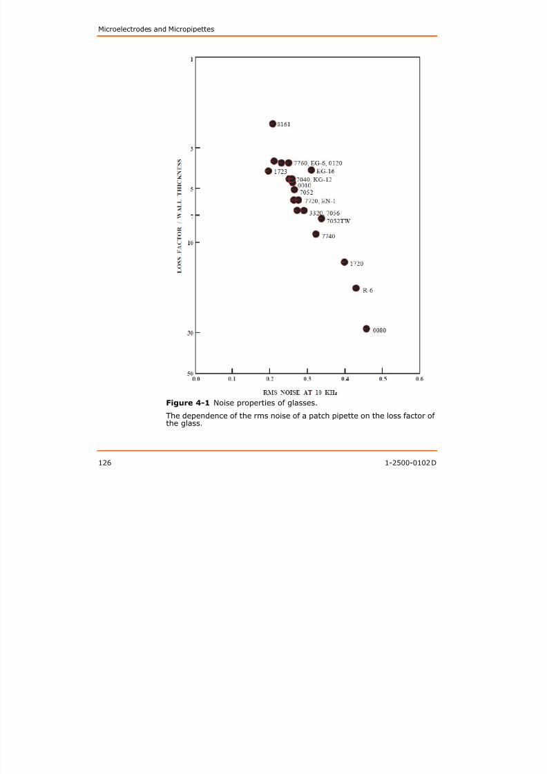
8/13/2019 User Guide v3
http://slidepdf.com/reader/full/user-guide-v3 127/302
126 1-2500-0102 D
Figure 4-1 Noise properties of glasses.
The dependence of the rms noise of a patch pipette on the loss factor ofthe glass.
The Axon Guide to Electrophysiology and Biophysics Laboratory Techniques
As seen in Figure 4-1, glasses with the lowest loss factor exhibit thelowest noise. Furthermore, noise decreases as the wall thicknessincreases (compare 7052 with 7052TW, thin walled). Even greaterimprovement in noise can be achieved using quartz (fused silica)pipettes. The noise of pipettes fabricated from Corning 7070 (low loss
electrical) or Corning 1724 (aluminosilicate) glasses could also beimproved if proper techniques of fabricating patch pipettes from theseglasses would be developed. The noise values shown in Figure 4-1 arehigher than would be obtained with the Axopatch™ 200B amplifier insingle-channel recording mode since its capacitive headstage produceslower noise than is produced by standard resistive headstages. It hasbeen observed that as the noise of the headstage electronicsdecreases, the noise of other components, such as holder and glass, isreduced as well

8/13/2019 User Guide v3
http://slidepdf.com/reader/full/user-guide-v3 128/302
1-2500-0102 D 127
reduced as well.
Leachable Components
Glasses are complicated substances made of many differentcompounds as shown in Table 4-2. While glasses have majorconstituents that lead to their classification as soda lime,aluminosilicate, borosilicate, for example, they have many tracecompounds whose location in the glass is unknown. Glasses may havecomponents on their surfaces that can leach into an aqueous
environment with which they are in contact. Leachable componentscould be particularly problematic in single-channel and whole-cellrecording due to the close proximity of the channels to the glass. Theliterature contains reports of undesirable effects of the leaching ofconstituents from the glass on membrane currents.
Further Reading
Cota, G., Armstrong, C. M. Potassium channel “inactivation” induced bysoft-glass patch pipettes. Methods in Enzymology. Plenum Press. NewYork and London, 1983.
Sakmann, B., Neher, E. Geometric parameters of pipettes andmembrane patches. Single- Channel Recording. Sakmann, B., Neher,E., Eds. pp. 37–51. Plenum Press. New York and London, 1983.
Cota, G., Armstrong, C. M. Potassium channel “inactivation” induced bysoft-glass patch pipettes. Biophys. J. 53, 107–109, 1988.
Corey, D. P., Stevens, C. F. Science and technology of patch-recordingelectrodes. Single-Channel Recording. Sakmann, B., Neher, E. Eds. pp.53–68. Plenum Press, New York and London, 1983.
Hammill, O.P., Marty, A., Neher, E., Sakmann, B., Sigworth, F.J.Improved patch-clamp techniques for high resolution current-recordingfrom cells and cell-free membrane patches. Pflugers Arch. 391,85–100, 1981.
Microelectrodes and Micropipettes
Rae, J. L., Levis, R. A. Patch-clamp recordings from the epithelium ofthe lens obtained using glasses selected for low noise and improvedsealing properties. Biophys. J. 45, 144–146, 1984.
Rae, J. L., Levis, R. A. Patch voltage clamp of lens epithelial cells:theory and practice. Molec. Physiol. 6, 115–162, 1984.
Rae, J. L., Levis, R. A., Eisenberg, R. S. Ion Channels. Narahashi, T. Ed.pp. 283–327. Plenum Press, New York and London, 1988.
Ogden, D. C., Stanfield, P. R. Microelectrode Techniques: The PlymouthWorkshop Handbook. Standen, N. B., Gray, P. T. A., Whitaker, M. J. Eds.pp. 63–81. The Company of Biologists Limited, Cambridge, 1987.
Furman, R. E., Tanaka, J. C. Patch electrode glass composition effectson ion channel currents. Biophys J. 53, 287–292, 1988.

8/13/2019 User Guide v3
http://slidepdf.com/reader/full/user-guide-v3 129/302
128 1-2500-0102 D
Rojas, L., Zuazaga, C. Influence of the patch pipette glass on singleacetylcholine channels recorded from Xenopus myocytes. Neurosci.Lett. 88: 39–44, 1988.
5Advanced Methods in Electrophysiology
Recording from Xenopus Oocytes
The Xenopus oocyte expression system was introduced by Gurdon in1971 as a means to study various aspects of the control of geneexpression. Injection of exogenous DNA into the oocyte nucleus ormRNA into the cytoplasm led to the expression of functional proteins bythe oocytes. Early studies dealt with the expression of proteins that areof little interest to electrophysiologists, such as globin, interferon andvarious viral proteins Consequently electrophysiologists and

8/13/2019 User Guide v3
http://slidepdf.com/reader/full/user-guide-v3 130/302
1-2500-0102 D 129
various viral proteins. Consequently, electrophysiologists and
biophysicists paid scant attention to studies of protein expression inoocytes. However, beginning in 1982, Miledi and co-workersdemonstrated that various types of ion channels and receptors couldalso be expressed in oocytes after injection of mRNAs that had beenisolated from the appropriate tissue. For example, injection of Torpedoelectric organ mRNA led to the expression of functional nicotinicacetylcholine receptors, while injection of rat brain mRNA resulted inthe expression of a large number of different voltage- and ligand-gatedion channels, among them the voltage-gated Na+ channels, NMDA and
non-NMDA subtypes of glutamate receptors, and GABAA receptors.Since these initial experiments, a number of workers have adopted thisexpression system to study various aspects of the structure andfunction of ion channels and receptors. Some of the more commontypes of studies that have employed expression of exogenous ionchannels and receptors in oocytes include:
1. Analyzing the properties of mutated channels as a means tounderstand structure-function relationships in ion channels;
2. Studying the post-translational processing and the assembly ofmultisubunit channels and receptors;
3. Comparing the properties of channels from various tissuesexpressed in a common environment;
4. Examining the modulation of channel and receptor function byvarious second messenger systems;
5. Analyzing various aspects of receptor-effector coupling; and
6. Functional screening of cloned genes that encode channels andreceptors (expression cloning).
Most of these experiments involve electrophysiological recording fromoocytes. This describes the mechanics of recording from oocytes andpoints out some oocyte features of which one should be aware in orderto obtain high-quality recordings.
Advanced Methods in Electrophysiology
What is a Xenopus Oocyte?
Xenopus oocytes are egg precursors that, upon proper hormonalstimulation, pass through the frog’s oviduct and become eggs, whichcan then be fertilized to make more frogs. Oocytes are stored in the
abdominal cavity and can be removed surgically for experimentalpurposes. They go through six developmental stages (termed stages Ito VI). Most researchers use only the large stage V and VI oocytes,which can be used interchangeably in electrophysiological experiments.Oocytes are found in clumps called ovarian lobes, which are made up ofoocytes, connective tissue, blood vessels and follicle cells. Figure 5-1 shows an individual stage V or VI oocyte as found in an ovarian lobe.
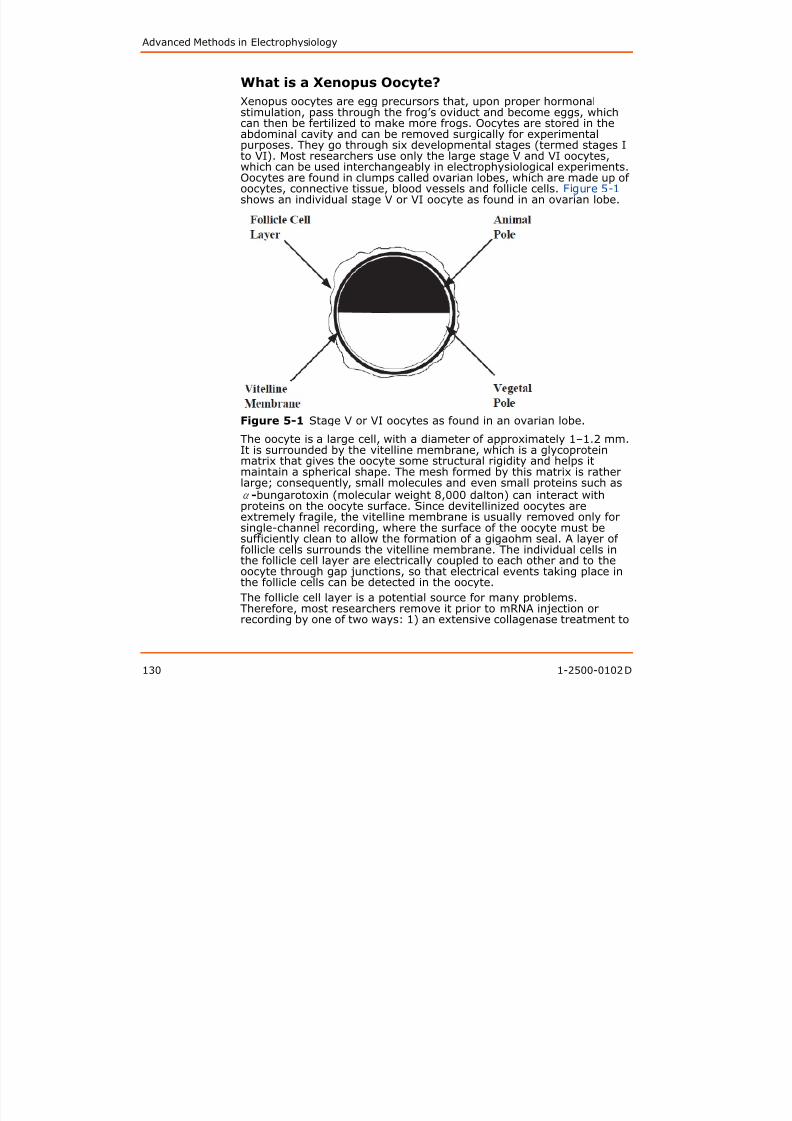
8/13/2019 User Guide v3
http://slidepdf.com/reader/full/user-guide-v3 131/302
130 1-2500-0102 D
Figure 5-1 Stage V or VI oocytes as found in an ovarian lobe.
The oocyte is a large cell, with a diameter of approximately 1–1.2 mm.It is surrounded by the vitelline membrane, which is a glycoproteinmatrix that gives the oocyte some structural rigidity and helps itmaintain a spherical shape. The mesh formed by this matrix is ratherlarge; consequently, small molecules and even small proteins such asα-bungarotoxin (molecular weight 8,000 dalton) can interact withproteins on the oocyte surface. Since devitellinized oocytes areextremely fragile, the vitelline membrane is usually removed only forsingle-channel recording, where the surface of the oocyte must besufficiently clean to allow the formation of a gigaohm seal. A layer of
follicle cells surrounds the vitelline membrane. The individual cells inthe follicle cell layer are electrically coupled to each other and to theoocyte through gap junctions, so that electrical events taking place inthe follicle cells can be detected in the oocyte.
The follicle cell layer is a potential source for many problems.Therefore, most researchers remove it prior to mRNA injection orrecording by one of two ways: 1) an extensive collagenase treatment to
The Axon Guide to Electrophysiology and Biophysics Laboratory Techniques
completely strip off the layer by immersing the oocyte for 1–3 hours ina calcium-free saline containing 2 mg/mL collagenase Type IA (SigmaChemical Company, St. Louis, MO) until about half of the oocytes havebeen released from the ovarian lobe; or 2) a less extensive collagenasetreatment followed by manual removal of the follicular layer with
watchmaker’s forceps. The latter is preferred, since oocytes thatundergo the extensive collagenase treatment sometimes do not surviveas long as those treated less extensively. Some of the problemsintroduced by the follicle cell layer are rather trivial. For instance, it ismore difficult to impale a follicle-encased oocyte with an injectionneedle or a microelectrode. Other complications, however, can createmajor problems. The electrical coupling between the oocyte proper andthe follicle cells means that one records from both. Numerous examplesof oocyte “endogenous” receptors that turned out to be in the folliclecell layer were published In fact the Xenopus oocyte is a nearly ideal
8/13/2019 User Guide v3
http://slidepdf.com/reader/full/user-guide-v3 132/302
1-2500-0102 D 131
cell layer were published. In fact, the Xenopus oocyte is a nearly idealexpression system for ion channels and receptors since it has very fewtypes of endogenous channels and receptors, an advantage that isdefeated if the follicle cells are left on the oocyte.
One of the striking features of a Xenopus oocyte is its two-toned colorscheme: the animal pole hemisphere is dark colored, while the vegetalpole is light colored. This polarity is maintained inside the oocyte: thenucleus is found in the animal pole, and different populations of mRNAsexist in the hemispheres. In addition, a standing Cl- current flows fromone pole to the other, indicating that the distribution of channels in theoocyte membrane is not homogeneous. Published reports showed thatACh receptors expressed from exogenous mRNAs are also unevenlydistributed; although receptors were expressed all over the oocyte,more receptors were expressed on the vegetal pole. It is not clear ifthere is any relation between the site of RNA injection and the locationof the expressed channels on the oocyte membrane. Thisnon-homogeneity is not important for whole-cell recording, but couldbe important for single-channel recording.
Two-Electrode Voltage Clamping of OocytesTwo factors need to be taken into consideration when voltage clampingoocytes. First, with an apparent surface area on the order of 106 μm2,there is an enormous amount of membrane that must be charged inorder to clamp the cell. In fact, the situation is even worse than it mayappear since there is considerable invagination of the surfacemembrane, thereby doubling or even tripling the surface areacompared to an “ideal” spherical oocyte. Second, one can encountercurrents up to 10 μA or larger after mRNA injection, potentially causingappreciable series resistance errors. In the case of currents from clonedK+ and Na+ channels, which activate rapidly and can give rise to verylarge currents, there may be an inadequate control of the voltageduring the initial phases of channel activation.
Advanced Methods in Electrophysiology
The response time (τ) of a voltage clamp to a step voltage change is:
where RI is the resistance of the current-passing electrode, Cm is themembrane capacitance, and A is the gain of the command amplifier.Since not much can be done about Cm (Combining Whole-Cell Clampwith Focal Current Recording on page 144), the only two things one cando in order to achieve fast clamping of the cell is to use the lowest RI and largest A possible. One “advantage” of the oocyte’s large size isthat one can use low-resistance electrodes for both thevoltage-recording and current-passing electrodes. (This can hardly beregarded as an advantage, since the large size of the oocyte is what

8/13/2019 User Guide v3
http://slidepdf.com/reader/full/user-guide-v3 133/302
132 1-2500-0102 D
caused the problem in the first place). Electrodes that have resistancesof 0.5–2 MΩ when filled with 3 M KCl are used. The particular type ofglass is unimportant; both regular and fiber-filled electrode glass havebeen used successfully. Since the electrodes have rather large tipopenings, they usually do not clog very often; the same set ofelectrodes can be used repeatedly during the course of a day. Theelectrodes’ low resistance eliminates the need in anegative-capacitance circuit to correct for the frequency response ofthe voltage-recording electrode, thereby eliminating this potentialsource of clamp instability. To achieve the fastest response, theelectrodes must be shielded in order to reduce capacitive couplingbetween them. Two rather simple ways of doing this are 1) Placing agrounded sheet of metal between the two electrodes (making sure thatit doesn’t make contact with the bath), or 2) wrapping a wire around apiece of tubing that fits over the voltage electrode like a sleeve, andthen grounding the wire. In the latter case, the shield should extend asclose to the bath as possible.
The other parameter that one can control in order to maximize thespeed of the voltage clamp is the command amplifier gain. As with
other types of cell-electrode combinations, one must usually introducea frequency response compensation network to ensure clamp stabilityat high gains. Therefore, the absolute gain of the clamp and thecommand voltage of the amplifier are less important than themaximum gain reached before the clamp becomes unstable. The LAGand (AC) GAIN controls of the Axoclamp™ 900A microelectrodeamplifier allow one to fine-tune the clamp. For oocytes, start with theLAG at about 0.2 ms and the GAIN set to its lowest position, andgradually increase it as much as possible until the clamp starts
oscillating. The lower the LAG setting, the faster the clamp. Axoclamp900-series amplifiers include an Oscillation Detection circuit thatautomatically reduces the voltage clamp gain when oscillation in thecircuit is detected.
The goal is to achieve a fast voltage clamp. But, how fast is fastenough? The actual speed required depends on the type of signal beingmeasured. For example, when studying a ligand-activated ion channel
The Axon Guide to Electrophysiology and Biophysics Laboratory Techniques
that is activated by bath application of an agonist, it makes nodifference if the clamp settles in 2 ms or 20 ms, since the exchangetime of the chamber is the limiting factor in the rate of activation. Onthe other hand, when studying voltage-gated channels, one wants thefastest clamp attainable. A well-tuned, two-microelectrode voltage
clamp can clamp an oocyte fast enough to study the gating kinetics ofmost voltage-gated channels. However, it is probably impossible toclamp an oocyte fast enough to study the activation kinetics offast-gating voltage-gated Na+ channels in which the rising phase of thecurrent can be on the order of 1 ms or shorter. It is still possible tostudy slower processes, such as inactivation or pharmacologicalproperties, even if the clamp is not fast enough to study the activationprocess. A faster clamp can be achieved either by recording fromsmaller oocytes (stage II or III) whose capacitances are approximatelyone-fifth those of the larger stage V and VI oocytes, or applying the

8/13/2019 User Guide v3
http://slidepdf.com/reader/full/user-guide-v3 134/302
1-2500-0102 D 133
one fifth those of the larger stage V and VI oocytes, or applying themore common “macropatch” technique. Either of these two approachesprovides a sufficiently fast clamp for studying the kinetics of Na+
channel activation.
Electrode penetration is most easily achieved simply by advancing theelectrode into the oocyte until it dimples the membrane and then visiblypops into the cell. Due to the large size of the oocyte, a coarse,inexpensive manipulator provides adequate control of movement.Typical resting potentials in a physiological saline solution (100 mMNaCl, 2 mM KCl, 1.8 mM CaCl2, 1 mM MgCl2, 5 mM HEPES, pH 7.6) areapproximately - 40 mV or more negative. The voltage clamp is tunedby applying a small (2 mV) square wave at the resting potential andthen gradually increasing the gain of the clamp. As the gain increases,the voltage trace “squares up” and the capacitive transient in thecurrent trace gets faster and faster. Instability in the clamp will firstappear as small oscillations in the traces; the oscillations will increaseas the gain increases. If oscillations do appear, the TIME CONSTANTcontrol should be adjusted until they disappear. This process should becontinued until one reaches the highest gain possible without any
apparent oscillations. In general, if the electrodes are shielded asdescribed above, full gain can be achieved.
Patch Clamping Xenopus Oocytes
While oocytes are obviously too large for the whole-cell mode of patchclamping, they are amenable to all three configurations ofsingle-channel recording, i.e., cell-attached, inside-out and outside-out.One of the major requirements for achieving the high-resistance sealsnecessary for single-channel recording is a clean membrane surface.With oocytes, one must remove the vitelline membrane prior to patchclamping by placing the oocyte in a hypertonic stripping solution(usually 200 mM K-aspartate, 20 mM KCl, 1 mM MgCl2, 10 mM EGTA,10 mM HEPES, pH 7.4) and allowing it to shrink. As the oocyte shrinks,the vitelline membrane detaches from the cell membrane and appearsas a transparent sphere around the oocyte. One can then manuallyremove the vitelline membrane using fine watchmaker’s forceps. Since
Advanced Methods in Electrophysiology
devitellinized oocytes will stick to glass or plastic (but not to agarose)after a few minutes of contact, the shrinking and vitelline membraneremoval is usually carried out in small petri dishes with a layer of 2%agarose on the bottom. This allows one to prepare a number of oocytesat once. At this point, the oocytes are extremely fragile. In particular,
stripped oocytes have a propensity for disintegrating when they are atan air-water interface; therefore, extreme care must be taken whentransferring them to the recording chamber.
Once the vitelline membrane has been removed, gigaohm seals can beobtained with high success rates. Oocytes, like most cells, containstretch-activated channels that can interfere with recording “interesting” channels in the cell-attached mode. Therefore, mostresearchers prefer to use excised patches for single-channel work,where the incidence of stretch-activated channel currents is much

8/13/2019 User Guide v3
http://slidepdf.com/reader/full/user-guide-v3 135/302
134 1-2500-0102 D
lower. The actual mechanics of obtaining excised patches is the sameas for any cell type, with the exception that some researchers prefer torupture the membrane by applying positive pressure rather thansuction, since suction can sometimes cause yolk platelets to clog thepipette tip.
Further Reading
Barnard, E.A., Miledi, R., Sumikawa, K. Translation of exogenous
messenger RNA coding for nicotinic acetylcholine receptors inducesfunctional receptor in Xenopus oocytes. Proc. R. Soc. Lond. B215:241–246, 1982.
Gurdon, J.B., Lane, C.D., Woodland, H.R., Marbaix, G. Use of frog eggsand oocytes for the study of messenger RNA and its translation in livingcells. Nature. 233:177–182, 1971.
Krafte D., Lester, H.A. Expression of functional sodium channels instage II–III Xenopus oocytes. J. Neurosci. Meth. 26:211–215, 1989.
Methfessel, C., Witzemann, V., Takahashi, T., Mishina, M., Numa, S.,Sakmann, B. Patch clamp measurements on Xenopus laevis oocytes:currents through endogenous channels and implanted acetylcholinereceptor and sodium channels. Pflugers Arch. 407:577–588, 1986.
Snutch, T.P. The use of Xenopus oocytes to probe synapticcommunication. Trend Neurosci. 11:250–256, 1988.
Stuhmer, W., Methfessel, C., Sakmann, B., Noda, M. Y., Numa, S. Patchclamp characterization of sodium channels expressed from rat braincDNA. Eur. Biophys. J. 14:131–138, 1987.
Stuhmer, W., and Parekh, A.B., Electrophysiological Recordings fromXenopus Oocytes in Single-Channel Recording, 2nd Ed., Sakmann, B.,and Neher, E., eds., pp. 341–355, 1995.
The Axon Guide to Electrophysiology and Biophysics Laboratory Techniques
Patch-Clamp Recording in Brain Slices
Although it is commonly accepted that patch-clamp techniques offermany technical advantages over conventional intracellularmicroelectrode recording configurations, one nagging limitation has
been the belief that, in order to allow formation of gigaohm seals withpatch electrodes, cells must be treated in some way that leaves theirmembrane “clean.” Such treatment might entail dissociation of tissueby enzymatic digestion or mechanical disruption, and might or mightnot be followed by growth in tissue culture. These techniques invariablyresult in significant damage to the cells or severe alteration of theirenvironment, at least transiently, during the preparation of the cells forrecording. Alternatively, tissue explants or slices can be maintained in “organotypic” culture, allowing many of the cell-cell interactions to be

8/13/2019 User Guide v3
http://slidepdf.com/reader/full/user-guide-v3 136/302
1-2500-0102 D 135
maintained and mitigating some of the problemsdescribed above. However, with any of these approaches, the possibilityremains that significant alteration of cellular properties occurs prior torecording.
Therefore, it is of great interest to be able to apply patch-recordingtechniques to neurons in acute tissue slices. The marriage of these twoapproaches offers many of the advantages of both, with few of thelimitations:
1. Cells in tissue slices are likely to be much closer to their originalstate than cells subjected to the above-mentioned treatments.No disruption of the normal cellular environment need takeplace until the preparation of slices and disruption is limited tothe surface of the slice.
2. The increased signal-to-noise ratio and improved voltage-clampquality, compared with conventional intracellular recording usingsharp microelectrodes, provide substantial benefits for cellularelectrophysiology. These benefits are particularly helpful whenmeasuring small or rapid events.
3. The ability to control the intracellular environment is greatlyenhanced by whole-cell recording, thus facilitating the study ofinteractions between intracellular biochemistry andelectrophysiology.
It should be noted however, that not all problems are solved byapplying whole-cell techniques. “Washout” of intracellular biochemicalmachinery may affect electrophysiological properties, and control ofmembrane potential in branched or elongated neurons is often
inadequate.Two strategies have been applied in obtaining patch-clamp recordingsfrom tissue slices. One approach, the “cleaning” technique, involvesremoving overlying neuropil or cellular debris from a visually-identifiedcell using a relatively large pipette filled with the same solution used tosuperfuse the slice. Recording is then possible in a manner similar tostandard patch recording. In the other approach, called the “blind”
Advanced Methods in Electrophysiology
technique, the recording pipette is lowered into a tissue slice withouthigh-magnification visual guidance; seal formation is monitored usingelectrical measurements.
The Cleaning Technique
Tissue preparation for this technique uses procedures slightly modifiedfrom those used for standard slices. The slices must be thin enough toallow good cellular visibility (100–300 μm, depending on the age of theanimal), but thicker slices result in a greater number of undamagedcells. Generally, vibrating microtomes are preferable to tissue choppersbecause their use results in less dead or damaged tissue at the cutsurface, and because they facilitate preparation of thin slices. Specialcare should be taken when preparing thin slices to ensure that thebathing medium remains ice cold in order to maintain the necessaryfi i i F ll i h i i d i

8/13/2019 User Guide v3
http://slidepdf.com/reader/full/user-guide-v3 137/302
136 1-2500-0102 D
firm tissue consistency. Following their preparation and prior torecording, slices are commonly incubated at 37°C for about one hour.This procedure softens the tissue and facilitates subsequent cleaning ofcells. Various methods may be used for storing slices, but care isneeded to avoid damage to the cut surfaces resulting from proceduressuch as placing slices on filter paper. Slices may be stored at roomtemperature or warmed to 30–35°C.
The only major piece of equipment required for this technique, inaddition to a standard recording setup, is an upright microscope
equipped with a water-immersion objective, most commonly 40xmagnification. Use of an inverted microscope is not feasible since, evenif very thin slices are used, visibility through the tissue to a recordingpipette is significantly impaired. Hoffman or Nomarskidifferential-interference-contrast optics can be helpful, but are notnecessary. Unless manipulators are mounted on the stage, it isextremely helpful to use a fixed-stage microscope, so that changingfocus does not cause movement of the tissue with respect to cleaningor recording pipettes.
An objective with high numerical aperture is important. A commonlyused apparatus is the Zeiss 40x water-immersion objective, which hasa numerical aperture of 0.75. This objective offers a working distanceof approximately 1.6 mm. The pipettes must, therefore, be placed at avery shallow angle (15° from the horizontal is common). Oneconsideration in mounting micromanipulators is that the movement intrue horizontal and vertical directions is preferable to a coordinatesystem with an axis oriented parallel to the pipette. An advantage ofthis arrangement is the ability to lower the recording pipette directly
onto the target cell in a single motion.The recording chamber must allow continuous superfusion of the slice;it must also permit immobilization of the tissue despite the fluid flow,and do so using a device that does not interfere with the objective orthe pipettes. One solution to this problem is a net consisting of aU-shaped piece of flattened platinum wire with a parallel array of veryfine nylon monofilaments, such as stocking fibers, glued across the
The Axon Guide to Electrophysiology and Biophysics Laboratory Techniques
arms of the U-shaped wire (Edwards et al., 1989; Sakmann et al.,1989). The net can be placed on the slice and is usually heavy enoughto prevent movement. Although the filaments may cause some damageto the surface of the tissue, they may be placed sufficiently far apart toleave considerable working space (the precise distance depends on the
cellular architecture in the slice). Another solution is to attach the sliceto the bottom of the recording chamber using a plasma clot (Blanton etal., 1989).
The pipette used for cleaning should have a tip much larger in diameterthan a recording pipette, usually in the range of 5–20 μm. The optimaltip size depends on several factors; in general, larger tips arepreferable for larger cells and for deeper cleaning. However, theconsistency of the tissue and cell density may also affect the choice oftip diameter. For example, with particularly “sticky” tissue, such as
t ll l i i tt t d t b l d ith

8/13/2019 User Guide v3
http://slidepdf.com/reader/full/user-guide-v3 138/302
1-2500-0102 D 137
neocortex, small cleaning pipettes may tend to become clogged withmembranous debris. For a given preparation, it is best to arriveempirically at an appropriate size. Additionally, since debris tends toaccumulate on the jagged edges of broken pipettes, it is usually best topull unbroken pipettes to the appropriate size. To minimize any damagethat the process might inflict on the cell, the cleaning pipette should befilled with the same solution used for the bathing medium. Note thatsome researchers, instead of using a separate cleaning electrode,perform the cleaning with the same recording electrode for the sake ofexpediency.
The first step in establishing a recording is to locate a healthy cell. It isusually possible to distinguish cells in good condition by theirappearance of solidity or opacity. In such neurons, it is often possible tofollow dendritic processes for some distance. Some healthy cells maybe observed whose somata are on the surface of the slice and whichdisplay a “clean” membrane suitable for immediate patching with nofurther cleaning. Such neurons often have dendrites that can be seenprojecting into the depths of the slice. It seems that cells that have lostmost of their dendrites due to the slicing procedure are often “sick,” as
characterized by a granular and/or transparent appearance of thesoma.
Once a healthy cell has been located, the next step is to remove theoverlying neuropil. Mouth control of the pressure applied to the back ofthe pipette permits rapid, highly precise application of pressure andsuction. It is often best to begin by applying positive pressure gentlywith the pipette placed just at the surface of the slice and directlyabove the targeted cell. Blowing accomplishes two goals. First, itprovides information about the consistency of the tissue, which may be
rather variable from slice to slice and which differs dramatically fromone brain region to another. Second, application of positive pressurebegins the process of disrupting the tissue overlying the desired cell.When tissue has been visibly disrupted, slight suction helps remove theloosened debris (Figure 5-2). Repeated application of this blowing andsucking cycle, with appropriate movement of the pipette to removespecific chunks of tissue, eventually results in a clean cell.
Advanced Methods in Electrophysiology

8/13/2019 User Guide v3
http://slidepdf.com/reader/full/user-guide-v3 139/302
138 1-2500-0102 D
Figure 5-2 The Cleaning technique. Use of a cleaning pipette toremove tissue overlying a cell in tissue slices. Reproduced withpermission according to Edwards et al., (1989).
The Axon Guide to Electrophysiology and Biophysics Laboratory Techniques
At first, this procedure may take a long time. It is almost inevitable thatan inexperienced experimenter, who has not yet developed a feel forthe tissue, will kill cells by applying pressure or suction that is toovigorous. With practice, however, one can clean even deep cells quiterapidly. Careful and repeated adjustment of the focus aids greatly in
determining the degree of cleaning required at each stage. Dependingon the particular type of tissue, a few tricks to facilitate and acceleratethe process of producing clean cells may be applied. For example, inregions of densely packed somata, such as the CA1 pyramidal cell layerof the hippocampus, it is possible to remove tissue at the slice surfaceover a relatively large length of the cell layer by applying continuoussuction and moving the pipette along the layer as if using a vacuumcleaner to remove dead tissue. Inspection of the underlying neuronsoften reveals at least one clean pyramidal cell.
After completing the cleaning procedure patch-clamp recordings ofcleaned cells in slices are carried out following essentially the same
8/13/2019 User Guide v3
http://slidepdf.com/reader/full/user-guide-v3 140/302
1-2500-0102 D 139
After completing the cleaning procedure, patch-clamp recordings ofcleaned cells in slices are carried out following essentially the sameprocedures that would be applied to cells in culture. All four majorpatch-recording configurations (cell-attached, inside-out, outside-outand whole-cell) are possible, as well as the nystatin-perforated patchtechnique (see Recording from Perforated Patches and PerforatedVesicles on page 154).
The Blind Technique
Apart from a microelectrode holder with the appropriate diameter forpatch pipettes, and with a side port for pressure application, no specialequipment is necessary to adapt a standard slice setup equipped forintracellular recording to one suitable for blind-patch recording. Adissecting microscope is sufficient. The recording pipette should have aresistance in the bath of approximately 3–5 MΩ; the optimal resistancedepends on the size and type of cell being recorded.
The procedure for establishing gigaohm seals is very simple (Figure 5-3). It is possible to use either the current-clamp or voltage-clamp
recording mode. A small repetitive current or voltage pulse is applied tothe electrode at relatively high frequency (for example, 10 Hz) and thevoltage or current response is monitored with an oscilloscope.Continuous, slight pressure is applied to the back of the pipette, forexample, by blowing gently into the tubing connected to the pipetteand closing a stopcock to retain the pressure. The pipette is then slowlylowered into the tissue in the region where the desired cells are found.It is advanced slowly (1–5 steps per second, each step of 1–2 μm) intothe tissue until a sudden increase in resistance is detected at the
pipette tip, indicating contact with a cell. Often a further advance of1–2 μm causes a further increase in the resistance. Release of thepositive pressure should result in another approximate doubling of theresistance if the electrode is indeed contacting a cell. Although gigaohmseals sometimes form spontaneously at this stage, the next step is toapply light suction to cause the seal to form. This may occur rapidly, inless than one second, or slowly, up to several seconds, requiring
Advanced Methods in Electrophysiology
constant, gentle suction. The patch is then ruptured by additionalsuction creating electrical continuity between the pipette and cellinterior.
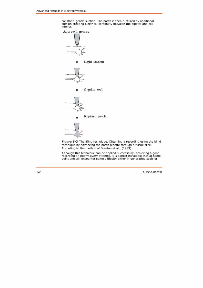
8/13/2019 User Guide v3
http://slidepdf.com/reader/full/user-guide-v3 141/302
140 1-2500-0102 D
Figure 5-3 The Blind technique. Obtaining a recording using the blindtechnique by advancing the patch pipette through a tissue slice.According to the method of Blanton et al., (1989).
Although this technique can be applied successfully, achieving a goodrecording on nearly every attempt, it is almost inevitable that at somepoint one will encounter some difficulty either in generating seals or
The Axon Guide to Electrophysiology and Biophysics Laboratory Techniques
establishing whole-cell recordings. Through experience, it is possible toidentify the problem-causing aspects of the procedure. Often, changingthe pipette size helps. A general rule is to use smaller tips to improvesealing, and larger ones to facilitate the transition to the whole-cellmode. One should be prepared to use a number of pipettes, since the
probability of obtaining a recording on the second attempt to applysuction to the same pipette is very small. Another critical variable,which applies to all patch-clamp recording, is the intracellular solutionwhose osmolarity should be verified routinely, particularly whendifficulties are encountered.
Advantages and Disadvantages of the two Methods ofPatch Clamping Brain Slices
It is impossible to give a complete discussion of the relative merits ofthe cleaning and blind techniques here. However, some of the

8/13/2019 User Guide v3
http://slidepdf.com/reader/full/user-guide-v3 142/302
1-2500-0102 D 141
t s poss b e to g e a co p ete d scuss o o t e e at e e ts othe cleaning and blind techniques here. However, some of theimportant considerations are outlined in the following table.
Table 5-1 Brain Slice Techniques.
Cleaning Technique Blind Technique
Need upright microscope and waterimmersion objective.
Need no special equipment beyond thatfor intracellular recording in slices.
Vibrating microtome almostessential. Vibrating microtome stronglyrecommended, essential for sometissues.
Maximum slice thickness limited byvisibility.
Maximum slice thickness limited byviability.
Once a cell is located, additionaltime is invested in cleaning.
Less preparation time for eachpenetration, but no certainty of cellhealth.
Cell is visually identified Need post-hoc identification of celltype unless electrophysiologicalidentification is possible or ahomogeneous cell population isused.
Can see neighboring cells andapply local stimuli.
Visually-guided local stimulation isnot possible.
All four standard patch-clampconfigurations possible, plus the
perforated patch technique.
All four standard patch-clampconfigurations possible, plus the
perforated patch techniqueRecording quality similar tostandard patch clamptechniques.
High or unstable access resistance isoften a problem with whole-cellmode (possibly due to debris in thepipette tip).

8/13/2019 User Guide v3
http://slidepdf.com/reader/full/user-guide-v3 143/302
The Axon Guide to Electrophysiology and Biophysics Laboratory Techniques
employing large-diameter patch pipettes (5–10 μm tip diameter) and isused to sample currents from much larger areas than are commonlyused in single-channel recording (which is done with 0.5–2 μm tipdiameter pipettes). The second method of macropatch recording hasbeen termed loose-patch recording. This method, which enables one to
gather data that could not be obtained with the gigaseal method,differs from single-channel recording in three ways:
1. The tip of the loose-patch pipette is usually much larger thanthe conventional single-channel patch pipette;
2. The loose-patch pipette does not form a gigaseal with themembrane, whereas gigaohm seals are required forsingle-channel recording; and
3. The loose-patch pipette can be reused and repositioned to mapthe spatial distribution of channel subtypes on individual cells(Thompson and Coombs, 1988).

8/13/2019 User Guide v3
http://slidepdf.com/reader/full/user-guide-v3 144/302
1-2500-0102 D 143
Gigaseal-Macropatch Voltage Clamp
Macroscopic patch currents can be recorded using standardpatch-clamp instrumentation and a large patch pipette having aresistance of a few hundred kilohms. A gigaseal is formed usingsuction. This method can be applied to cell-attached and excisedpatches. Data analysis uses the same methods that are applied in
whole-cell clamp experiments. Consequently, data concerning thekinetic behavior and local amplitude of ionic currents can be rapidlyacquired. This method has been used to record macroscopic currents inXenopus oocytes (Hoshi et al., 1990), which are particularly amenableto this method of recording because channel expression can becontrolled, to a certain degree, by the experimental conditions.
There are a few problems associated with this method that have to beconsidered in the experimental design. The patch-clamp amplifier mustbe able to fully compensate for the greater capacitance of larger
patches. When voltage pulses are applied to macropatches in thecell-attached configuration, current flowing in the patch will change thecell voltage; this change can be significant. For example, with amacropatch current of 100 pA and a cell input resistance of 100 MΩ,the cell voltage will change by 10 mV. Dynamic currentdependenterrors of this type are difficult to correct and are most severe in smallcells. In some preparations it may be impossible to use cell-attachedmacropatches to obtain accurate I/V curves, especially for rapidlychanging currents. One can eliminate this source of error by studyingexcised patches.
Milton & Caldwell (1990) identified a more subtle error associated withmacropatch recording. They observed that the suction used to form theseal between the patch pipette and the membrane can cause a changein ion channel density in the patch. With large patch pipettes, anoticeable membrane bleb may form in the orifice of the pipette duringsuction. This membrane bleb can be visualized under a microscope. It
Advanced Methods in Electrophysiology
appears that the ion-channel density decreases during bleb formation,possibly because of a flow of lipid into the bleb causing membranerearrangement and changes in channel distribution. Therefore, thegigaseal-macropatch method may be unsuitable for mappingion-channel densities because the procedure modifies the channel
density before the measurement is made.
Loose-Patch Voltage Clamp
In loose-patch recording it is not necessary to form a tight sealbetween the patch pipette and the plasma membrane. Therefore,strong suction is not needed. This has at least two advantages:
1. The pipette can be repositioned to sample currents from anumber of patches on the same cell; and
2. The loose-patch method can be used to measure local currentsin voltage-clamped preparations where establishing gigaseals is

8/13/2019 User Guide v3
http://slidepdf.com/reader/full/user-guide-v3 145/302
144 1-2500-0102 D
g p p p g g gimpossible due to the presence of adherent connective tissue,basement membrane or glial cells. Note that loose-patchrecording is done only in the cell-attached configuration.
The low seal resistance between the pipette and the membranepresents the principal technical difficulty one must overcome inapplying loose-patch methods. Low seal resistance creates two types ofproblems. First, the current flowing through the seal resistance and
capacitance introduces noise in the current record, thus limiting theresolution (see The Importance of a Good Seal on page 99). A moresignificant problem arises from the fact that membrane current flowingthrough the seal resistance is lost.
The following discussion will focus on the errors introduced by low sealresistance and the procedures used to limit errors to acceptable levels.Three designs are available to combat the problems associated with lowseal resistance in loose-patch recording. The choice of the mostappropriate method depends on the nature of the preparation. The
original literature should be consulted for further details.Combining Whole-Cell Clamp with Focal Current Recording
The first method to be introduced combines whole-cell voltageclamping with loose-patch current recording. This is the preferredmethod for many applications. The cell is voltage clamped by amicroelectrode or a whole-cell patch pipette using standardmicroelectrode voltage-clamp or patch-clamp instrumentation, whilecurrent is recorded from a restricted area of membrane with a
loose-patch pipette using patch-clamp instrumentation. Voltage-clamppulses are applied via the whole-cell clamp while the loose-patchpipette is maintained at the bath potential to ensure that no currentflows across the seal resistance. This method has been used to recordlocal currents in large molluscan neurons (Neher and Lux, 1969;Johnson and Thompson, 1989; Thompson and Coombs 1989; Premacket al., 1990) and in muscle cells (Almers et al., 1983). The method is
The Axon Guide to Electrophysiology and Biophysics Laboratory Techniques
particularly well suited for measuring the kinetics and current/voltagerelationships of macroscopic currents expressed in Xenopus oocyteswhere a whole-cell voltage clamp is severely limited by the largecapacitance of the cell and high intracellular series resistance. Theelectrode arrangement is shown in Figure 5-4.

8/13/2019 User Guide v3
http://slidepdf.com/reader/full/user-guide-v3 146/302
1-2500-0102 D 145
Figure 5-4 Combining whole-cell voltage clamping with loose-patchcurrent recording.
Schematic diagram of a cell with voltage clamp electrodes and the large
patch pipette in place. The symbols used in the figure are as follows: A,voltage clamp open loop gain; Cc, coupling capacitance betweenvoltage clamp current electrode and patch electrode; Cmp, capacitanceof membrane patch; Ic, current error; Im, membrane current suppliedby voltage clamp; Ip, patch membrane current supplied by patch clampamplifier; Rei, resistance of voltage clamp current electrode; Rp, axialresistance of patch electrode; Rsl, resistance of seal between patchpipette and cell membrane; Rsr, series resistance between the outsideof the patch electrode and the bath clamp amplifier; Vc, voltage clamp
command voltage; Vo, voltage clamp output voltage. Reproduced withpermission according to Johnson and Thompson (1989).
A reusable loose-patch pipette (5–20 μm in diameter; axial resistance(Rp) of 100–500 kΩ) is used in cell-attached configuration. Theresistance of the seal is monitored by applying test voltage steps viathe patch amplifier and measuring the amplitude of the resulting
Advanced Methods in Electrophysiology
current steps. After contacting the cell, gentle suction is applied untilthe sum of the seal resistance (Rsl) and the axial resistance of thepipette (Rp) increases by at least 10 fold; increases greater than100-fold are common. The suction is released to avoid pulling a “finger”of membrane and cytoplasm into the pipette since this would increase
the series resistance and lead to errors in voltage control and currentmeasurement. Since the lumen of the loose-patch pipette is held at thebath potential and Rp is low compared to Rsl, there is no need tocompensate for the finite value of Rsl.
This method allows one to simultaneously measure whole-cell andpatch currents as well as whole-cell and patch capacitances. The areasof the cell and of the patch can be estimated by measuring thewhole-cell and patch capacitances. A convenient way to do this is toapply a triangle-wave voltage command to the whole-cell voltage clamp
and record the resulting whole-cell and patch current waveforms. Thepatch capacitance (c) is calculated from the change in the timederivative of the voltage (dV/dt) at a vertex of the triangle wave and

8/13/2019 User Guide v3
http://slidepdf.com/reader/full/user-guide-v3 147/302
146 1-2500-0102 D
derivative of the voltage (dV/dt) at a vertex of the triangle wave andthe corresponding jump in patch current (I), using the followingequation (Neher, 1971; Palti, 1971):
Because the voltage of the patch pipette is equal to the bath voltageand only the voltage across the membrane patch covered by thepipette is changing, the capacitance of the patch pipette itself isrejected. The capacitance of the whole cell is measured in a similarfashion. However, the interpretation is complicated by currentcontributed from poorly clamped regions (see Johnson and Thompson(1989) for further discussion).
There are several issues to consider when applying this combinedvoltage-clamp method. The most important requirement is that the
patch current must be measured from a well-clamped region ofmembrane, for example, from a region that is “space clamped” by thewhole-cell voltage clamp amplifier. In order to accurately measurecurrent-voltage relationships and limit the capacitive current flowingacross the patch during voltage steps, the loose-patch pipette shouldbe positioned close to the point where the whole-cell voltage iscontrolled. Cell geometry and electrode positioning should beconsidered when designing the physical layout of the experiment.These considerations limit the kinds of preparations that can be studiedwith the method. It is reasonable to use the loose-patch pipette to
record local current densities at different points on a well-clampedspherical cell body. However, it would be inappropriate to record patchcurrents from a thin dendrite when the voltage clamp is applied to thesoma.
The most significant error results from current flowing in the sealresistance between the loose-patch pipette and the bath. This error
The Axon Guide to Electrophysiology and Biophysics Laboratory Techniques
current (Ie), which is not measured by the patch-clamp amplifier, isgiven by:
where Rp is the resistance of the loose-patch pipette and Rsl is the sealresistance. If (Rp + Rsl) is ten times larger than Rp the error in themeasured current is 10%. To minimize the error, one can reduce Rp byusing a patch pipette with a blunt taper and increase Rsl by usingsuction to improve the seal with the membrane. Enzyme treatmentwith dispase, pronase or trypsin can be used to clean the cell surfaceand improve the seal resistance.
Two kinds of errors caused by series resistance should be considered:1. The voltage drop that results from macroscopic patch currentsfl i th h th i l i t f th t h i tt (R ) ill
8/13/2019 User Guide v3
http://slidepdf.com/reader/full/user-guide-v3 148/302
1-2500-0102 D 147
flowing through the axial resistance of the patch pipette (Rp) willproduce an insignificant error in most cases. For example, if thevalue of Rp is 300 kΩ and the maximal patch current is 500 pA,the resulting voltage error is 0.15 mV.
2. A more troublesome error occurs when the bath voltage outsidethe patch pipette changes due to large whole-cell currentsflowing in the series resistance (Rsr) between the cell membrane
and the bath ground or virtual ground.The error current is given by:
where Rsr is the sum of the series resistances of the bath, the agarbridges and the liquidsilver chloride junction at the bath electrode; ittypically has a value of several kilohms.
Bath series resistance creates an insidious problem when membranecurrents are large. However, the error can be reduced by measuring thebath voltage with a separate electrode and using it as the referencevoltage at the patch-clamp amplifier. Good practice dictates that thebath voltage be used to correct the membrane voltage signal applied tothe whole-cell clamp amplifier as well. Instability can result, however, ifthe bath voltage is measured with a greater bandwidth than themembrane voltage. To remedy this, one can limit the frequencyresponse of the bath voltage follower, but this degrades performance
and causes other errors. A better solution is to eliminate the need tosubtract the bath voltage at the other circuits by voltage clamping thebath to ground potential. This can be accomplished using anindependent voltage-clamp amplifier operating at a high gain andbandwidth. Two separate agar bridges and silver-chloride electrodescan be used to measure the bath voltage and pass current to the bath.
Advanced Methods in Electrophysiology
Because of the low resistance of these electrodes, a simple voltage-clamp circuit employing a single operational amplifier is adequate forclamping the bath to ground potential. This arrangement ensures thatthe bath voltage does not change during clamp steps. The output of thecircuit provides the record of whole-cell current.
Other problems can be overcome by a careful design of theexperimental layout. Since this method uses several voltage-clampamplifiers working simultaneously, it is necessary to limit capacitivecoupling between electrodes. This can be achieved by inserting agrounded shield between the whole-cell current electrode and themacropatch pipette, and by lowering the volume of saline to theminimum required for covering the cell. To reduce high frequency noisein the patch recording, the submerged tip of the pipette should becoated with Sylgard (Dow Corning, Midland, MI) and only the tip shouldbe filled with saline. Johnson and Thompson (1989) provide a thoroughanalysis of the problems and the approaches used to reduce errors toacceptable levels.
8/13/2019 User Guide v3
http://slidepdf.com/reader/full/user-guide-v3 149/302
148 1-2500-0102 D
acceptable levels.
Voltage Pulses Applied to the Loose-Patch Pipette
Ionic currents can also be studied by applying voltage pulses directly tothe loose-patch pipette, thus eliminating the need for an independentwhole-cell clamp. Errors resulting from the finite seal resistance andthe axial resistance of the pipette are more severe in this case and
require more elaborate compensation. The advantage of this method isthat membrane currents can be recorded locally without the need toestablish an overall space clamp. This loose-patch method has beenvery successful in studies of acetylcholine (ACh) receptor andNa+-channel distribution near muscle end-plates (Almers et al.,1983a,b).
Although extra effort is required with this method, it may be the bestapproach for some preparations. It is important to remember thatcurrent flowing across a macropatch can cause a significant change in
cell voltage. In its simplest form, this method uses a large diameterpatch pipette in a cell-attached configuration and a conventionalpatch-clamp amplifier (Almers et al., 1983a,b; Stuhmer et al., 1983).In this configuration, the axial resistance of the pipette (Rp) and theseal resistance (Rsl) act as a voltage divider. When a voltage commandpulse is applied to the pipette (Vp), it will be attenuated at the pipettetip. The voltage at the pipette tip (Vt) is given by (Stuhmer et al.,1983):
When Rsl is large, as is the case in gigaseal recordings, the error isinsignificant. In loosepatch applications, however, Rp and Rsl areapproximately equal and a large fraction of the current delivered to thepipette will flow through the seal resistance. It is necessary to correct
The Axon Guide to Electrophysiology and Biophysics Laboratory Techniques
the amplitude of command-voltage steps by a factor equal toRsl /(Rp+Rsl). To do so, Rp is measured before the pipette contacts thecell and Rp + Rsl is monitored continually throughout the experiment.Almers et al., (1983a,b) used a computer to calculate a correctionfactor A = Rsl /(Rp+Rsl) before each voltage step. The correction factor
was used to scale command-voltage steps applied by the computer by1/A to ensure that the intended voltage appeared at the pipette tip.Recorded currents were divided by A to correct for current (oftentermed leakage current) flowing through the seal resistance. Thisdigital approach to seal resistance compensation is technically sound.To implement it, the user has to develop a software program forcontinuously updating the parameters needed for scaling the amplitudeof the command pulses and correct for leakage current; an extra effortthat is well justified in some applications.
Seal resistance compensation can also be achieved with an analogcircuit. Stuhmer et al., (1983) pioneered a method that uses an activevoltage divider and potentiometers to compensate for measured values
8/13/2019 User Guide v3
http://slidepdf.com/reader/full/user-guide-v3 150/302
1-2500-0102 D 149
g p pof Rp and Rsl. Their circuit allows one to null Rp and limit the seriesresistance errors to acceptable values. When correctly adjusted, theirdesign ensures that the input impedance of the patch pipette is nearzero so that there is minimal loss of membrane current across the seal.A disadvantage of this method is that it requires the user to build aspecialized patch-clamp headstage and other circuitry following theexample provided by Stuhmer et al., (1983).
With both digital and analog seal-resistance compensation, accuracydepends on one’s ability to measure Rp and (Rsl + Rp) and on theassumption that these resistances remain constant during voltagesteps that activate conductances in the patch. The error increases asthe amplitude of the voltage step and the conductance of themembrane patch increase. It is not certain that Rp and Rsl areindependent of the current amplitude. In practice, one often observesan unexpected flattening of the current-voltage relationship for inwardor outward current activation when the voltage step or the patch
current become large. Because most of the uncertainty in currentmeasurement depends on Rsl, one should use suction and/or enzymetreatment to maximize the seal. It also helps to limit the diameter ofthe patch pipette to about 20 μm or less. Rp is minimized by usingpipettes with a blunt taper.
Loose-Patch Clamp with Concentric Patch Pipettes
Almers et al., (1984) introduced a modification of the loose-patchmethod that employs a two-chambered concentric patch electrode. The
electrode is fashioned from two glass capillaries, one inside the other,with the inner capillary held in place by support rods during the pull.The concentric electrode is pushed against the cell surface where itseparates a central membrane patch from an annular surround. Thevoltage-clamp amplifier is designed to clamp both the center patch andthe surround to the command potential. Membrane current is measuredin the central barrel of the electrode while the outer annulus acts as a
Advanced Methods in Electrophysiology
guard. Since the inner and outer barrels are at the same potentialduring the command steps, current loss from the central membraneregion to ground is minimized and Rsl takes a value that is effectivelyinfinite. This approach is historically related to vaseline-gap andsucrose-gap voltage-clamp methods. It has been used successfully to
voltage clamp mammalian skeletal muscle. However, theimplementation is somewhat difficult since it requires the constructionof an elaborate concentric electrode and some specializedinstrumentation. It may still be the best approach in some cases andthe original literature should be consulted for further details.
References
Almers, W., Stanfield, P.R., Stuhmer, W., Lateral distribution of sodiumand potassium channels in frog skeletal muscle: measurements with a
patch-clamp technique. J.Physiol. 336, 261–284, 1983a.Almers, W., Stanfield, P.R., Stuhmer, W., Slow changes in currentsthrough sodium channels in frog muscle membrane J Physiol 339

8/13/2019 User Guide v3
http://slidepdf.com/reader/full/user-guide-v3 151/302
150 1-2500-0102 D
through sodium channels in frog muscle membrane. J. Physiol. 339,253–271, 1983b.
Almers, W., Roberts, W.M., Ruff, R.L., Voltage clamp of rat and humanskeletal muscle: measurements with an improved loose-patchtechnique. J.Physiol. 347, 751–768, 1984.
Hoshi, T., Zagotta, W.N., Aldrich R.W., Biophysical and molecularmechanisms of Shaker potassium channel inactivation. Science 250,533–538, 1990.
Johnson, J.W, Thompson, S., Measurement of non-uniform currentdensity and current kinetics in Aplysia neurons using a large patchmethod. Biophys. J. 55, 299–308, 1989.
Milton, R.L., Caldwell, J.H., Na current in membrane blebs: Implicationsfor channel mobility and patch clamp recording. J. Neurosci. 10,885–893, 1990.
Neher, E., Two fast transient current components during voltage clamp
on snail neurons. J.Gen.Physiol. 58, 36–53, 1971.Neher, E., Lux, H.D., Properties of somatic membrane patches of snailneurons under voltage clamp. Pflugers Arch. 322, 35–38, 1971.
Palti, Y., Varying potential control voltage clamp on axons. in Biophysicsand Physiology of Excitable Membranes. W.F. Adelman, Jr., Ed. VonNostrand Reinhold Co. pp. 194–205, 1971.
Premack, B.A., Thompson, S., Coombs-Hahn, J., Clustered distributionand variability in kinetics of transient K channels in molluscan neuron
cell bodies. J. Neurosci. 9, 4089–4099, 1990.Stuhmer, W., Roberts, W.M., Almers, W., The loose patch clamp. inSingle-Channel Recording. Sakmann, B., Neher, E., Eds. pp. 123–132,1983.
The Axon Guide to Electrophysiology and Biophysics Laboratory Techniques
Thompson, S. and Coombs, J., Spatial distribution of Ca currents inmolluscan neuron cell bodies and regional differences in the strength ofinactivation. J. Neurosci. 8, 1929–1939, 1988.
The Giant Excised Membrane Patch MethodMany physiologically important ion pumps, exchangers andco-transporters are electrogenic. The giant excised membrane patchmethod has been developed to improve electrophysiological studies ofsuch mechanisms. Although whole-cell recording techniques are oftenemployed in transport studies, a method offering free access to thecytoplasmic membrane surface and faster voltage clamping wasstrongly desirable. While the excised membrane patch method was anattractive alternative, the conventional patch clamp techniques were
not useful. First, the single turnover rates of transporters (1–10,000per second) are far too small to expect resolution of the currentgenerated by a single transporter. Second, the magnitudes of

8/13/2019 User Guide v3
http://slidepdf.com/reader/full/user-guide-v3 152/302
1-2500-0102 D 151
generated by a single transporter. Second, the magnitudes of “macroscopic” currents expected in excised patches are difficult tomeasure because they are much smaller than the patch leak currents.
The giant excised membrane patch technique enables one to achieve1–10 gigaohm seals routinely, using pipette tips with inner diameters of12–40 μm. The giant membrane patch produced by this method has2–15 pF membrane capacitance, representing a 100-fold increase of
membrane area over the area of conventional, single-channel patchmembrane. Pipette diameters of > 50% of the cell diameter can beemployed when recording from small, spherical cells.
The giant patch method has proven to be advantageous for fastmacroscopic current recording whenever free access to a large surfacearea of the cytoplasmic membrane is desired. To date, the giant patchmethod has been applied successfully to cardiac, skeletal and trachealmyocytes, pancreas acinus cells, a Jurkat human T-cell line, Sf9 cellsand Xenopus oocytes. The method should be useful for a wide range of
studies of electrogenic mechanisms involving native proteins andproteins expressed from cloned genes. Promising applications includestudies of macroscopic current modulation by intracellular compound(for example, enzymes or ions acting from the cytoplasmic side of themembrane), studies of charge movement generated during channelgating, and studies of partial reactions of transporters.
Pre-treatment of Muscle Cells
Cell-surface invaginations of muscle cells limit the ability to form
large-diameter seals. To promote sealing, cells can be pretreated toinduce separation of the surface membrane from the underlying cellstructure or produce large-scale surface membrane “blebbing.” In somecases both separation and blebbing occur. To accomplish this, digestedpieces of tissue are placed in a “storage solution” consisting of60–150 mM KCl, 10 mM EGTA, 1–5 mM MgCl2, 20 mM dextrose, 15 mM
Advanced Methods in Electrophysiology
HEPES, pH 7, for 1–12 hours. This treatment is similar to the treatmentpreviously used to induce blebbing in skeletal muscle (Standen et al.,1984). Disruption of volume regulation and the Donnan equilibrium isclearly important for the blebbing process. Large-scale (20–50 μm)membrane bleb formation or apparent lifting of sarcolemma away frommyofilaments are routinely obtained after 2 h treatment. The treatmenthas been found effective in inducing blebbing in many different celltypes. However, blebbing is not necessarily conducive to large-diameterseal formation in all cell types, and other methods may be required. Forinstance, giant patches have not been obtained on the blebbedmembrane of oocytes, although they are routinely obtained onhypertonically shrunken oocytes after mechanical removal of thevitelline layer.
Pipette Fabrication
Large-diameter (1.5–1.8 mm), thin-walled glass pipettes are used tofabricate pipettes with large-diameter tips and relatively steep descents

8/13/2019 User Guide v3
http://slidepdf.com/reader/full/user-guide-v3 153/302
152 1-2500-0102 D
p p g p y pat their tips. The type of glass is unimportant. A conventionaldouble-pull technique using standard patch-pipette pullers can beemployed. For work with myocytes, light fire polishing with barelyvisible effects on the tip favors the spontaneous formation of inside-outpatches upon membrane excision, rather than vesicles that must bedisrupted mechanically. Pipette A in Figure 5-5 shows a typical pipettetip with a 17 μm inner diameter.
Figure 5-5 Pipette fabrication for giant excised patch method.
A Oocyte electrode before fire polish.
B Oocyte electrode after fire polish.

8/13/2019 User Guide v3
http://slidepdf.com/reader/full/user-guide-v3 154/302

8/13/2019 User Guide v3
http://slidepdf.com/reader/full/user-guide-v3 155/302
The Axon Guide to Electrophysiology and Biophysics Laboratory Techniques
single-channel currents, and transmembrane voltages much lessinvasively than do standard patch-clamp or microelectrode approaches.
Properties of Amphotericin B and Nystatin
Perforated-patch recording, as presently implemented, uses eithernystatin or amphotericin B to gain electrical access to the cell’s interior.These polyene antibiotics form channels in cholesterol- orergosterol-containing membranes. The channels formed by bothperforating compounds are permeable to monovalent cations and Cl- but exclude multivalent ions such as Ca2+ or Mg2+. The monovalentcations are nine times more permeant than Cl- through the channelsformed by either perforating compound. When measured in molar saltconcentrations, the single-channel conductance of amphotericinchannels is twice that of nystatin channels.
Stock Solutions and Pipette Filling
Because of their limited water solubility amphotericin and nystatin

8/13/2019 User Guide v3
http://slidepdf.com/reader/full/user-guide-v3 156/302
1-2500-0102 D 155
Because of their limited water solubility, amphotericin and nystatinstock solutions of 30 mg/mL are prepared in DMSO. These stocksolutions lose activity upon prolonged storage and freezing. Therefore,it is best to prepare them freshly before use and use within 1 hour. Aconvenient approach is to weigh 6 mg of the antibiotic powder into eachof 40–50 microcentrifuge tubes and store them indefinitely in thefreezer without loss of activity. At the time of use, the powder is
solubilized by pipetting 100 μL fresh DMSO into the tube. Solubilizationis enhanced by sonication or vortex mixing (but this is apparently notrequired). Stock solution can be added directly to the desired pipettefilling solution to a final concentration of 120–350 μg/mL. Since120 μg/mL appears to be a saturating concentration, it is not clear ifhigher concentrations offer any advantage. Vortex mixing for a fewseconds or sonication for a minute is recommended for maximumsolubilization of the antibiotic in the pipette filling solution. When theantibiotic is in excess, some of it settles out of solution and adheres
quite well to the wall of a plastic tube or syringe. Therefore, thesaturated solution can be used without adding much particulate matterto the pipette interior. The filling solution can be filtered after addingthe antibiotics, but care must be taken since some filters mightinactivate these compounds. With either antibiotic, the final solution isyellow in color and slightly turbid. After filtration with either a 0.22 or0.45 micron filter, the final solution is perfectly clear. With nystatin, it ispossible to make up larger volumes of the stock solution and adjust thepH to neutrality before use. Under these conditions, no precipitateforms when the final filling solution is made. This approach has notbeen used with amphotericin B because of its higher cost. Theperforating activity of either compound begins to decrease about3 hours after preparing the stock solution. Since whole-cell recordingexperiments can easily last for 1–3 hours employing the perforated-patch approach, it is advisable to use stock and antibiotic-containingfilling solutions within one hour of preparation.
Advanced Methods in Electrophysiology
Both amphotericin and nystatin seem to interfere with seal formation.Although it is possible to seal some cells when either compound ispresent in the pipette filling solution, the success rate is lower thanwhen an antibiotic-free filling solution is used with the same cells.Therefore, it is best to fill the tip of the pipette with an antibiotic-freesolution and then to backfill with the antibiotic-containing solution. Thetip-filling process can be accomplished by simply dipping the tip intothe desired solution. With borosilicate glasses, 1–5 seconds of tipimmersion suffices, whereas with the more hydrophobiclead-containing glasses, 30–60 seconds may be required. Withhigh-lead glasses, gentle suction for a second or so may be beneficial.With any glass, it is important that the antibiotic-free solution notexceed 500 μm distance from the tip; otherwise, the time required forthe diffusion of the antibiotic from the backfilling solution to the tip willbe excessive. For example, if the pipette is filled up to 1.0 mm from the
tip with an antibiotic-free solution, more than an hour will be requiredfor the antibiotic to reach a tip-concentration comparable to that in thebackfilling solution. Ideally, the tip should be filled to a distance thatallows the antibiotic to reach the tip within a few seconds following a

8/13/2019 User Guide v3
http://slidepdf.com/reader/full/user-guide-v3 157/302
156 1-2500-0102 D
allows the antibiotic to reach the tip within a few seconds following agigaohm seal formation. Since the time required for seal formationdepends on the cells and the setup, tip filling distances should beoptimized by each investigator. Consistently optimal tip filling isroutinely possible by first overfilling the tip and then forcing the excesssolution out by applying positive pressure to the back of the pipettewhile observing it under a dissecting microscope.
Properties of Antibiotic Partitioning
Following seal formation, the antibiotic slowly diffuses to the tip whereit contacts the membrane and begins to partition and form channels.While most of the time delay can be attributed to diffusion, someinvestigators reported that incorporating a mild detergent like PluronicF-127 into the filling solution decreases the perforation time. Since it isunlikely that this detergent could affect the diffusion time of the
antibiotics, it seems that, at least in some cells, the membranepartitioning (channel formation) time of the antibiotics is appreciableand that mild detergents decrease this time.
In a real experiment, one can observe the partitioning by applying avoltage pulse to the pipette at frequent intervals. As perforation occurs,the size of the capacity transient increases and the time constant of thetransient decreases. The time constant to charge the cell capacitance isapproximately RaCm, where Ra is the access resistance and Cm is the cellcapacitance. When Ra is large, a brief voltage pulse will not charge the
capacitance fully before the pulse turns off. Therefore, as partitioningcontinues and Ra decreases, the capacity transient gets larger since anincreasing fraction of the cell capacity gets charged during the briefpulse. The decaying phase of the transient gets shorter as Ra decreases. In most cells, a properly filled pipette will produceminimized Ra by 20–30 minutes after seal formation. Ra of less than
The Axon Guide to Electrophysiology and Biophysics Laboratory Techniques
20 MΩ is often achieved in about 5 minutes. Some investigators beginrecording at this time. However, Ra continues to fall and finally becomesstable after 20–30 minutes. Once Ra stabilizes, it remains stable for2.5–3 hours before beginning to increase (presumably due to loss ofactivity of the antibiotic). The remarkable stability of Ra is one of themain virtues of the technique. For example, using amphotericin, oneinvestigator reported Ra of 3.4 MΩ that did not change by more than100 kΩ for three hours.
The Advantages of The Perforated-Patch Technique
The perforated-patch technique has several advantages overconventional whole-cell patch-clamp approaches:
1. The channels formed by either amphotericin or nystatin are
impermeable to molecules as large as or larger than glucose.Therefore, whole-cell recordings can be done without dialyzingimportant substances from the cell’s cytoplasm. Currents rundown significantly slower; physiologically relevant

8/13/2019 User Guide v3
http://slidepdf.com/reader/full/user-guide-v3 158/302
1-2500-0102 D 157
g y ; p y g ysecond-messenger cascades and mechanisms important to cellsignaling and channel regulation remain operative.
2. Intracellular multivalent ions are not affected by thepipette-filling solution since the channels formed by theantibiotics are not permeated by these ions. Therefore,intracellular Ca2+, for example, can be measured by opticaltechniques simultaneously with recording whole-cell currents.
3. With carefully fabricated pipettes and the use of appropriatecomposition of the filling solution, the perforation technique isless damaging to cells than are intracellular microelectrodes orstandard whole-cell patch clamping. It is not uncommon to beable to record from a single cell for 3 hours. In some instances,freshly dissociated cells plate out on the bottom of the recordingchamber while their whole-cell currents are being measured.The ability to plate out is indicative of the cells’ viability.
4. Unlike the frequently experienced loss of seal when suction orvoltage pulses are applied to disrupt the membrane patch (to “go whole cell”), seals are rarely lost with the perforating-patchapproach.
5. The Ra achieved with the perforated-patch technique is as low orlower than that obtained by standard approaches. Moreover,once achieved, the low Ra of the perforated patch is usuallyconsiderably more stable than that produced with standard
techniques.6. In many cells, whole-cell capacitance is easier to compensate
when using perforated patches. It appears that the equivalentcircuit of the perforated patch is often better approximated by asingle RC than is the access resistance and capacitance in astandard whole-cell recording.
Advanced Methods in Electrophysiology
The Limitations of the Perforated-Patch Technique
The perforated-patch technique has some disadvantages whencompared to the conventional whole-cell patch-clamp approaches:
1. The perforated-patch approach does not allow one to dialyze the
cell’s cytoplasm and replace its content with compounds otherthan the small ions included in the filling solution, as is possiblewith conventional methods. Therefore, the effects of suchcompounds on intercellular mechanisms cannot be studied.
2. The pipette-filling solution and the cell cytoplasm exist inDonnan Equilibrium. Thus, the pipette must contain animpermeant anion and a Cl- concentration that match the cellinterior. Failure to do so results in a Cl- flux either into or out ofthe cell (depending on the direction of the mismatch). A chargebalancing cation and water will follow, resulting in changes incell volume. Due to the low Cl- permeability of the antibioticchannels as compared to their cation permeability, it may takeapproximately 30 minutes to reach this equilibrium. It is not yetl if th i t ll i t thi bl i it i diffi lt

8/13/2019 User Guide v3
http://slidepdf.com/reader/full/user-guide-v3 159/302
158 1-2500-0102 D
clear if there is a way to alleviate this problem since it is difficultto find an impermeant anion that matches the effective valenceof the intracellular impermeant anions. Recently, it has beenreported that including 20–25 mM Cl- and 125–130 mMmethanesulfonate in the pipette solution appears to keep cellvolume reasonably stable.
On the other hand, this disadvantage can be exploited forstudies of volume-activated currents by purposefullymismatching the pipette and cytoplasmic Cl- concentrationscausing swelling and shrinking of cells. To date, this approachhas not been employed.
In addition to the influx and efflux of ions described above, thecells that are voltage-clamped by the perforated-patchtechnique are very susceptible to volume changes caused byexternal perturbations. In a standard whole-cell recordingconfiguration, cell volume is kept reasonably constant by thelarge volume of the pipette-filling solution and the high hydraulicconductivity of the pipette tip. In contrast, when applying theperforated-patch method, the access to a cell is provided by amillion or so tiny parallel channels. While these channels canprovide electrical access comparable to that obtained by astandard patch pipette, their composite hydraulic conductivity issignificantly lower than that of a single orifice with the sametotal electrical resistance.
3. The perforation process requires considerably longer time forachieving access into the cell interior, as determined by the lowRa, than do suction or voltage pulses. When rapidmeasurements from a large number of cells is important,standard whole-cell patch-clamp approaches would be moreproductive.
The Axon Guide to Electrophysiology and Biophysics Laboratory Techniques
4. While the relative Na+, K+ and Cl- permeabilities of nystatin andamphotericin channels are known, the permeation by otheranions and cations, particularly multivalent ions that aregenerally considered impermeant, needs further study.
Suggested Ways to Minimize the Access ResistanceClearly, the access resistance (Ra) cannot be lower than the resistanceof the pipette itself. The resistance of the patch of membrane to beperforated is in series with the electrode tip and, therefore, the totalresistance is the sum of the two. The final patch resistance dependsupon the total number of antibiotic channels formed (partitioning) andthe single-channel conductance of each channel. The total number ofchannels equals the number of channels formed in a unit surface areatimes the patch area. These simple considerations suggest the
following ways to minimize Ra:1. The largest pipette tips compatible with seal formation should
be used to minimize the pipette resistance.
2 Pipette geometry should maximize the size of the

8/13/2019 User Guide v3
http://slidepdf.com/reader/full/user-guide-v3 160/302
1-2500-0102 D 159
2. Pipette geometry should maximize the size of theomega-shaped membrane patch that is drawn into the tip duringseal formation. This maximizes the surface area available forchannel insertion.
3. The perforating compound that produces the highest totalconductance should be used. It may not be simple to predict theconductance-producing ability of a compound since it requiresboth the partitioning (number of channels formed) andsingle-channel conductance to be maximal. To date,amphotericin B has produced the lowest Ra. This can beanticipated since the single-channel conductance ofamphotericin channels is twice that of nystatin, at least inmeasurements made in salts at molar concentration. However,the relative conductance of the two types of channels in lowersalt concentrations (for example, 150 mM) is unknown. In
addition, there are no relevant studies of the relativepartitioning of the two compounds when presented to themembrane in saturating concentrations. To date, the lowestpatch resistance obtained by perforating with amphotericin isabout 2 MΩ. The lowest resistance pipette that is capable offorming gigaohm seals is approximately 0.5 MΩ. Thus, atpresent, an Ra value of approximately 2.5 MΩ appears to be thelowest one can achieve. Lower Ra values will require eitherperforating compounds with higher single-channel conductance
or finding ways to enhance the partitioning of the existingantibiotics. It is unlikely that larger pipettes than thosepresently used would be successful in forming seals.
Advanced Methods in Electrophysiology
Other Uses for Perforated Patches
Cellular Voltage Measurements
In addition to whole-cell recording using patch-clamp amplifiers like theAxopatch™ amplifier in the voltage-clamp or current-clamp mode, theperforated-patch method is useful for making cellular voltagemeasurements, such as for resting and action potentials. These can bedone either with patch clamp amplifiers operating in current-clampmode or with standard microelectrode amplifiers like the Axoclamp900A or MultiClamp™ 200B amplifiers. In any cellular voltagemeasurement, two main factors affect the accuracy of themeasurement:
1. The extent to which the cell’s voltage is altered by current flowthrough the shunt resistance along the electrode’s outer surface
at either the penetration or seal sites; and2. The extent to which the pipette-filling solution alters the
electrolyte concentrations in the cell cytoplasm. High shuntresistances and minimal alteration of the cell content are

8/13/2019 User Guide v3
http://slidepdf.com/reader/full/user-guide-v3 161/302
160 1-2500-0102 D
resistances and minimal alteration of the cell content aredesirable.
Patch electrodes, with their tens to hundreds of gigaohm sealresistances, clearly have much higher shunt resistances than dointracellular microelectrodes. On the other hand, patch electrodes
sealed to cells cause rapid changes in the concentrations of the cellularelectrolytes if the pipette-filling solution contains different electrolyteconcentrations than the cytoplasm. Intracellular microelectrodes, whichare usually filled with molar concentrations of potassium salts, alsoalter cellular electrolytes but not as rapidly as do patch electrodes.Therefore, the perforated-patch technique provides both the advantageof the higher shunt resistance than intracellular microelectrodeswithout the significant change in cytoplasmic content caused byconventional patch electrodes.
Single-Channel Recording in Outside-Out VesiclesThe outside-out patch configuration has been particularly usefulbecause it allows direct application of agents to the extracellular side ofthe membrane while maintaining complete voltage control during singlechannel recording. These patches have been required for studyingligand-gated ion channels such as the nicotinic acetylcholine, GABAa,glycine and glutamate receptors. Likewise, transmitters that regulatechannels through nondiffusible second messengers must be examinedwith outside-out patches. For example, activation of atrial potassium
channels is not seen with cell-attached patches when muscarinicagonists are applied to the bath, but is seen with direct application oftransmitter to an outside-out patch.
Unfortunately, conventional outside-out patches have a drawback. Theformation of these cell-free patches requires replacement of cytoplasmwith artificial pipette solutions. In many cases, this “washout” is
The Axon Guide to Electrophysiology and Biophysics Laboratory Techniques
accompanied by a loss of ion channel activity and/or modulation. Forexample, in GH3 pituitary tumor cells, the neuropeptide thyrotropinreleasing hormone (TRH) triggers mobilization of intracellular calciumthat in turn regulates calcium and potassium channel activity. Withoutside-out patches, TRH fails to regulate potassium channels.Furthermore, calcium channel activity runs down within 15 minutes.
These problems had prevented direct detection of transmitter-inducedinhibition of single calcium channels until the development of a newpatch clamp configuration, termed the perforated vesicle, that resultsin the formation of outside-out patches that retain cytoplasmic factorsand organelles.
Developments in single-channel recording combine the outside-outpatch recording method with the perforated-patch technique. In thisapplication, a perforating antibiotic is used to produce an outside-outpatch, termed perforated vesicle, that retains the cytoplasmic content
of the cell forming the equivalent to tiny single-channel cells. Thus, theperforated vesicle is an extension of the nystatin-perforated patchtechnique.
Similar to the protocol described above nystatin stock solution

8/13/2019 User Guide v3
http://slidepdf.com/reader/full/user-guide-v3 162/302
1-2500-0102 D 161
Similar to the protocol described above, nystatin stock solution(25 mg/mL) is prepared by dissolving 2 mg nystatin in 80 μL DMSO.Since this pore-forming agent is susceptible to oxidation, the stocksolution can be frozen and used within two days. Simple pipettesolutions can be used (for example, 150 mM KCl, 5 mM MgCl2, 10 mMKHepes, pH 7.1) because nucleotides, proteins and calcium buffers
cannot permeate through nystatin perforations. Four (4) μL of nystatinstock solution is pipetted into a glass tube and then 1 mL of filteredpipette solution is added. After covering the tube and vortexing, theslightly cloudy solution is vigorously sonicated for 30 seconds in acylindrical bath sonicator to completely dissolve the nystatin, giving afinal concentration of 100 μg/mL. This aqueous solution can be used foronly 3 hours.
Conventional patch pipettes are fabricated. When filled with pipettesolution, their resistance is 2–4 MΩ. Smaller pipettes minimize the
surface area of the perforated patch and, thus, give larger seriesresistances (Rs). On the other hand, larger pipette tips were found toform fragile patches that could spontaneously break forming theconventional whole-cell configuration. Pipettes are coated with Sylgardto reduce their capacitance. This not only lowers noise forsingle-channel recording, but also permits accurate series resistancemeasurements.
Pipettes are momentarily dipped in nystatin-free pipette solution andthen backfilled with nystatin-containing solution. A cell-attached seal is
then formed. After compensating, electrode capacitance (for example,3 pF), Rs is monitored by examining the unfiltered current response toa 10 mV voltage step from -70 mV (holding potential). The height ofthe capacitance transient is equal to the voltage step divided by Rs.Series resistance is monitored for 5–20 minutes to ensure that it
Advanced Methods in Electrophysiology
decreases smoothly to a value less than 50 MΩ. Cells that show anabrupt decrease in Rs should be discarded.
The patch-clamp amplifier is switched from voltage-clamp (V-clamp)mode to current-clamp (I-clamp) mode with zero resting current andthe pipette is withdrawn from the cell to form a perforated vesicle
(Figure 5-6). Switching to I-clamp ensures that no large changes incurrent could pass through the patch and disrupt the resealing of themembrane that forms the vesicle. The patch-clamp amplifier is thenswitched to V-clamp mode to record single-channel activity.

8/13/2019 User Guide v3
http://slidepdf.com/reader/full/user-guide-v3 163/302
162 1-2500-0102 D
Figure 5-6 Forming a cell-attached perforated patch and a perforatedvesicle.
The formation of a perforated vesicle can be verified by many methods.In some cases, vesicles can be seen with 400x magnification. The
presence of cytoplasm can be confirmed by preloading the cells with afluorescent dye. For example, cells may be treated with 40 μMcarboxyfluorescein diacetate, a membrane-permeant nonfluorescentcompound. After crossing the membrane, this agent is hydrolyzed toyield water-soluble carboxyfluorescein. The presence of organelles canalso be verified with specific dyes. Rhodamine 123 specifically partitionsinto functioning mitochondria and produces a characteristic punctatestaining that can be detected in GH3 cells and perforated vesicles.Channel activity can also verify the presence of nystatin perforations.With normal vesicles, channel currents appear attenuated and rounded.
Furthermore, channels in the inner face of the vesicle are not accessibleto bath-applied hydrophilic inhibitors and have opposite voltagedependence to channels in the vesicle surface that is in contact with thebath. In contrast, perforated-vesicle channel activity can be recordedonly from the portion of the vesicle in contact with the bath. Throughthe use of fluorescent dyes and channel recordings, the perforated
The Axon Guide to Electrophysiology and Biophysics Laboratory Techniques
vesicle can be differentiated from normal excised vesicles andoutside-out patches.
The nystatin-perforated vesicle method allows the study of channelactivity and modulation that is lost with conventional outside-outpatches. Initial studies indicate that cyclic AMP-dependent protein
kinase, phosphodiesterase, phosphatase, G-proteins, phospholipase C,and intracellular calcium stores can modulate ion channels in perforatedvesicles excised from GH3 cells. Two channel types that quickly “washout” of conventional patches from these cells, L-type calcium channelsand voltage-gated potassium channels, survive for extended periodswith perforated vesicles. Perforated vesicles were excised successfullyfrom a variety of cell lines and primary cultured pituitary cells. Thus, itappears likely that this patch clamp configuration will aid the study ofion channel modulation in many systems.
Further Reading
Falke, L.C., Gillis, K.D., Pressel, D.M., Misler, S., Perforated patchrecording allows longterm monitoring of metabolite induced electrical

8/13/2019 User Guide v3
http://slidepdf.com/reader/full/user-guide-v3 164/302
1-2500-0102 D 163
recording allows longterm monitoring of metabolite-induced electricalactivity and voltage-dependent Ca2+ currents in pancreatic islet B-cells.FEBS Lett., 251: 167–172, 1989.
Finkelstein, A., Water movement through lipid bilayers, pores, andplasma membranes: theory and reality., Vol. 4, Wiley-Interscience,
New York, p. 127, 1987.Holz, R., Finkelstein, A., The water and nonelectrolyte permeabilityinduced in thin lipid membranes by the polyene antibiotics nystatin andamphotericin B. J. Gen. Physiol., 56: 125–145, 1970.
Horn, R., Diffusion of nystatin in plasma membrane is inhibited by aglass-membrane seal. Biophys. J., 60: 329–333, 1991.
Horn, R., Marty, A., Muscarinic activation of ionic currents measured bya new whole-cell recording method. J. Gen. Physiol., 92: 145–159,
1988.Korn, S.J., Bolden, A., Horn, R., Control of action potential duration andcalcium influx by the calcium-dependent chloride current in AtT-20pituitary cells. J. Physiol. (Lond), 439: 423–437, 1991.
Korn, S.J., Horn, R., Influence of sodium-calcium exchange on calciumcurrent rundown and the duration of calcium-dependent chloridecurrents in pituitary cells, studied with whole cell and perforated patchrecording. J. Gen. Physiol., 94: 789–812, 1989.
Korn, S.J., Marty, A., Connor, J.A., Horn, R., Perforated patch recording.Methods in Neuroscience 4: 264–373, 1991.
Kurachi, Y., Asano, Y., Takikawa, R., Sugimoto, T., Cardiac Ca currentdoes not run down and is very sensitive to isoprenaline in the nystatin-method of whole cell recording. Archiv. Pharm., 340: 219–222, 1990.
Advanced Methods in Electrophysiology
Levitan, E.S., Kramer, R.H., Neuropeptide modulation of single calciumand potassium channels detected with a new patch clampconfiguration. Nature, 348: 545–547, 1990.
Lindau, M., Fernandez, J.M., IgE-mediated degranulation of mast cellsdoes not require opening of ion channels. Nature, 319: 150–153, 1986.
Lucero, M.T., Pappone, P.A., Membrane responses to norepinephrine incultured brown fat cells. J. Gen. Physiol., 95: 523–544, 1990.
Rae, J., Cooper, K., Gates, G., Watsky, M., Low access resistanceperforated patch recordings using amphotericin B. J. Neurosci.Methods., 37: 15–26, 1991.
Enhanced Planar Bilayer Techniques for
Single-Channel RecordingThe planar bilayer recording technique, in which ion channels areincorporated into an artificial, planar lipid bilayer either by fusion ofvesicles containing the channels with the bilayer or by direct insertion

8/13/2019 User Guide v3
http://slidepdf.com/reader/full/user-guide-v3 165/302
164 1-2500-0102 D
of water-soluble channels, provides an unique approach for studyingsingle ion channels, enabling experimental designs that are impracticalor impossible using standard patch-clamp methods. For example, theeffects of membrane composition on channel function can be rigorouslystudied, changes in solution composition on either side of the
membrane can be made easily, and channels can be incorporated frommembranes that are normally inaccessible to patch-clamp methods (forexample, cytoplasmic vesicles, sarcoplasmic reticulum) (Wonderlin etal., 1990; Wonderlin et al., 1991). The utility of the planar bilayermethod for studying single ion channels, however, is often limited by alow recording bandwidth, primarily due to the high background currentnoise, and poor resolution of voltage step activation of ion channelactivity due to the large, slow capacitive current transient associatedwith a voltage step applied to a bilayer. These limitations may be
especially problematic in investigations of small-conductance, rapidlygating channels, the kinetics of channel-blocking drugs, orvoltage-gated ion channels that must be activated by voltage stepsbecause of steady-state inactivation. The purpose of this brief tutorial isto describe a combination of equipment and methods that partiallyovercome these limitations and improve the quality of planar bilayerrecordings. With this approach, it is reasonable to attempt to recordsingle-channel activity with low background noise (< 0.35 pA rms at5 kHz) and rapid resolution (<< 1 ms) of currents after a voltage step.Several general considerations regarding the equipment and techniques
necessary for making high-resolution recordings will be presented first,followed by a more detailed description of the implementation of theapproach. For more detailed discussion of the equipment and methods,see Wonderlin et al., 1990.
The Axon Guide to Electrophysiology and Biophysics Laboratory Techniques
Solving the Problems of High Resolutionand Voltage Steps
Minimizing the Background Current Noise
Bilayer recording systems are prone to high background current noisewhich can easily obscure single-channel gating and often may requirelow-pass filtering of the current record to a bandwidth of a few hundredhertz or less. This heavy filtering may obscure rapid gating fluctuations,and it badly distorts the current response to a voltage step. Unlikegigaohm-seal (gigaseal) patch-clamp recording, thermal noise currentsin either the large value (for example, 50 GΩ) feedback resistor of aresistive headstage amplifier or in the seal resistance are generallyinsignificant for bilayer recordings. Rather, the majority of thebackground noise in a planar bilayer recording system results from
“voltage clamping” across the bilayer capacitance (Cb) voltage noisepresent in the following sources:
1. The FET input of the patch amplifier,
2. The voltage command circuitry and

8/13/2019 User Guide v3
http://slidepdf.com/reader/full/user-guide-v3 166/302
1-2500-0102 D 165
2. The voltage command circuitry, and
3. The access resistance Ra, for example the resistance of thesolutions and electrodes in series with the bilayer.
The spectral density of the current noise S2i(f ) produced by voltageclamping a noise voltage in either the FET input or the voltagecommand across the bilayer capacitance is given by Ohm’s law:
where en is the rms noise voltage (V/ √ Hz) and Xc is the capacitivereactance of the bilayer. The capacitive reactance is 1/(2αCbf), where fis the frequency and Cb is the bilayer capacitance. Therefore:
The spectral density of the current noise produced by voltage clampingthe thermal voltage noise in the access resistance Ra across the bilayercapacitance is:
where Re{Y(f)} is the real part of the admittance of Ra in series with Cb,and is given by
Advanced Methods in Electrophysiology
with α = 2πfRaCb. For a constant bandwidth, at the lower limit of Ra (small α), Re{Y(f)} = Ra(2πCbf)2, and equations (7) and (8) have asimilar form. At the upper limit of Ra (large α), Re{Y(f)} = 1/Ra. Thetransition from a linear to a reciprocal dependence on Ra producesmaxima in plots of this noise component against Ra (see Figure 2A of
Wonderlin et al., 1990).Strategies for Minimizing the Background Current Noise
Reduce the Bilayer Capacitance. The single most effective approachto reducing the background current noise is to reduce the bilayerdiameter and hence its capacitance. This assumes that the accessresistance is not increased (see Wonderlin et al., 1990 and “Choosing aRecording Configuration” on page 137) for a discussion of openchamber versus pipette/bilayer configurations). There is, however, apractical limit to the extent of reduction as the bilayer diameter must
be large enough both to allow easy visualization and physicalmanipulation and to ensure an acceptable rate of channelincorporation. Bilayer diameters in the 40–60 μm range (having10–25 pF Cb at 0.8 μF/cm2) represent a reasonable compromisebetween the competing needs of reducing the capacitance versus ease

8/13/2019 User Guide v3
http://slidepdf.com/reader/full/user-guide-v3 167/302
166 1-2500-0102 D
p g g pof channel incorporation and manipulation. A very good method formaking these small bilayers is the shaved-aperture method, which isdescribed in detail (see Assembling a Bilayer Setup for High-ResolutionRecordings on page 171).
Use an Amplifier with Low Internal Noise Voltage. Noise voltagesare present in the FET input of the headstage and in the circuitry withwhich voltage command inputs are buffered and applied to the bilayer.Reduction of the noise voltage in these internal sources is difficult forthe investigator to control without being involved in the design andconstruction of the amplifier. However, when selecting an amplifier, themagnitude of the internal noise voltage sources can be quickly butqualitatively determined by comparing the noise in the current outputbefore and after connection of the amplifier input through a bilayer-sized capacitor to ground. This test should be done without the additionof any resistance in series with the test capacitor to avoid confusing aninternal noise voltage source with voltage noise in the accessresistance. It should be noted that amplifiers which exhibit low noisewhen used for patch recording (where the input capacitance is smalland the background noise is dominated by thermal noise currents inthe feedback resistor and seal resistance) can perform poorly when theinput capacitance is increased from patch to bilayer values, because ofhigh internal voltage noise.
Use Low-Noise Voltage Command Sources. Although manycommercially available amplifiers are equipped with internal voltagecommand generators, voltage-step protocols will usually require thegeneration of the voltage command from an external source, usually acomputer-driven digital-to-analog (D/A) converter. This can present aproblem if the D/A source has a significant noise voltage. This is verylikely if the board containing the D/A is mounted internally in a
The Axon Guide to Electrophysiology and Biophysics Laboratory Techniques
computer, using the computer’s power supply. The best configuration isan outboard D/A unit, with optically isolated digital connections and itsown, isolated power supply. Once again, a D/A source that providesperfectly suitable voltage commands for patch clamping can failmiserably when used to provide voltage commands for bilayerrecordings, because of the much greater sensitivity to voltage noise in
the voltage command source. One should also be careful about usingdigital function generators for producing command voltages such asvoltage ramps, as they can introduce considerably more noise thananalog function generators.
Minimize the Access Resistance. Even with perfect, noise-freeelectronics, considerable background current noise can be generatedwhen the thermal voltage noise in the access resistance is voltageclamped across the bilayer capacitance. This source can account for asmuch as one half the noise under many bilayer recording conditions
(Wonderlin et al., 1990). The access resistance responsible forgenerating the voltage noise is composed primarily of the resistance ofthe solution within the aperture in which the bilayer is formed and theconvergence resistances between each end of the aperture and thebulk solutions (see Wonderlin et al., 1990). Because the resistance of
8/13/2019 User Guide v3
http://slidepdf.com/reader/full/user-guide-v3 168/302
1-2500-0102 D 167
( , )these solutions is inversely related to the salt concentration, it may bepossible to reduce the intra-aperture and convergence resistances byincreasing the salt concentration, within the limits of the experimentaldesign. Furthermore, the shaved-aperture method can be used to
minimize the length of the aperture and, therefore, its resistance. Theresistance of the bulk solution should not contribute appreciably to theaccess resistance when an open chamber design is used; but it can bean important factor if large bilayers are made on the tips of glasspipettes (Wonderlin et al., 1990). Finally, if salt bridges are used toconnect the Ag/AgCl pellets to each bath, they should be designed witha low resistance in mind, such as by using relatively large diameter (forexample, 2 mm) glass capillaries filled with a high-salt solution such as3 M KCl.
Choice of Chamber Construction Materials. When selecting a typeof plastic from which to fabricate a recording chamber, one shouldconsider, in addition to factors such as machinability, durability andsolvent resistance, the fact that some plastics generate excess currentnoise when a hole in the plastic is filled with a salt solution andconnected to the input of a patch amplifier. For example, when anAxopatch-1B amplifier was connected via an Ag/AgCl electrode to a0.5 mL well filled with 3 M KCl, the following relative rms noise levels(30 Hz–5 kHz) were measured: high density polyethylene (1.0),polystyrene (1.0), polycarbonate (1.0), Teflon (1.0), acrylic (1.4) and
nylon (1.5) (Wonderlin et al., 1990). Although the absolute amount ofthis excess noise is small relative to other sources listed above, thissource of noise can be eliminated easily by selecting an appropriateplastic.
Type of Solvent in a Painted Bilayer. We have found that the type ofsolvent present in a painted bilayer can affect the background current
Advanced Methods in Electrophysiology
noise. If a bilayer is painted from phospholipids dissolved in decane,the background noise can often be reduced by rewiping the bilayer withhexadecane alone. The reason for the improvement is not known andappears somewhat paradoxical, since it is usually associated with aslightly larger bilayer capacitance.
Maximizing the BandwidthMinimization of the background noise currents by one or more of themethods described above may help increase the usable bandwidth bydecreasing the amount of low-pass filtering required to clearly discernsingle channel gating. If the low-pass filter cutoff (-3 dB) frequency isincreased to several kilohertz or more, a second, less obvious source ofbandwidth limitation may come into play. This limitation is thedecreased efficiency of the high-frequency boost circuit used inresistive-headstage amplifiers due to loading the headstage input with
large bilayer capacitance. The boost circuit is designed to restore thenbandwidth that is lost because of low-pass filtering (< 100 Hz) by theparallel combination of the feedback resistor and its stray capacitance.The high-frequency boost circuit adds a scaled derivative of theheadstage current to the raw headstage current, thereby increasing the

8/13/2019 User Guide v3
http://slidepdf.com/reader/full/user-guide-v3 169/302
168 1-2500-0102 D
g g , y gheadstage bandwidth. For patch recording, a boost circuit can work wellbecause of the dominant role of fixed electrical elements, such as thefeedback resistance and stray feedback capacitance, whose propertiescan be optimally compensated in the selection of circuit components.
When a resistive headstage amplifier is used for bilayer recordings,however, the loss of bandwidth due to the variable, and frequentlylarge, bilayer capacitance must also be restored. This is much moredifficult because the optimal amount of high-frequency boost that isrequired will change in parallel with any change in bilayer capacitance.Therefore, it is difficult to select components in the design of theamplifier that enable optimal boosting across a large range of bilayercapacitance values. Furthermore, because the bilayer capacitance willoften vary by 50% within a day’s experiments, it may be very difficultto maintain optimal boost adjustment.
Strategies for Maximizing the Bandwidth
Use a Capacitive-Headstage Patch Amplifier. An integrating-headstage patch-clamp amplifier (for example, the Axopatch 200B)measures the patch current as the integral of the current flow across afeedback capacitor, rather than as the voltage drop across a feedbackresistor. A boost circuit is not required for an integrating-headstageamplifier because the feedback capacitor does not produce anysignificant low-pass filtering of the patch current. Integrating
headstage amplifiers therefore provide a broader recording bandwidththat is also independent of the size of the bilayer capacitance.
The Axon Guide to Electrophysiology and Biophysics Laboratory Techniques
Resolving Voltage Steps Across Bilayers
A change of voltage across a bilayer of capacitance Cb by an amountVstep requires the movement across the bilayer of electrical charge Qb where:
For a resistive-headstage amplifier, the amount of time required to moveQb is:
For example, a headstage with a 50 GΩ feedback resistor and a Vmax of
10 V can inject charge at a maximum rate of 200 pA, requiring 25 msto change the voltage across a 100 pF bilayer by 50 mV. During this25 ms period, the output of the amplifier will be saturated (at Vmax) andthe bilayer will not be voltage clamped. This example illustrates thatthe primary difficulty associated with applying voltage steps to a bilayer

8/13/2019 User Guide v3
http://slidepdf.com/reader/full/user-guide-v3 170/302
1-2500-0102 D 169
p y y pp y g g p yis the requirement for rapid movement of a large amount of chargeacross the bilayer. For traditional resistive-headstage patch amplifiersthis is a nearly insurmountable problem because of the very slow rateat which charge can be delivered to the bilayer capacitance through the
large feedback resistance.A secondary problem is that planar bilayers do not behave as idealcapacitors. The application of a voltage step to a planar bilayercompresses the bilayer (for example, causes electrostriction). Thiselectrostrictive force can change the relative areas of the bilayer andsurrounding annulus, producing a concomitant change in thecapacitance of the bilayer. During the period of time that the bilayercapacitance is changing, a capacitive current will flow across thebilayer. Electrostrictive changes in bilayer capacitance are relatively
slow (milliseconds to seconds) and rarely large enough to producecapacitive currents that obscure single-channel gating. However, theelectrostrictive capacitive current tends to be variable in magnitude andkinetics and it can change significantly as a bilayer “ages” during thecourse of an experiment. This variability can make it difficult to subtractthe electrostrictive component of the capacitive current from thecurrent record.
Strategies for Resolving Voltage Steps Across Bilayers
Reduce the Size of the Bilayer and Annulus. An essential first step
is to make small bilayers, because reducing the bilayer capacitanceproportionally decreases the charging time. Unfortunately, reducing thebilayer diameter into the 40–60 μm range (10–25 pF) may still result inan excessive saturation time (several milliseconds). Because themagnitude of the electrostrictive change in capacitance depends on thearea of the annulus, decreasing the bilayer diameter also reduces this
Advanced Methods in Electrophysiology
component. The width of the annulus (for example, in the plane of thebilayer) is also roughly proportional to the thickness of the margin ofthe aperture. A substantial, further reduction in the electrostrictivecomponent can be achieved by using the shaved-aperture method,because it produces a margin of the aperture that is very thin (a fewmicrometers). Other techniques, such as drilling or punching apertures,
produce a margin that is much thicker. Finally, any manipulation of thebilayer that produces a “bulkier” annulus, such as addition of excesssolvent or repeated wiping, can greatly increase the electrostrictivecomponent and should be avoided.
Use Capacitance Compensation. The capacitance compensationcircuits in most commercially available patch clamps are only slightlyeffective in reducing the duration of saturation because they aredesigned to compensate the relatively small capacitance of a patchpipette rather than the much larger capacitance of a planar bilayer.
Special circuits capable of compensating the larger bilayer capacitancecan be added to the headstage, but they require the injection ofcompensating current into the amplifier input through a large capacitor,which increases the total input capacitance and degrades the noiseperformance. Sometimes, the electrostrictive capacitive current can be
ti ll bt t d b dj t t f it ti
8/13/2019 User Guide v3
http://slidepdf.com/reader/full/user-guide-v3 171/302
170 1-2500-0102 D
partially subtracted by adjustment of a capacitance compensationcircuit with a slow time constant. The BL type of CV-7 headstages (suchas the CV-7B/BL) in use with MultiClamp 700 amplifiers has anincreased fast pipette capacitance compensation range that allows
compensation of up to 300 pF of pipette capacitance.Decrease the Feedback Resistance. The charging time can bereduced by decreasing the value of Rf , thereby increasing the rate atwhich charge can be delivered to the bilayer. However, the price for thisimprovement is a proportional increase in the background thermalnoise currents in Rf and, therefore, a concomitant decrease in usablebandwidth. Although this may work for large conductance channels, itis hardly a general solution. A better solution is to include both a large(50 GΩ) and a small (50 MΩ) feedback resistor in the headstage with
logic-controlled circuitry that can switch between the two. Thisapproach was taken in the CV-4B headstage for the Axopatch 1 seriesof Axon Conventional Electrophysiology amplifiers. During a voltagestep, the bilayer capacitance is rapidly charged through the small Rf .Immediately after the bilayer capacitance is charged, the feedbackpathway is switched to the large Rf , enabling high resolution recordingof single-channel activity. This approach was used successfully to studyvoltage-dependent activation of K+ channels from squid (Wonderlin etal., 1990; Wonderlin et al., 1991).
Use a Capacitive-Headstage Patch Amplifier. Capacitive-headstagepatch clamps can very rapidly charge the bilayer capacitance with amaximum instantaneously injected charge of:
The Axon Guide to Electrophysiology and Biophysics Laboratory Techniques
where Cf is the feedback capacitance. With a Vmax of 10 V and Cf equalto 1 pF, 10 pC of charge can be delivered nearly instantly. This chargeis sufficient to change the voltage across a 100 pF bilayer by 100 mVwithout saturation of the headstage output. Because integration of aconstant patch current will eventually saturate Cf , an integratingheadstage requires a reset circuit that periodically discharges the
feedback capacitor; this is usually a logic-controlled switch that shuntsthe feedback capacitor. In some designs, this same reset switch can beactivated during a voltage step. Such a “forced reset” allows rapidcharging of the bilayer capacitance.
Assembling a Bilayer Setup forHigh-Resolution Recordings
Choosing an Amplifier
Traditionally, resistive headstage patch amplifiers have been used inbilayer recording systems. These amplifiers are widely commerciallyavailable or they can be built rather inexpensively because of thesimple design of the circuitry. Integrating-headstage amplifiers arecommercially available

8/13/2019 User Guide v3
http://slidepdf.com/reader/full/user-guide-v3 172/302
1-2500-0102 D 171
commercially available.
How should one choose among these amplifiers? The ideal amplifier forhigh-resolution bilayer recordings should have:
1. Low intrinsic current and voltage noise,
2. A wide bandwidth, and
3. The ability to rapidly charge the bilayer capacitance.
Although integrating headstages have less intrinsic current noise thanresistive headstages, there may be little difference in noiseperformance during actual bilayer recordings due to the dominance inbilayer recordings of current noise produced by the interaction of thebilayer capacitance with various noise voltage sources. With regard tobandwidth, the integrating headstage is a clear favorite because it does
not require a high-frequency boost circuit. Adjustment of thehigh-frequency boost of a resistive headstage with a large, variablebilayer capacitance at the input can be very frustrating. On the otherhand, within the 5–10 kHz bandwidth that one might hope to achievewith bilayer recordings, the bandwidth of an integrating headstageshould not be affected by the bilayer capacitance. Finally, theintegrating headstage is the better choice for rapid charging of thebilayer capacitance during voltage steps, although aswitching-feedback resistive headstage (such as the CV-4B headstage
for the old Axopatch 1 series of amplifiers) can perform nearly as well(Wonderlin et al., 1990; Wonderlin et al., 1991), since it also provides alow-impedance pathway for charging the bilayer capacitance. It shouldbe emphasized that the rapid charging by either an integratingheadstage amplifier or a switching-resistive headstage amplifier doesnot decrease the slow, electrostrictive component of the capacitive
Advanced Methods in Electrophysiology
current, whose time course is determined only by the dynamicproperties of the bilayer/annulus structure.
When all of the requirements for an amplifier are considered, it is clearthat anyone attempting high-resolution recording from bilayers withvoltage steps should seriously consider using a capacitive-headstageamplifier.
Choosing a Recording Configuration
There are two primary recording configurations for planar bilayers:
1. A bilayer formed over an aperture in a partition separating twoopen bath chambers (open-chamber configuration); and
2. A bilayer formed on the tip of a polished glass pipette(pipette/bilayer configuration), either by “punching” apreformed planar bilayer or by dipping the tip through a lipidmonolayer.
The relative merits of these configurations have been discussed in(Wonderlin et al., 1990). Briefly, for bilayer capacitance values largerthan a few picofarads, the open-chamber configuration with a shavedaperture will generate less background current noise than the

8/13/2019 User Guide v3
http://slidepdf.com/reader/full/user-guide-v3 173/302
172 1-2500-0102 D
p g gbilayer/pipette configuration, due to the much higher access resistanceof the interior of the pipette compared to the open chamber. Therefore,if bilayers must be made large enough to permit incorporation ofchannels by fusion of vesicles with the bilayer, the open chamber
configuration should be used. If channels can be incorporated duringthe formation of the bilayer (“tip-dip”) so that bilayers with a very smallarea (less than a few picofarads capacitance) can be used, then thepipette/bilayer configuration can be used. Finally, the open chamberconfiguration offers greater flexibility with regard to manipulation of thebilayer and bath solutions.
Making Small Apertures
It is fundamentally important to be able to work with small bilayers,usually with diameters in the range of about 40–60 μm. This size rangerepresents a trade-off between the need to reduce the area (andcapacitance) while maintaining a large enough area to ensure adequateincorporation by fusion of vesicles. Among the many techniquesavailable for making apertures in plastic partitions, the shaved-aperturemethod is especially well suited for making small apertures. Thismethod has been previously described in detail for making smallapertures in plastic cups (Wonderlin et al., 1990).
The Axon Guide to Electrophysiology and Biophysics Laboratory Techniques
Figure 5-7 Aperture formation in a plastic cup (not drawn to scale).
A A metal stylus is warmed and pressed against the inner surface ofthe cup, producing a cone-shaped depression.
B After cooling, the stylus is retracted and the plastic shaved from theouter surface leaving a thin-edged aperture where the cut

8/13/2019 User Guide v3
http://slidepdf.com/reader/full/user-guide-v3 174/302
1-2500-0102 D 173
Briefly, a conical metal stylus is warmed and pressed against the innersurface of a plastic cup, forming a cone-shaped depression extendingpart way across the cup (Figure 5-7). The stylus is then removed andthe plastic shaved away from the outer surface, using a disposablemicrotome blade, until the depression is intersected. The size of theaperture is controlled by varying the depth of shaving. Apertures madeusing this method have a thin margin beyond which the plastic rapidlyincreases in thickness, thereby decreasing the stray capacitance across
the partition and providing good mechanical strength. The thin marginof the shaved aperture is very important in reducing the size of theannulus and, therefore, the electrostrictive change in capacitancefollowing voltage steps. Following are the essential steps inimplementing the method:
1. Making the stylus. The key to successfully using the shaved-aperture method is the manufacture of a high-quality stylus.Using a lathe and dissecting microscope, stainless steel darningneedles can be ground to a very fine tip (< 5 μm diameter) and
polished to a very smooth finish using ultra-fine abrasive paper(Thomas Scientific, Swedesboro, NJ). Softer metals can besubstituted, but it is more difficult to produce the highly polishedtip. The stylus should be examined under high magnification(400x) to ensure that the tip is very smooth.
outer surface, leaving a thin-edged aperture where the cutintersects the depression in the wall of the cup, as in C. See text foradditional details. Reproduced with permission from Wonderlin etal., 1990.
Advanced Methods in Electrophysiology
2. Selecting the plastic. The original description of the shaved-aperture technique (Wonderlin et al., 1990) recommendedpolystyrene as a good plastic for recording cups. Since thattime, repeated difficulties have been encountered with crazingof the margin of apertures made in polystyrene cups, whichsometimes appears to make the cups electrically leaky. More
recently, shaved apertures in cups were made from Ultra-Clearcentrifuge tubes (Beckman, Colombia, MD). Also, if a flatpartition rather than a cup is preferred, shaved apertures havebeen formed in plastic coverslips (Fisher Scientific, Pittsburgh,PA). The margin of these apertures does not craze and bilayersformed on apertures shaved in these plastics are very stable,lasting several hours. Other plastics can probably besubstituted, with the basic requirement being that they cutcleanly so that the margin of the aperture is very smooth.
3. Melting the plastic. There are many choices of mechanicalapparatus for manipulating and heating the stylus. A rathersimple method is to mount the stylus in a hole in the tip of avariable temperature soldering iron, and then to mount thesoldering iron on a manipulator so that the tip can be carefullypushed into the plastic. Control of the heat is important to
l b l d d h h h
8/13/2019 User Guide v3
http://slidepdf.com/reader/full/user-guide-v3 175/302
174 1-2500-0102 D
ensure replicability and to avoid overheating, which maydamage the plastic and, perhaps, the stylus.
4. Shaving the aperture. It is easiest to shave the apertures
while observing with a dissecting microscope. The shavedapertures should be examined under high magnification (400x)before use to ensure they are free from deformations that mightinterfere with bilayer stability.
Viewing with a Microscope
It is not practical to attempt to work with small bilayers withoutobserving them with a microscope. Bilayers are usually observed underreflected light because the disappearance of reflected light provides agood monitor of bilayer thinning. Quite often, the bilayer is viewed
through one eyepiece of a dissecting microscope, while the bilayer isilluminated by light focused from a fiber bundle through the secondeyepiece. This method is not useful for small bilayers because of thelack of detail visible with reflected light and the relatively lowmagnification (40–80x) of most dissecting microscopes. Using ahorizontally mounted compound microscope (Nikon Inc., Garden City,NY) with a long working-distance objective (Nikon, E-Plan 10x) and abilayer recording chamber designed for transillumination provides verygood resolution of detail in the bilayer and annulus at a magnification of
100x.Testing the System
The performance of the recording system should be tested using adummy bilayer, especially if voltage steps are to be used. The dummybilayer should use a capacitor with a value close to that expected forthe bilayer capacitance. It may also be useful to add a resistor in series
The Axon Guide to Electrophysiology and Biophysics Laboratory Techniques
with the capacitor to mimic the access resistance. In choosing acapacitor, polystyrene capacitors are preferred. Some other types ofcapacitors, such as ceramic capacitors, can exhibit very non-idealproperties, with odd relaxations similar to the electrostrictive relaxationof planar bilayers. By simulating a bilayer recording using the dummybilayer, it is possible to determine the dependence of the background
noise and voltage-step response on electrical components with idealelectrical properties, as opposed to the non-ideal electrical properties ofcomponents used during experiments, such as the bilayer compositionand salt solutions. It also permits optimization of the timing of voltagesteps relative to logic-controlled switching between different feedbackresistors in a resistive headstage amplifier or the timing of a forcedreset in a capacitive headstage amplifier.
Making the Recordings
An example of the voltage-step activation of a delayed rectifier K+
channel from squid is shown in Figure 5-8. The ultimate success ofhigh-resolution recording in planar bilayers depends not only on thevarious details described above, but also on the ease of fusion ofcertain populations of membrane vesicles. Rates of incorporation arelikely to be lower for small bilayers than are typical for larger bilayers,but the difference may be reduced by methods such as pressure

8/13/2019 User Guide v3
http://slidepdf.com/reader/full/user-guide-v3 176/302
1-2500-0102 D 175
y y papplication of vesicles from a pipette onto the bilayer. Although thehigh-resolution recording method may increase the difficulty beyondthat of traditional bilayer recording techniques, it opens exciting
opportunities for new experimental designs and the investigation of abroader range of ion channels.

8/13/2019 User Guide v3
http://slidepdf.com/reader/full/user-guide-v3 177/302
The Axon Guide to Electrophysiology and Biophysics Laboratory Techniques
Further Reading
Wonderlin, W.F., Finkel, A., French, R.J., Optimizing planar lipid bilayersingle-channel recordings for high resolution with rapid voltage steps.Biophys. J., 58: 289–297, 1990.
Wonderlin, W.F., French, R.J., Ion channels in transit: voltage-gated Naand K channels in axoplasmic organelles of the squid Loligo pealei.Proc. Natl. Acad. Sci. USA, 88: 4391–4395, 1991.
Hamill, O.P., Marty, A., Neher, E., Sakmann, B., Sigworth, F.J. Improvedpatch-clamp techniques for high-resolution current recording from cellsand cell-free membrane patches. Pflugers Arch. Eur. J. Physiol.391:85–100, 1981.
Sigworth, F.J., Electronic design of the patch clamp. in Single-ChannelRecording, 2nd Edition, pp. 95–126, Sakmann, B., Neher, E. Eds.
Plenum Press, New York, 1995.

8/13/2019 User Guide v3
http://slidepdf.com/reader/full/user-guide-v3 178/302
1-2500-0102 D 177
Advanced Methods in Electrophysiology

8/13/2019 User Guide v3
http://slidepdf.com/reader/full/user-guide-v3 179/302
178 1-2500-0102 D
6Signal Conditioning andSignal Conditioners
It is rare for biological, physiological, chemical, electrical, or physical
signals to be measured in the appropriate format for recording andinterpretation. Usually, a signal must be “massaged” to optimize it forboth of these functions. For example, storage of recorded data is moreaccurate if the data are amplified before digitization so that they occupythe whole dynamic range of the A/D converter, and interpretation isenhanced if extraneous noise and signals above the bandwidth ofinterest are eliminated by a low-pass filter.
Why Should Signals be Filtered?A filter is a circuit that removes selected frequencies from the signal.Filtering is most often performed to remove unwanted signals and noisefrom the data. The most common form of filtering is low-pass filtering,which limits the bandwidth of the data by eliminating signals and noiseabove the corner frequency of the filter (Figure 6-1). The importance of

8/13/2019 User Guide v3
http://slidepdf.com/reader/full/user-guide-v3 180/302
1-2500-0102 D 179
q y ( g ) plow-pass filtering is apparent when measuring currents from single-ionchannels. For example, channel openings that are obscured by noise ina 10 kHz bandwidth may become easily distinguishable if the
bandwidth is limited to 1 kHz.High-pass filtering is required when the main source of noise is belowthe frequency range of the signals of interest. This is most commonlyencountered when making intracellular recordings from nerve cells inthe central nervous system. There are low-frequency fluctuations in themembrane potential due to a variety of mechanisms, including thesummation of synaptic inputs. The small, excitatory synaptic potentialsthat the user might be interested in are often smaller than thelow-frequency fluctuations. Since excitatory synaptic potentials are
often quite brief, the low-frequency fluctuations can be safelyeliminated by using a high-pass filter. High-pass filtering is also referredto as AC coupling.
Another type of filter that is often used in biological recording is thenotch filter. This is a special filter designed to eliminate onefundamental frequency and very little else. Notch filters are mostcommonly used at 50 or 60 Hz to eliminate line-frequency pickup.
Signal Conditioning and Signal Conditioners
Fundamentals of Filtering
Filters are distinguished by a number of important features. These are:
-3 dB Frequency
The -3 dB frequency (f -3) is the frequency at which the signal voltage atthe output of the filter falls to √ 1/2, for example, 0.7071, of theamplitude of the input signal. Equivalently, f -3 is the frequency at whichthe signal power at the output of the filter falls to half of the power ofthe input signal. (See Decibels (dB) on page 184.)
Type: High-Pass, Low-Pass, Band-pass orBand-Reject (Notch)
A low-pass filter rejects signals in high frequencies and passes signalsin frequencies below the -3 dB frequency. A high-pass filter rejectssignals in low frequencies and passes signals in frequencies above the-3 dB frequency. A band-pass filter rejects signals outside a certainfrequency range (bandwidth) and passes signals inside the bandwidthdefined by the high and the low -3 dB frequencies. A band-pass filtercan simply be thought of as a series cascade of high-pass and low-pass

8/13/2019 User Guide v3
http://slidepdf.com/reader/full/user-guide-v3 181/302
180 1-2500-0102 D
p y g g p pfilters. A band-reject filter, often referred to as a notch filter, rejectssignals inside a certain range and passes signals outside the bandwidthdefined by the high and the low -3 dB frequencies. A band-reject filtercan simply be thought of as a parallel combination of a high-pass and alow-pass filter.
Order
A simple filter made from one resistor and one capacitor is known as afirst-order filter. Electrical engineers call it a single-pole filter. Eachcapacitor in an active filter is usually associated with one pole. Thehigher the order of a filter, the more completely out-of-band signals are
rejected. In a first-order filter, the attenuation of signals above f -3increases at 6 dB/octave, which is equal to 20 dB/decade. In linearterminology, this attenuation rate can be re-stated as a voltageattenuation increasing by 2 for each doubling of frequency, or by 10 foreach ten-fold increase in frequency.
Implementation: Active, Passive or Digital
Active filters are usually made from resistors, capacitors andoperational amplifiers. Passive filters use resistors, capacitors and
inductors. Passive filters are more difficult to make and design becauseinductors are relatively expensive, bulky and available in fewervarieties and values than capacitors. Active filters have the furthervirtue of not presenting a significant load to the source. Digital filtersare implemented in software. They consist of a series of mathematicalcalculations that process digitized data.
The Axon Guide to Electrophysiology and Biophysics Laboratory Techniques
Filter Function
There are many possible transfer functions that can be implemented byactive filters. The most common filters are: Elliptic, Cauer, Chebyshev,Bessel and Butterworth. The frequency responses of the latter two areillustrated in Figure 6-1. Any of these filter transfer functions can be
adapted to implement a high-pass, low-pass, band-pass or band-rejectfilter. All of these filter transfer functions and more can be implementedby digital filter algorithms. Digital filters can even do the seeminglyimpossible: since all of the data may be present when the filteringbegins, some digital filters use data that arrive after the current
data. This is clearly impossible in an analog filter because the futurecannot be predicted. Typical digital filters are the box-car smoothingfilter and the Gaussian filter.

8/13/2019 User Guide v3
http://slidepdf.com/reader/full/user-guide-v3 182/302
1-2500-0102 D 181
Figure 6-1 Frequency response of 4th-order Bessel and Butterworth
filters. The spectra have been normalized so that the signal magnitudein the pass band is 0 dB. The -3 dB frequency has been normalized tounity.
Signal Conditioning and Signal Conditioners
Filter Terminology
The terminology in this section is defined and illustrated in terms of alow-pass filter. The definitions can easily be modified to describehigh-pass and band-pass filters. Many of these terms are illustrated inFigure 6-2.
- 3 dB Frequency
f -3, defined previously, is sometimes called the cutoff frequency or thecorner frequency. While most engineers and physiologists specify afilter’s bandwidth in terms of the -3 dB frequency, for obscure reasonssome manufacturers label the filter frequency on the front panel oftheir instruments based on a frequency calculated from the intersectionfrequency of the pass-band and the stop-band asymptotes. This is veryconfusing. To make sure that the filter is calibrated in terms of the-3 dB frequency, a sine wave generator can be used to find the -3 dBfrequency.
Attenuation
Attenuation is the reciprocal of gain. For example, if the gain is 0.1 theattenuation is 10. The term attenuation is often preferred to gain when

8/13/2019 User Guide v3
http://slidepdf.com/reader/full/user-guide-v3 183/302
182 1-2500-0102 D
attenuation is 10. The term attenuation is often preferred to gain whendescribing the amplitude response of filters since many filters have amaximum gain of unity. (For accurate measurements, note that even
filters with a stated gain of unity can differ from 1.00 by a few percent.)
Pass Band
Pass band is the frequency region below f -3. In the ideal low-pass filterthere would be no attenuation in the pass band. In practice, the gain ofthe filter gradually reduces from unity to 0.7071 (for example, -3 dB)as the signal frequencies increase from DC to f -3.
Stop Band
Stop band is the frequency region above f -3. In the ideal low-pass filter,the attenuation of signals in the stop band would be infinite. Inpractice, the gain of the filter gradually reduces from 0.7071 to afilter-function and implementation-dependent minimum as the signalfrequencies increase from f -3 to the maximum frequencies in thesystem.
Phase Shift
The phase of sinusoidal components of the input signal is shifted by thefilter. If the phase shift in the pass band is linearly dependent on thefrequency of the sinusoidal components, the distortion of the signalwaveform is minimal.
The Axon Guide to Electrophysiology and Biophysics Laboratory Techniques
Overshoot
When the phase shift in the pass band is not linearly dependent on thefrequency of the sinusoidal component, the filtered signal generallyexhibits overshoot. That is, the response to a step transiently exceedsthe final value.
Octave
An octave is a range of frequencies where the largest frequency isdouble the lowest frequency.
Decade
A decade is a range of frequencies where the largest frequency is tentimes the lowest frequency.
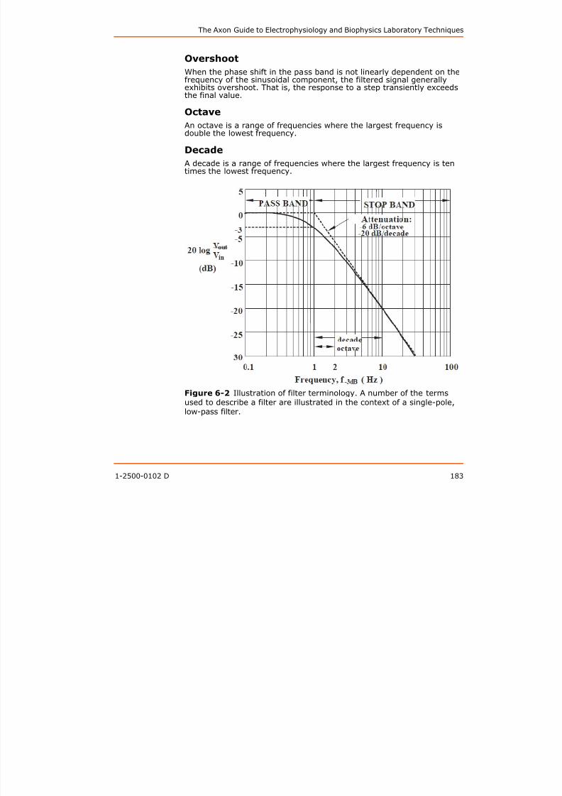
8/13/2019 User Guide v3
http://slidepdf.com/reader/full/user-guide-v3 184/302
1-2500-0102 D 183
Figure 6-2 Illustration of filter terminology. A number of the terms
used to describe a filter are illustrated in the context of a single-pole,low-pass filter.
Signal Conditioning and Signal Conditioners
Decibels (dB)
Since filters span many orders of magnitude of frequency andamplitude, it is common to describe filter characteristics usinglogarithmic terminology. Decibels provide the means of stating ratios oftwo voltages or two powers.
Voltage:
Thus, 20 dB corresponds to a tenfold increase in the voltage.
-3 dB corresponds to a √ 2 decrease in the voltage.
Power:
Thus, 10 dB corresponds to a tenfold increase of the power.
-3 dB corresponds to a halving of the power.
Some useful values to remember:

8/13/2019 User Guide v3
http://slidepdf.com/reader/full/user-guide-v3 185/302
184 1-2500-0102 D
Some useful values to remember:
Decibels Voltage Ratio Power Ratio
3 dB 1.414:1 2:1
6 dB 2:1 4:1
20 dB 10:1 100:1
40 dB 100:1 10,000:1
60 dB 1,000:1 1,000,000:1
66 dB 2,000:1 4,000,000:1
72 dB 4,000:1 16,000,000:1
80 dB 10,000:1 108:1
100 dB 100,000:1 1010:1
120 dB 1,000,000:1 1012:1
The Axon Guide to Electrophysiology and Biophysics Laboratory Techniques
Order
As mentioned above, the order of a filter describes the number ofpoles. The order is often described as the slope of the attenuation inthe stop band, well above f -3, so that the slope of the attenuation hasapproached its asymptotic value (Figure 6-2). Each row in the followingtable contains different descriptions of the same order filter.
Typically, the higher the order of the filter, the less the attenuation inthe pass band. That is, the slope of the filter in the pass band is flatterfor higher order filters (Figure 6-3).
Pole Order Slopes
1 pole 1st order 6 dB/octave 20 dB/decade
2 poles 2nd order 12 dB/octave 40 dB/decade
4 poles 4th order 24 dB/octave 80 dB/decade
8 poles 8th order 48 dB/octave 160 dB/decade

8/13/2019 User Guide v3
http://slidepdf.com/reader/full/user-guide-v3 186/302
1-2500-0102 D 185
Figure 6-3 Difference between a 4th- and 8th-order transfer function.
Signal Conditioning and Signal Conditioners
10-90% RISE TIME
The 10-90% rise time (t10-90) is the time it takes for a signal to risefrom 10% of its final value to 90% of its final value. For a signal passingthrough a low-pass filter, t10-90 increases as the -3 dB frequency of thefilter is lowered. Generally, when a signal containing a step changepasses through a high-order filter, the rise time of the emerging signalis given by:
For example, if f -3 is 1 kHz, t10-90 is approximately 300 μs.
As a general rule, when a signal with t10-90 = ts is passed through a filterwith t10-90 = tf , the rise time of the filtered signal is approximately:
Filtering for Time-Domain Analysis
Time-domain analysis refers to the analysis of signals that arerepresented the same way they would appear on a conventionaloscilloscope. That is, steps appear as steps and sine waves appear as

8/13/2019 User Guide v3
http://slidepdf.com/reader/full/user-guide-v3 187/302
186 1-2500-0102 D
oscilloscope. That is, steps appear as steps and sine waves appear assine waves. For this type of analysis, it is important that the filtercontributes minimal distortion to the time course of the signal. It wouldnot be very helpful to have a filter that was very effective at eliminatinghigh-frequency noise if it caused 15% overshoot in the pulses. Yet this iswhat many kinds of filters do.
In general, the best filters to use for time-domain analysis are Besselfilters because they add less than 1% overshoot to pulses. The Besselfilter is sometimes called a “linear-phase” or “constant delay” filter. Allfilters alter the phase of sinusoidal components of the signal. In aBessel filter, the change of phase with respect to frequency is linear. Put
differently, the amount of signal delay is constant in the pass band. Thismeans that pulses are minimally distorted. Butterworth filters addconsiderable overshoot: 10.8% for a fourth-order filter; 16.3% for aneighth-order filter. The step response of the Bessel and Butterworthfilters is compared in Figure 6-4.
The Axon Guide to Electrophysiology and Biophysics Laboratory Techniques
Figure 6-4 Step response comparison between bessel and butterworthfilters. The overshoots of fourth-order Bessel and Butterworth filters
d

8/13/2019 User Guide v3
http://slidepdf.com/reader/full/user-guide-v3 188/302
1-2500-0102 D 187
are compared.
In many experiments in biology and physiology (for example,voltage-and patch-clamp experiments), the signal noise increasesrapidly with bandwidth. Therefore, a single-pole filter is inadequate. Afour-pole Bessel filter is usually sufficient, but eight-pole filters are notuncommon. In experiments where the noise power spectral density isconstant with bandwidth (for example, recording from a strain gauge),a single-pole filter is sometimes considered to be adequate.
In the time domain, a notch filter must be used with caution. If therecording bandwidth encompasses the notch filter frequency, signals
that include a sinusoidal component at the notch frequency will begrossly distorted, as shown in Figure 6-5. On the other hand, if thenotch filter is in series with a low-pass or high-pass filter that excludesthe notch frequency, distortions will be prevented. For example, notchfilters are often used in electromyogram (EMG) recording in which theline-frequency pickup is sometimes much larger than the signal. The 50or 60 Hz notch filter is typically followed by a 300 Hz high-pass filter.The notch filter is required because the high-pass filter does notadequately reject the 50 or 60 Hz hum (Figure 6-5).

8/13/2019 User Guide v3
http://slidepdf.com/reader/full/user-guide-v3 189/302
The Axon Guide to Electrophysiology and Biophysics Laboratory Techniques
Filtering for Frequency-Domain Analysis
Frequency-domain analysis refers to the analysis of signals that areviewed to make a power spectrum after they are transformed into thefrequency domain. This is typically achieved using a fast Fouriertransform (FFT). After transformation, sine waves appear as thin peaksin the spectrum and square waves consist of their component sinewaves. For this type of analysis it does not matter if the filter distortsthe time-domain signal. The most important requirement is to have asharp filter cutoff so that noise above the -3 dB frequency does not getfolded back into the frequency of interest by the aliasing phenomenon(see Chapter 11: Noise in Electrophysiological Measurements onpage 259).
The simplest and most commonly used filter for frequency-domainanalysis in biological applications is the Butterworth filter. This filtertype has “maximally flat amplitude” characteristics in the pass band. Alllow-pass filters progressively attenuate sinusoidal components of thesignal as the -3 dB frequency is approached from DC. In a Butterworthfilter, the attenuation in the pass band is as flat as possible withouthaving pass-band ripple. This means that the frequency spectrum isminimally distorted.
Usually, notch filters can be safely used in conjunction withfrequency-domain analysis since they simply remove a narrow sectionof the power spectrum Nevertheless they are not universally used this

8/13/2019 User Guide v3
http://slidepdf.com/reader/full/user-guide-v3 190/302
1-2500-0102 D 189
of the power spectrum. Nevertheless, they are not universally used thisway because many experimenters prefer to record the data “as is” and
then remove the offending frequency component from the powerspectrum digitally.
Sampling Rate
If one intends to keep the data in the time domain, sufficient samplesmust be taken so that transients and pulses are adequately sampled.The Nyquist Sampling Theorem states that a bare minimum samplingrate is twice the signal bandwidth; that is, the -3 dB frequency of the
low-pass filter must be set at one half the sampling rate or lower.Therefore, if the filter -3 dB frequency is 1 kHz, the sampling theoremrequires a minimum sampling rate of 2 kHz. In practice, a significantlyhigher sampling rate is often used because it is not practical toimplement the reconstruction filters that would be required toreconstruct time-domain data acquired at the minimum sampling rate.A sampling rate of five or more times the -3 dB frequency of the filter iscommon.
If you wish to make peak-to-peak measurements of your data for
high-frequency signals, you must consider the sampling rate closely.The largest errors occur when samples are equally spaced around thetrue peak in the record. This gives the worst estimate of the peakvalue. To illustrate the magnitude of this problem, assume that thesignal is a sine wave and that the following number of samples are
Signal Conditioning and Signal Conditioners
taken per cycle of the sine wave. The maximum errors that one couldget are then as follows:
The sampling of the peak values varies between no error and themaximum as stated above.
If one intends to transform the data into the frequency domain,Butterworth or Elliptic filters are more suitable than the Bessel filter.These filters have a sharper cutoff near the -3 dB frequency than theBessel filter, and thus better prevent the phenomenon known asaliasing. With a fourth-order or higher Butterworth filter, it is usual to
set f -3 to about 40% of the sampling rate. Frequently, researchers donot have a Butterworth filter handy. If a Bessel filter is available, it canbe used instead, but f -3 would normally be set to about 25–30% of thesampling rate. This is because the Bessel filter attenuation is not assharp near the -3 dB frequency as that of a Butterworth filter.
Filtering Patch-Clamp Data
The analog filters that are typically used with a patch clamp are the
5 samples/cycle 19.0% error
10 samples/cycle 4.9% error
20 samples/cycle 1.2% error

8/13/2019 User Guide v3
http://slidepdf.com/reader/full/user-guide-v3 191/302
190 1-2500-0102 D
The analog filters that are typically used with a patch clamp are theBessel and Butterworth types, in either 4-pole or 8-pole versions. If
simply regarded from the noise point of view, the Butterworth filter isthe best. Empirical measurements carried out by Molecular Devicesreveal that the rms noise passed by the filters (relative to a 4-poleBessel filter) when used with an Axopatch™ 200 amplifier in single-channel patch mode is as follows:
The table shows that the main reduction in noise is gained by using aButterworth filter instead of a Bessel filter. The improvement achievedby going from a 4-pole filter to an 8-pole filter of the same kind issmall.
However, for the reasons previously discussed above, the Butterworthfilter cannot be used for time-domain analysis. Since this is the mostcommon kind of analysis performed on patch-clamp data, Bessel filtersare almost invariably used.
Noise4-PoleBessel
8-PoleBessel
4-PoleButterworth
8-PoleButterworth
1 kHz 1.0 0.97 0.95 0.93
5 kHz 1.0 0.97 0.85 0.82
10 kHz 1.0 0.94 0.83 0.80
The Axon Guide to Electrophysiology and Biophysics Laboratory Techniques
Digital Filters
Some researchers prefer to record data at wide bandwidths to preventthe loss of potentially important information. An analog filter is used toprovide anti-alias filtering, followed by a digital filter implemented atvarious lower -3 dB frequencies during the analysis. There are manytypes of digital filters. Two types are described here:
Nonrecursive Filter
The output of a nonrecursive filter depends only on the input data.There is no dependence on the history of previous outputs. An exampleis the smoothing-by-3’s filter:
where yn and xn are the output and input samples at sample interval n.Nonrecursive filters are also known as “finite impulse response” filters(FIR) because their response to a single impulse endures only as longas the newest sample included in the formula (for example, xn+1 in thesmoothing-by-3’s filter).
Another example of a nonrecursive digital filter is the Gaussian filter. Ithas a similar form to the smoothing-by-3’s filter described above,except that typically there are more terms and the magnitudes of the

8/13/2019 User Guide v3
http://slidepdf.com/reader/full/user-guide-v3 192/302
1-2500-0102 D 191
except that typically there are more terms and the magnitudes of thecoefficients lie on the bell-shaped Gaussian curve.
These types of filters have the advantage of not altering the phase ofthe signal. That is, the mid-point for the rise time of a step occurs atthe same time both before and after filtering. In contrast, analog filtersalways introduce a delay into the filtered signal.
A problem with digital filters is that values near the beginning and endof the data cannot be properly computed. For example, in the formulaabove, if the sample is the first point in the data, xn-1 does not exist.This may not be a problem for a long sequence of data points; however,
the end effects can be serious for a short sequence. There is no goodsolution other than to use short filters (for example, few terms). Addingvalues outside the sequence of data is arbitrary and can lead tomisleading results.
Recursive Filter
The output of a recursive filter depends not only on the inputs, but onthe previous outputs as well. That is, the filter has sometime-dependent “memory.” Recursive filters are also known as “infinite
impulse response” filters (IIR) because their response to a singleimpulse extends indefinitely into the future (subject to computerprocessing limitations).
Digital-filter implementations of analog filters such as the Bessel,Butterworth, and RC filters are recursive.
Signal Conditioning and Signal Conditioners
Correcting for Filter Delay
The delay introduced by analog filters necessarily makes recordedevents appear to occur later than they actually occurred. If it is notaccounted for, this added delay can introduce an error in subsequentdata analysis. The effect of the delay can be illustrated by consideringtwo common questions: How long after a stimulus did an event occur(latency measurement)? And, what was the initial value of anexponentially decaying process (extrapolation back to the zero time ofa fitted curve)? If the computer program was instructed to record 50points of baseline and then apply a stimulus, it would be natural, butincorrect, to assume in the subsequent analysis that zero time beginssomewhere between points 50 and 51 of the recorded data, since zerotime may actually be at point 52 or later.
The delay can be seen in Figure 6-4. The times to the 50% rise or fallpoint of a step signal (delay) are approximately 0.33/f -3 for a
fourth-order low-pass Bessel filter, and 0.51/f -3 for an eighth-orderBessel filter. In practice, when using a fourth-order Bessel filter withf -3 = 1 kHz and sampling the trace at 6 kHz, the filter delay is 330 μs.So, the whole record will have to be shifted by 2.0 points with respectto the stimulus events that were programmed.
Preparing Signals for A/D Conversion

8/13/2019 User Guide v3
http://slidepdf.com/reader/full/user-guide-v3 193/302
192 1-2500-0102 D
Analog-to-Digital (A/D) converters have a fixed resolution and measuresignals in a grainy manner. This means that all signals lying betweencertain levels are converted as if they are the same value. To minimizethe impact of this undesirable “quantization” effect, it is important toamplify the signal prior to presenting it to the A/D converter. Ideally,the gain should be chosen so that the biggest signals of interest occupythe full range of the A/D converter but do not exceed it. In mostlaboratory systems, the full range of the A/D converter is ±10 V, butother ranges such as ±5 V and ±1.25 V are often used in industrialapplications.
Where to Amplify
Amplification is possible at a number of different points along the signalpathway. Since the amplification, filtering and offset circuits canthemselves introduce noise, the location of the amplification circuitrymust be carefully considered. There are several options:
Inside the Recording Instrument
The ideal place to amplify the signal is inside the instrument thatrecords the signal. For example, the Axopatch 200B, MultiClamp 700B,and Axoclamp™ 900A amplifiers from Molecular Devices contain avariable gain control in the output section that can be used to providelow-noise amplification of the pipette current or membrane potential.
The Axon Guide to Electrophysiology and Biophysics Laboratory Techniques
The advantage of placing the amplification inside the recordinginstrument is that the amount of circuitry between the low-level signaland the amplifying circuitry can be minimized, thereby reducingextraneous noise contributions.
Between the Recording Instrument and the A/D Converter
A good place to amplify the signal is after it emerges from the recordinginstrument, before it is sent to the A/D converter. The CyberAmp® 380amplifier from Molecular Devices can be used for this purpose. For thebest noise performance, a small amount of initial amplification shouldbe provided in the recording instrument if the signal levels are low. Themain advantage of using a multi-channel amplifier such as theCyberAmp is that the gain of each recording pathway can beindependently set by the computer. An instrument such as theCyberAmp amplifier has more gain choices than are usually available in
a recording instrument.In either of the examples discussed so far, anti-aliasing filtering isconveniently provided on a per-channel basis after the gainamplification.
After the Channel Multiplexor on the A/D Converter Board
A common place to provide amplification is in a programmable gainamplifier (PGA) located after the channel multiplexor on the A/D

8/13/2019 User Guide v3
http://slidepdf.com/reader/full/user-guide-v3 194/302
1-2500-0102 D 193
p ( ) pconverter board. Briefly, in the A/D converter board, many channels are
typically digitized by a single A/D converter. The signals aresequentially presented to the A/D converter by a multiplexor circuit. APGA located after the multiplexor is very economical, since only onePGA is required regardless of the number of channels.
The main advantage of locating a PGA after the multiplexor on the A/Dboard is that it is inexpensive. However, there are significantdisadvantages:
1. The PGA has to have extremely wide bandwidth since it must beable to settle within the resolution of the A/D converter at themultiplexing rate. Depending on the number of channels beingsampled, this could mean that the bandwidth of the PGA has tobe ten to several hundred times greater than the bandwidth ofthe analog signals. Such fast amplifiers are difficult to design,but in many cases the required speed can be achieved. The lessobvious problem is that every amplifier introduces intrinsicnoise, and the amount of noise observed on the amplifier outputincreases with bandwidth. Since the PGA may have severalhundred times more bandwidth than the analog signal, it is
likely to contribute more noise to the recording than is inherentin the signal. This problem cannot be eliminated or evenreduced by filtering because filtering would lengthen the settlingtime of the PGA. This serious problem limits the usefulness of ashared PGA. This problem does not exist in the previously
Signal Conditioning and Signal Conditioners
discussed systems in which there is an amplifier for eachchannel.
2. If the PGA is located on the A/D board, the low-level signalsmust be brought by cables to the A/D board. Typically, thesecables are a couple of meters or more in length and provideample opportunity for pick up of hum, radio-frequency
interference, and cross-talk between signals. With carefulattention to shielding and grounding, these undesirable effectscan be minimized. In the alternative approaches, in which thesignals are amplified before they are sent to the A/D converter,the relative impact of these undesirable interferences arereduced in proportion to the amount of early amplification.
Systems that include a PGA on the A/D board are useful when thesignals require only a small amount of amplification (ten fold or less) orwhen the user cannot afford or has not invested in external amplifiers.
Pre-Filter vs. Post-Filter Gain
When low-level signals are recorded, it is essential that the first-stageamplification be sufficient to make the noise contributed by succeedingstages irrelevant. For example, in a microphone amplifier the tinyoutput from the microphone is first coupled into an extremely low-noisepre-amplifier. After this first-stage amplification, circuits with moremodest noise characteristics are used for further amplification and to
d bl d b f l

8/13/2019 User Guide v3
http://slidepdf.com/reader/full/user-guide-v3 195/302
194 1-2500-0102 D
introduce treble and bass filtering.
If the only rule was to maximize the early gain, all of the gain would beimplemented before any low-pass filter, notch filter or offset stages.However, with some signals, too much gain in front of the low-passfilter can introduce a different problem. This occurs when the signal ismuch smaller than the out-of-band noise.
This problem is illustrated by the signal in Figure 6-6. Panel A shows aninput signal consisting of a pair of 1 pA current pulses significantlycorrupted by instrumentation noise. When the noisy signal is first
amplified by x100 and then low-pass filtered, the amplified noisy signalsaturates the electronics and the noise is clipped. (Note that for clarity,these traces are not drawn to scale.) After low-pass filtering, the signallooks clean, but its amplitude is less than x100 the original signalbecause the low-pass filter extracts a signal that is the average of thenon-symmetrical, clipped noise. When the noisy signal is first amplifiedby x10, then low-pass filtered before a further amplification by x10,saturation is avoided and the amplitude of the filtered signal is x100 theoriginal input. Panel B shows the two outputs superimposed to illustratethe loss of magnitude in the signal that was amplified too much before
it was low-pass filtered.
The Axon Guide to Electrophysiology and Biophysics Laboratory Techniques
Figure 6-6 Distortion of signal caused by high amplification prior tofiltering

8/13/2019 User Guide v3
http://slidepdf.com/reader/full/user-guide-v3 196/302
1-2500-0102 D 195
filtering.
Offset Control
In some cases, it is necessary to add an offset to the signal before it isamplified. This is necessary if the gain required to amplify the signal ofinterest would amplify the DC offset of the signal to the point that itwould cause the gain amplifier to saturate.
An example is provided by an electronic thermometer. A typicalsensitivity of an electronic thermometer is 10 mV/°C, with zero volts
corresponding to 0°C. A 12-bit A/D converter can measure with anapproximate resolution of 5 mV, corresponding to 0.5°C in thisexample. If the data are to be analyzed at 0.01°C resolution,amplification by a factor of at least x50, and probably x100, would benecessary. If the temperatures of interest are between 30°C and 40°Cand are amplified by x100, these temperatures will correspond tovoltages between 30 V and 40 V values well beyond the range of theA/D converter. The solution is to introduce an offset of -350 mV beforeany amplification, so that zero volts will correspond to 35°C. Now whenthe signal is amplified by x100, the 30–40°C temperature range willcorrespond to voltages between -5 V and +5 V.
Signal Conditioning and Signal Conditioners
AC Coupling and Autozeroing
AC coupling is used to continuously remove DC offsets from the inputsignal. Signals below the -3 dB frequency of the AC coupling circuit arerejected. Signals above this frequency are passed. For this reason, ACcoupling circuits are more formally known as high-pass filters. In mostinstruments with AC coupling, the AC coupling circuit is a first-order
filter. That is, the attenuation below the -3 dB frequency increases at20 dB/decade.
When a signal is AC coupled, the DC component of the signal iseliminated and the low-frequency content is filtered out. This causessignificant distortion of the signal, as shown in Figure 6-7.

8/13/2019 User Guide v3
http://slidepdf.com/reader/full/user-guide-v3 197/302
196 1-2500-0102 D
Figure 6-7 Distortion of signal caused by AC-coupling at highfrequencies.
A 1 Hz square wave is AC-coupled at three different frequencies. Thedistortion is progressively reduced as the AC-coupling frequency isreduced from 10 Hz to 0.1 Hz. In all cases, the DC content of the signal
is removed. The problem when using the lowest AC-couplingfrequencies is that slow shifts in the baseline may not be rejected andtransient shifts in the baseline might take a long time to recover.
Since there is less distortion when the AC-coupling frequency is lower, itis tempting to suggest that the AC-coupling should always be set to
The Axon Guide to Electrophysiology and Biophysics Laboratory Techniques
very low frequencies, such as 0.1 Hz. However, this is oftenunacceptable because some shifts in the baseline are relatively rapidand need to be eliminated quickly.
A significant difference between using an AC coupling circuit and settinga fixed DC offset is the way the two circuits handle ongoing drift in thesignal. With fixed DC offset removal, the ongoing drift in the signal is
recorded. With AC coupling, the drift is removed continuously. Whetherthis is an advantage or a disadvantage depends on whether the drifthas meaning.
For very slow signals, even the lowest AC-coupling frequency causessignificant distortion of the signal. For these signals, an alternativetechnique known as autozeroing can be used. This technique isavailable in some signal conditioners, such as the CyberAmp 380amplifier, as well as in some amplifiers, such as the Axopatch-1amplifier. In this technique, the signal is DC-coupled and a sample of
the signal is taken during a baseline period. This DC sample value isstored and continuously subtracted by the instrument from the signaluntil the next sample is taken. In early instruments, the sample wastaken using an analog sample-and-hold circuit. These circuits exhibitthe problem known as “droop.” That is, the sampled value drifts withtime. Later systems, such as the ones used in the CyberAmp 380amplifier, use droop-free, digital sample-and-hold circuits.
The efficacy of the technique is illustrated in Figure 6-8.

8/13/2019 User Guide v3
http://slidepdf.com/reader/full/user-guide-v3 198/302
1-2500-0102 D 197
Signal Conditioning and Signal Conditioners

8/13/2019 User Guide v3
http://slidepdf.com/reader/full/user-guide-v3 199/302
198 1-2500-0102 D
Figure 6-8 Comparison of autozeroing to AC-coupling.
The top trace shows an EKG signal that is sitting on a 5 mV offsetresulting from electrode junction potentials. At AC-coupling frequenciesof 10 Hz and 1 Hz, the signal is distorted. In the bottom trace, anAutozero command is issued to the signal conditioner (the CyberAmp380 amplifier) at the time indicated by the arrow. The DC component isimmediately removed, but the transients are unaffected. Autozeroingshould be restricted to cases where the time of occurrence of signals is
known, so that the Autozero command can be issued during thebaseline recording period preceding the signal.
Time Constant
The AC-coupling frequency is related to the time constant of decay, τ (Figure 6-7):

8/13/2019 User Guide v3
http://slidepdf.com/reader/full/user-guide-v3 200/302
Signal Conditioning and Signal Conditioners
such as the CyberAmp amplifier, the host computer can interrogate theCyberAmp amplifier to determine if an overload has occurred.
Averaging
Averaging is a way to increase the signal-to-noise ratio in those cases
where the frequency spectrum of the noise and the signal overlap. Inthese cases, conventional filtering does not help because if the -3 dBfrequency of the filter is set to reject the noise, it also rejects thesignal.
Averaging is applicable only to repetitive signals, when many sweeps ofdata are collected along with precise timing information to keep track ofthe exact moment that the signal commences or crosses a threshold.All of these sweeps are summed, then divided by the total number ofsweeps (N) to form the average. Before the final division, the amplitude
of the signal in the accumulated total will have increased by N. Becausethe noise in each sweep is uncorrelated with the noise in any of theother sweeps, the amplitude of the noise in the accumulated signal willonly have increased by √ N. After the division, the signal will have amagnitude of unity, whereas the noise will have a magnitude of 1/ √ N.Thus, the signal-to-noise ratio increases by √ N.
Line-frequency Pick-up (Hum)

8/13/2019 User Guide v3
http://slidepdf.com/reader/full/user-guide-v3 201/302
200 1-2500-0102 D
An important consideration when measuring small biological signals isto minimize the amount of line-frequency pickup, often referred to ashum. Procedures to achieve this goal by minimizing the hum at itssource are discussed in Chapter 2: The Laboratory Setup on page 39.
Hum can be further minimized by using a notch filter, as discussedabove, or by differential amplification. To implement the lattertechnique, the input amplifier of the data acquisition system isconfigured as a differential amplifier. The signal from the measurement
instrument is connected to the positive input of the differentialamplifier, while the ground from the measurement instrument isconnected to the negative input. If, as is often the case, the hum signalhas corrupted the ground and the signal equally, the hum signal will beeliminated by the differential measurement.
Peak-to-Peak and RMS Noise Measurements
Noise is a crucially important parameter in instruments designed formeasuring low-level signals.
Invariably, engineers quote noise specifications as root-mean-square(rms) values, whereas users measure noise as peak-to-peak (p-p)values. Users’ preference for peak-to-peak values arises from the fact
The Axon Guide to Electrophysiology and Biophysics Laboratory Techniques
that this corresponds directly to what they see on the oscilloscopescreen or data acquisition monitor.
Engineers prefer to quote rms values because these can be measuredconsistently. The rms is a parameter that can be evaluated easily. Instatistical terms, it is the standard deviation of the noise. True rmsmeters and measurement software are commonly available and the
values measured are completely consistent.On the other hand, peak-to-peak measurements are poorly defined andno instruments or measurement software are available for theirdetermination. Depending on the interpreter, estimates of thepeak-to-peak value of Gaussian noise range from four to eight timesthe rms value. This is because some observers focus on the “extremes”of the noise excursions (hence, the x8 factor), while others focus on the “reasonable” excursions (x6 factor) or the “bulk” of the noise (x4factor).
Molecular Devices has developed the pCLAMP® software to measure therms and the peak-to-peak noise simultaneously. The peak-to-peaknoise is calculated as the threshold level that would encompass acertain percentage of all of the acquired data. For white noise, thecorresponding values are:
Percentage of DataEncompassed
Peak-To-PeakThresholds

8/13/2019 User Guide v3
http://slidepdf.com/reader/full/user-guide-v3 202/302
1-2500-0102 D 201
These empirical measurements can be confirmed by analysis of theGaussian probability distribution function.
In this guide and various Axon Conventional Electrophysiology productspecifications, noise measurements are usually quoted in both rms and
peak-to-peak values. Since there is no commonly accepted definition ofpeak-to-peak values, Molecular Devices usually uses a factor of about 6to calculate the peak-to-peak values from the measured rms values.
In an article from Bell Telephone Laboratories (1970), the authorsdefine the peak factor as “the ratio of the value exceeded by the noise acertain percentage of the time to the rms noise value. This percentageof time is commonly chosen to be 0.01 per cent.” This ratio, from tableslisting the area under the Gaussian distribution, turns out to be 7.78times the rms value. Thus, according to this article, the appropriate
factor to calculate the peak-to-peak values from the measured rmsvalues is closer to x8.
95.0% 3.5–4 times rms value99.0% 5–6 times rms value
99.9% 7–8 times rms value
Signal Conditioning and Signal Conditioners
Blanking
In certain experiments, relatively huge transients are superimposed onthe signal and corrupt the recording. This problem commonly occursduring extracellular recording of nerve impulses evoked by ahigh-voltage stimulator. If the isolation of the stimulator is not perfect(it never is), there is some coupling of the stimulus into themicropipette input. This relatively large artifact can sometimes causethe coupling capacitors in subsequent AC amplifiers to saturate. Theremight be some time lost while these capacitors recover from saturation,and thus valuable data might be wasted.
If it is not possible to prevent the stimulus coupling, the next best thingto do is to suppress the artifact before it feeds into the AC-coupledamplifiers. This is made possible in the Axoclamp 900A amplifier byproviding sample-and-hold amplifiers early in the signal pathway. Theuser provides a logic-level pulse that encompasses the period of thetransient. This logic-level pulse forces the sample-and-hold amplifiersinto the “hold” mode. In this mode, signals at the input of thesample-and-hold amplifier are ignored. Instead, the output of thesample-and-hold amplifier is kept equal to the signal that existed at themoment the logic-level pulse was applied.
Audio Monitor: Friend or Foe?

8/13/2019 User Guide v3
http://slidepdf.com/reader/full/user-guide-v3 203/302
202 1-2500-0102 D
When monitoring data, experimenters need not be limited to theirsense of sight. The data may also be monitored with great sensitivityusing the sense of hearing. In such cases, the data are input to anaudio monitor and fed to a loudspeaker or a set of headphones.
Two types of audio monitor are used. The first is a power amplifier thatapplies the signal directly to the speaker, thereby allowing signals in theaudio bandwidth to be heard. This type of audio monitor is frequentlyused in EMG monitoring or in central nervous system recording. Eachspike is heard as an audible click, and the rate and volume of clicking is
a good indicator of the muscle or nerve activity. This type of audiomonitor is either called an AM (amplitude modulated) audio monitor, orit is said to be operating in “click” mode.
The second type of audio monitor is a tone generator whose frequencydepends on the amplitude of the input signal. Usually, the oscillatorfrequency increases with increasingly positive signals. This type ofaudio monitor is often used for intracellular recording. It provides anextremely sensitive measure of the DC level in the cell. This type ofaudio monitor is either called an FM (frequency modulated) audio
monitor, or it is said to be operating in “tone” mode.
The Axon Guide to Electrophysiology and Biophysics Laboratory Techniques
Most researchers have a very strong opinion about audio monitors;they either love them or hate them. Those who love audio monitorsappreciate the supplementary “view” of the data. Those who hate audiomonitors have probably suffered the annoyance of having to listen forinterminable lengths of time to the audio output from another rig in thesame room. A constant tone can be irritating to listen to, especially if itis high pitched, unless it has an important message for you, such as
“my cell is maintaining its potential admirably.” Audio monitors are standard features in Axon ConventionalElectrophysiology computer controlled amplifiers. To minimize thepotential for aggravation, we include a headphone jack so that userscan listen to the audio output without testing the patience of theircolleagues.
Electrode Test
It is useful to be able to measure the electrode resistance for tworeasons. The first reason is to establish the basic continuity of theelectrode circuit. Sometimes, electrode leads can break, leaving anopen-circuit input and, consequently, no incoming data. The secondreason is to verify that the electrode is acceptably attached. Forexample, it may be that to achieve the low-noise recording levelsneeded in an EMG recording, the electrode resistance must be less than5 kΩ.
d l f ll h l d d b l

8/13/2019 User Guide v3
http://slidepdf.com/reader/full/user-guide-v3 204/302
1-2500-0102 D 203
Some transducer amplifiers allow the electrode impedance to be easilymeasured. For example, the CyberAmp amplifiers have an ElectrodeTest facility. When this is activated, an approximate 1 μAp-p, 10 Hzsquare wave is connected to every input via individual 1 MΩ resistors.The electrode resistance can be directly determined from the amplitudeof the voltage response.
Common-Mode Rejection Ratio
In general, the information that the researcher wants to record is thedifference between two signals connected to the positive and thenegative amplifier inputs. Often, these signals contain an additionalcomponent that is common to both, but that does not contain relevantinformation. For example, both outputs of a strain gauge might includea DC potential of 2.5 V that arises from the excitation voltage.However, the strain on the gauge generates a microvolt-size differencebetween the two outputs, but does not affect the 2.5 V “common-mode” voltage. Another example is often seen when
recording EMG signals from an animal. Both the positive and thenegative electrodes pick up line-frequency hum that has coupled intothe animal. The hum picked up by the electrodes may be as large as10 mV, but it is identical on both electrodes. The EMG signal of interest
Signal Conditioning and Signal Conditioners
is the small difference between the potentials on the two electrodes; itmay be as small as a few tens of microvolts.
To prevent the common-mode signal from swamping the much smallerdifferential signal, the positive and negative gains of the amplifier mustbe nearly identical. In the above EMG example, if the amplifier inputsare exactly unity, the 10 mV of hum that appears equally on both
electrodes does not show up at all on the amplifier output. The onlysignal to appear on the output is the small signal proportional to theEMG potential generated between the two electrodes.
In practice, the positive and negative inputs of the amplifier are neverexactly equal. The quality of their matching is measured by thecommon-mode rejection ratio (CMRR). This is normally quoted in dB,where 20 dB corresponds to a factor of ten. Returning to the EMGexample, if the amplifier operates at unity gain with a CMRR of 60 dB(for example, one part in a thousand), the 10 mV of common-mode
hum results in 10 μV of hum appearing on the amplifier output. This issmall, but still significant compared with the smallest EMG signals, soan amplifier with higher CMRR, for example, 80 dB, may be desirable.
The CMRR of an amplifier varies with frequency. It is best at very lowfrequencies, while above a certain frequency it diminishes steadily asthe frequency of the common-mode signal increases. It is thereforeimportant to verify the CMRR of the amplifier at a frequency thatexceeds the expected frequency of the common-mode signal.
The CMRR of the recording system is adversely affected by imbalances
i th i t f th di l t d Thi i b

8/13/2019 User Guide v3
http://slidepdf.com/reader/full/user-guide-v3 205/302
204 1-2500-0102 D
in the source resistances of the recording electrodes. This is becausethe source resistance of each electrode forms a voltage divider with theinput resistance of the amplifier. If the source resistances of the twoelectrodes are not identical, the voltage dividers at the positive andnegative inputs of the amplifier are not equal. Returning to the EMGexample, if the resistance of one electrode is 9 kΩ, the resistance ofthe other is 10 kΩ, and the amplifier input resistances total 1 MΩ, thenthe gain for one electrode is 0.9901 instead of unity, while the gain forthe other electrode is 0.9911. The difference is 0.001. Thus, even
though the amplifier may have a CMRR of 80 dB or more, the systemCMRR is only 60 dB. In some cases, 60 dB is acceptable, but in others itis not. The solution to this problem is to use an amplifier that has veryhigh input resistances of 100 MΩ or more.
If there is a large common-mode signal and a source imbalance ofmore than a few kilohms, a high input resistance amplifier probe shouldbe used. Several AI 400 series probes are available from MolecularDevices that have input resistances of 10 gigohms (1010 Ω) or more.These probes are distinguished on the basis of noise, cost and size.
The Axon Guide to Electrophysiology and Biophysics Laboratory Techniques
References
Bell Telephone Laboratories. Transmission Systems forCommunications. By the members of the technical staff at BellTelephone Laboratories. Western Electric Company, Inc., TechnicalPublications. Winston-Salem, North Carolina, 1970.
Further Reading
Hamming, R. W., Digital Filters. Prentice-Hall, Inc., Englewood Cliffs,New Jersey, 1977.
Tietze, U., Schenk, Ch., Advanced Electronic Circuits. Springer-Verlag,Berlin, 1978.

8/13/2019 User Guide v3
http://slidepdf.com/reader/full/user-guide-v3 206/302
1-2500-0102 D 205
Signal Conditioning and Signal Conditioners

8/13/2019 User Guide v3
http://slidepdf.com/reader/full/user-guide-v3 207/302
206 1-2500-0102 D
7Transducers
Transducers are devices that convert a signal of one form to another. In
physiological applications this usually means converting variations of aphysical signal, such as temperature or pressure, into variations involtage that can then be recorded or manipulated as necessary.
There are many different types of transducers available forphysiological recording and they range in their requirements forexcitation voltages, amplification, and recording techniques as well asmechanical connections. In the past this has required a differentamplifier for each transducer type. The introduction of the CyberAmp® 380 amplifier (Molecular Devices), a computer-controlled signal-conditioning amplifier, heralded a new approach to interfacingtransducers. A small 15-pin socket on each channel of the CyberAmp380 amplifier provides the excitation voltage, the differential inputs,the offset correction and the filtering required by a wide variety oftransducers. This eliminates the need for a dedicated amplifier to suitthe transducer type. The AI 400 series probes and adapters can pluginto any socket on the CyberAmp 380 amplifier. Within the 15-pin probeconnector is a small memory device called an EEPROM (electricallyerasable programmable read only memory) that stores suchinformation as the transducer type, its scale factor and the offset.
When the transducer is plugged into the CyberAmp 380 amplifier thisi f ti b t ti ll l d d b th i iti ft

8/13/2019 User Guide v3
http://slidepdf.com/reader/full/user-guide-v3 208/302
1-2500-0102 D 207
When the transducer is plugged into the CyberAmp 380 amplifier, thisinformation may be automatically loaded by the acquisition software,thereby making the transducer ready for immediate use.
Temperature Transducers for Physiological TemperatureMeasurement
Three types of transducers are suitable for physiological temperature
measurement: thermistors, integrated circuit (IC) temperaturetransducers that produce an output current proportional to absolutetemperature, and IC temperature transducers that produce an outputvoltage proportional to absolute temperature.
Thermistors
Thermistors are resistors whose resistance drops significantly astemperature increases. They are composed of a compressed and
sintered mixture of metallic oxides of manganese, nickel, cobalt,copper, magnesium, titanium and other metals. Thermistors exhibittemperature coefficients many times greater than those of pure metals.For most of them, the resistance falls by 4–6% per °C with increasingtemperature.
Transducers
The response is exponential with temperature, but can be considered tobe linear over a range of a few tens of degrees Celsius. By combiningmultiple thermistors and some resistors, the useful linear range can beextended to span more than 100°C. The Omega Engineering, Inc.(Stamford, CT) thermistor composites 44018 and 44019 each contain amatched pair of thermistors. When connected by precision resistors toan accurate DC excitation voltage, these probes are interchangeable
within ±0.15°C over the recommended range of -30 to +100°C. Theseprobes come in a wide range of shapes and sizes for differentapplications such as esophageal, rectal and surface body temperaturemeasurements, or for immersion in hostile chemical environments.
Omega Engineering Inc. produces many other thermistor types as doother manufacturers. These other types can also be interfaced to theCyberAmp 380 amplifier via the AI 490 Connector and AI 491 CableKits. Several different interface circuits are suggested in the CyberAmp380 manual.
IC Temperature Transducers That Produce an OutputCurrent Proportional to Absolute Temperature
The most notable of these temperature-dependent current sources arethe Analog Devices, Inc. (Norwood, MA) AD590 with a temperaturerange of -55 to +150°C and the lowercost AD592 with a temperaturerange of -25 to +105°C. These are not available in the wide range ofprobe configurations provided by thermistor manufacturers. Most often
they are supplied in 0.23” (5.8 mm) diameter metal cans or in 0.25” x0 093” (6 4 2 4 ) i fl t k Th d t b

8/13/2019 User Guide v3
http://slidepdf.com/reader/full/user-guide-v3 209/302
208 1-2500-0102 D
they are supplied in 0.23 (5.8 mm) diameter metal cans or in 0.25 x0.093” (6.4 mm x 2.4 mm) ceramic flat packs. These need to beconnected to wires and must be insulated for special purposes. Theonly temperature probe available from Analog Devices is the AC2626,which includes an AD590 enclosed in a 4” (102 mm) or 6” (153 mm)long stainless steel sheath with a 3/16” (4.8 mm) outside diameter.
When connected to a DC voltage source (for example, the +5 Vexcitation voltage in the CyberAmp 380 amplifier) these transducersforce the current that flows in the circuit to be equal to 1 μA/°K. The
external circuitry required to use the AD590 is very simple and it iseasy to configure for minimum and average temperaturemeasurements by placing transducers in series or in parallel,respectively. The absolute accuracy and interchangeability of theseprobes is inferior to the Omega Engineering probes described above. Intheir best and most expensive grade, the interchangeability is ±0.5°Cat 25°C. The main advantages of the AD590 temperature probes arethat the external support circuitry is very simple and that they aresuitable for remote sensing applications. Because the output is
insensitive to voltage drops, the devices can be used with twisted-paircabling hundreds of feet in length.
The Analog Devices semiconductor temperature probes can beinterfaced to the CyberAmp 380 amplifier via the AI 490 Connector andAI 491 Cable Kits, with the user providing the interface design based on
The Axon Guide to Electrophysiology and Biophysics Laboratory Techniques
the range of application circuits provided by Analog Devices and in themanual for the CyberAmp 380 amplifier.
IC Temperature Transducers That Produce an OutputVoltage Proportional to Absolute Temperature
Two of the most suitable temperature-dependent voltage sources arethe LM35A and the LM135A sensors from National SemiconductorCorporation (Santa Clara, CA). These have absolute accuracies(interchangeability) of ±0.5°C and ±1.0°C, respectively, at 25°C. TheLM35A has a zero voltage output at 0 °C and a sensitivity of 10 mV/°C.The LM135A behaves as a zener diode with a zero voltage output at 0°Cand a sensitivity of 10 mV/°C. These devices are generally cheaperthan the AD590 transducers. They are supplied in approximately 0.2”(5 mm) metal cans or plastic packages, but they are not available inready-to-use probes.
The National Semiconductor temperature probes can be interfaced tothe CyberAmp 380 amplifier via the AI 490 Connector and AI 491 CableKits with the user providing the interface design using the range ofapplication circuits provided by National Semiconductor and in themanual for the CyberAmp 380 amplifier.
Temperature Transducers for Extended
Temperature Ranges

8/13/2019 User Guide v3
http://slidepdf.com/reader/full/user-guide-v3 210/302
1-2500-0102 D 209
Temperature RangesTwo types of transducers are commonly used for temperaturemeasurements beyond the physiological range: thermocouples andresistance temperature detectors.
Thermocouples
Thermocouples are economical and rugged transducers, having theadvantage of small size with a very fast response time and a wide
temperature range. Thermocouples consist of two dissimilar metals incontact. The offset potential between the metals is proportional totemperature (see Table 7-1). The low sensitivity and broad operatingrange generally make thermocouples more suitable for industrialapplications than for physiological ones. Because of their greatersensitivity, thermistors are more popular than thermocouples for mostphysiological applications. On the other hand, thermocouples can befabricated in remarkably small sizes, creating the opportunity for someunusual biological applications. For example, micron-dimension
thermocouples that can be inserted into single living cells have beendescribed (Cain & Welch, 1974). Commercially available thermocouplescan be obtained with diameters as low as 25 μm and thermal timeconstants as short as 2 ms (Omega Engineering, Inc., Stamford, CT).
Transducers
Thermocouples require a reference temperature that traditionally wasan ice bath but is more commonly provided by a compensation circuit.Complete signal-conditioning modules, such as the Analog DevicesAD594 and 3B47 signal conditioners, exist. They contain the differentialamplifiers and the temperature compensation circuitry. Alternatively,voltage-output temperature transducers, such as the LM35A, can beused to derive a compensation voltage to apply to the negative input ofa CyberAmp 380 amplifier. To interface thermocouples to the CyberAmp380 amplifier, the user must provide an interface circuit using atemperature transducer for compensation or using the Analog Devices
i l t diti i d l Ci it l i i th
Table 7-1 Common Thermocouple Materials.
ANSIType
MinValue °C
MaxValue °C
Sensitivity at20°C μV/°C
Material
E -200 900 60.48 chromel/constantan
J -200 750 51.45 iron/constantanK -200 1250 40.28 chromel/alumel
R 0 1450 5.80 platinum/Pt-13%rhodium
S 0 1450 5.88 platinum/Pt-10%rhodium
T -200 350 40.28 copper-constantan
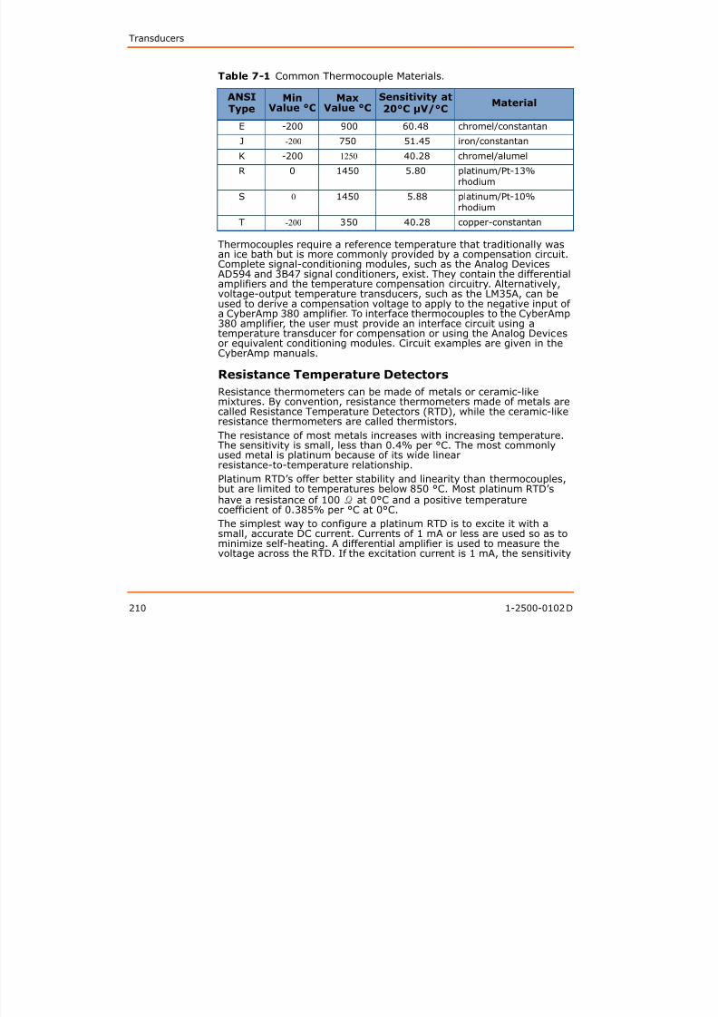
8/13/2019 User Guide v3
http://slidepdf.com/reader/full/user-guide-v3 211/302
210 1-2500-0102 D
or equivalent conditioning modules. Circuit examples are given in theCyberAmp manuals.
Resistance Temperature Detectors
Resistance thermometers can be made of metals or ceramic-likemixtures. By convention, resistance thermometers made of metals arecalled Resistance Temperature Detectors (RTD), while the ceramic-like
resistance thermometers are called thermistors.The resistance of most metals increases with increasing temperature.The sensitivity is small, less than 0.4% per °C. The most commonlyused metal is platinum because of its wide linearresistance-to-temperature relationship.
Platinum RTD’s offer better stability and linearity than thermocouples,but are limited to temperatures below 850 °C. Most platinum RTD’shave a resistance of 100 Ω at 0°C and a positive temperaturecoefficient of 0.385% per °C at 0°C.
The simplest way to configure a platinum RTD is to excite it with asmall, accurate DC current. Currents of 1 mA or less are used so as tominimize self-heating. A differential amplifier is used to measure thevoltage across the RTD. If the excitation current is 1 mA, the sensitivity
The Axon Guide to Electrophysiology and Biophysics Laboratory Techniques
is 385 μV per °C. To interface RTD’s to the CyberAmp 380 amplifier, theuser must provide an interface circuit. Circuit examples are given in theCyberAmp manuals.
Electrode Resistance and Cabling Affect Noise
and BandwidthThe electrode impedance (resistance), the capacitance of the cable tothe electrode, and the amplifier input impedance combine to produceresistive dividers and filters (Figure 7-1) that can substantially degradethe quality of a recorded signal. The easiest solution to these potentialproblems is to use high-impedance probes (for example, AI 401, AI402) and place them as close as possible to the electrodes.
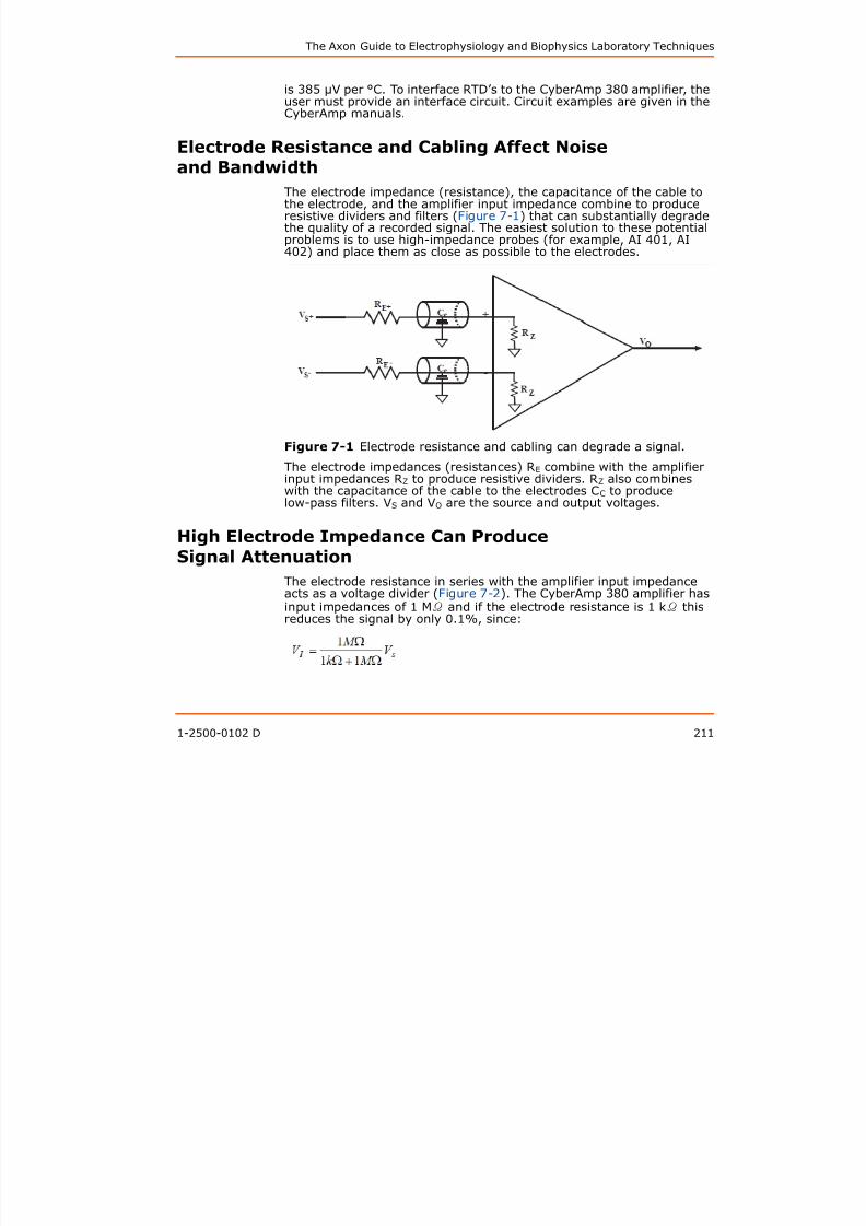
8/13/2019 User Guide v3
http://slidepdf.com/reader/full/user-guide-v3 212/302
1-2500-0102 D 211
Figure 7-1 Electrode resistance and cabling can degrade a signal.
The electrode impedances (resistances) RE combine with the amplifierinput impedances RZ to produce resistive dividers. RZ also combineswith the capacitance of the cable to the electrodes CC to producelow-pass filters. VS and VO are the source and output voltages.
High Electrode Impedance Can ProduceSignal Attenuation
The electrode resistance in series with the amplifier input impedanceacts as a voltage divider (Figure 7-2). The CyberAmp 380 amplifier hasinput impedances of 1 MΩ and if the electrode resistance is 1 kΩ this
reduces the signal by only 0.1%, since:
Transducers
However, if the electrode resistance is 100 kΩ, the signal would bereduced by about 9.1%, since:
The solution to high electrode resistance is to use a high-inputimpedance amplifier. If using a CyberAmp 380 amplifier, then youshould use a high-impedance probe between it and the electrodes. TheAI 401 x10 Low-Noise Differential amplifier probe and the AI 402 X50Ultra Low-Noise Differential amplifier probe both have inputimpedances measured in the teraohms (1012 Ω).
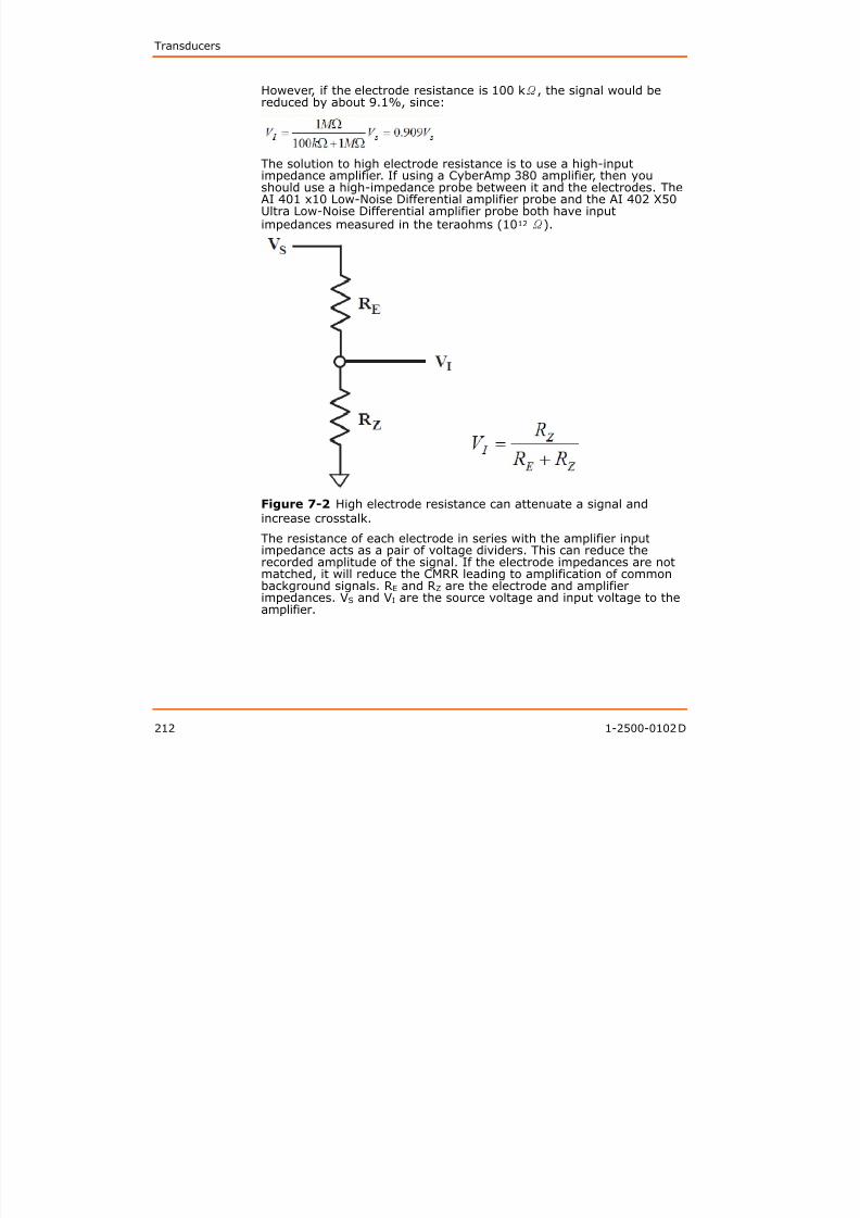
8/13/2019 User Guide v3
http://slidepdf.com/reader/full/user-guide-v3 213/302
212 1-2500-0102 D
Figure 7-2 High electrode resistance can attenuate a signal andincrease crosstalk.
The resistance of each electrode in series with the amplifier inputimpedance acts as a pair of voltage dividers. This can reduce therecorded amplitude of the signal. If the electrode impedances are notmatched, it will reduce the CMRR leading to amplification of commonbackground signals. RE and RZ are the electrode and amplifierimpedances. VS and VI are the source voltage and input voltage to theamplifier.
The Axon Guide to Electrophysiology and Biophysics Laboratory Techniques
Unmatched Electrode Impedances Increase
Background Noise and Crosstalk
When making differential measurements such as EMG, EKG and EEG itis important that both electrodes have similar properties. As we haveseen above, high electrode impedance can produce signal attenuation.
If we apply Figure 7-2 to both inputs of Figure 7-1, we see that wecould easily get greater attenuation of the signal at one electrode thanat the other. This can substantially degrade the common mode rejectionratio (CMRR) and result in amplification of common background signalsthat would otherwise be rejected.
For a differential amplifier, the CMRR is the ratio of the response for asignal at just one input to the response for a common mode signal(applied to both inputs) of the same amplitude. The CMRR of theCyberAmp 380 amplifier is 100 dB (at high gain). That is, the output
voltage with a signal applied to just one input is 100,000 times greaterthan the output voltage with the same signal applied to both inputs.(The ratio of amplitudes is measured in decibels wheredB = 20 log10(Vout /Vin). A ten-fold increase in the ratio equals a 20 dBincrease (see Chapter 6: Signal Conditioning and Signal Conditionerson page 179).
If the electrode impedance of one electrode connected to a CyberAmp380 amplifier is 1 kΩ and that of the other electrode 10 kΩ then theCMRR of the system as a whole is reduced 1,000 fold to 41 dB.
Applied to a single channel of the CyberAmp 380 amplifier:

8/13/2019 User Guide v3
http://slidepdf.com/reader/full/user-guide-v3 214/302
1-2500-0102 D 213
The difference equals 0.009:
As for the problem of the signal attenuation, the solution to a mismatchof electrode resistances is to use an amplifier probe with very highinput resistance such as the AI 401 and the AI 402 probes. With each ofthese probes, the electrode impedances used in the example are toosmall to have any influence on the CMRR of the probes.
If high-input impedance probes are not available, the CyberAmp 380amplifier has a built-in capacity to measure electrode impedances andthis should be carried out prior to each recording session to ensure a

8/13/2019 User Guide v3
http://slidepdf.com/reader/full/user-guide-v3 215/302

8/13/2019 User Guide v3
http://slidepdf.com/reader/full/user-guide-v3 216/302
Transducers
EKG
There are probably more books available on electrocardiogram (EKG)recording and analysis than any other electrophysiological topic. Thesignals are usually of large amplitudes and readily recorded without theneed for any amplifier probes. As electrode spacing is reduced, there isan increasing possibility of recording unwanted EMG signals from
neighboring muscles. Consequently, the traditional electrode sites areworth considering. The AI 417 passive 2 mm adapter provides a singledifferential EKG channel and plugs directly into the CyberAmp 380amplifier.
The normal frequency range of the mammalian EKG is 0.2–100 Hz; itsamplitude size is up to 2–3 mV.
EEG
The electroencephalogram (EEG) ranges from 10–300 μV in amplitudeand has a frequency range from 0.2–50 Hz. A single differential EEGchannel is best recorded with the assistance of one of the low-noise AI400 series active probes.
Nerve Cuffs
Nerve-cuff recordings have a frequency response to 10 kHz and anamplitude in the low microvolt range. The AI 402, x50 Ultra Low-NoiseDifferential amplifier probe is designed for this application, with 10 kHz
noise of less than 0.18 μVrms (1.1 μVp-p) in the 0.1–10 kHz bandwidth.The nerve cuffs themselves are very simple to make by running bare
8/13/2019 User Guide v3
http://slidepdf.com/reader/full/user-guide-v3 217/302
216 1-2500-0102 D
y p y gstainless steel fine wires through a small length of silicone tubing splitlongitudinally. Any bared wires that are in contact with the outersurface of the cuff can be insulated with silicone adhesive.
Metal Microelectrodes
The impedance of metal microelectrodes may be several hundredkilohms or more. All of the low-noise AI 400 series active probes aresuitable for recording from high-resistance microelectrodes. Since theinput capacitance of the AI 401 differential amplifier probe isapproximately 5 pF, the largest electrode resistance consistent withmaintaining a 10 kHz bandwidth is about 3 MΩ.
The Axon Guide to Electrophysiology and Biophysics Laboratory Techniques
Bridge Design for Pressure and Force Measurements
Pressure and force transducers are often constructed using straingauges connected in a Wheatstone bridge circuit. The basic circuit isshown in Figure 7-3.
The Wheatstone bridge should be considered as two pairs of resistive
dividers with the output voltage equaling the difference between thevoltages at (A) and (B). The bridge circuit is good for detecting smallchanges in resistance, and the output is linear in the region of balance,for example, when the voltage difference is small.

8/13/2019 User Guide v3
http://slidepdf.com/reader/full/user-guide-v3 218/302
1-2500-0102 D 217
Figure 7-3 Wheatstone Bridge circuit with amplifier.
The largest output comes from having strain gauges for all fourresistive elements, although physical constraints may require the userto have only two or even one “active” element. For applications whereonly two gauges can be used, they should be placed in positions R1 andR2 and the gauges should be located such that one increases inresistance and the other decreases in resistance during the appliedpressure or force. This is usually achieved by placing the elements onopposites sides of the beam under strain. When choosing strain gauges,keep in mind that semiconductor types have outputs ten times higherthan metal-film types.
Transducers
The sensitivity of a bridge circuit decreases with increasing temperatureand some applications may therefore require the addition of atemperature compensation circuit that should be placed as close aspossible to the bridge in order to experience the same temperaturechanges.
Pressure MeasurementsIn the past, high-quality pressure transducers were very expensive andsuffered from significant temperature sensitivity. The introduction ofsemiconductor pressure transducers has greatly reduced the cost,decreased the temperature sensitivity and enhanced the range oftransducer devices available.
An important point when measuring very low pressures is to set theheight of the pressure transducer to that of the sense location in order
to avoid hydrostatic errors introduced by fluid-filled catheters. Pressuretransducers should also be kept out of the range of heat sources suchas heat lamps to avoid temperature-induced increases in the signaloutput.
Major producers of semiconductor pressure sensors include Honeywell,Inc. (Minneapolis, MN). Blood pressure transducers from CobeLaboratories, Inc. (Lakewood, CO) have a usable range of -50 to+ 300 mmHg. All pressure transducers can be interfaced to the AxonCyberAmp 380 amplifier via the AI 490 Connector and AI 491 Cable
Kits.
Force Measurements

8/13/2019 User Guide v3
http://slidepdf.com/reader/full/user-guide-v3 219/302
218 1-2500-0102 D
Force Measurements
The requirements for force measurements are so diverse that manypeople need to make their own force transducer, although some arecommercially available (for example, Grass Instruments Company,Quincy, MA). Force transducers have some compliance and you mustconsider this when choosing transducers. For example, with the Grass
Instruments FT10, a force of 100 N will stretch the device by 1 mm.For user-designed force transducers, the two main choices are betweenresistive or semiconductor strain gauges. Resistive gauges are cheaperand generally more rugged while semiconductor strain gauges aresmaller and about 10 times more sensitive. Strain gauges are availablefrom Measurement Specialties, Inc. (Hampton, VA).
User-designed force transducers can be interfaced to the CyberAmp380 amplifier via the AI 490 Connector and AI 491 Cable Kits.
The Axon Guide to Electrophysiology and Biophysics Laboratory Techniques
Acceleration Measurements
Accelerometers can consist of piezoelectric pressure sensors attachedto a test mass, small enough for physiological experiments.Piezoelectric accelerometers can have a wide frequency range (1 Hz to25 kHz) and a wide dynamic range (0.01–2,500 g). Accelerometers canalso consist of strain gauges attached to a mass. Alternative systems
use feedback to prevent the test mass from being displaced; theamount of the applied feedback force represents the output signal.
Length Measurements
Implantable Length Gauges
Length can be measured inside an animal using mercury-filled or
saline-filled silicone tubing length gauges (Lemon and Prochazka,1984). As the tubing is stretched, the impedance of the transducerincreases. To avoid the generation of bubbles in the tubing, ahigh-frequency AC signal is used with an AC bridge circuit. In practice,these gauges have many difficulties and may not be much better thancinematography techniques using markers on the limb joints formeasuring muscle lengths.
Linear Potentiometers
Linear potentiometers are inexpensive and very simple to use but mustbe perfectly aligned to avoid internal damage. Linear potentiometerscan be interfaced to the Cyber-Amp 380 amplifier via the AI 490

8/13/2019 User Guide v3
http://slidepdf.com/reader/full/user-guide-v3 220/302
1-2500-0102 D 219
can be interfaced to the Cyber-Amp 380 amplifier via the AI 490Connector and AI 491 Cable Kits.
Linear Variable Differential Transformers (Lvdt)
Linear variable differential transformers are used for accurate andstable measurement of linear position and displacement. Rotary
variable differential transformers (RVDT) are similarly used to measurerotation. These devices are very rugged and since there is no contactbetween the core and the body of the LVDT (or RVDT), there is nofriction or wear, providing essentially infinite life. Linearity of ±0.25%over the full range is typical (ADS Transicoil, Inc., Collegeville, PA).
Self-Heating Measurements
As a result of applying an excitation current or voltage to thetemperature measurement sensor, power is dissipated in the sensor.This power dissipation causes the temperature of the sensor to riseabove the ambient temperature that is being measured. Thisphenomenon is referred to as “self heating.” For most of thetemperature sensors used in physiology, it is necessary to keep the
Transducers
power dissipation to a few milliwatts or less. If this condition is met,temperature changes of less than 0.01°C can be measured.
Other transducers, such as strain gauges, are temperature-sensitive;therefore it is important not to allow self heating in these transducersto cause a temperature rise sufficient to affect the measurement.
Isolation MeasurementsIn industrial environments, it is common for signal leads fromtransducers to be run over long distances past machinery that caninduce large voltages in the leads. To protect the measurementinstrument, isolation amplifiers should be used for each transducer.Induced voltages are not commonly a problem in animal physiologyapplications and, therefore, isolation is not required. Note that ifmeasurements are to be made from human subjects, isolated probes
that are approved for human use must be used.
Insulation Techniques
Electrodes that are implanted for long-term recording eventually faileither due to the rupture of a solder joint, breakage of wires at pointsof repeated flexion, or moisture penetration through the insulation.Although teflon-insulated wire is commonly used, when it is connectedto the leads of the transducer it is difficult to join the teflon insulation to
the insulation on the transducer leads. A solution is to etch the teflon sothat it will adhere to the adhesive used to join the two insulations. Inpractice it is often faster and better to use PVC-insulated wires because
8/13/2019 User Guide v3
http://slidepdf.com/reader/full/user-guide-v3 221/302
220 1-2500-0102 D
practice it is often faster and better to use PVC insulated wires becauseit is much easier to make a strong adhesion, even though PVC is morepermeable to water over the long term. Also, Araldite AV138M(CIBAGEIGY) and Epoxylite #6001 (Epoxylite Corporation, Anaheim,CA) both provide excellent water-resistant insulation for rigidapplications.
Special attention should be paid to providing strain relief where wires,and particularly connections, are repeatedly flexed. Sliding a length ofsilicon tubing over the stress region often reduces this problem.
Further Reading
Cain, C., Welch, A. J., Thin-film temperature sensors for biologicalmeasurement. IEEE Trans. Biomed. Eng. BME-21(5), 421–423, 1974.
Cooke, I.R., Brodecky, V., Becker, P.J., Easily implantable electrodes for
chronic recording of electromyogram activity in small fetuses. J.Neurosci. Meth. 33, 51–54, 1990.
Geddes, L. A., Baker, L. E., Principles of Applied BiomedicalInstrumentation. John Wiley & Sons, New York, 1989.
The Axon Guide to Electrophysiology and Biophysics Laboratory Techniques
Horowitz, P., Hill, W., Measurements and signal processing. The Art ofElectronics, 14. Cambridge University Press, Cambridge, 1986.
Lemon, R., Prochazka, A. Eds. Methods for neuronal recording inconscious animals. IBRO Handbook Series: Methods in theNeurosciences, Vol. 4. John Wiley & Sons, Chichester, 1984.
Loeb, G. E., Gans, C., Electromyography for Experimentalists.
University of Chicago Press, Chicago, 1986.
8/13/2019 User Guide v3
http://slidepdf.com/reader/full/user-guide-v3 222/302
1-2500-0102 D 221
Transducers

8/13/2019 User Guide v3
http://slidepdf.com/reader/full/user-guide-v3 223/302
222 1-2500-0102 D
8Laboratory Computer Issues andConsiderations
Chapter 8 provides an overview of personal computers. The earliersections give more detailed information on computer options and the
issue of price vs. performance. The last section provides a glossary ofcomputer terms that you may come across when researchingcomputers.
Select the Software First
The first consideration when setting up a personal computer is todetermine which software packages will be used, and what kind of
computer that software will run on. For specialized applications, such asscientific analysis packages, it is not safe to assume that comparablepackages are available for both Macintosh and Windows computers. Ifone needs a software package for the acquisition and analysis ofmicroelectrode voltage-clamp and current-clamp data, the AxonpCLAMP® software suite is available for Windows.
How Much Computer do you Need?
The Machine Spectrum: Capability vs. Price
Once you have determined the type of computer you are going to buy,

8/13/2019 User Guide v3
http://slidepdf.com/reader/full/user-guide-v3 224/302
1-2500-0102 D 223
y yp p y g g y,you need to decide how much you are willing to spend for performanceand convenience. The main components of the computer that you needto consider are discussed in the following sections. Although verypowerful computers have become relatively cheap in recent years, it isstill worth considering the motivations for upgrading the various systemcomponents.
Memory
RAM (Random Access Memory) is the physical device used to storeprograms and data while the computer is running. When the computerpower is off, RAM cannot hold any information, so it is referred to as “volatile” memory. It is used because instructions and data can be readfrom, and written to, RAM much faster than any other type of memorydevice. How much RAM you need and can use depends on the type ofcomputer you buy as well as the capabilities of the programs you use.
The usefulness of extra memory depends on the type of applicationsthat you will be running. Acquiring and analyzing very large datasets ingeneral requires more memory than acquiring and analyzing smalleramounts of data.
Laboratory Computer Issues and Considerations
Hard Drive
At the time of writing, 500 GB hard drives are not uncommon, and harddrives with capacity of a terabyte or more are now widely available toconsumers.
For traditional electrophysiology experiments, these hard drives providemore than enough storage. For applications that include live cell video
at high frame rates, a terabyte of storage is not enough for long-termarchiving of data. The good news is that hard drives using USB,Firewire, or SATA can be stacked externally, and are cheap enough tobe able to keep up with the increasing amounts of data.
For data acquisition, hard disk drive performance may be important. Torecord long segments of unbroken data, direct acquisition to disk(rather than memory) is necessary, and the speed of acquisition islimited by the drive performance. High hard drive speeds of 5,400 RPMare standard, and for a small price premium 7,200 RPM drives are
readily available.
Graphics Card
Recent versions of the Windows and Macintosh operating systems havenumerous extraneous “eye candy” features that can consume a largeproportion of a system’s resources without any tangible benefit. To freeup the main system processor, dedicated high-powered graphicsprocessors are now included in most modern computer systems.
Computations required to render high-speed or 3D graphics areperformed on the graphics card, freeing up the system processor forother tasks. The purchase of a high-end graphics card can thereforeincrease overall system performance.

8/13/2019 User Guide v3
http://slidepdf.com/reader/full/user-guide-v3 225/302
224 1-2500-0102 D
c ease o e a syste pe o a ce
Peripherals and Options
One of the design principles of personal computers has been themodularity of design to accommodate user-specific functionality. The
descriptions below discuss the peripherals most pertinent to laboratorysetups.
Data Backup
As common and everyday as personal computers have become, harddisks are complex mechanical devices requiring precise tolerances intheir operation, and are subject to mechanical failure. The lifetime ofhard disks is usually several years, but manufacturing defects, physical
shocks, or too many power-on cycles can make your hard disk ready tofail at any moment. It is essential that a disk full of programs and databe backed up regularly.
There are two common methods of backing up data: you can backup toanother hard drive, or back up to an optical medium such as CD or
The Axon Guide to Electrophysiology and Biophysics Laboratory Techniques
DVD. With the advent of rewritable optical disk drives, it is possible tostore 680 MB of data on a CD, and 4.4 GB on a single-layer DVD.
Although outstripped by hard drives for storage capacity, opticalstorage has the advantage of being compact for small amounts of dataand electrically stable. Another clear advantage of optical storage isthat once a CD/DVD has been closed, there is a very low chance ofoverwriting data. With a hard drive, there is a much higher chance of
losing data through accidental overwrite unless special precautions aretaken.
On the other hand, hard drives allow data to be recovered andreorganized relatively easily. Optical disks can be almost impossible torecover once they become scratched, and reorganizing data requiresdata transfer and re-burning.
Recommended Computer Configurations
Because computer state-of-the-art changes so quickly, please consultthe Molecular Devices web site for the latest recommended computerspecifications.
Glossary
A/D converter
An Analog-to-Digital converter (ADC) maps analog measurements todigital numbers that the computer can store and use in calculations.See Analog and Digital.

8/13/2019 User Guide v3
http://slidepdf.com/reader/full/user-guide-v3 226/302
1-2500-0102 D 225
g g
Analog
Real signals in the physical world are described as analog, meaning thatthe values change in a continuous manner. A mercury thermometer isan analog measurement device; the mercury rises smoothly in
response to changing temperature. However, the computer requiresdiscrete digital numbers to describe measurements of the data. SeeA/D converter and Digital.
ASCII
American Standard Code for Information Interchange. A standardized7-bit code for exchanging information between computer systems. The128-character set consists of the alpha-numeric and punctuation
characters, as well as control codes such as Escape and CarriageReturn. Files on a computer are often stored in a simple ASCII format,so that they can be easily transferred and read by different systemsand programs.

8/13/2019 User Guide v3
http://slidepdf.com/reader/full/user-guide-v3 227/302
The Axon Guide to Electrophysiology and Biophysics Laboratory Techniques
Device driver
Software that acts as an extension to the operating system, usually forsupporting a hardware device. Mouse pointing devices and networkcards are common devices that require a device driver to be loadedwhen booting the system up. On PC computers, device drivers are filesthat traditionally have a .SYS filename extension.
Digital
Data represented in discrete, discontinuous form is digital, as opposedto the smooth representation of data as measured by an analog device,such as a pen chart recorder. Computers require discrete digitalnumbers for storage and processing. See A/D converter and Analog.
DPI
Dots Per Inch is a measure of resolution on a printed page or computerscreen. The more dots per inch, the sharper that text or a graphicimage will appear. A laser printer typically has a resolution of 300 DPI.
EEPROM
Electrically Erasable Programmable Read-Only Memory. Allows ROMmemory chips to be reprogrammed with new information by users inthe field. See ROM.
I/O Interfaces
An I/O interface defines the physical interface and communicationmethod for devices attached to the computer, such as the display,
8/13/2019 User Guide v3
http://slidepdf.com/reader/full/user-guide-v3 228/302
1-2500-0102 D 227
et od o de ces attac ed to t e co pute , suc as t e d sp ay,printer, mouse and disk storage device. For devices attached internally,such as the display adapter, the physical I/O interface is the computer’sinternal bus. For external devices, for example, the mouse or printer,there are several interfaces implemented on Windows and Macintoshcomputers.
PARALLEL PORT
The parallel port interface, which exists primarily in the Windows world,allows eight bits of data to be transferred at a time (“in parallel”). Itoffers high speed, but its design allows mostly one-waycommunication; the external device is very limited in the signals it cansend back to the computer. As a result the only devices designed to usethe parallel port are those that mostly receive data, the most commonexample being the printer. While most consumer computers implement
this port as a 25-pin connector, commercial printers often use a 36-pinCentronics connector.
Parallel ports are becoming uncommon with the advent of USB printers.

8/13/2019 User Guide v3
http://slidepdf.com/reader/full/user-guide-v3 229/302
The Axon Guide to Electrophysiology and Biophysics Laboratory Techniques
Microprocessor
A microprocessor is a single integrated circuit chip that combinesfunctions for doing logical and mathematical operations, managingmemory and communicating with external devices. It is the maincontrol center of a microcomputer.
Operating systemAn operating system manages the hardware in a computer andprovides a set of services for an application program, such as writingdata to a disk drive.
Parallel port
A type of communication interface that transfers data across severalparallel lines. Communication is mostly one-way, and the length of the
connecting cable is limited. In the PC, the parallel port is used mainlyfor connecting printers.
PC
Originally referred to the IBM PC, but now refers to any computercompatible with the IBM PC designs based upon Intel CPUs.
RAM
Random Access Memory is composed of specialized integrated circuitsdesigned for storing programs and data. RAM can be quickly read fromand written to, so programs execute quickly.
However, when the computer power is off, RAM cannot hold any

8/13/2019 User Guide v3
http://slidepdf.com/reader/full/user-guide-v3 230/302
1-2500-0102 D 229
However, when the computer power is off, RAM cannot hold anyinformation.
Resolution
The “sharpness” of images and characters on the computer screen or
on printer output. Most accurately described in units of dots per inch.
ROM
Read Only Memory resides on integrated circuits that hold informationwhich is not lost when power is turned off. The contents of the ROM areusually loaded by the manufacturer and are not alterable by the user.
RS-232
A common, standard protocol for communicating over serial ports. It isa general two-way communication interface that transmits data on asingle line and receives data on a single line.
Laboratory Computer Issues and Considerations
SCSI
Small Computer System Interface. This is a type of parallel interfacethat provides for higher speeds than were possible in the older serial orparallel interfaces, while allowing multiple devices to be connected to asingle port.
Serial portA legacy standard connection, which provides a general two-waycommunication interface that transmits data on a single line andreceives data on a single line. The serial interface no longer exists inmost types of computers. Also known as a RS-232 serial port.
Throughput
A measure of performance describing how much data per unit of time
can be transferred from device to device in a computer system.
Video display card
A specialize circuit card to handle the complexity of graphics display.High-end graphics cards can be added to computers to upgrade theirstandard display speeds, resolution, and number of colors.

8/13/2019 User Guide v3
http://slidepdf.com/reader/full/user-guide-v3 231/302
230 1-2500-0102 D

8/13/2019 User Guide v3
http://slidepdf.com/reader/full/user-guide-v3 232/302
Acquisition Hardware
12:00 PM 17
12:30 PM 18
1:00 PM 19
1:30 PM 19
2:00 PM 19
2:30 PM 18
3:00 PM 16
3:30 PM 15
Table 9-1 Example Temperature Data.
Time Digitized Temperature °C

8/13/2019 User Guide v3
http://slidepdf.com/reader/full/user-guide-v3 233/302
232 1-2500-0102 D
Figure 9-1 Analog-to-digital conversion.
This figure illustrates the analog and the digital representations of thetemperature data presented in Table 9-1.
A much easier way to accomplish the same task would be to use a dataacquisition board in the computer to directly record the temperatureevery 30 minutes. In this case the thermometer must report thetemperature in a form that the analog-to-digital converter (ADC) canread. Nearly all ADCs require that the data be presented as a voltage.To do so, one uses a different type of thermometer, such as atemperature-dependent resistor in an appropriate circuit, thatgenerates an analog voltage proportional to the analog temperature.The computer is instructed to initiate an analog-to-digital conversionevery 30 minutes and store the results on disk.
Sometimes the computer is required to generate an analog waveformthat will be proportional to a list of numbers that are held in memory oron disk. In this case, a digital-to-analog (D/A) converter (DAC) is used.
The Axon Guide to Electrophysiology and Biophysics Laboratory Techniques
The principles of operation of a DAC are similar to those of an ADC, butthe operation is the reverse.
Quantization Error
The ADC converter generates binary numbers that have finiteresolution. That is, a small range of analog values will all produce thesame binary number after conversion. Returning to thetemperature-measurement example above, the hypothetical ADCrounded off all of the temperature values to the nearest degree Celsiusreading. That is, only numbers between 0 and 99°C in steps of 1°Cwere allowed. Clearly, the temperature changes continuously betweeneach 30-minutes reading, not in 1 °C jumps. The range of analogvalues that are recorded as the same digital number is the quantizationerror.
In an ADC, the total measurement range (for example, 0–100°C) isdivided into a fixed number of possible values. The number of values isa power of two, often referred to as the number of “bits.” Commonly,these values are:
8 bit = 28 = 256 values
12 bit = 212 = 4,096 values
16 bit = 216 = 65,536 values
To illustrate the impact on the resolution of using an 8-bit, 12-bit or16-bit ADC, consider the temperature-measurement example wherethe electronic thermometer circuit generates an analog outputfrom-10 V to +10 V for temperatures in the range -100°C to +100°C.In this case, the resolutions are:
8 bit = 78.4 mV = 0.784°C

8/13/2019 User Guide v3
http://slidepdf.com/reader/full/user-guide-v3 234/302
1-2500-0102 D 233
12 bit = 4.88 mV = 0.0488°C
16 bit = 0.305 mV = 0.00305°C
If the ADC is preceded by a programmable-gain amplifier, signals that
occupy only a small range, for example, ±1 V, can be amplified beforeconversion so that the full resolution of the ADC can be utilized.
The resolution of a 12-bit ADC with an input range of ±10 V is 4.88 mV.Although this resolution does not represent a difficult number for acomputer-based system to use, some researchers preferred a roundnumber such as 5.00 mV. This could easily be achieved by setting thespan of the ADC to ±10.24 V instead of ±10 V. Now, many ADCsystems are now designed with the ±10.24 V span (for example, theAxon Digidata® 1440A data acquisition system).
Acquisition Hardware
Choosing the Sampling Rate
There is a well-known theorem known as the sampling theorem or theNyquist theorem stating that data should be sampled at a frequencyequal to twice the bandwidth of the signal or faster in order to preventan artifactual increase in the noise, due to a phenomenon known asaliasing (see Chapter 11: Noise in Electrophysiological Measurements
on page 259), and guarantee that the analog signal can bereconstructed unambiguously from the digital samples.
In practice, it is common to sample at a rate significantly faster thanthe minimum rate specified by the sampling theorem. This is known asoversampling. Exactly how much oversampling should be used dependsupon the type of experiment.
For experiments where the data are analyzed in the frequency domain(for example, noise analysis, impedance analysis), it is common tooversample only modestly. The main concern is to prevent aliasing. An
anti-aliasing filter is introduced between the signal source and theanalog-to-digital converter to control the bandwidth of the data.
The factor of twice the analog bandwidth required by the samplingtheorem is only applicable if the anti-aliasing filter is ideal, for example,the gain is unity in the pass band and it abruptly changes to zero in thestop band. Ideal filters cannot be realized, although they can be closelyapproximated. For frequency-domain analysis it is common to usesharp cutoff filters such as Butterworth or Chebyshev realizations.Sampling is typically performed at 2.5 times the filter bandwidth. For
example, if the data are filtered at 10 kHz they should be sampled atabout 25 kHz. Slower sampling rates are unacceptable. Faster samplingrates are acceptable, but offer little advantage and increase the storageand analysis requirements.
For experiments where the data are analyzed in the time domain (for

8/13/2019 User Guide v3
http://slidepdf.com/reader/full/user-guide-v3 235/302
234 1-2500-0102 D
For experiments where the data are analyzed in the time domain (forexample, pulse analysis, I-V curves), greater oversampling is requiredbecause reconstructing the analog signal requires not only an idealanti-aliasing filter but also an ideal reconstruction filter. The simplestand most common reconstruction filter is to join each sample by a
straight line. Other techniques, such as cubic-spline interpolation, canbe used, but due to their much more demanding computationalrequirements they are used infrequently.
The reconstruction problem is discussed in the Sampling Rate section inChapter 11: Noise in Electrophysiological Measurements on page 259.There is no commonly accepted rule regarding the sampling rate ofdata for time-domain analysis. In general, five times the databandwidth is a common sampling rate, and ten times is consideredgood. Sampling at 20 times is excessive and is rarely used.
The Axon Guide to Electrophysiology and Biophysics Laboratory Techniques
Converter Buzzwords
The terms in this section are defined for a D/A converter. With simplereorganization, these definitions can be re-cast for an A/D converter.Only the more esoteric terms have been defined in this section. It isassumed that the reader already understands conventional terms suchas “voltage offset.”
Gain Accuracy
Gain accuracy is the closeness with which the output of the D/Aconverter corresponds to the specified full-scale value when the digitalinput to the D/A converter is the maximum value.
Linearity Error
Linearity error is the maximum deviation of the D/A output from a
straight line drawn between the minimum and the maximum output.
Differential Nonlinearity
When the digital control word changes by a minimal step, for example,one least-significant bit (LSB), the output value should change by 2-n ofthe full-scale value, where n is the number of bits in the converter. Anydeviation from this ideal change is called the differential nonlinearityerror. It is expressed in multiples of LSBs.
Least Significant Bit (LSB)
LSB is the value of the smallest possible digital increment.
Monotonicity

8/13/2019 User Guide v3
http://slidepdf.com/reader/full/user-guide-v3 236/302
1-2500-0102 D 235
Monotonicity
Monotonic behavior means that for every increase in the digital input tothe D/A converter there will be an increase in the analog output. Thisrequires that the differential nonlinearity error be less than 1 LSB.
Deglitched DAC Outputs
When the input to a digital-to-analog converter changes value, theanalog output ideally moves rapidly and monotonically towards its newvalue. While usually this is the case, for certain changes in value atransient is superimposed on the changing output. This transient isknown as a “glitch.”
Glitches occur when several bits in the control word change. Each bit isconnected to a set of internal digital logic and analog switches. There isvariability in the response time of each part of the circuit, and thereforethe response to the new control word does not happen at the sameinstant for each bit. In addition, charge is injected from the digital logic
Acquisition Hardware
circuitry into the analog switches. Glitches are worst when a largenumber of the bits of the digital input to the D/A are changed. Forexample, when the analog output is required to go from negative topositive, the digital input bits can change from 1111 1111 1111 to 00000000 0000. That is, every single bit changes. This change generatesthe worst glitch.
Glitches can be prevented by including a sample-and-hold circuit at the
output of the D/A converter. The sample-and-hold is normally in the “sample” mode so that the output of the D/A converter feeds straightthrough. However, for one or two microseconds, perhaps less, after thedigital input to the D/A converter is updated, “hold” mode is selected sothat the glitch, if present, is blocked.
In modern integrated-circuit D/A converters, efforts are made in thedesign of the chip to match the propagation and activation delays ofeach bit in the circuit and to minimize the charge injection so thatglitches are small in the first place. It is thus becoming increasingly less
common for a deglitching circuit to be included. On the other hand, thehigh-level of integration in modern D/A converters sometimesintroduces another problem, called feedthrough noise. This problemoccurs when the digital latches that contain the word for the D/Aconverter are integrated into the same chip. It may happen thatbecause of the proximity of the digital circuits to the D/A converter,digital noise couples into the D/A converter circuit. The coupled signalmanifests itself as a pulse on the output of the D/A converter circuiteach time the digital word is updated. Strangely, this feedthrough noiseoften appears even if the D/A value is being held constant. This isbecause, for simplicity, most software that simultaneously performsA/D and D/A conversions updates the D/A word once per A/D sample,even if the D/A value is not changing. The best solution is to eliminatethe feedthrough noise at its source by using separate integrated circuitsfor the D/A converter latches. This is the approach used in the Digidata

8/13/2019 User Guide v3
http://slidepdf.com/reader/full/user-guide-v3 237/302
236 1-2500-0102 D
/ pp g1440A digitizer.
Timers
Most ADC systems have several timers available for a multitude oftasks. The most essential is the provision of a regular clock signal toinitiate each A/D conversion. In most systems, one D/A conversion isperformed for each A/D conversion, but this is not required and somesystems provide for running the D/A converter at a different clock rateto the A/D converter.
Additional timers are used to implement “gear shifting.” This is atechnique wherein the acquisition rate is rapidly changed (gear shifted)
during acquisition from a low to a high rate or vice versa, withoutstopping the acquisition.
Uncommitted timers are generally provided for use in frequencymeasurement, event counting or interval timing. For example, the
The Axon Guide to Electrophysiology and Biophysics Laboratory Techniques
frequency of nerve spikes can be counted if they are first detected byan event detector that puts out a digital pulse for every spike. Anexample of event counting is the measurement of the number ofphotons collected by a photomultiplier tube in a fixed interval. Anexample of interval timing is measurement of the period of a spinningoptical filter wheel so that the optical data collected can be normalizedagainst fluctuations in the rotational speed of the wheel.
Digital I/O
Digital outputs are used during experiments to control externalequipment. For example, an oscilloscope can be triggered before theacquisition commences, or a flash lamp or an isolated stimulator couldbe activated during the acquisition. In other experiments, severalsolenoids can be sequentially activated before, during and after theacquisition.
Digital inputs are used routinely in industrial control applications formonitoring the state of solenoids and other apparatuses, but they arerarely used in electrophysiological experiments. The main applicationfor digital inputs in electrophysiology is for triggering acquisitions andfor indicating that a tag should be attached to the data.
Optical Isolation
Computers provide quite hostile environments for plug-in dataacquisition boards. The rapid switching activity of the digital logiccircuits causes electronic noise to radiate directly into plug-in boardsinstalled by the user and to be introduced into the ground referenceused by the plug-in boards.
Ne e theless it is s all possible to design data acq isition s stems

8/13/2019 User Guide v3
http://slidepdf.com/reader/full/user-guide-v3 238/302
1-2500-0102 D 237
Nevertheless, it is usually possible to design data acquisition systemsthat do not suffer from extraneous noise pickup. This is achieved bycareful layout and good grounding. Grounding and shielding, if appliedwith great skill and diligence, can sometimes be made to work
acceptably for the A/D converter, especially when combined withdifferential recording. However, it is very difficult to achieve acceptablenoise levels on the DAC outputs. The following approach is ofteninvoked for 16-bit systems.
First, move the A/D converter off the plug-in board in the computer to aseparate board housed in an external box. This eliminates the problemsdue to direct pickup of noise generated inside the computer housing.However, it does not eliminate the noise introduced through the systemground. The noise in the system ground can be eliminated by usingoptical isolation. In this technique, the digital signals to and from thecomputer are not connected directly. Instead, an optical coupler isinterposed in each digital line. A separate power supply is provided forthe A/D and D/A side of the optical couplers. This technique allows a
Acquisition Hardware
low-noise ground to be maintained for the A/D and D/A converters andfor the experimental setup.
Operating Under Multi-Tasking Operating Systems
Data acquisition systems are not naturally compatible withmulti-tasking operating systems. As a general rule, data acquisitionsystems are designed to use all of the resources of the computer (forexample, display and disk) and they use these resources on demand,rather than when the computer makes them available.
Interrupt handling represents an acute problem for data acquisition inmulti-tasking operating systems. Usually, when an interrupt occurs animmediate response is required. If the multi-tasking operating systemis busy updating a screen for a word processor, an immediate responsewill clearly not be forthcoming. Therefore, high performance clearlyrequires that the data acquisition task runs as the foreground
application. Another problem is that modern computers generally havelong interrupt latencies of several hundred microseconds or more. Oneway to minimize the problem of excessive interrupt latency is to ensurethat the data acquisition routine has the highest priority and, in manycases, exclusive control over the computer. Another way to minimizeexcessive interrupt latency is to provide hardware support in theacquisition system. For example, a memory-buffered data acquisitionsystem can be configured by the acquisition software and left in a “primed” state. When it “sees” an external trigger it can generate an
interrupt, then commence the acquisition before it even receives aresponse from the host.
Software Support

8/13/2019 User Guide v3
http://slidepdf.com/reader/full/user-guide-v3 239/302
238 1-2500-0102 D
Nowadays fewer researchers are writing their own data acquisition andanalysis software using low-level languages and device drivers. Mostresearchers are using one of two types of commercially availablesoftware. The first type is a rich development environment such as
MATLAB or LabVIEW. This environment allows researchers to designtheir own software without having to become experts in the low-levelcontrol of the data-acquisition hardware. The second type of software isa turn-key package, such as pCLAMP® software. These packagesprovide sophisticated acquisition and analysis, but only limited ability tocustomize them. Nevertheless, they are extremely popular becausethey perform well and are easy to learn.
When choosing hardware and software for a data acquisition system,we recommend that you choose the software first and then purchase
the hardware recommended by the software applications that you haveselected.
10Data Analysis
Chapter 10 provides guidelines to selecting certain key data acquisitionparameters, and discusses current methods used in analysis of
biological data, including fitting models to data and analyzing singleion-channel recordings. The scope of this discussion is limited to brief,practical introductions with references to more detailed discussion inthis guide and in the literature. The manuals for the various softwareprograms can be used for more specific step-by-step instructions, andthe text by Dempster (1993) is a useful collection of standardtechniques in this field.
Choosing Appropriate Acquisition Parameters
Successful analysis of a data set requires that the signals be recordedusing appropriate data acquisition parameters. Following are guidelinesto selecting several critical recording parameters.
Gain and Offset
Sufficient gain and offset should be maintained on all transducers andamplifiers during data acquisition, because data review and analysis
software can usually provide only limited amounts of additional(“software”) offset and gain. More than 10x of software gain usuallyresults in excessively jagged traces; this is because the digitized signaldoes not vary smoothly but is quantized (see Chapter 9: AcquisitionHardware on page 231), and too much amplification allows thedifference between one quantization level and the next to become

8/13/2019 User Guide v3
http://slidepdf.com/reader/full/user-guide-v3 240/302
1-2500-0102 D 239
qvisible. Software offset is limited to the full range of the analog-to-digital converter (ADC) input, which is usually equivalent to about±10 V referred to the input of the ADC. Signal resolution is bestpreserved when the signal fills this voltage range without exceeding it.
Sampling Rate
The sampling rate used should be selected considering the particularexperiment. Use of excessively high sampling rates wastes disk spaceand will increase the time required for analysis. Furthermore, a highersampling rate is usually associated with a higher filtering frequency,which in turn allows a larger amount of noise to contaminate the signal.Subsequent analysis of the data may therefore require noise reduction
using analysis-time filtering, which can be time-consuming. Guidelinesto choosing the correct sampling rate are discussed in the followingparagraphs (Colquhoun and Sigworth, 1983, and Ogden, 1987).
Data Analysis
Biological signals are most commonly analyzed in the time domain. Thismeans that the time dependence of the signals is examined, forexample, to characterize the membrane response to a voltage-clamppulse. The usual rule for time-domain signals is that each channelshould be sampled at a frequency between 5 and 10 times its databandwidth. Knowing the value of the data bandwidth is required inorder to set the filter cut-off frequency during acquisition and analysis.
For a sinusoidal waveform, the data bandwidth is the frequency of thesine itself. For most biological signals, the data bandwidth is the highestfrequency of biological information of interest present in the recordedsignal. This can be determined directly by examining a power spectrumof rapidly sampled unfiltered data, though this is rarely done.Alternatively, one can estimate the number of points per time intervalrequired to give a data record whose points can be easily “connected”by eye and calculate the sampling rate directly. The data bandwidth andfilter frequency can then be calculated from the sampling rate. Forexample, if a fast action potential (1 ms to peak) is to be recorded, 25samples on the rising phase would yield a reasonably good 40 μsresolution, requiring a sampling rate of 25 kHz and an approximatedata bandwidth of 5 kHz.
The rules are more straightforward in some special cases.Single-channel recording is discussed below. For signals withexponential relaxation phases, the sampling rate needed to estimate atime constant depends on the amount of noise present; for moderatelynoise-free data, at least 15 points should be taken per time constantover a period of 4 to 5 time constants. Many fitting routines will fail if
sampling is performed over only 3 time constants, since the waveformdoes not relax sufficiently far towards the baseline. For a sum ofmultiple exponentials, the sampling rate is determined in this way fromthe fastest phase; sampling must extend to 4 time constants of theslowest phase. If this would result in too many samples, a split clock(as in the Clampex program of the Axon pCLAMP® suite) or other
8/13/2019 User Guide v3
http://slidepdf.com/reader/full/user-guide-v3 241/302
240 1-2500-0102 D
(as in the Clampex program of the Axon pCLAMP® suite) or othermethods of slowing the acquisition rate during the acquisition, could beemployed as long as at least 15 points are taken over each timeconstant.
When a set of several channels is recorded (for example, channels 0through 3), most data acquisition systems sample the channelssequentially rather than simultaneously. This is because the systemusually has only one analog-to-digital converter circuit that must beshared among the channels in the set. For example, if four channels aresampled at 10 kHz per channel, one might expect that they would besampled simultaneously at 0 μs, 100 μs, 200 μs, etc. Instead, channel0 is sampled at 0 μs, channel 1 at 25 μs, channel 2 at 50 μs, channel 3at 75 μs, channel 0 again at 100 μs, channel 1 again at 125 μs, etc.
There is therefore a small time skew between the channels; if thiscauses difficulties in analysis or interpretation, a higher sampling ratecan be used to minimize the time skew (but this may cause problemsassociated with high sampling rates, as mentioned above).
The Axon Guide to Electrophysiology and Biophysics Laboratory Techniques
An additional consideration arises from the fact that on many dataacquisition systems, including the Digidata® 1440A digitizer from MDSAnalytical Technologies, the digital-to-analog converter (DAC) isupdated whenever the ADC is read, even if there is no change in theDAC output. This means that the DAC is updated only at the samplerate over all channels. For example, if a stimulus is a 0 to 150 mV rampand 50 samples are acquired from one channel at a sampling interval of25 μs, the DAC output will appear as a series of steps each 25 μs longfollowed by an upward jump of 150 mV/50 = 3 mV, which may be toolarge for some electrophysiological applications. Therefore, if a rapidlychanging continuous waveform is applied while acquiring slowly, theoutput waveform should be checked with an oscilloscope and, ifnecessary, the sampling interval should be increased. The computerpreview of a waveform cannot be relied upon for this purpose becauseit does not account for the effect of sampling. Note, however, that sincemost users acquire significantly more samples per sweep than 50, thisproblem will not occur except in very unusual situations.
Filtering
The signal should be filtered using an analog filter device before itarrives at the ADC. As discussed in Chapter 6: Signal Conditioning andSignal Conditioners on page 179 and in Colquhoun and Sigworth, 1983and Ogden, 1987, this is done to prevent aliasing (folding) ofhigh-frequency signal and noise components to the lower frequenciesof biological relevance.
Acquisition-time filtering of time-domain signals is usually performedusing a Bessel filter with the cut-off frequency (-3 dB point; seeChapter 6: Signal Conditioning and Signal Conditioners on page 179)set to the desired value of the data bandwidth. A 4-pole filter is usuallysufficient unless excessive higher frequency noise requires the 6- or8-pole version. The Bessel filter minimizes both the overshoot (ringing)
d th d d f l f Th l tt t

8/13/2019 User Guide v3
http://slidepdf.com/reader/full/user-guide-v3 242/302
1-2500-0102 D 241
and the dependence of response lag on frequency. The latter twoeffects are properties of the Chebyshev and Butterworth filters (seeChapter 6: Signal Conditioning and Signal Conditioners on page 179 and Chapter 11: Noise in Electrophysiological Measurements on
page 259, or Ogden, 1987), which are less appropriate for time-domainanalysis.
Filtering at Analysis Time
It is sometimes reasonable to sample data at higher rates than seemsnecessary, for example, when a greater bandwidth might be requiredduring analysis. If excessive sample rates are used, the filter frequency
must be set to a higher value. Since there is more noise at higherfrequency, more noise is likely to contaminate the signal. Therefore, thedata must be filtered further during analysis in order to reduce thenoise and avoid aliasing of high-frequency signal content.
Data Analysis
This analysis-time filtering is performed using filters implemented insoftware. The Gaussian filter is most commonly used for this purposebecause of its execution speed, though the Bessel filter is employed aswell. If one wants to write a computer program for a filter, the Gaussianis easier to implement than the Bessel filter (see program example inColquhoun and Sigworth, 1983). All filters alter the waveform; forexample, a Gaussian-filtered step function deviates from the baselinebefore the time of transition of the unfiltered signal. The user canexamine data records filtered at different frequencies to make sure thatthere is no significant distortion of the quantities of interest, such astime of transition or time to peak.
Another common software filter is smoothing, the replacement of adata point by a simply weighted average of neighboring points, used toimprove the smoothness of the data in a record or graph. In contrast tothe smoothing filter, the Bessel and Gaussian types have well-knownfiltering (transfer) functions, so that (i) it is easy to specify an effectivecut-off frequency, and (ii) the effect of the filter may be compensated
for by a mathematical procedure analogous to a high-frequency boostcircuit in a voltage-clamp amplifier (Sachs, 1983). These advantagesare important if the frequency properties must be known throughoutthe analysis. If not, the smoothing filter is much faster to execute,especially on long data records, and easier to implement if one writesone’s own software.
Integrals and Derivatives
The integral function is used to calculate the area under a digitized datatrace. Applications include measuring the total charge transfer fromrecords of membrane current, and measuring the area under aminiature endplate potential. The integral is generally calculated bydirect summation of y(xi)Δxi between two cursors placed along the x
i F d t d ( ) i th lit d t ti i t d Δ

8/13/2019 User Guide v3
http://slidepdf.com/reader/full/user-guide-v3 243/302
242 1-2500-0102 D
axis. For a data record, y(xi) is the amplitude at time point xi, and Δxi is the sampling interval at that time. For a histogram, y(xi) is theamplitude of the bin at location x i, and Δxi is the bin width of bin i (this
allows for nonuniform bin width). The y values must be corrected forany superfluous baseline before integration using a fixed or slantingbaseline, as appropriate. If the sample rate were low compared to therate of change of the signal, so that y values show large changes fromone xi to the next, the integral is considerably less accurate than ifsignificantly more samples were taken. Large inaccuracies can alsooccur if the signal does not return to baseline by the end of the data setor if part of the data is corrupted by an extraneous signal. In somecases, errors in the integral can be reduced by first fitting a smoothcurve to the available data and then using the formula and parameters
of the best fit to calculate the integral.The derivative function is used to determine the rates of change of adigitized signal. This can be used to help in peak location (where thederivative will be near zero), transition detection (large positive or
The Axon Guide to Electrophysiology and Biophysics Laboratory Techniques
negative derivative), sudden departure from baseline, etc. Thederivative will, however, amplify noise, making it difficult to determinetrends. The signal should therefore be filtered beforehand or fit to afunction which can then be used to obtain a noise-free form of thederivative. However, the worse the fit, the greater the error in thederivative.
Single-Channel Analysis
Goals and Methods
The goal of single-channel current analysis is to reconstruct theidealized current waveforms from which information about themechanisms of channel function is derived. Specific information can bededuced with respect to channel state diagrams, kinetics of channelopening, closing and gating, channel barrier models, and the effects of
channel blocking agents and membrane constituent on channelfunction.
Articles that present approaches and methods used in single-channelcurrent analysis include Colquhoun and Hawkes, 1983; Colquhoun andSigworth, 1983; McManus, Blatz and Magleby, 1987; Sigworth andSine, 1987; and French et al., 1990.
The current from a single ion channel is idealized as a rectangularwaveform, with a baseline current of zero (closed-channel), anopen-channel current dependent on the conductance and membranepotential, and rapid transitions between these current levels. Inpractice, this idealized current is distorted by the limited bandwidth ofthe apparatus and contaminated by noise. Shifts in the baseline mayoccur during the recordings, and capacitative current spikes are presentin sweeps in which voltage changes are applied across the membrane.The current signal is further altered by filtering and by periodic
8/13/2019 User Guide v3
http://slidepdf.com/reader/full/user-guide-v3 244/302
1-2500-0102 D 243
The current signal is further altered by filtering and by periodicsampling. These effects can impede making confident inferences fromdata regarding channel behavior.
Sampling at Acquisition TimeIn order to adequately reconstruct the transitions, the sampling rateshould be no less than 5 times higher than the cut-off frequency of thefilter (Colquhoun and Sigworth, 1983; French et al., 1990).
Filtering at Acquisition Time
As discussed above, the input signal should be filtered with a Besselfilter during acquisition. The cut-off frequency must usually be setsufficiently low to prevent unacceptably frequent occurrences of noise,which cause false closings and false brief open-close events during theconstruction of idealized channel currents. French et al., (1990) discusshow to decide on the cut-off frequency for a particular situation: open
Data Analysis
events of longer duration are more likely to be falsely closed by noise,so it is convenient to specify the longest duration dmax that can berecorded with less than 1% occurrence of these false closings. Oncedmax has been specified, the required cut-off frequency f c can becalculated using the following combination of equations (18) and (19)in French et al., (1990):
Here FTC* is the observed rate of false threshold crossings measuredusing recordings made with an arbitrary cut-off frequency f c*. FTC* canbe measured from idealized single-channel records generated using athreshold set on the side of the baseline opposite to where transitionsare observed. This analysis can be achieved using pCLAMP software.
Analysis-Time Filtering
The digital Gaussian filter can be used for additional analysis-timefiltering of single-channel records. This introduces symmetrical timedelays at both opening and closing and can therefore be used for theunbiased estimation of latencies using the 50% criterion (Setting theThreshold for a Transition on page 244).
Generating the Events List
The first step during analysis of single-channel current records is toidealize the current records to a series of noise-free open and closedstates having infinitely short (or at least shorter than the sampleinterval) transition times. This analysis, which can be performed bypCLAMP software, results in a list of durations and amplitudes, calledthe events list. Several effects that tend to complicate thisreconstruction are briefly discussed below; more thorough discussions
8/13/2019 User Guide v3
http://slidepdf.com/reader/full/user-guide-v3 245/302
244 1-2500-0102 D
reconstruction are briefly discussed below; more thorough discussionsare presented in the cited literature.
Setting the Threshold for a Transition
A transition between states of a channel occurs when the currentamplitude passes through a threshold between two levels. The mostcommonly used threshold is 50% of the difference between the levels.The advantage of this threshold setting is that the event durations arenot biased because the values of the threshold are the same for bothopening and closing transitions.
Baseline Definition
The accuracy of the threshold method for transition detection dependson the stability of the baseline (for example, closed-channel) current or,if the baseline is unstable, on the ability of an automated procedure tocorrectly identify the baseline as it changes. A number of ways have
The Axon Guide to Electrophysiology and Biophysics Laboratory Techniques
been devised to track a moving baseline, including 1) averaging thebaseline current level to get the new baseline; 2) defining the newbaseline as that level which maximizes the number of times that thecurrent signal crosses it during the closed state (“zero crossings”method; Sachs, 1983); and 3) defining the new baseline at the peak ofthe histogram of the baseline current amplitude (for example, G.Yellen, quoted in Sachs, 1983). pCLAMP software uses a hybridapproach in which the average of the most recent closed channel
current level is averaged with the old baseline level, weighted by aselectable factor. Regardless of the method used, the user mustcarefully monitor the baseline to ensure that any automatic proceduredoes not lose track of the baseline value.
Missed Events
Events will be missed if their true durations are shorter than the deadtime of the system, which is determined by the filter cut-off frequencies
used during acquisition and analysis. Events will also be missed if theirsuperthreshold portions happen to miss the times when the signal issampled even if their durations are longer than this dead time. Theresulting error is minimal if the fastest time constant in the system ismuch longer than the sampling interval because few events will beshorter than the sampling interval. If this is not the case, the samplingrate must be increased with respect to the filter cut-off frequency (seeSection 10.4.2., “Sampling at Acquisition Time”).
False EventsThe probability of detecting false events depends on the amount andspectrum of noise in the system, the filter characteristics and the rateof sampling (French et al., 1990).
Multiple Channels

8/13/2019 User Guide v3
http://slidepdf.com/reader/full/user-guide-v3 246/302
1-2500-0102 D 245
p
The presence of multiple channels complicates the determination of thekinetic behavior of a channel. If a record shows a transition from two
open channels to one open, it cannot be determined if the transitionwas due to the closing of the first or the second channel. A number ofmethods have been proposed to deal with this ambiguity (French et al.,1990). As a precaution, the amplitude histogram of the raw data can beinspected to determine if multiple channels are present.
Analyzing the Events List
The second step in the analysis procedure is the extraction of model-specific information from the events list. Because the number of events
is usually large, it is often convenient to sort the event data into bins.The binned data may then be fit to a mathematical function whoseparameters are related to a state diagram of the channel.
Data Analysis
The most common histograms include 1) the dwell time histogram, inwhich the duration of events is binned and which can be related to statemodels; 2) the first latency histogram, in which the period of time fromstimulus onset to first opening is binned and which is used to extractkinetic information; and 3) the amplitude histogram, in which theamplitudes of the levels or of all points in the records are binned andyield information about the conductance, the system noise and theincidence of multiple channels.
Histograms
The simplest histogram is one in which a series of bins are defined,each of which has an associated upper and lower limit for the quantityof interest, for example, dwell time. Each dwell time will then fall intoone of the bins, and the count in the appropriate bin is incremented byone. In the cumulative histogram, a bin contains the number ofobservations whose values are less than or equal to the upper limit for
the bin.
Histogram Abscissa Scaling
Histograms may be scaled and displayed in a number of ways. Themost common histogram has constant bin width, a linearly scaledabscissa (x axis), and counts displayed on the ordinate (y axis). Anumber of alternatives have been developed to improve the treatmentof exponential distributions, in which low-time bins have many countsand high-time bins have few, yielding histograms that are difficult to
visualize (for example, McManus et al., 1987; Sigworth and Sine,1987). One solution is to increase the bin width logarithmically, so thatfor a single exponential, a constant number of events is expected perbin. This has the disadvantage that the presence of multiple timeconstants is not evident from the plot if the ordinate is not rescaled.These issues are discussed in the next section.

8/13/2019 User Guide v3
http://slidepdf.com/reader/full/user-guide-v3 247/302
246 1-2500-0102 D
Histogram Ordinate Scaling
If a constant bin width histogram is used, linear scaling of the ordinateis the most common (Figure 10-1 A). If a logarithmic bin width is used,several methods are common.
In one of the methods, the number of counts in each bin is divided bythe bin width and plotted on a logarithmic axis, in which case multipletime constants are evident (Figure 10-1 B). The main difficulty with thisscaling is that the bins do not have the same weight during the fitprocess (see Fitting to Histograms on page 250), because the varianceof the bin depends on the number of counts it contains. This can becompensated for using the transformation of Sigworth and Sine (1987).In this transformation the bin width is constant and the square root ofthe number of counts per bin is plotted on the ordinate, with timeplotted logarithmically on the abscissa Figure 10-1 C).
The Axon Guide to Electrophysiology and Biophysics Laboratory Techniques

8/13/2019 User Guide v3
http://slidepdf.com/reader/full/user-guide-v3 248/302
1-2500-0102 D 247
Figure 10-1 Histogram scaling.
Three representations of a dwell-time distribution with two exponentialcomponents. 5,120 random numbers were generated according to adistribution with time constants of 10 ms (70% of the events) and 100 ms(30%) and binned for display as histograms in the lower panel of each part ofthe figure. Superimposed are the theoretical probability density functions foreach component (dashed curves) and their sum (continuous curve). In eachpart of the figure the upper panel plots the absolute value of the deviation ofthe height of each bin from the theoretical curve, with dashed curves showing
the expectation value of the standard deviation for each bin. The upper panelswere plotted with vertical expansion factors of 2.1, 5.4, and 3.1 respectively.
Data Analysis
Errors Resulting from Histogramming Events Data
Problems may appear as a result of the histogram process. The firstproblem may occur in either amplitude or time histograms if the bin
size is not an integral multiple of the resolution of the signal. For adwell time, the resolution is the interval between successive samplingsof the ADC channel; for an amplitude, the resolution is determined bythe gain and the ADC. The symptom is that occasional or periodic peaksor valleys appear artifactually in the histogram. This problem is lesssevere if the bin width corresponds to many resolution intervals (forexample, 10). If bin widths are variable, the smallest bin width mustlikewise include many resolution intervals.
A second problem is called sampling promotion error. Sampling
promotion error (Sine and Steinbach, 1986) occurs because data aresampled periodically. Suppose data were acquired with 1 ms samplingrate and dwell times binned into a histogram with bin width equal to thesampling rate (1 ms) and centered around 3 ms, 4 ms, 5 ms, etc. The4 ms bin would therefore contain events whose true dwell times liebetween 3 and 5 ms (Figure 10-2). If the dwell times fall exponentiallywith increasing times, the 4 ms bin would contain more events from 3
A Linear histogram. Events are collected into bins of 1 ms width andplotted on a linear scale. The 100-ms component has a very smallamplitude in this plot.
B Log-log display with variable-width (logarithmic) binning. The numberof entries in each bin is divided by the bin width to obtain a probabilitydensity in events/s which is plotted on the ordinate.
C Square-root ordinate display of a logarithmic histogram. Note that thescatter about the theoretical curve is constant throughout the display(reproduced with permission from Sigworth and Sine, 1987).
Figure 10-1 Histogram scaling. (cont’d)

8/13/2019 User Guide v3
http://slidepdf.com/reader/full/user-guide-v3 249/302
248 1-2500-0102 D
with increasing times, the 4 ms bin would contain more events from 3to 4 ms than from 4 to 5. The subsequent fit would treat all theseevents as if they had occurred at 4 ms (the midpoint), thereby resulting
in an error. In a single exponential fit, this affects only the intercept andnot the time constant; but there may be more subtle effects in amulti-exponential fit. The error is small when the bin width is muchsmaller (perhaps by a factor of 5) than the fastest time constantpresent.

8/13/2019 User Guide v3
http://slidepdf.com/reader/full/user-guide-v3 250/302
Data Analysis
Lastly, as discussed in the section on missed events, short events maynot be detected by the 50% threshold criterion. This can give rise to anumber of errors in the extracted fit parameters, which relatespecifically to state models. For further details, consult the referencescited in French et al., 1990.
Amplitude Histogram
Amplitude histograms can be used to define the conductances of statesof single channels. Two kinds of amplitude histograms are common:point histograms and level histograms. The former use all the acquireddata points; they are useful mainly for examining how “well-behaved”is a data set. Abnormally wide distributions may result from high noiseif the signal were over-filtered, or if baseline drift had been significant.Similarly, the number of peaks will indicate the presence of multiplechannels or subconductance states. The all-points histogram willprobably not be useful for determining the conductances unless
baseline drift is small. Level histograms use only the mean baseline-corrected amplitudes associated with each event in the events list.Such histograms can be fitted to the sum of one or more Gaussianfunctions in order to estimate conductances.
Fitting to Histograms
Amplitude and dwell time histograms can be fitted by appropriatefunctions, usually sums of several Gaussian functions for the formerand sums of exponentials for the latter (see The Chi-Square Function
(Least-Squares Method) on page 253). The time constants andamplitudes can be related to the parameters of several single-channelmodels, but this will not be described here. Histogram bins containingzero counts should usually be excluded from a fit because the chi-square function (see below) is not defined when a bin i contains Ni = 0counts and therefore has σi = 0. Alternatively, adjacent bins can becombined to yield a nonzero content.

8/13/2019 User Guide v3
http://slidepdf.com/reader/full/user-guide-v3 251/302
250 1-2500-0102 D
FittingReasons for Fitting
Fitting a function to a set of data points, such as a histogram or a timeseries, may be done for any of the following reasons:
1. A function could be fitted to a data set in order to describe itsshape or behavior, without ascribing any “biophysical” meaningto the function or its parameters. This is done when a smooth
curve is useful to guide the eye through the data or if a functionis required to find the behavior of some data in the presence ofnoise.
The Axon Guide to Electrophysiology and Biophysics Laboratory Techniques
2. A theoretical function may be known to describe the data, suchas a probability density function consisting of an exponential,and the fit is made only to extract the parameters, (for example,a time constant). Estimates of the confidence limits on thederived time constant may be needed in order to compare datasets.
3. One or more hypothetical functions might be tested with respectto the data, for example, to decide how well the data werefollowed by the best fit function.
The fitting procedure begins by choosing a suitable function to describethe data. This function has a number of free parameters whose valuesare chosen in order to optimize the fit between the function and thedata points. The set of parameters that gives the best fit is said todescribe the data, as long as the final fit function adequately describesthe behavior of the data. Fitting is best performed by softwareprograms; the software follows an iterative procedure to successivelyrefine the parameter estimates until no further improvement is foundand the procedure is terminated. Feedback about the quality of the fitallows the model or initial parameter estimates to be adjusted manuallybefore restarting the iterative procedure. Fitting by pure manualadjustment of the parameters (the so-called “chi by eye”) may beeffective in simple cases but is usually difficult and untrustworthy inmore complex situations.
The two following topics will be briefly discussed below: statistics, i.e.,how good is the fit and how confident is the knowledge of theparameters, and optimization, for example, how to find the best fitparameters. The statistical aspects are well discussed in Eadie et al.,(1971); Colquhoun and Sigworth (1983) provide examples relevant tothe electrophysiologist. A number of aspects of optimization arepresented in Press et al., (1988).
Statistical Aspects of Fitting
d l h h b b l f f b b l

8/13/2019 User Guide v3
http://slidepdf.com/reader/full/user-guide-v3 252/302
1-2500-0102 D 251
Statistics deals with the probability of occurrence of events. Probabilityis difficult to define; there are two ways in which the word is used:
1. Direct probability: If we observe that N 1 of N single-channelevents have open channel durations between 10 and 20 ms, wesay that the probability p1 of this occurring is N 1 /N , as long as Nis very large. The probability density function (pdf) is analgebraic expression that when summed or integrated between10 and 20 ms gives the value of p1.
2. Inverse probability: If you are told by your physician that youhave one of three possible diseases D1, D2, or D3, and you askwhat the probability is that you have D2, the physician might
say, “It’s either 0 or 1,” meaning that either you already have D2 or you do not have it, but the physician cannot yet determinewhich of these two situations exists. To be helpful, yourphysician might give an inverse probability of 0.6, meaning that
Data Analysis
if you had D2, the probability that your particular set ofsymptoms would have been observed is 0.6.
The Likelihood Function
Inverse probability is more appropriate for the scientist who may haveN measurements of open channel durations and wants to know whichtime constant best describes their exponential distribution. For a
particular time constant, τ1, one can calculate the direct probability ofgetting those N observed durations by first calculating the probability ofobserving each duration and then multiplying these individualprobabilities together. The resulting number is called the likelihood ofthe time constant τ1. One could calculate the likelihoods for many suchvalues of τ and plot the logarithm of these likelihoods versus theirrespective τ values (Figure 10-3). If N is sufficiently large, this curvewill usually be Gaussian. The value τ* at the peak of the function iscalled the maximum likelihood value of τ. The root-mean-square
spread of the function about τ is known as the standard deviation ofτ*, though this is not the same as a standard deviation of a set ofnumbers in the direct probability case.
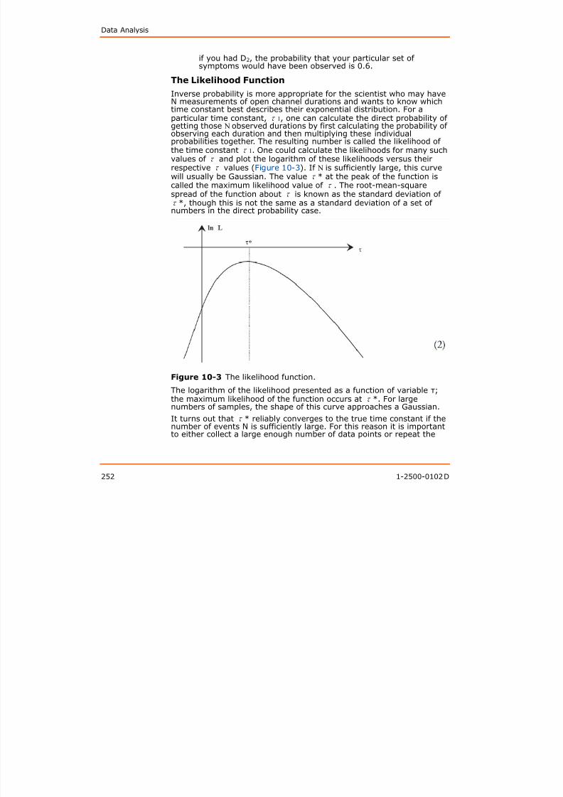
8/13/2019 User Guide v3
http://slidepdf.com/reader/full/user-guide-v3 253/302
252 1-2500-0102 D
Figure 10-3 The likelihood function.
The logarithm of the likelihood presented as a function of variable τ;the maximum likelihood of the function occurs at τ*. For largenumbers of samples, the shape of this curve approaches a Gaussian.
It turns out that τ* reliably converges to the true time constant if thenumber of events N is sufficiently large. For this reason it is importantto either collect a large enough number of data points or repeat the
The Axon Guide to Electrophysiology and Biophysics Laboratory Techniques
experiment several times so as to reduce the variation of theparameters obtained over the data sets to an acceptable level. If thenoise is large or there are sources of significant variability in the signal,the data may be useless except in a qualitative way because of largevariations of the best fit parameters between the runs. If one long runis taken instead of several smaller ones, the run can be broken up intosegments and the analysis results of the segments compared with eachother to assure that convergence is near.
Although the maximum likelihood method is the most reliable, the timerequested for the calculations may be prohibitively long. The chi-squaremethod, described below, is an alternative that requires less time.
The Chi-Square Function (Least-Squares Method)
Suppose that a set of p measurements are made at the times x1, x2, ...,xp, and that the values measured are y1, ..., yp. If each yi is measuredwith a measurement error distributed as a Gaussian with standard
deviation σ1, ..., σp, the maximum likelihood method is equivalent tominimizing the chi-square function:
where y*i is the fit value corresponding to yi. Minimizing chi-square isalso called the least-squares method. If the fit is made to a data sweep,each yi is the value measured at the time xi, and each σi is the
standard deviation or uncertainty of that value. In the typical casewhen all the σi’s are equal (for example, the uncertainty in the datadoes not depend on the time), the σiʼs can be ignored while performingthe search for the best fit parameters, but must be specified if thegoodness of fit is to be calculated. If the fit is made to a histogram,each yi is the numbers of events Ni in bin i, and each σi is √ Ni.
It is much easier to maximize the chi square function than to minimize

8/13/2019 User Guide v3
http://slidepdf.com/reader/full/user-guide-v3 254/302
1-2500-0102 D 253
It is much easier to maximize the chi-square function than to minimizethe likelihood function, whether for data or for many mathematical
functions used as models.Since the use of the chi-square function is equivalent to the use of thelikelihood function only if the uncertainties in the data (for example,noise) are distributed as Gaussians, the correctness of a least-squaresfit can depend on the characteristics of this uncertainty.
The Goodness of Fit
After a best fit has been obtained, the user might wish to know if the fitwas good. If the fit to p data points employed M free parameters, the
probability of obtaining a chi-square value greater than that of the bestfit, given p–M degrees of freedom, can be read from a table ofprobabilities of chi-square and compared to a chosen significance level.
Data Analysis
Often several models are fitted to a single set of data so as to definethe best-fit model. Horn (1987) discussed choosing between certaintypes of models using their respective chi-square values (with the Ftest) or the logarithm of the ratio of the likelihoods, which follows thechi-square distribution. These tests can help decide whether the modelcontains irrelevant parameters, for example, if a three-exponentialfunction was fitted to a set of data containing only two exponentials.
Confidence Limits for the ParametersAn estimate of the confidence limits for each of the parameters is oftenuseful. For a model with one parameter a, some fit programs will derivethe standard deviation σ from the dependence of the likelihood orchi-square on the parameter. One then says that the 68.3% confidencelimits are within a distance σa from a*, the chosen value for a. Thisdoes not mean that 68.3% of the time the true value of a will fallbetween a* + σa and a* – σa. It does mean that we will be right
68.3% of the time if we assert that these limits include the truea. Inthe limit of a large number of data sets, a* will tend to converge to the
true value of a.
Suppose there are two parameters a and b to be fit. One can make atwo-dimensional contour plot of the likelihood or chi-square function,with each axis corresponding to one of the parameters, showing theprobability of the limits including the true parameter values (Figure10.4). The resultant ellipse is usually inclined at an angle to theparameter axes due to the correlation of the two parameters. Thesecorrelations tend to increase the confidence limits, which are indicatedby the dotted lines which project to the respective axes. The probabilitythat the confidence limits for the best fit a includes the true a is 0.683,but this does not specify anything about b, as indicated by the shadedregion. If, in addition, limits ±σb are specified for the best fit b, the joint probability that both sets of confidence limits include the true aand b has an upper limit of (0.683)2 or 0.393, for example, theprobability content of the area inside the ellipse. If one has a five
ti l fit ith ff t th l l ti j i t b bilit

8/13/2019 User Guide v3
http://slidepdf.com/reader/full/user-guide-v3 255/302
254 1-2500-0102 D
exponential fit with an offset, the analogous cumulative joint probabilitywill be (0.683)11, or 0.015, which is quite small.
The Axon Guide to Electrophysiology and Biophysics Laboratory Techniques
Figure 10-4 Confidence limits.
Two-dimensional contour plot of a likelihood or chi-square function vs.two parameters a and b around the function minimum, with the two
sets of dashed lines indicating the respective confidence limits.Statistical Tests of Significance for Parameters
If one wishes to compare, for example, two time constants from twodata sets obtained under different conditions, one must first obtain thestandard deviation of the time constant, usually derived from the fittingprocedure. Conventional statistical tests, such as the chi-square table,the F test or Student’s t test can then be applied to determine
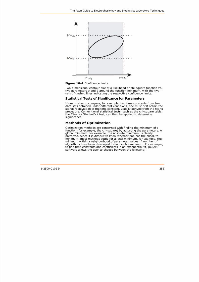
8/13/2019 User Guide v3
http://slidepdf.com/reader/full/user-guide-v3 256/302
1-2500-0102 D 255
the F test or Student s t test, can then be applied to determinesignificance.
Methods of Optimization
Optimization methods are concerned with finding the minimum of afunction (for example, the chi-square) by adjusting the parameters. Aglobal minimum, for example, the absolute minimum, is clearlypreferred. Since it is difficult to know whether one has the absoluteminimum, most methods settle for a local minimum, for example, theminimum within a neighborhood of parameter values. A number ofalgorithms have been developed to find such a minimum. For example,
to find time constants and coefficients in an exponential fit, pCLAMPsoftware allows the user to choose between the following:
Data Analysis
• Minimizing the chi-square using the Levenberg-Marquardtmethod.
• Minimizing the chi-square using the Simplex method.
• Maximizing the likelihood using the variable metric or Simplexmethod.
Of the three methods, the Simplex method is relatively insensitive toshallow local minima. Though it will reliably find the region of the global
minimum or maximum, it may not find the precise location of theminimum or maximum if the function is rather flat in that vicinity. TheLevenberg-Marquardt method is more easily trapped in local minima ofthe function, but it can provide better fits than the Simplex because ituses the mathematical characteristics of the function being minimizedto find the precise location of the minimum or maximum, within thenumerical resolution of the computer. This method also providesstatistical information sufficient to find the confidence limits.
These methods are iterative, for example, they continue refining
parameter values until the function stops changing within a certainconvergence criterion. They also require reasonable starting estimatesfor the parameters, so that the function to be minimized or maximizedis not too far away from its optimum value; a poor starting set can leadsome fit programs to a dead end in a shallow local minimum.
For Boltzmann and exponential fits, the Axon ConventionalElectrophysiology analysis program (Clampfit in the pCLAMP softwaresuite) provides a non-iterative method, in which the data points andfunction to be fit are transformed using a set of orthogonal Chebyshev
polynomials, and the fit function coefficients are quickly calculatedusing these transformed numbers in a linear regression. This method isvery fast and requires no initial guesses, though the parameters maybe slightly different than those found by the methods listed abovebecause the underlying algorithm minimizes a quantity other than thesum of squared differences between fit and data.
References

8/13/2019 User Guide v3
http://slidepdf.com/reader/full/user-guide-v3 257/302
256 1-2500-0102 D
References
Colquhoun, D. and Sigworth, F.J. Fitting and Statistical Analysis ofSingle-Channel Records. in Single-Channel Recording. Sakmann, B. andNeher, E., Eds. Plenum Press, New York, 1983.
Colquhoun, D. and Hawkes, A.G. The Principles of the StochasticInterpretation of Ion-Channel Mechanisms. in Single-ChannelRecording. Sakmann, B. and Neher, E., Eds. Plenum Press, New York,1983.
Dempster, J. Computer Analysis of Electrophysiological Signals.
Academic Press, London, 1993.Eadie, W.T., Drijard, D., James, F.E., Roos, M, Sadoulet, B. StatisticalMethods in Experimental Physics. North-Holland Publishing Co.,Amsterdam, 1971.
The Axon Guide to Electrophysiology and Biophysics Laboratory Techniques
Horn, R. Statistical methods for model discrimination. BiophysicalJournal. 51:255–263, 1987.
McManus, O.B., Blatz, A.L. and Magleby, K.L. Sampling, log binning,fitting, and plotting distributions of open and shut intervals from singlechannels and the effects of noise. Pflugers Arch, 410:530–553, 1987.
Ogden, D.C. Microelectrode electronics. in Microelectrode Techniques.The Plymouth Workshop Handbook. Standen, N.B., Gray, P.T.A. and
Whitaker, M.J., eds.The Company of Biologists Ltd., Cambridge, 1987.
Press, W.H., Flannery, B.P., Teukolsky, S.A. and Vetterling, W.T.Numerical Recipes in C. Cambridge University Press, Cambridge, 1988.
Sachs, F. Automated Analysis of Single-Channel Records. in Single-Channel Recording. Sakmann, B. and Neher, E., Eds. Plenum Press,New York, 1983.
Sigworth, F.J. and Sine, S.M. Data transformations for improved display
and fitting of single-channel dwell time histograms. Biophysical Journal,52:1047–1054, 1987.
Sine, S.M. and Steinbach, J.H. Activation of acetylcholine receptors onclonal mammalian BC3H-1 cells by low concentrations of agonist.Journal of Physiology (London), 373:129–162, 1986.
Wonderlin, W.F., French, R.J. and Arispe, N.J. Recording and analysis ofcurrents from single ion channels. in Neurophysiological Techniques.Basic Methods and Concepts. Boulton, A.A., Baker, G.B. andVanderwolf, C.H., Eds. Humana Press, Clifton, N.J., 1990.

8/13/2019 User Guide v3
http://slidepdf.com/reader/full/user-guide-v3 258/302
1-2500-0102 D 257
Data Analysis

8/13/2019 User Guide v3
http://slidepdf.com/reader/full/user-guide-v3 259/302
258 1-2500-0102 D
11Noise in Electrophysiological
Measurements
In the most general sense, noise can be defined as any disturbancethat interferes with the measurement of the desired signal. Inelectrophysiological measurements, such disturbances can arise fromthe preparation itself, the electrodes that couple the preparation to themeasurement instrument, the electronic instrumentation (for example,voltage-clamp amplifier, patch-clamp amplifier), interference fromexternal sources for example, electrostatic and electromagneticcoupling between the circuitry and 50 or 60 Hz power lines, fluorescentlights, video monitors, acoustic noise, and noise associated withmechanical vibrations), and, if the data is digitized (as is usually thecase), from the digitization process itself (for example, quantizingnoise, aliasing).
We will begin by discussing the basic noise mechanisms that arise fromthe physics of the materials and devices that comprise the electricalsystem. Interference from external sources and noise associated withdigitization will be considered later.
The main fundamental types of noise are: thermal noise, shot noise,dielectric noise, and “excess” noise (for example, 1/f noise). Thesetypes of noise form the basis for a discussion of amplifier noise andelectrode noise.
All the fundamental types of noise are completely random in nature.Their average properties can be measured, but their actual values atany particular instant in time cannot be predicted. The most convenientmeasure of the amplitude of noise is its root-mean-square (rms) value.Many noise processes have a Gaussian distribution of instantaneousamplitudes versus time. The area under the Gaussian distributionrepresents the probability that a noise event of a particular amplitudewill occur (the total area is unity). The probability that a noise peak willexceed plus or minus one times its rms value is 0.32; the probability of

8/13/2019 User Guide v3
http://slidepdf.com/reader/full/user-guide-v3 260/302
1-2500-0102 D 259
p ; p ya particular noise peak exceeding plus or minus three times its rms
value is 0.003. It is common engineering practice to definepeak-to-peak noise as 6 times the rms value; if the noise process hasGaussian distribution, the noise will remain within this bound 99.7% ofthe time. However, peak-to-peak noise is not as clearly defined as isrms noise, and it is not uncommon to find peak-to-peak noiseoperationally defined as anything from 5 times to 8 times rms.
When considering noise in the time domain, it is important to know thebandwidth over which the noise process is observed. Noise is made upof many frequency components, frequently extending from DC to many
megahertz or gigahertz. Some noise processes are naturally restrictedin bandwidth, but most require the appropriate use of filtering torestrict the bandwidth of the noise while allowing adequate resolutionof the signal. When a noise amplitude (rms or peak-to-peak) is
Noise in Electrophysiological Measurements
discussed, it is appropriate to also note the bandwidth over which thenoise is observed and the type of filter that has been used to restrictthe bandwidth.
Due to the random nature of noise, uncorrelated noise sources will addin an rms fashion. Thus if E1, E2, and E3 are the rms values of threeuncorrelated noise sources, the total rms noise, ET, of these sourcestogether is given by:
Because of this relationship, the largest individual source of noise willtend to dominate the total noise. For example, if two noise sources withrms values of 100 μV and 20 μV are added together, the resulting noisewill have an amplitude of {(100 μV)2 + (20 μV)2}1/2 =102 μV rms.
Thermal NoiseThermal noise results from random motion of thermally excited chargecarriers in a conductor. It is often referred to as Johnson noise orNyquist noise. For a resistor, thermal noise can be represented as aseries voltage noise source or a parallel current noise source asillustrated in Figure 11-1. These two representations are equivalent.

8/13/2019 User Guide v3
http://slidepdf.com/reader/full/user-guide-v3 261/302
260 1-2500-0102 D
Figure 11-1 Noise equivalent circuits of a resistor.
The power spectral density (PSD) of thermal noise is white, forexample, it does not vary with frequency. Its value, S2thV, is given as avoltage noise by:
The Axon Guide to Electrophysiology and Biophysics Laboratory Techniques
or, equivalently, as a current noise PSD, S2thI, by:
where k is Boltzmann’s Constant (1.38 x 10⁻²³ J/ °K), T is the absolutetemperature in degrees Kelvin (°K = °C + 273), and R is the resistancein ohms. It should be noted that spectral densities are also often
expressed in units of Volt/√Hz and Amp/√Hz. The variance (also calledthe noise power) over a bandwidth B (units: Hz) is then:
or
The rms noise over a bandwidth B is given by:
or
Spectral densities, rms current and voltage noise for bandwidths of 1and 10 kHz are listed in Table 11-1 for resistances of 100 Ω to 100 GΩ.While thermal voltage noise increases with increasing resistance,thermal current noise decreases as the resistor’s value increases.
Table 11-1 Thermal Noise of Resistors.
1 kHz 10 kHz 1 kHz 10 kHz Voltage Current

8/13/2019 User Guide v3
http://slidepdf.com/reader/full/user-guide-v3 262/302
1-2500-0102 D 261
ResistanceValue
1 kHz
V noise(μV rms)
10 kHz
V noise(μV rms)
1 kHz
I noise(pA rms)
10 kHz
I noise(pA rms)
Voltage
Density(nV/√Hz)
Current
Density(pA/ √ Hz)
100 Ω 0.040 0.126 400 1260 1.26 12.6
1 kΩ 0.126 0.40 126 400 4.0 4.0
10 kΩ 0.4 1.26 40 126 12.6 1.26
100 kΩ 1.26 4.0 12.6 40 40 0.4
1 MΩ 4.0 12.6 4.0 12.6 126 0.126
10 MΩ 12.6 40 1.26 4.0 400 0.040
Noise in Electrophysiological Measurements
Shot Noise
Shot noise arises when current flows across a potential barrier, for
example, a p-n junction in a semiconductor device. Since potentialbarriers are not present in simple resistive elements, resistors do notdisplay shot noise. Over a bandwidth B, the rms value of the shot noisecurrent is given by:
where q is the charge of the elementary charge carrier (for electronsq = 1.6 x 10⁻¹⁹ coulomb) and I is the DC current in Amps.
An important example of shot noise is the equivalent input currentnoise of an operational amplifier that arises from its input bias currentIb (also referred to as gate current for FET1 input devices). For bipolartransistor input devices, Ib is typically in the range of 1 nA to 1 μA; forFET input operational amplifiers, Ib (at room temperature) is typicallyin the range of 1 to 10 pA, and can be less than 0.5 pA for specialdevices. The rms value of shot noise for operational amplifiers with Ib ranging from 0.1 pA to 1 μA in a 1 and 10 kHz bandwidth are listed inTable 11-2. In capacitive-feedback patch voltage-clamp amplifiers (for
l h A h™ 200 i lifi ) h i
100 MΩ 40 126 0.40 1.26 1260 0.0126
1 GΩ 126 400 0.126 0.40 4000 0.004
10 GΩ 400 1260 0 0.04 0.126 12600 0.0013
100 GΩ 1260 4000 0.013 0.040 40000 0.0004
Table 11-1 Thermal Noise of Resistors. (cont’d)
ResistanceValue
1 kHzV noise
(μV rms)
10 kHzV noise
(μV rms)
1 kHzI noise
(pA rms)
10 kHzI noise
(pA rms)
VoltageDensity
(nV/√Hz)
CurrentDensity
(pA/ √ Hz)

8/13/2019 User Guide v3
http://slidepdf.com/reader/full/user-guide-v3 263/302
262 1-2500-0102 D
example, the Axopatch™ 200 series amplifiers), shot noise currentfrom the headstage amplifier sets the noise floor at low-to-moderatefrequencies. By design these devices display very low levels of shotnoise; selected units can have gate currents as low as 0.2 pA, resultingin low-frequency current noise less than that of a 250 GΩ resistor.
1. FET is Field Effect Transistor.
The Axon Guide to Electrophysiology and Biophysics Laboratory Techniques
Dielectric Noise
An ideal lossless capacitor does not produce thermal noise. However, allreal dielectric materials display some loss that results in the generationof thermal noise. For dielectrics with relatively low losses, the spectraldensity of this noise SD2 can be described in terms of the dissipationfactor D and the capacitance CD of the dielectric:
Where f is the frequency in Hz. The PSD of dielectric noisecharacteristically rises linearly with increasing frequency. Thedissipation factor is often listed as tan δe where δe is the loss angle(note that for small δe, tan δe ≈ δe); the “quality factor” Q is theinverse of D (Q = 1/D). For a bandwidth extending from DC to anuppermost cut-off frequency B, the rms noise current ID, resulting froma lossy dielectric, is given by:
Table 11-2 Shot Noise.
Op Amp BiasCurrent
1 kHz Shot Noise(pA rms)
10 kHz Shot Noise(pA rms)
1 μA 18 57
100 nA 5.7 18
10 nA 1.8 5.7
1 nA 0.57 1.8
100 pA 0.18 0.57
10 pA 0.057 0.18
1 pA 0.018 0.057
0.1 pA 0.0057 0.018

8/13/2019 User Guide v3
http://slidepdf.com/reader/full/user-guide-v3 264/302
1-2500-0102 D 263
y , g y
For the best solid dielectrics (for example, quartz, sapphire and someceramics), D is on the order of 10-5 to 10-4. For poorer (lossier)dielectrics D can be much higher; for example, some thermosettingplastics have D in the range of 0.01 to 0.1. For some glasses used tofabricate patch pipettes, D is at least 0.01. The dissipation factor hassome frequency dependence, although in the important range fromabout 1 kHz to 100 kHz it is usually reasonable to approximate it as aconstant. D also shows some temperature dependence (typicallydecreasing with lower temperatures), although again in the usual rangeof temperatures it may be considered constant.
Noise in Electrophysiological Measurements
Dielectric noise is one consideration in the selection of feedback andcompensation capacitors in capacitive-feedback headstages for patchclamping. It must also be considered in the packaging materials,electrode holders, etc. for any high-sensitivity current or chargeamplification device. By using high-quality capacitors (D ≤ 0.0001) thedielectric noise of the feedback and compensation capacitor can bemade a relatively insignificant component of the total noise of presentday capacitive-feedback headstages. For example, using equation (10)
it can be estimated that for D = 0.0001 and CD = 2 pF (1 pF feedbackcapacitor and 1 pF compensation capacitor), the dielectric noise ofthese components in a 10 kHz bandwidth is only about 0.032 pA rms.Dielectric noise associated with packaging (for example, with the inputgate lead of the patch-clamp headstage) can be somewhat higher. Themost important source of dielectric noise in commonelectrophysiological measurements is the dielectric noise of the glassused to fabricate pipettes for patch voltage clamping. This subject willbe considered in greater detail below (see Electrode Noise onpage 268). It is worth noting that a dielectric does not actually have tobe in contact with the input of a sensitive current amplifier, such as apatch-clamp headstage, in order to produce noise. For example, a 1 pFcapacitor formed by a high-loss dielectric with D = 0.1 that is coupledthrough air to the input by a capacitance of 1 pF can result inapproximately 0.35 pA rms in a 10 kHz bandwidth. Thus it is a goodidea both in the design of headstage electronics and of an experimentalpatch clamp set-up not to have exposed, high-loss dielectrics in theimmediate vicinity of the input.
Excess Noise
Excess noise can broadly be defined as any noise that is present in acircuit element in addition to the fundamental noise mechanismsalready described. For example, in the presence of direct current allresistors exhibit low-frequency noise whose power spectral densityvaries inversely with frequency. This noise is present in addition to thethermal noise of the resistor and is usually referred to as “1/f noise.”Different resistor types display different amounts of 1/f noise with

8/13/2019 User Guide v3
http://slidepdf.com/reader/full/user-guide-v3 265/302
264 1-2500-0102 D
Different resistor types display different amounts of 1/f noise, withmetal film and wirewound types showing the least excesslow-frequency noise and carbon composition resistors showing themost. The PSD (in V2 /Hz) of this excess noise rises with decreasingfrequency essentially as 1/f. Its magnitude is directly proportional tothe DC current flowing through the resistor. Semiconductor devices alsoexhibit 1/f noise.
High-value (gigaohm range) resistors, such as those used as thefeedback element in resistive-feedback patch-clamp headstages, alsodisplay a form of excess noise that rises with increasing frequency.Generally, such resistors only achieve their thermal noise level (which isthe minimum possible) in the frequency range from about 10 Hz to1 kHz. At low frequencies, 1/f noise is observed, and at high
The Axon Guide to Electrophysiology and Biophysics Laboratory Techniques
frequencies the noise PSD typically rises as f α, where α is usually inthe range of 1 to 2. This noise can result in rms noise from a resistorhaving several times the predicted thermal noise value in a 10 kHzbandwidth. The elimination of this noise source is one of themotivations behind using capacitive-feedback in patch clamps such asthe Axopatch 200 series amplifiers.
Amplifier NoiseThe intrinsic noise of an operational amplifier can be described by anequivalent input voltage noise En in series with the negative (-) inputand an equivalent input current noise In between the positive (+) andnegative (-) inputs (see Figure 11-2). These noise sources have beenreferred to the input for convenience of analysis. It should be noted,however, that they are measured at the output. For example, in anopen-loop situation (such as shown in (Figure 11-2), if the inputs aregrounded, the voltage at the negative (-) input will be zero (ground). En must be inferred by measuring the output noise voltage and dividing itby the open-loop gain (both are frequency dependent) of the amplifier.On the other hand, in a closed-loop situation (which is always the casewhen using operational amplifiers, as illustrated in Figure 11-3), En willactually appear at the negative (-) input due to the action of thefeedback loop.

8/13/2019 User Guide v3
http://slidepdf.com/reader/full/user-guide-v3 266/302
1-2500-0102 D 265
Figure 11-2 Operational amplifier noise model.
Noise in Electrophysiological Measurements
Figure 11-3 Noise model of a simplifier current-to-voltage converter.
When analyzing the noise of an operational circuit it is convenient toconsider the noise sources in terms of their power spectral densities. Inthis case the noise sources will be denoted by lower case symbols, forexample, en(f) (units: V/ √ Hz) or en 2(f) (units: V2 /Hz). As a usefulexample of noise analysis in an operational circuit, consider thesimplified current-to-voltage converter illustrated in Figure 11-3. In this
circuit en and in are the input voltage and current noise PSDs,respectively, and ef is the PSD of the noise (thermal and excess) of thefeedback resistor Rf . The current to be measured is introduced at theterminal labeled “input.” For simplicity, the positive (+) input is shownto be grounded. Cg is any capacitance between the negative (-) inputand ground; this includes the input capacitance of the amplifier plusstrays and is usually about 15 pF. The noise PSD at the output of the IVconverter, Sout 2(f), can be shown to be:

8/13/2019 User Guide v3
http://slidepdf.com/reader/full/user-guide-v3 267/302
266 1-2500-0102 D
It is useful to present this result in terms of current so it can becompared directly with the current signal being measured. This isaccomplished by dividing the above expression by Rf 2, thus referringthe noise to the input. The input referred PSD, Sin 2(f), is then given by:
In general, in, en and ef are all functions of frequency: in is the shotnoise of the input gate current of the amplifier but usually displays
The Axon Guide to Electrophysiology and Biophysics Laboratory Techniques
some 1/f behavior at low frequencies; ef is the thermal and excessnoise of Rf ; and en also displays 1/f behavior at low-to-moderatefrequencies. Nevertheless, it is convenient to assume that each of theseterms is independent of frequency so that equation (12) can be easilyintegrated over a frequency band (for instance, DC to some uppermostbandwidth denoted by B). The square root of this result is then the rmsnoise for the bandwidth B:
It should be noted that if it is assumed that ef is only the thermal noiseof the feedback resistor, then the term ef 2 /Rf 2 is simply 4kT/Rf (seeequation (3) above).
It is instructive to consider the relative magnitudes of the various terms
in equation (12) or (13). In the case of a patch voltage clamp, thevalue of Rf is selected to be very high, both to provide adequate gain toresolve tiny (pA) currents and to minimize the noise contribution of thisresistor; 50 GΩ is common for single-channel recording. The PSD ofthe thermal noise of an ideal 50 GΩ resistor is 3.2 x 10⁻³¹ Amp2 /Hz andthe rms noise associated with such a component over a bandwidth of10 kHz is 0.057 pA rms (although as already noted, excesshigh-frequency noise can increase this value several fold). The shotnoise, which accounts for in, associated with an input gate current of
0.2 pA would, by itself, produce noise of about 0.025 pA rms in a10 kHz bandwidth. For a typical high-quality patch-clamp headstage, en is about 2–3 nV/ √ Hz at frequencies above about 1 kHz; Cg is usually
about 15–20 pF. With these values, the term amounts
to roughly 0.15 pA rms in a 10 kHz bandwidth. These three termsshould be uncorrelated; therefore, they sum in an rms fashion so thatthe total predicted noise is (0.0572 + 0.0252 + 0.152)1/2 = 0.162 pArms. For a resistive-feedback headstage, actual noise in a 10 kHz

8/13/2019 User Guide v3
http://slidepdf.com/reader/full/user-guide-v3 268/302
1-2500-0102 D 267
bandwidth is normally substantially higher (about 0.25–0.30 pA rms)both because of excess noise from the feedback resistor and because ofthe characteristics of the low-pass filters that do not abruptly cut offnoise at the -3dB bandwidth (Filtering on page 287). Nevertheless, it isimportant to note that for bandwidths above a few kilohertz, the termarising from en and Cg dominates total noise. To intuitively understandthe origin of this term, it is only required to remember that the currentthrough a capacitor is directly proportional to the rate of change ofvoltage across the capacitor (I = C(dV/dt)). Therefore, the voltagenoise at the negative (-) input of the amplifier produces current noisethrough the capacitor Cg. This noise increases with increasing frequencysimply because higher frequency components of the voltage noiseinvolve more rapidly changing voltages. The noise current through the
8/13/2019 User Guide v3
http://slidepdf.com/reader/full/user-guide-v3 269/302
The Axon Guide to Electrophysiology and Biophysics Laboratory Techniques
mechanism alone. Obviously, from the point of view of noise, it isimportant to minimize the capacitance of the holder and pipette.
Dielectric Noise
The basic characteristics of dielectric noise have already been describedabove (see equations (9) and (10)). Dielectric noise of the pipette canbe a major contributor to total noise in patch voltage clamping; in somesituations it can be the dominant noise source. The dielectric noisearising from the pipette depends on the dissipation factor D of the glassused to fabricate the pipette, on the pipette capacitance (CD inequations (9) and (10)), and on the presence of Sylgard coating. Thedissipation factor D of glasses other than quartz that have beensuccessfully used for patch pipettes generally falls in the ranges of0.001–0.01. The dissipation factor for quartz is variously reported to be10-5 to as much as 4 x 10⁻⁴. For Amersil T-08 quartz, which has beenused in all of the preliminary tests of quartz pipettes described below,the reported dissipation factor is 10-4. For uncoated pipettes the value
of CD is determined by the dielectric constant ε of the glass, the ratioof the outer diameter (OD) to the inner diameter (ID) of the pipette,the depth of immersion of the pipette into the bath, and to some extentby the pulling characteristics of the glass and the geometry near its tip.The dielectric constant ranges from as little as 3.8 for quartz to morethan 9 for some high-lead glasses. Typical glass capillaries used in thefabrication of patch pipettes have an OD of 1.65 mm and an ID of1.15 mm; thus OD/ID ≈ 1.43. If it is assumed that these proportions(OD/ID = 1.43) are maintained as the glass is drawn out in pulling,then for uncoated pipettes the value of CD will be approximately0.15 εpF per mm of immersion into the bath. For thick-walled glasswith OD/ID = 2, this value would fall to 0.08 pF per mm of immersion;while for thin-walled glass with OD/ID = 1.2 the capacitance wouldincrease to about 0.30 εpF per mm.
Actual measurements with uncoated or lightly Sylgard-coated pipettesfabricated from glasses with known ε and immersed to a depth of2–3 mm indicate that these values often underestimate pipettecapacitance; therefore, the dielectric noise is also underestimated. This

8/13/2019 User Guide v3
http://slidepdf.com/reader/full/user-guide-v3 270/302
1-2500-0102 D 269
is probably due to non-uniform thinning near the tip and to someuncertainty as to the true depth of immersion (due to a meniscus ofsolution around the pipette). For example, using the popular Corning7052 glass, which has ε = 4.9 and with OD/ID ≈ 1.43, it is notuncommon to measure a pipette capacitance as high as ≈ 3 pF, forexample, about twice the predicted value, when an uncoated pipette ora pipette very lightly coated with Sylgard is immersed at a depth of2 mm.
Despite this precautionary note, it is clear that, all else being equal, the
value of CD varies linearly with the dielectric constant ε of the glass.Equation (10) indicates that if the depth of immersion and the OD/IDratio are constant, the rms noise for a given bandwidth arising from thelossy dielectric characteristics of pipettes fabricated from various
Noise in Electrophysiological Measurements
glasses will be proportional to (Dε)1/2. Thus the lowest noise glassesare expected to be those that minimize the product of the dissipationfactor and the dielectric constant. This relationship has been born outexperimentally in tests of some 20 different types of glass used tofabricate patch pipettes (Rae and Levis, Personal Communication).
To illustrate the range of results expected for different glass types, wewill consider three pipettes with identical geometry fabricated fromthree different glasses. It will be assumed that OD/ID ≈ 1.4,
CD = 0.2 εpF per mm of immersion, the immersion depth is 2 mm, thepipettes are uncoated or are coated very lightly with Sylgard (so thatthe coating does not reduce the dielectric noise significantly), and therms noise is measured at a 10 kHz bandwidth (-3 dB, 8-pole Besselfilter). Corning 7052 glass (D ≈ 0.003 and ε ≈ 5) representsreasonably low-loss glasses used to fabricate patch pipettes. Under theabove stated conditions, the CD value of this pipette is 2 pF and thedielectric noise contribution predicted by equation 10 is about 0.17 pArms, or about 0.2 pA rms if the characteristics of an 8-pole Bessel filter
are taken into account. On the other hand, 0080 soda lime glass(D ≈ 0.01, ε ≈ 7) represents high-loss glasses, which were commonlyused in the early days of patch clamping. Its CD = 2.8 pF and dielectricnoise of about 0.44 pA rms is predicted. Finally, Corning 7760 is a verylow-loss glass with D ≈ 0.0017 and ε ≈ 4.5. With CD = 1.8 pF, adielectric noise of slightly less than 0.15 pA rms is predicted. Thesefigures are in reasonable agreement with experimental findings thathave attempted to separate the components of total noise arising fromthe dielectric noise of pipettes fabricated from various glasses.
Since the capacitance CD increases approximately linearly withincreasing depth of immersion, the dielectric noise for any particulartype of glass and OD/ID ratio should vary approximately as the squareroot of the depth immersion. From the point of view of noise reduction,it is clearly useful with excised patches to withdraw the pipette tip asclose to the surface of the bath as possible. If the patch cannot beexcised, then the bath should be as shallow as possible. For example,for a pipette fabricated from Corning 7760, as in the previous example,dielectric noise is expected to decrease from about 0.15 pA rms in a

8/13/2019 User Guide v3
http://slidepdf.com/reader/full/user-guide-v3 271/302
270 1-2500-0102 D
10 kHz bandwidth for a 2 mm immersion depth to roughly 0.05 pA rmsfor a 0.2 mm immersion depth. The effect of immersion depth onpipette noise has, at least qualitatively, been verified experimentally. Amethod employing Silicone fluid to minimize the effective pipetteimmersion depth was introduced by Rae and Levis (1992) and isdescribed below.
The above discussion dealt with expected behavior for uncoatedpipettes. However, it is common practice (and highly recommended forlow-noise measurements) to apply a coating of Sylgard #184 covering
the entire tapered region of the pipettes (for example, approx.5–10 mm) and extending to within roughly 100 μm of the tip (seeChapter 4: Microelectrodes and Micropipettes on page 117). Coatingwith a hydrophobic substance such as Sylgard is necessary to prevent
The Axon Guide to Electrophysiology and Biophysics Laboratory Techniques
the formation of a thin film of solution that will creep up the outer wallof an uncoated pipette. Such a film can produce very large amounts ofnoise in uncoated pipettes. Sylgard coating not only virtually eliminatesthis noise source but also thickens the wall of the pipette therebyreducing its capacitance. The dielectric constant of Sylgard #184 is 2.9and its dissipation factor is ≈ 0.002, which is lower than that of mostglasses that have been used for patch pipette fabrication. Thus, coatingwith Sylgard will reduce dielectric noise of patch pipettes. It is expected
that the improvement in noise associated with Sylgard coating will begreatest for glasses with a high D product (for example, soda limeglass); this has been confirmed experimentally. Improvement of noiseshould be less for glasses with very low values of D, but coating withSylgard will reduce the dielectric noise of all glasses. The effects ofSylgard coating on noise are, however, difficult to quantify theoreticallyprimarily because the thickness of the coating is usually not uniform. Inparticular, it is difficult to achieve a very thick coating very near the tip.
Experimental tests of the noise properties of patch pipettes fabricated
from 19 different kinds of glass (see Chapter 11: Noise inElectrophysiological Measurements on page 259) have confirmed thegeneral conclusions described above. With few exceptions, the noiseattributable to the pipette is inversely correlated with the D product ofthe glass. In addition, thicker-walled pipettes and shallow depths ofimmersion reduce noise for any particular glass type. Sylgard coatinghas its greatest effect on the glasses with the poorest inherentelectrical properties, but it is important to remember that such coatingis necessary for all types of glass.
It has been obvious for some time that pipettes fabricated from quartzshould produce only very small amounts of dielectric noise due to thelow dielectric constant of quartz (ε = 3.8) and, more importantly, itsextremely low dissipation factor (D ≈ 10-5 – 10-4). However, due to thehigh melting point of quartz (≈ 1600 °C), only with the advent ofautomated laser pullers has it become practical to pull patch pipettesfrom quartz tubing. A quartz pipette with D = 10-4 that is immersed to adepth of 2 mm (again assuming 0.2 εpF per mm of immersion) wouldbe predicted to produce only about 0.03 pA rms of dielectric noise in abandwidth of 10 kHz (-3 dB, 8-pole Bessel filter); for D = 10-5 this
l ld f ll t 0 01 A P li i t i

8/13/2019 User Guide v3
http://slidepdf.com/reader/full/user-guide-v3 272/302
1-2500-0102 D 271
value would fall to 0.01 pA rms. Preliminary measurements usingAmersil T-08 quartz suggest that the amount of dielectric noise in thissituation is closer to 0.04–0.05 pA rms. A more detailed discussion ofpreliminary estimates of the noise properties of quartz pipettes isprovided below.
Dielectric noise is probably the largest source of noise for pipettesfabricated from all glasses other than quartz. For pipettes fabricatedfrom quartz, due to its very low dissipation factor, sources of noiseother than dielectric noise are expected to dominate total pipette noise
(See Noise Properties of Quartz Patch Pipettes on page 275).To summarize, dielectric noise can be minimized by using thick-walledglasses with low values of D and coating the pipette with Sylgard #184.
Noise in Electrophysiological Measurements
The effects of Sylgard coating are greatest for glasses with relativelypoor electrical properties. For excised patches, dielectric noise can beminimized by withdrawing the tip of the pipette as close as possible tothe surface of the bath.
It should be noted that dielectric noise will also contribute to the noiseassociated with the holder. For an Axopatch 200A amplifier with anopen circuit noise of 0.06 pA rms in a 5 kHz bandwidth, total noiseshould not increase to more than about 0.07 pA rms in this bandwidth
when the Axon-supplied polycarbonate holder is attached. Part of thisnoise increment is due to the fact that the holder adds about 1–1.5 pFof capacitance to the headstage input. The rest of the increment innoise associated with the holder is presumably dielectric noise, whichcan be estimated to account for roughly 0.03 pA rms in a 5 kHzbandwidth.
Noise Arising From Distributed Pipette Resistance andCapacitance
Most of the resistance of a patch pipette resides at or very near its tip.On the other hand, the capacitance of an uncoated pipette can beexpected to vary linearly with its depth of immersion into the bath.Therefore, it has sometimes been assumed that current noise arisingfrom the thermal voltage noise of the pipette resistance in conjunctionwith the pipette capacitance can be assumed to be negligible incomparison with other noise sources. However, significant resistanceresides in regions of the pipette that are further removed from the tip.The thermal voltage noise of this resistance will greatly exceed the
input voltage noise of the headstage itself, with which it is in series. Theactual situation is complicated because both the pipette resistance andcapacitance are distributed. In this section we will consider the pipettecapacitance to be lossless, and initially the effects of Sylgard coatingwill not be considered. In order to estimate the noise arising from thedistributed pipette resistance and capacitance, we will consider ratheridealized pipette geometry.
The pipette has been modeled as a shank and a conical regionapproaching the tip; the angle of the cone is 11.4° and the tip opening
is 1 μm in diameter With this cone angle the ID of the pipette increases

8/13/2019 User Guide v3
http://slidepdf.com/reader/full/user-guide-v3 273/302
272 1-2500-0102 D
is 1 μm in diameter. With this cone angle the ID of the pipette increasesto 100 μm at a distance of 0.5 mm from the tip, 200 μm at a distanceof 1 mm from the tip, 300 μm at a distance 1.5 mm from the tip, etc.When filled with a solution with a resistivity of 50 Ωcm the pipette willhave a total resistance of about 3.2 MΩ. About 2.1 MΩ of this totalresistance resides in the first 10 μm from the tip; slightly more than3 MΩ occurs in the first 100 μm from the tip. However, about 80 kΩresides in the region from 100–200 μm from the tip, an additional27 kΩ resides in the region from 200–300 μm; and about 37 kΩ occurs
in the region from 300 μm to 1 mm from the tip. The region from1–4 mm from the tip adds another 12 kΩ. It has been assumed thatthe capacitance is uniformly distributed along the pipette with a valueof 1 pF/mm of immersion. An Ag/AgCl wire extends into the pipette
The Axon Guide to Electrophysiology and Biophysics Laboratory Techniques
coming to within 4 mm of the tip and it is assumed that the resistanceof the pipette is negligible beyond the tip of the wire (due to theshunting effect of the wire). A noise equivalent circuit of the pipette canbe created by lumping the resistance and capacitance of each smallsegment (for example, 20–50 μm) of pipette. The approximate circuitis then a ladder network formed of a series of resistors and theirequivalent thermal voltage noise sources with a capacitor to ground ateach node representing a portion of the pipette immersed in the bath.
Rough calculations with such an equivalent circuit indicate that for adepth of immersion of 2 mm the noise arising from this mechanism willbe about 0.13 pA rms in a 10 kHz bandwidth. For a 1 mm depth ofimmersion this value would fall to about 0.10 pA rms. For an idealizedpipette identical to the one described here but with a cone angle of22.6° (total resistance is about 1.6 MΩ) these values fall to about0.07 pA rms for a 2 mm depth of immersion and about 0.05 pA rms fora 1 mm depth of immersion, both for a 10 kHz bandwidth. Over thefrequency range of interest to patch voltage clamping, the PSD(Amp2 /Hz) of this noise should rise with increasing frequency as f 2.
These calculated values are highly approximate and the assumedgeometry is obviously an over-simplification. A variety of factors couldincrease the noise arising from this mechanism. For example, the noiseshould increase if there is an extended region behind the tip where theangle of taper is quite shallow, resulting in increased resistance in thisregion. Noise will also increase if the wire does not protrude as close tothe tip as assumed above. In addition, some glasses tend to thin nearthe pipette tip, resulting in increased capacitance in this region. Itshould also be noted that shallow depths of immersion would notdecrease this noise quite as much as might be expected since thiswould decrease the pipette capacitance, but not its resistance.
The noise from this mechanism can be reduced in several ways. Fromthe above estimates it seems that noise arising from the distributedresistance and capacitance of the pipette should be smaller than thedielectric noise of pipettes fabricated from even the best knownglasses. Nevertheless, with better (lower loss) glasses, particularlyquartz, this mechanism could be the dominant source of noise from thepipette itself, and its reduction may become important. First, it is
obvious that the geometry of the first few millimeters of the pipette will
8/13/2019 User Guide v3
http://slidepdf.com/reader/full/user-guide-v3 274/302
1-2500-0102 D 273
obvious that the geometry of the first few millimeters of the pipette willbe an important determinant of the magnitude of this noise; therefore,when possible, pipettes should be pulled to minimize the resistancedistal to the tip. Anything that reduces the pipette capacitance per unitlength will also reduce this noise. Thus, thick-walled pipettes andglasses with low dielectric constants should provide the best results interms of noise. Perhaps of more practical importance, coating thepipette with Sylgard #184 can significantly reduce the pipettecapacitance, and consequently reduce noise of the type considered
here. However, as already noted, it is more difficult to build up a thickcoat of Sylgard in the region within the first few hundred micrometersfrom the tip than in more distant regions. As was the case withdielectric noise, shallow depths of immersion will also reduce the noise
Noise in Electrophysiological Measurements
arising from pipette resistance and capacitance. Finally, it should alsobe possible to reduce this noise regardless of the immersion depth byusing a fine wire (Ag/AgCl or platinized Ag/AgCl possibly sharpened atthe tip) that protrudes as far as possible toward the tip of the pipette.Such a wire will, in effect, short out (in a frequency-dependent fashion)the resistance of the pipette-filling solution in the region into which itextends; thus, while the pipette capacitance will be unaltered for anygiven depth of immersion, its resistance up to the end of the wire would
be significantly reduced.In 1992, Rae and Levis have introduced a technique that has beenshown to minimize pipette noise arising from all of the mechanismsdiscussed above. In this technique, the surface of the bathing solutionwas covered with a layer of Silicone oil (#200 Fluid from Dow Corning,Midland, MI). With excised patches it was then possible to raise the tipof the electrode to within a few micrometers of the saline-oil interface;a sharp line of demarcation could be observed along the pipette at thisinterface. The electrical characteristics of this oil are apparently quitegood2, so that only the tip of the pipette that remains in saline appearsto contribute to total noise. If 10 μm of the pipette tip remain in saline,it would be expected that the capacitance associated with this lengthshould be roughly 0.01 pF. Dielectric noise associated with theimmersed portion of the pipette should be about one tenth of thevalues predicted for a 1 mm depth of immersion. It should bereasonable to approximate distributed R-C noise in this situation by alumped resistance equal to the resistance of the pipette other than thatarising from the tip itself is series with approximately 0.01 pF. If thisresistance is taken to be 2.5 MΩ, the expected noise is only about 7 fA
rms in a 10 kHz bandwidth; even for 10 MΩ it is less that 15 fA rms inthis bandwidth. The noise increment associated with the pipettecapacitance and the headstage input voltage noise is also minimized inthis arrangement since the capacitance remains essentially the same asthat with the electrode in air. It should also be noted that even whenpatches cannot be excised, this approach can still be effective if thebath is designed so that the solution level can be lowered, therebybringing the layer of silicone fluid very close to the cell surface.
Using quartz pipettes with this technique has resulted in noise levels in
actual recording situations as low as 0 08 pA rms in a 5 kHz bandwidth

8/13/2019 User Guide v3
http://slidepdf.com/reader/full/user-guide-v3 275/302
274 1-2500-0102 D
actual recording situations as low as 0.08 pA rms in a 5 kHz bandwidth(4-pole Butterworth filter). For these experiments, the Axopatch 200Aamplifier was used with an open-circuit headstage noise of 0.057 pArms in a 5 kHz bandwidth; with the holder and electrode attached, butwith the electrode tip in air, noise typically increased to about 0.07 pArms in this bandwidth.
2. Although the dielectric characteristics of the specific Silicone fluid used in these
experiments is not available, Table 2.5 of Electronics Designers' Handbook(1977, L. Giacoleto ed., McGraw-Hill) lists a dissipation factor (D) of 8.5x10⁻⁵ at
1 kHz and 2x10⁻⁵ at 100 kHz for Silicone fluid (methyl- or ethyl-siloxane
polymer); the dielectric constant ε is 2.68.
The Axon Guide to Electrophysiology and Biophysics Laboratory Techniques
In several experiments it was shown that the total noise closelyapproximated the rms sum of the noise of the headstage plusholder/electrode (electrode in air) and the thermal current noise of themeasured DC seal resistance. This implies that dielectric noise and “distributed R-C noise” of the pipette contributed only a negligibleamount to total noise in this situation. Rae and Levis (1993) showedthat quartz pipettes can be fabricated with the Sutter Instrument P-200laser-based puller to yield lower noise than they previously achieved,
obviating the need for Silicone oil.Preliminary tests have also been made using this technique withpipettes fabricated from two other types of glass (Corning 7760, KimbleKG-12). Although the noise reduction was significant, results werenever as good as those achieved with quartz. For example, the bestresults achieved with KG-12 were slightly more that 0.10 pA rms in a5 kHz bandwidth, even when seal resistances in the range of50–100 GΩ were obtained. For a total noise of 0.105 pA rms, andassuming that the headstage plus holder/electrode in air produced
0.075 pA rms and that a 50 GΩ seal produces 0.04 pA rms, all in a5 kHz bandwidth, the pipette would be estimated to contribute about0.06 pA rms in this bandwidth. On the basis of the above discussion,this is several times the amount of noise expected for a pipettefabricated from this glass with 10 μm of its tip in saline. One possibleexplanation of at least part of this discrepancy would be to assume thatthe glass had thinned excessively near the tip. It is also possible thatthe noise attributed to the seal in arriving at this estimate is too low.More work will be needed to clarify this issue.
Noise Properties of Quartz Patch PipettesSince 1991, it is now possible to routinely fabricate patch pipettes fromquartz using the Model P-2000 puller from Sutter Instrument Company(Novato, CA). This puller uses a laser to overcome the extremely highmelting temperatures needed to draw pipettes from quartz tubing.Preliminary results were made using Amersil T-08 quartz pipettesalthough, it was difficult to pull small-tipped blunt pipettes with1.65 mm OD 1.15 mm ID tubing. Pipettes fabricated from this tubingtypically had a rather long and relatively narrow shank. This geometryis not ideal for the lowest possible noise. Even so, these pipettes

8/13/2019 User Guide v3
http://slidepdf.com/reader/full/user-guide-v3 276/302
1-2500-0102 D 275
is not ideal for the lowest possible noise. Even so, these pipettesproduced significantly less noise than pipettes fabricated from the bestglasses used previously (for example, 7760, 8161). In actual recordingsituations with pipettes immersed about 3 mm into the bath and with sealresistances ≥ 50 GΩ, rms noise in a 5 kHz bandwidth was typicallyabout 0.12–0.13 pA rms using an Axopatch 200A amplifier. Estimatesof the contribution of the pipette to this noise were in the range of0.075–0.09 pA rms in this bandwidth. With the new techniquedescribed above (Rae & Levis, 1992), which allows the pipette tip to bepositioned within a few micrometers of a layer of Silicone oil coveringthe surface of the bath, background noise levels as low as 0.08 pA rmsin a 5 kHz bandwidth have been achieved in actual single-channel
Noise in Electrophysiological Measurements
recording situations with quartz pipettes. In such cases the contributionof the dielectric noise and distributed R-C noise of the pipette appearsto be negligible in comparison to other noise sources.
More accurate estimates of the noise attributable to the pipette couldbe made by sealing quartz pipettes to Sylgard. A typical result forapproximately a 3 hmm depth of immersion is 0.115 pA rms in a 5 kHzbandwidth for pipettes coated with a thin layer of Sylgard to withinabout 100–200 μm of the tip. The power spectral density (PSD) of this
noise was also measured. An estimate of the PSD attributable to thedielectric noise and distributed R-C noise of the pipette was obtained bysubtracting from the total PSD the PSD of the headstage with theelectrode in air with a correction made for the effects of the additionalcapacitance of the immersed pipette (about 2.6 pF) in conjunction withthe headstage input voltage noise. The thermal current noise levelassociated with the DC seal was also subtracted. The resulting PSD wastaken to be the best estimate of the noise attributable to the pipetteper se. This PSD (Amp2 /Hz) increased with frequency with a slope ofapproximately f 1.85 in the frequency range from 2–20 kHz. From thePSD it could be estimated that the pipette accounted for about 0.07 pArms of noise in a 5 kHz band width and about 0.17 pA rms in a 10 kHzbandwidth. If it is assumed that the slope of f 1.85 was composed of acomponent with a slope of f attributable to the dielectric noise of thepipette and a component with a slope of f 2, attributed to distributedresistance-capacitance noise of the pipette, it can be estimated thatdielectric noise would account for slightly less than 0.06 pA rms in a10 kHz bandwidth. Distributed R-C noise would then account for about0.16 pA rms at this bandwidth. The estimated value of dielectric noiseis somewhat higher than would be expected from the value of D listedfor Amersil TO-8 quartz (0.0001 at 1 MHz) and the measured value ofCD (2.6 pF); with these values, equation 10 predicts ≈ 0.04 pA rms ofdielectric noise in a 10 kHz bandwidth. If the above parsing of the noisecomponents is correct, then it can be estimated that the actual value ofD for the quartz used was closer to 0.00025. Even if this value is correct,the Dε product for this quartz is still about an order of magnitude lowerthan that of any other glass used to date for the fabrication of patch
pipettes. At the time of this writing, neither different grades (forexample, higher purity) of quartz from the same supplier nor quartz

8/13/2019 User Guide v3
http://slidepdf.com/reader/full/user-guide-v3 277/302
276 1-2500-0102 D
p p g, g (p , g p y) q pp qfrom other manufacturers have been investigated. It should also benoted that the noise component attributed to distributed R-C noiseprobably could have been reduced if the pipettes tested had a morefavorable geometry.
When the same procedure was used to estimate the pipette noise whenthe depth of immersion was decreased such that the increment incapacitance was about 0.7 pF above that measured with the pipette tip just above the solution, it was found that the noise attributable to thepipette was roughly a factor of two lower than the figures reportedabove. In this case the estimated pipette noise PSD increased withincreasing frequency approximately as f 1.9 in the range from 2–20 kHz.
The Axon Guide to Electrophysiology and Biophysics Laboratory Techniques
This is consistent with the prediction that the relative decrease indielectric noise will be somewhat greater than that of distributed R-Cnoise as the depth of immersion decreases.
It should be noted that the results for quartz pipettes are qualitativelyas well as quantitatively different from those that have been obtainedpreviously from pipettes fabricated with other types of glass. Estimatesof pipette noise based on procedures like those described above havebeen performed for many types of glass (for example, Figure 11.4). Even
for the lowest Dε product glasses (for example, 7760, 8161, 7740), theestimated pipette noise PSD rises with increasing frequency as f 1.1– f 1.3
(frequency range 2–20 kHz, immersion depth ≈ 2 mm). This indicatesthat dielectric noise dominates total pipette noise for these glasses.However, for quartz not only is the pipette noise significantly less for agiven depth of immersion, but the estimated pipette noise PSD risesmuch more steeply with increasing frequency (f 1.8 – f 1.9 in the 2–20 kHzfrequency range)3. This indicates that dielectric noise is no longer thedominant source of noise for patch pipettes fabricated from quartz. The
data described above are consistent with the interpretation that forquartz pipettes “distributed R-C noise” has become the dominant noisemechanism due to the greatly reduced contribution of dielectric noise.As more data from quartz pipettes becomes available these estimatesand conclusions will doubtlessly be refined.
Noise Arising From Pipette Resistance and PatchCapacitance
The capacitance, Cp, of the patch is in series with the entire pipetteresistance, Re. The thermal voltage noise of Re will produce currentnoise in conjunction with the patch capacitance. The PSD of this noise,S2p (f), is given by:
where e2e = 4kTR e is the thermal voltage noise of the pipette. The rms noise arising from this mechanism from DC to a bandwidth B is then

8/13/2019 User Guide v3
http://slidepdf.com/reader/full/user-guide-v3 278/302
1-2500-0102 D 277
3. Note, however, that the PSD for quartz pipettes is lower than that of pipettes
made from other glasses at all frequencies measured. At sufficiently high
frequencies distributed R-C noise should dominate the total noise for pipettes
fabricated from any type of glass. However, for quartz pipettes the PSD of
distributed R-C noise should exceed that of dielectric noise by 1 kHz; for pipettes
made from 7760, distributed R-C noise should not exceed dielectric noise up to
10–20 kHz, and for soda lime (for example, 0080) pipettes this frequency might
be closer to 100 kHz or more. Distributed R-C noise depends on the pipettegeometry and a variety of other factors already described; the only influence of
the glass type itself—accept in so far as it effects the geometry which can be
pulled—is its dielectric constant.
Noise in Electrophysiological Measurements
. In general, this noise should be quite small, but it canbecome significant when the patch area is large; for example, when alarge “bleb” of membrane is sucked into the pipette tip. Sakmann andNeher (1983, in Single-Channel Recording, Sakmann, B. and Neher E.eds. pp. 37–51) measured patch capacitance for a large number ofpipettes with resistances ranging from about 1–10 MΩ. They found thatthe value of Cp varied from as little as 0.01 pF to as much as 0.25 pF.
Despite a very large amount of scatter, they found that Cp and Re werecorrelated, with Cp increasing as Re decreases. The best fit to their datawas Cp = 0.126 pF(1/R + 0.018), where R is the pipette resistance inMΩ. Using this average relationship it can be predicted that for a “typical” 10 MΩ pipette (Cp = 0.015 pF) the noise in a 10 kHzbandwidth (8-pole Bessel filter) arising from this mechanism will beabout 0.03 pA rms, while for a 1 MΩ pipette (typical Cp = 0.128 pF) thisvalue will increase to 0.08 pA rms. Sakmann and Neher’s resultsindicate that in the most favorable situations in terms of “Re-Cp” noise,
the rms noise from this mechanism can be as low as 0.01 pA rms in a10 kHz bandwidth. However, in the least favorable situation (Re ≈ 2MΩ, Cp ≈ 0.25 pF) the noise from this mechanism can be as large as0.23 pA rms in a 10 kHz bandwidth (8-pole Bessel filter).
Seal Noise
The membrane-to-glass seal that is essential to the patch voltage-
clamp technique is the final source of noise associated with the pipettethat will be considered here. Seal noise is perhaps the least understoodsource of noise in the patch clamp technique. The power spectral,S2sh(f), of the noise arising from the seal for zero applied voltage isgiven by:
where Re{Ysh} is the real part of the seal admittance Ysh. The minimumestimate of seal noise results from the assumption that
Re{Ysh} = 1/Rsh, where Rsh is the DC seal resistance. If this assumptionis correct then for a 10 kHz bandwidth seal resistances of 1 10 and

8/13/2019 User Guide v3
http://slidepdf.com/reader/full/user-guide-v3 279/302
278 1-2500-0102 D
is correct, then for a 10 kHz bandwidth, seal resistances of 1, 10 and100 GΩ would produce noise of 0.4, 0.13 and 0.04 pA rms,respectively. Since values of Rsh in the range of 100–200 GΩ are notuncommon, this would imply that the noise associated with a very tightseal would be small in comparison with other sources of patch-clampnoise. However, it is possible that the PSD of seal noise may rise abovethe minimum level given by 4kT/Rsh as frequency increases (forexample, the real part of the seal admittance may increase with
frequency) due to the capacitance of the glass and the membranewhich make up the wall of the seal. Unfortunately, we have no goodtheoretical basis upon which to estimate Ysh since the precise nature ofthe membrane-glass seal is not known.

8/13/2019 User Guide v3
http://slidepdf.com/reader/full/user-guide-v3 280/302
Noise in Electrophysiological Measurements
and cell capacitance, series-resistance compensation is required toincrease the actual bandwidth of current measurement beyond1/2πRsCm. The level of series-resistance compensation is an importantdeterminant of whole-cell voltage clamp noise as well as of thebandwidth and fidelity of recording (see Series-ResistanceCompensation on page 86). The voltage noise PSD of Rs isapproximated by 4kTRs (V2 /Hz). It should be noted, however, that inaddition to thermal noise a 1/f component is expected, particularly
when relatively large currents are passed through the pipette. The PSD,S2wc (f), of the current noise arising from Rs and Cm is given by:
where e2s = 4kTRs and τsr = RsrCm and Rsr is the residual (i.e.,uncompensated) series resistance, for example, if Rs = 10 MΩ then forseries-resistance compensation levels of 50%, 70% and 90%, Rsr will
be 5 MΩ
, 3 MΩ
and 1 MΩ
, respectively. It should be noted that for100% series-resistance compensation, equation (16) reduces to
. This emphasizes that series-resistance compensation (if it is
properly designed) only restores the noise to the level that would haveresulted from the thermal voltage noise of Rs in series with Cm in theabsence of the filtering effect of Rs mentioned above. The rms noisearising from Rs and Cm over a bandwidth from DC to B Hz can beobtained by integrating equation (16) over f from 0 to B.
Patch clamps commonly use (switch in) a 500 MΩ feedback resistor forwhole-cell voltage clamping. The noise of this resistor dominates open-circuit headstage noise up to bandwidths of about 10 kHz. However, fortypical cells the noise arising from Rs and Cm will be larger than that ofthe headstage for all bandwidths above a few hundred Hz. Even forrelatively ideal situations in terms of noise (for example, a small cellwith Cm = 5 pF voltage clamped through Rs = 5 MΩ), the noise of a500 MΩ feedback resistor will not dominate total noise for bandwidthsabove about 1 kHz. Figure 11-4 shows the noise PSD and rms noise fora typical whole-cell voltage clamp situation with Rs = 10 MΩ andCm = 33 pF (these are the values used in the Model Cell provided withthe Axopatch-1 and the Axopatch 200 series of patch clamp amplifiers)
8/13/2019 User Guide v3
http://slidepdf.com/reader/full/user-guide-v3 281/302
280 1-2500-0102 D
the Axopatch 1 and the Axopatch 200 series of patch clamp amplifiers).The top panel shows the noise PSD (as computed from equation 16 plusheadstage noise) for series-resistance compensation levels of 0%,50%, 70% and 90%; the noise PSD of an open-circuit headstage aloneis shown for comparison. It is instructive to derive an expression for thehigh frequency plateau of these PSDs (from equation 16). If thefraction of series-resistance compensation is defined as α andβ = 1 – α (for example, for 80% compensation β = 0.2; also note
that Rsr = βR s), then as f → ∞ , S2wc(f) → 4kT/(β2R). Even withoutseries-resistance compensation (β = 1) the high frequency plateau is4kT/Rs; for example, 50 times larger than that of a 500 MΩ resistor.
The Axon Guide to Electrophysiology and Biophysics Laboratory Techniques
With 90% compensation (β = 0.1) the plateau level is 4kT/(0.01Rs),which, in this case, is equivalent to the thermal current noise of a100 kΩ resistor.
Figure 11-4 Noise in whole-cell voltage clamping.

8/13/2019 User Guide v3
http://slidepdf.com/reader/full/user-guide-v3 282/302
1-2500-0102 D 281
A Power spectral density as a function of frequency for a whole-cellvoltage clamp. Cell membrane capacitance is 33 pF and seriesresistance is 10 MΩ; cell input resistance has been assumed tobe much larger than 500 MΩ. Series-resistance compensationlevels of 50%, 70% and 90% are shown. The lower curve(system noise) approximates the open circuit headstage noise inwhole-cell mode with a feedback resistor of 500 MΩ.
Noise in Electrophysiological Measurements
The lower panel of Figure 11-4 shows the total rms noise as a function
of bandwidth for the same cell parameters with Rs compensation levelsof 0%, 50%, 70% and 90%; the rms noise of the open circuitheadstage is also shown. A bandwidth of only about 200 Hz the totalnoise is twice that of the headstage alone; therefore, even if aheadstage with negligible noise had been used, at this bandwidth totalnoise would only decline to about 70% of the value shown. As thebandwidth of current measurement increases, the noise of theheadstage itself becomes progressively more negligible; with 90%compensation at a bandwidth of 1 kHz, a headstage with no noisewould have reduced total noise by less than 1% (recall that the noise ofthe headstage and the Rs-Cm noise considered here are not correlatedand, therefore, add in an rms fashion). It should also be pointed outthat the bandwidths in this figure refer to the setting of an externalfilter (a perfect “brick-wall” filter has been assumed, see Filtering onpage 287). But it is important to realize that the actual bandwidth ofcurrent measurement is limited to 1/2πRsrCm (1 pole RC filter). Withoutseries-resistance compensation, in this example the bandwidth is onlyabout 480 Hz and the use of external filter bandwidths much above thiswill only add noise, not new signal information. The effective bandwidth
increases with increasing series-resistance compensation, reachingnearly 5 kHz with 90% compensation.
External Noise Sources
Interference from external sources can be almost completelyeliminated in a well-designed system, but can become the dominantsource of noise if proper precautions are not taken. The most familiar
form of interference is line-frequency pickup (50 or 60 Hz andharmonics) from power supplies, fluorescent lights, etc. Well-designedinstruments will not introduce significant amounts of interference from
B RMS noise as a function of bandwidth for the same whole-cellvoltage clamp situation illustrated in A. The headstage noisedominates total noise in this situation only at bandwidths lessthan ≈ 100 Hz.
Figure 11-4 Noise in whole-cell voltage clamping. (cont’d)

8/13/2019 User Guide v3
http://slidepdf.com/reader/full/user-guide-v3 283/302
282 1-2500-0102 D
instruments will not introduce significant amounts of interference fromtheir internal power supplies. However, a typical laboratoryenvironment is full of potential sources of interference from sourcesexternal to the electronic instrumentation involved in a particularmeasurement. In addition to line-frequency pickup, other potentialsources of interference include nearby motors, elevators, radio andtelevision stations, and the video monitor of your computer (whichproduces an annoying timing signal at 16 kHz or higher frequency).
High impedance measurements, such as patch clamping or work withintracellular microelectrodes, are particularly sensitive to such externalinterference.
The Axon Guide to Electrophysiology and Biophysics Laboratory Techniques
In most cases such noise sources can be controlled by carefulgrounding, shielding and filtering. (For a detailed discussion of thesetechniques see Chapter 2: The Laboratory Setup on page 39). In somesituations, however, shielding can actually increase noise. An exampleis metal shielding of the pipette holder used in the patch clamp. Suchshielding inevitably increases the capacitance at the input of theamplifier (Cg in the Amplifier Noise on page 265 equations) by severalpicofarads. Even if the mean voltage on the shield is precisely the sameas that of the negative input of the amplifier, the noise voltages willdiffer and lead to increased high frequency noise. For this reasonMolecular Devices does not offer or recommend such shielded holders;it is our experience that grounding of nearby metal objects, such as themicroscope, usually provides adequate shielding. Vibration, eithertransmitted through the floor or through the air, is another source ofexternal interference and adequate vibration isolation is almost alwaysrequired for sensitive electrophysiological measurements.
Digitization NoiseNoise arising from digitization is often ignored. Sometimes this is justified since such noise can be negligible with respect to othersources of noise. However, in some situations this potential source ofnoise can become significant. In order to ensure that this noise remainsnegligible one needs to understand the types of noise that can arisefrom digitization and to use analog-to-digital converters, preamplifiers,filters, etc. that are appropriate for the measurement of the signal.
Quantization is the approximation of each value of a signal by aninteger multiple of an elementary quantity δ, which is the quantizingstep. For a 12-bit analog-to-digital converter (ADC) with full-scalerange (FSR) of ±10 V, δ = 20 V/212 = 4.88 mV; for a 16-bit converterwith the same FSR, δ = 305 μV. This approximation leads to theaddition of a noise signal, called quantizing noise, to the original signal.When the signal being digitized is reasonably large relative to thequantizing step δ, the power of the quantizing noise can usually beapproximated by:

8/13/2019 User Guide v3
http://slidepdf.com/reader/full/user-guide-v3 284/302
1-2500-0102 D 283
and the rms value of the quantizing noise is therefore:
For a 12-bit ADC with a 20 V FSR this noise value is 1.41 mV rms orabout 8.5 mV peak-to-peak.
Noise in Electrophysiological Measurements
In the process of analog-to-digital conversion, the signal is sampled aswell as quantized. The sampling frequency is denoted by f s; forexample, when converting at 1 point every 10 μs, f s is 100 kHz. In thiscase all of the quantizing noise power in the ADC output will appear inthe frequency band from DC to f s /2. The PSD is usually white (forexample, constant over the frequency band) and has a value of δ2 /6f s.
It is obvious that the quantizing step δ should be small relative to thesignal being measured. This is easily accomplished in most situations
by the use of appropriate preamplification to scale the desired signalsuch that it fills a reasonable portion of the dynamic range of the ADC.Difficulties can arise, however, if you need to measure small changesembedded in large signals. Analog instruments can often have adynamic range that considerably exceeds that of ADCs. Again, usingthe capacitive-feedback patch clamp as an example, noise levels as lowas 0.02 pA rms can be achieved at a bandwidth of 1 kHz; moreover,such an instrument can achieve noise this low even with a gain as lowas 100 μV/pA. This would amount to an rms noise of only 2 μV. In orderto utilize the full dynamic range of such an instrument at thisbandwidth, an ADC with 22-bit resolution (and capable of sampling at2–5 kHz) would be required. To the best of our knowledge, this muchdynamic range is not required for electrophysiological measurementsand 12- to 16-bit resolution in conjunction with a variable amount ofpreamplification is quite adequate (see Chapter 9: AcquisitionHardware on page 231 for further discussion).
Aliasing
A signal can be determined completely by a set of regularly spacedsamples at intervals T = 1/f s only if it does not contain components witha frequency equal to or greater than f s /2. This is basically a statementof the sampling theorem; f s is just the sampling frequency mentionedabove. The term f s /2 will be denoted by f n and is often called theNyquist frequency or folding frequency for reasons that will bedescribed below. Another way of putting this is that for sampled data,frequency is only defined over the range from 0 to f n; components withfrequencies higher than f n cannot be described (at least 2 points percycle are needed to uniquely define a sine wave). Obviously there isnothing (other than good sense) that will stop one from digitizing a

8/13/2019 User Guide v3
http://slidepdf.com/reader/full/user-guide-v3 285/302
284 1-2500-0102 D
signal with frequency components extending many times beyond f n.However, digitizing frequency components of the signal that lie above f n will result in “folding back” of these higher frequency components intothe frequency range from 0 to f n, consequently producing aliases.
The term f n is referred to as the folding frequency because thefrequency axis of the power spectral density will fold around f n in amanner similar to folding a road map or a carpenter’s scale. This foldingeffect is illustrated in Figure 11-5; frequency components above f n areshifted to lower frequencies (in the range 0 to f n). If f x is the frequency
The Axon Guide to Electrophysiology and Biophysics Laboratory Techniques
of a signal component (desired or noise) above f n, then the frequencyof its alias, f a, is given by:
where the brackets, | |, indicate absolute value, f s is the samplingfrequency, and k is a positive integer taking on whatever value isrequired so that f a falls in the range 0 ≤ f a ≤ f n. For example, with
f s = 20 kHz (f n = 10 kHz), a frequency component at 18 kHz will aliasto a component at 2 kHz (f a = | 18 kHz – 1 x 20 kHz | = 2 kHz) in thedigitized waveform. Similarly, as shown inFigure 11-5, frequencycomponents at 22 kHz, 38 kHz, 58 kHz, 62 kHz, etc., will all alias to2 kHz in the sampled data.

8/13/2019 User Guide v3
http://slidepdf.com/reader/full/user-guide-v3 286/302
1-2500-0102 D 285
Figure 11-5 Folding of the frequency axis.
In this folding of the frequency axis for f s = 20 kHz (f n = 10 kHz), all ofthe round points shown (18 kHz, 22 kHz, ...) alias to 2 kHz.
As an example of aliasing and the problems it can produce, consider
white noise extending from DC to 10 MHz. To be specific we will assumethat the PSD of this noise is 10-14 V2 /Hz (100 nV/Hz); the total noise inthe 10 MHz bandwidth is then 316 μV rms (about 2 mV peak-to-peak).
Noise in Electrophysiological Measurements
If this noise is sampled at f s = 20 kHz without the use of ananti-aliasing filter, it should be obvious that the rms value of thesampled points will be the same as that of the original data, forexample, 316 μV. However, the sampled data cannot describe anyfrequency component greater than f n, here 10 kHz. If a smooth curve isfitted through the sampled points (for example, using a cubic spline),you will find that the noise appears to be bandlimited from DC to10 kHz and that its amplitude is the same as the original data; itspower spectral density will be 10-11 V2 /Hz, for example, 1,000 timeshigher than that of the original data because the sampling has foldedover the original spectrum 1,000 times. The frequency componentsabove 10 kHz have all been aliased into the frequency band extendingfrom DC to f n. Clearly, aliasing has not increased the total amount ofnoise, but it has shifted it from higher to lower frequencies. It is worthconsidering what will happen if the sampled data is subsequentlydigitally filtered with a cutoff frequency of 1 kHz. This will result inreducing the noise from 316 μV rms to 100 μV rms. However, if theoriginal noise signal had been passed through an analog filter with the
same cutoff frequency (1 kHz), the noise amplitude would have beenreduced to only 3.16 μV rms. Once aliasing has occurred it cannot beundone by any digital operation. The solution here is either to samplemuch faster (> 20 MHz in this example) or, if a 20 kHz sample rate isrequired, to use an analog anti-aliasing filter to adequately reduce theamplitude of all frequency components above 10 kHz.
If the PSD of the noise is not white but instead rises as f 2 withincreasing frequency—as is the case for high frequency noise from apatch voltage clamp—the consequences of aliasing can be even more
severe. As an extreme example, consider a voltage noise of100 nV/ √ Hz in series with a 10 pF capacitor (see equation (13) andrelated discussion); in a 10 MHz bandwidth this would produce acurrent noise of 115 nA rms. Again, assuming a digitization rate of20 kHz with no anti-aliasing filter, all of this noise would be aliased intothe frequency band from DC to 10 kHz, even though the noise in abandwidth of 10 kHz would have only been about 3.6 pA rms.
Moreover, subsequent digital filtering of the digitized noise with acut-off frequency of 1 kHz, as in the previous example, would only
reduce the noise amplitude to about 35 nA rms, whereas an analogfilter set to a 1 kHz bandwidth would have reduced the noise to only0.115 pA rms—300,000 times less than achieved by digitally filtering

8/13/2019 User Guide v3
http://slidepdf.com/reader/full/user-guide-v3 287/302
286 1-2500-0102 D
p , y g y gthe aliased noise. Of course patch clamps do not have a bandwidth of10 MHz; even with more realistic bandwidths, failure to use properanti-aliasing filters can greatly increase noise beyond that existing inthe bandwidth resolved by the digitization process (for example, f n) andcan reduce the effectiveness of subsequent digital filtering of the data.
It should be noted that in the above examples it has been assumed that
the filter used had an abrupt cut-off at its -3 dB bandwidth. This willnormally not be the case when measuring signals in the time domain.Filters with Gaussian or Bessel characteristics (as are used most
The Axon Guide to Electrophysiology and Biophysics Laboratory Techniques
frequently for electrophysiological measurements) roll off quitegradually beyond their -3 dB bandwidth (f c) and it is therefore notappropriate when using such filters to eliminate aliasing to set f c = f n.Recall that the requirement to avoid significant aliasing is that allfrequency components above f n must be adequately attenuated. Whenusing a Bessel filter (typically 4- or 8-pole) for anti-aliasing, the choiceof the cut-off frequency relative to f n depends on the characteristics ofthe noise and how much aliasing can be tolerated. We advise the use off c ≤ 0.4–0.5f n (0.2–0.25f s) as a useful and generally reasonablepractice.
Filtering
The above discussion naturally leads to a brief discussion of filtering. Ingeneral, the bandwidth of a filter is selected to reduce noise toacceptable levels so that the desired signal can be adequatelyobserved. As described above, filtering prior to digitization is also
necessary to prevent aliasing. If the signal to be measured is large incomparison with the background noise, then the filter bandwidth—andthe appropriate digitization rate—can be chosen on the basis of thedesired time resolution; wider bandwidths allow more rapid events tobe resolved. However, in many electrophysiological measurements verywide bandwidths will result in background noise levels that will obscurethe signals of interest. In such situations it is necessary to makecompromises between the amount of noise that can be tolerated vs.the time resolution that is achieved after filtering.
There is an interesting—although perhaps unfortunate—relationshipbetween a function and its Fourier transform: as the function getsnarrower its transform becomes wider. The impulse response of a filter(time domain; note that the integral of the impulse response is the stepresponse) and its transfer function (frequency domain) are a Fouriertransform pair. There are limits on the degree to which signals can besimultaneously “concentrated” in both the time and the frequencydomain (in fact, if stated formally, this is the uncertainty principle in theunits we are using). In practical terms this means that a filter with anarrow impulse response, and therefore a rapid rise time, will have a
rather gradual roll-off in the frequency domain. Conversely, a filter witha sharp cut-off in the frequency domain will have a more spread-outimpulse response and slower rise time.

8/13/2019 User Guide v3
http://slidepdf.com/reader/full/user-guide-v3 288/302
1-2500-0102 D 287
impulse response and slower rise time.
Among commonly used filters, those that provide the best resolutionwith little or no overshoot and ringing of the step response are theGaussian and Bessel filters (as the order of a Bessel filter increases itmore closely approximates a Gaussian filter). A true Gaussian filter iseasy to implement digitally, but is not often produced as an analog filter(although passive filters that are a good approximation of this type can
be constructed). Bessel filters are more commonly used in analogapplications. The basic characteristics of both filter types are quitesimilar. A Gaussian filter has an impulse response with the shape of the
Noise in Electrophysiological Measurements
Gaussian distribution; its step response has no overshoot. The 10–90%rise time of the step response of a Gaussian filter is approximately0.34/f c, where f c is the -3 dB bandwidth in hertz. However, in thefrequency domain the roll-off of this filter is quite gradual. Denoting thetransfer function by H(f), H(f c) = 0.707 (-3 dB),H(2f c) = 0.25 (-12 dB), and H(3f c) = 0.044 (-27 dB). An 8th-orderBessel filter closely approximates this response in both the time domainand the frequency domain. Clearly, in terms of noise reduction, a filterwhose transfer function rolls off much more quickly after it reaches f c
would appear to be desirable. Analog filters with such characteristicsare readily available (for example, Elliptical and Chebyshev types); infact, you can buy sharp cut-off filters with H(f) = 0.01 (-40 dB) whenf = 1.06f c. Digital filters can achieve even sharper cutoffs.Unfortunately, however, sharp cut-off filters are characterized by severeovershoot and prolonged ringing in their step responses. Additionally,for a given value of f c, their rise times can be nearly twice that of aGaussian or Bessel filter. Because of this, very sharp cutoff filters aredesirable for frequency domain measurements but quite undesirable for
measurements in the time domain. In fact, in order to achieve thesame time resolution with a sharp cut-off filter that is achieved with aGaussian or Bessel filter it is necessary to use a higher value of f c. Inthis case, the sharp cut-off filter (with its higher f c) will pass as much oreven more noise (depending on the spectral characteristics of thenoise) as the more gradual roll-off Gaussian or Bessel filter when thetwo have been set to provide essentially equivalent time resolution (as judged by step response rise time; see next paragraph). Some “exotic”filter types can produce the same rise time as the Gaussian filter withminimal overshoot and reduce the noise by a small amount; however,
unless the noise PSD rises very steeply with increasing frequency, theimprovement is only a few percent.
It is instructive to quantitatively compare the performance of aGaussian or Bessel filter with a very sharp cut-off filter for time-domainmeasurements. When the underlying signal to be resolved is a squarepulse, as is the case with single-channel currents, it is reasonable torelate the time resolutions of the filter to its 10–90% rise time. Forsingle-channel measurements time resolution is often thought of interms of the minimum detectable event duration. To some extent, of
course, such a minimum duration is dependent on the detectionalgorithm used. Even so, it is reasonable to approximate the minimumdetectable duration in terms of the filter bandwidth as 1/Tr, where Tr is
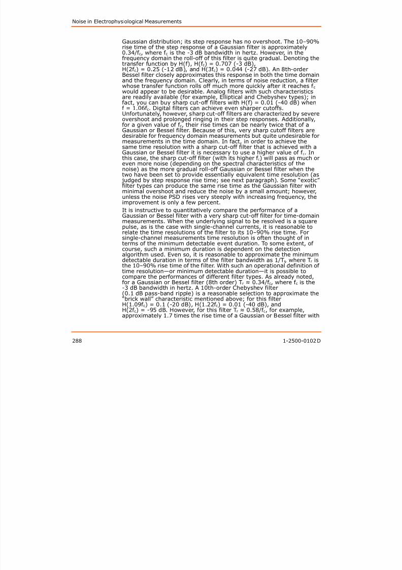
8/13/2019 User Guide v3
http://slidepdf.com/reader/full/user-guide-v3 289/302
288 1-2500-0102 D
/ r, r
the 10–90% rise time of the filter. With such an operational definition oftime resolution—or minimum detectable duration—it is possible tocompare the performances of different filter types. As already noted,for a Gaussian or Bessel filter (8th order) Tr ≈ 0.34/f c, where f c is the-3 dB bandwidth in hertz. A 10th-order Chebyshev filter(0.1 dB pass-band ripple) is a reasonable selection to approximate the
“brick wall” characteristic mentioned above; for this filterH(1.09f c) = 0.1 (-20 dB), H(1.22f c) = 0.01 (-40 dB), andH(2f c) = -95 dB. However, for this filter Tr ≈ 0.58/f c, for example,approximately 1.7 times the rise time of a Gaussian or Bessel filter with
The Axon Guide to Electrophysiology and Biophysics Laboratory Techniques
the same f c. Moreover the step response is characterized by a peakovershoot of about 20% and sustained ringing which is noticeable up toabout 10/f c. In order to achieve the same 10–90% rise time with the10th-order Chebyshev filter that is achieved with a Gaussian or 8th-order Bessel filter, it is necessary to select the -3 dB bandwidth of theChebyshev filter to be about 1.7 times higher than the -3 dB bandwidthof the Gaussian or Bessel filter. For example, the rise time of aChebyshev filter with f c = 17 kHz will be approximately the same asthat of a Gaussian or Bessel filter with f c = 10 kHz; it should be noted
that the step response of the Chebyshev filter will ring severely. Even ifthe ringing of its step and impulse response is ignored so that it isassumed that the 10th-order Chebyshev filter and the Gaussian orBessel filter have the same time resolution provided that f c (Chebyshev) ≈ 1.7f c (Gaussian), it is found that the Gaussian or Besselfilter significantly out-performs the Chebyshev filter in terms of noise inthe filtered signal.
For white noise it would be found that the Chebyshev filter would passapproximately 1.3x the noise passed by the Gaussian or Bessel filter,
provided, of course, that both filters had the same 10–90% rise time.For noise with a PSD that rises as f 2, the Chebyshev filter would actuallypass about 1.5x the rms noise passed by the Gaussian or Bessel filter,again provided that the filters’ corner frequencies were set to producethe same rise time. Obviously, when time resolution is considered,extremely sharp cut-off filters are not the best selection. Sharp cut-offfilters should only be used when frequency domain data (for example,power spectral density) is being collected.
Finally, as an illustration of the distinction between the -3 dB bandwidth
and the uppermost frequency component of noise that can passthrough a Gaussian or Bessel filter, consider a noise process (e2(f))whose PSD (V2 /Hz) rises as f 2 with increasing frequency. On linearscales such noise is shown in Figure 11-6 along with the transferfunction of a Gaussian filter (squared, H2(f)) and the noise PSD that willbe observed at the filter output (for example, H2(f)e2(f)). The squareroot of the integral of the filtered noise PSD (for example, the squareroot of the area under the curve) will be the rms noise. The PSD of thefiltered noise does not fall sharply at f c. In fact, the filtered PSD reaches
its peak at about 1.2 f c and does not fall to negligible levels until morethan 3 f c. This must be remembered when selecting a digitizing rate forany particular -3 dB filter setting if aliasing is to be avoided. Incomparison with a filter with a “brick wall” roll-off at the same fc the
8/13/2019 User Guide v3
http://slidepdf.com/reader/full/user-guide-v3 290/302
1-2500-0102 D 289
comparison with a filter with a brick wall roll off at the same f c, theGaussian filter will have somewhat more than 40% more noise at itsoutput. But recall that the sharp cutoff filter will have a much poorertime-domain response. In fact, as described above, if the -3 dBbandwidth of the sharp cut-off filter is selected to produce essentiallythe same time resolution as the Gaussian or Bessel filter, it will passeven more noise in this situation.
Noise in Electrophysiological Measurements
Figure 11-6 Squared transfer function of a Gaussian filter.
Illustrated are squared transfer function of a Gaussian filter (H2(f)),noise process with PSD that arises as f 2 with increasing frequency(e2(f)), and the same noise process PSD after passing through the
Gaussian filter (e2(f)H2(f)). The scales are linear; frequency isnormalized to the -3 dB bandwidth (f c) of the filter; PSD scale isarbitrary. Note that due to the gradual roll-off of the Gaussian filter, thefilt d i till h i ifi t ll b d f

8/13/2019 User Guide v3
http://slidepdf.com/reader/full/user-guide-v3 291/302
290 1-2500-0102 D
filtered noise still has significant power well beyond f c.
A useful alternative to adjusting the analog filter bandwidth to attemptto achieve an optimum signal-to-noise ratio is to digitize the data at arapid rate through a Bessel filter with its -3 dB bandwidth set toprevent aliasing. The wideband digitized data may then be filtereddigitally to achieve an acceptable signal to noise level. The digital filter
should once again generally be of the Gaussian or Bessel type. In suchsituations more than one filter are used in series; if these are all of the
The Axon Guide to Electrophysiology and Biophysics Laboratory Techniques
Gaussian or Bessel type, then the final -3 dB bandwidth, f cF, isapproximately given by:
where f 1, f 2, f 3 ... are the -3 dB bandwidths of the individual filters in
series. Of course, the same expression holds for a series combination ofanalog filters. The disadvantage to this general approach is that initialdata storage will be increased due to the high digitization rate; once thedata has been digitally filtered it can also be decimated if desired.
Summary of Patch-Clamp Noise
Headstage
At the time of publishing this guide, the best capacitive-feedbackheadstage (the CV 203BU of the Axopatch 200B amplifier) has anopen-circuit noise of about 0.13 pA rms in a 10 kHz bandwidth (-3 dB,8-pole Bessel filter). Resistive-feedback headstages have noise of about0.25–0.30 pA rms in this bandwidth. It is possible that developingcapacitive-feedback technology could yield further improvements innoise. In fact, in theory, it should be possible to produce acapacitive-feedback headstage with noise that is only about half of thatachieved presently.
Holder
The pipette holder contributes noise by increasing the capacitance atthe headstage input; some dielectric noise must also be expected. Theunshielded polycarbonate holders provided by Molecular Devices bythemselves will only increase the headstage noise by about 10% aboveits open circuit value even for the lowest noise capacitive-feedbackdevices. For example, for the Axopatch 200B amplifier with an
open-circuit noise of 0.060 pA rms in a 5 kHz bandwidth (as shown onthe panel meter), the total noise with the holder attached should notincrease beyond 0.070 pA rms (note that larger noise incrementsprobably mean that the holder needs to be cleaned) and will often be
8/13/2019 User Guide v3
http://slidepdf.com/reader/full/user-guide-v3 292/302
1-2500-0102 D 291
probably mean that the holder needs to be cleaned), and will often beas low as 0.065 pA rms. Inserting a saline-filled electrode into theholder will further increase noise even while the electrode tip is in air.With a saline-filled electrode, the noise of the Axopatch 200B with anopen-circuit noise of 0.060 pA in a 5 kHz bandwidth will generallyincrease to about 0.075 pA rms.
Noise in Electrophysiological Measurements
Electrode
The noise associated with the patch pipette is determined by the typeof glass used, the wall thickness of the glass, the pipette geometry, theuse of Sylgard coating, and the depth of immersion into the bath.Dielectric noise is probably the dominant source of noise associatedwith the electrode for all glasses except quartz. For glasses with lowerDε products—most notably quartz—it can be expected to become amuch smaller component of overall noise. Additional noise will arise
from the distributed resistance and capacitance of the pipette. For thebest glasses presently in common use, this source of noise is probablysomewhat less than the dielectric noise of the glass; for very low-lossglasses, such as quartz, it could be the dominant source of pipettenoise. A small amount of noise will also result from the thermal noise ofthe pipette resistance in series with the patch capacitance; only undercertain situations (a large patch area) will this “Re-Cp” noise becomesignificant.
Theoretical and experimental results indicate that a pipette fabricated
from the lowest-noise glasses (other than quartz) used to date(Corning #7760, #8161) with a moderate coating of Sylgard willproduce noise of about 0.2 pA rms in a 10 kHz bandwidth (8-poleBessel filter) for an immersion depth of about 2 mm. Under favorablecircumstances, this value can be cut at least in half when the tip of thepipette is withdrawn to within 100–200 μm of the surface of the bath.For pipettes fabricated from quartz, preliminary results indicate that fora 1 mm depth of immersion, noise of somewhat less than 0.1 pA rmscan be expected in a bandwidth of 10 kHz; with the very smallimmersion depth possible (10 μm or less) with the Silicone-fluidtechnique described above, it can be estimated that the noisecontributed by a quartz pipette falls to less than half of this value.Results obtained for quartz have involved pipettes with relatively longnarrow shanks and resistances of roughly 10 MΩ. Such a geometry isnot ideal for achieving the lowest possible noise. As techniques forpulling quartz pipettes improve, and as other grades and suppliers ofquartz are investigated, further improvements are likely.
Seal
The noise associated with the seal is less easily predicted. Certainly aminimum estimate of this noise in a bandwidth B is given by(4kTB/Rsh)1/2 for example the thermal current noise of the DC seal

8/13/2019 User Guide v3
http://slidepdf.com/reader/full/user-guide-v3 293/302
292 1-2500-0102 D
(4kTB/Rsh)1/2, for example, the thermal current noise of the DC sealresistance, Rsh. For excellent seals in the range of 50–200 GΩ thiswould mean that the minimum noise attributable to the seal is in therange of 0.03–0.06 pA rms in a 10 kHz bandwidth. Recent datasuggests that under favorable circumstances seal noise may be as lowas these predicted values. However, experience indicates that there is a
good deal of variability in the noise of patches even when the sealresistances are very high and all other precautions necessary to
The Axon Guide to Electrophysiology and Biophysics Laboratory Techniques
minimize noise have been strictly observed. Some of this variabilitymay well arise from the seal.
Limits of Patch-Clamp Noise Performance
A capacitive-feedback headstage, such as the CV 203BU of theAxopatch 200B amplifier, has an open circuit noise of less than 0.13 pArms in a 10 kHz bandwidth, (bandwidths are the -3 dB frequency of an
8-pole Bessel filter). The total noise is due to contributions from theheadstage, holder, pipette, and seal. However, peltier cooling hasremoved the thermal noise from this headstage, reducing total noisefrom 0.16 to about 0.13–0.14 pA rms in a 10 kHz bandwidth. Ofcourse, the noise associated with the seal is a fundamental limitation ofthe patch clamp technique. An absolute minimum estimate for sealnoise in a 10 kHz bandwidth is about 0.03–0.04 pA rms; this assumes a100–200 GΩ seal producing only thermal noise. An estimate of theminimum noise associated with an improved holder, quartz pipette and
seal in a 10 kHz bandwidth is then about 0.06 pA rms. These figuressuggest that as holder and pipette technology continues to improve, itwill be worthwhile to continue to seek methods to reduce the noise ofthe headstage itself. It is reasonable to expect that total noise levelsroughly two thirds of the best values achieved to date will becomepossible. However, to achieve such noise levels, careful attention toevery aspect of the patch-clamp technique will be important.
Further Reading
Rae, J.L., Levis, R.A., A method for exceptionally low noise single-channel recording. Pflugers Arch. 420, 618–620, 1992.
Rae, J.L., Levis, R.A., Quartz pipettes for single-channel recording.Biophys. 64, A201 (P394), 1993.
Sakmann, B. and Neher, E., Eds. Single-Channel Recording. New York:Plenum Press, 1983.

8/13/2019 User Guide v3
http://slidepdf.com/reader/full/user-guide-v3 294/302
1-2500-0102 D 293
Noise in Electrophysiological Measurements

8/13/2019 User Guide v3
http://slidepdf.com/reader/full/user-guide-v3 295/302
294 1-2500-0102 D
AGuide to Interpreting Specifications
General
Following are terms commonly used in electrophysiological
measurements.
Thermal Noise
All resistors generate thermal noise. Thermal noise can be representedby a mean square voltage generator (e2n) in series with a noiselessresistor:
where k = Boltzmann’s constant (1.138 x 10⁻²³ VC/°K)
T = temperature in °K
R = resistor value in ohms
B = bandwidth in Hertz
The noise specified by this equation has a constant power spectraldensity within the bandwidth and is zero outside the bandwidth. Whennoise is measured through a low-pass filter having -3 dB bandwidth f -3,
the noise will be greater than the amount predicted because real filterscontinue to pass signals at frequencies > f -3.
The noise of a 10 MΩ resistor measured through various filters isshown in Table A-1.
Table A-1 Noise of a 10 MΩ Resistor in Microvolts rms.
Bandwidth 1-Pole RC2-Pole
Butterworth4-Pole
ButterworthInfinitely
Sharp
DC-100 Hz 5.07 4.27 4.11 4.06
DC-1 kHz 16.0 13.5 13.0 12.8
DC-10 kHz 50.7 42.8 41.1 40.6

8/13/2019 User Guide v3
http://slidepdf.com/reader/full/user-guide-v3 296/302
1-2500-0102 D 295
DC 10 kHz 50.7 42.8 41.1 40.6
DC-100 kHz 160 135 130 128
Guide to Interpreting Specifications
RMS Versus Peak-to-Peak Noise
It is equally valid to specify noise as rms (root mean square) orpeak-to-peak. The ratio of the zero-to-peak value to the rms value iscalled the crest factor. The value of the crest factor depends on the typeof noise. For white noise the crest factor is about 4. Thus thepeak-to-peak noise is about 8 times the rms noise.
Bandwidth—Time Constant—Rise TimeFor an exponential response, there are simple relationships betweenthe -3 dB bandwidth (f -3, Hertz), the time constant (τ, seconds) andthe 10–90% rise time (t10–90; seconds):
Filters
Low-pass filters are commonly used in electrophysiology to reducenoise. The important parameters of a low-pass filter are the -3 dB
frequency, the type and the order.The -3 dB frequency (f -3) is the frequency where the voltage responsefalls to √ 2 (0.707). Some manufacturers specify the “cutoff ” or “bandwidth” based on the phase response or an asymptoticapproximation to the high and low frequency amplitude response.Therefore when using a new filter you should check that the specifiedsettings refer to the -3 dB frequency.
The three types of low-pass filters commonly used in electrophysiologyare the Bessel, Butterworth, and multiple coincident pole (RC) types.The most important differences are:
1. When driven by a step voltage, the RC filter has no overshoot,the Bessel filter has < 1% overshoot and the Butterworth filterhas around 10% overshoot

8/13/2019 User Guide v3
http://slidepdf.com/reader/full/user-guide-v3 297/302
296 1-2500-0102 D
has around 10% overshoot.
2. When driven by a noisy source, RC filters show the leastrejection of the noise at frequencies above f -3, Bessel filtersshow moderate rejection and Butterworth filters show the most.
The order of a filter refers to the number of poles. Each
resistor-capacitor section contributes one pole (inductors are rarelyused for bandwidths < 100 kHz). Thus 4th-order, 4-pole, and 4 RCsections all refer to the same thing.
The Axon Guide to Electrophysiology and Biophysics Laboratory Techniques
The attenuation of high-frequency noise increases with order. Atfrequencies well above f -3, the attenuation increases at 20 dB/decade(6 dB/octave) for each pole. Thus a 4-pole filter rolls off at80 dB/decade.
Microelectrode Amplifiers
Noise magnitude is very sensitive to the measurement technique.Specifications should state:
1. -3 dB bandwidth and order of the filter used in themeasurement circuit. Typically the noise will look 20–30% betterif a fourth-order low-pass filter is used instead of a first-order
low-pass filter.2. Microelectrode bandwidth. The capacitance neutralization should
be adjusted so that the -3 dB bandwidth of the microelectrode isthe same as the -3 dB bandwidth of the measurement circuit.
Voltage-Clamp Noise
Almost impossible to specify. Depends on cell mode, electrode model,capacitance neutralization setting, electrode interactions, electroderesistances, current measurement techniques, bandwidth ofmeasurement circuit and clamp gain.
10–90% Rise Time (t10–90)
The time for the response to go from 10% to 90% of the final value.
If a voltage step is applied to a microelectrode headstage via a resistor,the resistor should have a very low stray capacitance. Otherwise thestray capacitance couples the step directly into the headstage input andartificially fast rise times are measured. A better estimate of the risetime can be made by passing a current step out of the headstage into aload resistor.
For consistent comparisons, rise times should be measured with thecapacitance neutralization adjusted for zero overshoot
Note: 20 dB attenuation corresponds to a drop in voltage amplitudeto one tenth.

8/13/2019 User Guide v3
http://slidepdf.com/reader/full/user-guide-v3 298/302
1-2500-0102 D 297
capacitance neutralization adjusted for zero overshoot.
1% Settling Time (t1)
When microelectrodes are to be used in a discontinuous (switching)single-electrode voltage clamp, the more relevant specification is t1, the
time taken for the response to go from 0% to 99% of the final value.
Guide to Interpreting Specifications
Input Capacitance
In a circuit using capacitance neutralization and other compensationtechniques, it is meaningless to specify a value for the inputcapacitance. The efficacy of the neutralization circuit depends on themagnitude of the electrode resistance and the measurement technique.
For an electrode with resistance R and an exponential response to astep input, the effective input capacitance can be estimated from:
For example, if t10-90 = 10 μs and R = 10 MΩ, then Cin = 0.45 pF.
Input Leakage Current
Both well designed and badly designed headstages are normallyadjustable to zero leakage current. This ability in itself is not animportant test of quality. The correct measure of quality is thesensitivity of the input leakage current to temperature changes whichoccur after the adjustment is made. Changes of ±10°C can beexpected in a typical laboratory environment.
Patch-Clamp Amplifiers
BandwidthThe bandwidth of a patch-clamp headstage is usually measured byinjecting current into the headstage input through a small capacitor. Noholder or electrode is attached to the input.
The bandwidth during an experiment is usually much lower. It istypically limited by the electrode resistance and membranecapacitance, as well as by stray capacitances. For example, if a 5 MΩelectrode is used to clamp a whole cell having 20 pF of membranecapacitance, the time constant for measuring membrane currents is100 μs (5 MΩ x 20 pF). This corresponds to a -3 dB bandwidth of1.6 kHz, far below the 100 kHz that may be specified. 80%series-resistance compensation would improve this to 8 kHz.Nevertheless, it is still better to have a headstage with very wide

8/13/2019 User Guide v3
http://slidepdf.com/reader/full/user-guide-v3 299/302
298 1-2500-0102 D
, g ybandwidth because in some cases series-resistance compensation maywork better.
The Axon Guide to Electrophysiology and Biophysics Laboratory Techniques
Noise
The ideal RMS current noise in selected bandwidths is shown inTable A-2 for various feedback resistors. These figures assume idealresistors (which only have thermal noise) and noiseless electronics.
No patch-clamp amplifier can meet these ideal specifications. Thedifference between a value in the table and the actual value is theexcess noise. The excess noise is always proportionately worse in thewider bandwidths.
Table A-2 rms Current in Picoamps.
BANDWIDTH 500 MΩ 1 GΩ 5 GΩ 10 GΩ 50 GΩ
DC-1 kHz 0.182 0.128 0.057 0.041 0.018
DC-3 kHz 0.331 0.234 0.099 0.074 0.033
DC-10 kHz 0.574 0.406 0.181 0.128 0.057
Note: The specified noise in a 10 kHz bandwidth will be misleadinglylow if the headstage does not have a 10 kHz bandwidth. If themanufacturer only specifies the 10–90% rise time or the timeconstant, use the conversion factors given in the General section toverify that the bandwidth is sufficient to make the noise specificationmeaningful.

8/13/2019 User Guide v3
http://slidepdf.com/reader/full/user-guide-v3 300/302
1-2500-0102 D 299
Guide to Interpreting Specifications

8/13/2019 User Guide v3
http://slidepdf.com/reader/full/user-guide-v3 301/302
300 1-2500-0102 D

8/13/2019 User Guide v3
http://slidepdf.com/reader/full/user-guide-v3 302/302
FOR RESEARCH USE ONLY. NOT FOR USE IN DIAGNOSTIC PROCEDURES. The trademarks mentioned herein are the property of Molecular Devices, LLC or their respective owners. ©2012 Molecular Devices, LLC.
Contact UsPhone: +1-800-635-5577
Web: www.MolecularDevices.comEmail: [email protected] our web site for a current listing of
worldwide distributors.
Regional OfficesUSA and Canada +1-800-635-5577
Brazil +55-11-3616-6607
China (Beijing) +86-10-6410-8669
China (Shanghai) +86-21-3372-1088
Germany +49-89/96-05-88-0
Japan (Osaka) +81-6-7174-8831
Japan (Tokyo) +81-3-6362-5260
South Korea +82-2-3471-9531
United Kingdom +44-118-944-8000