International Conference on Climate Change and Water (THA 2015)

WARDAH TAHIR, SAHOL HAMID ABU BAKAR

SUZANA RAMLI, SH HUDA SY YAHYA AND AHMAD KAMIL AMINUDDIN, MARFIAH ABD WAHID

Flood Control Research Center Faculty of Civil Engineering Universiti Teknologi MARA

MALAYSIA.

Use of Multi-sensors Data Input for

Improved Flood Forecasting

Global Warming and Climate Change The Intergovernmental Panel on Climate Change (IPCC) Third Assessment Report (2001) and Fourth Assessment Report (2007) predicted impacts from the global warming

More floods: from both increased heavy precipitation events and sea level rise. Increased spread of infectious diseases. Degraded water quality: higher water temperatures will tend to degrade water quality and increased pollutant load from runoff and overflows of waste facilities. More frequent and more intense heat waves, droughts, and tropical cyclones

Source: IPCC Report, 2007

Factor Affecting Increase in Flood Disasters

Global warming- glacier melting causing sea level rise

http://i186.photobucket.com/albums/x70/AnthonyMarr/glacier-melting1941-2008-1.jpg

Muir Glacier in Alaska 1941 vs 2006

Swiss Glacier 1909 vs 2004

Flood in Malaysia – December 2014

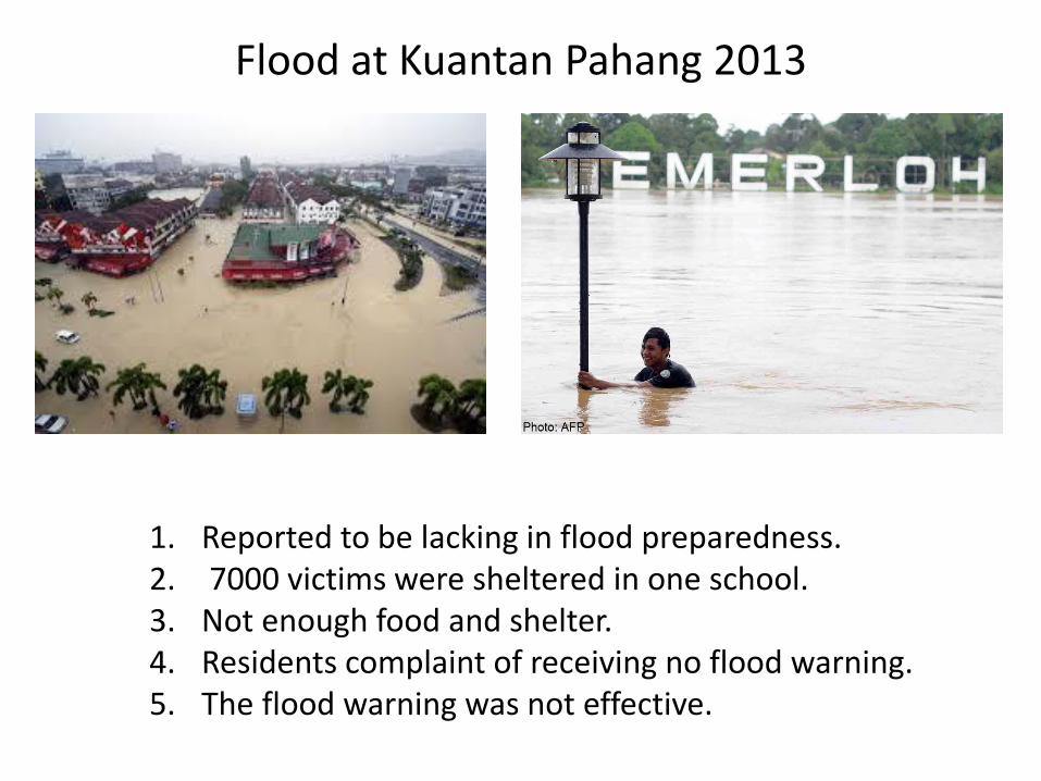
Flood at Kuantan Pahang 2013

1. Reported to be lacking in flood preparedness. 2. 7000 victims were sheltered in one school. 3. Not enough food and shelter. 4. Residents complaint of receiving no flood warning. 5. The flood warning was not effective.

Flood forecasting and warning

Flood forecasting and warning can provide longer lead times for immediate actions by the authority or the community. However, early warning is effective if only people understand the language of early warning and be able to respond appropriately.

USE OF MULTISENSOR DATA INPUT FOR IMPROVED FLOOD FORECASTING

• Use of Geostationary Meteorological Satellite

• Use of Radar

• Use of Numerical Weather Prediction

7

USE OF GEOSTATIONARY METEOROLOGICAL SATELLITE INFRARED IMAGES

FOR CONVECTIVE RAINFALL ESTIMATES

Geostationary meteorological

satellites have fixed position.

The satellites make observations

at 20-30 minute intervals

throughout each day over the

same area, therefore able to

monitor the raining cloud cell

development over an area, thus

forecast intense storm causing

flood

Source: USA Today

Convective rain occurs when heated air is rising and cooled until the condensation occurs and cloud droplets grows then become large enough to fall as rain. The higher the air parcel rise, the colder the cloud temperature.

Hence, it is assumed that cloudy satellite image pixels colder than a given threshold temperature are associated with probably precipitating cumulonimbus clouds.

HOW CLOUD TOP BRIGHTNESS TEMPERATURE FROM THE INFRARED IMAGES ARE RELATED WITH CONVECTIVE RAIN

April 11, 2003 (Stn 3217002)

0

10

20

30

40

50

60

70

1 2 3 4 5 6 7 8 9

Time (hr)

Rain

Dep

th (

mm

)

180

200

220

240

260

280

300

Clo

ud

To

p

Tem

pera

ture

(K

)

Rain Temp

Closest pixel to

Station 3116003

Programming/ image processing using Matlab to

determine station pixel intensity value

Use McIDAS-V software to read cloud top brightness temperature

Development of Satellite Based Rainfall Estimations using Artificial Neural Network

Tall overshooting convective raining cloud indicated by sobel operator

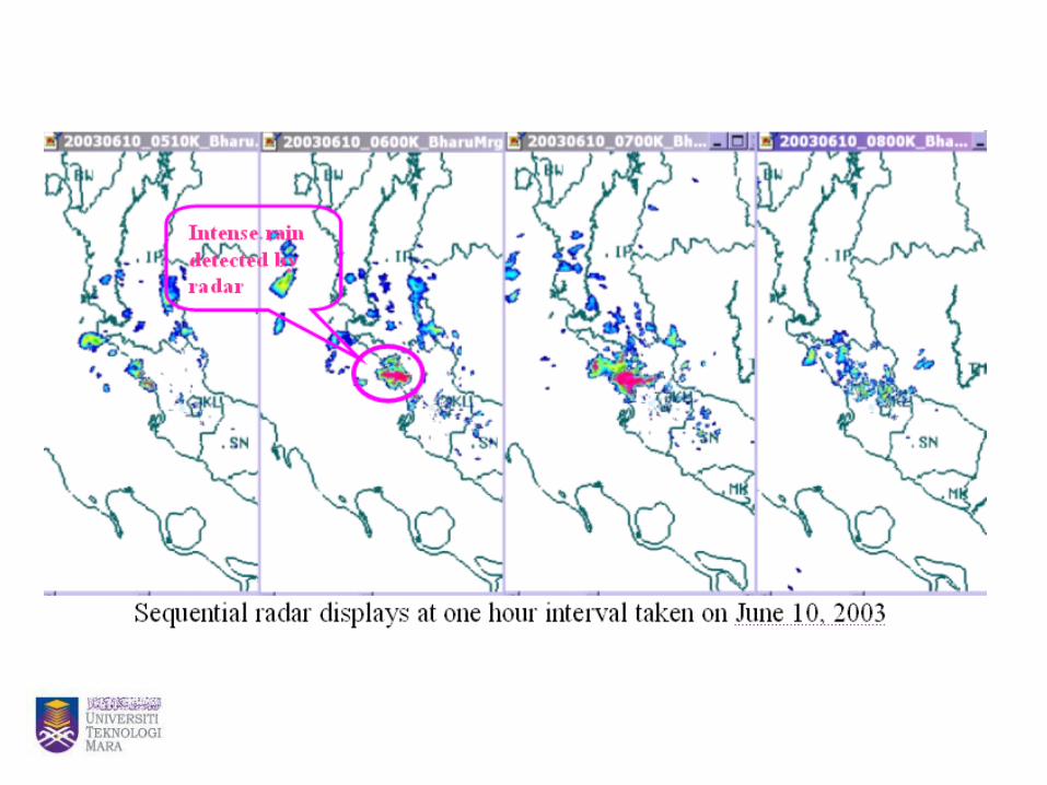
Rain Estimation over case study area of Upper Klang River Basin

( 4 pm, June 10, 2003 )

Example of June 10, 2003 (Flash Flood

Event) Rain Estimation

comparison using RainIRSat and

ANN-based techniques

Flash Flood Event : June 10, 2003

0

10

20

30

40

50

60

16 17 18 19 20 21 22 23 24 1 2 3

Time (hr)

Ra

infa

ll d

ep

th (

mm

)

0

100

200

300

400

500

600

Ru

no

ff (

m3/s

)

Thiessan

Average

Rain

RainIRSat

ANN

Recorded

flow

0.0

10.0

20.0

30.0

40.0

50.0

60.0

70.0

80.0

90.0

Jun_10 Jun_13 Jun_15 Jun_23 Jun_24 Jun_28

Are

al A

vera

ged

Rai

n(m

m).

RainIRSat Thiessan ANN

Hourly estimation of areal averaged rain depth for upper Klang River Basin on June 10, 2003 flash flood event.

Estimates of total areal averaged rain depth for upper Klang River Basin for several events

0.0 10.0 20.0 30.0

Thiessan (mm)

0.0

10.0

20.0

30.0

AN

N (

mm

)

95% mean prediction intervalr = 0.63

HOURLY RAINFALL ESTIMATION

Validation of ANN hourly areal averaged rainfall estimation against gauge measured Thiessen areal averaged rain (107 hourly rain from 33 storm

events from year 2006 )

10.0 20.0 30.0 40.0 50.0

Thiessan (mm)

10.0

20.0

30.0

40.0

50.0

60.0

AN

N (

mm

)

95% mean prediction intervalr=0.91

TOTAL RAINFALL ESTIMATION

Validation of ANN total areal averaged rainfall estimation against gauge measured Thiessen areal averaged rain (33 storm events from year 2006)

Rain-Watch offers four complementary rain estimation options. Users can easily estimate and forecast rainfall for their flood monitoring system or any rainfall-related

disaster monitoring system using the user-friendly graphical-user-interface Rain-Watch application

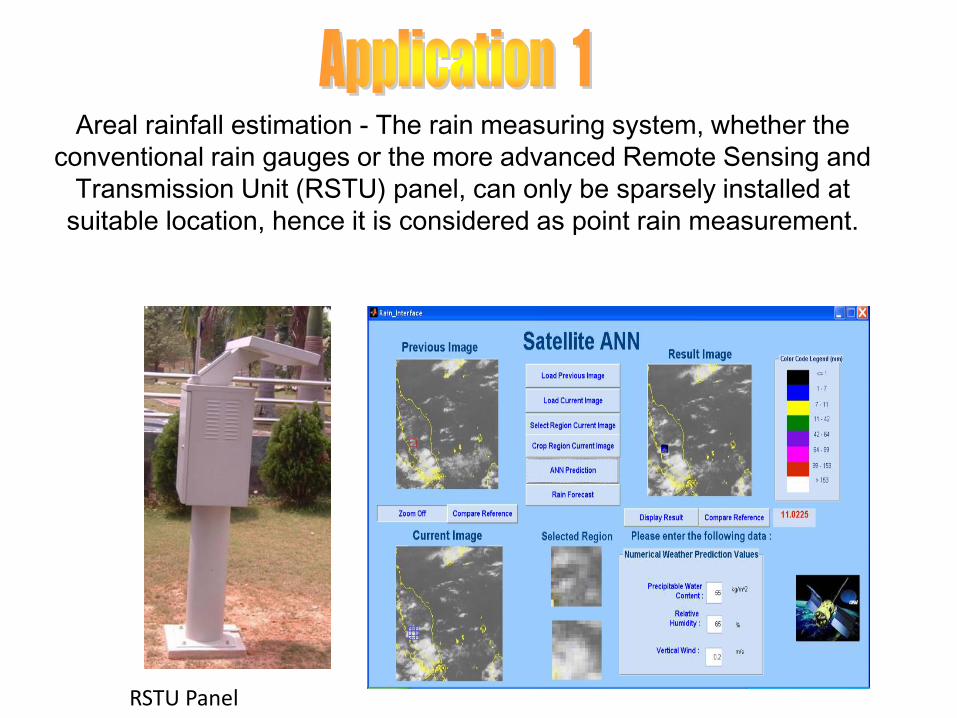
Areal rainfall estimation - The rain measuring system, whether the

conventional rain gauges or the more advanced Remote Sensing and

Transmission Unit (RSTU) panel, can only be sparsely installed at

suitable location, hence it is considered as point rain measurement.

RSTU Panel

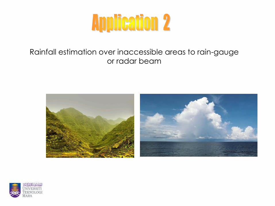
Rainfall estimation over inaccessible areas to rain-gauge or radar beam

A coupled hydro-meteorological flood forecasting system.

Flash flood forecasting for an improved lead time of flood warning

Cross-correlation option in Rain-Watch for rainfall forecast

EARLY FLOOD WARNING WOULD ALLOW ENOUGH TIME

TO SAVE PROPERTIES

Catchment with short response times requires improved flood forecasting technique. By coupling meteorological and the hydrological model the lead time between

occurrence of a storm event and flood warning can be extended.

CROSS CORRELATION TECHNIQUE TO TRACK THE DIRECTION OF CLOUD MOVEMENT

(Rogers and Yau, 1996)

Schematic view of a multi-cell storm

Max r value

Storm Event : June 10, 2003 (Flash Flood Event)

0

5

10

15

20

25

30

35

40

12 13 14 15 16 17 18 19 20 21 22 23 24 1 2 3

Time (hr)

Ra

infa

ll d

ep

th (

mm

)

0.0

100.0

200.0

300.0

400.0

500.0

600.0

Ru

no

ff (

m3/s

)

ANN Forecast Rain Forecasted flow Recorded Flow

New lead time

0.0

5.0

10.0

15.0

20.0

25.0

30.0

35.0

0.0

10.0

20.0

30.0

40.0

50.0

60.0

Hour_15 Hour_16 Hour_17 Hour_18 Hour_19

Alb

edo (

%)

Ran

ifall

(m

m)

Time (UTC)

Rainfall (mm) Albedo (%)

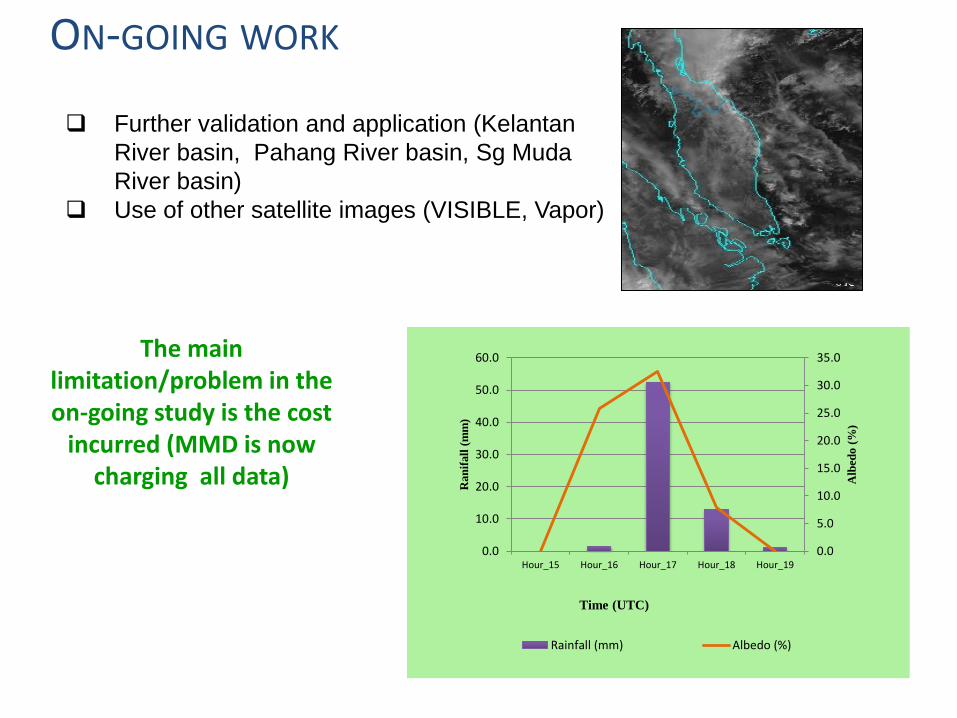
ON-GOING WORK

Further validation and application (Kelantan

River basin, Pahang River basin, Sg Muda

River basin)

Use of other satellite images (VISIBLE, Vapor)

The main limitation/problem in the on-going study is the cost

incurred (MMD is now charging all data)

RADAR

Radar stands for Radio Detection and Ranging.

It detects the position, velocity and characteristics of targets.

Weather radar sends directional pulse of microwave

The energy of each pulse will bounce off the small particles (droplets) back in the direction of the radar station.

The signal in reflectivity will then be converted into rain rate.

The relationship between reflectivity, Z and rainfall rate, R is established empirically and it is known as Z-R relationships

32 Source : Malaysian Meteorological Department

Doppler Radar

• Development of Doppler radar starts in the era of 1970s

• Doppler radar, which is situated in Bukit Tampoi, Dengkil, about 10 km to North KLIA was first introduced in 1998.

• The prime function of TDR is to detect and to alert KLIA on the wind shear problem and also microburst scenario. Both conventional and Doppler radars can detect rainfall intensity through its signal reflectivity.

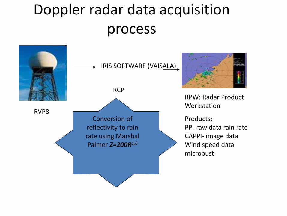
Doppler radar data acquisition process

IRIS SOFTWARE (VAISALA)

RVP8

RCP RPW: Radar Product Workstation

Conversion of reflectivity to rain rate using Marshal Palmer Z=200R1.6

Products: PPI-raw data rain rate CAPPI- image data Wind speed data microbust

An example of a Doppler radar image during a flash flood (June 10, 2007)

The use of radar in quantitative precipitation estimation (QPE)

Advantages

Disadvantages Less accuracy due to several errors (as follows): Z-R variability Ground clutter contamination Bright band effects Beam attenuation Vertical profile reflectivity Rain gauge representativeness Miscellaneous (poor maintenance and radar

calibration)

High resolution in temporal and spatial

OUR STUDY : IMPROVING Z/R Relationship

• Many studies had shown that with inappropriate use of Z/R relations, the rainfall estimates are proved to be inaccurate (Zogg, 2006).

R² = 0.6638

0

50

100

150

200

250

300

350

-10 10 30 50 70 90 110 130 150

Rad

ar R

ain

fall

(mm

/hr)

Gauged Rainfall (mm/hr)

The comparison between new and current Z-R relationship categorized

into monsoon and rain intensity

44

CATEGORY OF RAIN Z-R Equations Mean

Absolute

Error

LOW New Z=180R1.9 3.08

Current Z=200R1.6 4.58

MODERATE New Z=212R1.9 7.18

Current Z=200R1.6 15.86

HEAVY New Z=262R1.9 15.04

Current Z=200R1.6 67.48

SOUTHWEST

MONSOON

New Z=500R1.9 8.66

Current Z=200R1.6 56.25

NORTHEAST

MONSOON

New Z=166R1.9 13.03

Current Z=200R1.6 32.78

INTERSWM New Z=367R1.9 11.54

Current Z=200R1.6 99.44

INTERNEM New Z=260R1.9 32.04

Current Z=200R1.6 97.58

45

Flood hydrograph after an unsteady flow

analysis using different rainfall inputs

Gombak river basin model network

and radar rainfall input

APPLICATION OF RADAR RAINFALL INPUT

On-going work

• Further improvement in radar rainfall estimation, reducing error by Kalman filter

• Radar rainfall input into grid-based rainfall-runoff model

46

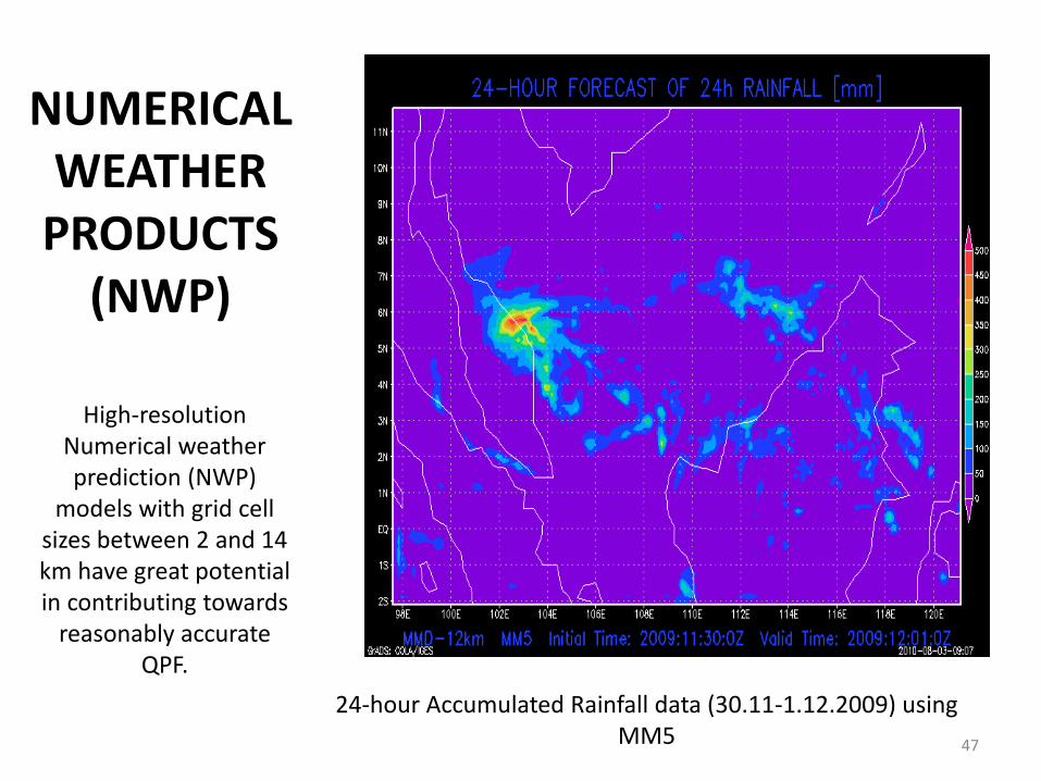
NUMERICAL WEATHER

PRODUCTS (NWP)

High-resolution Numerical weather prediction (NWP)

models with grid cell sizes between 2 and 14 km have great potential in contributing towards

reasonably accurate QPF.

47

24-hour Accumulated Rainfall data (30.11-1.12.2009) using MM5

What is

Numerical Weather Prediction (NWP) ?

Objective weather forecasts by solving a set of governing equations that describe the

evolution of the present state of the atmosphere (e.g: conservation of momentum,

conservation of mass, moisture, and gas law) . The process involves initial variables that

describes the current state of the atmosphere such as: humidity, temperature, wind

velocity, pressure. Fundamental equations of physics represent these variables and

through integration over time a forecast or an estimation of the variables at the future

state is made.

Example NWP equations:

48

During the 1970’s several NWP modelling systems

were implemented, global, hemispheric or as limited area models (LAMs).

LAMs ran with a higher resolution over a smaller area and took boundary conditions from a larger hemispheric or global model.

During the last decades, several regional LAMs have been developed such as the Fourth Generation Penn State/NCAR Mesoscale (MM4) and later the MM5 (Grell et al. 1994) and the new Weather Research and Forecasting (WRF) model (NCAR/UCAR, 2005).

Today, NWP is the most widely used prediction system, and can predict future states for up to 10 days.

49

NWP used by the Malaysian Meteorological Department

Malaysian Meteorological Department (MMD) currently uses the MM5 and the WRF for the weather forecasting purposes. NWP model outputs include forecasts for rainfall, humidity, wind speed and a range of other derived variables which may be useful for flood forecasting.

With advances in NWP in the recent years as well as an increase in computing power, it is now possible to generate very high resolution rainfall forecast at the catchment scale.

50

OUR STUDY :

Statistical verification of two NWP models namely MM5 and WRF against gauged rain over Kelantan River Basin and Klang River Basin.

Comparison of MM5 and WRF performance against gauged rain over Kelantan River Basin.

51

• Fifth Generation Penn State/NCAR Mesoscale (MM5)

• Weather Research and Forecasting (WRF)

52

Datasets used

Use software Grid Analysis and Display System (GrADS) for processing NWP data

Model runs at 00UTC (0800 local time) Forecast ranges are hourly, up to a period of 72 hours. 4 km resolution

NWP model used in Malaysia

Rainfall

Hourly rainfall at 9 gauged stations over Kelantan River basin (DID) for year 2009

53

The location of Kelantan River Basin on the WRF display.

54

55

Results

Though the model overestimates the 24-hr rainfall quite notably during Mac, April, May, August and September, they

follow almost similar pattern of the mean daily rainfall amount

56

Results – Root Mean Square Error (RMSE)

The longer forecast duration, the greater RMSE Comparison between the two models, indicate that their performance follow similar pattern

It is observed that WRF performed slightly better than MM5 especially for 24-hr forecast.

57

Results

RMSE for different categories of rainfall (light, moderate, heavy)

WRF MM5

58

Probability of Detection (POD) and False Alarm Ratio (FAR)

POD- fraction of observed events that were correctly forecasted FAR - fraction of forecast events that were observed to be nonevents

The longer rainfall forecast duration, the higher the POD and the lesser FAR

59

November 5 - 11 (areal average daily rainfall of 234 mm on 5th November) November 20 – 26 (areal average daily rainfall of 125 mm on 20th November)

December 2 – 6 (areal average daily rainfall of 139 mm on 2nd December)

Prediction of Rainfall causing Flood Events

For the first event, both models forecast well before the flood event, but miss the very heavy rainfall on November 5 During the second flood event, both models produce 24-hr forecast which are closed to the rainfall that had caused the flood with WRF performed slightly better. The third event indicates that the QPF produced by the WRF forecast is much closer than the overestimated value from the MM5

1

2

3

On-going work

• Further statistical verification

• Ensembles with weather satellite and radar rainfall estimation and forecasting.

60

Conclusion

61

Geostationary meteorological satellite,

radar and numerical weather prediction

model are very promising tools to be used

to improve our flood forecasting.

More work should be done; support and

collaborative work should be strengthened

for the technological advancement of our

nation

62

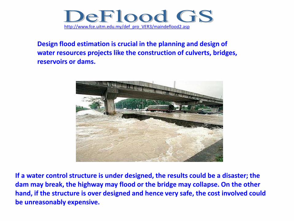
If a water control structure is under designed, the results could be a disaster; the dam may break, the highway may flood or the bridge may collapse. On the other hand, if the structure is over designed and hence very safe, the cost involved could be unreasonably expensive.

Design flood estimation is crucial in the planning and design of water resources projects like the construction of culverts, bridges, reservoirs or dams.

http://www.fce.uitm.edu.my/def_pro_VER3/maindeflood2.asp

Design Flood Estimation Guidance System Version 3.0 or DeFlood GS provides a convenient and fast approach to compute the design flood estimation values. The techniques implemented in

this application are Site Frequency Analysis, Rational Method, Regional Flood Frequency Analysis, Triangular Hydrograph Method and SCS Method

http://www.fce.uitm.edu.my/def_pro_VER3/maindeflood2.asp

Conclusion

Flooding as one of the most devastating natural hazards has affected millions of people throughout the

world. The implementation of various strategies and solutions to overcome the disasters depends on the

capabilities of the regions, the authorities involved and the commitment of the government. An integrated

flood management solution with participation from all stakeholders is crucial to ensure the effectiveness of the measures. At community level, all individuals can

contribute to flood disaster control by reducing vulnerabilities at their sites.