USE OF A WINDBREAKER TO MITIGATE HIGH SPEED WIND …

USE OF A WINDBREAKER TO MITIGATE HIGH SPEED

WIND LOADING ON A MODULAR DATA CENTER

by

PRASAD PRAMOD REVANKAR

Presented to the Faculty of the Graduate School of

The University of Texas at Arlington in Partial Fulfillment

of the Requirements

for the Degree of

MASTER OF SCIENCE IN MECHANICAL ENGINEERING

THE UNIVERSITY OF TEXAS AT ARLINGTON

May 2015

ii

Acknowledgements

I would like to take this opportunity to thank my supervising professor Dr.

Dereje Agonafer for his constant encouragement, support and guidance during the

course of my research and studies at this University. The invaluable advice and

support provided by him was the major driving force, which enabled me to

complete my thesis.

I would like to thank Dr. Kent Lawrence and Dr. Haji-Sheikh for taking

time to serve on my thesis committee. Also, I would like to thank Betsegaw

Gebrehiwot for his invaluable support and timely inputs.

I am obliged to Ms. Sally Thompson and Ms. Debi Barton for helping me

out in all educational matters. They have been very kind and supportive whenever

I needed their help.

I would like to thank all my friends in the EMNSPC team and in the

University for helping me throughout my time here at this University. Finally, I

would like to thank my parents for their support, both emotionally and financially,

without which I would not have been able to complete my degree.

April 21, 2015

iii

Abstract

USE OF A WINDBREAKER TO MITIGATE HIGH SPEED

WIND LOADING ON A MODULAR DATA CENTER

Prasad Pramod Revankar, MS

The University of Texas at Arlington, 2015

Supervising Professor: Dereje Agonafer

The data centers that are located in open regions are subjected to various

environmental risks such as floods and very strong winds. As this wind blows

over the data center, the pressure difference generated can have destructive effects

on the data center. Various kinds of fences have been used as windbreakers to

reduce the wind speed and divert the wind. A windbreaker basically acts as a

barrier to the upstream wind and reduces the mean velocity of air downstream of

the windbreaker, thereby reducing the wind loading on the objects situated behind

the fence. The height, width, and void volume fraction of the windbreaker are

main parameters that determine the level of wind speed reduction across the

windbreaker. The aim of this computational investigation is to design a

windbreaker for reducing sustained wind speed of 44.7 m/s (100 mph) to 9 m/s

(20 mph) average velocity in the direction normal to wall, at a distance of 0.3 m

(1 ft) from the wall of the modular data center (MDC).

iv

The model of the windbreaker and an enclosure of the modular data center

was created in FloTHERM 10.1. The windbreaker has a split wall configuration,

in which two windbreakers, one on the ground the other on the roof of the data

center, are used. Various parameters of the windbreaker such as height, void

volume fraction and distance from the MDC are varied to study how these

parameters affect the average normal-to-the-wall wind speed on a projected area

of the MDC. The combination of these parameters that satisfy the criterion

mentioned above are considered acceptable basic design parameters for the

windbreaker. It is observed that, with the use of these windbreakers, there is a

significant change in pressure that reduces the wind load induced damage. The

design enables the use of existing modular data centers without the need for

improving them to withstand high speed winds.

v

TABLE OF CONTENTS

Acknowledgements ................................................................................................. ii

Abstract .................................................................................................................. iii

List of Illustrations ............................................................................................... viii

List of Tables ......................................................................................................... ix

Chapter 1 INTRODUCTION .................................................................................. 1

1.1 Modular Data Centers ................................................................................... 3

1.1.1 An Introduction ...................................................................................... 3

1.1.2 Yahoo’s Chicken Coop Data Center ...................................................... 5

Chapter 2 WINDBREAKERS ................................................................................ 8

2.1 Effectiveness of the Windbreak .................................................................. 10

2.1.1 Effect of Height .................................................................................... 10

2.1.2 Effect of Distance................................................................................. 11

2.1.3 Effect of Density .................................................................................. 11

2.1.4 Effect of Orientation ............................................................................ 13

2.1.5 Effect of Length ................................................................................... 14

Chapter 3 COMPUTATIONAL FLUID DYNAMICS (CFD)

ANALYSIS ........................................................................................................... 15

3.1 Introduction to CFD Analysis ..................................................................... 15

3.2 Governing Equations .................................................................................. 16

3.3 Turbulence Modeling .................................................................................. 19

vi

3.3.1 LVEL Turbulence Model ..................................................................... 19

3.3.2 K-Epsilon Turbulence Model .............................................................. 19

3.4 Meshing and Grid Constants ....................................................................... 20

3.5 Smart Parts in FloTHERM 10.1 ................................................................. 21

3.5.1 Cuboid .................................................................................................. 21

3.5.2 Resistance ............................................................................................ 21

3.5.3 Enclosure .............................................................................................. 22

3.5.4 Source .................................................................................................. 22

3.5.5 Monitor Points ..................................................................................... 22

3.5.6 Region .................................................................................................. 23

3.5.7 Command Center ................................................................................. 23

Chapter 4 DESCRIPTION OF THE MODEL ...................................................... 25

4.1 Description of the Modular Data Center ..................................................... 25

4.2 Description of the Windbreaker .................................................................. 26

4.3 Description of the CFD Model ................................................................... 27

4.3.1 Dimensions of the Model ..................................................................... 27

4.3.2 Model Setup ......................................................................................... 27

4.3.3 Boundary conditions ............................................................................ 28

4.3.4 Meshing ................................................................................................ 29

4.4 Mesh Sensitivity Analysis .......................................................................... 29

4.5 Scenarios Considered .................................................................................. 31

vii

Chapter 5 RESULTS AND CONCLUSION ........................................................ 32

5.1 For 5% void volume fraction ...................................................................... 32

5.1.1 Velocity profile at 0.5m from MDC .................................................... 33

5.1.2 Velocity profile at 2m from MDC ....................................................... 34

5.1.3 Velocity profile at 3.5m from MDC ..................................................... 35

5.2 For 10% void volume fraction .................................................................... 37

5.3 For 20% void volume fraction. ................................................................... 38

5.4 For 30% void volume fraction .................................................................... 39

5.5 For 40% void volume fraction. ................................................................... 40

5.6 Plot of Normalized Speed vs Windbreaker distance .................................. 40

5.6 Conclusion .................................................................................................. 41

Chapter 6 SCOPE AND FUTURE WORK .......................................................... 43

References ............................................................................................................. 44

Biographical Information ...................................................................................... 45

viii

List of Illustrations

Figure 1 Dell EPIC Modular Data Center for eBay [4] .......................................... 4

Figure 2 Yahoo Compute Coop Data Center facility[5] ......................................... 7

Figure 3 Windbreakers used at airports .................................................................. 9

Figure 4 Wind sped behind a windbreaker as percentage of incoming speed ........ 9

Figure 5 Effect of density ..................................................................................... 12

Figure 6 Representation of a 3D grid .................................................................... 18

Figure 7 3D model of MDC .................................................................................. 26

Figure 8 Split Wall configuration schematic ........................................................ 27

Figure 9 Mesh of the CFD model ......................................................................... 29

Figure 10 Mesh Sensitivity Analysis .................................................................... 30

Figure 11 Half-model with boundary conditions .................................................. 31

Figure 12 Lower wall at 0.5m from MDC ............................................................ 33

Figure 13 Upper wall at 0.5m from MDC ............................................................ 34

Figure 14 Lower wall at 2m from MDC ............................................................... 34

Figure 15 Upper wall at 2m from MDC ............................................................... 35

Figure 16 Lower wall at 3.5m from MDC ............................................................ 35

Figure 17 Upper wall at 3.5m from MDC ............................................................ 36

Figure 18 Particle track for 5% void volume fraction of windbreaker ................. 36

Figure 19 Particle track for 20% void volume fraction of windbreaker ............... 39

Figure 20 Graph of normalized speed vs windbreaker distance from MDC ........ 41

ix

List of Tables

Table 1 Saffir-Simpson Hurricane wind scale ........................................................ 2

Table 2 Dimensions of the model ......................................................................... 27

Table 3 Mesh Sensitivity analysis......................................................................... 30

Table 4 5% void volume fraction.......................................................................... 32

Table 5 10% void volume fraction ........................................................................ 37




1

Chapter 1

INTRODUCTION

Data Centers are a facility which store computer systems and other

components, like data storage units, telecommunication systems, etc. The

equipment in these data centers requires a certain controlled environment for its

optimum functionality. This requires an efficient cooling system as well, since the

huge amount of IT equipment within the data center produces a large amount of

heat. So, the entire data center is an expensive facility that needs to be maintained

and protected from any sort of damage or factors that would cause

malfunctioning.

One of the major issues taken into consideration while designing a data

center, is the environmental effects on the external structure. Earthquakes have

the greatest effect on the structural integrity of a data center followed by wind

loading. Strong, high speed winds can cause significant damage to the external

structure or claddding of the data center. As the wind blows against the external

structure, there is a build up of pressure against the external structure which is

translated to the supporting structure. Also as the wind blows over the structure, it

can generate an upward force on the roof. It can lead to localized damage to the

roof, cladding or the support structure. In case of very high speed winds, which

are caused by hurricanes or tornadoes, the wind loading can lead to lateral

deformation of the structure.

2

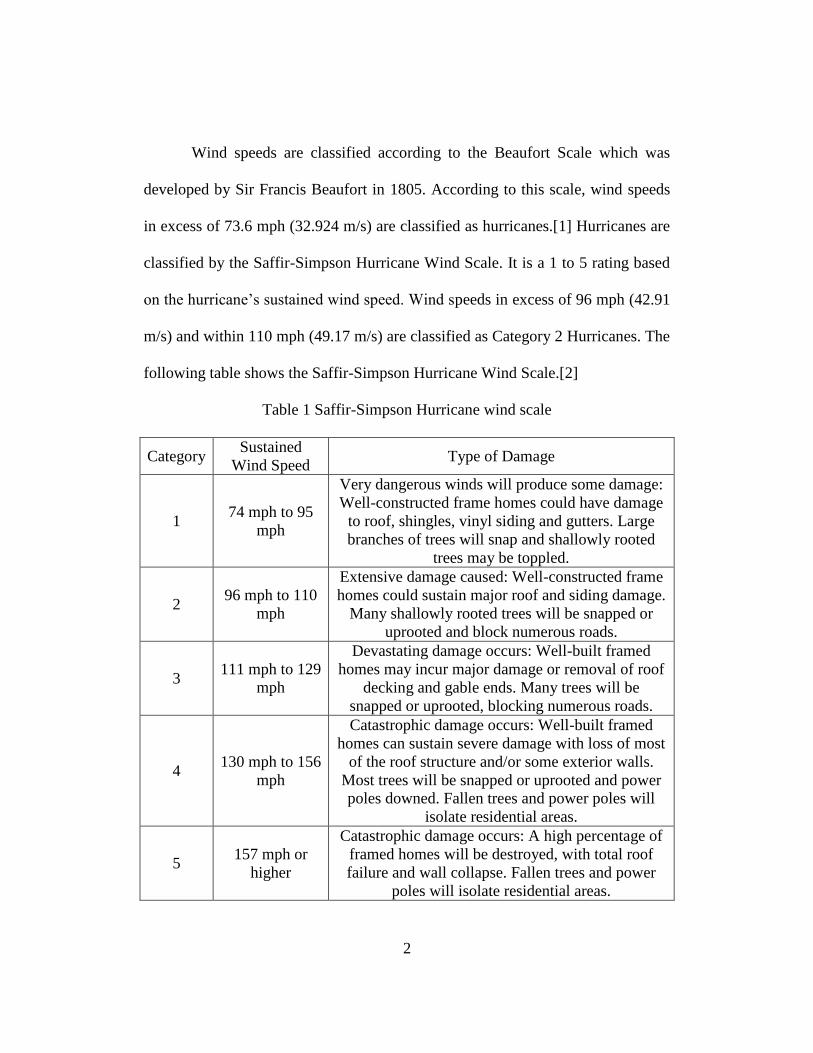
Wind speeds are classified according to the Beaufort Scale which was

developed by Sir Francis Beaufort in 1805. According to this scale, wind speeds

in excess of 73.6 mph (32.924 m/s) are classified as hurricanes.[1] Hurricanes are

classified by the Saffir-Simpson Hurricane Wind Scale. It is a 1 to 5 rating based

on the hurricane’s sustained wind speed. Wind speeds in excess of 96 mph (42.91

m/s) and within 110 mph (49.17 m/s) are classified as Category 2 Hurricanes. The

following table shows the Saffir-Simpson Hurricane Wind Scale.[2]

Table 1 Saffir-Simpson Hurricane wind scale

Category Sustained

Wind Speed Type of Damage

1 74 mph to 95

mph

Very dangerous winds will produce some damage:

Well-constructed frame homes could have damage

to roof, shingles, vinyl siding and gutters. Large

branches of trees will snap and shallowly rooted

trees may be toppled.

2 96 mph to 110

mph

Extensive damage caused: Well-constructed frame

homes could sustain major roof and siding damage.

Many shallowly rooted trees will be snapped or

uprooted and block numerous roads.

3 111 mph to 129

mph

Devastating damage occurs: Well-built framed

homes may incur major damage or removal of roof

decking and gable ends. Many trees will be

snapped or uprooted, blocking numerous roads.

4 130 mph to 156

mph

Catastrophic damage occurs: Well-built framed

homes can sustain severe damage with loss of most

of the roof structure and/or some exterior walls.

Most trees will be snapped or uprooted and power

poles downed. Fallen trees and power poles will

isolate residential areas.

5 157 mph or

higher

Catastrophic damage occurs: A high percentage of

framed homes will be destroyed, with total roof

failure and wall collapse. Fallen trees and power

poles will isolate residential areas.

3

It is evident that wind speeds exceeding 74 mph itself can cause a

substantial amount of damage to any building and any damage to an expensive

facility like a data center would result in huge financial losses. The aim of this

computational investigation is to design a windbreaker for reducing sustained

wind speed of 44.7 m/s (100 mph) to 9 m/s (20 mph) average velocity in the

direction normal to wall of the Modular Data Center.

1.1 Modular Data Centers

1.1.1 An Introduction

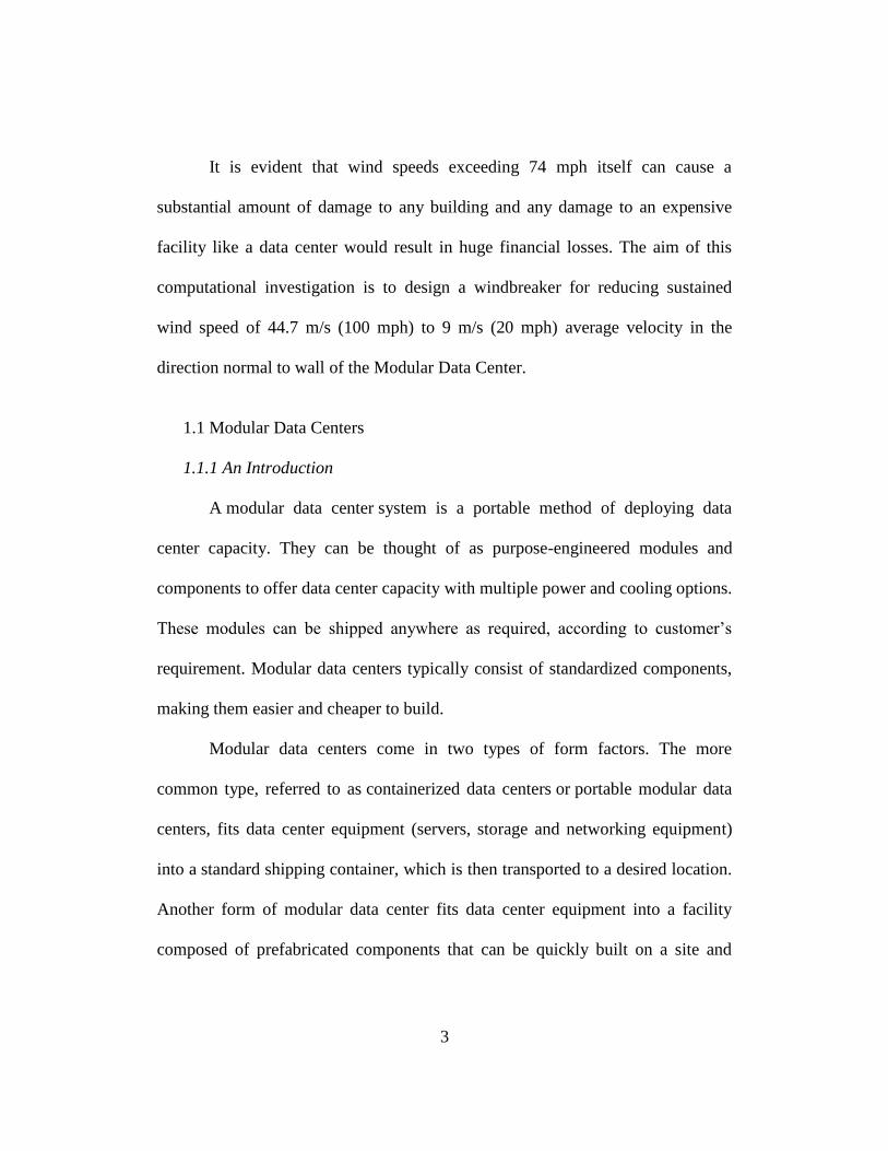
A modular data center system is a portable method of deploying data

center capacity. They can be thought of as purpose-engineered modules and

components to offer data center capacity with multiple power and cooling options.

These modules can be shipped anywhere as required, according to customer’s

requirement. Modular data centers typically consist of standardized components,

making them easier and cheaper to build.

Modular data centers come in two types of form factors. The more

common type, referred to as containerized data centers or portable modular data

centers, fits data center equipment (servers, storage and networking equipment)

into a standard shipping container, which is then transported to a desired location.

Another form of modular data center fits data center equipment into a facility

composed of prefabricated components that can be quickly built on a site and

4

added to as capacity is needed. For example, HP’s version of this type of modular

data center, which it calls Flexible Data Center, is constructed of sheet metal

components that are formed into four data center halls linked by a central

operating building. [3]

Modular data centers provide the option of rapid deployment directly to

the required site, with pre-configured setup, supplied as a fully functional unit.

This leads to savings in time, man power involved in construction and overall

costs in shipping and delivering the equipment. Hence, modular data centers are a

better alternative as compared to the traditional data centers.

Figure 1 Dell EPIC Modular Data Center for eBay [4]

The Dell EPIC MDC has room for 24 racks of IT gear and can have up to

50 kilowatts of power in a rack without melting, for a total of 1.1 megawatts. It

uses outside air cooling and has evaporative cooling (using misting water to chill

5

the air) for when the outside temperature gets too high. Dell has filled up sixteen

of those racks with gear already for eBay as part of the rollout. [4]

1.1.2 Yahoo’s Chicken Coop Data Center

There is an incredible similarity between a traditional chicken coop and

Yahoo’s ‘chicken coop data centers. In this kind of design there are openings in

the floor. The air from below the floor is drawn up through the coop keeping the

chickens cool. The air movement also removes excess moisture. Similar principle

is used in designing the data center, as this concept leads to ventilating a data

center using a full-roof cupola system, which proves to be a great way to cool

computing equipment. The first design was standard fare having a raised-floor

white-space and forced-air cooling.

The company’s second design, Yahoo Thermal Cooling (YTC) uses a

different approach. The white-space in a YTC data center is considered the cool

zone. Hot air exiting the server rack is captured in an enclosed space and forced

up through an inter-cooler. What makes the YTC concept unique is the fact that

server fans move the air. The entire structure acts as an air-handler, wherein the

hot air is allowed to rise via natural convection. Also, the use of evaporative

coolers during the hot summer months along with free cooling, reduces the need

for chiller-systems and air handling equipment. The entry and exhaust of air is

controlled by a louver system which works based upon the internal temperature

6

with the data center. It also consists of fan modules, filter assemblies and

evaporative (water) Inter-Cooling Modules. [5]

The Yahoo Chicken Coop design has three different cooling modes:

Unconditioned Outside Air Cooling: When air temperature is between

70°F and 85°F (21C to 29C), air enters the data-center through louvered

side walls, which is filtered and drawn through the servers by fans housed

in the rack-mounted computing and networking devices. This now-hot

exhaust air after passing through the servers moves up into the attic

through natural convection. The exhaust air continues out of the data

center through the adjustable louvers in the roof-length cupola.

Outside Air Tempered by Evaporative Cooling: When the air temperature

is above 85°F, air takes the same path as the previous case, except that

shortly after entering the outer louvered walls, it is drawn through

saturated media (Inter-Cooling Modules) in order to provide evaporative

cooling to this incoming hot air.

Mixed Outside Air Cooling: When the air temperature is below 70°F,

especially during winter months, heated exhaust air is mixed with

incoming outside air to maintain an air temperature of 70°F. This is

achieved by recirculating fans and a control system which closes the

louvers when the outside air temperature is below 70°F.[5]

7

A similar system is used in other data centers which use the Chicken Coop

design. This design has proved to be very energy-efficient. It was found that,

approximately 36 million gallons of water were saved per year with the chicken

coop design, compared to conventional water-cooled chiller plant designs having

comparable IT loads. Also, this design realized an almost 40 percent cut in the

amount of electricity used relative to industry-typical legacy data centers. [6]

Figure 2 Yahoo Compute Coop Data Center facility[5]

8

Chapter 2

WINDBREAKERS

Windbreaks are barriers used to reduce wind speed and also to redirect the

wind. They usually consist of trees and shrubs, but may also include perennial or

annual crops and grasses, fences, or other materials. As a result of the reduction in

wind speed due to the windbreak, the environmental conditions are modified in

the region behind the windbreak, referred to as sheltered zone.. As wind blows

against a windbreak, there is a high pressure zone created on the windward side

(the side towards the wind) and a low pressure zone created on the leeward side,

and large quantities of air move up and over the top or around the ends of the

windbreak.

As far as the effects of wind on a structure is concerned, for mechanical

damage and loads, the driving force is wind power. Wind power is defined as the

square of wind speed. So, when wind speed is reduced to 25% of original, the

wind power becomes 6.25% of its original value. Wind power is what you feel

when you try and stand up in a strong wind. Clearly, even a small reduction in

wind speed is enough to cause a dramatic reduction in wind power. With erosion

the effect is even more pronounced as dust transport is proportional to wind speed

cubed, or wind speed x wind speed x wind speed.

9

Figure 3 Windbreakers used at airports

A windbreak (also called a wind fence or wind shelter) can reduce wind

speeds by over 50% of the incoming wind speed over large areas, and over 80%

over localized areas. The figure shows reduction in wind speed behind a

windbreak.

Figure 4 Wind speed behind windbreaker as percentage of incoming speed

http://weathersolve.com/wind-shelters/efctvnes-50ft/

10

2.1 Effectiveness of the Windbreak

The effectiveness of a windbreak in reducing the wind speed and altering

the microclimate are determined by various characteristics of the windbreak

structure. These characteristics include: height of the windbreak, distance of the

windbreak from area to be sheltered, density of the windbreak, length and

orientation.

2.1.1 Effect of Height

Windbreak height (H) is an important factor in determining the downwind

area protected by a windbreak. This value varies from windbreak to windbreak. In

farming applications, there are multiple row windbreaks. In this case the height of

the tallest tree-row determines the value of H.

On the windward side of a windbreak, wind speed reductions are

measurable upwind for a distance of 2 to 5 times the height of the windbreak (2H

to 5H). On the leeward side (downwind side), wind speed reductions occur up to

30H downwind of the barrier. Within this protected zone, the structural

characteristics of a windbreak, especially density, determine the extent of wind

speed reductions.[7]

In the case of data centers, it is required that the wind speed is reduced

only in an area immediately after the windbreak, that is just before the point of

entry and exhaust of the air into and out of the data center, respectively. Hence,

11

we do not need protection up to a large distance downwind. So the height H of the

windbreak is chosen equal to the height of the data center itself.

2.1.2 Effect of Distance

Distance of the windbreak from area to be protected also plays an

important role in reducing the wind speeds downwind. It is observed that for a

fixed height, the area protected downwind is fixed. Although, placing the

windbreaker very close to the data center would have the data center in the

protected region, it would also choke the inlet and obstruct the outlet. While

placing the windbreak too far away from the data center would not serve the

purpose, that is reduced wind speed before the inlet and outlet of the data center.

Therefore, it is necessary that the windbreaker is placed at an optimum distance

from the data center in order to achieve its full benefit.

2.1.3 Effect of Density

Windbreak density also referred to as void volume fraction, is the ratio of

the solid portion of the barrier to the total area of the barrier. When the wind is

obstructed by a very dense windbreak, a low pressure develops on the leeward

side. This low pressure area behind the windbreak pulls air coming over the

windbreak downward, creating turbulence and reducing protection downwind. As

void volume fraction of the windbreak increases, the amount of air passing

through the windbreak increases, moderating the low pressure and turbulence, and

increasing the length of the downwind protected area. While this protected area is

12

larger, the wind speed reductions are not as great. By adjusting windbreak density

different wind flow patterns and areas of protection are established.[7]

Figure 5 Effect of density

As windbreaks are mostly used in farming applications, while designing a

windbreak, density should be adjusted to meet landowner objectives. A windbreak

density of 40 to 60 percent provides the greatest downwind area of protection and

provides excellent soil erosion control. To get even distribution of snow across a

field, densities of 25 to 35 percent are most effective, but may not provide

sufficient control of soil erosion. Windbreaks designed to catch and store snow in

13

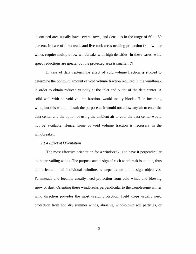
a confined area usually have several rows, and densities in the range of 60 to 80

percent. In case of farmsteads and livestock areas needing protection from winter

winds require multiple row windbreaks with high densities. In these cases, wind

speed reductions are greater but the protected area is smaller.[7]

In case of data centers, the effect of void volume fraction is studied to

determine the optimum amount of void volume fraction required in the windbreak

in order to obtain reduced velocity at the inlet and outlet of the data center. A

solid wall with no void volume fraction, would totally block off an incoming

wind, but this would not suit the purpose as it would not allow any air to enter the

data center and the option of using the ambient air to cool the data center would

not be available. Hence, some of void volume fraction is necessary in the

windbreaker.

2.1.4 Effect of Orientation

The most effective orientation for a windbreak is to have it perpendicular

to the prevailing winds. The purpose and design of each windbreak is unique, thus

the orientation of individual windbreaks depends on the design objectives.

Farmsteads and feedlots usually need protection from cold winds and blowing

snow or dust. Orienting these windbreaks perpendicular to the troublesome winter

wind direction provides the most useful protection. Field crops usually need

protection from hot, dry summer winds, abrasive, wind-blown soil particles, or

14

both. The orientation of these windbreaks should be perpendicular to prevailing

winds during critical growing periods.

Although wind may blow predominantly from one direction for a season,

it rarely blows exclusively from that direction. As a result, protection is not equal

for all areas on the leeward side of a windbreak. As the wind changes direction

and is no longer blowing directly against the windbreak, the protected area

decreases. Again, individual placement depends on the site, the wind direction(s),

and the design objectives.[7]

2.1.5 Effect of Length

Although the height of a windbreak determines the extent of the protected

area downwind, the length of a windbreak determines the amount of total area

receiving protection. For maximum efficiency, the uninterrupted length of a

windbreak should exceed the height; by at least 10:1. This ratio reduces the

influence of end-turbulence on the total protected area. The continuity of a

windbreak also influences its efficiency. Gaps in a windbreak become funnels that

concentrate wind flow, creating areas on the downwind side of the gap in which

wind speeds often exceed open field wind velocities. Where there are gaps, the

effectiveness of the windbreak is diminished. Lanes or field accesses through

windbreaks should be located to minimize this effect or if possible avoided

altogether.[7]

15

Chapter 3

COMPUTATIONAL FLUID DYNAMICS (CFD) ANALYSIS

3.1 Introduction to CFD Analysis

CFD is a branch of Fluid Dynamics which deals with the analysis of

problems involving fluid flow and heat transfer. It uses numerical methods and

algorithms to solve and analyze problems. Computational fluid dynamics is

applied to simulate and analyze the behavior of fluids in various systems. The

major advantage of numerical methods is that, the problem is discretized based on

certain parameters and solved. A mathematical model is generated, which

represents to actual physical system and then it can be solved and analyzed. In

this case the study involves the effect of fluid (air) flow past the Modular Data

Center and the Windbreaker and how this affects the velocity, pressure and other

characteristics in the system.

CFD is concerned with the numerical simulation of fluid flow, heat

transfer and related processes such as radiation. The objective of CFD is to

provide the engineer with a computer-based predictive tool that enables the

analysis of the air-flow processes occurring within and around different

equipment, with the aim of improving and optimizing the design of new or

existing equipment.[8]

16

3.2 Governing Equations

The numerical solution for most problems are obtained by solving a series

of three differential equations, collectively referred to as the Navier-Stokes’

Equations. These differential equations are the conservation of mass, conservation

of momentum and conservation of energy.

But in this particular case, temperature is constant and the effect of flow is

analyzed. Hence, only conservation of mass and conservation of momentum

equations are solved.

In general form,

The conservation of mass is given by:

𝜕(⍴)

𝜕𝑡+∇. (⍴u)=0

The conservation of momentum is given by:

𝜕(⍴𝑢)

𝜕𝑡+ (⍴𝑢. 𝛻)𝑢 = 𝛻. (µ𝛻𝑢) − 𝛻𝑝 + ⍴𝑓

The solution domain is the region or space within which these differential

equations are solved. The solutions are obtained by imposing certain boundary

conditions for this solution domain. The boundary conditions for most problems

include ambient temperature, pressure, wind conditions and other environmental

conditions. Also, if there is heat transfer involved then, type of heat transfer, such

as conduction, convection or even radiation are considered. The conditions at the

domain wall are also specified, whether they are open, closed or symmetrical in

17

nature. The fluid properties like density, viscosity, diffusivity and specific heat

need to be specified. [9]

The governing equations for many problems are solved using numerical

techniques like Finite Element Method, Finite Volume Method and Finite

Difference Method. In FEM, the elements are varied and approximated by a

function, in FVM the equations are integrated around a mesh element whose

volumes are considered and in FDM the differential terms are discretized for each

element.

In the CFD technique used in FloTHERM 10.1, the conservation equations

are discretized by sub-division of the domain of integration into a set of non-

overlapping, continuous finite volumes referred to as ‘grid cells’, ‘control cells’ or

quite simply as ‘cells’. The governing equations are solved by considering the

volume of the grid cells and the variables to be calculated are situated at the

center of these grid cells.

The finite volume method is more advantageous than other computational

methods as it the governing equations are conserved even on coarse grids and it

also does not limit cell shape. A set of algebraic equations are used for

discretizing the results, each of which relates the value of a variable in a cell to its

value in the nearest-neighbor cells.

For example let T denote the temperature, this can be calculated using the

algebraic equation:

18

T= 𝐶0𝑇0+𝐶1T1+𝐶2𝑇2+⋯𝐶𝑛𝑇𝑛+𝑆

𝐶0+𝐶1+𝐶2+⋯𝐶𝑛

Where T0 represents temperature value in the initial cell, T1, T2….,Tn are

values in the neighboring cells; C0, C1, C2,…, Cn are the coefficients that link

the in-cell value to each of its neighbor-cell values. S denotes the terms that

represent the influences of the boundary conditions.

These algebraic equations are solved for the variables like T, u, v, w and p.

This means that if there are ‘n’ cells in the solution domain, a total of ‘5n’

equations are solved.

Figure 6 Representation of a 3D grid

19

3.3 Turbulence Modeling

A flow is said to be turbulent when the fluid undergoes irregular

fluctuations or mixing. The velocity of the fluid at a point is continuously

undergoing changes in both magnitude and direction, as opposed to laminar flow

wherein the fluid moves in smooth paths or layers. Usually fluid with large

Reynolds number are considered to be turbulent, while fluids with low Reynolds

number are considered laminar. FloTHERM 10.1 uses two common methods to

model turbulent flows: LVEL turbulence model and K-Epsilon turbulence model.

3.3.1 LVEL Turbulence Model

The LVEL turbulence model requires only few terms to determine the

effective viscosity. They are nearest wall distance (L), the local velocity (VEL)

and the laminar viscosity. In this model, Poisson’s equation is solved initially to

calculate the maximum length scale and local distance to nearest wall.

D = (|∇∅|2 +2∅)1/2

L= D-|∇∅|

Where |∇∅| = -1 and ∅ = 0 (which is boundary condition at the wall)

∅ is the dependent variable. [10]

3.3.2 K-Epsilon Turbulence Model

The K-Epsilon turbulence model solves the governing equations along

with another two additional equations, namely, the kinetic energy of turbulence

(k) and the dissipation rate of kinetic energy turbulence (ε). It is also known as the

20

two equation model and is used widely in turbulent flow modeling.[10] The two

additional transport equations solved are:

Kinetic Energy of turbulence equation (k)

Dissipation rate of kinetic energy of turbulence (ε)

3.4 Meshing and Grid Constants

Grid constraints allow you to attach minimum grid requirements to a

geometry so as to make sure that there is sufficient grid coverage wherever it is

located in the solution domain. Grid constraints are used to specify minimum and

maximum number of cells across a geometry.

Meshing is an important feature of any CFD software, since if the model

created is not properly meshed, the results of the simulation would be inaccurate.

The mesh needs to be fine in critical areas and can be coarse in areas of less

importance. Keeping the mesh fine in critical areas would give the most accurate

results. Also, a mesh sensitivity analysis can determine when the solution has

reached grid independence. Grid independence is the point at which, addition of a

ijijt

k

t EEkgraddivkdivt

k.2)(

)(U

kCEE

kCgraddivdiv

tijijt

t

2

21.2)(

)(

U

21

large number grid cells has no further effect on the solution. FloTHERM 10.1

uses a Cartesian grid system and the values of any variable are calculated at the

center of each grid cell. While meshing the model created in FloTHERM 10.1

there is an option of keeping the grid fine, medium or coarse. Also, localizing a

grid is another option to improve the mesh. In this feature, the grid lines from two

different regions do not interfere. The point where gridlines meet the edges of an

object, they get truncated.

3.5 Smart Parts in FloTHERM 10.1

3.5.1 Cuboid

This is the most basic smart part in FloTHERM 10.1. It is used in

representing most objects in the system. It is a solid block and can be used to

represent any solid object like the external structure of the modular data center, a

solid wall, etc. It also has the option to be collapsed to represent a plate.

3.5.2 Resistance

The resistance smart part is used to define region which acts as a barrier or

a resistance to a flow. They can be collapsed, angled or non-collapsed depending

on the requirement. They usually represent a porous media. The void volume

fraction can be defined from the resistance library depending on the requirement.

In this model the resistance smart part is used to represent a porous windbreaker.

Different values of void volume fraction are given to the resistance to simulate a

22

windbreaker with varying void volume fraction. In other applications, this smart

part is used for modelling filters and vents.

3.5.3 Enclosure

The enclosure smart part is a hollow part which can used to define the

outer boundaries of an object or system. It is cuboidal in shape and each side of

the cuboid can have independent properties. We can remove certain sides of the

enclosure and keep the remaining. In this manner we can use the enclosure smart

part to simulate a wind tunnel, by keeping two the sides along its length, open.

The thickness of the enclosure smart part can be specified or it can be kept as thin.

It is also used to model racks, servers, etc.

3.5.4 Source

The source smart part is used to represent objects that require power to be

defined. This smart part is used to simulate a wind source, with a fixed velocity

assigned to it. The direction of the wind source can be defined as needed. The

source area is made equal to the area of the open side of the enclosure, such that

all the wind source velocity is channeled through the enclosure, thus acting as a

wind tunnel.

3.5.5 Monitor Points

Monitor points are used to determine various parameters at critical points

within the solution domain. They are usually used to monitor temperature or

pressure at certain critical points within the system. In this case, monitor points

23

are used to monitor pressure in regions close to the inlet and exhaust of the

modular data center.

3.5.6 Region

This smart part is used for two main purposes. The first one being to

create a refined mesh in a particular area of interest. A region can be created in a

particular area where a finer mesh is required and the mesh density can be

improved in that particular region using the Localize feature. Another use of the

region is that it can be used in post processing. The values of different parameters

like, velocity, pressure, speed, temperature can be determined within a particular

region.

3.5.7 Command Center

The command center in FloTHERM 10.1 can be used to generate and

solve different scenarios at the same time, enabling you to quickly see the effects

of changing certain selected variables. This enables us to vary multiple parameters

and see their individual or combined effect on the total system. Parametric and

mesh sensitivity analysis can be performed using the command center. Mesh

sensitivity analysis can be performed by varying the number of grid cells and

studying its effect on the other parameters, by performing all the trials

simultaneously. A parametric analysis can be performed for different components,

for example, a parametric analysis of the fence is performed by varying

parameters like distance from the MDC, void volume fraction and height.

24

Basically, the procedure that is followed while using the command center

is that, a datum case is loaded as the project. Then in the command center, the

parameters that are to be varied, called as the Input Variables are selected. This

generates the different scenarios based on the number cases created. There is a

graphical input tab which enables us to view what change has occurred in the

model, due to the scenarios created by the input variables defined. The results that

are required, for example, pressure, temperature, velocity, speed, etc. can be

selected in the Output Variables tab. These can be viewed in the Scenario Table

generated along with the input variables as well. There is also a tab called

Solution Monitoring, for monitoring the solution and check for convergence.

25

Chapter 4

DESCRIPTION OF THE MODEL

The Computational Fluid Dynamics model is of a chicken coop modular

data center and the two windbreakers, which are located at a certain distance in

front of the inlet and exhaust of the MDC. Only the external structure of the MDC

is modelled as this study is concerned with the wind loading on the external

structure itself. The model was entirely created using FloTHERM 10.1 smart

parts.

4.1 Description of the Modular Data Center

The modular data center modelled is a chicken coop modular data center,

whose structure is similar to the Yahoo’s Chicken Coop Data Center. It has two

sections, the lower section which is the IT pod, which consists of all the IT

equipment, filtration units, fans, etc. It also consists of the inlets for the ambient

air to enter the data center, which is used for cooling purposes. The top section

consists of the chicken coop or chimney, which acts as the exhaust for the hot air

that rises from the hot aisle within the modular data center.

26

Figure 7 3D model of MDC

4.2 Description of the Windbreaker

The windbreaker used in this model is of a split wall type. One wall is

placed on the ground and the second one is placed on top of the IT pod, in front of

the chicken coop (exhaust). The height of the windbreaker is chosen equal to the

height of the MDC. The windbreakers are modelled using the resistance smart

part in FloTHERM 10.1. This allows the windbreaker to be modelled as a porous

body with varying resistances. The initial case chosen was with 5% void volume

fraction.

27

Figure 8 Split Wall configuration schematic

4.3 Description of the CFD Model

4.3.1 Dimensions of the Model

Table 2 Dimensions of the model

Length Width Height

Lower portion of MDC 14160 5450 3740

Upper portion of MDC 2200 5450 2000

Lower portion of windbreaker 100 5450 3740

Upper portion of windbreaker 100 5450 2000

4.3.2 Model Setup

The model setup used for all the cases was as follows:

Type of Solution was set to Flow Only

Dimensionality was selected as 3-Dimensional

28

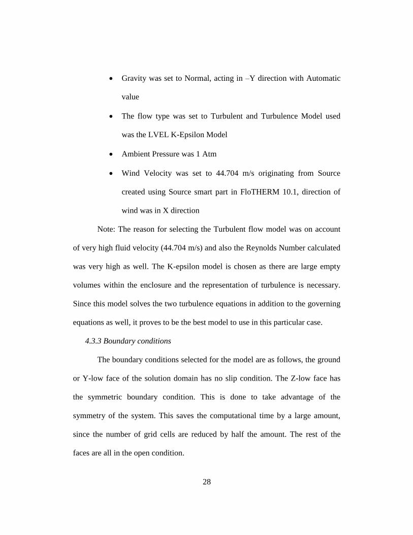
Gravity was set to Normal, acting in –Y direction with Automatic

value

The flow type was set to Turbulent and Turbulence Model used

was the LVEL K-Epsilon Model

Ambient Pressure was 1 Atm

Wind Velocity was set to 44.704 m/s originating from Source

created using Source smart part in FloTHERM 10.1, direction of

wind was in X direction

Note: The reason for selecting the Turbulent flow model was on account

of very high fluid velocity (44.704 m/s) and also the Reynolds Number calculated

was very high as well. The K-epsilon model is chosen as there are large empty

volumes within the enclosure and the representation of turbulence is necessary.

Since this model solves the two turbulence equations in addition to the governing

equations as well, it proves to be the best model to use in this particular case.

4.3.3 Boundary conditions

The boundary conditions selected for the model are as follows, the ground

or Y-low face of the solution domain has no slip condition. The Z-low face has

the symmetric boundary condition. This is done to take advantage of the

symmetry of the system. This saves the computational time by a large amount,

since the number of grid cells are reduced by half the amount. The rest of the

faces are all in the open condition.

29

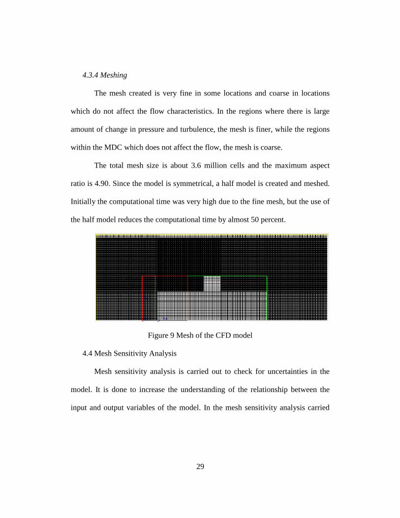
4.3.4 Meshing

The mesh created is very fine in some locations and coarse in locations

which do not affect the flow characteristics. In the regions where there is large

amount of change in pressure and turbulence, the mesh is finer, while the regions

within the MDC which does not affect the flow, the mesh is coarse.

The total mesh size is about 3.6 million cells and the maximum aspect

ratio is 4.90. Since the model is symmetrical, a half model is created and meshed.

Initially the computational time was very high due to the fine mesh, but the use of

the half model reduces the computational time by almost 50 percent.

Figure 9 Mesh of the CFD model

4.4 Mesh Sensitivity Analysis

Mesh sensitivity analysis is carried out to check for uncertainties in the

model. It is done to increase the understanding of the relationship between the

input and output variables of the model. In the mesh sensitivity analysis carried

30

out in this case, the input variable is the number grid cells is varied and its effect

on the output variables like speed and pressure are studied.

The following mesh sensitivity analysis was carried out on the model.

Table 3 Mesh Sensitivity analysis

Grid independence was achieved at 3.6 million cells with maximum aspect

ratio of 4.9.

Figure 10 Mesh Sensitivity Analysis

77.27.47.67.8

88.28.48.68.8

99.2

0 5000000 10000000

Spee

d L

ow

Reg

ion (

m/s

)

Number of grid cells

Mesh Sensitivity

Mesh Sensitivity

Cumulative total Speed % skewness

852681 9.03384 0

1878199 7.80365 13.62

2737552 7.91442 1.41

3604554 7.94467 0.37

4854640 7.95409 0.13

6580910 7.94887 0.06

31

Figure 11 Half-model with boundary conditions

4.5 Scenarios Considered

The two main parameters that were considered in this investigation were

Distance of the windbreakers from the MDC and void volume fraction of the

Windbreakers. The initial case considered was wherein, both the upper and lower

wall were taken at 2 m from the MDC. The distance was then varied in the steps

of 0.5 m. A total of six cases were considered, at distances of 0.5,1, 1.5, 2.5, 3 and

3.5 meters. Void volume fraction was varied from 5%, 10%, 20% and 30%. Void

volume fraction greater than 30% would not be serve the purpose as the wind

speeds at the walls of the MDC would be higher than 20 mph, irrespective of the

position of the windbreaker, which is not desirable.

Symmetry BC

Half model of MDC

No-slip BC

Half model of Windbreaker

32

Chapter 5

RESULTS AND CONCLUSION

The following results were obtained by varying the distance of the

windbreaker from the MDC and the void volume fraction of the windbreaker. The

results were monitored at a region which is 1 ft. (0.3 m) away from the MDC.

Assumption: The maximum wind speed that is acceptable at a distance of

1 ft. from the MDC is 20 mph (9 m/s).

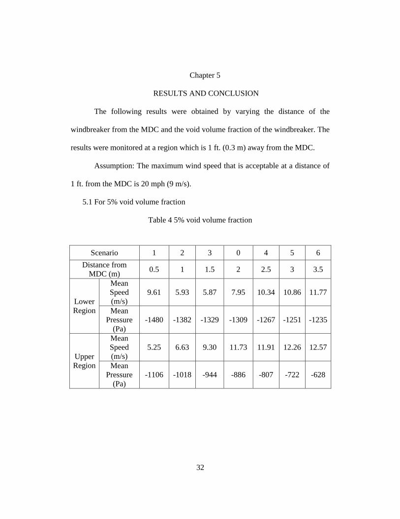
5.1 For 5% void volume fraction

Table 4 5% void volume fraction

Scenario 1 2 3 0 4 5 6

Distance from

MDC (m) 0.5 1 1.5 2 2.5 3 3.5

Lower

Region

Mean

Speed

(m/s)

9.61 5.93 5.87 7.95 10.34 10.86 11.77

Mean

Pressure

(Pa)

-1480 -1382 -1329 -1309 -1267 -1251 -1235

Upper

Region

Mean

Speed

(m/s)

5.25 6.63 9.30 11.73 11.91 12.26 12.57

Mean

Pressure

(Pa)

-1106 -1018 -944 -886 -807 -722 -628

33

For the lower region, maximum reduction in speed is observed when the

windbreaker is placed at 1.5 m from MDC and for upper region, it is 0.5 m from

MDC.

5.1.1 Velocity profile at 0.5m from MDC

Figure 12 Lower wall at 0.5m from MDC

34

Figure 13 Upper wall at 0.5m from MDC

5.1.2 Velocity profile at 2m from MDC

Figure 14 Lower wall at 2m from MDC

35

Figure 15 Upper wall at 2m from MDC

5.1.3 Velocity profile at 3.5m from MDC

Figure 16 Lower wall at 3.5m from MDC

36

Figure 17 Upper wall at 3.5m from MDC

Figure 18 Particle track for 5% void volume fraction of windbreaker

37



For the lower region, best results are observed when the windbreaker is

placed at 1.5 m from MDC and for upper region, it is 1 m from MDC.

Scenario 1 2 3 0 4 5 6

Distance from

MDC (m) 0.5 1 1.5 2 2.5 3 3.5

Lower

Region

Mean

Speed

(m/s)

11.90 7.10 5.62 6.32 10.18 11.82 11.49

Mean

Pressure

(Pa)

-1165 -1150 -1144 -1130 -1156 -1168 -1199

Upper

Region

Mean

Speed

(m/s)

5.98 5.39 6.73 9.54 10.13 11.70 11.86

Mean

Pressure

(Pa)

-845 -866 -866 -831 -799 -788 -806

38

5.3 For 20% void volume fraction.


It is observed that for the lower region least wind speed is attained when

the windbreaker is placed at 3 m from MDC and for the upper region least wind

speed is attained at 2 m from MDC.

Scenario 1 2 3 0 4 5 6

Distance from

MDC (m) 0.5 1 1.5 2 2.5 3 3.5

Lower

Region

Mean

Speed

(m/s)

21.27 10.58 7.61 5.69 4.68 5.05 7.05

Mean

Pressure

(Pa)

-431 -690 -746 -775 -797 -807 -842

Upper

Region

Mean

Speed

(m/s)

8.11 7.38 5.28 4.57 6.61 8.68 10.3

Mean

Pressure

(Pa)

-523 -591 -598 -592 -579 -556 -524

39

Figure 19 Particle track for 20% void volume fraction of windbreaker



It is observed that for lower region, least wind speed is attained at 3.5 m

from the MDC and for the upper region, least wind speed is at 3 m from MDC.

Scenario 1 2 3 0 4 5 6

Distance from MDC

(m) 0.5 1 1.5 2 2.5 3 3.5

Lower

Region

Mean Speed

(m/s) 27.2 18.15 11.80 8.52 7.61 6.26 5.07

Mean

Pressure

(Pa)

336 -132 -312 -361 -397 -424 -461

Upper

Region

Mean Speed

(m/s) 6.74 9.50 9.10 7.57 5.86 4.72 4.89

Mean

Pressure

(Pa)

160 -375 -408 -422 -422 -416 -418

40

5.5 For 40% void volume fraction.


It is observed that for lower region, least wind speed is attained at 3.5 m

from the MDC and for the upper region, least wind speed is at 3 m from MDC.

5.6 Plot of Normalized Speed vs Windbreaker distance

The speeds determined at both upper and lower regions of the MDC were

normalized by dividing it by a factor, 9 (maximum acceptable speed). All the

points lying within the shaded region are acceptable configurations.

Scenario 1 2 3 0 4 5 6

Distance from

MDC (m) 0.5 1 1.5 2 2.5 3 3.5

Lower

Region

Mean

Speed

(m/s)

26.46 23.62 18.21 14.38 11.58 11.14 7.83

Mean

Pressure

(Pa)

454 410 368 91 -71 -68 -38

Upper

Region

Mean

Speed

(m/s)

14.98 8.33 12.23 12.18 12.36 11.96 10.44

Mean

Pressure

(Pa)

-322 -267 -304 -299 -310 -316 -322

41

Figure 20 Graph of normalized speed vs windbreaker distance from MDC

From the above plot the acceptable configurations for the windbreaker

where wind speed is less than 9m/s, were

5% at 1m

10% at 1m and 1.5m

20% at 1.5m, 2m, 2.5m and 3m

30% at 2m, 2.5m, 3m and 3.5m

5.6 Conclusion

The following conclusions can be drawn from this analysis:

0

0.25

0.5

0.75

1

1.25

1.5

1.75

2

2.25

2.5

2.75

3

3.25

0 1 2 3 4

Nio

rmal

ized

spee

d

Windbreaker distance from MDC (m)

Speed vs Windbreaker distance

5% Lower

5% Upper

10% Lower

10% Upper

20% Lower

20% Upper

30% Lower

30% Upper

40% Lower

40% Upper

42

The steady state analysis was conducted and the flow of the air across the

MDC can be analyzed for various parameters like speed, pressure, turbulence.

There was a substantial reduction in wind speed due to the presence of the

windbreakers.

Wind speed reduction below the desired value was obtained at various

distances and void volume fractions for both the upper and lower regions.

Optimum configuration would be when the windbreaker with 30% void

volume fraction was placed at a distance of 3.5 m from the MDC. This would

be the optimum choice over the other options because building a windbreaker

with 30% void volume fraction would be cheaper and less material would be

required. Also having it at 3.5m away from the MDC would improve

workability and provide ease of access around the MDC.

43

Chapter 6

SCOPE AND FUTURE WORK

Transient analysis to conduct in-depth analysis of the low field. This would

help to gain a better understanding of the flow around the MDC.

Structural design of the windbreaker and also choice of material.

3D stress analysis of the windbreaker.

Varying other parameters of the windbreaker such as height and orientation

and study the combined effects of varying all parameters.

44

References

[1] [Online] Available: http://www.spc.noaa.gov/faq/tornado/beaufort.html

[2] [Online] Available: http://www.nhc.noaa.gov/aboutsshws.php

[3] “Modular Data Center”, Wikipedia, [Online]. Available:

http://en.wikipedia.org/wiki/Modular_data_center

[4] [Online] Available: http://www.enterprisetech.com/2013/09/27/ebay-juices-

utah-modular-data-center-fuel-cells-waste-heat/

[5] Yahoo! Compute Coop (YCC): A Next-Generation Passive Cooling Design

for Data Centers, AD Robison, Chris Page, Bob Lytle

[6] [Online] Available: http://www.datacenterdynamics.com/design-

strategy/yahoos-compute-coop-is-not-for-chickens/93474.fullarticle

[7] [Online] Available: http://extension.psu.edu/plants/plasticulture/production-

details/windbreaks

[8] [Online] Available: http://www.bdi.aero/

45

Biographical Information

Prasad Pramod Revankar was born in Goa, India. He received his

Bachelor’s degree in Mechanical Engineering from Goa University, India in 2012.

He completed his Master of Science degree in Mechanical Engineering at the

University of Texas at Arlington in May 2015.

His primary research areas include Computational Fluid Dynamics. He has

worked on the CFD analysis of the flow past a Modular Data Centers. The project

he has worked on was designing a windbreaker to reduce high speed wind loading

on modular data centers.

He joined the EMNSPC research team under Dr. Dereje Agonafer in

November, 2014.

USE OF A WINDBREAKER TO MITIGATE HIGH SPEED WIND …

Documents

Transcript of USE OF A WINDBREAKER TO MITIGATE HIGH SPEED WIND …