
Upgrade of SBAS Simulator User Manual - · PDF fileLANOPWE Longitude of Ascending Node of...
86
Iguassu Software Systems Ref : SBAS-SIM-MANUAL Issue : 1 Rev. : 3 Date : 02/11/2015 Page : 1 Name & Function Signature Date Prepared by: Jiri Doubek, Igor Kokorev 04/05/2015 Checked by: Authorised by: Approved by: Jiri Doubek, Project Manager 02/11/2015 Upgrade of SBAS Simulator User Manual
Transcript of Upgrade of SBAS Simulator User Manual - · PDF fileLANOPWE Longitude of Ascending Node of...

Iguassu Software Systems
Ref : SBAS-SIM-MANUAL
Issue : 1 Rev. : 3 Date : 02/11/2015 Page : 1
Name & Function Signature Date
Prepared by: Jiri Doubek, Igor Kokorev 04/05/2015
Checked by:
Authorised by:
Approved by: Jiri Doubek, Project Manager 02/11/2015
Upgrade of SBAS Simulator
User Manual

Iguassu Software Systems
Ref : SBAS-SIM-MANUAL
Issue : 1 Rev. : 3 Date : 02/11/2015 Page : 2
DOCUMENT INFORMATION
Contract data
Contract Number 4000111120/14/NL/CBi
Contract Issuer ESA - ESTEC
Distribution List
Iguassu Software
Systems
Jiri Doubek
Miroslav Houdek
Daniel Chung
Igor Kokorev
ESA
Jaron Samson
Constantin Alexandru Pandele
Katarzyna Urbanska
Christelle Iliopoulos
Document Change Record
Iss./Rev. Date Section/Page Change Description
1.0 04/05/2015 all Document proposal
1.1 02/07/2015 2.3.2.1 Command line simulations
1.2 19/08/2015
4.1.2.1,
4.5.4.1,
4.5.4.2, 5.10
GEO satellites longitude, ionospheric
settings, DOC simulations
1.3 02/11/2015
3.5, 5.3.4, 5.6,
5.8.2, 5.8.3,
5.11.2, 6.1.1
Region graphs: changes in colour scale
and in area layers.

Iguassu Software Systems
Ref : SBAS-SIM-MANUAL
Issue : 1 Rev. : 3 Date : 02/11/2015 Page : 3
1 Introduction The present document is the User Manual applicable to “Upgrade of SBAS Simulator” project.
The objective of this activity was to update the SBAS Simulator, a tool developed under the
ESA PECS programme in 2009, which provides an environment where users can perform
various simulations of Satellite Based Augmentation Systems (SBAS). The upgrade of the
SBAS Simulator supports both, the analysis of the performance of the current EGNOS system,
as well as the future evolution of EGNOS.
1.1 Document Structure
This document is organised as follows:
Section 1 provides an introduction, the table of contents and a list of documents and acronyms
Section 2 describes the operations environment
Section 3 gives a short start-up guide
Section 4 details all SBAS Simulator settings
Section 5 describes all analyses and tools
Section 6 provides information to region graphs
Section 7 gives an overview of SBAS Simulator files
1.2 Document Status
This is a definitive issue of this document.

Iguassu Software Systems
Ref : SBAS-SIM-MANUAL
Issue : 1 Rev. : 3 Date : 02/11/2015 Page : 4
1.3 Table of Contents
1 Introduction ........................................................................................................................ 3
1.1 Document Structure .................................................................................................... 3
1.2 Document Status ......................................................................................................... 3
1.3 Table of Contents ......................................................................................................... 4
1.4 Applicable Documents ................................................................................................. 7
1.5 Reference Documents ................................................................................................. 7
1.6 Terms, definitions and abbreviated terms .................................................................. 7
1.7 Purpose of the Software ............................................................................................ 10
1.8 External view of the software .................................................................................... 10
2 Operations environment .................................................................................................. 10
2.1 General ...................................................................................................................... 10
2.2 Hardware configuration ............................................................................................ 12
2.3 Software configuration .............................................................................................. 12
2.3.1 Applet configuration .......................................................................................... 12
2.3.2 Standalone application configuration ................................................................ 12
2.4 Operation constraints ................................................................................................ 14
3 Getting Started ................................................................................................................. 14
3.1 Introduction ............................................................................................................... 14
3.2 Sample DOP analysis .................................................................................................. 15
3.2.1 Running the simulator ........................................................................................ 15
3.3 Constellations and satellites ...................................................................................... 16
3.4 Simulation time and area .......................................................................................... 16
3.5 DOP options and analysis .......................................................................................... 16
4 Settings ............................................................................................................................. 17
4.1 Space segment settings ............................................................................................. 18
4.1.1 Satellite settings ................................................................................................. 18
4.1.2 Adding and removing satellite from a constellation .......................................... 26
4.1.3 Adding and removing a constellation ................................................................ 27
4.1.4 Setting the constellation to the default state .................................................... 30

Iguassu Software Systems
Ref : SBAS-SIM-MANUAL
Issue : 1 Rev. : 3 Date : 02/11/2015 Page : 5
4.1.5 Constellation source ........................................................................................... 31
4.1.6 Constellation settings ......................................................................................... 35
4.1.7 Frequency mode and frequency values ............................................................. 37
4.2 User segment settings ............................................................................................... 38
4.2.1 Geographical area settings ................................................................................. 38
4.2.2 User mask settings ............................................................................................. 39
4.2.3 Service settings ................................................................................................... 39
4.3 Ground segment settings .......................................................................................... 39
4.3.1 RIMS selection .................................................................................................... 40
4.3.2 RIMS configuration ............................................................................................. 41
4.3.3 RIMS network configuration .............................................................................. 44
4.3.4 RIMS error distribution ...................................................................................... 44
4.4 Time settings .............................................................................................................. 45
4.5 Macro-model settings ................................................................................................ 46
4.5.1 Constellation sigma values ................................................................................. 47
4.5.2 UDRE model ........................................................................................................ 49
4.5.3 DFRE model ........................................................................................................ 50
4.5.4 Ionospheric model .............................................................................................. 51
4.5.5 SBAS settings ...................................................................................................... 55
4.5.6 XPL dynamic conditions ...................................................................................... 56
4.5.7 Navigation solution unknowns ........................................................................... 58
4.6 Working directory and scenario folder...................................................................... 59
4.7 Scenario ..................................................................................................................... 59
5 Analyses and Tools ........................................................................................................... 60
5.1 General computations ............................................................................................... 61
5.2 Computations of satellite variance (σ) ...................................................................... 62
5.3 DOP ............................................................................................................................ 63
5.3.1 Availability for a point ........................................................................................ 63
5.3.2 Statistics for a point ............................................................................................ 64
5.3.3 Availability for a region ...................................................................................... 65

Iguassu Software Systems
Ref : SBAS-SIM-MANUAL
Issue : 1 Rev. : 3 Date : 02/11/2015 Page : 6
5.3.4 Statistics for a region .......................................................................................... 65
5.4 NSE ............................................................................................................................. 65
5.5 XPL ............................................................................................................................. 66
5.6 Availability ................................................................................................................. 67
5.7 Continuity .................................................................................................................. 69
5.8 IONO .......................................................................................................................... 70
5.8.1 IPP location ......................................................................................................... 71
5.8.2 IGP statistics ....................................................................................................... 71
5.8.3 Sigma GIVE calculation ....................................................................................... 72
5.9 Monitoring ................................................................................................................. 73
5.10 DOC simulations ........................................................................................................ 74
5.10.1 XDOC ................................................................................................................... 75
5.10.2 IDOC .................................................................................................................... 76
5.10.3 ADOC .................................................................................................................. 76
5.11 Coverage, elevation, ground tracks ........................................................................... 77
5.11.1 Coverage ............................................................................................................. 77
5.11.2 Elevation ............................................................................................................. 78
5.11.3 Ground tracks ..................................................................................................... 79
5.12 Delta map .................................................................................................................. 80
5.13 3D view ...................................................................................................................... 81
5.14 Sky plot ...................................................................................................................... 82
6 Graphs .............................................................................................................................. 82
6.1 Region graph .............................................................................................................. 83
6.1.1 Region graph controls ........................................................................................ 83
7 SBAS Simulator Files ......................................................................................................... 84
7.1 Simulation steps ........................................................................................................ 84
7.2 Data and meta-files ................................................................................................... 84

Iguassu Software Systems
Ref : SBAS-SIM-MANUAL
Issue : 1 Rev. : 3 Date : 02/11/2015 Page : 7
1.4 Applicable Documents
Reference Title
[AD1] Statement of Work, Ref. ESA-DTEN-NF-SoW/03982, Issue 1, Revision 0, 26/03/2013
1.5 Reference Documents
Reference Title
[RD1] SBAS Simulator User Manual, www.iguassu.cz/sbas-sim/sbas_sim_manual.pdf
[RD2] SBAS Simulator Upgrade, TN 1- RIMS error over bound; Ref.: SBAS-SIM-TN-01-0.3; Issue: 0; Revision: 3; Date: August 18, 2014
[RD3] Minimum Operational Performance Standards (MOPS) for airborne navigation equipment (2D and 3D) using the Global Positioning System (GPS) augmented by the Wide Area Augmentation System (WAAS)
[RD4] Ionospheric Macro Model for SBAS Service Volume Simulations; S. Schlueter; Issue: 1, Revision: 1; Date: February 9, 2015
[RD5] IS-GPS-200F; Revision: F; September 21, 2011
[RD6] Computation method for SBAS continuity; F. Salabert; NSP March 2013 WGW/flimsy8
1.6 Terms, definitions and abbreviated terms
Acronym Details
AD Applicable Documents
ADOC Advanced Depth Of Coverage
agl Almanac GLONASS
APV Approach Procedure with Vertical Guidance
CSV Comma Separated Values
CRC Cyclic Redundancy Check
df Dual Frequency
DFRE Dual Frequency Range Error
DOC Depth Of Coverage

Iguassu Software Systems
Ref : SBAS-SIM-MANUAL
Issue : 1 Rev. : 3 Date : 02/11/2015 Page : 8
Acronym Details
DOP Dilution Of Precision
ECAC European Civil Aviation Conference
ECEF Earth-Centered, Earth-Fixed
EGNOS European Geostationary Navigation Overlay Service
EMS EGNOS Message Server
ENP European Neighbourhood Policy
ENU East North Up
ESA European Space Agency
EPO EGNOS Project Office
flt Fast and Long Term correction
GDOP Geometric Dilution Of Precision
GEO Geostationary (satellite/constellation)
GIVE Grid Ionospheric Vertical Error
GPS Global Positioning System
HAL Horizontal Alert Limit
HDOP Horizontal Dilution Of Precision
HNSE Horizontal Navigation System Error
HPL Horizontal Protection Level
IDOC Inverse Depth Of Coverage
IGP Ionospheric Grid Point
IONEX IONosphere map EXchange format
IOV In-Orbit Validation
ISS Iguassu Software Systems
IPP Ionospheric Pierce Point
JRE Java Runtime Environment
LANOPWE Longitude of Ascending Node of Orbit Plane at Weekly Epoch
LPV Localiser Performance with Vertical Guidance
LTC Long-Term Corrections
MEO Medium Earth Orbit (satellite)
MOPS Minimum Operational Performance Standards
MT Message Type

Iguassu Software Systems
Ref : SBAS-SIM-MANUAL
Issue : 1 Rev. : 3 Date : 02/11/2015 Page : 9
Acronym Details
NPA Non-Precision Approach
NSE Navigation System Error
OS Operating System
PA Precision Approach
PC Personal Computer
PDOP Positional Dilution Of Precision
QZSS Quasi-Zenith Satellite System
RAAN Right Ascension of the Ascending Node
RD Reference Document
RIMS Ranging and Integrity Monitoring Station(s)
RINEX Receiver Independent Exchange Format
SBAS Satellite Based Augmentation System
sf Single Frequency
SOW Seconds of Week
TDOP Time Dilution Of Precision
TLE Two Line Elements
TN Technical Note
toa Time of Applicability
UDRE User Differential Range Error
UIRE User Ionospheric Range Error
UIVE User Ionospheric Vertical Error
UTC Universal Coordinated Time
VAL Vertical Alert Limit
VDOP Vertical Dilution Of Precision
VNSE Vertical Navigation System Error
VPL Vertical Protection Level
XAL Alert Limits
XDOC Depth Of Coverage
XPL Protection Levels

Iguassu Software Systems
Ref : SBAS-SIM-MANUAL
Issue : 1 Rev. : 3 Date : 02/11/2015 Page : 10
1.7 Purpose of the Software
The principle use of the Upgrade of SBAS Simulator is to simulate the environment of SBAS
systems. The user can configure in detail the space, ground and user segment. The software
is capable to perform simulation in single and dual frequency mode and visualise results in
exportable graphs. The main benefit is to show the future potentials of SBAS systems and
multi constellation solutions.
1.8 External view of the software
The software can run without any external files. Anyway it supports loading configuration
files that store all possible settings of the tool. No restrictions apply to configuration files.
2 Operations environment
2.1 General
SBAS Simulator is written in Java and requires the JRE to be installed. It is a multi-platform
application and can be run in any OS supporting Java. The tool can be started as a
standalone application or as an applet from the web browser. Applet version requires
configuration of the Java security. The site running the applet shall be included in the Java
Exception Site List (Figure 1). User can also switch the Java Security Level to medium, but it is
not recommendable. Running the tool in the browser also requires accepting the Java
Security Warning (Figure 2).

Iguassu Software Systems
Ref : SBAS-SIM-MANUAL
Issue : 1 Rev. : 3 Date : 02/11/2015 Page : 11
Figure 1: Java Exception Site List. In this example the software runs under the www.iguassu.cz which has been added to the list.
Figure 2: Java Security Warning. User shall accept the risk to be able to run the SBAS Simulator in the browser.

Iguassu Software Systems
Ref : SBAS-SIM-MANUAL
Issue : 1 Rev. : 3 Date : 02/11/2015 Page : 12
2.2 Hardware configuration
SBAS Simulator runs in an ordinary PC and does not require any non-standard hardware.
Long simulations are recommended to run on more powerful machine with several CPU
cores.
2.3 Software configuration
The SBAS Simulator can be run as a standalone Java application or as an applet.
Configurations for both runs are described in the following subsections.
2.3.1 Applet configuration
The software needs JRE and properly configured Java security as explained in 2.1.
2.3.2 Standalone application configuration
When the user runs the standalone application for the first time, the command line may
print a warning. In that case the tool shall be run with administrative privileges to create
required registry record. Following runs can be executed with normal privileges.
2.3.2.1 Command line options
When running the standalone application, user can provide several arguments.
It is possible to define what is to be shown in the main panel on launch. When user clicks the
Settings button in the scenario panel (see section 4.7) or any button in the Analyses or Tools
panel (see section 5), the main panel is updated. By supplying a TAB argument to the
standalone application, the simulator opens the desired content in the main panel. At most
one TAB argument shall be supplied. If no TAB argument is supplied, the description panel is
loaded into the main panel. Table 1 contains all the possible TAB arguments, including
examples of usage.
TAB argument
Button equivalent
Panel containing the button
Example usage (given the filename of the .jar file is SBAS_Simulator_2.jar)
SE Settings Scenario panel java –jar SBAS_Simulator_2.jar SE
DE Description Analysis panel java –jar SBAS_Simulator_2.jar DE
DO DOP Analysis panel java –jar SBAS_Simulator_2.jar DO
NS NSE Analysis panel java –jar SBAS_Simulator_2.jar NS
XP XPL Analysis panel java –jar SBAS_Simulator_2.jar XP
AV AVAILABILITY Analysis panel java –jar SBAS_Simulator_2.jar AV
CO CONTINUITY Analysis panel java –jar SBAS_Simulator_2.jar CO
IO IONO Analysis panel java –jar SBAS_Simulator_2.jar IO
MO MONITORING Analysis panel java –jar SBAS_Simulator_2.jar MO
XD XDOC Analysis panel java –jar SBAS_Simulator_2.jar XD
ID IDOC Analysis panel java –jar SBAS_Simulator_2.jar ID
AD ADOC Analysis panel java –jar SBAS_Simulator_2.jar AD
CV COVERAGE Analysis panel java –jar SBAS_Simulator_2.jar CV

Iguassu Software Systems
Ref : SBAS-SIM-MANUAL
Issue : 1 Rev. : 3 Date : 02/11/2015 Page : 13
GN GND TRACKS Analysis panel java –jar SBAS_Simulator_2.jar GN
DL DELTA MAP Tools panel java –jar SBAS_Simulator_2.jar DL
VS View Situation Tools panel java –jar SBAS_Simulator_2.jar VS Table 1: Possible TAB arguments.
It is also possible to define files with constellations, RIMS and other settings to load an
already existing scenario. This is similar to the way constellations, RIMS or other settings are
loaded into the simulator using the Load button of the scenario panel (see 4.7). It is possible
to supply 3 file type arguments at most (/CF, /RF and /OF, all once) and at most one of each
kind. Each of these arguments is followed by a colon and the path to the file.
Another way how to specify configuration files is to put them in the scenario directory and
specify the relative path to the scenario directory using the argument /SCEN. In that case
configuration files shall have names constells.sce, rims.sce and other.sce. Table 2 contains all
arguments related to loading existing scenarios from files. This table also contains example
usages of these arguments.
File type argument
File type Example usage (given the filename of the .jar file is
SBAS_Simulator_2.jar)
/CF File with constellations java –jar SBAS_Simulator_2.jar /CF:constellations.sce
/RF File with RIMS java –jar SBAS_Simulator_2.jar /RF:rims_file.sce
/OF File with other settings java –jar SBAS_Simulator_2.jar /OF:other_data.sce
/SCEN Relative constellation directory from the application path.
java –jar SBAS_Simulator_2.jar /SCEN:relative_dir
Table 2: Possible file type arguments.
SBAS Simulator also allows running the simulation through the command line without
opening the graphical interface. Each simulation corresponds to an argument as shown in
Table 3. Commands can be combined with arguments /CF, /RF, /OF or /SCEN.
Simulation argument
Simulation Example usage (given the filename of the .jar file is
SBAS_Simulator_2.jar)
dop DOP java –jar SBAS_Simulator_2.jar dop
nse NSE java –jar SBAS_Simulator_2.jar nse
mon Monitoring java –jar SBAS_Simulator_2.jar mon
xpl XPL java –jar SBAS_Simulator_2.jar xpl
avail Availability java –jar SBAS_Simulator_2.jar avail
cont Continuity java –jar SBAS_Simulator_2.jar cont
iono Ionosphere java –jar SBAS_Simulator_2.jar iono
xdoc XDOC java –jar SBAS_Simulator_2.jar xdoc
idoc IDOC java –jar SBAS_Simulator_2.jar idoc
adoc ADOC java –jar SBAS_Simulator_2.jar adoc
gtr Ground tracks java –jar SBAS_Simulator_2.jar gtr

Iguassu Software Systems
Ref : SBAS-SIM-MANUAL
Issue : 1 Rev. : 3 Date : 02/11/2015 Page : 14
cov Coverage java –jar SBAS_Simulator_2.jar cov
ele Elevation java –jar SBAS_Simulator_2.jar ele Table 3: Arguments for command line simulations.
To see all the available arguments that can be put to the standalone application, the /?
argument is used. If this argument is supplied, no other argument can be provided at the
same time. If the filename of the .jar file is SBAS_Simulator_2.jar, this shall be written in the
command line:
This will also show some examples how to use the possible arguments.
2.4 Operation constraints
SBAS Simulator has just a standard mode of operation. It requires the internet access for
ephemeris updates. The tool shall have also writing and reading privileges for the current
scenario folder. The software can run without internet access, but the absence of writing
and reading privileges makes the simulator unusable.
3 Getting Started This section introduces the SBAS Simulator and its basic functions. It also guides user
through a sample DOP simulation step by step.
3.1 Introduction
The Upgrade of SBAS Simulator is a software tool for analysing SBAS systems performance.
Simulations can be run in single and dual-frequency mode to study the impact of future SBAS
evolutions. It supports a detailed configuration of space segment, ground segment and user
segment. The space segment includes GPS, GALILEO, GLONASS, GEO and custom
constellations. The ground segment is a collection of RIMS over predefined and user SBAS
areas. User segment specifies the geographical region for the simulation. Detailed
configuration of all three segments can be found in sections 4.1, 4.2 and 4.3. The SBAS
performance is simulated through a set of configurable macro models and processing
algorithm set including a detailed ionospheric model. The SBAS Simulator can also work with
real data. Section 4.5 covers macro-model settings.
The tool offers several SBAS performance analyses like XPL, NSE, availability, continuity,
ionosphere modelling and satellite monitoring status. Several other analyses are
implemented. User can also create delta plots and view 3D scene of the simulated situation.
All analyses and tools are detailed in section 5. Results are stored in human readable CSV
files and present in interactive graphs.
Iguassu Software Systems
Ref : SBAS-SIM-MANUAL
Issue : 1 Rev. : 3 Date : 02/11/2015 Page : 15
3.2 Sample DOP analysis
This section provides step by step guide for a sample DOP analysis.
3.2.1 Running the simulator
The simulator can be run inside the web browser or as a standalone Java application. Before
running the tool, make sure that the operational environment is configured as specified in
Section 2.
Type the address of the SBAS Simulator to the web browser and confirm the security
warning (Figure 2). After the applet loads, the main window of the tool appears (Figure 3).
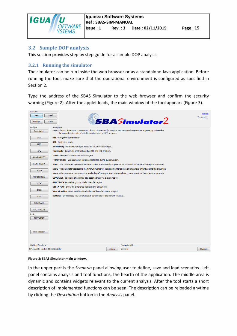
Figure 3: SBAS Simulator main window.
In the upper part is the Scenario panel allowing user to define, save and load scenarios. Left
panel contains analysis and tool functions, the hearth of the application. The middle area is
dynamic and contains widgets relevant to the current analysis. After the tool starts a short
description of implemented functions can be seen. The description can be reloaded anytime
by clicking the Description button in the Analysis panel.

Iguassu Software Systems
Ref : SBAS-SIM-MANUAL
Issue : 1 Rev. : 3 Date : 02/11/2015 Page : 16
In the bottom user can set the working and scenario directory (section 4.6). Working
directory is a folder in the hard disk, where temporary and final results are stored. By default
the folder is set to user home directory.
3.3 Constellations and satellites
DOP configuration can be managed by clicking the DOP button in the Analysis panel. The
Description panel is changed to DOP Settings panel, where are all necessary widgets for DOP
analysis.
Constellation Setup panel defines the space segment of the SBAS Simulator. Constellation
can be switched by using the tab at the top (GEO, GPS, GLONASS, GALILEO). A constellation
is used in the simulation, when the Use check box is selected. Particular satellites can be
selected or deselected as well. Default values are used for the purpose of this simulation.
Detailed space segment configuration can be found in section 4.1.
3.4 Simulation time and area
The Time panel shows the simulation length and the time step. Simulation length is the total
length of the simulation and time step is the interval within 2 closest computations. Keep the
default settings (24h simulation with 10-minute step). Time settings are described in section
4.4.
Simulation area is the area where the analysis is performed. It can be set to a region or a
point. For the purpose of this simulation, the default area shall be kept (ECAC square region
with the grid step of 5°). Information about geographical area settings can be found in
section 4.2.1.
3.5 DOP options and analysis
In the right part of the DOP Settings panel is the Simulate DOP button. After clicking on it,
the DOP Simulation Settings window appears (Figure 4).
Figure 4: DOP Simulation Settings window.

Iguassu Software Systems
Ref : SBAS-SIM-MANUAL
Issue : 1 Rev. : 3 Date : 02/11/2015 Page : 17
Two types of simulation are implemented: Availability and Statistics. I this example, the DOP
availability will be shown. It computes the percent of time when DOP is bellow availability
limits defined in the DOP Simulation Settings window. Simulation is started by clicking the
OK button. The progress bar appears showing the computational details. First satellite
positions are calculated; later ENU coordinates for each point in the region and finally the
DOP availability.
When finished, the graph with DOP availability results is shown (Figure 5).
Figure 5: HDOP availability for ECAC region.
Buttons in the upper-left part of the graph are used to switch among HDOP, VDOP, GDOP,
PDOP and TDOP results.
More information about DOP analysis can be found in section 5.3. Graph features are
detailed in section 6.
4 Settings Before doing any analysis, various parameters and initial conditions shall be set. Initial
settings of the tool are visible after clicking the Settings button in the Scenario panel. There
are more settings specific to each simulation, which are configurable in a separate window
before the analysis starts.

Iguassu Software Systems
Ref : SBAS-SIM-MANUAL
Issue : 1 Rev. : 3 Date : 02/11/2015 Page : 18
4.1 Space segment settings
Space segment defines constellations, satellites and frequencies used in the simulations. The
main window contains the Constellation Setup panel where constellations can be configured
(Figure 6).
Figure 6: Constellation Setup panel.
In the Constellation Setup panel user can define which constellations and satellites will be
used for the simulation and also define new ones. Four constellations are available after
loading the tool: GEO, GPS, GLONASS and GALILEO. Only GEO and GPS are selected as used
for the simulation by default. To switch among constellations, use the tab panel in the upper
part of the window. It is possible to select the whole constellation to be used or not used by
clicking on the Use check box. The Show PRN numbers check box switches between the
satellite name and its PRN number. Individual satellite can be also selected or deselected
from the simulation using the check box next to it.
4.1.1 Satellite settings
Right-clicking on a specific satellite opens the satellite configuration window (Figure 7).
Iguassu Software Systems
Ref : SBAS-SIM-MANUAL
Issue : 1 Rev. : 3 Date : 02/11/2015 Page : 19
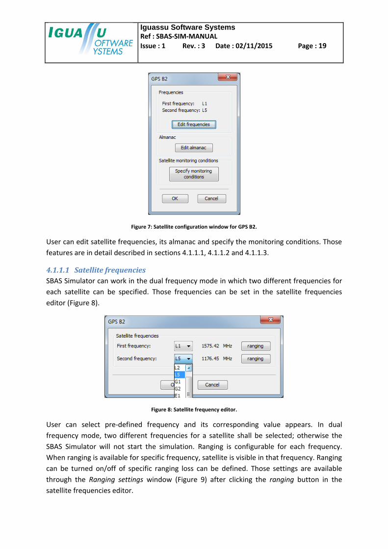
Figure 7: Satellite configuration window for GPS B2.
User can edit satellite frequencies, its almanac and specify the monitoring conditions. Those
features are in detail described in sections 4.1.1.1, 4.1.1.2 and 4.1.1.3.
4.1.1.1 Satellite frequencies
SBAS Simulator can work in the dual frequency mode in which two different frequencies for
each satellite can be specified. Those frequencies can be set in the satellite frequencies
editor (Figure 8).
Figure 8: Satellite frequency editor.
User can select pre-defined frequency and its corresponding value appears. In dual
frequency mode, two different frequencies for a satellite shall be selected; otherwise the
SBAS Simulator will not start the simulation. Ranging is configurable for each frequency.
When ranging is available for specific frequency, satellite is visible in that frequency. Ranging
can be turned on/off of specific ranging loss can be defined. Those settings are available
through the Ranging settings window (Figure 9) after clicking the ranging button in the
satellite frequencies editor.

Iguassu Software Systems
Ref : SBAS-SIM-MANUAL
Issue : 1 Rev. : 3 Date : 02/11/2015 Page : 20
Figure 9: Ranging settings window.
By default the ranging is always available and there is no loss of the satellite signal. User can
define two different types of signal loss: temporary and random. Temporary data loss
specifies time intervals when the ranging is not available (Figure 10). Several time intervals
can be specified. A new interval is added clicking the Add time interval button. Interval is
deleted clicking the red cross next to the value fields. It is also possible to delete all time
intervals through the Delete all intervals button.
Figure 10: Temporary ranging data loss.

Iguassu Software Systems
Ref : SBAS-SIM-MANUAL
Issue : 1 Rev. : 3 Date : 02/11/2015 Page : 21
Random data loss specifies the probability of the signal loss. User specifies the value in
percent (Figure 11). During the simulation the tool decides if the signal will be available or
not based on the integrated random generator.
Figure 11: Random data loss.
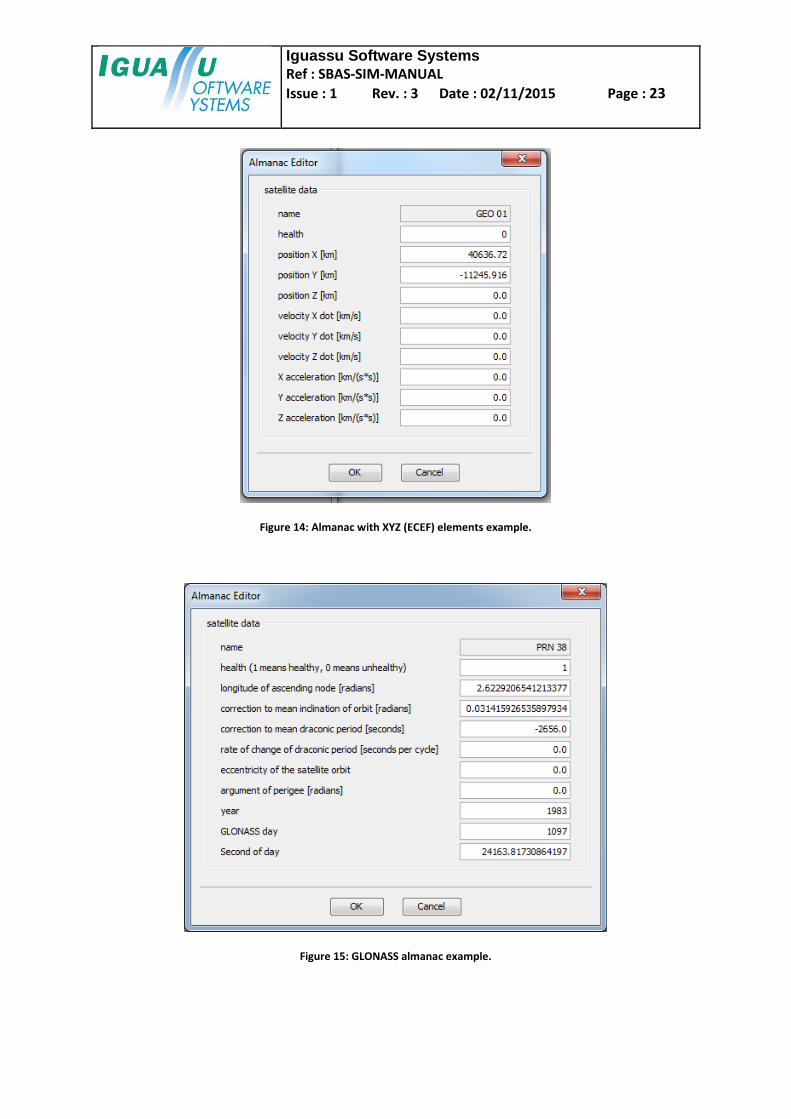
4.1.1.2 Satellite almanacs
SBAS Simulator supports 3 different types of almanacs, one of which has 2 subtypes:
Almanac with Keplerian elements (2 different subtypes)
o with Longitude of Ascending Node of Orbit Plane at Weekly Epoch (LANOPWE
for short)
o with Right Ascension of the Ascending Node (RAAN for short)
Almanac with XYZ (ECEF) elements
GLONASS Almanac
Satellite almanacs can be edited in the Almanac Editor window. Figure 12, Figure 13, Figure
14 and Figure 15 contain examples of Almanac Editor windows for all types of supported
almanacs. Table 4 shows examples of where the values of the fields can be found.

Iguassu Software Systems
Ref : SBAS-SIM-MANUAL
Issue : 1 Rev. : 3 Date : 02/11/2015 Page : 22
Figure 12: Almanac with Keplerian elements with Longitude of Ascending Node of Orbit Plane at Weekly Epoch (LANOPWE) example.
Figure 13: Almanac with Keplerian elements with Right Ascension of the Ascending Node (RAAN) example.
Iguassu Software Systems
Ref : SBAS-SIM-MANUAL
Issue : 1 Rev. : 3 Date : 02/11/2015 Page : 23
Figure 14: Almanac with XYZ (ECEF) elements example.
Figure 15: GLONASS almanac example.

Iguassu Software Systems
Ref : SBAS-SIM-MANUAL
Issue : 1 Rev. : 3 Date : 02/11/2015 Page : 24
Element/field Included in type of
almanac Source example
health Keplerian with LANOPWE, Keplerian with RAAN, XYZ (ECEF)
YUMA almanac
eccentricity
Keplerian with LANOPWE, Keplerian with RAAN
YUMA almanac
semi-major axis [m]
YUMA almanac (SQRT(A) (m 1/2) in the almanac, square root of semi-major axis in the almanac (here the square root is squared))
Longitude of ascending node at weekly epoch [rad]
Keplerian with LANOPWE YUMA almanac (Right Ascen at Week(rad) in the almanac)
Right ascension of ascending node [rad]
Keplerian with RAAN TLE (in degrees in TLE (here in radians))
mean anomaly [rad]
Keplerian with LANOPWE, Keplerian with RAAN
YUMA almanac
orbit inclination [rad] YUMA almanac
argument of perigee [rad] YUMA almanac
toa Week
RINEX 3.02 GNSS Navigation Message File – GPS Data Record (GPS Week # (to go with TOE) in RINEX)
toa SOW
RINEX 3.02 GNSS Navigation Message File – GPS Data Record (Toe Time of Ephemeris in RINEX)
position X [km]
XYZ (ECEF)
RINEX 3.02 GNSS Navigation Message File – SBAS Data Record
position Y [km]
position Z [km]
velocity X dot [km/s] RINEX 3.02 GNSS Navigation Message File – SBAS Data Record (for practical reasons these fields are left 0 when loading from RINEX)
velocity Y dot [km/s]
velocity Z dot [km/s]
X acceleration [km/(s*s)]
Y acceleration [km/(s*s)]
Z acceleration [km/(s*s)]
health (1 means healthy, 0 means unhealthy)
GLONASS
GLONASS almanac (.agl)
longitude of ascending node [radians]
GLONASS almanac (.agl; Lam in the almanac, in semi-cycles in the almanac (here in radians))
correction to mean inclination of orbit [radians]
GLONASS almanac (.agl; dI in the almanac, in semi-cycles in the almanac (here in radians))

Iguassu Software Systems
Ref : SBAS-SIM-MANUAL
Issue : 1 Rev. : 3 Date : 02/11/2015 Page : 25
correction to mean draconic period [seconds]
GLONASS almanac (.agl; dT in the almanac)
rate of change of draconic period [seconds per cycle]
GLONASS almanac (.agl; dTT in the almanac)
eccentricity of the satellite orbit
GLONASS almanac (.agl; E in the almanac)
argument of perigee [radians] GLONASS almanac (.agl; w in the almanac, in semi-cycles in the almanac (here in radians))
year GLONASS almanac (.agl)
GLONASS day GLONASS almanac (.agl; made using day, month and year from the almanac)
Second of day GLONASS almanac (.agl) Table 4: Almanac fields and examples of sources of values.
4.1.1.3 Satellite monitoring conditions
Each satellite in the SBAS Simulator can have two monitoring states: monitored and not
monitored. When the satellite is monitored, it is used for the SBAS Simulation otherwise not.
Monitoring depends on the number of actual visible RIMS. It also depends on satellite
ranging and the RIMS availability. When a satellite signal is lost or RIMS is not available, the
RIMS for that satellite is not visible even if it is geometry shows the opposite. RIMS have
several types (A, B, C, D, E and F). Satellite is considered monitored when it sees at least
specific number of each RIMS type. This configuration is done through the Monitor settings
window as shown in Figure 16.
Figure 16: Monitor settings window for satellite B2.

Iguassu Software Systems
Ref : SBAS-SIM-MANUAL
Issue : 1 Rev. : 3 Date : 02/11/2015 Page : 26
4.1.2 Adding and removing satellite from a constellation
By pressing the Add a satellite button a satellite can be added into the constellation. By
pressing Remove selected satellites, all selected satellites are removed from the constellation.
Both of these buttons can be found in the Constellation Setup panel (Figure 6).
4.1.2.1 Adding a satellite to the constellation
Each constellation can have a limited number of satellites. Four default constellations and
custom constellations have different limits for the maximum number of satellites (see Table
5). Once the maximum number of satellites has been reached, no new satellites can be
added to the constellation before some of the satellites are removed first. The total number
of satellites in all custom constellations cannot be more than 63.
Constellation Maximum number of
satellites Available PRNs
GEO 40 120 – 159 (both inclusive)
GPS
37
1 – 37 (both inclusive)
GLONASS 38 – 74 (both inclusive)
Galileo 75 – 111 (both inclusive)
Custom constellation 40 in one constellation,
63 in total in all constellations
112 – 119 (both inclusive), 160 – 214 (both inclusive)
Table 5: Maximum number of satellites for different constellations and available PRNs.
Constellation Constrains for satellite names
GEO
Length of the name of the satellite must be at least 1 character and at most 10 characters.
GLONASS
Galileo
Custom constellation
GPS (when orbit slots are available)
Name must be in the format XYZ or XY, where X is a letter, an element from {‘A’, ‘B’, ‘C’, ‘D’, ‘E’, ‘F’}, Y is a
number between 1 and 9 (both inclusive), Z is a letter, an element from {‘A’, ‘F’}. Examples: A6, D2F, F1A.
For a particular pair (X, Y) it is not possible to have an XYZ (for any Z) and XY satellite in the constellation at
the same time. It is possible to have both XYZ satellites in the constellation though. Example: When A6F is in the constellation, A6 cannot be added, A6A
can be added however. Table 6: Names of satellites rules.
Iguassu Software Systems
Ref : SBAS-SIM-MANUAL
Issue : 1 Rev. : 3 Date : 02/11/2015 Page : 27
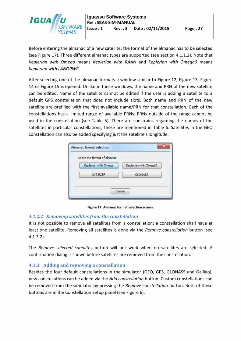
Before entering the almanac of a new satellite, the format of the almanac has to be selected
(see Figure 17). Three different almanac types are supported (see section 4.1.1.2). Note that
Keplerian with Omega means Keplerian with RAAN and Keplerian with Omega0 means
Keplerian with LANOPWE.
After selecting one of the almanac formats a window similar to Figure 12, Figure 13, Figure
14 or Figure 15 is opened. Unlike in those windows, the name and PRN of the new satellite
can be edited. Name of the satellite cannot be edited if the user is adding a satellite to a
default GPS constellation that does not include slots. Both name and PRN of the new
satellite are prefilled with the first available name/PRN for that constellation. Each of the
constellations has a limited range of available PRNs. PRNs outside of the range cannot be
used in the constellation (see Table 5). There are constrains regarding the names of the
satellites in particular constellations, these are mentioned in Table 6. Satellites in the GEO
constellation can also be added specifying just the satellite’s longitude.
Figure 17: Almanac format selection screen.
4.1.2.2 Removing satellites from the constellation
It is not possible to remove all satellites from a constellation; a constellation shall have at
least one satellite. Removing all satellites is done via the Remove constellation button (see
4.1.3.2).
The Remove selected satellites button will not work when no satellites are selected. A
confirmation dialog is shown before satellites are removed from the constellation.
4.1.3 Adding and removing a constellation
Besides the four default constellations in the simulator (GEO, GPS, GLONASS and Galileo),
new constellations can be added via the Add constellation button. Custom constellations can
be removed from the simulator by pressing the Remove constellation button. Both of these
buttons are in the Constellation Setup panel (see Figure 6).
Iguassu Software Systems
Ref : SBAS-SIM-MANUAL
Issue : 1 Rev. : 3 Date : 02/11/2015 Page : 28
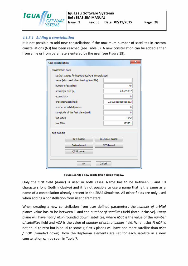
4.1.3.1 Adding a constellation
It is not possible to add new constellations if the maximum number of satellites in custom
constellations (63) has been reached (see Table 5). A new constellation can be added either
from a file or from parameters entered by the user (see Figure 18).
Figure 18: Add a new constellation dialog window.
Only the first field (name) is used in both cases. Name has to be between 3 and 10
characters long (both inclusive) and it is not possible to use a name that is the same as a
name of a constellation already present in the SBAS Simulator. All other fields are only used
when adding a constellation from user parameters.
When creating a new constellation from user defined parameters the number of orbital
planes value has to be between 1 and the number of satellites field (both inclusive). Every
plane will have nSat / nOP (rounded down) satellites, where nSat is the value of the number
of satellites field and nOP is the value of number of orbital planes field. When nSat % nOP is
not equal to zero but is equal to some x, first x planes will have one more satellite than nSat
/ nOP (rounded down). How the Keplerian elements are set for each satellite in a new
constellation can be seen in Table 7.

Iguassu Software Systems
Ref : SBAS-SIM-MANUAL
Issue : 1 Rev. : 3 Date : 02/11/2015 Page : 29
Keplerian element of a new satellite (see Figure 12)
value for i-th satellite in the new constellation (see Figure 18)
PRN i-th available PRN not already used in a custom constellation (see Table 5)
name
XXX YY where
XXX is the first three letters of the constellation name, always upper case (even if the name of the constellation is not in upper case)
YY is i formatted to 2 characters (e.g. if i is 4, YY would be 04)
Example:
constellation name is MyConstellation
i is 7
name of the satellite would be MYC 07
health 0
eccentricity value of field eccentricity
semi-major axis [m] value of the field semi-major axis [m]
Longitude of ascending node at weekly epoch [rad]
raFirst + 2*pi*j / nPlanes where
raFirst is the value of the field Longitude of the first plane [rad]
j is the number of the satellite’s plane (for 1st plane j is 0)
nPlanes is the value of the field number of orbital planes
mean anomaly [rad]
2*pi*k / sIP[j] Where
k is the number of satellite in the plane (1st satellite in the plane has k equal to 0)
sIP[j] is the number of satellites in plane j, where plane j contains the satellite i
orbit inclination [rad] value of field orbit inclination [rad]
argument of perigee [rad] 0
toa Week value of field toa Week
toa SOW value of field toa SOW Table 7: Keplerian element values for a satellite in a new constellation added from user parameters.
Iguassu Software Systems
Ref : SBAS-SIM-MANUAL
Issue : 1 Rev. : 3 Date : 02/11/2015 Page : 30
When adding a new constellation from a file, user shall choose the base constellation. Unlike
rewriting an existing default constellation (see section 4.1.5), the loaded constellation is put
in a new tab in the Constellation setup panel (see Figure 6). When based on GPS, loading of a
new constellation will not change the Simulation start time (see section 4.4), unlike rewriting
the default GPS constellation (see section 4.1.5.2). Satellites’ names and PRNs are set
according to rules in Table 7 even if PRNs or names are available (through RINEX or TLE files).
Loading fails if a file contains too many satellites (see Table 5).
When loading a new constellation from a QZSS based file, the file has to be a RINEX version
3.02 or 2.12. RINEX 3.02 may be mixed, in that case only QZSS satellites are loaded from it. If
a RINEX contains multiple instances of the same QZSS satellite, the instance with newest GPS
Week and Time of Ephemeris is loaded. QZSS entries in a RINEX file contain information used
to create almanacs of type Keplerian with LANOPWE.
4.1.3.2 Removing a constellation
Only custom constellations can be removed. When a custom constellation is present in the
simulator, pressing the Remove constellation button will open a dialog window where the
user can choose a constellation to be deleted.
4.1.4 Setting the constellation to the default state
A constellation can be reset to its default values using the Default button in the Constellation
Setup panel (see Figure 6). For a default constellation (GEO, GPS, GLONASS or Galileo)
default values are those set when the simulator has been launched. For a custom
constellation default values are those set when the constellation was added to the simulator.
When the reset constellation σ value is checked (see Figure 19) sigma values are reset to the
original state (see 4.5.1).
When reset constellation data is checked all parameters under Constellation settings at the
top of Constellation Setup panel (see Figure 6) are reset to defaults. Also the composition of
the constellation is reset: all satellites removed from the original constellation are restored
and all satellites added on top of the original constellation are removed. Also all settings of
each satellite (see section 4.1.1) are reset to default.

Iguassu Software Systems
Ref : SBAS-SIM-MANUAL
Issue : 1 Rev. : 3 Date : 02/11/2015 Page : 31
Figure 19: Default constellation parameters dialog.
When neither of the checkboxes is checked and OK is pressed, the effect is the same as
pressing Cancel. A warning window may appear informing that the ephemeris time of the
constellation has been changed as a result of resetting the constellation to default values.
4.1.5 Constellation source
Each of the four default constellations (GEO, GPS, GLONASS and Galileo) can be overwritten.
By pressing the Constellation source button in the Constellation Setup panel (see Figure 6) it
is possible to select the source of the default constellation.
4.1.5.1 Source of GEO constellation
In the GEO Constellation window (see Figure 20) four different sources of GEO constellation
can be chosen:
GEO nominal constellation
GEO constellation decoded from an MT17 message
GEO constellation from a RINEX file
GEO constellation from a TLE file
Figure 20: GEO constellation source window.

Iguassu Software Systems
Ref : SBAS-SIM-MANUAL
Issue : 1 Rev. : 3 Date : 02/11/2015 Page : 32
When loading from MT17, satellite names are set to generic GEO XX, where XX is a number
starting from 01. Only the X, Y and Z coordinates and the PRN are taken from the message,
other information, like the velocity, is ignored and set to 0 for all dimensions and for all
satellites.
TLE files used for loading a GEO constellation have to contain on the 0th line the satellite
name and the PRN. An example of such a record with name and PRN both on the 0th line can
be seen in Figure 21. If the TLE file contains multiple instances of the same satellite (satellite
is identified by its PRN), only the first record is taken and all subsequent all ignored. TLE files
don’t contain information about a satellite’s health, health of all satellites loaded from a TLE
thus have their health set to 0. Almanacs created for the satellites from data in a TLE file are
Keplerian with RAAN (see 4.1.1.2).
Figure 21: An example of a record in a TLE file containing both the name and the PRN of a satellite.
RINEX GNSS Navigation Message Files with GEO satellites (named SBAS satellites in RINEX)
contain data about GEO satellites from which XYZ (ECEF) almanacs are created (see 4.1.1.2).
Only RINEX 3, 3.01 and 3.02 are supported when loading GEO satellites. The Satellite System
(included in the header of a RINEX file) can be either S (SBAS Payload) or M (Mixed). For
mixed satellite system, only GEO satellites are loaded from a RINEX file. Acceleration and
velocity in the RINEX are ignored for all dimensions and are set to 0 for each satellite. When
a RINEX file contains multiple records of the same satellite, the record with the newest Time
of Clock is loaded. However that time is not loaded from the RINEX, because the XYZ (ECEF)
almanac does not contain information about the time (see Figure 14). Instead the ephemeris
time of GEO is internally set to the middle of the simulation. PRN of a satellite is created by
adding 100 to satellite number from RINEX. Satellite names are set to GEO XX the same way
as in the case of loading the MT17.
4.1.5.2 Source of GPS Constellation
In the GPS Constellation window (see Figure 22) seven different sources of GPS constellation
can be chosen:
GPS current constellation
GPS nominal constellation (SPS 2008)
GPS expandable constellation (SPS 2008)
Load from YUMA file
Load from SEM file
Load from RINEX file

Iguassu Software Systems
Ref : SBAS-SIM-MANUAL
Issue : 1 Rev. : 3 Date : 02/11/2015 Page : 33
Download from the internet
Figure 22: GPS constellation source window.
Current constellation is loaded from the latest YUMA almanac on the internet. Simulation
start time (see 4.4) is also changed to the current time when loading the latest YUMA
almanac.
When loading from a local YUMA or SEM file, satellite names (slots) are disabled (only PRNs
can be viewed). YUMA and SEM file contain almanacs of satellites in Keplerian with
LANOPWE format (see 4.1.1.2). GPS week number rollover is used because the GPS week
contained in a YUMA or SEM file is modulated by 1024. Thus week number rollover set to 1
will result in 1024 being added to the week from the YUMA/SEM file to create the real GPS
week. Simulation start time (see 4.4) is changed to the time of the 1st satellite that was
loaded from the file.
Loading a GPS constellation from a local RINEX is possible for RINEX version 2.11, 2.12, 3,
3.01, 3.02. For RINEX 3.xx the RINEX GNSS Navigation Message File Header’s Satellite System
can be GPS or Mixed. When the header is mixed, only GPS satellites are loaded from the
RINEX file. When the RINEX file contains multiple records with the same satellite, the record
with the newest GPS Week and Time of Ephemeris is loaded; all other records of the same
satellite are ignored. RINEX with GPS satellites contain data for almanacs in the Keplerian
with LANOPWE format (see 4.1.1.2). As with loading a GPS constellation from a local YUMA
or SEM file, satellite names (slots) are disabled if the GPS constellation is loaded from a local

Iguassu Software Systems
Ref : SBAS-SIM-MANUAL
Issue : 1 Rev. : 3 Date : 02/11/2015 Page : 34
RINEX file. Simulation start time is also changed in a similar way as in the case of loading the
YUMA or SEM file.
When loading the GPS constellation from the internet a YUMA file for the specified day is
downloaded. The simulation start time (see 4.4) is changed to 0:00:00 UTC of that day.
4.1.5.3 Source of GLONASS Constellation
In the GLONASS constellation window (see Figure 23) three different sources of the
GLONASS constellation can be chosen:
GLONASS current constellation
GLONASS nominal constellation
Load from .agl file
Figure 23: GLONASS Constellation source window.
Current constellation is loaded from the current .agl almanac on the internet. Almanacs of
the loaded satellites are in GLONASS almanac format (see 4.1.1.2).
When loading from a local .agl file, PRN of a satellite is created by taking the number of the
spacecraft (included in the .agl file) and adding 37 to it. Thus a satellite from the .agl file with
spacecraft number equal to 1 will get a PRN equal to 38. When an .agl file contains multiple
records of the same satellite (from different times), only the first record of such a satellite is
loaded. Names of satellites loaded from an .agl file are created using the spacecraft number
from the .agl file: every satellite has a name equal to GLO XX, where XX is the spacecraft
number in two digit format. Thus, for example, a satellite with spacecraft number 6 will be
named GLO 06.
4.1.5.4 Source of Galileo constellation
A Galileo constellation can be loaded from 4 different sources (see Figure 24):
Galileo current constellation

Iguassu Software Systems
Ref : SBAS-SIM-MANUAL
Issue : 1 Rev. : 3 Date : 02/11/2015 Page : 35
Galileo nominal constellation
Galileo expandable constellation
Galileo IOV 4 satellites
Figure 24: Galileo constellation source window
Current constellation is loaded from a RINEX file on the internet. PRNs of the satellites are
created by adding 74 to the satellite number from the RINEX file. Thus a Galileo satellite in a
RINEX file with satellite number 11 will have its PRN equal to 85. Names of the satellites are
in the format EXX, where XX is the satellite number from the RINEX file. If a RINEX file
contains multiple records of the same satellite, the records with the newest GAL Week and
Time of Ephemeris is loaded. Almanacs of the loaded satellites are in the Keplerian with
LANOPWE format (see 4.1.1.2).
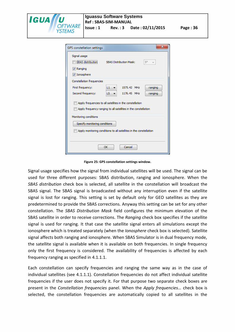
4.1.6 Constellation settings
Each constellation has specific settings that define general characteristics and can also have
effect on individual satellites. The Constellation Settings window (Figure 25) is opened after
clicking the Constellation settings button in the Constellation Setup panel (Figure 6).
Iguassu Software Systems
Ref : SBAS-SIM-MANUAL
Issue : 1 Rev. : 3 Date : 02/11/2015 Page : 36
Figure 25: GPS constellation settings window.
Signal usage specifies how the signal from individual satellites will be used. The signal can be
used for three different purposes: SBAS distribution, ranging and ionosphere. When the
SBAS distribution check box is selected, all satellite in the constellation will broadcast the
SBAS signal. The SBAS signal is broadcasted without any interruption even if the satellite
signal is lost for ranging. This setting is set by default only for GEO satellites as they are
predetermined to provide the SBAS corrections. Anyway this setting can be set for any other
constellation. The SBAS Distribution Mask field configures the minimum elevation of the
SBAS satellite in order to receive corrections. The Ranging check box specifies if the satellite
signal is used for ranging. It that case the satellite signal enters all simulations except the
ionosphere which is treated separately (when the Ionosphere check box is selected). Satellite
signal affects both ranging and ionosphere. When SBAS Simulator is in dual frequency mode,
the satellite signal is available when it is available on both frequencies. In single frequency
only the first frequency is considered. The availability of frequencies is affected by each
frequency ranging as specified in 4.1.1.1.
Each constellation can specify frequencies and ranging the same way as in the case of
individual satellites (see 4.1.1.1). Constellation frequencies do not affect individual satellite
frequencies if the user does not specify it. For that purpose two separate check boxes are
present in the Constellation frequencies panel. When the Apply frequencies… check box is
selected, the constellation frequencies are automatically copied to all satellites in the

Iguassu Software Systems
Ref : SBAS-SIM-MANUAL
Issue : 1 Rev. : 3 Date : 02/11/2015 Page : 37
constellation. When the Apply frequency ranging… check box is selected, the constellation
frequency ranging settings are automatically copied to all satellites in the constellation.
Constellation also specifies monitoring conditions the same way as for individual satellites
(see 4.1.1.3). If the Apply monitoring conditions… check box is selected, constellation
monitoring conditions will be also copied to all satellites in the constellation.
4.1.7 Frequency mode and frequency values
SBAS Simulator main window contains Frequency panel where frequency mode and
individual frequency values can be set (Figure 26).
Figure 26: Frequency panel.
SBAS Simulator can run in two modes. By default, the single frequency mode is used.
Satellite frequencies are treated separately and analysis equations take into account the
dual frequency solution. In the single frequency mode only the first satellite frequency is
used for the simulation.
SBAS Simulator contains several different frequencies: L1, L2, L5, G1, G2, E1, E6, E5a and E5b.
Each frequency has specific frequency value which can be changed by the user (Figure 27).
Figure 27: Frequency values editor.
Iguassu Software Systems
Ref : SBAS-SIM-MANUAL
Issue : 1 Rev. : 3 Date : 02/11/2015 Page : 38
Frequency values affect the solution in the dual frequency mode through the dual frequency
factor as defined in equation (8). In the single frequency mode, frequency value affects only
the Diono parameter in ionospheric computation.
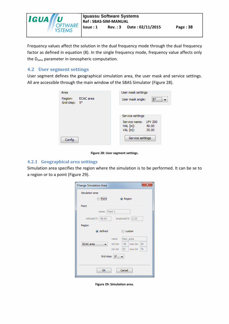
4.2 User segment settings
User segment defines the geographical simulation area, the user mask and service settings.
All are accessible through the main window of the SBAS Simulator (Figure 28).
Figure 28: User segment settings.
4.2.1 Geographical area settings
Simulation area specifies the region where the simulation is to be performed. It can be se to
a region or to a point (Figure 29).
Figure 29: Simulation area.

Iguassu Software Systems
Ref : SBAS-SIM-MANUAL
Issue : 1 Rev. : 3 Date : 02/11/2015 Page : 39
For the point simulation user specifies the coordinates which are set to Paris by default.
When region simulation is chosen, it is possible to select region from a predefined list or
define a custom region. Predefined regions are: ECAC area, ENP, Africa, Europe and Africa,
North America, Japan, India, Russia and World.
ECAC area is set as default. For the custom region, user defines a region name and a border.
Parameter min lon is the longitude where simulation starts and then it goes to the east until
it reaches the max lon, where it stops. Southern border of the simulation area is bounded by
min lat and northern by max lat. Parameter Grid step is the distance (in longitude or latitude)
between 2 closest points in the area. Available values for grid step are 0.5°, 1°, 2.5°, 5°, 10°,
15° and 30°. The default value is 5°. The larger the region and the lower the grid step, the
more time the simulator needs to perform an analysis.
4.2.2 User mask settings
User mask angle defines the minimal elevation below which the satellite will not be used.
Available values are 2°, 5°, 10°, 15° and 30°. The default value is 5°.
4.2.3 Service settings
Service settings (Figure 30) have impact on availability and continuity analyses. Several
services are defined: AVPI, AVPII, CATI, LPV200 and NPA. They specify the HAL and VAL. User
can also define its custom services.
Figure 30: Service settings.
4.3 Ground segment settings
Ground segment consist of various RIMS distributed over the simulated region. The RIMS
panel (Figure 31) is accessible through the main window of the SBAS Simulator. Clicking the
RIMS location map button opens a global view of selected and available RIMS. Other two
buttons allow selecting defined RIMS (4.3.1) and the RIMS error distribution (4.3.4).

Iguassu Software Systems
Ref : SBAS-SIM-MANUAL
Issue : 1 Rev. : 3 Date : 02/11/2015 Page : 40
Figure 31: RIMS panel.
4.3.1 RIMS selection
RIMS selection window (Figure 32) shows all defined RIMS together with a check box. When
the check box is selected, RIMS is used in the simulation, otherwise not. Stations are
grouped into RIMS networks, which collect RIMS over similar geographical area. By default,
the following RIMS networks are present: EGNOS, MEDA, East of Europe, Africa A and B,
Africa C, MIDAN, WAAS, additional RIMS and user defined RIMS. User defined RIMS serve for
defining custom RIMS. After clicking the Define RIMS button, user specifies the RIMS name
and its coordinates.
Figure 32: RIMS selection window.

Iguassu Software Systems
Ref : SBAS-SIM-MANUAL
Issue : 1 Rev. : 3 Date : 02/11/2015 Page : 41
4.3.2 RIMS configuration
Each RIMS can be configured separately. The RIMS configuration window (Figure 33) is
opened after right clicking on a particular station. At the top is displayed RIMS information
and below the configuration panel containing settings for each of the RIMS types (A, B, C, D,
E and F). If the RIMS type is selected, it is active for the simulation, otherwise not. Note that
RIMS types are also part of satellite monitoring conditions (4.1.1.3). RIMS type configuration
window (Figure 34) opens after clicking the Configure button next to the RIMS type. RIMS
type configuration can be divided in RIMS data loss (4.3.2.1), RIMS data availability (4.3.2.2)
and RIMS error bounds (4.3.2.3).
Figure 33: RIMS configuration window.

Iguassu Software Systems
Ref : SBAS-SIM-MANUAL
Issue : 1 Rev. : 3 Date : 02/11/2015 Page : 42
Figure 34: RIMS type configuration window.
4.3.2.1 RIMS data loss
RIMS data loss follows the same idea and same settings as ranging data loss (4.1.1.1). When
RIMS is lost, it is not visible by the satellite and cannot be used for satellite monitoring and
for the IPP computation.
4.3.2.2 RIMS data availability
RIMS availability is similar to RIMS data loss. When RIMS is set as not available, it is not seen
by the satellite and is not used for IPP computation. RIMS unavailability is set by a local mask
and by local time constraints. RIMS elevation mask specifies the local horizon. A RIMS can be
seen by a satellite only when it is above the local horizon. By default the horizon is set to 5°.
It is possible to add more complex horizons through the RIMS elevation settings window
(Figure 35).

Iguassu Software Systems
Ref : SBAS-SIM-MANUAL
Issue : 1 Rev. : 3 Date : 02/11/2015 Page : 43
Figure 35: RIMS elevation mask.
RIMS local time unavailability is set through the RIMS local time unavailability window
(Figure 36). By default, no unavailability periods are defined. The specified time is a local
time for the given RIMS, which is computed from the station longitude. RIMS can be seen by
a satellite only when a satellite is above the RIMS horizon and the station is available at the
given time.
Figure 36: RIMS local time unavailability window.

Iguassu Software Systems
Ref : SBAS-SIM-MANUAL
Issue : 1 Rev. : 3 Date : 02/11/2015 Page : 44
4.3.2.3 RIMS error bounds
RIMS error bounds define the error contribution to the overall satellite error. More details
on the algorithm can be found in [RD2]. By default RIMS is treated as a fault free receiver
with no error contribution. Errors are divided in the interference, noise for MEO, noise for
GEO, multipath and troposphere. User can specify all error contributions. Troposphere and
multipath errors are defined in [RD3]. Noise errors are specified just for a single frequency
solution. For dual frequency solution the value is multiplied by appropriate dual frequency
factor (2.59 for standard L1 and L5). The equation (8) gives details on computing the dual
frequency factor for any frequency combination.
4.3.2.4 RIMS global configuration
In the RIMS configuration window (Figure 33) there is the Configure button next to the
“Global configuration” text. After clicking the button user can configure the RIMS data loss,
availability and error bounds that are not specific to some RIMS type. Those settings can be
applied to all RIMS types if the appropriate check box is selected at the bottom. For example
the same horizon can be easily copied to all RIMS types.
4.3.3 RIMS network configuration
Apart from a global configuration of specific RIMS, it is also possible to globally configure
RIMS from one network. Each RIMS network panel contains a small “c” button that opens a
global configuration window. It contains the same configuration fields as individual station.
At the bottom is a checkbox that makes a copy of the global settings to all RIMS in the
network. This way the user can easily modify a value that is the same for all RIMS. It is
recommended to do first the global network configuration, then the global RIMS
configuration (4.3.2.4) and finally configuration for each RIMS type.
4.3.4 RIMS error distribution
RIMS error distribution specifies the algorithm how particular RIMS errors are applied to the
overall satellite error. It is possible to select between the equal and weighted error
distribution. Details on the algorithm can be found in [RD2].
Figure 37: RIMS error distribution.

Iguassu Software Systems
Ref : SBAS-SIM-MANUAL
Issue : 1 Rev. : 3 Date : 02/11/2015 Page : 45
4.4 Time settings
In the SBAS Simulator main window is the Time panel which shows the simulation length and
the simulation time step. The simulation length is the total length of the simulation.
Simulation time step specifies the interval between two consecutive simulations. Those
values can be set in the Time Configuration window (Figure 38).
Figure 38: Time configuration.
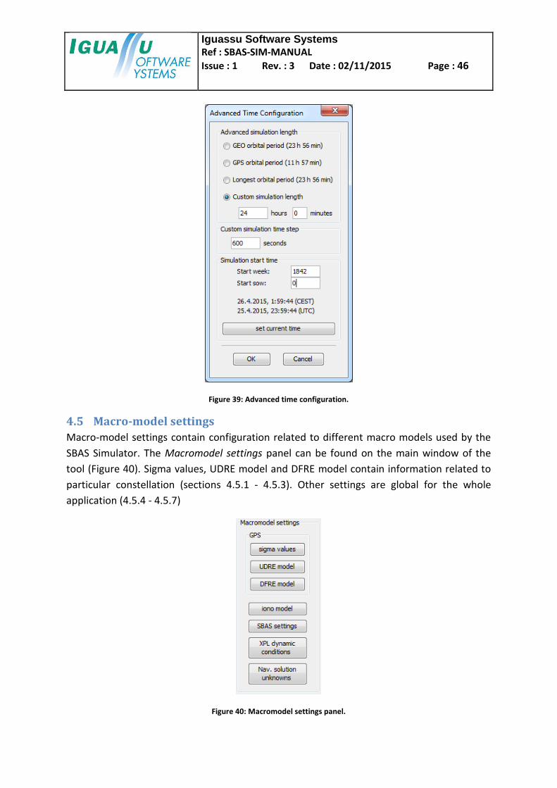
Advanced time settings (Figure 39) can be opened by clicking on the Advanced button. User
can define simulation length based on orbital period of satellites in constellations or set the
custom simulation length. Simulation time step is also configurable. Finally the start
simulation time can be specified filling the GPS week and SOW fields. The start time is also
displayed in local time and in UTC. When the real satellite ephemeris is used, it is the user
responsibility to set the correct start time of the simulation.
Iguassu Software Systems
Ref : SBAS-SIM-MANUAL
Issue : 1 Rev. : 3 Date : 02/11/2015 Page : 46
Figure 39: Advanced time configuration.
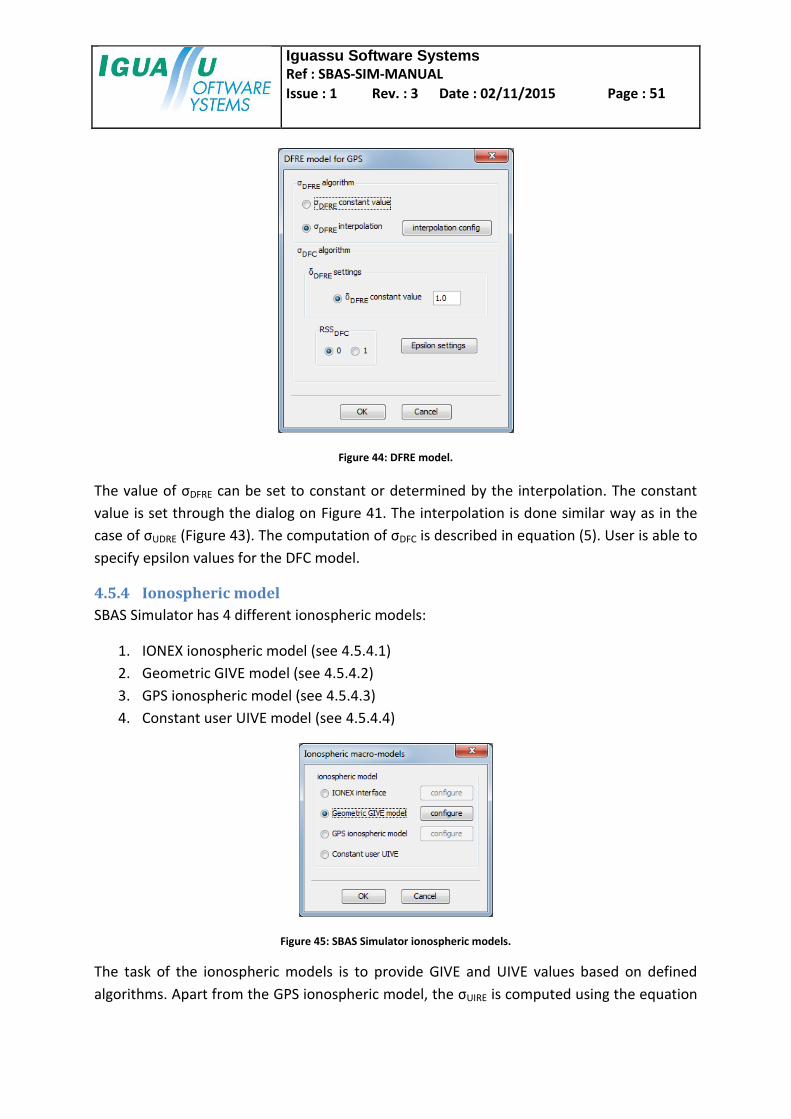
4.5 Macro-model settings
Macro-model settings contain configuration related to different macro models used by the
SBAS Simulator. The Macromodel settings panel can be found on the main window of the
tool (Figure 40). Sigma values, UDRE model and DFRE model contain information related to
particular constellation (sections 4.5.1 - 4.5.3). Other settings are global for the whole
application (4.5.4 - 4.5.7)
Figure 40: Macromodel settings panel.

Iguassu Software Systems
Ref : SBAS-SIM-MANUAL
Issue : 1 Rev. : 3 Date : 02/11/2015 Page : 47
4.5.1 Constellation sigma values
Constellation sigma values contain error over bounds related to specific constellation. Figure
41 shows the situation.
Figure 41: Sigma values for GPS.
Following sigma values are defined:
σUDRE – Editable only in single frequency mode and when the UDRE interpolation is
not used (4.5.2).
σDFRE – Editable only in dual frequency mode and when the DFRE interpolation is not
used (4.5.3).
σUIVE – Editable only in single frequency mode and when the constant user UIVE value
is used (4.5.4).
σnoise – Part of the total satellite noise.
σclock – Part of the total satellite noise.
σorbit – Part of the total satellite noise.
σsystem – Overall constellation system error.
4.5.1.1 Satellite error bound for single frequency mode
For the single frequency mode the overall satellite residual is computed as:
, (1)
where:
σi,sf is the total satellite error over bound for single frequency,

Iguassu Software Systems
Ref : SBAS-SIM-MANUAL
Issue : 1 Rev. : 3 Date : 02/11/2015 Page : 48
σi,flt is defined in MOPS [RD3],
σi,UIRE is defined in MOPS [RD3],
σi,air,sf is the air residual for single frequency specified in equation (2),
σi,tropo is defined in MOPS [RD3],
σi,RIMS is the error contribution from RIMS as defined in [RD2],
σi,system is the overall constellation system error (4.5.1).
The σi,air,sf is computed as:
(2)
, (3)
where
σi,multipath is defined in MOPS [RD3],
σi,noise, σi,clock and σi,orbit are part of the total satellite noise (4.5.1).
4.5.1.2 Satellite error bound for dual frequency mode
For the dual frequency mode the overall satellite residual is computed as:
, (4)
where
σi,DFC is the model variance for dual frequency residual error as specified in equation
(5),
σi,iono is the ionospheric residual error for dual frequency services as specified in
equation (6),
σi,air,df is the air residual for double frequency specified in equation (7),
σi,tropo is defined in MOPS [RD3],
σi,RIMS is the error contribution from RIMS as defined in [RD2],
σi,system is the overall constellation system error (4.5.1).
The σi,DFC is computed as:
, (5)
where parameters in the equation are specified in section 4.5.3.

Iguassu Software Systems
Ref : SBAS-SIM-MANUAL
Issue : 1 Rev. : 3 Date : 02/11/2015 Page : 49
The σi,iono is computed as:
, (6)
where Fpp is defined in MOPS [RD3].
The σi,air,df is computed as:
, (7)
where fdual is dual frequency factor defined as:
, (8)
where f1 is the first frequency and f2 is the second frequency. For L1 and L5 the dual
frequency factor is 2.59.
4.5.2 UDRE model
UDRE model specifies how the satellite UDRE is computed. This model is available only in the
single frequency mode. User can select the algorithm for σUDRE computation and also the σflt
algorithm (Figure 42).
Figure 42: UDRE model.
The value of σUDRE can be set to constant or determined by the interpolation. The constant
value is set through the dialog on Figure 41. The interpolation is done in the window on

Iguassu Software Systems
Ref : SBAS-SIM-MANUAL
Issue : 1 Rev. : 3 Date : 02/11/2015 Page : 50
Figure 43. During the interpolation, the σUDRE is set to the value which is based on number of
RIMS that monitor a specific satellite.
Figure 43: Sigma UDRE interpolation.
The computation of σflt is described in MOPS [RD3]. User is able to specify MT27 and epsilon
values for LTC.
4.5.3 DFRE model
DFRE model specifies how the satellite DFRE is computed. This model is available only in the
dual frequency mode. User can select the algorithm for σDFRE computation and also the σDFC
algorithm (Figure 44).
Iguassu Software Systems
Ref : SBAS-SIM-MANUAL
Issue : 1 Rev. : 3 Date : 02/11/2015 Page : 51
Figure 44: DFRE model.
The value of σDFRE can be set to constant or determined by the interpolation. The constant
value is set through the dialog on Figure 41. The interpolation is done similar way as in the
case of σUDRE (Figure 43). The computation of σDFC is described in equation (5). User is able to
specify epsilon values for the DFC model.
4.5.4 Ionospheric model
SBAS Simulator has 4 different ionospheric models:
1. IONEX ionospheric model (see 4.5.4.1)
2. Geometric GIVE model (see 4.5.4.2)
3. GPS ionospheric model (see 4.5.4.3)
4. Constant user UIVE model (see 4.5.4.4)
Figure 45: SBAS Simulator ionospheric models.
The task of the ionospheric models is to provide GIVE and UIVE values based on defined
algorithms. Apart from the GPS ionospheric model, the σUIRE is computed using the equation

Iguassu Software Systems
Ref : SBAS-SIM-MANUAL
Issue : 1 Rev. : 3 Date : 02/11/2015 Page : 52
A-43 of MOPS [RD3]. Ionospheric models are used only in the single frequency mode. In the
dual frequency mode the ionospheric-free solution is used.
4.5.4.1 IONEX model
The IONEX ionosphere model is described in detail in [RD4]. The GIVE computation is based
on a linear function between the turning point and the point at storm conditions:
, (9)
where a is the slope, Dfactor is the degradation factor and m is the offset. If the Dfactor value is
not between the turning point and storm condition, the GIVE is set to constant.
The relation between GIVE and σGIVE is specified by the following equation:
(10)
Degradation factor is computed as:
, (11)
where Dmonitor reflects the spatial distribution of IPPs around and IGP and Diono takes into
account the gradient of total electron content. More details can be found in [RD4].
SBAS Simulator provides detailed configuration of the following model subcomponents (see
also Figure 46):
general ionosphere settings
Dmonitor settings (includes D#IPP and DGEO settings)
Dfactor settings
ionospheric scintillation settings (includes polar and two equator regions); can be
switched off
Diono settings (includes the IONEX file location)

Iguassu Software Systems
Ref : SBAS-SIM-MANUAL
Issue : 1 Rev. : 3 Date : 02/11/2015 Page : 53
Figure 46: IONEX ionospheric model.
The IONEX file must be provided or simulations dependent on the ionosphere will fail. User
is responsible that data in the IONEX file corresponds to the simulation interval.
4.5.4.2 Geometric GIVE model
Geometric model takes into account ionospheric scintillations and spatial distribution of IPPs
around an IGP. When scintillation happens to a particular IPP, this IPP is not present in the
simulation. It is possible to disable scintillation for the simulation. The spatial distribution
(Dmonitor settings) can change a specific IGP to be not monitored. The computation of Dmonitor
can be switched off (only IGP radius is taken into account). The σGIVE value at each IGP is
based on the number of surrounding IPPs. All values can be configured through the
geometric model window (Figure 47).
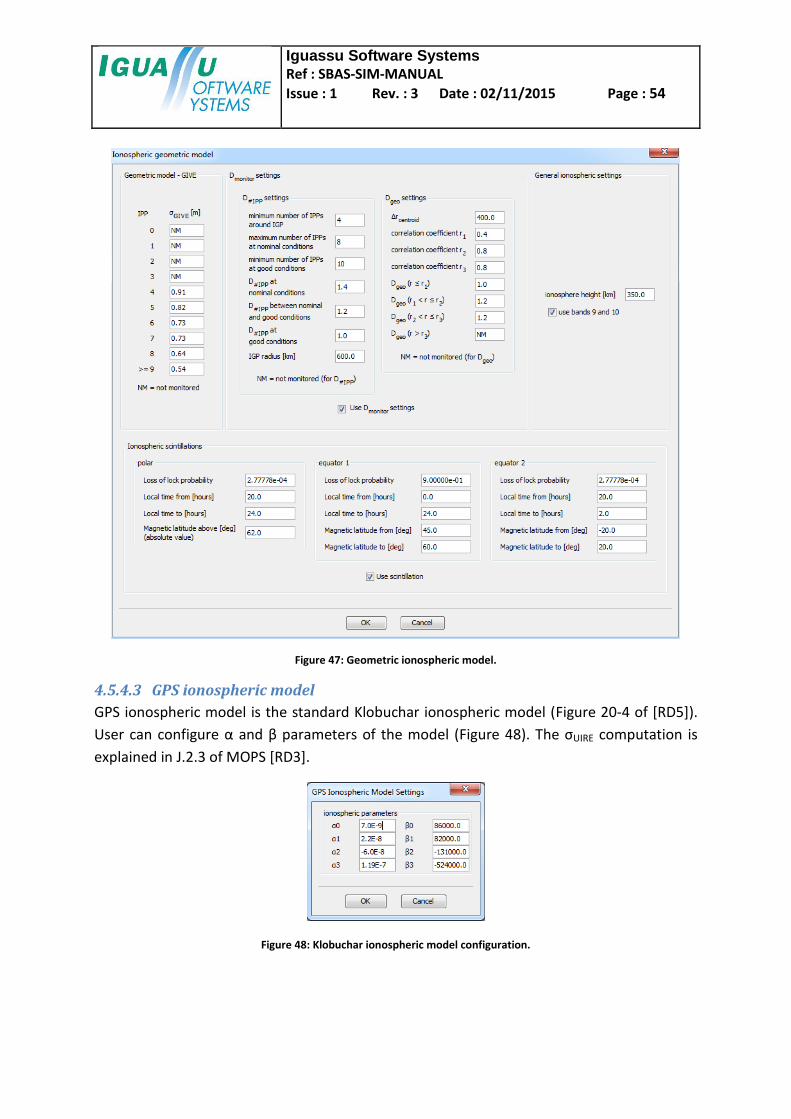
Iguassu Software Systems
Ref : SBAS-SIM-MANUAL
Issue : 1 Rev. : 3 Date : 02/11/2015 Page : 54
Figure 47: Geometric ionospheric model.
4.5.4.3 GPS ionospheric model
GPS ionospheric model is the standard Klobuchar ionospheric model (Figure 20-4 of [RD5]).
User can configure α and β parameters of the model (Figure 48). The σUIRE computation is
explained in J.2.3 of MOPS [RD3].
Figure 48: Klobuchar ionospheric model configuration.

Iguassu Software Systems
Ref : SBAS-SIM-MANUAL
Issue : 1 Rev. : 3 Date : 02/11/2015 Page : 55
4.5.4.4 Constant user UIVE model
When no ionospheric model is used, user provides a constant σUIVE value for each
constellation (Figure 41).
4.5.5 SBAS settings
The total error over bound as specified in equation (1) can be computed using the real data
from internet, local EMS or RINEX files. In this case real SBAS messages are used and they are
processed using MOPS [RD3]. By default, simulation macro models are used. User can switch
to the real data mode in the SBAS Simulation Settings dialog (Figure 49).
Figure 49: SBAS simulation settings.
For the real data simulation it is possible to select between the PA and NPA mode. User is
able to select from different SBAS sources as explained in the following two subsections.
4.5.5.1 Loading SBAS messages from internet
After clicking the Set satellite button user shall choose the augmentation satellite. Internet
SBAS messages are taken from ESA EMS server and only EGNOS satellites are available (PRN
120, PRN 124 and PRN 126).
After confirming the SBAS simulation settings, user has to make sure that the simulation
does not run in the future. SBAS messages are stored on the server as a collection of EMS
files. Each file contains 1-hour record of satellite augmentation broadcast. Every hour new
files are stored on the server with messages from the past hour. Simulation should end at
most an hour before current time so no messages are lost. It is safer to keep the interval
larger. User shall also verify that GPS constellation reflects the real situation for the
simulation time.
EGNOS satellites broadcast augmentations for Europe. The simulation region shall be set to
the ECAC region or to the part of it.
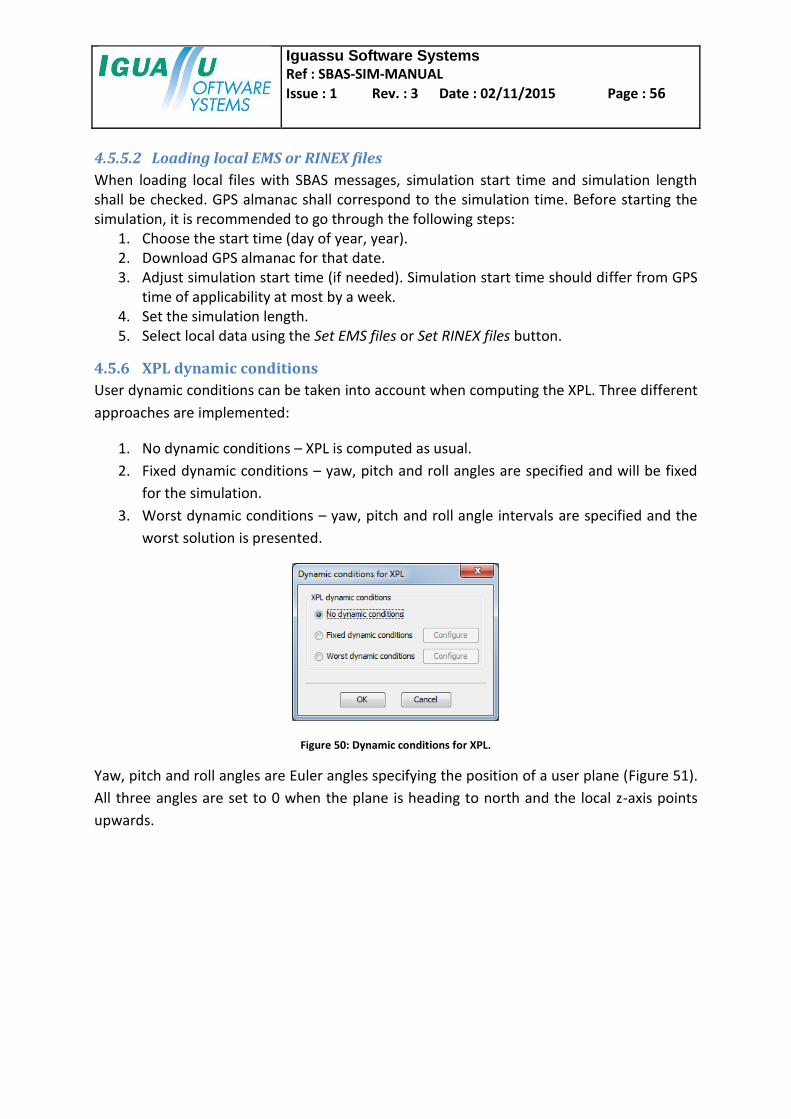
Iguassu Software Systems
Ref : SBAS-SIM-MANUAL
Issue : 1 Rev. : 3 Date : 02/11/2015 Page : 56
4.5.5.2 Loading local EMS or RINEX files
When loading local files with SBAS messages, simulation start time and simulation length shall be checked. GPS almanac shall correspond to the simulation time. Before starting the simulation, it is recommended to go through the following steps:
1. Choose the start time (day of year, year). 2. Download GPS almanac for that date. 3. Adjust simulation start time (if needed). Simulation start time should differ from GPS
time of applicability at most by a week. 4. Set the simulation length. 5. Select local data using the Set EMS files or Set RINEX files button.
4.5.6 XPL dynamic conditions
User dynamic conditions can be taken into account when computing the XPL. Three different
approaches are implemented:
1. No dynamic conditions – XPL is computed as usual.
2. Fixed dynamic conditions – yaw, pitch and roll angles are specified and will be fixed
for the simulation.
3. Worst dynamic conditions – yaw, pitch and roll angle intervals are specified and the
worst solution is presented.
Figure 50: Dynamic conditions for XPL.
Yaw, pitch and roll angles are Euler angles specifying the position of a user plane (Figure 51).
All three angles are set to 0 when the plane is heading to north and the local z-axis points
upwards.

Iguassu Software Systems
Ref : SBAS-SIM-MANUAL
Issue : 1 Rev. : 3 Date : 02/11/2015 Page : 57
Figure 51: Yaw, pitch and roll angles.
The position of the plane defines the local horizon. The local horizon adds additional user
mask to the simulation. Satellite is not visible when it is below the local horizon.
4.5.6.1 Fixed dynamic conditions
Fixed dynamic conditions specify the position of the user plane. The same plane is used for
all user positions. The plane position is defined by yaw, pitch and roll angles which are
configurable (Figure 52).
Figure 52: Fixed dynamic conditions configuration.
Plane Euler angles define the local horizon that affects the visibility of satellites. XPL
computation takes this additional mask into account.
4.5.6.2 Worst dynamic conditions
Worst dynamic conditions move the user plane within the specific interval. User can define
the interval and the moving step for each angle (Figure 53).

Iguassu Software Systems
Ref : SBAS-SIM-MANUAL
Issue : 1 Rev. : 3 Date : 02/11/2015 Page : 58
Figure 53: Worst dynamic conditions configuration.
During the simulation the plane is moving within defined intervals and for each plane
position the XPL is computed. After XPL was computed for all positions, the worst value is
stored. The position of the plane for the worst solution can be different at different user
locations. The simulation can take more time when using the worst dynamic conditions.
4.5.7 Navigation solution unknowns
By default, the system error algorithms use the weighted solution with 4 unknowns as
defined in MOPS [RD3]. When multiple constellations are used, it is possible to make the
weighted solution with 5 unknowns.
Figure 54: Navigation solution unknowns.
The system broadcasts corrections with respect to each constellation system reference time.
The inter constellation time offset and receiver inter system measurement offset is
determined at user level by adding an unknown to equations provided in MOPS [RD3]. When
using the 5 unknowns approach, a reference constellation shall be selected. The observation
matrix then takes the form:
, (12)

Iguassu Software Systems
Ref : SBAS-SIM-MANUAL
Issue : 1 Rev. : 3 Date : 02/11/2015 Page : 59
with ni = 0 if satellite is part of reference constellation and ni=1 if satellite is part of offset
constellation.
To be able to run the simulation with 5 unknowns, at least two different constellations with
ranging must be used.
4.6 Working directory and scenario folder
Working directory is the base directory for storing scenarios. Working directory is set to user
home directory by default and it can be changed clicking the Browse button in the Working
directory panel (Figure 55). Changes are saved to the registry and are loaded each time the
simulator starts.
Figure 55: Working directory.
Working directory contains the scenario directory. Scenario directory stores intermediate
and final SBAS Simulator files. It is the only directory where the tool writes data without
asking the user. It is also the base directory for saving and loading scenarios and images. The
scenario folder can be changed in the Scenario folder panel (Figure 56).
Figure 56: Scenario folder.
4.7 Scenario
Scenario is a collection of all SBAS simulator settings, including all extra user data like
constellations or RIMS. All configuration of SBAS Simulator can be saved to scenario files.
Scenarios can be managed through the Scenario panel.
Figure 57: Scenario panel.
Following buttons are present:
New - Current scenario is erased and all simulator settings return to its default state.
Settings - User can see and change all settings of the tool.
Load - Load existing scenario into the simulator.
Save – Simulator settings are saved to scenario files (*.sce).

Iguassu Software Systems
Ref : SBAS-SIM-MANUAL
Issue : 1 Rev. : 3 Date : 02/11/2015 Page : 60
Scenarios can be saved and loaded through scenario files. Three types of scenario files are
present:
Constellation scenario file – contains all settings related to space segment, all
constellations, satellites, almanacs, frequencies, monitoring conditions, etc.
RIMS scenario file – contains all settings related to ground segment and detailed
RIMS configuration.
Other scenario file – contains all other SBAS Simulator settings that were not covered
by constellation or RIMS scenario files.
Scenario file is a text file, where data are stored in the form of parameter=value or CSV lines.
It is divided into blocks, each starting with a #header and containing settings specific for the
block.
5 Analyses and Tools Analyses and Tools are available through buttons in the left panel of SBAS Simulator.
Description gives short information of implemented functions. After clicking any analysis or
tool button, all important configuration needed by the simulation is shown in the main panel.
Before starting the simulation, required settings shall be checked. Detailed explanation of all
possible settings in the main panel is given in section 4.
Simulation can be performed over a point or a region (see section 4.2.1). Not all simulations
are available for both and some are also restricted only to the World. Ionosphere simulation
is available only for single frequency mode. Table 8 shows the area simulation availability.
Simulation Geographical area Frequency mode
Point Region single Dual
DOP
NSE
XPL
Availability
Continuity
Ionosphere
Monitoring
XDOC
IDOC
ADOC
Coverage (World)
Elevation
Ground Tracks (World)
3D view

Iguassu Software Systems
Ref : SBAS-SIM-MANUAL
Issue : 1 Rev. : 3 Date : 02/11/2015 Page : 61
Sky plot Table 8: Analyses simulation availability.
For each simulation the Simulate X button is presented in the top-right corner of the main
panel. It starts the simulation or opens additional simulation settings.
Simulation intermediate and final results are saved into the simulation files. General
information about simulation files can be found in section 7. Information about specific files
is provided in the following subsections.
5.1 General computations
Several analyses share similar computations that might be performed before the actual
simulation. Those computations include satellite position, vector to satellites, SBAS
distribution, RIMS filtering, satellites monitored, etc.
Following result files can be available after the general computation is finished:
directory file description
sat SatPosition satellite positions
sat Enu vectors from users to satellites; elevation and azimuth of satellites
sat SbasDistribution SBAS distribution mask
sat Ranging satellite ranging on first and second frequency
sat SatSignals availability of satellite signals for ranging and for ionosphere
rims RimsSatPosition azimuth and elevation of satellites at RIMS
rims RimsVisible visible RIMS
rims RimsRanging RIMS types used for ranging
rims RimsMonitored number of RIMS monitored by a satellite
rims RimsCount number of RIMS types seen by a specific satellite
rims RimsSigma2 error over bound produced by each RIMS type for a specific satellite
sat SatSigma2FromRims overall error bound from used RIMS for a specific satellite
sat SatMonitor monitored satellites
sat UdreDfre σUDRE or σDFRE for specific satellite Table 9: Files generated during general computations.
Listed files are generated in a defined order that is depicted on Figure 58. Note that only files
necessary for the next simulation are generated.

Iguassu Software Systems
Ref : SBAS-SIM-MANUAL
Issue : 1 Rev. : 3 Date : 02/11/2015 Page : 62
Figure 58: File hierarchy for general computations.
5.2 Computations of satellite variance (σ)
The overall satellite error variance depends on the frequency mode. When the simulator is
in the single frequency mode, the total variance is computed from equation (1). In dual
frequency mode the equation (4) is used. Inputs for both equations are specified in sections
4.5.1.1 and 4.5.1.2.
Following result files are available after the satellite variance is computed:
directory File description
sat Sigma2 overall satellite variance Table 10: Files generated during the computation of satellite variance.
Before computing the satellite variance, following input files are needed:
Enu file (see Table 9)
SatSigma2FromRims file (see Table 9) – containing the σi,RIMS values
UdreDfre file (see Table 9) – input for computing σi,flt (single frequency) or σi,DFC (dual
frequency)
Sigma2Uive file (see Table 16) – input for computing σi,UIRE (only single frequency)
Figure 59 shows input files needed to compute the satellite variance. Sigma2Uive file is used
only in the single frequency mode.
Figure 59: Input files needed for the generation of the overall satellite error.

Iguassu Software Systems
Ref : SBAS-SIM-MANUAL
Issue : 1 Rev. : 3 Date : 02/11/2015 Page : 63
5.3 DOP
DOP computes dilution of precision, which is represented by:
HDOP
VDOP
GDOP
PDOP
TDOP
DOP Simulation just takes into account the satellite geometry. Satellite monitoring status or
frequency settings has no effect on this simulation. Availability and statistics simulation can
be computed over a point or region. Before the simulation starts, user can configure the
DOP availability limits.
Following files can be generated during the DOP simulation:
directory file description
dop DopValues DOP values for all region points and times
dop DopAvailability DOP availability
dop DopStatistics DOP statistics for a region
dop DopPointStatistics DOP statistics for a point Table 11: Files generated during the DOP simulation.
Figure 60 shows the computational order of DOP files.
Figure 60: Hierarchy of DOP files.
5.3.1 Availability for a point
DOP versus time is plotted for a given point when performing availability over a point (Figure
61). Availability limit is marked by a red horizontal line. In the upper part of the graph it is
possible to see the percentage of time when the XDOP value was below its availability limit.
Use DOP buttons on the left to switch between particular results.
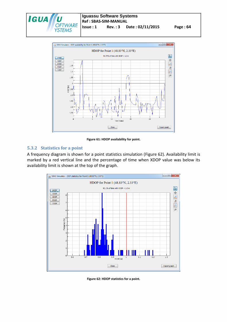
Iguassu Software Systems
Ref : SBAS-SIM-MANUAL
Issue : 1 Rev. : 3 Date : 02/11/2015 Page : 64
Figure 61: HDOP availability for point.
5.3.2 Statistics for a point
A frequency diagram is shown for a point statistics simulation (Figure 62). Availability limit is marked by a red vertical line and the percentage of time when XDOP value was below its availability limit is shown at the top of the graph.
Figure 62: HDOP statistics for a point.

Iguassu Software Systems
Ref : SBAS-SIM-MANUAL
Issue : 1 Rev. : 3 Date : 02/11/2015 Page : 65
5.3.3 Availability for a region
First DOP is computed for each point in the region. Then the percentage of time when DOP value was below its availability limit is calculated. Results are shown in the XDOP region availability graph (Figure 5). In the left part of user can switch between simulation results, show selected RIMS and control graph contours. More information on region graphs is provided in section 6.
5.3.4 Statistics for a region
DOP limits are not necessary and are disabled. As for availability, first DOP is computed for each point in the region. Then the average and maximum DOP values are calculated and shown in the XDOP region statistics graph (Figure 63). In the left part of the graph it is possible to do the same as in the availability graph. Users can also switch between average, maximum and percentile DOP values.
Figure 63: HDOP statistics for region.
5.4 NSE
NSE computes navigation system errors, which are represented by:
HNSE
VNSE
Only satellites that are monitored enter the NSE Simulation. The simulation also depends on the SBAS distribution provided by the augmentation satellite and on the overall sigma error bound as described in 4.5.

Iguassu Software Systems
Ref : SBAS-SIM-MANUAL
Issue : 1 Rev. : 3 Date : 02/11/2015 Page : 66
Following files can be generated during the NSE simulation:
directory file description
nse NseValues NSE values for all region points and times
nse NseAvailability NSE availability
nse NseStatistics NSE statistics for a region
nse NsePointStatistics NSE statistics for a point
nse NsePercentile NSE 95 percentile
nse NseAvailabilityFlags NSE availability flags (0,1) based on the NSE percentile Table 12: Files generated during the NSE simulation.
The computational order of NSE files is shown on Figure 64.
Figure 64: Hierarchy of NSE files.
NSE availability and statistics can be shown for both point and region. When the simulation is run over the region user can also specify the NSE percentile which will be computed over the required area. Simulation results are shown in a similar way like the DOP results. Note that NsePercentile and NseAvailabilityFlags files are inputs for availability and continuity simulations.
5.5 XPL
XPL computes protection levels, which are represented by:
HPL
VPL Only satellites that are monitored enter the XPL Simulation. The simulation also depends on the SBAS distribution provided by the augmentation satellite and on the overall sigma error bound as described in 4.5. Following files can be generated during the XPL simulation:
directory file description
xpl XplValues XPL values for all region points and times

Iguassu Software Systems
Ref : SBAS-SIM-MANUAL
Issue : 1 Rev. : 3 Date : 02/11/2015 Page : 67
xpl XplStatistics XPL statistics for a region
xpl XplPointStatistics XPL statistics for a point Table 13: Files generated during the XPL simulation.
Figure 65 shows the hierarchy of XPL files.
Figure 65: Hierarchy of XPL files.
XPL simulation graphs are similar to NSE statistic graphs.
5.6 Availability
Availability simulation computes the availability for a defined service level (see 4.2.3). There are several criteria to be specified for a system to be available:
1. XPL < XAL: required availability condition - this criteria is always set 2. NSE 95 percentile < NSE limit: availability in accuracy – this criteria is optional (useful
for LPV200) 3. NSE < XPL: integrity criteria – is optional
User can set availability criteria in a dialog window (Figure 66) after the Simulate Availability button is clicked.

Iguassu Software Systems
Ref : SBAS-SIM-MANUAL
Issue : 1 Rev. : 3 Date : 02/11/2015 Page : 68
Figure 66: Availability simulation settings.
Availability computation can be divided in the following steps:
1. Compute XPL values (XplValues file).
2. If NSE is used, compute the NSE values (NseValues file).
3. If the NSE percentile criterion is used, compute the NSE percentile (NsePercentile file)
and then the NSE availability flags (NseAvailabilityFlags file).
4. Use the XPL values and if necessary also the NSE Values and NSE availability flags and
compute the availability flags (AvailabilityFlags file).
5. Use availability flags to compute the availability (Availability file).
Following files can be generated during the availability simulation:
directory file description
avail AvailabilityFlags availability flags (0,1) representing the availability at each point and time
avail Availability overall availability for a region Table 14: Files generated during the availability simulation.
The process of computing availability (continuity) is shown on Figure 67. The arrow A is used
only if the NSE percentile is taken into account. The arrow B is used only if the integrity
criterion is set.

Iguassu Software Systems
Ref : SBAS-SIM-MANUAL
Issue : 1 Rev. : 3 Date : 02/11/2015 Page : 69
Figure 67: Hierarchy of availability and continuity files.
Sample availability simulation for single frequency simulation is shown on Figure 68.
Figure 68: Simulated horizontal availability (24h simulation with 10 minutes time step).
5.7 Continuity
Continuity simulation computes the continuity for a defined service level (see 4.2.3). Before the continuity is computed, the system availability must be known. For that reason the same input criteria are specified as in the case of availability (see Figure 66). From the definition of continuity, the simulation makes sense only with time step of 1 second. After the availability at each moment is known, the simulator first computes the number of continuity events. It is done through a 16 seconds sliding window passing over the simulation interval and counting individual continuity events. After the number of continuity events is known, the continuity risk is computed. More details can be found in [RD6].
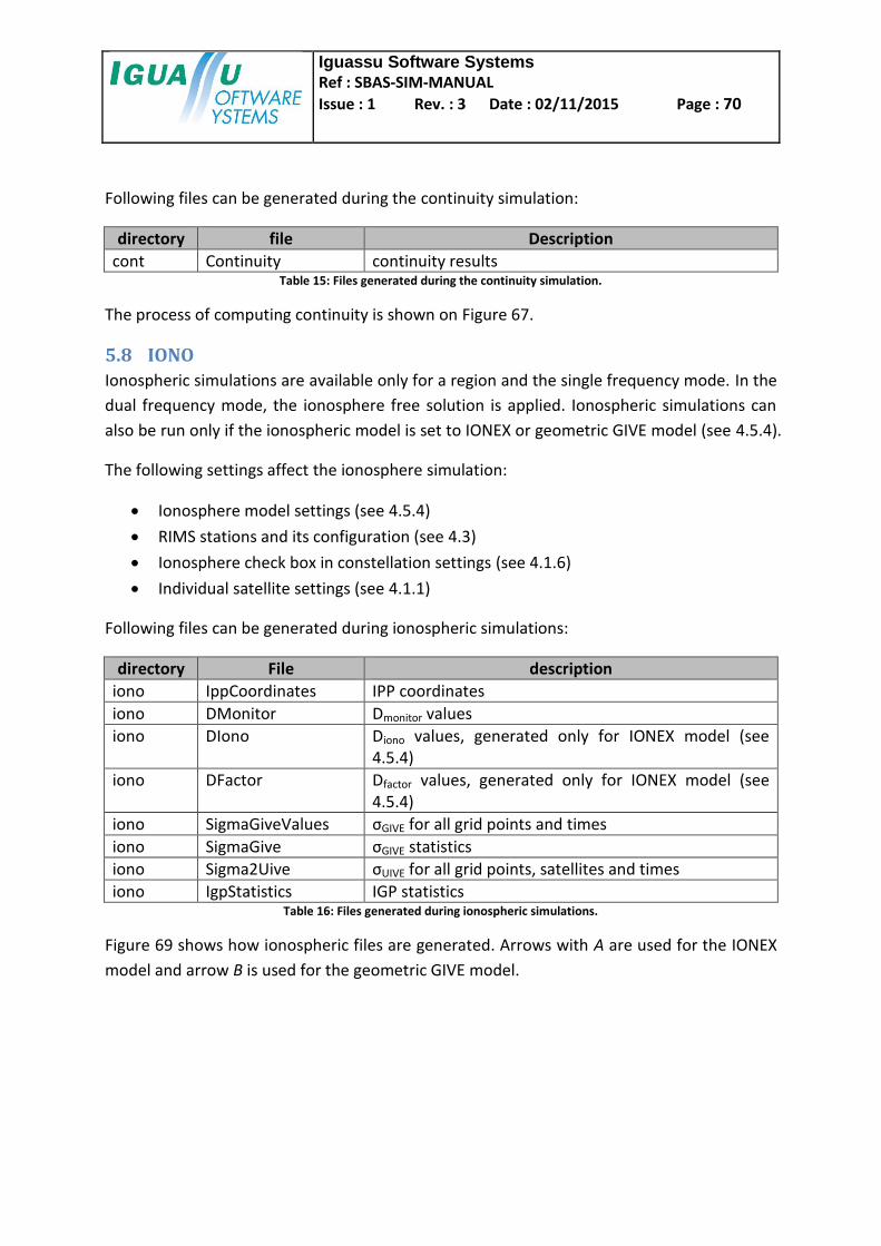
Iguassu Software Systems
Ref : SBAS-SIM-MANUAL
Issue : 1 Rev. : 3 Date : 02/11/2015 Page : 70
Following files can be generated during the continuity simulation:
directory file Description
cont Continuity continuity results Table 15: Files generated during the continuity simulation.
The process of computing continuity is shown on Figure 67.
5.8 IONO
Ionospheric simulations are available only for a region and the single frequency mode. In the
dual frequency mode, the ionosphere free solution is applied. Ionospheric simulations can
also be run only if the ionospheric model is set to IONEX or geometric GIVE model (see 4.5.4).
The following settings affect the ionosphere simulation:
Ionosphere model settings (see 4.5.4)
RIMS stations and its configuration (see 4.3)
Ionosphere check box in constellation settings (see 4.1.6)
Individual satellite settings (see 4.1.1)
Following files can be generated during ionospheric simulations:
directory File description
iono IppCoordinates IPP coordinates
iono DMonitor Dmonitor values
iono DIono Diono values, generated only for IONEX model (see 4.5.4)
iono DFactor Dfactor values, generated only for IONEX model (see 4.5.4)
iono SigmaGiveValues σGIVE for all grid points and times
iono SigmaGive σGIVE statistics
iono Sigma2Uive σUIVE for all grid points, satellites and times
iono IgpStatistics IGP statistics Table 16: Files generated during ionospheric simulations.
Figure 69 shows how ionospheric files are generated. Arrows with A are used for the IONEX
model and arrow B is used for the geometric GIVE model.

Iguassu Software Systems
Ref : SBAS-SIM-MANUAL
Issue : 1 Rev. : 3 Date : 02/11/2015 Page : 71
Figure 69: Hierarchy of ionospheric files.
5.8.1 IPP location
Ionospheric pierce point locations are the intersections between RIMS station and satellite
at the ionosphere height. IPPs take into the account ionospheric scintillations as defined in
4.5.4. User can select IPPs for all system, for specific satellites or RIMS.
Figure 70: IPPs around the RIMS in Berlin.
5.8.2 IGP statistics
IGP statistics monitor the situation at every IGP point. The more IPPs are around a particular IGP, the more accurate ionospheric correction this IGP will have. User can limit the maximal

Iguassu Software Systems
Ref : SBAS-SIM-MANUAL
Issue : 1 Rev. : 3 Date : 02/11/2015 Page : 72
distance between IPG and IPP through IGP radius in Dmonitor settings (Figure 46 and Figure 47). IGP statistics computes number of IPPs within the specified distance from every IGP. The graph (Figure 71) shows average values over the whole simulation time. Values are in the positions of IGPs. Total number of IGPs depends on using bands 9 and 10.
Figure 71: The average number of IPPs around an IGP.
5.8.3 Sigma GIVE calculation
Algorithms for computing the σGIVE depend on the ionospheric model:
IONEX ionospheric model: σGIVE is calculated using the equation (10)
Geometric GIVE model: σGIVE depends on number of IPPs around an IGP.
Configuration of the geometric GIVE model is shown on Figure 47.
This analysis provides user with the average and maximum σGIVE values during the simulation
interval. It is also possible to see the σGIVE availability computed from the given limit value.
Figure 72 shows an example of the σGIVE results.

Iguassu Software Systems
Ref : SBAS-SIM-MANUAL
Issue : 1 Rev. : 3 Date : 02/11/2015 Page : 73
Figure 72: σGIVE over ECAC area.
5.9 Monitoring
Satellites can be monitored by RIMS, when the parent constellation is used for ranging (see
4.1.6). A satellite is monitored, when it sees specific RIMS types as explained in 4.1.1.3. This
analysis provides user with a graphical view showing monitored satellites during the
simulation time (Figure 73). The SatMonitor file is generated as shown on Figure 58.

Iguassu Software Systems
Ref : SBAS-SIM-MANUAL
Issue : 1 Rev. : 3 Date : 02/11/2015 Page : 74
Figure 73: Satellites that are monitored during the 24h simulation.
5.10 DOC simulations
DOC simulation includes XDOC, IDOC and ADOC. Before starting the DOC simulation, it must
be known how many RIMS are seen from a specific satellite.
RIMS has several types: A, B, C, D, E and F. Each of the type can be active/inactive or can be
lost due to specific configuration (mask, random loss, time interval loss, etc.). Satellite is
monitored when see specific number of RIMS types as explained in 4.1.1.3.
In the XDOC, IDOC and ADOC simulation it is important to know how many RIMS are seen
from particular satellite. A RIMS is considered to be seen from a satellite, when it contributes
to the monitoring state. For example, at specific time the following RIMS with active types
are defined:
RIMS Active types
RIMS1 A,B
RIMS2 A,B
RIMS3 A,B
RIMS4 A,B
RIMS5 A,C

Iguassu Software Systems
Ref : SBAS-SIM-MANUAL
Issue : 1 Rev. : 3 Date : 02/11/2015 Page : 75
RIMS6 A,D
RIMS7 A,E
RIMS8 C,D,E,F
RIMS9 D,E,F Table 17: Example of RIMS and its active types.
The Satellite1 is in contact with all 9 RIMS and its types. The Satellite1 is considered
monitored, when it sees at least 5 RIMS A, and 3 RIMS B. Satellite1 is monitored, because it
sees 7 RIMS A and 4 RIMS B. But only the first 7 RIMS contribute to the monitoring state
(RIMS8 and RIMS9 have no effect on monitoring). Therefore for the XDOC, IDOC and ADOC
simulation the Satellite1 sees 7 RIMS.
Monitoring conditions on RIMS prevail and they can be turned off through a checkbox in the
DOC simulation settings window.
Following files can be generated during DOC simulations:
directory file description
doc Xdoc XDOC results
doc Idoc IDOC results
doc Adoc ADOC results Table 18: Files generated during DOC simulations.
Figure 74 shows the computational order of DOC files.
Figure 74: Hierarchy of DOC files.
5.10.1 XDOC
XDOC Simulation shows the minimum number of RIMS for particular number of satellites (or
for all satellites). Before the simulation starts, the user specifies the number of satellites
(nsat).
The computation of XDOC first lists monitored satellites for a particular grid point at specific
time. Each satellite sees some RIMS. The lowest number of monitored RIMS for nsat is taken.
In the case where all satellites are used, the lowest number for all satellites is taken.

Iguassu Software Systems
Ref : SBAS-SIM-MANUAL
Issue : 1 Rev. : 3 Date : 02/11/2015 Page : 76
Figure 75: XDOC simulation - minimal number of RIMS for 6 satellites.
5.10.2 IDOC
IDOC Simulation shows the number of satellites monitored at least by a specific number of
RIMS. Before the simulation starts, the user specifies the number of RIMS (nRIMS).
The computation of IDOC first lists monitored satellites for a particular grid point at specific
time. Each satellite sees some RIMS. IDOC computes the number of satellites that are able to
see at least nRIMS RIMS. The simulation shows the minimal value during the simulation
interval.
5.10.3 ADOC
ADOC Simulation shows the availability and coverage time when specific number of satellites
is monitored by specific number of RIMS. Before the simulation starts, the user sets the
number of satellites (nsat) and the number of RIMS (nRIMS).
The computation of ADOC first lists monitored satellites for a particular grid point at specific
time. Each satellite sees some RIMS. The lowest number of monitored RIMS for nsat is taken.
If this lowest number is equal or higher than nRIMS, the grid point is declared as available for
ADOC at that given time. Apart from the availability, the ADOC simulation also shows the
coverage time.
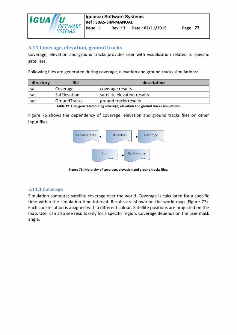
Iguassu Software Systems
Ref : SBAS-SIM-MANUAL
Issue : 1 Rev. : 3 Date : 02/11/2015 Page : 77
5.11 Coverage, elevation, ground tracks
Coverage, elevation and ground tracks provides user with visualization related to specific
satellites.
Following files are generated during coverage, elevation and ground tracks simulations:
directory file description
sat Coverage coverage results
sat SatElevation satellite elevation results
sat GroundTracks ground tracks results Table 19: Files generated during coverage, elevation and ground tracks simulations.
Figure 76 shows the dependency of coverage, elevation and ground tracks files on other
input files.
Figure 76: Hierarchy of coverage, elevation and ground tracks files.
5.11.1 Coverage
Simulation computes satellite coverage over the world. Coverage is calculated for a specific time within the simulation time interval. Results are shown on the world map (Figure 77). Each constellation is assigned with a different colour. Satellite positions are projected on the map. User can also see results only for a specific region. Coverage depends on the user mask angle.

Iguassu Software Systems
Ref : SBAS-SIM-MANUAL
Issue : 1 Rev. : 3 Date : 02/11/2015 Page : 78
Figure 77: Coverage simulation.
5.11.2 Elevation
Elevation is similar to the coverage simulation. The Simulate elevation button is just below
the Simulate Coverage button. User first specifies the satellite and the time, for which
elevation will be simulated.

Iguassu Software Systems
Ref : SBAS-SIM-MANUAL
Issue : 1 Rev. : 3 Date : 02/11/2015 Page : 79
Figure 78: Elevation simulation.
5.11.3 Ground tracks
Ground track is the path on the Earth's surface directly below the satellite. It is the projection of its orbit onto the Earth. Simulation is performed over the world (Figure 79). Constellations have different colours. Satellite ground tracks can be manually selected and deselected. User can also zoom graph to a region.

Iguassu Software Systems
Ref : SBAS-SIM-MANUAL
Issue : 1 Rev. : 3 Date : 02/11/2015 Page : 80
Figure 79: Ground tracks simulation showing one GPS and on Galileo satellite.
5.12 Delta map
Delta map is the difference between 2 simulations. Both simulations must be of the same type. Sources are simulation files generated before. Each simulation type supported by delta map has its own data file:
DOP region statistics (file DeltaDopStatistics.dat)
DOP region availability (file DeltaDopAvailability.dat)
NSE region statistics (file DeltaNseStatistics.dat)
NSE region availability (file DeltaNseAvailability.dat)
XPL region statistics (file DeltaXplStatistics.dat)
Region availability (file DeltaAvailability.dat)
Continuity (file DeltaContinuity.dat)
IGP statistics (file DeltaIgpStat.dat)
Sigma GIVE (file DeltaGive.dat)
XDOC (file DeltaXdoc.dat)
IDOC (file DeltaIdoc.dat)
ADOC (file DeltaAdoc.dat). Simulation files are stored in the scenario folder. Before doing delta map user should have 2 different simulation files of the same type (from 2 different scenarios). Both files must store results for the same region.

Iguassu Software Systems
Ref : SBAS-SIM-MANUAL
Issue : 1 Rev. : 3 Date : 02/11/2015 Page : 81
5.13 3D view
View situation tool has 2 functions: 3D View and Sky plot. 3D view shows three-dimensional Earth with satellites on their orbits. More it can provide user with simulation dynamic plots (Figure 80).
Figure 80: 3D view showing dynamic HPL and information for the selected satellite.
The view is rotated by holding the left mouse button and moving the mouse. Right button is used to move in space and mouse wheel is used for zooming. Context menu can be used if a mouse does not have a wheel. There is also the option to return to the default view. Clicking on the satellite displays its orbit. Actual data are shown in the right panel. Orbits and names of all satellites can also be seen by selecting appropriate check boxes. When dynamic graphs are used, right panel contains coloured simulation scale. At the bottom is the time control. User can scroll to a specific time or use buttons on the left to start the animation. Simulation speed says how faster the simulation goes with respect to the real time. When showing dynamic graphs, animation will be slower. On the right the time in GPS and UTC format is displayed. Camera can be set to inertial or to ECEF mode. Inertial camera shows the situation as seen from the inertial system, where satellite orbits are fixed in space. Earth is rotating during the

Iguassu Software Systems
Ref : SBAS-SIM-MANUAL
Issue : 1 Rev. : 3 Date : 02/11/2015 Page : 82
animation. ECEF camera is used to see always the same part of the Earth. In this mode satellite orbits will be rotating.
5.14 Sky plot
Sky plot is the second function of the view situation tool. For a point simulation, it is possible see positions of satellites on the sky during the whole simulation time (Figure 81).
Figure 81: Sky plot showing visibility of satellites from Paris.
Check boxes in the left panel are used to show or hide satellite names or trajectories. The red circle marks the user mask angle. At the bottom is the animation panel with the same functions as in 3D view. Sky plot can also show actual positions of existing GPS satellites. First the coordinates must be set to user location. Then current GPS almanac shall be loaded (simulation start time is automatically changed to the current time). After running the simulation, actual satellite positions can be seen from the user area.
6 Graphs There are many different types of graphs that can be viewed in the SBAS Simulator. Some of
the graph types are described in other sections of this manual: Both types of Point graph are
described in 5.3.1 and 5.3.2, Coverage graph is described in 5.11.1, Ground tracks graph is

Iguassu Software Systems
Ref : SBAS-SIM-MANUAL
Issue : 1 Rev. : 3 Date : 02/11/2015 Page : 83
described in 5.11.3, 3D view is described in 5.13, Sky plot is described in 5.14 and the
Monitoring graph is described in 5.9.
6.1 Region graph
The Region graph shows a specified region of the world map (or the whole world map) with
desired data overlapping the world map’s region. An example of a Region graph can be seen
in Figure 63. The graph’s window has many controls that modify the way the graph is
displayed on the screen.
It is also possible to export the graph into a file: The Export graph button in the lower right
corner serves for this purpose. Before the graph is saved to a file, the pixel resolution of the
image has to be chosen. User shall also specify the path to the file and the file format (bmp,
jpg, wbmp, png and gif).
6.1.1 Region graph controls
Apart from buttons on the right side of the window, which are used to zoom in, zoom out
and also move the graph when the view is zoomed in, there are several controls on the left
side of the window (see Figure 82).
Figure 82: Example of controls on the left side of the Region graph window.

Iguassu Software Systems
Ref : SBAS-SIM-MANUAL
Issue : 1 Rev. : 3 Date : 02/11/2015 Page : 84
Show Z values checkbox is used to enable and disable the printing of z values inside the
graph area. Show RIMS checkbox is used to enable or disable the printing of RIMS in the
graph area.
The Levels button is used to modify the number of levels and also the maximum and
minimum of the range of these levels. For example: In Figure 82 the number of levels is set
to 10 (represented by 10 different colours in the bar above the Levels button), minimum is
set to 0.69 and maximum to 1.04 (both of these values are also seen in the bar above the
Levels button).
The Reverse colours button reverses the order of colours shown in the bar (see Figure 82).
For example: In Figure 82 the colours go from blue to red as the values grow, reversing the
colours would cause the colours to go from red to blue as the values grow.
The Service area layers dropdown menu is used to select which region is to be highlighted in
the graph area. Apart from regions specified in section 4.2.1, the satellite map can also be
shown.
If Draw break line is selected, a black line is drawn in the graph area, separating lower and
higher values by the specified break value. Alternative way to display such division into two
disjoint subsets is to select Use only 2 colours: Instead of a black line the graph is coloured
only using two colours, red (or blue if the Use blue as max is checked) areas contain values
greater than the break and white areas contain values less than the break.
7 SBAS Simulator Files
7.1 Simulation steps
Each simulation can be divided into simulation steps which are subtasks of the main process. They are simple simulations with defined input and output. For example to perform DOP simulation the simulator goes through the following steps (see also Figure 58 and Figure 60):
1. Compute satellite positions for all used satellites within the simulation interval (SatPosition file).
2. Use satellite positions and calculate ENU coordinates for user location (Enu file). 3. Use computed ENU coordinates and calculate DOP (DopValues file).
The advantage of separating simulations into steps is the reusability of already computed tasks. Simulation results are saved to simulation files. The last simulation file contains data which are plotted in the graph. Files are saved to the scenario directory. Writing and reading permissions are needed for the scenario directory otherwise it is not possible to run the tool.
7.2 Data and meta-files
Simulation file is actually a set of two files. Both have the same names, but different extensions. Results are stored in data file (*.dat). It is a CSV file with a defined number of

Iguassu Software Systems
Ref : SBAS-SIM-MANUAL
Issue : 1 Rev. : 3 Date : 02/11/2015 Page : 85
columns which are separated by semicolons. Meta file (*.meta) contains various simulator settings that were used when generating data file. Data are stored in the form of parameter-value or CSV lines. First three rows of meta file are:
FILE ID - hash code computed from simulation step input
CRC - cyclic redundancy check of associated data file
COLUMNS – columns in data file.
Input is unambiguously defined for each simulation step. For the same input, each set of files is generated only once. This feature speeds up the simulation process, because some computations can be omitted. COLUMNS specify names of columns in data file. For example TI is the time index looping all simulation times, SI is the satellite index looping all used satellites, RI is the RIMS index of used RIMS. The meaning of other columns should be clear. Before each simulation step following check is done:
1. If data or meta file do not exist, perform the simulation and generate files, otherwise go to 2.
2. If FILE ID is not the same as the input hash code, perform the simulation and generate files, otherwise go to 3.
3. If CRC specified in meta file is not the same as CRC computed from data file, perform the simulation and generate files, otherwise skip this simulation step.
Simulation files are stored in directories under the scenario directory. Directories group similar simulation files. The list of simulation files can be found in tables in section 5.

Iguassu Software Systems
Ref : SBAS-SIM-MANUAL
Issue : 1 Rev. : 3 Date : 02/11/2015 Page : 86
< End of Document >