TMD DISCUSSION PAPER NO. 58

Updating and Estimating a Social Accounting

Matrix Using Cross Entropy Methods

Sherman Robinson Andrea Cattaneo

And Moataz El-Said

International Food Policy Research Institute

Trade and Macroeconomics Division International Food Policy Research Institute

2033 K Street, N.W. Washington, D.C. 20006, U.S.A.

August 2000

TMD Discussion Papers contain preliminary material and research results, and are circulated prior to a full peer review in order to stimulate discussion and critical comment. It is expected that most Discussion Papers will eventually be published in some other form, and that their content may also be revised. This paper is available at http://www.cgiar.org/ifpri/divs/tmd/dp.htm

Updating and Estimating a Social Accounting Matrix Using

Cross Entropy Methods*

by

Sherman Robinson

Andrea Cattaneo

and

Moataz El-Said1

International Food Policy Research Institute

Washington, D.C., U.S.A.

August 2000

Published in: Economic Systems Research, Vol. 13, No.1, pp. 47-64, 2001.

*The first version of this paper was presented at the MERRISA (Macro-Economic Reforms and Regional Integration in Southern Africa) project workshop. September 8 -12, 1997, Harare, Zimbabwe. A version was also presented at the Twelfth International Conference on Input-Output Techniques, New York, 18-22 May 1998. Our thanks to Channing Arndt, George Judge, Amos Golan, Hans Löfgren, Rebecca Harris, and workshop and conference participants for helpful comments. We have also benefited from comments at seminars at Sheffield University, IPEA Brazil, Purdue University, and IFPRI. Finally, we have also greatly benefited from comments by two anonymous referees.

1Sherman Robinson, IFPRI, 2033 K street, N.W. Washington, DC 20006, USA. Andrea Cattaneo, IFPRI, 2033 K street, N.W. Washington, DC 20006, USA. Moataz El-Said, IFPRI, 2033 K street, N.W. Washington, DC 20006, USA.

Abstract

The problem in estimating a social accounting matrix (SAM) for a recent year is to find an

efficient and cost-effective way to incorporate and reconcile information from a variety of

sources, including data from prior years. Based on information theory, the paper presents a

flexible “cross entropy” (CE) approach to estimating a consistent SAM starting from inconsistent

data estimated with error, a common experience in many countries. The method represents an

efficient information processing rule—using only and all information available. It allows

incorporating errors in variables, inequality constraints, and prior knowledge about any part of

the SAM. An example is presented applying the CE approach to data from Mozambique, using a

Monte Carlo approach to compare the CE approach to the standard RAS method and to evaluate

the gains in precision from utilizing additional information.

KEYWORDS: Entropy, cross entropy, social accounting matrices, SAM, input- output, RAS,

Monte Carlo simulations

Table of Contents

1. Introduction ............................................................................................................................... 1

2. Structure of a Social Accounting Matrix (SAM) ....................................................................... 2

3. The RAS Approach to SAM Updating ...................................................................................... 3

4. A Cross Entropy Approach to SAM estimation......................................................................... 4

4.1. Deterministic Approach: Information Theory..................................................................... 5 4.2. Types of Information .......................................................................................................... 7 4.3. Stochastic Approach: Measurement Error .......................................................................... 9

5. Updating a SAM: RAS and Cross-Entropy ............................................................................. 13

6. From Updating to Estimating Using the Cross-Entropy Approach.......................................... 15

7. Conclusion............................................................................................................................... 18

1

1. Introduction

There is a continuing need to use recent and consistent multisectoral economic data to

support policy analysis and the development of economywide models. A Social Accounting

Matrix (SAM) provides the underlying data framework for this type of model and analysis. A

SAM includes both input-output and national income and product accounts in a consistent

framework. Estimating a SAM for a recent year is a difficult and challenging problem. Input-

output data are usually prepared only every five years or so, while national income and product

data are produced annually, but with a lag. To produce a more disaggregated SAM for detailed

policy analysis, these data are often supplemented by other information from a variety of

sources; e.g., censuses of manufacturing, labor surveys, agricultural data, government accounts,

international trade accounts, and household surveys. The problem in estimating a disaggregated

SAM for a recent year is to find an efficient (and cost-effective) way to incorporate and reconcile

information from a variety of sources, including data from prior years.

A standard approach is to start with a consistent SAM for a particular prior period and

“update” it for a later period, given new information on row and column totals, but no

information on the flows within the SAM. The traditional RAS approach, discussed below,

addresses this case. However, in practice, one often starts from an inconsistent SAM, with

incomplete knowledge about both row and column sums and flows within the SAM.

Inconsistencies can arise from measurement errors, incompatible data sources, or lack of data.

What is needed is an approach to estimating a consistent set of accounts that not only uses the

existing information efficiently, but also is flexible enough to incorporate information about

various parts of the SAM.

In this paper, we propose a flexible “cross entropy” (CE) approach to estimating a

consistent SAM starting from inconsistent data estimated with error. The method is very flexible,

incorporating errors in variables, inequality constraints, and prior knowledge about any part of

the SAM (not just row and column sums). The next section presents the structure of a SAM and

a mathematical description of the estimation problem. The following section describes the RAS

2

procedure, followed by a discussion of the cross entropy approach. Next we present an

application to Mozambique demonstrating gains from using increasing amounts of information.2

2. Structure of a Social Accounting Matrix (SAM)

A SAM is a square matrix whose corresponding columns and rows present the

expenditure and receipt accounts of economic actors. Each cell represents a payment from a

column account to a row account. Define T as the matrix of SAM transactions, where ,i jt is a

payment from column account j to row account i. Following the conventions of double-entry

bookkeeping, total receipts (income) and expenditure of each actor must balance. That is, for a

SAM, every row sum must equal the corresponding column sum:

, ,i i j j ij j

y t t= =∑ ∑ (1)

Where yi is total receipts and expenditures of account i.

A SAM coefficient matrix, A, is constructed from T by dividing the cells in each column

of T by the column sums:

,,

i ji j

j

ta

y= (2)

By definition, all the column sums of A must equal one, so the matrix is singular. Since column

sums must equal row sums, it also follows that (in matrix notation):

=y Ay (3)

A typical national SAM includes accounts for production (activities), commodities,

factors of production, and various actors (“institutions”), which receive income and demand

goods. The structure of a simple SAM is given in Table 1. Activities pay for intermediate inputs,

factors of production, and indirect taxes, and receive payments for sales of their output. The

commodity account buys goods from activities (producers) and the rest of the world (imports),

2An appendix with the computer code in the GAMS language used in the procedure is available upon request. The method has been used to estimate SAM’s for a number of African countries (Botswana, Malawi, Mozambique, Tanzania, Zambia, and Zimbabwe) and a few other countries (e.g., Brazil, Mexico, North Korea, and the United States). The Mozambique application is described below.

3

and pays tariffs on imported goods, while it sells commodities to activities (intermediate inputs)

and final demanders (households, government, investment, and the rest of the world). In this

SAM, gross domestic product (GDP) at factor cost equals payments by activities to factors of

production, or value added. GDP at market prices equals GDP at factor cost plus indirect taxes

and tariffs, which also equals total final demand (consumption, investment, and government)

plus exports minus imports.

<< Table 1 >>

The matrix of column coefficients, A, from such a SAM provides raw material for much

economic analysis and modeling. For example, the intermediate-input coefficients (computed

from the “use” matrix) are Leontief input-output coefficients. The coefficients for primary

factors are “value added” coefficients and give the distribution of factor income. Column

coefficients for the commodity accounts represent domestic and import shares, while those for

the various final demanders provide expenditure shares. There is a long tradition of work which

starts from the assumption that these various coefficients are fixed, and then develops various

linear multiplier models. The data also provide the starting point for estimating parameters of

nonlinear, neoclassical production functions, factor-demand functions, and household

expenditure functions.

In principle, it is possible to have negative transactions, and hence coefficients, in a

SAM. Such negative entries, however, can cause problems in some of the estimation techniques

described below and also may cause problems of interpretation in the coefficients. A simple

approach to dealing with this issue is to treat a negative expenditure as a positive receipt or a

negative receipt as a positive expenditure. That is, if ,i jt is negative, we simply set the entry to

zero and add the value to ,j it . This “flipping” procedure will change row and column sums, but

they will still be equal.

3. The RAS Approach to SAM Updating

The classic problem in SAM estimation is the problem of “updating” an input-output

matrix when we have new information on the row and column sums, but do not have new

4

information on the input-output flows. The generalization to a full SAM, rather than just the

input-output table, is the following problem. Find a new SAM coefficient matrix, *A , that is in

some sense “close” to an existing coefficient matrix, A , but yields a SAM transactions matrix,

*T , with the new row and column sums. That is:

* * *, ,i j i j jt a y= (4)

* * *, ,i j j i i

j j

t t y= =∑ ∑ (5)

Where y* are known new row and column sums.

A classic approach to solving this problem is to generate a new matrix *A from the old

matrix A by means of “biproportional” row and column operations:

*, ,i j i i j ja r a s= (6)

or, in matrix terms:

* ˆˆ=A RAS (7)

where the hat indicates a diagonal matrix of elements ir and js . Bacharach (1970) shows that

this “RAS” method works in that a unique set of positive multipliers (normalized) exists that

satisfies the biproportionality condition and that the elements of R and S can be found by a

simple iterative procedure.3

4. A Cross Entropy Approach to SAM estimation

The estimation problem is that, for an n-by-n SAM, we seek to identify n2 unknown non-

negative parameters (the cells of T or A), but have only 2n–1 independent row and column

adding-up restrictions. The RAS procedure imposes the biproportionality condition, so the

3For the method to work, the matrix must be “connected,” which is a generalization of the notion of “indecomposable” (Bacharach, 1970, p. 47). For example, this method fails when a column or row of zeros exists because it cannot be proportionately adjusted to sum to a non-zero number. Note also that the matrix need not be square. The method can be applied to any matrix with known row and column sums: for example, an input-output matrix that includes final demand columns (and is hence rectangular). In this case, the column coefficients for the final demand accounts represent expenditure shares and the new data are final demand aggregates.

5

problem reduces to finding 2n–1 ir and js coefficients (one being set by normalization), yielding

a unique solution. The general problem is that of estimating a set of parameters with little

information. If all we know are row and column sums, there is not enough information to

identify the coefficients, let alone provide degrees of freedom for estimation. Updating, in this

framework, becomes a special case of the more general estimation problem for which the

information provided is the balanced SAM to be updated and new row and column totals.

In a recent book, Golan, Judge, and Miller (1996) suggest a variety of estimation

techniques using “maximum entropy econometrics” to handle such “ill-conditioned” estimation

problems. Golan, Judge, and Robinson (1994) apply this approach to estimating a new input-

output table given knowledge about row and column sums of the transactions matrix—the classic

RAS problem discussed above. We extend this methodology to situations where there are

different kinds of prior information than knowledge of row and column sums.

4.1. Deterministic Approach: Information Theory

The estimation philosophy adopted in this paper is to use all, and only, the information

available for the estimation problem at hand. The first step we take in this section is to define

what is meant by “information”. We then describe the kinds of information that can be

incorporated and how to do it. This section focuses on information concerning non-stochastic

variables while the next section will introduce the use of information on stochastic variables.

The starting point for the cross entropy approach is information theory as developed by

Shannon (1948). Theil (1967) brought this approach to economics. Consider a set of n events E1,

E2, …, En with probabilities q1, q2,…, qn (prior probabilities). A message comes in which

implies that the odds have changed, transforming the prior probabilities into prior probabilities

p1, p2,…, pn. Suppose for a moment that the message confines itself to one event Ei. Following

Shannon, the “information” received with the message is equal to -ln pi. However, each Ei has its

own prior probability qi, and the “additional” information from pi is given by:

[ ]ln ln lnii i

i

pp q

q− = − − (8)

Taking the expectation of the separate information values, we find that the expected information

value of a message (or of data in a more general context) is

6

( )1

: lnn

ii

i i

pI p q p

q=

− = −∑ (9)

where I(p:q) is the Kullback-Leibler (1951) measure of the “cross entropy” (CE) distance

between two probability distributions.4 Kapur and Kenavasan (1992, Chapter 4) describe various

axiomatic approaches that uniquely define the entropy measure as an appropriate measure of

information and that justify the use of the CE measure for inference. For estimation, the

approach is to find a set of p’s that minimize the cross entropy between the probabilities and the

prior q’s, and that are consistent with the information in the data.5

Golan, Judge, and Robinson (1994) use a cross entropy formulation to estimate the

coefficients in an input-output table. They set up the problem as finding a new set of A

coefficients which minimizes the entropy distance between the prior A and the new estimated

coefficient matrix.6

,,

,

min ln i ji j

i j i j

aa

a

∑∑ (10)

Subject to:

* *,i j j i

j

a y y=∑ (11)

, ,1 and 0 1j i j ij

a a= ≤ ≤∑ (12)

The solution is obtained by setting up the Lagrangian for the above problem and solving it.7 The

outcome combines the information from the data and the prior:

4Note that the cross-entropy “distance” is not a norm. It is neither symmetric nor satisfies the triangle inequality. 5If the prior distribution is uniform, representing total ignorance, the method is equivalent to the “Maximum Entropy” estimation criterion (see Kapur and Kesavan, 1992; pp. 151-161).

6The intuition underlying this minimization problem is that it aims to minimize the expected information value of additional data given what we know (sample and prior).

7The problem has to be solved numerically because no closed form solution exists.

7

( )

( )*

,

, *,

,

exp

exp

i j i j

i j

i j i ji j

a ya

a y

λ

λ=

∑ (13)

where iλ are the Lagrange multipliers associated with the information on row and column sums,

and the denominator is a normalization factor.

The expression is analogous to Bayes’ Theorem, whereby the posterior distribution

,( )i ja is equal to the product of the prior distribution ,( )i ja and the likelihood function

(probability of drawing the data given parameters we are estimating), dividing by a

normalization factor to convert relative probabilities into absolute ones. The analogy to Bayesian

estimation is that the approach can be seen as an efficient Information Processing Rule (IPR)

whereby we use additional information to revise an initial set of estimates (Zellner, 1988, 1990).

In this approach an “efficient” estimator satisfies what Zellner (1988) describes as the

“Information Conservation Principle”: the estimation procedure should neither ignore any of the

input information nor inject any false information. It can also be shown that the CE estimators

are consistent and, given assumptions about the form of the underlying distribution, have

maximum likelihood properties (Golan, Judge, and Miller, 1996).

4.2. Types of Information

Information for SAM estimation comes in many forms:

1. Priors. A SAM from an earlier year provides information about the new coefficients. The

approach is to estimate a new set of coefficients “close” to the prior, using new

information to “update” the prior.

2. Moment constraints. The most common kind of information to have is data on some or all

of the row and column sums of the new SAM. Treating the column coefficients as

analogous to probabilities, assuming known column sums in equation (11) is equivalent

to knowing averages of the column sums, weighting by the coefficients—or first

moments of the distributions. While the RAS procedure is based on knowing all row and

column sums, it is only one of several possible sources of information in CE estimation.

8

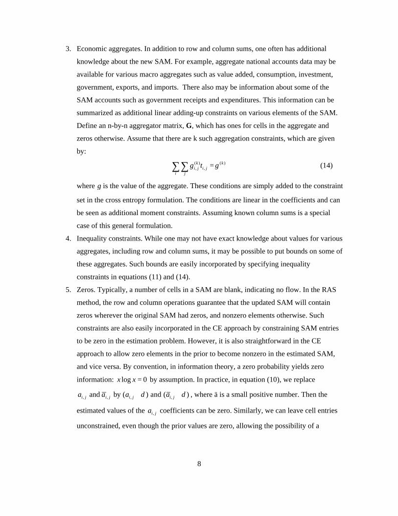
3. Economic aggregates. In addition to row and column sums, one often has additional

knowledge about the new SAM. For example, aggregate national accounts data may be

available for various macro aggregates such as value added, consumption, investment,

government, exports, and imports. There also may be information about some of the

SAM accounts such as government receipts and expenditures. This information can be

summarized as additional linear adding-up constraints on various elements of the SAM.

Define an n-by-n aggregator matrix, G, which has ones for cells in the aggregate and

zeros otherwise. Assume that there are k such aggregation constraints, which are given

by:

( ) ( ), ,k k

i j i ji j

g t γ=∑∑ (14)

where γ is the value of the aggregate. These conditions are simply added to the constraint

set in the cross entropy formulation. The conditions are linear in the coefficients and can

be seen as additional moment constraints. Assuming known column sums is a special

case of this general formulation.

4. Inequality constraints. While one may not have exact knowledge about values for various

aggregates, including row and column sums, it may be possible to put bounds on some of

these aggregates. Such bounds are easily incorporated by specifying inequality

constraints in equations (11) and (14).

5. Zeros. Typically, a number of cells in a SAM are blank, indicating no flow. In the RAS

method, the row and column operations guarantee that the updated SAM will contain

zeros wherever the original SAM had zeros, and nonzero elements otherwise. Such

constraints are also easily incorporated in the CE approach by constraining SAM entries

to be zero in the estimation problem. However, it is also straightforward in the CE

approach to allow zero elements in the prior to become nonzero in the estimated SAM,

and vice versa. By convention, in information theory, a zero probability yields zero

information: log 0x x = by assumption. In practice, in equation (10), we replace

, , , , and by ( ) and ( )i j i j i j i ja a a aδ δ+ + , where ä is a small positive number. Then the

estimated values of the ,i ja coefficients can be zero. Similarly, we can leave cell entries

unconstrained, even though the prior values are zero, allowing the possibility of a

9

nonzero entry appearing (say, drawing on information about possible technological

changes in which the input-output coefficient matrix becomes more dense).

4.3. Stochastic Approach: Measurement Error

Most applications of economic models to real world issues must deal with the problem of

extracting results from data or economic relationships with noise. In this section we generalize

our approach to cases where: (i) row and column sums are not fixed parameters but involve

errors in measurement; and (ii) the initial estimate, A , is not based on a balanced SAM.

Consider the standard regression model:

y = x â + e (15)

where â is the coefficient vector to be estimated, y represents the vector of dependent variables,

x the independent variables, and e is the error term. Consider the standard assumptions made in

regression analysis from the perspective of information theory.

• There is plenty of data providing adequate degrees of freedom for estimation.

• The error e is usually assumed to be normally distributed with zero mean and constant

variance. This represents a lot of information on the error structure. The only parameter

that needs to be estimated is the error variance. Given these assumptions, we need only use

information in the form of certain moments of the data, which summarize all the

information required to carry out efficient estimation: ( )ˆ ′ ′-1â = x x x y

• On the other hand, no prior information is assumed about the parameters. The null

hypothesis is â = 0, and we assume that no other information is available about â .

• The independent variables are non-stochastic, meaning that it is in principle possible to

repeat the sample with the same independent variables.

These assumptions are extremely constraining when estimating a SAM because little is

known about the error structure and data are scarce. SAM estimation is not a statistical model

where the issue is specifying a random error generating process, but a problem of estimation in

10

the presence of measurement error.8 Finally, data such as parameter values for previous years,

which are often available when estimating a SAM, provide information about the current SAM,

but this information cannot be put to productive use in the standard regression model. Compared

to the standard model, we have little data and know little about the errors, but we have a lot of

information in a variety of forms about the coefficients to be estimated.

There have been a number of efforts to apply statistical methods to SAM estimation. See,

for example Barker et al. (1984), van der Ploeg (1982), and Toh (1998).The approach is to

specify some kind of quadratic loss function and assume information about the statistical

properties of the error distributions. Harrigan and Buchanan (1984) argue persuasively for the

advantages of a constrained maximization estimation approach in terms of flexibility, but are

aware of the statistical problems. Harrigan and McNicoll (1986) state (p. 1065) that “even where

inequality restrictions give way to equalities, the assumptions required to sustain statistical

interpretation are extremely demanding.” Byron (1978) and Schneider and Zenios (1990) also

argue in favor of a constrained maximization approach, and are also skeptical of imposing strong

statistical assumptions.

Harrigan (1990) compares the use of a quadratic positive definite (QPD) objective function

with the Kullback-Leibler cross-entropy (CE) measure. He concludes that both “possess the

desirable property that they give posterior estimates which better reflect the unknown, true

values than do the associated prior estimates.” He then goes on to argue that one cannot prove

the superiority of either the QPD or CE approaches in terms of the relative closeness of their

posterior estimates to the true values, using either measure of closeness.9 From the perspective of

information theory, however, one can show that using any objective function other than the CE

measure implicitly injects additional unwarranted information into the estimation procedure

(Golan, Judge, and Miller, 1996). If the additional information is “correct,” then the resulting

8The problem is analogous to the distinction between errors in equations and errors in variables in standard regression analysis. See, for example, Judge et al. (1985). Golan and Vogel (1997) describe an errors in equations approach to the SAM estimation problem.

9One should note, however, that the distinction between the QPD and CE approaches is not necessarily great. Golan, Judge, and Miller (1996, pp 30-31) show that one can approximate the CE minimand using a weighted squared error measure.

11

estimators might be closer to the true values, but there is no prior reason to make such an

assumption—the CE estimation principle is to use all but only the information available.

We extend the cross entropy criterion to include an “errors in variables” formulation where

the independent variables are assumed to be measured with noise, as opposed to the “errors in

equations” specification, where the process is assumed to include random noise. Rewrite the

SAM equation and the row/column sum consistency constraints as:

[ ]y = A x + e = Ax + Ae (16)

= +y x e (17)

where y is the vector of row sums and x, measured with error e, is the known vector of column

sums, which represents our prior on the column and row sums. In our case, we assume that the

initial column sums in the data are the best prior estimate. One could use alternative estimates

(e.g. initial row sums). Equation 17 reflects the requirement that column and row sums must be

equal. Following Golan, Judge, and Miller (1996, chapter 6), we write the errors as a weighted

average of known constants as follows:

, ,i i w i ww

e w v= ∑ (18)

subject to the weights being between zero and one, and summing to one:

, ,1 and 0 1i w i ww

w w= ≤ ≤∑ (19)

In the estimation, the weights are treated as probabilities to be estimated. The constants, v ,

define the “support set” for the errors (using a bar to indicate that they are not variables) and,

along with a specified prior for the weights, define a prior for the error distribution. The support

set is usually chosen to yield a prior symmetric distribution with moments depending on the

number of elements in the set W. In general, one can add more v’s and W’s to incorporate more

potential information about the error distribution (e.g., more moments, including variance,

skewness, and kurtosis). In our case, we specified a support set with three elements and a

uniform prior for the weights. The support set is specified so that 2 1 30 and v v v= = − , implying a

prior on the error distribution with mean zero and variance 2 2w w

w

w vσ = ∑ . One can specify a

separate prior for every error, if desired, but the main point is that it is only a prior, not a

maintained hypothesis about the error distribution.

12

Given knowledge about the error bounds, equations (17), (18) and (19) are added to the

constraint set and equation (16) replaces the SAM equation (equation 3). The problem is messier

in that the SAM equation is now nonlinear, involving the product of A and e. The minimization

problem is to find a set of A’s and W’s that minimize cross entropy including a term in the errors:

( ) , , , ,

, , ,

ln ln

1ln ln

i j i j i j i ji j i j

i w i w i wi w i w

I a a a a

w w wn

= −

+ −

∑∑ ∑∑

∑∑ ∑∑

A, W : A

(20)

subject to the constraint equations that column and row sums be equal, and that the W’s and A’s

fall between zero and one (where n is the number of elements in the error support set W,

implying a uniform prior), and any other known aggregation inequalities or equalities.

Equation (20) is minimized with respect to the A’s (SAM coefficients) and W’s (weights

on the error term), where the W’s are treated like the A’s. In the estimation procedure, the terms

involving the A’s and W’s are assigned equal weights, reflecting an equal preference for

“precision” (closeness to the prior A’s) in the estimates of the parameters, and “prediction” (the

W’s or the “goodness of fit” of the equation on row and column sums). Golan, Judge, and Miller

(1996) report Monte Carlo experiments where they explore the implications of changing these

weights and conclude that equal weighting of precision and prediction is reasonable.

Another source of measurement error may arise if the initial SAM, A , is not itself a

balanced SAM. That is, its corresponding rows and columns may not be equal. This situation

does not change the cross entropy estimation procedure, but implies that it is not possible to

achieve a cross entropy measure of zero because the prior is not feasible. The idea is to find a

new feasible SAM that is “entropy-close” to the infeasible prior.

Finally, Golan, Judge, and Robinson (1994) discuss a specification where each element in

the SAM is assumed to be measured with error. In this case, each element has a separate error

component with a “weak” prior on its distribution in the sense of specifying only a support set.

The result is that the procedure involves a large number of additional weights to be estimated,

but generates measures of the precision of the estimates cell by cell. The approach is closely

analogous to the approach suggested by Byron (1978) in which he assumes that one starts with

detailed knowledge of the cell-by-cell error distributions, including means and variances. In the

13

CE approach, however, only very weak assumptions need be made about these error

distributions.10

5. Updating a SAM: RAS and Cross-Entropy

To illustrate the use of the proposed cross entropy estimator and to compare its properties

to that of the RAS method, we apply both methods to update a 1994 macro SAM for

Mozambique (Table 2).11 Monte Carlo simulations are carried out by starting from the balanced

SAM and then randomly imposing new row and column totals. The SAM is then updated to be

consistent with the new totals using both the RAS and the cross-entropy methods. Since we

change only row and column totals, we have no idea what the “true” updated SAM should be and

can therefore only compare the results of the two methods in terms of how different they are. We

compare outcomes using two standard distance measures, the root mean squared deviation

(RMSD) of either (1) the new SAM values or (2) its column coefficients, both relative to those of

the original SAM.

As noted in the literature, the RAS and the cross-entropy methods are equivalent if the

CE method uses as an objective a single cross-entropy measure (cell coefficients measured

relative to the sum of all flows in the SAM) instead of using the sum of column cross-entropies

(normalized relative to column totals).12 Intuitively, the RAS method tries to maintain the value

structure (flow-dependent) while the CE method seeks to maintain the coefficient structure

(column-coefficient-dependent).13 Assuming the same information (knowledge of row/column

sums), we would expect the RAS results to be closer to the original SAM values than the CE

10In applying the CE method to SAM coefficients, one must take care when interpreting the resulting statistics because the parameters being estimated are not probabilities, although the column coefficients satisfy the same axioms. While such a procedure is common in the entropy estimation literature, the cell-by-cell approach taken in Golan, Judge, and Robinson (1994) does not rely on any assumptions about the nature of the coefficients. They found the estimated coefficients from the two approaches to be extremely close, and argued that the cell-by-cell approach was useful in yielding information about the reliability of each cell estimate. 11Arndt, et al. (1997) describe the Mozambique SAM in detail. 12See, for example, Bacharach (1970), Schneider and Zenios (1990), and McDougal (1999). 13McDougal (1999) shows that the RAS method is also equivalent to maximizing a weighted sum of the column-coefficient cross-entropies, where the weights are the row (or column) sum values. The RAS method can be seen as treating column and row coefficients symmetrically, and is a special case of the CE method.

14

method relative to the SAM flows. Similarly, the CE results should be closer to the original

coefficient matrix.

If we are seeking to use the updated SAM to estimate column coefficients, which is

commonly the case when the SAM is used to do multiplier analysis or provide various share

coefficients for a CGE model, then it is desirable to express the information contained in the

original SAM in terms of column coefficients, which a priori favors the CE approach. That is,

the new estimates will be closer to the prior for the CE method, given the same additional

information (in the form of new column/row sums). On the other hand, if primary interest is in

the nominal flows, or if row coefficients are as important as column coefficients, then the RAS

approach appears more desirable a priori. As noted above, the RAS method is a special case of

the CE method, using a particular cross-entropy minimand and assuming only knowledge of row

and column sums. So it is feasible to use the CE approach as a generalization of the RAS method

when different types of information are available. An important question is whether the two

approaches differ significantly in practice. If not, then it may not matter much which is used in

most cases.

The procedure adopted for the Monte Carlo simulations is as follows: three row totals

were randomly perturbed relative to the balanced Macro SAM, and the perturbed values were

imposed as the new row and column totals in the updating process. The perturbed values were

generated by sampling from a set of normal distributions with increasing standard deviations: the

values starting from 1% and increasing up to 10% in 1% increments every 100 samples, making

for a total of one thousand runs. Figure 1a is a scatter plot of the root mean square deviation

(RMSD) of the SAM flows after updating relative to the initial flows. On the Y-axis is the

RMSD obtained using the entropy method, while on the X-axis is the RMSD according to the

RAS. The solid line at 45 degrees represents situations where the two methods give the same

answer. The dotted line is a linear regression fitting the sample.

Figure 1a indicates that the RAS and CE methods perform similarly in flow terms. The

points are grouped around the 45-degre line, with no strong differences in the degree to which

the flow estimates deviate from the prior under the two approaches. The regression line is

slightly above the 45-degree line, indicating that, as expected, the RAS method yields results

closer to the prior flows, but the differences are not great.

15

<<Figure 1>>

The results are very different when the two methods are compared in terms of deviation of the

column coefficients after updating relative to the initial coefficients. Figure 1b unequivocally

shows that, in terms of column coefficients, updating by the cross entropy method yields

estimates much closer to the prior coefficients than updating with the RAS method. The dotted

regression line indicates that the coefficient RMSD is about 25% lower using the cross entropy

method than with the RAS.14

The conclusion to be drawn from the comparison of the RAS and the cross entropy

method is that if the analyst is concerned column coefficients, then the cross entropy method

appears superior to the RAS method. If, on the other hand, the focus is on the flows in the SAM,

then the two methods are very close, with the RAS method performing slightly better.

6. From Updating to Estimating Using the Cross-Entropy Approach

In the previous section the comparison between cross entropy and RAS methods was

made in the context of the standard updating problem found in the input-output literature. We

now shift the focus to an application that illustrates a more general formulation of the updating

problem: estimating a SAM given various data sources of varying quality. This is a process that

is often done manually by applied researchers. We show, however, that the CE approach

efficiently uses all the available information for SAM estimation. In fact, many of the manual

operations (or data “adjustments”) can be incorporated into the CE approach. Most importantly,

the estimation problem is set in the context of information theory and the procedure generates

measures of the “importance” of different data used in the estimation process.

The performance of the cross entropy method in this estimation process was tested, once

again, by running Monte Carlo simulations. For one thousand simulations, at each run eight cells

of the originally balanced SAM were chosen at random and perturbed. Each time, the unbalanced

SAM obtained through this procedure was balanced using the cross entropy method. This

procedure was performed assuming varying types of information were available: (i) in the first

14It is interesting to observe that the pattern in the scatter plot of Figure 1b appears to be distributed along two different lines. This dual behavior is probably associated with different moment constraints becoming binding in the entropy method.

16

set of simulations no information was assumed other than correspondong row and column sums

must match, (ii) in the second set, select macroeconomic aggregates were assumed to be known,

(iii) finally, in addition to some macroeconomic aggregates, row and column totals were

assumed to be known, but with measurement error.

In these simulations, the CE estimates can be compared with the correct SAM, which

provided the starting point for every perturbed simulation. As before, we use two root mean

square distance measures, one for nominal flows and one for column coefficients. In this case,

they measure the “error” from the correct value rather than the deviation of two measures, so we

term them RMSE measures.

To underscore the flexibility of the cross entropy method and the estimation

characteristics of this procedure compared to the RAS method, which requires information on

row and column sums, the first attempt at balancing the SAM proceeds by assuming no

information beyond the data in the unbalanced SAM. The results were therefore estimated under

the assumption of no information except that corresponding row and column sums must be

equal. In cross entropy method, only equations (11) and (12) are imposed as constraints (or

equivalently, equations 1-8 in Appendix A with all error terms set to zero). This might be the

situation an analyst faces when constructing a SAM after all data have been inserted. Due to the

different data sources adopted, the SAM contains all available data but such data are inconsistent

leading to imbalances in the SAM accounts. In such a situation, there is no balanced SAM

available from a prior year, and hence no updating procedure can be used. What is needed is an

estimation procedure. The estimation problem, however, is that data are sparse. There are

certainly not enough degrees of freedom for standard statistical approaches such as least squares

methods. There is, at best, one observation per parameter to be estimated (in our case, the SAM

flows). The estimation problem is always “ill posed” in classical statistical terms. Economic

knowledge is imposed through constraints such as, at a minimum, that corresponding row and

column sums be equal.

Figure 2a presents the 95% confidence interval of the root mean square error (RMSE) of

the flows relative to the correct (unperturbed) SAM in the no-extra-information case. Figure 2b

presents the RMSE for the column coefficients. In both cases, on the x-axis are the standard

deviations used in the sampling distribution of the perturbations imposed on the original SAM.

One notices immediately that, as the standard deviation of the perturbation increases, so do the

17

mean RMSE and the variance of such error. Notably, the relationships appears to be

approximately linear with the standard deviation of the perturbation both when flow and

coefficient error are considered.

<<Figure 2>>

The second set (Allfix) adds additional information assumed known from other sources.

The additional information includes moment constraints on some row and column sums,

inequality constraints, and knowledge of various economic aggregates like total consumption,

exports, imports, and GDP at market prices (results in Fig. 3a and 4a). The third set of

simulations (Allfix plus error) extends the second estimation method to include the “errors in

variables” formulation, adding information on additional row and column sums assumed to be

measured with error. For the error term (ei), we specify an error support set with three elements

centered on zero, allowing a two-parameter symmetric distribution with unknown mean and

variance (results in fig. 3b and 4b). What is immediately apparent from these results is that, by

incorporating different types of information (new constraints, and therefore greater degrees of

freedom), the estimates obtained improve considerably judging from the RMSE. When looking

at flows, if information is added, the RMSE decreases noticeably. For the Allfix scenario there is

an approximately 30% decrease in the flow RMSE. When the column totals are introduced with

error, in combination with Allfix, the results are even more dramatic, leading to an 80%

reduction in the flow RMSE.

<<Figure 3>>

<<Figure 4>>

Similar results are observed on the coefficient side, and these are also easier to interpret

since all coefficients are by definition in the [0,1] range. Figure 4 presents the RMSE of the

column coefficients when information is added to the basic estimation procedure. The

improvement is less dramatic than for the flows, especially when fixing flow values such as total

consumption, exports, imports, and GDP at market prices. Figure 4a shows nearly no change in

the deviation of the coefficients. This occurs because by fixing a flow, and leaving the column

18

total associated with that flow free to vary, the coefficients tend to remain unchanged (since they

appear in the objective function) and the total is adjusted (since it does not appear in the

objective) so as to accommodate the new constraint on the fixed flow. However, one can see that

if the column totals are assumed known with error (with the weights on the error term appearing

in the objective), then the RMSE on the coefficients is reduced by as much as 50% in our

example (see Figure 4b). This result highlights the importance of knowing the row or column

totals, and in an environment where these totals are not known with certainty, the cross entropy

specification with error can be extremely useful from an operational standpoint.

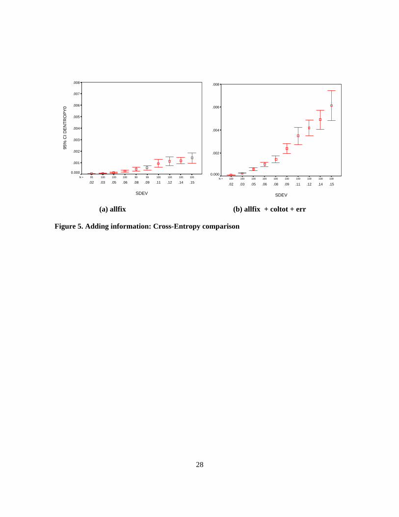
The cross-entropy measures reflect how much the information we have introduced has

shifted our solution estimates away from the inconsistent prior, while also accounting for the

imprecision of the moments assumed to be measured with error. Intuition suggests that if the

information constraints are binding, the distance from the prior will increase; if none are binding,

then the cross entropy (CE) distance will be zero. That is, there exists a y, such that Ay = y . In

our Core case without any constraints on the y other than that column and row sums must be

equal, a solution can be found without changing the column coefficients, as indicated by a CE

measure of zero.15 We observe that, as more information is imposed, the CE measure increases as

expected (Figure 5a and 5b).

<<Figure 5>>

7. Conclusion

The cross entropy (CE) approach provides a flexible and powerful method for estimating

a social accounting matrix (SAM) when dealing with scattered and inconsistent data. The method

represents a considerable extension and generalization of the standard RAS method, which

assumes that one starts from a consistent prior SAM and has knowledge only about new row and

column totals. The CE framework allows a wide range of prior information to be used efficiently

in estimation. Drawing on information theory, the cross-entropy approach is “efficient” in that it

uses all available information, but only that information—no assumed information is injected

15 The CE measure associated with the error term is zero for the Core and AllFix cases because the error term is set to zero and the column totals are free to vary, so no binding constraint is imposed.

19

into the estimation procedure.The prior information can be in a variety of forms, including linear

and nonlinear inequalities, errors in equations, and measurement error (using an error-in-

variables formulation). One also need not start from a balanced or consistent SAM. The results

from a variety of Monte Carlo experiments demonstrate the power of the CE approach and

provide measures of the gains from incorporating a wide range of information from a variety of

sources to improve our estimation of the SAM parameters.

20

References

Arndt, C., A. Cruz, H. Jensen, S. Robinson, and F. Tarp (1997) A Social Accounting Matrix for Mozambique: Base Year 1994, Institute of Economics, University of Copenhagen. Bacharach, Michael (1970) Biproportional Matrices and Input-Output Change (Cambridge University Press. University of Cambridge, No. 16 Department of Applied Economics). Barker, T., F. van der Ploeg, and M. Weale (1984) “A Balance System of National Accounts for

the United Kingdom, Review of Income and Wealth, 30, pp. 461-485. Brooke, A., D. Kendrick, A. Meeraus, and R. Raman (1998) GAMS a User's Guide (GAMS Development Corporation, Washington D.C.). Byron, Ray P. (1978) The Estimation of Large Social Account Matrices, Journal of the Royal

Statistical Society, 141, Part 3, p. 359-367. Gilchrist, Donald A. and Larry V. St Louis (1999) Completing Input-Output Tables using Partial

Information, with an Application to Canadian Data, Economic Systems Research, Vol. 11, No. 2, pp. 185-193.

Golan, Amos, George Judge, and Douglas Miller (1996) Maximum Entropy Econometrics, Robust Estimation with Limited Data (John Wiley & Sons). Golan, Amos, George Judge, and Sherman Robinson (1994) Recovering Information from Incomplete or Partial Multisectoral Economic Data, Review of Economics and Statistics 76, 541-9. Golan, Amos, and Stephen J. Vogel (1997) Estimation of Stationary and Non-Stationary Accounting Matrix Coefficients With Structural and Supply-Side Information, ERS/USDA. Unpublished. Harrigan, Frank J. (1990) The Reconciliation of Inconsistent Economic Data: the Information

Gain, Economics Systems Research 2:1, pp. 17-25. Harrigan, Frank J. and J.T. Buchanan (1984) A Quadratic Programming Approach to the

Estimation and Simulation of Input-Output Tables, Journal of Regional Science 24, pp. 339-358.

Harrigan, Frank J. and I. McNicoll (1986) Data Use and the Simulation of Regional Input-Output

Matrices, Environment and Planning A, 18, pp. 1061-1076. Judge, G., R. Hill, W. Griffiths, H. Lutkepohl, and T. Lee (1988) Introduction to The Theory and

Practice of Econometrics (John Wiley & Sons).

21

Kapur, Jagat Narain, Hiremaglur K. Kesavan (1992) Entropy Optimization Principles with Applications (Academic Press). Kullback, S. and R. A. Leibler (1951) On Information and Sufficiency, Ann. Math. Stat. 4, 99- 111. McDougall, Robert, (1999) Entropy Theory and RAS are Friends (http://www.sjfi.dk/gtap/papers /McDougall.pdf) Pindyck, Robert S., and Daniel L. Rubinfeld (1991) Econometric Models & Economic Forecasts (McGraw Hill). Schneider, M. H., and S. A. Zenios (1990) A comparative study of algorithms for matrix balancing, Operations Research 38, 439-55. Shannon, C. E. (1948) A mathematical theory of communication, Bell System Technical Journal 27, 379-423. Theil, Henri (1967) Economics and Information Theory (North-Holland). Toh, Mun-Heng (1998) The RAS Approach in Updating Input-Output Matrices: An Instrumental

Variable Interpretation and Analysis of Structural Change, Economic Systems Research, Vol. 10, No. 1, pp. 63-78.

Van der Ploeg, F. (1982) Reliability and the Adjustment of Sequences of Large Economic

Accounting Matrices, Journal of the Royal Statistical Society, 145, Part 2, pp. 169-194. Zellner, A. (1988) Optimal Information Processing and Bayes Theorem, American Statistician 42, 278-84. Zellner, A. (1990) Bayesian Methods and Entropy in Economics and Econometrics, In: W. T.

Grandy and L. H. Shick (eds) Maximum Entropy and Bayesian Methods (Kluwer, Dordrecht).

22

Table 1. A National SAM

Expenditure

Receipts Activity Commodity Factors Institutions World

Activity Domestic

sales

Commodity Intermediate

inputs

Final demand Exports

Factors Value added

(wages/rentals)

Institutions Indirect taxes Tariffs Factor income

Capital inflow

World Imports

Totals Total costs Total

absorption Total factor

income Gross domestic

income

Foreign exchange

inflow

23

Table 2. 1994 SAM for Mozambique (millions of 1994 Meticais)

Expenditure

Receipts (1) (2) (3) (4) (5) (6) (7) (8) (9) (10) (11) (12) Totals

(1) Agr. activity 25.14 30.50 55.64

(2) Non-agr. activity 12.46 206.28 2.14 220.88

(3) Agr. Commodity 1.58 13.42 20.12 0.00 0.09 8.58 43.79

(4) Non-agr. Commodity 7.24 98.86 86.72 16.77 0.00 33.94 33.03 24.13 300.69

(5) Factors 47.01 108.74 155.75

(6) Enterprises 62.86 62.86

(7) Households 91.63 58.96 1.33 3.46 155.38

(8) Rec. govt.* 0.94 9.88 1.26 2.41 2.49 22.53

(9) Indirect tax -0.19 -0.14 0.24 5.64 5.55

(10) Govt. investment 22.94 22.94

(11) Private investment 1.49 13.41 4.43 -11.00 24.79 33.12

(12) Rest of the world 5.01 78.89 83.90

Totals 55.64 220.88 43.79 300.69 155.75 62.86 155.38 22.53 5.55 22.94 33.12 83.90 1163.02

Source Arndt, C. et al., 1997 * Recurrent government expenditures

24

(a) flows (b) coefficients

Figure 1. Comparison of the root mean square deviation relative to the initial SAM (for flows and coefficients).

RMS deviation for flows (RAS)

.6.5.4.3.2.1

RM

S d

evia

tion

for

flow

s (e

ntro

py)

.6

.5

.4

.3

.2

.1

RMS deviation for Coefficients (RAS)

.06.05.04.03.02.010.00

RM

S d

ev. f

or c

oeffi

cien

ts (

Ent

ropy

)

.06

.05

.04

.03

.02

.01

0.00

25

flows (b) coefficients

Figure 2. Basic Estimation: 95% confidence interval for root mean square error after balancing with entropy method (relative to unperturbed SAM).

100100100100100100100100100100N =

SDEV

.15.14.12.11.09.08.06.05.03.02

95%

CI R

MS

E

.4

.3

.2

.1

0.0100100100100100100100100100100N =

SDEV

.15.14.12.11.09.08.06.05.03.02

95%

CI C

RM

SE

.014

.012

.010

.008

.006

.004

.002

0.000

26

(a) allfix (b) allfix + totals with error

Figure 3. Adding information: 95% confidence interval for root mean square error of flows after balancing with entropy method (relative to unperturbed SAM) .

100100100100100100100100100100N =

SDEV

.15.14.12.11.09.08.06.05.03.02

95%

CI R

MS

E

.4

.3

.2

.1

0.0100100100100100100100100100100N =

SDEV

.15.14.12.11.09.08.06.05.03.02

95%

CI R

MS

E

.4

.3

.2

.1

0.0

27

(a) allfix (b) allfix + totals with error

Figure 4. Adding information: 95% confidence interval for root mean square error of coefficients after balancing with entropy method (relative to unperturbed SAM)

100100100100100100100100100100N =

SDEV

.15.14.12.11.09.08.06.05.03.02

95%

CI C

RM

SE

.014

.012

.010

.008

.006

.004

.002

0.000100100100100100100100100100100N =

SDEV

.15.14.12.11.09.08.06.05.03.02

95%

CI C

RM

SE

.014

.012

.010

.008

.006

.004

.002

0.000

28

(a) allfix (b) allfix + coltot + err

Figure 5. Adding information: Cross-Entropy comparison

100100100100100100100100100100N =

SDEV

.15.14.12.11.09.08.06.05.03.02

95%

CI D

EN

TR

OP

Y0

.008

.006

.004

.002

0.000100100100100999910010010095N =

SDEV

.15.14.12.11.09.08.06.05.03.02

95%

CI D

EN

TR

OP

Y0

.008

.007

.006

.005

.004

.003

.002

.001

0.000

IFPRI Trade and Macroeconomics Division

TMD Discussion Papers marked with an “*” are MERRISA-related. Copies can be obtained by calling Maria Cohan at 202-862-5627 or e-mail: m.cohan@cgiar.org

List of Discussion Papers

No. 1 - "Land, Water, and Agriculture in Egypt: The Economywide Impact of Policy Reform" by Sherman Robinson and Clemen Gehlhar (January 1995)

No. 2 - "Price Competitiveness and Variability in Egyptian Cotton: Effects of Sectoral and Economywide Policies" by Romeo M. Bautista and Clemen Gehlhar (January 1995)

No. 3 - "International Trade, Regional Integration and Food Security in the Middle East" by Dean A. DeRosa (January 1995)

No. 4 - "The Green Revolution in a Macroeconomic Perspective: The Philippine Case" by Romeo M. Bautista (May 1995)

No. 5 - "Macro and Micro Effects of Subsidy Cuts: A Short-Run CGE Analysis for Egypt" by Hans Löfgren (May 1995)

No. 6 - "On the Production Economics of Cattle" by Yair Mundlak, He Huang and Edgardo

Favaro (May 1995)

No. 7 - "The Cost of Managing with Less: Cutting Water Subsidies and Supplies in Egypt's

Agriculture" by Hans Löfgren (July 1995, Revised April 1996)

No. 8 - "The Impact of the Mexican Crisis on Trade, Agriculture and Migration" by Sherman Robinson, Mary Burfisher and Karen Thierfelder (September 1995)

No. 9 - "The Trade-Wage Debate in a Model with Nontraded Goods: Making Room for Labor Economists in Trade Theory" by Sherman Robinson and Karen Thierfelder (Revised March 1996)

No. 10 - "Macroeconomic Adjustment and Agricultural Performance in Southern Africa: A Quantitative Overview" by Romeo M. Bautista (February 1996)

No. 11 - "Tiger or Turtle? Exploring Alternative Futures for Egypt to 2020" by Hans Löfgren, Sherman Robinson and David Nygaard (August 1996)

No. 12 - "Water and Land in South Africa: Economywide Impacts of Reform - A Case Study for the Olifants River" by Natasha Mukherjee (July 1996)

IFPRI Trade and Macroeconomics Division

TMD Discussion Papers marked with an “*” are MERRISA-related. Copies can be obtained by calling Maria Cohan at 202-862-5627 or e-mail: m.cohan@cgiar.org

No. 13 - "Agriculture and the New Industrial Revolution in Asia" by Romeo M. Bautista and Dean A. DeRosa (September 1996)

No. 14 - "Income and Equity Effects of Crop Productivity Growth Under Alternative Foreign Trade Regimes: A CGE Analysis for the Philippines" by Romeo M. Bautista and Sherman Robinson (September 1996)

No. 15 - "Southern Africa: Economic Structure, Trade, and Regional Integration" by Natasha Mukherjee and Sherman Robinson (October 1996)

No. 16 - "The 1990's Global Grain Situation and its Impact on the Food Security of Selected Developing Countries" by Mark Friedberg and Marcelle Thomas (February 1997)

No. 17 - "Rural Development in Morocco: Alternative Scenarios to the Year 2000" by Hans Löfgren, Rachid Doukkali, Hassan Serghini and Sherman Robinson (February 1997)

No. 18 - "Evaluating the Effects of Domestic Policies and External Factors on the Price Competitiveness of Indonesian Crops: Cassava, Soybean, Corn, and Sugarcane" by Romeo M. Bautista, Nu Nu San, Dewa Swastika, Sjaiful Bachri and Hermanto (June 1997)

No. 19 - "Rice Price Policies in Indonesia: A Computable General Equilibrium (CGE) Analysis" by Sherman Robinson, Moataz El-Said, Nu Nu San, Achmad Suryana, Hermanto, Dewa Swastika and Sjaiful Bahri (June 1997)

No. 20 - "The Mixed-Complementarity Approach to Specifying Agricultural Supply in Computable General Equilibrium Models" by Hans Löfgren and Sherman Robinson (August 1997)

No. 21 - "Estimating a Social Accounting Matrix Using Entropy Difference Methods" by Sherman Robinson and Moataz-El-Said (September 1997)

No. 22 - "Income Effects of Alternative Trade Policy Adjustments on Philippine Rural

Households: A General Equilibrium Analysis" by Romeo M. Bautista and Marcelle Thomas (October 1997)

No. 23 - "South American Wheat Markets and MERCOSUR" by Eugenio Díaz-Bonilla (November 1997)

IFPRI Trade and Macroeconomics Division

TMD Discussion Papers marked with an “*” are MERRISA-related. Copies can be obtained by calling Maria Cohan at 202-862-5627 or e-mail: m.cohan@cgiar.org

No. 24 - "Changes in Latin American Agricultural Markets" by Lucio Reca and Eugenio Díaz-Bonilla (November 1997)

No. 25* - "Policy Bias and Agriculture: Partial and General Equilibrium Measures" by Romeo M. Bautista, Sherman Robinson, Finn Tarp and Peter Wobst (May 1998)

No. 26 - "Estimating Income Mobility in Colombia Using Maximum Entropy Econometrics" by Samuel Morley, Sherman Robinson and Rebecca Harris (Revised February 1999)

No. 27 - "Rice Policy, Trade, and Exchange Rate Changes in Indonesia: A General Equilibrium Analysis" by Sherman Robinson, Moataz El-Said and Nu Nu San (June 1998)

No. 28* - "Social Accounting Matrices for Mozambique - 1994 and 1995" by Channing Arndt, Antonio Cruz, Henning Tarp Jensen, Sherman Robinson and Finn Tarp (July 1998)

No. 29* - "Agriculture and Macroeconomic Reforms in Zimbabwe: A Political-Economy Perspective" by Kay Muir-Leresche (August 1998)

No. 30* - "A 1992 Social Accounting Matrix (SAM) for Tanzania" by Peter Wobst (August 1998)

No. 31* - "Agricultural Growth Linkages in Zimbabwe: Income and Equity Effects" by Romeo M. Bautista and Marcelle Thomas (September 1998)

No. 32* - "Does Trade Liberalization Enhance Income Growth and Equity in Zimbabwe? The

Role of Complementary Polices" by Romeo M.Bautista, Hans Lofgren and Marcelle Thomas (September 1998)

No. 33 - "Estimating a Social Accounting Matrix Using Cross Entropy Methods" by Sherman

Robinson, Andrea Cattaneo and Moataz El-Said (October 1998) No. 34 - "Trade Liberalization and Regional Integration: The Search for Large Numbers" by

Sherman Robinson and Karen Thierfelder (January 1999) No. 35 - "Spatial Networks in Multi-Region Computable General Equilibrium Models" by

Hans Löfgren and Sherman Robinson (January 1999) No. 36* - "A 1991 Social Accounting Matrix (SAM) for Zimbabwe" by Marcelle Thomas, and

Romeo M. Bautista (January 1999) No. 37 - "To Trade or not to Trade: Non-Separable Farm Household Models in Partial and

General Equilibrium" by Hans Löfgren and Sherman Robinson (January 1999)

IFPRI Trade and Macroeconomics Division

TMD Discussion Papers marked with an “*” are MERRISA-related. Copies can be obtained by calling Maria Cohan at 202-862-5627 or e-mail: m.cohan@cgiar.org

No. 38 - "Trade Reform and the Poor in Morocco: A Rural-Urban General Equilibrium Analysis of Reduced Protection" by Hans Löfgren (January 1999)

No. 39 - " A Note on Taxes, Prices, Wages, and Welfare in General Equilibrium Models" by Sherman Robinson and Karen Thierfelder (January 1999)

No. 40 - "Parameter Estimation for a Computable General Equilibrium Model: A Maximum Entropy Approach" by Channing Arndt, Sherman Robinson and Finn Tarp (February 1999)

No. 41 - "Trade Liberalization and Complementary Domestic Policies: A Rural-Urban General Equilibrium Analysis of Morocco" by Hans Löfgren, Moataz El-Said and Sherman Robinson (April 1999)

No. 42 - "Alternative Industrial Development Paths for Indonesia: SAM and CGE Analysis" by Romeo M. Bautista, Sherman Robinson and Moataz El-Said (May 1999)

No. 43* - "Marketing Margins and Agricultural Technology in Mozambique" by Channing

Arndt, Henning Tarp Jensen, Sherman Robinson and Finn Tarp (July 1999)

No. 44 - "The Distributional Impact of Macroeconomic Shocks in Mexico: Threshold Effects

in a Multi-Region CGE Model" by Rebecca Lee Harris (July 1999)

No. 45 - "Economic Growth and Poverty Reduction in Indochina: Lessons From East Asia" by

Romeo M. Bautista (September 1999)

No. 46* - "After the Negotiations: Assessing the Impact of Free Trade Agreements in Southern

Africa" by Jeffrey D. Lewis, Sherman Robinson and Karen Thierfelder (September 1999)

No. 47* - "Impediments to Agricultural Growth in Zambia" by Rainer Wichern, Ulrich Hausner

and Dennis K. Chiwele (September 1999)

No. 48 - "A General Equilibrium Analysis of Alternative Scenarios for Food Subsidy Reform

in Egypt" by Hans Lofgren and Moataz El-Said (September 1999)

No. 49*- “ A 1995 Social Accounting Matrix for Zambia” by Ulrich Hausner (September 1999)

No. 50 - “Reconciling Household Surveys and National Accounts Data Using a Cross Entropy

-Sophie Robilliard and Sherman Robinson (November 1999)

IFPRI Trade and Macroeconomics Division

TMD Discussion Papers marked with an “*” are MERRISA-related. Copies can be obtained by calling Maria Cohan at 202-862-5627 or e-mail: m.cohan@cgiar.org

No. 51 - “Agriculture-Based Development: A SAM Perspective on Central Viet Nam” by Romeo M. Bautista (January 2000)

No. 52 - “Structural Adjustment, Agriculture, and Deforestation in the Sumatera Regional

Economy” by Nu Nu San, Hans Löfgren and Sherman Robinson (March 2000)

No. 53 - “Empirical Models, Rules, and Optimization: Turning Positive Economics on its

Head” by Andrea Cattaneo and Sherman Robinson (April 2000)

No. 54 - “Small Countries and the Case for Regionalism vs. Multilateralism” by Mary E. Burfisher, Sherman Robinson and Karen Thierfelder (May 2000)

No. 55 - “Genetic Engineering and Trade: Panacea or Dilemma for Developing Countries” by Chantal Pohl Nielsen, Sherman Robinson and Karen Thierfelder

(May 2000)

No. 56 - “An International, Multi-region General Equilibrium Model of Agricultural Trade Liberalization in the South Mediterranean NIC’s, Turkey, and the European Union” by Ali Bayar, Xinshen Diao, A. Erinc Yeldan (May 2000)

No. 57* - “Macroeconomic and Agricultural Reforms in Zimbabwe: Policy Complementarities

Toward Equitable Growth” by Romeo M. Bautista and Marcelle Thomas (June 2000)

No. 58 - “Updating and Estimating a Social Accounting Matrix Using Cross Entropy Methods ” by Sherman Robinson, Andrea Cattaneo and Moataz El-Said (August 2000)