Unspanned macroeconomic factors in the yield curve

Laura CoroneoUniversity of York

Domenico GiannoneFederal Reserve Bank of New York

CEPR, ECARES and LUISS

Michele ModugnoBoard of Governors of the Federal Reserve System

April 3, 2015

Abstract

In this paper, we extract common factors from a cross-section of U.S. macro-variables and Trea-sury zero-coupon yields. We find that two macroeconomic factors have an important predictivecontent for government bond yields and excess returns. These factors are not spanned by thecross-section of yields and are well proxied by economic growth and real interest rates.

JEL classification codes: C33, C53, E43, E44, G12.

Keywords: Yield Curve; Government Bonds; Dynamic Factor Models; Forecasting.

We thank Carlo Altavilla, Andrea Carriero, Valentina Corradi, Rachel Griffith, Matteo Luciani, Emanuel

Monch, Denise Osborn, Jean-Charles Wijnandts, the Editor Shakeeb Khan, the Associate Editor and referees

for useful comments. We also thank seminar participants at HEC Montreal, Federal Reserve Bank of Saint

Louis, the 2012 International Conference on Computing in Economics and Finance, the 2012 European

Meetings of the Econometric Society, the University of York, the cemmap, UCL and Bank of England

workshop on Frontiers of Macroeconometrics and the 2013 Vienna Workshop on High Dimensional Time

Series. Any remaining errors are our own. Laura Coroneo gratefully acknowledges the support of the ESRC

grant ES/K001345/1 and Domenico Giannone was supported by the “Action de recherche concerte” contract

ARC-AUWB/2010-15/ULB-11 and by the IAP research network grant nr. P7/06 of the Belgian government

(Belgian Science Policy). The opinions in this paper are those of the authors and do not necessarily reflect

the views of either the Board of Governors of the Federal Reserve System or Federal Reserve Bank of New

York, or the Federal Reserve System.

1 Introduction

Government bond yields with different maturities and macroeconomic variables are both character-

ized by a high degree of comovement, indicating that the bulk of their dynamics is driven by a few

common forces. Three common factors, usually interpreted as the level, slope and curvature of the

yield curve, can explain changes and shifts of the entire cross-section of yields, see Litterman and

Scheinkman (1991). Although there is less consensus on the number and nature of macroeconomic

factors, two factors, one nominal and one real, summarize well the dynamics of a large variety of

macroeconomic indicators for the United States, see Sargent, Sims et al. (1977), Giannone, Reichlin

and Sala (2005) and Watson (2005).

Macroeconomic factors and yield curve factors are also characterized by a strong interaction.

The short end of the yield curve moves closely to the policy instrument under the direct control

of the central bank, which responds to changes in inflation, economic activity, or other economic

conditions, see Taylor (1993). The average level of the yield curve is usually associated with the in-

flation rate and the spread between long and short rates with temporary business cycles conditions,

see Diebold, Rudebusch and Aruoba (2006). For these reasons, macroeconomic information has

been shown to help forecasting future interest rates and excess bond returns, see Ang and Piazzesi

(2003), Monch (2008), De Pooter, Ravazzolo and Van Dijk (2007), Favero, Niu and Sala (2012) and

Ludvigson and Ng (2009).

In this paper, we aim at identifying the factors summarizing macroeconomic information that is

not spanned by the traditional yield curve factors. The economic literature so far has not addressed

this problem since in existing studies macroeconomic factors are either proxied by preselected

observable variables, see Bianchi, Mumtaz and Surico (2009), Dewachter and Lyrio (2006), Diebold

et al. (2006), Joslin, Priebsch and Singleton (2014), Rudebusch and Wu (2008), and Wright (2011),

or extracted from a large set of macroeconomic indicators and treated separately from the yield

curve factors, see Ang and Piazzesi (2003), Favero et al. (2012), Ludvigson and Ng (2009), Monch

(2008) and Monch (2012).

1

We estimate a macro-yield model that treats macroeconomic factors as unobservable compo-

nents that we extract simultaneously with the traditional yield curve factors. Following Diebold

and Li (2006) and Diebold and Rudebusch (2013), the factors affecting the yield curve are identified

by constraining the loadings to follow the smooth pattern proposed by Nelson and Siegel (1987).

More specifically, our empirical model is a Dynamic Factor Model (DFM) for Treasury zero-coupon

yields and a representative set of macroeconomic variables with restrictions on the factor loadings.

Following Doz, Giannone and Reichlin (2012) the model is estimated by quasi maximum likelihood,

i.e. we maximize the likelihood of a potentially miss-specified model. Precisely, the likelihood is

computed assuming that the dynamic factor model is Gaussian and exact (the idiosyncratic errors

are assumed to be cross-sectionally orthogonal). Doz et al. (2012) have shown that, when estima-

tion is carried out with a large number of highly collinear variable, the estimator is consistent and

robust to non Gaussianity and to weak correlation among idiosyncratic components.

Using monthly U.S. data from January 1970 to December 2008, we find that a significant

component of macroeconomic information is not captured by the yield curve factors and, at the

same time, is unspanned by the yield curve, in the sense that it does not affect contemporaneously

the cross-section of yields. The unspanned macroeconomic information is driven by two factors

that are well proxied by economic growth and real interest rates. These factors have substantial

predictive information for bond yields and excess bond returns, in spite of the fact that they do

not affect contemporaneously the shape of the yield curve. The macro-yields model explains up

to 55% of the variation in excess bond returns and outperforms all existing models in forecasting

bond yields and excess returns.

The paper is organized as follows. Section 2 presents the macro-yields model. Section 3 describes

the data, the estimation procedure and the information criteria used for model selection. Section

4 describes the empirical results and in-sample validation of the model. Section 5 assesses the

forecasting performance of the model in real time. Section 6 concludes.

2

2 The macro-yields model

We propose a dynamic factor model for the joint behavior of government bond yields and macroe-

conomic indicators. Bond yields at different maturities are driven by the traditional level, slope

and curvature factors. Macroeconomic variables load on the yield curve factors as well as on some

additional macro factors that capture the information in macroeconomic variables over and above

the yield curve factors. We assume that these additional macro factors do not provide any infor-

mation about the contemporaneous shape of the yield curve. According to this model, the level,

slope, and curvature factors are spanned by both the bond yields and macroeconomic variables.

The additional macro factors, instead, are contemporaneously loaded only by the macroeconomic

variables and, thus, are unspanned by the cross-section of the yields. The remaining of this section,

describes the model in details.

The cross section of bond yields is modeled using the Dynamic Nelson-Siegel framework of

Diebold and Li (2006). Denoting by yt the Ny × 1 vector of yields with Ny different maturities at

time t, we have

yt = ay + Γyy Fyt + vyt , (1)

where F yt is a 3 × 1 vector containing the latent yield-curve factors at time t, Γyy is a Ny × 3

matrix of factor loadings, and vyt is an Ny × 1 vector of idiosyncratic components. The yield curve

factors F yt are identified by constraining the factor loadings to follow the smooth pattern proposed

by Nelson and Siegel (1987) (hereafter NS)

ay = 0; Γ(τ)yy =

[1

1− e−λτ

λτ

1− e−λτ

λτ− e−λτ

]≡ Γ

(τ)NS , (2)

where Γ(τ)yy is the row of the matrix of factor loadings corresponding to the yield with maturity τ

months and λ is a decay parameter of the factor loadings. Diebold and Li (2006) show that this

functional form of the factor loadings, implies that the three yield curve factors can be interpreted

as the level, slope, and curvature of the yield curve. Indeed, the loading equal to one on the first

3

factor, for all maturities, implies that an increase in this factor increases all yields equally, shifting

the level of the yield curve. The loadings on the second factor are large for short maturities,

decaying to zero for the long ones. Accordingly, an increase in the second factor decreases the slope

of the yield curve. Loadings on the third factor are zero for the shortest and the longest maturities,

reaching the maximum for medium maturities. Therefore, an increase in this factor augments the

curvature of the yield curve. The specific shape of the loadings depends on the decay parameter λ,

which we calibrate to the value that maximizes the loading on the curvature factor for the yields

with maturity 30 months, as in Diebold and Li (2006).

Given these particular functional forms for the loadings on the three yield curve factors, one

can summarize movements in the term structure of interest rates into three factors which have a

clear-cut interpretation. The NS factors are just linear combinations of yields. The level factor can

be proxied by the long term yield, the slope by the spread between the long and short maturity yield

(first derivative) and the curvature by sum of the spreads between a medium and a long term yield,

and between a medium and the short term yield (second derivative), see Diebold and Li (2006).1

Due to its flexibility and parsimony, the NS model accurately fits the yield curve and performs

well in out-of-sample forecasting exercises, as shown by Diebold and Li (2006) and De Pooter et al.

(2007). For these reasons, fixed-income wealth managers in public organizations, investment banks

and central banks rely heavily on NS type of models to fit and forecast yield curves, see BIS (2005),

ECB (2008), Gurkaynak, Sack and Wright (2007) and Coroneo, Nyholm and Vidova-Koleva (2011).

Macroeconomic variables, are assumed to be potentially driven by two sources of co-movement,

the yield curve factors F yt and macro specific factors. Denoting by xt the Nx× 1 vector of macroe-

conomic variables at time t, we have

xt = ax + Γxy Fyt + Γxx F

xt + vxt , (3)

where F xt is an r × 1 vector of macroeconomic latent factors, Γxy is a Nx × 3 matrix of factor

1Similar proxies are used by Ang, Piazzesi and Wei (2006) and Duffee (2011a).

4

loadings on the yield curve factors, Γxx is a Nx × r matrix of factor loadings on the macro factors,

and vxt is an Nx × 1 vector of idiosyncratic components.

The yield curve and the macroeconomic factors are extracted by estimating (1) and (3) simul-

taneously

ytxt

=

0

ax

+

Γyy Γyx

Γxy Γxx

F ytF xt

+

vytvxt

, Γyy = ΓNS , Γyx = 0, (4)

where ΓNS is defined according to (2).

The joint dynamics of the yield curve and the macroeconomic factors follow a VAR(1)

F ytF xt

=

µyµx

+

Ayy Ayx

Axy Axx

F yt−1F xt−1

+

uytuxt

,

uytuxt

∼ N0,

Qyy Qyx

Qxy Qxx

. (5)

The idiosyncratic components collected in vt = [vyt vxt ]′ are modelled to follow independent

autoregressive processes

vt = Bvt−1 + ξt, ξt ∼ N(0, R) (6)

where B and R are diagonal matrices, implying that the common factors fully account for the joint

correlation of the observations. The residuals to the idiosyncratic components of the individual

variables, ξt, and the innovations driving the common factors, ut, are assumed to be normally

distributed and mutually independent. This assumptions implies that the common factors are not

allowed to react to variable specific shocks.

The assumptions of Gaussianity and of independence among idiosyncratic components might

be sources of miss-specification. It is hard to relax these restrictions since they are necessary

to retain parsimony, insure identification of the common and idiosyncratic components and limit

computational complexity. However, Doz et al. (2012) have shown that, if the factor structure is

strong, the Maximum Likelihood estimates are robust not only to non Gaussianity but also to the

presence of limited correlations among idiosyncratic components.

5

Allowing Γxy to be different from zero is crucial to insure that the macroeconomic factors F xt

capture only those source of co-movement in the macroeconomic variables that are not already

spanned by the yield curve factors. Existing studies, instead, have imposed a block-diagonal struc-

ture of the factor loadings (Γxy = 0 and Γyx = 0), either explicitly, as in Monch (2012), either

implicitly by extracting the macro factors exclusively from macroeconomic variables, as in Ludvig-

son and Ng (2009).

Assuming that macroeconomic factors do not provide any information about the contemporane-

ous shape of the yield curve (Γyx = 0) restricts the macroeconomic factors F xt to be unspanned not

only by the yield factors but also by the entire cross-section of yields. This restriction is expected

to be immaterial since, as stressed above, the yield factors F yt are notoriously effective at fitting

the entire yield curve.

In the remainder of the paper we will maintain the restriction Γyx = 0 and leave Γxy unrestricted,

unless otherwise mentioned.2

3 Estimation and preliminary results

3.1 Data

We use monthly U.S. Treasury zero-coupon yield curve data spanning the period January 1970

to December 2008. The bond yield data are taken from the Fama-Bliss dataset available from

the Center for Research in Securities Prices (CRSP) and contain observations on three months

and one through five-year zero coupon bond yields. The macroeconomic dataset consists of 14

macroeconomic variables, which include five inflation measures, seven real variables, the federal

funds rate and a money indicator. Appendix B contains a complete list of the macroeconomic

variables along with the transformation applied to ensure stationarity. Following Ang and Piazzesi

(2003), De Pooter et al. (2007), Diebold et al. (2006) and Monch (2008), we use annual growth

rates for all variables, except for capacity utilization, the federal funds rate, the unemployment rate

2Results for the block-diagonal model (Γxy = 0, Γyx = 0) and the unrestricted model (Γxy 6= 0) are availableupon request.

6

and the manufacturing index which we keep in levels.3

3.2 Estimation

Equations (4)–(6) describe a restricted state-space model with autocorrelated idiosyncratic compo-

nents for which maximum likelihood estimators of the parameters are not available in closed form.

Conditionally on the factors, the model reduces in a set of linear regressions. As consequence, the

Maximum Likelihood estimates can be easily computed using the Expectation Maximization (EM)

algorithm, as described in detail in Appendix A.4

We initialize the yield curve factors with the NS factors using the two-steps OLS procedure

introduced by Diebold and Li (2006). We then project the macroeconomic variables on the NS fac-

tors and use the principal components of the residuals of this regression to initialize the unspanned

macroeconomic factors. Γyy is restricted to be equal to the NS loadings. All the other parameters

are initialized with the OLS estimates obtained using the initial guesses of yield and macro factors

described above. Given the initial parameters, a new set of factors is obtained using the Kalman

smoother. If we stop at this stage, we have the two-step procedure of Doz, Giannone and Reichlin

(2011).5 Maximum Likelihood estimates are obtained by iterating these two steps until convergence

provided that OLS regressions are modified in order to take into account the fact that the common

factors are estimated.6

For comparison, we also estimate an only-yields model, which uses only the information con-

tained in the yields. This is a restricted version of the macro-yields model in equations (4)–(6) with

Qyx = Ayx = Γxy = 0 and can hence be estimated using the same procedure.

3Since the selection of variables has an element of arbitrariness, we have performed robustness checks with analternative databases constructed by Banbura, Giannone, Modugno and Reichlin (2012) that includes all the variablesthat are constantly monitored by market participants. Results, available upon request, show that the main findingsare confirmed.

4Using the Expectation Conditional Restricted Maximization (ECRM) algorithm is also possible to estimate λ,but, despite the increase in the computation burden, the empirical results remain qualitatively similar to thoseobtained by setting λ to the value that maximizes the loading of the the yields with maturity 30 months on thecurvature factor.

5Interestingly, using final or initial estimates delivers similar results (available upon request). This is not surprisingsince Doz et al. (2011) and Doz et al. (2012) show that, if the factor structure is strong, the two-step and the maximumlikelihood approach have similar properties, both asymptotically and in small sample.

6See Appendix A for details.

7

3.3 Model selection

The macro-yields model decomposes variations in yields and macroeconomic variables into yield

curve factors, unspanned macroeconomic factors and idiosyncratic noises. The yield curve factors

are identified as the NS factors which have a clear interpretation as level, slope, and curvature.

However, the true number of unspanned macroeconomic factors is unknown. We select the optimal

number of factors using an information criteria approach. The idea is to choose the number of

factors that maximizes the general fit of the model using a penalty function to account for the loss

in parsimony.

Bai and Ng (2002) derive information criteria to determine the number of factors in approximate

factor models when the factors are estimated by principal components. They also show that their

IC3 information criterion can be applied to any consistent estimator of the factors provided that the

penalty function is derived from the correct convergence rate. For the quasi-maximum likelihood

estimator, Doz et al. (2012) show that it converges to the true value at a rate equal to

C∗2NT = min

{√T ,

N

logN

}(7)

where N and T denote the cross-section and the time dimension, respectively. Thus, a modified

Bai and Ng (2002) information criterion that can be used to select the optimal number of factors

when estimation is performed by quasi-maximum likelihood is as follows

IC∗(s) = log(V (s, F(s))) + s g(N,T ), g(N,T ) =logC∗2NTC∗2NT

(8)

where s denotes the number of factors, F(s) are the estimated factors and V (s, F(s)) is the sum

of squared idiosyncratic components (divided by NT) when s factors are estimated. The penalty

function g(N,T ) is a function of both N and T and depends on C∗2NT , the convergence rate of the

estimator, in our case given by (7).

To select the number of factors in the macro-yields model, we estimate the macro-yields model

8

Table 1: Model selection

Number of factors IC∗ V

3 0.02 0.444 -0.03 0.315 -0.11 0.226 0.01 0.187 0.23 0.178 0.43 0.16

This table reports the information cri-terion IC∗, as shown in (8) and (7), andthe sum of the variance of the idiosyn-cratic components (divided by NT ), V ,when different numbers of factors areestimated.

in equations (4)–(6) allowing from three up to a total of eight factors, where the first three are

identified as the yield curve factors and the others are unspanned macro factors. Table 1 reports

the information criterion, as shown in Equation (8), and the sum of the variance of the idiosyncratic

components for these different specifications of the macro-yields model. The information criterion

selects the model with five factors, i.e. three yield curve factors plus two unspanned factors.

This is also confirmed by the fact that the strongest reduction in the sum of the variances of the

idiosyncratic components is obtained passing from the four to the five factors specification. Thus

our macro-yields model is a latent factor model with three factors that explain the cross-section of

yields and two unspanned macroeconomics factors.

4 In sample results

4.1 Model fit

Table 2 reports the share of variance of the macroeconomic variables explained by the macro-yields

factors. Results show that, as expected, the yield curve factors explain most of the variance of

the federal funds rate and the yields at different maturities. They also explain the part of the

variance of price indices, unemployment, nominal earnings, nominal consumption and money, in

9

Table 2: Cumulative variance of yields and macro variables explained by the macro-yields factors

Level Slope Curv UM1 UM2

Government bond yield with maturity 3 months 0.59 0.94 1.00 1.00 1.00Government bond yield with maturity 1 year 0.61 0.83 0.99 0.99 0.99Government bond yield with maturity 2 years 0.65 0.78 0.99 0.99 0.99Government bond yield with maturity 3 years 0.70 0.79 1.00 1.00 1.00Government bond yield with maturity 4 years 0.74 0.80 0.99 0.99 0.99Government bond yield with maturity 5 years 0.78 0.82 0.99 0.99 0.99Average Hourly Earnings: Total Private 0.07 0.29 0.33 0.33 0.67Consumer Price Index: All Items 0.19 0.48 0.48 0.50 0.85Real Disposable Personal Income 0.00 0.02 0.03 0.34 0.36Effective Federal Funds Rate 0.53 0.93 0.96 0.96 0.97House Sales - New One Family Houses 0.00 0.19 0.19 0.23 0.23Industrial Production Index 0.02 0.02 0.03 0.69 0.69M1 Money Stock 0.17 0.25 0.25 0.25 0.31ISM Manufacturing: PMI Composite Index (NAPM) 0.03 0.05 0.05 0.61 0.65Payments All Employees: Total nonfarm 0.00 0.02 0.10 0.70 0.70Personal Consumption Expenditures 0.16 0.23 0.33 0.46 0.78Producer Price Index: Crude Materials 0.03 0.14 0.14 0.20 0.43Producer Price Index: Finished Goods 0.03 0.32 0.32 0.33 0.80Capacity Utilization: Total Industry 0.02 0.16 0.21 0.63 0.64Civilian Unemployment Rate 0.44 0.54 0.55 0.65 0.68

This table reports the cumulative share of variance of yields and macro variables explained by the macro-yields factors. The first three columns refer to the yield curve factors (level, slope and curvature) and thelast two to the unspanned macroeconomic factors (UM1 and UM2).

10

line with previous studies, see Diebold et al. (2006). The first unspanned macro factor captures

the dynamics of industrial production and other real variables, while the second unspanned factor

mainly explains inflation and other nominal variables.7

Figure 1 displays the estimated factors of the macro-yields model. The top three plots report

the yield curve factors, while the bottom two refer to the unspanned factors. The estimated yield

curve factors of the macro-yields model are highly correlated with the NS factors, which we estimate

by ordinary least squares as in Diebold and Li (2006) and report in dashed red lines in the top

plots. The differences between the NS factors and the first three macro-yields factors are due to the

fact that, in the macro-yields model, the yield curve factors are common to both yield curve and

macroeconomic variables. In fact, in the macro-yields model, we extract the yield curve factors from

both yields and macroeconomic variables and impose the NS restrictions on the factors loadings

of the yields to identify them as yield curve factors. The two bottom plots of Figure 1 show the

unspanned macro factors. The bottom left plot reports the first unspanned macro factor along

with the industrial production index, while the bottom right plot reports the second unspanned

macroeconomic factor along with the real interest rate (computed as the difference between the

federal funds rate and the consumer price index). As it is clear from the plots, the first unspanned

macroeconomic factor closely tracks the industrial production index, with a correlation of 90%, and

the second unspanned macroeconomic factor proxies the real interest, with a correlation of 74%.

This is in line with the fact that, as reported in Table 2, the first unspanned macroeconomic factor

explains mainly measures of real economic activity, while nominal variables are explained partly

by the yield curve factors and partly by the second unspanned factor. We can thus conclude that

the macro-yields models identifies two unspanned macroeconomic factors: real economic activity

and real interest rate. In the next Section we assess the quantitative importance of the unspanned

7The two macroeconomic factors are not identified since any transformation HF xt , with H non-singular, gives anobservationally equivalent model. In order to achieve identification additional restrictions are required. We do notimpose such restrictions and the EM algorithm converges to the Maximum Likelihood solution that is ”close” to theinitialisation, i.e. the principal components of the residuals of the macro variables after regressing them on the NSfactors. Identification can be achieved by assuming that the first macro factor has a loading of one for industrialproduction, and that the second macro factor has a loading of one for CPI and is not loaded by IP. Once we imposethis restriction, results, available upon request, do not change.

11

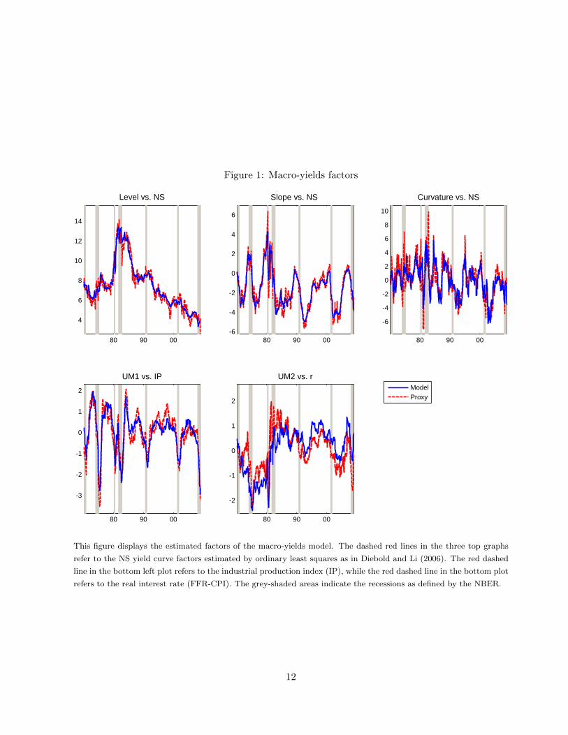
Figure 1: Macro-yields factors

80 90 00

4

6

8

10

12

14

Level vs. NS

80 90 00-6

-4

-2

0

2

4

6

Slope vs. NS

80 90 00

-6

-4

-2

0

2

4

6

8

10

Curvature vs. NS

80 90 00

-3

-2

-1

0

1

2

UM1 vs. IP

Model

Proxy

80 90 00

-2

-1

0

1

2

UM2 vs. r

This figure displays the estimated factors of the macro-yields model. The dashed red lines in the three top graphs

refer to the NS yield curve factors estimated by ordinary least squares as in Diebold and Li (2006). The red dashed

line in the bottom left plot refers to the industrial production index (IP), while the red dashed line in the bottom plot

refers to the real interest rate (FFR-CPI). The grey-shaded areas indicate the recessions as defined by the NBER.

12

macroeconomic factors in explaining bond risk premia.

4.2 Bond risk premia

The bond risk premium measures the compensation required by risk averse investors to hold long-

term government bonds for facing capital loss risk, if the bond is sold before maturity.

Long-term yields are determined by market expectations for the short rates over the holding

period of the long-term asset plus a yield risk premium. Assuming a minimum investment horizon

of one year, we have

y(τ)t =

( τ12

)−1 ∑i=0,12,...,τ−12

Et[y(12)t+i ] + yrp

(τ)t . (9)

An alternative measure for the bond risk premium can be obtained by looking at bond returns.

The one-year holding period bond return for a bond with maturity τ months is the return of buying

a bond with τ months to maturity at time t, selling it one year later, at time t+ 12, as a bond with

τ − 12 months to maturity, i.e.,

r(τ)t+12 = −(τ − 12)y

(τ−12)t+12 + τy

(τ)t . (10)

The expected one-year holding period return on long term bonds equals the expected return on the

short term bond plus the return risk premium

Et[r(τ)t+12] = y

(12)t + rrp

(τ)t , (11)

accordingly the return risk premium is the one-year expected return in excess of the one-year rate

rrp(τ)t = Et[r

(τ)t+12]− y

(12)t ≡ Et[rx(τ)t+12]. (12)

13

The relation between the return risk premium and the yield risk premium is as follows

yrp(τ)t =

1

τEt

[rrp

(τ)t + rrp

(τ−12)t+12 + . . .+ rrp

(24)t+τ−24

], (13)

which means that the yield risk premium is the average of expected future return risk premia of

declining maturity. This implies that the statements in Equations (9) and (11) are equivalent, if

one equation holds with zero (constant) bond risk premium, the other equation holds with zero

(constant) bond risk premium as well.

The expectations hypothesis of the term structure of interest rates states that the yield risk

premium is constant. This implies that expected excess returns are time invariant and, thus, excess

bond returns should not be predictable with variables in the information set at time t. However, the

expectations hypothesis has been empirically rejected since Fama and Bliss (1987) and Campbell

and Shiller (1991). They find that excess returns can be predicted by forward rate spreads and by

yield spreads, respectively. More recent evidence by Cochrane and Piazzesi (2005) shows that a

linear combination of forward rates (the CP factor) explains between 30% and 35% of the variation

in expected excess bond returns. Moreover, Ludvigson and Ng (2009) find that macroeconomic

factors constructed as linear and non-linear combinations of principal components extracted from

a large data-set of macroeconomic variables (the LN factor) have important forecasting power for

future excess returns on U.S. government bonds, above and beyond the predictive power contained

in forward rates and yield spreads. Cooper and Priestley (2009) also find that the output gap has

in-sample and out-of-sample predictive power for U.S. excess bond returns.

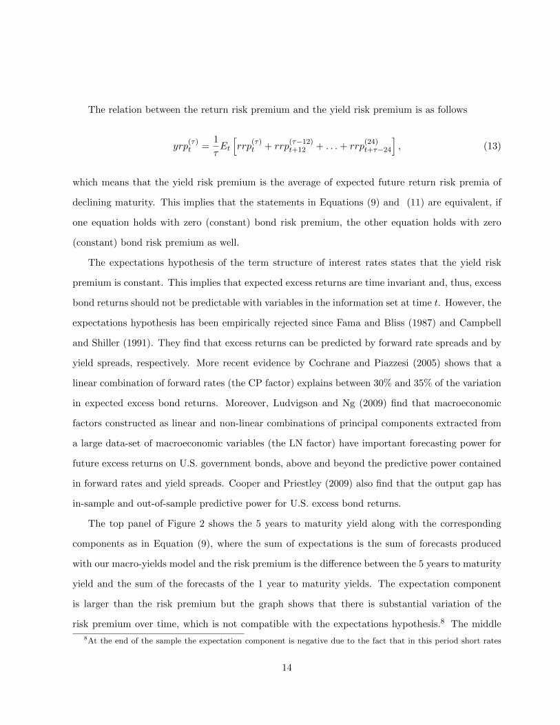
The top panel of Figure 2 shows the 5 years to maturity yield along with the corresponding

components as in Equation (9), where the sum of expectations is the sum of forecasts produced

with our macro-yields model and the risk premium is the difference between the 5 years to maturity

yield and the sum of the forecasts of the 1 year to maturity yields. The expectation component

is larger than the risk premium but the graph shows that there is substantial variation of the

risk premium over time, which is not compatible with the expectations hypothesis.8 The middle

8At the end of the sample the expectation component is negative due to the fact that in this period short rates

14

Figure 2: Yield risk premium, 5-year bond

72 75 77 80 82 85 87 90 92 95 97 00 02 05 07

0

5

10

15

Yield Expectations MY Risk Premium MY

72 75 77 80 82 85 87 90 92 95 97 00 02 05 07

-2

0

2

4

Risk Premium MY IP Growth

72 75 77 80 82 85 87 90 92 95 97 00 02 05 07

-1

0

1

2

3

4

Risk Premium MY Risk Premium OY

This figure displays the yield risk premium using the 5 years to maturity bond. The top panel shows the 5 years

to maturity yield (red dashed line) along with the corresponding expectation (green dot-dashed line) and the yield

risk premium (blue line) components, computed as in Equation (9) using the macro-yields model. The middle

panel reports the yield risk premium according to the macro-yields model (blue line) and the standardized industrial

production growth (red dashed line). The bottom plot shows the yield risk premium obtained from the macro-yields

model (blue line) and the only-yields model (red dashed line). The grey-shaded areas indicate the recessions as

defined by the NBER.

15

graph plots the risk premium against the industrial production index growth and it reveals that the

yield risk premium obtained from the macro-yields model displays a clear counter-cyclical pattern.

Its correlation with the industrial production index growth is -0.33. This is consistent with the

fact that investors want to be compensated for bearing risks related to recessions. Conversely, the

bottom graph in Figure 2, shows the risk premium obtained from the only-yields model. This model

delivers an acyclical risk premium, with a correlation of only -0.07 with the industrial production

index growth. This indicates that using macro variables greatly improves the estimates of the risk

premium.

Given that, as shown in Equation (13), the yield risk premium is the average of expected future

return risk premia of declining maturity, we analyze the predictive ability of the macro-yields model

for excess returns and compare it with the predictions of the only-yields model. We also compare

our results with predictions obtained using the CP factor, the LN factor and the CP and LN factors

combined.

We implement predictive regressions for the CP and LN factors by regressing excess bond

returns on the predictive factors Xt = {CPt, LNt} , as follows

rx(τ)t+12 = βXt + ε

(τ)t+12. (14)

We construct the predictive factors Xt by pooling the predictive regression for the individual ma-

turities

rxt+12 = γxt + εt+12, (15)

where rxt+12 = 14

∑τ=24,36,48,60 rx

(τ)t+12 and xt contains the predictor variables. To construct the

CP factor we use the following predictor variables xCPt = [1, y(12)t , f

(24)t , . . . , f

(60)t ], where f

(τ)t

denotes the τ -month forward rate.9 We estimate equation (15) using xCPt as predictor variables

reached the zero lower bound. Our macro-yields model does not impose a zero-lower bound to the predicted yields,but one could interpret the negative expectation component as a shadow rate.

9The τ -month forward rate for loans between time t+ τ − 12 and t+ τ is defined as

f(τ)t = −(τ − 12)y

(τ−12)t + τy

(τ)t .

16

Table 3: In-sample fit of excess bond returns

Maturity MY OY CP LN LN+CP

2y 0.55 0.12 0.22 0.33 0.413y 0.53 0.12 0.24 0.33 0.434y 0.50 0.14 0.27 0.32 0.435y 0.46 0.15 0.24 0.30 0.40

This table reports the R2 for one-year ahead one yearholding period excess bond returns from different mod-els. The columns MY and OY refer to the model-implied expected excess bond returns from the macro-yields model (MY) and the only-yields model (OY) re-spectively. The columns CP, LN and CP+LN referto the predictive regression using the Cochrane andPiazzesi (2005) factor (CP), the Ludvigson and Ng(2009) factor (LN), and both the Cochrane and Pi-azzesi (2005) and the Ludvigson and Ng (2009) factorsjointly.

and construct the CP factor as CPt = γCPxCPt . To construct the LN factor, we use as predictor

variables xLNt = [1, PC1t, . . . , PC8t, PC13t ], where PC denotes principal components extracted

from a large dataset of 131 macroeconomic data series.10 We then estimate equation (15) using

xLNt as predictor variables and construct the LN factor as LNt = γLNxLNt .

Notice that the LN factors are constructed aggregating principal components extracted from a

set of macroeconomic and financial variables without imposing that they are unspanned by the cross

section of the yields similarly to the factors extracted by assuming a block-diagonal structure on

the factor loadings. As a consequence, those factors duplicate information that is already spanned

by the yield factors.

Results in Table 3 show that the macro-yields model explains about 46-55% of the variation

of one-year ahead excess returns, while the only-yields model can explain only the 12-15% of

the variation of the one-year ahead excess returns. Table 3 reports also the R-squared from the

predictive regressions of excess bond returns on the CP and the LN factors. Results show that the

CP factor explains 22-27% of the variation in one-year ahead excess returns, slightly lower than

10The 131 macroeconomic data series used to construct the LN factor have been downloaded from Sydney C.Ludvigson’s website at http://www.econ.nyu.edu/user/ludvigsons/Data&ReplicationFiles.zip.

17

the value reported in Cochrane and Piazzesi (2005). This is due to the fact that our predictive

regressions are estimated on a more updated sample, and the performance of the CP factor has

deteriorated over time, as also shown by Thornton and Valente (2012). The LN factors explain a

third of the variation of future excess bond returns, while the CP and LN factors jointly explain

40-43% of the variation in one-year ahead excess bond returns, lower than what is explained by our

macro-yields model. We can thus conclude that, in-sample, the macro-yields model outperforms

the CP and the LN factors even combined.

Figure 3 shows the predicted and realized average excess bond returns from the macro-yields

and the only-yields model, and also from the predictive regressions using the CP and the LN factors.

The figure shows that the predicted excess bond returns from the only-yields model are quite flat,

indicating that the yield curve factors poorly predict excess bond returns. The CP factor seems

doing a better job than the only-yields model, but does not improve over the macro-yields model.

The macro-yields model is able to better predict the average excess return, also with respect to the

LN factor.

4.3 Unspanning conditions

Results in the previous section show that the unspanned macro factors play an important role in

explaining the term premium, despite being constrained to not affect current yields. In the context

of Equation (9), this can only happen if the unspanned macro factors have offsetting effects on

average expected future short rates and term premia, see Duffee (2011b).

To understand whether our macro factors are truly unspanned by the yield curve, we compute

the risk premium of an unrestricted macro-yields model which does not impose zero restrictions

on the factor loadings of the yields on the macro factors, i.e. Γyx 6= 0 in Equation (4).11 The

estimates of the bond premium delivered by this model are practically indistinguishable from the

estimates obtained using the macro-yields model which instead imposes the restriction Γyx = 0

(the correlation between the estimates is 0.99). The fact that imposing the unspanning restrictions

11More extensive results for the unrestricted macro-yields model are available upon request.

18

Figure 3: Average 1-year holding period excess return: realized and predicted

75 80 85 90 95 00 05

−10

−8

−6

−4

−2

0

2

4

6

8

10

rx MY

75 80 85 90 95 00 05

−10

−8

−6

−4

−2

0

2

4

6

8

10

rx OY

75 80 85 90 95 00 05

−10

−8

−6

−4

−2

0

2

4

6

8

10

rx CP

75 80 85 90 95 00 05

−10

−8

−6

−4

−2

0

2

4

6

8

10

rx LN

This figure displays the average excess return rxt+12 (blue continuous line) and the corresponding predicted values

from different models (dashed red line). The dashed red line in the top plots refer to the model-implied predicted

values from the macro-yields MY model (top right) and only-yields OY model (top left). The dashed red line in the

bottom plots refer to the predicted values from the predictive regressions using the CP factors (bottom left) and the

LN factor (bottom right). The grey-shaded areas indicate the recessions as defined by the NBER.

19

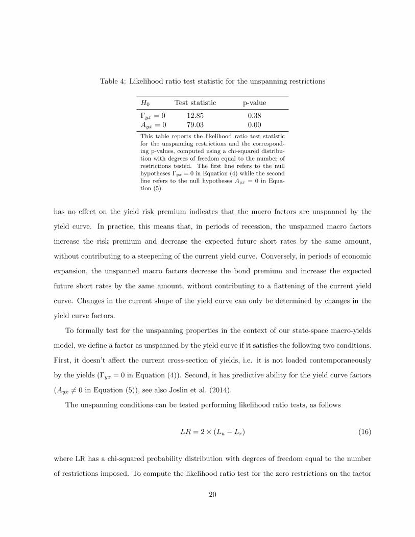
Table 4: Likelihood ratio test statistic for the unspanning restrictions

H0 Test statistic p-value

Γyx = 0 12.85 0.38Ayx = 0 79.03 0.00

This table reports the likelihood ratio test statisticfor the unspanning restrictions and the correspond-ing p-values, computed using a chi-squared distribu-tion with degrees of freedom equal to the number ofrestrictions tested. The first line refers to the nullhypotheses Γyx = 0 in Equation (4) while the secondline refers to the null hypotheses Ayx = 0 in Equa-tion (5).

has no effect on the yield risk premium indicates that the macro factors are unspanned by the

yield curve. In practice, this means that, in periods of recession, the unspanned macro factors

increase the risk premium and decrease the expected future short rates by the same amount,

without contributing to a steepening of the current yield curve. Conversely, in periods of economic

expansion, the unspanned macro factors decrease the bond premium and increase the expected

future short rates by the same amount, without contributing to a flattening of the current yield

curve. Changes in the current shape of the yield curve can only be determined by changes in the

yield curve factors.

To formally test for the unspanning properties in the context of our state-space macro-yields

model, we define a factor as unspanned by the yield curve if it satisfies the following two conditions.

First, it doesn’t affect the current cross-section of yields, i.e. it is not loaded contemporaneously

by the yields (Γyx = 0 in Equation (4)). Second, it has predictive ability for the yield curve factors

(Ayx 6= 0 in Equation (5)), see also Joslin et al. (2014).

The unspanning conditions can be tested performing likelihood ratio tests, as follows

LR = 2× (Lu − Lr) (16)

where LR has a chi-squared probability distribution with degrees of freedom equal to the number

of restrictions imposed. To compute the likelihood ratio test for the zero restrictions on the factor

20

loadings, Lu denotes the loglikelihood of an unrestricted macro-yield model that does not impose

the restriction Γyx = 0 and Lr is the loglikelihood of our macro-yields model. The test statistic

in Table 4 shows that we cannot reject the null hypothesis of factor loadings of the yields on the

macro factors equal to zero. This implies that, indeed, the macro factors do not affect the current

shape of the yield curve.12

To test the predictive ability of the macro factors obtained from macro-yields model in Equa-

tions (4)–(6) for the yield factors, and therefore the yield curve of interest rates, we perform the

likelihood ratio test statistics in Equation (16), where, in this case, Lu is the loglikelihood of our

macro-yield model and Lr is the restricted loglikelihood obtained imposing Ayx = 0 in Equation

(5). Results in Table 4 show that we can reject the null hypothesis of no Granger causality from

the macro factors to the yield curve factors.

The result of the test shows that the macroeconomic factors identified by the macro-yields

model do not explain the cross-section of yields but have predictive ability for the future evolution

of the yield curve. As a consequence, they satisfy both conditions for being truly unspanned

macroeconomic factors.13

5 Out-of-sample forecast

To evaluate the predictive ability of the macro-yields model, we generate out-of-sample iterative

forecasts of the factors, as follows

Et(F∗t+h) ≡ F ∗t+h|t = (A∗|t)

hF ∗t|t,

12This result is due to the fact that almost all the bond yields variation is explained by the Nelson and Siegelfactors. The same result may not hold when the yield factors provide a poorer fit of the yields, as in Joslin, Le andSingleton (2013).

13Moreover, looking at the coefficients and their relative standard errors, available upon request, we can infer thatthe first unspanned factor, proxied by economic growth, Granger causes the slope and the curvature, while the secondunspanned factor, proxied by the real interest rate, Granger causes the level.

21

where h denotes the forecast horizon and A∗|t is estimated using the information available till time

t.14 We then compute out-of-sample forecasts of the yields given the projected factors, in this way

Et(zt+h) ≡ zt+h|t = Γ∗|tF∗t+h|t,

where Γ∗|t is estimated using data up to time t.

Collecting the excess returns for bonds with maturities from two to five years in the vector rxt,

we compute the out-of-sample predictions of excess bond returns as follows

Et(rxt+12) ≡ rxt+12|t = Π1yt+12|t + Π2yt = Π1(Γ∗|tF∗t+12|t) + Π2yt, (17)

where Π1 =

[D[−1:−K] 0[K×1]

], Π2 =

[−1[K×1] D[2:K+1]

], D[−1:−K] denotes a diagonal

matrix with elements −1,−2, . . . ,−K in the diagonal and K + 1 denotes the total number of

maturities. Notice that Equation (17) implies that the forecast errors made in forecasting the

excess returns are proportional to the ones made in forecasting the yields, i.e. rxt+12|t − rxt+12 =

Π1(yt+12|t − yt+12), see Carriero, Kapetanios and Marcellino (2012).

We forecast yields and excess returns recursively using data from January 1970 and evaluating

the forecast performances on the sample from January 1990 to December 2008.

5.1 Yields

To evaluate the prediction accuracy of the macro yields model for out-of-sample forecasts of yields,

we use the Mean Squared Forecast Error (MSFE), i.e. the average squared error in the evaluation

period for the h-months ahead forecast of the yield (or excess return) with maturity τ

MSFEt1t0(τ, h,M) =1

t1 − t0 + 1

t1∑t=t0

(y(τ)t+h|t(M)− y(τ)t+h

)2, (18)

14See Appendix A for the definitions of F ∗t , Γ∗ and A∗.

22

Table 5: Out-of-sample performance for yields

Macro-Yields

Maturity 3m 1y 2y 3y 4y 5y

h=1 1.17 1.05 1.06 1.00 1.05 1.14h=3 0.79* 0.93 0.99 0.96 0.99 1.02h=6 0.78** 0.89 0.94 0.93 0.93 0.94h=12 0.69** 0.74** 0.79** 0.80*** 0.80*** 0.80***h=24 0.62*** 0.66*** 0.74** 0.82** 0.88* 0.97

Only-Yields

Maturity 3m 1y 2y 3y 4y 5y

h=1 0.93 1.09 1.17 1.11 1.07 1.11h=3 0.96 1.13 1.20 1.14 1.10 1.13h=6 0.99 1.18 1.25 1.21 1.15 1.16h=12 1.04 1.16 1.26 1.27 1.25 1.26h=24 1.06 1.12 1.27 1.39 1.49 1.62

This table reports the relative MSFE of the macro-yields model and the only-yieldsmodel over the MSFE of the random walk for multi-step predictions of the yields.The first column reports the forecast horizon h. The sample starts on January 1970and the evaluation period is January 1990 to December 2008. *, ** and *** denotesignificant outperformance at 10%, 5% and 1% level with respect to the random walkaccording to the White (2000) reality check test with 1,000 bootstrap replicationsusing an average block size of 12 observations.

where t0 and t1 denote, respectively, the start and the end of the evaluation period, y(τ)t+h is the

realized yield with maturity τ at time t+ h and y(τ)t+h|t(M) is the h-step ahead forecast of the yield

with maturity τ from model M using the information available up to t.

Forecast results for yields are usually expressed as relative performance with respect to the

random walk, which is a naıve benchmark for yield curve forecasting very difficult to outperform,

given the high persistency of the yields. The random walk h-steps ahead prediction at time t of

the yield with maturity τ is

Et(y(τ)t+h) ≡ y(τ)t+h|t = y

(τ)t ,

where the optimal predictor does not change regardless of the forecast horizon. To measure the

relative performance of the macro-yields model with respect to the random walk, we use the relative

23

Figure 4: 12-months ahead smoothed squared forecast errors for yields

95 97 00 02 05 070

0.5

1

1.5

2

2.5

3

3.5 Maturity 3 months

MY RW

95 97 00 02 05 070

0.5

1

1.5

2

2.5

3

3.5 Maturity 3 months

OY RW

95 97 00 02 05 070

0.5

1

1.5

2

2.5

Maturity 36 months

MY RW

95 97 00 02 05 070

0.5

1

1.5

2

2.5

Maturity 36 months

OY RW

95 97 00 02 05 070

0.5

1

1.5

2

Maturity 60 months

MY RW

95 97 00 02 05 070

0.5

1

1.5

2

Maturity 60 months

OY RW

This figure displays the 5-years rolling 12-months ahead squared forecast error for the yields with 3, 36 and 60

months to maturity. The blue continuous line refers to the 5-years rolling squared forecast error of the macro-yields

MY model (left plots) and of the only-yields OY model (right plots). The dashed red line refers to 5-years rolling

squared forecast error of the random walk. The dates on the horizontal axis refer to the end of the rolling window

period. The grey-shaded areas indicate the recessions as defined by the NBER.

24

MSFE computed as

rMSFEt1t0(τ, h,M) =MSFEt1t0(τ, h,M)

MSFEt1t0(τ, h,RW ).

Table 5 reports the rMSFE with respect to the random walk for the macro-yields model the

only-yields model. Results in Table 5 show that the macro-yields model outperforms the only-yields

model for all but 1-month horizon. Moreover, the macro-yields model outperforms the random

walk at 3-, 6-, 12- and 24-month ahead for all the maturities, with significant a out-performance,

according to the White (2000) reality check test, for the 12- and 24-month ahead forecasts.15 This

evidence is corroborated by Figure 4, which reports the 12-month ahead smoothed squared forecast

errors of the macro-yields, the only-yields and the random walk models for yields with 3-, 36- and

60-month to maturity. The figure highlights how the macro-yields model systematically outperforms

the random walk especially in the last part of the evaluation sample for the short maturities, and in

the first part of the sample for long maturities. The only-yield model, instead, performs as well as

the random walk in the first part of the evaluation sample. However, its performance deteriorates

in the last part of the evaluation sample, significantly underperforming the random walk. These

results indicate that the unspanned macroeconomic factors, while not important for explaining the

contemporaneous variation of the yields curve, contain useful information to predict the future

values of the yield curve factors and, thus, the future evolution of the yield curve.

5.2 Excess bond returns

Out-of-sample forecast results for excess bond returns are reported in Table 6, which contains the

relative MSFE of the macro-yields model with respect to the constant excess return benchmark,

where one-year holding period excess returns are unforecastable at one year horizon, as in the ex-

pectation hypothesis. We use the expectation hypothesis since, because of its simplicity, represents

a benchmark of unpredictability. The macro-yields model outperforms the constant excess return

benchmark for all maturities and the outperformance is significant for all maturities according to

the White (2000) reality check test.

15For more details about the reality check test see Appendix C.

25

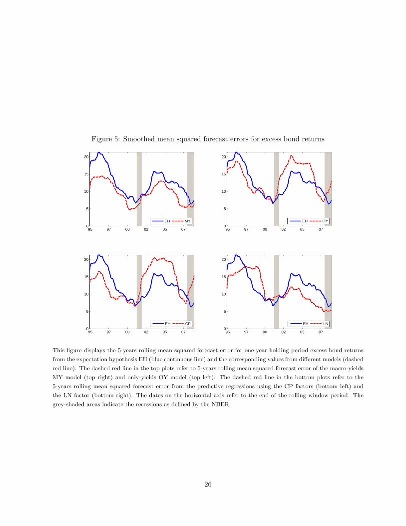
Figure 5: Smoothed mean squared forecast errors for excess bond returns

95 97 00 02 05 070

5

10

15

20

EH MY

95 97 00 02 05 070

5

10

15

20

EH OY

95 97 00 02 05 070

5

10

15

20

EH CP

95 97 00 02 05 070

5

10

15

20

EH LN

This figure displays the 5-years rolling mean squared forecast error for one-year holding period excess bond returns

from the expectation hypothesis EH (blue continuous line) and the corresponding values from different models (dashed

red line). The dashed red line in the top plots refer to 5-years rolling mean squared forecast error of the macro-yields

MY model (top right) and only-yields OY model (top left). The dashed red line in the bottom plots refer to the

5-years rolling mean squared forecast error from the predictive regressions using the CP factors (bottom left) and

the LN factor (bottom right). The dates on the horizontal axis refer to the end of the rolling window period. The

grey-shaded areas indicate the recessions as defined by the NBER.

26

Table 6: Out-of-sample predictive performance for excess returns

Maturity MY OY CP LN LN+CP

2y 0.76** 1.20 1.17 0.80 0.803y 0.75** 1.20 1.21 0.79 0.834y 0.74** 1.18 1.21 0.78 0.835y 0.75** 1.18 1.18 0.81 0.83

This table reports the relative MSFE of the macro-yields model (MY ), the only-yields model (OY ), theCochrane and Piazzesi (2005) factor (CP ), the Ludvig-son and Ng (2009) (LN) factor, the Cochrane and Pi-azzesi (2005) and the Ludvigson and Ng (2009) factorscombined (LN+CP ) with respect to the expectation hy-pothesis for excess returns. The sample starts on January1970 and the evaluation period is January 1990 to De-cember 2008. * and ** denote significant outperformanceat 10% and 5% level with respect to the expectation hy-pothesis according the White (2000) reality check testwith 1,000 bootstrap replications using an average blocksize of 12 observations.

Table 6 also reports the out-of-sample relative MSFEs of the excess bond returns forecasts

using the CP factor, the LN factor, and the CP and LN factors combined obtained from the

predictive regressions in equation (14). The worst performing models are the ones that do not use

macroeconomic variable, i.e., the only-yield model and the CP factors. In line with the predictive

regressions of excess bond returns and with the 12-month ahead out-of-sample forecast performance

of the macro-yields model for the yields, results in Table 6 show that the macro-yields model is

the best performing model for the prediction of the 1-year excess bond returns for all maturities

followed by the combination of the CP and LN factors. However, although the unspanned model

significantly outperforms the naıve benchmark while the CP+LN does not, we cannot reject the

hypothesis that the forecasts of these two models are statistically equally accurate.

To further understand the performance of the macro-yields model to predict 1-year holding

period excess bond returns, Figure 5 plots the 5-year rolling mean squared forecast error of the

macro-yields model, the only-yields model, the CP and LN factors along with the 5-year rolling

mean squared forecast error under the expectation hypothesis (EH). The figure shows that the

performance of the only-yield model and the CP factors are similar: both models outperform the

27

expectation hypothesis in the first part of the evaluation sample but display large forecast errors in

the second part. Also the performance of the macro-yields model and the LN factors are similar,

they both provide more accurate predictions than the expectation hypothesis, in particular in the

last part of the evaluation period. The better accuracy of the macro-yields model relative to LN

factors in Table 6 is coming mainly from the first half of the evaluation sample, up to the end of

the 90’s. In that period the macro-yields model significantly outperforms the EH, while the LN

factors do not. Afterward both the macro-yields and the LN models outperform significantly the

EH and are equally accurate.

However, the figure shows that the macro-yields model, apart from being the best performing

model on average, as shown in Table 6, it is the best performing model for the whole evaluation

period. This is a clear evidence that the unspanned macroeconomic factors identified by the pro-

posed macro-yields model have predictive ability for the yield curve factors and, thus, for excess

bond returns.

6 Conclusions

In this paper we analyze the predictive content of macroeconomic information for the yield curve of

interest rates and excess bond returns in the United States. We find that two macroeconomic factors

characterizing economic growth and real interest are unspanned by the cross-section of government

bond yields and have significant predictive power for the bond yields and excess returns.

In future research, we plan to extend our empirical specification to allow for the zero lower

bound of interest rates, non-synchronicity of macroeconomic data releases and mixed frequencies.

The macro-yields model presented in this paper cannot be estimated on a sample that includes

the great recession, as it does not honor the zero lower bound for the interest rates. However, our

model model can be easily extended to deal with this issue by anchoring the shorter end of the

yield curve using market expectation, along the lines of Altavilla, Giacomini and Ragusa (2014).

Data revisions and jagged edges due to the non-synchronicity of macroeconomic data releases

28

are important characteristics to be taken into account when extracting macroeconomic information,

see Giannone, Reichlin and Small (2008). In addition, bond yields are available at higher frequencies

than macroeconomic variables. These features can be easily incorporated into our empirical model

along the line described in Banbura et al. (2012).

29

A Estimation procedure

We can rewrite the macro-yields model in equations (4)–(6) in compact form as

zt = a+ ΓFt + vt, (19)

Ft = µ+AFt−1 + ut, ut ∼ N(0, Q) (20)

vt = Bvt−1 + ξt, ξt ∼ N(0, R) (21)

where zt =

ytxt

, Ft =

F ytF xt

, a =

0

ax

, Γ =

Γyy Γyx

Γxy Γxx

, A =

Ayy Ayx

Axy Axx

, Q =

Qyy Qyx

Qxy Qxx

,

µ =

µyµx

and Γyy = ΓNS is the matrix whose rows correspond to the smooth patterns proposed

by Nelson and Siegel (1987) and shown in equation (2). In addition Γyx = 0, as the macroeconomic

factors F xt are unspanned by the cross-section of yields Γyx = 0. We also estimate the only-yields

model using the same procedure, as it implies the following restrictions in (19)–(20): zt = yt, Ft =

F yt , a = 0, Γ = ΓNS , µ = µy.

The macro-yields model in (19)–(20) can be put in a state-space form augmenting the states Ft

with the idiosyncratic components vt and a constant ct as follows

zt = Γ∗F ∗t + v∗t , v∗t ∼ N(0, R∗)

F ∗t = A∗F ∗t−1 + u∗t , u∗t ∼ N(0, Q∗)

where Γ∗ =

[Γ a IN

], F ∗t =

Ft

ct

vt

, A∗ =

A µ . . . 0

... . ..

1...

0 . . . . . . B

, u∗t =

ut

νt

ξt

, Q∗ =

Q . . . 0

... ε...

0 . . . R

and R = εIn, with ε a very small fixed coefficient. In this state-space form, ct an additional state

variable restricted to one at every time t.

30

The restrictions on the factor loadings Γ∗ and on the transition matrix A∗ can be written as

H1 vec(Γ∗) = q1, H2 vec(A∗) = q2,

where H1 and H2 are selection matrices, and q1 and q2 contain the restrictions.

We assume that F ∗1 ∼ N(π1, V1), and define y = [y1, . . . , yT ] and F ∗ = [F ∗1 , . . . , F∗T ]. Then

denoting the parameters by θ = {Γ∗, A∗, Q∗, π1, V1}, we can write the joint loglikelihood of zt and

Ft, for t = 1, . . . , T , as

L(z, F ∗; θ) = −T∑t=1

(1

2[zt − Γ∗F ∗t ]′ (R∗)−1 [zt − Γ∗F ∗t ]

)+

−T2

log |R∗| −T∑t=2

(1

2[F ∗t −A∗F ∗t−1]′(Q∗)−1[F ∗t −A∗F ∗t−1]

)+

−T − 1

2log |Q∗|+ 1

2[F ∗1 − π1]′V −11 [F ∗1 − π1] +

−1

2log |V1| −

T (p+ k)

2log 2π + λ′1 (H1 vec(Γ∗)− q1) + λ′2 (H2 vec(A∗)− q2)

where λ1 contains the lagrangian multipliers associate with the constraints on the factor loadings

Γ∗ and λ2 contains the lagrangian multipliers associated with the constraints on the transition

matrix A∗.

The computation of the Maximum Likelihood estimates is performed using the EM algorithm.

Broadly speaking, the algorithm consists in a sequence of simple steps, each of which uses the

Kalman smoother to extract the common factors for a given set of parameters and closed form

solutions to estimate the parameters given the factors. In practice, we use the restricted version of

the EM algorithm, the Expectation Restricted Maximization, since we need to impose the smooth

pattern on the factor loadings of the yields on the NS factors. The ERM algorithm alternates

Kalman filter extraction of the factors to the restricted maximization of the likelihood. At the j-th

iteration the ERM algorithm performs two steps:

1. In the Expectation-step, we compute the expected log-likelihood conditional on the data and

31

the estimates from the previous iteration, i.e.

L(θ) = E[L(z, F ∗; θ(j−1))|z]

which depends on three expectations

F ∗t ≡ E[F ∗t ; θ(j−1)|z]

Pt ≡ E[F ∗t (F ∗t )′; θ(j−1)|z]

Pt,t−1 ≡ E[F ∗t (F ∗t−1)′; θ(j−1)|z]

These expectations can be computed, for given parameters of the model, using the Kalman

filter.

2. In the Restricted Maximization-step, we update the parameters maximizing the expected

log-likelihood with respect to θ:

θ(j) = arg maxθL(θ)

This can be implemented taking the corresponding partial derivative of the expected log

likelihood, setting to zero, and solving.

The procedure outlined above can be extended to estimate also the decay parameter λ controlling

for the shape of the loadings of the yields on the slope and curvature factors. Since the factor

loadings are a non-linear function λ, an additional step consisting in the numerical maximization

of the conditional likelihood with respect to λ is required. The procedure is know as Expectation

Conditional Restricted Maximization (ECRM) algorithm.

32

B Data

Table 7: Macroeconomic variables

Series N. Mnemonic Description Transformation

1 AHE Average Hourly Earnings: Total Private 12 CPI Consumer Price Index: All Items 13 INC Real Disposable Personal Income 14 FFR Effective Federal Funds Rate 05 HSal House Sales - New One Family Houses 16 IP Industrial Production Index 17 M1 M1 Money Stock 18 Manf ISM Manufacturing: PMI Composite Index (NAPM) 09 Paym All Employees: Total nonfarm 110 PCE Personal Consumption Expenditures 111 PPIc Producer Price Index: Crude Materials 112 PPIf Producer Price Index: Finished Goods 113 CU Capacity Utilization: Total Industry 014 Unem Civilian Unemployment Rate 0

This table lists the 14 macro variables used to estimate the macro-yields. Most series have been transformedprior to the estimation, as reported in the last column of the table. The transformation codes are: 0 = notransformation and 1 = annual growth rate.

C Reality check test

To compare the out-of-sample predictive ability of a model with respect to the benchmark, we use

the reality check test of White (2000), as we compare only non-nested models.

If we denote by et(b) the forecast errors of the benchmark and by et(M) the forecast errors of

the model under consideration. Then we can define the null hypothesis of no predictive superiority

over the benchmark as

H0 : f = E(ft) ≡ E(et(b)2 − et(M)2) ≤ 0 (22)

The test is then based on the statistic

f =1

t1 − t0

t1∑t=t0

ft (23)

33

where t0 and t1 denote, respectively, the start and the end of the evaluation period, and hats denote

estimated statistics.

To approximate the asymptotic distribution of the test statistic, we use block-bootstrap as

follows:

1. We generate bootstrapped forecast errors e∗t (b) and e∗t (M) using the stationary block-bootstrap

of Politis and Romano (1994) with average block size of 12. This procedure is analogous to

the moving blocks bootstrap, but, instead of using blocks of fixed length uses blocks of ran-

dom length, distributed according to the geometric distribution with mean block length 12.

Also to give the same probability of resampling to all observations, we use a circular scheme.

2. Construct the bootstrapped test statistic as

f∗

=1

t1 − t0

t1∑t=t0

(e∗t (b)2 − e∗t (M)2)

3. Repeat steps 1 and 2 for 1,000 times to obtain an estimate of the distribution of the test

statistic f∗

= [f∗(1), . . . , f

∗(1,000)].

4. Compare V = (t1 − t0)1/2f with the quantiles of V ∗ = (t1 − t0)1/2(f∗ − f) to obtain the

p-value.

34

References

Altavilla, Carlo, Raffaella Giacomini, and Giuseppe Ragusa (2014) ‘Anchoring the yield curve usingsurvey expectations.’ ECB Working Paper

Ang, Andrew, and Monika Piazzesi (2003) ‘A No-Arbitrage Vector Autoregression of Term Struc-ture Dynamics with Macroeconomic and Latent Variables.’ Journal of Monetary Economics50(4), 745–787

Ang, Andrew, Monika Piazzesi, and Min Wei (2006) ‘What Does the Yield Curve Tell us aboutGDP Growth.’ Journal of Econometrics 131, 359–403

Bai, Jushan, and Serena Ng (2002) ‘Determining the Number of Factors in Approximate FactorModels.’ Econometrica 70(1), 191–221

Banbura, Marta, Domenico Giannone, Michele Modugno, and Lucrezia Reichlin (2012) ‘Now-casting and the real-time data flow.’ Handbook of Economic Forecasting, G. Elliott andA. Timmermann, eds., Volume 2, Elsevier-North Holland

Bianchi, Francesco, Haroon Mumtaz, and Paolo Surico (2009) ‘The great moderation of the termstructure of uk interest rates.’ Journal of Monetary Economics 56(6), 856–871

BIS (2005) Zero-Coupon Yield Curves: Technical Documentation (Bank for International Settle-ments, Basle)

Campbell, John Y, and Robert J Shiller (1991) ‘Yield spreads and interest rate movements: Abird’s eye view.’ The Review of Economic Studies 58(3), 495–514

Carriero, Andrea, George Kapetanios, and Massimiliano Marcellino (2012) ‘Forecasting govern-ment bond yields with large bayesian vector autoregressions.’ Journal of Banking & Finance36(7), 2026–2047

Cochrane, John H, and Monika Piazzesi (2005) ‘Bond risk premia.’ American Economic Review95(1), 138–160

Cooper, Ilan, and Richard Priestley (2009) ‘Time-varying risk premiums and the output gap.’Review of Financial Studies 22(7), 2801–2833

Coroneo, Laura, Ken Nyholm, and Rositsa Vidova-Koleva (2011) ‘How arbitrage-free is the Nelson–Siegel model?’ Journal of Empirical Finance 18(3), 393–407

De Pooter, Michiel, Francesco Ravazzolo, and Dick JC Van Dijk (2007) ‘Predicting the Term Struc-ture of Interest Rates: Incorporating Parameter Uncertainty and Macroeconomic Information.’Tinbergen Institute Discussion Papers

Dewachter, Hans, and Marco Lyrio (2006) ‘Macro factors and the term structure of interest rates.’Journal of Money, Credit and Banking 38(1), 119–140

35

Diebold, Francis X, and Canlin Li (2006) ‘Forecasting the term structure of government bondyields.’ Journal of Econometrics 130, 337–364

Diebold, Francis X, and Glenn D Rudebusch (2013) Yield Curve Modeling and Forecasting: TheDynamic Nelson-Siegel Approach, vol. 1 of Economics Books (Princeton University Press)

Diebold, Francis X, Glenn D Rudebusch, and S Boragan Aruoba (2006) ‘The macroeconomy andthe yield curve: A dynamic latent factor approach.’ Journal of Econometrics 131, 309–338

Doz, Catherine, Domenico Giannone, and Lucrezia Reichlin (2011) ‘A two-step estimator forlarge approximate dynamic factor models based on kalman filtering.’ Journal of Econometrics164(1), 188–205

(2012) ‘A quasimaximum likelihood approach for large, approximate dynamic factor models.’The Review of Economics and Statistics 94(4), 1014–1024

Duffee, Gregory R (2011a) ‘Forecasting with the term structure: The role of no-arbitrage re-strictions.’ Technical Report, Working papers//the Johns Hopkins University, Department ofEconomics

(2011b) ‘Information in (and not in) the term structure.’ Review of Financial Studies24(9), 2895–2934

ECB (2008) The new Euro Area yield curves February Monthly Bulletin (European Central Bank,Franfurt)

Fama, Eugene F, and Robert R Bliss (1987) ‘The Information in Long-Maturity Forward Rates.’The American Economic Review 77(4), 680–692

Favero, Carlo A, Linlin Niu, and Luca Sala (2012) ‘Term structure forecasting: No-arbitrage re-strictions versus large information set.’ Journal of Forecasting 31(2), 124–156

Giannone, Domenico, Lucrezia Reichlin, and David Small (2008) ‘Nowcasting: The real-time infor-mational content of macroeconomic data.’ Journal of Monetary Economics 55(4), 665–676

Giannone, Domenico, Lucrezia Reichlin, and Luca Sala (2005) ‘Monetary policy in real time.’In ‘NBER Macroeconomics Annual 2004, Volume 19’ NBER Chapters (National Bureau ofEconomic Research, Inc) pp. 161–224

Gurkaynak, Refet S, Brian Sack, and Jonathan H Wright (2007) ‘The us treasury yield curve: 1961to the present.’ Journal of Monetary Economics 54(8), 2291–2304

Joslin, Scott, Anh Le, and Kenneth J Singleton (2013) ‘Why gaussian macro-finance term structuremodels are (nearly) unconstrained factor-vars.’ Journal of Financial Economics 109(3), 604–622

Joslin, Scott, Marcel Priebsch, and Kenneth J Singleton (2014) ‘Risk premiums in dynamic termstructure models with unspanned macro risks.’ The Journal of Finance 69(3), 1197–1233

36

Litterman, Robert B, and Jose Scheinkman (1991) ‘Common factors affecting bond returns.’ Jour-nal of Fixed Income 47, 129–1282

Ludvigson, Sydney C, and Serena Ng (2009) ‘Macro factors in bond risk premia.’ Review of Finan-cial Studies 22(12), 5027

Monch, Emanuel (2008) ‘Forecasting the yield curve in a data-rich environment: A no-arbitragefactor-augmented var approach.’ Journal of Econometrics 146(1), 26–43

(2012) ‘Term structure surprises: The predictive content of curvature, level, and slope.’ Journalof Applied Econometrics 27(4), 574–602

Nelson, Charles R, and Andrew F Siegel (1987) ‘Parsimonious modeling of yield curves.’ Journalof Business 60, 473–89

Politis, Dimitris N, and Joseph P Romano (1994) ‘The Stationary Bootstrap.’ Journal of the Amer-ican Statistical Association

Rudebusch, Glenn D, and Tao Wu (2008) ‘A Macro-Finance Model of the Term Structure, MonetaryPolicy and the Economy.’ Economic Journal 118(530), 906–926

Sargent, Thomas J, Christopher A Sims et al. (1977) ‘Business cycle modeling without pretending tohave too much a priori economic theory.’ New Methods in Business Research, Federal ReserveBank of Minneapolis, Minneapolis

Taylor, John B (1993) ‘Discretion versus policy rules in practice.’ Carnegie-Rochester ConferenceSeries on Public Policy 39(1), 195–214

Thornton, Daniel L, and Giorgio Valente (2012) ‘Out-of-sample predictions of bond excess returnsand forward rates: An asset allocation perspective.’ Review of Financial Studies 25(10), 3141–3168

Watson, Mark W (2005) ‘Comment on monetary policy in real time, by domenico giannone, lucreziareichlin, and luca sala.’ In ‘NBER Macroeconomics Annual 2004, Volume 19’ NBER Chapters(National Bureau of Economic Research, Inc) pp. 216–221.

White, Halbert (2000) ‘A reality check for data snooping.’ Econometrica 68(5), 1097–1126

Wright, Jonathan H (2011) ‘Term premia and inflation uncertainty: Empirical evidence from aninternational panel dataset.’ The American Economic Review 101(4), 1514–1534

37