UNIVERSITY OF NOVA GORICASCHOOL OF APPLIED SCIENCES

THE PEROXY LINKAGE IN AMORPHOUS SILICA:ELECTRONIC AND OPTICAL PROPERTIES FROM

AB-INITIO MODELING

MASTER THESIS

Blaz Winkler

Mentor: Doc. Dr. Layla Martin-Samos

Nova Gorica, 2014

UNIVERZA V NOVI GORICIFAKULTETA ZA APLIKATIVNO NARAVOSLOVJE

PEROKSIDNA VEZ V AMORFNEM SILICIJU:ELEKTRONSKE IN OPTICNE LASTNOSTI IZ

AB-INITIO MODELIRANJA

MAGISTERSKO DELO

Blaz Winkler

Mentor: Doc. Dr. Layla Martin-Samos

Nova Gorica, 2014

Acknowledgement

I would like to express my deepest gratitude to my mentor, doc. dr. Layla Martin-

Samos for all the help provided in the making of the thesis. Many aspects of this work

would not be possible without all the meaningful lectures, thorough guidance and your

endless patience. Thank you!

This work was performed using the GENCI-CCRT High Performance Computing re-

sources (DARI Grant number 2014096137).

I would also like to thank all of the staff from University of Nova Gorica for all the

assistance throughout the study. Special mention to Ana for never giving up. Last but

not least I would like to thank my family for their unconditional support, especially

grandmother Helena.

i

Abstract

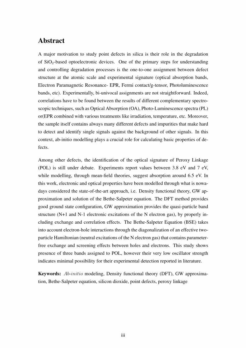
A major motivation to study point defects in silica is their role in the degradation

of SiO2-based optoelectronic devices. One of the primary steps for understanding

and controlling degradation processes is the one-to-one assignment between defect

structure at the atomic scale and experimental signature (optical absorption bands,

Electron Paramagnetic Resonance- EPR, Fermi contact/g-tensor, Photoluminescence

bands, etc). Experimentally, bi-univocal assignments are not straightforward. Indeed,

correlations have to be found between the results of different complementary spectro-

scopic techniques, such as Optical Absorption (OA), Photo-Luminescence spectra (PL)

or(EPR combined with various treatments like irradiation, temperature, etc. Moreover,

the sample itself contains always many different defects and impurities that make hard

to detect and identify single signals against the background of other signals. In this

context, ab-initio modelling plays a crucial role for calculating basic properties of de-

fects.

Among other defects, the identification of the optical signature of Peroxy Linkage

(POL) is still under debate. Experiments report values between 3.8 eV and 7 eV,

while modelling, through mean-field theories, suggest absorption around 6.5 eV. In

this work, electronic and optical properties have been modelled through what is nowa-

days considered the state-of-the-art approach, i.e. Density functional theory, GW ap-

proximation and solution of the Bethe-Salpeter equation. The DFT method provides

good ground state configuration, GW approximation provides the quasi-particle band

structure (N+1 and N-1 electronic excitations of the N electron gas), by properly in-

cluding exchange and correlation effects. The Bethe-Salpeter Equation (BSE) takes

into account electron-hole interactions through the diagonalization of an effective two-

particle Hamiltonian (neutral excitations of the N electron gas) that contains parameter-

free exchange and screening effects between holes and electrons. This study shows

presence of three bands assigned to POL, however their very low oscillator strength

indicates minimal possibility for their experimental detection reported in literature.

Keywords: Ab-initio modeling, Density functional theory (DFT), GW approxima-

tion, Bethe-Salpeter equation, silicon dioxide, point defects, peroxy linkage

iii

Povzetek

Studija tockastih deformacij silicija je zanimiva zaradi njihove vloge pri degradaciji

opticno-elektricnih naprav zgrajenih iz silicijevega dioksida - SiO2. Eden izmed prvih

korakov pri razumevanju in nadzoru degradacije je povezovanje med defekti na atom-

ski skali in eksperimentalnimi rezultati (opticni absorpcijski pasovi, elektronska para-

magnetna resonanca, fotolumiscencni pasovi,... ), kar pa ni vedno enostavno razvidno.

Posledicno moramo poiskati korelacije med rezultati razlicnih komplementarnih spek-

troskopskih tehnik kot so: opticna absorpcijska spektroskopija(OA), fotolumiscencna

spektroskopija (PL) ali elektronska paramagnetna resonanca (EPR) v kombinaciji z

razlicnimi postopki npr. temperatura, obsevanje,... Poleg tega vzorec vedno vsebuje

razlicne defekte in necistoce zaradi katerih tezko locimo posamezne signale od ostalih

signalov oz. ozadja. V tem kontekstu ima ab-initio modeliranje osrednjo vlogo pri

izracunu osnovnih lastnosti defektov.

Med drugimi defekti je identifikacija opticne sledi peroksidne vezi (PerOxyLinkage -

POL) se vedno predmet studij. Eksperimentalna porocila opisujejo energijo absorpcije

med 3.8eV in 7eV medtem ko rezultati modeliranja nakazujejo vrednost okrog 6.5 eV.

V tem delu so predstavljene elektronske in opticne lastnosti modelirane z najnapre-

dnejsimi metodami: Gostotna funkcijska teorija (”Density Functional Theory- DFT),

GW priblizkom in resitvami Bethe-Salpeterjeve enacbe. DFT metoda sluzi izracunu

osnovnega stanja, GW priblizek opisuje pasovno strukturo kvazi-delcev (N+1 in N-

1 elektronskih vzbuditev N-elektronskega plina) z natancnim obravnavanjem izme-

njevalnih ter korelacijskih efektov. Bethe-Salpeterjeva enacba (BSE) opisuje interak-

cijo elektron-vrzel z diagonalizacijo Hamiltonovega operatorja dveh delcev (nevtralno

vzbujanje N-elektronskega plina) kateri vsebuje izmenjavo prek prostih parametrov in

ucinkov sencenja med vrzelmi in elektroni. Ta studija pokaze navzocnost treh absorp-

cijskih pasov izhajajocih iz peroksidnega defekta. Zelo nizke verjetnosti opticnega

vzbujanja nakazujejo malo moznosti, da bi opisane prehode lahko zaznali z eksperi-

mentalnimi metodami opisanimi v literaturi.

Kljucne besede: Ab-initio modeliranje, gostotna funkcijska teorija (DFT), GW pri-

blizek, Bethe-Salpeterjeva enacba, silicijev dioksid, tockaste deformacije , peroksidna

vez

v

Contents

1 Introduction 1

2 Theoretical framework 32.1 Introduction . . . . . . . . . . . . . . . . . . . . . . . . . . . . . . . 3

2.2 Basics of Density Functional Theory . . . . . . . . . . . . . . . . . . 5

2.3 Basics of GW . . . . . . . . . . . . . . . . . . . . . . . . . . . . . . 7

2.4 DFT in practice . . . . . . . . . . . . . . . . . . . . . . . . . . . . . 10

2.4.1 Approximation to exchange functional . . . . . . . . . . . . . 10

2.4.2 Plane wave expansion and Bloch theorem . . . . . . . . . . . 10

2.4.3 The pseudo potential approximation . . . . . . . . . . . . . . 11

2.4.4 Ewald summation . . . . . . . . . . . . . . . . . . . . . . . . 13

2.4.5 Born-Oppenheimer approximation . . . . . . . . . . . . . . . 14

2.5 GW in practice . . . . . . . . . . . . . . . . . . . . . . . . . . . . . 15

2.5.1 The plasmon-pole model . . . . . . . . . . . . . . . . . . . . 16

2.5.2 Perturbative GW, GW@DFT . . . . . . . . . . . . . . . . . . 17

2.6 Bethe-Salpeter equation . . . . . . . . . . . . . . . . . . . . . . . . . 17

3 Peroxy linkage defect in silica 203.1 H2O2 . . . . . . . . . . . . . . . . . . . . . . . . . . . . . . . . . . 22

3.2 Silica . . . . . . . . . . . . . . . . . . . . . . . . . . . . . . . . . . 25

4 Conclusion 30

vii

List of Figures

2.1 Left: Electrons in ground state, Middle: ”Photo emission” - Electron

is removed from crystal leaving a hole ie. N-1 particles in the system,

Right: ”Inverse photo emission” - Additional electron is introduced

into system to fill an unoccupied state, producing N+1 particle system 4

2.2 Schematic view of a neutral excitation: formation of an interacting

electron-hole pair . . . . . . . . . . . . . . . . . . . . . . . . . . . . 4

2.3 Procedure for calculation of total energy using conventional matrix di-

agonalization . . . . . . . . . . . . . . . . . . . . . . . . . . . . . . 14

3.1 Left - Unrelaxed H2O2 structure, Right - Relaxed H2O2 structure [19] 22

3.2 Plot of the absorption spectrum with respect to the photon energy. An

artificial broadening of 0.001 eV has been used. . . . . . . . . . . . . 25

3.3 Silica model with lowest formation energy. Silicon atoms are repre-

sented in blue and oxygen in red. Peroxy bridge defect is highlighted 25

3.4 Schematic presentation of electronic structure in POL defect induced

silica . . . . . . . . . . . . . . . . . . . . . . . . . . . . . . . . . . . 26

3.5 Schematic presentation of electronic structure in POL defect induced

silica . . . . . . . . . . . . . . . . . . . . . . . . . . . . . . . . . . . 27

3.6 Absorption spectra of ”pure” silica and defect induced models. Black

arrows are used to indicate POL induced excitons that have very small

oscillator strengths. . . . . . . . . . . . . . . . . . . . . . . . . . . . 29

viii

List of Tables

3.1 Kohn-Sham eigenvalues and square modulus of the corresponding wave-

function. O atoms are in red and H atoms in blue . . . . . . . . . . . 23

3.2 GW corrections for H2O2 molecule . . . . . . . . . . . . . . . . . . . 24

3.3 List of the first four electron-hole excitations with their respective os-

cillator strength . . . . . . . . . . . . . . . . . . . . . . . . . . . . . 24

3.4 Comparison of calculated KS and GW energies . . . . . . . . . . . . 27

3.5 List of first four excitons for the POL in silica model with lowest for-

mation energy . . . . . . . . . . . . . . . . . . . . . . . . . . . . . 28

ix

List of Acronyms

a-SiO2 - Amorphous-SiO2

BCB - Bottom of conduction band

BSE - Bethe Salpeter equation

CI - Configuration interaction

DFT - Density functional theory

EA - Electron affinity

EPR - Electronic paramagnetic resonance

HF - Hartree Fock

HOMO - Highest occupied molecular orbital

HPC - High performance computing

KS - Kohn Sham

LDA - Local density approximation

LUMO - Lowest unoccupied molecular orbital

MOSFET - Metal oxide semiconductor field effect transistor

OA - Optical absorption

PL - Photo luminescence

POL - Peroxy linkage

TDDFT - Time dependant density functional theory

TVB - Top of valence band

VIP - Vertical ionization potential

1. Introduction

Amorphous Silicon dioxide (a-SiO2), commonly referred as silica, is a high dielec-

tric material widely used in many applications such as gate oxide in MOSFET, optical

fibers and lithography. It can be easily manufactured at a relatively low cost. Its huge

band gap (9.6 eV) and huge optical gap (9 eV) together with its dielectric properties

and high thermal stability make silica a unique material, very difficult to replace. In all

the modern applications, it is very important to control defects (and defect precursors)

as they may create defect levels within the band-gap that could reduce the performance

of silica-based devices (electronic losses and optical attenuations). For devices submit-

ted to harsh environments, the knowledge and control of defects becomes even more

crucial, as irradiation induces ionization of pre-existing defects and/or creation of new

defects through knock-on processes, such modifying substantially (and most of the

time irreversibly) the optoelectronic-properties. Is in particular for these kinds of envi-

ronments, that the study of fundamental aspects of silica is getting an increased interest

in the material science community. Indeed, in the field of nuclear technology, optical

fibers based on silica are, at the moment, the sole candidates for communication and

sensing.

Despite 50 years of intensive research and applications, a complete picture of silica

and its defects is still missing. Experimentally a one-to-one assignment between de-

fect signatures and guessed defect atomic structure needs the combination of many

experimental techniques (among others, Electron Paramagnetic Resonance, various

types of Luminescence, optical absorption) that comprise measurements at different

conditions together with hypothesis on the atomic structure and how are defects cre-

ated, how they recombine and how they are annihilated. In the case of silica, as it is an

amorphous material, i.e. disordered, this assignment is even more difficult as defects

may be ”anything”. Indeed, contrary to SiO2 crystalline polymorphs, even the silica

atomic structure, disregarding ”defects”, is unknown. The ideal a-SiO2 is supposed to

be a random network of SiO4 tetrahedral, with an atomic density of 2.2 g/cm. The sole

information about medium range arrangements comes from Raman experiments and

1

modeling that have proven the presence of 3 and 4 tetrahedral rings [9]. In this context,

it is clear that materials modeling may play a fundamental role.

In this thesis we will focus on optoelectronic properties of the PerOxy Linkage (POL).

POL is an intrinsic defect arising from an excess of oxygen, from thermodynamic

equilibrium with O2 gas or from the creation of an oxygen Frenkel pair. The atomic

structure of the defect is a ≡ Si − O − O − Si ≡ bridge. It is of interest, because

in most of the silica applications, silica-based devices are submitted to oxygen partial

pressure.

Under the experimental point of view, optical absorption data on the POL are scarce

and controversial. Imai et al. [17] have attributed a broad absorption bump in the region

of 6.5-7.8 eV to POL, while Nishikava et al. [26] have assigned a weak band at 3.8 eV

in the spectrum of a sample of synthetic silica. On the theoretical side, calculations are

rare and performed with very drastic approximations. The first theoretical estimation

gives a first optically active transition at 8.6 eV [15]. More sophisticated Quantum

Chemistry calculations on very small SiO2 clusters, have given a value of 6.5 eV for

the lowest transition [13]. In this work, we will use state-of-the art first-principles

approaches for modeling the optical signature of POL. Our approach allows for the

parameter-free determination of the optical transitions and optical absorption spectra

taking into account exchange and correlation effects, electron-hole interactions and the

long-range dielectric behavior of the material under study.

In the first chapter of this thesis we will first present the theoretical framework and

then discuss our results on the peroxy bridge.

2

2. Theoretical framework

2.1 Introduction

Modeling optoelectronic properties needs the solution for the ground state of N inter-

acting electrons through Coulomb potential plus the solution of charged and neutral

excitations, see figures 2.1 and 2.2. Being a many body problem, only approximate

solutions are accessible. In the field of quantum mechanical electronic modeling, two

types are commonly used: first principle and semi-empirical methods. The latter uti-

lize certain assumptions based on previous experimental data (empirical modeling,

statistical input and fitting parameters) in order to simplify calculations and speed up

the process. Reliance on empirical parameters can however greatly reduce accuracy

of such approach. Methods based on first principle (often referred as ab initio) indis-

putably provide fundamental picture of the nature and its properties at the price of very

demanding computational cost. [1]

Here we will concentrate on what is nowadays state-of-the-art approach for modeling

opto-electronic properties from first principles, which is based on perturbative GW1 on

top of Density Functional Theory (DFT) calculations.

1While symbols G and W represent certain quantities with physical/mathematical meaning, the

method is never presented with their full name and simply referred as GW approximation

3

Figure 2.1: Left: Electrons in ground state, Middle: ”Photo emission” - Electron is

removed from crystal leaving a hole ie. N-1 particles in the system, Right: ”Inverse

photo emission” - Additional electron is introduced into system to fill an unoccupied

state, producing N+1 particle system

Figure 2.2: Schematic view of a neutral excitation: formation of an interacting

electron-hole pair

4

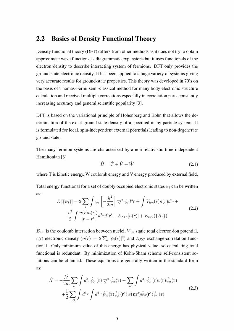
2.2 Basics of Density Functional Theory

Density functional theory (DFT) differs from other methods as it does not try to obtain

approximate wave functions as diagrammatic expansions but it uses functionals of the

electron density to describe interacting system of fermions. DFT only provides the

ground state electronic density. It has been applied to a huge variety of systems giving

very accurate results for ground-state properties. This theory was developed in 70’s on

the basis of Thomas-Fermi semi-classical method for many body electronic structure

calculation and received multiple corrections especially in correlation parts constantly

increasing accuracy and general scientific popularity [3].

DFT is based on the variational principle of Hohenberg and Kohn that allows the de-

termination of the exact ground state density of a specified many-particle system. It

is formulated for local, spin-independent external potentials leading to non-degenerate

ground state.

The many fermion systems are characterized by a non-relativistic time independent

Hamiltonian [3]

H = T + V + W (2.1)

where T is kinetic energy, W coulomb energy and V energy produced by external field.

Total energy functional for a set of doubly occupied electronic states ψi can be written

as:

E [ψi] = 2∑i

∫ψi

[− h2

2m

]52 ψid

3r +

∫Vion(r)n(r)d3r+

e2

2

∫n(r)n(r′)

|r − r′|d3rd3r′ + EXC [n(r)] + Eion (RI)

(2.2)

Eion is the coulomb interaction between nuclei, Vion static total electron-ion potential,

n(r) electronic density (n(r) = 2∑

i |ψi(r)|2) and EXC exchange-correlation func-

tional. Only minimum value of this energy has physical value, so calculating total

functional is redundant. By minimization of Kohn-Sham scheme self-consistent so-

lutions can be obtained. These equations are generally written in the standard form

as:

H = − h2

2m

∑α

∫d3rψ+

α (r)52 ψα(r) +∑α

∫d3rψ+

α (r)v(r)ψα(r)

+1

2

∑αβ

∫d3r

∫d3r′ψ+

α (r)ψ+β (r’)w(r,r’)ψβ(r’)ψα(r)

(2.3)

5

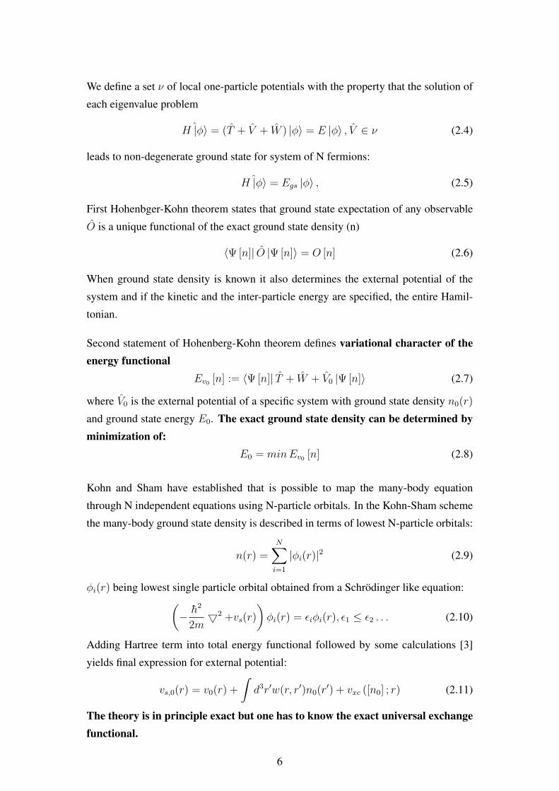
We define a set ν of local one-particle potentials with the property that the solution of

each eigenvalue problem

ˆH |φ〉 = (T + V + W ) |φ〉 = E |φ〉 , V ∈ ν (2.4)

leads to non-degenerate ground state for system of N fermions:

ˆH |φ〉 = Egs |φ〉 , (2.5)

First Hohenbger-Kohn theorem states that ground state expectation of any observable

O is a unique functional of the exact ground state density (n)

〈Ψ [n]| O |Ψ [n]〉 = O [n] (2.6)

When ground state density is known it also determines the external potential of the

system and if the kinetic and the inter-particle energy are specified, the entire Hamil-

tonian.

Second statement of Hohenberg-Kohn theorem defines variational character of theenergy functional

Ev0 [n] := 〈Ψ [n]| T + W + V0 |Ψ [n]〉 (2.7)

where V0 is the external potential of a specific system with ground state density n0(r)

and ground state energy E0. The exact ground state density can be determined byminimization of:

E0 = minEv0 [n] (2.8)

Kohn and Sham have established that is possible to map the many-body equation

through N independent equations using N-particle orbitals. In the Kohn-Sham scheme

the many-body ground state density is described in terms of lowest N-particle orbitals:

n(r) =N∑i=1

|φi(r)|2 (2.9)

φi(r) being lowest single particle orbital obtained from a Schrodinger like equation:(− h2

2m52 +vs(r)

)φi(r) = εiφi(r), ε1 ≤ ε2 . . . (2.10)

Adding Hartree term into total energy functional followed by some calculations [3]

yields final expression for external potential:

vs,0(r) = v0(r) +

∫d3r′w(r, r′)n0(r

′) + vxc ([n0] ; r) (2.11)

The theory is in principle exact but one has to know the exact universal exchangefunctional.

6

2.3 Basics of GW

Most of quantum chemistry approaches use a diagrammatic expansion of the elec-

tronic interactions through the bare Coulomb potential, which makes the inclusion of

electronic correlations extremely computationally demanding. The method described

in this section was first presented by Lars Hedin in 1965 [7] and is often referred as

the GW approximation. Conversely to quantum chemistry approaches [20] GW uses

an expansion on the screened Coulomb potential where the screening is calculated

through linear response.

To form a complete set for N-body system one would have to acquire all Slater deter-

minant from single particle functions. Notation that specifies states by listing quantum

labels k1, k2, . . . , kN is introduced:

(N)−1/2det uk(xl) ≡ |k, k1, k2, . . . , kN〉 (2.12)

”Creation/annihilation” operators a+k /ak are defined as:

a+k |k1, k2, . . . , kN〉 = |k, k1, k2, . . . , kN〉

ak |k1, k2, . . . , kN〉 = |k, k1, k2, . . . , kN〉(2.13)

It is also important to mention that

ak |k1, k2, . . . , kN〉 = 0 (2.14)

For k 6= ki for all i. From these definitions rest of commutation relations can be

deduced:[ak, a

+k′

]+

= aka+k′ + a+k′ak = δkk′ , [ak, ak′ ]+ =

[a+k , a

+k′

]+

= 0 (2.15)

In purpose of shortening notation and not applying a+k /ak to individual one-electron

states wave field operators ψ(x) and ψ+(x) are defined by:

ψ(x) =∑k

akuk(x) (2.16)

Where x stands for space and spin degrees of freedom. For the interpretation of

the many-body problem describing electrons interacting with each others we define

a Hamiltonian H that contains two terms: The ground state H0 and a perturbing term

H1. φ(x, t) represents small external perturbing potential.

H = H0 +H1

H0 =

∫Ψ+(x)h(x)Ψ(x)dx +

1

2

∫Ψ+(x)Ψ+(x′)v(r, r′)Ψ(x′)Ψ(x)dxdx′

H1 =

∫Ψ+(x)Ψ(x)φ(x, t)dx

(2.17)

7

The annihilation operator Ψ(x, t) satisfies the equation of motion:

i∂Ψ(x, t)∂t

= [h(x) + φ(x, t)] Ψ(x, t) +

∫v(r, r′)Ψ+(x′, t)Ψ(x′, t)Ψ(x, t)dx′ (2.18)

Using the relation dΘ(t)/dt = δ(t) and the commutation rules at equal times for

Ψ(x, t) and Ψ+(x, t) we obtain for the one electron Green function

[i(∂/∂t)− h(x)− φ(x, t)]G(xt, x′t′)

+i

∫v(r,r′′)dx′′ 〈N |T

Ψ+(x′′, t)Ψ(x′′, t),Ψ(x, t),Ψ+(x′, t)

|N〉

= δ(x, x′)δ(t, t′)

(2.19)

This terms with four field operators contains two particle Green function and describes

two-body correlations in the system. This equation can be used as basis for forming

infinite chains for more complicated correlations.

To describe interaction of a particle with the rest of the system we generalize the nota-

tion with the introduction of a nonlocal time (or energy) dependent quantity called the

self-energy operator Σ which is defined from equation 2.19 as:

[i(∂/∂t)− h(x)− V (x, t)]G(xt, x′t′)

−∫

Σ(xt, x′′t′′)G(x′′t′′, x′t′)dx′′dt′′ = δ(x, x′)δ(t, t′)(2.20)

The quantity V (x, t) is the total average potential in the system:

V (x, t) = φ(x, t) +

∫v(r, r′) 〈N |Ψ+(x′t)Ψ(x′, t) |N〉 dx′ (2.21)

It is more convenient to use frequency domain when dealing with energies hence the

Fourier transform:

G(x, x′;ω) =

∫G(xt, x′t′)exp [iω(t− t′)] d(t− t′) (2.22)

This expression is not valid unless G depends only on time arguments, implying time

independence (or zero value) of external potential φ(x, t). Fourier transform of self

energy operator 2.20 becomes

[ω − h(x)− V (x)]G(x, x′;ω)−∫

Σ(x, x′′;ω)G(x′′, x′;ω) = δ(x, x′) (2.23)

which represents many-body character of G origins in energy dependence of the self-

energy Σ. If it did not depend on energy the set of equations could be solved for a set of

eigenfunctions uk. Since this in not the case one has to look for physically meaningful

approximations. One of the most commonly used relatively simple estimations that

8

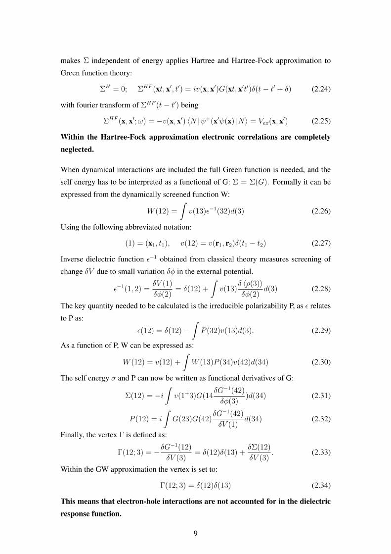
makes Σ independent of energy applies Hartree and Hartree-Fock approximation to

Green function theory:

ΣH = 0; ΣHF (xt, x′, t′) = iv(x, x′)G(xt, x′t′)δ(t− t′ + δ) (2.24)

with fourier transform of ΣHF (t− t′) being

ΣHF (x, x′;ω) = −v(x, x′) 〈N |ψ+(x′ψ(x) |N〉 = Vex(x, x′) (2.25)

Within the Hartree-Fock approximation electronic correlations are completelyneglected.

When dynamical interactions are included the full Green function is needed, and the

self energy has to be interpreted as a functional of G: Σ = Σ(G). Formally it can be

expressed from the dynamically screened function W:

W (12) =

∫v(13)ε−1(32)d(3) (2.26)

Using the following abbreviated notation:

(1) = (x1, t1), v(12) = v(r1, r2)δ(t1 − t2) (2.27)

Inverse dielectric function ε−1 obtained from classical theory measures screening of

change δV due to small variation δφ in the external potential.

ε−1(1, 2) =δV (1)

δφ(2)= δ(12) +

∫v(13)

δ 〈ρ(3)〉δφ(2)

d(3) (2.28)

The key quantity needed to be calculated is the irreducible polarizability P, as ε relates

to P as:

ε(12) = δ(12)−∫P (32)v(13)d(3). (2.29)

As a function of P, W can be expressed as:

W (12) = v(12) +

∫W (13)P (34)v(42)d(34) (2.30)

The self energy σ and P can now be written as functional derivatives of G:

Σ(12) = −i∫v(1+3)G(14

δG−1(42)

δφ(3))d(34) (2.31)

P (12) = i

∫G(23)G(42)

δG−1(42)

δV (1)d(34) (2.32)

Finally, the vertex Γ is defined as:

Γ(12; 3) = −δG−1(12)

δV (3)= δ(12)δ(13) +

δΣ(12)

δV (3). (2.33)

Within the GW approximation the vertex is set to:

Γ(12; 3) = δ(12)δ(13) (2.34)

This means that electron-hole interactions are not accounted for in the dielectricresponse function.

9

2.4 DFT in practice

The introduction of DFT has been briefly covered in section 2.2. The general idea of

the approach is provided by the set of Kohn-Sham equations in 2.9, 2.10 and in 2.11.

Looking at the equations it seems that the determination of the ground-state electronic

density is an easy task. However, their practical implementation requires the use of

some tricks and approximations [8].

2.4.1 Approximation to exchange functional

The Kohn-Sham equations represent a mapping of the interacting many-electron onto a

system of non-interacting electrons in the effective potential produced by all the other

particles. Complete knowledge of universal exchange correlation energy functional

would produce exact total density. However as the universal functional is unknown,

approximations have to be used. The most common drawback of these approximate

functionals is an over-counting of the electron-electron self-interaction in the Hartree

term.

One of the first used approximations is Local Density Approximation (LDA), which

states that exchange-correlation energy functional can be approximated by the one of

the homogeneous electron gas:

εXC(r) ≈ εhomXC [n(r)] . (2.35)

Various methods exist for exchange-correlation energy calculation from homogeneous

electron gas that give similar accuracy. They are all based on some parametrization

and are formulated to compute global minimum of the system. In all our calculationswe have used Perdew-Zunger LDA functional [25].

2.4.2 Plane wave expansion and Bloch theorem

Problem of dealing with multiple non-interacting electrons moving in static back-

ground potential is covered by Bloch theorem, which states that in a periodic lattice,

wave function can be written as a periodic part and a wavelike part [6]:

ψi(r) = expikrfi(r). (2.36)

10

The cell-periodic part becomes:

fi(r) =∑G

ci,GexpiGr, (2.37)

where G are reciprocal lattice vectors defined as G · l = 2πm. l are lattice vectors and

m integers. In full form electronic wave functions are expressed as:

ψi(r) =∑G

ci,k+G exp [i(k + G · r)] (2.38)

In principle an infinite set of plane vectors is needed. However coefficients ci,k+G for

plane waves with smaller kinetic energy (h2/2m)|k + G|2 are usually more important.

A cut off value can be used to truncate the basis set. This approximation allows a

description of wave functions with a discrete set of plane waves, i.e. with a finite basis

set. Convergence has to be checked with respect to this cut-off. A correction factor

can be calculated [11] for estimating the difference between theoretical infinite number

and practical finite basis sets.

Inserting plane wave function 2.38 into Kohn-Sham equation 2.10 followed by inte-

gration over r greatly simplifies expression:

∑G′

[h2

2m|k + G|2δGG’ + Vion(G−G′)

+VH(G−G′) + Vxc(G−G′)

]ci,k+G′ = εici,k+G

(2.39)

In this form kinetic energy term is diagonal and potential are described in terms of their

Fourier transforms. Size of the matrix depends on the cutoff energy (h2/2m)|k+Gc|2.

One of the Bloch theorem limitations is its description of defects or effects in direction

perpendicular to the lattice. In case of defects one must assume super-cell containing

defects and not every single defect in lattice. It is essential to include a bulk large

enough so the defects do not interact with each other.

2.4.3 The pseudo potential approximation

In practice plane-wave basis set provides very limiting platform for computation of

all-electron structure in real crystal as this would require extremely large cut-off for

describing the strongly oscillating electronic wave functions in the core region. The

pseudo potential approximation allows the electronic wave functions to be build from

11

much smaller basis set. The basis for this approximation comes from the fact that most

of the physical and chemical properties of materials depends on the valence electrons.

Thus effect of core levels are replaced by weaker pseudo potentials that act on set of

pseudo wave functions rather than the true valence wave functions. Pseudo potential is

build in such a way that scattering properties or phase shifts for pseudo functions are

identical to core level electrons and ion interaction, but with no remaining radial nodes

in the core region. The most general form of pseudo potential is:

VNL =∑lm

|lm〉Vl 〈lm| (2.40)

where |lm〉 are the spherical harmonics and Vl is the pseudo potential for angular mo-

mentum l. This operator decomposes the wave function into spherical harmonics, each

one is then multiplied with the relevant pseudo potential Vl. Local pseudo potential

means that same angular momentum components are used in a system. It is possi-

ble to produce predetermined phase shifts for each state but limitations arises with the

number of those shifts maintaining sufficient smoothness. Without a smooth and weak

pseudo potential, it becomes difficult to expand the wave functions using reasonable

number of plane-wave basis states. It is important that not only spatial dependences

of real and pseudo functions are the same but also absolute magnitudes in order to

produce same charge densities.

Total ionic potential of the solid is obtained by placing a pseudo potential at the position

of each ion. Information about positions can be expressed in the terms of the structure

factor for each wave vector G at atomic position RI :

Sα(G) =∑I

exp [iG · RI ] (2.41)

where the sum runs over all positions of defined specie α in single unit cell. Periodicity

of the system restricts nonzero components to reciprocal lattice vectors.

Total ionic potential Vion is formulated as a product of the structure factor and pseudo

potential over all the atomic species:

Vion(G) =∑α

Sα(Gvα(G)) (2.42)

At large distances pseudo potential is reduced to bare Coulomb potential (Z/r where

Z is the valence of the atom). More interesting is the behavior for small wave vectors

as it follows from Fourier transform that pseudo potential diverges as Z/G2. But since

it does not behave as pure Coulomb potential for small values it can be treated as

difference between the two. For a certain atomic specie ionic potential becomes:

vα,core =

∫ [Z/r − v0α(r)

]4πr2dr (2.43)

12

with v0α is pseudo potential for l = 0 angular momentum. This integral is nonzero only

within core region because the potentials are identical outside. There is no contribution

to total energy from Z/G2 component at G=0 due to cancellation of divergence but the

non-Coulomb part contributes with:

NelΩ−1∑α

Nαvα,core (2.44)

where Nel is the number of electrons in the system, Nα is total number of particular

specie’s atoms and Ω volume of the unit cell.

2.4.4 Ewald summation

The Coulomb energy is difficult to calculate using either real or reciprocal space as the

interaction is always long range. Ewald developed a rapidly convergent method for

Coulomb summation over a periodic lattice:∑l

1

|Rl + l − R2|=

2√π

∑l

∫ ∞η

exp[−|R1 + l − R2|2ρ2

]dρ+

2π

Ω

∑G

∫ η

0

exp

[−|G|

2

4ρ2

]exp [i(R1 − R2) ·G]

1

ρ3dρ

(2.45)

where l are the lattice vectors, G reciprocal-lattice vectors and Ω volume of the unit

cell. This identity rewrites the lattice summation for the Coulomb energy between

ion position on R2 and an array of atoms placed at the points R1 + l. It holds for all

the positive η. At first sight the infinite summation has been replaced by two sums,

one over real and other for reciprocal space. However it has property of much faster

convergence in personal space when applied with correct η. Yet there is a problem,

as the separation of sum into two spaces does not give the exact value of final total

energy. So additional terms need to be included into equation 2.45.

Eion =1

2

∑I,J

ZIZJe2

[∑l

erfc(η|R1 + l − R2|)|R1 + l − R2|

− 2η√ρδIJ+

4π

Ω

∑G 6==0

1

|G2|exp

−|G|

2

4η2

cos [(R1 − R2) ·G]− π

η2Ω

] (2.46)

where ZI and ZJ are the valences of the ions I and J. Erfc is complementary error

function. As ions do not interact with their own Coulomb charge, l = 0 term must be

omitted from the real space when I=J.

13

2.4.5 Born-Oppenheimer approximation

Since now, we have only presented the approximations that are used for the electronic

degree of freedom, assuming that the ions are frozen at a given position. When mod-

eling material properties, however, one needs to take into account also atomic relax-

ations. The knowledge of the ground-state of a system implies the finding of the global

minimum of the system, including both electrons and ions. In principle, this search

needs the solution of a quantum equation where the electronic and ionic degrees of

freedom are entangled. However, as the mass of electrons is insignificant compared

to ionic masses it can be assumed that electrons will instantly respond to any atomic

movement. This assumption is called the Born-Oppenheimer approximation and al-

lows for the separation of electronic and nuclear wave functions:

Ψtotal = ΨelectronicΨnuclear (2.47)

Moreover, as most of the atomic elements have a De Broglie wave-length very small,

the atomic degrees of freedom are always treated classically. The finding of the ground

state then is implemented with two loops: the internal one, search for the electronic

ground-state at fixed ionic positions, the external one, solve classical Newton equa-

tions for the ions. These were some of the fundamental approaches and approximation

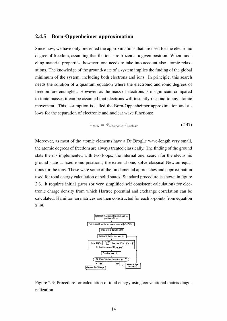
used for total energy calculation of solid states. Standard procedure is shown in figure

2.3. It requires initial guess (or very simplified self consistent calculation) for elec-

tronic charge density from which Hartree potential and exchange correlation can be

calculated. Hamiltonian matrices are then constructed for each k-points from equation

2.39.

Figure 2.3: Procedure for calculation of total energy using conventional matrix diago-

nalization

14

Kohn-Sham eigenvalues are calculated from diagonalization of this matrix. This pro-

cedure is used until convergence is achieved. Total energy usually depends more on the

ionic potential than configuration potential so calculations are performed using an en-

ergy cutoff and number of k points at which energy differences have converged rather

than absolute energy convergence.

2.5 GW in practice

Foundations of GW approximation [2] [7] have been described in the section 2.3. GW

approach can be seen as generalized Hartree-Fock where correlations are taken into

account through linear response. Basic equations are too difficult (or time consuming)

for practical use in their original form, so again some tricks and approximations are

used.

We begin with the assumption of a periodic system with unit cell of volume Ω, set up

by N number of cells, such as limit goes to N →∞. Every function is represented as

sum of normalized plane waves and depends on spatial coordinates.

Ψnk(x) =1√NΩ

∑G

ψnk(G)ei(k+G)x (2.48)

Where G runs over reciprocal lattice. Products of the two Kohn-Sham states in real

space is:

Mnk,n′,k′(x) =√NΩψ∗nk(x)ψn′,k′(x) (2.49)

Preferably functions are expressed in phase space and require Fourier transformation.

For example polarizabitliy becomes:

P (xx′;ω) =1

NΩ

∑kGG′

ei(k+G)xPk(G,G′;ω)e−i(k+G

′)x’ (2.50)

Sum over k vectors runs through a set of uniformly spaced points in first Brillouin

zone. Same convention is used for bare Coulomb potential vc resulting in reciprocal

spaced diagonal matrix:

vc(x, x′) =2

|x− x′|(2.51)

vck(G,G′) =

8π

(G+ q)2δGG′ (2.52)

The first step for GW calculation is evaluation of polarizability P0. Only the imaginary

value of frequency is included: ω = is. The expression in reciprocal space is:

Pq(GG′; is) = − 4

NΩ

∑cvqk

θ(εck − µ)θ(µ− εvk+q)M∗ck,vk+q(G

′)

2(εck − εvk+q)(εck − εvk+q)2 + s2

(2.53)

15

µ in the Fermi energy, so the θ function selects a band index v, which belongs to

occupied bands (valence) and bands c representing unoccupied states (conduction).

Ideally sums over k and q should be performed over infinitely dense mesh in first

Brillouin zone. In practice special points technique is used: Fourier quadrature of the

integrand. It is also useful to consider analytical behavior of P when q → 0 as:

Pq(G = 0, G′ = 0;ω)∑αα′

qαSαα′

(ω)qα′ (2.54)

Pq(G,G′ = 0;ω)

∑α

Lα(G;ω)qα (2.55)

Pq(G = 0, G′;ω)∑α

qα(Rα(G′;ω))∗ (2.56)

where α and α′ run over three spatial coordinates. For imaginary frequencies P is

Hermitian.

Second step is to compute screened Coulomb potential, obtained as:

W (is) = [1− νcP (is)]−1 νc (2.57)

For imaginary frequencies W is Hermitian as well. We split the screened Coulomb

potential into pure exchange and pure correlation by subtracting vc. This way the

exchange self-energy is given by:

〈nk|Σx |n′k〉 = − 1

NΩ

∑vq

∑G

θ(µ− εvk−q)M∗vk−q,nk(G)vcq(G)Mvk−q,n′k(G) (2.58)

and correlation by:

〈nk|Σc(ω) |n′k〉 = − 1

NΩ

∑n”q

∑GG′

M∗n”k−q,nk(G)Mn”k−q,n′k(G

′)

−1

2πi

∫dω′

W PGG′(q;ω′)e

−iδω′

ω + ω′ − εn”k−q − iηsign(µ− εn”k−q)

(2.59)

Setting σc to zero will give Hartree-Fock approximation. This integral is problematic

to solve and computationally demanding for systems with more than a few electrons.

Usually plasmon-pole models are used for the screening. In our calculations we have

used the Godby-Needs [24] plasmon-pole that allows for an analytical solution of the

energy integral.

2.5.1 The plasmon-pole model

The dynamical behavior of the dielectric matrix is given by a parametrized model of

the dielectric function in reciprocal space:

ε−1GG′(q;ω) = δGG′ +Ω2GG′(q)

ω2 − ωGG′(q)2(2.60)

16

where ΩGG′ (effective bare plasma frequency) and ωGG′ are the two parameters of the

model. These frequencies are chosen, when ε−1 is actually computed, as: ω = 0

and ω = iωp (ωp is an estimate for plasmon frequency). This should only work,

in principle, for systems where plasmons are well defined. However, it has been also

applied to molecules and has given very accurate results. Once the screening is known,

the correlation part of self energy from equation 2.59 can be evaluated analytically by

choosing an integration part with an arc in the lower half plane (e−iδω′). We obtain:

−1

2πi

∫dω′

W PGG′(q;ω′)e−iδω

′

ω + ω′ − εn”k−q − iηsign(µ− εn”k−q)=

−1

2πi

∫dω′

(ε−1GG′(q;ω′)− δGG′)vC(G′ + q)e−iδω′

ω + ω′ − εn”k−q − iηsign(µ− εn”k−q)=

−∆2GG′vC(G′ + q)

2δGG′(q)

[θ(µ− εnk)

ω + ωGG′(q)− εnk − iη+

θ(εnk − µ)

ω + ωGG′(q)− εnk + iη

] (2.61)

2.5.2 Perturbative GW, GW@DFT

The most important computational approximation is that, even if in principle GW equa-

tions form a set of complete equations that should be solved self-consistently, this is

almost never achieved. Indeed in the majority of the cases, it is sufficiently accurate

(and computationally affordable) to perform a one-shot GW on top of some reason-

able DFT initial guess. In other words, the DFT initial wave functions are assumed

to be very close to the ”real” quasi-particle wave functions and are not re-calculated,

while DFT Kohn-Sham energies are corrected with a diagonal GW self-energy. In the

literature this approximation is often referred as GW@DFT or G0W0. As the GW cor-

rection does not come from a diagonalization, and DFT exchange-correlation poten-

tials fail in describing energy differences between electronic states of different nature

(delocalized-localized, occupied un-occupied) some times a change in the energy or-

dering of the states may appear between DFT and GW@DFT. In all our calculationswe have performed G0W0 on top of DFT-LDA.

2.6 Bethe-Salpeter equation

Eigenstate |E〉 and energy Ω of ”unknown” excitonic state can be calculated from [12]:

H |E〉 = Ω |E〉 (2.62)

|E〉 can be written in the basis of single-particle orbitals as:

Ψ(xx′) =∑nn′k

ψqpnk(x)ψqp∗n′k(x′) (2.63)

17

Excitation energies are solution of an eigenvalue problem and it is necessary to find a

form of effective two-particle Hamiltonian of eq. 2.62. In the context of neutral exci-

tations, this effective two-particle Hamiltonian is called the Bethe-Salpeter equation,

describing electron-hole pairs.

The information about this excitation is given as two-particle Green-Function:

G2(x1t1, x2t2, x3t3, x4t4) = (−i)2 〈N |TΨ(x1t1)Ψ(x2t2)Ψ†(x3t3)ψ † (x4t4) |N〉

(2.64)

G2 describes the propagation of created electron-hole pair and |N〉 is the ground state

of N particle system.

Four point independent particle polarizability from equation 2.32 is:

P 0(1, 1′; 2, 2′) = −iG(1′, 2′)G(2, 1) (2.65)

Generalized form for response function is then:

χ(1, 1′, 2, 2′) = P0(1, 1′, 2, 2′) +

∫P0(1, 1

′, 3, 3′)[v(3, 3′, 4, 4′)

−W (3, 3′, 4, 4′)]P (4, 4′, 2, 2′)d3d3′d4d4′(2.66)

Expression for polarizability differs only in term of long range Coulomb potential

(v → v).

In practice all of the quantities are calculated in frequency domain thus requiring

Fourier transform:

χ(1, 1′, 2, 2′) = χ(x1t1, x′1t†1, x2t2, x

′2t†2)→ χ(x1, x

′1, x2, x

′2, ω)δ(x1 − x′1)δ(x2 − x′2)

(2.67)

Another important assumption implemented is energy dependence of the screen poten-

tial which is neglected assuming W (ω) = W (ω = 0). In theory this could be solved

with inverting the matrix for each possible frequency ω. However there exists more

practical way, reformulating the problem into effective eigenvalue problem. First step

consists of changing the basis set, consisting of single particle eigenfunctions ψn(x)

(the subindex n has to be read as n = (n, k), it now contains the information of the

band and k point). In this basis four point quantities become:

S(x1, x1′ , x2, x2′) =∑

(n1,n1′ )(n”,n2′ )

ψ∗n1(x1)ψn′

1(x′1)ψn2(x2)φ

∗n2

(x2′)S(n1,n1′ )(n2,n2′ )

(2.68)

Active eigenvalue problem now becomes:∑(n1,n1′ )(n2,n2′ )

H(n1,n1′ )(n2,n2′ )2pAµ(n2,n2′ )

= EµAµ(n2,n2′ )(2.69)

18

where two-particle Hamiltonian is:

H(n1,n1′ )(n2,n2′ )2p = (εn1′

− εn1)δ(n1,n2)(n1′ ,n2′ )+ (fn1 − fn1′

)Ξ(n1,n1′ )(n2,n2′ )(2.70)

with εn1′and εn1 being quasi particle energy eigenvalues and Ξ(n1,n1′ )(n2,n2′ )

presenting

the interaction kernel, defined as:

Ξ(n1,n2′ )(n2,n2′ )= −

∫dx1dx1′ψn1ψ

∗n1′

(x1′)W (x1, x1′)ψ∗n2

(x1)ψn2′(x1)

+

∫dx1dx1′ψn1(x1)ψ

∗n1′

(x1)v(x1, x1′)ψ∗n2

(x1′)ψn2′(x1′)

(2.71)

In general Aµ are not orthogonal. In the case of semiconductors this expression can be

simplified: (fn1 − fn1′) is different from zero only for transitions for which (n1, n1′)=

(occupied, unoccupied) or vice versa.

The matrix representation of the two body Hamiltonian for a semiconductor-insulator

is:

vc, c2 c2, v2 v2, v2′ c2, c2′

v1, c1 H2p(v1c1)(v2c2)

Ξ(v1c1)(c2v2′ )Ξ(v1c1)(v2v2′ )

Ξ(v1,c1)(c2c2′ )

c1, v1 −Ξ(c1,v1)(v2c2) −H2p(c1v1)(c2v2)

−Ξ(c1v1)(v2v2′ )−Ξ(c1v1)(c2c2′ )

v1, v1′ 0 0 evδ(v1,v2)(v1′ ,v2′ ) 0

c1, c1′ 0 0 0 ecδ(c1,c2)(c1′ ,c2′ )

(2.72)

where ev = (Ev1′ − Ev1) and ec = (Ec1′ − Ec1). vi and ci stand for valence and

conduction states, respectively.

In ”block” representation matrix for H2p is: H2p−resonant(v1c1)(v2c2)

Ξcoupling(v1c1)(c2v2)

−[Ξcoupling(v1c1)(c2v2)

]∗−[H2p−resonant

(v1c1)(v2c2)

]∗ (2.73)

H2p−resonant is Hermitian and corresponds to positive absorption energy while− [H2p−resonant]

gives de-excitation energies. Ignoring the coupling part of the matrix eigenvalue prob-

lem is reduced to: ∑(v2,c2)

Hexc,2p resonant(v1,c1)(v2,c2)

Aµ(v2,c2) = Eexcµ Aµ(v1,c1) (2.74)

This resonant part is the one that is diagonalized in all our calculations.

19

3. Peroxy linkage defect in silica

It has been briefly commented in the introduction that previous works on the optical

properties of POL are scarce and the results quite controversial [13].

Experimentally only very few results report peroxy bridge measurements. In one case

it has been assigned to a very broad peak in the 6.5-7.8 eV region [17], while ref.

[26] reports a band at 3.8 eV with a very low intensity. Ref. [26] and [17] justify

the presence of POL with absence of any EPR signals because POL defect is indeed

a paramagnetic defect. Their second argument is the decrease of the observed optical

absorption peak after hydrogen treatment, possibly due to following reaction:

≡ Si - O - O - Si ≡ +H2 →≡ Si - O - H + H - O -Si ≡ (3.1)

First theoretical estimation was proposed by O’Reilly and Robertson [15]. They used

a tight-binding Hamiltonian model on a 243 atoms α-quartz cell. Peroxy bridge con-

figuration was considered to be the same as in the H2O2 molecule: 1.49 A distance

between O atoms and dihedral angle between O-O-H of approximately 100. This first

attempt is, of course, very rough as it is well known that tight-binding like methods

completely miss the description of solid-state effects, which are crucial in bulk mate-

rials. The simple use of the crystalline polymorph quartz may not be too bad, as the

local structure of quartz and a-SiO2 is very similar. Indeed, quartz and silica are based

on a network of SiO4 tetrahedral. In ref. [15], it is shown that POL induces two states:

a pσ resonance at -4.4 eV and an empty pσ∗ state at 4.2 eV, which produce optically

active transition at 8.6 eV. From the numbers, it is clear that electron-hole interaction

has completely been neglected. We expect that this electron-hole interaction would be

very important in silica, leading to strongly bounded excitons, as silica has a very low

dielectric constant.

G. Pacchioni and G. Ierano studied peroxy bridge defect in silica using the Hartree-

Fock (HF) approximation followed by various configuration interaction (CI) correc-

tions [13]. Calculations were performed on small cluster models passivated with H (the

20

biggest cluster was Si2O8H6). The use of cluster models precludes a correct treatment

of the long-range dielectric behavior of the system under study. Another limitation lies

in the use of localized basis sets for which the completeness of the basis can not be

stated a-priori, and consequently the results may strongly depend on the basis choice.

The relaxed distance between O-O atoms is 1.43 A. The results show that the lowest

transition occur at 6.5 ± 0.3 eV with a very low intensity approximately 10−4. It is

supposed to occur from doubly occupied π∗ orbital from just above oxygen 2p band

localized on O-O to the conduction band. This study does not show presence of an

empty σ∗ defect state, contrary to the model proposed by Robertson [15].

In ref. [13] there are also presented some calculations on the hydrogen peroxide

molecule that is used as a very simplify model for POL. Various configuration in-

teraction treatments show that the lowest transition occurs at (6.2±0.2) eV. As there

are no experimentally detected absorption bands below 6.7 eV, the only option is to

compare this result with other theoretical reports. In ref. [16] a similar transition en-

ergy (6.24 eV) has been calculated. In the case of molecules, we expect that the use of

localized basis may not give an accurate description of the optical transitions in H2O2,

as such basis completely fails in modeling scattering states. Scattering states may be

crucial when dealing with H2O2, as its electron affinity (EA) is negative. A negative

EA always induces the presence of scattering states between the vacuum level and the

lowest unoccupied molecular orbit (LUMO) .

In the last referred study [18], Time Dependent Density Functional Theory was used

with standard exchange-correlation functionals and with 20% fraction of Fock poten-

tial. It is well known that the accuracy of TDDFT can not be assessed a-priori, indeed

citing the authors of [18]: ”the absolute value are likely to be underestimated ... we

focus only on comparing the transition energies for the various sites ...”.

21

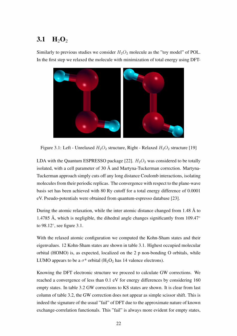
3.1 H2O2

Similarly to previous studies we consider H2O2 molecule as the ”toy model” of POL.

In the first step we relaxed the molecule with minimization of total energy using DFT-

Figure 3.1: Left - Unrelaxed H2O2 structure, Right - Relaxed H2O2 structure [19]

LDA with the Quantum ESPRESSO package [22]. H2O2 was considered to be totally

isolated, with a cell parameter of 30 A and Martyna-Tuckerman correction. Martyna-

Tuckerman approach simply cuts off any long distance Coulomb interactions, isolating

molecules from their periodic replicas. The convergence with respect to the plane-wave

basis set has been achieved with 80 Ry cutoff for a total energy difference of 0.0001

eV. Pseudo-potentials were obtained from quantum-espresso database [23].

During the atomic relaxation, while the inter atomic distance changed from 1.48 A to

1.4785 A, which is negligible, the dihedral angle changes significantly from 109.47

to 98.12, see figure 3.1.

With the relaxed atomic configuration we computed the Kohn-Sham states and their

eigenvalues. 12 Kohn-Sham states are shown in table 3.1. Highest occupied molecular

orbital (HOMO) is, as expected, localized on the 2 p non-bonding O orbitals, while

LUMO appears to be a σ* orbital (H2O2 has 14 valence electrons).

Knowing the DFT electronic structure we proceed to calculate GW corrections. We

reached a convergence of less than 0.1 eV for energy differences by considering 160

empty states. In table 3.2 GW corrections to KS states are shown. It is clear from last

column of table 3.2, the GW correction does not appear as simple scissor shift. This is

indeed the signature of the usual ”fail” of DFT due to the approximate nature of known

exchange-correlation functionals. This ”fail” is always more evident for empty states,

22

Table 3.1: Kohn-Sham eigenvalues and square modulus of the corresponding wave-

function. O atoms are in red and H atoms in blue

Band EigenValue Plot Band Eigen Value Plot

1 -27.79 eV 2 -22.34 eV

3 -13.01 eV 4 -12.57 eV

5 -9.60 eV 6 -9.034 eV

7-HOMO -5.90 eV 8-LUMO -1.87 eV

9 -0.80 eV 10 0.110 eV

11 0.111 eV 12 0.47 eV

of course, as DFT deals with electronic density and hence with ”occupied states”.

Experimentally no data exists for the Electron Affinity (EA) of hydrogen peroxide, as it

has a negative electron-affinity. Quantum Chemistry theoretical calculations place the

EA at -2.5 eV [28]. Many scattering states will be present between LUMO and vacuum

level such enabling more complex electronic transitions. Experimental measurements

of vertical ionization potential (VIP) placed it around 11.6 eV [30] [31]. Theoretical

calculations have shown that the VIP value strongly depends on the dihedral angle

[27]. With these two values for IP and EA we can estimate the HOMO-LUMO gap for

H2O2 to be around 14 eV. Within GW we obtained a HOMO-LUMO gap of 13.3 eV,

which is in very good agreement with the few results available in the literature.

GW has provided with the N-1 and N+1 electronic excitations. We proceeded with the

solution of Bethe-Salpeter equation. The imaginary part of the macroscopic dielectric

tensor, molar absorptivity (related to the absorption spectra), is calculated from exci-

tonic oscillator strength (probability of coupling with light), see figure 3.2. Results

containing first four transitions are shown in Table 3.3. The lowest excitonic transition

23

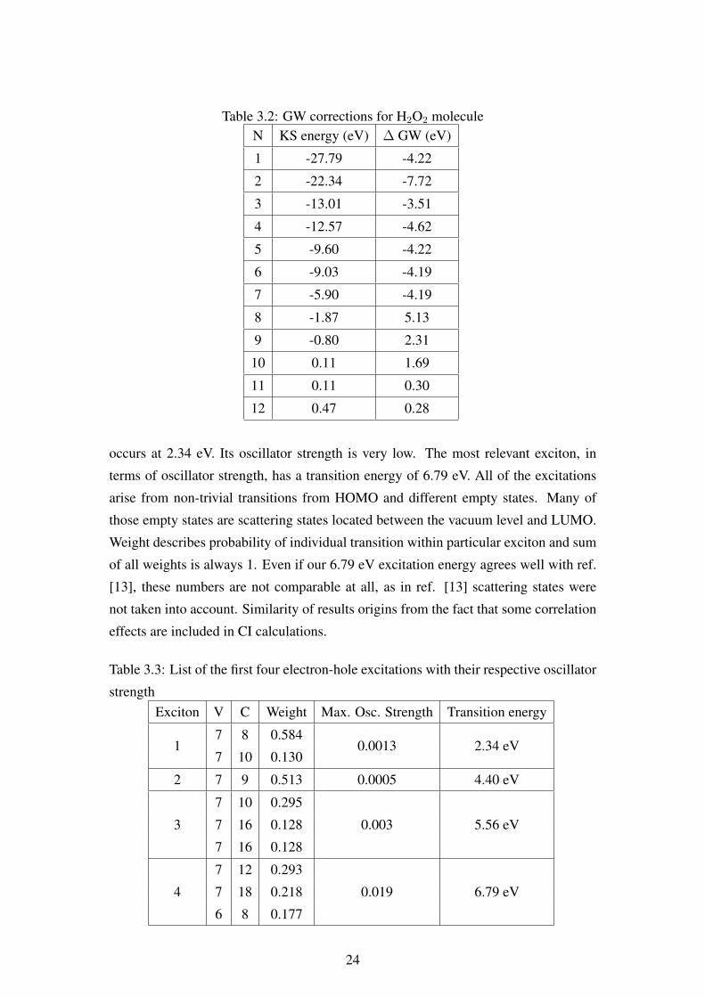
Table 3.2: GW corrections for H2O2 moleculeN KS energy (eV) ∆ GW (eV)

1 -27.79 -4.22

2 -22.34 -7.72

3 -13.01 -3.51

4 -12.57 -4.62

5 -9.60 -4.22

6 -9.03 -4.19

7 -5.90 -4.19

8 -1.87 5.13

9 -0.80 2.31

10 0.11 1.69

11 0.11 0.30

12 0.47 0.28

occurs at 2.34 eV. Its oscillator strength is very low. The most relevant exciton, in

terms of oscillator strength, has a transition energy of 6.79 eV. All of the excitations

arise from non-trivial transitions from HOMO and different empty states. Many of

those empty states are scattering states located between the vacuum level and LUMO.

Weight describes probability of individual transition within particular exciton and sum

of all weights is always 1. Even if our 6.79 eV excitation energy agrees well with ref.

[13], these numbers are not comparable at all, as in ref. [13] scattering states were

not taken into account. Similarity of results origins from the fact that some correlation

effects are included in CI calculations.

Table 3.3: List of the first four electron-hole excitations with their respective oscillator

strengthExciton V C Weight Max. Osc. Strength Transition energy

17 8 0.584

0.0013 2.34 eV7 10 0.130

2 7 9 0.513 0.0005 4.40 eV

3

7 10 0.295

0.003 5.56 eV7 16 0.128

7 16 0.128

4

7 12 0.293

0.019 6.79 eV7 18 0.218

6 8 0.177

24

Figure 3.2: Plot of the absorption spectrum with respect to the photon energy. An

artificial broadening of 0.001 eV has been used.

3.2 Silica

To model the POL defect in silica, we have used a 108-atoms non-defective model

in which we have added an O atom. The silica model has been obtained through

quenching from a melt, see [29]. As the system is disordered with 72 oxygen sites,

there are 72 possible different configurations for inserting the additional O atom, see

figure 3.3.

Figure 3.3: Silica model with lowest formation energy. Silicon atoms are represented

in blue and oxygen atoms in red. Peroxy bridge defect is highlighted

25

The GW-BSE calculations are ”very expensive”: In order to have some statistic, but

saving computer time, we have only considered five different configurations containing

≡ Si - O - O - Si ≡ bridge defect. The total number of valence electrons is 582 (291

occupied states). The non-defective 108 atoms silica model is used as reference. All

the structures were fully relaxed with DFT-LDA [22]. After the atomic relaxation, the

average distance for -O-O- bond is 1.4994 A and for ≡ Si-O- bond 1.6707 A.

The POL DFT electronic structure is schematically represented in figure 3.4. POL

induces the creation of two strongly localized defect states in band gap. State 291 is

similar to the H2O2 HOMO, while 292 is similar to the LUMO (see table 3.1). The two

states are the defect -O-O- 2p and =O-O- σ* states, respectively. The energy difference

between this two states is 4.3 eV, very close to the DFT HOMO-LUMO gap of 4 eV for

H2O2. The 291 state is at 0.47 eV from the top of valence band (TVB), while 292 is at

4.77 eV. The DFT band gap is 5.49 eV (DFT always underestimates energy differences

between occupied and unoccupied states).

Figure 3.4: Schematic presentation of electronic structure in POL defect induced silica

One-shot GW calculation has been done on top of the previous DFT-LDA results.

Table 3.4 displays the difference of the two methods and results are schematically

shown in figure 3.5. We can quickly observe that the energies of states 292 and 293

have shifted and LUMO now appears in the conduction band. First defect state (291)

in positioned at 0.44 eV from the TVB. This value is very close to the 0.47 eV given

26

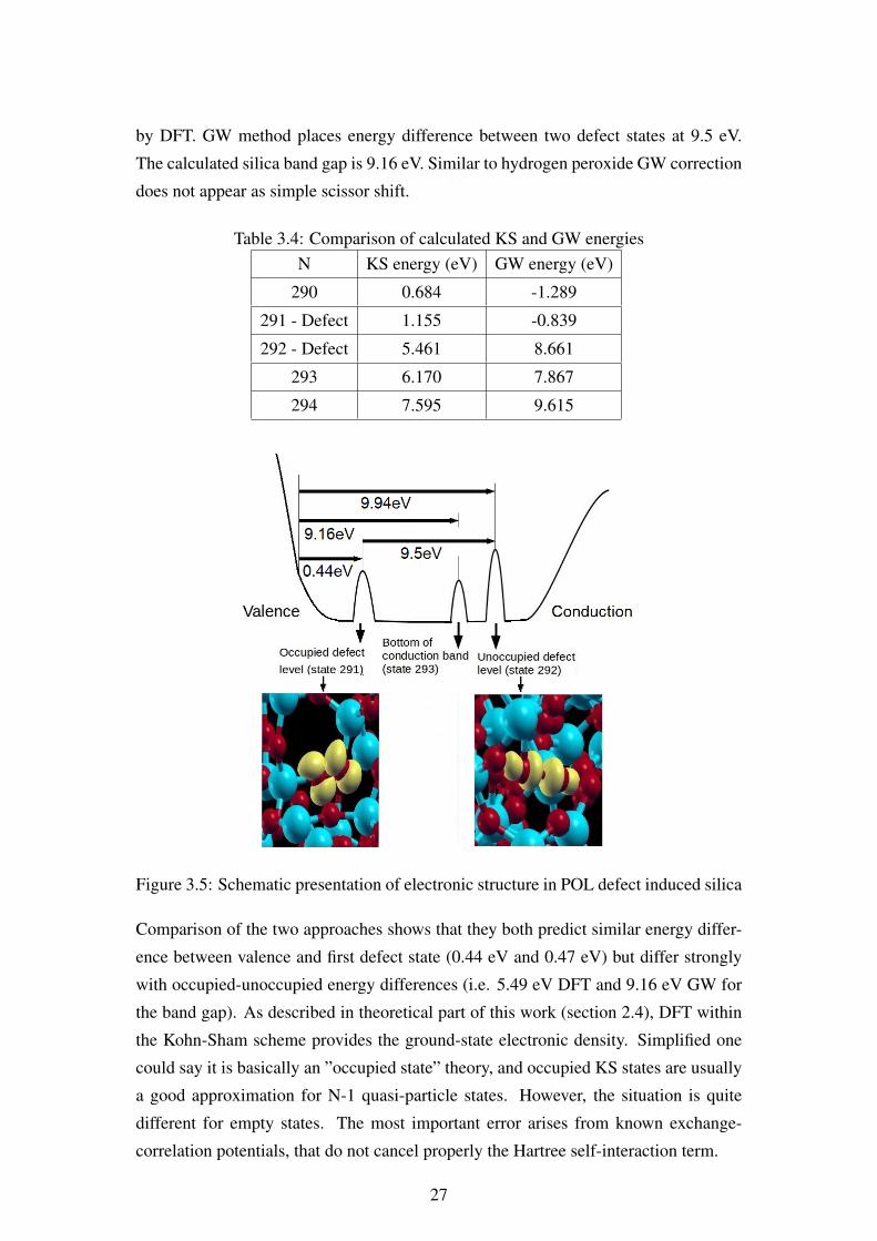
by DFT. GW method places energy difference between two defect states at 9.5 eV.

The calculated silica band gap is 9.16 eV. Similar to hydrogen peroxide GW correction

does not appear as simple scissor shift.

Table 3.4: Comparison of calculated KS and GW energiesN KS energy (eV) GW energy (eV)

290 0.684 -1.289

291 - Defect 1.155 -0.839

292 - Defect 5.461 8.661

293 6.170 7.867

294 7.595 9.615

Figure 3.5: Schematic presentation of electronic structure in POL defect induced silica

Comparison of the two approaches shows that they both predict similar energy differ-

ence between valence and first defect state (0.44 eV and 0.47 eV) but differ strongly

with occupied-unoccupied energy differences (i.e. 5.49 eV DFT and 9.16 eV GW for

the band gap). As described in theoretical part of this work (section 2.4), DFT within

the Kohn-Sham scheme provides the ground-state electronic density. Simplified one

could say it is basically an ”occupied state” theory, and occupied KS states are usually

a good approximation for N-1 quasi-particle states. However, the situation is quite

different for empty states. The most important error arises from known exchange-

correlation potentials, that do not cancel properly the Hartree self-interaction term.

27

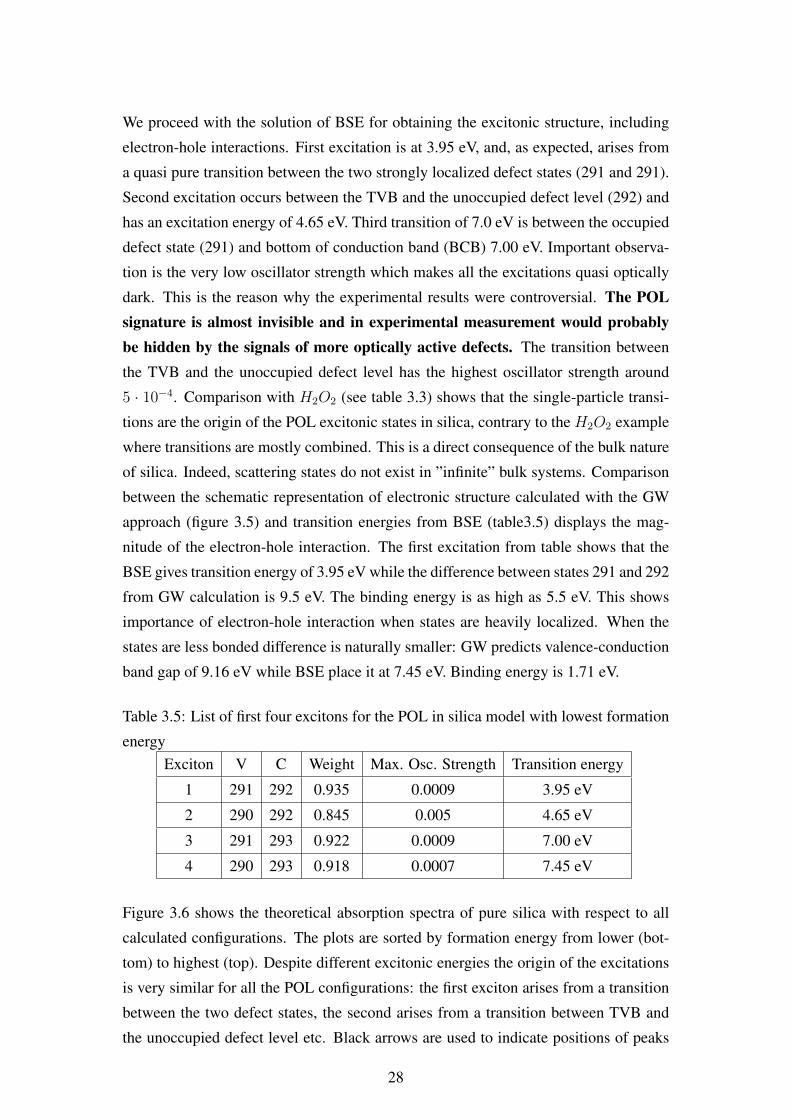
We proceed with the solution of BSE for obtaining the excitonic structure, including

electron-hole interactions. First excitation is at 3.95 eV, and, as expected, arises from

a quasi pure transition between the two strongly localized defect states (291 and 291).

Second excitation occurs between the TVB and the unoccupied defect level (292) and

has an excitation energy of 4.65 eV. Third transition of 7.0 eV is between the occupied

defect state (291) and bottom of conduction band (BCB) 7.00 eV. Important observa-

tion is the very low oscillator strength which makes all the excitations quasi optically

dark. This is the reason why the experimental results were controversial. The POLsignature is almost invisible and in experimental measurement would probablybe hidden by the signals of more optically active defects. The transition between

the TVB and the unoccupied defect level has the highest oscillator strength around

5 · 10−4. Comparison with H2O2 (see table 3.3) shows that the single-particle transi-

tions are the origin of the POL excitonic states in silica, contrary to the H2O2 example

where transitions are mostly combined. This is a direct consequence of the bulk nature

of silica. Indeed, scattering states do not exist in ”infinite” bulk systems. Comparison

between the schematic representation of electronic structure calculated with the GW

approach (figure 3.5) and transition energies from BSE (table3.5) displays the mag-

nitude of the electron-hole interaction. The first excitation from table shows that the

BSE gives transition energy of 3.95 eV while the difference between states 291 and 292

from GW calculation is 9.5 eV. The binding energy is as high as 5.5 eV. This shows

importance of electron-hole interaction when states are heavily localized. When the

states are less bonded difference is naturally smaller: GW predicts valence-conduction

band gap of 9.16 eV while BSE place it at 7.45 eV. Binding energy is 1.71 eV.

Table 3.5: List of first four excitons for the POL in silica model with lowest formation

energyExciton V C Weight Max. Osc. Strength Transition energy

1 291 292 0.935 0.0009 3.95 eV

2 290 292 0.845 0.005 4.65 eV

3 291 293 0.922 0.0009 7.00 eV

4 290 293 0.918 0.0007 7.45 eV

Figure 3.6 shows the theoretical absorption spectra of pure silica with respect to all

calculated configurations. The plots are sorted by formation energy from lower (bot-

tom) to highest (top). Despite different excitonic energies the origin of the excitations

is very similar for all the POL configurations: the first exciton arises from a transition

between the two defect states, the second arises from a transition between TVB and

the unoccupied defect level etc. Black arrows are used to indicate positions of peaks

28

as some are indeed so small that sometimes they cannot be even seen. Qualitatively

excitation 2 from table 3.5 appears to be the most probable POL induced transition

from all configurations. Some differences in transition energies are visible among dif-

ferent graphs. Qualitatively they can be estimated to shift transitions up to 1 eV. Their

origin is probably slight difference in POL defect geometry between different configu-

rations. Further research is needed to fully understand significance of defect geometry

to optical properties.

Figure 3.6: Absorption spectra of ”pure” silica and defect induced models. Black

arrows are used to indicate POL induced excitons that have very small oscillator

strengths.

29

4. Conclusion

In this work, we have studied from first-principles the opto-electronic properties of the

peroxy bridge defect in pure silica. We have used state-of-the art Density Functional

Theory with local density approximation, followed by GW@DFT and the solution of

the BSE. Through this combination of approaches we can model parameter-free N-1

and N+1 electronic and neutral excitations including polarization, solid state effects

and electron-hole interactions.

We have found that, there are three quasi-dark excitations at 3.95 eV, 4.65 eVand 7.00 eV and that can be bi-unequivocally associated to the POL. Howeveras they are quasi-dark, it is very difficult (almost impossible) to experimentallydistinguish the POL excitations from the background generated by other opti-cally active defects. This is the reason why previous experimental results werecontroversial. Previous theoretical works on the topic were giving misleading results

due to the intrinsic limitations of the methods that were used. Of course, at that time,

those approaches were the only possibility, as the needed computational resources for

addressing the issue of optical excitations in silica through GW and BSE are enor-

mous. Only recently such kind of calculations became possible on High Performance

Computing Facilities.

30

Bibliography

[1] A. Kordon, Aplying computational intelligence: How to create value, Springer

Science & Business Media, New York (2009)

[2] L. Hedin and S. Lundqvist, Solid state physics, Volume 23, Academic Press, New

York, London (1969)

[3] R. M. Dreizler, E. K. U. Gross, Density functional theory: An approach to the

quantum many-body problem, Springer-Verlag, Berlin (1990)

[4] D. Griffiths, Introduction to Quantum mechanics, Prentice Hall Inc., New Jersey

(1995)

[5] G. Baiagaluppi, A. Valentini, Quantum theory at the crossroads, Cambridge uni-

versity press (2009)

[6] N. W Ashcroft, N. D. Merminn, Solid state physics, Harcourt Inc. (1976)

[7] L. Hedin, Phys. Rev. 139 a796 (1965)

[8] M. C. Payne, M. P. Teter, D. C. Allan, T. A. Arias, J. D. Joannopoulos, Reviews of

modern physics 64, 1045 (1992)

[9] A. Pasquarello and Roberto Car, Phys. Rev. Lett. 80, 5145 (1998)

[10] J. F. Janak, Phys. Rev. B. 18, 7165 (1978)

[11] G. P. Francis, M. C. Payne, J. Phys: Condens. matter 17, 1643 (1990)

[12] L. M. Samos, G. Bussi, SaX: An open source package for electronic-structure

and optical properties calculations in the GW approximation, Computer physics

communications 180, 1416 (2009)

[13] G. Pacchioni, G Ieranom Phys. Rev. B 57, 818 (1998)

31

[14] C. Kittel, Introduction to Solid State Physics - 8th ed. Wiley, 2005

[15] E. O’Reilly and J. Robertson, Phys. Rev. B 27, 3780 (1983)

[16] A. Rauk, M. Barrel, Chem Phys. 25, 409 (1977)

[17] H. Imai, K. Arai, H. Hosono, Y. Abe, T. Arai and H. Imagawa, Phys. Rev. B 44,

1812 (1991)

[18] D. Ricci, G. Pacchioni, M. A. Szymanski, A. L. Shluger, A Marshall

Stoneham. Phy. Rev. B 65, 224104 (2001)

[19] A. Kokalj, Comp. Mater. Sci., 2003, Vol. 28, p. 155

[20] T. Helgaker, P. Jorgensen, J. Olsen, Molecular electronic structure, Wiley, 2000

[21] L. M. Samos, G. Bussi, et al, http://www.sax-project.com

[22] P. Giannozzi, S. Baroni, N. Bonini, M. Calandra, R. Car, C. Cavazzoni, D.

Ceresoli, G. L. Chiarotti, M. Cococcioni, I. Dabo, A. Dal Corso, S. Fabris, G.

Fratesi, S. de Gironcoli, R. Gebauer, U. Gerstmann, C. Gougoussis, A. Kokalj,

M. Lazzeri, L. Martin-Samos, N. Marzari, F. Mauri, R. Mazzarello, S. Paolini, A.

Pasquarello, L. Paulatto, C. Sbraccia, S. Scandolo, G. Sclauzero, A. P. Seitsonen,

A. Smogunov, P. Umari, R. M. Wentzcovitch, J. Phys. Condens. Matter 21, 395502

(2009).

[23] Quantum ESPRESSO pseudopotential data base: http://www.quantum-

espresso.org/pseudopotentials

[24] R. W. Godby, R. J. Needs, Phys. Rev. Lett. 62 (1989) 1169

[25] J. P. Perdew, A. Zunger, Phys. Rev. B 23, 5048 (1981)

[26] H. Nishikawa, R. Tahmon, Y. Ohki, K. Nagasawa, Q. Hama, J. Appl. Phys. 65,

4672 (1989)

[27] T. Minato, D. P. Chong, Can. J. Chem., 61, 550 (1983)

[28] J. Hrusak, H. Friedrichs, H. Schwarz, H. Razafinjanahary, H. Chermete, J. Phys.

Chem. 100 (1996), 100

[29] L. Martin-Samos, Y. Limoge, J.-P. Crocombette, G. Roma, N. Richard, E.

Anglada, E. Artacho, Phys. Rev. B 71, 014116 (2005)

32

[30] K. Osafune, K. Kimura, Chem. Phys. Lett. 25, 47 (1974)

[31] R. S. Brown, Can. J. Chem. 53, 3439 (1975)

33