University of Huddersfield...
219
University of Huddersfield Repository Gong, Cencen The Interaction Between Railway Vehicle Dynamics And Track Lateral Alignment Original Citation Gong, Cencen (2013) The Interaction Between Railway Vehicle Dynamics And Track Lateral Alignment. Doctoral thesis, University of Huddersfield. This version is available at http://eprints.hud.ac.uk/id/eprint/19755/ The University Repository is a digital collection of the research output of the University, available on Open Access. Copyright and Moral Rights for the items on this site are retained by the individual author and/or other copyright owners. Users may access full items free of charge; copies of full text items generally can be reproduced, displayed or performed and given to third parties in any format or medium for personal research or study, educational or not-for-profit purposes without prior permission or charge, provided: • The authors, title and full bibliographic details is credited in any copy; • A hyperlink and/or URL is included for the original metadata page; and • The content is not changed in any way. For more information, including our policy and submission procedure, please contact the Repository Team at: [email protected]. http://eprints.hud.ac.uk/
Transcript of University of Huddersfield...

University of Huddersfield Repository
Gong, Cencen
The Interaction Between Railway Vehicle Dynamics And Track Lateral Alignment
Original Citation
Gong, Cencen (2013) The Interaction Between Railway Vehicle Dynamics And Track Lateral Alignment. Doctoral thesis, University of Huddersfield.
This version is available at http://eprints.hud.ac.uk/id/eprint/19755/
The University Repository is a digital collection of the research output of theUniversity, available on Open Access. Copyright and Moral Rights for the itemson this site are retained by the individual author and/or other copyright owners.Users may access full items free of charge; copies of full text items generallycan be reproduced, displayed or performed and given to third parties in anyformat or medium for personal research or study, educational or notforprofitpurposes without prior permission or charge, provided:
• The authors, title and full bibliographic details is credited in any copy;• A hyperlink and/or URL is included for the original metadata page; and• The content is not changed in any way.
For more information, including our policy and submission procedure, pleasecontact the Repository Team at: [email protected].
http://eprints.hud.ac.uk/

The Interaction Between Railway Vehicle
Dynamics And Track Lateral Alignment
CENCEN GONG
A thesis submitted to the University of Huddersfield in partial
fulfilment of the requirements of the degree of Doctor of Philosophy
Institute of Railway Research
School of Computing and Engineering
The University of Huddersfield
August 2013

The Interaction Between Railway Vehicle Dynamics And Track Lateral Alignment
Preliminaries
The Interactions Between Vehicle Dynamics And Track Lateral Aligment i
Acknowledgements
The author would like to express her thanks to the following people, without whose help
this research would not have been possible.
Professor Simon Iwnicki for giving me the opportunity to undertake this project, and his
supervision, guidance and advice was invaluable.
Dr. Yann Bezin for his supervision, careful guidance and support during the PhD research.
Sin Sin Hsu for her help with the track data during the undertaking of this research.
Prof. Felix Schmid and Dr. Charles Watson, without whose help and guidance I would not
have had the opportunity to accomplish this PhD.
All of the members in the Institute of Railway Research for their help and advice.
All my friends especially Jui Yu Chang and Lu Li for for their support and encouragement
during my stay in the UK.
Yunshi Zhao, who undertook his PhD alongside me, for his help both at and after work.
This work is dedicated to my family, especially my parents Hong Gong and Zhong Chen
whom I love deeply. They have supported and encouraged me in my choices throughout
my studies and in life. Without them I would never have been able to achieve this.

The Interaction Between Railway Vehicle Dynamics And Track Lateral Alignment
Preliminaries
The Interactions Between Vehicle Dynamics And Track Lateral Aligment ii
Executive Summary
This thesis examines the effect of vehicle dynamics on lateral deterioration of the track
alignment. As rail traffic runs along a route, the forces imposed upon the track cause the
ballast to settle, and hence the track geometry deteriorates. At a specified value of
deterioration the track geometry needs to be restored by tamping or other methods. As the
deterioration is mainly in the vertical direction, this aspect has been more widely studied
and models have been developed to predict vertical track geometry deterioration. On the
other hand, lateral track deterioration is not as well understood, and this thesis aims to fill
the gap in this knowledge. However, the understanding of the lateral deterioration
mechanisms becomes more important as speed and capacity increase. This thesis describes
statistical studies of track lateral deterioration, as well as the development and validation of
a vehicle-track lateral dynamic interaction model. This work is undertaken to contribute to
the fundamental understanding of the mechanisms of track lateral deterioration, therefore
making the effective control and reduction of the lateral deterioration achievable.
The statistical analysis provides a better understanding of three aspects of track lateral
irregularities, namely: the relationship between vertical and lateral irregularities, the
relationship between track curvature and track lateral irregularity and the change in track
lateral deterioration over time. The vertical and lateral track irregularity magnitudes are
clearly correlated. The track quality in the vertical direction is generally worse than in the
lateral direction, however the number of track sections with lateral quality significantly
worse than the vertical is non-negligible. The lateral irregularities tend to be larger on
curves. It is notable that less than ten percent of the track studied has a constant lateral
deterioration due to frequent maintenance activities and bidirectional lateral dynamic
forces. Unlike vertical settlement, lateral deterioration develops exponentially in both
magnitude and wavelength, and the major influences are found from the irregularities with
wavelength longer than 10 m. The change in track lateral irregularity with different curve
radii and the lateral deterioration rate are described in separate exponential power functions
due to the limitation of the available track data. The parameters for these empirical
equations do not remain constant due to the change in track conditions.
Current track lateral models mainly focus on lateral failures such as buckling and lateral
sliding. The development of lateral track irregularities tends to be studied using
representative values of net lateral forces and net L/V (Lateral/Vertical) load ratios. Unlike
other track lateral deterioration models, the model developed in this thesis focuses on the
development of lateral irregularities based on the dynamic interactions between the
vehicles and the track system. This model makes it possible to carry out more integrations
and analysis of the track lateral deterioration in a realistic dynamic simulation, using
vehicle models, contact conditions, track initial irregularities, and traffic mix more close to
the reality. The vehicle-track lateral dynamic interaction model was validated against track
geometry data measured on the West Coast Mainline (WCML) in England. It has been
found that the model gives a reasonably accurate prediction of the development of lateral
track irregularities. However, it also tends to predict a short wavelength deterioration that
is not seen in the actual track deterioration. Improvements to the model are suggested by
either adding more factors or simplifying the model depending on specific target
application. Enhancing the model by including more details, such as longitudinal forces,
temperature effect, more layered track systems, uneven track bed conditions and more
representative wheel-rail contact conditions etc., may help understand the reason of the
additional short wavelength.

The Interaction Between Railway Vehicle Dynamics And Track Lateral Alignment
Preliminaries
The Interactions Between Vehicle Dynamics And Track Lateral Aligment iii
A sensitivity analysis was performed in order to identify the critical factors that influence
lateral track deterioration. The track damage caused by specific vehicles can be controlled
by understanding different vehicle dynamics behaviour on a particular track section or
route. Vehicles with simple suspension design and heavy axle loads tend to cause more
lateral track damage. Within a certain speed range, there will be a critical speed that
generates the largest lateral deterioration. Vehicles with different dynamic behaviours can
generate a potential offset of the lateral deterioration, so it is possible to design the traffic
mix to cancel out the peak deterioration. However, it may not be very practical to redesign
the traffic mix due to different traffic requirements. Subsequently, actions can be taken to
effectively reduce track lateral deterioration, such as optimise the suspension design,
vehicle weight, the selection of an optimal operation speed, and enhance the traffic mix
design.
As the most important interface between vehicle and track, the wheel-rail contact condition
has an extremely large influence on lateral deterioration. Wheel and rail profiles with
different wear conditions can cause altered vehicle-track lateral dynamic interaction. It is
found that increasingly worn wheel/rail profiles within an acceptable tolerance can
effectively reduce the lateral deterioration.
Lateral deterioration can also be reduced by increasing all the track stiffness values,
damping values and the mass of rails and sleepers, or alternatively, by decreasing the
sleeper spacing. The sleeper-ballast interface is found to play the most important role in
lateral deterioration. The interfaces between the sleeper and ballast shoulder, crib and base
determines the non-linear characteristic such as hysteresis and sliding features. Improving
the strength of the sleeper-ballast interface can improve the elastic limits and hysteresis
characteristics, hence reducing the lateral deterioration.
The findings of the investigation indicate that the model provides in-depth knowledge of
the mechanisms influencing lateral deterioration and provides effective solutions with
consideration of vehicles, wheel-rail contact and the track system.
Further work would include track data with sufficient information in order to develop a
more comprehensive empirical model that describes the lateral deterioration, inclusion of
more potentially influential factors such as: temperature, ground condition, traffic etc. The
model can be improved by taking into account additional factors such as the influence of
longitudinal forces from the wheels to the rails, different weather and temperatures,
subgrade and ground conditions, etc. The reason for the high frequency noise in the
deterioration prediction is not understood yet and it should be discussed in terms of more
accurate vehicle simulation results and more comprehensive rail and wheel worn profiles
measured on the target track and vehicles. Furthermore, the sleeper-ballast lateral
characteristics are not well understood and the previous research in this area is quite
limited. To improve on the present work it would be useful to carry out laboratory tests in
order to capture more accurately track lateral stiffness and damping values as well as the
comprehensive non-linear characteristic of track lateral residual resistance behaviour.

The Interaction Between Railway Vehicle Dynamics And Track Lateral Alignment
Preliminaries
The Interactions Between Vehicle Dynamics And Track Lateral Aligment iv
Table of Contents
Acknowledgements ................................................................................................................ i
Executive Summary ............................................................................................................... ii
Table of Contents ................................................................................................................. iv
List of Figures ........................................................................................................................ v
List of Tables ........................................................................................................................ ix
Glossary of Terms ................................................................................................................ xi
Definition of Symbols Used ................................................................................................ xii
1 INTRODUCTION ........................................................................................................ 1
1.1 Brief ...................................................................................................................... 1
1.2 Railway track system ............................................................................................ 4
1.3 Track geometry and measurement ........................................................................ 8
1.4 Chapter conclusion .............................................................................................. 13
2 LITERATURE REVIEW .......................................................................................... 14
2.1 Track settlement models ..................................................................................... 14
2.2 Track system models ........................................................................................... 21
2.3 Track lateral irregularity studies ......................................................................... 23
2.4 Contemporary regulation .................................................................................... 28
2.5 Chapter conclusion .............................................................................................. 29
3 STATISTICAL ANALYSIS OF TRACK QUALITY ............................................ 30
3.1 The relationship between track lateral and vertical irregularities ....................... 30
3.2 The relationship between track lateral irregularities and curvature .................... 37
3.3 Track lateral deterioration over time ................................................................... 40
3.4 Chapter conclusion .............................................................................................. 59
4 VEHICLE-TRACK LATERAL DETERIORATION MODEL ............................ 60
4.1 Vehicle-track dynamic model ............................................................................. 60
4.2 Track parameters ................................................................................................. 66
4.3 Track lateral shift model ..................................................................................... 75
4.4 Overall track lateral model and validation .......................................................... 89
4.5 Model validation ................................................................................................. 92
4.6 Chapter conclusion ............................................................................................ 118
5 SENSITIVITY ANALYSIS ..................................................................................... 119
5.1 Effect of vehicles .............................................................................................. 119
5.2 Effect of different wheel-rail contact conditions .............................................. 132
5.3 Effects of different track parameters ................................................................. 141
5.4 Chapter conclusion ............................................................................................ 158
6 FURTHER WORK AND RECOMMENDATIONS ............................................. 160
6.1 Further work ...................................................................................................... 160
6.2 Recommendations ............................................................................................. 162
7 CONCLUSIONS ....................................................................................................... 164
8 References ................................................................................................................. 167
8.1 Documents ........................................................................................................ 167
8.2 Websites ............................................................................................................ 174
9 Appendices ................................................................................................................ 175
Appendix A statistical analysis
Appendix B governing equations for boef track model
Appendix C mass, stiffness and damping matrix creation for track model
Appendix D track model parameter selection

The Interaction Between Railway Vehicle Dynamics And Track Lateral Alignment
Preliminaries
The Interactions Between Vehicle Dynamics And Track Lateral Aligment v
List of Figures
Figure 1-1 Structure of the thesis _____________________________________________ 3
Figure 1-2 Track system ____________________________________________________ 4
Figure 1-3 Rail joints with fishplate (Website Reference 1) ________________________ 4
Figure 1-4 Rail spike left :( Website Reference 2) and rail chair _____________________ 5
Figure 1-5 Pandrol E-clip (Left: Website) and fastclip (Right: Website Reference 4) ____ 6
Figure 1-6 Two Types of concrete sleepers [16] _________________________________ 6
Figure 1-7 Accelerometer installed on axle-box [25] and accelerometer position [26] ____ 8
Figure 1-8 Standard deviation of track profile ___________________________________ 9
Figure 1-9 Power spectral density lot _________________________________________ 10
Figure 1-10 Geometric meaning of versine ____________________________________ 11
Figure 1-11 Track buckle [48] ______________________________________________ 13
Figure 2-1 Track settlement process __________________________________________ 14
Figure 2-2 Interactive dynamic settlement methodology [54] ______________________ 16
Figure 2-3 Relation between velocity and settlement increment [59] ________________ 19
Figure 2-4 Research method of track settlement [60] ____________________________ 20
Figure 2-5 Track movement model __________________________________________ 22
Figure 2-6 Double Layer Elastic Track Model __________________________________ 22
Figure 2-7 Double layer discretely supported track model ________________________ 23
Figure 2-8 Initial lateral misalignment effected by longitudinal force ________________ 24
Figure 2-9 Track lateral shift parameters [2] ___________________________________ 26
Figure 2-10 Modelling approach [2] _________________________________________ 27
Figure 2-11 Track buckling analysis approach [83] ______________________________ 28
Figure 2-12 Track lateral irregularity limits for different speeds [85] ________________ 28
Figure 3-1 Vertical and lateral irregularities SD results of combined track data ________ 32
Figure 3-2 Statistical results of lateral to vertical irregularity ratios _________________ 33
Figure 3-3 Example of rough line deviation pattern______________________________ 34
Figure 3-4 Relationship between fractal dimension and standard deviation ___________ 35
Figure 3-5 SD and Dr values for different signal inputs __________________________ 36
Figure 3-6 Dynamic wheel-rail forces at the leading left wheel ____________________ 37
Figure 3-7 SD value against different curve radius ranges ________________________ 38
Figure 3-8 Median SD growth plotting against different curvature ranges ____________ 39
Figure 3-9 Best curve fitting result ___________________________________________ 40
Figure 3-10 Curve profile __________________________________________________ 41
Figure 3-11 Maintenance dates and information ________________________________ 42
Figure 3-12 Locations of track sections with reasonable lateral deterioration __________ 43
Figure 3-13 Tamping and stone blowing maintenance activities ____________________ 44
Figure 3-14 Average daily growth of selected track sections SD value _______________ 46
Figure 3-15 SD growth over time ____________________________________________ 46
Figure 3-16 PSD result of long wavelength track irregularities _____________________ 51
Figure 3-17 PSD results of short wavelength track irregularities ___________________ 54
Figure 3-18 Summary of average peak power density growth per month _____________ 56
Figure 3-19 Summary of growth of irregularity wavelength per month ______________ 56
Figure 3-20 Fractal dimension and SD value change over time_____________________ 57
Figure 3-21 Fractal dimension value and SD value for selected track sections _________ 58
Figure 4-1 Rolling radius difference of new and worn wheel rail profiles ____________ 61
Figure 4-2 Class 390 (Website Reference 6) and 221 vehicles (Website Reference 7) ___ 61
Figure 4-3 FEAB (Website Reference 8) and FSAO (Website Reference 9) wagons ____ 62
Figure 4-4 IPAV (Website Reference 9) wagons ________________________________ 62
Figure 4-5 Dynamic properties of VAMPIRE® suspension elements ________________ 63
Figure 4-6 Basic axis system for VAMPIRE® simulation ________________________ 64

The Interaction Between Railway Vehicle Dynamics And Track Lateral Alignment
Preliminaries
The Interactions Between Vehicle Dynamics And Track Lateral Aligment vi
Figure 4-7 Wheel-rail axis to wheelset axis ____________________________________ 65
Figure 4-8 Force-deflection diagram of track with quasi-static excitation ____________ 67
Figure 4-9 Structure of track stiffness ________________________________________ 68
Figure 4-10 Rail fastener lateral stiffness against different vertical load ______________ 69
Figure 4-11 Characteristic of lateral resistance measurement ______________________ 73
Figure 4-12 Friction coefficient varies with vertical force [93] _____________________ 74
Figure 4-13 Friction coefficient reduction over loading passes _____________________ 75
Figure 4-14 FE track model ________________________________________________ 76
Figure 4-15 Rail element load and displacement condition ________________________ 77
Figure 4-16 Centre rail node displacement and input vertical forces _________________ 80
Figure 4-17 Dynamic response of the centre of rail and lateral force input from VAMPIRE80
Figure 4-18 Simulation results with different number of nodes _____________________ 81
Figure 4-19 Residual deflection of sleepers versus number of passes ________________ 82
Figure 4-20 Lateral resistance load deflection characteristics ______________________ 82
Figure 4-21 Force-displacement relationship in pre-sliding and sliding ______________ 83
Figure 4-22 Track lateral resistance characteristic _______________________________ 83
Figure 4-23 Dynamic lateral resistance influenced by vertical load _________________ 84
Figure 4-24 Definition of track lateral pre-sliding behaviour ______________________ 85
Figure 4-25 Iwan friction element ___________________________________________ 86
Figure 4-26 Single sleeper simulation result ___________________________________ 88
Figure 4-27 Scheme of vehicle-track dynamic model ____________________________ 89
Figure 4-28 Distribution of freight vehicle loading condition [147] _________________ 91
Figure 4-29 Measured and predicted track irregularity comparison _________________ 93
Figure 4-30 Deterioration comparison and precision measurement __________________ 95
Figure 4-31 Measured and predicted track irregularity comparison _________________ 96
Figure 4-32 Deterioration comparison and precision measurement __________________ 98
Figure 4-33 Measured and predicted track irregularity comparison _________________ 99
Figure 4-34 Deterioration comparison and precision measurement _________________ 101
Figure 4-35 Measured and predicted track irregularity comparison ________________ 102
Figure 4-36 Deterioration comparison and precision measurement _________________ 104
Figure 4-37 Comparison between measured and predicted lateral deterioration PSD ___ 105
Figure 4-38 Measured and filtered predicted track irregularity comparison __________ 106
Figure 4-39 Deterioration comparison and filtered precision measurement __________ 108
Figure 4-40 Measured and filtered predicted track irregularity comparison __________ 109
Figure 4-41 Deterioration comparison and filtered precision measurement __________ 111
Figure 4-42 Measured and filtered predicted track irregularity comparison __________ 112
Figure 4-43 Deterioration comparison and filtered precision measurement __________ 114
Figure 4-44 Measured and filtered predicted track irregularity comparison __________ 115
Figure 4-45 Deterioration comparison and filtered precision measurement __________ 117
Figure 5-1 Leading left wheel lateral and vertical wheel-rail dynamic forces of passenger
and freight vehicles __________________________________________________ 121
Figure 5-2 Track residual deflection caused by one pass of different vehicles ________ 122
Figure 5-3 Lateral to vertical loading ratio delivered from vehicles to rail ___________ 123
Figure 5-4 Summary of average lateral forces and L/V ratio of different vehicles _____ 124
Figure 5-5 Residual deflection calculation ____________________________________ 125
Figure 5-6 Residual deflection at different speed _______________________________ 126
Figure 5-7 Peak and average residual deflection at different speed _________________ 127
Figure 5-8 PSD of residual deflections resulted by different speeds ________________ 127
Figure 5-9 Two peak power densities change _________________________________ 128
Figure 5-10 Residual deflection caused by different vehicles _____________________ 129
Figure 5-11 Track deterioration under actual traffic and designed traffic scenario _____ 131

The Interaction Between Railway Vehicle Dynamics And Track Lateral Alignment
Preliminaries
The Interactions Between Vehicle Dynamics And Track Lateral Aligment vii
Figure 5-12 Track lateral deterioration with different worn rails ___________________ 133
Figure 5-13 Leading left wheel lateral forces with different rail profiles ____________ 134
Figure 5-14 PSD of track lateral deterioration with different rail profiles ____________ 135
Figure 5-15 Track lateral deterioration with different worn wheels ________________ 136
Figure 5-16 Leading left wheel lateral forces with different wheel profiles __________ 137
Figure 5-17 PSD of track lateral deterioration with different wheel profiles __________ 137
Figure 5-18 Track lateral deterioration with different level of worn wheels __________ 138
Figure 5-19 Rolling radius difference of five contact files _______________________ 139
Figure 5-20 PSD and RMS of track lateral deterioration with different level of worn wheel
profiles ___________________________________________________________ 140
Figure 5-21 Track lateral deflection with different rail-sleeper vertical stiffness values _ 143
Figure 5-22 Residual deflection change of every 5% increase of stiffness values______ 144
Figure 5-23 Average change per unit increase of stiffness value ___________________ 145
Figure 5-24 Track lateral deflection with different rail-sleeper vertical damping values 146
Figure 5-25 Residual deflection change for every 5% increase of damping values _____ 147
Figure 5-26 Average change per unit increase of damping value __________________ 147
Figure 5-27 Track lateral deflection with different rail and sleeper masses __________ 148
Figure 5-28 Residual deflection amplitude change of every 5% increase of masses ____ 149
Figure 5-29 Average change per unit increase of rail and sleeper masses ____________ 150
Figure 5-30 Change of softening factor ______________________________________ 150
Figure 5-31 Track lateral deflection with softening factors _______________________ 151
Figure 5-32 Residual deflection change of every 0.5% increase in softening factor ____ 152
Figure 5-33 Dynamic elastic breaking limit ___________________________________ 153
Figure 5-34 Track lateral deflection with different elastic breaking limits ___________ 154
Figure 5-35 Residual deflection change by elastic breaking limits _________________ 155
Figure 5-36 Track lateral deflection with different sleeper spacing _________________ 156
Figure 5-37 Residual deflection change of every 5% increase of sleeper spacing______ 157
Figure 9-1 Vertical and lateral SD values in freight lines of Network A _____________ 177
Figure 9-2 Vertical and lateral SD values in regional lines of Network A ___________ 177
Figure 9-3 Vertical and lateral SD values in upgraded lines of Network A ___________ 178
Figure 9-4 Vertical and lateral SD values in high speed lines of Network A _________ 178
Figure 9-5 Vertical and lateral SD values in regional lines of Network B ____________ 179
Figure 9-6 Vertical and lateral SD values in upgraded lines of Network B ___________ 179
Figure 9-7 Vertical and lateral SD values in high speed lines of Network B _________ 180
Figure 9-8 Vertical and lateral SD values in freight lines of Network C _____________ 180
Figure 9-9 Vertical and lateral SD values in regional lines of Network C ____________ 181
Figure 9-10 Vertical and lateral SD values in upgraded lines of Network C __________ 181
Figure 9-11 Vertical and lateral SD values in freight lines of Network A ____________ 182
Figure 9-12 Vertical and lateral SD values in regional lines of Network A __________ 183
Figure 9-13 Vertical and lateral SD values in upgraded lines of Network A __________ 183
Figure 9-14 Vertical and lateral SD values in high speed lines of Network A ________ 184
Figure 9-15 Vertical and lateral SD values in regional lines of Network B ___________ 184
Figure 9-16 Vertical and lateral SD values in upgraded lines of Network B __________ 185
Figure 9-17 Vertical and lateral SD values in high speed lines of Network B ________ 185
Figure 9-18 Vertical and lateral SD values in freight lines of Network C ____________ 186
Figure 9-19 Vertical and lateral SD values in regional lines of Network C ___________ 186
Figure 9-20 Vertical and lateral SD values in upgraded lines of Network C __________ 187
Figure 9-21 MSC between track lateral and vertical irregularities of Network A ______ 188
Figure 9-22 MSC between track lateral and vertical irregularities of Network B ______ 188
Figure 9-23 MSC between track lateral and vertical irregularities of Network C ______ 189
Figure 9-24 SD value box plot result of freight lines in Network A ________________ 189

The Interaction Between Railway Vehicle Dynamics And Track Lateral Alignment
Preliminaries
The Interactions Between Vehicle Dynamics And Track Lateral Aligment viii
Figure 9-25 SD value box plot result of regional lines in Network A _______________ 190
Figure 9-26 SD value box plot result of upgraded lines in Network A ______________ 190
Figure 9-27 SD value box plot result of high speed lines in Network A _____________ 190
Figure 9-28 SD value box plot result of regional lines in Network B _______________ 191
Figure 9-29 SD value box plot result of upgraded lines in Network B ______________ 191
Figure 9-30 SD value box plot result of high speed lines in Network B _____________ 191
Figure 9-31 SD value box plot result of freight lines in Network C ________________ 192
Figure 9-32 SD value box plot result of regional lines in Network C _______________ 192
Figure 9-33 SD value box plot result of upgraded lines in Network C ______________ 192
Figure 9-34 Vertical and lateral fractal dimension values in freight lines of Network A 193
Figure 9-35 Vertical and lateral fractal dimension values in regional lines of Network A193
Figure 9-36 Vertical and lateral fractal dimension values in upgraded lines of Network A194
Figure 9-37 Vertical and lateral fractal dimension values in high speed lines of Network A194
Figure 9-38 Vertical and lateral fractal dimension values in regional lines of Network B 195
Figure 9-39 Vertical and lateral fractal dimension values in upgraded lines of Network B195
Figure 9-40 Vertical and lateral fractal dimension values in high speed lines of Network B196
Figure 9-41 Vertical and lateral fractal dimension values in freight lines of Network C 196
Figure 9-42 Vertical and lateral fractal dimension values in regional lines of Network C 197
Figure 9-43 Vertical and lateral fractal dimension values in upgraded lines of Network C197
Figure 9-44 Beam Element Model __________________________________________ 198

The Interaction Between Railway Vehicle Dynamics And Track Lateral Alignment
Preliminaries
The Interactions Between Vehicle Dynamics And Track Lateral Aligment ix
List of Tables
Table 2-1 Proposed net axle L/V limits _______________________________________ 29
Table 3-1 Track categories _________________________________________________ 30
Table 3-2 Correlation coefficient of track lateral and vertical irregularities ___________ 31
Table 3-3 Percentage of sections for which the lateral irregularities are larger than the
vertical ones [%] _____________________________________________________ 32
Table 3-4 MSC results of the track lateral and vertical irregularities ________________ 34
Table 3-5 Correlation coefficient of vertical and lateral irregularity fractal dimensions __ 36
Table 3-6 Median SD value in different curvature range __________________________ 39
Table 3-7 Curve fitting results ______________________________________________ 40
Table 3-8 Track recording dates and dataset numbers ____________________________ 41
Table 3-9 Track recording dates and dataset numbers ____________________________ 42
Table 3-10 Selected track sections ___________________________________________ 43
Table 3-11 Selected lateral deterioration data sets _______________________________ 45
Table 3-12 Curve fitting parameters and evaluations for three types of track sections ___ 47
Table 3-13 Curve fitting parameters and evaluations for three types of track sections ___ 48
Table 3-14 Curve fitting parameters and evaluations for three types of track sections ___ 50
Table 3-15 Summaries of the long wavelength PSD results _______________________ 52
Table 3-16 Summarise of short wavelength PSD results __________________________ 55
Table 3-17 Selected track sections for lateral deterioration analysis _________________ 57
Table 4-1 General vehicle models ___________________________________________ 63
Table 4-2 Transient simulation inputs and outputs ______________________________ 65
Table 4-3 Parameters of CEN60 rail _________________________________________ 68
Table 4-4 G44 sleeper parameters ___________________________________________ 69
Table 4-5 Vertical stiffness published by Pandrol company [kN/mm] _______________ 69
Table 4-6 Rail fastening system vertical stiffness in Chinese standard [kN/mm] _______ 70
Table 4-7 Quasi-static CEN60-rail fastening system-half G44 sleeper assembly test under
60kN preload [kN/mm] _______________________________________________ 70
Table 4-8 Summary of Pandrol report [kN/mm] ________________________________ 70
Table 4-9 Summarised rail pad parameters ____________________________________ 70
Table 4-10 Rail pad parameters _____________________________________________ 71
Table 4-11 Summary of track bed stiffness per sleeper ___________________________ 71
Table 4-12 Quasi-static stiffness measurements at various sites ____________________ 71
Table 4-13 Sleeper support parameter in four different researches __________________ 71
Table 4-14 Track bed parameters ____________________________________________ 72
Table 4-15 Lateral Resistance Characteristic Values per Sleeper ___________________ 72
Table 4-16 Summary of ballast lateral stiffness in different studies _________________ 72
Table 4-17 Values of constants for wood and concrete sleepers [93] ________________ 73
Table 4-18 Possible residual and friction coefficient values for simulation ___________ 74
Table 4-19 Selected track parameters for linear simulation ________________________ 79
Table 4-20 Simulation time for a 30 m section of track ___________________________ 81
Table 4-21 Track parameters _______________________________________________ 87
Table 4-22 Summarise of traffic information ___________________________________ 90
Table 4-23 Traffic scenario between measured track datasets ______________________ 90
Table 4-24 Traffic scenario for later simulation _________________________________ 91
Table 5-1 Different vehicle running speed ____________________________________ 126
Table 5-2 Summary of two peaks in PSD of residual deflections __________________ 128
Table 5-3 Axle passages for each vehicle ____________________________________ 129
Table 5-4 Rail-wheel profile combination 1___________________________________ 132
Table 5-5 Peak PSD of track lateral deterioration with different rail profiles _________ 135

The Interaction Between Railway Vehicle Dynamics And Track Lateral Alignment
Preliminaries
The Interactions Between Vehicle Dynamics And Track Lateral Aligment x
Table 5-6 Rail-wheel profile combination 2___________________________________ 135
Table 5-7 Peak PSD of track lateral deterioration with different wheel profiles _______ 138
Table 5-8 Rail-wheel profile combination 3___________________________________ 138
Table 5-9 Peak PSD of track lateral deterioration with different level of worn wheel
profiles ___________________________________________________________ 141
Table 5-10 Original parameters ____________________________________________ 141
Table 5-11 Stiffness variation______________________________________________ 142
Table 5-12 Peak residual deflection under different rail-sleeper vertical stiffness _____ 143
Table 5-13 Damping variation [kN.s/m] _____________________________________ 145
Table 5-14 Peak residual deflection under different damping values _______________ 146
Table 5-15 Rail and sleeper masses variation [kg] ______________________________ 148
Table 5-16 Peak residual deflection under different rail and sleeper masses [mm] _____ 148
Table 5-17 Softening factor variation ________________________________________ 151
Table 5-18 Peak residual deflection under different softening factors [mm] __________ 151
Table 5-19 Elastic breaking limit variation ___________________________________ 153
Table 5-20 Average residual deflection under different elastic breaking limits _______ 154
Table 5-21 Sleeper spacing variation [m]_____________________________________ 155
Table 5-22 Peak residual deflection under different sleeper spacing [mm] ___________ 156
Table 9-1 Meaning of the numbers on x axis in box-plot figures __________________ 189
Table 9-2 ACTRAFF data for the route ______________________________________ 203
Table 9-3 Track lateral resistance parameters _________________________________ 204
Table 9-4 Lateral resistance characteristic values per sleeper _____________________ 204
Table 9-5 Summary of lateral resistance test on unloaded track, concrete sleepers ____ 204
The Interaction Between Railway Vehicle Dynamics And Track Lateral Alignment
Preliminaries
The Interactions Between Vehicle Dynamics And Track Lateral Aligment xi
Glossary of Terms
Term Meaning / Definition
ABA Axle Box Acceleration
ADIF Administrator of Railway Infrastructures
BOEF Beam on Elastic Foundation Model
CWR Continuous Welded Rail
DEMU Diesel Multiple Unit
ECML East Coast Main Line
EMU Electric Multiple Unit
ERRI European Rail Research Institute
FE Finite Element
GPR Ground Penetrating Radar
HTRC High-Speed Track Recording Coach
IQR Interquartile Range
L/V Ratio of Lateral force over Vertical force
MSC Magnitude Squared Coherence
ORE Office for Research and Experiments of the
International Union of Railways
PSD Power Spectral Density
RMS Root Mean Square
RMSE Root Mean Squared Error
RSMV Rolling Stiffness Measurement Vehicle
RLD Resistance to Lateral Displacement
S&C Switch and Crossings
SD Standard Deviation
SSE Sum of Squared Errors of prediction
TLV Track Loading Vehicle
TQI Track Quality Index
TRC Track Recording Coach

The Interaction Between Railway Vehicle Dynamics And Track Lateral Alignment
Preliminaries
The Interactions Between Vehicle Dynamics And Track Lateral Aligment xii
Definition of Symbols Used
Term Unit Meaning / Definition
mm Standard deviation
mm Change of standard deviation
- Fractal dimension
r - Correlation coefficient
A Cross section area of the rail
c Damping assuming a linear response to load
kg/m Mass density of the rail
E Young’s modulus
EI Bending stiffness
F N Force on the beam
I Second moment of inertia
Lateral second moment of inertia of the rail
k Stiffness assuming a linear response to load
Beam bending stiffness
Load distribution linear coefficient
L N Lateral forces on the rail
kg/m Distribution mass of the rail
kg Mass of the sleeper
P N Concentrated load on the beam
w mm Beam deflection
x m Longitudinal distance along the rail from the
load
y mm Lateral displacement
, mm Lateral displacement of two rails respectively
mm Lateral displacement of the sleeper
s m Sleeper spacing
Section moment of area about vertical axis
Section moment of area about horizontal axis
Rail pad lateral stiffness
Rail pad lateral damping
Rail pad vertical stiffness
Rail pad vertical damping
Sleeper-ballast lateral stiffness
Sleeper-ballast lateral damping
Sleeper-ballast vertical stiffness
Sleeper-ballast vertical damping
mm Elastic breaking displacement
N Elastic breaking force
mm Peak resistance displacement
N Peak resistance force

The Interaction Between Railway Vehicle Dynamics And Track Lateral Alignment
Preliminaries
The Interactions Between Vehicle Dynamics And Track Lateral Aligment xiii
Term Unit Meaning / Definition
mm Displacement at failure
N Sliding force for track
- Residual deflection coefficient
- Friction coefficient
- Softening factor

INTRODUCTION
1
1 INTRODUCTION
Track condition has a big influence on the behaviour of the train-track system in terms of
ride safety, maintenance and passenger comfort. However, it is physically impossible to
eliminate track irregularities in practice. It is therefore important to understand the
mechanism of track deterioration and predict the development of track irregularities to
reduce the life-cycle cost of the railway system [1]. The deterioration of track alignment
can be measured by railway infrastructure managers using a Track Recording Coach
(TRC). The limit of track lateral resistance still used today was defined relatively early by
Prud’homme in 1967. Therefore it is sensible to develop a model that describes the
evolution of the track lateral misalignment based on the understanding of existing vertical
models. A better understanding of the relationship between influencing factors and the
growth of lateral misalignment can be determined, which helps to better understand the
vehicle-track interaction. This thesis presents an in-depth investigation into track lateral
irregularities and the development of a vehicle-track dynamic lateral deterioration model.
1.1 Brief
This research is about the interaction between railway vehicle dynamics and track lateral
misalignment. The aim of the research is to develop a novel method for analysing and
predicting railway track lateral deterioration caused by traffic, and determine the triggering
limits in terms of track loading and running condition.
The objectives are defined as follows:
• To form an understanding of vehicle-track interaction dynamics and identify the
key factors in the development of lateral misalignment.
• To form an understanding of the relationship between the deterioration of vertical
and lateral track geometry.
To form an understanding of the relationship between curvature and the
deterioration of lateral track geometry.
To form an understanding of the development of track lateral irregularities.
• To analyse the sleeper-ballast interaction and establish a track lateral deterioration
model.
• To build a complete lateral deterioration model by coupling the vehicle-track
dynamic model and the track lateral deterioration model.
• To validate the model against measured site data.
• To analyse the influential factors and determine their relationship with track lateral
deterioration.

INTRODUCTION
2
1.1.1 Methodology
A dynamic vehicle-track lateral interaction model has been developed. The data relating to
track deterioration was captured by site measurement using Track Recording Coach (TRC)
data. The track data has been analysed statistically at the first stage using MATLAB1, in
order to establish the empirical curve that describes the track lateral deterioration evolution
over time. Various interfaces in the vehicle-track system and different types of track
systems were studied to capture the key parameters in the model. It is essential to identify
all of the factors that impact the whole dynamic system, and one of the most critical factors
is the sleeper-ballast interface [2]. The vehicle-track lateral interaction can be modelled by
considering two main interactions: the interaction between the sleeper and ballast and the
interaction between the vehicle and track. Computer simulation has been backed up by data
from site measurements, the sleeper-ballast interface has been analysed and
mathematically transcribed into a detailed vehicle-track interaction model. The output of
the track lateral deterioration model, which is the predicted track lateral irregularity growth,
can be used as an input as the irregularity data into the vehicle-track model. Therefore, the
interaction between the track and the vehicle was comprehensively modelled. The
dynamics of the complete system has been analysed including lateral and vertical loadings
to increase knowledge of the limiting values.
1.1.2 Structure
The structure of this thesis is illustrated in Figure 1-1.
The research background, aims and objectives are given in Chapter 1.1. The railway track
subsystems and the different ways of describing the track geometry and methods that can
be used to measure them are described in Chapter 1.2 and Chapter 1.3 respectively.
Chapter 2 is a review of the research literature, which demonstrates all the related
statistical and numerical research into track lateral and vertical deterioration.
The results of the statistical analysis, which are the relationship between the vertical and
lateral irregularities, the relationship between track lateral irregularities and curvature and
the track lateral deterioration over time, are presented and analysed in Chapter 3 in both
time and spatial domains.
Chapter 4 describes the development of the vehicle-track lateral dynamic interaction model.
The vehicle dynamic model and track Finite Element (FE) model are explained in detail, as
well as the track parameters.
A sensitivity analysis is carried out in Chapter 5 in order to establish the impact of the
model’s parameters on track lateral deterioration.
Chapter 6 gives recommendations and some ideas of further work.
Chapter 7 concludes the thesis and gives a review of the methodology the author used in
undertaking the research.
1 MATLAB is copyright 1984-2013, The MathWorks inc., Natick, Massachusetts

INTRODUCTION
3
Figure 1-1 Structure of the thesis
1 INTRODUCTION
Brief
Railway track system
Track geometries
2 LITERATURE REVIEW
Track settlement models
Track system models
Track lateral irregularity studies
Contemporary regulations
3 STATISTICAL ANALYSIS
The relationship between track lateral and vertical irregularities
The relationship between track lateral irregularities and curvature
Track lateral deterioration over time
4 VEHICLE-TRACK LATERAL DETERIORATION MODEL
Track paramters
Vehicle-track dynamic model
Track lateral deterioration model
Overall vehicle-track lateral deterioration model and validation
5 SENSITIVITY ANALYSIS
Effect of vehicles
Effect of different wheel-rail contact conditions
Effect of track parameters 6 FURTHER WORK AND RECOMMENDATIONS
7 CONCLUSIONS AND REVIEW

INTRODUCTION
4
1.2 Railway track system
The track system supports the loads due to the passage of vehicles, spreads the load into
the ground, provides guidance to the traffic and resists traction and braking forces. It
generally consists of the subgrade, ballast, sleepers, rail fastenings and the rail, as shown in
Figure 1-2. The function of the rail is to guide and support the vehicle. The rail fastenings
secure the rail to the sleepers to maintain the gauge, transfer the dynamic load from the
wheel-rail interface to the sleeper and provide electrical isolation between the rail and the
sleeper. The ballast layer holds the sleepers in position, distributes the forces from sleepers
to subgrade, provides some resilience to the system and aids drainage. The subgrade,
which is the original ground that the track system is constructed on, absorbs all the forces
from the ballast. There may also be a geotextile layer and or a capping layer between the
ballast and the subgrade depending on the properties of the subgrade.
Figure 1-2 Track system
1.2.1 Rails
The steel rail has the function of supporting and guiding the vehicles running on it.
Originally, the rails were short in length, 18 m was common, and were joined using bolts
and fishplates at the ends (Figure 1-3). Over a large number of loading cycles, it was found
that the joints developed dips due to the inherent weakness of the joint. As the joint dip
increases, so-called P2 forces, which are a relatively low frequency dynamic forces, occur
when the wheel and rail vibrate on the ballast [3]. P2 forces cause rapid deterioration of the
track quality. Continuously Welded Rail (CWR) eliminates the joints by welding the rail
ends together into much longer lengths. CWR substantially reduces rail maintenance, in
that the damage occurring to the rail ends and misalignment of the rails are minimised [4].
Thus, an improved ride quality is provided and the life of all track components is extended.
Figure 1-3 Rail joints with fishplate (Website Reference 1)

INTRODUCTION
5
There are many different rail cross-section profiles, and different wheel and rail profiles
generate different conicity that in turn influences the vehicle hunting stability [5], and
wheel and rail wear [6]. It is generally considered essential to achieve an optimal
combination of wheel and rail profiles [7]. The dynamic performance of the vehicles is
largely determined by the interaction between the wheel and rail, which has been
extensively studied, e.g. [8, 9]. Grinding is a typical maintenance method used to control
surface fatigue [10] and keep the rail surface in good condition. The interface between rail
and wheel connects the railway vehicles with the track system, thus the understanding of it
is important in the study of vehicle dynamics and track lateral alignment.
1.2.2 Rail fastenings
Rail fastening systems fix the rail to the sleeper, restraining the rail against longitudinal
movement and preventing it from overturning [11]. The rail fastening systems also transfer
the vertical, horizontal and longitudinal forces from the rail to the sleeper. Different types
of rail fastenings may be selected based on a number of aspects such as: cost, installation
requirements and behaviour. Although there are numerous types of modern rail fastening
systems, they have similar fundamental functions:
To secure the rails to the sleepers and maintain the gauge
To maintain the lateral, vertical and longitudinal position of the rail, thereby
preventing it from overturning and creeping longitudinally
To transfer the wheel load from the rail to the sleeper
To provide electrical isolation between rail and the sleeper
To provide vibration isolation
With the development of the railways, the fastening system has been through significant
changes. In the early years, fastenings were mainly non-resilient, known as direct
fastenings. Rail spikes and rail chairs (Figure 1-4) are widely used where the rails are
rigidly fixed to the sleeper. Non-resilient rail fastenings have the advantages of low cost
and easy replacement in case of failure. However, the fastening, sleeper and ballast are all
subject to vibration forces which may give rise to fatigue problems. The operating speed of
trains on track laid with non-resilient fastenings tends to be relatively slow, and
maintenance is more expensive due to the increased forces transmitted to the track system
[12]. Direct contact between the rail foot and sleeper can also cause severe damage to
timber sleepers [13]. An increasing requirement for higher operating speeds and lower
maintenance costs means that these systems are no longer installed in modern track.
Figure 1-4 Rail spike left :( Website Reference 2) and rail chair

INTRODUCTION
6
Resilient rail fastening systems, also known as elastic rail fastening systems, have been
developed in order to reduce the track forces and to reduce the likelihood of fatigue. The
screw-type elastic fastening was first introduced to the rail industry, quickly followed by
the elastic spring clip. Pandrol’s E-clip and Fastclip (Figure 1-5) are now the most
common types of fastening used in Britain. These fastenings can be used with concrete,
steel and timber sleepers. The common elements of this type of fastening are the baseplates,
spring steel components, rail pads and insulators.
Figure 1-5 Pandrol E-clip (Left: Website) and fastclip (Right: Website Reference 4)
In the past few years, urban railways have gone through an increasingly fast development.
Many railway lines are constructed beside, or under, residential areas. Therefore, it is
essential to minimise the noise and vibration associated with railway operations. Highly
resilient fastenings with low stiffness and the ability to reduce vibration have been
developed. Pandrol Vanguard, Pandrol VIPA and the Delkor ‘Egg’, are designed to fulfil
these requirements by using large rubber elements. However, the low stiffness results in
larger rail deflections than other fastenings, which can increase the dynamic envelope of
trains using this type of track.
1.2.3 Sleepers
Originally, timber sleepers were used as this was the only viable material available at the
time. Pre-stressed concrete sleepers were developed and introduced during the Second
World War due to a shortage of timber. Since that time, concrete sleepers have become the
standard sleeper used today. Timber sleepers are still used in certain applications due to
their greater flexibility, which provides superior load spreading over concrete. Steel
sleepers have also been developed as an alternative to concrete, as they are lighter in
weight, easy to transport due to their stackability and the fact that they allow a lower track
form height, which makes them suitable for use in loading gauge enhancement projects.
Both sleepers and rail fastenings hold the rail at an angle to match the wheel and rail
contact angle, such as 1:20 and 1:40 [14]. Two types of typical concrete sleepers are twin-
block sleeper and mono-block sleeper [15], as shown in Figure 1-6.
Figure 1-6 Two Types of concrete sleepers [16]

INTRODUCTION
7
Sleepers support the rails vertically, laterally and longitudinally by sitting inside the ballast
layer. There are three contact surfaces between the sleeper and ballast: the sleeper base, the
sides of the sleepers and the sleeper ends. It is understandable that the more friction force
is provided by the ballast, the more stable the track system will be. Therefore, the shape
and mass of the sleeper are significant contributors to the stability of the track system.
1.2.4 Ballast
Ballast is a permeable, granular and angular shaped material, and the selection of ballast
type usually depends on the material that can be found locally. However the material must
be robust enough to withstand the loads from passing traffic without disintegrating, hence
granite is the most popular ballast material used in the UK on mainline railways. The
ballast material, to some extent, determines the drainage capability, stability and
maintenance requirement of the track [17]. Most railway authorities allow 400 to 500 kPa
pressure on the ballast [18]. Ballast is classified into four types by function and location
[19]:
Crib ballast is located between sleepers, providing mainly longitudinal resistance
and some lateral resistance.
Shoulder ballast is positioned at the end of the sleepers, giving sufficient lateral
resistance to the sleepers.
Top and sub ballast, also known as load bearing ballast, mainly support the sleepers
vertically. The sub-ballast has a smaller size than the top ballast, and lies between
the top ballast layer and the subgrade. It can provide a more stable and drained
support to the top ballast. The thickness of top and sub ballast is an important factor
in the ballast design.
The important functions of ballast are:
The ballast distributes the load from the sleepers to the subgrade at an acceptable
level.
Ballast provides sufficient drainage.
The ballast holds the sleepers in place by resisting the vertical, lateral and
longitudinal forces caused by the wheel loads.
The ballast also provides some resilience to the track system.
1.2.5 Subgrade and Geo-textile
The requirement for a geotextile layer or a capping layer depends on properties of the
subgrade. Since all the loads are distributed into the subgrade eventually, the bearing
capacity of the subgrade is extremely important. The deformation of the subgrade can lead
to track irregularities and ballast settlement. Therefore the stiffness of the subgrade
strongly influences the whole track system design, such as the thickness of the ballast layer
and the usage of geotextiles or a capping layer. Geotextiles can be used to either reinforce
the subgrade or provide a moisture barrier between the subgrade and track system. Geo-
grid reinforcement is used to improve weak subgrades where a capping layer would result
in an excessively high trackform. The capping layer, which is generally a layer of
compacted clay or granular fill, can be applied in especially soft soil conditions in order to
improve the bearing capacity of the native soil [20].

INTRODUCTION
8
1.3 Track geometry and measurement
Good track condition is important in ensuring a more efficient train-track system in terms
of the safe running, low maintenance and good passenger comfort. However, it is
physically impossible to completely eliminate all track irregularities in practice. Track
irregularities can be characterised in different ways and described by their different
wavelengths.
1.3.1 Track geometry and measurement
To achieve a quantative assessment of the condition of the track system, it is necessary to
be able to describe the track by measureable parameters. The fundamental track geometry
parameters are the track alignment in vertical, horizontal and twist directions, track gauge,
cant, curvature, gradient, and rail profile. The track geometry plays an essential role in the
ride quality and safety of operations, and it degrades under repeated dynamic loading from
the passing traffic [21]. Different countries have their own standards when it comes to
describing track geometry. The track quality in China is described using a Track Quality
Index (TQI), which is the sum of standard deviations of seven track irregularity parameters
[22]. These seven parameters are left rail vertical profile, right rail vertical profile, left rail
alignment, right rail alignment, gauge, cross level and track twist. Portable, manually
driven devices can give information on a relatively short length of track [23]. Axle Box
Acceleration (ABA) measurement uses the accelerations due to the wheel-rail interaction,
as shown in Figure 1-7, and converts the accelerations to displacements by double
integration. The mid-chord offset method is currently the mainstream method to measure
vertical and horizontal track displacements, which uses three measuring axes arranged in
line [24]. The centre axis measures the offset of the rail from the chord that connects to the
two end axes. Compared to the manual measurements, there is a significant saving in time
and labour by using a TRC. It can measure the track geometry while running at a higher
speed, and modern systems are capable of operating at line speed. An additional benefit of
using a TRC is that they are usually full scale vehicles and give measurements that show
the track in its loaded condition.
Figure 1-7 Accelerometer installed on axle-box [25] and accelerometer position [26]
The High-Speed Track Recording Coach (HSTRC) was designed by British Rail in order
to get accurate and regular maintenance data on railway-track quality [27]. It is a single-
point system that uses inertial techniques, including: accelerometers, rate gyroscopes and
displacement transducers. The track geometry is calculated by an on board computer
system and the data recorded digitally.

INTRODUCTION
9
While a TRC measures the spatial position of the rails relative to an imaginary track datum
line, other types of measurement can provide further information regarding the condition
of supporting layers of the track under the rails. Ground Penetrating Radar (GPR) can be
used to determine the thickness of the different track layers, and the Swedish Rolling
Stiffness Measurement Vehicle (RSMV) can measure the dynamic track stiffness at rail
level for various frequencies up to 50 Hz [28]. The track is dynamically excited through
two oscillating masses above an ordinary wheel axle of a freight wagon. The latter two
measurement methods are able to highlight defects like ballast fouling, ballast settlement,
subgrade failure and problems related to embankments.
1.3.2 Description of track quality based on measured irregularities
Measuring the size of track irregularities can be used to characterise the quality of the track
with respect to different requirements such as the speed category or engineering
maintenance activities. This section describes the various mathematical tools used to
characterise track quality.
1.3.2.1 Standard Deviation (SD)
SD is the most common way to describe the smoothness of the track, which shows the
amount of track variation from its mean value. Network Rail defines it as:
“Standard deviation is a universally used scientific measure of the variation of a
random process. Track profiles have been found to be sufficiently similar statistical
properties to random processes to enable a measure of the magnitude of track
irregularities to be obtained from the standard deviation of the vertical and
horizontal profile data. This form of analysis provides track quality indices.[29]”
SD can be calculated using the equation shown below:
√
∑ Equation 1
Where,
a…mean value
...sample value
m…total number of values.
Figure 1-8 shows the ideal SD of the track profile assuming a normal distribution.
Figure 1-8 Standard deviation of track profile

INTRODUCTION
10
There are two drawbacks in using the SD to describe track irregularities. Firstly, there will
be a difference between the ideal SD curve and reality. Also, although a single large
discrete defect can lead to derailment, it will not significantly affect the SD of the total
track profile. This is why the current UK and EN standard also specify limits on maximum
values.
1.3.2.2 Power Spectral Density (PSD) plot
The distribution of track irregularities can be shown in the form of PSD plot, which shows
the distribution of the power over different frequencies. The vertical axis represents the
power in each frequency band, while the horizontal axis represents a spatial frequency
which is always described by cycle/m. The ideal power spectrum of the track is shown in
Figure 1-9.
Figure 1-9 Power spectral density lot
Track vertical irregularities are defined by using a PSD function in the track irregularity
model which predicts the value of peak amplitudes for a given track length [30]. The PSD
method is widely used in different countries to analyse track irregularities. The American
Federal Railroad Administration (FRA) collected a large amount of data in order
summarise the track irregularities PSD, the equations for which are below [31].
Track vertical irregularity PSD:
Equation 2
Track lateral irregularity PSD:
Equation 3
Where,
…track irregularity PSD ( ),
A…roughness constant ( ),
Ω…irregularity frequencies ( ),
k…constant parameter, usually is 0.25.
Similar track irregularity PSD equations were developed by different countries based on
the American research with respect to different characteristics of their particular railways
[32] [33].

INTRODUCTION
11
1.3.2.3 Versine
A versine is the distance of the mid-chord offset from a curvature [34], as shown in Figure
1-10. It is easy to measure and calculate, and is sometimes used to describe track
irregularities.
Figure 1-10 Geometric meaning of versine
1.3.2.4 Root Mean Square (RMS) value
The RMS value has been used to describe track irregularities in a rail surface corrugation
study [35]. The vertical unsprung-mass acceleration of an axle box induced by the track
irregularities is measured. The RMS value is calculated from Equation 4. It is a good way
of measuring quantities varying both positively and negatively from the mean value, such
as track irregularities. RMS value of the unsprung mass acceleration describes the track
irregularity indirectly.
√
∫
Equation 4
Where,
…starting time of the test
…ending time of the test
a(t)…time series of acceleration.
1.3.3 Track vertical irregularity
Track measurement contains irregularities of varying wavelengths, typically ranging from
approximately 30 mm to over 70 m (or 150 m in case of high speed measurement). The
distribution of track irregularities can be periodic, random or discrete. Railhead
corrugations or cross-beam and sleeper effects are considered as periodic irregularities,
which can cause significant vehicle vibrations [36]. Random irregularities tend to be
located in a mixture of frequency bands and usually described statistically by using a one-
sided PSD function. Discrete irregularities are usually caused by dipped rail joints or
impacts due to wheel flats, and a solution model with respect to this was developed by
Lyon [37]. Knothe and Grassie [38] claimed that five different wave propagation modes
occur on railway track, including lateral bending, vertical bending and three torsional
modes. Track irregularities are classified in different ways by different authors, Dahlberg
[39] stated that irregularities can be divided into three categories: irregularities due to
corrugations (30 to 80 mm), short wavelength irregularities (80 to 300mm) and long
wavelength irregularities (0.3 to 2m).

INTRODUCTION
12
TRC vehicles measure a point every 0.2 to 0.3m, therefore the TRC data measurement and
derived quality assessment are not valid for the wavelength ranges mentioned above.
Therefore, corrugations and short wavelength irregularities cannot be measured by a TRC
and are not typically modelled using vehicle dynamics.
The first study of rail corrugations took place in the late 19th
Century [40]. Rail
corrugations can lead to a number of serious issues under many load cycles, such as the
track settlement resulting in a loss of vertical track profile, ballast degradation and
fastening deterioration. Massel [35], Fastenrath [41] and Dahlberg [39] have all stated that
the development of corrugations is not fully understood. According to Lichberger [42],
Grassie and Kalousek [43] and Sato, Matsumoto et al. [44], there are six types of
corrugations:
Heavy haul corrugation (200-300mm),
Light rail corrugation (500-1500mm),
Rolling contact fatigue corrugation (150-450mm)
Booted sleeper corrugation (45-60mm),
Rutting corrugation (50mm for trams),
Roaring rail corrugation on high speed lines (25-80mm).
A detailed study of corrugations using numerical methods was undertaken by Jin, Wen et
al. [45], which illustrates three factors: the periodically varying of rail profile, the
stochastic varying of rail profile and the sleeper pitch, have a strong impact on the
formation of rail corrugations. A series of measurements and tests were undertaken in
Britain [46], showing that grinding new rail can delay the formation of rail corrugations by
2.5 years, and grinding corrugated rail can significantly reduce the railhead roughness.
With increasing train speed, long wave length track irregularities in the range from 20 m to
120 m have a large effect on comfort [47]. Long wavelength track irregularities can be
caused by various factors. The manufacturing process of the rail explains some long wave
irregularities. Meanwhile, the variation of the stiffness and geometry of the track support
system leads to long wavelength track irregularities.
1.3.4 Track lateral irregularity
Track lateral irregularities are usually corrected before they have a big influence on ride
comfort or safety mainly because the vertical irregularities are much bigger and grow
much faster, and hence need maintenance operations more frequently. The growth of
lateral misalignments may be caused by a high L/V loading ratio, an increase in
longitudinal forces, track dynamic uplift due to high vertical loads, etc. The growth may
become stable after many loading cycles or keep increasing until there is a risk of buckling,
which can cause derailment. The initial lateral misalignment tolerance for high speed
newly installed track is between 1 and 4 mm, and the maximum allowable before
maintenance required is 4 mm for high speed lines, according to SNCF [2]. The recorded
track lateral irregularities are low pass filtered either at 35 m or 70 m wavelength, and any
longer wavelength irregularity may be obtained from the curvature measurement.
INTRODUCTION
13
Figure 1-11 Track buckle [48]
1.4 Chapter conclusion
This chapter helps build a better fundamental understanding of the track system and its
geometry. The components of the railway track system were explained in details, namely:
the rails, the fastenings, the sleepers, the ballast layer and subgrade layers and geotextiles.
The definition of track geometry and its measurement were described, and the current
methods used to determine the quality of the track geometry based on these measurements
were explained. This introduction and further literature review allows the research aims
and objectives to be described, in order to define a systemetric research approach and
methodologies.

LITERATURE REVIEW
14
2 LITERATURE REVIEW
A large part of a railway infrastructure owner’s budget is devoted to maintenance [49].
Nowadays, there is a clear trend towards increasing speeds and capacity, meaning that
possession time is reduced and the window for maintenance activities becomes highly
constrained. More efforts therefore required to understand the mechanisms of track
deterioration and to design suitable maintenance strategies. It is important to understand
the mechanism of the track deterioration and be able to predict the growth of track
irregularities in order to reduce the life-cycle cost of the railway system and help designing
new track structures [1]. Various models of track settlement have been developed to
predict the development of vertical track irregularities. However, there are not many
studies related to the growth of track lateral misalignments. In Section 2.1, empirical track
vertical settlement models are studied in order to help better understand track settlement. In
Section 2.2, models simulating the dynamic behaviour of railway track are explained. In
Section 2.3, research related to track lateral irregularities is reviewed.
2.1 Track settlement models
It is recognised that track irregularities are largely caused by uneven track settlement, and
uneven track settlement is largely influenced by the bending stiffness of the rail, ballast
layer and subgrade deformation and initial track misalignment [50]. Track settlement is
closely related to consolidation of the ballast and the inelastic behaviour of the subgrade
[51]. The ballast transfers the load into the subgrade via the friction and shear forces
between the individual ballast stones. Different magnitudes of track stiffness and ballast
layer thickness cause irregular ballast settlement. The subsoil settlement is generated under
rail joints and due to irregular stiffness of the ballast layer or the subgrade itself [52].
Generally, there are two phases of track settlement. Firstly, there is a period of rapid
settlement directly after tamping. After that, a slower settlement occurs as shown in Figure
2-1.
Figure 2-1 Track settlement process
It is important to understand the mechanism of track settlement in order to develop a
suitable settlement model.
2.1.1 Sato’s Track settlement model
Sato [53] claims that the settlement of tamped track under many loading cycles can be
expressed as
LITERATURE REVIEW
15
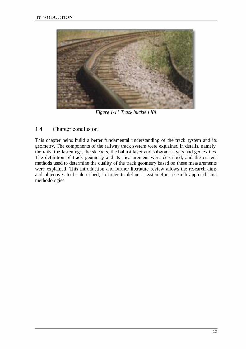
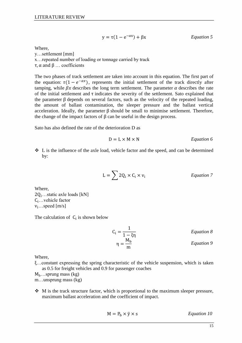
Equation 5
Where,
y…settlement [mm]
x…repeated number of loading or tonnage carried by track
… coefficients
The two phases of track settlement are taken into account in this equation. The first part of
the equation: , represents the initial settlement of the track directly after
tamping, while describes the long term settlement. The parameter describes the rate
of the initial settlement and indicates the severity of the settlement. Sato explained that
the parameter depends on several factors, such as the velocity of the repeated loading,
the amount of ballast contamination, the sleeper pressure and the ballast vertical
acceleration. Ideally, the parameter should be small to minimise settlement. Therefore,
the change of the impact factors of can be useful in the design process.
Sato has also defined the rate of the deterioration D as
Equation 6
L is the influence of the axle load, vehicle factor and the speed, and can be determined
by:
∑ Equation 7
Where,
…static axle loads [kN]
…vehicle factor
…speed [m/s]
The calculation of is shown below
Equation 8
Equation 9
Where,
…constant expressing the spring characteristic of the vehicle suspension, which is taken
as 0.5 for freight vehicles and 0.9 for passenger coaches
…sprung mass (kg)
m…unsprung mass (kg)
M is the track structure factor, which is proportional to the maximum sleeper pressure,
maximum ballast acceleration and the coefficient of impact.
Equation 10
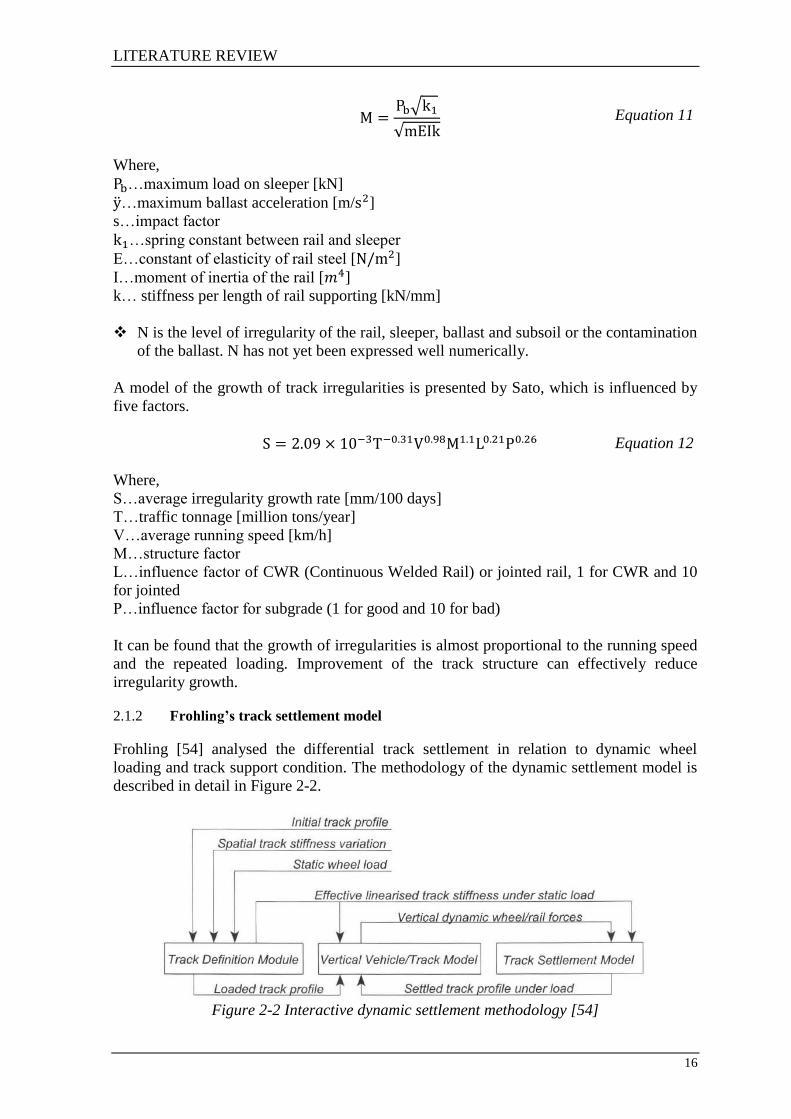
LITERATURE REVIEW
16
√
√ Equation 11
Where,
…maximum load on sleeper [kN]
…maximum ballast acceleration [m/ ]
s…impact factor
…spring constant between rail and sleeper
E…constant of elasticity of rail steel [ ]
I…moment of inertia of the rail [ ]
k… stiffness per length of rail supporting [kN/mm]
N is the level of irregularity of the rail, sleeper, ballast and subsoil or the contamination
of the ballast. N has not yet been expressed well numerically.
A model of the growth of track irregularities is presented by Sato, which is influenced by
five factors.
Equation 12
Where,
S…average irregularity growth rate [mm/100 days]
T…traffic tonnage [million tons/year]
V…average running speed [km/h]
M…structure factor
L…influence factor of CWR (Continuous Welded Rail) or jointed rail, 1 for CWR and 10
for jointed
P…influence factor for subgrade (1 for good and 10 for bad)
It can be found that the growth of irregularities is almost proportional to the running speed
and the repeated loading. Improvement of the track structure can effectively reduce
irregularity growth.
2.1.2 Frohling’s track settlement model
Frohling [54] analysed the differential track settlement in relation to dynamic wheel
loading and track support condition. The methodology of the dynamic settlement model is
described in detail in Figure 2-2.
Figure 2-2 Interactive dynamic settlement methodology [54]

LITERATURE REVIEW
17
The settlement, in mm, after N load alternations is defined in Equation 13.
[[ (
)]
]
Equation 13
Where,
…measured average track stiffness of an individual sleeper, after the consolidation
phase [N/m]
…constant factors
…dynamic wheel load [kN]
…reference wheel load [kN]
N…number of load cycles
w…coefficient of track settlement
The process of the accumulated ballast deterioration can be used to account for a mix of
cyclic loadings at a particular sleeper. However, only ballast settlement is considered, and
no ballast degradation is taken into consideration in this model.
2.1.3 Shenton’s Track Settlement Model
Shenton [52] investigated several major factors related to track degradation, the dynamic
forces, rail irregularities, sleeper spacing, sleeper support, ballast settlement and
substructure. A numerical settlement model was developed to forecast the settlements after
N load cycles:
[ √
] Equation 14
Where,
K…track structure factor, a value of K=1.1 is typical for track in Britain
…equivalent wheelset load [t]
h…lifting value [mm]
The equivalent wheelset load is calculated according to the Equation 15, which considers
the fact that high wheelset loads are dominant in settlement. It ensures a more rational
model for the different axle loads .
√∑
∑
Equation 15
According to Dahlberg [51], Equation 13 can be simplified as
Equation 16
Shenton considers the number of load cycles in the settlement model. The coefficient
and depend on the major factors, and are selected to ensure that the second term
becomes significant only if the number of load cycles, N, is larger than . This model
emphasises the relationship between settlement and number of load cycles.

LITERATURE REVIEW
18
2.1.4 Track settlement study from ORE
According to ORE (Office for Research and Experiments of the International Union of
Railways, UIC) studies by Alva-Hurtado and Selig [55], the ballast strain after N identical
load cycles [mm] can be calculated by Equation 17.
Equation 17
Where,
N…number of load cycles
b…constant, approximately 0.2 for an individual sleeper, and around 0.43 for the track grid
…settlement after the first load cycle [mm]
In the ORE track settlement model [56], the settlement after a certain period of operational
load T is described in Equation 18.
Equation 18
Where,
, … coefficients of settlement depending on the quality of the permanent way
T…period of operation load [t]
Like Sato’s model, this model also consists of two parts: the first part describes the
settlement directly after tamping, and the second part represents the track
settlement coupled with the traffic volume. However, an Australian study by Lonescu et al.
[57] has shown that the ORE settlement model is inaccurate under a large number of load
cycles. The track settlement under a large number of load cycles is stated as:
Equation 19
Where,
b…empirical coefficient
The conclusion of the study is that the trains with high axle loads or high wheel dynamic
forces increase track settlement.
2.1.5 Ford’s track settlement model
One limitation of the ORE model is that there is a precondition of identical loading. Ford
[58] has modified Equation 17 to investigate the varying load cycles. is redefined as
which is a curve against the applied stress and failure stress . A new value for N,
which is , is determined by inverting Equation 17.
*
+
Equation 20
Where,
…initial permanent strain corresponding to the new load
e…the current value of permanent strain

LITERATURE REVIEW
19
Therefore, the ballast settlement is determined from Equation 21.
Equation 21
Unlike Sato’s model, the long-term settlement grows logarithmically. There are some
limitations to this model. Some assumptions in the modelling process are not strictly valid.
The confining stress of the ballast and the ballast failure stress are assumed to be constant,
therefore the ballast strain is assumed constant throughout the ballast layer.
2.1.6 Al Shaer’s settlement study
Al Shaer, Duhamel et al. [59] tried to link the settlement with the acceleration for high load
velocities based on experimental results. A reduced scale (1/3) ballasted railway track is
represented by three sleepers, and these sleepers are loaded with the help of three hydraulic
jacks that provide signals having the shape of the letter M. A moving load is therefore
simulated at different rolling velocities, and the relationship between the load velocity and
the increment of the settlement is shown in Figure 2-3.
Figure 2-3 Relation between velocity and settlement increment [59]
Furthermore, the relationship between increment of the standard deviation caused by the
settlement and the average accelerations of the sleeper in the upward and downward
directions is studied, and a linear relationship is found between them. However, the linear
relationship is only accurate when the speed is below 360 km/h.

LITERATURE REVIEW
20
2.1.7 Gao and Zhai’s track settlement model
Gao and Zhai [60] investigated track settlement by combining the vehicle-track coupling
vibration model and the track settlement model. The dynamic response and the
irregularities of the track are taken as a feedback to the model, as shown in Figure 2-4.
Figure 2-4 Research method of track settlement [60]
The numerical track settlement model is shown in the Equation 22 and Equation 23.
∑
Equation 22
Equation 23
Where,
…track settlement [mm]
…track settlement under i load cycles [mm]
N…number of load cycles
and … experimental coefficient
…ballast acceleration [m/ ]
… ballast stress [ ]
The interaction between vehicle dynamics and dynamic track performance are considered
in the study. Different types of track structure and operational factors can be used as the
input in this model. It is found that the roughness of the surface of the wheel and rail has a
strong impact on track settlement behaviour.
2.1.8 Track vertical deterioration study from BRR (British Rail Research)
In the track deterioration study by BRR [61], the effects of track bed stiffness variation on
track geometry deterioration are identified. A number of basic contributors to track
geometry deterioration have been determined in order to predict:

LITERATURE REVIEW
21
Dynamic forces due to unsprung mass response to weld dips and the resulting track
quality
Dynamic forces due to unsprung mass response to general track roughness and the
resulting track quality
Track quality due to vehicle body response to general track roughness
These three aspects are combined together to calculate the total track SD, and the equation
is shown below.
(
)
(
)
(
)
⁄
Equation 24
However, further equations derived in the track geometry model have not yet been
validated. Additionally, the model was only used to analyse a limited number of test cases
as part of the Eurobalt project.
2.2 Track system models
Track system dynamics has been extensively studied, and various mathematical models
have been developed for design and maintenance purposes. Most track models assume that
the track system is excited by a single wheel or a single bogie with two wheelsets [62]. The
track system is most commonly modelled either in the frequency or the distance domain.
Spatial domain methods use variable frequencies to excite the track at a fixed point along
the track, while distance domain methods use variably moving loads applied along the
track during a certain time period. Most spatial domain track studies are based on the
infinite Euler-Bernoulli and Timoshenko beam models [63, 64]. In general, there are two
methods that simulate the vibration behaviour of the rail, which are the Finite Element
Analysis (FEA) and Vibration Modal method. The vibration modal method effectively
reduces the number of Degrees of Freedom (DOF), and hence, the calculation time, while
the FEA is better at dealing with nonlinear factors in the track system [65]. Track models
are also classified as rails resting on a continuous support or on discrete supports, which
are discussed in detail in [66].
2.2.1 BOEF model
Beam on elastic foundation models (BOEF) are relatively simple track models, in which
the track foundation modulus is based on experimental tests [66, 67]. BOEF can be
considered for track behaviour at rail level, but the track foundation beneath the rail is
oversimplified as a foundation modulus. Therefore, BOEF models are not ideal for track
lateral movement modelling. Figure 2-5 shows an early model that describes the railway
track system, in which the infinite beam is continuously supported by an elastic foundation.
A fourth order partial differential equation (PDE) describes the BOEF model, as shown in
Appendix B. It is a simple model that ignores the dynamic behaviour of the sleepers and
ballast, and the discrete support at the sleepers is also simplified. The model is useful to
understand the basic dynamics of the track system, and can solve some low frequency
dynamic problems.

LITERATURE REVIEW
22
Figure 2-5 Track movement model
2.2.2 Layered elastic models
Based on a BOEF model, layered elastic models [68, 69] can be used, which give a more
realistic dynamic behaviour. Layered elastic models are mainly static track system models,
in which the average modulus of each layer of the track is used, and the pressure
distribution at different track system layers can be found.
Figure 2-6 Double Layer Elastic Track Model
For a double layer elastic model (Figure 2-6), a fourth order PDE can be built for the rail,
and a second order PDE can be established for each track bed layer. For both BOEF and
layered elastic models, the vibrational behaviour of the track can be analysed, however, it
is difficult to add a moving load and non-linear behaviour of the interfaces between
different track subsystems to these models.
Finite Element (FE) models [70, 71] and layered elastic models [68, 69] are both quasi-
static track system models. In layered elastic models, the average modulus of each layer of
the track is used, and the pressure distribution at different track system layers can be found.

LITERATURE REVIEW
23
2.2.3 Discrete supported track model
BOEF and layered elastic models all assume that the rail is continuously supported,
however, in reality, the track is supported discretely. Consequently, discrete supported
models have been developed, as shown in Figure 2-7.
Figure 2-7 Double layer discretely supported track model
Two methods are widely used to describe and solve a discretely supported track model,
which are the Finite Element Analysis and modal analysis. The vibration modal analysis
effectively reduces the number of Degrees of Freedom (DOF), and hence, the computation
time, while the FE model is better at dealing with the nonlinear factors in the track system
[65]. Advanced vehicle dynamics analysis tools exist, such as VAMPIRE®2
and
SIMPACK3 (Website 5). These vehicle dynamics packages can use track geometry data
obtained from a Track Recording Coach (TRC). However, this tool cannot simulate the
loading in the track bed or easily allow representative variations of the vertical and lateral
track stiffness [72]. Furthermore, these software systems do not allow multiple layer track
models and relative force connection between track elements underneath adjacent axles.
2.3 Track lateral irregularity studies
Track lateral stability is a key requirement to ensure safety and passenger comfort. Track
lateral shift and buckling can cause serious running stability problems or even derailment.
Therefore, it is important to identify the mechanism of track lateral movement under
dynamic wheel loads. Lateral displacement resistance plays an essential role in stabilising
the track, and it is mainly influenced by the lateral sleeper support, stress free temperature,
condition of joints, friction between sleeper and ballast, and the effect of tamping [73].
Unlike the vertical displacement, track lateral displacement is affected by vertical, lateral
and longitudinal forces. If the vertical force is high, the resistance between the ballast and
the sleeper is high. Therefore, the L/V load ratio is a critical parameter in track lateral
movement. The longitudinal force can lead to track uplift or exert a lateral misalignment,
shown in Figure 2-8. The black line represents the rail, and the orange line shows the
longitudinal force and the decomposition of this force along the track and perpendicular to
the track.
2 Vampire is copyright 2013 and registered trademark of DeltaRail Group pc. Derby
3 Simpack is copyright 2013 of Simpack AG. Gilching Germany.

LITERATURE REVIEW
24
Figure 2-8 Initial lateral misalignment effected by longitudinal force
There have not been many studies about the development of the track lateral misalignment
by dynamic load cycles. One model was developed in France following track buckling
studies.
2.3.1 Prud’homme studies
One of the earliest studies of track lateral misalignment was undertaken by Prud’homme
[74]. The lateral resistance of wooden sleeper track under a moving lateral load was
experimentally evaluated. The vertical load remained constant while the lateral load
incremented after every Track Loading Vehicle (TLV) pass. The first empirical equation
for the lateral resistance of track with timber sleepers was developed, and is given in
Equation 25.
Equation 25
Where,
…track lateral resistance [kN]
V…vertical axle load [kN]
The Prud’homme limit provides a good guideline to following lateral track movement
studies, but some important factors, such as curvature and rail thermal load effects, were
not considered in this equation. In the following study [75], Equation 25 is improved to
reflect the rail temperature, track curvature, track stiffness and rail profile properties.
Equation 26
[ (
)]
Equation 27
Where,
R… curve radius (m)
T… temperature of the rails above the neutral temperature (C)
…bending rigidity of both rails in the lateral direction ( )
…bending rigidity of both rails in the vertical direction ( )
A… rail cross sectional area ( )
…foundation modulus of the track ( )

LITERATURE REVIEW
25
2.3.2 Kabo’s track lateral resistance studies
After Prud’homme’s study, a three-dimensional FE model [76] was developed to study
ballast resistance under vertical and lateral loading against various influencing factors. The
sleeper is modelled as an elastic body with material properties of concrete, and the ballast
is modelled using an elastoplastic constitutive continuum model of a granular material that
accounts for non-linear hardening and compaction. Four different geometries of ballast
shoulder have been analysed against different vertical loads and friction, and it shows that
either widening the ballast shoulder or increasing the shoulder height can increase the
lateral resistance significantly.
The results show that the peak lateral ballast resistance for a single concrete sleeper varies
from 5 to 18 kN as the ballast compaction increases. The results also show that the
deterioration is not closely related to subgrade stiffness, while the top ballast layer suffers
the most strain and is the leading contributor to the settlement.
2.3.3 Lateral sliding track resistance study at the University of Southampton
The resistance of the railway track is more complex than the lateral resistance defined by
Prud’homme. Three contact areas between the ballast and sleeper, which are the sleeper
base, ballast crib and shoulder, are analysed in a recent experimental study [77] at the
University of Southampton. The sleeper base study is based on an empirical relationship
[78] of normal, lateral and moment loads at failure.
The maximum bearing capacity of the base resistance can be calculated by
Equation 28
In which,
{
Equation 29
Where,
…bearing capacity factor
…analogous to the bearing capacity factor found in the Meyerhof formula [79]
…passive pressure coefficient
…shape factor from Meyerhof formula
…angle of effective shearing resistance [rad]
B…foundation width [m]
L…foundation length [m]
…bulk unit weight of ballast [kN/ ]
u…pore water pressure
The crib resistance can be determined using
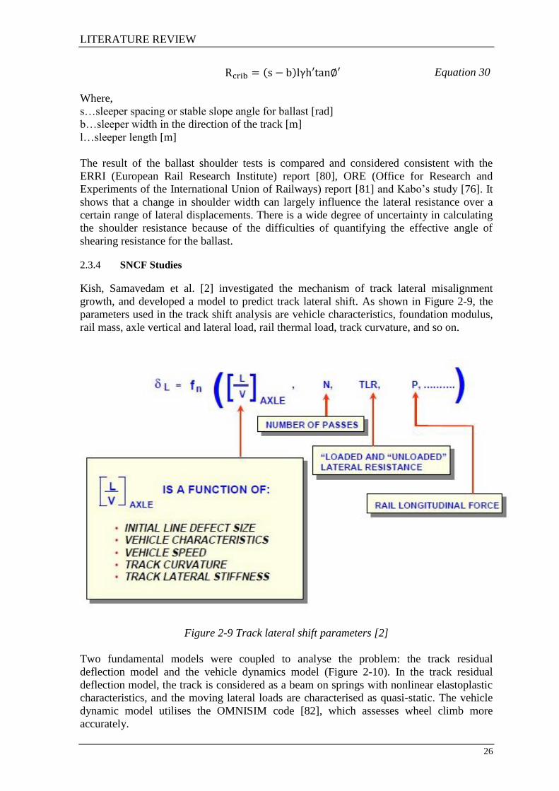
LITERATURE REVIEW
26
Equation 30
Where,
s…sleeper spacing or stable slope angle for ballast [rad]
b…sleeper width in the direction of the track [m]
l…sleeper length [m]
The result of the ballast shoulder tests is compared and considered consistent with the
ERRI (European Rail Research Institute) report [80], ORE (Office for Research and
Experiments of the International Union of Railways) report [81] and Kabo’s study [76]. It
shows that a change in shoulder width can largely influence the lateral resistance over a
certain range of lateral displacements. There is a wide degree of uncertainty in calculating
the shoulder resistance because of the difficulties of quantifying the effective angle of
shearing resistance for the ballast.
2.3.4 SNCF Studies
Kish, Samavedam et al. [2] investigated the mechanism of track lateral misalignment
growth, and developed a model to predict track lateral shift. As shown in Figure 2-9, the
parameters used in the track shift analysis are vehicle characteristics, foundation modulus,
rail mass, axle vertical and lateral load, rail thermal load, track curvature, and so on.
Figure 2-9 Track lateral shift parameters [2]
Two fundamental models were coupled to analyse the problem: the track residual
deflection model and the vehicle dynamics model (Figure 2-10). In the track residual
deflection model, the track is considered as a beam on springs with nonlinear elastoplastic
characteristics, and the moving lateral loads are characterised as quasi-static. The vehicle
dynamic model utilises the OMNISIM code [82], which assesses wheel climb more
accurately.
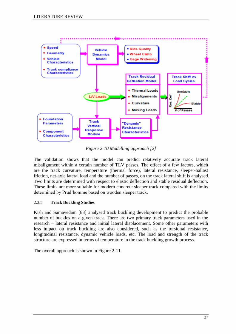
LITERATURE REVIEW
27
Figure 2-10 Modelling approach [2]
The validation shows that the model can predict relatively accurate track lateral
misalignment within a certain number of TLV passes. The effect of a few factors, which
are the track curvature, temperature (thermal force), lateral resistance, sleeper-ballast
friction, net-axle lateral load and the number of passes, on the track lateral shift is analysed.
Two limits are determined with respect to elastic deflection and stable residual deflection.
These limits are more suitable for modern concrete sleeper track compared with the limits
determined by Prud’homme based on wooden sleeper track.
2.3.5 Track Buckling Studies
Kish and Samavedam [83] analysed track buckling development to predict the probable
number of buckles on a given track. There are two primary track parameters used in the
research – lateral resistance and initial lateral displacement. Some other parameters with
less impact on track buckling are also considered, such as the torsional resistance,
longitudinal resistance, dynamic vehicle loads, etc. The load and strength of the track
structure are expressed in terms of temperature in the track buckling growth process.
The overall approach is shown in Figure 2-11.
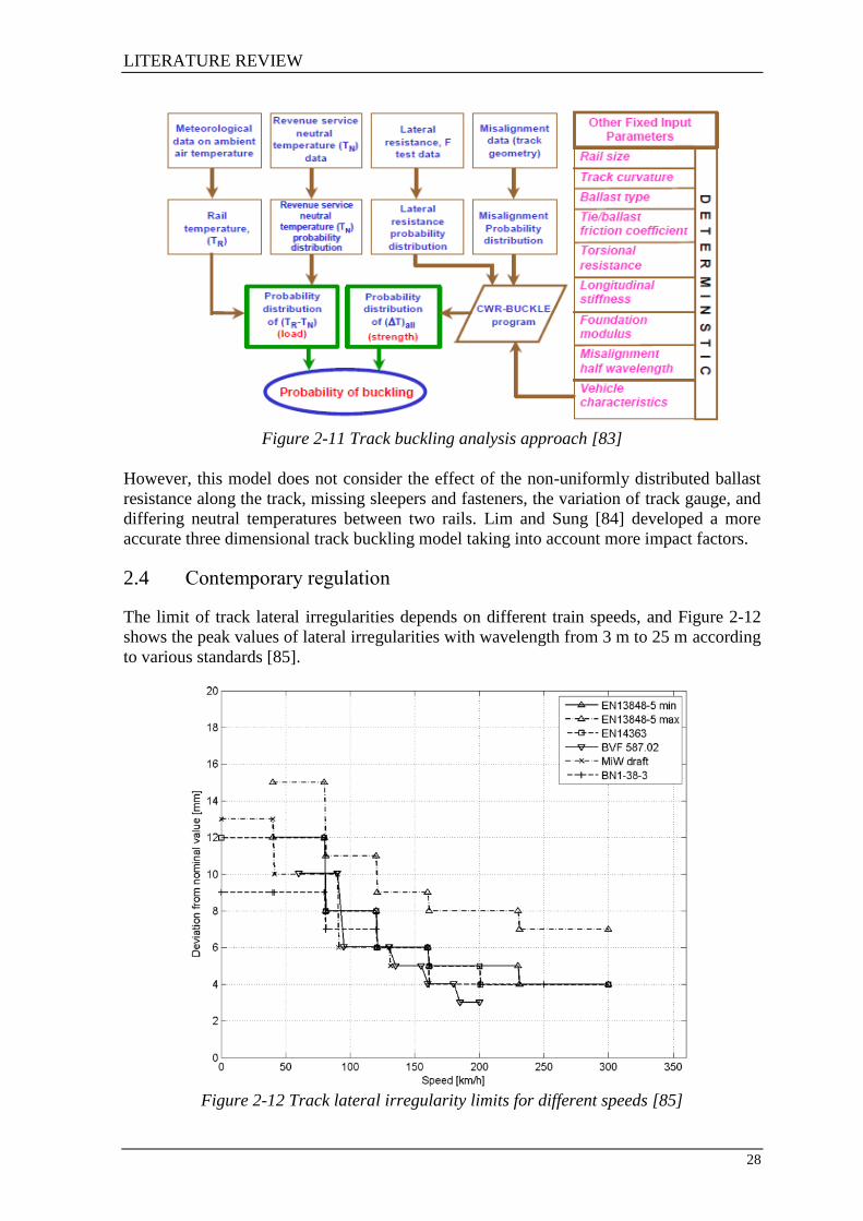
LITERATURE REVIEW
28
Figure 2-11 Track buckling analysis approach [83]
However, this model does not consider the effect of the non-uniformly distributed ballast
resistance along the track, missing sleepers and fasteners, the variation of track gauge, and
differing neutral temperatures between two rails. Lim and Sung [84] developed a more
accurate three dimensional track buckling model taking into account more impact factors.
2.4 Contemporary regulation
The limit of track lateral irregularities depends on different train speeds, and Figure 2-12
shows the peak values of lateral irregularities with wavelength from 3 m to 25 m according
to various standards [85].
Figure 2-12 Track lateral irregularity limits for different speeds [85]

LITERATURE REVIEW
29
Resistance to Lateral Displacement (RLD) is the value of the resistance to lateral track
irregularities which is important in the geometric stability to withstand buckling.
Different forms of the Prud’homme equation are used as a vehicle acceptance criterion in
many countries [86-91]. However, it is considered over simplified to describe the
mechanism of lateral track movement. Additionally, the experiment was based on track
with timber sleeper and lighter rail sections, while the track system and traffic scenario
have significantly changed with the development of the concrete sleepers amongst other
things.
The current SNCF practice on misalignment tolerances and load limits for high-speed
trains is given in a recent SNCF paper [92]. In this paper, the critical misalignment at
which operations are impacted and safety is potentially compromised is indicated as a
12mm peak to peak value with a wavelength range of 20-40m. The maximum allowable
misalignment before maintenance should be smaller. Concrete sleepers on granite ballast
must be designed such that the minimum lateral resistance should be around 13.3-17.8
kN/sleeper.
The current US high speed standard, defined by the Federal Railroad Administration
(FRA), indicates an L/V load ratio of around 0.5 for different values of vertical axle loads.
It gives higher allowable values than given by the Prud’homme limit [93]. Furthermore,
the limit in this study also varies with the change of vertical load, as shown in Table 2-1.
Table 2-1 Proposed net axle L/V limits
V (kN)
L/V limit
L/V=0.28+4.46/V
(no alignment defect)
L/V=0.28+3.97/V
(with alignment defect)
89 0.50 0.48
133 0.43 0.41
178 0.39 0.38
245 0.36 0.35
2.5 Chapter conclusion
It is important to understand the mechanisms behind the development of track irregularities,
and many studies have been carried out to model track vertical irregularities. A comparison
study of different settlement models [94] shows that there are considerable differences
between the models, and it is necessary to consider various parameters in order to choose a
suitable model. Most of the numerical models are empirical and based on duplicate
experiments. However, lateral track misalignment development is not well understood,
because little research has been carried within this area. Contemporary regulations are
mostly based on the Prud’homme limit, which is a simple function with two parts
involving the L/V loading ratio and static lateral resistance. This model may be improved
by considering dynamic influences rather than just the net L/V ratio and lateral forces. A
limit for the size of lateral track irregularities for different speeds is defined, yet without
considering many other influencing factors. All of these limits may not be efficient from
the maintenance point of view, which can be increased by having an accurate prediction of
a particular railway line.

STATISTICAL ANALYSIS OF TRACK QUALITY
30
3 STATISTICAL ANALYSIS OF TRACK QUALITY
This chapter contains a series of statistical analysis studies about the relationship between
lateral and vertical irregularities, between track lateral irregularities and curvature, and
about the track lateral deterioration over time. For the first two relationships, it is better to
have lots of track data covering long sections of different types of track. For track
deterioration over time, it is better to have data covering the same section of track
measured at different time intervals. Therefore, track data from the European project
DynoTrain has been chosen for the first two studies, while the West Coast Main Line
(WCML) and East Coast Main Line (ECML) data sets have been used for studying lateral
track deterioration over time. The standard deviation of track alignment low pass filtered
below 35m wavelength is generally considered to be a good overall indicator of track
quality [95]. Therefore, the irregularity data filtered at 35m is selected in the statistical
analysis.
3.1 The relationship between track lateral and vertical irregularities
In order to obtain representative results, the input data to the statistical analysis should be
representative of a wide range of track conditions. A large amount of track data produced
by the EU project DynoTrain was chosen for this research because it covers track
representative of different countries and different running speeds. This track database
contains measured track data from 6 European railway networks and 3 of them were
selected for this work. Each network database consists of track categories with different
operational speeds shown in Table 3-1. There is a lot of track information with a total
length more than 5800 km.
Table 3-1 Track categories Freight lines
Regional lines
Upgraded lines
High speed lines
There are many more studies into vertical track deterioration than lateral track deterioration.
One of the most important reasons is that the changes in the lateral alignment are slower
than the changes in vertical alignment under typical loading cycles [96]. Therefore, the
maintenance of lateral misalignment is usually considered to be less important. Most track
settlement models only include the vertical influence factors and ignore the lateral
parameters. The deterioration in the lateral direction is a nonlinear phenomenon because of
the highly nonlinear behaviour of vehicles in curves or on straight track due to possible
hunting behaviour, and is related to forces on both vertical and lateral direction. On the
contrary, the vertical settlement of track is very much governed by vertical axle load and
vehicle speed only.
However, as an indivisible load supporting system, it is possible that the track lateral
alignment has an impact on the vertical track settlement behaviour. Reduced horizontal
residual stresses that confine the ballast layer can decrease the stability of the track [97].
Therefore, it is sensible to analyse the relationship between the lateral and vertical track
settlement.

STATISTICAL ANALYSIS OF TRACK QUALITY
31
3.1.1 Distance domain analysis
Firstly, a correlation coefficient is used to see if there is a strong linear relationship
between track lateral and vertical irregularities. For data sets and
, the level of scatter of the data set around the best-fit line can be
measured by the correlation coefficient r, as defined in Equation 31. The detailed linear
regression description is shown in Appendix A.1. The correlation coefficient takes a value
between -1 and 1. The data is completely correlated positively when r equals 1 (-1 means
correlated negatively), while the data is not linearly related at all when r equals 0. There
are three level of correlation: | | shows the data sets are not correlated, | | shows some degree of correlation, and | | indicates a high correlation [98].
∑ ∑ ∑
√ ∑ ∑ √ ∑
∑ Equation 31
The SD values of 200, 600 and 1000 m track irregularities in both vertical and lateral
directions are calculated and are compared. The calculation results are shown in Appendix
A.1., and it is found that results calculated using different track length show similar trends.
Therefore, the typical 200 m SD results are chosen to describe the relationship between
vertical and lateral irregularities in this section.
The correlations between the vertical and lateral irregularity SD results of tangent and
curved track are separately calculated and the coefficients are listed in Table 3-2. For
Network C, the track sections are relatively shorter so the result may not be as accurate as
the results from Network A and B. In order to find more representative results, all track
sections of different types of tracks from all networks are combined together, and the
overall results are shown in the last column in the table. Generally speaking, the correlation
coefficients are bigger than 0.4 which indicates a reasonable relationship between vertical
and lateral irregularities, in the sense that decreasing quality in the vertical direction
generally coincides with decreasing quality in lateral direction.
Table 3-2 Correlation coefficient of track lateral and vertical irregularities Types
Networks
Freight
lines
Regional
lines
Upgraded
lines
High
speed lines
Total
track
Tangent
track
Network A 0.8222 0.5947 0.5690 0.2667
0.4926 Network B - 0.4610 0.4884 0.4779
Network C -0.0688 0.0283 0.2843 -
Curved
track
Network A 0.7280 0.6637 0.6196 0.2722
0.5562 Network B - 0.4630 0.4474 0.3806
Network C 0.2482 -0.0533 0.3565 -
Figure 3-1 shows the linear regression of the overall combined track data results for
tangent and curved track respectively. The pink dashed line represents the limit when
lateral irregularity SD equals the vertical SD. There are a few points with lateral SD bigger
than the lateral limit provided by the standard in Section 2.4. However, the number of these
points are smaller than 4 in both plots, so the influence of these points on the statistical
analysis result can be ignored.

STATISTICAL ANALYSIS OF TRACK QUALITY
32
a) Tangent track b) Curved track
Figure 3-1 Vertical and lateral irregularities SD results of combined track data
The linear regression line in Figure 3-1 shows a slope smaller than 1, which indicates that
the vertical irregularities are generally larger than the lateral irregularities. The percentages
of lateral irregularity SD larger than the vertical SD are listed in Table 3-3.
Table 3-3 Percentage of sections for which the lateral irregularities are larger than the
vertical ones [%] Types
Networks
Freight
lines
Regional
lines
Upgraded
lines
High speed
lines
Total
track
Tangent
track
Network A 14.63 14.58 16.13 55.98
22.52 Network B - 23.02 38.77 30.50
Network C 23.61 11.06 0.98 -
Curved
track
Network A 29.59 22.75 41.55 48.69 `
33.15 Network B - 31.46 87.58 45.89
Network C 52.35 43.2 2.53 -
In order to understand more about the relationship between lateral and vertical
irregularities, the ratio between each section lateral SD and vertical irregularity SD is
calculated using the overall combined track data, and the distributions of these ratios and a
very good generalized extreme value curve fit are shown in Figure 3-2. The mean values of
the lateral to vertical irregularity SD ratios are 0.78 for tangent track and 0.93 for curved
track. From Table 3-3 and Figure 3-2, it can be concluded that track quality in the lateral
direction is generally better than in the vertical direction. On straight track less than 23% of
lateral SDs are bigger than the vertical SDs, but on curved track this proportion increases
to around 33%. From the probability plot and the generalized extreme value curve fit, it
becomes clear that a non-negligible number of sections have a lateral quality significantly
worse than the vertical with a twofold increase for 3% and 5% of all cases for the tangent
and curved track respectively.

STATISTICAL ANALYSIS OF TRACK QUALITY
33
Tangen
t tr
ack
Curv
ed t
rack
Density plot Probability plot
Figure 3-2 Statistical results of lateral to vertical irregularity ratios
3.1.2 Spatial domain analysis
3.1.2.1 Magnitude squared coherence
The formation and development of track irregularities is the result of a number of random
factors. The data recorded by a TRC usually covers a long distance of a route and contains
various frequency ranges. A Power Spectral Density (PSD) method is good at gaining an
understanding of data in the spatial domain. A PSD analysis treats the track alignment data
as a random signal and measures the typical power per unit of frequency in order to
understand the characteristic of the irregularities distributed on the track. Typical
wavelengths will be chosen for further statistical analysis.
Magnitude Squared Coherence (MSC) is the cross coherence of PSD results, which shows
the level of coherence between two sets of data in the spatial domain with the unit of 1/m.
The Welch method is the most commonly used algorithm in track irregularity analysis. In
the calculation process, the length of the segment analysed should be more than twice the
maximum wavelength in order to avoid negligence in the calculation [99]. The maximum
wavelength of the collected data is 35m and the track data is taken every 0.25 meter, so it
is sensible to take between 512 and 4096 points to calculate the PSD. The calculation
segment should be between 0.128 and 1.024km, which is roughly 3.6 to 29.2 times longer
than the longest wavelength. An MSC results in values from 0 to 1. The data is completely
correlated if the MSC value is 1, while there is no coherence between the data sets if the
MSC value is 0. Table 3-4 shows the MSC results for the track data sets used in previous
PSD analysis. The detailed results of the MSC analysis between lateral and vertical track
irregularities are shown in Appendix A.2.

STATISTICAL ANALYSIS OF TRACK QUALITY
34
Table 3-4 MSC results of the track lateral and vertical irregularities
Types
Networks
Freight lines Regional lines Upgraded lines High speed lines
Frequency
(Hz)
Magnitude
Frequency
(Hz)
Magnitude
Frequency
(Hz)
Magnitude Frequency
(Hz)
Magnitude
Network A 0.188 0.0712 0.0313 0.0191 0.250 0.0168 0.254 0.00721 Network B - - 0.328 0.0218 0.258 0.00484 0.152 0.00893 Network C 0.231 0.0250 0.277 0.0235 0.270 0.152 - -
The results show that the maximum magnitudes of the MSC are all less than 0.2, which
indicates weak correlation between vertical and lateral irregularities at different
wavelengths. The peak MSC occurs at different frequencies, and shows no clear regularity
of correlations in major vertical and lateral irregularity wavelength.
3.1.2.2 Line divider fractal analysis
Fractal analysis is used to deal with objects that seem highly chaotic and random, and is
widely used in many area of science [100] such as: complex 1 dimensional lines, 2
dimensional shapes and 3 dimensional objects. Nowadays, the applications of fractal
analysis cover a wide range, such as landscape or coastline complexity [101], heart rate
analysis [102], diagnostic imaging [103], solid studies [104], etc. Railway track
irregularities contain random characteristics, therefore, fractal analysis can be used to
characterise track geometry data and provide unique numerical values that can quantify
geometry signatures [105]. A variety of algorithms are available to calculate the fractal
dimension, counting the line divider, box counting, variogram and triangular prism method
[106]. The divider method, which is also called the yardstick method, is used to analyse the
track irregularities. The length of the rough line measured by each ruler length, , can be
calculated by simply multiplying the number of ruler lengths , n, as shown in Equation 32.
Equation 32
An example of the deviation of a rough line for the computer simulation is shown in Figure
3-3. The closer the ruler length is to the smallest detail of the rough line, the more accurate
the measured length is.
Figure 3-3 Example of rough line deviation pattern
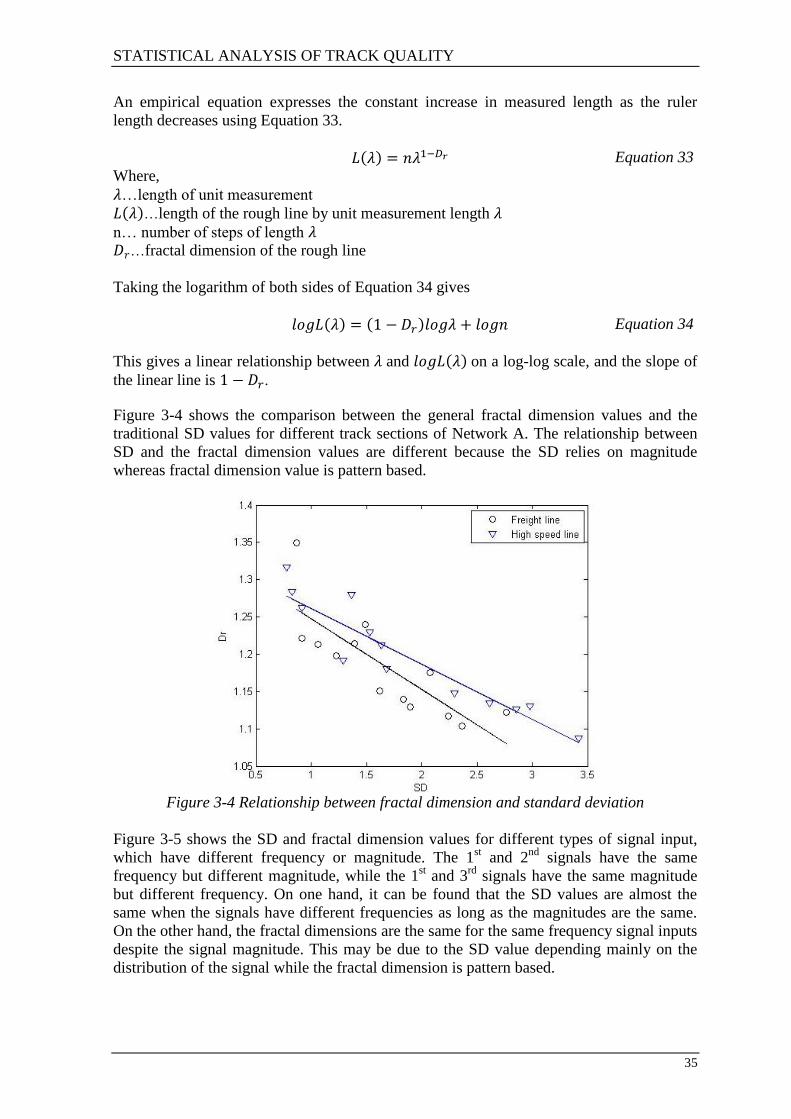
STATISTICAL ANALYSIS OF TRACK QUALITY
35
An empirical equation expresses the constant increase in measured length as the ruler
length decreases using Equation 33.
Equation 33
Where,
…length of unit measurement
…length of the rough line by unit measurement length
n… number of steps of length
…fractal dimension of the rough line
Taking the logarithm of both sides of Equation 34 gives
Equation 34
This gives a linear relationship between and on a log-log scale, and the slope of
the linear line is .
Figure 3-4 shows the comparison between the general fractal dimension values and the
traditional SD values for different track sections of Network A. The relationship between
SD and the fractal dimension values are different because the SD relies on magnitude
whereas fractal dimension value is pattern based.
Figure 3-4 Relationship between fractal dimension and standard deviation
Figure 3-5 shows the SD and fractal dimension values for different types of signal input,
which have different frequency or magnitude. The 1st and 2
nd signals have the same
frequency but different magnitude, while the 1st and 3
rd signals have the same magnitude
but different frequency. On one hand, it can be found that the SD values are almost the
same when the signals have different frequencies as long as the magnitudes are the same.
On the other hand, the fractal dimensions are the same for the same frequency signal inputs
despite the signal magnitude. This may be due to the SD value depending mainly on the
distribution of the signal while the fractal dimension is pattern based.

STATISTICAL ANALYSIS OF TRACK QUALITY
36
Figure 3-5 SD and Dr values for different signal inputs
Therefore, SD is a good tool to evaluate the growth of the irregularity in size while the
fractal dimension is good to analyse the change in irregularity wavelengths. The selection
of the band pass frequency value of the irregularity data has a strong influence on the
fractal dimension value of the track. It is important to use the same band pass processing in
all the original track data sets for a fractal analysis.
The fractal dimensions of each 1km vertical and lateral irregularities were calculated for all
DynoTrain track datasets. All of the calculation results and figures are shown in Appendix
A.4. The correlation coefficient between both vertical and lateral fractal dimensions are
shown in Table 3-5. It was found that the track vertical and lateral irregularities have an
obvious correlation between each other in the spatial domain with correlation coefficient
around 0.4.
Table 3-5 Correlation coefficient of vertical and lateral irregularity fractal dimensions Types
Networks
Freight lines Regional lines Upgraded lines High speed lines
Network A 0.4323 0.3218 0.3984 0.3613
Network B - 0.3854 0.4356 0.3824
Network C 0.1495 0.1678 0.4098 -
3.1.3 Conclusion
Comparing both the distance domain and spatial domain results, it is noted that the vertical
and lateral irregularity magnitudes are clearly correlated with correlation coefficient mostly
bigger than 0.4. However, peak MSC occurs at different frequencies, and shows no clear
regularity of the correlations of the vertical and lateral major irregularity wavelength. In
conclusion, the relationship between vertical and lateral irregularities is obvious in both the
distance domain and spatial domain. The track quality in the vertical direction is generally
worse than in the lateral direction, however some track sections with a lateral quality
significantly worse than the vertical are non-negligible.
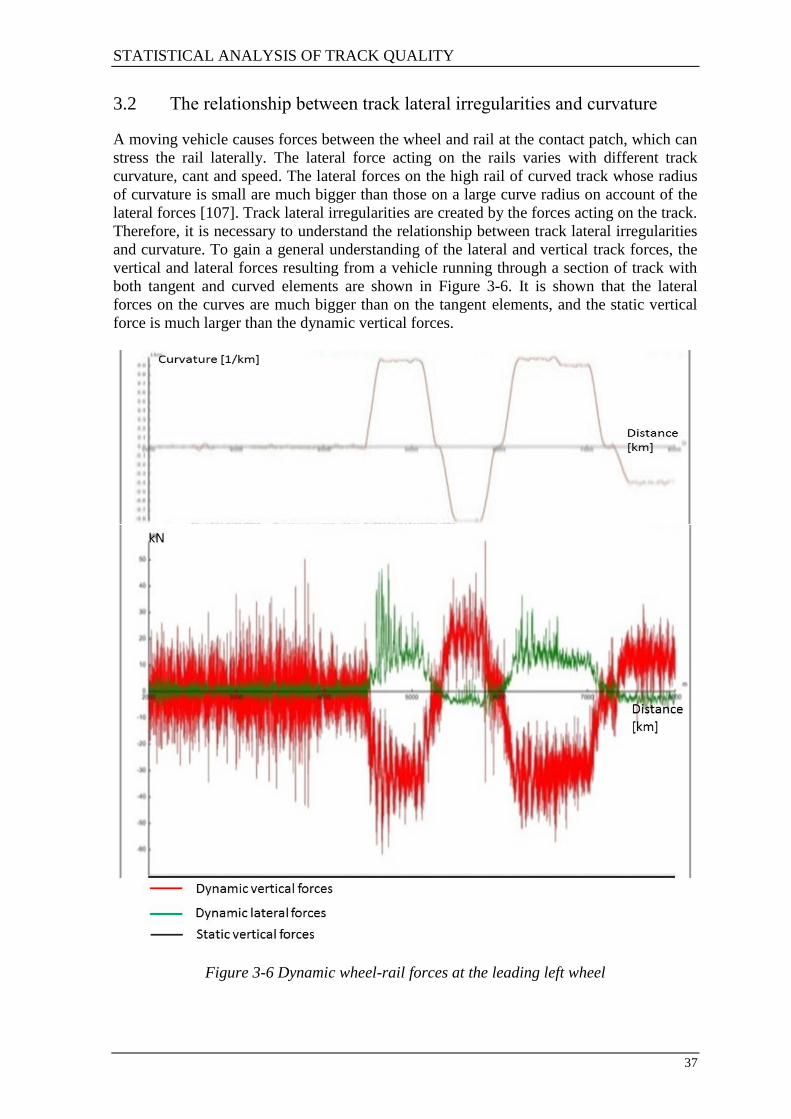
STATISTICAL ANALYSIS OF TRACK QUALITY
37
3.2 The relationship between track lateral irregularities and curvature
A moving vehicle causes forces between the wheel and rail at the contact patch, which can
stress the rail laterally. The lateral force acting on the rails varies with different track
curvature, cant and speed. The lateral forces on the high rail of curved track whose radius
of curvature is small are much bigger than those on a large curve radius on account of the
lateral forces [107]. Track lateral irregularities are created by the forces acting on the track.
Therefore, it is necessary to understand the relationship between track lateral irregularities
and curvature. To gain a general understanding of the lateral and vertical track forces, the
vertical and lateral forces resulting from a vehicle running through a section of track with
both tangent and curved elements are shown in Figure 3-6. It is shown that the lateral
forces on the curves are much bigger than on the tangent elements, and the static vertical
force is much larger than the dynamic vertical forces.
Figure 3-6 Dynamic wheel-rail forces at the leading left wheel

STATISTICAL ANALYSIS OF TRACK QUALITY
38
A MATLAB program written for the EU project DynoTrain is used to select different track
elements, such as tangent track, curved track, switch and crossings, and transitions. For
each network, the curved track sections are selected and divided into six ranges of curve
radius shown in Table 3-6 and the tangent track elements are also selected. The value of
these curve ranges of all data from four networks and different types of lines are box
plotted in Figure 3-7. The box plotting results for each type of line on each network are
also shown in Appendix A.3. The width of the box is defined by Interquartile Range (IQR),
that is, IQR=Q3-Q1, where Q1 and Q3 are the lower quartile and upper quartile. The box
contains 50% of the total values. The red line in the box is the median value of the data, or
50th
percentile, or Q2. An outliner is any value that lays more than 1.5 times the length of
the box from either end of the box. The red points represent the whisker outliers in the data
sample, which are defined if they are larger than the greatest value: Q3+1.5IQR or smaller
than least value: Q1-1.5IQR.
a) Box plot result
b) Cumulative probability result
Figure 3-7 SD value against different curve radius ranges

STATISTICAL ANALYSIS OF TRACK QUALITY
39
The figures show that there is a clear trend towards a worsening lateral track quality as the
curves get sharper. This result can be quite representative because it contains a
comprehensive amount of track data, equivalent to 4545.3km of track, including freight,
original, upgraded and high speed lines. A clear trend can be found that the track quality
deteriorates as curve radius reduces. The median values of SD for all of the curvature
ranges are shown in Table 3-6.
Table 3-6 Median SD value in different curvature range
1 2 3 4 5 6 7
Curve radius
range [1/km]
0-0.2 0.2-
0.5751
0.5751-
1.1501
1.1501-
1.7253
1.7253-
2.3004
2.3004-
2.8752
2.8752-
3.4506
Curve radius
range [m]
Straight
line
5000-
1739
870-
1739
580-
870
435-
580
348-
435
290-
348
Median SD
[mm]
0.9974 1.0760 1.4192 1.8590 2.0566 4.1725 6.5404
[mm] 0 0.0786 0.4218 0.8616 1.0592 3.1751 5.543
By plotting the values, which are the differences between the median SD values, an
exponential growth characteristic can be found, as shown in Figure 3-8.
Figure 3-8 Median SD growth plotting against different curvature ranges
Two different types of curve fitting were applied to the median lateral irregularity SD
value against the curve radius range. The exponential curve gives a better fit to the
data than the equation, while an power curve gives a better fit
than . So the exponential equation and the power curve equation
results are shown in Table 3-7. The best curve fitting result using data set 2 with a power
curve fitting equation is shown in Figure 3-9. A Sum of Squared Errors of prediction (SSE),
, adjusted and a Root Mean Squared Errors (RMSE) are all measures of the
discrepancy between the data and the estimation model. A small SSE and RMSE value
indicates a close correlation between the curve fitting equation and the data, while the
closer and adjusted are to 1 the better the curve fits the data. Data set 1 and 2
represents the whole set of data, and data without the curve range number 4.

STATISTICAL ANALYSIS OF TRACK QUALITY
40
Table 3-7 Curve fitting results Exponential Power
Data set 1 Data set 2 Data set 1 Data set 2
a=0.09719
b=1.176
a=0.1414
b=1.066
a=0.05761
b=3.662
c=0.2101
a=0.1269
b=3.023
c=0.1494
SSE 0.2923 0.06317 0.2655 0.02293
0.9868 0.9971 0.988 0.9989
Adjust 0.9835 0.9962 0.98 0.9979
RMSE 0.2703 0.143 0.2975 0.1071
Although data set 2 gives a more accurate curve fitting result as shown in Figure 3-9, there
is no strong evidence that indicates curve range number 4 is a bad sample. Meanwhile, the
shaper the curvature is, the less data points will be in the curve range. Therefore, it would
be sensible to collect more data that suffcient in all curve ranges to provide a more accurate
curve fitting result.
Figure 3-9 Best curve fitting result
In conclusion, the lateral forces are directed in both directions on tangent track which
counteract each other, while there is always a large static vertical force due to the vehicle
weight. This explains why the deterioration of railway track in the vertical direction is
greater than in the lateral direction. On curves, railway track tends to deteriorate faster due
to the larger lateral forces as a result of vehicle running with cant deficiency or cant excess.
The track irregularity SD generally tends to show an exponential growth with decreasing
curve radius when considering all track types. This power exponential characteristic may
vary when considering a particular type of railway line, such as freight lines, regional lines
and high speed lines.
3.3 Track lateral deterioration over time
The track data used in this section was recorded by Network Rail over a time interval of 1
to 3 months between Wolverton and Rugby on the West Coast Main Line which has a line
speed of 125mph. The total length of this data set is 7 miles, and contains 6 elements of
curved track and 2 elements of tangent track. All of the curves are numbered and their
radius shown beneath Figure 3-10.

STATISTICAL ANALYSIS OF TRACK QUALITY
41
R =2 km, R =1.05 km, R =1.21 km, R =1.08 km, R =-2.56 km, R =2.78 km
Figure 3-10 Curve profile
The dates that the track data was recorded is shown in Table 3-8.
Table 3-8 Track recording dates and dataset numbers
Date set Date Period between two
measurement dates
(Day) D1 14/04/2010
D2 09/06/2010 56
D3 14/07/2010 35
D4 11/08/2010 28
D5 13/10/2010 63
D6 08/12/2010 56
D7 19/01/2011 42
D8 16/03/2011 56
D9 18/05/2011 63
D10 15/06/2011 28
D11 20/07/2011 35
D12 17/08/2011 28
D13 14/09/2011 28
D14 16/11/2011 63
D15 18/01/2012 63
D16 15/02/2012 28
D17 18/04/2012 63
D18 18/07/2012 91
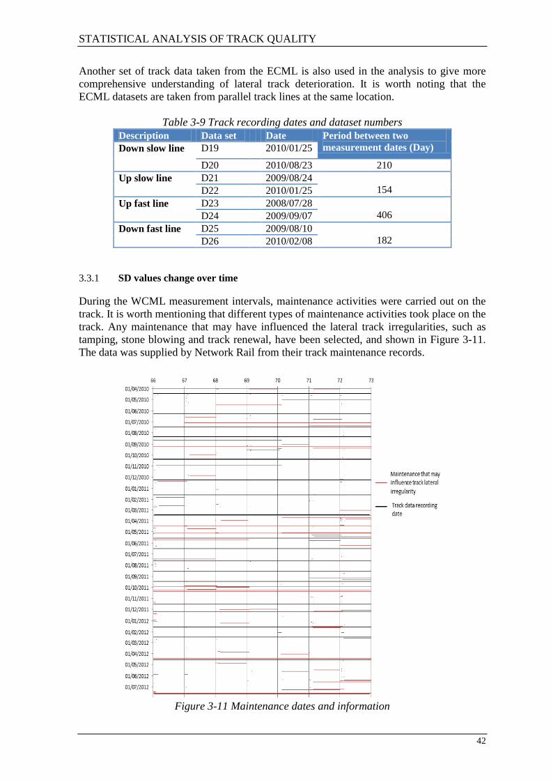
STATISTICAL ANALYSIS OF TRACK QUALITY
42
Another set of track data taken from the ECML is also used in the analysis to give more
comprehensive understanding of lateral track deterioration. It is worth noting that the
ECML datasets are taken from parallel track lines at the same location.
Table 3-9 Track recording dates and dataset numbers
Description Data set Date Period between two
measurement dates (Day) Down slow line D19 2010/01/25
D20 2010/08/23 210
Up slow line D21 2009/08/24
154 D22 2010/01/25
Up fast line D23 2008/07/28
406 D24 2009/09/07
Down fast line D25 2009/08/10
182 D26 2010/02/08
3.3.1 SD values change over time
During the WCML measurement intervals, maintenance activities were carried out on the
track. It is worth mentioning that different types of maintenance activities took place on the
track. Any maintenance that may have influenced the lateral track irregularities, such as
tamping, stone blowing and track renewal, have been selected, and shown in Figure 3-11.
The data was supplied by Network Rail from their track maintenance records.
Figure 3-11 Maintenance dates and information

STATISTICAL ANALYSIS OF TRACK QUALITY
43
Due to the fact that the lateral forces between the vehicle and track occur in both directions,
it is difficult for the track to develop a constantly increasing track lateral deterioration. In
addition, the influence of maintenance on the track cannot be ignored. Consequently, it is
hard to find track sections with growing irregularities. The length of track for the SD value
calculation also has a strong influence on the results. SD values of 30m, 50m, 60m, 90m,
100m and 200m long track sections are used to discover track sections with increasing
lateral irregularities. The location of these sections is shown in Figure 3-12. It can be found
that different measurement lengths lead to quite different locations of the track sections. In
order to get more accurate results, it is sensible to select the overlapped locations of track
sections for the following study.
Figure 3-12 Locations of track sections with reasonable lateral deterioration
Taking the track model into consideration, the length for the calculation of SD values is
chosen to be 60m for the convenience of calculation due to the 0.6m sleeper spacing used
in the track model. Consequently, 18 track sections are selected with at least 6 sets of
recorded track data showing an increasing SD.
Table 3-10 Selected track sections
Track
sections
Location of selected
sections [m]
Lateral irregularity
increasing data sets
Curvature of selected
section [mm]
S1 540 -600 D2-D8 0
S2 660-720 D9-D14 0
S3 720-780 D9-D14 0
S4 1800-1860 D8-D13 0
S5 1980-2040 D10-D15 0
S6 2400-2460 D7-D13 0

STATISTICAL ANALYSIS OF TRACK QUALITY
44
S7 3240-3300 D6-D12 0
S8 4140-5200 D6-D12 0
S9 7320-7380 D8-D13 Transition to
S10 7860-7920 D8-D14
S11 7920-7980 D8-D13
S12 9840-9900 D3-D13
S13 10200-10260 D8-D13 Transition to
S14 10260-10320 D8-D13 Transition to
S15 10380-10440 D8-D14 0
S16 10440-10500 D8-D13 0
S17 10500-10560 D8-D14 0
S18 10800-10860 D8-D13 0
Among the maintenance activities, tamping and stone blowing have the largest influence
on lateral geometry correction. Therefore, they are selected to be considered in the research.
The dates that these two maintenance activities were undertaken and the track sections
with increasing lateral deterioration are shown in Figure 3-13. It can be found that most of
the selected track sections are not influenced by tamping or stone blowing. The sections
that were influenced by maintenance activities are not considered in the following research.
Figure 3-13 Tamping and stone blowing maintenance activities

STATISTICAL ANALYSIS OF TRACK QUALITY
45
The final selected datasets for the lateral deterioration analysis are shown in Table 3-11.
Table 3-11 Selected lateral deterioration data sets
60m SD
S1 S2 S3 S4 S5 S6 S7 S8 S9
66.336 66.41 66.448 67.119 67.23 67.491 68.013 68.573 70.549
14/04/2010
09/06/2010 0.8196
14/07/2010 1.0145
11/08/2010 1.1661
13/10/2010 1.2874
08/12/2010 1.5481
19/01/2011
16/03/2011
1.3357
18/05/2011
0.5036 0.8921 0.2721
0.296 0.7742 1.2145 1.3968
15/06/2011
0.5149 0.9457 0.3267 0.3899 0.3067 0.8252 1.2657 1.5348
20/07/2011
0.562 1.0645 0.3479 0.4267 0.3338 0.8665 1.2812 1.5924
17/08/2011
0.8396 1.1292 0.3611 0.4347 0.3376 0.8823 1.4363 2.0135
14/09/2011
0.987 1.3707 0.4156 0.5232 0.343
2.4245
16/11/2011
1.265 1.5636
18/01/2012
15/02/2012
18/04/2012
18/07/2012
S10 S11 S12 S13 S14 S15 S16 S17 S18
70.884 70.921 72.114 72.338 72.375 72.45 72.487 72.525 72.711
14/04/2010
09/06/2010
14/07/2010
11/08/2010
13/10/2010
08/12/2010
19/01/2011
16/03/2011 1.2907 0.4005 0.7819 0.4605 0.4108 0.2446 0.3245 0.3656 0.3196
18/05/2011 1.4154 0.4197 0.8983 0.5361 0.4211 0.2983 0.3452 0.4213 0.421
15/06/2011 1.516 0.4406 0.9053 0.6105 0.4218 0.2991 0.3693 0.4702 0.5307
20/07/2011 1.7194 0.4514 0.9325 0.8278 0.5808 0.4274 0.4703 0.4754 0.5489
17/08/2011 2.9094 0.5302 1.2207 1.0183 0.8846 0.7259 0.5566 0.5728 0.7704
14/09/2011 3.4214 1.2578 1.3932 1.4992 1.0832 0.8659 0.6143 0.7387 0.921
16/11/2011 3.4298
0.9337
1.1549
18/01/2012
15/02/2012
18/04/2012
18/07/2012
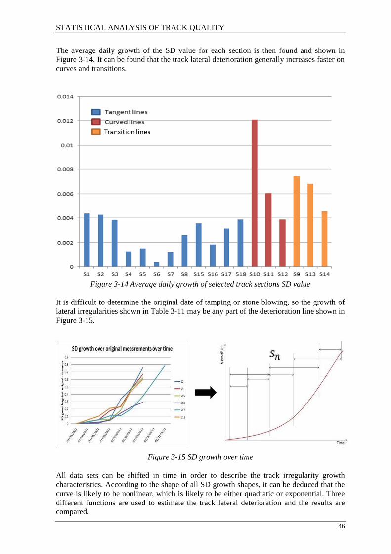
STATISTICAL ANALYSIS OF TRACK QUALITY
46
The average daily growth of the SD value for each section is then found and shown in
Figure 3-14. It can be found that the track lateral deterioration generally increases faster on
curves and transitions.
Figure 3-14 Average daily growth of selected track sections SD value
It is difficult to determine the original date of tamping or stone blowing, so the growth of
lateral irregularities shown in Table 3-11 may be any part of the deterioration line shown in
Figure 3-15.
Figure 3-15 SD growth over time
All data sets can be shifted in time in order to describe the track irregularity growth
characteristics. According to the shape of all SD growth shapes, it can be deduced that the
curve is likely to be nonlinear, which is likely to be either quadratic or exponential. Three
different functions are used to estimate the track lateral deterioration and the results are
compared.

STATISTICAL ANALYSIS OF TRACK QUALITY
47
3.3.1.1 Quadratic function
The estimation function is assumed to be
Equation 35
Where,
…SD growth [mm]
t…time [days]
a,b…parameters
The estimated quadratic curve fitting results for tangent, curved and transition elements are
shown in Table 3-12.
For track consisting mainly of straight track, parameter a is the smallest at roughly
which indicates a small slope and slower lateral deterioration, while for
curved and transition track it is around .
Table 3-12 Curve fitting parameters and evaluations for three types of track sections
a b RMSE
Tan
gen
t tr
ack
est
imat
ion
2.91E-6 9.05E-5 0.0801
Curv
ed t
rack
est
imat
ion
6.87E-6 -6.3E-5 0.2899
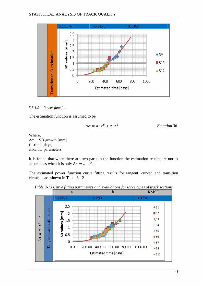
STATISTICAL ANALYSIS OF TRACK QUALITY
48
Tra
nsi
tion
tra
ck e
stim
atio
n
5.53E-6 -6.3E-5 0.1465
3.3.1.2 Power function
The estimation function is assumed to be
Equation 36
Where,
…SD growth [mm]
t…time [days]
a,b,c,d…parameters
It is found that when there are two parts in the function the estimation results are not as
accurate as when it is only .
The estimated power function curve fitting results for tangent, curved and transition
elements are shown in Table 3-12.
Table 3-13 Curve fitting parameters and evaluations for three types of track sections
a b RMSE
Tan
gen
t tr
ack
est
imat
ion
5.22E-7 2.283 0.0796
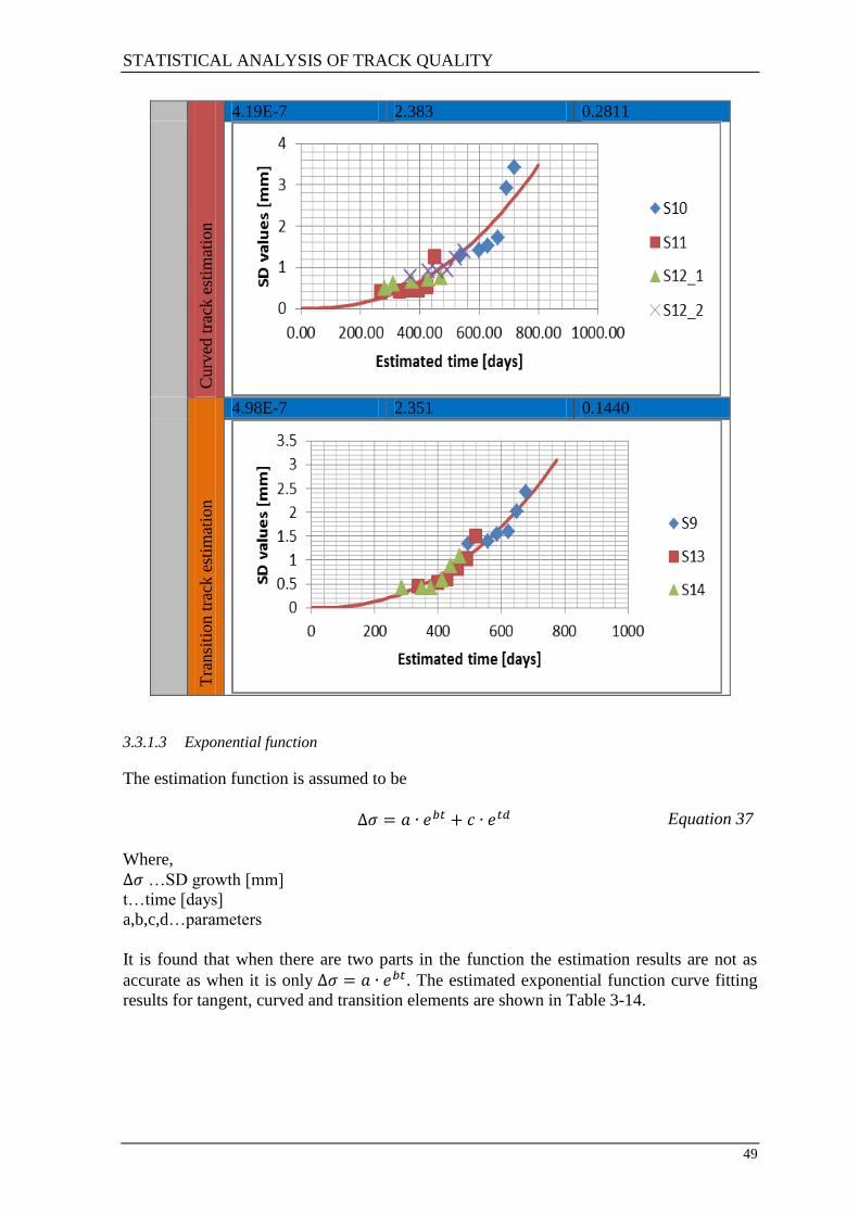
STATISTICAL ANALYSIS OF TRACK QUALITY
49
Curv
ed t
rack
est
imat
ion
4.19E-7 2.383 0.2811
Tra
nsi
tion t
rack
est
imat
ion
4.98E-7 2.351 0.1440
3.3.1.3 Exponential function
The estimation function is assumed to be
Equation 37
Where,
…SD growth [mm]
t…time [days]
a,b,c,d…parameters
It is found that when there are two parts in the function the estimation results are not as
accurate as when it is only . The estimated exponential function curve fitting
results for tangent, curved and transition elements are shown in Table 3-14.

STATISTICAL ANALYSIS OF TRACK QUALITY
50
Table 3-14 Curve fitting parameters and evaluations for three types of track sections
a b RMSE
Tan
gen
t tr
ack
est
imat
ion
0.1159 0.0040 0.0811
Curv
ed t
rack
est
imat
ion
0.084 0.00618 0.2811
Tra
nsi
tion t
rack
est
imat
ion
0.012 0.004857 0.1515
Between the quadratic, power and exponential functions, the power function provides the
most accurate fit to lateral deterioration.
3.3.2 PSD values change over time
The PSD presents an understanding of the track in the spatial domain. It can be found in
Chapter 3.3.1 that datasets D8 to D13 from the WCML are least influenced by
maintenance activities. Therefore, D8 to D13 from the WCML and D19 to D26 from the
ECML were used for the PSD analysis; this is to exclude measurements which have been
influenced by maintenance. The analysis is undertaken in two parts, a long wavelength
analysis and a short wavelength analysis.

STATISTICAL ANALYSIS OF TRACK QUALITY
51
3.3.2.1 Long wavelength analysis
In terms of long wavelength, a linear scale of the PSD on both the x and y axis gives a
better representation of the data. Figure 3-16 shows the long wavelength PSD results for
the D8 to D13 datasets from the WCML and D19 to D26 datasets for the ECML. It can be
seen that the power density is more clearly shown when the wavelength is longer than 10m
in spatial frequency 0.1 cycle/m; therefore, the long wavelength analysis is defined in the
range between 10 to 35 m.
Figure 3-16 PSD result of long wavelength track irregularities

STATISTICAL ANALYSIS OF TRACK QUALITY
52
The peak power density points in the figures are summarised from Figure 3-16 in Table
3-15. It can be found that the peak power densities occur within the spatial frequency range
from 0.03418 to 0.03906 cycle/m which is equivalent to a wavelength of 25.6 to 29.2 m.
Moreover, it is notable that many long wavelength irregularities grow only in size, not
wavelength. Generally, the growth of the irregularity size is quite small and the growth
rates of the power density of these defects are different for different track sections. The
average growth of peak power density per month is around 7-16% of the original power
density.
Table 3-15 Summaries of the long wavelength PSD results
Per
iod
bet
wee
n d
ata
sets
[d
ays]
Dat
a ta
ken
tim
e
[yy
/mm
/dd
]
Pea
k p
ow
er d
ensi
ty
[mm
2/c
ycl
e/m
]
Av
erag
e g
row
th o
f p
eak p
ow
er
den
sity
[m
m2
/cy
cle/
m/m
on
th]
Sp
atia
l fr
equ
ency
at
pea
k
[cy
cle/
m]
Av
erag
e g
row
th o
f ir
regu
lari
ty
wav
elen
gth
[m
m/m
on
th]
Fre
qu
ency
fo
r li
ne
spee
d o
f
12
5m
ph
[H
z]
Per
cen
tag
e o
f d
ecre
ase
of
freq
uen
cy [
%]
1st p
eak
po
wer
den
sity
D8
63
28
35
28
28
16/03/2011 10.150
1.6071
0.03418
0
1.9100
0
D9 18/05/2011 13.020 0.03418 1.9100
D10 15/06/2011 12.500 0.03174 1.7736
D11 20/07/2011 12.540 0.03174 1.7736
D12 17/08/2011 17.090 0.03174 1.7736
D13 14/09/2011 19.900 0.03418 1.9100
D19
210
2010/01/25 16.020 0.1886 0.03906 0
2.1827 0
D20 2010/08/23 17.340 0.03906 2.1827
D21
154
2009/08/24 28.490 0.624 0.03662 389.88
2.0463 6.66
D22 2010/01/25 31.610 0.03418 1.9100
D23
406
2008/07/28 26.670 0.2446
0.03418 0
1.9100 0
D24 2009/09/07 23.490 0.03418 1.9100
D25
182
2009/08/10 7.879 0.2835 0.03906 609.21 2.1827 12.49
D26 2010/02/08 9.580 0.03418 1.9100
2n
d p
eak
po
wer
den
sity
D8
63
28
35
28
28
16/03/2011 8.469
1.1886
0.03906
-0.4022
2.1827
-6.25
D9 18/05/2011 8.519 0.04395 2.4559
D10 15/06/2011 7.480 0.04395 2.4559
D11 20/07/2011 7.667 0.04150 2.3190
D12 17/08/2011 12.180 0.04150 2.3190
D13 14/09/2011 15.680 0.04150 2.3190
D19 210 2010/01/25 11.310 0.2271
0.05371 265.82
3.0013 9.09
D20 2010/08/23 12.900 0.04883 2.7286
D21 154 2009/08/24 25.640 0.3020
0.04639 0
2.5923 0
D22 2010/01/25 27.150 0.04639 2.5923
D23 406 2008/07/28 6.454 0.2445
0.05127 0
2.8649 0
D24 2009/09/07 9.633 0.05127 2.8649
D25 182 2009/08/10 9.601 -0.2330
0.05371 0
3.0013 0
D26 2010/02/08 8.203 0.05371 3.0013
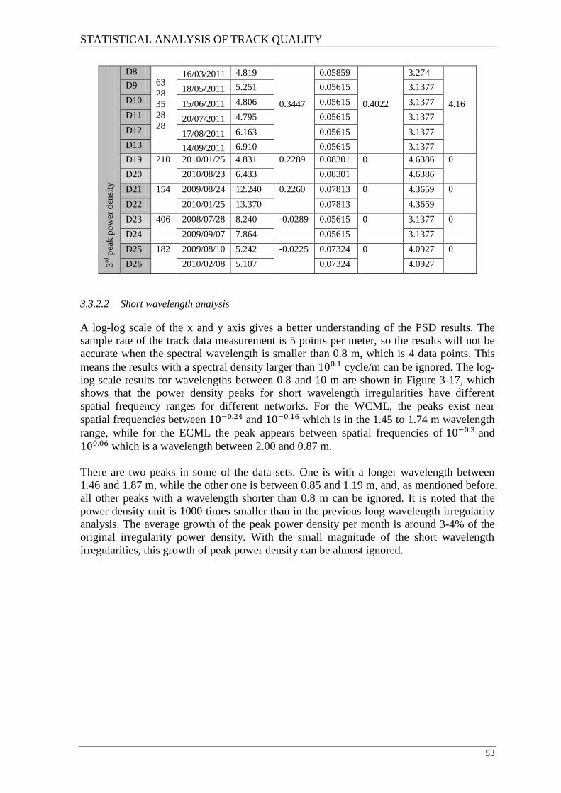
STATISTICAL ANALYSIS OF TRACK QUALITY
53
3rd
pea
k p
ow
er d
ensi
ty
D8
63
28
35
28
28
16/03/2011 4.819
0.3447
0.05859
0.4022
3.274
4.16
D9 18/05/2011 5.251 0.05615 3.1377
D10 15/06/2011 4.806 0.05615 3.1377
D11 20/07/2011 4.795 0.05615 3.1377
D12 17/08/2011 6.163 0.05615 3.1377
D13 14/09/2011 6.910 0.05615 3.1377
D19 210 2010/01/25 4.831 0.2289
0.08301 0
4.6386 0
D20 2010/08/23 6.433 0.08301 4.6386
D21 154 2009/08/24 12.240 0.2260
0.07813 0
4.3659 0
D22 2010/01/25 13.370 0.07813 4.3659
D23 406 2008/07/28 8.240 -0.0289
0.05615 0
3.1377 0
D24 2009/09/07 7.864 0.05615 3.1377
D25 182 2009/08/10 5.242 -0.0225 0.07324 0 4.0927 0
D26 2010/02/08 5.107 0.07324 4.0927
3.3.2.2 Short wavelength analysis
A log-log scale of the x and y axis gives a better understanding of the PSD results. The
sample rate of the track data measurement is 5 points per meter, so the results will not be
accurate when the spectral wavelength is smaller than 0.8 m, which is 4 data points. This
means the results with a spectral density larger than cycle/m can be ignored. The log-
log scale results for wavelengths between 0.8 and 10 m are shown in Figure 3-17, which
shows that the power density peaks for short wavelength irregularities have different
spatial frequency ranges for different networks. For the WCML, the peaks exist near
spatial frequencies between and which is in the 1.45 to 1.74 m wavelength
range, while for the ECML the peak appears between spatial frequencies of and
which is a wavelength between 2.00 and 0.87 m.
There are two peaks in some of the data sets. One is with a longer wavelength between
1.46 and 1.87 m, while the other one is between 0.85 and 1.19 m, and, as mentioned before,
all other peaks with a wavelength shorter than 0.8 m can be ignored. It is noted that the
power density unit is 1000 times smaller than in the previous long wavelength irregularity
analysis. The average growth of the peak power density per month is around 3-4% of the
original irregularity power density. With the small magnitude of the short wavelength
irregularities, this growth of peak power density can be almost ignored.

STATISTICAL ANALYSIS OF TRACK QUALITY
54
Figure 3-17 PSD results of short wavelength track irregularities

STATISTICAL ANALYSIS OF TRACK QUALITY
55
Table 3-16 Summarise of short wavelength PSD results
Per
iod
bet
wee
n d
ata
sets
[d
ays]
Dat
a ta
ken
tim
e
[yy
/mm
/dd
]
Pea
k p
ow
er d
ensi
ty
[mm
2/c
ycl
e/m
m]
Av
erag
e g
row
th o
f p
eak p
ow
er
den
sity
[m
m2
/cy
cle/
mm
/mo
nth
]
Sp
atia
l fr
equ
ency
at
pea
k
[cy
cle/
m]
Av
erag
e g
row
th o
f ir
regu
lari
ty
wav
elen
gth
[m
m/m
on
th]
Fre
qu
ency
fo
r li
ne
spee
d o
f
12
5m
ph
[H
z]
Per
cen
tag
e o
f d
ecre
ase
of
freq
uen
cy [
%]
Sp
atia
l fr
equ
ency
D8
63
28
35
28
28
16/03/2011 1.9000
-
0.0887
0.6006
-1.6154
33.562
-1.63
D9 18/05/2011 0.4997 0.6152 34.377
D10 15/06/2011 0.8085 0.6006 33.562
D11 20/07/2011 1.8960 0.6055 33.835
D12 17/08/2011 0.6336 0.6104 34.109
D13 14/09/2011 1.3600 0.6104 34.109
D19 210 2010/01/25 29.4600 0.4057 0.5664 8.9930 31.650 3.44
D20 2020/08/23 32.3000 0.5469 30.561
D21 154 2009/08/24 - - - - -
D22 2010/01/25 - - -
D23 406 2008/07/28 16.3900 0.0223 0.5859 2.2102 32.740 1.66
D24 2009/09/07 16.6800 0.5762 32.198
D25 182 2009/08/10 37.9600 14.256
7
0.5859 25.8458 32.740 8.33
D26 2010/02/08 123.5000 0.5371 30.013
S
pat
ial
freq
uen
cy
D8
63
28
35
28
28
16/03/2011 1.6670
-
0.0641
0.6641
-0.7912
37.11
-0. 72
D9 18/05/2011 0.3908 0.6836 38.2
D10 15/06/2011 0.8024 0.6592 36.836
D11 20/07/2011 1.6350 0.6787 37.926
D12 17/08/2011 2.2370 0.6689 37.378
D13 14/09/2011 1.2780 0.6689 37.378
D19 210 2010/01/25 8.9570 -
0.6223
1.123 7.0540
62.753 5.25
D20 2020/08/23 4.6010 1.064 59.456
D21 154 2009/08/24 9.7370 1.7066
1.055 26.0135
58.953 12.07
D22 2010/01/25 18.2700 0.9277 51.840
D23 406 2008/07/28 2.2850 0.1258
1.1720 1.1395
65.491 1.71
D24 2009/09/07 3.9210 1.1520 64.374
D25 182 2009/08/10 13.0000 3.6283 1.1820 14.1792 66.050 9.14
D26 2010/02/08 34.7700 1.0740 60.015

STATISTICAL ANALYSIS OF TRACK QUALITY
56
3.3.2.3 Comparison between long and short wavelength PSD results
Figure 3-18 summarises the average growth of peak power density results from Table 3-15
and Table 3-16. The shorter the irregularity wavelength is, the slower the power density
growth. When the irregularity wavelength is below a certain length, the growth of
irregularity size can be neglected. However, from a growth rate point of view, short
wavelength lateral irregularities grow much faster than long wavelength ones.
Figure 3-18 Summary of average peak power density growth per month
Figure 3-19 shows a summary of the irregularity wavelength growth results from Table
3-15 and Table 3-16. A conclusion can be made that most track irregularities grow in
length, but the long wavelength irregularities appear to be more stable than the short ones,
as it can be seen in the figure that many of the long wavelength irregularities settles and the
wave length does not change. The growth of irregularities does not follow a set pattern for
all data sets regardless of size or length, which may be due to different subgrade conditions,
traffic mix and types of track subsystems. However, a specific section of track can be
studied in order to find the pattern of irregularity growth.
Figure 3-19 Summary of growth of irregularity wavelength per month

STATISTICAL ANALYSIS OF TRACK QUALITY
57
3.3.3 Fractal dimensions change over time
Unlike a PSD analysis, an FD analysis does not require a long length of track section to get
enough information. As discussed in section 3.1.2.2, fractal dimension and SD can both
describe the lateral track quality yet in different ways. The overall fractal dimension and
SD are calculated for a section of track, and shown in Figure 3-20.
Figure 3-20 Fractal dimension and SD value change over time
The fractal dimension has a general trend of dropping over time, which describes the
irregularity wavelength growth. However, although the fractal dimension describes the
overall frequency change to some extent, it is easily influenced by the length of track that
is chosen, as for a longer length track there will be a variety of frequency bands. Therefore,
it is sensible to choose some particular sections for the following study.
There are 3 sets of 120m track sections chosen for the analysis, as shown in Table 3-17.
These are used for the following track deterioration analysis and fractal analysis.
Table 3-17 Selected track sections for lateral deterioration analysis
Track type Tangent track Transition track Curved track
Selected sections S15 – S16 S13 – S14 S10 – S11
Mileage 72.450 – 72.525 72.338 – 72.413 70.884 – 70.959
Meter 10380-10500 10200-10320 7860-7980
Datasets D8 – D13 measured datasets
The results of the fractal dimension calculations and SD over time are shown in Figure
3-21.

STATISTICAL ANALYSIS OF TRACK QUALITY
58
Figure 3-21 Fractal dimension value and SD value for selected track sections
In order to examine the correlation between wavelength and magnitude changes over time,
the correlation coefficient between Dr and SD values is calculated and found to be -0.8098
which is near -1. This indicates that the increase in frequency and magnitude of the track
irregularities are correlated negatively, which means that the wavelength and magnitude of
the track irregularity are correlated positively. This result shows the same regularity for the
change of lateral track irregularities as the results in Section 3.3.2, that is, the lateral track
irregularities grow in size and length at the same time.

STATISTICAL ANALYSIS OF TRACK QUALITY
59
3.3.4 Conclusion
It can be quite rare for a section of operational track to have a constant lateral deterioration
due to the large number of maintenance activities, especially on curves. For around 10% of
the total track length studied (around 1 km selected over 11 km track), a recognisable
growth pattern of lateral irregularities can be identified, while for the rest, there is no
specific growth pattern. If there is no disruption in the growth of the lateral irregularities
due to maintenance interventions, the lateral irregularities grow exponentially. The average
daily deterioration rate of curves and transitions track is generally larger than on tangent
track. Three power curve fitting equations are found to describe the growth of irregularities
on tangent, transition and curved track, and the parameters should be determined for
different types of the track and traffic pattern.
According to the PSD results, lateral track irregularities grow both in size and length. The
short wavelength lateral irregularities do not make a big impact on the track lateral
deterioration due to their small amplitude. The long wavelength irregularities appear to be
more stable than the short ones, as a large proportion of the long wavelength irregularities
stabilise and do not change. The growing long wavelength irregularities, which make up a
small proportion, are the main feature impacting the lateral track deterioration. Short
wavelength irregularities do not make a big impact on lateral deterioration, yet may
develop into a medium or long wavelength irregularity in the future.
For track sections with constant growth of lateral irregularity SD values, the fractal
dimension drops. The increase of the frequency and magnitude of the lateral track
irregularities are correlated negatively, which means the lateral track irregularities grow in
both size and length. This result agrees with the result from the PSD analysis.
3.4 Chapter conclusion
The relationship between vertical and lateral irregularities is obvious in both the distance
domain and spatial domain. However, no clear regularity of the correlations of the vertical
and lateral major irregularity wavelength are found between lateral and vertical
irregularities. The track quality in the vertical direction is generally worse than in the
lateral direction, but some track sections with a lateral quality significantly worse than the
vertical are non-negligible.
On curves, railway track tends to deteriorate faster due to the larger lateral forces that
result from the vehicle running with cant deficiency or cant excess. The track irregularity
SD generally tends to have an exponential growth with increasing curve radius. This
exponential characteristic may vary by considering a particular type of railway line, such
as freight lines, regional lines and high speed lines.
For track sections with constantly developing lateral deteriorations, the lateral irregularity
is found to grow both in size and length when subject to both time and spatial domain
analysis. The major influences are from the long wavelength track irregularities, while the
small wavelength irregularities can be neglected as they have a small amplitude growth
rate. However, the short wavelength irregularities are not as stable as the lateral
irregularities, and they may grow into longer wavelength irregularities, and hence could
not be neglected in the lateral deterioration. Beside they may have an impact on the safe
operation of the railway.

VEHICLE-TRACK LATERAL DETERIORATION MODEL
60
4 VEHICLE-TRACK LATERAL DETERIORATION MODEL
In modelling railway vehicle dynamic behaviour and depending on the focus of the
research, it is normal for either the vehicle or track model to be simplified. For example,
the vehicle can be modelled as a mass resting on a simple parallel spring and damper, or
the track can be modelled as a single layer elastically supported beam. There are complex
models that describe the vehicle and track coupling mechanism which are difficult to use
and require lengthy computation time in order to obtain the simulation results [108]. In
order to build a nonlinear vehicle-track dynamic interaction model in this work, a vehicle
dynamics model in VAMPIRE® and a non-linear track model built in MATLAB were
coupled together. Selected track sections from the WCML mentioned in Chapter 3.3 were
used in this research.
4.1 Vehicle-track dynamic model
VAMPIRE® software allows the user to build a dynamic model of any rail vehicle and
study the response of the vehicle to real measured track geometry or user specified inputs
in the form of track displacements and external force inputs. Rail vehicles can be modelled
with simulated instrumentation allowing almost any aspect of the vehicle’s behaviour to be
studied (Website Reference 5). This software is used to build dynamic multi-body models
of rail vehicles and to capture the forces between the wheels and rails.
4.1.1 Track irregularity file
The track data measured by a Track Recording Coach, which in the UK commonly
includes 70 and 35 m low pass filtered vertical profile, and lateral alignment, as well as
curvature, gauge, and crosslevel filtered at 3 and 5 m, can be used to create a track
irregularity input file. The data is typically measured at intervals of 0.2 or 0.25 m. The
irregularity file in VAMPIRE® normally consist of 6 data fields: the distance along the
track (m), cross level irregularity (mm), curvature irregularity (1/km), lateral irregularity
(mm), vertical irregularity (mm) and gauge variation (mm). If there are switches and
crossings present in a track section, flange way irregularity to left and right check rails
(mm) may also be included.
4.1.2 Wheel-rail contact model
The wheel-rail contact model includes both wheel and rail profiles, and a non-linear creep
law, as used in this research. The friction coefficient between the wheel and rail is chosen
to be 0.3 as this is generally considered to be the most prevalent value in the UK. The
selection of the rail and wheel profiles is highly dependent on the actual situation. The
WCML used for this work is now mainly CEN60 rail – inclined at 1 in 20, and passenger
vehicle wheels tend to have a BR-P8 profile, while freight vehicles use either BR-P5 or
BR-P10 wheel profile. The CEN60-20_P8 contact model was chosen for simulation of
passenger vehicles and the CEN60-20_BR-P10 and CEN60-20_BR-P5 contact model were
used for freight vehicles.
The rolling radius difference for both new and worn CEN60-20_BR-P8 is shown in Figure
4-1. A very small difference occurs when using different rail profiles. It is noted that the
wheel and rail profiles on an operational railway line will not be new profiles, so a worn
CEN60-20 rail profile measured on the WCML was also used in conjunction with worn
BR-P8 wheels measured from Class390 vehicles, which operate the majority of services on
the WCML.

VEHICLE-TRACK LATERAL DETERIORATION MODEL
61
Figure 4-1 Rolling radius difference of new and worn wheel rail profiles
The rolling radius difference of new and worn profile can be quite different, and therefore
are critical to the simulation.
4.1.3 Vehicle models
The detailed traffic information data for this section of the WCML is shown in Appendix
D.1. There are 11 types of vehicles that operate over the relevant section of the WCML:
Class 390, Class221, FEAB, FSAO, MKIII, FTAI, IPAV, KFAF, MKII and Class 66. The
Class 390, commonly known as the Pendolino Electric Multiple Unit (EMU), makes up to
80.82% of the traffic on the section under study, followed by Class 221 SuperVoyager
Diesel Multiple Unit (DEMU), which makes up 6.02% of the traffic.
a) Class 390 Pendolino b) Class 221 SuperVoyager
Figure 4-2 Class 390 (Website Reference 6) and 221 vehicles (Website Reference 7)

VEHICLE-TRACK LATERAL DETERIORATION MODEL
62
The FEAB and FSAO, shown in Figure 4-3, are flat wagons used for transporting
containers. The FTAI and KFAF freight vehicles are also similar to the FEAB and FSAO,
having similar suspension structure and dynamic behaviour. Therefore, it is possible to
represent these freight vehicles using one vehicle model.
a) FEAB b) FSAO
Figure 4-3 FEAB (Website Reference 8) and FSAO (Website Reference 9) wagons
Unlike the other wagons, the IPAV wagons are two axle wagons which are mainly used to
carry cars. Figure 4-4 shows this type of freight vehicle.
Figure 4-4 IPAV (Website Reference 9) wagons
The multi-body approach is used in establishing the vehicle model in the VAMPIRE®
software. The vehicles are idealised as a collection of masses representing the body, bogie
frames, wheelsets, etc. These masses are connected together by various suspension
elements. Therefore, the modelling of suspension elements plays an essential role in the
vehicle models. The dynamic properties of VAMPIRE® suspension elements have been
categorised into stiffness and damping properties, as shown in Figure 4-5 [109].

VEHICLE-TRACK LATERAL DETERIORATION MODEL
63
Figure 4-5 Dynamic properties of VAMPIRE® suspension elements
The vehicles will be modelled in VAMPIRE® based on the real vehicle, but it would be
too time consuming to model all of the vehicles. Therefore, only the main passenger
vehicles, such as the Class 390, Class 221 and MKIII are modelled. The four different 4-
axle freight vehicles mentioned previously in both laden and tare conditions are
represented by two freight vehicle models. Vehicles which make up a small percentage of
the total are omitted in the simulation. The models for Veh.1 to Veh.7 are shown Table 4-1.
Table 4-1 General vehicle models
Vehicle models Type of
vehicle
Weight
[ton]
Speed
[m/s]
Suspension
elements
Veh.1
Class390 56.0 44.70 Stiffness,
shear,
bumpstop
Bush
Damper
Veh.2
Class221 59.8 44.70 Stiffness,
shear,
bumpstop
Bush,
constrains,
pinlink,
airspring
Damper,
Veh.3
MKII &
MKIII
39.6 44.70 Stiffness,
shear,
bumpstop
Bush,
Damper,
friction

VEHICLE-TRACK LATERAL DETERIORATION MODEL
64
Veh.4
FEAB
FSAO
FTAI
KFAF
laden
79.6 33.53 Stiffness,
bumpstop
Bush
Damper,
friction
Veh.5
FEAB
FSAO
FTAI
KFAF
tare
19.7 33.53 Stiffness,
bumpstop
Bush
Damper,
friction
Veh.6
IPAV
laden
109.9 20.12 Stiffness,
bumstop
Pinlink
Damper,
friction
Veh.7
IPAV
tare
40.7 20.12 Stiffness,
bumstop
Pinlink
Damper,
friction
4.1.4 Transient response analysis
Once the track irregularity, contact and vehicle files are selected, a transient analysis is
used to carry out the non-linear calculations that compute the response of the vehicle to
discrete track inputs. The basic axis system for the simulation is shown in Figure 4-6.
Figure 4-6 Basic axis system for VAMPIRE® simulation
In a transient analysis, a moving coordinate system is employed, in which the vehicle axis
systems, wheelset axis systems and contact axis systems move along the track at the speed
of the vehicle. The inputs and outputs are shown in Table 4-2.
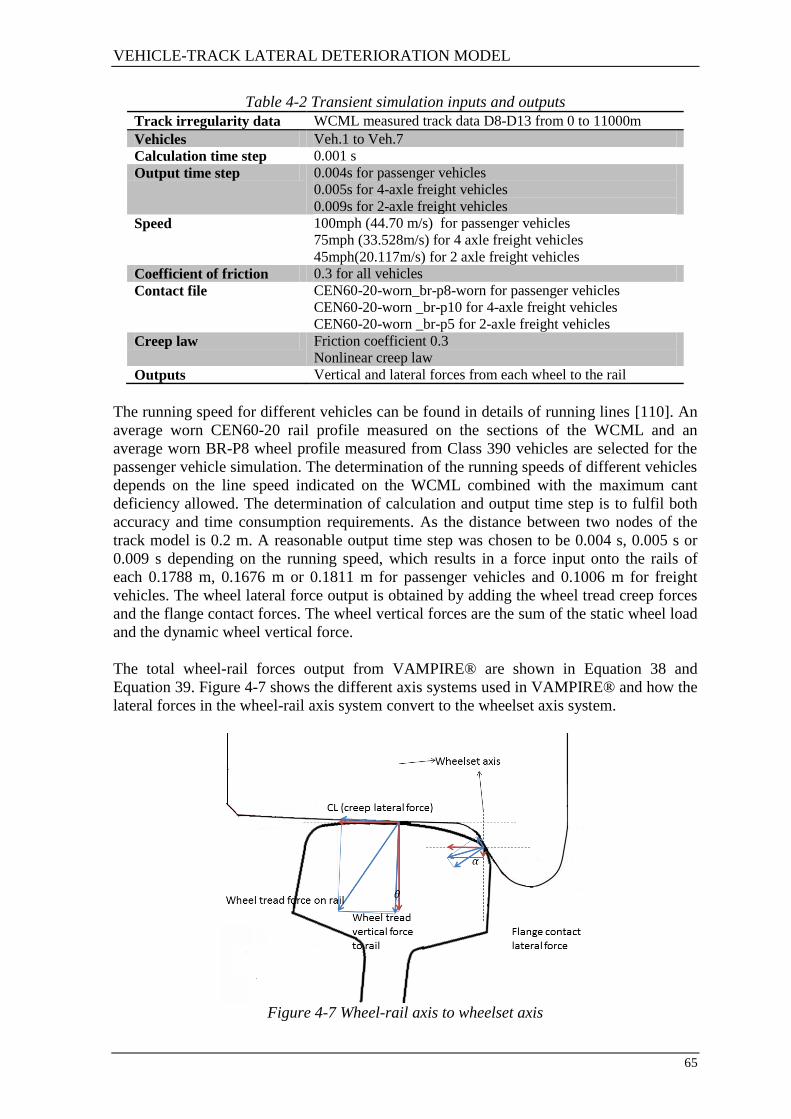
VEHICLE-TRACK LATERAL DETERIORATION MODEL
65
Table 4-2 Transient simulation inputs and outputs
Track irregularity data WCML measured track data D8-D13 from 0 to 11000m
Vehicles Veh.1 to Veh.7
Calculation time step 0.001 s
Output time step 0.004s for passenger vehicles
0.005s for 4-axle freight vehicles
0.009s for 2-axle freight vehicles
Speed 100mph (44.70 m/s) for passenger vehicles
75mph (33.528m/s) for 4 axle freight vehicles
45mph(20.117m/s) for 2 axle freight vehicles
Coefficient of friction 0.3 for all vehicles
Contact file CEN60-20-worn_br-p8-worn for passenger vehicles
CEN60-20-worn _br-p10 for 4-axle freight vehicles
CEN60-20-worn _br-p5 for 2-axle freight vehicles
Creep law Friction coefficient 0.3
Nonlinear creep law
Outputs Vertical and lateral forces from each wheel to the rail
The running speed for different vehicles can be found in details of running lines [110]. An
average worn CEN60-20 rail profile measured on the sections of the WCML and an
average worn BR-P8 wheel profile measured from Class 390 vehicles are selected for the
passenger vehicle simulation. The determination of the running speeds of different vehicles
depends on the line speed indicated on the WCML combined with the maximum cant
deficiency allowed. The determination of calculation and output time step is to fulfil both
accuracy and time consumption requirements. As the distance between two nodes of the
track model is 0.2 m. A reasonable output time step was chosen to be 0.004 s, 0.005 s or
0.009 s depending on the running speed, which results in a force input onto the rails of
each 0.1788 m, 0.1676 m or 0.1811 m for passenger vehicles and 0.1006 m for freight
vehicles. The wheel lateral force output is obtained by adding the wheel tread creep forces
and the flange contact forces. The wheel vertical forces are the sum of the static wheel load
and the dynamic wheel vertical force.
The total wheel-rail forces output from VAMPIRE® are shown in Equation 38 and
Equation 39. Figure 4-7 shows the different axis systems used in VAMPIRE® and how the
lateral forces in the wheel-rail axis system convert to the wheelset axis system.
Figure 4-7 Wheel-rail axis to wheelset axis

VEHICLE-TRACK LATERAL DETERIORATION MODEL
66
Equation 38
Equation 39
Where,
and … total wheel-rail vertical and lateral force
W … static vertical force
… dynamic vertical force
… angle of wheel/rail tread contact from horizontal
… angle of flange contact from horizontal
… lateral creep force on wheel-rail axis system
… flange creep force on wheel-rail axis system
… flange normal force on wheel-rail axis system
4.1.5 Conclusion
The VAMPIRE® simulation tool has been explained in detail in terms of its inputs and
outputs. Firstly, the parameters of the track irregularity input file were described, and track
sections S15-S17 and S10 of D8-D13 from Chapter 3.3 were selected for the analysis.
Secondly, different wheel-rail contact conditions were compared and the measured worn
rail and wheel profiles were selected for the simulation. Then, seven models of vehicles
which run on the particular section of track of the WCML were developed. Finally, the
calculation step and running speeds are determined according to the different vehicle types,
and the resultant vertical and lateral dynamic forces between the wheels and rails are
described.
4.2 Track parameters
Track parameters describe the characteristics of the track, and track in different conditions
and locations may have different representative parameter values. The development of
different track parameters is based on many studies which involve complicated
measurement and lab tests. Accurate track parameters give a better understanding of the
track system and the selection of track parameters plays an essential role in track model
development. In this section, all the important track parameters that are used in the lateral
track deterioration model will be presented and described in detail. For validation purpose
the track parameters are selected to represent as best as possible the WCML track
condition.

VEHICLE-TRACK LATERAL DETERIORATION MODEL
67
4.2.1 Track stiffness and damping
In the track model, the sleeper is considered rigid and the ballast, sub-ballast and geotextile
layers are considered as a whole subsystem in order to reduce the complexity. Track
stiffness and damping are the fundamental track parameters, which describe the elastic
characteristics of the track. These play an important role in vehicle-track dynamic
behaviour. Many studies have pointed out that the track stiffness has a significant influence
on track dynamic performance. Esveld [111] claimed that track stiffness has been found to
be useful for determining the cause of certain subgrade problems. Sussmann et al. [112]
stated that track stiffness can be used to provide an additional indicator of track condition
to inspectors and to guide maintenance planning and execution. It is also asserted by
Fröhling [113] that spatial variation of the track stiffness contributes significantly to track
deterioration, both in terms of differential track settlement and increased dynamic vehicle
loading. Relatively high track stiffness is beneficial in that it provides sufficient track
resistance to loads, however, track stiffness that is too high can cause increased dynamic
forces in the wheel-rail interface as well as on sleepers and ballast, which may lead to wear
and fatigue of track components [114]. The damping of the track has a large impact on the
dynamic reactions, and an increase in damping can effectively reduce rolling noise [115].
Consequently it is important to have a good understanding of the track in order to select the
right stiffness value in the model development process.
The stiffness values between two adjacent components should be determined. As it is a
triple layered track model, the stiffness values considered are the rails, rail pads and
fastenings stiffness, as well as the track bed stiffness. The stiffness of different track layers
can be measured from laboratory tests. Normally, the force-deflection relationship has the
nonlinear characteristic shown in Figure 4-8 [116] and also includes some degree of
hysteresis.
Figure 4-8 Force-deflection diagram of track with quasi-static excitation
However, the track stiffness (k) is most commonly approximated as a linear relationship
shown in Equation 40, where the track stiffness is the ratio of applied load on the track (F)
and the track deflection (z) at a certain force level.
Equation 40
The global stiffness takes the whole track structure into account, and can be measured by
several existing methods. Liu and Wang [117] claimed that a reasonable range of global
stiffness is between 62 kN/mm and 87 kN/mm per rail for ballast track. For the track
system, the series of stiffnesses in diffent layers is shown in Figure 4-9.
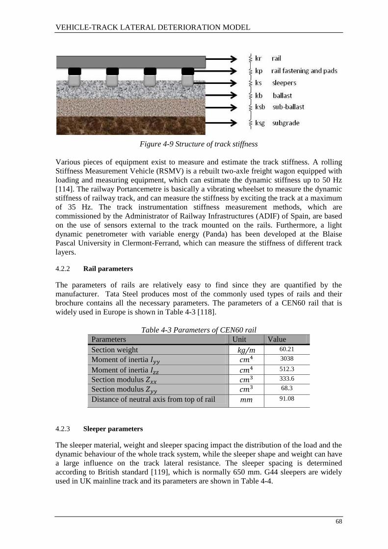
VEHICLE-TRACK LATERAL DETERIORATION MODEL
68
Figure 4-9 Structure of track stiffness
Various pieces of equipment exist to measure and estimate the track stiffness. A rolling
Stiffness Measurement Vehicle (RSMV) is a rebuilt two-axle freight wagon equipped with
loading and measuring equipment, which can estimate the dynamic stiffness up to 50 Hz
[114]. The railway Portancemetre is basically a vibrating wheelset to measure the dynamic
stiffness of railway track, and can measure the stiffness by exciting the track at a maximum
of 35 Hz. The track instrumentation stiffness measurement methods, which are
commissioned by the Administrator of Railway Infrastructures (ADIF) of Spain, are based
on the use of sensors external to the track mounted on the rails. Furthermore, a light
dynamic penetrometer with variable energy (Panda) has been developed at the Blaise
Pascal University in Clermont-Ferrand, which can measure the stiffness of different track
layers.
4.2.2 Rail parameters
The parameters of rails are relatively easy to find since they are quantified by the
manufacturer. Tata Steel produces most of the commonly used types of rails and their
brochure contains all the necessary parameters. The parameters of a CEN60 rail that is
widely used in Europe is shown in Table 4-3 [118].
Table 4-3 Parameters of CEN60 rail
Parameters Unit Value
Section weight kg/m 60.21
Moment of inertia 3038
Moment of inertia 512.3
Section modulus 333.6
Section modulus 68.3
Distance of neutral axis from top of rail mm 91.08
4.2.3 Sleeper parameters
The sleeper material, weight and sleeper spacing impact the distribution of the load and the
dynamic behaviour of the whole track system, while the sleeper shape and weight can have
a large influence on the track lateral resistance. The sleeper spacing is determined
according to British standard [119], which is normally 650 mm. G44 sleepers are widely
used in UK mainline track and its parameters are shown in Table 4-4.
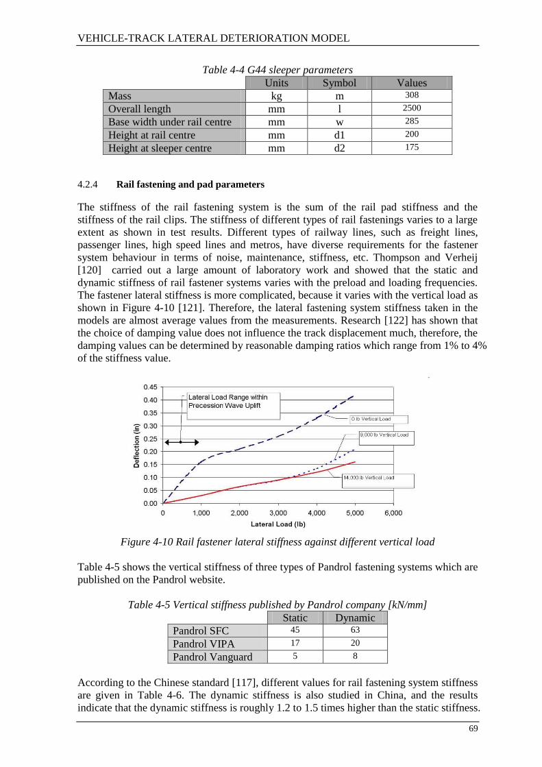
VEHICLE-TRACK LATERAL DETERIORATION MODEL
69
Table 4-4 G44 sleeper parameters
Units Symbol Values
Mass kg m 308
Overall length mm l 2500
Base width under rail centre mm w 285
Height at rail centre mm d1 200
Height at sleeper centre mm d2 175
4.2.4 Rail fastening and pad parameters
The stiffness of the rail fastening system is the sum of the rail pad stiffness and the
stiffness of the rail clips. The stiffness of different types of rail fastenings varies to a large
extent as shown in test results. Different types of railway lines, such as freight lines,
passenger lines, high speed lines and metros, have diverse requirements for the fastener
system behaviour in terms of noise, maintenance, stiffness, etc. Thompson and Verheij
[120] carried out a large amount of laboratory work and showed that the static and
dynamic stiffness of rail fastener systems varies with the preload and loading frequencies.
The fastener lateral stiffness is more complicated, because it varies with the vertical load as
shown in Figure 4-10 [121]. Therefore, the lateral fastening system stiffness taken in the
models are almost average values from the measurements. Research [122] has shown that
the choice of damping value does not influence the track displacement much, therefore, the
damping values can be determined by reasonable damping ratios which range from 1% to 4%
of the stiffness value.
Figure 4-10 Rail fastener lateral stiffness against different vertical load
Table 4-5 shows the vertical stiffness of three types of Pandrol fastening systems which are
published on the Pandrol website.
Table 4-5 Vertical stiffness published by Pandrol company [kN/mm]
Static Dynamic
Pandrol SFC 45 63
Pandrol VIPA 17 20
Pandrol Vanguard 5 8
According to the Chinese standard [117], different values for rail fastening system stiffness
are given in Table 4-6. The dynamic stiffness is also studied in China, and the results
indicate that the dynamic stiffness is roughly 1.2 to 1.5 times higher than the static stiffness.

VEHICLE-TRACK LATERAL DETERIORATION MODEL
70
Table 4-6 Rail fastening system vertical stiffness in Chinese standard [kN/mm]
Freight lines 70 ~ 90
Freight and passenger mix lines 50 ~ 80
Passenger lines 50 ~ 70
Slab track lines 30 ~ 50
These two tables give a general idea of the rail fastening system stiffness range. The
stiffness value used in the track model is usually the stiffness of rail-fastening-sleeper
assembly system. 5 types of commonly used rail fastening systems assembled with CEN
60 rail and half G44 sleeper were tested at the University of Birmingham [123] for the
Crossrail project, and Table 4-7 shows the measured stiffness of these tests under 60 kN
preload. It shows a large difference between the different rail fastening systems.
Table 4-7 Quasi-static CEN60-rail fastening system-half G44 sleeper assembly test under
60kN preload [kN/mm]
Pandrol
E-clip
Pandrol
SFC
Pandrol
VIPA
Pandrol
Vanguard
DELKOR
60 kN preload
Vertical 120.7 108.5 12.3 7.4 12.2
Lateral 41.4 54.4 10.1 62.7 10.8
The dynamic stiffness of two assemblies, which are widely used on British mainline
railways, can be found in Pandrol test reports. The parameters of the 60E1 and 56E1
assemblies are summarised from Pandrol test reports No.41174 and No.45111 and the
average value of the test results are shown in Table 4-8. The results were not always
consistent in the lateral direction. The reason may be the fact that the effective stiffness at
the rail head is different because of the contribution of rail roll.
Table 4-8 Summary of Pandrol report [kN/mm] Properties 60E1 assembly 56E1 assembly
Vertical 270 200
Lateral 400 250
Equivalent lateral head stiffness 398 250
60E1 assembly: G44 sleepers - clips FC1504 – CEN60
56E1 assembly: G44 sleepers – clips FC1504 – BS113A
Bezin [124] selected and summarised both the quasi-static and dynamic parameters of the
rail pads, and are shown in Table 4-9.
Table 4-9 Summarised rail pad parameters Quasi-static Dynamic
Stiffness [kN/mm] Stiffness [kN/mm] Damping [kN.s/m]
Soft rail pad 75 150 20
Typical rail pad 150 300 30
Stiff rail pad 500 1000 50
The rail pad vertical parameters are summarised from receptance tests [125], and are
shown in Table 4-10.

VEHICLE-TRACK LATERAL DETERIORATION MODEL
71
Table 4-10 Rail pad parameters Pad section Stiffness [kN/mm] Damping [kN.s/m]
Railtrack FC584 480 49
DB AG ZW900 196 32
SNCF 9mm rubber 500 30
4.2.5 Track bed parameters
The subgrade modulus is the most variable quantity among all of the track parameters due
to change of soil type, environmental conditions and stress state. Therefore, the track bed
stiffness of the same type of track can be different in different locations. In the lateral
direction, the sleeper tends to behave in a highly nonlinear manner. The sleeper behaves
relatively linearly below a certain force limit, above which it slides. Furthermore, it is
difficult to measure the lateral properties. An indicative value of the ballast lateral stiffness
was measured by Clark et al. and the typical track bed stiffness is summarised in Table
4-11 [126].
Table 4-11 Summary of track bed stiffness per sleeper Vertical Lateral
Quasi-static Dynamic Quasi-static
Stiffness
kN/mm
Stiffness
kN/mm
Damping
kN.s/m
Stiffness
kN/mm
Damping
kN.s/m
Soft track bed 10 20 50 - -
Typical track bed 40 80 100 40 240
Stiff track bed 100 200 150 - -
The sleeper vertical support stiffness on the East Coast Main Line (ECML) is measured in
four different locations and summarised in Table 4-12 [127].
Table 4-12 Quasi-static stiffness measurements at various sites Site name
(all on ECML)
Sleeper support stiffness
kN/mm per sleeper
Dry Doddington 43
Gamston 35
Retford 51
Noblethorpe 28
Sun and Dhanasekar [62] outlined the track parameters from four different track studies
and the sleeper stiffness and damping coefficients are shown in Table 4-13.
Table 4-13 Sleeper support parameter in four different researches Dong
et al.
Newton
and
Clark
Fermér
and
Nielsen
Zhai
Sleeper stiffness (kN/mm) 31.6 79 98 98
Sleeper damping (kN.s/m) 21.8 50 130 130
The track bed parameters are also summarised in a Chinese report [65] shown in Table
4-14. These parameters represent the entire track bed including ballast, sub-ballast and
subgrade, so it is larger than the actual sleeper-ballast interface properties.

VEHICLE-TRACK LATERAL DETERIORATION MODEL
72
Table 4-14 Track bed parameters Vertical Lateral
Stiffness [ ] 100-400 40-60
Damping [ ] 80-150 25-30
There are a few laboratory tests that have looked at these non-linear relationships between
sleeper and ballast listed in Appendix D, and these are summarised in Table 4-15. It is
found that the lateral stiffness is around 4kN/mm in the unloaded condition.
Table 4-15 Lateral Resistance Characteristic Values per Sleeper
Elastic
resistance
Fe (kN)
Elastic
displaceme
nt we (mm)
Break-
away force
Fp (kN)
Break-away
displaceme
nt wp (mm)
Sliding
resistance
Fl (kN)
Sliding
displacement
wl(mm)
Loose Tamped/Relay (Weak) 2.4 0.6 8 3 5.2 40
Just Tamped/Undisturbed (Medium) 2.8 0.8 9.8 3.5 6.2 40
Trafficked (Strong) 4.0 1.0 13.3 4.8 6.7 40
Lateral ballast stiffness is considered to be 4000 kN per square metre; when the lateral
resistance of the ballast is reduced to 800 kN per square metre the lateral displacements
become large [128]. Field test results [129] give a lateral ballast resistance value of 95.2
kN per centimetre per sleeper spacing. The ballast lateral stiffness is considered to be
per square metre in a high frequency wheel-rail interaction model in both the
vertical and lateral directions [130]. The units of these stiffness values are transformed into
consistent values as shown in Table 4-16.
Table 4-16 Summary of ballast lateral stiffness in different studies Original value in different units to
uniformed unit
4
15.87
133
It can be seen that the ballast lateral stiffness values varies by a large amount. The reason
may be that the different studies have different track bed properties. It is difficult to find
any research that studied or tested the ballast lateral stiffness and damping in detail.
Another reason may be that the highly non-linear characteristic of the sleeper-ballast
interface makes it difficult to obtain reliable test results. In this study, the interface between
the sleeper and ballast is more important, therefore the sub-ballast and subgrade layers can
be considered rigid supporting the ballast layer. Single Tie Push Tests (STPT) were carried
out by Sussmann et al. [131] to investigate the lateral resistance of concrete sleepers, and
the average peak lateral resistance range of a concrete tie was between 8.4kN to16.1kN
with strong condition within a displacement of 25mm. Figure 4-11 shows the load-
displacement relationship of a concrete sleeper and the stiffness of the single tie can be
estimated at around 4-8kN/mm.

VEHICLE-TRACK LATERAL DETERIORATION MODEL
73
Figure 4-11 Characteristic of lateral resistance measurement
4.2.6 Friction coefficient
This is the friction coefficient defined by the ratio of sleeper lateral force resistance to
vertical loading force. In most analyses the friction coefficient is taken at a constant value
of around 0.8 for concrete sleepers. However, the friction value varies with the different
vertical load Kish et al. [93] describe the change of friction coefficient with the dynamic
vertical load in an analytical equation as shown below.
Equation 41
Where,
…the vertical load
…the friction coefficient at zero vertical load
…the coefficient at large vertical load
…constant parameter
Table 4-17 shows the value of the constants in the friction coefficient equation for both
wooden and concrete sleepers.
Table 4-17 Values of constants for wood and concrete sleepers [93] (1/kN)
Concrete sleeper 0.9 0.75 0.71
Wooden sleeper 1.15 0.68 0.49

VEHICLE-TRACK LATERAL DETERIORATION MODEL
74
Figure 4-12 shows the resulting tie-ballast friction coefficient as a function of vertical
sleeper force for both wooden and concrete.
Figure 4-12 Friction coefficient varies with vertical force [93]
These ‘friction’ parameters are tested based on the sleeper-ballast interface, which includes
the bending forces from the rails. In the track shift model, only the interface between an
individual sleeper and the ballast is considered.
The lateral resistance tests indicate the friction coefficient to be around 0.5, while the
friction between ballast particles is in the range of 0.9 to 1.4 [132] [133]. Meanwhile,
other studies claim a friction coefficient between a concrete sleeper and ballast of roughly
0.1 [134] [135]. The lateral to vertical loading ratio which can be considered as the friction
coefficient between sleeper base and ballast is found to be around 0.45 from lab tests in the
University of Southampton [77]. The required lateral to vertical loading ratio tends to
slightly reduce after the peak lateral resistance.
Therefore, the friction coefficient between the sleeper and ballast at zero and large vertical
load can be estimated in proportion to the coefficient for sleepers. Table 4-18 shows the
estimated friction coefficient for different sleeper-ballast contact conditions.
Table 4-18 Possible residual and friction coefficient values for simulation
0.01 0.45
0.0083 0.3735
(1/kN) 0.71 0.71
The coefficient is selected as 0.01 for residual deflection simulations, while a bigger
friction coefficient of 0.45 will be used to determine sliding failure. In addition, the values
of and should decrease with the number of load passes due to the ballast shear and
wear under the cyclic sleeper movements. The percentage reduction in these constants is
calculated to be 0.05% per pass or 5% for 100 passes.

VEHICLE-TRACK LATERAL DETERIORATION MODEL
75
Figure 4-13 Friction coefficient reduction over loading passes
However, according to the traffic mix given in Chapter 4.4.2 there will be more than 10000
axle passes within a month and a large number of maintenance activities taking place on an
operational railway line such as the WCML, and this linear reduction will not be valid. In
order to include the friction reduction, and at the same time make it easier in the simulation,
a 5% reduction of friction coefficient per 20000 axle passes is used to estimate the real
situation.
4.2.7 Conclusion
It was found that the track component stiffness and damping are mainly measured and
investigated in the vertical direction. The references for lateral track behaviour and
parameters are limited due to its complicated interface and the highly nonliner dynamic
behaviour. It is straightforward to find the parameters for rails, rail fasteners, pads and
sleepers, because enough information is available from industry suppliers. The stiffness
and damping values of the sleeper-ballast interface is more difficult, due to lack of
dynamic behaviour information of the track bed. Test results and meausrements are
required to study and compare the parameters of sleeper-ballast interface in detail. The
additional sleeper-ballast interface pararameters, including the lateral resistance
characteristics and friction coefficient, are also studied in order to have a better
understanding of the non-linear characteristic of this interface.
4.3 Track lateral shift model
A Finite Element (FE) model was selected to investigate the non-linear lateral behaviour of
the track. Although it is widely used in engineering, the drawback is that it can be time
consuming to model a complete track system due to the large number of elements and
degrees of freedom required [76]. Track lateral settlement is caused by multiple passages
of vehicles that would take an extremely long time to calculate using FE modelling.
In the single sleeper lateral shift analysis, the bending behaviour of the sleeper is simplified
to have a linear relationship with the rail deflection. This can lead to an inaccurate analysis
result, thus it is necessary to model the rail bending for a certain length of the track. In the
track lateral shift analysis, the nonlinear factors are inevitable consequently an FE model is
best suited to describe the behaviour of the rail, sleepers and track bed.

VEHICLE-TRACK LATERAL DETERIORATION MODEL
76
Unlike the lateral shift model for a single sleeper, the rail is not supported continuously but
by each sleeper. Therefore, the nodes are defined above every sleeper on the rail as shown
in Figure 4-14. The rails are divided by the length of the sleeper distance to create the
discrete rail elements. When there are N nodes on the rail, there will be N sleepers and N-1
rail elements. For the lateral model only the track behaviour in the lateral direction is
considered, so every rail node has 2 DOF which means that the total rail DOF is 2N.
Figure 4-14 FE track model
The equations of motion of the track lateral shift model are defined in Equation 42 based
on the principle of total potential energy of a dynamic system [136].
{ } { } { } { } Equation 42
The formulation of the model is made in two steps. After the FE rail model is built, the
MBS model of the discrete sleeper and continuous track bed support will be added into the
model.
4.3.1 FE rail model
Assuming on the ith
rail element, moment , and lateral forces , are applied
respectively on node i and i+1, as shown in Figure 4-15. The rail element displacement
vector is:
{ } {
{ }
{ } } [
] Equation 43
Where,
, … the displacement of each node
, … the roll angle of each node

VEHICLE-TRACK LATERAL DETERIORATION MODEL
77
Figure 4-15 Rail element load and displacement condition
There are several different methods used to obtain the stiffness matrix of the rail element:
Hermite interpolation[137], direct stiffness method and principle of virtual work [138].
The Hermite interpolation method is selected in this study due to its convenience in finding
out the complete mass, damping and stiffness matrix. Therefore, the displacement of the
rail element on any point is:
{ } Equation 44
In which,
Equation 45
Where,
{
(
)
(
)
[ (
) (
)
]
(
)
(
)
[(
)
]
Equation 46
The vibration kinetic energy and bending strain energy of the rail element are respectively:
∫
{ }
*∫
+ { } Equation 47
∫ (
)
{ }
[∫ (
)
(
)
] { }
Equation 48
Substituting Equation 46 into Equation 47 and integrating, the mass matrix of the rail
element is established as:
[
] Equation 49

VEHICLE-TRACK LATERAL DETERIORATION MODEL
78
Substituting Equation 46 into Equation 48 and integrating, the stiffness matrix of the rail
element is:
[
] Equation 50
Assuming there is a concentrated load P(t) on x=l, then the virtual work done by the force
is:
{ } Equation 51
So, the force on the element is expressed as
{ }
Equation 52
4.3.2 Track lateral model development
According to the track lateral model shown in Figure 4-14, the unknown lateral
displacement vector and the input force matrix of the two rails nodes and the sleepers are
written as:
{ }
[
]
{ }
[
]
Equation 53
The same principle and method are used to build the complete track lateral shift model
with N sleepers. The vibration kinetic energy, bending strain energy and the virtual work
of the whole track system can be written as:

VEHICLE-TRACK LATERAL DETERIORATION MODEL
79
∑{ }
{ }
∑{ }
{ }
∑
Equation 54
∑{ }
{ }
∑{ }
{ }
∑
∑
∑
Equation 55
∑
∑
{ }
Equation 56
The mass and stiffness matrix of the whole track lateral system can be found from the first
variation of Equation 54 and Equation 55, and the damping stiffness matrix can be found
from Equation 56 (Appendix C.1). Subsequently, a numerical computer simulation model
based on Equation 42 can be built using MATLAB. The Wilson- numerical integration is
chosen to solve Equation 42. When , the Wilson- method will be
unconditionally stable. In the simulation, is taken as 1.4 to ensure the accuracy of the
numerical calculation. Taking each sleeper spacing on the rail as an element, there are 31
sleepers, which means 31 nodes on each of the rails and 155 DOF in total. The track
irregularity profile from the ECML, therefore the 60E1 track fastening is used. The track
properties are described in Table 4-19.
Table 4-19 Selected track parameters for linear simulation
Symbol Units Value
Young modulus E
Section mass of CEN60 rail kg 60
G44 concrete sleeper mass kg 308
Sleeper spacing s m 0.6
Section moment of area about vertical axis
Section moment of area about horizontal axis
Rail pad lateral stiffness
Rail pad lateral damping
Rail pad vertical stiffness
Rail pad vertical damping
Sleeper-ballast lateral stiffness N/m
Sleeper-ballast lateral damping
Sleeper-ballast vertical stiffness
Sleeper-ballast vertical damping
Young modulus E

VEHICLE-TRACK LATERAL DETERIORATION MODEL
80
When there are similar 30 kN loads on both rails, moving from the first node to the last at a
speed of 33.35 m/s. The simulation gives a result of the centre rail node movement, shown
in Figure 4-16.
Figure 4-16 Centre rail node displacement and input vertical forces
The simulation results were found to be reasonable, and the shape of the rail deflection
graph is quite similar to the BOEF static force output. However, the dynamic response can
be different, and VAMPIRE is used to generate the dynamic lateral force input on the track.
Figure 4-17 shows the centre rail node dynamic response when a four-axle vehicle runs
along the track at 33.5m/s. The input force matrix is captured from the VAMPIRE
simulation of a Class 365 EMU using measured ECML track data. The recorded site data
has some small lateral irregularities, which cause the vibration of the vehicle-track system.
Figure 4-17 Dynamic response of the centre of rail and lateral force input from VAMPIRE

VEHICLE-TRACK LATERAL DETERIORATION MODEL
81
It is found that the dynamic lateral force is small, between 4 and 10 kN, thus it is difficult
to reach the lateral to vertical load ratio failure point which is the triggering limit of the
track lateral sliding according to the laboratory test results by the University of
Southampton [77]. Normal track lateral irregularities do not excite the vehicle sufficiently
to produce enough lateral force to move the sleeper laterally. Therefore, large irregularities
of the track are required for ballast rearrangement and track lateral sliding.
The peak lateral displacements are important in determining if the failure point is reached.
The previous simulation was conducted with only 2 nodes on each element, which means
that only the sleeper and rail contact point is considered, and the rail bending is simplified.
Therefore, the elements with 2 to 7 nodes are simulated, and the result is shown in Figure
4-18. It is clear that the more nodes that are considered, the more accurate the results.
However, more nodes lead to longer calculation times. When the number of nodes on the
element is more than 4, the peak displacements are quite similar.
Figure 4-18 Simulation results with different number of nodes
However, more nodes lead to exponential increase in calculation time, as shown in Table
4-20. Considering the calculation speed, 4 nodes between adjacent sleepers are selected to
give a good balance between accuracy and calculation time.
Table 4-20 Simulation time for a 30 m section of track
Num. of nodes between
adjacent sleepers
2 3 4 5 6 7
Simulation time [min] 0.83 2.5 7.8 19.3 39.7 70.5

VEHICLE-TRACK LATERAL DETERIORATION MODEL
82
4.3.3 Define the non-linear load-deflection relationship
The lateral track model is a linear FE model which can only describe the track system
vibration behaviour. However in reality, the track lateral position may not be restored after
vehicle passages due to the residual and frictional characteristics of the sleeper-ballast
interface, so the failure of this interface, which causes sliding is not detected. Kish et al.
[93] claimed that both the theory and the test data indicate that the residual deflection has
an exponential growth at first, and then tends to increase in an almost linear manner after
some initial passes, furthermore, the growth of residual deflection is also found to be
related to lateral to vertical loading ratio L/V, as shown in Figure 4-19.
Figure 4-19 Residual deflection of sleepers versus number of passes
However, in reality the L/V ratio is not a constant value. It changes with different dynamic
vertical and lateral loads, so in the vehicle-track dynamic simulation process the L/V ratio
needs to be calculated at each time step in order to determine the residual or sliding
deflection.
As over 30 years of research and tests have confirmed, lateral resistance is a load versus
deflection nonlinear spring response as illustrated in Figure 4-20, which also includes a
simplified analytic representation [139]. It can be found that the lateral displacement under
peak resistance varies with different track conditions, and the non-linear characteristic is
more force sensitive compared to the displacements. The softened lateral stiffness is also
not a constant value, according to the figure it is a stiffness value close to the elastic lateral
stiffness.
Figure 4-20 Lateral resistance load deflection characteristics

VEHICLE-TRACK LATERAL DETERIORATION MODEL
83
The sleeper stick-slip motion can be classified as an elastic displacement, residual
deflection known as pre-sliding displacement and sliding which is a lateral resistance
failure. Before sliding occurs, there is a linear and non-linear spring-like behaviour which
is also known as hysteresis and the force as function of displacement is shown in Figure
4-21 a). The hysteresis was observed as the velocity varies, and the size of the loop
increases with normal load, viscosity and frequency of the velocity variation. When the
displacement is small and is almost recovered after loading, the behaviour can be seen as
elastic.
a) Pre-sliding displacement [140] b) Break-away and sliding [141]
Figure 4-21 Force-displacement relationship in pre-sliding and sliding
A non-linear relationship exists between the lateral resistance and vertical loading, which
influences the residual deflection, ballast softening and track lateral sliding. The non-linear
lateral resistance characteristic is shown in Figure 4-22 (a), which was determined from
experimental programmes by BR Research [125], DB [142], and TU Delft [143]. The
simplified non-linear characteristic illustrated in Figure 4-22 (b) is employed in the actual
track model in order to make the calculation process easier.
a) Track lateral resistance behaviour in reality (b) Modified force-displacement function
Figure 4-22 Track lateral resistance characteristic
The softening part of the non-linear characteristic is simplified to sliding behaviour in the
model as shown in the figure. In both figures, the dashed black line represents the lateral
resistance without vertical loading on the track, while the dynamic case with vehicle
loading on the track is shown as the red line. The influence factors are described below:

VEHICLE-TRACK LATERAL DETERIORATION MODEL
84
and represent the elastic breaking force and displacement, these elastic limit
values are only related to the sleeper-ballast interface without the influences from
the rails. Thus the value of and are smaller and proved around 5% of the
measured sleeper elastic limit forces and displacements during the model
development and validation.
and are respectively the break-away resistance and displacement, which are
the force and displacement required to overcome the static friction and initiate
motion [144]. They can be seen as the starting point when the sleeper slides
laterally on the ballast bed, which is a serious failure mode. Whenever the forces
exceed this limit, the model stops running and provides a warning.
is the residual deflection stiffness softening factor, the softening factor has a 0.15%
linear reduction for 20000 axle passages. It is found that 0.998 to 0.999 are
reasonable softening factors in the model development process in the test
simulations.
is the vertical force distributed from the rails onto the sleeper.
Even small forces can cause residual deflections and it is not therefore sensible to
use the actual coefficient between the sleeper and ballast in the residual deflection
calculation. For example, the lateral forces are usually less than 5 kN on straight
track, and using the actual friction coefficient which gives a dynamic elastic limit
force of more than 10kN which will not capture any small accumulated residual
deflection after a number of wheel passes. Therefore, a much smaller coefficient is
defined and used in the model for residual deflection calculation. is the residual
coefficient between the sleeper and ballast to determine the residual deflection, and
is the actual friction coefficient between the sleeper and ballast, here is
around 2-3% of . A 5% linear reduction of both residual and friction coefficient
per 20000 axle passes is used in this simulation.
It is important to note that when a vehicle runs on the track, the lateral resistance will be
weaker on the dynamic uplift sections as shown in Figure 4-23.
Figure 4-23 Dynamic lateral resistance influenced by vertical load
The lateral and vertical loads distributed onto each sleeper are used to determine the
sleeper residual or sliding deflections. These distributed forces are the interaction forces
between the rails and sleeper, which can be described in Equation 57.

VEHICLE-TRACK LATERAL DETERIORATION MODEL
85
Equation 57
Where,
, and … rails and sleeper displacements
… stiffness between rails and sleeper
, and … rails and sleeper velocities
… damping between rails and sleeper
After the vertical and lateral distributed loads are captured from the elastic track model, the
sleeper residual and sliding deflection modes can be determined. The method for including
pre-sliding and sliding characteristics into the model is discussed below.
4.3.3.1 Pre-sliding dynamics
All the sleeper displacements will be fully recovered when the lateral force and
displacements are smaller than and as shown in Equation 58.
Equation 58
When the sleeper-ballast interface behaves elastically, the lateral stiffness between the
sleeper and ballast in Figure 4-24 can be calculated from Equation 59.
Equation 59
Figure 4-24 Definition of track lateral pre-sliding behaviour
When the lateral force is larger than the elastic limit force and smaller than the break-away
force (Equation 60), there will be a permanent residual deflection which is represented by
in Figure 4-24. It is important to note that the forces here are the forces that only related
to the stiffness term in the dynamic system. There are other parts of the total force related
to damping and acceleration.

VEHICLE-TRACK LATERAL DETERIORATION MODEL
86
Equation 60
There will be an elastic recovery of the displacement represented by , and the stiffness
between sleeper and ballast will be smaller, and can be calculated from Equation 59.
Equation 61
Where,
…softening factor
The idealized lateral unloading is parallel to the elastic slope, which indicates an elastic
recovery the same as the elastic deflection under the same force. The permanent lateral
residual deflection can be calculated using Equation 62.
Equation 62
It can be found that the slope of the residual deflection has a large influence on the overall
residual deflection thereby having a big effect on track lateral residual deflection.
4.3.3.2 Sliding dynamics
When the lateral force is bigger than the dynamic break-away force, shown in Equation 63,
the sleeper will slide on the ballast layer.
Equation 63
The sliding behaviour can be modelled according to an Iwan friction element [145] as
shown in Figure 4-25.
a) Iwan element b) Stick c) Slip
Figure 4-25 Iwan friction element
The spring-like behaviour does not exist in this failure motion, therefore the stiffness
is considered as 0 without considering the track lateral softening. A large lateral to vertical
loading ratio is required for sliding failure, which means a large defect of the track
alignment. This defect may be caused by accumulated residual deflection from the
dynamic interaction between the vehicle and track. Although the sliding failure is included
in the model, this study mainly focus on the residual deflection component.
4.3.4 Track parameters determination
As described in section 4.3.2, there are 4 nodes on the rail between adjacent sleepers,
which means that there are 3 rail elements between two sleepers. Therefore, the 60 m track
section was modelled with 702 nodes, and at 4 DOF for each rail node and 2 DOF for each
sleeper, there are 2605 DOF in total. All of the track parameters are shown in Table 4-21.
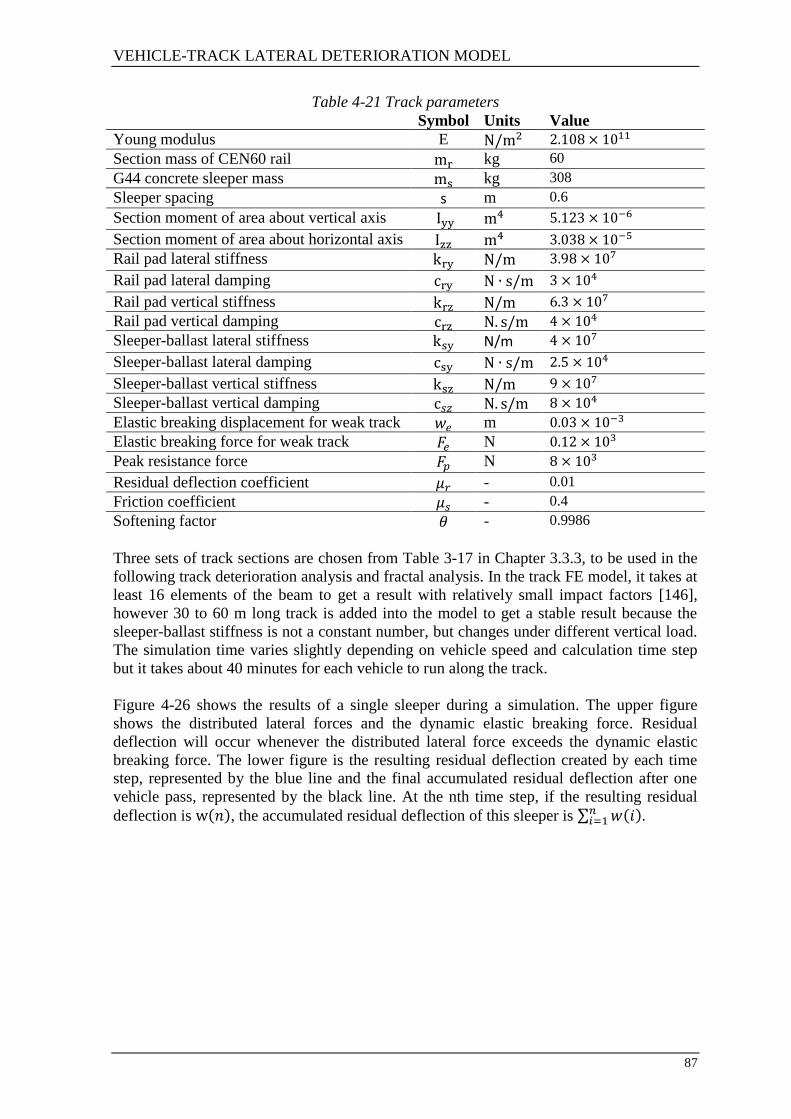
VEHICLE-TRACK LATERAL DETERIORATION MODEL
87
Table 4-21 Track parameters
Symbol Units Value
Young modulus E
Section mass of CEN60 rail kg 60
G44 concrete sleeper mass kg 308
Sleeper spacing s m 0.6
Section moment of area about vertical axis
Section moment of area about horizontal axis
Rail pad lateral stiffness
Rail pad lateral damping
Rail pad vertical stiffness
Rail pad vertical damping
Sleeper-ballast lateral stiffness N/m
Sleeper-ballast lateral damping
Sleeper-ballast vertical stiffness
Sleeper-ballast vertical damping
Elastic breaking displacement for weak track m
Elastic breaking force for weak track N
Peak resistance force N
Residual deflection coefficient - 0.01
Friction coefficient - 0.4
Softening factor - 0.9986
Three sets of track sections are chosen from Table 3-17 in Chapter 3.3.3, to be used in the
following track deterioration analysis and fractal analysis. In the track FE model, it takes at
least 16 elements of the beam to get a result with relatively small impact factors [146],
however 30 to 60 m long track is added into the model to get a stable result because the
sleeper-ballast stiffness is not a constant number, but changes under different vertical load.
The simulation time varies slightly depending on vehicle speed and calculation time step
but it takes about 40 minutes for each vehicle to run along the track.
Figure 4-26 shows the results of a single sleeper during a simulation. The upper figure
shows the distributed lateral forces and the dynamic elastic breaking force. Residual
deflection will occur whenever the distributed lateral force exceeds the dynamic elastic
breaking force. The lower figure is the resulting residual deflection created by each time
step, represented by the blue line and the final accumulated residual deflection after one
vehicle pass, represented by the black line. At the nth time step, if the resulting residual
deflection is , the accumulated residual deflection of this sleeper is ∑ .

VEHICLE-TRACK LATERAL DETERIORATION MODEL
88
Figure 4-26 Single sleeper simulation result
4.3.5 Conclusion
The number of nodes between adjacent sleepers has a big impact on the rail dynamics.
Therefore, the node number is selected as 4 in the following simulation so that the
computation time is low. The rail-sleeper interface is expressed using linear stiffness and
damping elements, whereas the sleeper-ballast interface contains a non-linear characteristic.
This non-linear characteristic includes elastic lateral behaviour, pre-sliding behaviour and
sliding failure.
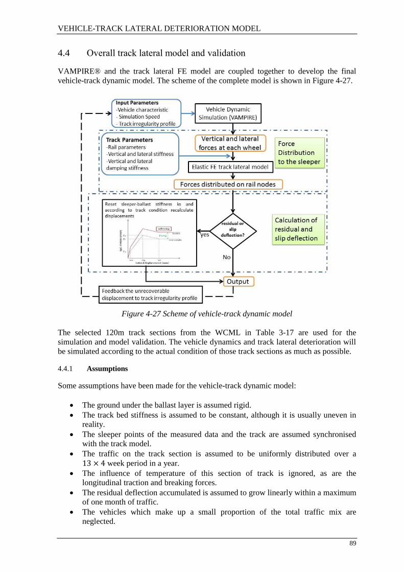
VEHICLE-TRACK LATERAL DETERIORATION MODEL
89
4.4 Overall track lateral model and validation
VAMPIRE® and the track lateral FE model are coupled together to develop the final
vehicle-track dynamic model. The scheme of the complete model is shown in Figure 4-27.
Figure 4-27 Scheme of vehicle-track dynamic model
The selected 120m track sections from the WCML in Table 3-17 are used for the
simulation and model validation. The vehicle dynamics and track lateral deterioration will
be simulated according to the actual condition of those track sections as much as possible.
4.4.1 Assumptions
Some assumptions have been made for the vehicle-track dynamic model:
The ground under the ballast layer is assumed rigid.
The track bed stiffness is assumed to be constant, although it is usually uneven in
reality.
The sleeper points of the measured data and the track are assumed synchronised
with the track model.
The traffic on the track section is assumed to be uniformly distributed over a
week period in a year.
The influence of temperature of this section of track is ignored, as are the
longitudinal traction and breaking forces.
The residual deflection accumulated is assumed to grow linearly within a maximum
of one month of traffic.
The vehicles which make up a small proportion of the total traffic mix are
neglected.

VEHICLE-TRACK LATERAL DETERIORATION MODEL
90
The track irregularity file is not absolute, but filtered at 70m for both vertical and
lateral irregularity data.
The residual and slipping deflections from each sleeper are interpolated using
splines and distributed on to the rails with all the high frequency changes filtered
out.
Only tamping and stone blowing maintenance activities are considered and are
evenly distributed over a week period in a year.
4.4.2 Traffic mix
The detailed traffic data of this section of the WCML is shown in Appendix D.1 during a
week period in a year, and it is summarised to Table 4-22.
Table 4-22 Summarise of traffic information
Total wheelsets passages 135990
Type of vehicle Traffic percentage [%] Total wheelsets pass
390 Motor 53.88 73272
390 Trailer 26.94 36636
221 Motor 6.02 8180
FEAB 3.14 4264
FSAO 3.11 4232
MKIII 1.09 1480
FTAI 0.77 1048
IPAV 0.75 1016
KFAF 0.64 876
MKII 0.38 520
Class 66 Locomotive 0.37 504
Assuming that the traffic is evenly distributed against time, the wheelset passages can be
easily found for each type of vehicle between every measured track dataset, as shown in
Table 4-23.
Table 4-23 Traffic scenario between measured track datasets
Du
ration
as a
percen
tage in
a
perio
d
39
0 M
oto
r
39
0 T
railer
22
1 M
oto
r
FE
AB
FS
AO
MK
III
FT
AI
IPA
V
KF
AF
MK
II
Class 6
6
Lo
com
otiv
e
14/04/2010 Wheelsets passages between two measured data sets
09/06/2010 0.1538 11273 5636 1258 656 651 228 161 156 135 80 78
14/07/2010 0.0962 7045 3523 787 410 407 142 101 98 84 50 48
11/08/2010 0.0769 5636 2818 629 328 326 114 81 78 67 40 39
13/10/2010 0.1731 12682 6341 1416 738 732 256 181 176 152 90 87
08/12/2010 0.1538 11273 5636 1258 656 651 228 161 156 135 80 78
19/01/2011 0.1154 8454 4227 944 492 488 171 121 117 101 60 58
16/03/2011 0.1538 11273 5636 1258 656 651 228 161 156 135 80 78
18/05/2011 0.1731 12682 6341 1416 738 732 256 181 176 152 90 87
15/06/2011 0.0769 5636 2818 629 328 326 114 81 78 67 40 39
20/07/2011 0.0962 7045 3523 787 410 407 142 101 98 84 50 48
17/08/2011 0.0769 5636 2818 629 328 326 114 81 78 67 40 39
14/09/2011 0.0769 5636 2818 629 328 326 114 81 78 67 40 39

VEHICLE-TRACK LATERAL DETERIORATION MODEL
91
16/11/2011 0.1731 12682 6341 1416 738 732 256 181 176 152 90 87
18/01/2012 0.1731 12682 6341 1416 738 732 256 181 176 152 90 87
15/02/2012 0.0769 5636 2818 629 328 326 114 81 78 67 40 39
18/04/2012 0.1731 12682 6341 1416 738 732 256 181 176 152 90 87
18/07/2012 0.25 18318 9159 2045 1066 1058 370 262 254 219 130 126
It is important to be aware of the loading condition of the freight wagons in the simulation,
which can lead to quite different results. The blue line in Figure 4-28 shows the
distribution of the freight vehicle loading condition. As the freight traffic only makes up a
small percentage of the overall traffic, the percentage of tare and laden vehicles can be
approximated from this figure. Any axle load less than 13kN is considered as a tare wagon,
while axle loads of more than 13kN are considered as laden wagons. Therefore, almost 41%
of the traffic is tare and 59% of the traffic is laden.
Figure 4-28 Distribution of freight vehicle loading condition [147]
According to Section 4.1.3, there will be 7 VAMPIRE® vehicle models to represent the
majority of vehicles. The vehicle models and the corresponding wheelset passages are
shown in Table 4-24.
Table 4-24 Traffic scenario for later simulation
Class390 Class221
MKII &
KIII
FEAB,
FSAO,
FTAI,
KFAF
laden
FEAB,
FSAO,
FTAI,
KFAF
tare
IPAV
laden
IPAV
tare
Veh.1 Veh.2 Veh.3 Veh.4 Veh.5 Veh.6 Veh.7
D1 14/04/2010 Wheelsets passages between two measured data sets
D2 09/06/2010 16909 1258 308 946 657 46 32
D3 14/07/2010 10568 787 192 591 411 29 20
D4 11/08/2010 8454 629 154 473 329 23 16
D5 13/10/2010 19023 1416 346 1064 739 52 36
D6 08/12/2010 16909 1258 308 946 657 46 32
D7 19/01/2011 12682 944 231 709 493 35 24

VEHICLE-TRACK LATERAL DETERIORATION MODEL
92
D8 16/03/2011 16909 1258 308 946 657 46 32
D9 18/05/2011 19023 1416 346 1064 739 52 36
D10 15/06/2011 8454 629 154 473 329 23 16
D11 20/07/2011 10568 787 192 591 411 29 20
D12 17/08/2011 8454 629 154 473 329 23 16
D13 14/09/2011 8454 629 154 473 329 23 16
D14 16/11/2011 19023 1416 346 1064 739 52 36
D15 18/01/2012 19023 1416 346 1064 739 52 36
D16 15/02/2012 8454 629 154 473 329 23 16
D17 18/04/2012 19023 1416 346 1064 739 52 36
D18 18/07/2012 27477 2045 500 1537 1068 75 52
4.5 Model validation
Four 60 m sections of track are used in the validations which are S10, S15, S16 and S17
from Table 3-10. The measured and predicted track lateral irregularities were compared, as
well as the measured and calculated track lateral deterioration.
S15 results
Figure 4-29 a) and b) are respectively the measured and predicted track lateral
irregularities. The result indicates a good match between actual measurements and
prediction of track deterioration.
Figure 4-30 a) shows the comparison between measured and predicted lateral deterioration,
which is the difference between two measured track lateral irregularities. Figure 4-30 b)
illustrates the SD value of this section of track, as well as the RMS and correlation
coefficient values of the measured and predicted lateral deterioration. The RMS value
indicates the magnitude of the difference between measured and predicted lateral
deterioration, therefore, the larger the RMS value is the less accurate the prediction. The
correlation coefficient measures the linear correlation between the measured and predicted
deterioration.
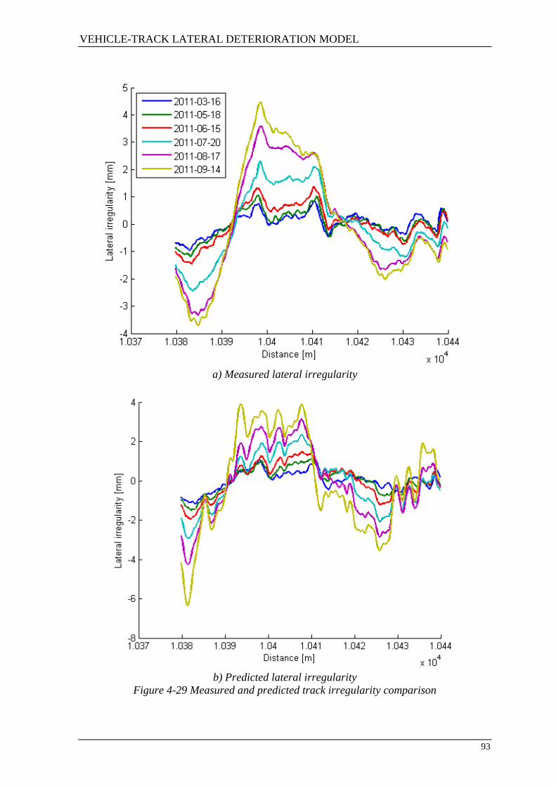
VEHICLE-TRACK LATERAL DETERIORATION MODEL
93
a) Measured lateral irregularity
b) Predicted lateral irregularity
Figure 4-29 Measured and predicted track irregularity comparison

VEHICLE-TRACK LATERAL DETERIORATION MODEL
94
a) Measured and predicted lateral deterioration

VEHICLE-TRACK LATERAL DETERIORATION MODEL
95
b) Precision measures
Figure 4-30 Deterioration comparison and precision measurement

VEHICLE-TRACK LATERAL DETERIORATION MODEL
96
S16 results
a) Measured lateral irregularity
b) Predicted lateral irregularity
Figure 4-31 Measured and predicted track irregularity comparison

VEHICLE-TRACK LATERAL DETERIORATION MODEL
97
a) Measured and predicted lateral deterioration

VEHICLE-TRACK LATERAL DETERIORATION MODEL
98
b) Precision measures
Figure 4-32 Deterioration comparison and precision measurement

VEHICLE-TRACK LATERAL DETERIORATION MODEL
99
S17 results
a) Measured lateral irregularity
b) Predicted lateral irregularity
Figure 4-33 Measured and predicted track irregularity comparison

VEHICLE-TRACK LATERAL DETERIORATION MODEL
100
a) Measured and predicted lateral deterioration

VEHICLE-TRACK LATERAL DETERIORATION MODEL
101
b) Precision measures
Figure 4-34 Deterioration comparison and precision measurement
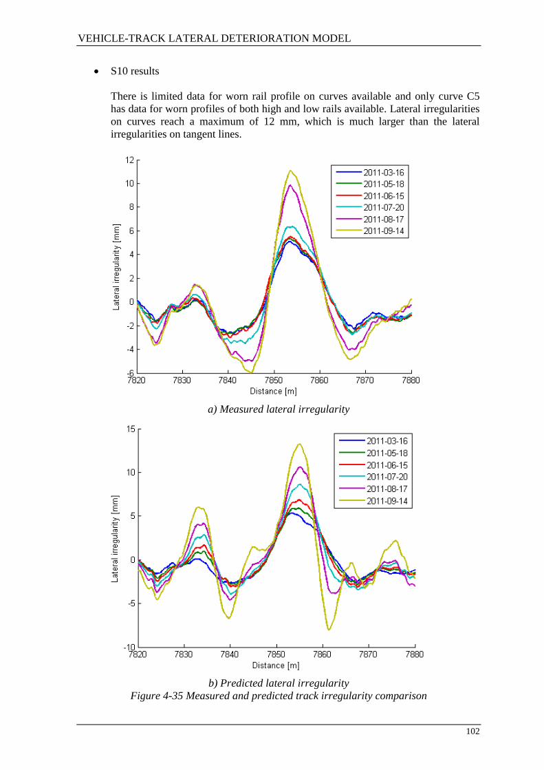
VEHICLE-TRACK LATERAL DETERIORATION MODEL
102
S10 results
There is limited data for worn rail profile on curves available and only curve C5
has data for worn profiles of both high and low rails available. Lateral irregularities
on curves reach a maximum of 12 mm, which is much larger than the lateral
irregularities on tangent lines.
a) Measured lateral irregularity
b) Predicted lateral irregularity
Figure 4-35 Measured and predicted track irregularity comparison

VEHICLE-TRACK LATERAL DETERIORATION MODEL
103
a) Measured and predicted lateral deterioration

VEHICLE-TRACK LATERAL DETERIORATION MODEL
104
b) Precision measures
Figure 4-36 Deterioration comparison and precision measurement

VEHICLE-TRACK LATERAL DETERIORATION MODEL
105
It can be found from these four sets of results that the RMS and correlation values of the
prediction are reasonably accurate for the first 4 to 5 months, and become less accurate
with increasing time. From the actual measured and predicted track lateral irregularities
comparison it can be found that there is an additional small wavelength irregularity in the
prediction results that does not appear in the measured data. The PSD of both the measured
and predicted lateral deterioration are produced for these four sections of track.
Po
wer
Den
sity
[m
m2
/cy
cle/
m]
S1
5
S1
6
S1
7
S1
0
Spatial Frequency [cycle/m]
a) Measured lateral deterioration b) Predicted lateral deterioration
Figure 4-37 Comparison between measured and predicted lateral deterioration PSD

VEHICLE-TRACK LATERAL DETERIORATION MODEL
106
In addition to this major frequency, the predicted deterioration developed a higher
frequency change in the track deterioration between 0.09259 and 0.1389 cycle/m (6.17 to
10.800 m). For the curved element (S10), the additional short wavelength irregularities are
not obvious due to the large magnitude of the long wavelength irregularities. As the
vehicle dynamic forces are the input into the track lateral model, this may be caused by
different vehicle dynamic modes that are excited by different factors. If the 3 to 10.8 m
wavelengths are filtered out from the results, the resulting lateral deterioration is shown
below.
S15 m filtered results
a) Measured lateral irregularity
b) Filtered predicted lateral irregularity
Figure 4-38 Measured and filtered predicted track irregularity comparison

VEHICLE-TRACK LATERAL DETERIORATION MODEL
107
a) Measured and filtered predicted lateral deterioration

VEHICLE-TRACK LATERAL DETERIORATION MODEL
108
b) Precision measures
Figure 4-39 Deterioration comparison and filtered precision measurement

VEHICLE-TRACK LATERAL DETERIORATION MODEL
109
S16 m filtered results
a) Measured lateral irregularity
b) Filtered predicted lateral irregularity
Figure 4-40 Measured and filtered predicted track irregularity comparison

VEHICLE-TRACK LATERAL DETERIORATION MODEL
110
a) Measured and filtered predicted lateral deterioration
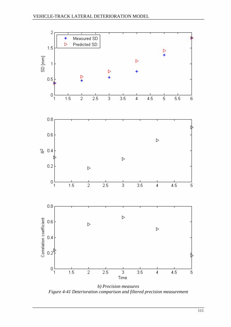
VEHICLE-TRACK LATERAL DETERIORATION MODEL
111
b) Precision measures
Figure 4-41 Deterioration comparison and filtered precision measurement

VEHICLE-TRACK LATERAL DETERIORATION MODEL
112
S17 filtered results
a) Measured lateral irregularity
b) Filtered predicted lateral irregularity
Figure 4-42 Measured and filtered predicted track irregularity comparison

VEHICLE-TRACK LATERAL DETERIORATION MODEL
113
a) Measured and filtered predicted lateral deterioration

VEHICLE-TRACK LATERAL DETERIORATION MODEL
114
b) Precision measures
Figure 4-43 Deterioration comparison and filtered precision measurement

VEHICLE-TRACK LATERAL DETERIORATION MODEL
115
S10 filtered results
a) Measured lateral irregularity
b) Filtered predicted lateral irregularity
Figure 4-44 Measured and filtered predicted track irregularity comparison

VEHICLE-TRACK LATERAL DETERIORATION MODEL
116
a) Measured and filtered predicted lateral deterioration

VEHICLE-TRACK LATERAL DETERIORATION MODEL
117
b) Precision measures
Figure 4-45 Deterioration comparison and filtered precision measurement

VEHICLE-TRACK LATERAL DETERIORATION MODEL
118
The SD values are much better matched, meanwhile, the RMS and correlation coefficient
values indicate much more accurate prediction results with the filtered data. Therefore, it
will be quite important to establish why this certain range of short wavelength deterioration
does not exist in the actual track.
In conclusion, a novel vehicle-track lateral dynamic interaction model has been created to
simulate the link between dynamic behaviour of railway vehicles and track lateral
alignment deterioration, and this model has been validated against recorded track data. It
has been found that the model gives a reasonably accurate prediction of the development of
track irregularities, however it tends to additionally predict a short wavelength
deterioration that is not seen in the actual track deterioration.
4.6 Chapter conclusion
The vehicle-track lateral deterioration model consists of two major sub-models, which are
the vehicle-track dynamic model using VAMPIRE® and the track lateral deterioration
model built in MATLAB. The input factors of both models are studied in detail, so that the
models are set up to match track sections on the WCML as much as possible for model
validation. The model gives a reasonably accurate prediction of the development of track
irregularities, although it tends to additionally predict a short wavelength deterioration that
is not seen in the actual track deterioration.

SENSITIVITY ANALYSIS
119
5 SENSITIVITY ANALYSIS
Different sub-systems of the vehicle-track dynamic system are studied separately and the
influences of them on the track lateral deterioration are discussed. As a result, the
triggering limits in regard to the influences by vehicles, wheel-rail contact conditions and
the track system itself can be identified. For quantities varying both positively and
negatively like track deterioration, RMS is a good measure of the amplitude. Therefore, the
RMS values are used to measure and represent the overall amplitude and amplitude change
of the irregularities.
5.1 Effect of vehicles
The vehicle dynamic impact on track lateral deterioration is discussed in this section. All
parameters used in Chapter 5.1 are those used in the validation for measured data S15 in
dataset D8 referred to in Chapter 4. The influences of different types of vehicles, running
speed of the vehicles and different wheel rail contacts will be discussed.
5.1.1 Effect of different types of vehicles
The simulation results for all the vehicle models Veh.1 to Veh.7 will be discussed in this
section. As different vehicles have different suspension designs, weight and wheel profiles,
the dynamic wheel-rail forces will be quite different Figure 5-1 a, b, c and d shows the
VAMPIRE® simulation results of the vertical and lateral dynamic wheel-rail forces of the
leading axle left wheel for both passenger (Veh.1-3) and freight vehicles (Veh.4-7). The
vertical dynamic force does not include the static vertical load.
a) Passenger vehicle lateral forces

SENSITIVITY ANALYSIS
120
b) Passenger vehicle vertical forces
c) Freight vehicle lateral forces

SENSITIVITY ANALYSIS
121
d) Freight vehicle vertical forces
Figure 5-1 Leading left wheel lateral and vertical wheel-rail dynamic forces of passenger
and freight vehicles
It can be found that due to the more effective suspension design, the lateral wheel-rail
forces of 4-axle vehicles have a peak amplitude of less than 2 kN, and are much smaller
than the 2-axle freight vehicles with a peak amplitude of roughly 10 kN. It can also be
found that the freight vehicles produce a higher frequency large force while the passenger
vehicles create a lower frequency small force. This may be caused by the combination of
the difference between the suspension design, the wheel-rail profiles combination and the
running speeds.
According to Equation 60 to Equation 62 in Section 4.3.3, the distributed dynamic lateral
forces have to exceed a certain dynamic lateral resistance to create a residual deflection or
a sliding failure. These lateral resistance limits are all a linear function of the vertical load
on the sleeper and the sleeper-ballast friction coefficient. Therefore, an increase of the
lateral forces will not necessarily lead to an increase of lateral deterioration. The simulation
result of the track deflection caused by different vehicles for one vehicle pass on the
tangent track is shown in Figure 5-2.
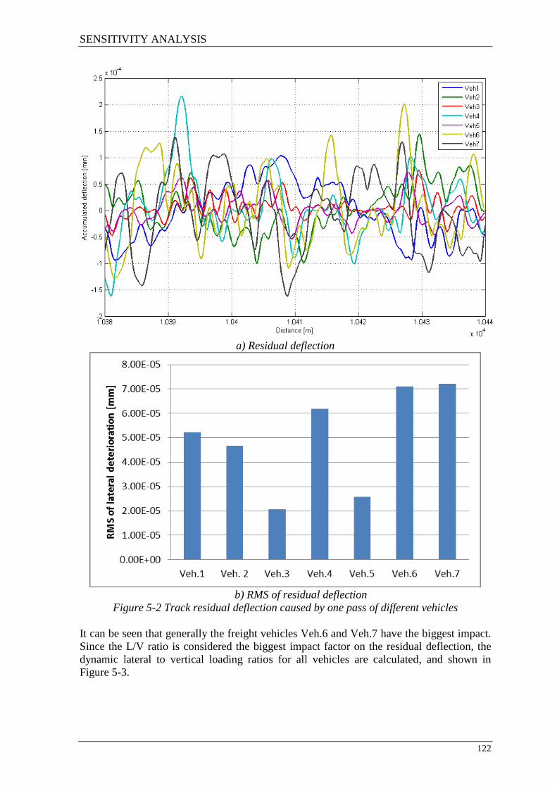
SENSITIVITY ANALYSIS
122
a) Residual deflection
b) RMS of residual deflection
Figure 5-2 Track residual deflection caused by one pass of different vehicles
It can be seen that generally the freight vehicles Veh.6 and Veh.7 have the biggest impact.
Since the L/V ratio is considered the biggest impact factor on the residual deflection, the
dynamic lateral to vertical loading ratios for all vehicles are calculated, and shown in
Figure 5-3.

SENSITIVITY ANALYSIS
123
a) Passenger vehicles
b) 4-axle freight vehicles
c) 2-axle freight vehicles
Figure 5-3 Lateral to vertical loading ratio delivered from vehicles to rail

SENSITIVITY ANALYSIS
124
Figure 5-4 is the summary of the average RMS of lateral forces and L/V ratio from
different vehicles. For the passenger vehicles Veh.1 to Veh.3, Veh.1 has the largest lateral
forces and L/V ratio while Veh.3 has the smallest. Therefore, the resulting residual
deflection caused by Veh.1 is the largest, as shown in Figure 5-2 b). On the other hand, the
laden freight vehicles have much smaller L/V ratios than tare, but create larger residual
deflections. The reason is that the laden vehicles have higher lateral forces. Therefore, it
can be deduced that the residual deflection depends on both the magnitude of the lateral
forces and the L/V loading ratio.
a) Average RMS of lateral force
b) Average RMS of lateral L/V ratio
Figure 5-4 Summary of average lateral forces and L/V ratio of different vehicles
Considering the dynamic forces experienced by each sleeper, the influence factors can be
determined. According to Chapter 4.3.3, the residual deflection under certain lateral and
vertical forces can be calculated as described in Figure 5-5. Therefore, the lateral residual
deflection can be calculated using Equation 64.

SENSITIVITY ANALYSIS
125
Equation 64
Substitute the values in Figure 5-5 into Equation 64 and rearranging gives:
(
) Equation 65
Figure 5-5 Residual deflection calculation
With the complicated vehicle-track dynamic interactions, it is difficult to solve the
equation and establish a simple equation for the force influence factor of the lateral
residual deflection. If the damping is not considered, the only influence factors are the L/V
loading ratio ( ⁄ ) and distributed lateral forces on the sleeper ( ).
(
)
(
⁄
)
Equation 66
For vehicles with similar lateral forces, the larger the L/V ratio becomes the larger the
residual deflection is. Meanwhile, vehicles with a similar L/V ratio, but larger lateral forces
result in a larger lateral residual deflection. For vehicles with different L/V ratios and
lateral forces, it is better to use the vehicle-track model to simulate the influences. For the
WCML data, the 2-axle vehicles give the largest residual deflection for each vehicle pass,
even though the speed limit for these vehicles is lower.

SENSITIVITY ANALYSIS
126
5.1.2 Effect of different running speed
The running speed of the vehicle has a significant influence on the vehicle-track dynamics,
and different types of vehicles have different speed limits. Veh.1 is chosen to investigate
how the running speed of the vehicle can influence the lateral residual deflection. The
speeds that will be considered are shown in Table 5-1. All the simulations are under 1000
vehicle passes.
Table 5-1 Different vehicle running speed mph m/s
-20% 80 35.763
-15% 85 37.998
-10% 90 40.234
-5% 95 42.469
Original 100.00 44.704
+5% 105 46.939
+10% 110 49.174
+15% 115 51.410
+20% 120 53.645
Figure 5-6 shows the resulting residual deflection for the different speeds mentioned above.
There is no obvious relationship that can be determined from these results.
Figure 5-6 Residual deflection at different speed
Figure 5-7 illustrates the peak residual deflections obtained from running the vehicle at
different speeds. No clear trend can be found for the peak residual deflection although the
maximum RMS of the residual deflection is the largest at 95 mph.

SENSITIVITY ANALYSIS
127
a) Peak residual deflections
b) RMS of residual deflections
Figure 5-7 Peak and average residual deflection at different speed
It is informative to examine the impact of speed on the residual deflection in the spatial
domain. Figure 5-8 and Table 5-2 summarise the lateral force PSD peak changes in spatial
domain.
Figure 5-8 PSD of residual deflections resulted by different speeds

SENSITIVITY ANALYSIS
128
Table 5-2 Summary of two peaks in PSD of residual deflections
Peak 1 Peak2
Fre
qu
ency
[cy
cle/
m]
Wa
vel
eng
th
[m]
Am
pli
tud
e
[mm
2/c
ycl
e/
m]
Fre
qu
ency
[cy
cle/
m]
Wa
vel
eng
th
[m]
Am
pli
tud
e
-20% 0.01953 51.2033 0.0687 0.1367 7.3153 0.01148
-15% 0.01953 51.2033 0.1376 0.1367 7.3153 0.01052
-10% 0.01953 51.2033 0.2040 0.1367 7.3153 0.00832
-5% 0.01953 51.2033 0.2263 0.1367 7.3153 0.00724
Original 0.01953 51.2033 0.2020 0.1367 7.3153 0.00479
+5% 0.01953 51.2033 0.1755 0.1367 7.3153 0.00651
+10% 0.01953 51.2033 0.1364 0.1367 7.3153 0.00926
+15% 0.01953 51.2033 0.0809 0.1367 7.3153 0.00752
+20% 0.01953 51.2033 0.0306 0.1367 7.3153 0.01149
It is found that the wavelengths of the first two peaks do not change, while the power
density of the residual deflection at these peaks does change. The 1st peak PSD change
agrees with the result of the average residual deflection change, while the 2nd
peak PSD has
the opposite trend. As the peak PSD of the 1st peak is much bigger than the 2
nd, the
influence of the 1st peak is much larger on the residual deflection.
a) Peak 1
b) Peak 2
Figure 5-9 Two peak power densities change

SENSITIVITY ANALYSIS
129
The change of the vehicle speed does not necessarily bring about a wavelength change in
the residual deflection, however, it creates small amplitude change to the track
deterioration. There will be a critical speed that creates the peak residual deflection and
reducing or increasing the vehicle speed, within permitted operational speed, can reduce
the residual deflection.
5.1.3 Effect of axle passages
The effect of the different vehicles on the residual deflection taking into account the actual
traffic mix by factoring the obtained residual deflection for one pass with the number of
axle passes is shown in Figure 5-10. It shows that Veh.1 has the major influence on the
lateral track irregularity growth compared to other vehicles. This is due to the fact that this
vehicle makes up more than 95% of the traffic on this section of the WCML, as shown in
in Table 5-3.
Figure 5-10 Residual deflection caused by different vehicles
Different vehicles have different dynamic behaviour thereby creating different lateral
damage to the track. From the results shown in Figure 5-2 a), Veh.2 appears to create a
lateral deterioration with a negative correlation to the deterioration created by Veh.1.
Interestingly, a different traffic mix can help to reduce the lateral deterioration created by
different vehicles. To illustrate this, the traffic pattern has been altered between Veh.1 and
Veh.2; the resulting changed D8 – D9 traffic is shown in the table below.
Table 5-3 Axle passages for each vehicle Veh.1 Veh.2 Veh.3 Veh.4 Veh.5 Veh.6 Veh.7
D8 – D9 19023 1416 346 1064 739 52 36
Changed D8 – D9 10219 10219 346 1064 739 52 36
Figure 5-11 shows the results of the track lateral deterioration under the actual and
optimised traffic scenario. It can be seen that the lateral deterioration created by Veh.1 is
almost opposite to the deterioration created by Veh.2, so more axle passages of Veh.2 can
effectively reduce the deterioration created by Veh.1. The SD of the track section drops to
0.4283 from 0.5476 by changing the traffic mix.

SENSITIVITY ANALYSIS
130
a) Actual traffic scenario (D8-D9)

SENSITIVITY ANALYSIS
131
b) Designed traffic scenario (Changed D8-D9)
Figure 5-11 Track deterioration under actual traffic and designed traffic scenario
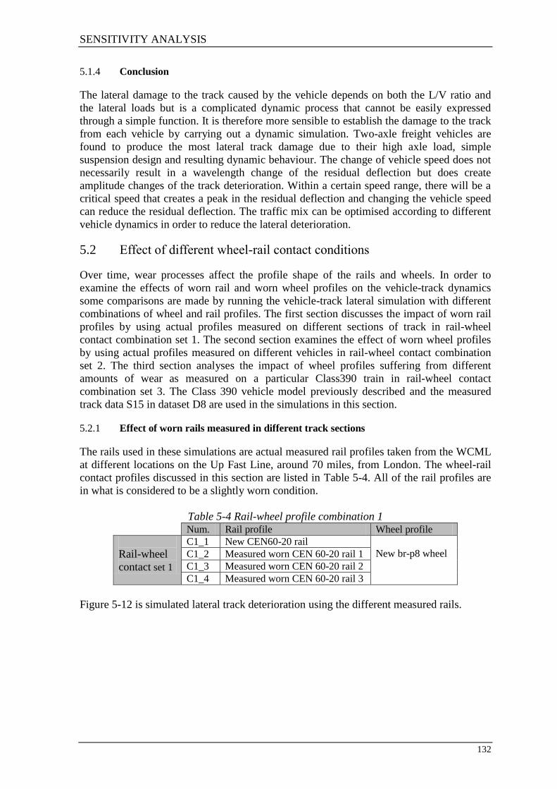
SENSITIVITY ANALYSIS
132
5.1.4 Conclusion
The lateral damage to the track caused by the vehicle depends on both the L/V ratio and
the lateral loads but is a complicated dynamic process that cannot be easily expressed
through a simple function. It is therefore more sensible to establish the damage to the track
from each vehicle by carrying out a dynamic simulation. Two-axle freight vehicles are
found to produce the most lateral track damage due to their high axle load, simple
suspension design and resulting dynamic behaviour. The change of vehicle speed does not
necessarily result in a wavelength change of the residual deflection but does create
amplitude changes of the track deterioration. Within a certain speed range, there will be a
critical speed that creates a peak in the residual deflection and changing the vehicle speed
can reduce the residual deflection. The traffic mix can be optimised according to different
vehicle dynamics in order to reduce the lateral deterioration.
5.2 Effect of different wheel-rail contact conditions
Over time, wear processes affect the profile shape of the rails and wheels. In order to
examine the effects of worn rail and worn wheel profiles on the vehicle-track dynamics
some comparisons are made by running the vehicle-track lateral simulation with different
combinations of wheel and rail profiles. The first section discusses the impact of worn rail
profiles by using actual profiles measured on different sections of track in rail-wheel
contact combination set 1. The second section examines the effect of worn wheel profiles
by using actual profiles measured on different vehicles in rail-wheel contact combination
set 2. The third section analyses the impact of wheel profiles suffering from different
amounts of wear as measured on a particular Class390 train in rail-wheel contact
combination set 3. The Class 390 vehicle model previously described and the measured
track data S15 in dataset D8 are used in the simulations in this section.
5.2.1 Effect of worn rails measured in different track sections
The rails used in these simulations are actual measured rail profiles taken from the WCML
at different locations on the Up Fast Line, around 70 miles, from London. The wheel-rail
contact profiles discussed in this section are listed in Table 5-4. All of the rail profiles are
in what is considered to be a slightly worn condition.
Table 5-4 Rail-wheel profile combination 1 Num. Rail profile Wheel profile
Rail-wheel
contact set 1
C1_1 New CEN60-20 rail
New br-p8 wheel C1_2 Measured worn CEN 60-20 rail 1
C1_3 Measured worn CEN 60-20 rail 2
C1_4 Measured worn CEN 60-20 rail 3
Figure 5-12 is simulated lateral track deterioration using the different measured rails.

SENSITIVITY ANALYSIS
133
Figure 5-12 Track lateral deterioration with different worn rails
The graph shows that while similar deterioration occurs at similar locations, the amplitude
of the deflection varies with different worn rail profiles. Small differences of rolling radius
difference due to rails in different wear condition can lead to very different dynamic lateral
forces, as shown in Figure 5-13.

SENSITIVITY ANALYSIS
134
a) Rolling radius difference all contact files
b) Leading left wheel lateral forces
Figure 5-13 Leading left wheel lateral forces with different rail profiles
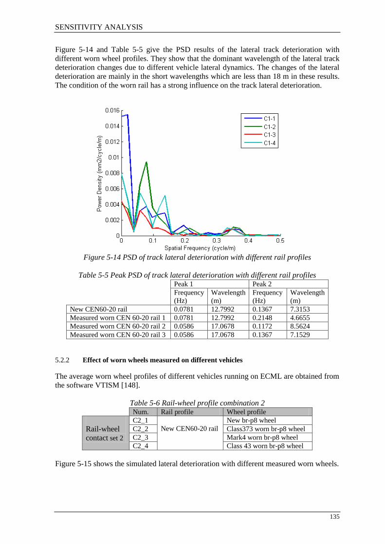
SENSITIVITY ANALYSIS
135
Figure 5-14 and Table 5-5 give the PSD results of the lateral track deterioration with
different worn wheel profiles. They show that the dominant wavelength of the lateral track
deterioration changes due to different vehicle lateral dynamics. The changes of the lateral
deterioration are mainly in the short wavelengths which are less than 18 m in these results.
The condition of the worn rail has a strong influence on the track lateral deterioration.
Figure 5-14 PSD of track lateral deterioration with different rail profiles
Table 5-5 Peak PSD of track lateral deterioration with different rail profiles Peak 1 Peak 2
Frequency
(Hz)
Wavelength
(m)
Frequency
(Hz)
Wavelength
(m)
New CEN60-20 rail 0.0781 12.7992 0.1367 7.3153
Measured worn CEN 60-20 rail 1 0.0781 12.7992 0.2148 4.6655
Measured worn CEN 60-20 rail 2 0.0586 17.0678 0.1172 8.5624
Measured worn CEN 60-20 rail 3 0.0586 17.0678 0.1367 7.1529
5.2.2 Effect of worn wheels measured on different vehicles
The average worn wheel profiles of different vehicles running on ECML are obtained from
the software VTISM [148].
Table 5-6 Rail-wheel profile combination 2 Num. Rail profile Wheel profile
Rail-wheel
contact set 2
C2_1
New CEN60-20 rail
New br-p8 wheel
C2_2 Class373 worn br-p8 wheel
C2_3 Mark4 worn br-p8 wheel
C2_4 Class 43 worn br-p8 wheel
Figure 5-15 shows the simulated lateral deterioration with different measured worn wheels.

SENSITIVITY ANALYSIS
136
Figure 5-15 Track lateral deterioration with different worn wheels
The results are different from each other mainly due to the vehicle lateral dynamic
behaviour changing with the different contact conditions, as shown in Figure 5-16.
a) Rolling radius difference for all contact files
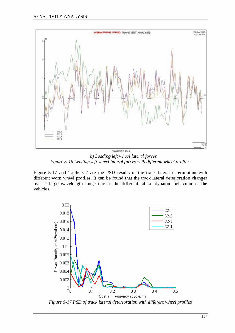
SENSITIVITY ANALYSIS
137
b) Leading left wheel lateral forces
Figure 5-16 Leading left wheel lateral forces with different wheel profiles
Figure 5-17 and Table 5-7 are the PSD results of the track lateral deterioration with
different worn wheel profiles. It can be found that the track lateral deterioration changes
over a large wavelength range due to the different lateral dynamic behaviour of the
vehicles.
Figure 5-17 PSD of track lateral deterioration with different wheel profiles

SENSITIVITY ANALYSIS
138
Table 5-7 Peak PSD of track lateral deterioration with different wheel profiles Peak 1 Peak 2
Frequency
(Hz)
Wavelength
(m)
Frequency
(Hz)
Wavelength
(m)
New BR-P8 wheel 0.0781 12.7992 0.1367 7.3153
Class373 worn BR-P8 wheel 0.0195 51.2033 0.1367 7.3153
Mark4 worn BR-P8 wheel 0.0781 12.7992 0.1367 7.3153
Class43 worn BR-P8 wheel 0.0586 17.0678 0.1367 7.3153
5.2.3 Effect of different level of worn wheels
A conclusion can be drawn from section 5.2.1 and section 5.2.2 that the wheel-rail contact
condition makes a significant difference to the vehicle lateral dynamics, and hence the
lateral track deterioration. In reality, wheels tend to wear differently, and there may be
different amounts of wear occurring on the different wheels of a train. Therefore, it is
necessary to examine how different levels of wear affect the lateral deterioration. The worn
wheel profiles used in this section were measured on one Class390 train.
Table 5-8 Rail-wheel profile combination 3 Num. Rail profile Wheel profile
Rail-wheel
contact set 3
C3_1
Measured worn CEN
60-20 rail 1
Class390 worn br-p8 wheel 1
C3_2 Class390 worn br-p8 wheel 2
C3_3 Class390 worn br-p8 wheel 3
C3_4 Class390 worn br-p8 wheel 4
C3_5 Class390 worn br-p8 wheel 5
* 1 to 5 indicates increasing wear
Figure 5-18 is the simulated lateral track deterioration for different levels of wheel wear. It
is clear that different worn profiles have a large impact on lateral track deterioration.
Figure 5-18 Track lateral deterioration with different level of worn wheels

SENSITIVITY ANALYSIS
139
Figure 5-19 is the rolling radius difference and the dynamic lateral forces of the leading
left wheel for all of the wheel-rail contact profiles. Vehicles have very different lateral
behaviours under different wear conditions.
a) Rolling radius difference of five contact files
b) Leading left wheel lateral forces
Figure 5-19 Rolling radius difference of five contact files

SENSITIVITY ANALYSIS
140
Figure 5-20 and Table 5-9 are the PSD results of the lateral track deterioration with
different worn wheel profiles. It shows that if the wheel is seriously worn, the conicity
between the wheel and rail reduces. This leads to a decrease in the long wavelength lateral
deterioration at around 50 m. When the wheel is worn into different shapes as for example
C2-2 and C3-3, the vehicle lateral dynamics can change significantly. It is noted that with
the most worn wheel profiles, as in C3-4 and C3-5, there is a noticeable drop in the lateral
track deterioration.
a) PSD
b) RMS
Figure 5-20 PSD and RMS of track lateral deterioration with different level of worn wheel
profiles

SENSITIVITY ANALYSIS
141
Table 5-9 Peak PSD of track lateral deterioration with different level of worn wheel
profiles Peak 1 Peak 2
Frequency
(Hz)
Wavelength
(m)
Frequency
(Hz)
Wavelength
(m)
C3_1 0.0195 51.2033 0.0781 12.7992
C3_2 0.0195 51.2033 0.1367 7.3153
C3_3 0.0195 51.2033 0.1367 7.3153
C3_4 0.0195 51.2033 0.1367 7.3153
C3_5 0.1367 7.3153 0.1953 5.1203
In general, as the wheels wear, there is a general trend for the conicity to reduce leading to
lower lateral forces and reduced track damage. This result on a curve maybe different as
the reduced steering can also lead to large dynamic forces due to flange contact. However,
the life of railway wheels is usually limited by wear, and the wear between rail and wheel
can lead to problems in stability, increased life cycle cost and passenger discomfort. This
results in a conflict between the optimum worn rail and wheel profile for lateral track
deterioration and for other aspects.
5.2.4 Conclusion
It was found that the wheel and rail profiles play a very important role in the track lateral
deterioration by influencing the vehicle-track lateral dynamics. Different worn rail and
wheel profiles lead to significantly different lateral dynamic forces for the vehicle. For a
fixed worn rail and variations in wheel wear on a particular type of vehicle, the increase in
wheel wear tends to reduce the lateral track deflection due to a reduction in both conicity
and lateral forces. Therefore, it is important to select correct wheel and rail profiles, and
find representative wheel-rail contact data for the track section that needs to be analysed. A
better understanding of rail-wheel wear can lead to a more accurate prediction.
5.3 Effects of different track parameters
The influence of track parameters on lateral track deterioration is investigated in this
section. The Class390 model Veh.1, is chosen to run over track section 1 in Section 4.5 as
it is the predominant vehicle operating on this section. Due to the small effect one vehicle
pass will have on the lateral track alignment, 1000 passes of the vehicle will be simulated.
The method is to change one of the track parameters and then run simulations in order to
assess the sensitivity of the lateral track deterioration to this parameter. The original
parameters used in the analysis are shown in Table 5-10.
Table 5-10 Original parameters
N.s/m
N∙s/m
kg 60
kg 308
mm 0.03
kN 0.12

SENSITIVITY ANALYSIS
142
Due to the highly non-linear characteristics of the model, the change of the parameters may
introduce dynamic impacts into the results. Therefore, clear regular patterns can be found
in the results with some small exceptions.
5.3.1 Effects of track stiffness
Track stiffness has a big influence on the forces that are distributed from the rails to the
sleeper. Additionally, the stiffness values have an impact on sleeper-ballast pre-sliding
behaviour. Table 5-11 shows the stiffness values that are used in the following study. Each
stiffness value is varied from 80% to 120% of the original value one at a time. As the
sleeper-ballast lateral stiffness changes dynamically depending on the vertical load, the
variation of this value is achieved by altering the elastic breaking displacement, as shown
in the table.
Table 5-11 Stiffness variation
Rail-
sleeper
vertical
stiffness
Rail-
sleeper
lateral
stiffness
Sleeper-
ballast
vertical
stiffness
Sleeper-ballast
lateral stiffness
kN/mm [mm]
-20% 50.40 31.84 72.00
0.625
-15% 53.55 33.83 76.50
0.588
-10% 56.70 35.82 81.00
0.556
-5% 59.85 37.81 85.50
0.526
Original 63.00 39.80 90.00 0.500
+5% 66.15 41.79 94.50
0.476
+10% 69.30 43.78 99.00
0.454
+15% 72.45 45.77 103.50
0.434
+20% 75.60 47.76 108.00
0.417
The resulting accumulated track lateral deterioration is shown in Figure 5-21. It is found
that the shape of the residual deflection does not change and the amplitude changes by a
small amount.
kN 8.9
- 0.9986
- 0.01
- 0.045

SENSITIVITY ANALYSIS
143
Figure 5-21 Track lateral deflection with different rail-sleeper vertical stiffness values
The peak and RMS of the accumulated lateral deflection values with respect to all stiffness
changes are summarised in Table 5-12. Although the dynamic lateral sleeper-ballast
stiffness changes with the vertical distributed load, the dynamic stiffness varies around 18
kN/mm. This 18 kN/mm value is mainly defined by the static vertical forces due to vehicle
weight, and the variations are dependent on the dynamic vertical force variations which are
much smaller. It is therefore sensible to approximate the average change of the
deterioration per unit change of lateral sleeper-ballast stiffness according to this 18 kN/mm
value.
Table 5-12 Peak residual deflection under different rail-sleeper vertical stiffness
Peak deflection RMS of deflection
Unit [mm]
-20% 0.15234 0.15272 0.15230 0.16379 0.07433 0.07461 0.07427 0.07584
-15% 0.15236 0.15263 0.15233 0.15544 0.07422 0.07440 0.07416 0.07500
-10% 0.15238 0.15255 0.15236 0.15320 0.07425 0.07426 0.07422 0.07466
-5% 0.15239 0.15251 0.15238 0.15274 0.07428 0.07421 0.07427 0.07418
Original 0.15240 0.15240 0.15240 0.15240 0.07427 0.07427 0.07427 0.07427
+5% 0.15241 0.15210 0.15242 0.15243 0.07423 0.07411 0.07419 0.07421
+10% 0.15242 0.15194 0.15244 0.15225 0.07424 0.07386 0.07409 0.07421
+15% 0.15243 0.15188 0.15251 0.15153 0.07413 0.07378 0.07412 0.07406
+20% 0.15250 0.15182 0.15251 0.15136 0.07408 0.07345 0.07408 0.07398
Average
( ) 1.93 -11.2 2.53
-156 -3.21 -14.46 -2.39 -23.31
per unit
mm/kN/mm
( )
0.61
-5.63
0.56
-173
-1.02
-7.27
-0.53
-25.90
In % 0.0127 -0.0735 0.0166 -1.0202 -0.0432 -0.1948 -0.0322 -0.3139 * ‘Average ’ – the average change of the residual deflection for each 5% change of the stiffness
* ‘ per unit’ – the average per 1 kN/mm change of the stiffness.
* ‘In %’ – the proportion average takes of the original residual deflection value
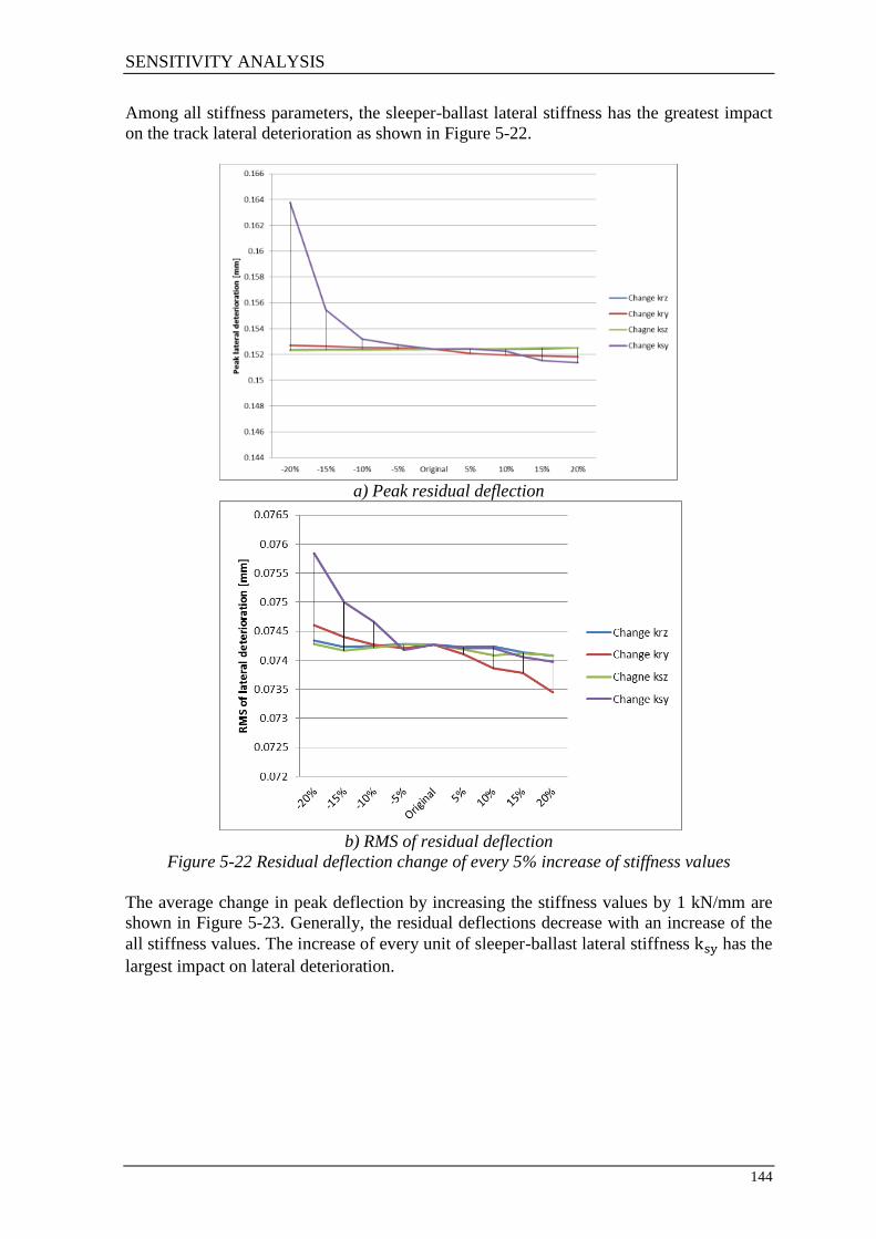
SENSITIVITY ANALYSIS
144
Among all stiffness parameters, the sleeper-ballast lateral stiffness has the greatest impact
on the track lateral deterioration as shown in Figure 5-22.
a) Peak residual deflection
b) RMS of residual deflection
Figure 5-22 Residual deflection change of every 5% increase of stiffness values
The average change in peak deflection by increasing the stiffness values by 1 kN/mm are
shown in Figure 5-23. Generally, the residual deflections decrease with an increase of the
all stiffness values. The increase of every unit of sleeper-ballast lateral stiffness has the
largest impact on lateral deterioration.

SENSITIVITY ANALYSIS
145
Figure 5-23 Average change per unit increase of stiffness value
5.3.2 Effects of track damping
Table 5-13 shows the rail-sleeper and sleeper-ballast damping values that are used in the
following simulations. Each damping value is varied between 80% and 120% of the
original value.
Table 5-13 Damping variation [kN.s/m]
Rail-
sleeper
vertical
damping
Rail-
sleeper
lateral
damping
Sleeper-
ballast
vertical
damping
Sleeper-
ballast
lateral
damping
-20% 32.0 24.0 64.0 24.0
-15% 34.0 25.5 68.0 25.5
-10% 36.0 27.0 72.0 27.0
-5% 38.0 28.5 76.0 28.5
Original 40.0 30.0 80.0 30.0
+5% 42.0 31.5 84.0 31.5
+10% 44.0 33.0 88.0 33.0
+15% 46.0 34.5 92.0 34.5
+20% 48.0 36.0 96.0 36.0
The lateral track deterioration results are shown in Figure 5-24. The differences between
all of the results are small when changing damping values.

SENSITIVITY ANALYSIS
146
Figure 5-24 Track lateral deflection with different rail-sleeper vertical damping values
The peak and RMS of the accumulated lateral deflection values are summarised in Table
5-14. Generally, it can be found that the residual deflection decreases with an increase of
all damping values.
Table 5-14 Peak residual deflection under different damping values
Peak deflection RMS of deflection
Unit [mm]
-20% 0.15241 0.15260 0.15243 0.15654 0.07426 0.07425 0.07426 0.07642
-15% 0.15241 0.15253 0.15242 0.15544 0.07426 0.07418 0.07427 0.07558
-10% 0.15240 0.15248 0.15242 0.15428 0.07426 0.07418 0.07426 0.07520
-5% 0.15240 0.15244 0.15241 0.15313 0.07426 0.07426 0.07426 0.07460
Original 0.15240 0.15240 0.15240 0.15240 0.07427 0.07427 0.07427 0.07427
+5% 0.15240 0.15236 0.15239 0.15133 0.07427 0.07424 0.07427 0.07347
+10% 0.15240 0.15238 0.15239 0.15016 0.07427 0.07418 0.07427 0.07289
+15% 0.15240 0.15253 0.15238 0.14900 0.07427 0.07423 0.07423 0.07227
+20% 0.15239 0.15249 0.15237 0.14787 0.07427 0.07422 0.07420 0.07173
Average
( ) -0.19 -1.35 -0.78 -108.37 0.01 -0.32 -0.76 -58.56
In
mm/kN.s/
mm
( )
-0.09
-0.90
-0.20
-72.25
0.01
-0.22
-0.19
-39.04
In % -0.0012 -0.0089 -0.0051 -0.7111 0.0002 -0.0044 -0.0102 -0.7886
Among all of the damping parameters, the sleeper-ballast lateral damping has the greatest
impact on lateral track deterioration.

SENSITIVITY ANALYSIS
147
a) Peak residual deflection
b) RMS of residual deflection
Figure 5-25 Residual deflection change for every 5% increase of damping values
In general, the lateral residual deflection tends to reduce with the growth of all damping
values. The change in sleeper-ballast damping value , has the largest impact on lateral
deterioration. Other damping values have negligible effect.
Figure 5-26 Average change per unit increase of damping value

SENSITIVITY ANALYSIS
148
5.3.3 Effect of rail and sleeper mass
Rail and sleeper mass have a direct influence on the unloading condition shown in Figure
4-23. The unloading of the track creates a low resistance to lateral deterioration. Table 5-15
shows the rail and sleeper masses that are used in the following study. Each mass is varied
from 80% to 120% of the original mass values.
Table 5-15 Rail and sleeper masses variation [kg]
-20% 48 246.4
-15% 51 261.8
-10% 54 277.2
-5% 57 292.6
Original 60 308
+5% 63 323.4
+10% 66 338.8
+15% 69 354.2
+20% 72 369.6
The resulting lateral track deterioration is shown in Figure 5-27.
Figure 5-27 Track lateral deflection with different rail and sleeper masses
The peak and RMS of the accumulated lateral deflection values with respect to rail and
sleeper mass changes are summarised in Table 5-14.
Table 5-16 Peak residual deflection under different rail and sleeper masses [mm]
Peak deflection RMS of deflection
Unit [mm]
-20% 0.15603 0.17542 0.07510 0.08558
-15% 0.15517 0.16686 0.07485 0.08223
-10% 0.15432 0.16187 0.07467 0.07951
-5% 0.15350 0.15744 0.07436 0.07659
Original 0.15240 0.15240 0.07427 0.07427
+5% 0.15161 0.14802 0.07390 0.07209
+10% 0.15075 0.14423 0.07357 0.07001

SENSITIVITY ANALYSIS
149
+15% 0.15005 0.14935 0.07342 0.06823
+20% 0.14937 0.14691 0.07314 0.06668
Average
( ) -83.32 -356.44 -24.52 -236.29
In mm/kg
( )
-27.77
-23.15 -8.17 -15.34
In % -0.5467 -2.3388 -0.3301 -3.1816
It is found that the residual deflection decreases with every 5% increase of both rail and
sleeper masses. The sleeper mass has the largest effect.
a) Peak residual deflection
b) RMS of residual deflection
Figure 5-28 Residual deflection amplitude change of every 5% increase of masses

SENSITIVITY ANALYSIS
150
Figure 5-29 shows that for every kilogram that the sleeper mass increase leads to a
further decrease of the lateral track deterioration.
Figure 5-29 Average change per unit increase of rail and sleeper masses
5.3.4 Effect of softening factor
The softening factor depends on the condition of the sleeper-ballast interface, and track in
good condition has a softening factor close to 1. A variation in alters the hysteresis
characteristic and indicates a more gentle stiffness for residual deflection calculation. As a
result, a reduction in leads to an increase in residual deflection as shown in Figure 5-30.
Figure 5-30 Change of softening factor
The stiffness for residual deflection must be less than the elastic stiffness, therefore the
softening factor value needs to be smaller than 1. Table 5-17 is the softening factor that is
used in this section.

SENSITIVITY ANALYSIS
151
Table 5-17 Softening factor variation
-2.0% 0.9604
-1.5% 0.9653
-1.0% 0.9702
-0.5% 0.9751
Original 0.9800
+0.5% 0.9849
+1.0% 0.9898
+1.5% 0.9947
+2.0% 0.9996
The simulated lateral track deterioration using different softening factors is shown in
Figure 5-30.
Figure 5-31 Track lateral deflection with softening factors
The peak and RMS of the accumulated lateral deflection values with respect to different
softening factors are summarised in Table 5-18.
Table 5-18 Peak residual deflection under different softening factors [mm]
Peak deflection RMS of deflection
Unit [mm]
-2.0% 4.25319 1.73421
-1.5% 3.72427 1.51853
-1.0% 3.19609 1.30315
-0.5% 2.66867 1.08809
Original 2.14199 0.87334
+0.5% 1.61606 0.65890
+1.0% 1.09087 0.44476
+1.5% 0.56643 0.23094
+2.0% 0.04272 0.01742
Average -0.52631 -0.21460 In % -24.5710 -24.5722

SENSITIVITY ANALYSIS
152
The change of softening factor only brings an amplitude change to the residual deflection.
The impact of this parameter on the residual deflection is linear, and for every 0.5%
increase of this value causes a 24.5% reduction in the lateral residual deflection.
a) Peak residual deflection
b) RMS of residual deflection
Figure 5-32 Residual deflection change of every 0.5% increase in softening factor
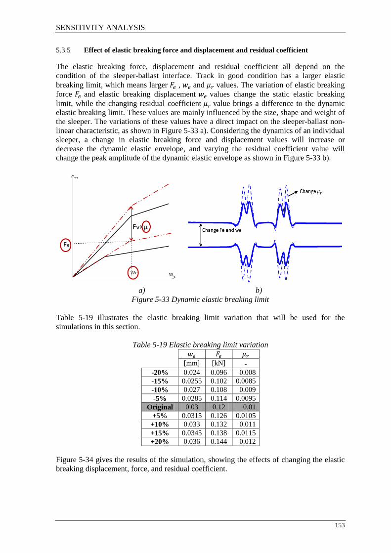
SENSITIVITY ANALYSIS
153
5.3.5 Effect of elastic breaking force and displacement and residual coefficient
The elastic breaking force, displacement and residual coefficient all depend on the
condition of the sleeper-ballast interface. Track in good condition has a larger elastic
breaking limit, which means larger , and values. The variation of elastic breaking
force and elastic breaking displacement values change the static elastic breaking
limit, while the changing residual coefficient value brings a difference to the dynamic
elastic breaking limit. These values are mainly influenced by the size, shape and weight of
the sleeper. The variations of these values have a direct impact on the sleeper-ballast non-
linear characteristic, as shown in Figure 5-33 a). Considering the dynamics of an individual
sleeper, a change in elastic breaking force and displacement values will increase or
decrease the dynamic elastic envelope, and varying the residual coefficient value will
change the peak amplitude of the dynamic elastic envelope as shown in Figure 5-33 b).
a) b)
Figure 5-33 Dynamic elastic breaking limit
Table 5-19 illustrates the elastic breaking limit variation that will be used for the
simulations in this section.
Table 5-19 Elastic breaking limit variation
[mm] [kN] -
-20% 0.024 0.096 0.008
-15% 0.0255 0.102 0.0085
-10% 0.027 0.108 0.009
-5% 0.0285 0.114 0.0095
Original 0.03 0.12 0.01
+5% 0.0315 0.126 0.0105
+10% 0.033 0.132 0.011
+15% 0.0345 0.138 0.0115
+20% 0.036 0.144 0.012
Figure 5-34 gives the results of the simulation, showing the effects of changing the elastic
breaking displacement, force, and residual coefficient.
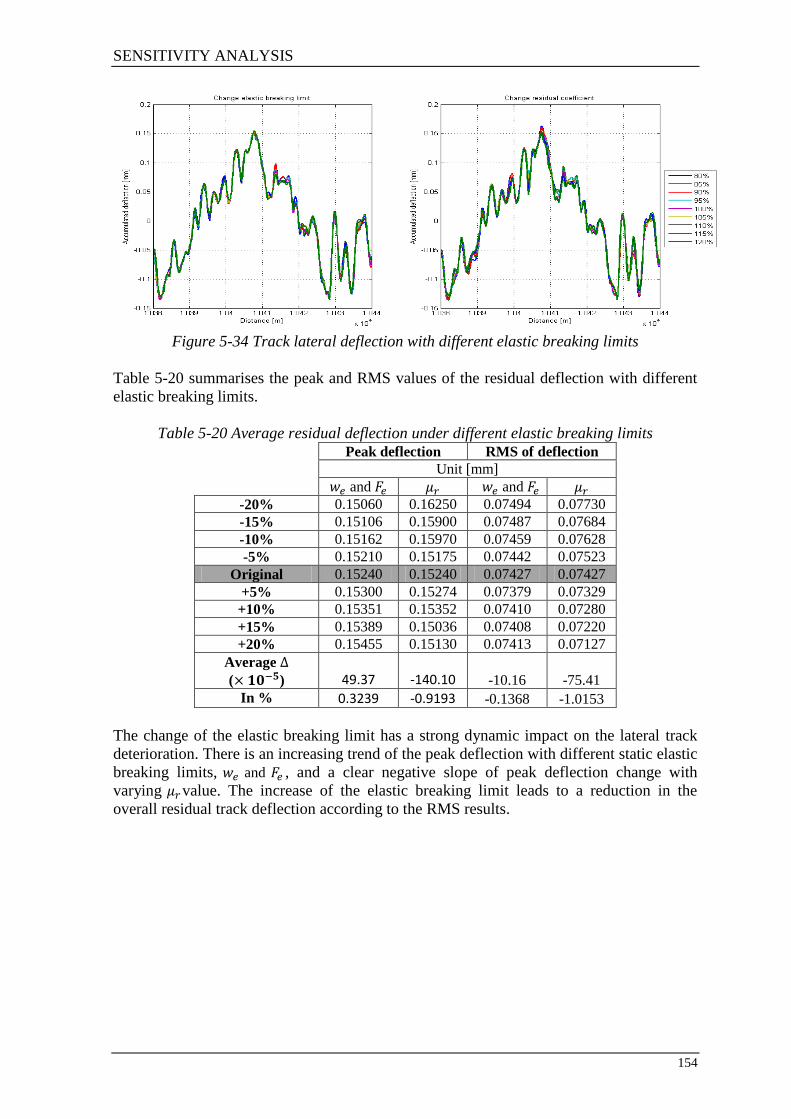
SENSITIVITY ANALYSIS
154
Figure 5-34 Track lateral deflection with different elastic breaking limits
Table 5-20 summarises the peak and RMS values of the residual deflection with different
elastic breaking limits.
Table 5-20 Average residual deflection under different elastic breaking limits
Peak deflection RMS of deflection
Unit [mm]
and and -20% 0.15060 0.16250 0.07494 0.07730
-15% 0.15106 0.15900 0.07487 0.07684
-10% 0.15162 0.15970 0.07459 0.07628
-5% 0.15210 0.15175 0.07442 0.07523
Original 0.15240 0.15240 0.07427 0.07427
+5% 0.15300 0.15274 0.07379 0.07329
+10% 0.15351 0.15352 0.07410 0.07280
+15% 0.15389 0.15036 0.07408 0.07220
+20% 0.15455 0.15130 0.07413 0.07127
Average
( ) 49.37 -140.10 -10.16 -75.41
In % 0.3239 -0.9193 -0.1368 -1.0153
The change of the elastic breaking limit has a strong dynamic impact on the lateral track
deterioration. There is an increasing trend of the peak deflection with different static elastic
breaking limits, and , and a clear negative slope of peak deflection change with
varying value. The increase of the elastic breaking limit leads to a reduction in the
overall residual track deflection according to the RMS results.

SENSITIVITY ANALYSIS
155
a) Peak residual deflection
b) RMS of residual deflection
Figure 5-35 Residual deflection change by elastic breaking limits
5.3.6 Effect of sleeper spacing
Changing the sleeper spacing changes the supporting condition of the rails, so it can
influence the track lateral dynamics. The sleeper spacing values simulated in this section
are shown in Table 5-21.
Table 5-21 Sleeper spacing variation [m]
Sleeper spacing
-20% 0.48
-15% 0.51
-10% 0.54
-5% 0.57
Original 0.6
+5% 0.63
+10% 0.66
+15% 0.69
+20% 0.72
The resulting lateral track deteriorations with different sleeper spacing values are shown in
Figure 5-36.
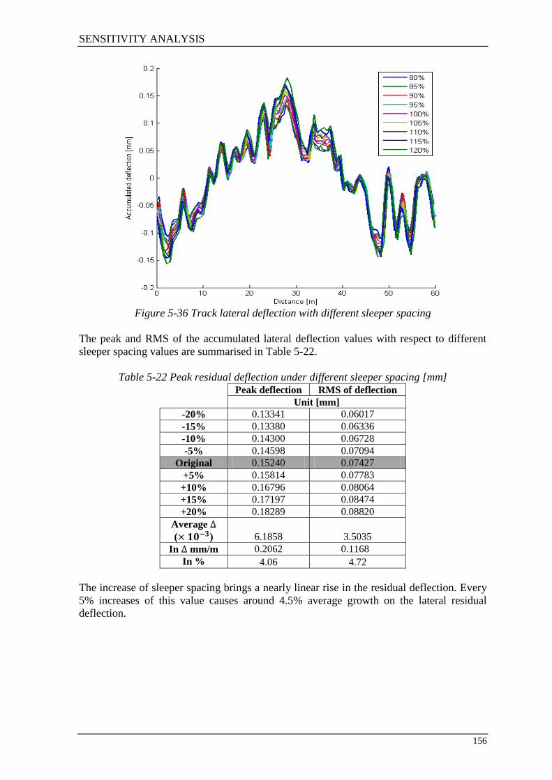
SENSITIVITY ANALYSIS
156
Figure 5-36 Track lateral deflection with different sleeper spacing
The peak and RMS of the accumulated lateral deflection values with respect to different
sleeper spacing values are summarised in Table 5-22.
Table 5-22 Peak residual deflection under different sleeper spacing [mm]
Peak deflection RMS of deflection
Unit [mm]
-20% 0.13341 0.06017
-15% 0.13380 0.06336
-10% 0.14300 0.06728
-5% 0.14598 0.07094
Original 0.15240 0.07427
+5% 0.15814 0.07783
+10% 0.16796 0.08064
+15% 0.17197 0.08474
+20% 0.18289 0.08820
Average
( ) 6.1858 3.5035
In mm/m 0.2062 0.1168
In % 4.06 4.72
The increase of sleeper spacing brings a nearly linear rise in the residual deflection. Every
5% increases of this value causes around 4.5% average growth on the lateral residual
deflection.
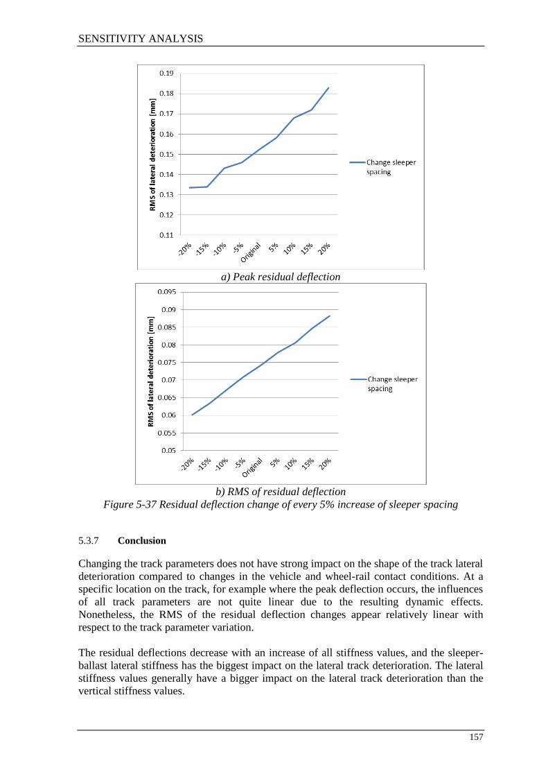
SENSITIVITY ANALYSIS
157
a) Peak residual deflection
b) RMS of residual deflection
Figure 5-37 Residual deflection change of every 5% increase of sleeper spacing
5.3.7 Conclusion
Changing the track parameters does not have strong impact on the shape of the track lateral
deterioration compared to changes in the vehicle and wheel-rail contact conditions. At a
specific location on the track, for example where the peak deflection occurs, the influences
of all track parameters are not quite linear due to the resulting dynamic effects.
Nonetheless, the RMS of the residual deflection changes appear relatively linear with
respect to the track parameter variation.
The residual deflections decrease with an increase of all stiffness values, and the sleeper-
ballast lateral stiffness has the biggest impact on the lateral track deterioration. The lateral
stiffness values generally have a bigger impact on the lateral track deterioration than the
vertical stiffness values.

SENSITIVITY ANALYSIS
158
Track deterioration decreases as damping values increase, and the sleeper-ballast damping
in the lateral direction is found to have the biggest influence.
The increase in mass of both rails and sleepers leads to a reduction of the lateral track
deflection, and changes of sleeper mass have a greater effect than changes in the mass of
the rails.
Increasing of the softening factor in the ballast-sleeper interface model creates amplitude
reduction in the lateral track deterioration. The relationship between the softening factor
and track deterioration is linear.
The impact of the elastic breaking limits, which are determined by the elastic breaking
force, displacement and residual coefficient, is discussed. An increase in the elastic
breaking limit, which means a stronger lateral sleeper-ballast interface, leads to an
amplitude reduction in the overall track residual deflection.
An increase in sleeper spacing weakens the track support condition to some degree,
thereby leading to a potential growth in track lateral deterioration.
As expected, the sleeper-ballast interface has the biggest impact on the lateral track
deterioration since the parameters related to this interface all appear to have the greatest
impact on lateral deterioration.
5.4 Chapter conclusion
This chapter presented the influences of different aspects on the lateral track deterioration
in terms of the vehicles, wheel-rail contact conditions and track parameters.
The lateral damage caused by the vehicle depends on both the L/V ratio and the lateral load
but it is a complicated dynamic process that cannot easily be expressed through a simple
function. It is therefore sensible to establish the damage from different types of vehicle by
carrying out vehicle-track dynamic simulations. Two-axle freight vehicles were found to
produce most lateral track damage due to their high axle load, simple suspension design
and resulting dynamic behaviour. The change of vehicle speed does not necessarily bring a
wavelength change of the residual deflection but does cause a change to the amplitude of
the track deterioration. Within a certain speed range, there will be a critical speed that
creates a peak in the residual deflection, and reducing or increasing the vehicle speed can
help reduce the residual deflection.
It is found that the wheel and rail profiles play a very important role in the development of
lateral track deterioration by influencing the lateral dynamics of the vehicle. Different
worn rail and wheel profiles result in very different lateral dynamic forces. For a fixed
worn rail and worn wheel on a particular type of vehicle, the increase in wheel wear can
make the residual track deflection lower due to reduced conicity and lateral forces. It is
important to choose the correct wheel and rail profiles, and find representative wheel-rail
contact conditions for the track section that is being analysed. A better understanding of
rail-wheel wear can lead to a more accurate prediction.

SENSITIVITY ANALYSIS
159
The sleeper-ballast interface is found to have the biggest impact on the lateral track
deterioration since the parameters related to this interface all have the strongest impact on
the lateral deterioration. The change of track parameters does not have a large impact on
the shape of the lateral track deterioration compared to the vehicle and wheel-rail contact
changes. At the specific location on the track where the peak deflection occurs, the
influences by all different track parameters are not quite linear due to the resulting dynamic
effects. Nevertheless, the RMS of the residual deflection changes appear relatively linear
with respect to the track parameter variation. The changes in track lateral deterioration with
respect to various changing parameters are listed below:
The residual deflections decrease with an increase of all stiffness and damping
values, and the sleeper-ballast lateral stiffness and damping have the largest impact
on lateral track deterioration.
An increase of rail and sleeper mass gives a reduction in the lateral track residual
deflection, and for every kilogram increase in sleeper mass, a reduction in the
residual deflection is seen that is greater than that for a similar change in the mass
of the rails.
Increasing the softening factor gives a linear amplitude reduction of the lateral track
deterioration.
An increase of the elastic breaking limit in the model leads to an amplitude
reduction of the residual track deflection.
If the sleeper spacing increases, the lateral track deterioration will also increase.

FURTHER WORK AND RECOMMENDATIONS
160
6 FURTHER WORK AND RECOMMENDATIONS
The mechanism of railway track lateral deterioration has been studied through statistical
analysis and modelling processes. Scenarios that have not been attempted are discussed
here as potential further research subjects. Points for further development of the vehicle-
track lateral deterioration model are given in order to improve the accuracy, speed and
applicability of the model.
6.1 Further work
6.1.1 Extension of statistical analysis
It was shown that the track lateral and vertical irregularities are correlated to some extent
in both the distance domain and spatial domain. On average the lateral quality is slightly
better than the vertical, however there are cases where it can be significantly worse. Due to
the limitation of the recorded track data, the lateral track deterioration against the curvature
and time are studied separately, so the parameters for these empirical functions are only
valid on specific networks. The growth in the standard deviation of the lateral track
irregularity against track curvature has only been validated using the DynoTrain track data,
and the growth of the track lateral irregularity SD against time is only validated using a
particular section of WCML track data. Further work will be useful to create a more
comprehensive equation by combining the curvature and time (or loading cycles) factors,
and in addition, the factors that have not been included in this study, such as temperature,
ground condition, and traffic etc. To achieve this, additional analysis using measured track
data that includes all of the information mentioned above will be required.
6.1.2 Extension of parameters study
The track parameters in the lateral direction are not well understood, and previous research
in this area is quite limited. This is probably due to the difficulty of measuring these
parameters and the highly non-linear characteristics of lateral track behaviour. More
laboratory or field tests should be carried out to examine the track lateral stiffness and
damping values thereby making future research more accurate.
The sleeper-ballast interface failure has been studied in detail by Le Pen [72, 77]. However,
the lateral pre-sliding characteristics of the sleeper-ballast interface is not well understood,
in terms of the hysteresis features or the force-displacement characteristics. An in-depth
study of the pre-sliding characteristics would provide a better understanding and more
accurate parameters for future research.
6.1.3 Extension of model capabilities
The development of the model, presented in Chapter 4, potentially forms the basis for
further work to be carried out on each sub-system in the model. The validation results
predict a short wavelength deterioration that is not seen in the actual track deterioration. It
will be useful to understand the reason for the existence of this additional prediction, and
under what conditions it can be filtered out. The discussion below may explain the reason
for this behaviour.

FURTHER WORK AND RECOMMENDATIONS
161
For the vehicle dynamic model using VAMPIRE® software, efforts can be made to
improve the vehicle models to describe the actual vehicle suspension system better such as
the tilting mechanism of Class390, and be more representative of the exact vehicle type
running on a specific track section
The track model can be improved and modified in two different ways. One is to develop a
more comprehensive and complex model including additional key parameters, and the
other is to simplify certain aspects of the model and thus create a faster model that
describes the basic concept of lateral track deterioration. Both are discussed in more detail
below:
1. More complex model including additional key parameters
There are a few factors that were not considered in the model and including these
factors can make the model better at describing the complex dynamic behaviour of
the actual track system. However, this leads to a more complicated and time
consuming model. The potential factors that can be included in further development,
as well as their advantages and drawbacks, are listed below:
o Add longitudinal dynamics to the model, so for each rail node there will be
6 DOF instead of 4, and for sleeper nodes there will be 3 DOF instead of 2.
In this way, the influences of the longitudinal forces from the wheels to the
track system will be included as presented in Figure 2-8. This may increase
the calculation time significantly.
o The track data used in this research was collected between March and
September for which the temperature change does not cover all variation
expected over one year time. When the temperature changes through a
significant range, it creates thermal expansion and contraction of the rails. It
can be worthwhile to include the temperature influence on lateral track
deterioration at some locations.
o The track bed, including ballast, sub-ballast and capping layers are
considered as one track bed layer sitting on a rigid surface. This track bed
layer can be modelled in detail in terms of ballast layer, sub-ballast layer,
geotextile layer and subgrade. The change brought about by adding these
layers on the lateral deterioration results are unknown and may be worth
investigating, although there may be a chance that there will be no influence
resulting from these changes.
o The sleeper-ballast elastic and hysteresis characteristics are simplified into
two sections of linear force-displacement relationships. This non-linear
characteristic can be improved to a curve that is closer to the condition in
reality. The numerical calculation of this calculation can be solved using
many different methods, such as: Newton-Raphson method, displacement
control method, the constant work method and the minimum residual
displacement method.

FURTHER WORK AND RECOMMENDATIONS
162
o Uneven stiffness and damping exists on most railway lines especially those
in poor condition, and variations in track stiffness and damping can be
included in the model. This may lead to a large influence on lateral
deterioration. Again, it may lead to increasing complexity and simulation
time in the model.
o As the wheel-rail contact condition is a critical interface between the
vehicle and track, and has an enormous influence on the vehicle track
dynamic interactions. The wear conditions of rails are different on different
section of track, and the wheels within a fleet can have different amounts of
wear. Therefore, it will be useful to include a larger range of representative
contact profiles and simulating each independently, thereby combining their
cumulative effects.
2. Simplify the model
In actual engineering work, it is not necessary to have a comprehensive and
accurate simulation tool. Therefore, simplifying the model without sacrificing too
much on the accuracy is another way of improving the model. A simple model
tends to have a much faster simulation speed and is easier for users to understand.
Some potential ideas for simplifying the existing model, as well as their benefits
and drawbacks, are listed below:
o As the static vertical loads of the vehicles are much larger than the dynamic
vertical forces, the distributed vertical loads from the rails to the sleepers
are similar on each sleeper. It is possible to calculate the uniform vertical
distributed load shape function relating to only the vehicle weight instead of
carrying out the whole vertical dynamic simulation.
o Instead of using VAMPIRE®, it is possible to calculate the quasi-static
vertical and lateral forces from the track layout (curve radius and cant
deficiency) and superimpose a coefficient for the dynamic part of the force
from the track quality. For a specific track section, these can be
representative of different vehicle speed, track layout and quality of the
track. On one hand, the net forces of different vehicles can be viewed as a
constant force travelling along a section of track. On the other hand, the FE
track model can also be modified to a single sleeper model representing the
track support condition, and the deterioration model will be possible to be
tuned into a function of quasi-static forces, dynamic force component and
track parameters.
6.2 Recommendations
Potential ideas for improving the understanding and prediction of lateral track deterioration
are summarised below.
Collect track data with comprehensive information, regarding measuring time
intervals, curvature ranges, loading tonnage, traffic, temperature, ground condition
etc. and establish a more representative empirical equation for lateral track
deterioration.

FURTHER WORK AND RECOMMENDATIONS
163
Conduct an in-depth study into the interface between sleeper and ballast in terms of
stiffness and damping values: force-displacement behaviour including hysteresis
characteristic.
Improve and optimise the VAMPIRE® vehicle models, such improving modelling
the tilting mechanism of Class 390 fleets.
Take into account additional factors in the lateral track deterioration model, such as
the influence of longitudinal forces from the wheels to the rails, different weather
and temperatures, more representative layers of the track bed, uneven stiffness and
larger range of wheel-rail contact conditions, etc.
Simplify the lateral track deterioration model by using a distributed vertical load
shape function, or by replacing dynamic lateral and vertical forces with
representative net vertical and lateral loads.

CONCLUSIONS
164
7 CONCLUSIONS
The study of vehicle-track lateral dynamic interaction has previously been based on a
statistical analysis of track geometry data and vehicle-track dynamic modelling. The work
undertaken in this thesis attempts to build a better understanding of track lateral quality
characteristics and its deterioration under railway vehicle traffic. This chapter summarises
the achievements made during the research and discusses the validity of the results and the
impact this work may have in this area.
The aim of the research to develop a novel method for analysing and predicting railway
track lateral deterioration caused by traffic has been met. Unlike most track lateral models,
this model includes the nonlinear characteristics of the sleeper-ballast interface, and it also
describes the dynamic process of the track lateral deterioration. The triggering limits in
terms of vehicle, wheel-rail contact conditions and the track system are analysed using this
model.
The track system, the measurements of the track geometry and the definition of the track
quality are explained in detail in Chapter 1. This background study forms fundamental
knowledge for the vehicle-track lateral dynamic interaction study.
A review of the current research in the field of vertical and lateral railway track
deterioration was presented in Chapter 2 in order to establish a better understanding of
track deterioration mechanisms, highlighting the weakness and limitations in these studies.
There are a large number of vertical deterioration models which are mainly empirical
settlement models. Different simulation models that describe the track system behaviour
using simple BOEF analytical results or multi-body and FE methods are illustrated. The
track lateral behaviour is not widely studied, and most of the track lateral studies are
focused on sliding or buckling failure modes. The lateral resistance limits used nowadays
in many countries are based on the modified Prud’homme limit defined many years ago
primarily for use with wooden sleepers and relatively light rail sections. It is evident from
the literature review that the development of railway track irregularities in the lateral
direction is not well understood. Improving the understanding of the lateral deterioration is
essential to prevent failures in the future and find technical solutions to help infrastructure
managers maintain their track system at reasonable cost.
Based on the background review in this field, a statistical analysis, model development and
sensitivity analysis are carried out in order to investigate the relationship between vehicle-
track lateral dynamic interactions and lateral track deterioration. The achievements and
discussions of these studies are summarised below.
7.1.1 Statistical analysis of track quality
Statistical analysis has been carried out in Chapter 3 in order to analyse the relationship
between the vertical and lateral irregularities, the relationship between lateral irregularities
and curvature, and the lateral track deterioration. From the statistical analysis results
presented in Chapter 3, some understanding of the lateral track deterioration has been
established and summarised below:
The relationship between vertical and lateral track irregularities is obvious in both
the distance domain and spatial domain. The track quality in the vertical direction is
generally worse than in the lateral direction, but a number of track sections have
lateral quality significantly worse than the vertical one.

CONCLUSIONS
165
Lateral deterioration of track geometry is generally greater on curves, and there is
an exponential growth of lateral irregularity against a decrease in curve radius. This
growth is described by a power function based on track data for a large range of
railway networks.
Lateral track deterioration is normally corrected before it reaches an intolerable
level due to frequent maintenance activities on railway lines in operation.
Unlike vertical settlement, track lateral irregularities grow exponentially and this
growth can be described using a power function.
Track irregularities grow in both size and length according to both Power Spectral
Density (PSD) and fractal analysis results.
Long wavelength irregularities tend to be more stable, yet the small percentage of
growing irregularities have a major impact on lateral irregularity development.
Short wavelength irregularities have little impact on the development of
irregularities overall, nevertheless, they can possibly grow into medium or long
wavelength irregularities that cannot be neglected.
These findings give an overview of the characteristics of lateral track irregularities and
track deterioration. A power function appears to give a good description of lateral
deterioration growth against both curvature and time. As mentioned in the section on
further work, to form a better empirical function requires a large amount of track data that
includes more comprehensive information.
7.1.2 Model development
A non-linear vehicle-track lateral dynamic interaction model has been developed to
simulate the link between the dynamic behaviour of railway vehicles and track lateral
alignment growth. The model development process was described in Chapter 4. The model
was validated against the recorded track data on the UK West Coast Main Line (WCML).
It has been found that the model gives a reasonably accurate prediction of the development
of track irregularities. Existing track lateral models mostly focus on lateral failures such as
buckling and lateral sliding. The development of track lateral irregularities is mostly
studied with representative net lateral forces and Lateral to Vertical (L/V) loading ratios.
Unlike the other track lateral deterioration models, this model focuses on the detailed
impact of lateral dynamic interactions between the vehicles and track system on the
development of lateral irregularities. Consequently, this model makes it possible to
describe the dynamic process of the lateral track deterioration in detail.
7.1.3 Sensitivity analysis
Based on the vehicle-track lateral dynamic interaction model, some sensitivity studies were
carried out in Chapter 5 in order to develop a good understanding of the influencing factors
and the triggering limits for the lateral track deterioration. The analysis consisted of three
parts, which were the influence of the vehicles, wheel-rail contact conditions and track
conditions. The analysis results are summarised below.

CONCLUSIONS
166
Good suspension design and appropriate running speed selection of the vehicle are the key
factors in minimising the lateral track damage from the vehicles. Freight vehicles are found
to produce the most lateral track damage due to their high axle load, simple suspension
design and resulting dynamic behaviour. Within a certain speed range, there will be a
critical speed that creates a peak in the residual deflection and reducing or increasing the
vehicle speed can help reduce the residual deflection. It may be possible to vary the traffic
mix in order to reduce the lateral deterioration and mitigate the effect of particularly
damaging vehicles.
The wheel and rail profiles are critical in the track lateral deterioration due to their
influence on the vehicle-track lateral dynamics. An increase in wheel wear makes the track
lateral residual deflection smaller due to reduced lateral forces. Therefore, it is important to
select the right measurement of the wheel and rail profiles, and find representative wheel-
rail contact data for the track section that needs to be analysed. A better understanding of
rail and wheel wear can lead to a more accurate prediction.
The sleeper-ballast interface is found to be the most important in lateral track deterioration.
The strengthening of this interface can largely reduce lateral track deterioration, and this
strengthening can be achieved by changing the parameters of this interface, such as:
Increasing stiffness and damping values.
Increasing the sleeper mass.
Optimising the hysteresis characteristic of the sleeper-ballast interface.
Enlarging the elastic breaking limit, which means increasing the elastic breaking
displacement, force and friction coefficient between the sleeper and ballast.
Decreasing sleeper spacing.
With this understanding of the lateral deterioration mechanisms, simulations can be carried
out on different railway networks and for different traffic scenarios. It may be possible to
quantify and plan in detail a strategy to prevent lateral track deterioration.
References
167
8 References
8.1 Documents
[1] I. Makoto, "Track Technology Measurements of TRack Settlement and Its
Prediction with Track Dynamic Model," RTRI (Rail Technical Research Institute),
vol. 16, pp. 41-46, 2002.
[2] A. Kish, G. Samavedam, and D. Wormely, "Fundmentals for Track Lateral Shift
for High Speed Rail Applications," Bureau of Transportation Statistics, 2004.
[3] A. M. Remennikov and S. Kaewunruen, "A review of loading conditions for
railway track structures due to train and track vertical interaction," Structural
Control and Health Monitoring, vol. 15, p. 207, 2008.
[4] F. C. Norman, I. Monticello, and E. K. Max, "Method of Welding Continuous
Rail," in United States Patent Office, ed USA: Railway Automation Maintenance
Specialties Company, 1963.
[5] S.-Y. Lee and Y.-C. Cheng, "Hunting stability analysis of high-speed railway
vehicle trucks on tangent tracks," Journal of Sound and Vibration, vol. 282, p. 881,
2005.
[6] H. M. Tournay and J. M. Mulder, "The transition from the wear to the stress
regime," Wear, vol. 191, p. 107, 1996.
[7] I. Y. Shevtsov, V. L. Markine, and C. Esveld, "Optimal design of wheel profile for
railway vehicles," Wear, vol. 258, p. 1022, 2005.
[8] P. Remington and J. Webb, "Estimation of wheel/rail interaction forces in the
contact area due to roughness," Journal of Sound and Vibration, vol. 193, p. 83,
1996.
[9] J. J. Kalker, Three-Dimensional Elastic Bodies in Rolling Contact. Netherlands:
Kluwer Academic Publishers, 1990.
[10] E. Magel, M. Roney, J. Kalousek, and P. Sroba, "The blending of theory and
practice in modern rail grinding," Fatigue & Fracture of Engineering Materials &
Structures, vol. 26, p. 921, 2003.
[11] S. Kaewunruen, New Research on Acoustics. New York: Nova Science Publishers,
2008.
[12] G. G. Leeves, "Standards for Track Components," in Cost-Effective Maintenance of
Railway Track. vol. Chapter 2, ed Great Britain: Redwood Press, 1992, pp. 33-34.
[13] J. S. Mundery, Railway Traack Engineering. India: Tata McGraw-Hill Publishing,
2000.
[14] H. Jahed, B. Farshi, M. A. Eshraghi, and A. Nasr, "A numerical optimization
technique for design of wheel profiles," Wear, vol. 264, p. 1, 2008.
[15] S. Kaewunruen, "Experimental And Numerical Studies for Evaluating Dynamic
Behaviour of Prestressed Concrete Sleepers Subject to Severe Impact Loading,"
Doctor of Philosophy, Mining & Environmental Engineering - Faculty of
Engineering, University of Wollongong, Wollongong, 2007.
[16] A. M. Remennikov and S. Kaewunruen, "Investigation of Vibration Characteristics
of Prestressed Concrete Sleepers in Free-free and In-situ Conditions," Research
Online, 2005.
[17] W. W. Hay, "Chapter 2 Ballast," in Railroad Engineering, ed US: John Wiley &
Sons, 1982.
[18] FIP Commission on Prefabrication, Concrete Railway Sleepers. London: Thomas
Telford, 1987.

References
168
[19] J. Lackenby, "Triaxial Behaviour of Ballast and The Role of Confining Pressure
under Cyclic Loading," PhD, School of Civil Mining and Environmental
Engineering, University of Wollongong, 2006.
[20] J. P. Love, H. J. Burd, G. W. E. Milligan, and G. T. Houlsby, "Analytical and
Model Studies of Reinforcement of A Layer of Granular Fill on A Soft Clay
Subgrade," Geotech, vol. 24, 1987.
[21] K. B. Ullman and W. B. O'Sullivan, "The Effect of Track Geometry on Ride
Quality," Industry and General Applications, IEEE Transactions on, vol. IGA-7, p.
755, 1971.
[22] P. Xu, Q. Sun, R. Liu, and F. Wang, "A short-Range Prediction Model for Track
Quality Index," Rail and Rapid Transit, vol. 225, 2010.
[23] M. Bocciolone, A. Caprioli, A. Cigada, and A. Collina, "A measurement system for
quick rail inspection and effective track maintenance strategy," Mechanical
Systems and Signal Processing, vol. 21, p. 1242, 2007.
[24] E. Yazawa and K. Takeshita, "Development of Measurement Device of Track
Irregularity using Inertial Mid-chord Offset Method," Quarterly Report of RTRI,
vol. 43, pp. 125-130, 2002.
[25] H. Tanaka, Y. Saruki, A. Shimizu, and M. Fukuyama. Detection Method for Rail
Corrugation on Railway Track by Using On-board Measured Data [Online].
Available: www.poly.ac.mw/cesar/Full%20Papers/198.pdf
[26] M. Molodova, Z. Li, and R. Dollevoet, "Axle box acceleration: Measurement and
simulation for detection of short track defects," Wear, vol. In Press, Corrected
Proof, 2010.
[27] R. B. Lewis, "Track-recording techniques used on British Rail," IEE Proc., vol.
131, pp. 73-81, 1984.
[28] E. G. Berggren, "Efficient track maintenance: methodology for combined analysis
of condition data," Proceedings of the Institution of Mechanical Engineers, Part F:
Journal of Rail and Rapid Transit, vol. 224, p. 353, 2009.
[29] RSSB, "Railway Group Standard," vol. GC/RT5021, ed: Railway Safety and
Standards Board, 2003.
[30] R. N. Iyengar and O. R. Jaiswal, "Random Field Modelling of Railway Track
Irregularities," Transportation Engineering, vol. 121, pp. 303-308, 1995.
[31] Y. H. Liu, F. Li, and Y. H. Huang, "Numerical Simulation Method of Railway
Track Irregularity," Journal of Traffic and Transportation Engineering, vol. 6, pp.
29-33, 2006.
[32] J. F. Huang, S. L. Lian, D. M. Zong, and W. Q. Hu, "Analysis of Cohernce
Between Track Random Irregularity and Vehicle Dynamic Response," Journal of
Tongji University, vol. 31, pp. 16-20, 2003.
[33] H. B. Jiang, S. H. Luo, and Z. M. Dong, "Numerical Simulation of Track
Irregularities Based on Blackman-Tukey," China Measurement Technology, vol. 32,
pp. 97-100, 2006.
[34] P. F. Weston, S. C. Ling, and C. Roberts, "Monitoring Vertical Track Irregularity
from In-service Railway Vehicles," Rail and Rapid Transit, vol. 221, 2006.
[35] A. Massel, "Power Spectrum Analysis-Modern Tool in The Study of Rail Surface
Corrugation," NDT&E International, vol. 32, pp. 429-436, 1999.
[36] V. K. Garg and R. V. Dukkipati, Dynamics of Railway Vehicle Systems. New York:
Academic Press, 1984.
[37] D. Lyon, "Forces in The Track Due to Dipped Joints And Wheelflats," Second ORE
Colloquium Technical Computer Programs, 1972.

References
169
[38] K. L. Knothe and S. L. Grassie, "Modelling of Railway Track and Vehicle/Track
Interaction at High Frequencies," Vehicle System Dynamics, vol. 22, pp. 209-262,
1993.
[39] T. Dahlberg, Hand book of Railway Vehicle Dynamics vol. Track Issues. Boca
Raton: CRC Press, 2006.
[40] K. Werner, "Diskrete Riffelabsta und die Suche nach Den Ursachen der
Schienenriffeln," ZEV Classers Annalen, vol. 10, pp. 353-359, 1986.
[41] F. Fastenrath, "Die Eisenbahnschiene," Verlag von Wilhelm Ernst&Sohn, 1977.
[42] B. Lichtberger, Track Compendium. Berlin: Eurail Press, 2005.
[43] S. L. Grassie and J. Kalousek, "Rail Corrugation: Characteristics, Gauges and
Treatments," Rail and Rapid Transit, pp. 57-58, 1993.
[44] Y. Sato, A. Matsumoto, and K. Knothe, "Review on rail corrugation studies," Wear,
vol. 253, p. 130, 2002.
[45] X. Jin, Z. Wen, and K. Y. Wang, "Effect of Track Irregularities on Initiation and
Evolution of Rail Corrugation," Journal of Sound and Vibration, vol. 285, pp. 121-
148, 2004.
[46] S. L. Grassie, "Short Wavelength Rail Corrugation: Field Trails and Measuring
Technology," Wear, vol. 191, pp. 149-160, 1996.
[47] S. Alfi and S. Bruni, "Estimation of long wavelength track irregularities from on
board measurement," in Railway Condition Monitoring, 2008 4th IET International
Conference on, 2008, pp. 1-6.
[48] G. Wolf, "Preventing track buckles," The Journal of Wheel/Rail Interaction, 2005.
[49] U. Espling, 2003.
[50] C. O. Frederick, "The Effect of Rail Straightness on Track Maintenance," presented
at the Advanced Techniques in Permanent Way Design, Construction and
Maintenance, Madrid, 1981.
[51] T. Dahlberg, "Some railroad settlement models—a critical review," Proceedings of
the Institution of Mechanical Engineers, Part F: Journal of Rail and Rapid Transit,
vol. 215, p. 289, 2001.
[52] M. J. Shenton, "Ballast Deformation and Track Deterioration, Track Technology of
the Next Decade," in proceedings of a conference organised by the Institution of
Civil Engineers and held at the University of Nottingham in 1984, London, 1995,
pp. 253-265.
[53] Y. Sato, "Japanese Studies on Deterioration of Ballasted Track," Vehicle System
Dynamics, vol. 24, pp. 197-208, 1995.
[54] R. D. Frohling, "Deterioration of Railway Track due to Dynamic Vehicle Loading
and Spatially Varing Track Stiffness," PhD, Faculty of Engineering, University of
Pretoria, Pretoria, 1998.
[55] J. E. Alva-Hurtado and E. T. Selig, "Permanent Strain Behavior of Railroad
Ballast," in 10th International Conference on Soil Mechanics and Foundation
Engineering, Stockholm, Sweden, 1981, pp. 543-546.
[56] A. Hecke, "Effects of Future Mixed Traffic on Track Deterioration,Report TRITA-
FKT," Railway Technology, 1998.
[57] D. Lonescu, B. Indraratna, and H. D. Christie, "Deformation of Railway Ballast
under Dynamic Load," presented at the Core 98 Conference on Railway
Engineering 7, 1998.
[58] R. Ford, "Differential Ballast Settlement & Consequent Undulations in Track,
Caused by Vehicle Track Interaction," Vehicle System Dynamics, vol.
24(Supplement), pp. 222-233, 1995.

References
170
[59] A. Al Shaer, D. Duhamel, K. Sab, G. Foret, and L. Schmitt, "Experimental
settlement and dynamic behavior of a portion of ballasted railway track under high
speed trains," Journal of Sound and Vibration, vol. 316, p. 211, 2008.
[60] J. Gao and W. M. Zhai, "Application of Vehicle-track Dynamics to Study on
Settlement of Railway Tracks," Journal of Southwest Jiaotong University, vol. 4,
2007.
[61] S. Wood, "Eurobalt--Revised & Validated Vertical Track Geometry Deterioration
Model," British Rail Research RR-TCE-048, 1995.
[62] Y. Q. Sun and M. Dhanasekar, "A dynamic model for the vertical interaction of the
rail track and wagon system," International Journal of Solids and Structures, vol.
39, p. 1337, 2002.
[63] S. Timoshenko, "Model of Analysis of Statical and Dynamical Stress in Rail," in
Congress for Appl. Mech, Zurich, 1926, pp. 407-418.
[64] B.-Z. Guo, "Riesz Basis Property and Exponential Stability of Controlled Euler--
Bernoulli Beam Equations with Variable Coefficients," SIAM Journal on Control
and Optimization, vol. 40, p. 1905, 2002.
[65] L. Xueyi and W. Ping, Dynamic Behaviour of Vehicle-track-foundation System (in
Chinese). Chengdu: Southwest Jiaotong University Publish, 2010.
[66] S. L. Grassie, R. W. Gregory, D. Harrison, and K. L. Johnson, "The dynamic
response of railway track to high frequency vertical excitation," ARCHIVE: Journal
of Mechanical Engineering Science 1959-1982 (vols 1-23), vol. 24, p. 77, 1982.
[67] Z. Cai and G. P. Raymond, "Modelling The Dynamic Response of Railway Track
to Wheel/rail Impact Loading," Structural Engineering and Mechanics, vol. 2, pp.
95-112, 1994.
[68] S. S. Radampola, "Evaluation and Modelling Preformance of Capping Layer in
Rail Track Substructure," Doctor of Philosophy, Centre for Railway Engineering,
Central Queensland University, Rockhampton, 2006.
[69] S. C. Chang, E. T. Selig, and C. W. Adegoke, "GEOTRACK Model for Railroad
Truck Performance," Journal of the Geotechnical Engineering Division, vol. 106,
pp. 1201-1218, 1980.
[70] T. X. Wu and D. J. Thompson, "Analysis of Lateral Vibration Behaviour of Railwa
Track at High Frequencies Using a Continuously Supported Multiple Beam
Model," vol. 106, pp. 1369-1376, 1999.
[71] S. F. Brown and J. W. Pappin, "Analysis of Pavements With Granular Bases,"
Transportation Research Record, vol. 810, pp. 17-23, 1981.
[72] L. Le Pen, "The Importance of The Sleeper to Ballast Interface," Doctor of
Philosophy, Faculty of Engineering, Science and Mathematics, University of
Southampton, Southampton, 2008.
[73] M. Burstow, J. Ammore, J. Paragreen, P. Richards, B. Eickhoff, S. Mills, et al.,
"Priorities and Actions from Track-Ex Next Steps Meeting," 2010.
[74] A. Prud'homme, "Resistance of The Track to Lateral Loads Exerted by Rolling
Stock," Trvue Generale des Chemins de Fer, 1967.
[75] F. Amans and R. Sauvage, "Railway Track Stability in Relation to Transverse
Stresses Exerted by Rolling Stock. ATheoretical Study of Track Behaviour," 1969.
[76] E. Kabo, "A Numerical Study of The Lateral Ballast Resistance in Railway
Tracks," Rail and Rapid Transit, vol. 220, 2006.
[77] L. M. Le Pen and W. Powrie, "Contribution of base, crib, and shoulder ballast to
the lateral sliding resistance of railway track: a geotechnical perspective,"
Proceedings of the Institution of Mechanical Engineers, Part F: Journal of Rail
and Rapid Transit, vol. 225, p. 113, 2010.

References
171
[78] R. Butterfield and G. Gottardi, "A Complete Three-dimensional Failure Envelope
for Shallow Footings on Sand," Geotechnique, vol. 44, pp. 181-184, 1994.
[79] G. G. Meyerhof, "Some recent research on the bearing capacity of foundations,"
Canadian Geotechnical Journal, vol. 1, pp. 16-26, 1963.
[80] C. Esveld, "Improved Knowledge of Forces in CWR Track," European Rail
Research Institute, Committee D202, Utrecht 2, 1995.
[81] ORE, "A Study of The Factor Influencing The Resistance to Transverse
Displacement of Unloaded Track,," Office for Research and Experiments of The
International Union of Railways, Committe D117 8, 1976.
[82] OMNISIM, "Program and User's Guide," U. D. F. Software, Ed., ed, 1998.
[83] A. Kish and G. Samavedam, "Risk Analysis Based CWR Track Buckling Safety
Evaluations," 2001.
[84] N. H. Lim and I. H. Sung, "Thermal Buckling Behavior of Continuous Welded Rail
Track," Steel Structures, vol. 4, pp. 111-119, 2004.
[85] B. Lichtberger, "The lateral resistance of the track," European Railway Review, vol.
13, pp. 68-71, 2007.
[86] EN14363, "Railway Applications. Testing for The Acceptance of Running
Characteristics of Railway Vehicles. Testing of Running Behaviour and Stationary
Tests.," ed, 2005.
[87] HS-RST, "Technical Specification for Interoperability," ed, 2008.
[88] ChineseTB/T2360, "Accreditation Method and Evaluation Standard in The
Dynamic Performance for Railway Locomotives," ed.
[89] ALS07, "Russia Gost R51625, Gost 7174, NB ZhT CT 03-98," 2006.
[90] SIE05, "Austria ''Anforderungskatalog an triebfahrzeuge fur die Zulassung im Netz
der OBB''," vol. 1.2.3, ed. Austria, 2010.
[91] SIE11, "Swizerland Ausfuhrungsbestimmungen zur Eisenbahnverordnung AB-
EBV," vol. AB31, ed.
[92] G. Cervi, "High Speed Rail Track Structure Design and Maintenance," in
Transportation Research Board, Annual Congress, 1997.
[93] A. Kish, G. Samavedam, and D. Wormley, "New Track Shift Safety Limits For
High-speed Rail Application," in World Congress on Railway Research, Germany,
2001.
[94] N. Thom, "Factors Affecting Trackbed Maintenance Requirements: A Theoretical
Study," Railway Engineering, 2007.
[95] N. Rail, "Inspection and maintenance of permanent way - geometry and gauge
clearance," in Nr/12/trk/001/c01, ed, 2009.
[96] P. Weston, C. Ling, C. Goodman, C. Roberts, P. Li, and R. Goodall, "Monitoring
lateral track irregularity from in-service railway vehicles," Proceedings of the
Institution of Mechanical Engineers, Part F: Journal of Rail and Rapid Transit, vol.
221, p. 89, 2007.
[97] E. T. Selig and J. M. Waters, Track Geometry and Substructure Management.
London: Thomas Telford, 1994.
[98] R. Taylor, "Interpretation of the correlation coefficient: a basic review," Journal of
diagnostic medical sonography, vol. 6, pp. 35-39, 1990.
[99] X. M. Chen, F. C. Yang, W. Q. Wu, and X. S. Chai, "The PSD Analyse of Qin-
Shen Track Irregularity " Railway Engieering, pp. 94-97, 2006.
[100] D. Avnir, O. Biham, D. Lidar, and O. Malcai, "Is the Geometry of Nature Fractal?,"
Science, vol. 279, pp. 39-40, 1998.
[101] B. Mandelbrot, "How Long Is the Coast of Britain? Statistical Self-Similarity and
Fractional Dimension," Science, vol. 156, pp. 636-638, 1967.

References
172
[102] C. O. Tan, M. A. Cohen, D. L. Eckberg, and J. A. Taylor, "Fractal properties of
human heart period variability: physiological and methodological implications,"
The Journal of Physiology, vol. 587, pp. 3929-3941, 2009.
[103] A. Karperien, H. F. Jelinek, J. J. Leandro, J. V. Soares, R. M. Cesar, and A. Lukie,
"Automated detection of proliferative retinopathy in clinical practice," Clin
Ophthalmol, vol. 2, 2008.
[104] S. Hu, Q. Cheng, L. Wang, and S. Xie, "Multifractal characterization of urban
residential land price in space and time," Applied Geography, vol. 34, pp. 161-170,
5// 2012.
[105] J. Hyslip, "Fractal Analysis of Track Geometry Data," Transportation Research
Record: Journal of the Transportation Research Board, vol. 1785, pp. 50-57,
01/01/ 2002.
[106] S. Jaggi, D. A. Quattrochi, and L. Nina Siu-Ngan, "Implementation and operation
of three fractal measurement algorithms for analysis of remote-sensing data,"
Computers & Geosciences, vol. 19, pp. 745-767, 7// 1993.
[107] M. Ishida, M. Takikawa, and Y. Jin. Gauge Face Wear Caused with Vehicle/Track
Interaction.
[108] W. Zhai and X. Sun, "A detailed model for investigating vertical interaction
between railway vehicle and track," Vehicle System Dynamics, vol. 23, pp. 603-615,
1994.
[109] DeltaRail, "VAMPIRE PRO V5.42," in Introductory Training Course, ed. UK:
DeltaRail, 2011.
[110] Network Rail, "Working Timetables and Books of Rules and Regulations," N. Rail,
Ed., Private and not for publication ed, 2012.
[111] C. Esveld, Modern railway track. Duisburg, West Germany: MRT Productions],
1989.
[112] T. R. Sussmann, W. Ebersöhn, and E. Selig, T., "Fundamental Nonlinear Track
Load-Deflection Behaviour for Condition Evaluation," presented at the
Transortation Research Record 1742, 2001.
[113] R. D. Frohling, "Deterioration of Railway Track Due to Dynamic Vehicle Loading
and Spatially Varing Track Stiffness," Philosophiae Doctor (Engineering), Civil
Engineering, University of Pretoria, 1997.
[114] E. Burggren, "Railway Track Stiffness," Doctoral, Aeronautical and vehicle
engineering, Royal Institute of Technology (KTH), Stockholm, 2009.
[115] D. Thompson, C. Jones, T. Waters, and D. Farrington, "A tuned damping device for
reducing noise from railway track," Applied acoustics= Acoustique appliqu =
Angewandte Akustik, vol. 68, pp. 43-57, 2007.
[116] E. Berggren and G. Saussine, "Innotrack guideline," Innotrack2006.
[117] X. Liu and P. Wang, Dynamic Behaviour of Vehicle-track-foundation System (in
Chinese). Chengdu: Southwest Jiaotong University Publish, 2010.
[118] Corus, Rail Products: Technical Handbook: Corus, 2005.
[119] Railtrack Line Specification, "Track Construction Standards," vol. RT/CE/S/006,
ed, 2002.
[120] D. J. Thompson and J. W. Verheij, "The Dynamic Behaviour of Rail Fasteners at
High Frequencies," Elsevier, vol. 52, pp. 1-17, 1997.
[121] E. Laurence and P. E. Daniels, "Direct Fixation Track Design," 2004.
[122] H. L. Wong, "Analysis of Vibrations and Infrastructure Deterioration Caused
by High-Speed Rail Transit," University of Southern California Los Angeles2005.
[123] C. Gong, "Analysis of the Behaviour of a Selection of Different Rail Fastenings,"
Master, University of Birmingham, 2010.

References
173
[124] Y. Bezin, "An Integrated Flexible Track System Model for Railway Vehicle
Dynamics," PhD, Department of Engineering & Technology, Manchester
Metropolitan Universtiy, Manchester, 2008.
[125] G. A. Hunt and Z. M. Yu, "Measurement of Lateral Resistance Characteristics for
Ballasted Track BR Research Report BR-TCE-81," 1997.
[126] D. M. Clark, M. McCann, and M. C. Forde, "Infrared Thromographic Investigation
of Railway Track Ballast," NDT&E international, vol. 35, pp. 83-94, 2002.
[127] G. A. Hunt, "EUROBALT: Vertical Dynamic Model for Track Damage Studies,"
British Rail Research Report2008.
[128] V. Markine and C. Esveld, "ANALYSIS OF LONGITUDINAL AND LATERAL
BEHAVIOUR OF A CWR TRACK USING A COMPUTER SYSTEM LONGIN,"
TU Delft University, Railway department.
[129] N.-H. Lim, N.-H. Park, and Y.-J. Kang, "Stability of continuous welded rail track,"
Computers & Structures, vol. 81, pp. 2219-2236, 9// 2003.
[130] T. X. Wu and D. J. Thompson, "Wheel/Rail Non-linear Interactions With Coupling
Between Vertical and Lateral Directions," Vehicle System Dynamics, vol. 41, pp.
27-49, 2004/01/01 2004.
[131] T. R. Sussmann, A. Kish, and M. J. Trosino, Investigation of the influence of track
maintenance on the lateral resistance of concrete tie track: John A. Volpe National
Transportation Systems Center, 2007.
[132] J. A. Zakeri, "Lateral Resistance of Railway Track," in Reliability and Safety in
Railway, X. Perpinya, Ed., ed, 2012.
[133] G. Q. Jing, S. Lin, and S. Shao, "Micro-Analysis of Railway Ballast Bond Effect by
DEM (in Chinese)," Chinese Science Journal, 2010.
[134] J. A. Zakeri, "Frictional Concrete Sleeper and its Influence on the
Lateral Resistance of Track," Iran University of Science and Technology,
Tehran2011.
[135] A. Bakhitiary, "Investigation of Parameters Affecting on the Lateral Resistance of
Ballasted Railway Track," ed. Tehran, Iran: Iran University of Science and
Technology, 2011.
[136] P. Lou and Q. Y. Zeng, "On Three Approaches to Formulation of the Equations of
Motion of A Dynamic System," Journal of Structural Engineering, vol. 29, pp.
119-123, 2002.
[137] L. Ping and Z. Qingyuan, "Finite Element Analysis of Slab Track Subjected to
Moving Load," Journal of Traffic and Transportation Engineering, vol. 4, 2004.
[138] L. Renxian, Finite-element Foundamental Theory (In Chinese). Beijing: Guo Fang
Gong Ye 2009.
[139] A. Kish, "On the Fundamentals of Track Lateral Resistance," presented at the
AREMA, MA, USA, 2011.
[140] J. S. Courtney-Pratt and E. Eisner, "The effect of a tangential force on the contact
of metallic bodies," Proceedings of the Royal Society of London. Series A.
Mathematical and Physical Sciences, vol. 238, pp. 529-550, 1957.
[141] E. Rabinowicz, "The nature of the static and kinetic coefficients of friction,"
Journal of applied physics, vol. 22, pp. 1373-1379, 1951.
[142] Reinicke, Herrmann, and Parmentier, "Lateral Resistance Tests," DB1997.
[143] J. van't Zand and J. Moraal, "Ballast Resistance under Three Dimensional
Loading," TU Delft1996.
[144] H. Olsson, K. J. Åström, C. Canudas de Wit, M. Gäfvert, and P. Lischinsky,
"Friction models and friction compensation," European journal of control, vol. 4,
pp. 176-195, 1998.
References
174
[145] D. V. Deshmukh, E. J. Berger, M. R. Begley, and U. Komaragiri, "Correlation of a
discrete friction (Iwan) element and continuum approaches to predict interface
sliding behaviour," European Journal of Mechanics, pp. 212-224, 2006.
[146] J. R. Rieker, Y.-H. Lin, and M. W. Trethewey, "Discretization considerations in
moving load finite element beam models," Finite elements in analysis and design,
vol. 21, pp. 129-144, 1996.
[147] P. Shackleton and J. Stow, "Controlling rail vertical contact stresses," presented at
the Vehicle Track Interaction, UK, 2011.
[148] M. Burstow and M. Ryan, "VTISM: Integration of RCF modelling with T-SPA,"
DeltaRail, Derby2007.
8.2 Websites
Website Reference 1 http://www.websters-dictionary-
online.com/definitions/fishplate?cx=partner-pub-0939450753529744:v0qd01-
tdlq&cof=FORID:9&ie=UTF-8&q=fishplate&sa=Search#906 – for figure of rail
joint with fishplate (Accessed 23 Feb 11)
Website Reference 2 http://images.quickblogcast.com/101200-
93910/railroad_spike.jpg - for figure of rail spike (Accessed 29 Jul 10)
Website Reference 3 http://www.pandrol.com/images/products/ediag.jpg - for
figure of Pandrol E-clip (Accessed 1 Aug 10)
Website Reference 4 http://www.pandrol.com/images/fastclip/intro/FASTCLIP%2
0working%20position.jpg – for fiture of Pandrol Fastclip (1 Aug 10)
Website Reference 5 http://www.VAMPIRE® -dynamics.com/ – for VAMPIRE®
simulation tool published by DeltaRail (Accessed 7 Mar 11)\
Website Reference 6 http://en.wikipedia.org/wiki/File:Virgin_Pendolino_390009_
at_Carlisle_2005-10-08_01.jpg – for Virgin Pendolino (Accessed 08 Jan 13)
Website Reference 7 http://en.wikipedia.org/wiki/File:Virgin_SuperVoyager_@_
Crewe.jpg – for Virgin SuperVoyager (Accessed 08 Jan 13)
Website Reference 8 http://www.garethbayer.co.uk/wotw/great-britain/f-
coded/fea-bogie-flat/# - for FEAB wagon (Accessed 08 Jan 13)
Website Reference 9 http://www.garethbayer.co.uk/wotw/great-britain/f-
coded/fsa-container-flat/# - for FSAO wagon (Accessed 08 Jan 13)

Appendices
175
9 Appendices
Appendix A statistical analysis
A.1 Least-squares regression
A.2 MSC results between track lateral and vertical irregularities
A.3 Box-plot of track irregularities against track curvature
A.4 Fractal analysis results
Appendix B governing equations for boef track model
Appendix C mass, stiffness and damping matrix creation for track model
C.1 Mass, stiffness and damping matrix of FE track lateral model
Appendix D track model parameter selection
D.1 Traffic information on WCML
D.2 Lateral resistance parameters

The Interaction Between Railway Vehicle Dynamics And Track Lateral Alignment
Appendix A: statistical analysis
176
Appendix A STATISTICAL ANALYSIS
A.1 Least-squares regression
Assume the fitted straight line to be
Equation 67
Then the error in y between the data point ( , ) is
Equation 68
Therefore, the total error of the data can be
∑
Equation 69
The value of and can be found as below
{
∑ ∑ ∑
∑ ∑
∑
∑
Equation 70
The correlation coefficient r can be defined as
∑ ∑ ∑
√ ∑ ∑ √ ∑
∑ Equation 71
The data is perfectly linear if r=1, while the data is totally not linear if r=0.
A.1.1 Tangent track results
Figure 9-1 to Figure 9-10 shows both the vertical and lateral irregularity SD values of each
200 m, 600 m and 1000 m section on tangent track in all types of Networks and the linear
relationship between them. The pink dashed line represents the condition when the lateral
irregularity SD equals vertical irregularity SD.

The Interaction Between Railway Vehicle Dynamics And Track Lateral Alignment
Appendix A: statistical analysis
177
Figure 9-1 Vertical and lateral SD values in freight lines of Network A
Figure 9-2 Vertical and lateral SD values in regional lines of Network A

The Interaction Between Railway Vehicle Dynamics And Track Lateral Alignment
Appendix A: statistical analysis
178
Figure 9-3 Vertical and lateral SD values in upgraded lines of Network A
Figure 9-4 Vertical and lateral SD values in high speed lines of Network A

The Interaction Between Railway Vehicle Dynamics And Track Lateral Alignment
Appendix A: statistical analysis
179
Figure 9-5 Vertical and lateral SD values in regional lines of Network B
Figure 9-6 Vertical and lateral SD values in upgraded lines of Network B

The Interaction Between Railway Vehicle Dynamics And Track Lateral Alignment
Appendix A: statistical analysis
180
Figure 9-7 Vertical and lateral SD values in high speed lines of Network B
Figure 9-8 Vertical and lateral SD values in freight lines of Network C

The Interaction Between Railway Vehicle Dynamics And Track Lateral Alignment
Appendix A: statistical analysis
181
Figure 9-9 Vertical and lateral SD values in regional lines of Network C
Figure 9-10 Vertical and lateral SD values in upgraded lines of Network C

The Interaction Between Railway Vehicle Dynamics And Track Lateral Alignment
Appendix A: statistical analysis
182
A.1.2 Curved track results
Figure 9-11 to Figure 9-20 shows both the vertical and lateral irregularity SD values of
each 200 m, 600 m and 1000 m section on curves in all types of Networks and the linear
relationship between them. The pink dashed line represents the condition when the lateral
irregularity SD equals vertical irregularity SD.
Figure 9-11 Vertical and lateral SD values in freight lines of Network A

The Interaction Between Railway Vehicle Dynamics And Track Lateral Alignment
Appendix A: statistical analysis
183
Figure 9-12 Vertical and lateral SD values in regional lines of Network A
Figure 9-13 Vertical and lateral SD values in upgraded lines of Network A

The Interaction Between Railway Vehicle Dynamics And Track Lateral Alignment
Appendix A: statistical analysis
184
Figure 9-14 Vertical and lateral SD values in high speed lines of Network A
Figure 9-15 Vertical and lateral SD values in regional lines of Network B

The Interaction Between Railway Vehicle Dynamics And Track Lateral Alignment
Appendix A: statistical analysis
185
Figure 9-16 Vertical and lateral SD values in upgraded lines of Network B
Figure 9-17 Vertical and lateral SD values in high speed lines of Network B

The Interaction Between Railway Vehicle Dynamics And Track Lateral Alignment
Appendix A: statistical analysis
186
Figure 9-18 Vertical and lateral SD values in freight lines of Network C
Figure 9-19 Vertical and lateral SD values in regional lines of Network C

The Interaction Between Railway Vehicle Dynamics And Track Lateral Alignment
Appendix A: statistical analysis
187
Figure 9-20 Vertical and lateral SD values in upgraded lines of Network C
A.2 MSC results between track lateral and vertical irregularities
The MSC results of all three railway networks are shown below.
a) Freight lines
b) Regional lines
c) Upgraded lines

The Interaction Between Railway Vehicle Dynamics And Track Lateral Alignment
Appendix A: statistical analysis
188
d) High speed lines
Figure 9-21 MSC between track lateral and vertical irregularities of Network A
a) Regional lines
b) Upgraded lines
c) High speed lines
Figure 9-22 MSC between track lateral and vertical irregularities of Network B
a) Freight lines
b) Regional lines

The Interaction Between Railway Vehicle Dynamics And Track Lateral Alignment
Appendix A: statistical analysis
189
c) Upgraded lines
Figure 9-23 MSC between track lateral and vertical irregularities of Network C
A.3 Box-plot of track irregularities against track curvature
The meaning of numbers 1 to 6 on x axis is shown in Table 9-1. Where r is the curve
radius expressed by versine with the unit of 1/km, and max(r) is the maximum value of the
track versine. Therefore, 1 is the tangent track data group and 6 is the track data group with
sharpest curve radius.
Table 9-1 Meaning of the numbers on x axis in box-plot figures
1 Tangent track
2
3
4
5
6
The box plot results of all networks are shown below.
Figure 9-24 SD value box plot result of freight lines in Network A

The Interaction Between Railway Vehicle Dynamics And Track Lateral Alignment
Appendix A: statistical analysis
190
Figure 9-25 SD value box plot result of regional lines in Network A
Figure 9-26 SD value box plot result of upgraded lines in Network A
Figure 9-27 SD value box plot result of high speed lines in Network A

The Interaction Between Railway Vehicle Dynamics And Track Lateral Alignment
Appendix A: statistical analysis
191
Figure 9-28 SD value box plot result of regional lines in Network B
Figure 9-29 SD value box plot result of upgraded lines in Network B
Figure 9-30 SD value box plot result of high speed lines in Network B
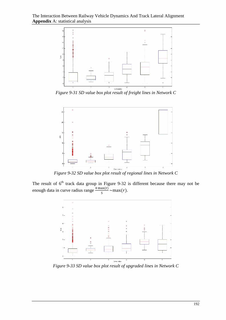
The Interaction Between Railway Vehicle Dynamics And Track Lateral Alignment
Appendix A: statistical analysis
192
Figure 9-31 SD value box plot result of freight lines in Network C
Figure 9-32 SD value box plot result of regional lines in Network C
The result of 6th
track data group in Figure 9-32 is different because there may not be
enough data in curve radius range
.
Figure 9-33 SD value box plot result of upgraded lines in Network C

The Interaction Between Railway Vehicle Dynamics And Track Lateral Alignment
Appendix A: statistical analysis
193
A.4 Fractal analysis results
From Figure 9-34 to Figure 9-43, the upper figure shows the fractal dimensions for each
1km long track along the whole DynoTrain recorded track data from Network A to C, and
the lower figures show the corresponded linear relationship between the vertical and lateral
track irregularity fractal dimensions. In all figures the blue lines represents vertical data
and black lines represents lateral data.
Figure 9-34 Vertical and lateral fractal dimension values in freight lines of Network A
Figure 9-35 Vertical and lateral fractal dimension values in regional lines of Network A

The Interaction Between Railway Vehicle Dynamics And Track Lateral Alignment
Appendix A: statistical analysis
194
Figure 9-36 Vertical and lateral fractal dimension values in upgraded lines of Network A
Figure 9-37 Vertical and lateral fractal dimension values in high speed lines of Network A

The Interaction Between Railway Vehicle Dynamics And Track Lateral Alignment
Appendix A: statistical analysis
195
Figure 9-38 Vertical and lateral fractal dimension values in regional lines of Network B
Figure 9-39 Vertical and lateral fractal dimension values in upgraded lines of Network B

The Interaction Between Railway Vehicle Dynamics And Track Lateral Alignment
Appendix A: statistical analysis
196
Figure 9-40 Vertical and lateral fractal dimension values in high speed lines of Network B
Figure 9-41 Vertical and lateral fractal dimension values in freight lines of Network C

The Interaction Between Railway Vehicle Dynamics And Track Lateral Alignment
Appendix A: statistical analysis
197
Figure 9-42 Vertical and lateral fractal dimension values in regional lines of Network C
Figure 9-43 Vertical and lateral fractal dimension values in upgraded lines of Network C

The Interaction Between Railway Vehicle Dynamics And Track Lateral Alignment
Appendix B: governing equations for boef track model
198
Appendix B GOVERNING EQUATIONS FOR
BOEF TRACK MODEL
From Figure 6-1, the movement at the point x can be analysed as the beam element model
is shown in Figure 9-44. The method of Euler-Bernoulli beam model is used here.
Figure 9-44 Beam Element Model
F(t)… input load that evaluated at the level the axle and summed for the passage of the
vehicles
M…beam bending moment
D…shear force
EI…the bending stiffness of the beam
k…vertical stiffness assuming a linear lateral response to load
c…vertical damping assuming a linear response to velocity
w(x,t)… beam deflection
x…the longitudinal distance from the load
f(x,t)…assumed distributed load on the beam
…mass density of the beam
A…cross section area of the beam.
From the diagram resolve vertically,

The Interaction Between Railway Vehicle Dynamics And Track Lateral Alignment
Appendix B: governing equations for boef track model
199
(
)
Equation 72
Equation 73
Take moment about the element,
(
)
Equation 74
Neglect terms, simplify:
Equation 75
From structures elastic theory it can be found:
Equation 76
Substituting the Equation 75 and Equation 76,
Equation 77
Therefore, substituting Equation 77 into Equation 73,
Equation 78
Rearrange,
Equation 79
Because there is no distributed load f, only a constant point load F for x>0 this equation
can be equated to 0. The governing PDE is
Equation 80
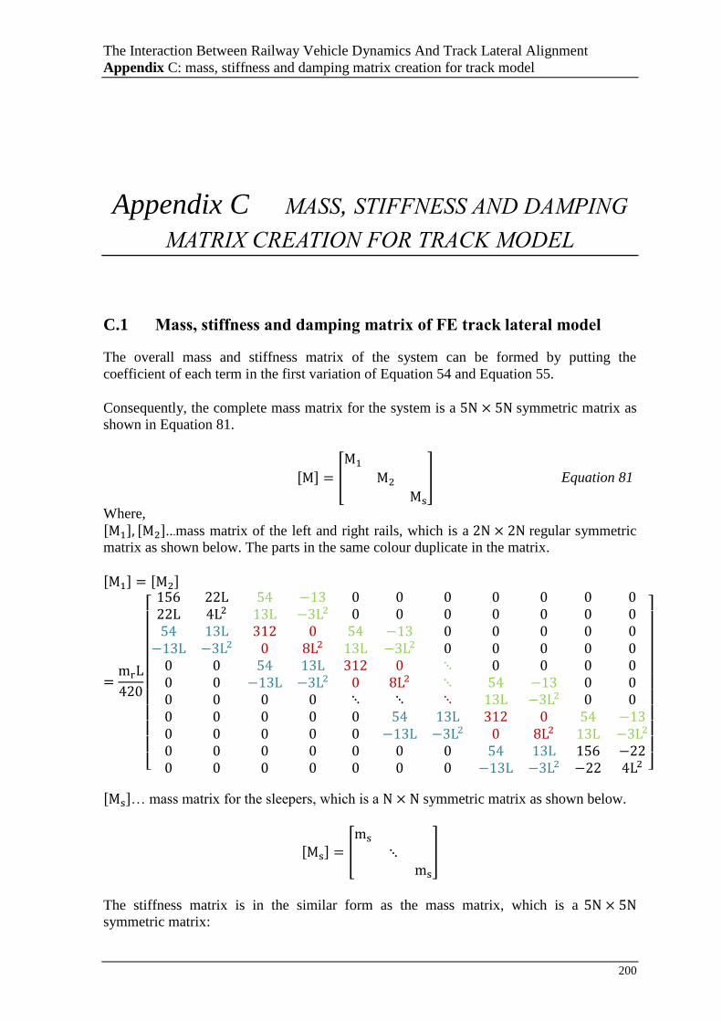
The Interaction Between Railway Vehicle Dynamics And Track Lateral Alignment
Appendix C: mass, stiffness and damping matrix creation for track model
200
Appendix C MASS, STIFFNESS AND DAMPING
MATRIX CREATION FOR TRACK MODEL
C.1 Mass, stiffness and damping matrix of FE track lateral model
The overall mass and stiffness matrix of the system can be formed by putting the
coefficient of each term in the first variation of Equation 54 and Equation 55.
Consequently, the complete mass matrix for the system is a symmetric matrix as
shown in Equation 81.
[
] Equation 81
Where,
...mass matrix of the left and right rails, which is a regular symmetric
matrix as shown below. The parts in the same colour duplicate in the matrix.
[
]
… mass matrix for the sleepers, which is a symmetric matrix as shown below.
[
]
The stiffness matrix is in the similar form as the mass matrix, which is a
symmetric matrix:

The Interaction Between Railway Vehicle Dynamics And Track Lateral Alignment
Appendix C: mass, stiffness and damping matrix creation for track model
201
[
] Equation 82
Where,
, … symmetric matrix:
[
]
, … symmetric matrix:
[
]
, … symmetric matrix:
[
]
… Symmetric matrix:
[
]
From the virtual work expression, the damping stiffness matrix can be found as a
symmetric matrix:
[
] Equation 83
Where,

The Interaction Between Railway Vehicle Dynamics And Track Lateral Alignment
Appendix C: mass, stiffness and damping matrix creation for track model
202
, … symmetric matrix:
[
]
, … symmetric matrix:
[
]
, … symmetric matrix:
[
]
… Symmetric matrix:
[
]

The Interaction Between Railway Vehicle Dynamics And Track Lateral Alignment
Appendix D: track model parameter selection
203
Appendix D TRACK MODEL PARAMETER
SELECTION
D.1 Traffic information on WCML
Table 9-2 shows the fleet composition information Actraff data found for the route on
WCML, which is split into three separate sections and taken for one period 13 x 4 week
periods in a year. The ‘name’ column actually contains the number of wheelsets for all
vehicles through that section, including other vehicles which are not listed in the table as
individually they each represent a small percentage of the traffic. In this case the traffic
levels are constant through all three sections, though they might not have been if there was
some S&C in the site and traffic had come onto or left the route.
Table 9-2 ACTRAFF data for the route

The Interaction Between Railway Vehicle Dynamics And Track Lateral Alignment
Appendix D: track model parameter selection
204
D.2 Lateral resistance parameters
Kish et al. [2] studied the track residual deflection in detail and summarised the track
lateral resistance parameters in Table 9-3. The lateral elastic breaking resistance Fe
depends on the peak lateral resistance Fp, and typically on the order of Fp/4.
Table 9-3 Track lateral resistance parameters Elastic
resistance
Fe (kN)
Elastic
displacement
we (mm)
Peak
resistance
Fp (kN)
Peak
displacement
wp (mm)
Weak, tamped track 2 – 2.5 0.6 – 0.7 8 – 9.8 3 – 3.5
Good quality track 3.3 – 4.5 1 – 1.3 13.3 – 17.8 4.8 – 6.4
Esveld [80] summarised the lateral resistance parameter from many test programmes and it
is shown in Table 9-4. These values are relatively lower than the values for typical track
system because the worst design case is considered.
Table 9-4 Lateral resistance characteristic values per sleeper Peak
resistance
Fp (kN)
Peak
displacement
wp (mm)
Min.
resistance
Fl (kN)
Displacement
wl(mm)
Loose Tamped/Relay (Weak) 5.2 15 5.2 40
Just Tamped (Medium) 7.1 10 6.2 40
Trafficked (Strong) 8.1 5 6.7 40
Le Pen [77] did a single sleeper push test and found the lateral resistance on unloaded track
for concrete sleepers are shown in the table below.
Table 9-5 Summary of lateral resistance test on unloaded track, concrete sleepers
Ballast category Lateral resistance/sleeper(kN)-peak within a deflection of 20mm
Minimum 20% less than 50% less than Maximum
Loose tamped/relay 4.2 5.2 5.9 6.9
Just tamped/undisturbed 5.9 7.1 8.3 11.8
Trafficked 5.4 8.1 10.3 15.7